On the Statistics of Smoking
Everyone knows smoking is bad for you. This post is about a narrower question: what does it look like when you try to show that from data, with the tools a statistics student is actually taught? I take three small, classic datasets that ship with R, fit the models that are appropriate to each, and spend most of the time on the inference rather than the fitting: the Wald test and its cousins, where the asymptotics quietly fail, what a Bayesian reading adds, and what a multivariate test buys you when you have several outcomes at once. 𐃏 The code is shown in full and the output is baked into the page. If you want to re-run it, every block is self-contained from the top of the page down, with the seed set.
Nothing here is new science. The point is the method: observational data, careful models, and conclusions stated at exactly the strength the evidence supports.
The question and the data
“Does smoking cause harm” is a causal question, and none of the data below comes from an experiment. Nobody randomised mothers to smoke. So every estimate on this page is an association, adjusted for whatever confounders happened to be recorded, and the gap between that and a causal effect is a matter of judgement, not computation. I will come back to this at the end, and once in the middle, where the Whickham data make the point by themselves.
Three datasets:
MASS::birthwt: 189 births at Baystate Medical Center, Springfield, Massachusetts, in 1986 (Hosmer and Lemeshow’s textbook data). The response is birth weight in grams (bwt) and its dichotomisation at 2500 g (low). The exposure is whether the mother smoked during pregnancy (smoke). Covariates: mother’s age, her weight at the last menstrual period (lwt, in pounds, which I convert to kilograms), race (coded white, black, other), history of hypertension (ht), uterine irritability (ui), number of previous premature labours (ptl) and physician visits in the first trimester (ftv).datasets::esoph: a case-control study of oesophageal cancer in Ille-et-Vilaine, France (Breslow and Day 1980). 88 cells cross-classify age group, alcohol consumption and tobacco consumption; each cell records how many of the people in it were cases (200 in total) and how many were controls (775). Because it is case-control, the sampling fixes the case and control totals, and only odds ratios are estimable.- The Whickham survey: 1314 women in Whickham, near Newcastle upon Tyne, classified as smokers or not in 1972-74 and followed up twenty years later for survival. I reconstruct the published 2 x 2 x 7 age-stratified table from Appleton, French and Vanderpump (1996), who used it to illustrate Simpson’s paradox. It is the same table the
mosaicDatapackage ships asWhickham; that package is not installed here, so the counts are typed in from the paper.
Set-up and a first look at the births
suppressPackageStartupMessages({
  library(MASS); library(car); library(lmtest); library(sandwich)
  library(mvtnorm); library(coda); library(arm)
})
set.seed(20261031)
options(width = 90)

bw <- birthwt
bw$smoke  <- factor(bw$smoke, labels = c("no", "yes"))
bw$race   <- factor(bw$race,  labels = c("white", "black", "other"))
bw$ht     <- factor(bw$ht);  bw$ui <- factor(bw$ui)
bw$lwt_kg <- bw$lwt * 0.4536                 # pounds -> kilograms

tab <- table(smoke = bw$smoke, low = bw$low)
print(tab)
print(round(prop.table(tab, 1), 3))          # row proportions: P(low | smoke)
print(round(t(sapply(split(bw$bwt, bw$smoke),
  function(x) c(n = length(x), mean = mean(x), sd = sd(x)))), 1))
     low
smoke  0  1
  no  86 29
  yes 44 30
     low
smoke     0     1
  no  0.748 0.252
  yes 0.595 0.405
      n   mean    sd
no  115 3055.7 752.7
yes  74 2771.9 659.6
Seventy-four of the 189 mothers smoked. Among them 41 percent of babies were low birth weight, against 25 percent among non-smokers, and the mean birth weight is about 280 g lower. That is the raw comparison; everything that follows asks how much of it survives adjustment and how sure we can be.
The oesophageal cancer cells
es <- esoph
es$tob <- as.integer(es$tobgp)               # tobacco dose as a 1..4 score
es$alc <- as.integer(es$alcgp)
cat("cells:", nrow(es), " cases:", sum(es$ncases), " controls:", sum(es$ncontrols), "\n")
agg <- aggregate(cbind(ncases, ncontrols) ~ tobgp, data = es, sum)
agg$prop_cases <- round(agg$ncases / (agg$ncases + agg$ncontrols), 3)
print(agg)
cells: 88  cases: 200  controls: 775
     tobgp ncases ncontrols prop_cases
1 0-9g/day     78       447      0.149
2    10-19     58       178      0.246
3    20-29     33        99      0.250
4      30+     31        51      0.378
The marginal fraction of cases climbs with tobacco dose, from 15 percent in the lightest group to 38 percent in the heaviest. But heavy smokers in this study also drink more and are older, so the marginal trend is not yet an answer.
Whickham, typed in from the paper
wh <- data.frame(
  age    = rep(c("18-24", "25-34", "35-44", "45-54", "55-64", "65-74", "75+"), each = 2),
  smoker = rep(c("yes", "no"), 7),
  alive  = c(53, 61, 121, 152, 95, 114, 103, 66, 64, 81, 7, 28, 0, 0),
  dead   = c( 2,  1,   3,   5, 14,   7,  27, 12, 51, 40, 29, 101, 13, 64))
wh$smoker <- factor(wh$smoker, levels = c("no", "yes"))
wh$age    <- factor(wh$age, levels = unique(wh$age))
wh$n      <- wh$alive + wh$dead
cat("total women:", sum(wh$n), "\n")
marg <- aggregate(cbind(alive, dead) ~ smoker, data = wh, sum)
marg$surv <- round(marg$alive / (marg$alive + marg$dead), 3)
print(marg)
total women: 1314
  smoker alive dead  surv
1     no   502  230 0.686
2    yes   443  139 0.761
Taken at face value, 76 percent of the smokers were alive at follow-up against 69 percent of the non-smokers. Smoking appears to be protective. Hold that thought.
Distributions
A regression model is a statement about the conditional distribution of the response, so the first job is to decide what family of distributions the responses plausibly come from, and to check.
Birth weight: approximately normal
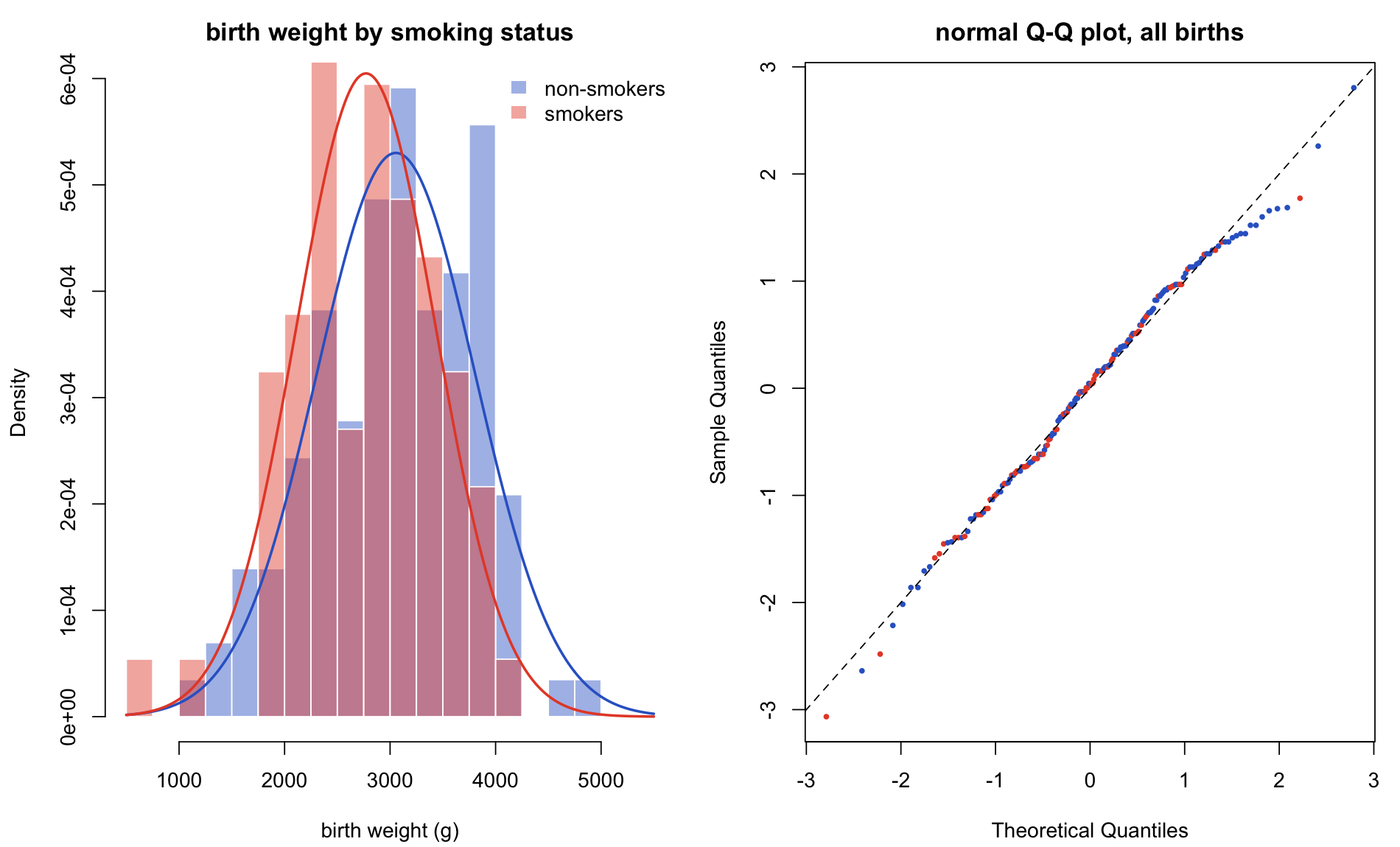
Birth weight is a continuous, positive quantity that is the sum of many small contributions, and in populations it is famously close to normal with a slightly heavy lower tail. Within each smoking group the histogram and the normal quantile plot bear that out; the Shapiro-Wilk test does not reject normality of the pooled weights, and the residual plots from the linear model later are unremarkable.
par(mfrow = c(1, 2), mar = c(4.2, 4.2, 2.5, 1))
brks <- seq(500, 5500, by = 250)
hist(bw$bwt[bw$smoke == "no"],  breaks = brks, freq = FALSE, col = rgb(0.2, 0.4, 0.8, 0.45),
     border = "white", xlab = "birth weight (g)", main = "birth weight by smoking status")
hist(bw$bwt[bw$smoke == "yes"], breaks = brks, freq = FALSE, col = rgb(0.9, 0.3, 0.2, 0.45),
     border = "white", add = TRUE)
xs <- seq(500, 5500, length.out = 300)
for (g in c("no", "yes")) {
  x <- bw$bwt[bw$smoke == g]
  lines(xs, dnorm(xs, mean(x), sd(x)), lwd = 2,
        col = if (g == "no") rgb(0.2, 0.4, 0.8) else rgb(0.9, 0.3, 0.2))
}
legend("topright", c("non-smokers", "smokers"), bty = "n",
       fill = c(rgb(0.2, 0.4, 0.8, 0.45), rgb(0.9, 0.3, 0.2, 0.45)), border = NA)
qqnorm(scale(bw$bwt), main = "normal Q-Q plot, all births", pch = 16, cex = 0.6,
       col = ifelse(bw$smoke == "yes", rgb(0.9, 0.3, 0.2), rgb(0.2, 0.4, 0.8)))
abline(0, 1, lty = 2)
print(shapiro.test(bw$bwt))
cat("skewness:", round(mean(scale(bw$bwt)^3), 3),
    "  excess kurtosis:", round(mean(scale(bw$bwt)^4) - 3, 3), "\n")
	Shapiro-Wilk normality test

data:  bw$bwt
W = 0.99244, p-value = 0.4353

skewness: -0.205   excess kurtosis: -0.144
The normal model for bwt is therefore defensible, and the linear model with a Gaussian error term is the natural choice. The slight negative skew (a longer tail of small babies) is real and is one reason the field also looks at the dichotomised outcome.
Low birth weight: Bernoulli, and in aggregate binomial
low is an indicator, so each birth is a Bernoulli trial with its own probability \(\pi_i\) that depends on the covariates. The counts in the 2 x 2 table above are then binomial: 30 of 74 smokers’ babies were low birth weight, and under a common probability \(\pi\) that is \(\mathrm{Binomial}(74, \pi)\). The variance of a Bernoulli is \(\pi(1-\pi)\), which is not constant in the mean, and the mean is confined to \((0, 1)\); both facts rule out ordinary least squares on the 0/1 outcome and motivate the logit link.
𐃏
# the two-sample comparison of proportions is a binomial problem
print(prop.test(c(30, 29), c(74, 115), correct = FALSE))
	2-sample test for equality of proportions without continuity correction

data:  c(30, 29) out of c(74, 115)
X-squared = 4.9237, df = 1, p-value = 0.02649
alternative hypothesis: two.sided
95 percent confidence interval:
 0.01607177 0.29039121
sample estimates:
   prop 1    prop 2
0.4054054 0.2521739
Oesophageal cancer: binomial per cell, and why not Poisson
Each of the 88 esoph cells holds a number of cases out of a known number of subjects, so the cell count of cases is binomial given the cell total. A Poisson model for the case count with an offset of \(\log(\text{cases} + \text{controls})\) is a common alternative for cohort data, where it estimates a rate ratio. In a case-control study the two do not agree unless cases are rare relative to controls, because the Poisson with an offset targets \(\log(\pi)\) while the binomial logit targets \(\log(\pi / (1 - \pi))\); here cases are 20 percent of the sample, far from rare. I fit both later and show the discrepancy. The following picture is the empirical check: observed cell proportions against those fitted by the binomial model with a linear tobacco score.
e_lin <- glm(cbind(ncases, ncontrols) ~ agegp + alcgp + tob, data = es, family = binomial)
par(mfrow = c(1, 2), mar = c(4.2, 4.4, 2.5, 1))
# (a) marginal proportion of cases by tobacco group with Wilson intervals
ci <- t(sapply(seq_len(nrow(agg)), function(i)
  prop.test(agg$ncases[i], agg$ncases[i] + agg$ncontrols[i], correct = FALSE)$conf.int))
plot(1:4, agg$prop_cases, ylim = c(0, 0.6), pch = 16, xaxt = "n", xlab = "tobacco (g/day)",
     ylab = "fraction of subjects who are cases", main = "marginal dose-response")
axis(1, 1:4, levels(es$tobgp)); arrows(1:4, ci[, 1], 1:4, ci[, 2], angle = 90, code = 3, length = 0.04)
# (b) observed vs fitted case counts per cell under the binomial model
plot(fitted(e_lin) * (es$ncases + es$ncontrols), es$ncases, pch = 16, cex = 0.7,
     xlab = "fitted cases per cell", ylab = "observed cases per cell",
     main = "binomial GLM, 88 cells"); abline(0, 1, lty = 2)
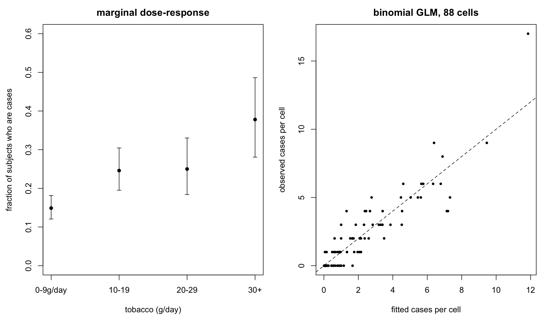
The marginal trend is steep and the fit is tight; the residual deviance is checked numerically in the regression section.
Regression
A linear model for birth weight
The exposure is smoke; the adjustment set is everything the data record that could plausibly affect birth weight and be associated with smoking: age, pre-pregnancy weight, race, hypertension, uterine irritability and prior premature labours. Coefficients are in grams.
m_lm <- lm(bwt ~ smoke + age + lwt_kg + race + ht + ui + ptl, data = bw)
print(summary(m_lm))
cat("\n95% CI for the smoking coefficient (grams):\n")
print(round(confint(m_lm)["smokeyes", ], 1))
Call:
lm(formula = bwt ~ smoke + age + lwt_kg + race + ht + ui + ptl,
    data = bw)

Residuals:
    Min      1Q  Median      3Q     Max
-1838.7  -454.5    57.6   465.1  1711.0

Coefficients:
            Estimate Std. Error t value Pr(>|t|)
(Intercept) 2934.132    311.450   9.421  < 2e-16 ***
smokeyes    -351.314    106.180  -3.309 0.001132 **
age           -4.093      9.440  -0.434 0.665091
lwt_kg         9.483      3.797   2.497 0.013416 *
raceblack   -488.196    149.604  -3.263 0.001318 **
raceother   -353.334    114.319  -3.091 0.002314 **
ht1         -586.836    200.841  -2.922 0.003925 **
ui1         -514.937    138.483  -3.718 0.000268 ***
ptl          -47.423    101.663  -0.466 0.641443
---
Signif. codes:  0 ‘***’ 0.001 ‘**’ 0.01 ‘*’ 0.05 ‘.’ 0.1 ‘ ’ 1

Residual standard error: 648.7 on 180 degrees of freedom
Multiple R-squared:  0.2424,	Adjusted R-squared:  0.2087
F-statistic: 7.197 on 8 and 180 DF,  p-value: 2.908e-08


95% CI for the smoking coefficient (grams):
 2.5 % 97.5 %
-560.8 -141.8
Holding the other covariates fixed, babies of smokers weigh an estimated 351 g less, with a 95 percent confidence interval of roughly 561 g to 142 g lighter. The adjustment moved the estimate away from zero relative to the raw 284 g difference. The reason is race: 52 of the 74 smokers are white, white mothers in this sample have the heaviest babies by some 300 g, and so the unadjusted comparison was partly comparing heavier white babies of smokers with lighter non-white babies of non-smokers, masking the within-race gap. The model explains a quarter of the variance (\(R^2 = 0.24\)); most of what makes one baby heavier than another is not in these columns.
A logistic model for low birth weight
Same covariates, response low, logit link. Exponentiated coefficients are odds ratios.
m_lo <- glm(low ~ smoke + age + lwt_kg + race + ht + ui + ptl, data = bw, family = binomial)
print(round(coef(summary(m_lo)), 4))
cat("\nodds ratios with Wald 95% intervals:\n")
print(round(exp(cbind(OR = coef(m_lo), confint.default(m_lo))), 3))
cat("\nodds ratios with profile-likelihood 95% intervals:\n")
print(round(exp(suppressMessages(confint(m_lo))), 3))
cat("\nnull deviance", round(m_lo$null.deviance, 2), "on", m_lo$df.null,
    "df;  residual deviance", round(deviance(m_lo), 2), "on", m_lo$df.residual, "df\n")
            Estimate Std. Error z value Pr(>|z|)
(Intercept)   0.4644     1.2047  0.3855   0.6999
smokeyes      0.9233     0.4009  2.3035   0.0213
age          -0.0271     0.0365 -0.7426   0.4577
lwt_kg       -0.0335     0.0153 -2.1915   0.0284
raceblack     1.2632     0.5265  2.3994   0.0164
raceother     0.8616     0.4392  1.9619   0.0498
ht1           1.8337     0.6918  2.6508   0.0080
ui1           0.7586     0.4594  1.6513   0.0987
ptl           0.5418     0.3463  1.5646   0.1177

odds ratios with Wald 95% intervals:
               OR 2.5 % 97.5 %
(Intercept) 1.591 0.150 16.870
smokeyes    2.518 1.148  5.523
age         0.973 0.906  1.045
lwt_kg      0.967 0.939  0.996
raceblack   3.537 1.260  9.925
raceother   2.367 1.001  5.598
ht1         6.257 1.613 24.277
ui1         2.135 0.868  5.254
ptl         1.719 0.872  3.389

odds ratios with profile-likelihood 95% intervals:
            2.5 % 97.5 %
(Intercept) 0.154 17.737
smokeyes    1.161  5.645
age         0.905  1.044
lwt_kg      0.937  0.995
raceblack   1.264 10.126
raceother   1.013  5.725
ht1         1.669 26.520
ui1         0.859  5.271
ptl         0.881  3.478

null deviance 234.67 on 188 df;  residual deviance 201.43 on 180 df
The adjusted odds of a low-birth-weight baby are about 2.5 times higher for smokers (Wald 95 percent interval 1.15 to 5.52). The profile-likelihood interval, 1.16 to 5.65, is slightly wider and shifted right; the two agree well here because the coefficient is moderate and the sample is not tiny. Look at ht (hypertension), estimated from only 12 mothers: Wald gives 1.6 to 24.3, profile gives 1.7 to 26.5. The gap is the first hint of the Wald test’s weakness with sparse cells, which I take up below.
Dose-response in the oesophageal data
Tobacco consumption is recorded as four ordered groups. A factor with four levels spends three parameters; a linear score in the ordered groups spends one and asserts that each step up in dose multiplies the odds by the same amount. The likelihood-ratio test between the two tells me whether the single-slope model is losing anything.
e_fac <- glm(cbind(ncases, ncontrols) ~ agegp + alcgp + tobgp, data = es, family = binomial)
e_lin <- glm(cbind(ncases, ncontrols) ~ agegp + alcgp + tob,   data = es, family = binomial)
print(anova(e_lin, e_fac, test = "Chisq"))
cat("\nodds ratio per tobacco category step (adjusted for age and alcohol):\n")
print(round(exp(c(OR = coef(e_lin)["tob"], confint.default(e_lin)["tob", ])), 3))
cat("\ngoodness of fit: residual deviance", round(deviance(e_lin), 2), "on", df.residual(e_lin),
    "df; Pearson X2", round(sum(residuals(e_lin, "pearson")^2), 2), "\n")

# Poisson with offset: targets the log rate, not the log odds
e_poi <- glm(ncases ~ agegp + alcgp + tob + offset(log(ncases + ncontrols)), data = es, family = poisson)
cat("\ntobacco slope, binomial-logit vs Poisson-log:\n")
print(round(c(binomial = coef(e_lin)["tob"], poisson = coef(e_poi)["tob"]), 4))
Analysis of Deviance Table

Model 1: cbind(ncases, ncontrols) ~ agegp + alcgp + tob
Model 2: cbind(ncases, ncontrols) ~ agegp + alcgp + tobgp
  Resid. Df Resid. Dev Df Deviance Pr(>Chi)
1        78     85.866
2        76     82.337  2   3.5293   0.1712

odds ratio per tobacco category step (adjusted for age and alcohol):
OR.tob  2.5 % 97.5 %
 1.541  1.275  1.862

goodness of fit: residual deviance 85.87 on 78 df; Pearson X2 88.78

tobacco slope, binomial-logit vs Poisson-log:
binomial.tob  poisson.tob
      0.4322       0.2336
Dropping the two extra parameters costs 3.5 units of deviance on 2 degrees of freedom (\(p = 0.17\)), so the linear-in-dose model is adequate. Each step up in the tobacco scale multiplies the odds of being a case by about 1.54 (1.27 to 1.86), adjusting for age and alcohol. The residual deviance of 86 on 78 degrees of freedom is consistent with a binomial fit; the data are not overdispersed.
The Poisson slope of 0.23 is about half the logit slope of 0.43. That is not a mistake in either model; it is the difference between a rate ratio and an odds ratio when the outcome is common. In a case-control design the odds ratio is the estimand the sampling permits, so the binomial fit is the one to report.
The confounder you cannot ignore: Whickham
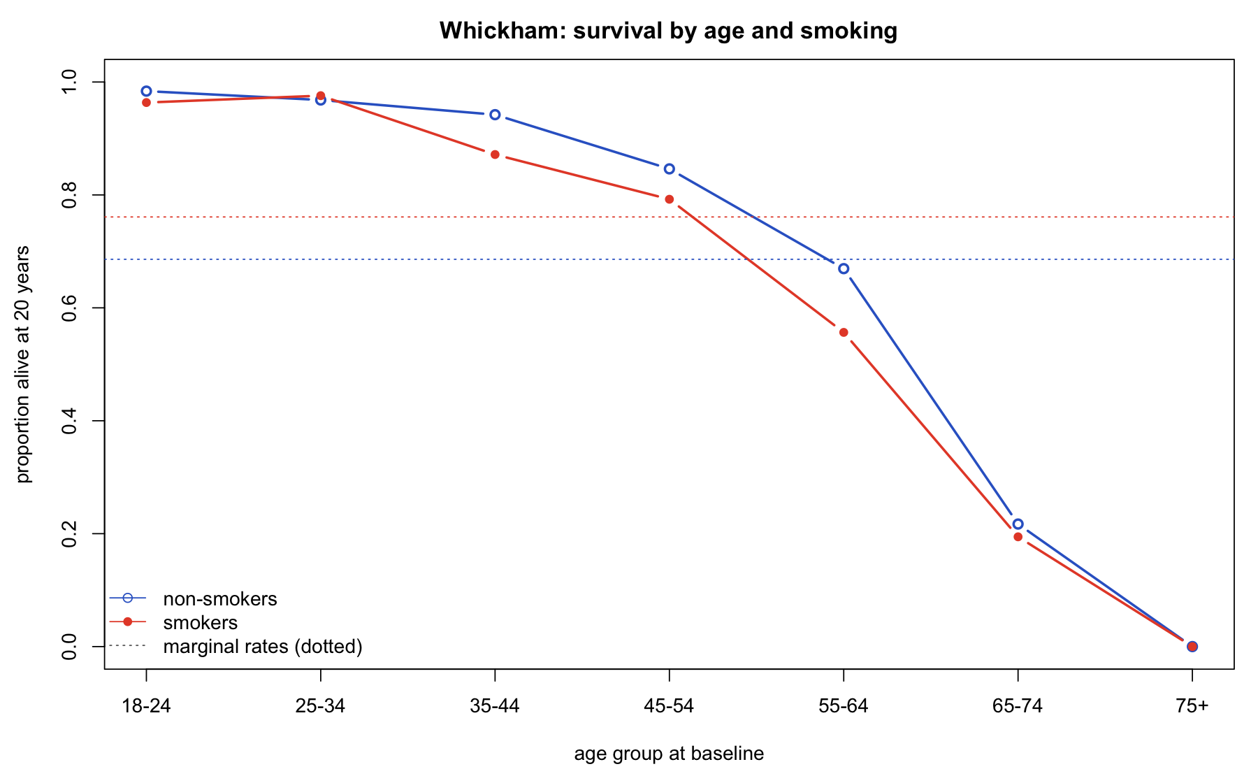
Back to the women of Whickham, where smokers appeared to survive better. Stratify by age.
wh$surv <- wh$alive / wh$n
sv <- xtabs(surv ~ age + smoker, data = wh)
par(mar = c(4.2, 4.4, 2.5, 1))
matplot(1:7, sv, type = "b", pch = c(1, 16), lty = 1, lwd = 2, col = c(rgb(0.2, 0.4, 0.8), rgb(0.9, 0.3, 0.2)),
        xaxt = "n", xlab = "age group at baseline", ylab = "proportion alive at 20 years",
        main = "Whickham: survival by age and smoking", ylim = c(0, 1))
axis(1, 1:7, levels(wh$age))
abline(h = marg$surv, lty = 3, col = c(rgb(0.2, 0.4, 0.8), rgb(0.9, 0.3, 0.2)))
legend("bottomleft", c("non-smokers", "smokers", "marginal rates (dotted)"),
       col = c(rgb(0.2, 0.4, 0.8), rgb(0.9, 0.3, 0.2), "grey40"), pch = c(1, 16, NA), lty = c(1, 1, 3), bty = "n")
arr <- array(0, dim = c(2, 2, 7),
             dimnames = list(smoker = c("yes", "no"), status = c("alive", "dead"), age = levels(wh$age)))
for (i in seq_len(nrow(wh)))
  arr[as.character(wh$smoker[i]), , as.character(wh$age[i])] <- c(wh$alive[i], wh$dead[i])
print(mantelhaen.test(arr))

w_marg <- glm(cbind(alive, dead) ~ smoker,       data = wh, family = binomial)
w_adj  <- glm(cbind(alive, dead) ~ smoker + age, data = wh, family = binomial)
cat("odds ratio of survival for smokers, marginal:     ",
    round(exp(coef(w_marg)["smokeryes"]), 3), "\n")
cat("odds ratio of survival for smokers, age-adjusted: ",
    round(exp(coef(w_adj)["smokeryes"]), 3), " 95% CI",
    round(exp(confint.default(w_adj)["smokeryes", ]), 3), "\n")
	Mantel-Haenszel chi-squared test with continuity correction

data:  arr
Mantel-Haenszel X-squared = 5.435, df = 1, p-value = 0.01974
alternative hypothesis: true common odds ratio is not equal to 1
95 percent confidence interval:
 0.4632784 0.9247150
sample estimates:
common odds ratio
        0.6545231

odds ratio of survival for smokers, marginal:      1.46
odds ratio of survival for smokers, age-adjusted:  0.652  95% CI 0.461 0.923
In every age band from 35 to 74, smokers die more; in the two youngest bands the rates are within a point or two of each other, and nobody in the 75+ group of either kind survived twenty years. Marginally, smokers die less. The reconciliation is in the age structure: in 1972 the smokers were concentrated in the young and middle-aged groups, where almost everyone survives, and the non-smokers included most of the elderly. The age-adjusted odds ratio for survival is 0.65 (0.46 to 0.92), and the Mantel-Haenszel common odds ratio agrees. This is Simpson’s paradox in its cleanest form and it is why “adjusting for covariates” is not a nicety in observational work; the sign of the answer depends on it.
Hypothesis tests, with Wald at the centre
The Wald statistic
Let \(\hat\theta\) be the maximum-likelihood estimate of a parameter vector and \(\hat V\) a consistent estimate of its asymptotic covariance, usually the inverse of the observed or expected Fisher information evaluated at \(\hat\theta\). For a single coefficient and the hypothesis \(H_0: \theta_j = \theta_{j0}\), the Wald statistic is
\begin{equation} W = \frac{(\hat\theta_j - \theta_{j0})^2}{\hat V_{jj}} = z^2, \qquad z = \frac{\hat\theta_j - \theta_{j0}}{\mathrm{se}(\hat\theta_j)}, \end{equation}
and under \(H_0\), as the sample grows, \(z \to N(0,1)\) and \(W \to \chi^2_1\). For \(q\) simultaneous linear restrictions \(H_0: R\theta = r\), with \(R\) a \(q \times p\) matrix of full row rank,
\begin{equation} W = (R\hat\theta - r)^\top \left(R \hat V R^\top\right)^{-1} (R\hat\theta - r) \;\xrightarrow{d}\; \chi^2_q . \end{equation}
Every z value and Pr(>|z|) in a glm summary is a Wald test; every t value in an lm summary is the same thing with the normal replaced by a \(t\) distribution because the error variance is estimated. The attraction is that one fit yields every Wald test you like; the cost is that it trusts the quadratic approximation of the log-likelihood at the maximum, and only at the maximum.
By hand, then with car and lmtest
For the logistic model, the single-coefficient Wald test for smoking and the joint test that both race contrasts are zero:
b <- coef(m_lo); V <- vcov(m_lo)
W_smoke <- b["smokeyes"]^2 / V["smokeyes", "smokeyes"]
cat("Wald for smoke:  W =", round(W_smoke, 4), "  p =", signif(pchisq(W_smoke, 1, lower.tail = FALSE), 4),
    "  (z^2 from the summary:", round(coef(summary(m_lo))["smokeyes", "z value"]^2, 4), ")\n")

R <- matrix(0, nrow = 2, ncol = length(b), dimnames = list(NULL, names(b)))
R[1, "raceblack"] <- 1; R[2, "raceother"] <- 1
Rb <- R %*% b
W_race <- drop(t(Rb) %*% solve(R %*% V %*% t(R)) %*% Rb)
cat("Wald for race (q = 2):  W =", round(W_race, 4), "  p =", signif(pchisq(W_race, 2, lower.tail = FALSE), 4), "\n\n")

print(linearHypothesis(m_lo, c("raceblack = 0", "raceother = 0"), test = "Chisq"))
print(waldtest(update(m_lo, . ~ . - race), m_lo, test = "Chisq"))
Wald for smoke:  W = 5.3059   p = 0.02125   (z^2 from the summary: 5.3059 )
Wald for race (q = 2):  W = 7.0059   p = 0.03011


Linear hypothesis test:
raceblack = 0
raceother = 0

Model 1: restricted model
Model 2: low ~ smoke + age + lwt_kg + race + ht + ui + ptl

  Res.Df Df  Chisq Pr(>Chisq)
1    182
2    180  2 7.0059    0.03011 *
---
Signif. codes:  0 ‘***’ 0.001 ‘**’ 0.01 ‘*’ 0.05 ‘.’ 0.1 ‘ ’ 1
Wald test

Model 1: low ~ smoke + age + lwt_kg + ht + ui + ptl
Model 2: low ~ smoke + age + lwt_kg + race + ht + ui + ptl
  Res.Df Df  Chisq Pr(>Chisq)
1    182
2    180  2 7.0059    0.03011 *
---
Signif. codes:  0 ‘***’ 0.001 ‘**’ 0.01 ‘*’ 0.05 ‘.’ 0.1 ‘ ’ 1
The hand computation and the packaged ones agree to every printed digit, as they must; they are the same formula. For the linear model the same joint hypothesis gives an \(F\) statistic, which is the Wald statistic divided by \(q\) with the \(\chi^2\) reference replaced by \(F_{q,\,n-p}\):
print(linearHypothesis(m_lm, c("raceblack = 0", "raceother = 0")))
Linear hypothesis test:
raceblack = 0
raceother = 0

Model 1: restricted model
Model 2: bwt ~ smoke + age + lwt_kg + race + ht + ui + ptl

  Res.Df      RSS Df Sum of Sq      F    Pr(>F)
1    182 82293521
2    180 75741025  2   6552496 7.7861 0.0005713 ***
---
Signif. codes:  0 ‘***’ 0.001 ‘**’ 0.01 ‘*’ 0.05 ‘.’ 0.1 ‘ ’ 1
Wald, likelihood ratio and score on the same hypothesis
Three asymptotically equivalent tests of \(H_0: \beta_{\text{smoke}} = 0\) in the logistic model. The likelihood-ratio statistic is twice the drop in log-likelihood when the constraint is imposed; the score (Rao) statistic measures the gradient of the log-likelihood at the constrained estimate, scaled by the information there. Wald looks at the unconstrained maximum, LR at both, score at the constrained one.
m_lo0 <- update(m_lo, . ~ . - smoke)
LR    <- 2 * (as.numeric(logLik(m_lo)) - as.numeric(logLik(m_lo0)))
cat("Wald  W =", round(W_smoke, 3), "\n")
cat("LR    G =", round(LR, 3), "   (deviance difference", round(deviance(m_lo0) - deviance(m_lo), 3), ")\n")
rao <- anova(m_lo0, m_lo, test = "Rao")
cat("Score S =", round(rao$Rao[2], 3), "\n")
cat("p-values (chi-square, 1 df):", signif(pchisq(c(W_smoke, LR, rao$Rao[2]), 1, lower.tail = FALSE), 3), "\n")
Wald  W = 5.306
LR    G = 5.489    (deviance difference 5.489 )
Score S = 5.477
p-values (chi-square, 1 df): 0.0213 0.0191 0.0193
All three land between 5.3 and 5.5 with \(p\) around 0.02. The picture below is why they agree here and why they would not always: the profile log-likelihood for \(\beta_{\text{smoke}}\) is nearly quadratic over the region that matters, and the Wald test is precisely the test you get by pretending it is exactly quadratic. 𐃏
sm   <- as.integer(bw$smoke == "yes")
grid <- seq(-0.6, 2.6, by = 0.05)
prof <- sapply(grid, function(b0) as.numeric(logLik(
  glm(low ~ age + lwt_kg + race + ht + ui + ptl + offset(b0 * sm), data = bw, family = binomial))))
l_hat <- as.numeric(logLik(m_lo)); b_hat <- b["smokeyes"]; se_hat <- sqrt(V["smokeyes", "smokeyes"])
quad  <- l_hat - 0.5 * ((grid - b_hat) / se_hat)^2
par(mar = c(4.2, 4.4, 2.5, 1))
plot(grid, prof, type = "l", lwd = 2, xlab = expression(beta[smoke]), ylab = "log-likelihood",
     main = "profile log-likelihood vs the Wald quadratic")
lines(grid, quad, lty = 2, lwd = 2, col = rgb(0.9, 0.3, 0.2))
abline(h = l_hat - qchisq(0.95, 1) / 2, lty = 3); abline(v = 0, col = "grey60")
legend("bottomright", c("profile likelihood", "quadratic (Wald) approximation", "95% likelihood cut-off"),
       lty = c(1, 2, 3), lwd = c(2, 2, 1), col = c("black", rgb(0.9, 0.3, 0.2), "black"), bty = "n")
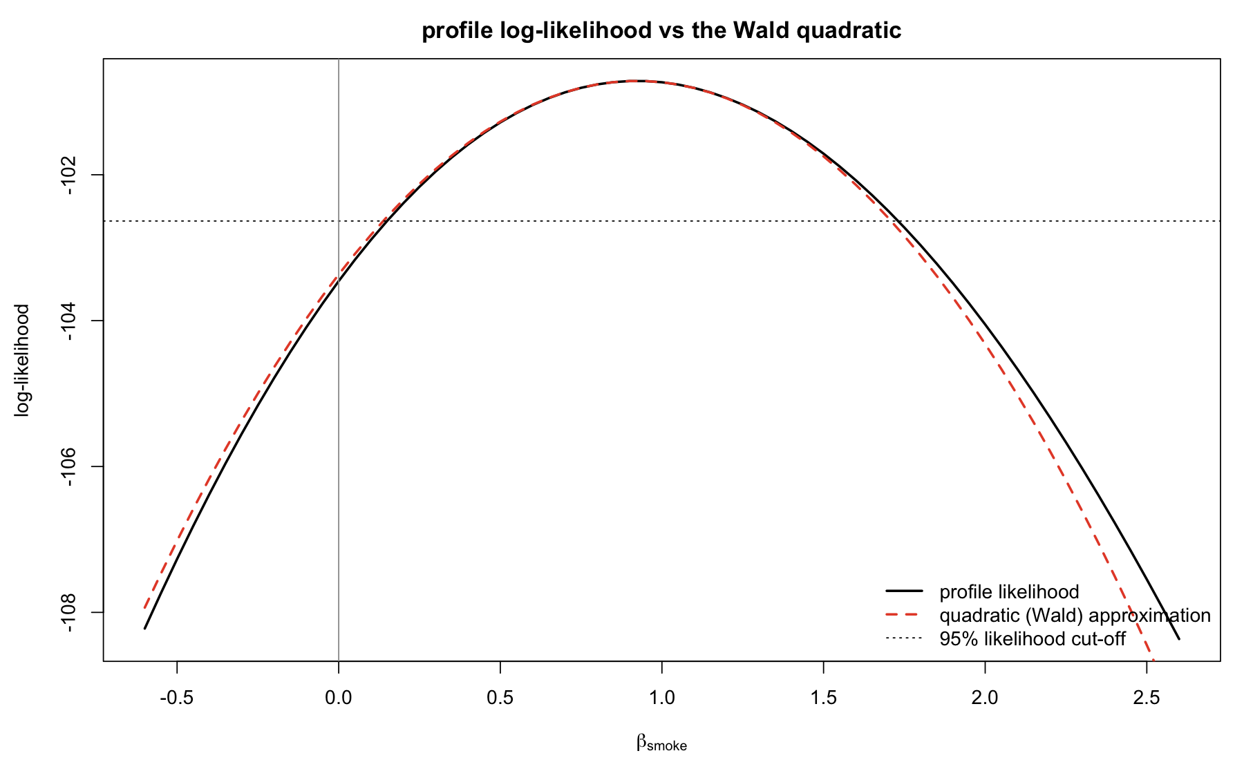
Where the dotted horizontal line cuts the solid curve is the profile-likelihood confidence interval; where it cuts the dashed parabola is the Wald interval. The parabola is slightly too narrow on the right and too wide on the left, which is the asymmetry seen in the odds-ratio table.
When Wald misbehaves
The Hauck-Donner effect. In logistic regression the Wald statistic is not monotone in the evidence. As the data move towards complete separation, the estimated coefficient grows without bound but its standard error grows faster, so \(z\) shrinks towards zero exactly when the evidence against \(H_0\) is strongest (Hauck and Donner 1977). The likelihood-ratio statistic keeps increasing. A small constructed example: 40 points, the outcome is 1 when \(x > 0\) except for one contrary point on each side at rank \(k\) from the boundary, so smaller \(k\) means less overlap.
set.seed(1)
n <- 40; x <- sort(rnorm(n))
neg <- rev(which(x < 0)); pos <- which(x > 0)       # both ordered by distance from zero
hd <- function(k) {
  y <- as.integer(x > 0)
  if (k > 0) { fl <- c(neg[k], pos[k]); y[fl] <- 1 - y[fl] }
  f  <- suppressWarnings(glm(y ~ x, family = binomial)); f0 <- glm(y ~ 1, family = binomial)
  cs <- coef(summary(f))["x", ]
  c(k = k, beta = unname(cs["Estimate"]), se = unname(cs["Std. Error"]),
    wald = unname(cs["z value"]^2), lrt = f0$deviance - f$deviance)
}
hd_tab <- t(sapply(c(10, 8, 6, 5, 4, 3, 2, 1, 0), hd))
par(mar = c(4.2, 4.4, 2.5, 1))
plot(hd_tab[, "lrt"], hd_tab[, "wald"], type = "b", pch = 16, lwd = 2,
     xlab = "likelihood-ratio statistic (evidence against the null)", ylab = "Wald statistic",
     main = "Hauck-Donner: Wald falls as the evidence grows")
text(hd_tab[, "lrt"], hd_tab[, "wald"], labels = paste0("k=", hd_tab[, "k"]),
     pos = ifelse(hd_tab[, "k"] == 4, 1, 3), cex = 0.75)
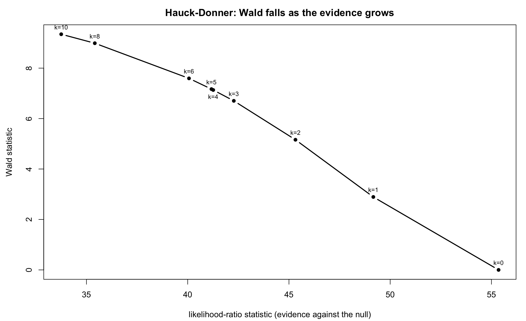
print(round(hd_tab, 3))
      k    beta         se  wald    lrt
[1,] 10   5.163      1.689 9.345 33.754
[2,]  8   5.651      1.885 8.989 35.413
[3,]  6   7.473      2.712 7.595 40.064
[4,]  5   8.057      3.009 7.168 41.174
[5,]  4   8.106      3.035 7.134 41.261
[6,]  3   8.724      3.369 6.703 42.277
[7,]  2  11.275      4.963 5.161 45.321
[8,]  1  18.482     10.868 2.892 49.167
[9,]  0 420.471 131640.076 0.000 55.352
At \(k = 0\) the data are perfectly separated: the MLE does not exist, R’s estimate is whatever the iteration stopped at, the standard error is astronomical and the Wald test reports no evidence at all against a null hypothesis that the data reject as decisively as 40 points can. The LR statistic of 55 tells the truth. In practice the warning signs are a huge coefficient with a huger standard error and a glm warning that fitted probabilities of 0 or 1 occurred.
Small samples and sparse cells. The \(\chi^2\) reference is asymptotic. With 12 hypertensive mothers, the Wald interval for ht above is visibly off the profile interval, and in smaller tables than this it can be badly anticonservative or badly conservative depending on the direction of the skew. Profile-likelihood intervals (confint on a glm) and LR tests are the better default whenever a cell is thin.
Parameterisation. The Wald test is not invariant to reparameterisation: testing \(\beta = 0\) and testing \(e^{\beta} = 1\) give different Wald statistics because the standard error is transported by the delta method and the quadratic approximation is taken on a different scale. The LR and score tests are invariant. This is the formal version of the asymmetry in the odds-ratio intervals: the Wald interval is symmetric on the log-odds scale and lopsided after exponentiating.
Robust (sandwich) standard errors
The model-based covariance \(\hat V = \mathcal{I}(\hat\theta)^{-1}\) is correct only if the variance model is. The sandwich estimator \(\hat V_{\text{HC}} = \hat B^{-1} \hat M \hat B^{-1}\), with \(\hat B\) the Hessian (bread) and \(\hat M\) the outer product of the score contributions (meat), is consistent for the covariance of \(\hat\theta\) under heteroskedasticity or other misspecification of the second moment, though not of the mean. Plugging it into the Wald statistic gives a robust Wald test.
cat("linear model, smoking coefficient:\n")
print(round(rbind(model_based = coeftest(m_lm)["smokeyes", ],
                  HC3         = coeftest(m_lm, vcov = vcovHC(m_lm, type = "HC3"))["smokeyes", ]), 4))
print(bptest(m_lm))
cat("logistic model, smoking coefficient:\n")
print(round(rbind(model_based = coeftest(m_lo)["smokeyes", ],
                  sandwich    = coeftest(m_lo, vcov = sandwich(m_lo))["smokeyes", ]), 4))
linear model, smoking coefficient:
             Estimate Std. Error t value Pr(>|t|)
model_based -351.3142   106.1801 -3.3087   0.0011
HC3         -351.3142   109.6914 -3.2028   0.0016

	studentized Breusch-Pagan test

data:  m_lm
BP = 11.499, df = 8, p-value = 0.175

logistic model, smoking coefficient:
            Estimate Std. Error z value Pr(>|z|)
model_based   0.9233     0.4009  2.3035   0.0213
sandwich      0.9233     0.3857  2.3937   0.0167
For birth weight the robust standard error is within a few grams of the model-based one and the Breusch-Pagan test finds no heteroskedasticity worth the name. For the logistic model the sandwich standard error is a little smaller, which is what you tend to see when the binomial variance is, if anything, slightly over-stated by the model. Neither changes the conclusion, which is the point of checking: a robust standard error that moved things a lot would be a sign that the mean model, not just the variance, was wrong.
Bayesian readings
A Beta-binomial analysis of the smoking proportion
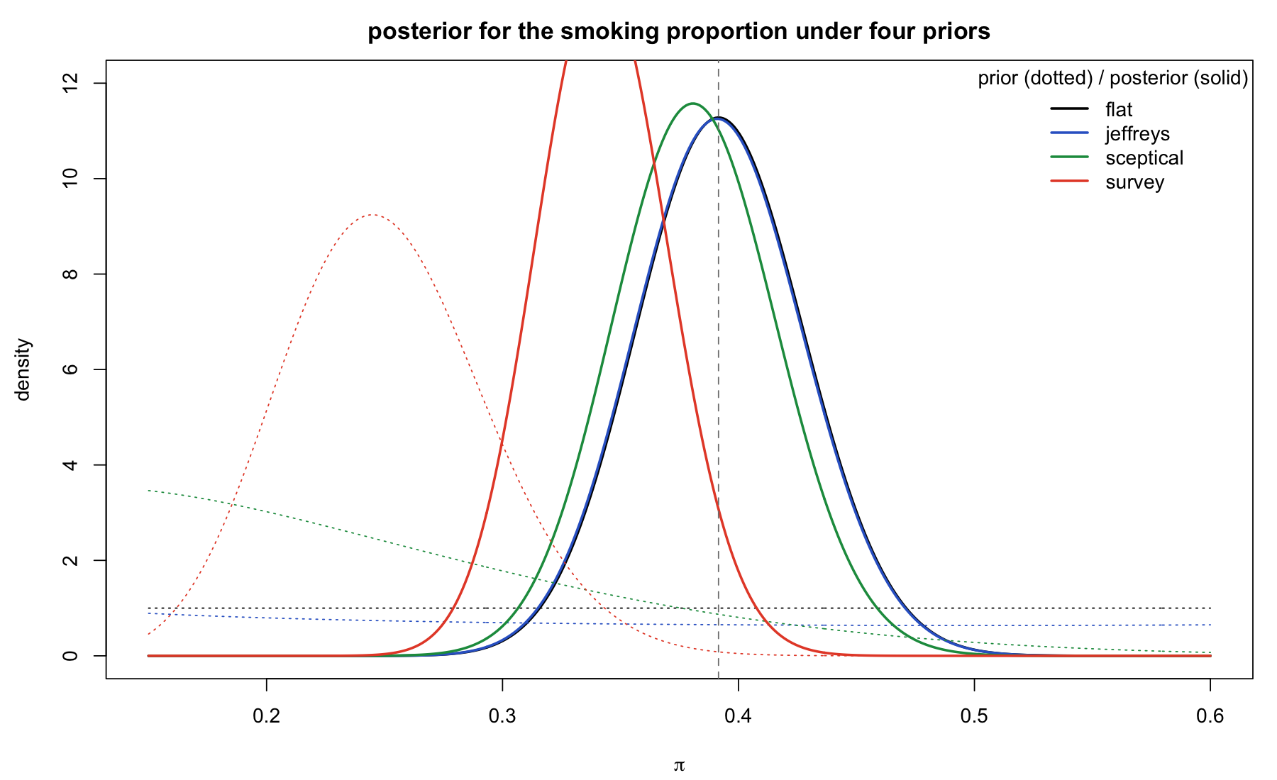
What fraction of mothers in this population smoke? The likelihood is \(\mathrm{Binomial}(189, \pi)\) with 74 successes, and with a \(\mathrm{Beta}(a, b)\) prior the posterior is \(\mathrm{Beta}(a + 74,\; b + 115)\) in closed form. I try four priors: flat, Jeffreys, a sceptical prior centred at 20 percent, and a fairly confident prior centred at 25 percent that stands in for an external survey estimate of smoking prevalence in pregnancy at the time. 𐃏
s <- sum(bw$smoke == "yes"); n_bw <- nrow(bw)
priors <- rbind(flat = c(1, 1), jeffreys = c(0.5, 0.5), sceptical = c(2, 8), survey = c(25, 75))
cols <- c("black", rgb(0.2, 0.4, 0.8), rgb(0.1, 0.6, 0.3), rgb(0.9, 0.3, 0.2))
xs <- seq(0.15, 0.6, length.out = 400)
par(mar = c(4.2, 4.4, 2.5, 1))
plot(NA, xlim = range(xs), ylim = c(0, 12), xlab = expression(pi), ylab = "density",
     main = "posterior for the smoking proportion under four priors")
for (i in seq_len(nrow(priors))) {
  a <- priors[i, 1] + s; bb <- priors[i, 2] + n_bw - s
  lines(xs, dbeta(xs, a, bb), lwd = 2, col = cols[i])
  lines(xs, dbeta(xs, priors[i, 1], priors[i, 2]), lty = 3, col = cols[i])
}
abline(v = s / n_bw, lty = 2, col = "grey50")
legend("topright", rownames(priors), col = cols, lwd = 2, bty = "n", title = "prior (dotted) / posterior (solid)")
post <- t(apply(priors, 1, function(ab) {
  a <- ab[1] + s; bb <- ab[2] + n_bw - s
  c(prior_mean = ab[1] / sum(ab), post_mean = a / (a + bb),
    lo95 = qbeta(0.025, a, bb), hi95 = qbeta(0.975, a, bb), P_pi_gt_0.3 = 1 - pbeta(0.3, a, bb))
}))
print(round(post, 4))
p_hat <- s / n_bw
cat("\nfrequentist, for comparison:\n")
cat("  Wald   95% CI:", round(p_hat + c(-1, 1) * qnorm(0.975) * sqrt(p_hat * (1 - p_hat) / n_bw), 4), "\n")
cat("  Wilson 95% CI:", round(prop.test(s, n_bw, correct = FALSE)$conf.int, 4), "\n")
          prior_mean post_mean   lo95   hi95 P_pi_gt_0.3
flat            0.50    0.3927 0.3247 0.4627      0.9967
jeffreys        0.50    0.3921 0.3240 0.4623      0.9964
sceptical       0.20    0.3819 0.3158 0.4503      0.9929
survey          0.25    0.3426 0.2890 0.3982      0.9388

frequentist, for comparison:
  Wald   95% CI: 0.3219 0.4611
  Wilson 95% CI: 0.3248 0.4626
With 189 observations the flat and Jeffreys posteriors are indistinguishable from each other and from the Wilson interval; the sceptical prior, worth ten observations, shifts the mean by a point. Only the survey prior, worth a hundred pseudo-observations, moves the interval materially, and even then the posterior probability that more than 30 percent of this population smokes stays above 0.9. The data dominate; the prior sensitivity analysis is how you demonstrate that rather than assert it.
Bayesian logistic regression by Laplace approximation and Metropolis sampling
The same logistic model, now with independent normal priors on the coefficients: \(N(0, 10^2)\) on the intercept and \(N(0, 2.5^2)\) on each slope, with the continuous covariates standardised so that a prior scale of 2.5 means the same thing for every column. This is the weakly informative default of Gelman and colleagues: it rules out absurd effects (an odds ratio of a million) and nothing else. The log-posterior is
\begin{equation} \log p(\beta \mid y) = \sum_{i=1}^{n} \left[ y_i\, \mathbf{x}_i^\top\beta - \log\!\left(1 + e^{\mathbf{x}_i^\top\beta}\right) \right] - \sum_{j} \frac{\beta_j^2}{2\tau_j^2} + \text{const}, \end{equation}
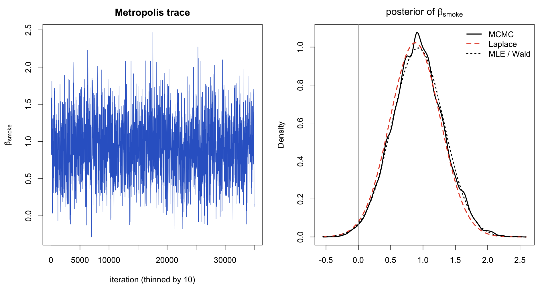
which has no closed form. Two routes. The Laplace approximation finds the mode \(\tilde\beta\) and uses the negative inverse Hessian there as a covariance, so the posterior is approximated by \(N(\tilde\beta, \tilde\Sigma)\); for a logistic likelihood with a flat prior this would reproduce the MLE and its Wald covariance exactly, which is the Bayesian reading of why Wald works when it works. Random-walk Metropolis then samples the exact posterior, using the Laplace covariance to tune the proposal.
X  <- model.matrix(low ~ smoke + age + lwt_kg + race + ht + ui + ptl, data = bw)
y  <- bw$low
Xs <- X
for (v in c("age", "lwt_kg", "ptl")) Xs[, v] <- (X[, v] - mean(X[, v])) / sd(X[, v])
prior_sd <- c(10, rep(2.5, ncol(Xs) - 1))

log_post <- function(beta) {
  eta <- drop(Xs %*% beta)
  sum(y * eta - log1p(exp(eta))) + sum(dnorm(beta, 0, prior_sd, log = TRUE))
}
# Laplace: mode and curvature
opt   <- optim(rep(0, ncol(Xs)), log_post, method = "BFGS", hessian = TRUE,
               control = list(fnscale = -1, maxit = 5000))
mode_ <- opt$par; Sigma <- solve(-opt$hessian)
names(mode_) <- colnames(Xs); dimnames(Sigma) <- list(colnames(Xs), colnames(Xs))

# Metropolis with a multivariate-normal proposal scaled by the usual 2.38^2 / d
set.seed(20261031)
n_iter <- 40000; d <- ncol(Xs)
draws  <- matrix(NA_real_, n_iter, d, dimnames = list(NULL, colnames(Xs)))
cur <- mode_; lp_cur <- log_post(cur); acc <- 0
prop_S <- (2.38^2 / d) * Sigma
for (i in seq_len(n_iter)) {
  cand <- drop(rmvnorm(1, cur, prop_S)); lp_cand <- log_post(cand)
  if (log(runif(1)) < lp_cand - lp_cur) { cur <- cand; lp_cur <- lp_cand; acc <- acc + 1 }
  draws[i, ] <- cur
}
draws <- draws[-(1:5000), ]                      # burn-in
cat("acceptance rate:", round(acc / n_iter, 3), "\n")
cat("effective sample sizes (first four):", round(effectiveSize(mcmc(draws))[1:4]), "\n\n")

mle_s <- glm(y ~ Xs - 1, family = binomial)    # MLE on the same standardised design
cmp <- cbind(MLE = coef(mle_s), Wald_se = sqrt(diag(vcov(mle_s))),
             Laplace = mode_, Laplace_sd = sqrt(diag(Sigma)),
             MCMC_mean = colMeans(draws), MCMC_sd = apply(draws, 2, sd))
rownames(cmp) <- colnames(Xs)
print(round(cmp, 3))
acceptance rate: 0.275
effective sample sizes (first four): 1271 1231 1192 1244

               MLE Wald_se Laplace Laplace_sd MCMC_mean MCMC_sd
(Intercept) -2.030   0.402  -1.955      0.387    -2.029   0.387
smokeyes     0.923   0.401   0.880      0.390     0.920   0.395
age         -0.143   0.193  -0.149      0.191    -0.157   0.196
lwt_kg      -0.464   0.212  -0.446      0.208    -0.488   0.214
raceblack    1.263   0.526   1.184      0.510     1.237   0.515
raceother    0.862   0.439   0.808      0.425     0.822   0.434
ht1          1.834   0.692   1.695      0.658     1.809   0.697
ui1          0.759   0.459   0.722      0.450     0.738   0.471
ptl          0.267   0.171   0.270      0.170     0.285   0.175
par(mfrow = c(1, 2), mar = c(4.2, 4.4, 2.5, 1))
plot(seq(1, nrow(draws), by = 10), draws[seq(1, nrow(draws), by = 10), "smokeyes"], type = "l",
     col = rgb(0.2, 0.4, 0.8), xlab = "iteration (thinned by 10)", ylab = expression(beta[smoke]),
     main = "Metropolis trace")
plot(density(draws[, "smokeyes"]), lwd = 2, main = expression(paste("posterior of ", beta[smoke])), xlab = "")
curve(dnorm(x, mode_["smokeyes"], sqrt(Sigma["smokeyes", "smokeyes"])), add = TRUE, lty = 2, lwd = 2, col = rgb(0.9, 0.3, 0.2))
curve(dnorm(x, coef(mle_s)["Xssmokeyes"], sqrt(vcov(mle_s)["Xssmokeyes", "Xssmokeyes"])), add = TRUE, lty = 3, lwd = 2)
abline(v = 0, col = "grey60")
legend("topright", c("MCMC", "Laplace", "MLE / Wald"), lty = 1:3, lwd = 2, col = c("black", rgb(0.9, 0.3, 0.2), "black"), bty = "n")
b_s <- draws[, "smokeyes"]
cat("smoking coefficient, 95% intervals on the odds-ratio scale:\n")
print(round(rbind(
  Wald      = exp(coef(mle_s)["Xssmokeyes"] + c(-1, 1) * qnorm(0.975) * sqrt(vcov(mle_s)["Xssmokeyes", "Xssmokeyes"])),
  Laplace   = exp(mode_["smokeyes"] + c(-1, 1) * qnorm(0.975) * sqrt(Sigma["smokeyes", "smokeyes"])),
  MCMC      = exp(quantile(b_s, c(0.025, 0.975)))), 3))
smoking coefficient, 95% intervals on the odds-ratio scale:
         2.5% 97.5%
Wald    1.148 5.523
Laplace 1.122 5.177
MCMC    1.176 5.538
The three columns agree closely: the prior pulls every coefficient a few percent towards zero (most visibly the sparse ht effect, 1.83 to about 1.70), the Laplace standard deviations sit just under the Wald standard errors, and the MCMC posterior is a shade wider and right-skewed than either Gaussian approximation. The 95 percent credible interval for the smoking odds ratio, 1.18 to 5.5, is practically the Wald interval of 1.15 to 5.5. With 189 observations and a moderate effect, frequentist and Bayesian intervals coincide; that is reassurance, not redundancy, because the Bayesian interval is the one that supports the next step.
A decision-theoretic reading
A confidence interval tells you which parameter values are compatible with the data. A posterior lets you ask the question a clinician or a policy maker actually has: how probable is it that the effect is big enough to matter? I take an adjusted odds ratio of 1.5 for low birth weight, and a 100 g reduction in mean birth weight, as the smallest effects I would call substantively important. Those thresholds are a choice, not a fact, and a different reader can substitute their own.
cat("logistic model, posterior probabilities for the smoking odds ratio:\n")
cat("  P(OR > 1)   =", round(mean(b_s > 0), 3), "\n")
cat("  P(OR > 1.5) =", round(mean(b_s > log(1.5)), 3), "\n")
cat("  P(OR > 2)   =", round(mean(b_s > log(2)), 3), "\n")

# linear model: posterior under a flat prior via arm::sim (normal-inverse-chi-square draws)
set.seed(20261031)
sim_lm <- sim(m_lm, n.sims = 20000)
b_g <- coef(sim_lm)[, "smokeyes"]
cat("\nlinear model, posterior probabilities for the smoking effect in grams:\n")
cat("  P(effect < 0)      =", round(mean(b_g < 0), 4), "\n")
cat("  P(effect < -100 g) =", round(mean(b_g < -100), 3), "\n")
cat("  P(effect < -200 g) =", round(mean(b_g < -200), 3), "\n")
cat("  posterior median and 95% interval (g):", round(quantile(b_g, c(0.5, 0.025, 0.975)), 1), "\n")
logistic model, posterior probabilities for the smoking odds ratio:
  P(OR > 1)   = 0.992
  P(OR > 1.5) = 0.906
  P(OR > 2)   = 0.718

linear model, posterior probabilities for the smoking effect in grams:
  P(effect < 0)      = 0.9996
  P(effect < -100 g) = 0.991
  P(effect < -200 g) = 0.924
  posterior median and 95% interval (g): -350.3 -560.2 -140.6
Under the models, the probability that smoking raises the odds of low birth weight by at least 50 percent is about 0.9, and the probability that it lowers mean birth weight by at least 100 g is about 0.99. If the loss from wrongly declaring a material effect is, say, four times the loss from wrongly missing one, the Bayes decision is to act when the posterior probability exceeds 0.8, and both thresholds clear that. A 0.02 \(p\)-value cannot be read this way; it is a statement about data under a null, not about the parameter.
Multivariate views
Principal components of the continuous covariates
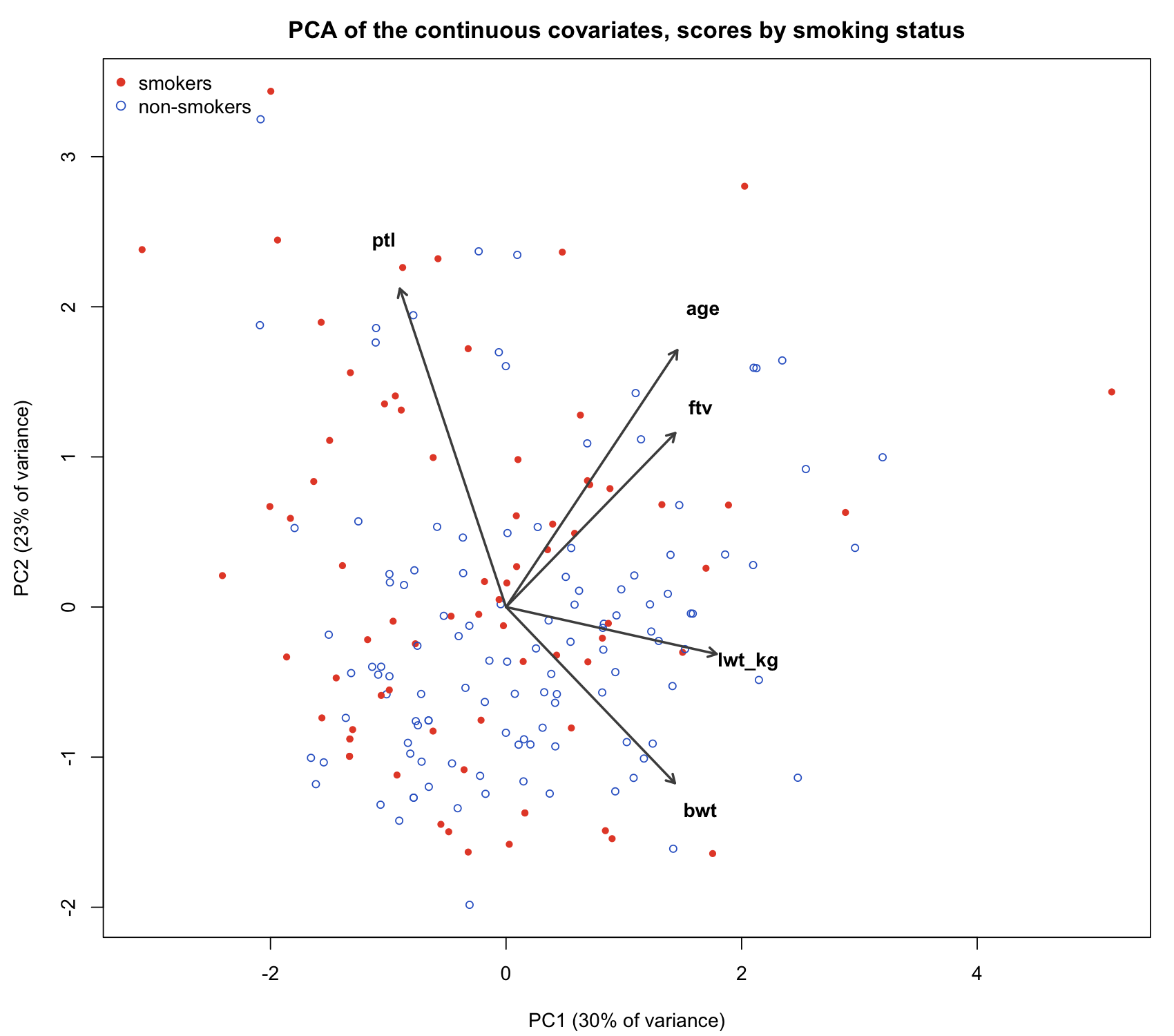
Before testing anything multivariate it is worth seeing how the continuous measurements co-vary. PCA on the standardised columns age, maternal weight, birth weight, previous premature labours and first-trimester visits.
cv <- bw[, c("age", "lwt_kg", "bwt", "ptl", "ftv")]
pc <- prcomp(cv, scale. = TRUE)
par(mar = c(4.2, 4.4, 2.5, 1))
plot(pc$x[, 1], pc$x[, 2], pch = ifelse(bw$smoke == "yes", 16, 1), cex = 0.8,
     col = ifelse(bw$smoke == "yes", rgb(0.9, 0.3, 0.2), rgb(0.2, 0.4, 0.8)),
     xlab = sprintf("PC1 (%.0f%% of variance)", 100 * summary(pc)$importance[2, 1]),
     ylab = sprintf("PC2 (%.0f%% of variance)", 100 * summary(pc)$importance[2, 2]),
     main = "PCA of the continuous covariates, scores by smoking status")
sc <- 3.2
arrows(0, 0, sc * pc$rotation[, 1], sc * pc$rotation[, 2], length = 0.08, lwd = 2, col = "grey30")
text(sc * 1.15 * pc$rotation[, 1], sc * 1.15 * pc$rotation[, 2], rownames(pc$rotation), font = 2)
legend("topleft", c("smokers", "non-smokers"), pch = c(16, 1), col = c(rgb(0.9, 0.3, 0.2), rgb(0.2, 0.4, 0.8)), bty = "n")
print(summary(pc))
cat("\nloadings:\n"); print(round(pc$rotation, 3))
cat("\ncorrelation matrix:\n"); print(round(cor(cv), 3))
Importance of components:
                          PC1    PC2    PC3    PC4    PC5
Standard deviation     1.2161 1.0676 0.9369 0.8906 0.8428
Proportion of Variance 0.2958 0.2280 0.1756 0.1586 0.1421
Cumulative Proportion  0.2958 0.5237 0.6993 0.8579 1.0000

loadings:
          PC1    PC2    PC3    PC4    PC5
age     0.454  0.535 -0.220 -0.037 -0.677
lwt_kg  0.559 -0.098 -0.144 -0.714  0.384
bwt     0.448 -0.367 -0.540  0.592  0.154
ptl    -0.282  0.663 -0.488  0.051  0.491
ftv     0.449  0.362  0.634  0.368  0.361

correlation matrix:
         age lwt_kg    bwt    ptl    ftv
age    1.000  0.180  0.090  0.072  0.215
lwt_kg 0.180  1.000  0.186 -0.140  0.141
bwt    0.090  0.186  1.000 -0.155  0.058
ptl    0.072 -0.140 -0.155  1.000 -0.044
ftv    0.215  0.141  0.058 -0.044  1.000
The correlations are all small; the first component carries 30 percent of the variance and five would be needed for all of it, so these covariates are close to independent and PCA buys no dimension reduction. That is itself informative: the smoking groups do not separate along any direction of the covariate space, so the adjustment in the regressions is not fighting collinearity, and on these continuous measures the two groups are well balanced (smokers are a year younger and a kilogram lighter on average, neither of which matters). The imbalance that drove the adjustment is in race, which is categorical and not part of this picture.
Hotelling’s T-squared: smokers versus non-smokers on three outcomes at once
Suppose I compare smokers and non-smokers on birth weight, maternal weight and age simultaneously. Three separate \(t\)-tests at the 5 percent level have a family-wise false-positive rate approaching 14 percent if independent. Hotelling’s \(T^2\) tests the single hypothesis that the mean vectors are equal:
\begin{equation} T^2 = \frac{n_1 n_2}{n_1 + n_2}\, (\bar{\mathbf{y}}_1 - \bar{\mathbf{y}}_2)^\top S_p^{-1} (\bar{\mathbf{y}}_1 - \bar{\mathbf{y}}_2), \qquad \frac{n_1 + n_2 - p - 1}{p\,(n_1 + n_2 - 2)}\, T^2 \sim F_{p,\; n_1 + n_2 - p - 1}, \end{equation}
with \(S_p\) the pooled covariance. It is a Wald statistic: the squared Mahalanobis distance between the two mean vectors, in the metric of their estimated covariance.
Y  <- as.matrix(bw[, c("bwt", "lwt_kg", "age")]); g <- bw$smoke
Y1 <- Y[g == "yes", ]; Y2 <- Y[g == "no", ]
n1 <- nrow(Y1); n2 <- nrow(Y2); p <- ncol(Y)
d  <- colMeans(Y1) - colMeans(Y2)
Sp <- ((n1 - 1) * cov(Y1) + (n2 - 1) * cov(Y2)) / (n1 + n2 - 2)
T2 <- drop(t(d) %*% solve(Sp * (1 / n1 + 1 / n2)) %*% d)
Fstat <- T2 * (n1 + n2 - p - 1) / (p * (n1 + n2 - 2))
cat("mean differences (smokers - non-smokers):", round(d, 2), "\n")
cat("Hotelling T2 =", round(T2, 3), "  F =", round(Fstat, 3), " on", p, "and", n1 + n2 - p - 1,
    "df;  p =", round(pf(Fstat, p, n1 + n2 - p - 1, lower.tail = FALSE), 4), "\n")
cat("Mahalanobis distance between group means:", round(sqrt(mahalanobis(colMeans(Y1), colMeans(Y2), Sp)), 3), "\n\n")
print(summary(manova(Y ~ g), test = "Hotelling-Lawley"))
cat("\nunivariate two-sample t-tests, p-values:\n")
pv <- sapply(1:p, function(j) t.test(Y1[, j], Y2[, j], var.equal = TRUE)$p.value)
pv_tab <- rbind(raw = pv, bonferroni = pmin(1, p * pv)); colnames(pv_tab) <- colnames(Y)
print(round(pv_tab, 4))
mean differences (smokers - non-smokers): -283.78 -1.25 -0.48
Hotelling T2 = 7.192   F = 2.372  on 3 and 185 df;  p = 0.0719
Mahalanobis distance between group means: 0.4

           Df Hotelling-Lawley approx F num Df den Df Pr(>F)
g           1         0.038458   2.3716      3    185 0.0719 .
Residuals 187
---
Signif. codes:  0 ‘***’ 0.001 ‘**’ 0.01 ‘*’ 0.05 ‘.’ 0.1 ‘ ’ 1

univariate two-sample t-tests, p-values:
              bwt lwt_kg    age
raw        0.0087 0.5461 0.5446
bonferroni 0.0260 1.0000 1.0000
The joint test does not reject at 5 percent (\(p = 0.07\)) even though the univariate test on birth weight alone has \(p = 0.009\). That is not a contradiction. The multivariate test spends its power over all three dimensions, and two of them (maternal weight and age) show nothing, so the signal in birth weight is diluted. Bonferroni on the three univariate tests still rejects for birth weight (\(p = 0.026\)). The honest summary is that the groups differ in birth weight and not detectably in the other two; the multivariate test is what protects that statement from being the product of a search over outcomes, and the price of that protection is sensitivity when the effect is concentrated in one coordinate.
What the evidence does and does not support
What these three datasets support, with the models above:
- In the Baystate births, maternal smoking is associated with a mean birth weight about 350 g lower (95 percent interval roughly 140 to 560 g) and with about 2.5 times the odds of low birth weight (1.15 to 5.5), after adjusting for age, maternal weight, race, hypertension, uterine irritability and prior premature labour. Wald, likelihood-ratio and score tests agree; sandwich standard errors do not change the picture; a Bayesian analysis with weakly informative priors gives practically the same intervals and puts the probability of a material effect at 0.9 or better under the thresholds I chose.
- In the Ille-et-Vilaine case-control study, each step up the tobacco scale multiplies the odds of oesophageal cancer by about 1.5 (1.3 to 1.9), adjusting for age and alcohol, and a single log-linear dose term fits as well as a free four-level factor.
- In Whickham, the apparent survival advantage of smokers reverses on adjustment for age: the age-adjusted odds of surviving twenty years are about 35 percent lower for smokers (odds ratio 0.65, 0.46 to 0.92).
What they do not support:
- A causal effect size. Every estimate is conditional on the recorded covariates, and the Whickham data demonstrate how one omitted variable can flip a sign. Smoking in pregnancy is correlated with socio-economic position, nutrition, alcohol and prenatal care, none of which
birthwtrecords beyond crude proxies. The causal conclusion that smoking harms is supported by a much larger literature, including quasi-experimental and mechanistic work; these datasets are consistent with it, and alone they would not establish it. - Precision beyond what 189 births allow. The odds-ratio interval for smoking runs from 1.15 to 5.5; “two and a half times the odds” is a point estimate with a wide tail. The sparse
hteffect in particular should be read from its profile interval, not its Wald interval. - Generalisation to other populations or decades. The birth data are from one American hospital in 1986, the cancer data from one French department in the 1970s, the survey from one English town. The direction of every effect matches what has been found elsewhere, which is the real reason to believe them; the magnitudes belong to their settings.
The honest statement is that the evidence here is consistent, in direction and in rough magnitude, with harm from smoking in three different outcomes and three different designs, and that the strength of that statement comes from the agreement across designs rather than from any one \(p\)-value on this page.
References
- Appleton, D. R., French, J. M. and Vanderpump, M. P. J. (1996). Ignoring a covariate: an example of Simpson’s paradox. The American Statistician, 50(4), 340-341.
- Breslow, N. E. and Day, N. E. (1980). Statistical Methods in Cancer Research, Volume 1: The Analysis of Case-Control Studies. IARC Scientific Publications No. 32, Lyon. (Source of the
esophdata.) - Gelman, A., Jakulin, A., Pittau, M. G. and Su, Y.-S. (2008). A weakly informative default prior distribution for logistic and other regression models. Annals of Applied Statistics, 2(4), 1360-1383.
- Hauck, W. W. and Donner, A. (1977). Wald’s test as applied to hypotheses in logit analysis. Journal of the American Statistical Association, 72(360), 851-853.
- Hosmer, D. W. and Lemeshow, S. (1989). Applied Logistic Regression. Wiley, New York. (Source of the
birthwtdata, via Venables and Ripley’sMASS.) - Venables, W. N. and Ripley, B. D. (2002). Modern Applied Statistics with S, 4th edition. Springer, New York.
- Zeileis, A. (2006). Object-oriented computation of sandwich estimators. Journal of Statistical Software, 16(9), 1-16.
Backlinks (1)
1. Blog /blog/
welcome
this page is for my non-technical ramblings.

“If I had a world of my own, everything would be nonsense.” —The Hatter
Comments