chapter 3: improving the way neural networks learn
3.1 the cross entropy function
- we often learn fastest when we're badly wrong about something
- the cross-entropy cost function is always negative (which is something you desire for a cost function)
- note here that at a = 1, you'll get
nan. we handle this in the code below. - this cost tends towards zero as the neuron gets better at computing the desired output y
- it also punishes bad guesses more harshly.
- the cross-entropy is nearly always the better choice, provided the output neurons are sigmoid neurons
- if the output neurons however are linear neurons, then the quadratic cost will not cause learning slowdown. you may use it.
- to find the learning rate \(\eta\) for log-reg, you can divide that of the lin-reg by 6.
- ch1 = 95.42 accuracy
-
100 hidden neurons \(\implies\) 96.82 percent.
- eliminated one in fourteen errors; pretty good!
- neuron saturation is an important problem in neural nets.
-
cross-entropy is a measure of surprise
- ch5 Cover & Thomas
- a softmax output layer with log-likelihood cost is quite similar to a sigmoid output layer with cross-entropy cost.
- softmax plus log-likelihood is worth using whenever you want to interpret the output activations as probabilities.
3.2 overfitting and regularisation
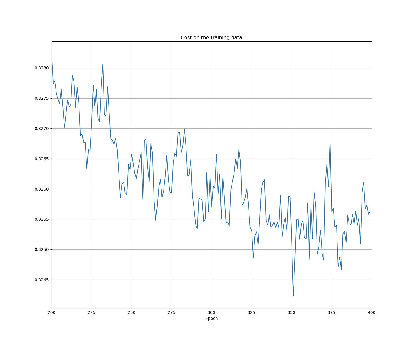
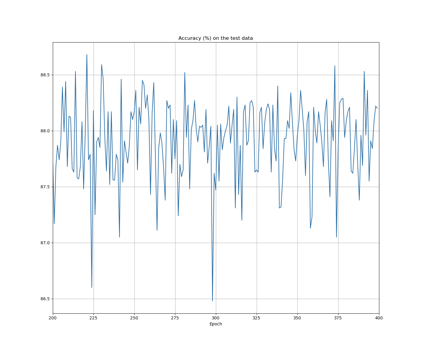
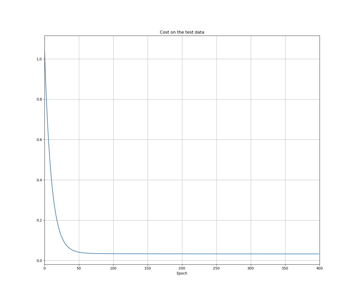
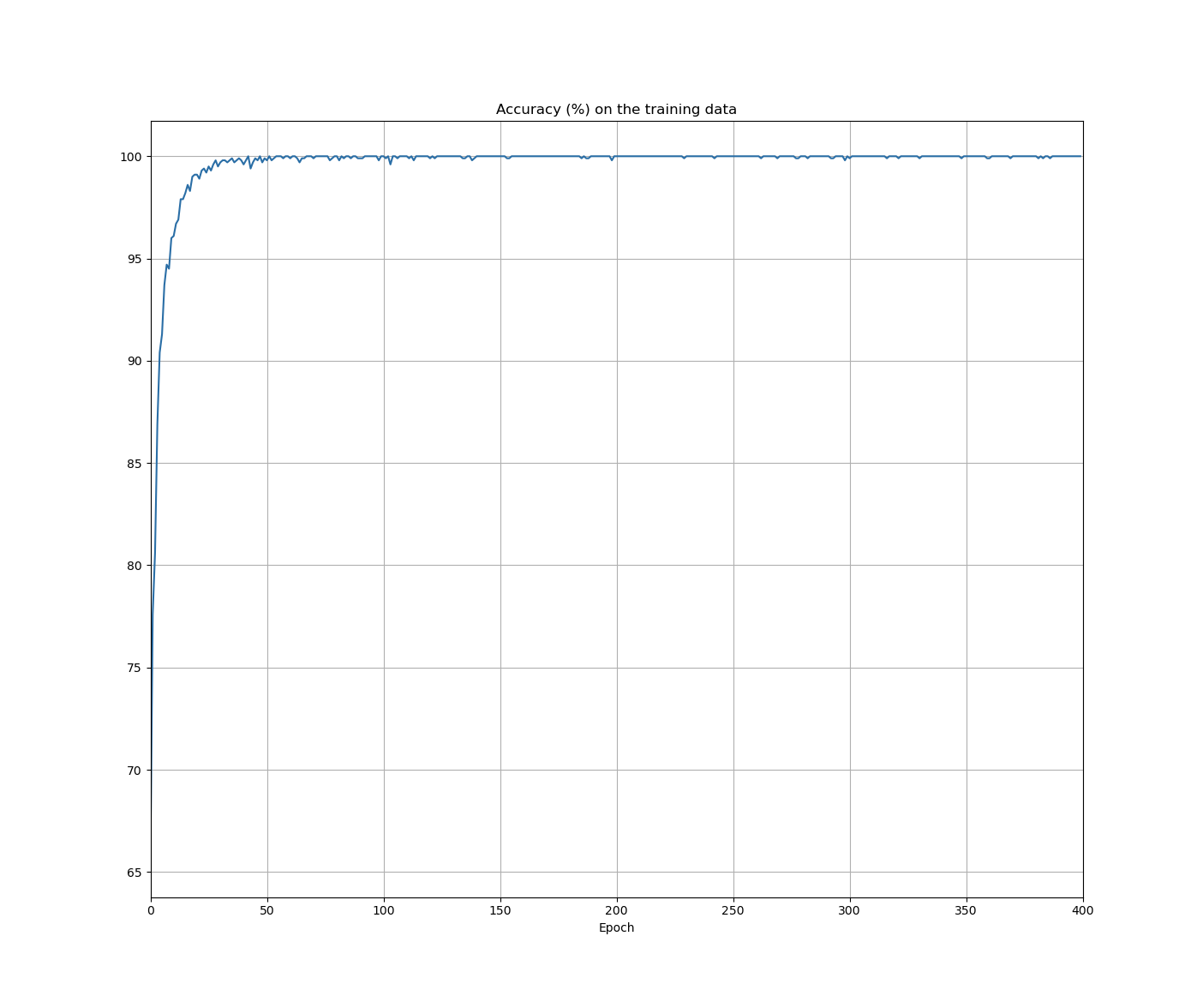
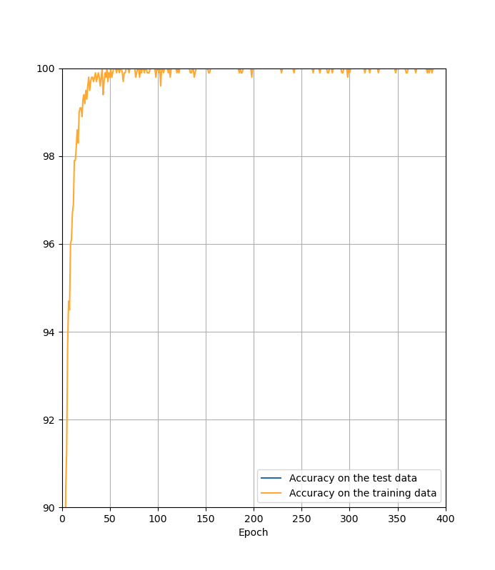
- the cost on the test data is no more than a proxy for classifiaction accuracy
-
once the classification accuracy on the validation_data has saturated, we stop training
- this strategy is called early stopping
- hold out method
- one of the best ways of reducing overfitting is to increase the size of the training data ⊕
- regularisation term doesn't include the biases
- intuitively, the effect of regularisation is to make it so the network prefers to learn small weights
- unregularised runs will occasionally get "stuck", apparently caught in local minima of the cost function
-
if the cost function is unregularised, then the length of the weight vector is likely to grow
- over time this weight vector can become very large and so will get stuck pointing in the same direction
-
"Occam's Razor" is a fallacy (I think)
- there is no a priori logical reason to prefer simple explanations over more complex explanations.
- it's an empirical reason that regularised neural nets usually generalise better than unregularised networks
- it has been conjectured that the dynamics of gradient descent learning in multilayer nets has a 'self-regularisation' effect
-
large biases make it easier for neurons to saturate
- we don't usually include bias terms when regularising
- L1 regularisation shrinks the weights by a constant amount toward 0
- in L2 regularisation, the weights shrink by an amount proportional to \(w\)
-
i.e. when \(|w|\) is small, L1 shrinks the weights more than L2, and when it is large L2 shrinks it harder than L1
- the net effect is L1 concentrates the weights into a select few high-importance connections
- dropout is like training different neural networks
- you can also translate and skew the data to generate more samples (and thus reduce your overfitting)
3.3 weight initialisation
-
just divide the standard deviation by \(\sqrt{n_{\text{in}}}\)
- it will slow down saturation
3.4 handwriting recognition revisited: the code
-
the cost plays two different roles in the network:
- a measure of how well an output activation,
a, matches the desired outputy - the derivative of this cost function used to update parameters
- a measure of how well an output activation,
Epoch 29 training complete Cost on training data: 0.1337562096961126 Accuracy on training data: 48414 / 50000 Cost on evaluation data: 0.6687826521607004 Accuracy on evaluation data: 9595 / 10000
code
"""network2.py
~~~~~~~~~~~~~~
An improved version of network.py, implementing the stochastic
gradient descent learning algorithm for a feedforward neural network.
Improvements include the addition of the cross-entropy cost function,
regularisation, and better initialisation of network weights. Note
that Nielsen has focessed on making the code simple, easily readable, and easily modifiable. It is _not_ optimised, and omits many desirable features.
"""
#### Libraries
# Standard Library
import json
import random
import sys
# Third Party Libraries
import numpy as np

#### Define the quadratic and cross-entropy cost functions.

class QuadraticCost(object):

  @staticmethod
  def fn(a, y):
    """Return the cost associated with an output 'a' and desired output 'y'.
    """
    return 0.5*np.linalg.norm(a-y)**2

  @staticmethod
  def delta(z, a, y):
    """Return the error delta from the output layer
    """
    return (a-y)*sigmoid_prime(z)


class CrossEntropyCost(object):
  @staticmethod
  def fn(a,y):
    return np.sum(np.nan_to_num(-y*np.log(a)-(1-y)*np.log(1-a)))

  @staticmethod
  def delta(z,a,y):
    return (a-y)

class Network(object):

  """i think it is important to write docstrings for code that other people
  will see.
  """
  def __init__(self, sizes, cost=CrossEntropyCost):
    self.num_layers = len(sizes)
    self.sizes = sizes
    self.default_weight_initialiser()
    self.cost = cost

  def default_weight_initialiser(self):
    """
    init each weight with mean 0 and standard dev = 1 over the sequare root

    of the number of weights connecting to the same neuron.

    init each bias using a gaussian dist with mean 0 and std dev = 1.
    no biases for the input layer
    """

    self.biases = [np.random.randn(y, 1) for y in self.sizes[1:]]
    self.weights = [np.random.randn(y, x)/np.sqrt(x)
      for x, y in
      zip(self.sizes[:-1], self.sizes[1:])]

  def large_weight_initialiser(self):
    """same as above, but with unnormalised weights."""
    self.biases = [np.random.randn(y, 1) for y in self.sizes[1:]]
    self.weights = [np.random.randn(y, x)
      for x, y in
      zip(self.sizes[:-1], self.sizes[1:])]

  def feedforward(self, a):
    """return the output of the network if 'a' is input"""
    for b, w in zip(self.biases, self.weights):
      a = sigmoid(np.dot(w, a)+b)
    return a

  def SGD(self, training_data, epochs, mini_batch_size, eta, lmbda = 0.0,
          evaluation_data=None, monitor_evaluation_cost=False,
          monitor_evaluation_accuracy=False, monitor_training_cost=False,
          monitor_training_accuracy=False):
    if evaluation_data:
      n_data = len(evaluation_data)
    n = len(training_data)
    evaluation_cost, evaluation_accuracy = [], []
    training_cost, training_accuracy = [], []
    for j in range(epochs):
      random.shuffle(training_data)
      mini_batches = [
        training_data[k:k+mini_batch_size]
        for k in range(0,n,mini_batch_size)]
      for mini_batch in mini_batches:
        self.update_mini_batch(mini_batch, eta, lmbda, len(training_data))
      print("Epoch %s training complete" % j)
      if monitor_training_cost:
        cost = self.total_cost(training_data, lmbda)
        training_cost.append(cost)
        print("Cost on training data: {}".format(cost))
      if monitor_training_accuracy:
        accuracy = self.accuracy(training_data, convert=True)
        training_accuracy.append(accuracy)
        print("Accuracy on training data: {} / {}".format(accuracy, n))
      if monitor_evaluation_cost:
        cost = self.total_cost(evaluation_data, lmbda, convert=True)
        evaluation_cost.append(cost)
        print("Cost on evaluation data: {}".format(cost))
      if monitor_evaluation_accuracy:
        accuracy = self.accuracy(evaluation_data)
        evaluation_accuracy.append(accuracy)
        print("Accuracy on evaluation data: {} / {}".format(self.accuracy(evaluation_data), n_data))
    return evaluation_cost, evaluation_accuracy, training_cost, training_accuracy

  def update_mini_batch(self, mini_batch, eta, lmbda, n):
    nabla_b = [np.zeros(b.shape) for b in self.biases]
    nabla_w = [np.zeros(w.shape) for w in self.weights]
    for x, y in mini_batch:
      delta_nabla_b, delta_nabla_w = self.backprop(x, y)
      nabla_b = [nb+dnb for nb, dnb in zip(nabla_b, delta_nabla_b)]
      nabla_w = [nw+dnw for nw, dnw in zip(nabla_w, delta_nabla_w)]
    self.weights = [(1-eta*(lmbda/n))*w-(eta/len(mini_batch))*nw
                    for w, nw in zip(self.weights, nabla_w)]
    self.biases = [b - (eta/len(mini_batch))*nb
                   for b, nb in zip(self.biases, nabla_b)]

  def backprop(self, x, y):
    """Return a tuple ''(nabla_b, nabla_w)'' representing the gradient for the cost function C_x. ''nabla_b'' and ''nabla_w'' are layer-by-layer lists of numpy arrays, similar to ''self.biases'' and ''self.weights''."""
    nabla_b = [np.zeros(b.shape) for b in self.biases]
    nabla_w = [np.zeros(w.shape) for w in self.weights]
    # feedforward
    activation = x
    activations = [x] # list to store all the activations, layer by layer
    zs = [] # list to store all the z vectors, layer by layer
    for b, w in zip(self.biases, self.weights):
      z = np.dot(w, activation) + b
      zs.append(z)
      activation = sigmoid(z)
      activations.append(activation)
    # backward pass
    delta = (self.cost).delta(zs[-1], activations[-1],y)
    nabla_b[-1] = delta
    nabla_w[-1] = np.dot(delta, activations[-2].transpose())
    for l in range(2, self.num_layers):
      z = zs[-l]
      sp = sigmoid_prime(z)
      delta = np.dot(self.weights[-l+1].transpose(),delta) * sp
      nabla_b[-l] = delta
      nabla_w[-l] = np.dot(delta, activations[-l-1].transpose())
    return (nabla_b, nabla_w)


  def accuracy(self, data, convert=False):
    """returns the number of inputs in ``data`` for which the nueral network
    outputs the correct result
    """
    if convert:
      results = [(np.argmax(self.feedforward(x)),np.argmax(y)) for (x, y) in data]
    else:
      results = [(np.argmax(self.feedforward(x)),y) for (x,y) in data]
    return sum(int(x==y) for (x,y) in results)

  def total_cost(self, data, lmbda, convert=False):
    cost =  0.0
    for x, y in data:
      a = self.feedforward(x)
    if convert:
      y = vectorised_result(y)
    cost += self.cost.fn(a,y)/len(data)
    cost += 0.5*(lmbda/len(data))*sum(np.linalg.norm(w)**2 for w in self.weights)
    return cost


  def save(self, filename):
    """save the neural net to file ``filename``"""
    data = {"sizes": self.sizes,
            "weights": [w.tolist() for w in self.weights],
            "biases": [b.tolist() for b in self.biases],
            "cost": str(self.cost.__name__)}
    f = open(filename, "w")
    json.dump(data, f)
    f.close()

def load(filename):
  """returns an instance of the network"""
  f = open(filename, "r")
  data = json.load(f)
  f.close()
  cost = getattr(sys.modules[__name__], data["cost"])
  net = Network(data["sizes"], cost=cost)
  net.weights = [np.array(w) for w in data["weights"]]
  net.biases = [np.array(b) for b in data["biases"]]
  return net

def vectorised_result(j):
  """is the e_i vector"""
  e = np.zeros((10,1))
  e[j] = 1.0
  return e

def sigmoid(z):
  return 1.0/(1.0+np.exp(-z))

def sigmoid_prime(z):
return sigmoid(z)*(1-sigmoid(z))3.5 how to choose a neural network's hyper-parameters
- it's easy to feel lost in hyper-parameter space
- it damages your confidence
- maybe you should quit your job and take up beekeeping
-
the way to go is to strip the problem down. get rid of all the training and validation images except images which are 0s and 1s
- then try to train a network to distinguish between the two.
- enables much more rapid experimentation
- as with many things in life, getting started can be the hardest thing to do.
- it's best to use a large learning rate that causes the weights to change quickly. later, we can reduce the learning rate
- a common technique is grid-search, which systematically searches through a grid in hyper-parameter space.
- books are never finished, only abandoned.
3.6 other techniques
- Hessian techniques can converge on a minimum in fewer steps, but are computationally more demanding
- conjugate gradient descent
- Nesterov's accelerated gradient technique
tanhis just a rescaled version of the sigmoid function
- explore boldly, as opposed to being rigorously correct.