From Convolution to CNNs
Hand-designed features (colour histograms, SIFT, HOG) followed by a trained classifier was the recipe for image recognition until about 2012. A convolutional neural network learns both halves at once, straight from the pixels. This page builds one from the bottom: why the obvious learned classifiers fail on images, what a convolutional layer does instead, the two formulas that size every layer, pooling and receptive fields, what the filters actually learn, and why very deep networks only train once you give them residual connections. 𐃏
The training side (backpropagation, optimisers, augmentation, transfer learning) is on the Backpropagation and Optimisers pages, and regularisation and initialisation in practice are in Improving the Way Neural Networks Learn. Convolution as a filtering operation, and its frequency-domain view, is on the Seeing in Frequency page.
why a linear classifier and an MLP struggle
one template per class
Flatten an image into \(\mathbf x \in \mathbb R^D\). For a \(32\times32\) colour image, \(D = 32\cdot32\cdot3 = 3072\).
For \(C\) classes, compute scores \(\mathbf z = \mathbf W\mathbf x + \mathbf b\) with \(\mathbf W \in \mathbb R^{C\times D}\), \(\mathbf b \in \mathbb R^C\), and predict \(\hat y = \arg\max_j z_j\).
Row \(j\) of \(\mathbf W\) is a template for class \(j\): the score is the dot product of the image with that template, a correlation evaluated at a single position. Ten classes on \(32\times32\times3\) images need \(10\cdot3072 + 10 = 30\,730\) parameters, and each class gets exactly one template. A cat facing left and a cat facing right have to share it.
The decision boundaries \(z_j = z_k\) are hyperplanes, so a class must occupy a half-space (more precisely, an intersection of half-spaces). Three toy problems in the plane show what that rules out.
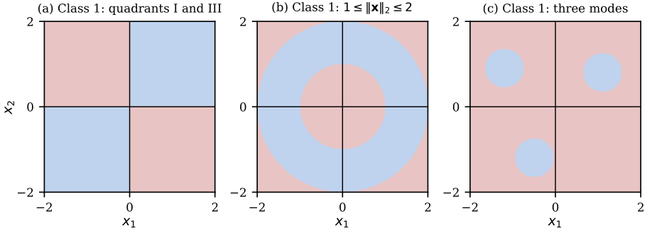
Three two-class problems no linear classifier can solve: (a) the quadrant (XOR) pattern, (b) an annulus, (c) a class made of three separate modes. Class 1 blue, class 2 red.
No \(\mathbf w \in \mathbb R^2\), \(b \in \mathbb R\) satisfy \(\mathbf w^\top\mathbf x + b > 0\) at \((1,1)\) and \((-1,-1)\) while \(\mathbf w^\top\mathbf x + b < 0\) at \((1,-1)\) and \((-1,1)\).
Hand-made features can rescue a particular case (\(x_1x_2\) separates the quadrants, \(r^2 = x_1^2 + x_2^2\) separates the annulus), but each fix needs you to know the shape of the answer in advance. The point of a neural network is to learn such features.
hidden layers, and why they need a non-linearity
A fully connected (FC) layer maps \(\mathbf a \in \mathbb R^n\) to \(\mathbf W\mathbf a + \mathbf b \in \mathbb R^m\), with one weight per input–output pair. A multilayer perceptron alternates FC layers with an elementwise activation \(g\), usually the ReLU \(g(z) = \max(0, z)\): \[ \mathbf z = \mathbf W^{(2)}\max\bigl(0,\ \mathbf W^{(1)}\mathbf x + \mathbf b^{(1)}\bigr) + \mathbf b^{(2)} . \]
The activation does all the work.
If \(g\) is the identity (or any affine map), an \(L\)-layer network computes \(\mathbf z = \mathbf W’\mathbf x + \mathbf b’\) with \(\mathbf W’ = \mathbf W^{(L)}\cdots\mathbf W^{(1)}\): it is a linear classifier, however many layers it has.
With the ReLU in place, a single hidden layer of four units solves the quadrant problem.
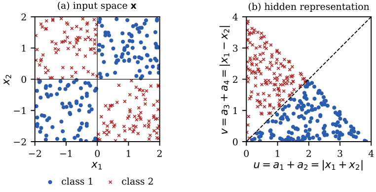
The quadrant problem (a) and its image in the hidden layer (b). The hidden layer bends the plane so that a single line, \(u = v\), separates the classes.
That picture is the whole idea of deep learning in miniature: the hidden layers transform the input until the last layer, which is just a linear classifier, can do its job.
why not just use an MLP on pixels?
Two reasons, and they are the two things a convolutional layer fixes.
- Parameter count
- Every hidden unit sees every pixel. A \(224\times224\times3\) input into 4096 hidden units needs \(150\,528\cdot4096 + 4096 = 616\,566\,784\) parameters in the first layer alone.
- No notion of neighbourhood
- Flattening throws the grid away. A stroke detector learned in the top-left corner has to be learned again, with different weights, at every other position, and a one-pixel shift of the input can change the output arbitrarily.
FC layers are the right tool on short feature vectors, which is exactly where a CNN uses them: at the end, after the convolutional layers have done the spatial work.
proofs
Suppose such \(\mathbf w = (w_1, w_2)\) and \(b\) exist. Adding the two class-1 inequalities, \((w_1 + w_2 + b) + (-w_1 - w_2 + b) > 0\), so \(2b > 0\). Adding the two class-2 inequalities, \((w_1 - w_2 + b) + (-w_1 + w_2 + b) < 0\), so \(2b < 0\). Contradiction. With two scores, \(z_1 - z_2\) is again of the form \(\mathbf w^\top\mathbf x + b\), so the same argument applies.
Induction on \(L\). One layer is \(\mathbf W^{(1)}\mathbf x + \mathbf b^{(1)}\). If the first \(L-1\) layers compute \(\mathbf u = \mathbf V\mathbf x + \mathbf c\), then \[ \mathbf z = \mathbf W^{(L)}(\mathbf V\mathbf x + \mathbf c) + \mathbf b^{(L)} = (\mathbf W^{(L)}\mathbf V)\mathbf x + (\mathbf W^{(L)}\mathbf c + \mathbf b^{(L)}), \] which is affine in \(\mathbf x\). An affine activation \(g(z) = \alpha z + \beta\) only rescales and shifts each layer, with the same conclusion.
the convolutional layer
intuition: small, shared, local
Keep the image as a grid. Let each output unit look only at a small \(k\times k\) neighbourhood (local connectivity), and use the same weights at every position (parameter sharing). That is exactly a filter slid over the image, as in classical spatial filtering, except that the filter’s weights are now learned. A stroke detector learned at one position automatically works at every position, and the parameter count no longer depends on the image size.
The input is a stack of \(c_{\text{in}}\) feature maps \(A(x, y, c)\). The layer has \(c_{\text{out}}\) filters; filter \(m\) is a \(k\times k\times c_{\text{in}}\) block of weights \(W_m\) with a bias \(b_m\), and produces the feature map \[ Z_m(x, y) = b_m + \sum_{c=1}^{c_{\text{in}}}\sum_{i,j} W_m(i, j, c)\,A(x + i,\ y + j,\ c). \] The \(c_{\text{out}}\) maps are stacked into the output volume, and an activation (ReLU) is applied entrywise. Besides \(c_{\text{in}}\), \(c_{\text{out}}\) and \(k\), the layer is fixed by its stride \(s\), padding \(p\) (and padding mode) and dilation \(d\).
Three facts that trip people up:
- It is a correlation
- The formula has \(A(x + i, y + j)\), not \(A(x - i, y - j)\). Deep-learning “convolution” is correlation. Because the weights are learned it makes no difference: training would simply learn the flipped kernel.
- A filter spans the full input depth
- On an RGB input a \(5\times5\) filter is really \(5\times5\times3\). Its three slices are summed into one feature map, so the output depth is the number of filters, whatever \(c_{\text{in}}\) is.
- The weights are not designed
- Classical kernels (Sobel, Laplacian) are a useful mental model for what a filter might learn, nothing more.
Input volume \(X\) (\(n_{\text{in}}\times n_{\text{in}}\times c_{\text{in}}\)); filters \(W_1, \dots, W_{c_{\text{out}}}\); biases; stride \(s\), padding \(p\), dilation \(d\).
- Pad \(X\) by \(p\) pixels on every side (zeros by default).
- For each filter \(c = 1, \dots, c_{\text{out}}\) and each output position \((i, j)\): take the patch whose top-left tap is at \((is, js)\), with taps \(d\) pixels apart; set \(Y(i, j, c)\) to the dot product of \(W_c\) with that patch, plus \(b_c\).
- Apply the ReLU to every entry of \(Y\) and return it.
Cost: \(n_{\text{out}}^2\, c_{\text{out}}\, k^2 c_{\text{in}}\) multiply–adds.
Stride 1, no padding, so the output is \(3\times3\).
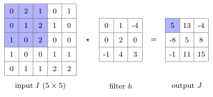
Single-channel convolution (as correlation). The shaded patch times the filter, entry by entry and summed, gives the shaded output.
Top-left output, row by row of the patch against the filter: \[ (0\cdot0 + 2\cdot1 + 1\cdot(-4)) + (0\cdot0 + 1\cdot2 + 2\cdot0) + (1\cdot(-1) + 0\cdot4 + 2\cdot3) = -2 + 2 + 5 = 5 . \] One column to the right: \[ (0 + 1 + 0) + (0 + 4 + 0) + (0 + 8 + 0) = 13. \] The other seven positions give \[ J = \begin{pmatrix}5&13&-4\\-8&5&8\\-1&11&15\end{pmatrix}, \qquad \operatorname{ReLU}(J) = \begin{pmatrix}5&13&0\\0&5&8\\0&11&15\end{pmatrix}. \] The output is large where large pixels sit under the large positive taps (4, 3, 2) and negative where they sit under the \(-4\). ReLU keeps only the matches: the layer is a bank of learned template detectors, each run everywhere.
the volume picture
On a \(32\times32\times3\) image, one \(5\times5\times3\) filter gives one number \(\mathbf w^\top\mathbf x + b\) (a 75-dimensional dot product) per position, and sliding it over the \(28\times28\) positions where it fits gives one \(28\times28\) map. Six filters give six maps, stacked into a \(28\times28\times6\) output volume: a grid with a six-dimensional feature vector at every pixel. The next layer’s filters are then \(k\times k\times6\), and so on.
Here is one filter, a horizontal-derivative kernel standing in for a learned first-layer filter, run through a full conv, ReLU, pool block on a real photograph.
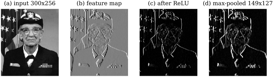
One filter through a CNN block: (b) the feature map is positive (light) on dark-to-bright vertical edges and negative (dark) on bright-to-dark ones; (c) ReLU zeroes the negative half, here 49.8% of the values; (d) 2-by-2 max pooling halves each side.
ReLU throws away the bright-to-dark edges entirely, which is one reason a layer has many filters: a second filter of the opposite sign picks them up.
output size and parameter counting
Two formulas carry almost every calculation about a CNN. Getting the size wrong is the commonest bug when building one, because the next layer’s input, and the length of the flattened vector entering the FC head, both follow from it.
the output-size formula
Count the positions where the filter fits. On a \(7\times7\) input with a \(3\times3\) filter and no padding, stride 1 gives 5 positions per side, stride 2 gives 3 (left edges at 0, 2, 4), and stride 3 gives 2: the next window, starting at column 6, would hang off the edge.
With input size \(n_{\text{in}}\), kernel size \(k\), stride \(s\), padding \(p\) per side and dilation \(d\), each spatial side of the output is \[ n_{\text{out}} = \left\lfloor \frac{n_{\text{in}} + 2p - d(k-1) - 1}{s} \right\rfloor + 1 . \] Height and width are computed separately. The output depth is \(c_{\text{out}}\) and depends on none of these.
The quantity \(k_{\text{eff}} = d(k-1) + 1\) is the span of a dilated filter, so with \(d = 1\) the formula is the familiar \((n_{\text{in}} + 2p - k)/s + 1\). The special cases worth knowing by heart:
- Valid (\(s = 1\), \(p = 0\))
- \(n_{\text{out}} = n_{\text{in}} - k + 1\): each layer eats \(k - 1\) pixels.
- Same (\(s = 1\), \(k\) odd, \(p = (k-1)/2\))
- \(n_{\text{out}} = n_{\text{in}}\). Hence \(3\times3\) with padding 1, \(5\times5\) with padding 2. An even \(k\) has no symmetric “same” padding, one reason kernels are odd.
- Strided
- Stride \(s\) divides the size by about \(s\). If \((n_{\text{in}} + 2p - k_{\text{eff}})/s\) is not an integer, the hyperparameters “do not fit”; PyTorch silently drops the leftover pixels, which is what the floor expresses.
| layer | arithmetic | output |
|---|---|---|
| \(7\times7\), \(k=3\), \(s=1\), \(p=1\) | \((7+2-3)/1+1\) | 7 |
| \(7\times7\), \(k=3\), \(s=3\) | \(\lfloor 4/3\rfloor + 1\) | 2 |
| \(7\times7\), \(k=3\), \(d=2\) | \(7 - 5 + 1\) | 3 |
| AlexNet conv1: 227, \(k=11\), \(s=4\) | \((227-11)/4+1\) | 55 |
The last row is why AlexNet’s input is really \(227\times227\): with 224, \((224 - 11)/4 + 1 = 54.25\) does not fit.
counting parameters
A layer with \(c_{\text{out}}\) filters of size \(k_h\times k_w\) on \(c_{\text{in}}\) input channels, one bias each, has \[ \#\text{params} = c_{\text{out}}\,(k_h k_w\, c_{\text{in}} + 1). \] It does not depend on the input size, the stride, the padding or the dilation.
Stride and padding change the output size, not the parameter count; a larger stride gives a smaller output, more padding a larger one. Those two distinctions are what exam questions test.
Map a \(32\times32\times3\) image to a \(28\times28\times6\) volume.
Convolutional, six \(5\times5\times3\) filters: \(6\,(75 + 1) = 456\) parameters.
Fully connected: each of the \(28\cdot28\cdot6 = 4704\) outputs connects to all 3072 inputs, so \(3072\cdot4704 + 4704 = 14\,455\,392\) parameters, about 31,700 times as many.
Local connectivity cuts each output’s inputs from 3072 to 75; sharing cuts the 4704 separate weight sets down to six.
Input \(227\times227\times3\); 96 kernels of \(11\times11\), stride 4, no padding. Output \(55\times55\times96\) (one map per kernel). Parameters \(96\,(11\cdot11\cdot3 + 1) = 96\cdot364 = 34\,944\).
That is 0.06% of AlexNet’s 62.4 million parameters. Its first FC layer (\(6\cdot6\cdot256 = 9216\) inputs to 4096 units) holds 37.8 million, 60% of the network. Convolutional layers are cheap in parameters and expensive in computation; FC layers are the reverse.
proofs
Work along one axis. The padded input has length \(L = n_{\text{in}} + 2p\), indexed \(0, \dots, L-1\). The dilated filter spans \(k_{\text{eff}} = d(k-1) + 1\) pixels (\(k - 1\) gaps of width \(d\), plus the first tap). Window \(i\) starts at \(is\) and ends at \(is + k_{\text{eff}} - 1\); it fits iff \(is + k_{\text{eff}} - 1 \le L - 1\), i.e. iff \(i \le (L - k_{\text{eff}})/s\). The number of integers \(i \ge 0\) satisfying this is \[ \left\lfloor \frac{L - k_{\text{eff}}}{s} \right\rfloor + 1 = \left\lfloor \frac{n_{\text{in}} + 2p - d(k-1) - 1}{s} \right\rfloor + 1 , \] and each fitting window produces one output pixel. (“Same” padding: with \(s = d = 1\) and \(2p = k - 1\), the numerator is \(n_{\text{in}} - 1\), so \(n_{\text{out}} = n_{\text{in}}\).)
A filter spans the full input depth, so it has \(k_h k_w c_{\text{in}}\) weights, plus one bias; there is one filter per output channel. The same filter is reused at every position, so the number of positions, and with it \(n_{\text{in}}\), \(s\), \(p\) and \(d\), never enters. A dilated filter has the same taps, only spread apart.
pooling
After convolution and ReLU the feature maps are still image-sized, and there are many of them. Pooling shrinks them.
Slide a \(k\times k\) window with stride \(s\) over each feature map separately and replace each window by its maximum (max pooling) or mean (average pooling). The usual \(k = s = 2\) halves height and width and keeps the number of channels. A pooling layer has no learnable parameters.
\(2\times2\) windows, stride 2: \[ F = \begin{pmatrix}3&2&0&0\\0&7&1&3\\5&2&3&0\\0&9&2&3\end{pmatrix} \quad\longmapsto\quad \text{max: } \begin{pmatrix}7&3\\9&3\end{pmatrix}, \qquad \text{average: } \begin{pmatrix}3&1\\4&2\end{pmatrix}. \] Top-left window \(\{3, 2, 0, 7\}\): maximum 7, mean 3. Bottom-left \(\{5, 2, 0, 9\}\): maximum 9, mean 4. A quarter of the values, the same number of channels.
Pooling detects nothing; the features are found by the convolution filters, and pooling only summarises each window. Max pooling says “the feature occurred somewhere in here”. That buys two things: later layers see a larger part of the image for the same kernel size, and a feature that moves by a pixel but stays inside its window produces the same pooled value. The insensitivity is only partial (a shift across a window boundary changes the output), but stacking pooling layers widens the range of shifts absorbed.
Pooling throws away where in each window the feature was, which hurts tasks that need exact positions: a label per pixel, a tight bounding box. Segmentation networks have to undo it with upsampling. Average pooling also dilutes a strong, small response with the zeros around it.
When to use what. Max pooling is the default inside a classification feature extractor. Average pooling suits smooth summaries, above all global average pooling, which averages each channel over the whole map just before the classifier. A strided convolution downsamples too, with learned weights instead of a fixed rule.
The head of the network is short. Flatten the last \(n\times n\times c\) maps into a vector of length \(n^2c\), pass it through one or more FC layers, and turn the final \(C\) scores into probabilities with the softmax, \[ p_j = \frac{e^{z_j}}{\sum_{k=1}^C e^{z_k}} , \] computed in practice as the softmax of \(\mathbf z - \max_k z_k\) (the same probabilities, with no overflow).
receptive fields
Why do small kernels suffice? Because what matters for a deep unit is how much of the input it can see, and every layer enlarges that.
The receptive field of a unit is the region of the input image whose pixels can affect its value. For layers with kernel sizes \(k_1, \dots, k_L\) and strides \(s_1, \dots, s_L\), its side length is \[ r_L = 1 + \sum_{l=1}^{L} (k_l - 1)\prod_{j=1}^{l-1} s_j . \] With every stride equal to 1 this is \(r_L = 1 + L(k-1)\): each \(3\times3\) layer adds 2.
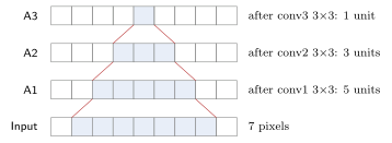
Receptive field of three stacked 3-by-3 convolutions (stride 1), along one axis. One unit at the top sees 3 units below it, 5 below that, and 7 input pixels.
Three stacked \(3\times3\) layers (stride 1) have the same \(7\times7\) receptive field as one \(7\times7\) layer. With \(C\) channels in and out of every layer, the single layer has \(49C^2\) weights and the stack \(27C^2\), and the stack applies three non-linearities instead of one.
For \(C = 64\): \(49\cdot64^2 = 200\,704\) weights against \(27\cdot64^2 = 110\,592\). The stack is deeper, more non-linear and 45% smaller. That one observation is VGG’s entire design.
Strides multiply in: after a stride-2 layer, every later \(3\times3\) kernel adds 4 input pixels instead of 2. This is how pooling and strided convolutions let a network see the whole image in a modest number of layers. Dilation is the other cheap way to grow the receptive field: a \(3\times3\) filter with \(d = 2\) spans \(k_{\text{eff}} = 5\) pixels with nine weights instead of 25. Its failure mode is that detail finer than the gap falls between the taps, and stacking layers with the same \(d\) leaves a regular grid of input pixels that never influence an output (gridding). Use it where you need context without downsampling, as in per-pixel labelling.
proofs
With no layers a unit is one pixel, \(r_0 = 1\). A unit in layer \(l\) reads \(k_l\) adjacent units of layer \(l-1\), i.e. \(k_l - 1\) more than one. Adjacent units of layer \(l-1\) are \(\prod_{j<l} s_j\) input pixels apart, because each earlier stride multiplies the spacing. So \(r_l = r_{l-1} + (k_l - 1)\prod_{j<l} s_j\), and summing from \(r_0 = 1\) gives the formula.
Receptive fields: \(1 + 3\cdot2 = 7\) and \(1 + 6 = 7\). One \(7\times7\) layer has \(C\) filters of \(7\cdot7\cdot C\) weights, \(49C^2\). One \(3\times3\) layer has \(9C^2\), three have \(27C^2\). Each layer ends in a ReLU.
a whole network: learned filters on Chinese-MNIST
Put the blocks together. A classic small digit network: two valid \(5\times5\) convolutions, each followed by \(2\times2\) max pooling, then flatten, an FC ReLU layer and a softmax.

A small CNN for 28-by-28 digits. Feature maps shrink in size and grow in number with depth; the FC head classifies the flattened vector.
On \(28\times28\times1\) input, sizes by the output-size formula: \(28 \to 24\) (conv) \(\to 12\) (pool) \(\to 8\) (conv) \(\to 4\) (pool), so the flattened vector has \(16n_2\) entries. With \(n_1 = 32\), \(n_2 = 64\), \(n_3 = 128\):
| layer | formula | parameters |
|---|---|---|
| conv 1 (1 to 32) | \(32(25 + 1)\) | 832 |
| conv 2 (32 to 64) | \(64(25\cdot32 + 1)\) | 51,264 |
| FC (1024 to 128) | \(128(1024 + 1)\) | 131,200 |
| output (128 to 10) | \(10(128 + 1)\) | 1,290 |
| total | 184,586 |
The first FC layer holds 71% of the parameters. The convolutions, which do all the feature extraction, hold under a third.
The same architecture with 6 and 16 filters, 64 hidden units and 15 outputs was trained from scratch on the \(64\times64\) Chinese-MNIST handwritten numerals (12,000 training images, 3000 test, four epochs of Adam). Shapes run \(64 \to 60 \to 30 \to 26 \to 13\), the parameter count is 176,667, and test accuracy reached 71.2%. Better accuracy needs longer training, but the interesting part is already visible in the first layer.
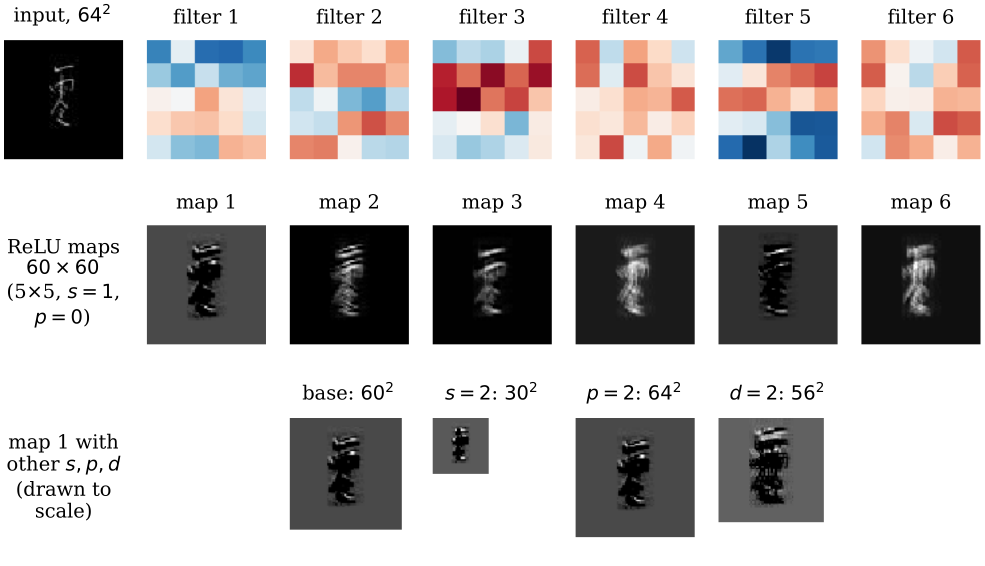
First layer of the trained network. Top: a test digit and the six learned 5-by-5 filters (red positive, blue negative). Middle: their ReLU activation maps (60 by 60). Bottom: map 1 recomputed with stride 2 (30 by 30), padding 2 (64 by 64) and dilation 2 (56 by 56), exactly as the output-size formula predicts.
The filters started as random noise and were shaped only by the class labels. Each has become a stroke or edge detector with a positive and a negative side, tuned to one orientation or polarity, which is what the first layer of almost every image CNN learns. Deeper layers combine these into corners and stroke junctions, then into parts of characters; the receptive-field arithmetic is what lets them.
why depth degrades
If small stacked kernels are good, more of them should be better. A deeper network contains a shallower one (the extra layers could just copy their input), so on the training set more depth should never hurt. In practice it does: a 56-layer plain CNN has higher training and test error than a 20-layer one.
Degradation is higher training error in a deeper plain network than in a shallower one. It is an optimisation failure, not overfitting: an overfitted model fits its training set well and generalises badly, whereas a degraded one cannot even fit its training set.
The cause is that plain layers find the identity map hard to learn, and gradients reaching early layers are products of many Jacobians, which shrink or blow up geometrically with depth. Batch normalisation helps but does not cure it.
Three small CNNs on 3000 Chinese-MNIST digits (\(32\times32\), 15 classes), six epochs, identical optimiser (SGD, learning rate 0.05, momentum 0.9). Each has a stride-2 stem, blocks of two \(3\times3\) convolutions with batch norm and 12 channels, two max pools, global average pooling and one FC layer. Training loss:
| network | epoch 1 | epoch 6 |
|---|---|---|
| plain, 8 layers (3 blocks) | 2.390 | 0.408 |
| plain, 22 layers (10 blocks) | 2.532 | 1.421 |
| residual, 22 layers | 2.304 | 0.446 |
The deeper plain network fits its own training data more than three times worse. That is degradation.
residual connections
ResNet’s fix starts from the observation above: a deeper model should be at least as good as a shallower one, because extra layers could be identities. So make the identity the default.
A residual block computes \[ \mathbf y = \operatorname{ReLU}\bigl(\mathcal F(\mathbf x) + \mathbf x\bigr), \] where \(\mathcal F\) is a small stack of layers (two \(3\times3\) convolutions with a ReLU between them in the basic block) and the identity shortcut carries \(\mathbf x\) around it unchanged. If \(\mathcal F\) changes the shape, the shortcut becomes a strided \(1\times1\) convolution (a projection) so the two terms can be added.
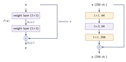
Left: the basic residual block. Right: the bottleneck block of ResNet-50 and deeper, which reduces the channels with a 1-by-1 convolution, works at 64 channels, and restores them.
If the best thing a block can do is nothing, it only has to drive \(\mathcal F\) to zero, which is easy. And the shortcut carries the gradient back undamped.
For \(\mathbf y = \mathbf x + \mathcal F(\mathbf x)\) and any loss \(\mathcal L\), \[ \frac{\partial\mathcal L}{\partial\mathbf x} = \frac{\partial\mathcal L}{\partial\mathbf y}\left(\mathbf I + \frac{\partial\mathcal F}{\partial\mathbf x}\right), \] so the gradient reaching \(\mathbf x\) always contains \(\partial\mathcal L/\partial\mathbf y\) itself, however small \(\partial\mathcal F/\partial\mathbf x\) is. Through a stack of blocks, \(\mathbf x_L = \mathbf x_l + \sum_{i=l}^{L-1}\mathcal F_i(\mathbf x_i)\).
Back to the experiment. Adding the shortcuts to the 22-layer network, and changing nothing else, brings its training loss from 1.421 down to 0.446, level with the shallow network.
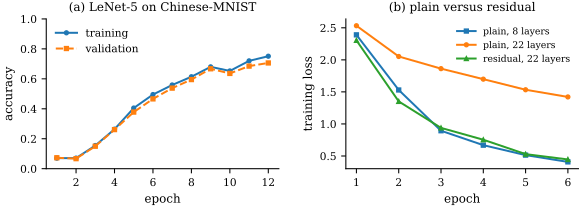
Small CNNs trained from scratch on Chinese-MNIST. (a) LeNet-5 training and validation accuracy, close together, so not yet overfitting. (b) Training loss: the 22-layer plain network degrades, the same network with identity shortcuts does not.
A second reading: unroll \(n\) residual blocks, each of which either passes through \(\mathcal F_i\) or skips it, and you get \(2^n\) paths of different lengths from input to output. A ResNet behaves like an ensemble of shallower networks.
The bottleneck block makes depth affordable. A basic block on 64 channels has \(2\cdot9\cdot64^2 = 73\,728\) weights. A bottleneck on 256 channels has \(256\cdot64 + 9\cdot64^2 + 64\cdot256 = 69\,632\): four times the channels for slightly fewer weights. A basic block on 256 channels would cost \(1\,179\,648\). That is why ResNet-50 costs about the same as ResNet-34 (3.8 against 3.6 GFLOPs) while being half again as deep.
Shortcuts cure degradation, not overfitting: a 152-layer ResNet trained from scratch on a few thousand images will still memorise them. On a small data set, either fine-tune a pretrained ResNet or use a shallow network. And the addition needs matching shapes, so every change of resolution or width costs a projection.
proofs
The chain rule on \(\mathbf y = \mathbf x + \mathcal F(\mathbf x)\) gives \(\partial\mathbf y/\partial\mathbf x = \mathbf I + \partial\mathcal F/\partial\mathbf x\); multiply by \(\partial\mathcal L/\partial\mathbf y\). For a stack, \(\mathbf x_{i+1} = \mathbf x_i + \mathcal F_i(\mathbf x_i)\), and summing over \(i = l, \dots, L-1\) telescopes. In a plain network the gradient is instead a product of \(L - l\) Jacobians, which shrinks or grows geometrically when they are consistently small or large.
the architecture line
Each architecture answers a failure of the one before it, and the ImageNet challenge (ILSVRC, 1000 classes) is where most of them were introduced.
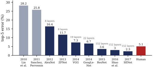
ILSVRC classification winners: top-5 error by year, with depth. The first two entries use hand-crafted features; every winner from AlexNet on is a CNN, and from 2015 they beat the 5.1% human reference.
- LeNet-5 (1998)
- Two \(5\times5\) convolution and subsampling stages, then three FC layers, tanh activations, trained by backpropagation on \(32\times32\) digits. About 61,700 weights, almost all in the FC layers. The template for everything after it.
- AlexNet (2012)
- Eight layers (five conv, three FC). The new ingredients were ReLU instead of saturating activations, dropout, data augmentation and training on two GPUs. It cut ImageNet top-5 error from 25.8% to 16.4%. Of its 62.4 million parameters, 94% sit in the FC layers.
- VGG (2014)
- Only \(3\times3\) convolutions with “same” padding, in five stages separated by \(2\times2\) pooling, channels doubling to 512. Depth buys the receptive field (three \(3\times3\) layers see \(7\times7\)). VGG-16 has 138 million parameters, 102.8 million of them in the first FC layer. Clean and heavy.
- GoogLeNet / Inception (2014)
- Goes wider instead of only deeper: each module runs \(1\times1\), \(3\times3\), \(5\times5\) convolutions and a pooling branch in parallel and concatenates them. Cheap \(1\times1\) convolutions shrink the channel count in front of the expensive branches, and global average pooling replaces the giant FC layer. 22 layers, 6.7% top-5.
- ResNet (2015)
- Identity shortcuts make 50, 101 and 152 layers trainable; bottleneck blocks keep them affordable. 3.6% top-5, below the human reference. Still the default backbone.
- EfficientNet (2019)
- Scales depth, width and input resolution together, \(d = \alpha^\phi\), \(w = \beta^\phi\), \(r = \gamma^\phi\) with \(\alpha\beta^2\gamma^2 \approx 2\), so each step of \(\phi\) doubles the FLOPs. EfficientNet-B7 matches GPipe’s 84.3% top-1 with 66 million parameters instead of 556 million.
- ViT (2021)
- Drops convolution: cut the image into \(16\times16\) patches, embed each as a token, and run a Transformer encoder with self-attention, so every patch can interact with every other from the first layer. See Visual Transformers.
Two side branches are worth a line each. SENet (2017) reweights the channels of a feature map from its global average, a cheap add-on to any block. DenseNet (2017) concatenates every earlier layer’s output instead of adding one shortcut, so channels grow by a fixed rate per layer.
Input \(28\times28\times192\); the \(5\times5\) branch should output 32 channels. Counting multiplications as positions \(\times\) output channels \(\times\) kernel volume:
Direct: \(28\cdot28\cdot32\cdot(25\cdot192) = 120\,422\,400\), with 153,600 weights.
With a \(1\times1\) reduction to 16 channels first: \(28\cdot28\cdot16\cdot192 = 2\,408\,448\) plus \(28\cdot28\cdot32\cdot(25\cdot16) = 10\,035\,200\), together \(12\,443\,648\), with 15,872 weights.
Ten times cheaper, same output shape. A \(1\times1\) convolution changes the channel count without changing the receptive field.
Why does ViT need so much more data? Inductive bias. A CNN builds in locality and translation equivariance, so it does not have to learn that neighbouring pixels are related or that a stroke means the same thing everywhere. A ViT has neither and must learn both from data, which pays off only with very large data sets or pretraining. Its attention also costs the square of the number of tokens: 197 tokens for a \(224\times224\) image give a \(197^2 = 38\,809\)-entry attention matrix per head and layer. ConvNeXt (2022) went the other way, modernising a ResNet step by step with ViT’s design choices (a non-overlapping “patchify” stem, large depthwise kernels, fewer activations and norms) while staying a pure CNN, and reached 82.0% against ResNet-50’s 78.8% at a similar budget, level with the Swin Transformer.
Start from a pretrained ResNet, or an EfficientNet when parameters or FLOPs are tight, and fine-tune it. VGG and AlexNet are mainly of historical and teaching value: their FC layers carry most of their parameters. Reach for a ViT when you have, or can borrow through pretraining, a very large data set. On a small data set trained from scratch, prefer a shallow network or a short residual one; depth without shortcuts degrades. And if your network ends in FC layers, it needs a fixed input size; global average pooling removes that constraint.
Worked PyTorch implementations of AlexNet, VGG and ResNet are in the modern CNNs chapter of Dive into Deep Learning. The residual-learning paper is He et al. (2015).
see also
- Computer Vision – the parent branch, whose image-processing section has convolution as a filter
- CNN from scratch – a convolutional network implemented by hand
- Object Detection and Semantic and Instance Segmentation – what these backbones are used for: boxes, then masks
- Seeing in Frequency – convolution as a designed filter, and its frequency response
- Feedforward Deep Neural Networks – the multilayer perceptron in depth
- Backpropagation – how every filter on this page is learned
- Perceptron – the single linear unit, and the XOR problem it cannot solve
- Transformers and Visual Transformers – self-attention, and its application to image patches
Backlinks (4)
1. Object Detection /wiki/computer-vision/detection/
2. Seeing in Frequency /wiki/computer-vision/fourier/
3. Semantic and Instance Segmentation /wiki/computer-vision/dense-prediction/
4. Computer Vision /wiki/computer-vision/
I think taking a course in a subject that you are interested in is never particularly a bad thing.
Comments