Semantic and Instance Segmentation

A classifier says there is a bolt in this picture. A detector says here are fifty boxes, and these are the bolts. Dense prediction goes all the way down: it gives a label to every pixel. That is what you need to measure a tumour in a CT slice, map the road surface in an aerial photograph, or count cells that press against each other in a micrograph.

This page covers the networks that do it. Fully convolutional encoder–decoders and U-Net handle semantic segmentation, where each pixel gets a class. Mask R-CNN handles instance segmentation, where each object also gets its own mask. Along the way it covers the upsampling layers every decoder needs, including one output-size trap that catches nearly everyone. The page assumes convolution, pooling and the training loop from CNN from scratch, and region proposals and RoI pooling from the Object Detection page. Further reading is Szeliski (2nd ed.) §5.4.1, §6.4 and §6.4.2.

four tasks, one ladder

Each recognition task answers a finer question than the one before it.

task	output	separates objects?
classification	one label per image	no
detection	box and label per object	yes, boxes only
semantic segmentation	class per pixel	no
instance segmentation	mask and label per object	yes

Definition (Semantic and instance segmentation)

Take an \(H \times W\) image and \(C\) classes. Semantic segmentation gives every pixel \((x,y)\) a label \(y(x,y) \in \{1, \dots, C\}\), so the output is one \(H \times W\) label map. Two touching objects of the same class get the same label and cannot be told apart.

Instance segmentation finds every object and gives each one its own binary \(H \times W\) mask. The output is a set of pairs (class, mask), one per object.

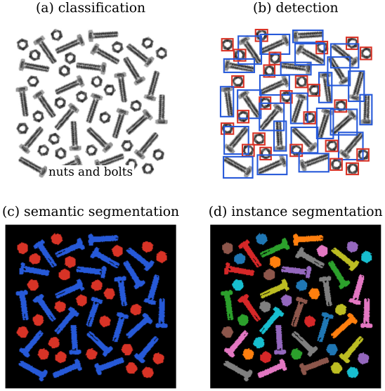
The four answers on one image of 25 nuts and 25 bolts. These outputs come from thresholding, connected components and an eccentricity rule (eccentricity above 0.85 means a bolt), which stand in for a network’s output so that the four tasks can be compared directly.

None of the objects in this image touch, so the instance answer follows from the semantic one by connected components. That shortcut fails in general. In a herd of cows standing shoulder to shoulder, the semantic “cow” mask is one connected blob, and splitting it into animals needs something that reasons about objects. That is why instance segmentation is built on top of a detector.

training is per-pixel classification

Segmentation is supervised learning where the label is itself an image. Every training image comes with a ground-truth mask of the same size. The network outputs \(C\) scores at each pixel, a softmax turns them into probabilities \(p_c(x,y)\), and the loss is the cross-entropy averaged over all \(HW\) pixels: \[ \mathcal{L} = -\frac{1}{HW} \sum_{x=1}^{W} \sum_{y=1}^{H} \log p_{\,y(x,y)}(x,y). \] It is simply \(HW\) ordinary classification losses, averaged. Predicted masks are scored with the Jaccard index (IoU) or the Dice coefficient, per class, and the per-class IoUs are averaged to give the mean IoU (mIoU).

fully convolutional networks

the obvious idea, and its waste

The first idea is to reuse an image classifier one pixel at a time. A single pixel’s colour is useless on its own, since a brown pixel could be cow, soil or a fence post. So the classifier is shown a \(P \times P\) patch centred on the pixel and asked for the class of the centre. The sliding window does exactly this, at every pixel.

It works, but it is enormously wasteful. A \(224 \times 224\) image needs \(50\,176\) forward passes. With \(65 \times 65\) patches, two horizontal neighbours share \(64/65 \approx 98.5\%\) of their pixels, so nearly all the first-layer work for one patch repeats the work already done for its neighbour. Convolutions already share work across overlapping neighbourhoods, so the fix is to convolve the whole image once and read a class off every position of the resulting feature maps.

why a classifier’s architecture will not do

A classification CNN shrinks its maps as it goes deeper. VGG-16 takes a \(224^2\) input through five \(2 \times 2\) poolings to a \(7^2 \times 512\) map, and then its fully connected layers throw the spatial layout away. You could instead keep every layer at full resolution, but the cost is prohibitive. A \(3 \times 3\) layer with \(c_{\text{in}}\) inputs and \(c_{\text{out}}\) outputs on an \(n \times n\) map costs \(9 n^2 c_{\text{in}} c_{\text{out}}\) multiply–accumulates:

map	channels	MACs
\(224^2\)	64 to 64	\(1.85 \times 10^9\)
\(56^2\)	256 to 256	\(1.85 \times 10^9\)
\(224^2\)	256 to 256	\(2.96 \times 10^{10}\)

Halving the resolution twice pays for four times the channels. A network that stays at full resolution must either stay thin, which gives weak features, or become sixteen times as expensive.

downsample, then upsample

The design that works shrinks the map inside the network and grows it back again. High resolution at the ends, low resolution and many channels in the middle, where the expensive layers live.

Definition (Fully convolutional network)

A fully convolutional network (FCN) uses only convolution, pooling and upsampling layers, with no fully connected layer (Long, Shelhamer and Darrell, 2015). For segmentation it is an encoder–decoder. The encoder turns the \(3 \times H \times W\) image into low-resolution, many-channel features. The decoder brings them back to \(C \times H \times W\) class scores. The prediction at each pixel is \[ J(x,y) = \arg\max_c \, \text{score}_c(x,y). \] The whole network is trained end to end on the per-pixel loss.

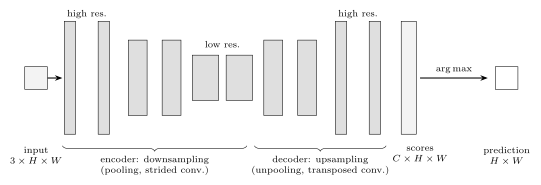
An encoder–decoder FCN. Block height stands for spatial resolution and block width for channel count. The expensive many-channel layers run at low resolution, and the decoder restores the input resolution stage by stage.

Nothing in an FCN depends on the input size, so it accepts any image size (up to the divisibility the poolings need) and labels the whole image in one forward pass. The open question is how the decoder enlarges a map. That is the next section.

upsampling inside the network

The decoder needs layers that undo pooling and strided convolution. There are two families. Fixed rules (unpooling and bilinear interpolation) have no parameters. Learned upsampling (transposed convolution) has a kernel that is trained with everything else.

unpooling

Definition (Unpooling)

Unpooling with factor 2 maps an \(n \times n\) map \(A\) to a \(2n \times 2n\) map by replacing each value with a \(2 \times 2\) block:

nearest neighbour: all four entries equal the value;
fixed position (“bed of nails”): the value goes in the top-left entry and the other three are zero;
max unpooling: each encoder max-pooling layer remembers which entry of each window held the maximum (its switches), and the paired decoder layer puts the value back at that position, with zeros elsewhere.

None of the three has learnable parameters.

Max unpooling is the clever one. Pooling throws away where in each window the strong response was, and max unpooling puts each feature back where it came from, which partly restores the fine position of edges.

Example (Three unpoolings of the same map)

Max-pool the \(4 \times 4\) map below with \(2 \times 2\) windows and stride 2. The maxima are \(5, 6, 7, 8\), found at positions \((1,1), (0,2), (3,0), (3,3)\) (row and column, counted from 0). Suppose the decoder later receives \(\begin{pmatrix}1&2\\3&4\end{pmatrix}\) at this resolution. Then the three rules give: \[ \underbrace{\begin{pmatrix}1&1&2&2\\1&1&2&2\\3&3&4&4\\3&3&4&4\end{pmatrix}}_{\text{nearest}} \quad \underbrace{\begin{pmatrix}1&0&2&0\\0&0&0&0\\3&0&4&0\\0&0&0&0\end{pmatrix}}_{\text{fixed position}} \quad \underbrace{\begin{pmatrix}0&0&2&0\\0&1&0&0\\0&0&0&0\\3&0&0&4\end{pmatrix}}_{\text{max unpooling}} \] The 1 lands at \((1,1)\) because that is where the 5 was, the 2 at \((0,2)\) where the 6 was, and so on.

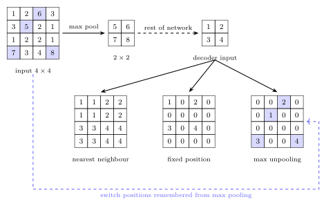
Max pooling records its switch positions (shaded), and max unpooling reuses them.

bilinear upsampling

Nearest-neighbour copies give blocky maps. Bilinear upsampling instead computes each new pixel as a weighted average of its four nearest input pixels, with weights that fall off linearly with distance. In one dimension, upsampling the row \((0, 4)\) to three samples with the end points held fixed gives \((0, 2, 4)\). It has no parameters either, and the result is smooth. The weights are given exactly in the RoI Align section below, where the same interpolation reappears.

Bilinear upsampling is itself a transposed convolution with a fixed “tent” kernel. The original FCN used exactly that observation: it initialised its learned upsampling layers to bilinear interpolation and let training adjust them. A common modern decoder step is bilinear upsampling followed by an ordinary \(3 \times 3\) convolution, which sidesteps the checkerboard problem described below.

transposed convolution

A strided convolution moves its kernel \(s\) pixels in the input for each pixel of output, and each output is a dot product of many inputs. A transposed convolution reverses both roles. The kernel moves \(s\) pixels in the output for each input pixel, and each input value scatters a weighted copy of the kernel into the output. Where copies overlap, they add.

Definition (Transposed convolution)

Let \(A\) be \(n \times n\) and \(h\) a \(k \times k\) kernel. The transposed convolution with stride \(s\) is the map \[ B(u,v) = \sum_{i=0}^{n-1} \sum_{j=0}^{n-1} A(i,j)\, h(u - si,\; v - sj), \] with \(h = 0\) outside its \(k \times k\) support. Each \(A(i,j)\) weights a copy of the kernel whose top-left corner sits at \((si, sj)\). Padding \(p\) crops \(p\) rows and columns from each border of \(B\). The kernel entries are learned, so the layer learns how to upsample. Other names are fractionally strided convolution, up-convolution, and “deconvolution”, which is a misnomer: the layer does not invert a convolution.

Definition (Algorithm: Transposed convolution (one channel))

Input \(A\) (\(n \times n\)), kernel \(h\) (\(k \times k\)), stride \(s\), padding \(p\), output padding \(a \in \{0, \dots, s-1\}\).

Set \(B\) to zeros of side \((n-1)s + k + a\).
For every \((i,j)\), add \(A(i,j) \cdot h\) into the \(k \times k\) block of \(B\) whose top-left corner is \((si, sj)\).
Crop \(p\) rows and columns from the top and left, and \(p\) from the bottom and right.
Return \(B\), whose side is \((n-1)s - 2p + k + a\).

With several channels there is one kernel per (input, output) channel pair and the scattered copies are summed over input channels, so the parameter count is \(k^2 c_{\text{in}} c_{\text{out}}\), the same as an ordinary convolution with the same shape.

Example (Stride 1, by hand)

Take input \(A = \begin{pmatrix}0&1\\2&3\end{pmatrix}\), the same matrix as the kernel \(h\), stride 1 and no padding. The output has side \((2-1) \cdot 1 + 2 = 3\). Each input value scales a copy of the kernel placed at its own offset, and the four copies add: \[ \begin{pmatrix}0&0&0\\0&0&0\\0&0&0\end{pmatrix} + \begin{pmatrix}0&0&1\\0&2&3\\0&0&0\end{pmatrix} + \begin{pmatrix}0&0&0\\0&2&0\\4&6&0\end{pmatrix} + \begin{pmatrix}0&0&0\\0&0&3\\0&6&9\end{pmatrix} = \begin{pmatrix}0&0&1\\0&4&6\\4&12&9\end{pmatrix}. \] The entries \(4 = 2+2\), \(6 = 3+3\) and \(12 = 6+6\) are where copies overlapped. A \(2 \times 2\) map has become \(3 \times 3\).

the output-size trap

Here is the trap. You want to undo a \(3 \times 3\), stride-2, padding-1 convolution, which maps \(4 \times 4\) to \(2 \times 2\). The natural guess is a transposed convolution with the same \(k = 3\), \(s = 2\), \(p = 1\), applied to the \(2 \times 2\) map. It gives \(3 \times 3\), not \(4 \times 4\).

Proposition (Output size of a transposed convolution)

A transposed convolution with kernel \(k\), stride \(s\), padding \(p\) and output padding \(a\) maps side \(n_{\text{in}}\) to \[ n_{\text{out}} = (n_{\text{in}} - 1)\, s - 2p + k + a. \] An ordinary convolution with the same \(k, s, p\) maps \(n_{\text{out}}\) back to \(n_{\text{in}}\), whatever the value of \(a\) in \(\{0, \dots, s-1\}\).

With \(n_{\text{in}} = 2\), \(k = 3\), \(s = 2\), \(p = 1\) and no output padding, the formula gives \((2-1) \cdot 2 - 2 + 3 + 0 = 3\). A convolution with the same settings maps both 3 and 4 to 2, and the transposed convolution has to pick one of them; without being told, it picks the smaller. Setting \(a = 1\) (output_padding=1 in PyTorch) gives 4.

Example (Stride 2, and where the 3 comes from)

Take \(A = \begin{pmatrix}1&2\\3&4\end{pmatrix}\), a \(3 \times 3\) kernel of ones, and stride 2. The copies start at offsets 0 and 2, so the uncropped output is \(5 \times 5\), and neighbouring copies overlap in one row or column: \[ \begin{pmatrix}1&1&3&2&2\\1&1&3&2&2\\4&4&10&6&6\\3&3&7&4&4\\3&3&7&4&4\end{pmatrix}. \] Padding \(p = 1\) crops one row and column from every side and leaves \(\begin{pmatrix}1&3&2\\4&10&6\\3&7&4\end{pmatrix}\), which is \(3 \times 3\). Output padding \(a = 1\) keeps one extra row and column at the bottom and right, which gives the \(4 \times 4\) you wanted.

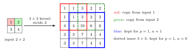
The red and green kernel copies overlap in one column, which is summed. Padding and output padding choose which part of the 5 by 5 result survives: the dotted 3 by 3 for p = 1, a = 0, or the blue 4 by 4 for p = 1, a = 1.

Look at the centre value, 10. It is where four copies overlapped, whereas the corners got one copy each. When the kernel size is not a multiple of the stride, this uneven overlap is built into the layer, and it is a known source of checkerboard artefacts in learned upsampling (Odena, Dumoulin and Olah, 2016). Two common remedies are a kernel size divisible by the stride (U-Net uses \(k = s = 2\), which gives no overlap at all) and resize-then-convolve.

why the formula holds

Proof (Output size of a transposed convolution)

The kernel copies start at offsets \(0, s, \dots, (n_{\text{in}} - 1)s\), and the last one ends at \((n_{\text{in}} - 1)s + k - 1\). So the uncropped output has side \((n_{\text{in}} - 1)s + k\). Padding removes \(2p\) and output padding adds \(a\), which gives the formula.

For the inversion, recall that a convolution maps side \(m\) to \(\lfloor (m + 2p - k)/s \rfloor + 1\). Substituting \(m = (n_{\text{in}} - 1)s - 2p + k + a\) gives \[ \left\lfloor \frac{(n_{\text{in}} - 1)s + a}{s} \right\rfloor + 1 = n_{\text{in}}, \] because \(0 \le a < s\). The floor is the whole story. For \(s > 1\), a strided convolution sends \(s\) different input sizes to the same output size, so its inverse is ambiguous, and \(a\) is the extra bit that chooses among them.

why “transposed”

A convolution is linear, so it is multiplication by a matrix \(\mathbf C\) on the flattened input, \(\mathbf y = \mathbf C \mathbf x\). The transposed convolution with the same kernel, stride and padding is multiplication by \(\mathbf C^\top\). Entry \(C_{mi}\) is the weight with which input \(i\) feeds output \(m\), so \((\mathbf C^\top \mathbf y)_i = \sum_m C_{mi} y_m\) sends every output back to the inputs that fed it, weighted by the same kernel entry. That is exactly the scatter-and-add above. It restores the shape of \(\mathbf x\), not its values, because \(\mathbf C\) is not invertible in general.

Example (The matrix view in one dimension)

Kernel \((1,2,3)\), stride 1, no padding, input length 4, so the output has length 2: \[ \mathbf C = \begin{pmatrix}1&2&3&0\\0&1&2&3\end{pmatrix}, \qquad \mathbf C^\top \begin{pmatrix}1\\-1\end{pmatrix} = \begin{pmatrix}1\\1\\1\\-3\end{pmatrix}. \] Scattering directly gives the same answer: \[ 1 \cdot (1,2,3,0) + (-1) \cdot (0,1,2,3) = (1,1,1,-3). \]

choosing an upsampler

layer	parameters	watch out for
nearest neighbour	none	blocky output
max unpooling	none	needs the paired switches
bilinear	none	smooth, cannot learn
transposed convolution	\(k^2 c_{\text{in}} c_{\text{out}}\)	size ambiguity, checkerboards

Fixed upsamplers are cheap and stable, while transposed convolution lets the network learn what upsampling the task needs. In practice decoders use either a learned \(2 \times 2\), stride-2 transposed convolution (U-Net) or bilinear upsampling followed by a convolution.

U-Net

An encoder–decoder has one structural weakness. The decoder must redraw fine boundaries from the bottleneck, where the precise position of every edge has been pooled away. U-Net keeps everything above (convolutions, downsampling, learned upsampling, end-to-end training) and adds skip connections, which hand the encoder’s high-resolution maps straight across to the decoder.

Definition (U-Net)

U-Net (Ronneberger, Fischer and Brox, 2015) is a fully convolutional encoder–decoder with a skip connection at every resolution.

contracting path: at each of four levels, two unpadded \(3 \times 3\) convolutions with ReLU, then \(2 \times 2\) max pooling. The channel count doubles at each level (64, 128, 256, 512) and reaches 1024 at the bottom.
expanding path: at each level, a \(2 \times 2\) up-convolution (stride-2 transposed convolution) that doubles the size and halves the channels; concatenation with the encoder’s map from the same level, centre-cropped to match (“copy and crop”); then two \(3 \times 3\) convolutions with ReLU.
output: a \(1 \times 1\) convolution from 64 channels to \(C\) class scores per pixel (\(C = 2\) in the original).

The decoder combines what (deep, coarse features) with where (shallow, high-resolution features).

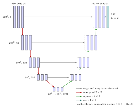
U-Net. Left, the contracting path; right, the expanding path. Grey arrows are the skip connections, which copy and crop an encoder map (dashed) and concatenate it with the upsampled decoder map. Labels give side length and channel count.

U-Net’s skips concatenate channels, whereas ResNet’s residual connections add a block’s input to its output. Both let information bypass layers, but for different reasons: U-Net’s restore spatial detail, while ResNet’s make very deep networks trainable.

every size through U-Net

Example (Sizes from a 572 by 572 tile)

An unpadded \(3 \times 3\) convolution shrinks a side by 2, pooling halves it, and up-convolution doubles it. From a \(572 \times 572\) tile:

encoder: \(572 \to 570 \to 568\), pool \(284 \to 282 \to 280\), pool \(140 \to 138 \to 136\), pool \(68 \to 66 \to 64\), pool \(32\);
bottom: \(32 \to 30 \to 28\), with 1024 channels;
decoder: up to 56, concatenated with the 64 map cropped by 4 per side, \(\to 54 \to 52\); up to 104 (136 cropped by 16), \(\to 102 \to 100\); up to 200 (280 cropped by 40), \(\to 198 \to 196\); up to 392 (568 cropped by 88), \(\to 390 \to 388\);
output: \(388 \times 388 \times 2\).

The output is smaller than the input because every convolution is unpadded. The \(388^2\) prediction covers the centre of the tile, and the border supplies the context those pixels need. Large images are segmented tile by tile with overlapping inputs. The crop is needed because the encoder’s map is always larger than the decoder’s at the same level: at the top, \((568 - 392)/2 = 88\). Modern implementations usually pad the convolutions instead, so that no crop is needed.

what the skips buy

Example (Same network, with and without skips)

Two small networks were trained from scratch on \(64 \times 64\) noisy grey images of discs (class 1) and squares (class 2) on background (class 0), with 800 training images and 100 test images. Everything else was identical: seed 9517, Adam at \(10^{-3}\), 500 steps of 8 images, per-pixel cross-entropy, two encoder levels down to \(16 \times 16\) and two stride-2 transposed convolutions back up. The only difference is that the second network concatenates the encoder’s \(64\) and \(32\) maps into its decoder, as U-Net does.

network	IoU disc	IoU square	mIoU
encoder–decoder	0.707	0.752	0.816
with skips	0.773	0.849	0.873

The skip network has 11% more parameters (116 787 against 105 267) and lifts mIoU from 0.816 to 0.873. Most of the gain is on object boundaries, as the figure shows. Without skips, outlines come out rounded and blotchy, and a disc touching a square partly takes the wrong class, because the decoder has to rebuild every boundary from a \(16 \times 16\) map. With skips, the corners of the squares come out sharp.

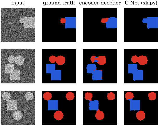
Test images: input, ground truth (red disc, blue square), the plain encoder–decoder, and the same network with U-Net skips.

when to use it, and where it fails

U-Net is the default for semantic segmentation when training images are few and boundaries must be accurate, which is why it dominates biomedical imaging (see the KiTS19 kidney-tumour project). Its failures are the failures of semantic segmentation itself. Touching objects of one class come out as one blob, so counting needs post-processing such as a watershed, or an instance method. Its receptive field is also local, so labels that depend on context across the whole image suffer.

The encoder–decoder-with-skips shape has since been reused with better blocks plugged in:

variant	change	motivation
Attention U-Net	attention gates on the skips	focus on the target organ
ResUNet	residual, dilated blocks	depth, multi-scale context
TransUNet	transformer layers in the encoder	global context

instance segmentation with Mask R-CNN

Semantic segmentation cannot separate touching objects of one class. A detector already separates objects, one box each, but it draws no outline. Mask R-CNN puts the two together: it is Faster R-CNN with an extra branch that predicts a binary mask inside every detected box.

Definition (Mask R-CNN)

Mask R-CNN (He, Gkioxari, Dollár and Girshick, 2017) has two parts.

backbone: a ResNet or ResNeXt of depth 50 or 101 with a feature pyramid network, which extracts features.
head: Faster R-CNN’s region proposal network and per-region class and box outputs, plus a parallel convolutional mask branch that outputs a mask for each region of interest (RoI).

Region features come from RoI Align rather than RoI pooling. Each sampled RoI is trained on the multi-task loss \[ \mathcal L = \mathcal L_{\text{cls}} + \mathcal L_{\text{box}} + \mathcal L_{\text{mask}}. \]

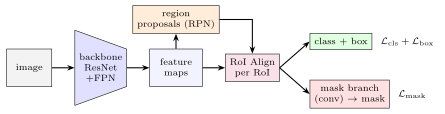
Mask R-CNN: Faster R-CNN’s backbone, proposals and class/box head, with RoI Align and a parallel mask branch.

The mask branch is a small FCN run on each RoI’s features. It outputs one \(28 \times 28\) mask per class, and \(\mathcal L_{\text{mask}}\) is the mean per-pixel binary cross-entropy of the mask for the RoI’s true class only. The other classes’ masks do not enter the loss, so classes never compete at the pixel level. The classification branch decides what the object is, and the mask branch only decides where it is. At test time, the mask of the predicted class is resized to the box and thresholded at 0.5.

why RoI pooling is not good enough

RoI pooling projects each proposal onto the feature map and then rounds twice: once to snap the box to whole feature cells, and again when it splits the snapped window into bins. The pooled features therefore describe a slightly different region from the proposal. For a box this hardly matters, since a box a few pixels off still overlaps the object well. For a pixel-level mask, the same shift moves the boundary.

Example (Snapping error of RoI pooling)

A \(640 \times 480\) image gives a \(20 \times 15\) feature map, a stride of 32. Take a proposal spanning \(x \in [100, 300]\), \(y \in [60, 250]\). Dividing by 32 gives \[ x \in [3.125,\ 9.375], \qquad y \in [1.875,\ 7.8125]. \] Rounding each corner to the nearest cell gives \([3, 9] \times [2, 8]\), which maps back to \([96, 288] \times [64, 256]\) in the image. The four edges have moved by 4, 12, 4 and 6 pixels, and the right edge cuts a 12-pixel strip off the object. The bin split then rounds a second time (6 cells cannot be divided into 7 equal bins), which adds more error.

RoI Align

The fix is to never round. RoI Align keeps the projected box fractional, divides it into exactly equal subregions, and reads the features at a few regular sample points in each subregion by bilinear interpolation.

Definition (Bilinear interpolation)

Let feature values \(f_{i,j}\) sit at integer grid points. At a real point \((x,y)\), write \((i_0, j_0) = (\lfloor x \rfloor, \lfloor y \rfloor)\), \(\alpha = x - i_0\) and \(\beta = y - j_0\). Then \[ f(x,y) = (1-\alpha)(1-\beta) f_{i_0,j_0} + \alpha(1-\beta) f_{i_0+1,j_0} + (1-\alpha)\beta f_{i_0,j_0+1} + \alpha\beta f_{i_0+1,j_0+1}. \] The weights are non-negative and sum to 1, and \(f\) is differentiable in the four features, so gradients flow back to all four neighbours.

Definition (Algorithm: RoI Align)

Feature map \(F\) (\(c \times H_F \times W_F\)) with stride \(\delta\), a proposal \((x_0, y_0, x_1, y_1)\) in image pixels, output size \(P\), and \(r \times r\) samples per subregion.

Divide the box by \(\delta\), with no rounding.
Set the subregion size to \(w = (x_1 - x_0)/P\) and \(h = (y_1 - y_0)/P\), which are fractional.
In subregion \((a,b)\), place the samples at \(x = x_0 + \bigl(a + \tfrac{q + 1/2}{r}\bigr) w\) and \(y = y_0 + \bigl(b + \tfrac{t + 1/2}{r}\bigr) h\), for \(q, t = 0, \dots, r-1\).
Bilinearly interpolate \(F\) at every sample, in every channel.
Max- or average-pool the \(r^2\) samples of each subregion into one value.

The output is \(c \times P \times P\): \(P = 7\) in practice, and \(P = 2\) in the figure below.

Example (RoI Align on the same proposal)

Keep the projected box \([3.125, 9.375] \times [1.875, 7.8125]\) with \(P = 2\) and \(r = 2\). Each subregion is \(3.125\) by \(2.96875\) cells. The top-left subregion samples at a quarter and three quarters of its width and height, which gives \(x \in \{3.906, 5.469\}\) and \(y \in \{2.617, 4.102\}\). Nothing is rounded.

To see one interpolation by hand, suppose \(f_{3,2} = 1\), \(f_{4,2} = 3\), \(f_{3,3} = 2\) and \(f_{4,3} = 6\), and sample at \((3.25, 2.5)\). Then \(\alpha = 0.25\) and \(\beta = 0.5\), so \[ f = 0.375 \cdot 1 + 0.125 \cdot 3 + 0.375 \cdot 2 + 0.125 \cdot 6 = 2.25. \]

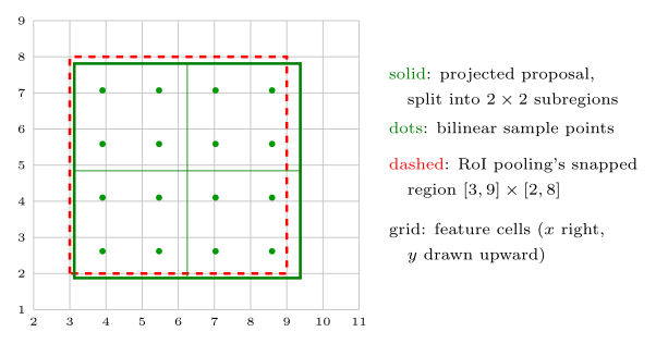
The proposal on the 20 by 15 feature grid (part shown). RoI pooling snaps it to whole cells (red, dashed); RoI Align keeps the fractional box (green), splits it exactly and samples by bilinear interpolation (dots).

when to use it, and where it fails

Use Mask R-CNN when objects must be both told apart and outlined, such as counting touching cells or measuring each animal in a herd. Its failures come from its detector. Every mask lives inside a box, so a missed or misplaced box loses the mask, and non-maximum suppression can delete one of two heavily overlapping instances. Each mask is also predicted at \(28 \times 28\) and stretched to the box, so large objects get coarse boundaries. For amorphous regions with no instances (road, sky, tissue type), an FCN or U-Net is simpler and cheaper.

which tool when

need	use
per-pixel classes, few images	U-Net
per-pixel classes, global context	TransUNet or similar
separate objects of one class	Mask R-CNN
boxes are enough	a detector, see Object Detection

The distinctions people most often get wrong:

unpooling vs transposed convolution: unpooling has no parameters; a transposed convolution learns its kernel, and max unpooling needs its paired pooling layer’s switches.
transposed convolution vs deconvolution: a transposed convolution restores the shape, not the values. It is \(\mathbf C^\top\), not \(\mathbf C^{-1}\).
U-Net skips vs ResNet skips: U-Net concatenates, to restore spatial detail; ResNet adds, to make deep networks trainable.
RoI pooling vs RoI Align: RoI pooling rounds to whole cells, which is fine for boxes; RoI Align never rounds, which masks need.
Mask R-CNN vs Faster R-CNN: the same detector, plus a mask branch, \(\mathcal L_{\text{mask}}\), and RoI Align.

The original papers are short and readable: FCN (Long et al.), U-Net (Ronneberger et al.) and Mask R-CNN (He et al.).

Semantic and Instance Segmentation