Object Detection
A classifier answers “what is in this image?”. A detector answers two questions at once: what objects are present, and where each one is, as a box drawn tightly around it. The output is no longer one label but a list of (class, box) pairs whose length is not known in advance. 𐃏
The modern answer was built in a clear sequence, and each step removes the bottleneck of the one before it. Classify thousands of crops; then classify only a couple of thousand proposed crops (R-CNN); then share one convolutional pass among all of them (Fast R-CNN); then let the network propose the crops itself (Faster R-CNN); then drop the proposal stage altogether (YOLO, SSD) and fix the accuracy that cost (focal loss, RetinaNet). Two small tools run through the whole story: IoU to measure a box, and non-maximum suppression to remove duplicate boxes.
The convolutional building blocks are on the From Convolution to CNNs page (and in CNN from scratch). Turning boxes into pixel masks, with Mask R-CNN and RoI Align, is the job of Semantic and Instance Segmentation.
measuring a box: IoU
A predicted box is never exactly right, so we need one number that says how good it is. Write a box in corner form \(\mathbf b = (x_1, y_1, x_2, y_2)\), top-left and bottom-right.
For two boxes \(\mathbf b\) and \(\mathbf b^*\), with \(|\cdot|\) denoting area, \[ \operatorname{IoU}(\mathbf b, \mathbf b^*) = \frac{|\mathbf b \cap \mathbf b^*|}{|\mathbf b \cup \mathbf b^*|} = \frac{|\mathbf b \cap \mathbf b^*|}{|\mathbf b| + |\mathbf b^*| - |\mathbf b \cap \mathbf b^*|} . \] It is 1 for a perfect box and 0 for disjoint boxes. For axis-aligned boxes the intersection is again a box, \[ [\max(x_1, x_1^*), \min(x_2, x_2^*)] \times [\max(y_1, y_1^*), \min(y_2, y_2^*)] , \] empty when either interval is empty. Benchmarks count a prediction of the right class as correct when \(\operatorname{IoU} \ge 0.5\).
IoU is the Jaccard index applied to two regions, so it punishes errors in position and in size together. That makes it stricter than it looks.
Take \(\mathbf b = (2,2,8,6)\) and \(\mathbf b^* = (4,3,10,8)\).
- Areas: \(|\mathbf b| = 6 \times 4 = 24\) and \(|\mathbf b^*| = 6 \times 5 = 30\).
- Intersection: \([4,8] \times [3,6]\), area \(4 \times 3 = 12\).
- Union: \(24 + 30 - 12 = 42\), so \(\operatorname{IoU} = 12/42 = 2/7 \approx 0.29\).
The boxes overlap visibly, yet the prediction is scored wrong at the 0.5 threshold.
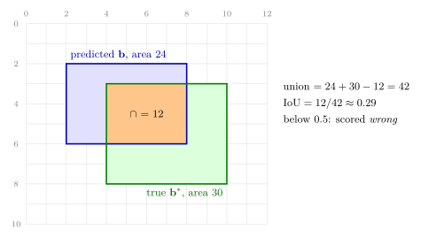
The worked example: two boxes that clearly overlap still have an IoU of only 0.29.
one object: a class head and a box head
If the image is known to hold exactly one object, detection is classification (“what”) plus localisation (“where”). Take any classification CNN, keep its feature vector, and attach two heads in parallel: a fully connected layer to class scores, and a second fully connected layer to four box numbers \((x, y, w, h)\). Train with cross-entropy on the class head plus a squared-error loss on the box head, summed into one loss. A network trained on two objectives through one summed loss is a multi-task network, and every detector below is one.
The squared error is only a proxy for what we want, a large IoU: it is easy to differentiate, but two boxes with equal squared error can have quite different IoU.
Each \(64 \times 64\) scene holds one Chinese-MNIST character (15 classes) of random size (16 to 36 pixels) at a random position on a noisy background, so the true box is known exactly. The network is four convolution-and-pooling blocks (8, 16, 32, 32 channels), a 128-unit fully connected layer, a 15-way class head and a 4-number box head (centre and size as fractions of the image side). The loss is cross-entropy plus 10 times the mean squared box error.
After 30 epochs on 6000 scenes (about 2.3 minutes on four CPU threads), on 1000 fresh scenes:
| measure | value |
|---|---|
| class accuracy | 83.7% |
| mean IoU (median) | 0.62 (0.64) |
| \(\operatorname{IoU} \ge 0.5\) | 81.2% |
| right class and IoU \(\ge 0.5\) | 69.0% |
The training loss fell from 2.89 to 0.15 and had levelled off. The box head never sees a crop: it reads the object’s position straight off the shared feature map.
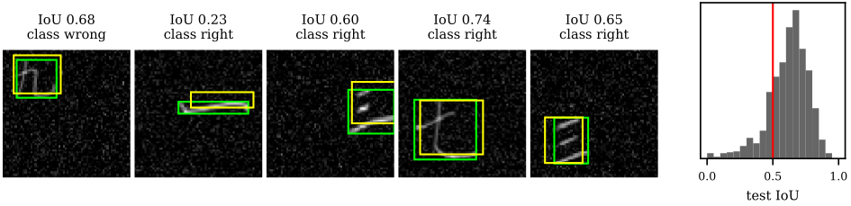
Five test scenes with the true box (green) and the predicted box (yellow), and the histogram of test IoU; the red line is the 0.5 threshold. The second scene has the right class but a box too short and shifted, IoU 0.23.
The two-head network outputs exactly four numbers. An image with two objects needs eight, a herd of zebras needs “many”, and a fixed-size output layer cannot provide a variable number. Everything that follows is a way round this.
many objects: from sliding windows to proposals
The first fix turns detection back into classification. Cut many crops out of the image (a sliding window at several sizes and aspect ratios), run the CNN on each, and let it answer one of the object classes or background. Every crop not called background is a detection.
The trouble is cost. Objects can sit at any position, at any size and with any aspect ratio, so the number of crops is enormous, and each one is a full CNN forward pass. Every method on this page reduces either the number of crops or the cost of each.
selective search
A region proposal method looks at the image once and returns a short list of regions likely to contain some object, whatever its class. Selective search, the proposal method of the first CNN detectors, returns about 2000 boxes per image in a few seconds on a CPU.
Its idea is bottom-up: start from an over-segmentation into many small regions of similar colour (Felzenszwalb and Huttenlocher’s graph-based segmentation), assume objects are unions of these pieces, and build the unions greedily.
Input: an image and a similarity \(S(r_i, r_j)\) between regions. Output: a list \(\mathcal R\) of proposal boxes.
- Over-segment the image into regions \(r_1, \dots, r_n\); put their bounding boxes in \(\mathcal R\).
- Compute \(S(r_i, r_j)\) for every pair of adjacent regions.
- While more than one region remains: merge the most similar adjacent pair into \(r_t = r_i \cup r_j\), add the bounding box of \(r_t\) to \(\mathcal R\), and recompute similarities only between \(r_t\) and its neighbours.
- Return \(\mathcal R\): one box per node of the merge tree, \(2n - 1\) in all.
Three design choices explain the details. Every level of the merge hierarchy contributes boxes, so all object scales are covered. The similarity combines colour, texture, size and fill terms, and the whole procedure is rerun in several colour spaces, because no single cue groups every object (a cat is one texture but many colours, a car one colour but many textures). And a merged region’s histograms and size come from its parts without revisiting pixels, which keeps it fast.
A simplified version on the portrait at half resolution: 148 initial regions; similarity is colour-histogram intersection plus size similarity \(1 - (|r_i| + |r_j|)/|I|\) (which merges small regions first) plus fill (which prefers pairs that fill their joint bounding box). Merging down to one region gives \(2 \times 148 - 1 = 295\) proposals. Among the largest are boxes round the face, the cap, the whole head and the torso, found by merging rather than by any window scan.
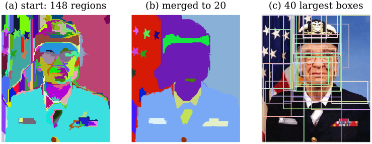
Simplified selective search: (a) the over-segmentation into 148 regions; (b) the hierarchy after greedy merging to 20 regions; (c) the 40 largest of the 295 proposals, excluding the whole image.
When it fails. Selective search is a fixed, hand-designed grouping. An object whose parts differ from each other but resemble the background (a camouflaged animal, a patterned shirt against a busy wall) may never be formed as one region, and no later stage can recover a missed proposal. It also costs seconds per image, which becomes the bottleneck once the network is fast.
When to use it. When proposals are needed without any training, in a new domain with no box labels. Inside a trained detector, the learned region proposal network below replaces it.
the R-CNN line
Three detectors, each fixing the previous one’s slowest step. The figure shows them side by side.
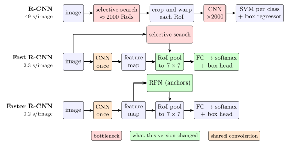
R-CNN runs the CNN once per proposal; Fast R-CNN runs it once per image and pools each proposal out of the feature map; Faster R-CNN also learns the proposals from that feature map. Test times per image with VGG-16.
R-CNN
R-CNN (“regions with CNN features”) is crop-and-classify made affordable by proposals.
- Extract about 2000 regions of interest (RoIs) with selective search.
- For each RoI: crop it, warp (resize) it to the CNN’s fixed input size, and compute a CNN feature vector.
- Score the vector with one linear SVM per class, and refine the box with that class’s box regressor.
- Remove duplicate boxes with non-maximum suppression.
It works, and it is very slow. Training is three separate stages (fine-tune the CNN on proposals, fit the SVMs, fit the box regressors) that cannot correct each other; the features of every proposal of every training image are written to disk (2.5 GPU-days and hundreds of gigabytes for the 5000 PASCAL VOC 2007 images); and at test time each image needs about 2000 independent forward passes, 47 seconds on a GPU.
why a CNN needs a fixed input size
The 2000 passes are mostly redundant, since overlapping proposals send the same pixels through the same convolutions again and again. The obvious fix is to run the convolutions once on the whole image and cut each proposal out of the feature map. What stops us is the warp: why does the network need a fixed input at all?
The convolutional layers do not care. A convolution slides the same small kernel over any height and width and simply produces a proportionally sized output. The fully connected layers do care: they multiply a vector of fixed length by a weight matrix of fixed shape, so if the feature map changes size the flattened vector changes length and the product is undefined. What is needed is a layer that turns a window of any size into a tensor of fixed size. Spatial pyramid pooling (SPP-Net) did it with several grid levels; Fast R-CNN uses the single-level version.
Fast R-CNN and RoI pooling
Let the backbone have total stride \(s\) and output a feature map of size \(C \times H \times W\), and let a proposal have corners \((x_1, y_1, x_2, y_2)\) in pixels. RoI pooling to \(H_o \times W_o\):
- project the proposal onto the feature map, \((x_1/s, y_1/s, x_2/s, y_2/s)\);
- snap the projected box to whole feature-map cells;
- divide the snapped window into an \(H_o \times W_o\) grid of roughly equal cells;
- max-pool inside each cell, separately in each channel.
The output is \(C \times H_o \times W_o\) for every proposal, whatever its size. Fast R-CNN uses \(H_o = W_o = 7\).
A snapped window of 5 rows and 4 columns must become \(2 \times 2\). Split the rows \(2 + 3\) and the columns \(2 + 2\), then take the maximum of each block. In one channel: \[ \left(\begin{array}{cc|cc} 0&1&8&1\\ 6&2&7&2\\ \hline 7&9&9&1\\ 4&4&1&7\\ 5&8&3&3 \end{array}\right) \;\xrightarrow{\ \max\text{ per block}\ }\; \begin{pmatrix} 6&8\\ 9&9 \end{pmatrix} . \] The same happens in every channel. Region features always have the same size even when the regions do not.
The snap in step 2 shifts the box by a fraction of a cell, which is several pixels at stride 16: projecting \((100, 50, 200, 150)\) from a \(224 \times 224\) image onto a \(14 \times 14\) map gives \((6.25, 3.125, 12.5, 9.375)\), and rounding moves the edges by up to 10 pixels. That is harmless for classification but hurts pixel-accurate masks, which is why Mask R-CNN replaces RoI pooling with RoI Align (see Semantic and Instance Segmentation).
- Pass the entire image through the convolutional backbone once, giving a feature map.
- For each selective-search proposal: RoI-pool its window to \(C \times 7 \times 7\) and pass it through fully connected layers.
- Two sibling heads: a softmax over the \(C_{\text{obj}} + 1\) classes (the objects plus background), and a linear layer giving a box correction for each object class.
Both heads are trained together with one multi-task loss: log loss on the class plus a robust box loss, the box term switched off for background regions, \[ \mathcal L = -\log p_{c^*} + \lambda\, [c^* \ne \text{background}] \sum_{j \in \{x,y,w,h\}} \operatorname{smooth}_{L_1}(t_j - t_j^*) . \] Smooth \(L_1\) is \(\tfrac12 z^2\) for \(|z| < 1\) and \(|z| - \tfrac12\) otherwise: quadratic near zero, so gradients shrink as the box converges, and linear for large errors, so one badly wrong proposal cannot dominate a batch (\(\operatorname{smooth}_{L_1}(3) = 2.5\) against \(\tfrac12 \cdot 3^2 = 4.5\)).
Training is now end to end and nothing is cached to disk. The timings, after Girshick (2015) and Ren et al. (2015):
| method | train (h) | test (s/image) | without proposals |
|---|---|---|---|
| R-CNN | 84 | 49 | 47 |
| SPP-Net | 25.5 | 4.3 | 2.3 |
| Fast R-CNN | 8.75 | 2.3 | 0.32 |
| Faster R-CNN | – | 0.2 | – |
Read the Fast R-CNN row: of its 2.3 seconds, about 2 (86%) are selective search. The network is no longer the bottleneck; the proposals are.
Faster R-CNN: learning the proposals
The feature maps that Fast R-CNN uses to classify regions already encode where objects are, so they can also generate the regions. Faster R-CNN puts a small network on the shared feature map to do that.
Anchors are a fixed set of \(n_a\) reference boxes of preset sizes and aspect ratios, centred at every feature-map position. Faster R-CNN uses \(n_a = 9\): areas \(128^2, 256^2, 512^2\) times ratios \(1{:}1, 1{:}2, 2{:}1\). The detector never predicts a box from nothing: it classifies each anchor and predicts a correction from the anchor to the object.
A region proposal network (RPN) slides a \(3 \times 3\) window over the backbone’s feature map, maps each window to an intermediate feature, and feeds it to two sibling \(1 \times 1\) convolutions: a cls layer with \(2n_a\) outputs (object or not, per anchor) and a reg layer with \(4n_a\) outputs (a box correction per anchor). Anchors with high object scores, moved by their corrections, are the proposals. Being convolutional, the same weights serve every position.
A 512-channel feature map of \(11 \times 15\) positions with 9 anchors each gives \(165 \times 9 = 1485\) anchors. The RPN outputs \(18 + 36 = 54\) numbers per position, \(165 \times 54 = 8910\) per image. The 1485 anchors overlap heavily, so most surviving proposals are near-duplicates: non-maximum suppression thins them out.
The correction is parameterised relative to the anchor’s centre \((x_a, y_a)\) and size \((w_a, h_a)\): \[ t_x = \frac{x - x_a}{w_a}, \quad t_y = \frac{y - y_a}{h_a}, \quad t_w = \log\frac{w}{w_a}, \quad t_h = \log\frac{h}{h_a} . \] Dividing by the anchor size makes the target scale-free, and the logarithm makes doubling and halving equally large corrections. An anchor centred at \((100, 100)\) of size \(128 \times 128\) and a true box centred at \((110, 90)\) of size \(160 \times 120\) give targets \(t^* \approx (0.078, -0.078, 0.223, -0.065)\).
Faster R-CNN is then the RPN plus Fast R-CNN on one shared backbone, trained jointly with four losses: RPN object-or-not, RPN anchor-to-proposal correction, final classification, and final proposal-to-object correction. It detects in about 0.2 s per image, 245 times faster than R-CNN.
the RPN loss and sampling
For a mini-batch of anchors \(i\) with predicted object probability \(p_i\), label \(p_i^* \in \{0, 1\}\), predicted correction \(t_i\) and target \(t_i^*\), \[ \mathcal L = \frac{1}{N_{\text{cls}}} \sum_i L_{\text{cls}}(p_i, p_i^*) + \lambda \frac{1}{N_{\text{reg}}} \sum_i p_i^* L_{\text{reg}}(t_i, t_i^*) , \] with \(L_{\text{cls}}\) the log loss, \(L_{\text{reg}}\) smooth \(L_1\), \(N_{\text{cls}} \approx 256\) (the mini-batch) and \(N_{\text{reg}} \approx 2400\) (the anchor locations). The factor \(p_i^*\) switches regression off for negative anchors. With \(\lambda = 10\) the two terms weigh about the same.
Per anchor, the classification term carries weight \(1/256 \approx 0.0039\) and the regression term \(\lambda/N_{\text{reg}} = 10/2400 \approx 0.0042\). They agree to within 7%, so neither task dominates.
Almost every anchor lies on background; trained on all of them the network would mostly learn what background looks like. The R-CNN family therefore samples: the RPN’s mini-batch is 256 anchors, 128 positive and 128 negative, padded with negatives when an image has fewer positives (40 positives give 216 negatives); the detector stage keeps negatives to at most three per positive, or uses online hard example mining, which samples the anchors with the highest current loss.
non-maximum suppression
Every detector above fires several times on one object: neighbouring anchors or proposals all overlap it and all score highly. Non-maximum suppression (NMS) keeps the best box of each overlapping group. (It shares a name, and nothing else, with the edge-thinning step in Canny.)
Input: scored boxes and an IoU threshold \(\tau\) (for example 0.7). Output: the kept set \(\mathcal K\).
- Start with \(\mathcal K\) empty and \(\mathcal B\) all boxes.
- Move the highest-scoring box \(m\) from \(\mathcal B\) to \(\mathcal K\).
- Delete from \(\mathcal B\) every box with \(\operatorname{IoU}(\cdot, m) > \tau\).
- Repeat from step 2 until \(\mathcal B\) is empty.
At most \(n\) rounds of at most \(n\) IoUs, so \(O(n^2)\). In a detector NMS runs separately for each class.
Five boxes with scores: \(A = (10,10,50,50)\), 0.95; \(B = (12,12,52,52)\), 0.90; \(C = (20,20,60,60)\), 0.80; \(D = (60,10,100,50)\), 0.75; \(E = (62,14,100,52)\), 0.60. The non-zero IoUs are \[ \operatorname{IoU}(A,B) = 0.82, \quad \operatorname{IoU}(A,C) = 0.39, \quad \operatorname{IoU}(B,C) = 0.47, \quad \operatorname{IoU}(D,E) = 0.82 . \] With \(\tau = 0.7\):
- keep \(A\); delete \(B\) (0.82); \(C\) survives (0.39);
- keep \(C\), the best remaining; it overlaps neither \(D\) nor \(E\);
- keep \(D\); delete \(E\) (0.82).
The result is \(\{A, C, D\}\). With \(\tau = 0.3\) the box \(C\) goes too, since \(\operatorname{IoU}(A,C) = 0.39 > 0.3\), leaving \(\{A, D\}\). Whether \(C\) is a second object or a sloppy duplicate of \(A\) is exactly what \(\tau\) decides.
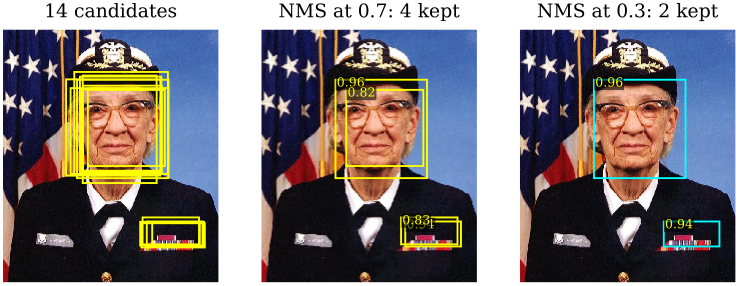
Fourteen scored candidates jittered round the face and the ribbon bar. At threshold 0.7 four boxes survive, two per object, because the jittered duplicates overlap the winner by less than 0.7; at 0.3 one box per object survives (scores 0.96 and 0.94).
When it fails. The threshold trades two errors. A high \(\tau\) removes only near-duplicates and can leave two boxes on one object; a low \(\tau\) removes more duplicates but can delete a genuine second object that overlaps the first: two people walking side by side, or anyone in a crowd. No single threshold is right for both a sparse street and a packed stadium.
one-stage detectors: SSD and YOLO
Every R-CNN-style detector has two stages: propose regions, then classify and refine each one. A one-stage detector replaces both with a single network that maps the image straight to boxes and classes at every position.
| family | members | classifies | strength |
|---|---|---|---|
| two-stage | R-CNN, Fast, Faster R-CNN | a few thousand proposals | accuracy |
| one-stage | SSD, YOLO, RetinaNet | tens of thousands of boxes | speed |
SSD
The single shot multibox detector removes proposals and resampling with three changes: small convolutional filters, not fully connected layers, predict class scores and box offsets at every position; each default box shape has its own predictor; and predictors sit on several feature maps of decreasing resolution, each covering one range of object sizes.
A pre-trained backbone (VGG-16 or ResNet) plus extra convolutional layers. At each position of each of several feature maps, a \(3 \times 3\) convolution outputs, for each of \(n_a\) default boxes, \(C_{\text{obj}} + 1\) class scores and 4 box offsets: \(n_a(C_{\text{obj}} + 5)\) channels. All predictions are pooled and filtered by NMS.
On a \(300 \times 300\) input SSD predicts from six maps: \[ 38^2 \cdot 4 + 19^2 \cdot 6 + 10^2 \cdot 6 + 5^2 \cdot 6 + 3^2 \cdot 4 + 1^2 \cdot 4 = 5776 + 2166 + 600 + 150 + 36 + 4 = 8732 \] boxes per class. With PASCAL VOC’s 21 classes a layer with \(n_a = 4\) needs \(4 \times (21 + 4) = 100\) output channels. Compare Faster R-CNN’s 1485 anchors: one-stage detectors classify far more candidates.
The large maps (\(38 \times 38\), small receptive fields) catch small objects and the small maps catch large ones. Data augmentation turned out to be crucial, and more default box shapes and more output layers both helped.
YOLO
“You only look once” treats detection as one regression problem, from pixels straight to box coordinates and class probabilities, solved by one network applied once to the whole image.
Divide the image into an \(S \times S\) grid. The cell containing an object’s centre is responsible for it. Each cell predicts \(n_b\) boxes, each as 4 coordinates plus an objectness confidence, and one set of \(C\) class probabilities, so the output is an \(S \times S \times (5n_b + C)\) tensor. At test time each box’s confidence times the cell’s class probabilities gives class-specific scores, and NMS removes duplicates.
On PASCAL VOC, \(S = 7\), \(n_b = 2\), \(C = 20\). Per cell: \(2 \times 5 = 10\) box numbers plus 20 class probabilities, 30 in all. The output is \(7 \times 7 \times 30 = 1470\) numbers describing \(98\) boxes. “Image, CNN, \(7 \times 7 \times 30\)” is the entire detector.
Looking once makes it fast. The published comparison on PASCAL VOC 2007 (Redmon et al., 2016):
| detector | mAP (%) | frames/s |
|---|---|---|
| Fast YOLO | 52.7 | 155 |
| YOLO | 63.4 | 45 |
| Fast R-CNN | 70.0 | 0.5 |
| Faster R-CNN, VGG-16 | 73.2 | 7 |
The error analysis against Fast R-CNN is the interesting part. YOLO makes far more localisation errors (right class, IoU between 0.1 and 0.5: 19.0% of its top detections against 8.6%), because each coarse cell predicts only two boxes. It makes far fewer background errors (firing on nothing: 4.75% against 13.6%), because it sees the whole image and so the context of every box. YOLO has since become a large family, from YOLOv2 and v3 through v4 to v11 and variants such as YOLOX and YOLO-World.
why one-stage detectors trailed in accuracy
Both families face an extreme imbalance between object and background candidates, but handle it differently. In a two-stage detector the proposal stage cuts the candidates to about 2000, discarding most background, and the second stage then fixes the foreground-to-background ratio at \(1{:}3\) or mines hard examples. A one-stage detector must score about 100,000 candidates densely covering positions, scales and shapes, and almost all are easy background. Each easy negative has a tiny loss, but there are so many that their sum swamps the training signal from the few objects.
focal loss, feature pyramids and RetinaNet
The cure has two parts: a loss that ignores easy examples, and features that are semantically strong at every resolution.
focal loss
For a binary label with predicted positive-class probability \(p\), let \(p_t = p\) for a positive example and \(p_t = 1 - p\) for a negative one, so cross-entropy is \(-\log p_t\). The focal loss with focusing parameter \(\gamma \ge 0\) is \[ \operatorname{FL}(p_t) = -(1 - p_t)^{\gamma} \log p_t . \] \(\gamma = 0\) is cross-entropy. Lin et al. (2017) use \(\gamma = 2\), with a class weight \(\alpha = 0.25\) on positives.
The factor \((1 - p_t)^\gamma\) is near 0 for well-classified examples and near 1 for badly classified ones, so it silences the easy examples and leaves the hard ones almost untouched.
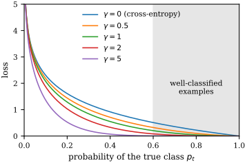
Focal loss against the probability of the true class for several \(\gamma\). Larger \(\gamma\) flattens the loss over the well-classified region (shaded), where the easy negatives live.
Take 100,000 easy negatives with \(p_t = 0.99\) and 100 hard positives with \(p_t = 0.3\).
- Cross-entropy: the negatives contribute \(100\,000 \times 0.01005 = 1005\) and the positives \(100 \times 1.204 = 120.4\). The easy negatives carry 8.3 times the loss of the objects.
- Focal loss with \(\gamma = 2\): each negative is multiplied by \((0.01)^2 = 10^{-4}\), total 0.10; each positive by \((0.7)^2 = 0.49\), total 59.0. The objects now carry almost all of it.
For a single example, at \(p_t = 0.9\) the loss drops by a factor of 100; at \(p_t = 0.1\) only by a factor of 1.23.
feature pyramid networks
Deeper in a CNN, feature maps lose resolution and gain meaning: early maps are sharp but know little about objects, late maps know what is there but only coarsely where. SSD predicts from several resolutions, but its high-resolution maps are semantically weak, which is why it struggles with small objects.
Take the backbone’s bottom-up maps \(C_2, C_3, \dots\), each half the resolution of the last, and build a top-down pathway of maps \(P_l\) at the same resolutions, starting from the coarsest: \[ P_l = \operatorname{Conv}_{1 \times 1}(C_l) + \operatorname{Upsample}_{2\times}(P_{l+1}) . \] The \(1 \times 1\) lateral convolution matches channel counts; the upsampling brings the coarser, semantically stronger map to the same size before the element-wise sum. A prediction head runs at every level, and every level now has strong semantics.
RetinaNet
RetinaNet is a one-stage detector built from both remedies: a ResNet backbone with an FPN, plus focal loss. At every pyramid level two small fully convolutional subnetworks (four \(3 \times 3\) convolutions of 256 channels each, shared across levels) predict, for every position and anchor, the class probabilities and the box offset. The result on COCO (Lin et al., 2017; AP is COCO’s metric, below):
| detector | AP | ms/image |
|---|---|---|
| YOLOv2 | 21.6 | 25 |
| SSD513 | 31.2 | 125 |
| FPN Faster R-CNN | 36.2 | 172 |
| RetinaNet-50-500 | 32.5 | 73 |
| RetinaNet-101-800 | 37.8 | 198 |
The largest RetinaNet beats the best two-stage detector listed, and the RetinaNet curve lies above every other detector at every speed in the paper. With the imbalance handled, one stage is as accurate as two.
how detectors are scored: AP and mAP
A detector outputs ranked, scored boxes, so it is scored by how its precision and recall trade off as the confidence threshold falls. A predicted box is a true positive if its IoU with an unmatched ground-truth box of the same class reaches the threshold (commonly 0.5); otherwise it is a false positive, and every ground-truth box left unmatched is a false negative.
For one class, sort the \(K\) detections by decreasing confidence and let \(P_k\), \(R_k\) be the precision and recall of the top \(k\), with \(R_k\) the number of true positives in the top \(k\) divided by the number of ground-truth objects. The average precision is the area under the precision-recall curve, \[ \text{AP} = \sum_{k=1}^{K} P_k \,(R_k - R_{k-1}), \qquad R_0 = 0 , \] a sum over the ranks where recall rises. Interpolated AP replaces \(P_k\) by \(\max_{k’ : R_{k’} \ge R_k} P_{k’}\), removing the zig-zags. The mean average precision is the mean over the \(C\) classes, \(\text{mAP} = \frac1C \sum_j \text{AP}_j\).
There are 5 pedestrians. Sorted by confidence and matched at IoU 0.5, the detector’s 8 boxes are TP, FP, TP, TP, FP, TP, FP, FP.
| rank | result | \(P_k\) | \(R_k\) |
|---|---|---|---|
| 1 | TP | 1/1 | 0.2 |
| 2 | FP | 1/2 | 0.2 |
| 3 | TP | 2/3 | 0.4 |
| 4 | TP | 3/4 | 0.6 |
| 5 | FP | 3/5 | 0.6 |
| 6 | TP | 4/6 | 0.8 |
| 7 | FP | 4/7 | 0.8 |
| 8 | FP | 4/8 | 0.8 |
- Recall rises by 0.2 at ranks 1, 3, 4 and 6, so \(\text{AP} = 0.2\,(1 + 0.667 + 0.75 + 0.667)\), which is \(0.617\).
- Interpolated precisions at those recalls are 1, 0.75, 0.75, 0.667, so interpolated AP is \(0.633\).
- One pedestrian is never found, so recall stops at 0.8 and AP can never exceed 0.8.
- With a second class at AP 0.45, \(\text{mAP} = (0.617 + 0.45)/2 = 0.53\).
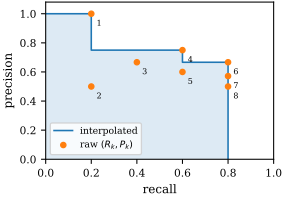
The eight ranked detections as (recall, precision) points, numbered by rank, and the interpolated curve; the shaded area is the interpolated AP, 0.633.
AP rewards a detector that finds every object (high final recall) and ranks its correct boxes above its mistakes (high precision early). Benchmarks differ in the matching threshold: PASCAL VOC uses IoU 0.5, while COCO’s headline “AP” averages over thresholds \(0.50, 0.55, \dots, 0.95\) and also reports AP\(_{50}\), AP\(_{75}\) and AP for small, medium and large objects. A COCO AP of 37.8 and a VOC mAP of 73.2 are therefore not comparable numbers.
which detector, and where each fails
| need | use | watch out for |
|---|---|---|
| accuracy on still images | Faster R-CNN with FPN | about 0.2 s/image: not real time |
| real-time video | YOLO | small objects sharing a cell |
| speed with accuracy | RetinaNet | elongated shapes, crowds |
| proposals without labels | selective search | camouflage; seconds per image |
- Faster R-CNN (with an FPN backbone) when accuracy matters more than speed: small or overlapping objects in still images.
- YOLO for real-time video, but each coarse cell predicts only a couple of boxes and one set of class probabilities, so it localises loosely and under-detects several small objects whose centres share a cell (a flock of birds).
- SSD fails on small objects because its high-resolution maps are semantically weak; an FPN is the fix.
- RetinaNet gives one-stage speed with two-stage accuracy. Like every anchor-based detector it regresses poorly for shapes no anchor resembles (very elongated objects), and like every detector that ends in NMS it can delete a true object overlapping another by more than \(\tau\).
Since 2018 the field has moved on to anchor-free and end-to-end detectors (CornerNet, CenterNet, DETR), which predict object centres or corners, or a set of boxes directly, and some of which need no NMS at all. Open implementations of everything on this page are in Detectron2 and MMDetection.
further reading
- Szeliski, Computer Vision: Algorithms and Applications, 2nd ed., §6.3.3 (object detection).
- Girshick et al., Rich feature hierarchies for accurate object detection (R-CNN, 2014).
- Girshick, Fast R-CNN (2015).
- Ren et al., Faster R-CNN (2015).
- Redmon et al., You Only Look Once (2016).
- Liu et al., SSD: Single Shot MultiBox Detector (2016).
- Lin et al., Feature Pyramid Networks for Object Detection (2017).
- Lin et al., Focal Loss for Dense Object Detection (RetinaNet, 2017).
see also
- From Convolution to CNNs – the backbones every detector runs on
- Semantic and Instance Segmentation – Mask R-CNN and RoI Align, from boxes to masks
- Classical Segmentation – the over-segmentation behind selective search
Backlinks (4)
1. Classical Segmentation /wiki/computer-vision/segmentation/
2. From Convolution to CNNs /wiki/computer-vision/cnns/
3. Semantic and Instance Segmentation /wiki/computer-vision/dense-prediction/
4. Computer Vision /wiki/computer-vision/
I think taking a course in a subject that you are interested in is never particularly a bad thing.
Comments