Seeing in Frequency

Spatial filtering slides a small kernel over the pixels. This page looks at the same image through a different lens: as a sum of waves. In that view blurring keeps the slow waves and throws away the fast ones, a periodic artefact is a handful of bright dots that can be deleted one by one, and an edge detector is a filter that keeps a ring of middle frequencies. The Fourier transform is the change of lens; the convolution theorem is what makes it worth the trouble, because it turns convolution into multiplication. 𐃏

Convolution in neural networks is on the CNN from scratch page; the scale-space machinery that this page’s difference of Gaussians feeds into is on the SIFT, Matching and Stitching page.

aliasing: why frequency is the right language

Halve the rows and columns of a photograph and enlarge it back: the large shapes survive, the leaf texture does not, and no enlarging brings it back. A coarser grid cannot hold fast intensity changes, so something must happen to them. Either they are removed first, or they come back disguised as slower patterns that were never in the scene.

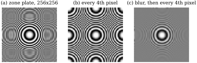
A zone plate \(0.5+0.5\cos(\pi r^2/512)\), whose local frequency \(r/512\) cycles per pixel grows with distance \(r\) from the centre. (b) Keeping every fourth pixel: rings finer than \(1/8\) cycle per pixel (beyond \(r=64\)) cannot be represented and fold back as false coarse rings. (c) A Gaussian blur (\(\sigma=2\)) first: the same rings fade to grey instead.

The false rings in (b) are aliasing: a frequency above what the new grid can carry masquerading as a lower one. A grid with spacing one pixel holds at most \(0.5\) cycles per pixel (the Nyquist frequency); keep every fourth pixel and the limit drops to \(1/8\). To say which details survive a change of resolution, “fine” and “coarse” have to become numbers. That is what the Fourier transform does, and the cure in (c), low-pass filter before subsampling, is the rule that the pyramids at the end of this page are built on.

images as sums of waves

Fourier’s 1807 claim was that any reasonable signal is a weighted sum of sinusoids \(a\sin(\omega x+\varphi)\): an amplitude \(a\), a frequency \(\omega\) and a phase \(\varphi\) saying where the wave sits (the Fourier series). Sharp features need fast waves: a square wave needs every odd harmonic, and a signal built from slow waves only is smooth. The transform packs amplitude and phase into one complex number per frequency, using \(e^{i\theta}=\cos\theta+i\sin\theta\).

Definition (Discrete Fourier transform)

For an image \(I(x,y)\) with \(N\) columns and \(M\) rows, the DFT and its inverse are \[ \hat I(u,v)=\sum_{x=0}^{N-1}\sum_{y=0}^{M-1} I(x,y)\,e^{-i2\pi\left(\frac{ux}{N}+\frac{vy}{M}\right)}, \] \[ I(x,y)=\frac{1}{MN}\sum_{u=0}^{N-1}\sum_{v=0}^{M-1} \hat I(u,v)\,e^{i2\pi\left(\frac{ux}{N}+\frac{vy}{M}\right)}. \] An \(M\times N\) image gives an \(M\times N\) array of complex numbers. Writing \(\hat I=\lvert\hat I\rvert e^{i\phi}\), the magnitude \(\lvert\hat I\rvert\) says how much of each wave is present and the phase \(\phi\) says where it sits. The plot of \(\lvert\hat I(u,v)\rvert\) is the spectrum.

The inverse formula is the whole idea: the image is a weighted sum of basis images \(e^{i2\pi(ux/N+vy/M)}\). The real part of each is a plane wave, stripes running perpendicular to the direction \((u,v)\) with \(u\) cycles across the width and \(v\) down the height. A real cosine is two complex exponentials, \(\cos\theta=\tfrac12(e^{i\theta}+e^{-i\theta})\), so every stripe pattern shows up as two dots, at \((u,v)\) and \((-u,-v)\).

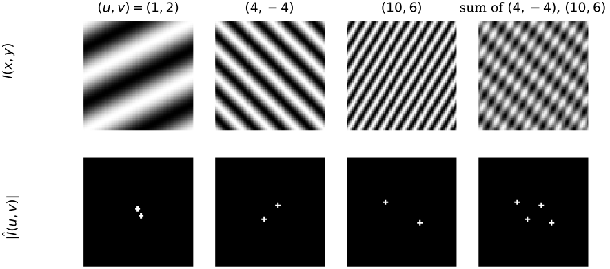
Top: plane waves \(\cos(2\pi(ux/64+vy/64))\) on a \(64\times64\) grid, and the average of the second and third. Bottom: their centred magnitude spectra. Each cosine is a symmetric pair of dots; a sum of two patterns is four dots. Finer stripes sit further from the centre.

Example (A 2 by 2 DFT by hand)

Take the image with top row \(1,2\) and bottom row \(3,4\). With \(N=M=2\) every exponential is \(e^{-i\pi ux}=(-1)^{ux}\), so each coefficient is a signed sum of the pixels:

\begin{align} \hat I(0,0)&=1+2+3+4=10\\ \hat I(1,0)&=1-2+3-4=-2\\ \hat I(0,1)&=1+2-3-4=-4\\ \hat I(1,1)&=1-2-3+4=0 \end{align}

Read the four lines as the total intensity, the left column minus the right, the top row minus the bottom, and the checkerboard pattern. The inverse at \((0,0)\) gives \(\tfrac14(10-2-4+0)=1\), as it should. The vertical step (2 per row) is twice the horizontal one (1 per column) and the spectrum says so; there is no checkerboard in the image.

Every coefficient depends on every pixel, so a spectrum describes the whole image, not a location. Computed directly the DFT costs \(O((MN)^2)\); the fast Fourier transform (FFT) gives the same numbers in \(O(MN\log MN)\), fastest when the sides are powers of two. The 2D transform is separable, \(e^{-i2\pi(ux+vy)}=e^{-i2\pi ux}e^{-i2\pi vy}\): transform every row, then every column.

the spectrum of a real image

centring

Plot \(\log(1+\lvert\hat I\rvert)\) for a photograph straight out of np.fft.fft2 and it looks like grey noise. The reason is bookkeeping. The DFT is periodic, \(\hat I(u+N,v)=\hat I(u,v)\), so index \(N-1\) is really frequency \(-1\): the low frequencies sit in the four corners of the array and the highest ones in the middle. Centring rolls the array by half its size so that zero frequency is in the middle and frequency grows outwards.

Proposition (Properties of the DFT)

For a real \(M\times N\) image \(I\) with DFT \(\hat I\):

(a) DC term: \(\hat I(0,0)=\sum_{x,y}I(x,y)=MN\,\bar I\), with \(\bar I\) the mean grey value.
(b) Implicit wrapping: the inverse formula evaluated outside the image gives \(I(x+N,y)=I(x,y+M)=I(x,y)\). The DFT treats the image as one tile of an infinite periodic pattern.
(c) Conjugate symmetry: \(\hat I(-u,-v)=\hat I^*(u,v)\), so the magnitude is symmetric about the origin.
(d) Shift: a circular shift by \((x_0,y_0)\) multiplies \(\hat I(u,v)\) by \(e^{-i2\pi(ux_0/N+vy_0/M)}\), a pure phase factor.
(e) Centring: for even \(M,N\), \(I(x,y)(-1)^{x+y}\) has DFT \(\hat I(u-N/2,\,v-M/2)\).

Property (e) is the shift theorem with \(u_0=N/2\), \(v_0=M/2\): the phase factor \(e^{i2\pi(\frac N2\frac xN+\frac M2\frac yM)}=e^{i\pi(x+y)}\) is exactly the checkerboard \((-1)^{x+y}\). For odd sizes the half-shift is not a whole number of samples; use np.fft.fftshift, which rolls by \(\lfloor N/2\rfloor\).

the bright cross

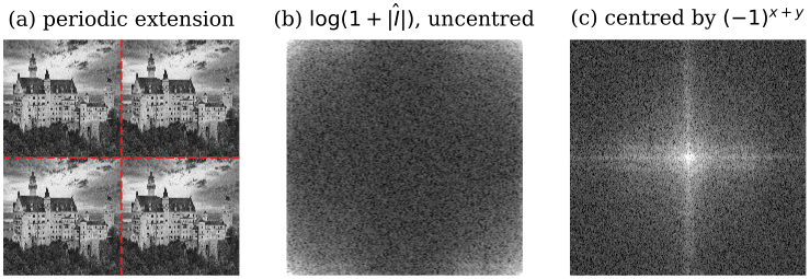
The averaged castle image. (a) The periodic image the DFT actually works on; dashed lines are the seams where the bottom row meets the top and the right column meets the left. (b) \(\log(1+\lvert\hat I\rvert)\) as computed, zero frequency at the corners. (c) Centred: energy piles up in the middle, and a bright cross runs through it.

Example (Reading the castle spectrum)

The DC term is \(\hat I(0,0)=124\,910.31=512^2\times0.4765\), the pixel count times the mean grey value, and conjugate symmetry holds to \(2\times10^{-12}\). Two features dominate the centred spectrum.

the bright centre: natural images are mostly slow shading and large shapes, so their energy is concentrated at low frequencies and falls off outwards.
the cross: it is not in the castle. Wrapping (property (b)) puts the dark trees of the bottom row directly above the bright sky of the top row. A horizontal seam is a sharp vertical jump, and a jump needs every vertical frequency \(v\) at \(u=0\): the vertical arm. The left/right seam gives the horizontal arm.

The cross is the spectral signature of the wrapping border mode. In the spatial picture the same thing looks like this: wrapping joins the top of a tower to its own base.

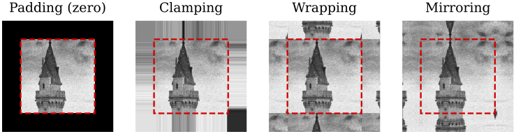
A \(96\times96\) crop expanded by 24 pixels in each border mode (dashed square: the original border). Padding draws a dark frame, clamping smears the edge pixels into streaks, wrapping copies the opposite side, mirroring continues the image smoothly. The DFT always uses wrapping.

magnitude versus phase

The magnitude spectrum is what everyone plots; the phase looks like random noise and is usually thrown away. It is the more important half. The shift property says that moving the image changes only the phase, so the phase is where the positions of all the edges live. Swapping the two halves between images makes the point.

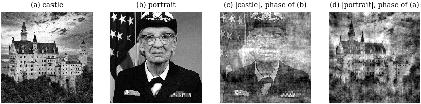
(c) The magnitude of the castle with the phase of the portrait; (d) the reverse. Each hybrid looks like the image whose phase it carries.

Example (Phase swap)

Hybrid (c) correlates \(0.765\) with the portrait (its phase) and only \(0.168\) with the castle (its magnitude); hybrid (d) correlates \(0.765\) with the castle and \(0.088\) with the portrait. The magnitudes of natural images are all roughly alike, bright at the centre and falling off outwards, so swapping them changes little beyond contrast and texture. Phase says where the structure is.

So the magnitude spectrum is a good place to look for things (periodic patterns, dominant orientations, what a filter removed), but it cannot be edited freely: any filter whose response is not real and symmetric about the centre changes the phase too and moves structure around.

the convolution theorem

Discrete convolution lays a flipped kernel over every pixel and sums: \[ (I*h)(x,y)=\sum_{i=-a}^{a}\sum_{j=-b}^{b} I(x-i,\,y-j)\,h(i,j). \] The flip is what makes filtering a single bright pixel reproduce the kernel itself, and it is what makes the theorem below hold. (Most libraries, OpenCV’s filter2D included, actually compute the unflipped correlation; for symmetric kernels the two agree.)

Theorem (Convolution theorem)

Convolution in one domain is multiplication in the other: \(\mathcal F\{I*h\}=\hat I\,\hat h\) and \(\mathcal F\{I\,h\}=\hat I*\hat h\). For \(M\times N\) arrays (the kernel zero-padded to the image size) the discrete statement holds for circular convolution, with indices taken modulo the image size: \[ \mathcal F\{I\circledast h\}(u,v)=\hat I(u,v)\,\hat h(u,v). \]

proof: convolution theorem

Proof (Convolution theorem)

In one dimension (the 2D case repeats each step in \(y\)), with all indices modulo \(N\):

\begin{align} \mathcal F\{I\circledast h\}(u) &= \sum_x\sum_{x’} I(x’)\,h(x-x’)\,e^{-i2\pi ux/N} \\ &= \sum_{x’} I(x’)\,e^{-i2\pi ux’/N}\sum_x h(x-x’)\,e^{-i2\pi u(x-x’)/N} \\ &= \sum_{x’} I(x’)\,e^{-i2\pi ux’/N}\;\hat h(u) = \hat I(u)\,\hat h(u). \end{align}

The second line splits the exponential as \(e^{-i2\pi ux’/N}e^{-i2\pi u(x-x’)/N}\). In the third, \(x-x’\) runs over one full period as \(x\) does, so the inner sum is \(\hat h(u)\) whatever \(x’\) is. The continuous case is the same computation with integrals over \(\mathbb R\).

circular, not linear

The theorem is about the DFT’s convolution, which wraps. Multiplying two spectra and inverting filters the periodically extended image, seams and all.

Example (Circular against linear convolution)

Take \(I=(1,2,3,4)\) and \(h=(1,1,0,0)\), so \((I\circledast h)(x)=I(x)+I(x-1)\) with \(x-1\) taken modulo 4: \[ I\circledast h=(1+4,\;2+1,\;3+2,\;4+3)=(5,3,5,7). \] Through the DFT: \(\hat I=(10,\,-2+2i,\,-2,\,-2-2i)\), \(\hat h=(2,\,1-i,\,0,\,1+i)\), product \((20,\,4i,\,0,\,-4i)\), and the inverse DFT returns \((5,3,5,7)\). The zero-padded (linear) convolution is \((1,3,5,7,4)\): the first output differs because \(5=1+4\) treats \(I(3)\) as the left neighbour of \(I(0)\).

To get linear convolution from the FFT, zero-pad image and kernel to at least \((M+k-1)\times(N+k-1)\) before transforming, so the wrapped contributions land on zeros.

filtering by multiplication

Definition (Algorithm: frequency-domain filtering)

Input: an image \(I\) of even size \(M\times N\) and a centred filter \(\hat h(u,v)\) of the same size, real and symmetric about the centre.

Centre: \(I_c(x,y)=I(x,y)\,(-1)^{x+y}\).
Transform: \(\hat I=\mathrm{FFT}(I_c)\).
Filter: \(\hat J(u,v)=\hat I(u,v)\,\hat h(u,v)\), value by value.
Invert: \(g=\mathrm{FFT}^{-1}(\hat J)\) and keep its real part (the imaginary part is rounding error, about \(10^{-16}\)).
Undo the centring: \(J(x,y)=\operatorname{Re}g(x,y)\,(-1)^{x+y}\).

Cost: two FFTs and \(MN\) multiplications, whatever the size of the equivalent spatial kernel.

Step 4 is safe only because the filter is real and symmetric: a real image has a conjugate-symmetric spectrum, multiplying by such a filter preserves that symmetry, and the inverse of a conjugate-symmetric array is real. A filter that keeps only positive \(u\), say, gives a genuinely complex output, and dropping the imaginary part then throws information away.

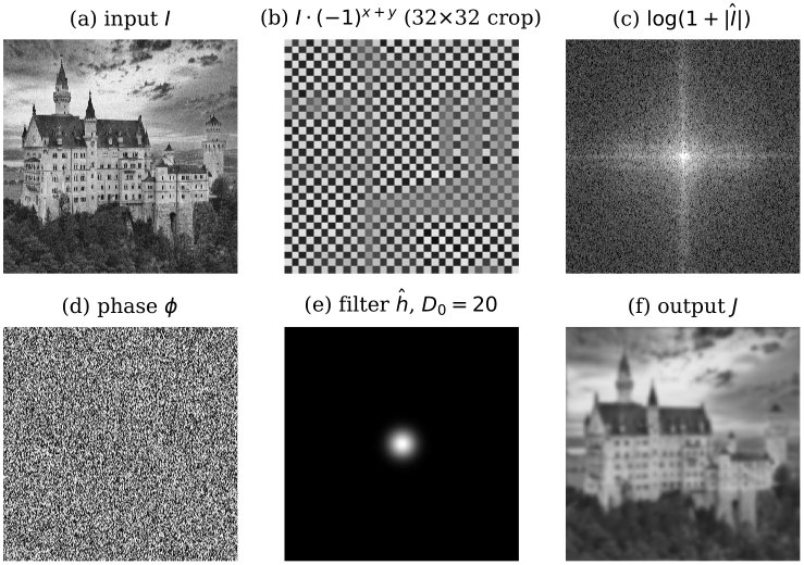
The algorithm on the castle image. (a) Input. (b) After centring (a \(32\times32\) crop showing the sign alternation). (c) Magnitude and (d) phase of the centred DFT. (e) Gaussian low-pass filter, \(D_0=20\). (f) Output: a blurred castle.

Example (Gaussian low-pass on the castle)

The filter is \(\hat h(u,v)=\exp(-(u’^2+v’^2)/(2D_0^2))\) with \((u’,v’)\) the offset from the centre and \(D_0=20\) frequency samples. It keeps \(95.8\%\) of the spectral energy, most of it (\(81.0\%\) of the total) the DC term alone; \(\hat h=1\) at the centre, so the mean grey value \(0.4765\) is unchanged. The output agrees with a spatial Gaussian blur of \(\sigma=N/(2\pi D_0)=4.074\) pixels, wrapping borders, to \(7\times10^{-16}\): by the convolution theorem these are the same operation.

Low-pass filters keep the centre of the spectrum and blur; high-pass filters keep the outside, \(\hat h_{\text{hp}}=1-\hat h_{\text{lp}}\), which is the image minus its blurred self (the detail layer of unsharp masking); band-pass filters keep a ring.

Example (When is the FFT route cheaper?)

Count complex multiplications for a \(512\times512\) image, with \(N^2\log_2N\) per 2D FFT: \[ \text{FFT route}\approx 3\cdot512^2\cdot9+512^2=7\,340\,032 \] (image, kernel and inverse FFTs, plus the product), against \(512^2k^2\) for a direct \(k\times k\) kernel: \(6\,553\,600\) at \(k=5\), \(251\,920\,384\) at \(k=31\). The FFT route wins from about \(k=6\) and is 34 times cheaper at \(k=31\). A complex multiplication costs about four real ones, which moves the break-even to about \(k=11\). A separable kernel costs only \(2k\) per pixel, \(16\,252\,928\) at \(k=31\), so a Gaussian is still best done in the spatial domain.

Remark (When frequency-domain filtering fails)

wrapping: without zero padding, the border seams leak into the output.
ringing: an ideal low-pass (1 inside a disc, 0 outside) has an oscillating spatial kernel and rings next to every edge. The Gaussian has no ripples in either domain.
nonlinear filters: the median filter has no \(\hat h\) at all.
non-periodic noise: random noise overlaps the image’s own frequencies, so a fixed \(\hat h\) cannot remove it without removing detail too.

Use it for large non-separable kernels (above \(k\approx11\)), for filters that are naturally stated in frequency (notch, band-pass), and to understand what a filter does. For small or separable kernels, filter in the spatial domain.

notch filtering a periodic artefact

A periodic artefact (scanline stripes from a satellite sensor, mains-hum interference) is a sum of a few plane waves. In the image it is spread over every pixel and tangled with the content; in the spectrum it is a few bright, isolated dots placed symmetrically about the centre. Delete the dots and the artefact is gone, while the rest of the image, whose energy is spread smoothly, barely notices.

Definition (Algorithm: notch-reject filtering)

Compute the centred log spectrum \(\log(1+\lvert\hat I\rvert)\) and locate the artefact’s peaks \(\pm(u_k,v_k)\): isolated spikes away from the centre, in symmetric pairs.
Build the notch-reject filter as a product of inverted Gaussian notches, \[ \hat h_{\text{NR}}(u,v)=\prod_k\Bigl(1-e^{-d_k(u,v)^2/(2r^2)}\Bigr), \] with \(d_k\) the distance to the \(k\)-th peak and \(r\) a few samples. Include both members of every pair, so the filter stays symmetric and the output stays real.
Run the frequency-domain filtering algorithm with \(\hat h_{\text{NR}}\).
Optionally, filter with the notch-pass \(1-\hat h_{\text{NR}}\) to see the artefact on its own and check that nothing else was removed.

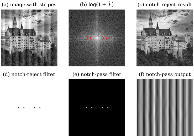
(a) The castle with added vertical stripes. (b) Its centred log spectrum; the four stripe spikes are circled. (c) Notch-reject result. (d) The notch-reject filter, black dots on white. (e) The notch-pass filter. (f) Notch-pass output: the stripes alone.

Example (Removing stripes)

The stripes are \[ 0.1\sin(2\pi\cdot48x/512)+0.05\sin(2\pi\cdot96x/512), \] with periods \(10.7\) and \(5.3\) pixels. They vary only along \(x\), so \(v=0\) and the spectrum gains four spikes on the horizontal axis, at \(u=\pm48\) and \(u=\pm96\). Four Gaussian notches with \(r=3\) zero just \(0.09\%\) of the frequency plane. The RMS difference from the clean image falls from \(0.0791\) to \(0.0077\), and the notch-pass output reproduces the stripes with the same error \(0.0077\). That residual is the castle’s own content at the notched frequencies, removed along with the artefact.

Remark (When notch filtering fails)

It needs the artefact’s energy to sit in a few isolated spikes. Random noise is spread across the whole spectrum and has no spike to delete. The peaks must be found, by eye or by peak-finding away from the centre, and notches that are too wide, or placed near the centre where the image’s own energy is, delete real structure. Use notches for stripes, scanlines and mains interference; for random noise use a Gaussian low-pass or a median filter instead.

the difference of Gaussians as a band-pass filter

the Gaussian is its own transform

Proposition (The Fourier transform of a Gaussian)

For the normalised Gaussian of width \(\sigma\), \[ G_\sigma(x,y)=\frac{1}{2\pi\sigma^2}e^{-\frac{x^2+y^2}{2\sigma^2}} \quad\longleftrightarrow\quad \hat G_\sigma(u,v)=e^{-2\pi^2\sigma^2(u^2+v^2)}, \] a Gaussian of width \(\sigma_u=1/(2\pi\sigma)\) in frequency. A wide kernel is a narrow low-pass filter, and the reverse.

That is why the Gaussian is the default smoothing kernel: no ripples in either domain, so it blurs without ringing (a box filter’s transform is an oscillating sinc). Its response falls to one half at \(u=0.187/\sigma\) cycles per pixel. On a DFT grid of \(N\) samples a frequency-domain Gaussian of width \(D_0\) samples is a spatial one with \(\sigma=N/(2\pi D_0)\), the \(4.074\) pixels of the low-pass example.

proof: Gaussian transform

Proof (The Fourier transform of a Gaussian)

In one dimension, complete the square in the exponent: \[ -\frac{x^2}{2\sigma^2}-i2\pi ux=-\frac{(x+i2\pi\sigma^2u)^2}{2\sigma^2}-2\pi^2\sigma^2u^2. \] The factor \(e^{-2\pi^2\sigma^2u^2}\) comes out of the integral, and what remains is a shifted normalised Gaussian, which integrates to 1. The 2D Gaussian is a product of 1D Gaussians in \(x\) and \(y\), and the transform of such a product is the product of the 1D transforms.

the difference of Gaussians

Subtract a wide blur from a narrow one. The narrow blur keeps everything except pixel-level noise; the wide one keeps only the slow shading; their difference keeps what lies between: edges and texture at one scale.

Definition (Difference of Gaussians)

For \(\sigma_1<\sigma_2\), by linearity of the transform, \[ \mathrm{DoG}=G_{\sigma_1}-G_{\sigma_2} \quad\longleftrightarrow\quad \widehat{\mathrm{DoG}}(u,v)=e^{-2\pi^2\sigma_1^2(u^2+v^2)}-e^{-2\pi^2\sigma_2^2(u^2+v^2)}. \] In space it is a narrow positive peak in a wide negative trough, an approximation to the inverted Laplacian of Gaussian. Filtering with it equals subtracting the two blurred images, \(I*(G_{\sigma_1}-G_{\sigma_2})=I*G_{\sigma_1}-I*G_{\sigma_2}\), by distributivity.

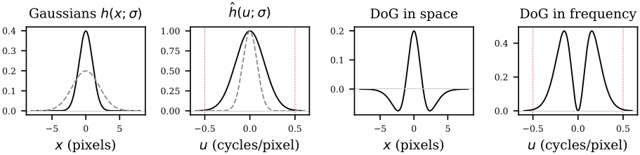
From left: Gaussians with \(\sigma=1\) (solid) and \(\sigma=2\) (dashed); their transforms; the DoG \(G_1-G_2\) in space; and in frequency, where it is zero at \(u=0\), peaks at \(u^*=0.153\) and has nearly died by the Nyquist frequency \(\pm0.5\) (dotted red).

The response is \(0\) at \(u=0\) (the kernel sums to zero, so flat regions map to zero) and tends to \(0\) as \(u\to\infty\) (both Gaussians vanish). So the DoG is a band-pass filter, not the high-pass filter it is often drawn as. Setting the derivative of the 1D response to zero locates its peak: \[ u^*=\sqrt{\frac{\ln(\sigma_2^2/\sigma_1^2)}{2\pi^2(\sigma_2^2-\sigma_1^2)}}. \] For \(\sigma_1=1\), \(\sigma_2=2\) pixels, \(u^*=0.153\) cycles per pixel with height \(0.472\), and the response at Nyquist is only \(0.007\). It behaves like a true high-pass only when \(\sigma_1\) is so small that \(G_{\sigma_1}\) is nearly an impulse, giving \(1-\hat G_{\sigma_2}\).

proof: why it approximates the Laplacian of Gaussian

Proposition (The DoG is a scaled, inverted Laplacian of Gaussian)

For \(\sigma_2\) close to \(\sigma_1\), \(G_{\sigma_1}-G_{\sigma_2}\approx-(\sigma_2-\sigma_1)\,\sigma\nabla^2G_\sigma\).

Proof (The DoG is a scaled, inverted Laplacian of Gaussian)

Differentiate the Gaussian’s transform with respect to its width: \[ \frac{\partial}{\partial\sigma}e^{-2\pi^2\sigma^2u^2}=-4\pi^2\sigma u^2\,e^{-2\pi^2\sigma^2u^2}=\sigma\,(i2\pi u)^2\,\hat G_\sigma(u). \] Differentiation in space multiplies the transform by \(i2\pi u\), so the right side is the transform of \(\sigma G_\sigma’’\), or \(\sigma\nabla^2G_\sigma\) in 2D. A finite difference in \(\sigma\) then gives the claim. The same multiplication by \(i2\pi u\) is why derivative filters amplify noise: their gain grows without bound in \(u\), and a Gaussian factor is what brings it back down.

worked example: the Lab 1 DoG

Example (Frequency response of a binomial DoG)

Lab 1 builds a DoG from binomial kernels: \(h_1\) the \(3\times3\) kernel \(\tfrac1{16}(1,2,1)^\top(1,2,1)\) zero-padded to \(5\times5\), and \(h_2=\tfrac1{256}(1,4,6,4,1)^\top(1,4,6,4,1)\). Its response is exact. The 1D kernel \(\tfrac14(1,2,1)\) has transform \[ \tfrac14\bigl(e^{i2\pi u}+2+e^{-i2\pi u}\bigr)=\tfrac12(1+\cos2\pi u)=\cos^2(\pi u), \] the 1D kernel \(\tfrac1{16}(1,4,6,4,1)\) has transform \(\cos^4(\pi u)\), and so \[ \hat h_1-\hat h_2 = t-t^2, \qquad t=\cos^2(\pi u)\cos^2(\pi v)\in[0,1]. \] The second transform uses the convolution theorem, since \(\tfrac1{16}(1,4,6,4,1)=\tfrac14(1,2,1)*\tfrac14(1,2,1)\); the last step uses separability. The response is 0 at \(t=1\) (only at \(u=v=0\): DC removed) and at \(t=0\) (wherever \(u\) or \(v\) is \(\pm\tfrac12\): the highest frequencies removed). It peaks at \(\tfrac14\) where \(t=\tfrac12\), for example at \((\pm\tfrac14,0)\). The \(5\times5\) kernel’s DFT matches this formula to \(3\times10^{-16}\).

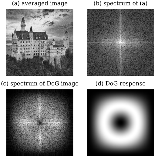
(a) The averaged castle. (b) Its centred spectrum. (c) The spectrum of the DoG-filtered image: a dark centre. (d) The DoG’s response \(t-t^2\), a ring (white is \(0.25\), black \(0\)).

The two spectra say what the filter did. The averaged image has DC magnitude \(124\,910\) and \(84.4\%\) of its non-DC energy below \(0.05\) cycles per pixel; the DoG image has DC exactly 0, only \(0.5\%\) of its energy below \(0.05\), and \(33.3\%\) above \(0.25\) (against \(3.5\%\) for the original). The sky and the overall brightness are gone; the edges and texture remain, exactly where the ring says.

Remark (When the DoG fails, and what to use instead)

A DoG answers to one band, set by \(\sigma_1\) and \(\sigma_2\): structures much finer or coarser are missed, so the widths must match the edges or blobs sought, or a stack of DoGs is needed (the scale space of SIFT). With unequal weights on the two Gaussians the response at \(u=0\) is not zero and shading leaks through.

versus the \(3\times3\) Laplacian: prefer the DoG on noisy images; it suppresses the highest frequencies that the Laplacian amplifies.
versus an explicit Laplacian of Gaussian: prefer the DoG when speed matters; it is two separable Gaussian blurs and a subtraction.

Gaussian and Laplacian pyramids

Different structures live at different scales. Fine detail needs full resolution; large objects can be found more cheaply, and with a smaller kernel, at low resolution. Since an image usually holds both, keep it at several resolutions at once: a pyramid, each level half the rows and columns of the one below. The aliasing figure at the top of the page is the reason each level must be low-pass filtered before it is subsampled.

Definition (Gaussian and Laplacian pyramids)

Let \(I_0=I\), \(h_a\) a small low-pass approximation filter (Gaussian or binomial) and \(h_i\) an interpolation filter. With \(\downarrow2\) keeping every second row and column and \(\uparrow2\) inserting zeros between samples: \[ I_{j+1}=(I_j*h_a)\downarrow2, \qquad P_j=(I_{j+1}\uparrow2)*h_i, \qquad R_j=I_j-P_j. \] \(I_0,\dots,I_J\) is the Gaussian (approximation) pyramid. The residuals \(R_0,\dots,R_{J-1}\) together with the top \(I_J\) form the Laplacian (prediction-residual) pyramid. Each \(R_j\) is an image minus a smoothed version of itself, a DoG-like band-pass image; hence the name.

Definition (Algorithm: build and reconstruct)

Build, for \(j=0,\dots,J-1\):

Approximate: \(I_{j+1}\gets(I_j*h_a)\downarrow2\).
Predict: \(P_j\gets(I_{j+1}\uparrow2)*h_i\).
Store the residual: \(R_j\gets I_j-P_j\).

Reconstruct: start from \(\tilde I\gets I_J\) and for \(j=J-1,\dots,0\) set \(\tilde I\gets(\tilde I\uparrow2)*h_i+R_j\). The result is \(I\) exactly.

Cost: each level has a quarter of the pixels of the one below, so building costs about \(\tfrac43\) of one filtering pass over the base, and storage is about \(\tfrac43N^2\) values.

Proposition (Reconstruction is exact)

For any filters \(h_a\) and \(h_i\), the reconstruction loop returns \(I\) exactly.

The reason is one line, by induction down from the top: if \(\tilde I=I_{j+1}\) before step \(j\), then \((\tilde I\uparrow2)*h_i+R_j=P_j+(I_j-P_j)=I_j\). The residual stores exactly what the prediction misses. The filters only decide how good the prediction is, and so how small the residuals are. The gain of a Laplacian pyramid is not size (it is a third larger than the image) but statistics: residuals are mostly near zero, so they compress well, and each level isolates one band of frequencies.

Example (One pyramid level by hand)

Take \(I_0=(0,4,8,8,8,4,0,0)\), \(h_a=\tfrac14(1,2,1)\), \(h_i=\tfrac12(1,2,1)\) (linear interpolation) and mirrored borders. Smoothing gives, for example, \(\tfrac14(4+2\cdot8+8)=7\) at position 2: \[ I_0*h_a = (2,\,4,\,7,\,8,\,7,\,4,\,1,\,0). \] Keeping positions \(0,2,4,6\) gives \(I_1=(2,\,7,\,7,\,1)\). Upsampling with \(h_i\) turns each inserted sample into the mean of its neighbours: \[ P_0 = (2,\,4.5,\,7,\,7,\,7,\,4,\,1,\,1), \] \[ R_0 = I_0-P_0 = (-2,\,-0.5,\,1,\,1,\,1,\,0,\,-1,\,-1). \] \(P_0+R_0=I_0\). The residual is small on the plateau and largest at the corners of the profile, which the prediction rounds off.

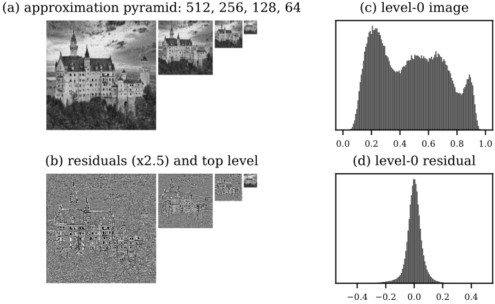
(a) Gaussian pyramid of the castle: 512, 256, 128 and 64 pixels wide. (b) The Laplacian residuals of levels 0 to 2 (contrast stretched about mid-grey) and the \(64\times64\) top, which together rebuild the image exactly. (c) The image’s grey-value histogram, broad and bimodal. (d) The level-0 residual’s histogram, a spike at zero.

Example (Pyramids of the castle)

With the \(5\times5\) binomial kernel as \(h_a\) and four times it as \(h_i\) (the factor 4 makes up for the three zeros inserted per kept sample), three reduction steps give residuals that are edge maps: grey almost everywhere, structure only at edges and texture. Their standard deviation is \(0.058\) against \(0.231\) for the image, and \(72.4\%\) of level-0 residuals are below \(0.05\) in absolute value. The pyramid holds \(348\,160\) values against \(262\,144\) (\(1.328\) times as many) and reconstructs the image to \(7\times10^{-17}\).

Remark (When pyramids fail, and when to use them)

aliasing: if \(h_a\) smooths too little, the coarse levels alias.
awkward sizes: the image must be divisible by \(2^J\), or be padded or cropped.
coarse scale steps: scale is sampled only in factors of 2, too coarse for objects whose size falls between levels; SIFT uses several blurs per octave instead.
no shift invariance: subsampling means a one-pixel shift of the input can change the coarse residuals noticeably.

Use a Gaussian pyramid for coarse-to-fine search and for finding objects of unknown size with one fixed-size detector; use a Laplacian pyramid for compression and for blending two images band by band.

what to remember

filter	keeps	removes	example
low-pass	centre of spectrum	edges, noise	Gaussian blur
high-pass	outside	shading	image minus blur
band-pass	a ring	shading and noise	DoG, pyramid level
notch	all but a few dots	periodic artefacts	stripe removal

The DFT wraps the image; that is the cross in every photograph’s spectrum, and the reason FFT filtering needs zero padding to match ordinary convolution.
Magnitude ignores translation; position lives in the phase.
The median filter has no frequency response: it is nonlinear.
Every Gaussian-pyramid level is a low-pass image; every Laplacian-pyramid level except the top is a band-pass residual.

Further reading: Szeliski, Computer Vision: Algorithms and Applications (2nd ed.), §3.4 on Fourier transforms and §3.5 on pyramids and blending.

Seeing in Frequency

aliasing: why frequency is the right language

images as sums of waves