Morphology: Counting Nuts and Bolts
A threshold almost never hands you a clean mask. You get specks of noise in the background, pinholes and cracks in the objects, ragged edges, objects cut off by the frame and objects that touch. Mathematical morphology is the toolkit for repairing such masks. It treats a binary image as a set of pixels and probes it with a small set of offsets. Everything is built from two primitives, one that grows objects and one that shrinks them, together with plain set algebra. There are no derivatives and no weights: the operations are nonlinear, and they judge structures by size and shape rather than by contrast.
This page builds the toolkit and then uses it on a single task: count the nuts and bolts in a photo, and say whether the batch needs parts added or removed. Each tool earns its place by fixing one specific failure of that pipeline. Thresholding and connected components, the steps before and after morphology, are on the Classical Segmentation page. Further reading: Szeliski (2nd ed.) §3.3.3.
sets and structuring elements
A binary image is the set of its foreground pixels, \(I=\{\mathbf x\in\mathbb Z^2 : \mathbf x \text{ is foreground}\}\), with \(\mathbf x=(x,y)\), \(x\) the column and \(y\) the row. On images, union is OR, intersection is AND, complement \(I^c\) is NOT and difference \(A-B=A\cap B^c\) is AND NOT. Two further operations are geometric: the translate \(A_{\mathbf x}=\{\mathbf a+\mathbf x : \mathbf a\in A\}\) and the reflection \(A^r=\{-\mathbf a : \mathbf a\in A\}\).
A structuring element \(S\subseteq\mathbb Z^2\) is a small set of offsets with a designated origin. The default is the \(3\times3\) square \(S_{3\times3}=\{-1,0,1\}^2\). Other common choices are the cross (the origin and its four edge neighbours), digital discs, lines, and asymmetric shapes.
The shape of \(S\) decides two things. It sets the connectivity: the square is 8-connected and the cross is 4-connected. It also gets stamped onto every result, so a big square turns round outlines into straight-edged ones. Use a disc whenever you plan to measure shape afterwards.
dilation and erosion
Slide \(S\) over the image. Dilation asks at each position whether \(S\) hits the object; erosion asks whether it fits inside it. Hitting adds a layer of pixels around every object, and fitting peels a layer off.
\[ I\oplus S=\{\mathbf x : S^r_{\mathbf x}\cap I\neq\emptyset\},\qquad I\ominus S=\{\mathbf x : S_{\mathbf x}\subseteq I\}. \] Equivalently, as unions and intersections of shifted copies of the image, \[ I\oplus S=\bigcup_{\mathbf s\in S} I_{\mathbf s},\qquad I\ominus S=\bigcap_{\mathbf s\in S} I_{-\mathbf s}. \]
The second form is the one to remember. Dilation is an OR of shifts: stamp a copy of \(S\) at every object pixel, which makes it the Minkowski sum. Erosion is an AND of shifts. With the \(3\times3\) square, dilation turns on every background pixel that has an object pixel among its eight neighbours, and erosion keeps only the object pixels whose eight neighbours are all object. The reflection in the definition is what makes “hits” equal “stamp”. It is invisible for symmetric elements (square, cross, disc) and matters only for lopsided ones: an element made of the origin and its right neighbour grows every horizontal run by one pixel on the right, and erosion by it trims one pixel off the right.
The consequences follow directly from the definitions:
- dilation fills holes and gaps narrower than \(S\), and can merge nearby objects;
- erosion deletes objects and protrusions narrower than \(S\), and can split an object at a thin neck.
Take the image in the top-left panel below: a \(3\times3\) block, a two-pixel spur hanging off its corner and one isolated pixel, 12 pixels in all, with \(S=S_{3\times3}\).
- Dilation. Each of the 12 pixels stamps a \(3\times3\) square. The union is one connected 38-pixel object, so 26 pixels are added. The isolated pixel has been absorbed into the main object.
- Erosion. A pixel survives only if its whole \(3\times3\) neighbourhood is foreground. Only the centre of the block qualifies, so \(|I\ominus S|=1\). The spur and the isolated pixel, both thinner than \(S\), vanish.
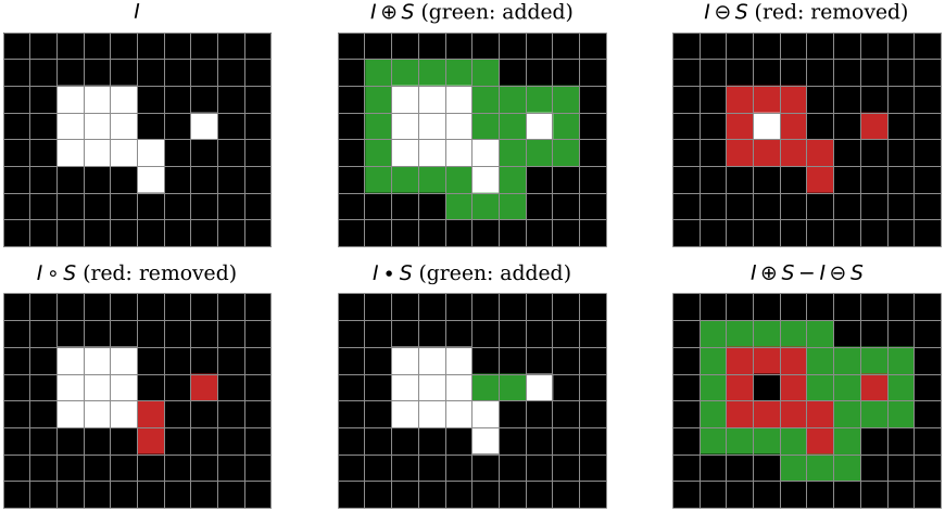
Binary morphology on a small grid with the \(3\times3\) square. Green pixels are added to \(I\), red pixels removed. The bottom right panel is the morphological edge \((I\oplus S)-(I\ominus S)\): outer edge green, inner edge red.
Large elements are cheap because shifts add. Dilating by \(S_1\oplus S_2\) is the same as dilating by \(S_1\) and then by \(S_2\), and the same holds for erosion. A \(9\times9\) square is the \(3\times3\) square dilated by itself three times, so a \(9\times9\) erosion costs four \(3\times3\) passes, 36 look-ups per pixel instead of 81. Splitting each \(3\times3\) pass into a row and a column brings that down to 24. This is the separable-kernel trick from linear filtering, with OR (or max) in place of the weighted sum.
Pixels outside the image need a value. Treating them as background, the usual choice, makes erosion eat into objects that touch the frame.
proofs
\[ I\oplus S=\{\mathbf a+\mathbf s : \mathbf a\in I,\ \mathbf s\in S\}=\bigcup_{\mathbf s\in S}I_{\mathbf s}, \] and \(I\oplus(S_1\oplus S_2)=(I\oplus S_1)\oplus S_2\), \(I\ominus(S_1\oplus S_2)=(I\ominus S_1)\ominus S_2\).
Since \(S^r_{\mathbf x}=\{\mathbf x-\mathbf s : \mathbf s\in S\}\), we have \(\mathbf x\in I\oplus S\) iff some \(\mathbf a\in I\) equals \(\mathbf x-\mathbf s\) for some \(\mathbf s\in S\), that is, iff \(\mathbf x=\mathbf a+\mathbf s\).
For the decomposition of dilation, \((I\oplus S_1)\oplus S_2=\{\mathbf a+\mathbf s_1+\mathbf s_2\}\), which is \(I\oplus(S_1\oplus S_2)\) by associativity of vector addition. For erosion, \(\mathbf x\in(I\ominus S_1)\ominus S_2\) iff \(\mathbf x+\mathbf s_2+\mathbf s_1\in I\) for every \(\mathbf s_1\in S_1\) and \(\mathbf s_2\in S_2\). The sums \(\mathbf s_1+\mathbf s_2\) are exactly the elements of \(S_1\oplus S_2\), so this says \((S_1\oplus S_2)_{\mathbf x}\subseteq I\).
opening and closing
Dilation and erosion both change the size of every object. Composing them with the same element undoes most of the size change but keeps the removal of small detail.
\[ I\circ S=(I\ominus S)\oplus S,\qquad I\bullet S=(I\oplus S)\ominus S. \] Opening (erode, then dilate) removes foreground detail smaller than \(S\): specks, spurs and thin bridges. Closing (dilate, then erode) removes background detail smaller than \(S\): pinholes, cracks and narrow gaps.
The cleanest picture of opening: it is the union of all translates of \(S\) that fit inside \(I\). Roll the element around inside the object; whatever it cannot reach is removed. Closing does the same thing to the background.
For any \(I\) and \(S\):
- \(I\circ S=\bigcup\{S_{\mathbf x} : S_{\mathbf x}\subseteq I\}\), so \(I\circ S\subseteq I\): opening never adds pixels;
- \(I\subseteq I\bullet S\): closing never removes pixels;
- both are idempotent, so opening twice is the same as opening once;
- they are dual: \((I\bullet S)^c=I^c\circ S^r\). Closing the objects is opening the background.
Idempotence is what makes these operations filters rather than mere transformations. Once a structure has survived an opening by \(S\), it survives every later opening by \(S\). The name also tells you which is which, because it describes what happens to the background: opening opens the background up into the object, so thin parts of the object disappear, while closing closes background gaps inside the object.
Same image, same \(S\) as before (middle panels of the figure above).
- Opening. The erosion left one pixel, the centre of the block. Dilating that pixel gives back the whole block, so \(|I\circ S|=9\). The spur and the isolated pixel are gone, the block is untouched, and 3 pixels have been removed.
- Closing. Eroding the 38-pixel dilation removes all the added pixels except the two that bridge the one-pixel gap between the block and the isolated pixel. So \(|I\bullet S|=14\): the gap is sealed.
| operation | removes | typical target | risk |
|---|---|---|---|
| opening | foreground \(<S\) | specks, spurs | splits at necks |
| closing | background \(<S\) | pinholes, cracks | merges across gaps |
Assuming \(S\) contains the origin, \(I\ominus S\subseteq I\subseteq I\oplus S\), so three differences come for free. The outer edge \((I\oplus S)-I\) is the background pixels touching an object. The inner edge \(I-(I\ominus S)\) is the object pixels touching the background. The morphological edge \((I\oplus S)-(I\ominus S)\) is both. In the example these have \(26\), \(11\) and \(37\) pixels. Subtracting the other way round, for instance \((I\ominus S)-I\), always gives the empty set.
When it fails. Opening and closing judge detail only by its width relative to \(S\). If the noise and the structures you care about are equally thin (a wire next to specks of the same thickness), no choice of \(S\) removes one and keeps the other. Each operation also has a characteristic accident: opening splits objects joined by a thin neck, and closing merges objects separated by a narrow gap.
When to use it vs alternatives. Open to knock specks and spurs off a thresholded mask, and close to seal pinholes and cracks. When whole objects must be kept or removed according to where they are rather than how thick they are, for example objects touching the border or holes of any width, use reconstruction.
proofs
(1) \(\mathbf x\in I\ominus S\) means \(S_{\mathbf x}\subseteq I\). Dilating the set of such \(\mathbf x\) by \(S\) stamps \(S_{\mathbf x}\) at each of them, which gives exactly the union of the translates that fit. Each translate lies inside \(I\), so the union does too.
(4) First, erosion and dilation are dual: \(\mathbf x\notin I\ominus S\) iff some \(\mathbf x+\mathbf s\) lies in \(I^c\), iff \(S_{\mathbf x}\cap I^c\neq\emptyset\), iff \(\mathbf x\in I^c\oplus S^r\). So \((I\ominus S)^c=I^c\oplus S^r\), and in the same way \((I\oplus S)^c=I^c\ominus S^r\). Then \[ (I\bullet S)^c=\big((I\oplus S)\ominus S\big)^c=(I\oplus S)^c\oplus S^r=(I^c\ominus S^r)\oplus S^r=I^c\circ S^r . \]
(2) By (1), \(I^c\circ S^r\subseteq I^c\). Taking complements reverses the inclusion, and (4) turns the left side into \(I\bullet S\).
(3) \(I\circ S\) is a union of translates of \(S\), each of which still fits inside it, so by (1) opening it again returns it unchanged. Closing follows by duality.
morphological reconstruction
Opening and closing treat every object alike. Many tasks instead need to keep or delete whole objects according to where they are: the objects a user clicked on, the objects cut by the image border, the background regions that are really holes. Reconstruction does this. It starts from seed pixels and grows them one dilation at a time, never letting them leave the mask.
Given a mask \(I\) and a marker \(R_0\subseteq I\), iterate \[ R_i=(R_{i-1}\oplus S)\cap I \] until \(R_i=R_{i-1}\). The limit \(R\) consists of exactly those connected components of \(I\) that contain a seed. Connectivity here means the connectivity of \(S\): 8-connectivity for the square, 4-connectivity for the cross.
Why it works: \(S\) contains the origin, so the iterates only grow, and they stay inside the finite set \(I\), so the loop terminates. Each step adds exactly the mask pixels adjacent to the current set. The seeds therefore flood their own components and can never jump across background into another one. In practice this is a queue-based flood fill done in a single pass. The iterative form is the one to reason with, because it needs one pass per pixel of the longest path inside an object, plus one more to confirm that nothing changed. Two classic algorithms use the image border as the seed.
Input: binary image \(I\). Output: the objects of \(I\) that do not touch the border.
- \(M\leftarrow\) the foreground pixels of \(I\) in the first or last row or column.
- \(R\leftarrow\) the reconstruction of \(I\) from the marker \(M\).
- Return \(I-R\).
Input: binary image \(I\). Output: \(I\) with every hole filled.
- Form the complement \(I^c\), which is the background.
- \(M\leftarrow\) the pixels of \(I^c\) in the first or last row or column.
- \(R\leftarrow\) the reconstruction of \(I^c\) from \(M\), using the cross if the objects are 8-connected.
- Return \(R^c\).
Hole filling rests on one definition: a hole is background that cannot reach the border. Flood the background inwards from the frame, and whatever stays dry is either object or hole. Complementing the flood fills the holes. The choice of the cross in step 3 matters. An 8-connected outline can have diagonal steps, and an 8-connected flood would slip through those diagonal gaps into the hole. Pairing 8-connected objects with a 4-connected background is the standard fix for this connectivity paradox.
The \(9\times12\) image below has four objects and 30 pixels: \(A\) touching the left border, a square ring \(B\) of 16 pixels around a \(3\times3\) hole, \(C\) in the bottom-right corner, and a small square \(D\).
- One seed on the top of the ring, with the \(3\times3\) square. Each iteration spreads one pixel further round the ring in both directions. The far side of the ring is six steps away, so \(R_6=B\), \(R_7\) confirms it, and the result is the ring alone, whatever its shape.
- Border clearing. The marker is the 6 border pixels of \(A\) and \(C\). One dilation inside \(I\) covers both objects and the second changes nothing, so \(I-R=B\cup D\), which has 20 pixels.
- Hole filling. The background has 78 pixels. Flooding it from the border with the cross reaches everything except the 9 pixels inside the ring. Complementing gives \(I\) plus the hole, 39 pixels.
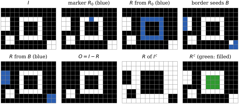
Reconstruction from one seed (top row, first three panels), border clearing (top right to bottom row, second panel), and hole filling (last two panels: the flooded background \(R\) of \(I^c\), and its complement, with the filled hole in green).
When it fails. Reconstruction works on whole connected components, so it inherits every segmentation error. An object fused to a border object by a one-pixel bridge is deleted along with it. A nut whose ring is broken by a crack has no hole to fill, because the crack lets the border flood in. A large hole whose outline touches the image border is, by definition, border-connected background, and is never filled. The remedy is to clean the mask with a closing or opening first, which is exactly the order the nuts-and-bolts pipeline uses.
When to use it vs alternatives. Use reconstruction whenever the decision is per object (keep, remove, fill) rather than per pixel. Opening cannot remove a large object just because it touches the border, and closing cannot fill a hole wider than \(S\).
the distance transform and touching objects
Erode an object over and over and record the iteration at which each pixel disappears. That record is a distance map, and the last pixels to go mark the object’s centres. Those centres are what lets us pull touching objects apart.
Set \(I_0=I\) and \(I_i=I_{i-1}\ominus S\) until \(I_i=\emptyset\). The distance transform is the grey-scale image with \(D(\mathbf x)=i\) for \(\mathbf x\in I_{i-1}-I_i\), and \(D=0\) on the background. With \(S=S_{3\times3}\) this is the chessboard distance to the nearest background pixel, \[ D(\mathbf x)=\min_{\mathbf b\notin I}\ \max\big(|x-b_x|,\,|y-b_y|\big). \]
The chessboard formula follows from the decomposition rule. Surviving \(i\) erosions by the \(3\times3\) square is the same as surviving one erosion by the \((2i+1)\times(2i+1)\) square, which means no background pixel lies within chessboard distance \(i\). The cross gives the city-block distance \(|\Delta x|+|\Delta y|\) instead. Euclidean distance needs a dedicated algorithm; SciPy’s distance_transform_edt is exact.
The ultimate erosion \(M\) is the set of regional maxima of \(D\). For each object, these are the last pixels standing before the object disappears. A small object vanishes early, and its last pixels are kept even though larger objects still have pixels left.
A \(7\times5\) rectangle and a \(3\times3\) square, with the \(3\times3\) element.
- Pass 1 removes the outer ring of both objects (\(D=1\)), leaving a \(5\times3\) rectangle and the square’s centre.
- Pass 2 removes the ring of that rectangle and the square’s centre (\(D=2\)), leaving a row of three pixels.
- Pass 3 removes the row (\(D=3\)).
The regional maxima are the row (\(D=3\)) and the square’s centre (\(D=2\)): one component per object. The rectangle’s “centre” is a three-pixel ridge rather than a point, a first warning that elongated objects have elongated maxima.
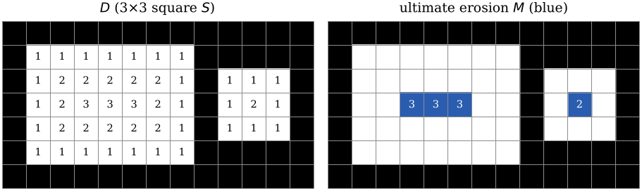
The distance transform by repeated erosion with the \(3\times3\) square (values printed) and the ultimate erosion (blue).
Touching objects form a single connected component, so labelling counts them as one. If the objects are roughly round, each one still has its own peak in \(D\). Growing the peaks back out, without letting two labels merge, splits the clump along its necks.
Input: binary image \(I\) of roughly round objects, some touching. Output: one label per object.
- \(D\leftarrow\) the distance transform of \(I\).
- \(M\leftarrow\) the regional maxima of \(D\); give each component its own label.
- Repeatedly dilate every label by \(S\) inside \(I\), visiting pixels in order of decreasing \(D\).
- A pixel reached by two different labels at once becomes a boundary and is never filled.
- Stop when no label changes.
This is a reconstruction with a no-merge constraint, which is the same thing as a marker-controlled watershed on \(-D\), restricted to \(I\) (see Classical Segmentation). Run the same constrained growth on the background instead of the objects, and it partitions the plane into one zone of influence per object. That partition is the Voronoi tessellation of the objects.

Sixteen discs forming 13 connected components. The Euclidean distance transform \(D\) has 16 maxima \(M\) (enlarged for visibility); growing them back without merging separates all 16 (\(R\), thin cuts). Right: constrained growth into the background gives each object its zone of influence \(V\).
When it fails. The method assumes one distance peak per object. A long or irregular object has a ridge, and noise on its outline breaks that ridge into several local maxima, so the object is over-split. The usual mitigation is to keep only maxima of a minimum depth, but the right depth depends on the shapes in the image, and the nuts-and-bolts images below show how fragile it is.
When to use it vs alternatives. Use it for touching round things: cells, coins, grains, bubbles. For elongated objects, either avoid the touching in the first place (better imaging, better thresholding) or switch to a model that knows the object shape.
the top-hat transform
Everything so far acts after thresholding. Morphology also works before it, on the grey-scale image. Treat the image as a landscape: the set of points \((\mathbf x,z)\) with \(z\le I(\mathbf x)\), called the umbra, is a binary set one dimension up. Apply binary morphology to the umbra and read off the new surface height. For a flat element (zero height on its support) the result is simple.
For a flat, symmetric structuring element \(S\), \[ (I\oplus S)(\mathbf x)=\max_{\mathbf p\in S} I(\mathbf x+\mathbf p),\qquad (I\ominus S)(\mathbf x)=\min_{\mathbf p\in S} I(\mathbf x+\mathbf p), \] and opening and closing are defined from these exactly as in the binary case.
Grey dilation is a local max filter and erosion is a local min filter: max pooling and min pooling with stride 1. Binary morphology is the special case of images that take only the values 0 and 1, where max is OR and min is AND. Grey opening then flattens every bright structure that \(S\) does not fit inside, and keeps larger structures with their edges sharp. No linear filter can do that. A low-pass filter attenuates small blobs but never removes them, and it blurs every edge equally.
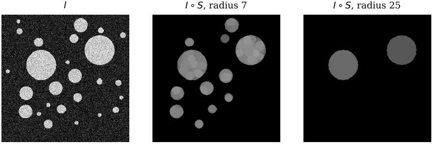
Opening a noisy image of 26 bright discs (radii 4 to 30) with a flat disc. Radius 7 keeps the 12 discs of radius 9 or more; radius 25 keeps only the two of radius 30. The survivors keep sharp edges.
That size selectivity solves a classic thresholding problem: uneven illumination. If the objects are small, a closing (for dark objects) or an opening (for bright objects) with an element larger than the objects erases them and leaves an estimate of the background alone. Subtract that estimate and the objects sit on a flat background.
With a flat \(S\) larger than the objects of interest:
- bright objects on a shaded background: \(O=I-(I\circ S)\ge0\), the white top-hat;
- dark objects on a shaded background: \(O=I-(I\bullet S)\le0\), the negative of the black top-hat \((I\bullet S)-I\).
In both cases \(O\) is zero on the background and non-zero on the objects.
A synthetic image has dark specks on a background that is bright in the middle and darker towards the edges, so no single threshold separates specks from background everywhere. Close it with a disc of radius 10. The dilation (red profile below) rides over the specks along the top of the background, and the erosion (green) brings that estimate back down onto the background, removing the upward shift that dilation alone would leave. Subtracting gives \(O\), which ranges from \(-137.2\) to \(0\). Displayed as \(O+255\) it is flat at 255 with dips at the specks, and one global threshold on it now segments every speck.
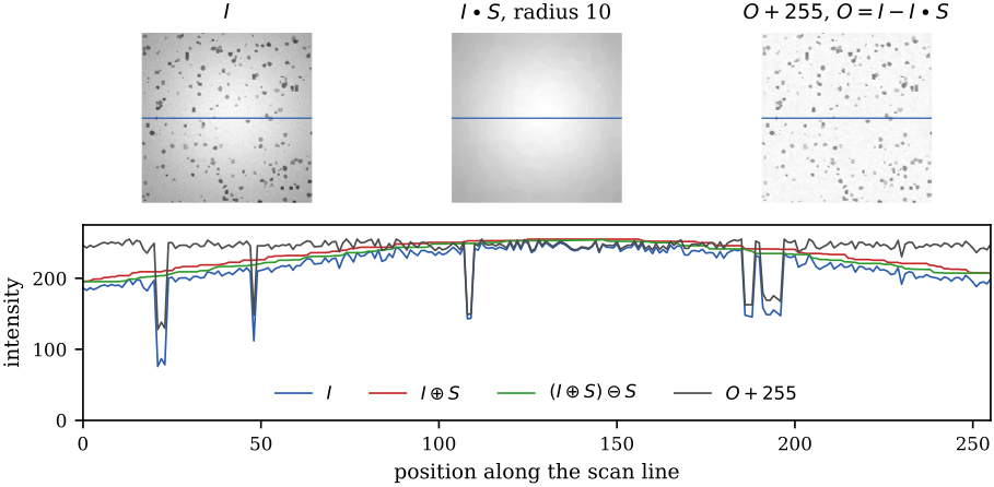
Top-hat filtering. The closing \(I\bullet S\) (disc of radius 10) estimates the background, and \(O=I-I\bullet S\) removes it. Bottom: intensities along the blue scan line.
When it fails. The element has to be larger than every object and smaller than the scale over which the shading changes. An object wider than \(S\) survives the closing, so it is treated as background and subtracted away. Shading that varies over less than the width of \(S\) leaks into \(O\). Clusters of objects closer together than \(S\) also prop up the background estimate between them.
When to use it vs alternatives. Use the top-hat for small objects of known maximum size under slowly varying light. For large objects or unknown sizes, a threshold that varies across the image is safer.
counting nuts and bolts
A manufacturer photographs every batch of fasteners before packing it. Each batch must contain exactly \(N=25\) nuts and \(N=25\) bolts. The software has to count both and print “All good”, or “Add \(X\) nuts” and/or “Add \(Y\) bolts”, or “Remove …”. The constraints: intensity thresholding, binary morphology and simple rules only, fully automatic, with one parameter set for all three test images (dark metal parts on a white background, about \(670\times700\) pixels).
Parameters: \(N=25\), disc \(S_2\) of radius 2, area split \(a^\ast=2500\) pixels.
- Threshold. Compute the Otsu threshold \(t\) and set \(T=\{\mathbf x : I(\mathbf x)\le t\}\). The objects are dark, so the threshold is inverted.
- Close: \(T\leftarrow T\bullet S_2\), sealing cracks and specular glints inside the metal.
- Fill holes by reconstruction, turning each nut ring into a solid hexagon.
- Open: \(T\leftarrow T\circ S_2\), deleting specks in the background.
- Clear the border by reconstruction.
- Label the components with 8-connectivity and measure their areas \(a_k\).
- Classify: nuts are the components with \(a_k<a^\ast\), bolts those with \(a_k\ge a^\ast\).
- Report: test nuts and bolts separately. For each, if the count \(c<N\) report “Add \(N-c\)”, and if \(c>N\) report “Remove \(c-N\)”. If neither test fires, report “All good”.
The order of steps matters. Closing comes before hole filling because a cracked ring has no hole to fill: the crack lets the border flood in. Border clearing and labelling come last because they act on whole components, so they inherit every leftover speck, crack and bridge in the mask. Step 8 needs two independent tests rather than an if-else chain, because a batch can be short of nuts and over on bolts at the same time.
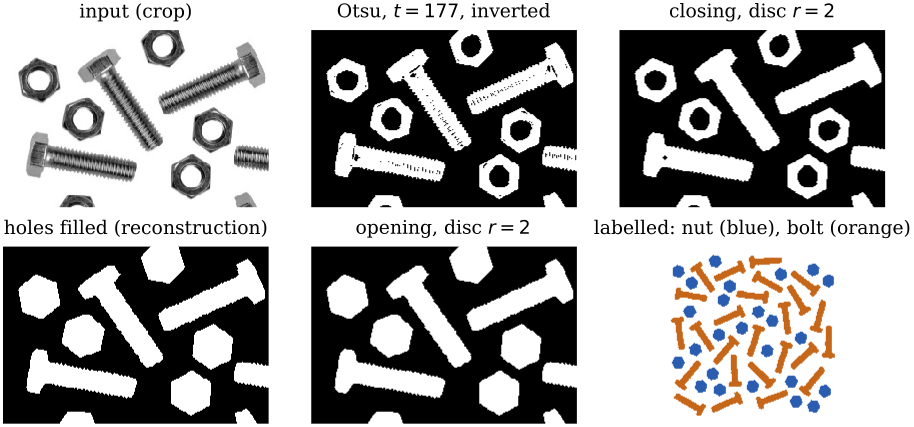
The pipeline on the first image: a crop through threshold, closing, hole filling and opening, then the whole image classified by area (blue: nut, orange: bolt).
the verdicts
| image | Otsu \(t\) | nuts + bolts | output |
|---|---|---|---|
| 1 | 177 | 25 + 25 | All good |
| 2 | 178 | 24 + 25 | Add 1 nut |
| 3 | 178 | 25 + 26 | Remove 1 bolt |
No object touches the border in any of the three images, so step 5 removes nothing. After hole filling the areas form two tight clusters across all 150 objects: nuts 1672 to 1705 pixels, bolts 3297 to 3465. Any split between about 1700 and 3300 classifies every object correctly. Putting \(a^\ast=2500\) in the middle of the gap means a segmentation error of several hundred pixels in either direction would not change a single label.
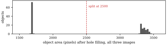
Areas of all 150 objects in the three images after the pipeline: a spike of nuts near 1690 pixels, bolts between 3300 and 3470, and a wide empty gap around the split at 2500.
why the morphology is there
The honest observation is that these three images are clean. Otsu thresholding plus 8-connected labelling alone already gives 50, 49 and 51 components, the right totals. The morphology earns its keep on worse data. To check this, set 1% of the pixels of each image to 0 (pepper) or 255 (salt), with seed 9517:
| image | Otsu, clean | Otsu, 1% noise | after steps 2–5 |
|---|---|---|---|
| 1 | 50 | 3254 | 50 |
| 2 | 49 | 3198 | 49 |
| 3 | 51 | 2934 | 51 |
With noise, thresholding alone produces thousands of components, almost all of them isolated noise pixels. After the clean-up the counts are exactly right again, and the verdicts are unchanged: all good, add 1 nut, remove 1 bolt.
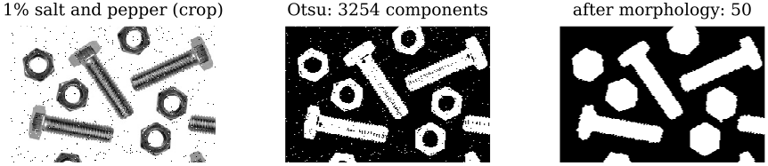
The first image with 1% salt-and-pepper noise (crop). Otsu thresholding alone yields 3254 components; after closing, hole filling, opening and border clearing, 50.
What each step contributes:
- Closing seals salt pixels and thin bright reflections inside the dark metal, which would otherwise notch or crack the objects.
- Hole filling makes a nut’s area independent of its hole and of any noise inside the hole. The classes would still separate without it on these images (ring areas 1215 to 1248 against bolts 3166 to 3207), but the filled area is the more stable feature.
- Opening deletes the pepper pixels in the background. Left in, each one would be counted as a tiny nut.
- Border clearing removes nothing here, but in production it is essential: a bolt cut in half by the frame has roughly the area of a nut.
where it breaks
- Touching parts. Two nuts in contact form one component of about 3400 pixels, which the area rule counts as one bolt. The obvious remedy is distance-transform separation, and the bolts show why it is fragile. The Euclidean distance transform of the first image’s final mask has 184 maxima of depth at least 0.5 pixel and 54 of depth at least 1. Only from depth 2 upwards does it give the correct 50. The long shafts produce spurious peaks, which is exactly the elongated-object failure from earlier.
- Scale. The area split assumes a fixed camera distance. Move the camera and \(a^\ast\) is wrong. A scale-free alternative is a shape measure such as circularity \(4\pi A/P^2\), which is 1 for a disc and smaller for every other shape. On the first image the filled nuts measure 0.677 to 0.856 and the bolts 0.257 to 0.324, so any threshold between 0.33 and 0.67 separates them at any zoom. Hole filling matters here too: with its hole kept, a nut is a ring, and its circularity collapses to about 0.23, because the hole adds a second boundary to \(P\) and removes area from \(A\).
see also
- Classical Segmentation: Otsu thresholding, connected-component labelling and the watershed, the steps on either side of this pipeline
- K-means Clustering: clustering shape features such as circularity, instead of hand-picking a split
- CNN from scratch: max pooling is grey-scale dilation with a stride
- Graph Theory: reconstruction is a flood fill, which is graph search on the pixel adjacency graph
Backlinks (2)
1. Classical Segmentation /wiki/computer-vision/segmentation/
2. Computer Vision /wiki/computer-vision/
I think taking a course in a subject that you are interested in is never particularly a bad thing.
Comments