Motion and Tracking

A single image says what is there. A video also says what moved, and the motion is often the most useful thing in it: it separates a walker from the pavement, tells a car how it is turning, and lets a microscope follow a particle too faint to see in any one frame. This page climbs three rungs. First, where did something change (change detection)? Second, how far and which way did each pixel move (optical flow, with Harris corners explaining where that question even has an answer)? Third, where is the object now, and where will it be next, given a whole history of noisy detections (tracking as Bayesian filtering, solved exactly by the Kalman filter and approximately by the particle filter). 𐃏

Two ideas carry the whole page. Optical flow is a linear-algebra problem: a least-squares solve whose matrix, the structure tensor, is the same matrix Harris uses to find corners. Tracking is a probability problem: a hidden Markov model, filtered by alternating “predict” and “correct”, exactly as on the Markov chains and hidden Markov models page.

change detection

With a still camera and an unchanging background, any pixel whose grey value changes must belong to something that moved. Subtracting frames answers “where?” without estimating any motion at all.

Subtract consecutive frames, $I_t - I_{t-1}$. A uniform object moving a few pixels changes only at its leading edge (object now covers background) and its trailing edge (background uncovered), with opposite signs. Its interior is the same grey in both frames, so it vanishes.

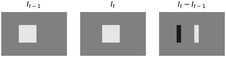
A uniform square (grey 0.9 on 0.5) moves 4 pixels right. The difference is $+0.4$ along the front edge, $-0.4$ along the rear edge and zero inside: of the square’s 256 pixels only 128 change.

So frame differencing localises moving things but returns their edges, not their extent. An object that stops moving disappears entirely.

background subtraction

To recover whole objects, subtract a picture of the empty scene instead of the previous frame, then clean up.

Definition (Algorithm: Change detection by background subtraction)

Input: frame $I_t$, background image $B$, threshold $\tau$, minimum region area, small disk $D$.

Mark $J(x,y) = 1$ wherever $|I_t(x,y) - B(x,y)| > \tau$, else 0. The absolute value matters: objects darker than the background count too.
Label the connected components of $J$.
Delete components smaller than the minimum area; they are noise.
Close $J$ with the disk $D$, fusing fragments of one object.
Report a bounding box per surviving component.

Everything is linear in the number of pixels. The threshold can come from any histogram method (Otsu, triangle) applied to $|I_t - B|$, whose histogram is a tall spike near zero plus a small tail.

Steps 3 and 4 each exist for a reason you can calculate. With Gaussian noise of standard deviation $\sigma_n$ in each image, the difference has standard deviation $\sqrt 2\,\sigma_n$, so the fraction of empty-background pixels that cross the threshold is \[ 2\left(1 - \Phi\!\left(\frac{\tau}{\sqrt 2\,\sigma_n}\right)\right) = 0.008 \quad\text{for } \sigma_n = 0.04,\ \tau = 0.15 . \] That is hundreds of isolated speckles in a modest image, which is why small regions are removed. And an object part that happens to match the background grey falls below $\tau$ and splits the object in two, which is why the closing is there.

Background subtraction on a synthetic still-camera scene ($\sigma_n = 0.04$, $\tau = 0.15$, minimum area 15, disk radius 3). Thresholding leaves 165 regions, area filtering leaves 4, and the closing re-joins the middle walker, whose band has the background’s grey, giving the 3 boxes in (d).

when it fails, and what to use instead

Change detection assumes the background is constant. A moving or shaking camera, swaying trees, shadows and lighting changes all change pixels that belong to no object; an object the same grey as the background is invisible. When the camera moves, everything changes, and the motion itself has to be estimated. That is the next section. Use change detection for fixed surveillance cameras, lab rigs and anything where a clean background frame is available; it is the cheapest detector there is.

brightness constancy

Sparse motion (follow a few distinctive points with template matching) handles large displacements but only at a handful of points. Dense motion, a velocity $\mathbf v = (v_x, v_y)$ at every pixel, is called optical flow. Searching a window for every pixel would be far too slow, so instead the intensity change is linked to the motion analytically.

The assumption is that over a short interval a small patch keeps its content and merely shifts: lighting, distance to the camera and appearance do not change. A moving point keeps its grey value. That is brightness constancy, and it is never exactly true, but it is true enough to compute with.

Theorem (Optical-flow constraint)

Under brightness constancy and for small motion, the flow at each pixel satisfies \[ I_x v_x + I_y v_y = -I_t, \qquad\text{that is}\qquad \nabla I \cdot \mathbf v = -I_t , \] where $I_x, I_y$ are the spatial derivatives and $I_t$ is the temporal derivative of the image.

In practice $I_x, I_y$ come from a derivative kernel (Sobel, say) and $I_t$ from the frame difference with $\Delta t = 1$ frame. Read the equation as: the change you see at a fixed pixel equals the gradient you are looking at, swept past you at velocity $\mathbf v$.

proofs

Proof (Optical-flow constraint)

Brightness constancy says the point at $(x, y)$ at time $t$ reappears at $(x + \Delta x, y + \Delta y)$ at time $t + \Delta t$ with the same value: \[ I(x + \Delta x,\, y + \Delta y,\, t + \Delta t) = I(x, y, t) . \] For small displacements, a first-order Taylor expansion of the left side in all three variables gives \[ I(x + \Delta x,\, y + \Delta y,\, t + \Delta t) \approx I(x, y, t) + I_x\,\Delta x + I_y\,\Delta y + I_t\,\Delta t . \] Equating the two and cancelling $I(x,y,t)$ leaves $I_x\Delta x + I_y\Delta y + I_t\Delta t = 0$. Divide by $\Delta t$ and write $v_x = \Delta x/\Delta t$, $v_y = \Delta y/\Delta t$.

The linearisation is the weak point: it holds only while the displacement is small compared with the scale over which the gradient changes, typically a pixel or two. Larger motions are handled by blurring first or by working coarse-to-fine on an image pyramid, estimating the motion at low resolution and refining it level by level.

the aperture problem

The constraint is one equation in two unknowns. It does not determine $\mathbf v$.

Definition (Aperture problem)

At a single pixel the solutions of $\nabla I \cdot \mathbf v = -I_t$ form a line in the $(v_x, v_y)$ plane, perpendicular to $\nabla I$. Only the component of motion along the gradient is fixed, the normal flow \[ \mathbf v_\perp = \frac{-I_t}{\|\nabla I\|^2}\,\nabla I , \] which is the point of the line closest to the origin. Motion along the edge, perpendicular to the gradient, is invisible.

The name comes from watching through a small window. Slide a long straight edge sideways, diagonally or along itself plus a bit: through a peephole all three look identical, because the edge has no features along its own length.

Example (One pixel’s constraint)

At a pixel $I_x = 2$, $I_y = 1$, $I_t = -4$. The constraint is $2v_x + v_y = 4$, a line through $(2, 0)$, $(1, 2)$ and $(0, 4)$: all three motions explain the pixel equally well. The normal flow is \[ \mathbf v_\perp = \frac{4}{5}(2, 1) = (1.6, 0.8), \] which satisfies $2(1.6) + 0.8 = 4$ and is the shortest solution, of length $0.8\sqrt 5 \approx 1.79$.

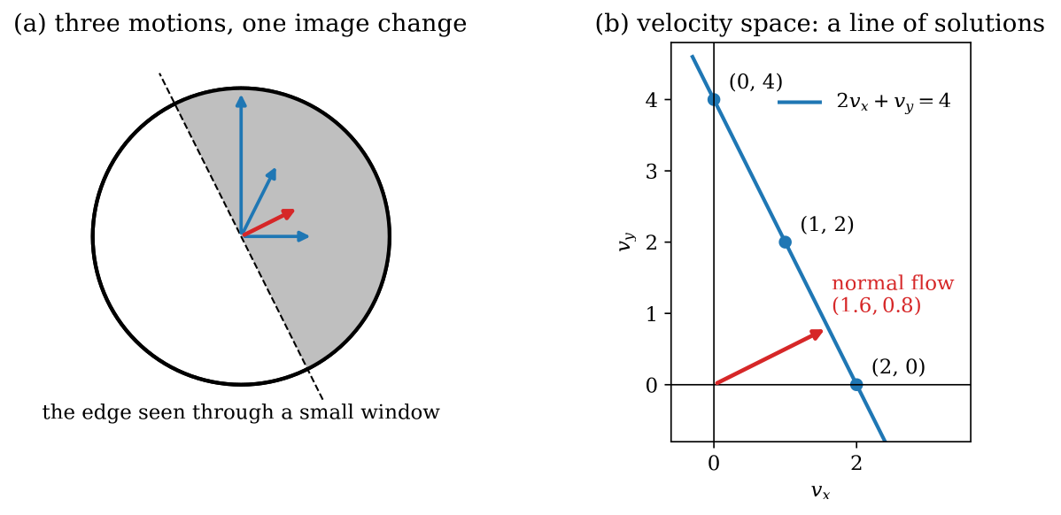
The aperture problem for the example above. (a) Through a small window on a straight edge, the three blue motions and the red normal flow all produce the same image change. (b) In velocity space every solution lies on the constraint line; one pixel pins down only the normal flow, the point nearest the origin.

The cure is another constraint. The simplest is to assume that a small neighbourhood moves as one, so its pixels contribute many equations in the same two unknowns. Whether those equations actually pin $\mathbf v$ down depends on whether the neighbourhood’s gradients point in more than one direction, which is exactly the question a corner detector asks.

corners and the structure tensor

A point can be followed from frame to frame only if its neighbourhood varies in every direction. In a flat patch every shift looks the same; on a straight edge every shift along the edge looks the same. Only at a corner does every shift change what you see.

the quadratic form

Shift a window $W$ by a small $(\Delta x, \Delta y)$ and measure the sum of squared changes, weighted by a window $w$ (box or Gaussian). To first order, \[ E(\Delta x, \Delta y) = \sum_{(x,y)\in W} w(x,y)\,\big(I_x\Delta x + I_y\Delta y\big)^2 = \begin{bmatrix}\Delta x & \Delta y\end{bmatrix} \mathbf M \begin{bmatrix}\Delta x \\ \Delta y\end{bmatrix}, \] with the structure tensor \[ \mathbf M = \sum_{(x,y)\in W} w(x,y) \begin{bmatrix} I_x^2 & I_x I_y \\ I_x I_y & I_y^2 \end{bmatrix}. \] So the eigenvalues $\lambda_1 \ge \lambda_2 \ge 0$ of $\mathbf M$ are the change in the most- and least-changing directions, and they classify the patch at a glance:

patch	$\lambda_1$	$\lambda_2$	can it be tracked?
flat	small	small	no
edge	large	$\approx 0$	only across the edge
corner	large	large	yes

the harris detector

Computing eigenvalues at every pixel is avoidable: the determinant and trace already carry them.

Definition (Algorithm: Harris corner detector)

Input: image $I$, window $w$ (typically Gaussian, $\sigma \approx 1.5$), constant $\alpha \in [0.04, 0.06]$, threshold.

Compute gradients $I_x, I_y$.
At every pixel, form $\mathbf M$ by window-weighting the three products $I_x^2$, $I_xI_y$, $I_y^2$ (three blurs).
Compute the corner response $R = \det\mathbf M - \alpha(\operatorname{tr}\mathbf M)^2$, which in terms of the eigenvalues is $R = \lambda_1\lambda_2 - \alpha(\lambda_1 + \lambda_2)^2$.
Keep local maxima of $R$ above the threshold.

The response sorts the three cases by sign: flat gives $R \approx 0$, an edge gives $R \approx -\alpha\lambda_1^2 < 0$, a corner gives $R > 0$. A cruder cousin, the interest operator, computes the intensity variance along four directions (horizontal, vertical, two diagonals) and keeps a pixel when the minimum is large; Harris is the same test done in all directions at once.

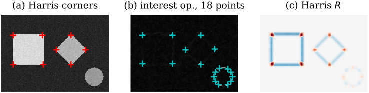
(a) Harris ($\alpha = 0.05$, Gaussian $\sigma = 1.5$) finds exactly the 8 corners of the square and diamond. (b) The four-direction interest operator finds those 8 plus 10 more around the disk, because a curve varies along all four sampled directions. (c) The Harris response: red (positive) at corners, blue (negative) along straight edges, near zero on flat ground.

when it fails, and what to use instead

Harris is rotation-invariant in where it fires but not scale-invariant: a corner seen much larger looks like an edge in a fixed window. If points must be matched across big changes in scale or rotation, use a scale-space detector with a descriptor (see SIFT, Matching and Stitching). Every corner detector fails on repetitive texture such as a brick wall: each corner is found, but each looks like its neighbours, so the matching step that follows picks the wrong one. Use Harris when you need well-localised points to track over small inter-frame motion, which is the classic job feeding Lucas–Kanade.

lucas–kanade optical flow

Lucas and Kanade cure the aperture problem with the neighbourhood assumption: all $n$ pixels $\mathbf p_1, \dots, \mathbf p_n$ of a small window share one velocity $\mathbf v$. Each pixel contributes its own constraint, giving an overdetermined system \[ \underbrace{\begin{bmatrix} I_x(\mathbf p_1) & I_y(\mathbf p_1) \\ \vdots & \vdots \\ I_x(\mathbf p_n) & I_y(\mathbf p_n) \end{bmatrix}}_{\mathbf G} \begin{bmatrix} v_x \\ v_y \end{bmatrix} = \underbrace{\begin{bmatrix} -I_t(\mathbf p_1) \\ \vdots \\ -I_t(\mathbf p_n) \end{bmatrix}}_{\mathbf b}. \] Noise makes it inconsistent, so take the least-squares solution from the normal equations, $\mathbf G^\top\mathbf G\,\mathbf v = \mathbf G^\top\mathbf b$: \[ \mathbf v = (\mathbf G^\top\mathbf G)^{-1}\mathbf G^\top\mathbf b, \qquad \mathbf G^\top\mathbf G = \begin{bmatrix} \sum I_x^2 & \sum I_xI_y \\ \sum I_xI_y & \sum I_y^2 \end{bmatrix}, \qquad \mathbf G^\top\mathbf b = -\begin{bmatrix} \sum I_xI_t \\ \sum I_yI_t \end{bmatrix}. \]

Look at that matrix. $\mathbf G^\top\mathbf G$ is the structure tensor $\mathbf M$ with a box window. So Lucas–Kanade is reliable exactly where Harris would report a corner, both eigenvalues large. On an edge $\lambda_2 \approx 0$, the matrix is nearly singular, and only the normal flow comes out: the aperture problem, reappearing as an ill-conditioned $2\times 2$ solve. In a flat region nothing comes out at all. The corner detector and the flow estimator are one idea seen from two sides.

Definition (Algorithm: Lucas–Kanade optical flow)

Input: frames $I_t, I_{t+1}$, window size, eigenvalue threshold $\lambda_{\min}$.

Compute $I_x, I_y$ with a derivative kernel and $I_t \approx I_{t+1} - I_t$, at every pixel.
For each pixel, sum $I_x^2$, $I_xI_y$, $I_y^2$, $I_xI_t$, $I_yI_t$ over its window (box filters make this $O(1)$ per pixel).
If the smaller eigenvalue of $\mathbf G^\top\mathbf G$ is at least $\lambda_{\min}$, solve the $2\times 2$ system for $\mathbf v$.
Otherwise mark the pixel undetermined (an edge or a flat patch).

The window must be big enough to contain gradients in two directions and small enough that the motion inside it is uniform.

Example (Lucas–Kanade by hand)

A five-pixel window has

pixel	$I_x$	$I_y$	$I_t$
$\mathbf p_1$	1	0	$-1$
$\mathbf p_2$	0	1	0.5
$\mathbf p_3$	1	1	$-0.5$
$\mathbf p_4$	2	$-1$	$-2.5$
$\mathbf p_5$	1	2	0

The sums are $\sum I_x^2 = 7$, $\sum I_y^2 = 7$, $\sum I_xI_y = 1$, and with $\mathbf b = -I_t = (1, -0.5, 0.5, 2.5, 0)$, $\mathbf G^\top\mathbf b = (6.5, -2.5)$. Then \[ \mathbf v = \frac{1}{48}\begin{bmatrix} 7 & -1 \\ -1 & 7 \end{bmatrix}\begin{bmatrix} 6.5 \\ -2.5 \end{bmatrix} = \frac{1}{48}\begin{bmatrix} 48 \\ -24 \end{bmatrix} = \begin{bmatrix} 1 \\ -0.5 \end{bmatrix}. \] Check $\mathbf p_4$: $2(1) + (-1)(-0.5) = 2.5 = -I_t$. All five residuals vanish: one pixel right, half a pixel up (image $y$ points down). The eigenvalues are $7 \pm 1$, both large, and the Harris response is $R = 48 - 0.05 \cdot 14^2 = 38.2 > 0$: a corner, so a trustworthy estimate.

Now replace the gradients by three parallel ones, $(1, 2)$, $(2, 4)$, $(-1, -2)$. Then $\mathbf G^\top\mathbf G = \begin{bmatrix} 6 & 12 \\ 12 & 24 \end{bmatrix}$ has determinant 0, no inverse, and $R = 0 - 0.05 \cdot 30^2 = -45$: an edge, and the aperture problem.

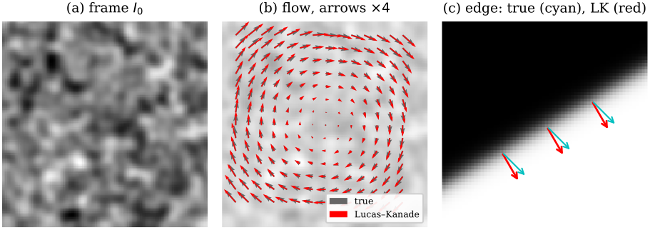
Lucas–Kanade with a $9\times 9$ window. (a) A textured frame. (b) The second frame is the first rotated by 2 degrees; the estimated flow (red) tracks the true flow (grey) with mean error 0.16 pixels for speeds up to 2.7 pixels (arrows drawn 4 times longer). (c) A straight edge moved by $(1, 1)$: the estimate (red) is the normal flow, perpendicular to the edge, not the true motion (cyan). The smaller eigenvalue there is $10^{-5}$ of the larger.

when it fails, and what to use instead

Lucas–Kanade inherits every assumption on the way here. Large displacements break the Taylor step: use a pyramid (coarse-to-fine) or template matching, which searches a region and tolerates any shift inside it but costs a search per point. Lighting changes break brightness constancy. Motion boundaries break the “one window, one velocity” assumption, blurring the flow across object edges. Edges and flat regions give no answer, by design. So: Lucas–Kanade run at corners is the classic sparse tracker (the KLT tracker, which picks points by the smaller eigenvalue of $\mathbf M$ rather than by $R$); dense Lucas–Kanade is fast but holey; and template matching is the choice when motion is large, points are few and appearance is stable.

tracking as bayesian filtering

Flow relates two frames. Tracking follows an object through the whole sequence, and that changes the problem. Detections are noisy, sometimes missing, sometimes confused with clutter; the object might be invisible for a while. A human watching a particle at a signal-to-noise ratio of 1.5 can still follow it, because the eye integrates over time and expects smooth motion. A tracker has to do the same thing explicitly: keep a probability distribution over the object’s state and update it frame by frame.

the model

The state $\mathbf x_i$ at step $i$ holds whatever we care about: position, velocity, perhaps size or appearance. The measurement $\mathbf y_i$ is what the image gives us, such as a detected position. Write $\mathbf y_{0:i}$ for all measurements up to step $i$. Two assumptions make the problem tractable:

the state is Markov: $p(\mathbf x_i \mid \mathbf x_{0:i-1}) = p(\mathbf x_i \mid \mathbf x_{i-1})$;
each measurement depends only on the current state: $p(\mathbf y_i \mid \mathbf x_{0:i}, \mathbf y_{0:i-1}) = p(\mathbf y_i \mid \mathbf x_i)$.

Together they say tracking is inference on a hidden Markov model: the states are hidden, the measurements are seen. Two models must be designed for each application: the dynamics model $p(\mathbf x_i \mid \mathbf x_{i-1})$ (say, constant velocity plus random acceleration) and the measurement model $p(\mathbf y_i \mid \mathbf x_i)$ (how likely this image evidence is, if the object is there).

the predict–update recursion

Theorem (Bayesian tracking recursion)

Under the hidden-Markov assumptions the filtering density $p(\mathbf x_i \mid \mathbf y_{0:i})$ is computed recursively by \[ \text{predict:}\quad p(\mathbf x_i \mid \mathbf y_{0:i-1}) = \int p(\mathbf x_i \mid \mathbf x_{i-1})\, p(\mathbf x_{i-1} \mid \mathbf y_{0:i-1})\, d\mathbf x_{i-1}, \] \[ \text{correct:}\quad p(\mathbf x_i \mid \mathbf y_{0:i}) \propto p(\mathbf y_i \mid \mathbf x_i)\, p(\mathbf x_i \mid \mathbf y_{0:i-1}). \] Prediction pushes yesterday’s belief through the dynamics; correction reweights it by today’s evidence (Bayes’ rule). The output feeds the next prediction.

With several objects, or clutter, a third step sits between the two: association, deciding which detection belongs to which track, usually the one most probable under the prediction.

The posterior is a whole distribution, and a single answer has to be read off it. The two standard choices are the posterior mean (expected a posteriori, EAP) and the posterior mode (maximum a posteriori, MAP). For a Gaussian they coincide. For a multimodal posterior the mean can land in a valley where the object almost certainly is not.

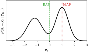
EAP versus MAP on the bimodal posterior $0.45\,\mathcal N(-1.2, 0.6^2) + 0.55\,\mathcal N(1, 0.5^2)$. The MAP sits on the higher peak at 1.00; the EAP is 0.01, in the trough between the two hypotheses.

Example (A Bayes filter on five cells)

An object lives on cells 1–5. Yesterday’s posterior is $(0.1, 0.6, 0.3, 0, 0)$. Dynamics: move one cell right with probability 0.7, stay with 0.3. Today’s detector gives likelihood $(0.1, 0.1, 0.2, 0.8, 0.2)$.

Predict (the integral becomes a sum): cell 2 receives $0.7 \cdot 0.1 + 0.3 \cdot 0.6 = 0.25$, cell 3 receives $0.7 \cdot 0.6 + 0.3 \cdot 0.3 = 0.51$, and so on. Correct: multiply by the likelihood and normalise (the unnormalised sum is 0.298).

cell	predicted	likelihood	posterior
1	0.03	0.1	0.010
2	0.25	0.1	0.084
3	0.51	0.2	0.342
4	0.21	0.8	0.564
5	0	0.2	0

The prediction favoured cell 3; the detector pulled the posterior to cell 4 (MAP). The EAP is 3.46, which is not a cell at all.

On a grid the integral is a sum and everything is exact. In a continuous state space the integral is generally intractable, and the two filters below are the two ways out: make everything Gaussian so it can be done in closed form, or replace the density by samples.

proofs

Proof (Bayesian tracking recursion)

Prediction. Marginalise over the previous state, factor with the product rule, then drop the old measurements by the Markov property (given $\mathbf x_{i-1}$, they say nothing more about $\mathbf x_i$):

\begin{align} p(\mathbf x_i \mid \mathbf y_{0:i-1}) &= \int p(\mathbf x_i, \mathbf x_{i-1} \mid \mathbf y_{0:i-1})\, d\mathbf x_{i-1} \\ &= \int p(\mathbf x_i \mid \mathbf x_{i-1}, \mathbf y_{0:i-1})\, p(\mathbf x_{i-1} \mid \mathbf y_{0:i-1})\, d\mathbf x_{i-1} \\ &= \int p(\mathbf x_i \mid \mathbf x_{i-1})\, p(\mathbf x_{i-1} \mid \mathbf y_{0:i-1})\, d\mathbf x_{i-1} . \end{align}

Correction. Split off the newest measurement and use the measurement assumption:

\begin{align} p(\mathbf x_i \mid \mathbf y_{0:i}) &= \frac{p(\mathbf y_i \mid \mathbf x_i, \mathbf y_{0:i-1})\, p(\mathbf x_i \mid \mathbf y_{0:i-1})\, p(\mathbf y_{0:i-1})}{p(\mathbf y_{0:i})} \\ &= p(\mathbf y_i \mid \mathbf x_i)\, p(\mathbf x_i \mid \mathbf y_{0:i-1}) \cdot \frac{p(\mathbf y_{0:i-1})}{p(\mathbf y_{0:i})} . \end{align}

The last factor does not involve $\mathbf x_i$; it is recovered by normalising.

the kalman filter

If the dynamics and measurements are linear with additive Gaussian noise, and the initial belief is Gaussian, then every density in the recursion stays Gaussian: a linear map of a Gaussian plus independent Gaussian noise is Gaussian, and a Gaussian prior times a Gaussian likelihood is Gaussian. A Gaussian is just a mean and a covariance, so the filter propagates two quantities instead of a whole function.

Definition (Linear–Gaussian state-space model)

\[ \mathbf x_i = \mathbf A\,\mathbf x_{i-1} + \mathbf q_{i-1},\quad \mathbf q \sim \mathcal N(\mathbf 0, \mathbf Q); \qquad \mathbf y_i = \mathbf H\,\mathbf x_i + \mathbf r_i,\quad \mathbf r \sim \mathcal N(\mathbf 0, \mathbf R), \] with independent noises. $\mathbf A$ is the dynamics matrix, $\mathbf H$ the measurement matrix, $\mathbf Q$ and $\mathbf R$ the process- and measurement-noise covariances.

One cycle moves the density in three ways: the dynamics drift it, the process noise diffuses (widens) it, and the measurement sharpens it. In the Gaussian case it stays one bump throughout; in general it need not.

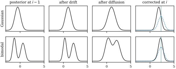
One predict–correct cycle: drift by 1.5, diffusion by $\mathcal N(0, 0.5^2)$, then correction by a measurement at 2.3 (likelihood dashed). Top: a Gaussian stays Gaussian, ending at mean 1.82, which is the Kalman case. Bottom: a two-peaked belief stays two-peaked until the measurement kills one peak, which no Kalman filter can represent.

Definition (Algorithm: Kalman filter)

Input: $\mathbf A, \mathbf H, \mathbf Q, \mathbf R$; initial estimate $\hat{\mathbf x}_0$ with covariance $\mathbf P_0$. For each new measurement $\mathbf y_i$:

Predict the state: $\hat{\mathbf x}_i^- = \mathbf A\,\hat{\mathbf x}_{i-1}$.
Predict the covariance: $\mathbf P_i^- = \mathbf A\,\mathbf P_{i-1}\mathbf A^\top + \mathbf Q$.
Gain: $\mathbf K_i = \mathbf P_i^-\mathbf H^\top(\mathbf H\mathbf P_i^-\mathbf H^\top + \mathbf R)^{-1}$.
Correct the state with the innovation: $\hat{\mathbf x}_i = \hat{\mathbf x}_i^- + \mathbf K_i(\mathbf y_i - \mathbf H\hat{\mathbf x}_i^-)$.
Correct the covariance: $\mathbf P_i = (\mathbf I - \mathbf K_i\mathbf H)\,\mathbf P_i^-$.

Each step costs a few small matrix products and one $m\times m$ inverse ($m$ = measurement dimension), independent of image size.

The innovation $\mathbf y_i - \mathbf H\hat{\mathbf x}_i^-$ is the part of the measurement the prediction did not expect, and the gain decides how much of it to believe. In one dimension with $A = H = 1$ the update is a weighted average, \[ \hat x_i = (1 - K_i)\,\hat x_i^- + K_i\,y_i, \qquad K_i = \frac{P_i^-}{P_i^- + R}, \qquad \frac{1}{P_i} = \frac{1}{P_i^-} + \frac{1}{R} . \] A precise sensor ($R \to 0$) sends $K_i \to 1$ and the filter follows the measurements; a noisy one ($R \to \infty$) sends $K_i \to 0$ and the filter trusts its prediction. Precisions add, so the corrected belief is tighter than either the prediction or the measurement alone. Tuning a Kalman filter is mostly choosing the ratio of $\mathbf Q$ to $\mathbf R$.

a constant-velocity target

To follow a point in the image plane, take the state $\mathbf x = (x, y, v_x, v_y)^\top$, one frame per step, and measure position only: \[ \mathbf A = \begin{bmatrix} 1 & 0 & 1 & 0 \\ 0 & 1 & 0 & 1 \\ 0 & 0 & 1 & 0 \\ 0 & 0 & 0 & 1 \end{bmatrix}, \qquad \mathbf H = \begin{bmatrix} 1 & 0 & 0 & 0 \\ 0 & 1 & 0 & 0 \end{bmatrix}. \] $\mathbf A$ adds velocity to position and keeps velocity; random accelerations enter through $\mathbf Q$. This is the “location and velocity change smoothly” assumption written as a matrix.

Example (One Kalman step on the constant-velocity model)

The $x$ coordinate decouples, so take its block: state $(x, v_x)$, estimate $(10, 2)$, $\mathbf P = \operatorname{diag}(1, 0.5)$, $\mathbf Q = \mathbf 0$, $R = 1$, and a measured position $y = 13$.

Predict: $\hat{\mathbf x}^- = (12, 2)$, and \[ \mathbf P^- = \begin{bmatrix} 1 & 1 \\ 0 & 1 \end{bmatrix}\begin{bmatrix} 1 & 0 \\ 0 & 0.5 \end{bmatrix}\begin{bmatrix} 1 & 0 \\ 1 & 1 \end{bmatrix} = \begin{bmatrix} 1.5 & 0.5 \\ 0.5 & 0.5 \end{bmatrix}. \] Position uncertainty grows, and position and velocity become correlated.
Gain: $\mathbf H\mathbf P^-\mathbf H^\top + R = 2.5$, so $\mathbf K = (1.5, 0.5)/2.5 = (0.6, 0.2)$.
Correct: the innovation is $13 - 12 = 1$, so $\hat{\mathbf x} = (12.6, 2.2)$, and \[ \mathbf P = \begin{bmatrix} 0.6 & 0.2 \\ 0.2 & 0.4 \end{bmatrix}. \]

Only position was measured, yet the velocity estimate rose from 2 to 2.2. The correlation the prediction created carries the surprise into the unmeasured component; that is how a Kalman filter learns velocities it never observes.

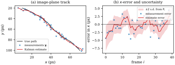
$The constant-velocity Kalman filter over 40 frames with 2-pixel measurement noise and white-acceleration process noise ($q = 0.05$). (a) True path, measurements and estimate. (b) Error in $x$: the estimate’s RMS error is 1.86 pixels against 2.87 for the raw measurements, inside a $\pm 2$ s.d. band from $\mathbf P_i$ that narrows as the gain falls from 0.78 to 0.38.$

The constant-velocity Kalman filter over 40 frames with 2-pixel measurement noise and white-acceleration process noise ($q = 0.05$). (a) True path, measurements and estimate. (b) Error in $x$: the estimate’s RMS error is 1.86 pixels against 2.87 for the raw measurements, inside a $\pm 2$ s.d. band from $\mathbf P_i$ that narrows as the gain falls from 0.78 to 0.38.

proofs

Proof (Kalman filter)

Prediction. If $\mathbf x_{i-1} \mid \mathbf y_{0:i-1} \sim \mathcal N(\hat{\mathbf x}_{i-1}, \mathbf P_{i-1})$, then $\mathbf A\mathbf x_{i-1} + \mathbf q_{i-1}$ has mean $\mathbf A\hat{\mathbf x}_{i-1}$ (the noise has mean zero) and covariance $\mathbf A\mathbf P_{i-1}\mathbf A^\top + \mathbf Q$ (a linear map $\mathbf A$ sends a covariance $\mathbf P$ to $\mathbf A\mathbf P\mathbf A^\top$, and independent terms add covariances).

Correction. For jointly Gaussian $\mathbf u, \mathbf w$, \[ \mathbf u \mid \mathbf w \sim \mathcal N\big(\boldsymbol\mu_u + \Sigma_{uw}\Sigma_{ww}^{-1}(\mathbf w - \boldsymbol\mu_w),\ \Sigma_{uu} - \Sigma_{uw}\Sigma_{ww}^{-1}\Sigma_{wu}\big). \] Take $\mathbf u = \mathbf x_i$ and $\mathbf w = \mathbf y_i = \mathbf H\mathbf x_i + \mathbf r_i$, both conditioned on $\mathbf y_{0:i-1}$. Then $\boldsymbol\mu_u = \hat{\mathbf x}_i^-$, $\Sigma_{uu} = \mathbf P_i^-$, $\boldsymbol\mu_w = \mathbf H\hat{\mathbf x}_i^-$, $\Sigma_{ww} = \mathbf H\mathbf P_i^-\mathbf H^\top + \mathbf R$, and, because $\mathbf r_i$ is independent of $\mathbf x_i$, $\Sigma_{uw} = \mathbf P_i^-\mathbf H^\top$. So $\Sigma_{uw}\Sigma_{ww}^{-1} = \mathbf K_i$, the conditional mean is $\hat{\mathbf x}_i^- + \mathbf K_i(\mathbf y_i - \mathbf H\hat{\mathbf x}_i^-)$, and the conditional covariance is $\mathbf P_i^- - \mathbf K_i\mathbf H\mathbf P_i^- = (\mathbf I - \mathbf K_i\mathbf H)\mathbf P_i^-$.

when it fails

The Kalman filter is optimal for linear–Gaussian models and nothing else. Its belief is always one Gaussian, so it cannot hold two hypotheses at once: the object went behind the left occluder or the right one; the target is one of these three similar blobs. Faced with that, it averages them and sits in the gap, which is the EAP-in-the-valley picture above. Nonlinear dynamics or measurements break the closed form; the extended and unscented Kalman filters patch this by linearising or by pushing a few sigma points through the nonlinearity, and work while the belief remains roughly one bump. When it does not, use a particle filter.

the particle filter

When the models are nonlinear or the noise non-Gaussian, the belief can take any shape, including several peaks. The particle filter stops trying to parameterise it and represents it by samples.

Definition (Particle representation)

The filtering density is represented by $N_p$ samples (particles) $\mathbf s_i^{(n)}$ with weights $\pi_i^{(n)} \ge 0$ summing to 1. High-density regions hold many particles or heavy ones. Any estimate is a weighted sum; the EAP is \[ \hat{\mathbf x}_i = \sum_{n=1}^{N_p} \pi_i^{(n)}\,\mathbf s_i^{(n)} , \] and the heaviest particle approximates the MAP.

Definition (Algorithm: Particle filter, CONDENSATION)

Input: the previous weighted set, a dynamics model you can sample, a measurement model you can evaluate, and the new measurement $\mathbf y_i$. For each $n = 1, \dots, N_p$:

Select: draw an old particle with probability equal to its weight (sample $r \sim U[0,1]$ and binary-search the cumulative weights).
Predict: move the copy through the dynamics, $\mathbf s_i^{(n)} \sim p(\mathbf x_i \mid \mathbf x_{i-1} = \text{copy})$.
Measure: weight it by the likelihood, $\pi_i^{(n)} = p(\mathbf y_i \mid \mathbf x_i = \mathbf s_i^{(n)})$.

Finally normalise the weights and report the weighted mean. Cost: $O(N_p\log N_p)$ for selection plus $N_p$ likelihood evaluations, which dominate because each compares a hypothesis with the image.

Each step is one piece of the recursion. Selection (resampling) turns the weighted set into an unweighted one with the same distribution: heavy particles are duplicated, light ones die. Prediction does the integral by sampling: the random part of the dynamics spreads the duplicates apart, and the cloud now samples $p(\mathbf x_i \mid \mathbf y_{0:i-1})$. Measurement multiplies by the likelihood, exactly the correction step, and normalising replaces the proportionality constant. Nowhere does it need linearity, Gaussian noise or a single peak. The method is also known as sequential Monte Carlo or the bootstrap filter; CONDENSATION is Isard and Blake’s name for it in vision.

Example (One particle-filter step by hand)

Four particles at $s = (2.0, 3.5, 5.0, 7.0)$ with weights $(0.1, 0.4, 0.2, 0.3)$; dynamics $x_i = x_{i-1} + 1 + q$; likelihood $p(y \mid x) \propto e^{-(y - x)^2/2}$; measurement $y = 6$.

Cumulative weights $(0.1, 0.5, 0.7, 1.0)$. Draws $r = 0.62, 0.05, 0.91, 0.33$ select particles 3, 1, 4, 2: $(5.0, 2.0, 7.0, 3.5)$.
Predict with noise $q = (0.2, -0.1, 0, 0.3)$: $(6.2, 2.9, 8.0, 4.8)$.
Likelihoods $(0.980, 0.008, 0.135, 0.487)$, normalised to $(0.609, 0.005, 0.084, 0.302)$.
EAP, the weighted mean of the predicted positions: $0.609(6.2) + 0.005(2.9)$ plus $0.084(8.0) + 0.302(4.8)$, which is $5.91$.

The particle that landed near the measurement carries most of the weight; the one at 2.9 is effectively dead and will vanish at the next selection.

tracking in clutter

The showcase is a target lost among false detections. Each frame below has the true detection plus three random clutter points, and for six frames the target is occluded, so only clutter arrives. The measurement model is a mixture (a detection is either the target or clutter), so the posterior is genuinely multimodal, and a Kalman filter would be dragged towards whichever false alarm sat nearest its single bump.

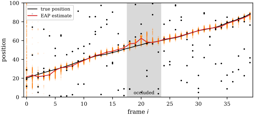
A particle filter ($N_p = 500$) tracking a 1D position. Black dots are detections, three of them clutter in every frame and all of them clutter in the grey occlusion. Orange: particles, area proportional to weight. Starting from particles spread over the whole range, it locks on within five frames (mean error 2.42 over frames 0–4, then 1.08 for the rest), drifts at most 6.95 during the occlusion as the cloud widens, and recovers to a mean error of 0.63 over the last ten frames.

Watch the occlusion: with no real evidence the cloud spreads under the dynamics, the honest response to not knowing. When the target reappears the particles nearest it win the weights and the cloud snaps back. The same machinery tracks spline outlines of a head through cluttered edges, or a pedestrian’s bounding box $(x, y, w, h)$, which is where CONDENSATION made its name.

when it fails

Particles must cover the region where the posterior has mass. In a high-dimensional state the volume grows exponentially and no affordable $N_p$ covers it. If the likelihood is very sharp, or the target jumps somewhere the dynamics did not predict, every particle gets a tiny weight, one particle takes everything after resampling, and the cloud collapses (degeneracy). The answer is random: two runs differ, and small $N_p$ gives noisy estimates. Remedies are more particles, broader dynamics noise, or better proposals that look at the measurement before moving the particles.

which to use

All three filters run the same recursion; they differ in how they store the belief.

	Kalman	particle
models	linear, Gaussian noise	any you can sample and evaluate
belief	one Gaussian	weighted samples, any shape
cost	tiny, deterministic	$N_p$ likelihoods, random
fails when	nonlinear or multimodal	state high-dimensional

On a small discrete state space (a grid of cells, a few labels), run the exact Bayes filter: it is just sums.
For one target with smooth motion and a reliable detector, use a Kalman filter with a constant-velocity model. It is cheap, its covariance tells you how far to search for the next detection, and it is the default in practice.
For mildly nonlinear models with a still-unimodal belief, use the extended or unscented Kalman filter.
For clutter, occlusion, look-alike distractors or strongly nonlinear measurements (contours, appearance models), use a particle filter, provided the state has only a handful of dimensions.

And for the motion estimates that feed them: change detection when the camera is still, Harris plus Lucas–Kanade for small motion at well-textured points, and template matching when motion is large and the points are few.

pixel	\(I_x\)	\(I_y\)	\(I_t\)
\(\mathbf p_1\)	1	0	\(-1\)
\(\mathbf p_2\)	0	1	0.5
\(\mathbf p_3\)	1	1	\(-0.5\)
\(\mathbf p_4\)	2	\(-1\)	\(-2.5\)
\(\mathbf p_5\)	1	2	0

Motion and Tracking

change detection