Classical Segmentation
Counting cells, measuring a tumour or picking nuts off a conveyor all need one step between “an image” and “numbers about what is in it”: deciding which pixels belong together. That step is segmentation: give every pixel a region label so that pixels with the same label form one meaningful segment. 𐃏
Two flavours matter. A semantic segmentation says which pixels are nuts; an instance segmentation says which pixels are nut number 7. Classical pipelines usually get the first from a per-pixel rule and the second from grouping connected pixels. Segmentation would be easy if regions were uniform inside, clearly different from their neighbours, free of holes, and had smooth boundaries. Real images break all four, and each method below is best read as a bet on which of those assumptions still holds. There is no universal winner, so this page is a toolbox, closed by the scores used to compare its tools.
thresholding and Otsu’s method
The simplest segmentation looks at each pixel alone: with threshold \(\tau\), label a pixel object if \(I(x,y) \ge \tau\) and background otherwise. It works exactly when the histogram has two well-separated humps and \(\tau\) sits in the valley between them. The whole question is how to pick \(\tau\) without a human squinting at a slider.
the idea: two tight classes
Otsu’s answer: choose the split that makes each class as tight as possible around its own mean. For a candidate \(t\), with normalised histogram \(p( r)\) over grey levels \(0, \dots, L-1\), let \(P_0, P_1\) be the fractions of pixels below and at-or-above \(t\), \(\mu_0, \mu_1\) the class means and \(\sigma_0^2, \sigma_1^2\) the class variances.
For every threshold \(t\) with both classes non-empty, the total variance splits as \[ \sigma_T^2 = \underbrace{P_0\sigma_0^2 + P_1\sigma_1^2}_{\sigma_W^2(t),\ \text{within-class}} + \underbrace{P_0 P_1 (\mu_0 - \mu_1)^2}_{\sigma_B^2(t),\ \text{between-class}} . \] Since \(\sigma_T^2\) does not depend on \(t\), minimising the within-class variance and maximising the between-class variance pick the same threshold.
The second form is the one to compute. \(\sigma_W^2\) needs two fresh sums of squares for every \(t\), which is \(O(L^2)\) in all. \(\sigma_B^2\) needs only \(P_0(t)\) and the partial first moment \(m(t) = \sum_{r<t} r\,p( r)\), and both are running sums that gain one term as \(t\) increases.
- Build the normalised histogram \(p( r)\) and the overall mean \(\mu = \sum_r r\,p( r)\).
- For \(t = 1, \dots, L-1\), update \(P_0 \leftarrow P_0 + p(t-1)\) and \(m \leftarrow m + (t-1)\,p(t-1)\).
- If \(0 < P_0 < 1\), set \(\mu_0 = m/P_0\), \(\mu_1 = (\mu - m)/(1 - P_0)\) and \(\sigma_B^2(t) = P_0(1-P_0)(\mu_0 - \mu_1)^2\).
- Return the \(t^*\) with the largest \(\sigma_B^2\): class 0 is \(r < t^*\), class 1 is \(r \ge t^*\).
Cost: one pass over the pixels for the histogram, then \(O(L)\). No parameters at all.
Sixteen pixels, eight grey levels, histogram \(h = (1,3,4,2,1,1,3,1)\), so \(\mu = 51/16 = 3.1875\).
| \(t\) | \(P_0\) | \(\sigma_B^2\) | \(\sigma_W^2\) |
|---|---|---|---|
| 1 | 0.0625 | 0.677 | 3.850 |
| 2 | 0.25 | 1.980 | 2.547 |
| 3 | 0.5 | 3.285 | 1.242 |
| 4 | 0.625 | 3.688 | 0.840 |
| 5 | 0.6875 | 3.596 | 0.932 |
| 6 | 0.75 | 3.126 | 1.401 |
| 7 | 0.9375 | 0.969 | 3.558 |
At \(t = 4\): class 0 holds levels 0–3 with \(\mu_0 = (0 + 3 + 8 + 6)/10 = 1.7\), class 1 holds 4–7 with \(\mu_1 = 34/6 = 5.667\), so \[ \sigma_B^2 = \tfrac{10}{16} \cdot \tfrac{6}{16} \cdot 3.967^2 = 3.688 , \] the maximum. Every row satisfies \(\sigma_W^2 + \sigma_B^2 = 4.527 = \sigma_T^2\), so the minimum of one column sits exactly where the other peaks.
On a real photograph the two curves are mirror images about the constant total variance:
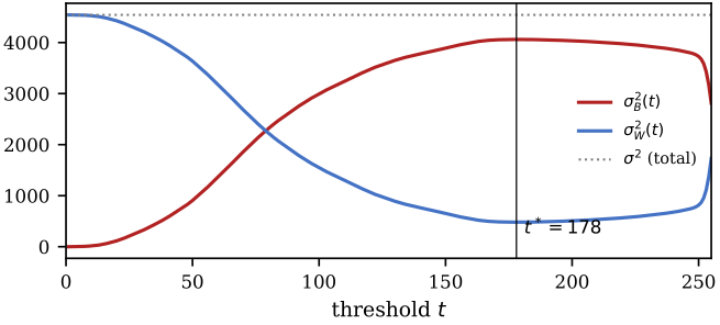
Otsu’s criterion on the first Lab 4 nuts-and-bolts image. The between-class variance (red) and within-class variance (blue) sum to the total at every threshold, so the peak of one is the trough of the other, at \(t^* = 178\).
when it works and when it fails
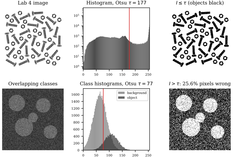
Top: dark metal parts on a bright background give two clean humps, and Otsu’s split (objects are \(I \le 177\), the same split as \(t^* = 178\) above) is essentially perfect. Bottom: five synthetic discs whose intensities overlap the background’s (means 0.42 and 0.25, noise 0.10). Otsu still lands in the right place, but 25.6% of pixels are wrong.
The bottom row is the fundamental limit: when the class histograms overlap, every global \(\tau\) misclassifies the overlap, and moving \(\tau\) only trades false objects for holes. The fix is not a cleverer threshold but more information per pixel: smooth first so neighbours vote, or use region and shape methods below.
The other failure is a skewed histogram. Otsu assumes two classes of comparable size; with a few small bright spots on a large, unevenly lit background it cheerfully splits the background in two.
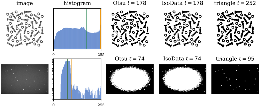
Otsu (and its iterative cousin IsoData) against the triangle method. On the bimodal nuts and bolts, Otsu wins and the triangle method hugs the saturated background peak. On 24 bright spots over a dark gradient, Otsu cuts the background into a blob; the triangle method finds exactly the 24 spots.
When to use it. Otsu is the default for a bimodal histogram with classes of similar size: parameter-free and instant. Use the triangle method for a single dominant peak with a long tail (few small objects), remove uneven illumination first (a top-hat, see Morphology) or threshold tile by tile, and when classes genuinely overlap, stop thresholding raw pixels.
proofs
Split \(\sigma_T^2 = \sum_r (r-\mu)^2 p( r)\) at \(t\), and inside each class write \(r - \mu = (r - \mu_k) + (\mu_k - \mu)\). The cross terms vanish because \(\sum_{r<t}(r - \mu_0)p( r) = 0\) (and likewise for class 1), leaving \[ \sigma_T^2 = P_0\sigma_0^2 + P_1\sigma_1^2 + P_0(\mu_0-\mu)^2 + P_1(\mu_1-\mu)^2 . \] The overall mean is \(\mu = P_0\mu_0 + P_1\mu_1\) with \(P_0 + P_1 = 1\), so \(\mu_0 - \mu = P_1(\mu_0 - \mu_1)\) and \(\mu_1 - \mu = P_0(\mu_1 - \mu_0)\). The last two terms become \[ P_0P_1^2(\mu_0-\mu_1)^2 + P_1P_0^2(\mu_0-\mu_1)^2 = P_0P_1(\mu_0-\mu_1)^2 = \sigma_B^2 . \]
connected components
A threshold says which pixels are metal, not which pixels form which part. The cheapest way to get instances is to group object pixels that touch, and “touch” needs a definition.
In 2D, the 4-neighbours of a pixel share an edge with it; the 8-neighbours add the four diagonals. (In 3D the analogues are 6, 18 and 26 neighbours: shared faces, faces or edges, faces, edges or corners.) A connected component is a maximal set of object pixels any two of which are joined by a path of neighbouring object pixels.
The count is not a property of the image alone. Every 4-path is also an 8-path, so each 8-component is a union of 4-components: 4-connectivity never gives fewer components than 8-connectivity. Blobs that meet only at corners are separate objects under one rule and a single object under the other. One subtlety: if objects use 8-connectivity, the background should use 4 (and vice versa), otherwise a closed diagonal curve would both be connected and fail to separate its inside from its outside.
- First pass, raster order. For each object pixel look only at its already-visited neighbours (up and left for \(N_4\); up-left, up, up-right and left for \(N_8\)).
- If none is labelled, give the pixel a new label. Otherwise give it the smallest neighbouring label and record that all those labels are equivalent.
- Second pass, raster order. Replace every label by the smallest label in its equivalence class.
With a union–find structure for the equivalences, the cost is essentially linear in the number of pixels, with no recursion.
Label the Otsu mask of the first Lab 4 image. With \(N_4\) there are 57 components; with \(N_8\) there are 50. The extra seven are single pixels on the ragged edges of the parts that touch their object only at a corner (see the figure below).
Because the areas separate so cleanly, a single size cut anywhere between 1250 and 3150 pixels counts the parts: 25 nuts and 25 bolts. The full pipeline, which first cleans the mask with opening and closing, is worked through on the Morphology page.
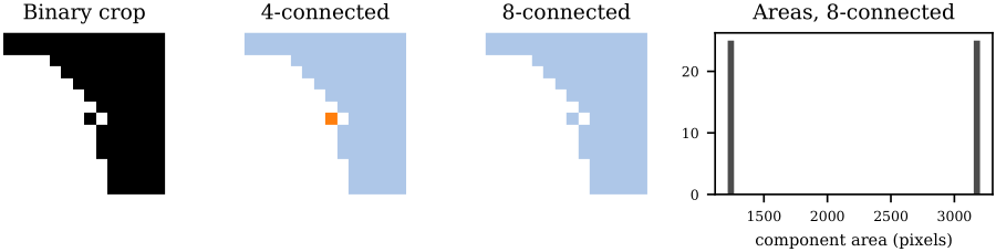
A 14-by-14 crop at the edge of a bolt. The diagonal pixel is its own 4-connected component (orange) but part of the bolt under 8-connectivity. Right: the 50 eight-connected areas fall into two tight clusters, nuts near 1200–1250 pixels and bolts near 3150–3200.
When it fails. Two objects that touch become one component (two nuts in contact count as one), and a highlight that cuts an object makes two. Threshold-plus-components is the right tool when objects are well separated, as on a clean conveyor; when they touch, reach for the watershed.
the watershed
the idea: flood the landscape
Read the image as terrain, with grey value as height. Pierce a hole at every local minimum and slowly lower the terrain into water. Each minimum fills its own catchment basin; wherever water from two basins is about to meet, build a dam. When everything is submerged, the dams are the watershed lines and the basins are the segments. On an image of cells with bright membranes, the dark interiors are basins and the dams land on the membranes.
- Give each marker (by default each local minimum) its own label, and push its neighbours onto a priority queue keyed by grey value, lowest first.
- Pop the lowest pixel \(p\). If all its labelled neighbours share one label, give \(p\) that label; if they disagree, leave \(p\) unlabelled, which makes it a dam.
- Push every neighbour of \(p\) that has never been queued, and repeat until the queue is empty.
Each pixel enters the queue once, so with a heap the cost is \(O(MN\log MN)\). The priority queue is what makes it behave like rising water: pixels flood in order of height.
Take \(I = (3,1,2,4,6,3,0,2,5,1)\) at positions \(p = 0, \dots, 9\). The minima at \(p = 1, 6, 9\) seed basins 1, 2 and 3. Popping lowest first (ties by arrival): \(p=2\) and \(p=7\) (height 2) join basins 1 and 2; \(p=0\) and \(p=5\) (height 3) join basins 1 and 2; \(p=3\) (height 4) joins basin 1. Then \(p=8\) (height 5) has neighbours in basins 2 and 3, so it becomes a dam, and \(p=4\) (height 6) sits between basins 1 and 2, another dam.
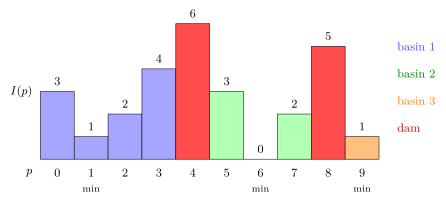
The flooded signal: labels \((1,1,1,1,\text{dam},2,2,2,\text{dam},3)\). The dams fall on the two local maxima, exactly where water from neighbouring basins first meets.
Since the segments are basins of minima, the objects must be the minima. Invert bright objects first, or run the watershed on the gradient magnitude: then object interiors and background are low, boundaries are ridges, and the dams land on the edges. For touching blobs in a binary mask, run it on the (negated) distance transform, which the Morphology page covers.
why it oversegments
Every local minimum becomes a basin, and real images have thousands of minima, nearly all of them noise. The raw watershed therefore shatters the image:
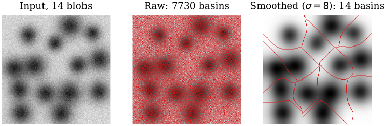
Fourteen dark blobs with additive noise. Middle: the raw image has 7730 regional minima, hence 7730 basins. Right: after Gaussian smoothing with \(\sigma = 8\), only the 14 blob minima survive and the watershed returns one region per blob. Intermediate smoothing gives 78 (\(\sigma=2\)), 22 (\(\sigma=4\)) and 16 (\(\sigma=6\)) basins.
Three standard remedies, often combined:
- Smooth first, so noise minima disappear (above).
- Merge afterwards, joining basins that are shallow, small, or separated by a low-contrast dam.
- Flood from markers instead of all minima: one marker per object, from the user, from a threshold, or from peaks of the distance transform. This is the most reliable, because it fixes the number of regions up front.
When it fails. Without smoothing or markers, always. Where an object has no ridge around it (a weak boundary), the floods from two basins meet in the wrong place.
When to use it. Splitting touching or overlapping objects whose boundaries are ridges (cells with bright membranes), or touching blobs via the distance transform. Use markers whenever you know roughly how many objects there are or where.
mean shift
the idea: climb the density
How would you segment a photograph of a street of painted houses by colour alone? Map every pixel to a point in a colour space and look for dense clusters: each cluster is one paint colour. \(K\)-means needs to be told how many clusters, is dragged by outliers (the mean is not robust) and gets stuck in local minima. Mean shift avoids all three by looking for the modes (peaks) of the point density directly: drop a window anywhere, move it to the centre of gravity of the points inside, and repeat until it stops moving.
- Start a window at a seed \(\mathbf x\).
- Replace \(\mathbf x\) by the kernel-weighted mean of the points in the window, \[ m(\mathbf x) = \frac{\sum_i K(\mathbf x_i - \mathbf x)\,\mathbf x_i}{\sum_i K(\mathbf x_i - \mathbf x)}, \qquad K(\mathbf d) = \exp\!\left(-\lVert \mathbf d\rVert^2/h^2\right) . \]
- Repeat until the mean-shift vector \(m(\mathbf x) - \mathbf x\) is negligible. The point reached is a mode.
To find every cluster, seed on a regular grid, run all seeds to convergence, merge seeds that land close together, and label each data point by the mode its own seed reaches. The single parameter is the bandwidth \(h\).
Why does a moving average find peaks? Because it is gradient ascent in disguise.
Let \(\hat p(\mathbf x) = c\sum_i \exp(-\lVert \mathbf x_i - \mathbf x\rVert^2/h^2)\) be the Gaussian kernel density estimate of the points. Then \[ m(\mathbf x) - \mathbf x = \frac{h^2}{2}\,\frac{\nabla \hat p(\mathbf x)}{\hat p(\mathbf x)} . \] Each step goes straight uphill on the smoothed density, with long strides where the density is low and short ones near a peak, and the iteration stops exactly at stationary points of \(\hat p\).
Points \(\{1, 2, 3, 7, 8, 9.5\}\); flat kernel on the window \([x-2, x+2]\), so \(m(x)\) is the plain mean of the points inside.
- Seed \(x = 4\): window \([2,6]\) holds 2, 3, so \(m = 2.5\); window \([0.5, 4.5]\) holds 1, 2, 3, so \(m = 2\); no further shift. Mode at 2.
- Seed \(x = 6\): window \([4,8]\) holds 7, 8, so \(m = 7.5\); window \([5.5, 9.5]\) holds 7, 8, 9.5, so \(m = 8.1\overline{6}\); the window now holds the same three points. Mode at \(8.1\overline{6}\).
Two clusters, \(\{1,2,3\}\) and \(\{7,8,9.5\}\), found without being told \(K = 2\). With a window of radius 1 the same seeds stop at 2.5 and 7.5: the modes depend on the bandwidth.
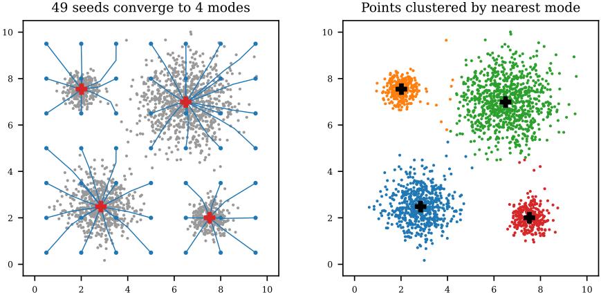
2100 points from four Gaussian clusters of very different sizes. All 49 seeds of a 7-by-7 grid climb (blue) to one of 4 modes (red), each within 0.05 of a true cluster centre. Right: the points labelled by mode. Gaussian kernel, \(h = 1\).
To segment an image, use colour (and texture or gradients) as features, usually with the pixel coordinates appended so segments come out spatially coherent; then run mean shift and paint each pixel with its mode’s colour. The result is the familiar posterised “mean-shift art”.
| strengths | weaknesses |
|---|---|
| assumes no cluster shape | many windows to shift: slow |
| finds the number of clusters | result depends on bandwidth |
| one parameter | bandwidth is hard to choose |
| robust to outliers | poor in high dimensions |
The last weakness is the curse of dimensionality: in many dimensions a fixed-radius window holds almost no points, and the density estimate falls apart.
When to use it. Colour or colour-plus-position segmentation where the number of regions is unknown and the feature space is low-dimensional. If you know \(K\) and want speed, \(K\)-means is fine; if you want a fast first pass over a big image, use superpixels.
proofs
By the chain rule each term of \(\hat p\) has gradient \(\frac{2}{h^2}K(\mathbf x_i - \mathbf x)(\mathbf x_i - \mathbf x)\). Summing, \[ \nabla\hat p(\mathbf x) = \frac{2c}{h^2}\Big(\sum_i K(\mathbf x_i - \mathbf x)\Big)\big(m(\mathbf x) - \mathbf x\big) = \frac{2}{h^2}\,\hat p(\mathbf x)\,\big(m(\mathbf x) - \mathbf x\big) , \] which rearranges to the claim. Truncating the sums to a finite window drops only negligible terms of the Gaussian.
SLIC superpixels
the idea: oversegment on purpose
Mean shift and graph methods are expensive per pixel. A superpixel method groups similar neighbouring pixels into a few hundred small, compact patches that hug edges. The result is a deliberate oversegmentation: each object is covered by several superpixels, but ideally no superpixel straddles a boundary. Everything downstream (classification, merging, a CRF) then works on hundreds of units instead of \(10^5\) pixels.
Simple linear iterative clustering (SLIC) is \(K\)-means on five-dimensional points \((l, a, b, x, y)\), colour in CIELAB plus position, with two changes: a distance that balances colour against position, and a search restricted to a window around each centre.
- Place cluster centres on a grid with step \(S\) (target superpixel size about \(S \times S\)), then nudge each to the lowest-gradient pixel in its 3-by-3 neighbourhood, so no centre starts on an edge.
- For each centre, examine only the pixels in the \(2S \times 2S\) window around it, and assign each pixel to the centre with the smallest \[ D = \sqrt{\frac{d_{lab}^2}{m^2} + \frac{d_{xy}^2}{S^2}} , \] where \(d_{lab}\) is the colour distance and \(d_{xy}\) the pixel distance.
- Recompute each centre as the mean colour and position of its pixels; repeat until the centres stop moving.
Every design choice has a reason. Dividing by \(m\) and \(S\) makes the two distances unit-free; a large compactness \(m\) lets position dominate, giving regular honeycomb cells, while a small \(m\) lets cells chase colour edges. The window is the “linear” in the name: about \(MN/S^2\) centres each look at \(4S^2\) pixels, so an iteration costs about \(4MN\) distance evaluations whatever the number of superpixels, where plain \(K\)-means would compare every pixel with every centre.
\(S = 16\), \(m = 10\). Centre colour \((50, 10, 20)\) at \((40, 40)\); pixel colour \((55, 13, 16)\) at \((48, 46)\). Then \(d_{lab} = \sqrt{25 + 9 + 16} = \sqrt{50}\) and \(d_{xy} = \sqrt{64 + 36} = 10\), so \[ D = \sqrt{\frac{50}{100} + \frac{100}{256}} = \sqrt{0.500 + 0.391} = 0.944 . \] Colour and position contribute comparably, which is precisely the balance \(m\) and \(S\) are chosen to strike.
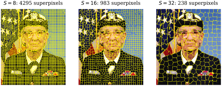
SLIC with compactness \(m = 10\) at grid steps \(S = 8, 16, 32\). The cells follow the cap, glasses and medals. Small fragments are merged away, so the counts (4295, 983, 238) fall a little below \(MN/S^2\).
When it fails. SLIC never produces a whole object, by design. Structures thinner than \(S\) (a wire, a neurite) get absorbed into their surroundings, and with large \(m\) weak colour edges are crossed.
When to use it. As a fast, memory-light front end that turns an image into a few hundred coherent units for a classifier or a CRF. Pick \(S\) below the size of the smallest object you care about.
graph cuts and conditional random fields
the idea: data plus smoothness
Classify each superpixel on its own and the answer is noisy: a patch of a cow’s leg may look more like grass than cow. But it is adjacent to, and similar to, patches that are confidently cow. A conditional random field puts both kinds of evidence into one energy over a labelling \(c\) of the superpixels \(s_i\) (see probabilistic graphical models for the general machinery): \[ E( c) = \sum_i \varphi(s_i, c_i) + \sum_{i \sim j} \psi(s_i, s_j) . \]
- The unary term \(\varphi(s_i, c)\) is the cost of giving superpixel \(i\) class \(c\), typically \(-\log P(c \mid s_i)\) from a classifier.
- The pairwise term charges \(w_{ij} \ge 0\) when adjacent superpixels get different classes and nothing otherwise, with \(w_{ij}\) larger the more similar they are. Cutting between similar neighbours is expensive; cutting along a real edge is cheap.
Since the probability of a labelling is proportional to \(e^{-E}\), the minimum-energy labelling is the most probable one.
Superpixels \(s_1 - s_2 - s_3\) in a row; classes 0 (background) and 1 (object). Unary costs \((\varphi(\cdot,0), \varphi(\cdot,1))\) are \(s_1 : (4,1)\), \(s_2 : (2,3)\), \(s_3 : (1,5)\). Pairwise weights \(w_{12} = 3\) (similar) and \(w_{23} = 1\) (dissimilar).
| \(c\) | unary | pairwise | \(E\) |
|---|---|---|---|
| 000 | 7 | 0 | 7 |
| 001 | 11 | 1 | 12 |
| 010 | 8 | 4 | 12 |
| 011 | 12 | 3 | 15 |
| 100 | 4 | 3 | 7 |
| 101 | 8 | 4 | 12 |
| 110 | 5 | 1 | 6 |
| 111 | 9 | 0 | 9 |
The minimum is \(E = 6\) at \(c = (1,1,0)\). On its own data \(s_2\) prefers background (\(2 < 3\)), and labelling each superpixel greedily gives \((1,0,0)\) with \(E = 7\). The strong tie to the object superpixel \(s_1\) pulls \(s_2\) into the object: that is what the smoothness term is for.
min-cut solves it exactly
Enumeration costs \(2^n\) labellings. For two classes, the minimum is found exactly in polynomial time by turning the energy into a flow network. Add a source terminal \(s\) (background) and a sink \(t\) (object); join every node to both terminals and adjacent nodes to each other. A cut removes edges until no path joins \(s\) to \(t\); nodes left with \(s\) are background, nodes left with \(t\) are object.
Give edge \(s \to i\) capacity \(\varphi(s_i, 1)\), edge \(i \to t\) capacity \(\varphi(s_i, 0)\), and the link \(i - j\) capacity \(w_{ij}\). Then for every labelling, the capacity of the corresponding cut equals \(E( c)\). So a minimum cut is a minimum-energy labelling, and by the max-flow min-cut theorem it can be found by computing a maximum flow.
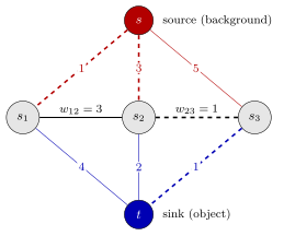
The network for the three-superpixel example. The minimum cut (dashed, total \(1 + 3 + 1 + 1 = 6\)) leaves \(s_1, s_2\) with the sink and \(s_3\) with the source: the labelling \((1,1,0)\), matching the enumeration.
With more than two classes exact minimisation is hard in general; one uses a terminal per class or repeated two-class moves. A group photograph can be cut into one segment per person this way.
When it fails. The answer is only as good as the potentials: a confidently wrong classifier on a whole region cannot be rescued by smoothness, and too large a pairwise weight deletes thin or small objects, because a short boundary is always cheaper.
When to use it. Whenever noisy per-pixel or per-superpixel decisions should be made spatially consistent, and for interactive foreground extraction from a few user strokes (the strokes fix some unary costs to infinity).
proofs
A cut separating the label-0 nodes (source side) from the label-1 nodes (sink side) must sever, for each node, the terminal edge that would join it to the opposite terminal, and every neighbour link whose ends lie on opposite sides.
- A node with \(c_i = 0\) stays with \(s\), so \(i \to t\) is cut: cost \(\varphi(s_i, 0)\).
- A node with \(c_i = 1\) stays with \(t\), so \(s \to i\) is cut: cost \(\varphi(s_i, 1)\).
- The link \(i - j\) is cut exactly when \(c_i \neq c_j\): cost \(w_{ij}\).
Adding up gives \(\sum_i \varphi(s_i, c_i) + \sum_{c_i \neq c_j} w_{ij} = E( c)\).
scoring a segmentation
Every score compares a segmented object set \(\mathcal S\) with a hand-drawn ground truth \(\mathcal T\), pixel by pixel. Each pixel lands in one cell of a confusion matrix:
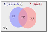
True positives \(\mathrm{TP} = \mathcal S \cap \mathcal T\), false positives \(\mathrm{FP} = \mathcal S \setminus \mathcal T\), false negatives \(\mathrm{FN} = \mathcal T \setminus \mathcal S\), and true negatives outside both.
sensitivity, specificity and ROC
Sensitivity \(\mathrm{TP}/(\mathrm{TP}+\mathrm{FN})\) is the fraction of the true object found; specificity \(\mathrm{TN}/(\mathrm{TN}+\mathrm{FP})\) is the fraction of true background kept as background. Each alone is trivially perfect (segment everything, or nothing), so they are reported together. A method with a knob, such as a threshold, traces a ROC curve of sensitivity against \(1 - \) specificity as the knob turns, and the area under it (AUC) ranks methods: 1 is perfect, 0.5 is guessing.
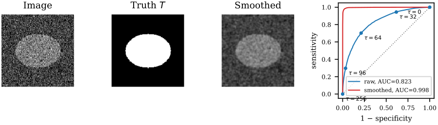
A bright ellipse (mean 80) on a noisy background (mean 40, noise s.d. 30), thresholded at every (tau). Raw: AUC 0.823. After a Gaussian smooth with (sigma = 1): AUC 0.998. The smoothed curve lies above the raw one everywhere, so “smooth, then threshold” wins at every operating point.
Dice and Jaccard
Segmentation usually has a tiny object in a sea of background, and anything that counts true negatives is flattered by the sea. The two standard scores measure the overlap of \(\mathcal S\) and \(\mathcal T\) directly and ignore TN.
\[ J = \mathrm{IoU}(\mathcal S, \mathcal T) = \frac{|\mathcal S \cap \mathcal T|}{|\mathcal S \cup \mathcal T|} = \frac{\mathrm{TP}}{\mathrm{TP} + \mathrm{FP} + \mathrm{FN}} . \]
\[ D = \frac{2|\mathcal S \cap \mathcal T|}{|\mathcal S| + |\mathcal T|} = \frac{2\,\mathrm{TP}}{2\,\mathrm{TP} + \mathrm{FP} + \mathrm{FN}} . \]
Both are 1 for a perfect match and 0 for no overlap. They are not rivals:
Whenever \(\mathcal S \cup \mathcal T\) is non-empty,
- \(D = F_1\), the harmonic mean of precision and recall;
- \(D = 2J/(1+J)\) and \(J = D/(2-D)\);
- \(J \le D\), with equality only at \(J = 0\) or \(J = 1\).
So Dice and Jaccard always rank segmentations the same way, and Dice is always the bigger number: \(J = 0.5\) means \(D = 2/3\).
A 1000-pixel image holds a 60-pixel object. A method marks 50 pixels, 40 of them on the object. So \(\mathrm{TP} = 40\), \(\mathrm{FP} = 10\), \(\mathrm{FN} = 20\), \(\mathrm{TN} = 930\).
| score | value |
|---|---|
| sensitivity | \(40/60 = 0.667\) |
| specificity | \(930/940 = 0.989\) |
| precision | \(40/50 = 0.800\) |
| Dice | \(80/110 = 0.727\) |
| Jaccard | \(40/70 = 0.571\) |
Specificity looks superb although a third of the object is missing: the background inflates it. Dice equals \(F_1 = 2(0.8)(0.667)/1.467 = 0.727\), and \(2J/(1+J) = 1.143/1.571 = 0.727\) checks the conversion. Jaccard is the harshest of the lot.
Which to report. ROC and AUC when tuning a parameter and the background is not overwhelming; Dice or Jaccard (pick one, they carry the same information) when the object is small relative to the image, which in medical imaging is almost always. The same IoU scores bounding boxes in object detection.
proofs
For the first claim, substitute \(P = \mathrm{TP}/(\mathrm{TP}+\mathrm{FP})\) and \(R = \mathrm{TP}/(\mathrm{TP}+\mathrm{FN})\) into \(F_1 = 2PR/(P+R)\) and multiply through by \((\mathrm{TP}+\mathrm{FP})(\mathrm{TP}+\mathrm{FN})\): \[ F_1 = \frac{2\,\mathrm{TP}^2}{\mathrm{TP}(\mathrm{TP}+\mathrm{FP}) + \mathrm{TP}(\mathrm{TP}+\mathrm{FN})} = \frac{2\,\mathrm{TP}}{2\,\mathrm{TP}+\mathrm{FP}+\mathrm{FN}} = D . \] For the second, write \(u = \mathrm{FP} + \mathrm{FN}\), so \(J = \mathrm{TP}/(\mathrm{TP}+u)\) and \(1 + J = (2\,\mathrm{TP}+u)/(\mathrm{TP}+u)\); dividing gives \(2J/(1+J) = 2\,\mathrm{TP}/(2\,\mathrm{TP}+u) = D\), and solving \(D(1+J) = 2J\) gives \(J = D/(2-D)\). For the third, \[ D - J = \frac{2J}{1+J} - J = \frac{J(1-J)}{1+J} \ge 0 \quad\text{for } 0 \le J \le 1 , \] with equality only at the endpoints.
choosing a method
| method | bets on | breaks on |
|---|---|---|
| Otsu threshold | two separated humps | overlap, skew, shading |
| connected components | objects apart | touching objects |
| watershed | ridges between objects | noise minima, weak edges |
| mean shift | dense colour clusters | high dimensions, speed |
| SLIC | local colour coherence | thin structures |
| graph cut / CRF | a decent unary classifier | confident unary errors |
The pipelines that work chain these: threshold, clean with morphology, split touching blobs with a marker watershed, count components; or superpixels, a classifier per superpixel, a CRF for consistency. Two families are left out here: region growing and split-and-merge (local homogeneity tests from a seed or a quadtree), and contour methods (snakes and level sets) that fit the boundary curve itself. Learned segmenters replace the hand-made unary term with a convolutional network, and they are judged with exactly the Dice and IoU scores above.
Further reading: Szeliski, Computer Vision: Algorithms and Applications (2nd ed.), §3.3.3 (thresholding), §7.5 (split and merge, watershed, mean shift), §4.3 (Markov random fields and graph cuts).
see also
- Morphology – cleaning masks and splitting touching blobs before counting
- Semantic and Instance Segmentation – the learned, per-pixel successors to these methods
- Object Detection – where the same IoU scores bounding boxes
Backlinks (5)
1. Morphology: Counting Nuts and Bolts /wiki/computer-vision/morphology/
2. Motion and Tracking /wiki/computer-vision/motion-tracking/
3. Object Detection /wiki/computer-vision/detection/
4. Semantic and Instance Segmentation /wiki/computer-vision/dense-prediction/
5. Computer Vision /wiki/computer-vision/
I think taking a course in a subject that you are interested in is never particularly a bad thing.
Comments