SIFT, Matching and Stitching

Take two photographs of the same building from slightly different spots. To glue them into one panorama you need three things: points that can be found again in both pictures, a way of deciding which point in one picture is which point in the other, and the single geometric map that carries one picture onto the other even though some of those decisions are wrong. The scale-invariant feature transform (SIFT) of Lowe (2004) supplies the first two; a homography fitted by random sample consensus (RANSAC) supplies the third. 𐃏

The whole pipeline ends in one comparison that is worth keeping in mind from the start. On two overlapping views of a castle, a homography fitted by RANSAC reprojects its inliers with a median error of 0.18 pixels; a homography fitted by plain least squares to all the matches misses the same points by a median 5.60 pixels. Every section below is about earning that factor of 30.

scale space and DoG extrema

A corner photographed from twice as far away is half as large. A detector with one fixed window finds it in one image and misses it in the other, so SIFT does not choose a size: it searches all of them at once.

the scale space

Blur the image with Gaussians of growing width. The stack of blurred images is the scale space \[ L(x,y,\sigma) = G_\sigma * I(x,y), \qquad G_\sigma(x,y) = \frac{1}{2\pi\sigma^2}e^{-(x^2+y^2)/(2\sigma^2)} . \] Fine detail lives at small $\sigma$ and is gone by large $\sigma$; big structures only stand out once the small ones have been blurred away. Subtracting neighbouring levels isolates what exists at one particular scale.

Definition (Difference of Gaussians)

For $\sigma_1 < \sigma_2$ and weights $a_1, a_2 > 0$, the difference of Gaussians is the kernel \[ \mathrm{DoG} = a_1 G_{\sigma_1} - a_2 G_{\sigma_2} , \] a narrow positive peak sitting in a wide negative trough. SIFT uses equal weights and adjacent scales a factor $k$ apart, with the sign reversed: \[ D(x,y,\sigma) = L(x,y,k\sigma) - L(x,y,\sigma) = \bigl(G_{k\sigma} - G_\sigma\bigr) * I(x,y) . \]

With equal weights the kernel sums to zero, so flat regions give zero response; both Gaussians die off at high frequency, so pixel noise is suppressed too. A DoG is a band-pass filter: it answers to one band of sizes, which is exactly what a scale detector wants. The frequency-domain view is on the Seeing in Frequency page.

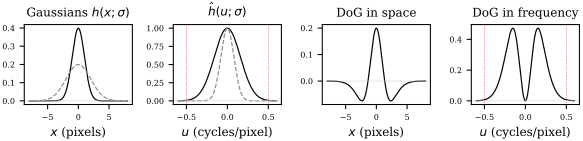
$A DoG with $\sigma_1=1$, $\sigma_2=2$ pixels in space and in frequency. The response is zero at $u=0$, peaks at $0.153$ cycles per pixel, and is almost zero at the Nyquist frequency $0.5$: band-pass, not high-pass.$

A DoG with $\sigma_1=1$, $\sigma_2=2$ pixels in space and in frequency. The response is zero at $u=0$, peaks at $0.153$ cycles per pixel, and is almost zero at the Nyquist frequency $0.5$: band-pass, not high-pass.

Why is the DoG the right thing to look at? Because it is, almost for free, the Laplacian of Gaussian (LoG), the classic blob detector, already normalised so that responses at different scales can be compared.

Proposition (DoG approximates the scale-normalised Laplacian)

For $k$ close to 1, \[ G_{k\sigma} - G_\sigma \approx (k-1)\,\sigma^2\,\nabla^2 G_\sigma . \]

The factor $\sigma^2$ is the scale normalisation that makes extrema at different $\sigma$ comparable, and the factor $k-1$ is the same at every level, so it never moves an extremum. The DoG costs one image subtraction, because both blurred images are already in the scale space. A blob of radius about $\sqrt2\,\sigma$ gives the strongest response.

octaves and the 26-neighbour test

Lowe’s design puts $n_s = 3$ intervals in each octave (a doubling of $\sigma$), so $k = 2^{1/3}$, and halves the image after every octave, exactly as a Gaussian pyramid does. A sample of $D$ becomes a candidate keypoint when it is larger than all, or smaller than all, of its 26 neighbours: 8 around it in its own level and 9 in each of the levels above and below. The winner gives a position and a scale.

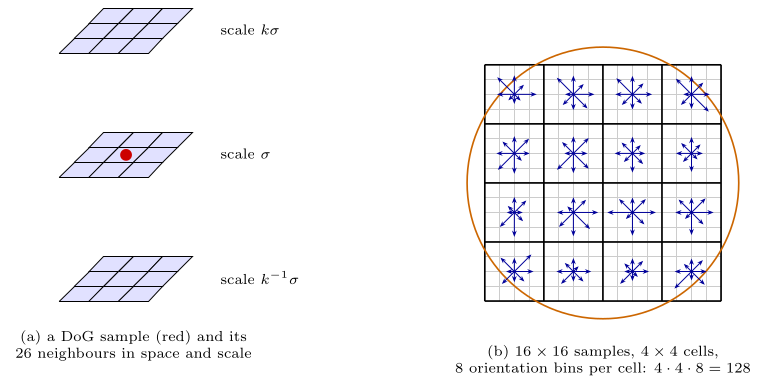
(a) The extremum test compares a DoG sample with 26 neighbours in space and scale. (b) The descriptor layout used later: a $16\times16$ window split into $4\times4$ cells, each holding an 8-bin orientation histogram; the circle is the Gaussian weighting window.

Example (One octave on the castle)

A $240\times240$ crop of the castle facade, blurred at $\sigma = 1.6\,k^j$ with $k=\sqrt2$ (a coarser $k$ than Lowe’s, to make the levels visibly different). In the DoG row, grey is zero. At $\sigma = 1.6$ the window frames, dormers and stonework light up; by $\sigma = 4.53$ only whole windows, dormers and turrets respond. A window corner is an extremum at one scale, a whole window at another, and the 26-neighbour test finds each at its own level.

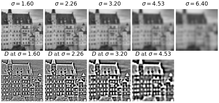
Top: the scale space $L(x,y,\sigma)$ on a crop of the Lab 1 castle image. Bottom: the four DoG images $D = L(k\sigma) - L(\sigma)$, grey $=0$.

proofs

Proof (DoG approximates the scale-normalised Laplacian)

Heat equation. With $r^2 = x^2 + y^2$, differentiating $G_\sigma$ in $\sigma$ gives \[ \frac{\partial G_\sigma}{\partial\sigma} = \frac{r^2 - 2\sigma^2}{\sigma^3}\,G_\sigma , \] while differentiating twice in space gives \[ \nabla^2 G_\sigma = \frac{r^2 - 2\sigma^2}{\sigma^4}\,G_\sigma . \] So $\partial G_\sigma / \partial\sigma = \sigma\,\nabla^2 G_\sigma$.

Finite difference in $\sigma$. For $k$ close to 1, \[ \frac{\partial G_\sigma}{\partial\sigma} \approx \frac{G_{k\sigma} - G_\sigma}{k\sigma - \sigma} . \]

Combine. \[ G_{k\sigma} - G_\sigma \approx (k-1)\sigma \cdot \sigma\,\nabla^2 G_\sigma = (k-1)\,\sigma^2\,\nabla^2 G_\sigma . \]

from extrema to keypoints

The raw extrema are accurate only to one pixel and one scale level, and most of them are junk: faint ripples in the sky, or points strung along an edge. Three refinements turn candidates into keypoints.

Sub-pixel position: Expand $D$ to second order about the sample in $\mathbf x = (x, y, \sigma)^\top$ and set the derivative to zero. The true extremum sits at the offset \[ \hat{\mathbf x} = -\Bigl(\frac{\partial^2 D}{\partial \mathbf x^2}\Bigr)^{-1}\frac{\partial D}{\partial \mathbf x} . \]
Low contrast: If $|D(\hat{\mathbf x})| < 0.03$ (grey values in $[0,1]$) the extremum is too weak to survive noise, and it is dropped.
Edges: On an edge the DoG curves sharply across the edge and hardly at all along it, so the point can slide along the edge. Keep the point only if the ratio of the principal curvatures is below $r = 10$. That needs only the trace and determinant of the spatial Hessian of $D$: \[ \frac{(D_{xx} + D_{yy})^2}{D_{xx}D_{yy} - D_{xy}^2} < \frac{(r+1)^2}{r} = 12.1 . \]

What survives sits on corners and blobs, the places whose position is pinned down in both directions. The edge test is the Harris idea (see Motion and Tracking) applied to the DoG instead of to the gradient structure tensor.

orientation and the 128-d descriptor

A keypoint so far is $(x, y, \sigma)$. To compare it with keypoints in a rotated copy of the image, it needs a frame that rotates with the object, and then a summary of what the neighbourhood looks like in that frame.

orientation assignment

Around the keypoint, at its own scale, compute the gradient of $L$ at every pixel: \[ M = \sqrt{G_x^2 + G_y^2}, \qquad \theta = \operatorname{atan2}(G_y, G_x) . \] Each pixel votes into a 36-bin histogram of $\theta$ (bins of $10^\circ$) with weight $M$ times a Gaussian that favours pixels near the centre. The highest peak is the keypoint’s orientation. Every other peak above 80% of it spawns a second keypoint at the same place and scale with that orientation, so a corner with two strong edge directions yields two keypoints. The two-argument $\operatorname{atan2}$ matters: $\tan^{-1}(G_y/G_x)$ covers only $180^\circ$ and cannot tell a dark-to-light edge from a light-to-dark one.

the descriptor

Take a $16\times16$ window, rotated to the keypoint orientation and scaled with $\sigma$, and cut it into a $4\times4$ grid of cells (panel (b) of the figure above).

In each cell, histogram the gradient orientations, measured relative to the keypoint orientation, into 8 bins of $45^\circ$, weighted by magnitude and by a Gaussian centred on the keypoint.
Concatenate the 16 histograms: $4 \times 4 \times 8 = 128$ numbers, the descriptor $\mathbf d \in \mathbb R^{128}$.
Normalise $\mathbf d$ to unit length, clip every entry at $0.2$, and normalise again.

Each design choice buys a specific robustness. Gradients ignore a constant brightness offset. Unit length cancels an overall contrast change, which scales every gradient equally. The clip at $0.2$ stops a few huge gradients (glare, a specular highlight) from dominating. The coarse $4\times4$ spatial binning tolerates a pixel or two of shift and a little affine distortion.

the whole algorithm

Definition (Algorithm: SIFT)

Input: a grey image $I$. Output: keypoints $(x, y, \sigma, \theta)$, each with a descriptor $\mathbf d \in \mathbb R^{128}$.

Scale-space extrema. Build $L(x,y,\sigma) = G_\sigma * I$ over scales $\sigma, k\sigma, k^2\sigma, \dots$, octave by octave, and the differences $D = L(k\sigma) - L(\sigma)$. Keep every sample that beats all 26 neighbours. This gives location and scale.
Keypoint localisation. Refine to sub-pixel and sub-scale accuracy by a quadratic fit; discard low-contrast points and edge points.
Orientation assignment. The main peak of the magnitude-weighted gradient-orientation histogram gives $\theta$; each peak above 80% of it adds a keypoint. This gives rotation invariance.
Descriptor. In a window aligned with $\theta$ and sized by $\sigma$, build a $4\times4$ array of 8-bin orientation histograms, concatenate, normalise, clip at 0.2, renormalise.

OpenCV’s defaults: 3 scales per octave, initial $\sigma = 1.6$, contrast threshold 0.04, edge threshold $r = 10$.

A classic confusion is worth naming. Scale invariance comes from the search over $\sigma$ in step 1. Rotation invariance comes from the orientation assignment in step 3, not from the multi-scale search. Illumination robustness comes from the normalised gradients in step 4.

Example (SIFT on two views of the castle)

Two $330\times430$ views of the castle (the left part of the image, and a second view made from the image by a known homography, built in the stitching section below), through OpenCV’s SIFT_create() with default parameters:

view 1 gives 1407 keypoints, so a $1407\times128$ descriptor array; view 2 gives 1715;
raising the contrast threshold from 0.04 to 0.11 keeps 471 and 424, so the low-contrast cut of step 2 is the main knob on how many keypoints you get;
the median keypoint diameter is 2.7 pixels and the largest are near 94 pixels: fine detail is what a photograph has most of.

The 20 strongest keypoints (largest $|D|$) sit on spire tips and high-contrast window details, the points most likely to be found again in the other view.

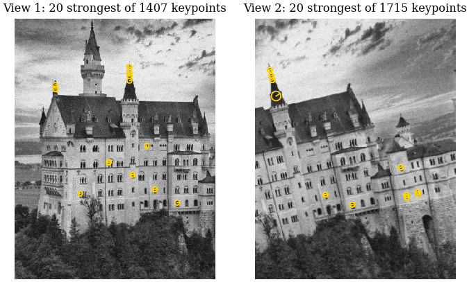
The 20 strongest SIFT keypoints of each castle view (view 2 is synthetic: the castle under a known homography). Circle radius shows the keypoint’s scale (at least 4 pixels, for visibility); the radius line shows its orientation.

how invariant is it, really

Invariance on paper says the keypoints move with the image. In practice resampling creates and destroys fine-scale extrema, so the honest question is how many keypoints come back, and whether the matches that come back are right.

Example (Scaling, rotation and noise)

The Lab 1 castle image ($512\times512$) is scaled by 1.2, rotated $60^\circ$ clockwise, or hit with 2% salt-and-pepper noise (seed 9517), and SIFT is rerun. Since each change is known, every original keypoint can be mapped to where it should land. Repeatability is the fraction of mapped keypoints with a detected keypoint within 2 pixels; correct is the fraction of ratio-test matches (threshold 0.8) landing within 3 pixels of the truth.

change	repeatability	matches	correct
none	1.00	2586	1.00
scale 1.2	0.76	1797	0.98
rotate 60 deg	0.77	1579	0.97
2% salt, pepper	0.66	1408	0.97

Two thirds to three quarters of the keypoints survive each change, and 97% or more of the surviving matches are correct. SIFT is invariant in the sense that matters for matching, not in the sense that every keypoint survives. (The scaled image has 4184 keypoints, against 2586: a bigger image has more fine-scale extrema. Impulse noise adds spurious ones too.)

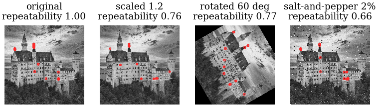
The 20 strongest keypoints of the castle image after each change, with the repeatability of all keypoints.

when SIFT fails

No texture. Blank walls and sky give almost no keypoints.
Repeated structure. Identical windows on a facade have near-identical descriptors, so the ratio test (next section) throws away true matches and lets some false ones through.
Big viewpoint change. The invariance is to similarity transforms plus mild affine distortion. Beyond roughly $30^\circ$ to $40^\circ$ out of plane, or under non-rigid deformation, the descriptors change and matching collapses.
Speed. 128 floating-point numbers per keypoint, thousands of keypoints per image, is slow by real-time standards.

when to use it vs alternatives

Use SIFT to match distinctive points between views of a rigid, textured scene: stitching, structure from motion, object instance recognition. For whole-image retrieval or classification a global colour or texture descriptor (or a bag of SIFT words) is the better tool. When speed matters more than accuracy, binary descriptors (ORB, BRISK) compared by Hamming distance are an order of magnitude faster. Learned CNN features now beat hand-crafted ones on hard viewpoint and lighting changes, at the cost of a trained network.

matching with the ratio test

With descriptors in both images, the obvious rule pairs each descriptor with its nearest neighbour in the other image (Euclidean distance in $\mathbb R^{128}$). The trouble is that every descriptor has a nearest neighbour, including those of points that are not in the other image at all. Something must decide whether the nearest neighbour is a genuine match.

Definition (Nearest-neighbour distance ratio)

For a descriptor $\mathbf d_A$ in image 1, let $d_1$ and $d_2$ be its distances to the nearest and second-nearest descriptors in image 2. Accept the nearest match when \[ \frac{d_1}{d_2} \le 0.8 , \] and reject it otherwise. (Lab 2 uses the stricter 0.75.)

Why a ratio rather than a cap on $d_1$? Descriptor distances vary a lot from one part of an image to another, so no single cap works everywhere. The ratio asks a relative question: is the best candidate clearly better than the runner-up? A true match has one close neighbour and the rest far away, so $d_1 \ll d_2$. A point with no partner, or a point on a repeated pattern, has several neighbours at similar distances, so $d_1 \approx d_2$. Lowe found that 0.8 throws out about 90% of false matches while losing under 5% of correct ones.

Example (Ratio beats an absolute threshold)

Three descriptors with their nearest and second-nearest distances:

$d_1$	$d_2$	ratio	verdict
0.30	0.45	0.67	accept
0.40	0.44	0.91	reject
0.50	0.90	0.56	accept

An absolute cap of $d_1 \le 0.45$ would keep the second (ambiguous: two candidates almost equally close) and lose the third (distinctive: the runner-up is nearly twice as far). On the two castle views, 573 of view 1’s 1407 descriptors pass at ratio 0.8, and 541 at 0.75.

Even after the ratio test some matches are wrong; on the castle views the known homography shows that 20 of the 541 are (more than 3 pixels from where they should land). Matching alone cannot fix that. What fixes it is geometry: the right matches all agree on one transformation, and the wrong ones agree on nothing.

the homography

A spatial transformation maps $(x, y)$ in one image to $(x’, y’)$ in the other. Pick the family by what it must preserve:

family	keeps	dof	min pairs
translation	everything	2	1
rigid	lengths, angles	3	2
similarity	angles, shape	4	2
affine	parallel lines	6	3
homography	straight lines	8	4

Each family contains the ones above it, and each correspondence supplies two equations, which is where the minimum number of pairs comes from.

Definition (Homography)

In homogeneous coordinates (a point $(x,y)$ written as $(x, y, 1)^\top$), a homography is an invertible map \[ \begin{pmatrix} x’ \\ y’ \\ w’ \end{pmatrix} = \mathbf H \begin{pmatrix} x \\ y \\ 1 \end{pmatrix}, \qquad \mathbf H = \begin{pmatrix} h_{11} & h_{12} & h_{13} \\ h_{21} & h_{22} & h_{23} \\ h_{31} & h_{32} & h_{33} \end{pmatrix}, \] with image point $(x’/w’, y’/w’)$. Since $\mathbf H$ and $\lambda\mathbf H$ give the same map, it has $9 - 1 = 8$ degrees of freedom; fix $h_{33} = 1$ or $\|\mathbf H\| = 1$.

Two facts make the homography the model for panoramas. Two images of a planar scene are related exactly by a homography, and so are two images taken by a camera that only rotates about its centre: with intrinsic matrix $\mathbf K$ and rotation $\mathbf R$, $\mathbf H = \mathbf K \mathbf R \mathbf K^{-1}$. The bottom row $(h_{31}, h_{32})$ is what makes it projective: points further along that direction are divided by a larger $w’$ and shrink.

To estimate $\mathbf H$, clear the denominator in \[ x’ = \frac{h_{11}x + h_{12}y + h_{13}}{h_{31}x + h_{32}y + h_{33}} \] and in the matching formula for $y’$. Each pair gives two equations linear in the nine entries. Stack $n \ge 4$ pairs into a $2n \times 9$ homogeneous system and take the right singular vector of the smallest singular value: the direct linear transform (DLT). See the Linear Algebra page for the singular value decomposition.

Example (A square that no affine map can reach)

Send the corners $(0,0), (1,0), (1,1), (0,1)$ of the unit square to $(0,0), (\tfrac12, 0), (\tfrac12, \tfrac12), (0, 1)$.

No affine map can: an affine map sends a square to a parallelogram, but here the images of the sides $x=0$ and $x=1$ have lengths 1 and $\tfrac12$. Try \[ \mathbf H = \begin{pmatrix} 1 & 0 & 0 \\ 0 & 1 & 0 \\ 1 & 0 & 1 \end{pmatrix}, \qquad (x, y) \mapsto \Bigl(\frac{x}{x+1}, \frac{y}{x+1}\Bigr) . \] All four corners land where they should. The $8\times9$ DLT system for these pairs has rank 8 (smallest singular value $0.18$), so this $\mathbf H$ is the only one with $h_{33} = 1$. The right-hand side, $x = 1$, is divided by $w’ = 2$ and shrinks: that is perspective.

RANSAC

why least squares is not enough

Least squares picks the parameters minimising $\sum_i \|T(\mathbf x_i) - \mathbf x_i’\|^2$ (see Ordinary Least Squares). Squared error rewards dragging the fit towards a gross error, so one false match can move the answer arbitrarily far.

Example (One bad match ruins a translation)

Points $A_1 = (2,3)$, $A_2 = (5,1)$, $A_3 = (4,6)$ are matched to $B_1 = (5,4)$, $B_2 = (8,2)$, $B_3 = (10,4)$. For a pure translation the least-squares answer is the mean displacement. The displacements are $(3,1)$, $(3,1)$, $(6,-2)$, so \[ \hat{\mathbf t} = \tfrac13\bigl((3,1) + (3,1) + (6,-2)\bigr) = (4, 0) . \] Two pairs agree on $(3,1)$; the third is a false match, and it has dragged the estimate a full unit in each coordinate, so it fits none of the pairs.

the algorithm

RANSAC (Fischler and Bolles, 1981) turns the problem round. Instead of fitting everything and hoping, fit the model to the smallest possible random subset and let the rest of the data vote.

Definition (Algorithm: RANSAC)

Input: data (here, correspondences); a model needing $s$ data for an exact fit; an inlier threshold $\delta$; an iteration count $N$.

Repeat $N$ times:
1. draw a random sample of $s$ data (translation $s=1$, line $s=2$, affine $s=3$, homography $s=4$);
2. fit the model exactly to the sample;
3. count the inliers, the data within distance $\delta$ of the model;
4. if the count beats the best so far, keep this model.
Refit the best model by least squares on its inliers.
Return the refitted model and its inliers.

Example (RANSAC rescues the translation)

Same three pairs, $\delta = 1$ pixel, $s = 1$. Sampling pair 1 or pair 2 gives $\mathbf t = (3,1)$, which predicts $B_3$ at $(7,7)$, off by $\sqrt{18} = 4.24$: 2 inliers. Sampling pair 3 gives $(6,-2)$: 1 inlier. The winner is $(3,1)$ with inliers $\{1, 2\}$, and the refit on them is still $(3,1)$. The false pair is identified and excluded, where least squares returned $(4,0)$.

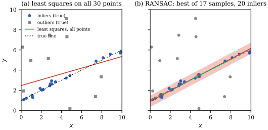
A line through 20 inliers on $y = 0.5x + 1$ plus 10 outliers (seed 9517). (a) Least squares on all 30 points gives $y = 0.288x + 2.472$, slope off by 42%. (b) RANSAC, best of 17 two-point samples (circled): its band of half-width $\delta = 0.5$ holds exactly the 20 true inliers, and the refit on them (dashed) is $y = 0.502x + 1.029$.

how many iterations

Proposition (RANSAC iteration count)

If a fraction $\rho$ of the data are inliers, then $N$ samples of size $s$ include at least one all-inlier sample with probability at least $p$ when \[ N \ge \frac{\log(1-p)}{\log(1-\rho^s)} . \]

At $p = 0.99$:

model	$s$	$\rho = 0.5$	$\rho = 0.8$
translation	1	7	3
line	2	17	5
affine	3	35	7
homography	4	72	9

$N$ grows like $\rho^{-s}$, which is why the sample is always the minimal one. A homography at $\rho = 0.1$ needs about 46,000 iterations.

proofs

Proof (RANSAC iteration count)

One sample. All $s$ data are inliers with probability $\rho^s$ (exactly, drawing with replacement; nearly, without, when there are many data).

All $N$ samples fail. The draws are independent, so this has probability $(1-\rho^s)^N$.

Require success with probability $p$. We need $(1-\rho^s)^N \le 1-p$. Take logarithms; both $\log(1-\rho^s)$ and $\log(1-p)$ are negative, so dividing flips the inequality and gives $N \ge \log(1-p)/\log(1-\rho^s)$.

when RANSAC fails, and what to use instead

Low inlier ratio. The $\rho^{-s}$ blow-up makes RANSAC impractical below roughly 10–20% inliers for a homography. Better matching (a stricter ratio, cross-checking both directions) or guided sampling (PROSAC, which tries the best-scoring matches first) helps.
Wrong $\delta$. Too small and true inliers are rejected; too large and outliers vote. Set it from the expected localisation noise, a few pixels for SIFT keypoints.
Two structures. With two planes or two independently moving objects RANSAC returns only the one with more support; sequential RANSAC (fit, remove inliers, repeat) or multi-model methods find the rest.

Use RANSAC whenever the correspondences contain gross errors, as every ratio-tested match set does. Plain least squares is right only when every correspondence is known to be correct, and it remains the final refit on the inliers.

stitching two views of the castle

Now everything joins up.

Definition (Algorithm: two-view stitching)

Detect SIFT keypoints and descriptors in both images.
For each descriptor in image 1 find its 2 nearest neighbours in image 2 and keep the match if it passes the ratio test.
Fit a homography to the surviving matches by RANSAC, then refine it by least squares on the inliers.
Warp image 1 into image 2’s frame on a canvas large enough for both, and blend.

Example (A panorama from two views of the castle)

The course did this on its own pair of photographs. Here the second view is manufactured, so the true answer is known. View 1 is the left $330\times430$ part of the Lab 1 castle image. View 2 is the whole image rotated by $12^\circ$, scaled by 1.1 and given a perspective term, then cropped to $330\times430$ so that 55% of view 1 appears in it; both views get Gaussian noise of standard deviation 3 grey levels (seed 9517). Brute-force matching with $k = 2$ and ratio 0.75; OpenCV’s findHomography with RANSAC and $\delta = 5$ pixels.

541 matches pass the ratio test, and RANSAC keeps 521 of them (96%) as inliers. They are exactly the 521 matches the true homography calls correct: no false match kept, no true one lost. At $\rho = 0.96$ a homography needs only 3 iterations for 99% confidence.
The true homography and the RANSAC estimate, scaled to $h_{33} = 1$, are \[ \mathbf H_{\text{true}} \approx \begin{pmatrix} 0.968 & 0.240 & -178.7 \\ -0.298 & 1.057 & 51.9 \\ -0.0004 & 0.0002 & 1 \end{pmatrix}, \qquad \mathbf H \approx \begin{pmatrix} 0.967 & 0.240 & -178.7 \\ -0.298 & 1.057 & 51.9 \\ -0.0004 & 0.0002 & 1 \end{pmatrix} . \] The non-zero $h_{31}, h_{32}$ are the perspective part, put there on purpose. Over every pixel of the overlap, $\mathbf H$ sends points within 0.16 pixels of where $\mathbf H_{\text{true}}$ sends them (mean 0.10).
The payoff. On the 521 inliers the median reprojection error is 0.18 pixels with this $\mathbf H$. A homography fitted to all 541 matches without RANSAC misses the same points by a median 5.60 pixels, and is off from $\mathbf H_{\text{true}}$ by 8.1 pixels on average and 29 at worst: 20 false matches, under 4% of the data, are enough to wreck the plain fit.
View 1’s corners land at $(-179,52)$, $(161,-53)$, $(255,427)$, $(-70,468)$, so a canvas of $509\times522$ pixels holds both views, and view 2 is pasted on top.

The warped outline of view 1 is a general quadrilateral, not a parallelogram. An affine model could not have aligned these views.

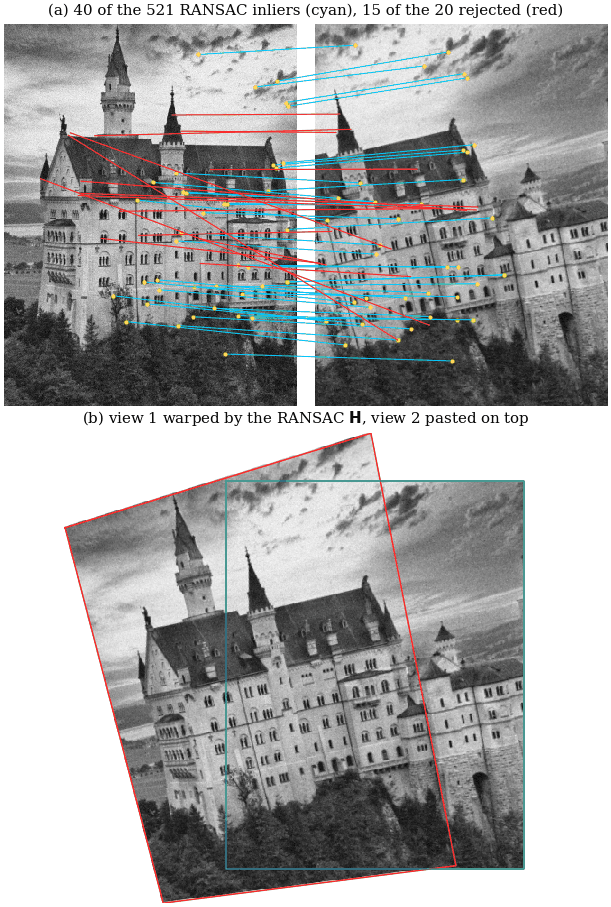
(a) SIFT matches between two castle views (view 2 is the castle under a known homography, with noise): 40 of the 521 RANSAC inliers (cyan) and 15 of the 20 rejected matches (red). The red lines cross the castle at angles no single transformation could produce. (b) View 1 warped by the RANSAC homography (red outline) with view 2 pasted on top (green outline); no blending.

where stitching breaks

The seam in panel (b) is almost invisible only because view 2 was made from view 1’s pixels: same exposure, and a relation that is exactly a homography. Real photographs differ in exposure, and with nothing blended the seam shows; real stitchers feather or multi-band blend across the overlap and pick seams through low-contrast regions. Parallax is the deeper limit. A homography is exact only for a planar scene or a purely rotating camera. Walk sideways between shots and near objects (a lamp post, the trees in front of a building) shift relative to far ones, no single $\mathbf H$ fits both, and the result ghosts. For many images, pairwise homographies accumulate drift around the panorama; bundle adjustment fixes it by refining all camera rotations jointly.

summary

step	tool	key knob
detect	DoG extrema, 26 nbrs	contrast thresh.
describe	4x4x8 gradient hists	clip at 0.2
match	NN + ratio test	ratio 0.75 to 0.8
align	homography by RANSAC	$\delta$, $N$

Further reading: Szeliski, Computer Vision: Algorithms and Applications, 2nd ed., §7.1 (feature detection, description and matching) and §8.1–8.2 (feature-based alignment and image stitching).

SIFT, Matching and Stitching