Icons
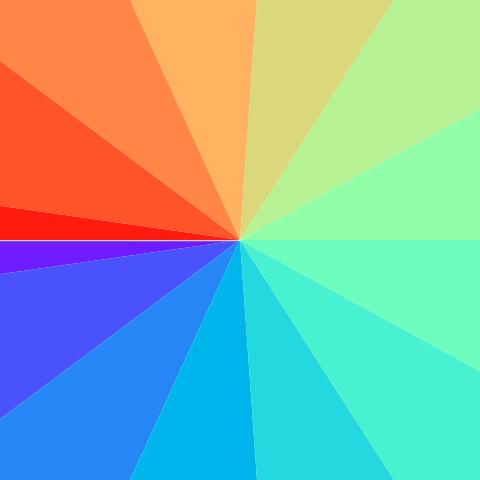
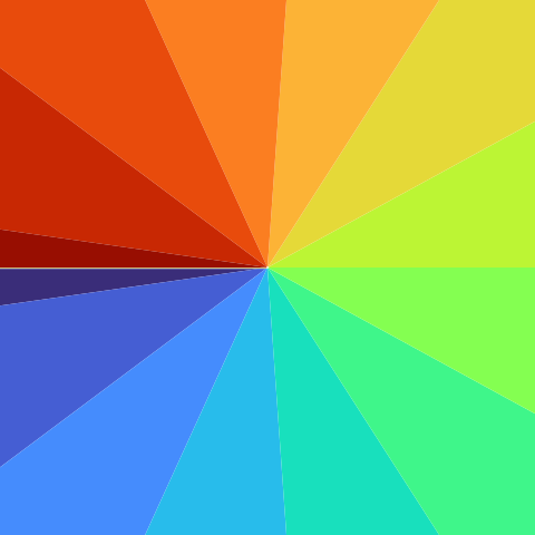
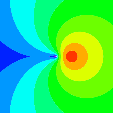
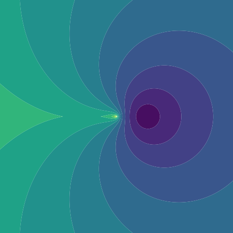
All of the site favicons that I use have been generated by contour plots of the complex logarithm and complex exponential functions.
Experiments
HSV | Viridis | Cividis | Inferno | Jet | Magma | Plasma | Rainbow | Turbo
Real
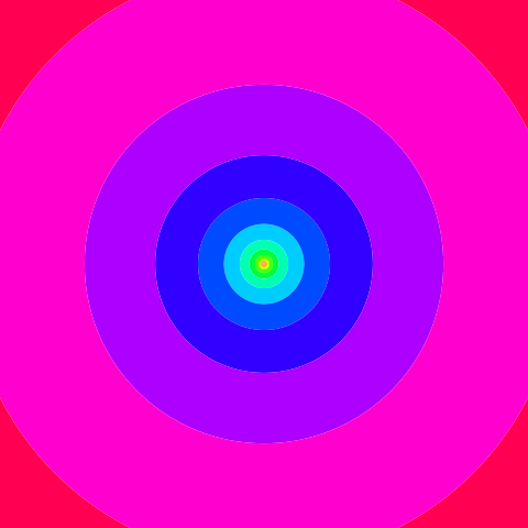
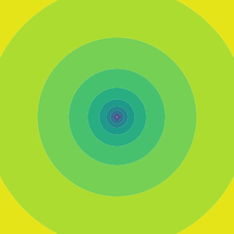
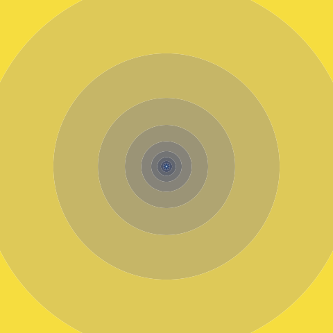
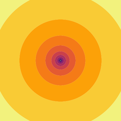
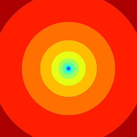
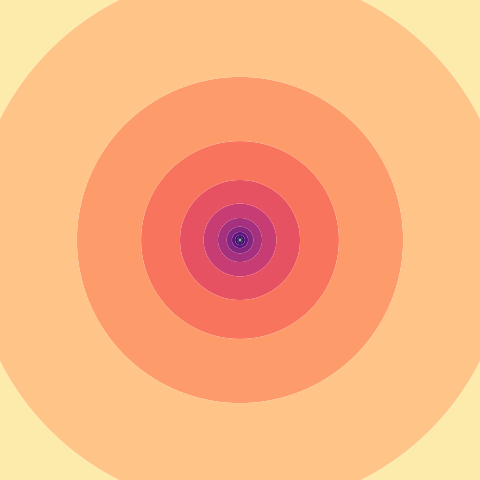
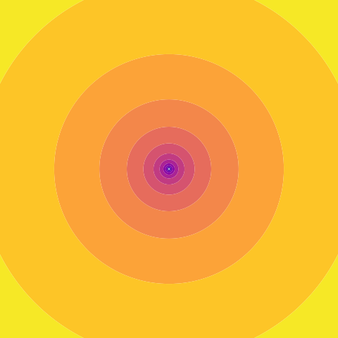
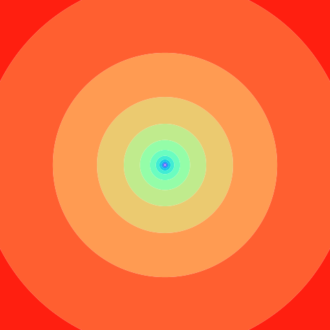
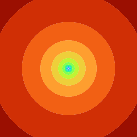
Imaginary
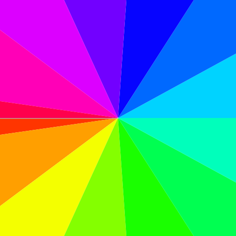
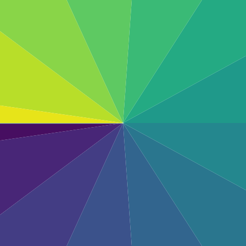
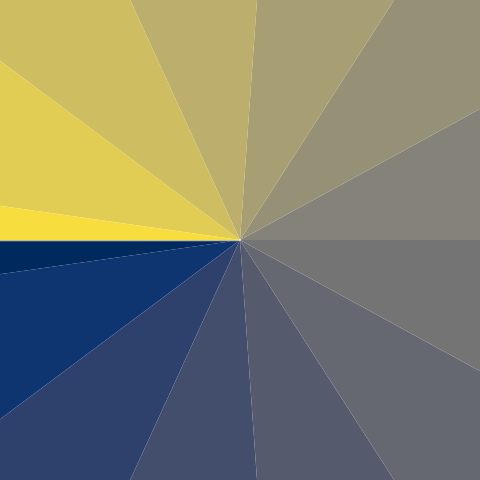
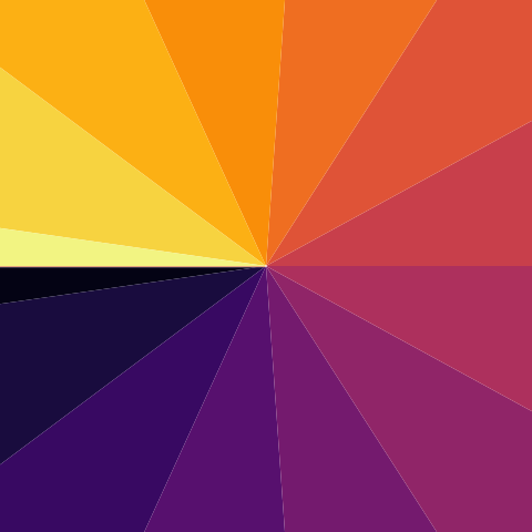
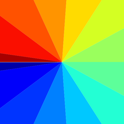
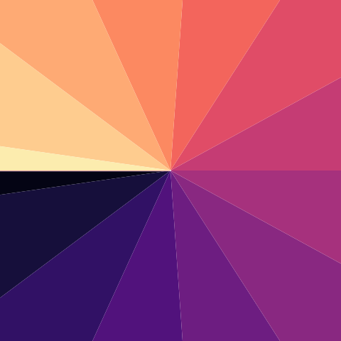
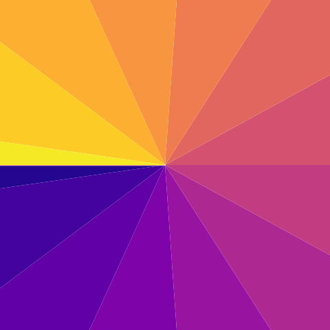
Absolute
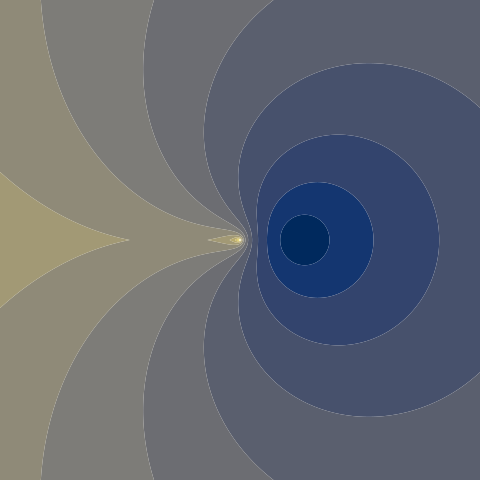
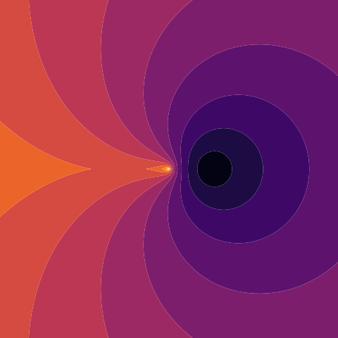
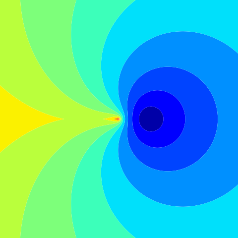
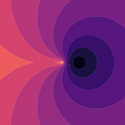
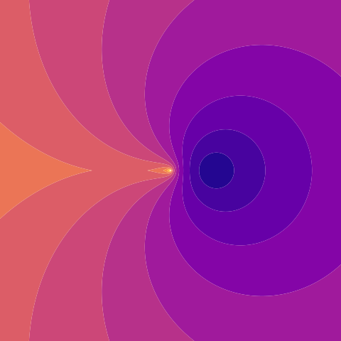
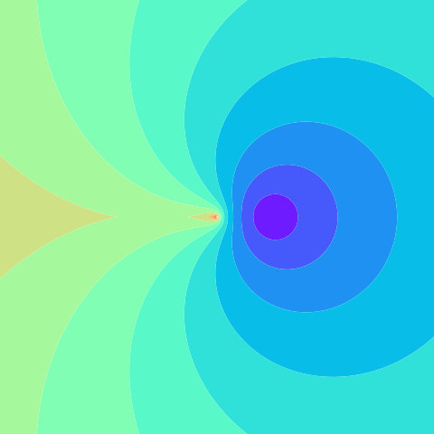
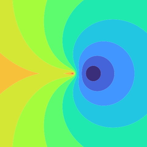
HSV | Viridis | Cividis | Inferno | Jet | Magma | Plasma | Rainbow | Turbo
Real
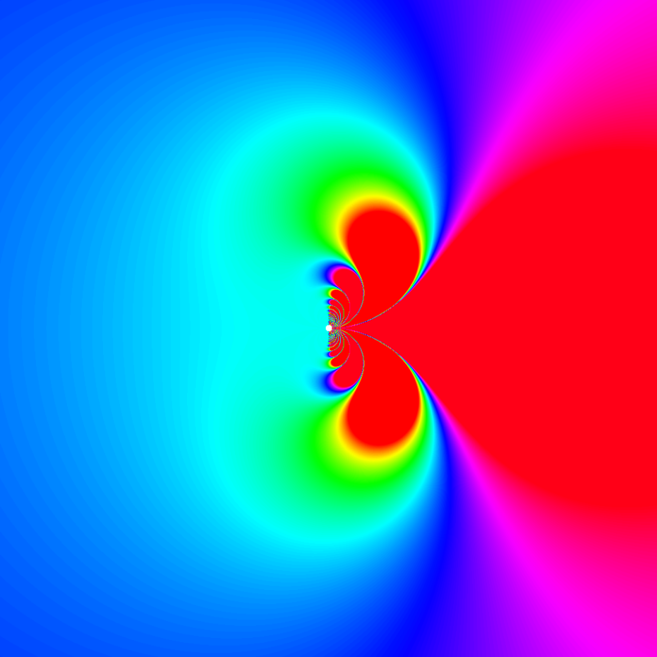
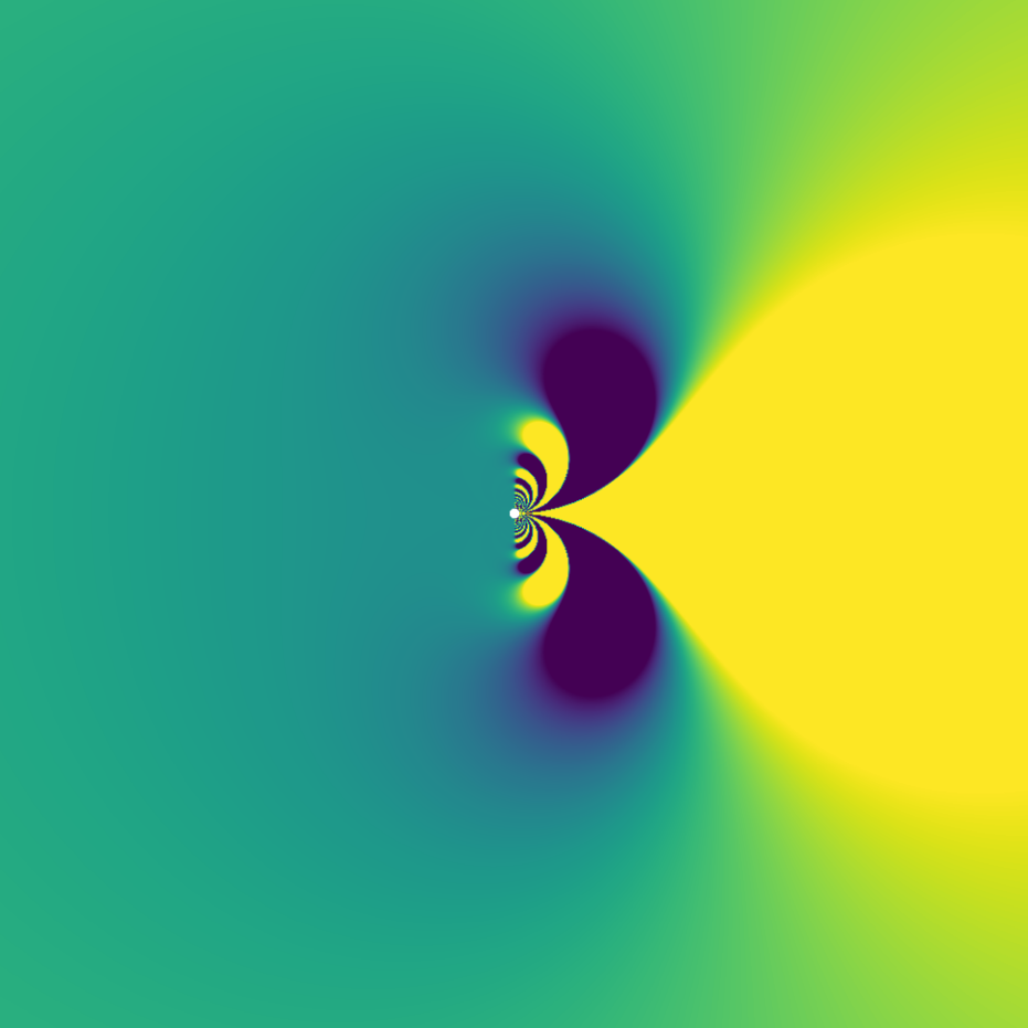
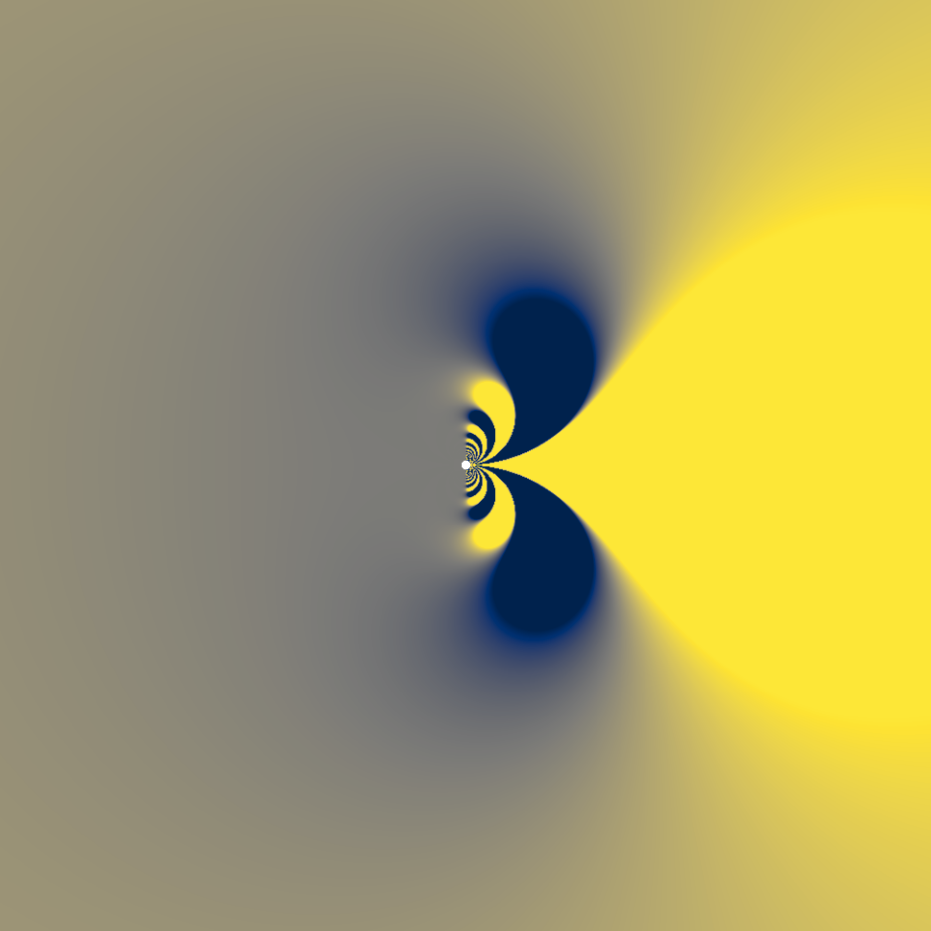
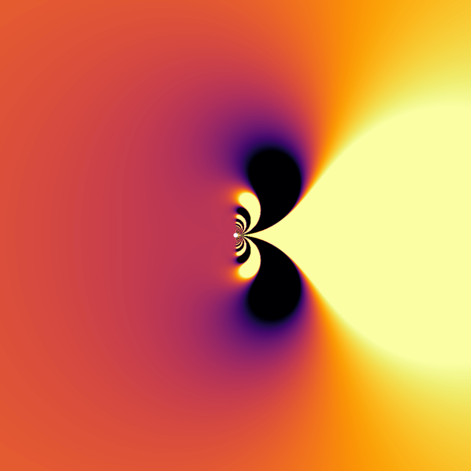
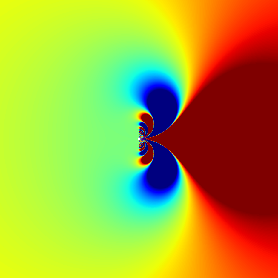
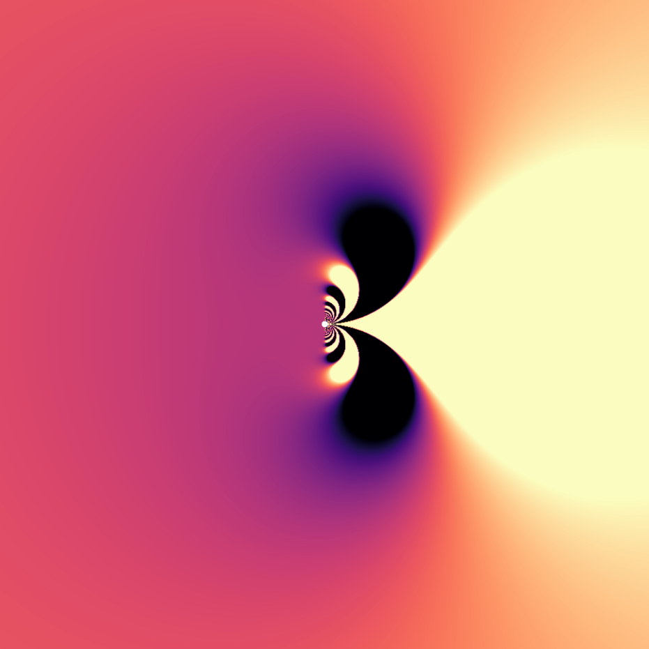
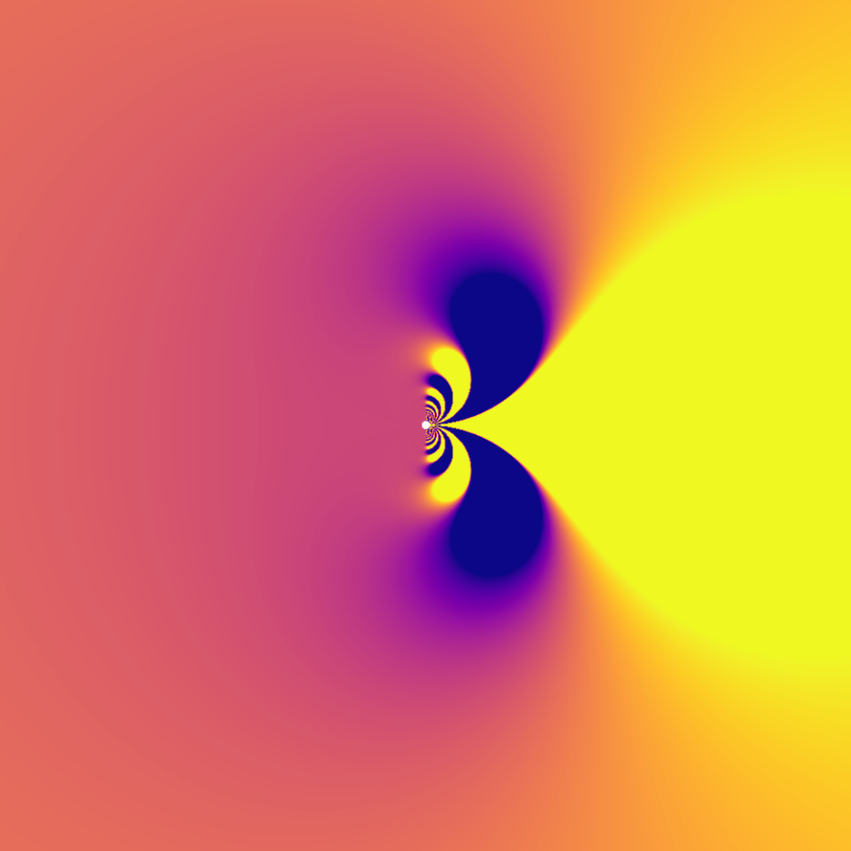
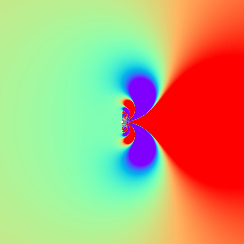
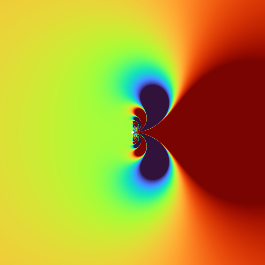
Imaginary
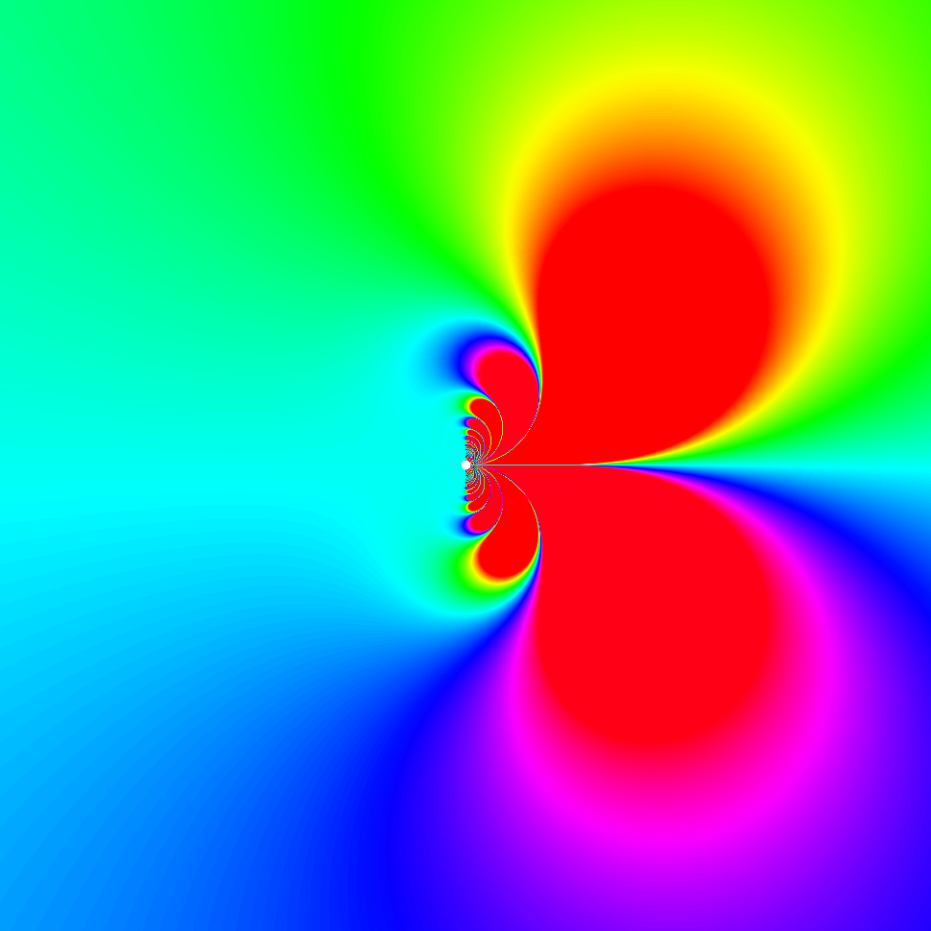
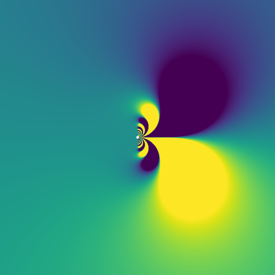
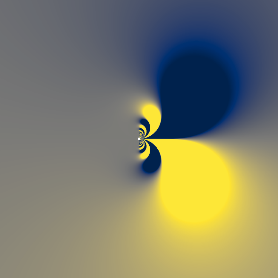
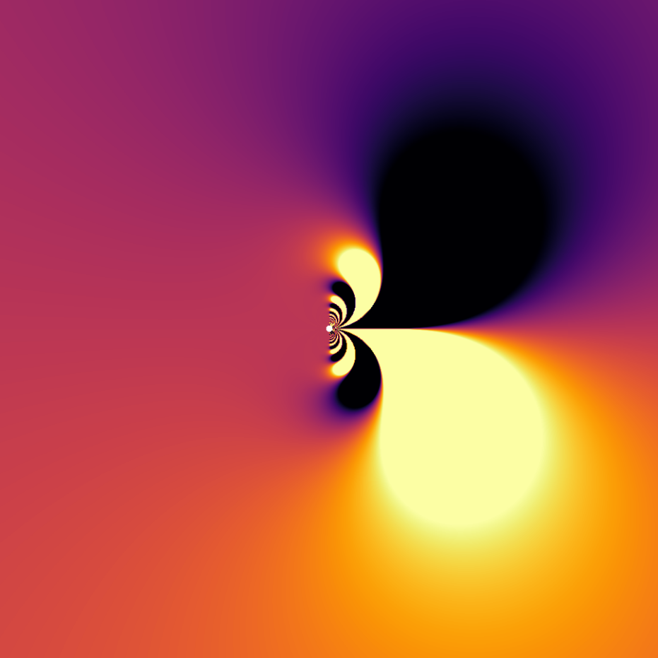
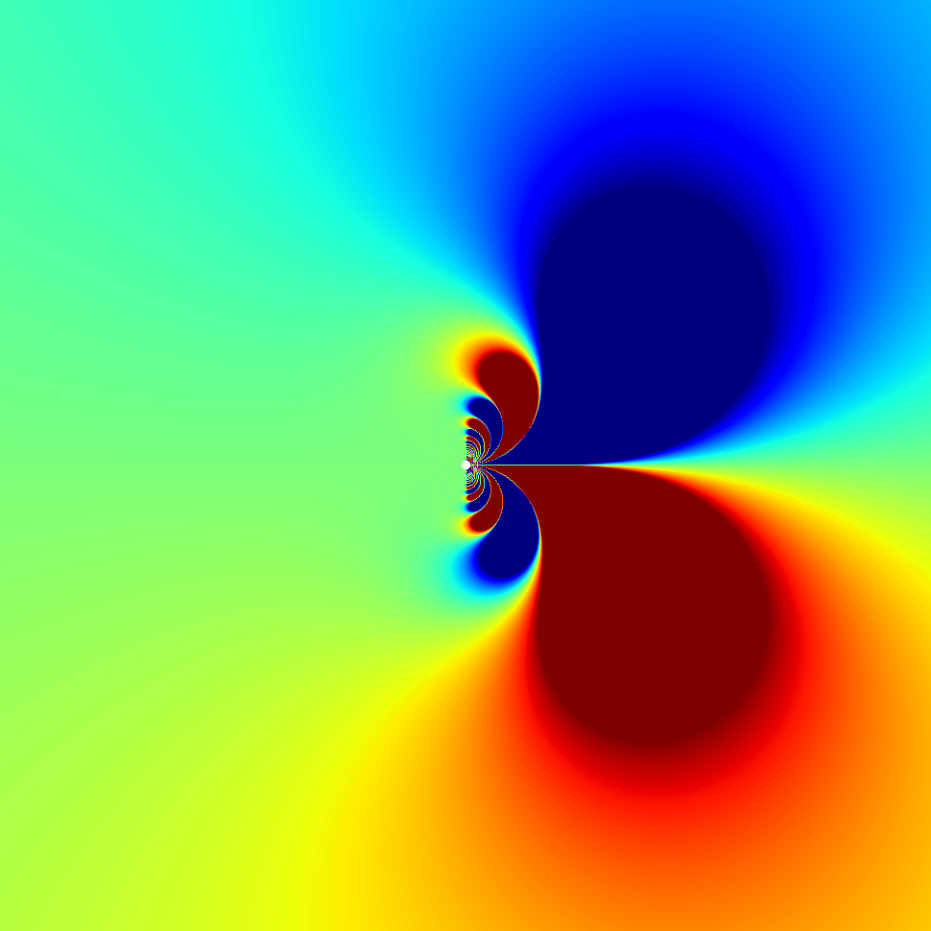
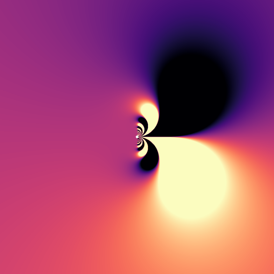
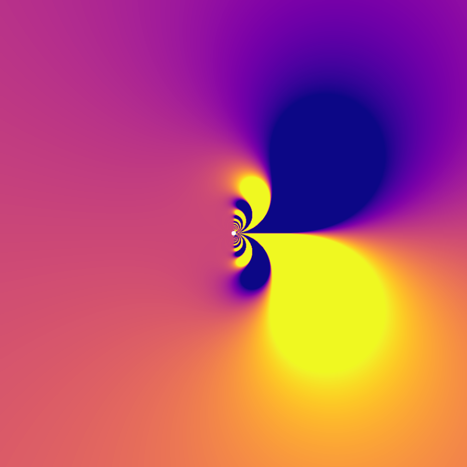
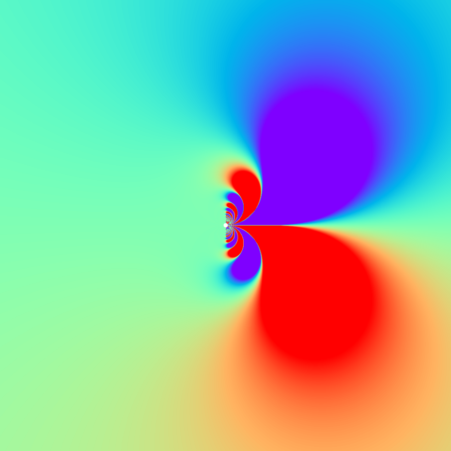
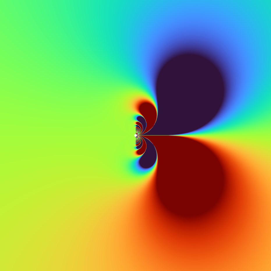
Absolute
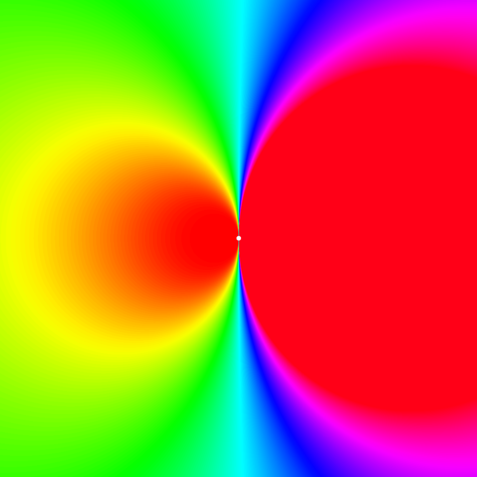
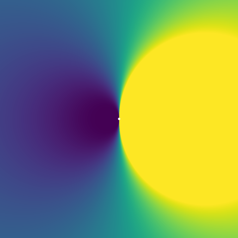
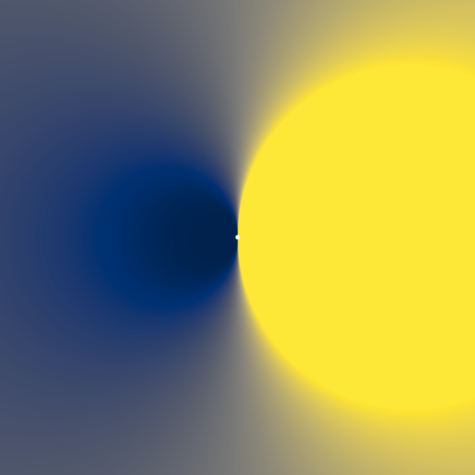
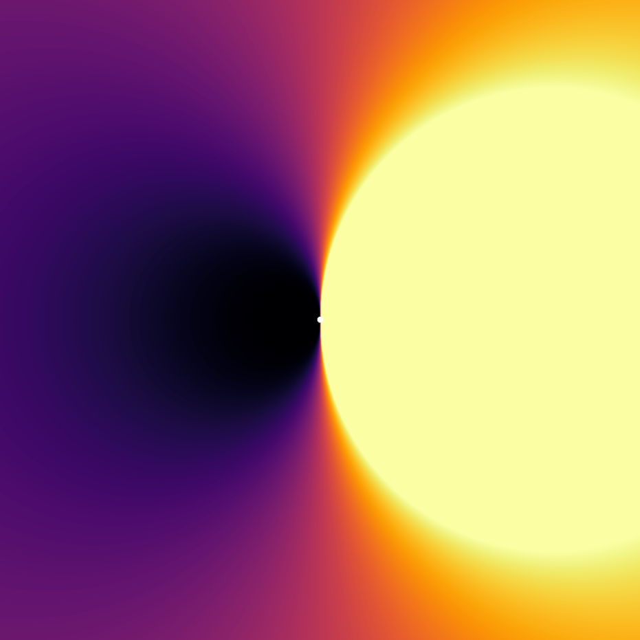
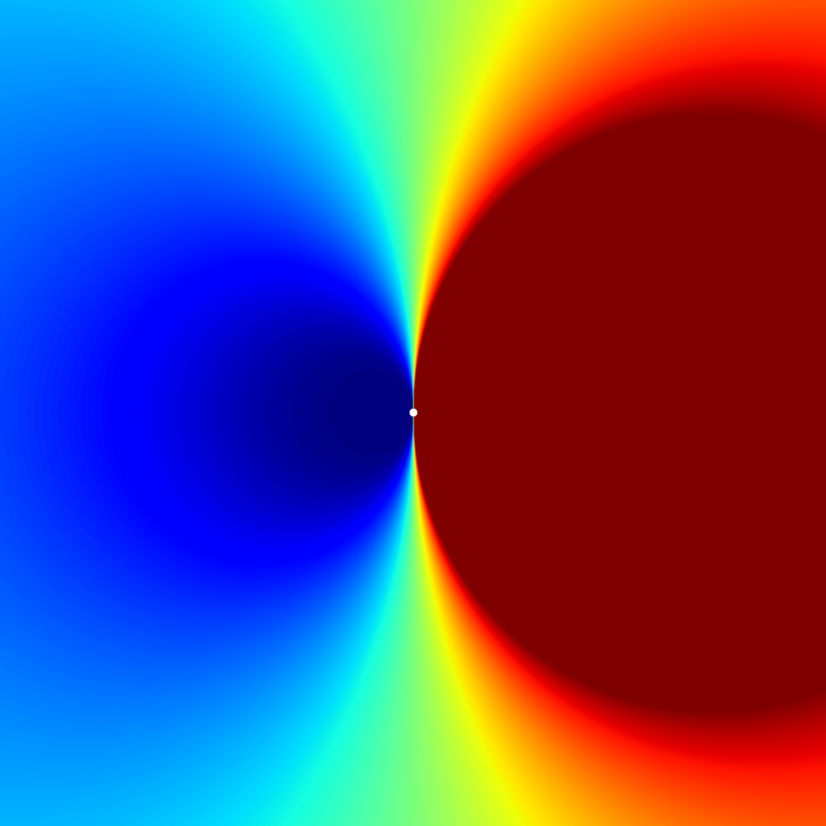
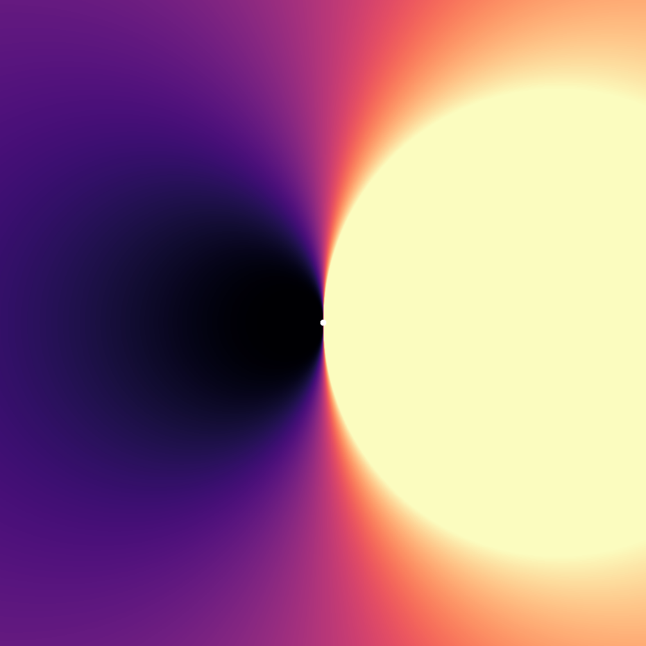
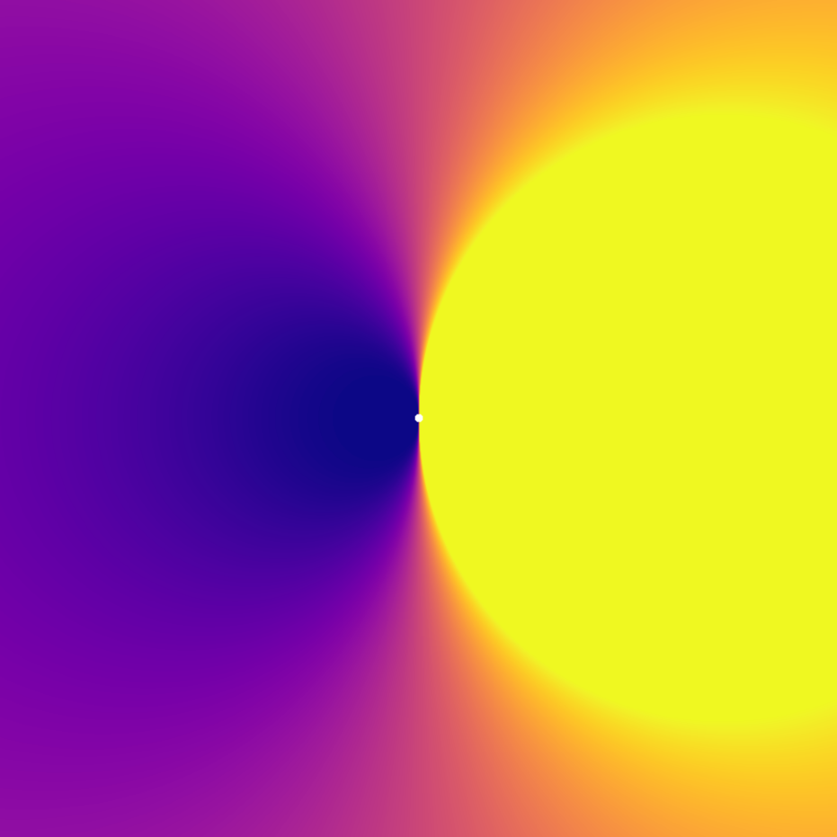
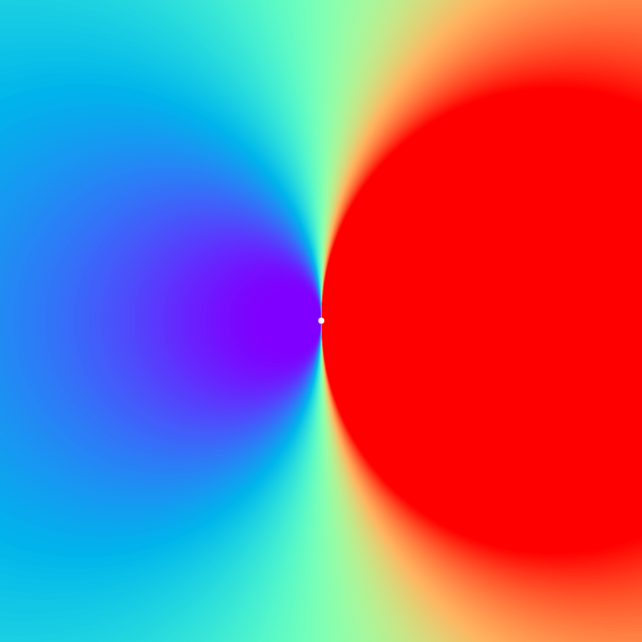
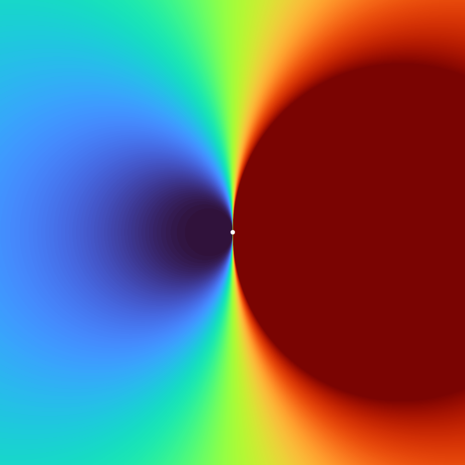
Mathematics
Wolfram Alpha does a better job regarding this than I can. I do not understand the behaviour of these functions, especially at the branch points:
https://functions.wolfram.com/ElementaryFunctions/Log/visualizations/5/
https://functions.wolfram.com/ElementaryFunctions/Exp/visualizations/5/
Code
GPT o1 model produced these figures for me, here are the included code-blocks that have been version controlled as part of a larger icons repository.
#!/usr/bin/env python3
"""
Generate three separate SVG images:
1) Re[ln(x + i y)]
2) Im[ln(x + i y)]
3) |ln(x + i y)|

All plotted over x,y in [-4,4], with discrete color bands.

Usage:
  python plot_ln_complex.py [--cmap CMAP]

Example:
  python plot_ln_complex.py --cmap rainbow

This will produce:
  real_part.svg,
  imag_part.svg,
  abs_part.svg
"""

import numpy as np
import matplotlib.pyplot as plt
import argparse

def main():
    # A list of common matplotlib colormaps you might try for discrete color blocks
    all_cmaps = [
        'rainbow', 'hsv', 'jet', 'plasma', 'inferno', 'magma',
        'cividis', 'viridis', 'turbo'
    ]

    parser = argparse.ArgumentParser(
        description="Generate discrete color-band plots for Re, Im, and |ln(x + i y)| over [-4,4]x[-4,4]."
    )
    parser.add_argument(
        '--cmap',
        type=str,
        default='rainbow',
        help=(
            "Colormap to use. Some options include:\n"
            f"{', '.join(all_cmaps)}\n"
            "For more, see: https://matplotlib.org/stable/tutorials/colors/colormaps.html"
        )
    )
    args = parser.parse_args()

    # ---------------------------------------------------
    # Domain: x,y in [-4,4]
    # We'll include 401 points per axis so that 0 is included.
    # ---------------------------------------------------
    n_points = 401
    x_vals = np.linspace(-4, 4, n_points)
    y_vals = np.linspace(-4, 4, n_points)
    X, Y = np.meshgrid(x_vals, y_vals)

    # Avoid log(0) by masking out the point z=0
    Z = X + 1j * Y
    zero_mask = (X == 0) & (Y == 0)
    Z[zero_mask] = np.nan

    # Compute principal branch of the complex log
    with np.errstate(divide='ignore', invalid='ignore'):
        Z_ln = np.log(Z)

    # Extract real part, imaginary part, and magnitude
    ln_real = np.real(Z_ln)
    ln_imag = np.imag(Z_ln)
    ln_abs  = np.abs(Z_ln)

    # Decide how many discrete levels to use
    n_levels = 12  # Adjust if you want more or fewer color bands

    # ---------------------------------------------------
    # 1) Real part of ln(z)
    # ---------------------------------------------------
    fig_re, ax_re = plt.subplots(figsize=(6, 5), dpi=100)
    cs_re = ax_re.contourf(
        X, Y, ln_real,
        levels=n_levels,
        cmap=args.cmap
    )
    ax_re.set_aspect('equal', 'box')
    ax_re.axis('off')
    plt.subplots_adjust(left=0, right=1, top=1, bottom=0)
    fig_re.savefig("real_part.svg", format="svg", bbox_inches='tight', pad_inches=0)
    plt.close(fig_re)

    # ---------------------------------------------------
    # 2) Imag part of ln(z)
    # ---------------------------------------------------
    fig_im, ax_im = plt.subplots(figsize=(6, 5), dpi=100)
    cs_im = ax_im.contourf(
        X, Y, ln_imag,
        levels=n_levels,
        cmap=args.cmap
    )
    ax_im.set_aspect('equal', 'box')
    ax_im.axis('off')
    plt.subplots_adjust(left=0, right=1, top=1, bottom=0)
    fig_im.savefig("imag_part.svg", format="svg", bbox_inches='tight', pad_inches=0)
    plt.close(fig_im)

    # ---------------------------------------------------
    # 3) Absolute value of ln(z)
    # ---------------------------------------------------
    fig_abs, ax_abs = plt.subplots(figsize=(6, 5), dpi=100)
    cs_abs = ax_abs.contourf(
        X, Y, ln_abs,
        levels=n_levels,
        cmap=args.cmap
    )
    ax_abs.set_aspect('equal', 'box')
    ax_abs.axis('off')
    plt.subplots_adjust(left=0, right=1, top=1, bottom=0)
    fig_abs.savefig("abs_part.svg", format="svg", bbox_inches='tight', pad_inches=0)
    plt.close(fig_abs)


if __name__ == "__main__":
    main()
import numpy as np
import matplotlib
matplotlib.use('Agg')  # Use non-interactive backend
import matplotlib.pyplot as plt
import argparse
import os

def get_available_colormaps():
    """Returns a list of all available colormaps in matplotlib."""
    return plt.colormaps()

def exp_inv_complex(Z):
    """Compute exp(1/z) for a complex array Z."""
    with np.errstate(divide='ignore', invalid='ignore'):
        return np.exp(1 / Z)

def plot_complex_exp(cmap='RdYlBu_r', output_file=None, resolution=1001, singularity_size=0.01):
    """
    Plot the real component of exp(1/z) using the specified colormap.

    Args:
        cmap (str): Name of the matplotlib colormap to use.
                   Must be one of the available matplotlib colormaps.
        output_file (str, optional): Path to save the SVG file.
                                   If None, displays the plot instead.
        resolution (int): Number of points in each dimension. Higher values give better detail.
        singularity_size (float): Radius around z=0 to mask for the singularity.
    """
    # Generate grid points with high resolution
    x_vals = np.linspace(-1, 1, resolution)
    y_vals = np.linspace(-1, 1, resolution)
    X, Y = np.meshgrid(x_vals, y_vals)

    # Create complex grid Z = X + iY with smaller singularity
    Z = X + 1j * Y
    Z[np.abs(Z) < singularity_size] = np.nan

    # Compute exp(1/Z)
    W = exp_inv_complex(Z)
    real_part = np.real(W)
    real_part = np.clip(real_part, -2, 2)

    # Create minimal plot
    fig = plt.figure(figsize=(10, 10))
    ax = fig.add_subplot(111)
    im = ax.imshow(
        real_part,
        extent=[-1, 1, -1, 1],
        cmap=cmap,
        origin='lower',
        aspect='equal',
        interpolation='bilinear'
    )

    # Remove all decorations
    ax.set_xticks([])
    ax.set_yticks([])
    ax.set_frame_on(False)

    plt.tight_layout()

    if output_file:
        # Ensure the output directory exists
        os.makedirs(os.path.dirname(output_file) if os.path.dirname(output_file) else '.', exist_ok=True)
        plt.savefig(output_file, format='svg', bbox_inches='tight', pad_inches=0)
        plt.close()
    else:
        plt.show()

def plot_imaginary_exp(cmap='RdYlBu_r', output_file=None, resolution=1001, singularity_size=0.01):
    """
    Plot the imaginary component of exp(1/z) using the specified colormap.

    Args:
        cmap (str): Name of the matplotlib colormap to use.
                   Must be one of the available matplotlib colormaps.
        output_file (str, optional): Path to save the SVG file.
                                   If None, displays the plot instead.
        resolution (int): Number of points in each dimension. Higher values give better detail.
        singularity_size (float): Radius around z=0 to mask for the singularity.
    """
    # Generate grid points with high resolution
    x_vals = np.linspace(-1, 1, resolution)
    y_vals = np.linspace(-1, 1, resolution)
    X, Y = np.meshgrid(x_vals, y_vals)

    # Create complex grid Z = X + iY with smaller singularity
    Z = X + 1j * Y
    Z[np.abs(Z) < singularity_size] = np.nan

    # Compute exp(1/Z)
    W = exp_inv_complex(Z)
    imag_part = np.imag(W)
    imag_part = np.clip(imag_part, -2, 2)

    # Create minimal plot
    fig = plt.figure(figsize=(10, 10))
    ax = fig.add_subplot(111)
    im = ax.imshow(
        imag_part,
        extent=[-1, 1, -1, 1],
        cmap=cmap,
        origin='lower',
        aspect='equal',
        interpolation='bilinear'
    )

    # Remove all decorations
    ax.set_xticks([])
    ax.set_yticks([])
    ax.set_frame_on(False)

    plt.tight_layout()

    if output_file:
        # Ensure the output directory exists
        os.makedirs(os.path.dirname(output_file) if os.path.dirname(output_file) else '.', exist_ok=True)
        plt.savefig(output_file, format='svg', bbox_inches='tight', pad_inches=0)
        plt.close()
    else:
        plt.show()

def plot_absolute_exp(cmap='hsv', output_file=None, resolution=1001, singularity_size=0.01):
    """
    Plot the absolute value of exp(1/z) using the specified colormap.
    The color represents the argument (phase) of the complex number.

    Args:
        cmap (str): Name of the matplotlib colormap to use.
                   Must be one of the available matplotlib colormaps.
        output_file (str, optional): Path to save the SVG file.
                                   If None, displays the plot instead.
        resolution (int): Number of points in each dimension. Higher values give better detail.
        singularity_size (float): Radius around z=0 to mask for the singularity.
    """
    # Generate grid points with high resolution
    x_vals = np.linspace(-1, 1, resolution)
    y_vals = np.linspace(-1, 1, resolution)
    X, Y = np.meshgrid(x_vals, y_vals)

    # Create complex grid Z = X + iY with smaller singularity
    Z = X + 1j * Y
    Z[np.abs(Z) < singularity_size] = np.nan

    # Compute exp(1/Z)
    W = exp_inv_complex(Z)
    abs_val = np.abs(W)
    arg_val = np.angle(W, deg=True)

    # Normalize absolute value for better visualization
    abs_val = np.clip(abs_val, 0, 2)

    # Create minimal plot
    fig = plt.figure(figsize=(10, 10))
    ax = fig.add_subplot(111)

    # Plot the absolute value with phase coloring
    im = ax.imshow(
        abs_val,  # Use absolute value for the data
        extent=[-1, 1, -1, 1],
        cmap=cmap,
        origin='lower',
        aspect='equal',
        interpolation='bilinear'
    )

    # Remove all decorations
    ax.set_xticks([])
    ax.set_yticks([])
    ax.set_frame_on(False)

    plt.tight_layout()

    if output_file:
        # Ensure the output directory exists
        os.makedirs(os.path.dirname(output_file) if os.path.dirname(output_file) else '.', exist_ok=True)
        plt.savefig(output_file, format='svg', bbox_inches='tight', pad_inches=0)
        plt.close()
    else:
        plt.show()

def main():
    """Main function to handle command line arguments and create the plots."""
    parser = argparse.ArgumentParser(
        description='Visualize various components of exp(1/z) with customizable colormap.',
        formatter_class=argparse.ArgumentDefaultsHelpFormatter
    )

    parser.add_argument(
        '--cmap',
        type=str,
        default='RdYlBu_r',
        choices=get_available_colormaps(),
        help='Matplotlib colormap to use for visualization'
    )

    parser.add_argument(
        '--output-prefix',
        type=str,
        default=None,
        help='Prefix for output SVG files. If not provided, displays the plots instead.'
    )

    parser.add_argument(
        '--resolution',
        type=int,
        default=1001,
        help='Number of points in each dimension. Higher values give better detail.'
    )

    parser.add_argument(
        '--singularity-size',
        type=float,
        default=0.01,
        help='Radius around z=0 to mask for the singularity.'
    )

    args = parser.parse_args()

    # Generate all three visualizations
    if args.output_prefix:
        real_output = f"{args.output_prefix}_real.svg"
        imag_output = f"{args.output_prefix}_imag.svg"
        abs_output = f"{args.output_prefix}_abs.svg"
    else:
        real_output = None
        imag_output = None
        abs_output = None

    # Plot real part
    plot_complex_exp(args.cmap, real_output, args.resolution, args.singularity_size)

    # Plot imaginary part
    plot_imaginary_exp(args.cmap, imag_output, args.resolution, args.singularity_size)

    # Plot absolute value with the same colormap as the others
    plot_absolute_exp(args.cmap, abs_output, args.resolution, args.singularity_size)

if __name__ == '__main__':
    main()
Final Orbs
There has been a degree of iteration across functions and heatmaps, but ultimately here are the 5 plots that I have settled on for my 5 products; abaj.ai, bots.abaj.ai, games.abaj.ai, trades.abaj.ai, tools.abaj.ai.

absolute hsv
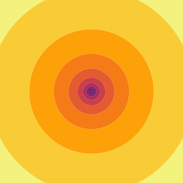
real inferno

imaginary jet
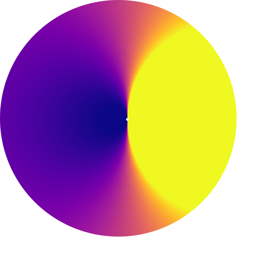
absolute plasma
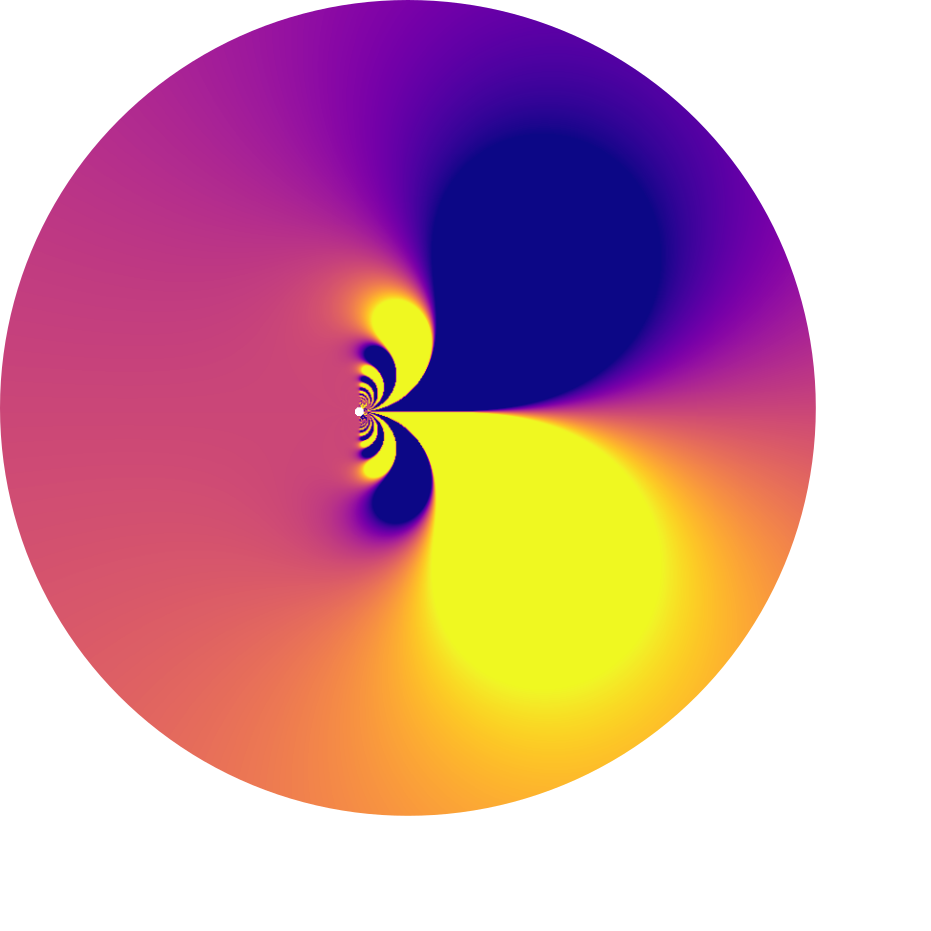
imaginary plasma
The Bazaar Orb
The sixth orb breaks the complex-function tradition on purpose: the bazaar is a storefront, not a maths property, so its orb is a dynamical system instead of a contour plot — a milky-marble sphere whose golden streamlines are RK4-integrated trajectories of a two-vortex flow (a spiral sink at the origin plus a soft off-centre vortex). Every trajectory tapers and brightens as it falls inward, and the site’s curved diamond ✦ sits at the sink where all influence collects. The marble ground is domain-warped fBm veining; the matte finish is limb darkening plus a broad diffuse key light — deliberately no specular highlight.
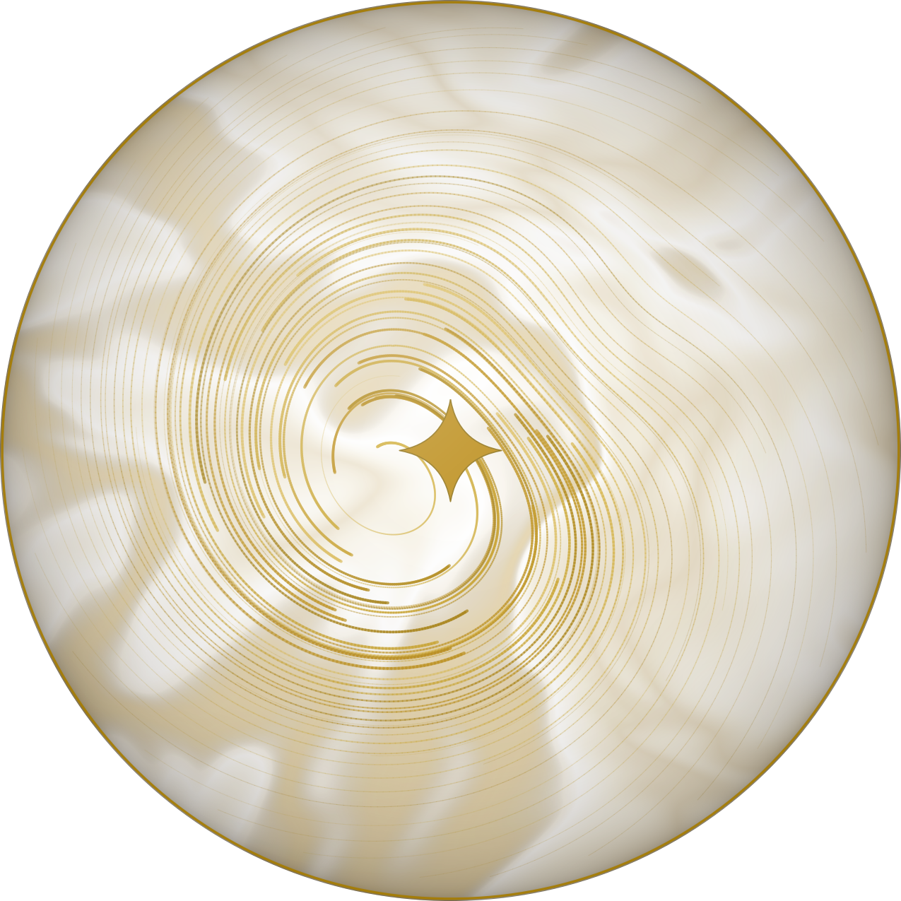
milky-marble golden flow — bazaar.abaj.ai
The generator is version-controlled with the other icons:
#!/usr/bin/env python3
"""bazaar.abaj.ai orb — milky-marble ground, golden dynamical-system flow, matte shading.

Family style of the sibling icons (matplotlib figure clipped to a circle, 612pt).
A damped two-vortex flow is integrated by hand (RK4) so line density stays airy;
trajectories are drawn as tapering gold strokes over marble veining, then a
radial matte falloff turns the disc into an orb.
"""

import numpy as np
import matplotlib

matplotlib.use('Agg')
import matplotlib.pyplot as plt
from matplotlib.collections import LineCollection
from matplotlib.colors import LinearSegmentedColormap, to_rgb

rng = np.random.default_rng(7)

IVORY = '#fdfbf4'
GOLDS = ['#8a6a08', '#a67c00', '#b8860b', '#c9a227', '#d4af37', '#e0c268']

# ── marble ground: domain-warped fBm veins ─────────────────────────────────
N = 900
lin = np.linspace(-3, 3, N)
X, Y = np.meshgrid(lin, lin)


def fbm(x, y, octaves=5, seed=0):
    r = np.random.default_rng(seed)
    v = np.zeros_like(x)
    amp, freq = 1.0, 0.55
    for _ in range(octaves):
        px, py = r.uniform(0, 100, 2)
        v += amp * np.sin(freq * (x + px) + 1.7 * np.cos(freq * (y + py)))
        v += amp * np.cos(freq * (y + py) - 1.3 * np.sin(freq * (x + px) * 0.7))
        amp *= 0.55
        freq *= 1.9
    return v


warp = fbm(X, Y, 4, seed=11)
veins = fbm(X + 0.4 * warp, Y + 0.4 * warp, 5, seed=23)
marble = np.abs(np.sin(1.1 * veins))
marble_cmap = LinearSegmentedColormap.from_list(
    'marble', [(0.0, '#ece2cc'), (0.45, '#f8f4e8'), (0.8, '#ffffff'), (1.0, '#efe6d2')]
)

# ── the dynamical system: spiral sink + off-centre secondary vortex ────────
def flow(x, y):
    # primary: gentle spiral sink at origin (no limit cycle → no pile-up)
    u = -y - 0.16 * x
    v = x - 0.16 * y
    # secondary influence: soft vortex up-right
    dx, dy = x - 1.15, y - 0.85
    d2 = dx * dx + dy * dy + 0.4
    u += 0.9 * dy / d2
    v += -0.9 * dx / d2
    return u, v


def rk4_path(p, h=0.02, steps=340):
    pts = [p]
    x, y = p
    for _ in range(steps):
        k1 = flow(x, y)
        k2 = flow(x + h / 2 * k1[0], y + h / 2 * k1[1])
        k3 = flow(x + h / 2 * k2[0], y + h / 2 * k2[1])
        k4 = flow(x + h * k3[0], y + h * k3[1])
        x += h / 6 * (k1[0] + 2 * k2[0] + 2 * k3[0] + k4[0])
        y += h / 6 * (k1[1] + 2 * k2[1] + 2 * k3[1] + k4[1])
        pts.append((x, y))
        if x * x + y * y < 0.004:
            break
    return np.array(pts)


# ── figure ─────────────────────────────────────────────────────────────────
fig = plt.figure(figsize=(8.5, 8.5), dpi=72)  # 612pt like the siblings
ax = fig.add_axes([0, 0, 1, 1])
ax.set_xlim(-3, 3)
ax.set_ylim(-3, 3)
ax.set_aspect('equal')
ax.axis('off')

def clipped(artist):
    artist.set_clip_path(plt.Circle((0, 0), 3.0, transform=ax.transData))
    return artist

# marble ground
clipped(ax.imshow(marble, extent=[-3, 3, -3, 3], cmap=marble_cmap,
                  origin='lower', interpolation='bilinear', zorder=0))

# faint gold veining on the strongest ridges
vein = np.where(marble > 0.88, marble, np.nan)
clipped(ax.imshow(vein, extent=[-3, 3, -3, 3], origin='lower',
                  cmap=LinearSegmentedColormap.from_list('gv', ['#00000000', '#b8860b30']),
                  interpolation='bilinear', zorder=1))

# ── golden trajectories: two rings of seeds + a few strays ─────────────────
seeds = []
for r, n, jit in [(2.85, 26, 0.05), (2.1, 14, 0.12)]:
    for th in np.linspace(0, 2 * np.pi, n, endpoint=False):
        th2 = th + rng.uniform(-jit, jit)
        seeds.append((r * np.cos(th2), r * np.sin(th2)))
seeds += [(rng.uniform(-1.6, 1.9), rng.uniform(-1.6, 1.9)) for _ in range(8)]

gold_cmap = LinearSegmentedColormap.from_list('golds', GOLDS)
for i, s in enumerate(seeds):
    path = rk4_path(s, steps=rng.integers(220, 400))
    if len(path) < 8:
        continue
    segs = np.stack([path[:-1], path[1:]], axis=1)
    t = np.linspace(0, 1, len(segs))                    # 0 = tail, 1 = head
    base = to_rgb(gold_cmap(rng.uniform(0.15, 0.95)))
    colors = np.zeros((len(segs), 4))
    colors[:, :3] = base
    colors[:, 3] = 0.16 + 0.6 * t**1.3                  # fade in toward the sink
    lc = LineCollection(segs, colors=colors,
                        linewidths=0.5 + 1.5 * t**1.6,  # taper thin → full
                        capstyle='round', zorder=3)
    clipped(ax.add_collection(lc))

# centre: the site's curved-diamond ✦ where all influence collects
from matplotlib.path import Path as MPath
from matplotlib.patches import PathPatch

def curved_diamond(cx, cy, r, waist=0.30):
    """Four-pointed star with concave bezier edges (the ✦ mark)."""
    tips = [(cx, cy + r), (cx + r, cy), (cx, cy - r), (cx - r, cy)]
    verts, codes = [tips[0]], [MPath.MOVETO]
    for i in range(4):
        a, b = tips[i], tips[(i + 1) % 4]
        mx, my = (a[0] + b[0]) / 2, (a[1] + b[1]) / 2
        ctrl = (cx + (mx - cx) * waist, cy + (my - cy) * waist)  # pulled to centre
        verts += [ctrl, b]
        codes += [MPath.CURVE3, MPath.CURVE3]
    return MPath(verts, codes)

star = curved_diamond(0.0, 0.0, 0.34)
ax.add_patch(PathPatch(star, fc='#b8860b', ec='#8a6a08', lw=0.8,
                       zorder=4, joinstyle='round'))

# ── matte orb shading: limb darkening + broad milky key, no gloss ──────────
rr = np.clip(np.sqrt(X**2 + Y**2) / 3.0, 0, 1)
shade = np.clip(np.sqrt(1 - rr**2) ** 0.6, 0, 1)        # 1 centre → 0 rim
key = np.exp(-(((X + 1.35) ** 2 + (Y - 1.5) ** 2) / 7.0))

dark = np.zeros((N, N, 4))
dark[..., 0:3] = np.array([0.20, 0.16, 0.09])
dark[..., 3] = (1 - shade) ** 1.15 * 0.62
clipped(ax.imshow(dark, extent=[-3, 3, -3, 3], origin='lower',
                  interpolation='bilinear', zorder=5))

milk = np.zeros((N, N, 4))
milk[..., 0:3] = 1.0
milk[..., 3] = key * shade * 0.38
clipped(ax.imshow(milk, extent=[-3, 3, -3, 3], origin='lower',
                  interpolation='bilinear', zorder=6))

# hairline gold rim
ax.add_patch(plt.Circle((0, 0), 2.985, fill=False, ec='#a67c00',
                        lw=1.6, alpha=0.9, zorder=7))

fig.savefig('icon.svg', transparent=True)
fig.savefig('preview.png', transparent=True, dpi=150)
print('wrote icon.svg + preview.png')
Backlinks (4)
1. Bazaar /bazaar/
✦ The bazaar is where the things I build get sold: one-time purchases, delivered the moment payment clears, no accounts.
Four stalls:
- reMarkable — native plugins for the Paper Pro → bazaar.abaj.ai/remarkable
- Flashcards — hand-authored Anki decks → bazaar.abaj.ai/flashcards
- Notes — typeset study bundles → bazaar.abaj.ai/notes
- Prints — art from the studio of 佐野貴代美 → bazaar.abaj.ai/prints
Each stall’s page carries a heading per listed item — a small brief of what it is and why it’s worth money.
2. Wiki /wiki/
Knowledge is a paradox. The more one understand, the more one realises the vastness of his ignorance.
3. About /about/
Site
This website was created using the static-site generator Hugo. The base theme is Michael Schnerring’s Gruvbox, which I have customised significantly.
The content has been written in Emacs’ org-mode, which enables a homogenous workflow with conda, jupyter and git.
My operating system was Manjaro, and I interfaced with all of this through a Moonlander ZSA split keyboard.


The icon for this site is the absolute value contour plot of the 4D complex logarithm function from -4 to 4. The Bots and the arcade use the real and imaginary contour plots as their icons. A broader analysis of the analysis is here.
Comments