Perceptrons (Augmented with Gradient Descent)
the perceptron is the hydrogen atom of neural networks: one neuron, one weight vector, one threshold — and yet it already exhibits the two behaviours that define the whole field. 𐃏 it learns from mistakes with a provable convergence guarantee, and it fails on problems its geometry cannot express. this page covers both, then swaps the hard threshold for a sigmoid so that gradient descent can take over — a companion to the sign-loss perceptron page, which treats the classical algorithm on its own.
rosenblatt’s unit
a perceptron takes an input \(x \in \mathbb{R}^d\), forms a weighted sum, and thresholds it:
\begin{equation} \hat{y} = \operatorname{sign}\!\left(w^\top x + b\right) = \begin{cases} +1 & \text{if } w^\top x + b > 0,\\ -1 & \text{otherwise.} \end{cases} \end{equation}
- the weights \(w \in \mathbb{R}^d\) measure how much each input coordinate matters, and in which direction.
- the bias \(b\) shifts the threshold away from the origin. absorbing it as \(w \leftarrow (w, b)\), \(x \leftarrow (x, 1)\) tidies every formula below, and we do so silently from here on.
- the hard nonlinearity is the point: without it the unit is just a linear functional, and stacking linear maps yields another linear map.
the lineage runs from mcculloch and pitts’ logical calculus of nervous activity (McCulloch, Warren S. and Pitts, Walter, 1943) — fixed weights, pure logic — to rosenblatt’s 1958 innovation: make the weights learnable from data.1
the perceptron learning rule
given labelled data \((x_i, y_i)\) with \(y_i \in \{-1, +1\}\), the algorithm is almost embarrassingly simple:
input a training set, weights initialised to \(w = 0\).
loop over examples. if the current example is correctly classified — \(y_i \, w^\top x_i > 0\) — do nothing.
update on a mistake:
\begin{equation} w \leftarrow w + y_i \, x_i. \end{equation}
stop after a full pass with no mistakes.
why this update? after it, the score on the offending example changes by
\begin{equation} y_i \, (w + y_i x_i)^\top x_i = y_i \, w^\top x_i + \lVert x_i \rVert^2, \end{equation}
which is strictly larger — every update nudges the score of the mistaken point in the correct direction. 𐃏 in modern language: sgd on \(\ell(w) = \max(0, -y\,w^\top x)\), the “perceptron criterion” (Goodfellow, Ian, 2016).
novikoff’s convergence theorem
the astonishing part is that this local, greedy rule terminates — and the bound does not depend on the number of data points.
theorem (novikoff, 1962).2 suppose \(\lVert x_i \rVert \le R\) for all \(i\), and there exist a unit vector \(u\) and a margin \(\gamma > 0\) such that
\begin{equation} y_i \, u^\top x_i \ \ge\ \gamma \qquad \text{for all } i. \end{equation}
then the perceptron algorithm, started from \(w = 0\), makes at most \(\left( R / \gamma \right)^2\) updates, on any presentation order of the data.
proof. let \(w_k\) denote the weight vector after the \(k\)-th update, \(w_0 = 0\). track two quantities.
alignment grows linearly. if the \(k\)-th update is on example \((x, y)\), then
\begin{align*} u^\top w_k &= u^\top w_{k-1} + y \, u^\top x \\ &\ge u^\top w_{k-1} + \gamma, \end{align*}
so by induction \(u^\top w_k \ge k\gamma\).
norm grows at most like the square root. the update was triggered by a mistake, so \(y \, w_{k-1}^\top x \le 0\), and
\begin{align*} \lVert w_k \rVert^2 &= \lVert w_{k-1} \rVert^2 + 2 y \, w_{k-1}^\top x + \lVert x \rVert^2 \\ &\le \lVert w_{k-1} \rVert^2 + R^2, \end{align*}
so by induction \(\lVert w_k \rVert^2 \le k R^2\).
squeeze. cauchy–schwarz with \(\lVert u \rVert = 1\) gives
\begin{equation} k \gamma \ \le\ u^\top w_k \ \le\ \lVert w_k \rVert \ \le\ \sqrt{k}\, R \qquad \Longrightarrow \qquad k \ \le\ \left(\frac{R}{\gamma}\right)^{2}. \qquad \blacksquare \end{equation}
three remarks:
- the bound is dimension-free and sample-size-free: only the geometry (how big the data, how wide the corridor between the classes) matters. this observation is the seed of margin theory and, eventually, of support vector machines.
- the mistake cap holds for any ordering, even an adversarial one — it is an online mistake bound, not a statistics statement.
- the theorem says nothing when no separating \(u\) exists. in that case the algorithm cycles forever, which brings us to the famous failure.
the xor limitation
a perceptron’s decision boundary is the hyperplane \(w^\top x + b = 0\): it can only ever carve the input space into two half-spaces. xor asks for more.
the two-line argument: for xor we need \(f(0,0) = f(1,1) = -1\) and \(f(1,0) = f(0,1) = +1\). a linear score would require
\begin{align*} b \le 0, \qquad w_1 + w_2 + b &\le 0, \\ w_1 + b > 0, \qquad w_2 + b &> 0. \end{align*}
adding the last two: \(w_1 + w_2 + 2b > 0\), so \(w_1 + w_2 + b > -b \ge 0\) — contradicting the second inequality. no weights exist.
minsky and papert’s perceptrons (1969) turned this observation into a systematic theory of what single-layer machines cannot compute (parity, connectedness), and is popularly blamed for the first neural-network winter. 𐃏 the fix was known even then: stack units, so that hidden neurons re-represent the input in a space where the classes are linearly separable. that is the multilayer perceptron, and with it comes the need for a trainable, differentiable unit — the subject of the rest of this page.
the smooth perceptron: sigmoid + gradient descent
the step function has derivative zero everywhere it is differentiable, so gradient-based training has nothing to hold onto. replace it with the logistic sigmoid
\begin{equation} \sigma(z) = \frac{1}{1 + e^{-z}}, \qquad \sigma’(z) = \sigma(z)\,\bigl(1 - \sigma(z)\bigr), \end{equation}
and reinterpret the output as a probability: \(p(y = 1 \mid x) = \sigma(w^\top x)\), with labels now in \(\{0, 1\}\).
log-loss and its gradient
maximum likelihood gives the cross-entropy (log-loss) objective over \(n\) examples:
\begin{equation} L(w) = -\frac{1}{n} \sum_{i=1}^{n} \Bigl[ y_i \log p_i + (1 - y_i) \log (1 - p_i) \Bigr], \qquad p_i = \sigma(w^\top x_i). \end{equation}
the gradient collapses beautifully. for one example, chain rule through \(p = \sigma(z)\), \(z = w^\top x\):
\begin{align*} \frac{\partial L}{\partial z} &= -\left[ \frac{y}{p} - \frac{1 - y}{1 - p} \right] \sigma’(z) = -\frac{y - p}{p(1 - p)} \cdot p(1 - p) = p - y, \\ \nabla_w L &= (p - y)\, x. \end{align*}
the sigmoid’s derivative exactly cancels the loss’s denominators — this pairing is why log-loss (and not squared error) is the canonical partner of the sigmoid (Goodfellow, Ian, 2016). 𐃏 gradient descent is then
\begin{equation} w \leftarrow w - \eta \cdot \frac{1}{n} \sum_{i=1}^{n} (p_i - y_i)\, x_i, \end{equation}
structurally the same “error times input” rule as rosenblatt’s — but with a graded error \(p - y \in (-1, 1)\) instead of an all-or-nothing one. this smooth unit trained on log-loss is exactly logistic regression; nielsen’s book develops the same unit as the building block of deep networks (nielsen, neural networks and deep learning).
the boundary is still linear
smoothing buys trainability, not expressiveness. the decision rule \(p > \tfrac{1}{2}\) is
\begin{equation} \sigma(w^\top x) > \tfrac{1}{2} \iff w^\top x > 0, \end{equation}
the same hyperplane as before. a single sigmoid unit still cannot solve xor; only depth changes the representational class. what changes is everything else: the loss is differentiable and convex in \(w\), and the same machinery scales to stacked layers via backpropagation.
code: both perceptrons from scratch
the classic rule, with the mistake bound checked
import numpy as np

rng = np.random.default_rng(42)

# --- linearly separable data with a known margin ---
n = 100
X = rng.uniform(-1, 1, size=(n, 2))
w_true = np.array([2.0, -1.5])
b_true = 0.3
y = np.sign(X @ w_true + b_true)
# enforce a margin: discard points too close to the boundary
keep = np.abs(X @ w_true + b_true) / np.linalg.norm(w_true) > 0.1
X, y = X[keep], y[keep]

# --- classic perceptron learning rule ---
def perceptron(X, y, max_epochs=100):
    Xa = np.hstack([X, np.ones((len(X), 1))])   # absorb bias
    w = np.zeros(Xa.shape[1])
    mistakes = 0
    for epoch in range(max_epochs):
        errors = 0
        for xi, yi in zip(Xa, y):
            if yi * (w @ xi) <= 0:               # misclassified (or on boundary)
                w += yi * xi                     # the update
                mistakes += 1
                errors += 1
        if errors == 0:
            return w, mistakes, epoch + 1
    return w, mistakes, max_epochs

w, mistakes, epochs = perceptron(X, y)
print(f"n = {len(X)} points, converged after {epochs} epochs, {mistakes} total updates")
print(f"learned w = {np.round(w, 3)}")

# novikoff bound check: R^2 / gamma^2 with the *true* separator as witness u
Xa = np.hstack([X, np.ones((len(X), 1))])
u = np.append(w_true, b_true)
u /= np.linalg.norm(u)
R = np.linalg.norm(Xa, axis=1).max()
gamma = (y * (Xa @ u)).min()
print(f"R = {R:.3f}, gamma = {gamma:.3f}, bound (R/gamma)^2 = {(R/gamma)**2:.1f} >= {mistakes} mistakes")
n = 92 points, converged after 7 epochs, 23 total updates
learned w = [ 4.11  -2.659  1.   ]
R = 1.607, gamma = 0.109, bound (R/gamma)^2 = 217.4 >= 23 mistakes
23 actual updates against a certified cap of 217 — the bound is loose (it always is; it must hold for adversarial orderings) but finite, and that is the theorem’s whole content. note the margin \(\gamma\) here is measured in the augmented space where the bias is a coordinate, matching the theorem’s assumptions.
the sigmoid version, trained by gradient descent
import numpy as np

rng = np.random.default_rng(42)

# same separable data as before
n = 100
X = rng.uniform(-1, 1, size=(n, 2))
w_true = np.array([2.0, -1.5])
b_true = 0.3
y01 = (X @ w_true + b_true > 0).astype(float)   # labels in {0, 1} now

sigmoid = lambda z: 1.0 / (1.0 + np.exp(-z))

def train_sigmoid_gd(X, y, lr=0.5, steps=2000):
    Xa = np.hstack([X, np.ones((len(X), 1))])
    w = np.zeros(Xa.shape[1])
    for t in range(steps + 1):
        p = sigmoid(Xa @ w)
        if t % 400 == 0:
            eps = 1e-12
            loss = -np.mean(y * np.log(p + eps) + (1 - y) * np.log(1 - p + eps))
            acc = np.mean((p > 0.5) == y)
            print(f"step {t:>4}  log-loss {loss:.4f}  accuracy {acc:.3f}")
        grad = Xa.T @ (p - y) / len(y)           # the whole derivation, one line
        w -= lr * grad
    return w

w = train_sigmoid_gd(X, y01)
print(f"learned w = {np.round(w, 3)}  (true direction ~ [2, -1.5, 0.3])")
print(f"normalised: {np.round(w / np.linalg.norm(w[:2]) * np.linalg.norm(w_true), 3)}")
step    0  log-loss 0.6931  accuracy 0.440
step  400  log-loss 0.1085  accuracy 0.990
step  800  log-loss 0.0805  accuracy 0.990
step 1200  log-loss 0.0679  accuracy 0.990
step 1600  log-loss 0.0602  accuracy 1.000
step 2000  log-loss 0.0549  accuracy 1.000
learned w = [11.117 -8.616  1.382]  (true direction ~ [2, -1.5, 0.3])
normalised: [ 1.976 -1.531  0.246]
two things worth noticing in the trace:
- the loss starts at \(\log 2 \approx 0.6931\) — the entropy of a coin flip, as it must with \(w = 0\).
- the raw weights keep growing (on separable data the log-loss optimum is at infinity — the sigmoid wants to become a step function again), but the direction converges: rescaled, the learned vector recovers the true boundary to two decimal places.
see also
- perceptron (sign loss) — the classical algorithm in its supervised-learning habitat
- multilayer perceptron — stacking units to conquer xor
- feedforward deep neural networks — where the sigmoid unit becomes a layer
- convolutional neural networks — weight sharing as structured perceptrons
References
Goodfellow, Ian (2016). Deep Learning, MIT Press.
McCulloch, Warren S. and Pitts, Walter (1943). A Logical Calculus of the Ideas Immanent in Nervous Activity.
f. rosenblatt (1958), the perceptron: a probabilistic model for information storage and organization in the brain, psychological review 65(6). ↩︎
a. novikoff (1962), on convergence proofs on perceptrons, proceedings of the symposium on the mathematical theory of automata, vol. 12. the proof given here is the standard modern presentation. ↩︎
Backlinks (5)
1. Recurrent Neural Networks (RNNs) /wiki/ml/dl/rnn/
feedforward networks eat fixed-size vectors. sequences — text, audio, sensor streams — have no fixed size, and worse, their order carries the meaning. the recurrent neural network solves both problems with one idea: maintain a hidden state that is updated by the same function at every time step. 𐃏 parameter count stops depending on sequence length, and the state becomes a lossy summary of everything seen so far (Goodfellow, Ian, 2016).
2. Multilayer Perceptron /wiki/ml/dl/mlp/
We have seen what can be learned by the perceptron algorithm — namely, linear decision boundaries for binary classification problems.
It may also be of interest to know that the perceptron algorithm can also be used for regression with the simple modification of not applying an activation function (i.e. the sigmoid). I refer the interested reader to open another tab.
We begin with the punchline:
XOR
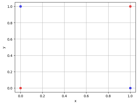
Not linearly separable in \(\mathbb{R}^2\)
3. Wiki /wiki/
Knowledge is a paradox. The more one understand, the more one realises the vastness of his ignorance.
4. CNN from scratch /wiki/ml/dl/cnn/
a convolutional neural network is a feedforward network with its linear layers put on a diet: instead of every unit seeing every input, each unit sees a small local window, and every window is processed by the same small set of weights. 𐃏 this page builds the operation from its definition, gets the geometry formulas straight, walks the canonical architectures, and ends with a convolution written in loops and checked against scipy (Goodfellow, Ian, 2016).
Comments