Predicting Life Expectancy
Intro
The focus here is on EDA (Exploratory Data Analysis) and investigating the best choice for the \(\lambda\) hyperparameter for LASSO and Ridge Regression.
We will be working on the Life Expectancy CSV data obtained from WHO.
Peeking at Data
We begin by viewing the columns of the Life Expectancy Dataframe:
import seaborn as sns
import pandas as pd
import matplotlib.pyplot as plt

pd.options.display.float_format = '{:.2f}'.format
le_df = pd.read_csv("life_expectancy.csv")
le_df.columns
We can then view the range of our life expectancy values with a box plot:
sns.boxplot(x=le_df['Life expectancy '])
plt.show()
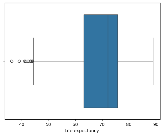
Life Expectancy Box Plot
From here we can glean
- the folks that died early at late 30’s, early 40’s;
- the minimum and maximum excluding these outliers (whiskers)
- the first and third Quartiles; and
- the mean (\(\mu\)) life expectancy
le_df.info()
Correlations
Then to produce a correlation matrix we would require exclusively continuous values. As such I have dropped those that are not:
le_df = le_df.drop(columns=['Country','Status'])
import numpy as np
corr_mat = le_df.corr()
mask = np.zeros_like(corr_mat, dtype=bool)
mask[np.triu_indices_from(mask)] = True

f, ax = plt.subplots(figsize=(20,19))
cmap=sns.diverging_palette(220,10, as_cmap=True)
sns.heatmap(corr_mat, mask=mask, cmap=cmap, vmax=.3, center=0,
              square=True, linewidths=.5, cbar_kws={"shrink": .5})
plt.show()
Note: We only need to view the lower / upper triangular section of the matrix due to the symmetry.
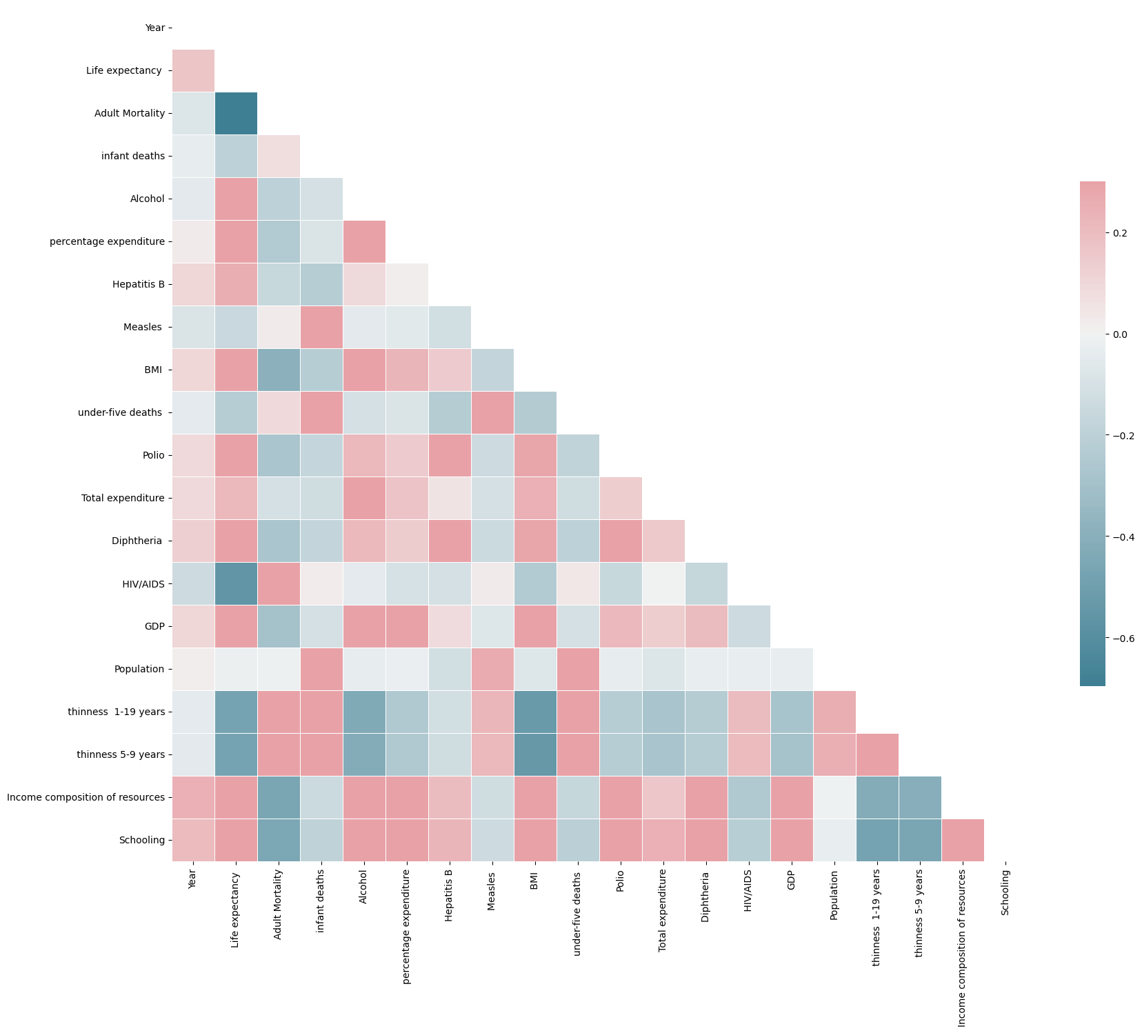
Correlation Heatmap
Letting our libraries continue doing the heavy lifting for us:
sns.pairplot(le_df)
plt.show()
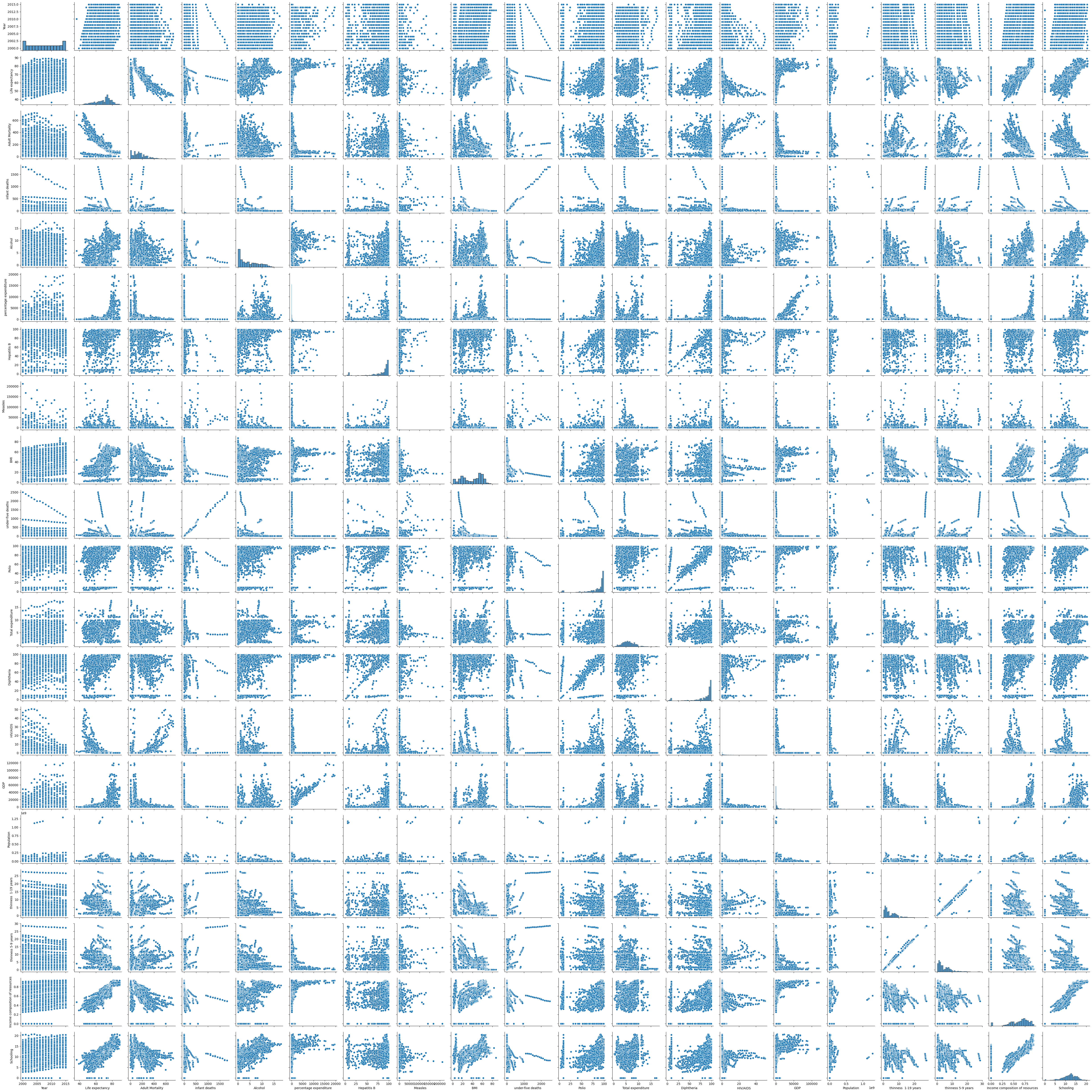
Correlation Pairplot
From here we learn that Adult Mortality is very negatively correlated with Life Expectancy (which makes sense). Also the 3 most positively correlated features with Life Expectancy are
- HIV/AIDS 0.753
- Income Comp of Resources 0.729
- Schooling 0.722
All of which are interesting in their own right.
Standard Scaling
Because we will be using regularised regression today and the penalties on weight will be affected by the magnitudes of the features we must first standardise our data:
from sklearn.preprocessing import StandardScaler

le_df_noNAN = le_df.dropna()
X = le_df_noNAN.drop(columns=["Life expectancy "])
y = le_df_noNAN["Life expectancy "].copy()

scaler = StandardScaler().fit(X)
scaled_X = scaler.transform(X)

print(f"Feature Means: {scaled_X.mean(axis=0)}")
print(f"Feature Variances: {scaled_X.var(axis=0)}")
Splitting Training and Test Data
Now we split the testing and training data
from sklearn.model_selection import train_test_split
X_train, X_test = train_test_split(X, test_size=0.2, random_state=73)
y_train, y_test = train_test_split(y, test_size=0.2, random_state=73)
Empiricism on Lambda (Ridge)
And start training a Ridge regression with varying values of the hyperparameter lambda:
%%time
import warnings
warnings.filterwarnings("ignore")
from sklearn.linear_model import Ridge
lambdas = [0.01, 0.1, 0.5, 1, 1.5, 2, 5, 10, 20, 30, 50, 100, 200, 300]
N = len(lambdas)
coefs_mat = np.zeros((X_train.shape[1], N))
for i in range(N):
  L = lambdas[i]
  ridge_lm = Ridge(alpha=L).fit(X_train, y_train)
  coefs_mat[:,i] = ridge_lm.coef_

plt.figure(figsize=(10,10))
for i in range(X_train.shape[1]):
  lab = "X" + str(i + 1)
  plt.plot(np.log(lambdas), coefs_mat[i], label=lab)
  plt.legend()
plt.xlabel(r"log($\lambda$)")
plt.ylabel("Estimated Coefficient")
plt.show()
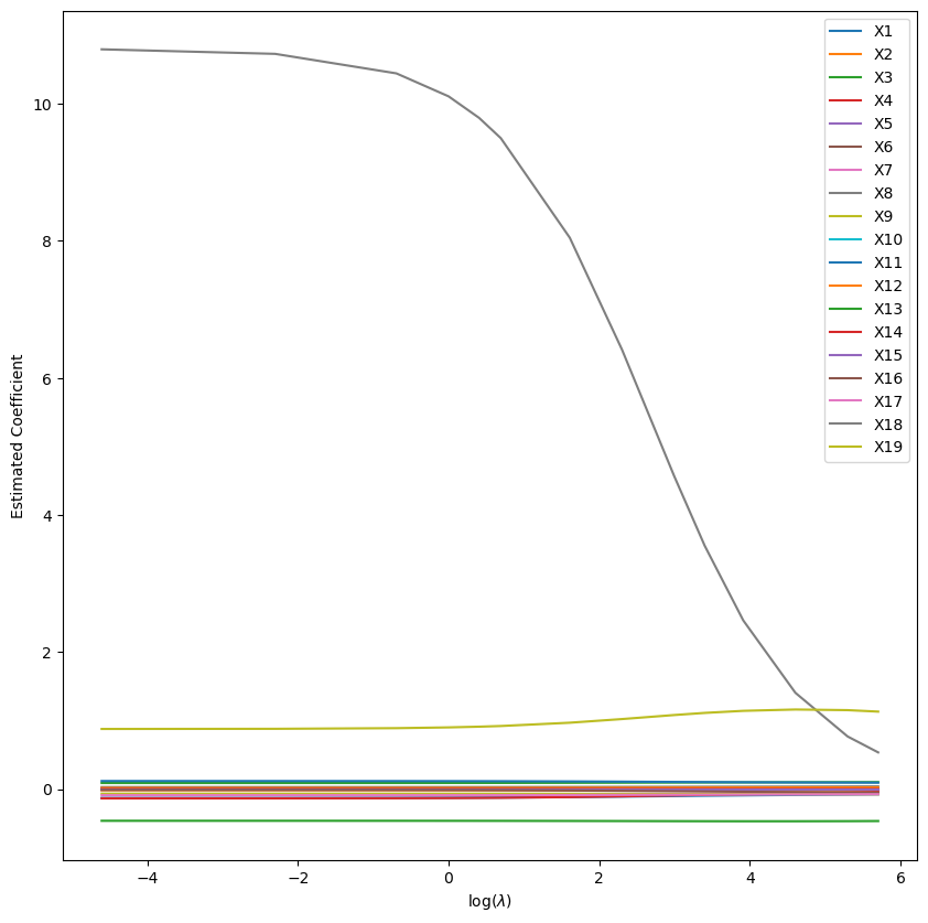
Ridge Regression Coefficients vs Lambda
We then find the best Lambda:
%%time
lambdas = np.arange(0,50.1,step=0.1)
n = X_train.shape[0]
N = lambdas.shape[0]
CV_score = np.zeros(N)
curIdx = 0
#X_train = X_train.to_numpy()
#y_train = y_train.to_numpy()
for L in lambdas:
  sq_errs = 0.
  for i in range(100):
    x_i = X_train[i]
    x_removed_i = np.delete(X_train, i, axis=0)
    y_i = y_train[i]
    y_removed_i = np.delete(y_train, i, axis=0)

    mod = Ridge(alpha=L).fit(x_removed_i, y_removed_i)
    sq_errs += (mod.predict(x_i.reshape(1,-1))-y_i)**2

  CV_score[curIdx] = sq_errs/n
  curIdx += 1

min_idx = np.argmin(CV_score)
plt.plot(lambdas, CV_score)
plt.xlabel(r"log($\lambda$)")
plt.ylabel("LOOCV (Ridge)")
plt.axvline(x=lambdas[min_idx], color='red')
plt.annotate(f"$\lambda = {lambdas[min_idx]}$", xy=(25,1800))
plt.show()
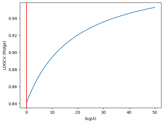
Ridge Regression Optimal Lambda
Empiricism on Lambda (LASSO)
We then repeat for our L1 regularisation model:
from sklearn.linear_model import Lasso
lambdas = [0.01, 0.1, 0.5, 1, 1.5, 2, 5, 10, 20, 30, 50, 100, 200, 300]
N = len(lambdas)
coefs_mat = np.zeros((X_train.shape[1], N))
for i in range(N):
  L = lambdas[i]
  ridge_lm = Lasso(alpha=L).fit(X_train, y_train)
  coefs_mat[:,i] = ridge_lm.coef_

plt.figure(figsize=(10,10))
for i in range(X_train.shape[1]):
  lab = "X" + str(i + 1)
  plt.plot(np.log(lambdas), coefs_mat[i], label=lab)
  plt.legend()
plt.xlabel(r"log($\lambda$)")
plt.ylabel("Estimated Coefficient")
plt.show()
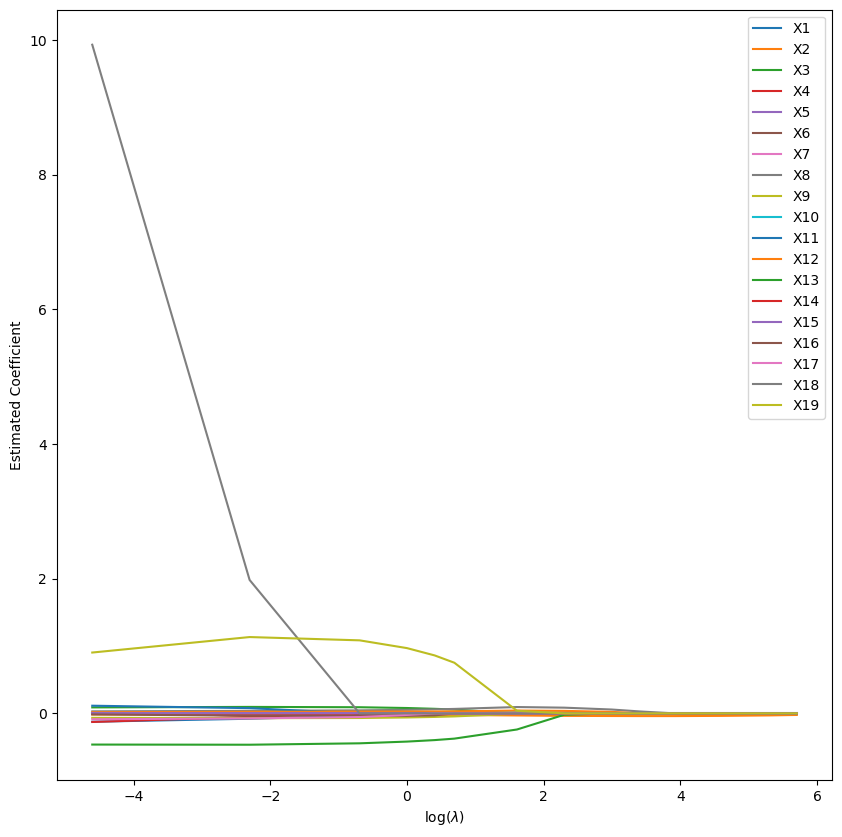
Lasso Regression Coefficients vs Lambda
Thus we find the optimal lambda to be…
%%time
lambdas = np.arange(0,50.1,step=0.1)
n = X_train.shape[0]
N = lambdas.shape[0]
CV_score = np.zeros(N)
curIdx = 0
#X_train = X_train.to_numpy()
#y_train = y_train.to_numpy()
for L in lambdas:
  sq_errs = 0.
  for i in range(20): #note we are not going to N
    x_i = X_train[i]
    x_removed_i = np.delete(X_train, i, axis=0)
    y_i = y_train[i]
    y_removed_i = np.delete(y_train, i, axis=0)

    mod = Lasso(alpha=L).fit(x_removed_i, y_removed_i)
    sq_errs += (mod.predict(x_i.reshape(1,-1))-y_i)**2

  CV_score[curIdx] = sq_errs/n
  curIdx += 1

min_idx = np.argmin(CV_score)
plt.plot(lambdas, CV_score)
plt.xlabel(r"log($\lambda$)")
plt.ylabel("LOOCV (Lasso)")
plt.axvline(x=lambdas[min_idx], color='red')
plt.annotate(f"$\lambda = {lambdas[min_idx]}$", xy=(25,1800))
plt.show()
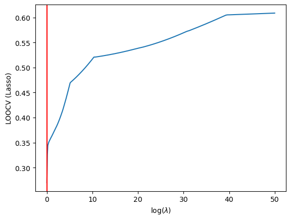
Lasso Regression Optimal Lambda
Results
It seems that in both situations we have fucked up. The LASSO and Ridge hyperparameters are being found to be 0. A quick fitting of the traning data to sklearn’s LassoCV model may help clear some confusion:
from sklearn.linear_model import LassoCV
from sklearn.metrics import mean_squared_error
m_lassoCV = LassoCV(cv=5).fit(X_train, y_train)
ypred_train_lassoCV = m_lassoCV.predict(X_train)
ypred_test_lassoCV = m_lassoCV.predict(X_test)
print(f"Mean Squared Error (TRAIN): {mean_squared_error(y_train,ypred_train_lassoCV)}")
print(f"Mean Squared Error (TEST) : {mean_squared_error(y_test, ypred_test_lassoCV)}")
print(f"With Lambda as {m_lassoCV.get_params()}")
Conclusion
The above shows that our analysis was not incorrect in attempting to determine the most optimal \(\lambda\)s, but rather a mistake has occurred in the preprocessing step causing the statistical signifance of my data to become muddled. In a later refactoring I may come back and improve my preprocessing, or abandon it completely in favour of a more homogenous dataset.
from sklearn.metrics import r2_score
print(f'Train Accuracy: {r2_score(ypred_train_lassoCV, y_train)}')
print(f'Test Accuracy: {r2_score(ypred_test_lassoCV, y_test)}')
Backlinks (11)
1. Ensemble Learning /wiki/ml/supervised/classification/ensembles/
one model is an opinion; a committee is an estimator. 𐃏 ensemble methods build many imperfect predictors and combine them, and the two great families attack opposite ends of the bias-variance decomposition: bagging averages low-bias, high-variance models to cancel their wobble; boosting stacks up high-bias, low-variance weak learners to build accuracy that none of them has alone.
2. Kernel Methods /wiki/ml/theory/kernel-methods/
kernel methods are the great arbitrage of classical machine learning: keep the algorithm linear — with all its convexity and closed forms — but run it in a feature space so large it can bend around anything, and never pay for that space explicitly. 𐃏 one identity powers everything: if your algorithm touches the data only through inner products, you may replace every \(\langle x, x’\rangle\) with a kernel \(k(x, x’)\) and thereby work in the implicit feature space of \(k\) — possibly infinite-dimensional — at the cost of an \(n \times n\) matrix.
3. Support Vector Machines (SVMs) /wiki/ml/supervised/classification/svm/
a linearly separable dataset admits infinitely many separating hyperplanes, and the perceptron will happily hand you whichever one it trips over first. 𐃏 the support vector machine asks a better question: of all the hyperplanes that separate the data, which one is farthest from everybody? the answer — the maximum-margin hyperplane — is determined by a handful of boundary points (the support vectors), drops out of a beautiful convex dual, and generalises via the kernel trick from lines to nearly anything.
4. The Bias-Variance Decomposition /wiki/ml/theory/bias-var/
there is exactly one theorem in machine learning that every practitioner rederives on a whiteboard at least once a year, and this is it. 𐃏 the squared-error risk of any learned predictor splits into three non-negative pieces — irreducible noise, squared bias, and variance — and every design decision you make (model class, regularisation strength, \(k\), ensemble size, early stopping) is secretly a transaction between the last two.
5. Curse of Dimensionality /wiki/ml/theory/curse-dim/
geometric intuition is trained in \(p \le 3\) and it does not survive the trip upstairs. 𐃏 in high dimensions the volume of a cube hides in its corners, every point is near the boundary, all pairwise distances look alike, and “local” neighbourhoods must stretch almost the full width of the space before they contain any data. every method that reasons from closeness — knn, kernel smoothers, rbf kernels — inherits these pathologies at once.
6. Locally Weighted Regression /wiki/ml/supervised/regression/locally-weighted/
a straight line is too rigid for a wiggly world, and a global degree-9 polynomial is a hostage negotiation. 𐃏 locally weighted regression (LWR — and its robust cousin LOWESS) takes the diplomatic route: fit the simplest possible model, but fit it freshly at every query point, paying attention only to the training points nearby.
motivation
- linear regression commits to one \(\theta\) for the whole input space. if the true \(f\) bends, the residue of that commitment is bias everywhere.
- the fix need not be a fancier global family. any smooth function is locally linear — taylor says so — so a linear fit weighted toward a neighbourhood of \(x_0\) can track an arbitrary smooth \(f\).
- the price: there is no longer a “trained model”. LWR is memory-based and non-parametric — like k-nearest neighbours, it keeps the entire training set and does all of its work at prediction time. training is \(O(1)\); every query costs a fresh weighted least-squares solve. 𐃏
the estimator
weighted least squares at a query point
fix a query \(x_0\). assign each training point a weight \(w_i(x_0) \ge 0\) that decays with distance from \(x_0\), then solve the weighted least-squares problem
7. No Free Lunch Theorem /wiki/ml/theory/no-free-lunch/
averaged over all possible problems, every learning algorithm is exactly as good as random guessing — and every optimiser is exactly as good as blind enumeration. 𐃏 this sounds like nihilism but is actually the sharpest possible argument for inductive bias: an algorithm can only beat chance on some problems by losing to chance on others, so the whole game of machine learning is choosing whose lunch to eat.
8. Performance Metrics for Machine Learning /wiki/ml/theory/perf-metrics/
a model is only as good as the number you judge it by, and most of the classic modelling disasters are really metric disasters — a fraud detector with \(99.9\%\) accuracy that never flags anything, a medical test tuned to a roc curve nobody deployed at the published threshold. 𐃏 this page is the field guide: what each metric measures, what it silently assumes, and which one to reach for when the classes are lopsided, the probabilities matter, or the target is continuous.
9. Regularised Regression /wiki/ml/supervised/regression/regularised/
this page collects the closed-form solutions to regularised regression (where they exist) and the iterative approximations we fall back on (where they don’t). 𐃏 along the way we will see that regularisation is not an ad-hoc hack but a perfectly sensible artefact of estimation: it drops straight out of MAP (maximum a posteriori) inference once you put a prior on the coefficients.
10. Wiki /wiki/
Knowledge is a paradox. The more one understand, the more one realises the vastness of his ignorance.
11. Machine Learning /wiki/ml/
Type 1 error
subtrees
- probabilistic graphical models — bayesian and markov networks, inference, hmms, learning
Comments