Solutions to Dobson & Barnett’s An Introduction to Generalized Linear Models
Solutions to every exercise in the fourth edition of Dobson & Barnett’s An Introduction to Generalized Linear Models (Chapman & Hall/CRC, 2018) — 78 exercises across 14 chapters, worked in R with the book’s own datasets from the dobson package, with executed code and committed output throughout. This is the MATH5806 text; the book is filed at An Introduction to Generalized Linear Models (Dobson & Barnett).
Introduction
Problem 1.1 — Let Y1 and Y2 be independent random variables with
Let \(Y_1\) and \(Y_2\) be independent random variables with \(Y_1 \sim N(1,3)\) and \(Y_2 \sim N(2,5)\). If \(W_1 = Y_1 + 2Y_2\) and \(W_2 = 4Y_1 - Y_2\), what is the joint distribution of \(W_1\) and \(W_2\)? (difficulty: \(\star\))
Write the transformation in matrix form. With \(\mathbf{y} = [Y_1, Y_2]^T\) and
\[ \mathbf{w} = \begin{pmatrix} W_1 \\ W_2 \end{pmatrix} = \mathbf{A}\mathbf{y}, \qquad \mathbf{A} = \begin{pmatrix} 1 & 2 \\ 4 & -1 \end{pmatrix}, \]
the two components of \(\mathbf{w}\) are linear combinations of independent Normal variables, so by Section 1.4.1 result 4 each of \(W_1, W_2\) is Normal; more than that, every linear combination \(a_1 W_1 + a_2 W_2\) is again a linear combination of \(Y_1\) and \(Y_2\) and hence Normal, which is exactly the condition for \(\mathbf{w}\) to be bivariate Normal. So only the mean vector and the variance-covariance matrix remain to be found.
Since the \(Y_i\) are independent,
\[ \boldsymbol{\mu}_y = \begin{pmatrix} 1 \\ 2 \end{pmatrix}, \qquad \mathbf{V}_y = \begin{pmatrix} 3 & 0 \\ 0 & 5 \end{pmatrix}. \]
By Equations (1.2) and (1.3), \(E(\mathbf{w}) = \mathbf{A}\boldsymbol{\mu}_y\) and \(\mathrm{var}(\mathbf{w}) = \mathbf{A}\mathbf{V}_y\mathbf{A}^T\). Componentwise,
\[ E(W_1) = 1 + 2(2) = 5, \qquad E(W_2) = 4(1) - 2 = 2, \] \[ \mathrm{var}(W_1) = 1^2(3) + 2^2(5) = 23, \qquad \mathrm{var}(W_2) = 4^2(3) + (-1)^2(5) = 53, \] \[ \mathrm{cov}(W_1, W_2) = \mathrm{cov}(Y_1 + 2Y_2,\; 4Y_1 - Y_2) = 4\,\mathrm{var}(Y_1) - 2\,\mathrm{var}(Y_2) = 4(3) - 2(5) = 2, \]
where the cross terms vanish because \(\mathrm{cov}(Y_1, Y_2) = 0\).
Hence
\[ \begin{pmatrix} W_1 \\ W_2 \end{pmatrix} \sim \mathrm{MVN}\left( \begin{pmatrix} 5 \\ 2 \end{pmatrix}, \begin{pmatrix} 23 & 2 \\ 2 & 53 \end{pmatrix} \right). \]
The matrix arithmetic, checked in R:
A  <- matrix(c(1, 2, 4, -1), nrow = 2, byrow = TRUE)
mu <- c(1, 2)
V  <- diag(c(3, 5))
A %*% mu
A %*% V %*% t(A)
     [,1]
[1,]    5
[2,]    2
     [,1] [,2]
[1,]   23    2
[2,]    2   53
Note that \(W_1\) and \(W_2\) are not independent even though \(Y_1\) and \(Y_2\) are: the correlation is \(2/\sqrt{23 \times 53} = 0.057\). It is small only by coincidence – the positive contribution \(4\,\mathrm{var}(Y_1) = 12\) nearly cancels the negative contribution \(-2\,\mathrm{var}(Y_2) = -10\). The covariance \(4\sigma_1^2 - 2\sigma_2^2\) vanishes exactly when \(\sigma_1^2 : \sigma_2^2 = 1 : 2\); here the ratio is \(3 : 5\), close to but not equal to \(1 : 2\). Had it been exactly \(1 : 2\), the two linear combinations would have been uncorrelated and, being jointly Normal, independent.
Problem 1.2 — Let Y1 and Y2 be independent random variables with Y1 \(\sim\) N(0, 1) and Y2 \(\sim\)
Let \(Y_1\) and \(Y_2\) be independent random variables with \(Y_1 \sim N(0,1)\) and \(Y_2 \sim N(3,4)\).
a. What is the distribution of \(Y_1^2\)? b. If \(\mathbf{y} = \begin{bmatrix} Y_1 \\ (Y_2 - 3)/2 \end{bmatrix}\), obtain an expression for \(\mathbf{y}^T\mathbf{y}\). What is its distribution? c. If \(\mathbf{y} = \begin{pmatrix} Y_1 \\ Y_2 \end{pmatrix}\) and its distribution is \(\mathbf{y} \sim \mathrm{MVN}(\boldsymbol{\mu}, \mathbf{V})\), obtain an expression for \(\mathbf{y}^T\mathbf{V}^{-1}\mathbf{y}\). What is its distribution? (difficulty: \(\star\))
Part (a): \(Y_1\) already has the standard Normal distribution, so by the definition of the central chi-squared distribution in Section 1.4.2 result 1 with \(n = 1\),
\[ Y_1^2 \sim \chi^2(1). \]
Part (b): The second element standardises \(Y_2\): since \(Y_2 \sim N(3, 4)\) has \(\mu_2 = 3\) and \(\sigma_2 = 2\), the variable \(Z_2 = (Y_2 - 3)/2 \sim N(0,1)\). Therefore
\[ \mathbf{y}^T\mathbf{y} = Y_1^2 + \frac{(Y_2 - 3)^2}{4}. \]
This is the sum of squares of two independent standard Normal variables, which is precisely the form in Equation (1.4) with \(n = 2\):
\[ \mathbf{y}^T\mathbf{y} \sim \chi^2(2). \]
Part (c): Here \(\mathbf{y}\) is not centred. Its mean vector and variance-covariance matrix are
\[ \boldsymbol{\mu} = \begin{pmatrix} 0 \\ 3 \end{pmatrix}, \qquad \mathbf{V} = \begin{pmatrix} 1 & 0 \\ 0 & 4 \end{pmatrix}, \qquad \mathbf{V}^{-1} = \begin{pmatrix} 1 & 0 \\ 0 & 1/4 \end{pmatrix}, \]
the off-diagonal entries being zero because \(Y_1\) and \(Y_2\) are independent. Hence
\[ \mathbf{y}^T\mathbf{V}^{-1}\mathbf{y} = Y_1^2 + \frac{Y_2^2}{4}. \]
By Section 1.4.2 result 6, \(\mathbf{y}^T\mathbf{V}^{-1}\mathbf{y}\) has the non-central chi-squared distribution \(\chi^2(n, \lambda)\) with \(n = 2\) degrees of freedom and non-centrality parameter
\[ \lambda = \boldsymbol{\mu}^T\mathbf{V}^{-1}\boldsymbol{\mu} = 0^2 + \frac{3^2}{4} = \frac{9}{4} = 2.25, \]
so \(\mathbf{y}^T\mathbf{V}^{-1}\mathbf{y} \sim \chi^2(2, 2.25)\).
The contrast between (b) and (c) is the whole point of the exercise. Subtracting the mean before standardising gives a central chi-squared; failing to subtract it leaves the squared standardised mean behind as the non-centrality parameter. Note \(\lambda = 2.25 = (\mu_2/\sigma_2)^2\), and indeed \(\mathbf{y}^T\mathbf{y}\) from (b) equals \(\mathbf{y}^T\mathbf{V}^{-1}\mathbf{y}\) from (c) with \(Y_2\) replaced by \(Y_2 - 3\).
A simulation confirms the moments of (c), using \(E = n + \lambda\) and \(\mathrm{var} = 2n + 4\lambda\) from Section 1.4.2 result 4:
set.seed(1)
n  <- 2e6
Y1 <- rnorm(n, 0, 1)
Y2 <- rnorm(n, 3, 2)
Q  <- Y1^2 + Y2^2 / 4
c(mean = mean(Q), var = var(Q))
c(theory.mean = 2 + 2.25, theory.var = 2 * 2 + 4 * 2.25)
ks.test(sample(Q, 5000), "pchisq", df = 2, ncp = 2.25)$p.value
     mean       var
 4.251925 13.007515
theory.mean  theory.var
       4.25       13.00
[1] 0.4517404
The simulated mean and variance match the theoretical \(4.25\) and \(13\), and a Kolmogorov-Smirnov test against \(\chi^2(2, 2.25)\) gives \(p = 0.45\), so there is no evidence against the claimed distribution.
Problem 1.3 — Let the joint distribution of Y1 and Y2 be MVN(µ , V) with
Let the joint distribution of \(Y_1\) and \(Y_2\) be \(\mathrm{MVN}(\boldsymbol{\mu}, \mathbf{V})\) with
\[ \boldsymbol{\mu} = \begin{pmatrix} 2 \\ 3 \end{pmatrix} \quad \text{and} \quad \mathbf{V} = \begin{pmatrix} 4 & 1 \\ 1 & 9 \end{pmatrix}. \]
a. Obtain an expression for \((\mathbf{y} - \boldsymbol{\mu})^T\mathbf{V}^{-1}(\mathbf{y} - \boldsymbol{\mu})\). What is its distribution? b. Obtain an expression for \(\mathbf{y}^T\mathbf{V}^{-1}\mathbf{y}\). What is its distribution? (difficulty: \(\star\star\))
Both parts need \(\mathbf{V}^{-1}\). For a \(2 \times 2\) matrix, \(\det \mathbf{V} = 4(9) - 1(1) = 35\) and
\[ \mathbf{V}^{-1} = \frac{1}{35}\begin{pmatrix} 9 & -1 \\ -1 & 4 \end{pmatrix}. \]
Note \(\det \mathbf{V} > 0\) and \(v_{11} = 4 > 0\), so \(\mathbf{V}\) is positive definite by the determinant criterion of Section 1.5 result 3, and the inverse exists as required.
Part (a): Writing \(u_1 = y_1 - 2\) and \(u_2 = y_2 - 3\), the quadratic form expands as
\[ (\mathbf{y} - \boldsymbol{\mu})^T\mathbf{V}^{-1}(\mathbf{y} - \boldsymbol{\mu}) = \frac{1}{35}\left[ 9u_1^2 - 2u_1u_2 + 4u_2^2 \right], \]
that is,
\[ \frac{1}{35}\left[ 9(y_1 - 2)^2 - 2(y_1 - 2)(y_2 - 3) + 4(y_2 - 3)^2 \right]. \]
The cross term picks up a factor of \(2\) because the two off-diagonal entries \(-1/35\) are equal. Since \(\mathbf{V}\) is non-singular, Equation (1.5) applies directly with \(n = 2\):
\[ (\mathbf{y} - \boldsymbol{\mu})^T\mathbf{V}^{-1}(\mathbf{y} - \boldsymbol{\mu}) \sim \chi^2(2). \]
Part (b): The same algebra without centring gives
\[ \mathbf{y}^T\mathbf{V}^{-1}\mathbf{y} = \frac{1}{35}\left[ 9y_1^2 - 2y_1y_2 + 4y_2^2 \right]. \]
By Section 1.4.2 result 6 this has the non-central chi-squared distribution with \(2\) degrees of freedom and non-centrality parameter
\[ \lambda = \boldsymbol{\mu}^T\mathbf{V}^{-1}\boldsymbol{\mu} = \frac{1}{35}\left[ 9(2)^2 - 2(2)(3) + 4(3)^2 \right] = \frac{36 - 12 + 36}{35} = \frac{60}{35} = \frac{12}{7} \approx 1.714, \]
so \(\mathbf{y}^T\mathbf{V}^{-1}\mathbf{y} \sim \chi^2(2, 12/7)\).
Confirming the inverse and \(\lambda\) in R:
mu <- c(2, 3)
V  <- matrix(c(4, 1, 1, 9), nrow = 2)
det(V)
Vinv <- solve(V)
35 * Vinv
lambda <- drop(t(mu) %*% Vinv %*% mu)
c(lambda = lambda, as.fraction = 60 / 35)
[1] 35
     [,1] [,2]
[1,]    9   -1
[2,]   -1    4
     lambda as.fraction
   1.714286    1.714286
Interpretation: the degrees of freedom are the same in both parts because \(\mathbf{V}^{-1}\) has full rank \(2\) (Section 1.5 result 4). What differs is the location. In (a) the quadratic form is a squared Mahalanobis distance from the mean, and it has expected value \(2\); in (b) it is measured from the origin, and the extra distance of \(\boldsymbol{\mu}\) from \(\mathbf{0}\) inflates the expectation to \(n + \lambda = 2 + 12/7 \approx 3.71\). Quantities of exactly form (a) reappear in later chapters as goodness-of-fit statistics; form (b) is what arises under an alternative hypothesis, and \(\lambda\) is what drives the power of the test.
Problem 1.4 — Let Y1 , . . . ,Yn be independent random variables each with the distribution
Let \(Y_1, \ldots, Y_n\) be independent random variables each with the distribution \(N(\mu, \sigma^2)\). Let
\[ \overline{Y} = \frac{1}{n}\sum_{i=1}^{n} Y_i \quad \text{and} \quad S^2 = \frac{1}{n-1}\sum_{i=1}^{n}(Y_i - \overline{Y})^2. \]
a. What is the distribution of \(\overline{Y}\)? b. Show that \(S^2 = \frac{1}{n-1}\left[ \sum_{i=1}^{n}(Y_i - \mu)^2 - n(\overline{Y} - \mu)^2 \right]\). c. From (b) it follows that \(\sum (Y_i - \mu)^2/\sigma^2 = (n-1)S^2/\sigma^2 + \left[ (\overline{Y} - \mu)^2 n/\sigma^2 \right]\). How does this allow you to deduce that \(\overline{Y}\) and \(S^2\) are independent? d. What is the distribution of \((n-1)S^2/\sigma^2\)? e. What is the distribution of \(\dfrac{\overline{Y} - \mu}{S/\sqrt{n}}\)? (difficulty: \(\star\star\))
Part (a): \(\overline{Y} = \sum a_i Y_i\) with every \(a_i = 1/n\), so by Section 1.4.1 result 4,
\[ \overline{Y} \sim N\!\left( \sum \frac{1}{n}\mu, \; \sum \frac{1}{n^2}\sigma^2 \right) = N\!\left( \mu, \frac{\sigma^2}{n} \right). \]
Part (b): Insert and remove \(\mu\) inside the square, writing \(Y_i - \overline{Y} = (Y_i - \mu) - (\overline{Y} - \mu)\). Then
\[ \sum_{i=1}^{n}(Y_i - \overline{Y})^2 = \sum (Y_i - \mu)^2 - 2(\overline{Y} - \mu)\sum (Y_i - \mu) + n(\overline{Y} - \mu)^2. \]
The middle sum is \(\sum (Y_i - \mu) = n\overline{Y} - n\mu = n(\overline{Y} - \mu)\), so the cross term equals \(-2n(\overline{Y} - \mu)^2\) and
\[ \sum_{i=1}^{n}(Y_i - \overline{Y})^2 = \sum (Y_i - \mu)^2 - n(\overline{Y} - \mu)^2. \]
Dividing by \(n-1\) gives the required identity. This is an algebraic identity: it holds for any numbers, no distributional assumption is used.
Part (c): Divide the identity by \(\sigma^2\) to get the decomposition stated in the question,
\[ \underbrace{\sum \frac{(Y_i - \mu)^2}{\sigma^2}}_{Q} = \underbrace{\frac{(n-1)S^2}{\sigma^2}}_{Q_1} + \underbrace{\frac{n(\overline{Y} - \mu)^2}{\sigma^2}}_{Q_2}. \]
Each \(Y_i - \mu \sim N(0, \sigma^2)\) independently, so \(Q \sim \chi^2(n)\) by Equation (1.4), and \(Q_1, Q_2\) are quadratic forms in the \(Y_i - \mu\). Their degrees of freedom (ranks) are \(m_1 = n-1\) and \(m_2 = 1\): \(Q_2\) is a single squared linear combination, hence rank \(1\), and \(Q_1\) is the sum of squared deviations about their own mean, whose matrix \(\mathbf{I} - \frac{1}{n}\mathbf{J}\) is idempotent with trace \(n-1\). Since \(m_1 + m_2 = n\), Cochran’s theorem (Section 1.5 result 5) applies and gives that \(Q_1\) and \(Q_2\) are independent, with \(Q_1 \sim \chi^2(n-1)\) and \(Q_2 \sim \chi^2(1)\).
Strictly, Cochran’s theorem delivers independence of \(S^2\) and \((\overline{Y} - \mu)^2\), not of \(S^2\) and \(\overline{Y}\) itself. The gap is easily closed and worth stating explicitly rather than glossing over: \(\mathrm{cov}(\overline{Y},\, Y_i - \overline{Y}) = \sigma^2/n - \sigma^2/n = 0\) for every \(i\), and the vector \((\overline{Y}, Y_1 - \overline{Y}, \ldots, Y_n - \overline{Y})\) is multivariate Normal because all its entries are linear in the \(Y_i\). Zero covariance plus joint Normality gives independence of \(\overline{Y}\) from the whole residual vector, hence from \(S^2\), which is a function of that vector alone. With that supplement the deduction is rigorous.
Part (d): From (c),
\[ \frac{(n-1)S^2}{\sigma^2} \sim \chi^2(n-1). \]
The single degree of freedom lost is exactly the one spent estimating \(\mu\) by \(\overline{Y}\), which is what the decomposition in (c) makes visible. It also gives \(E(S^2) = \sigma^2\) immediately, since \(E[\chi^2(n-1)] = n-1\).
Part (e): Standardise the numerator using (a): \(Z = (\overline{Y} - \mu)/(\sigma/\sqrt{n}) \sim N(0,1)\). Let \(X^2 = (n-1)S^2/\sigma^2 \sim \chi^2(n-1)\), independent of \(Z\) by (c). Then
\[ \frac{\overline{Y} - \mu}{S/\sqrt{n}} = \frac{(\overline{Y} - \mu)/(\sigma/\sqrt{n})}{S/\sigma} = \frac{Z}{\left[ X^2/(n-1) \right]^{1/2}}, \]
since \(S/\sigma = [X^2/(n-1)]^{1/2}\). That is exactly the definition of the t-distribution in Equation (1.6), so
\[ \frac{\overline{Y} - \mu}{S/\sqrt{n}} \sim t(n-1). \]
The unknown \(\sigma\) has cancelled, which is why this statistic is usable in practice: it is the one-sample t-statistic.
A simulation with \(n = 8\), \(\mu = 10\), \(\sigma = 3\) checks (c), (d) and (e) numerically:
set.seed(42)
n <- 8; mu <- 10; sigma <- 3; B <- 2e5
sim  <- matrix(rnorm(n * B, mu, sigma), nrow = B)
ybar <- rowMeans(sim)
s2   <- apply(sim, 1, var)
c(cor.ybar.s2 = cor(ybar, s2))
Q1 <- (n - 1) * s2 / sigma^2
c(mean.Q1 = mean(Q1), df = n - 1, var.Q1 = var(Q1), two.df = 2 * (n - 1))
Tstat <- (ybar - mu) / sqrt(s2 / n)
c(mean.T = mean(Tstat), var.T = var(Tstat), t.var = (n - 1) / (n - 3))
ks.test(sample(Tstat, 5000), "pt", df = n - 1)$p.value
  cor.ybar.s2
-0.0006370237
  mean.Q1        df    var.Q1    two.df
 7.007965  7.000000 14.053002 14.000000
      mean.T        var.T        t.var
0.0002216423 1.4003904492 1.4000000000
[1] 0.4874567
The sample correlation between \(\overline{Y}\) and \(S^2\) is essentially zero, consistent with (c). \(Q_1\) has simulated mean \(7.01\) and variance \(14.05\) against the \(\chi^2(7)\) values \(7\) and \(14\), confirming (d). The t-statistic has simulated variance \(1.400\) against the \(t(7)\) value \((n-1)/(n-3) = 1.4\), and a Kolmogorov-Smirnov test against \(t(7)\) gives \(p = 0.49\), confirming (e). Note the variance exceeds \(1\): the heavier tails of \(t(7)\) relative to \(N(0,1)\) are the price of estimating \(\sigma\).
Problem 1.5 — This exercise is a continuation of the example in Section 1.6.2 in which
This exercise is a continuation of the example in Section 1.6.2 in which \(Y_1, \ldots, Y_n\) are independent Poisson random variables with the parameter \(\theta\).
a. Show that \(E(Y_i) = \theta\) for \(i = 1, \ldots, n\). b. Suppose \(\theta = e^{\beta}\). Find the maximum likelihood estimator of \(\beta\). c. Minimize \(S = \sum \left( Y_i - e^{\beta} \right)^2\) to obtain a least squares estimator of \(\beta\). (difficulty: \(\star\star\))
Part (a): With \(f(y_i; \theta) = \theta^{y_i}e^{-\theta}/y_i!\) for \(y_i = 0, 1, 2, \ldots\),
\[ E(Y_i) = \sum_{y=0}^{\infty} y\,\frac{\theta^{y}e^{-\theta}}{y!} = \sum_{y=1}^{\infty} \frac{\theta^{y}e^{-\theta}}{(y-1)!}, \]
the \(y = 0\) term contributing nothing. Substituting \(z = y - 1\) and taking one factor of \(\theta\) outside,
\[ E(Y_i) = \theta e^{-\theta}\sum_{z=0}^{\infty}\frac{\theta^{z}}{z!} = \theta e^{-\theta}e^{\theta} = \theta, \]
using the exponential series \(\sum_{z \ge 0} \theta^{z}/z! = e^{\theta}\).
Part (b): Reparameterising the log-likelihood of Section 1.6.2 by \(\theta = e^{\beta}\),
\[ l(\beta; \mathbf{y}) = \left( \sum y_i \right)\beta - n e^{\beta} - \sum \log y_i!, \]
since \(\log \theta = \beta\) and \(n\theta = ne^{\beta}\). Differentiating,
\[ \frac{dl}{d\beta} = \sum y_i - n e^{\beta}. \]
Setting this to zero gives \(e^{\beta} = \overline{y}\), so
\[ \widehat{\beta} = \log \overline{y}, \]
provided \(\overline{y} > 0\). The second derivative is \(d^2l/d\beta^2 = -ne^{\beta} < 0\) everywhere, so \(l\) is strictly concave in \(\beta\) and \(\widehat{\beta}\) is the unique maximum, as required by the check in Section 1.6.1.
This is the invariance property of maximum likelihood estimators in action: \(\beta = g(\theta) = \log\theta\) is a one-to-one function of \(\theta\), so \(\widehat{\beta} = g(\widehat{\theta}\,) = \log \overline{y}\) without redoing the calculus. Note also that \(\beta\) is the natural parameter of the Poisson distribution, and \(\theta = e^{\beta}\) is the log link that will define the Poisson generalized linear model in Chapter 9.
Part (c): Put \(u = e^{\beta}\), so \(S = \sum (Y_i - u)^2\) and, by the chain rule,
\[ \frac{dS}{d\beta} = \frac{dS}{du}\cdot\frac{du}{d\beta} = \left[ -2\sum (Y_i - u) \right] e^{\beta} = -2e^{\beta}\left( \sum Y_i - n e^{\beta} \right). \]
Because \(e^{\beta} > 0\) for every real \(\beta\), the derivative vanishes only where \(\sum Y_i = ne^{\beta}\), that is at
\[ \widetilde{\beta} = \log \overline{y}. \]
To confirm a minimum, note \(d^2S/d\beta^2 = e^{2\beta}\,d^2S/du^2 + (dS/du)e^{\beta}\), and at the stationary point \(dS/du = 0\), leaving \(e^{2\beta}(2n) > 0\).
So the least squares and maximum likelihood estimators coincide here, illustrating comment 2 of Section 1.6.4. The agreement is not automatic: least squares needs only \(E(Y_i) = e^{\beta}\) whereas maximum likelihood needs the full Poisson specification. They agree because both estimating equations reduce to the same moment condition \(\sum(Y_i - e^{\beta}) = 0\). The agreement also relies on the \(Y_i\) being identically distributed here: all \(n\) variables share the single parameter \(\theta\), so \(\mathrm{var}(Y_i) = \theta\) is the same for every \(i\) and unweighted least squares is already the correctly weighted one (Section 1.6.3, weights \(w_i = 1/\sigma_i^2\)). Once explanatory variables enter and the means differ across observations, the Poisson variances differ too, since variance equals mean, the two methods separate, and it is weighted least squares that tracks maximum likelihood.
Applying this to the tropical cyclone data of Table 1.2, where Section 1.6.5 reports \(\widehat{\theta} = 72/13 = 5.538\):
library(dobson)
data(cyclones)
y <- cyclones$number
c(n = length(y), total = sum(y), ybar = mean(y))
betahat <- log(mean(y))
c(betahat = betahat, exp.betahat = exp(betahat))

negll <- function(b) -sum(y * b - exp(b) - lfactorial(y))
opt <- optimize(negll, interval = c(-5, 5), tol = 1e-10)
c(numerical.betahat = opt$minimum, closed.form = betahat)

ss  <- function(b) sum((y - exp(b))^2)
opt2 <- optimize(ss, interval = c(-5, 5), tol = 1e-10)
c(least.squares.betahat = opt2$minimum)

coef(glm(y ~ 1, family = poisson(link = "log")))
        n     total      ybar
13.000000 72.000000  5.538462
    betahat exp.betahat
   1.711717    5.538462
numerical.betahat       closed.form
         1.711717          1.711717
least.squares.betahat
             1.711717
(Intercept)
   1.711717
All four routes agree on \(\widehat{\beta} = 1.7117\), and \(e^{\widehat{\beta}} = 5.538\) recovers \(\widehat{\theta}\), confirming (b) and (c). The intercept-only Poisson generalized linear model with log link, which is what the last line fits, returns the identical estimate – this exercise is the simplest possible instance of the machinery developed in the rest of the book.
Problem 1.6 — The data in Table 1.4 are the numbers of females and males in the progeny
The data in Table 1.4 are the numbers of females and males in the progeny of 16 female light brown apple moths in Muswellbrook, New South Wales, Australia (from Lewis, 1987). Table 1.4 lists, for progeny groups \(1\) to \(16\) respectively, the numbers of females \(18, 31, 34, 33, 27, 33, 28, 23, 33, 12, 19, 25, 14, 4, 22, 7\) and the corresponding numbers of males \(11, 22, 27, 29, 24, 29, 25, 26, 38, 14, 23, 31, 20, 6, 34, 12\).
a. Calculate the proportion of females in each of the 16 groups of progeny. b. Let \(Y_i\) denote the number of females and \(n_i\) the number of progeny in each group (\(i = 1, \ldots, 16\)). Suppose the \(Y_i\)’s are independent random variables each with the Binomial distribution
\[ f(y_i; \theta) = \binom{n_i}{y_i}\theta^{y_i}(1 - \theta)^{n_i - y_i}. \]
Find the maximum likelihood estimator of \(\theta\) using calculus and evaluate it for these data. c. Use a numerical method to estimate \(\widehat{\theta}\) and compare the answer with the one from (b). (difficulty: \(\star\star\))
Part (a): The group size is \(n_i = (\text{females})_i + (\text{males})_i\) and the proportion female is \(p_i = y_i/n_i\).
library(dobson)
data(moths)
moths$n <- moths$females + moths$males
moths$p <- moths$females / moths$n
print(round(moths[, c("group", "females", "n", "p")], 3), row.names = FALSE)
c(total.females = sum(moths$females), total.progeny = sum(moths$n),
  theta.hat = sum(moths$females) / sum(moths$n))
 group females  n     p
     1      18 29 0.621
     2      31 53 0.585
     3      34 61 0.557
     4      33 62 0.532
     5      27 51 0.529
     6      33 62 0.532
     7      28 53 0.528
     8      23 49 0.469
     9      33 71 0.465
    10      12 26 0.462
    11      19 42 0.452
    12      25 56 0.446
    13      14 34 0.412
    14       4 10 0.400
    15      22 56 0.393
    16       7 19 0.368
total.females total.progeny     theta.hat
  363.0000000   734.0000000     0.4945504
The proportions range from \(0.368\) to \(0.621\), scattered around one half. The smallest groups carry the least information: group \(14\) has only \(10\) progeny, so its proportion of \(0.400\) is one female away from \(0.500\).
Part (b): The likelihood function for the whole sample is the product over the \(16\) independent groups,
\[ L(\theta; \mathbf{y}) = \prod_{i=1}^{16}\binom{n_i}{y_i}\theta^{y_i}(1 - \theta)^{n_i - y_i}, \]
so the log-likelihood is
\[ l(\theta; \mathbf{y}) = \sum_{i=1}^{16}\log\binom{n_i}{y_i} + \left( \sum y_i \right)\log\theta + \left( \sum n_i - \sum y_i \right)\log(1 - \theta). \]
The binomial coefficients do not involve \(\theta\) and so play no part in the optimisation, exactly as the \(\sum \log y_i!\) term did not in Section 1.6.5. Write \(N = \sum n_i\) and \(T = \sum y_i\). Then, following Equation (1.9),
\[ \frac{dl}{d\theta} = \frac{T}{\theta} - \frac{N - T}{1 - \theta} = \frac{T(1 - \theta) - (N - T)\theta}{\theta(1 - \theta)} = \frac{T - N\theta}{\theta(1 - \theta)}. \]
Setting the numerator to zero gives
\[ \widehat{\theta} = \frac{T}{N} = \frac{\sum_{i=1}^{16} y_i}{\sum_{i=1}^{16} n_i}. \]
For the maximum check,
\[ \frac{d^2l}{d\theta^2} = -\frac{T}{\theta^2} - \frac{N - T}{(1 - \theta)^2} < 0 \]
for all \(\theta \in (0,1)\) whenever \(0 < T < N\), so \(l\) is strictly concave and \(\widehat{\theta}\) is the unique interior maximum. From the output above, \(T = 363\) and \(N = 734\), so
\[ \widehat{\theta} = \frac{363}{734} = 0.4946. \]
Note that this is the pooled proportion, not the average of the \(16\) group proportions. The estimator weights each group by its size \(n_i\), which is correct because larger groups carry more information about \(\theta\).
Part (c): Three numerical routes, none of which uses the closed form: direct maximisation of \(l^*(\theta) = \sum [ y_i \log\theta + (n_i - y_i)\log(1 - \theta) ]\) with optimize, a bisection search in the spirit of Table 1.3, and the intercept-only binomial generalized linear model.
y <- moths$females; n <- moths$n

lstar <- function(th) sum(y * log(th) + (n - y) * log(1 - th))
opt <- optimize(lstar, interval = c(0.001, 0.999), maximum = TRUE, tol = 1e-12)
c(optimize = opt$maximum, closed.form = sum(y) / sum(n))

lo <- 0.30; hi <- 0.70
for (k in 1:20) {
  mid <- (lo + hi) / 2
  if (lstar(mid + 1e-8) > lstar(mid - 1e-8)) lo <- mid else hi <- mid
}
c(bisection = (lo + hi) / 2)

fit <- glm(cbind(females, males) ~ 1, family = binomial, data = moths)
c(glm.theta = plogis(coef(fit)))
   optimize closed.form
  0.4945504   0.4945504
bisection
0.4945505
glm.theta.(Intercept)
            0.4945504
All three numerical answers agree with the calculus answer of (b) to at least six decimal places; the bisection differs only in the seventh, because \(20\) halvings of an interval of width \(0.4\) leave a resolution of about \(4 \times 10^{-7}\). This is the same bisection idea used for the cyclone data in Section 1.6.5, and it makes the same point: when the closed form is unavailable – which is the normal situation for the generalized linear models of later chapters – a numerical search recovers the estimate without any loss of accuracy that matters.
Finally, inference and adequacy. The estimate is only useful with a standard error and a check that the single-\(\theta\) model is tenable.
th <- sum(y) / sum(n)
se <- sqrt(th * (1 - th) / sum(n))
c(theta.hat = th, se = se, lower = th - 1.96 * se, upper = th + 1.96 * se)
c(z.vs.half = (th - 0.5) / se, p.value = 2 * pnorm(-abs((th - 0.5) / se)))
c(resid.dev = deviance(fit), df = df.residual(fit),
  p.het = pchisq(deviance(fit), df.residual(fit), lower.tail = FALSE))
 theta.hat         se      lower      upper
0.49455041 0.01845424 0.45838010 0.53072072
 z.vs.half    p.value
-0.2953029  0.7677625
 resid.dev         df      p.het
11.9288136 15.0000000  0.6844091
The estimated sex ratio is \(\widehat{\theta} = 0.495\) with standard error \(0.018\) and approximate \(95\%\) confidence interval \((0.458, 0.531)\). This comfortably contains \(0.5\): the test of \(H_0: \theta = 0.5\) gives \(z = -0.30\), \(p = 0.77\), so there is no evidence that light brown apple moth progeny depart from an even sex ratio, which is what Mendelian sex determination predicts.
The residual deviance of \(11.93\) on \(15\) degrees of freedom (the \(16\) groups less the one fitted parameter) tests whether a common \(\theta\) suffices, against the alternative that each mother has her own sex ratio. With \(p = 0.68\) there is no evidence of heterogeneity between mothers – the spread of the \(16\) proportions in (a) is no more than binomial sampling variation would produce. The figure below makes this visual: the observed proportions fan out for small \(n_i\) and tighten for large \(n_i\) in the manner the binomial variance \(\theta(1-\theta)/n_i\) requires, and all \(16\) sit inside the pointwise \(95\%\) band.
p  <- y / n
th <- sum(y) / sum(n)
par(mfrow = c(1, 2))
plot(n, p, pch = 19, ylim = c(0.3, 0.7), xlab = "progeny in group (n_i)",
     ylab = "proportion female", main = "Proportions vs group size")
abline(h = th, lty = 2); abline(h = 0.5, lty = 3, col = "grey40")
curve(th + 1.96 * sqrt(th * (1 - th) / x), add = TRUE, col = "grey50")
curve(th - 1.96 * sqrt(th * (1 - th) / x), add = TRUE, col = "grey50")
legend("topright", c("MLE 0.4946", "0.5", "95% binomial band"),
       lty = c(2, 3, 1), col = c("black", "grey40", "grey50"), bty = "n")
tt <- seq(0.30, 0.70, length.out = 400)
ls <- sapply(tt, function(t) sum(y * log(t) + (n - y) * log(1 - t)))
plot(tt, ls, type = "l", xlab = expression(theta), ylab = "log-likelihood (l*)",
     main = "Log-likelihood function")
abline(v = th, lty = 2)
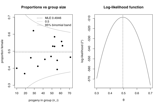
The right-hand panel is the analogue of Figure 1.2 for these data: a single smooth peak at \(\widehat{\theta} = 0.4946\), sharply curved, which is why the standard error is small. The curvature at the maximum is \(-d^2l/d\theta^2 = N/[\theta(1-\theta)] = 2936.3\), and \(1/\sqrt{2936.3} = 0.01845\) reproduces the standard error above – the connection between likelihood curvature and precision that Chapter 5 develops formally.
Model Fitting
Problem 2.1 — Genetically similar seeds are randomly assigned to be raised in either a
Genetically similar seeds are randomly assigned to be raised in either a nutritionally enriched environment (treatment group) or standard conditions (control group) using a completely randomized experimental design. After a predetermined time all plants are harvested, dried and weighed. The results, expressed in grams, for 20 plants in each group are shown in Table 2.7.
Table 2.7 (Dried weight of plants grown under two conditions) has two columns. The treatment group values, read down the two printed sub-columns, are \(4.81, 4.17, 4.41, 3.59, 5.87, 3.83, 6.03, 4.98, 4.90, 5.75\) and \(5.36, 3.48, 4.69, 4.44, 4.89, 4.71, 5.48, 4.32, 5.15, 6.34\). The control group values are \(4.17, 3.05, 5.18, 4.01, 6.11, 4.10, 5.17, 3.57, 5.33, 5.59\) and \(4.66, 5.58, 3.66, 4.50, 3.90, 4.61, 5.62, 4.53, 6.05, 5.14\).
We want to test whether there is any difference in yield between the two groups. Let \(Y_{jk}\) denote the \(k\)th observation in the \(j\)th group where \(j = 1\) for the treatment group, \(j = 2\) for the control group and \(k = 1, \ldots, 20\) for both groups. Assume that the \(Y_{jk}\)’s are independent random variables with \(Y_{jk} \sim \mathrm{N}(\mu_j, \sigma^2)\). The null hypothesis \(\mathrm{H}_0 : \mu_1 = \mu_2 = \mu\), that there is no difference, is to be compared with the alternative hypothesis \(\mathrm{H}_1 : \mu_1 \neq \mu_2\).
- a.
- Conduct an exploratory analysis of the data looking at the distributions for each group (e.g., using dot plots, stem and leaf plots or Normal probability plots) and calculate summary statistics (e.g., means, medians, standard derivations, maxima and minima). What can you infer from these investigations?
- b.
- Perform an unpaired \(t\)-test on these data and calculate a 95% confidence interval for the difference between the group means. Interpret these results.
- c.
- The following models can be used to test the null hypothesis \(\mathrm{H}_0\) against the alternative hypothesis \(\mathrm{H}_1\), where \[ \mathrm{H}_0 : \mathrm{E}(Y_{jk}) = \mu; \quad Y_{jk} \sim \mathrm{N}(\mu, \sigma^2), \] \[ \mathrm{H}_1 : \mathrm{E}(Y_{jk}) = \mu_j; \quad Y_{jk} \sim \mathrm{N}(\mu_j, \sigma^2), \] for \(j = 1, 2\) and \(k = 1, \ldots, 20\). Find the maximum likelihood and least squares estimates of the parameters \(\mu, \mu_1\) and \(\mu_2\), assuming \(\sigma^2\) is a known constant.
- d.
- Show that the minimum values of the least squares criteria are \[ \text{for } \mathrm{H}_0, \quad \widehat{S}_0 = \sum\sum (Y_{jk} - \overline{Y})^2, \quad \text{where } \overline{Y} = \sum_{j=1}^{2}\sum_{k=1}^{K} Y_{jk}/40; \] \[ \text{for } \mathrm{H}_1, \quad \widehat{S}_1 = \sum\sum (Y_{jk} - \overline{Y}_j)^2, \quad \text{where } \overline{Y}_j = \sum_{k=1}^{K} Y_{jk}/20 \] for \(j = 1, 2\).
- e.
- Using the results of Exercise 1.4, show that \[ \frac{1}{\sigma^2}\widehat{S}_1 = \frac{1}{\sigma^2}\sum_{j=1}^{2}\sum_{k=1}^{20}(Y_{jk}-\mu_j)^2 - \frac{20}{\sigma^2}\sum_{k=1}^{20}(\overline{Y}_j - \mu_j)^2, \] and deduce that if \(\mathrm{H}_1\) is true \[ \frac{1}{\sigma^2}\widehat{S}_1 \sim \chi^2(38). \] Similarly show that \[ \frac{1}{\sigma^2}\widehat{S}_0 = \frac{1}{\sigma^2}\sum_{j=1}^{2}\sum_{k=1}^{20}(Y_{jk}-\mu)^2 - \frac{40}{\sigma^2}\sum_{j=1}^{2}(\overline{Y}-\mu)^2 \] and if \(\mathrm{H}_0\) is true, then \[ \frac{1}{\sigma^2}\widehat{S}_0 \sim \chi^2(39). \]
- f.
- Use an argument similar to the one in Example 2.2.2 and the results from (e) to deduce that the statistic \[ F = \frac{\widehat{S}_0 - \widehat{S}_1}{\widehat{S}_1/38} \] has the central \(F\)-distribution \(F(1, 38)\) if \(\mathrm{H}_0\) is true and a non-central distribution if \(\mathrm{H}_0\) is not true.
- g.
- Calculate the \(F\)-statistic from (f) and use it to test \(\mathrm{H}_0\) against \(\mathrm{H}_1\). What do you conclude?
- h.
- Compare the value of \(F\)-statistic from (g) with the \(t\)-statistic from (b), recalling the relationship between the \(t\)-distribution and the \(F\)-distribution (see Section 1.4.4). Also compare the conclusions from (b) and (g).
- i.
- Calculate residuals from the model for \(\mathrm{H}_0\) and use them to explore the distributional assumptions.
(difficulty: \(\star\star\))
The data ship in the dobson package as plants, with one column per group; I stack them once and reuse the stacked frame throughout.
library(dobson)
data(plants)
plant <- data.frame(
  weight = c(plants$treatment, plants$control),
  group  = factor(rep(c("treatment", "control"), each = 20),
                  levels = c("treatment", "control")))
stats <- function(v) c(n = length(v), mean = mean(v), median = median(v),
                       sd = sd(v), min = min(v), max = max(v))
round(t(sapply(split(plant$weight, plant$group), stats)), 3)
           n  mean median    sd  min  max
treatment 20 4.860  4.850 0.791 3.48 6.34
control   20 4.726  4.635 0.864 3.05 6.11
(a) Exploratory analysis. Following the checklist of Section 2.3.1: the response is continuous, the explanatory variable is a two-level nominal factor, and the question is whether the two group distributions differ in location.
stem(plants$treatment)
stem(plants$control)
The decimal point is at the |

3 | 568
4 | 234477899
5 | 024589
6 | 03


The decimal point is at the |

3 | 1679
4 | 0125567
5 | 1223666
6 | 11
par(mfrow = c(2, 2))
stripchart(weight ~ group, data = plant, method = "stack", pch = 16,
           xlab = "dried weight (g)", main = "Dot plot by group")
boxplot(weight ~ group, data = plant, horizontal = TRUE,
        xlab = "dried weight (g)", main = "Box plots")
for (g in levels(plant$group)) {
  qqnorm(plant$weight[plant$group == g], main = paste("Normal Q-Q:", g))
  qqline(plant$weight[plant$group == g])
}
var.test(weight ~ group, data = plant)
	F test to compare two variances

data:  weight by group
F = 0.83891, num df = 19, denom df = 19, p-value = 0.7057
alternative hypothesis: true ratio of variances is not equal to 1
95 percent confidence interval:
 0.332052 2.119473
sample estimates:
ratio of variances
         0.8389132
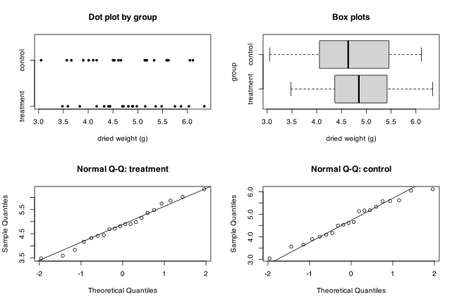
All values lie between \(3.05\) and \(6.34\) g, which is plausible for dried plant material, so there are no obvious data-entry errors. Both distributions are single-peaked and roughly symmetric; the Normal probability plots are close to straight, so the Normality assumption is credible. The two spreads are very similar (\(s_1 = 0.791\), \(s_2 = 0.864\); the variance-ratio test gives \(F_{19,19} = 0.839\), \(p = 0.71\)), which supports the common-\(\sigma^2\) assumption built into both models. The treatment mean exceeds the control mean by only \(4.860 - 4.726 = 0.134\) g, an eighth of a standard deviation, and the two dot plots overlap almost completely. The exploratory analysis therefore suggests any treatment effect is small relative to the plant-to-plant variation, and we should not expect a significant test.
(b) The unpaired t-test. Since the model assumes a common \(\sigma^2\), the pooled-variance (equal-variance) two-sample \(t\)-test is the one that matches it.
t.test(weight ~ group, data = plant, var.equal = TRUE)
	Two Sample t-test

data:  weight by group
t = 0.50985, df = 38, p-value = 0.6131
alternative hypothesis: true difference in means between group treatment and group control is not equal to 0
95 percent confidence interval:
 -0.3965733  0.6635733
sample estimates:
mean in group treatment   mean in group control
                 4.8600                  4.7265
The estimated difference is \(\overline{y}_1 - \overline{y}_2 = 0.1335\) g with \(t = 0.510\) on \(38\) degrees of freedom and \(p = 0.61\): no evidence against \(\mathrm{H}_0\). The 95% confidence interval \((-0.397, 0.664)\) contains zero. Its width matters more than its \(p\)-value: the data are consistent with the enriched environment reducing mean dry weight by up to about \(0.40\) g or raising it by up to about \(0.66\) g. With \(20\) plants per group the experiment simply cannot resolve effects of this size, so “no significant difference” here means “inconclusive”, not “no effect”.
(c) Estimation. Write \(N = 40\) for the total number of observations. Under \(\mathrm{H}_1\) the log-likelihood, with \(\sigma^2\) a known constant as in Example 2.2.2, is \[ \ell_1(\mu_1,\mu_2;\mathbf{y}) = -\tfrac{1}{2}N\log(2\pi\sigma^2) - \frac{1}{2\sigma^2}\sum_{j=1}^{2}\sum_{k=1}^{20}(y_{jk}-\mu_j)^2 . \] The least squares criterion is \[ S_1 = \sum_{j=1}^{2}\sum_{k=1}^{20}(y_{jk}-\mu_j)^2 , \] so \(\ell_1 = -\tfrac{1}{2}N\log(2\pi\sigma^2) - S_1/(2\sigma^2)\) is a strictly decreasing linear function of \(S_1\). Maximizing \(\ell_1\) and minimizing \(S_1\) therefore give the same equations, exactly as for Equations (2.8) and (2.10) in Example 2.2.2. Differentiating, \[ \frac{\partial \ell_1}{\partial \mu_j} = \frac{1}{\sigma^2}\sum_{k=1}^{20}(y_{jk}-\mu_j) = 0 \quad\Longrightarrow\quad \widehat{\mu}_j = \frac{1}{20}\sum_{k=1}^{20} Y_{jk} = \overline{Y}_j , \] for \(j = 1, 2\). The second derivative is \(-20/\sigma^2 < 0\), so this is a maximum of \(\ell_1\) (equivalently \(\partial^2 S_1/\partial\mu_j^2 = 40 > 0\), a minimum of \(S_1\)).
Under \(\mathrm{H}_0\) the single mean \(\mu\) appears in all \(40\) terms, so \[ \frac{\partial \ell_0}{\partial \mu} = \frac{1}{\sigma^2}\sum_{j=1}^{2}\sum_{k=1}^{20}(y_{jk}-\mu) = 0 \quad\Longrightarrow\quad \widehat{\mu} = \frac{1}{40}\sum_{j=1}^{2}\sum_{k=1}^{20} Y_{jk} = \overline{Y}. \] So the maximum likelihood and least squares estimates coincide and are the obvious sample means: numerically \(\widehat{\mu}_1 = 4.8600\), \(\widehat{\mu}_2 = 4.7265\), \(\widehat{\mu} = 4.79325\).
(d) The minimized criteria. Substituting the estimates from (c) back into the criteria gives the minimum values directly: \[ \widehat{S}_1 = \sum_{j=1}^{2}\sum_{k=1}^{20}(Y_{jk}-\widehat{\mu}_j)^2 = \sum\sum (Y_{jk}-\overline{Y}_j)^2, \qquad \widehat{S}_0 = \sum\sum (Y_{jk}-\overline{Y})^2 . \] That these are minima and not merely stationary values follows because \(S_1\) is a positive-definite quadratic in \((\mu_1,\mu_2)\). Explicitly, for any \(\mu_j\), \[ \sum_k (Y_{jk}-\mu_j)^2 = \sum_k (Y_{jk}-\overline{Y}_j)^2 + 20(\overline{Y}_j - \mu_j)^2 \geq \sum_k (Y_{jk}-\overline{Y}_j)^2 , \] the cross-product vanishing because \(\sum_k (Y_{jk}-\overline{Y}_j) = 0\); equality holds only at \(\mu_j = \overline{Y}_j\). The same identity with a single mean over all \(40\) observations gives \(\widehat{S}_0\).
(e) Chi-squared distributions. Two printing slips in the exercise as set should be noted: in the first display the subtracted term is summed over \(j = 1, 2\) (not \(k = 1,\ldots,20\)), and in the third display the term is \(\frac{40}{\sigma^2}(\overline{Y}-\mu)^2\), the sum over \(j\) being spurious. With those corrections the identities are exactly Exercise 1.4(b) applied group-by-group.
Exercise 1.4(b) states that for \(n\) independent \(\mathrm{N}(\mu,\sigma^2)\) variables, \(\sum_i (Y_i-\overline{Y})^2 = \sum_i (Y_i-\mu)^2 - n(\overline{Y}-\mu)^2\). Applying it within group \(j\) with \(n = 20\) and mean \(\mu_j\), then summing over \(j\) and dividing by \(\sigma^2\), \[ \frac{1}{\sigma^2}\widehat{S}_1 = \frac{1}{\sigma^2}\sum_{j=1}^{2}\sum_{k=1}^{20}(Y_{jk}-\mu_j)^2 - \frac{20}{\sigma^2}\sum_{j=1}^{2}(\overline{Y}_j-\mu_j)^2 . \] If \(\mathrm{H}_1\) is true then \((Y_{jk}-\mu_j)/\sigma \sim \mathrm{N}(0,1)\) independently, so the first term is \(\chi^2(40)\); and \(\overline{Y}_j \sim \mathrm{N}(\mu_j, \sigma^2/20)\) independently across \(j\), so \(\sqrt{20}(\overline{Y}_j-\mu_j)/\sigma \sim \mathrm{N}(0,1)\) and the second term is \(\chi^2(2)\). By Exercise 1.4(c) the sample mean and the within-group sum of squares are independent, so \(\widehat{S}_1/\sigma^2\) is independent of the second term. Writing \(\chi^2(40) = \widehat{S}_1/\sigma^2 + \chi^2(2)\) as a sum of two independent terms and comparing moment generating functions gives \[ \frac{1}{\sigma^2}\widehat{S}_1 \sim \chi^2(38), \] which is \(N\) minus the number of parameters estimated, \(40 - 2 = 38\).
Under \(\mathrm{H}_0\) all \(40\) observations have the same mean \(\mu\), so applying Exercise 1.4(b) once with \(n = 40\), \[ \frac{1}{\sigma^2}\widehat{S}_0 = \frac{1}{\sigma^2}\sum_{j=1}^{2}\sum_{k=1}^{20}(Y_{jk}-\mu)^2 - \frac{40}{\sigma^2}(\overline{Y}-\mu)^2 , \] where now the first term is \(\chi^2(40)\) and the second, since \(\overline{Y}\sim \mathrm{N}(\mu,\sigma^2/40)\), is \(\chi^2(1)\) and independent of \(\widehat{S}_0\). Hence \[ \frac{1}{\sigma^2}\widehat{S}_0 \sim \chi^2(39) = \chi^2(40-1). \]
(f) The F-statistic. Repeat the argument of Example 2.2.2. Expanding \(Y_{jk}-\overline{Y} = (Y_{jk}-\overline{Y}_j) + (\overline{Y}_j-\overline{Y})\) and using \(\sum_k (Y_{jk}-\overline{Y}_j) = 0\), \[ \widehat{S}_0 - \widehat{S}_1 = 20\sum_{j=1}^{2}(\overline{Y}_j - \overline{Y})^2 = 10(\overline{Y}_1-\overline{Y}_2)^2 , \] the last step because with equal group sizes \(\overline{Y} = (\overline{Y}_1+\overline{Y}_2)/2\). Under \(\mathrm{H}_0\), \(\overline{Y}_1-\overline{Y}_2 \sim \mathrm{N}(0, \sigma^2/10)\), so \((\widehat{S}_0-\widehat{S}_1)/\sigma^2 \sim \chi^2(1)\), consistent with the general statement \((\widehat{S}_0-\widehat{S}_1)/\sigma^2 \sim \chi^2(J-1)\) in Section 2.2.2 with \(J = 2\). Moreover \(\widehat{S}_0 - \widehat{S}_1\) is a function of the group means alone while \(\widehat{S}_1\) is a function of the within-group deviations alone, and these are independent for Normal data; so the two chi-squared variables are independent. Since \(\sigma^2\) is unknown in practice we eliminate it by taking the ratio of the two independent chi-squared variables, each divided by its degrees of freedom: \[ F = \frac{(\widehat{S}_0-\widehat{S}_1)/\sigma^2}{1} \bigg/ \frac{\widehat{S}_1/\sigma^2}{38} = \frac{\widehat{S}_0-\widehat{S}_1}{\widehat{S}_1/38} \sim F(1,38) \] if \(\mathrm{H}_0\) is true, by the definition of the \(F\)-distribution in Section 1.4.4. If \(\mathrm{H}_0\) is false then \(\mathrm{E}(\overline{Y}_1-\overline{Y}_2) = \mu_1-\mu_2 \neq 0\), so \((\widehat{S}_0-\widehat{S}_1)/\sigma^2\) has a non-central chi-squared distribution with non-centrality parameter \(10(\mu_1-\mu_2)^2/\sigma^2\) and \(F\) has a non-central \(F\)-distribution, shifted to the right of the central one (Figure 2.5).
(g) Testing. Computing the two minima and the statistic directly from their definitions:
y <- plant$weight
S0 <- sum((y - mean(y))^2)
S1 <- sum((y - ave(y, plant$group))^2)
Fstat <- (S0 - S1) / (S1 / 38)
c(S0 = S0, S1 = S1, F = Fstat, p = pf(Fstat, 1, 38, lower.tail = FALSE))
        S0         S1          F          p
26.2316775 26.0534550  0.2599446  0.6131068
The same numbers come out of the model-comparison machinery, which is a useful check that \(\widehat{S}_0\) and \(\widehat{S}_1\) are the residual sums of squares of the two nested linear models:
anova(lm(weight ~ 1, data = plant), lm(weight ~ group, data = plant))
Analysis of Variance Table

Model 1: weight ~ 1
Model 2: weight ~ group
  Res.Df    RSS Df Sum of Sq      F Pr(>F)
1     39 26.232
2     38 26.053  1   0.17822 0.2599 0.6131
Fitting separate group means reduces the sum of squares from \(26.232\) to \(26.053\), an improvement of only \(0.178\), or \(0.7\)% of the total. With \(F = 0.260\) on \((1, 38)\) degrees of freedom, \(p = 0.61\), this is far below the \(95\)th percentile \(F_{0.95}(1,38) = 4.10\). There is no evidence against \(\mathrm{H}_0\); on grounds of simplicity the single-mean model is preferable, and the nutritional enrichment has no demonstrable effect on mean dry weight.
(h) Relation to the t-test. Section 1.4.4 records that if \(T \sim t(n)\) then \(T^2 \sim F(1,n)\). Here \(t = 0.50985\) and \(t^2 = 0.25994 = F\) to five decimal places, and the two \(p\)-values agree exactly at \(0.6131\) because the two-sided \(t\) test and the one-sided upper-tail \(F\) test reject on the same event \(\{|T| > c\}\). The two procedures are algebraically the same test: the least squares comparison of nested models with a one-degree-of-freedom difference is the unpaired \(t\)-test rewritten. The conclusions in (b) and (g) are therefore identical, but the \(t\)-test formulation is more informative in practice because it also delivers the signed estimate and the confidence interval, whereas \(F\) discards the sign of the effect.
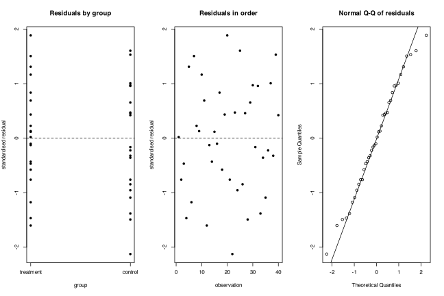
(i) Residuals. Under \(\mathrm{H}_0\) the fitted value for every observation is \(\widehat{\mu} = \overline{y}\), so the raw residuals are \(y_{jk}-\overline{y}\); standardizing by \(s = \sqrt{\widehat{S}_0/39}\) gives residuals comparable with Figures 2.3 and 2.4 of Example 2.2.2.
r <- (y - mean(y)) / sqrt(S0 / 39)
par(mfrow = c(1, 3))
plot(as.integer(plant$group), r, xaxt = "n", xlab = "group",
     ylab = "standardised residual", main = "Residuals by group", pch = 16)
axis(1, at = 1:2, labels = levels(plant$group)); abline(h = 0, lty = 2)
plot(seq_along(r), r, xlab = "observation", ylab = "standardised residual",
     main = "Residuals in order", pch = 16); abline(h = 0, lty = 2)
qqnorm(r, main = "Normal Q-Q of residuals"); qqline(r)
round(c(mean = mean(r), sd = sd(r), min = min(r), max = max(r)), 3)
tapply(r, plant$group, mean)
shapiro.test(r)
  mean     sd    min    max
 0.000  1.000 -2.126  1.886

 treatment    control
 0.0813899 -0.0813899

	Shapiro-Wilk normality test

data:  r
W = 0.9844, p-value = 0.8457
The residuals have mean zero and unit standard deviation by construction. The Normal probability plot is close to a straight line and no residual lies beyond \(\pm 2.13\), well inside what \(40\) standard Normal draws would produce; the Shapiro-Wilk test gives \(p = 0.85\). The spread is visually the same in the two groups, supporting the constant-variance assumption. Crucially the residuals show no group structure: the two group means of the residuals are \(+0.081\) and \(-0.081\), tiny compared with a residual standard deviation of \(1\). That is the diagnostic restatement of (g) — the omitted group term would explain almost none of the residual variation, so the \(\mathrm{H}_0\) model is adequate for these data.
Problem 2.2 — The weights, in kilograms, of twenty men before and after participation
The weights, in kilograms, of twenty men before and after participation in a “waist loss” program are shown in Table 2.8 (Egger et al. 1999). We want to know if, on average, they retain a weight loss twelve months after the program.
Table 2.8 (Weights of twenty men before and after participation in a “waist loss” program) lists, as (man, before, after): \((1, 100.8, 97.0)\), \((2, 102.0, 107.5)\), \((3, 105.9, 97.0)\), \((4, 108.0, 108.0)\), \((5, 92.0, 84.0)\), \((6, 116.7, 111.5)\), \((7, 110.2, 102.5)\), \((8, 135.0, 127.5)\), \((9, 123.5, 118.5)\), \((10, 95.0, 94.2)\), \((11, 105.0, 105.0)\), \((12, 85.0, 82.4)\), \((13, 107.2, 98.2)\), \((14, 80.0, 83.6)\), \((15, 115.1, 115.0)\), \((16, 103.5, 103.0)\), \((17, 82.0, 80.0)\), \((18, 101.5, 101.5)\), \((19, 103.5, 102.6)\), \((20, 93.0, 93.0)\).
Let \(Y_{jk}\) denote the weight of the \(k\)th man at the \(j\)th time, where \(j = 1\) before the program and \(j = 2\) twelve months later. Assume the \(Y_{jk}\)’s are independent random variables with \(Y_{jk} \sim \mathrm{N}(\mu_j, \sigma^2)\) for \(j = 1, 2\) and \(k = 1, \ldots, 20\).
- a.
- Use an unpaired \(t\)-test to test the hypothesis \[ \mathrm{H}_0 : \mu_1 = \mu_2 \qquad \text{versus} \qquad \mathrm{H}_1 : \mu_1 \neq \mu_2 . \]
- b.
- Let \(D_k = Y_{1k} - Y_{2k}\), for \(k = 1, \ldots, 20\). Formulate models for testing \(\mathrm{H}_0\) against \(\mathrm{H}_1\) using the \(D_k\)’s. Using analogous methods to Exercise 2.1 above, assuming \(\sigma^2\) is a known constant, test \(\mathrm{H}_0\) against \(\mathrm{H}_1\).
- c.
- The analysis in (b) is a paired \(t\)-test which uses the natural relationship between weights of the same person before and after the program. Are the conclusions the same from (a) and (b)?
- d.
- List the assumptions made for (a) and (b). Which analysis is more appropriate for these data?
(difficulty: \(\star\star\))
The data ship in the dobson package as waist, one row per man with columns before and after.
library(dobson)
data(waist)
w <- data.frame(weight = c(waist$before, waist$after),
                time = factor(rep(c("before", "after"), each = 20),
                              levels = c("before", "after")))
round(t(sapply(split(w$weight, w$time),
       function(v) c(n = length(v), mean = mean(v), sd = sd(v),
                     min = min(v), max = max(v)))), 3)
        n    mean     sd min   max
before 20 103.245 13.517  80 135.0
after  20 100.600 12.475  80 127.5
d <- waist$before - waist$after
par(mfrow = c(1, 3))
plot(waist$before, waist$after, pch = 16, xlab = "weight before (kg)",
     ylab = "weight after (kg)", main = "Paired weights")
abline(0, 1, lty = 2)
stripchart(d, method = "stack", pch = 16,
           xlab = "difference before - after (kg)",
           main = "Individual weight losses")
abline(v = 0, lty = 2)
qqnorm(d, main = "Normal Q-Q of differences"); qqline(d)
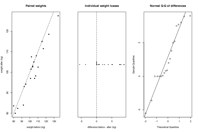
The scatter plot is the whole story: the points lie almost on the line \(y = x\), and nearly all of them sit just below it. The men differ enormously from each other (weights run from \(80\) to \(135\) kg), but each man changes only a little.
(a) The unpaired t-test. Treating the two sets of \(20\) weights as independent samples, as the exercise’s stated model does:
t.test(weight ~ time, data = w, var.equal = TRUE)
	Two Sample t-test

data:  weight by time
t = 0.64309, df = 38, p-value = 0.524
alternative hypothesis: true difference in means between group before and group after is not equal to 0
95 percent confidence interval:
 -5.68128 10.97128
sample estimates:
mean in group before  mean in group after
             103.245              100.600
The estimated mean loss is \(103.245 - 100.600 = 2.645\) kg, but \(t = 0.643\) on \(38\) degrees of freedom gives \(p = 0.52\) and the 95% confidence interval \((-5.68, 10.97)\) is very wide. On this analysis there is no evidence of a retained weight loss.
(b) The paired analysis. Work with the \(20\) differences \(D_k = Y_{1k} - Y_{2k}\). Under the stated assumptions \(D_k \sim \mathrm{N}(\delta, \sigma_D^2)\) with \(\delta = \mu_1 - \mu_2\), and the \(D_k\) are independent across men. The two competing models are \[ \mathrm{H}_0 : \mathrm{E}(D_k) = 0; \quad D_k \sim \mathrm{N}(0,\sigma_D^2), \qquad \mathrm{H}_1 : \mathrm{E}(D_k) = \delta; \quad D_k \sim \mathrm{N}(\delta,\sigma_D^2), \] for \(k = 1,\ldots,20\), with \(\sigma_D^2\) treated as a known constant. Exactly as in Exercise 2.1(c), maximizing the log-likelihood \[ \ell_1(\delta;\mathbf{d}) = -\tfrac{1}{2}\cdot 20\log(2\pi\sigma_D^2) - \frac{1}{2\sigma_D^2}\sum_{k=1}^{20}(d_k-\delta)^2 \] is equivalent to minimizing \(S_1 = \sum_k (d_k-\delta)^2\), and gives \(\widehat{\delta} = \overline{D}\). The minimized criteria are \[ \widehat{S}_0 = \sum_{k=1}^{20} D_k^2 \quad (\text{no parameters estimated}), \qquad \widehat{S}_1 = \sum_{k=1}^{20}(D_k-\overline{D})^2 \quad (\text{one parameter}). \] By Exercise 1.4(b) with \(n = 20\), \(\widehat{S}_1/\sigma_D^2 = \sum_k (D_k-\delta)^2/\sigma_D^2 - 20(\overline{D}-\delta)^2/\sigma_D^2\), a \(\chi^2(20)\) minus an independent \(\chi^2(1)\), so \(\widehat{S}_1/\sigma_D^2 \sim \chi^2(19)\) whether or not \(\mathrm{H}_0\) holds. If \(\mathrm{H}_0\) is true then \(\widehat{S}_0/\sigma_D^2 \sim \chi^2(20)\) and \(\widehat{S}_0 - \widehat{S}_1 = 20\overline{D}^2\) with \(\overline{D} \sim \mathrm{N}(0,\sigma_D^2/20)\), so \((\widehat{S}_0-\widehat{S}_1)/\sigma_D^2 \sim \chi^2(1)\) independently of \(\widehat{S}_1\). Hence \[ F = \frac{\widehat{S}_0-\widehat{S}_1}{\widehat{S}_1/19} \sim F(1,19) \quad \text{if } \mathrm{H}_0 \text{ is true.} \]
S0 <- sum(d^2); S1 <- sum((d - mean(d))^2)
Fstat <- (S0 - S1) / (S1 / 19)
c(S0 = S0, S1 = S1, diff = S0 - S1, F = Fstat,
  p = pf(Fstat, 1, 19, lower.tail = FALSE))
          S0           S1         diff            F            p
4.619100e+02 3.219895e+02 1.399205e+02 8.256448e+00 9.730463e-03
\(F = 8.256\) on \((1,19)\) degrees of freedom gives \(p = 0.0097\), well beyond the \(95\)th percentile \(F_{0.95}(1,19) = 4.38\), so \(\mathrm{H}_0\) is rejected. Equivalently, as a \(t\)-statistic:
t.test(waist$before, waist$after, paired = TRUE)
	Paired t-test

data:  waist$before and waist$after
t = 2.8734, df = 19, p-value = 0.00973
alternative hypothesis: true mean difference is not equal to 0
95 percent confidence interval:
 0.718348 4.571652
sample estimates:
mean difference
          2.645
Note \(t^2 = 2.8734^2 = 8.256 = F\), the same \(t\)-versus-\(F\) identity used in Exercise 2.1(h). On average the men retain a loss of \(2.645\) kg twelve months on, with 95% confidence interval \((0.72, 4.57)\) kg.
(c) Comparison. No — the conclusions are opposite. Both analyses estimate the same quantity, \(2.645\) kg, but the unpaired analysis attaches a standard error of \(4.11\) kg to it while the paired analysis attaches \(0.92\) kg, a four-and-a-half-fold reduction. The reason is the correlation between a man’s two weights:
c(cor = cor(waist$before, waist$after),
  se_unpaired = sqrt(var(waist$before)/20 + var(waist$after)/20),
  se_paired = sd(d)/sqrt(20))
      cor se_unpaired   se_paired
0.9529734   4.1129735   0.9205112
With \(\mathrm{corr}(Y_{1k},Y_{2k}) = \rho = 0.953\), \(\mathrm{var}(D_k) = 2\sigma^2(1-\rho)\) is only about \(5\)% of the \(2\sigma^2\) the unpaired analysis assumes. Pairing removes the between-man variation — which is the dominant source of scatter and is irrelevant to the question — and leaves only the within-man change. The unpaired test is not wrong arithmetically; it is answering the question with the wrong yardstick, and its failure to reject is a Type II error.
(d) Assumptions. Assumptions for (a): the \(40\) observations are mutually independent; both sets are Normally distributed; the two variances are equal; the sample is representative of the population of interest. The independence assumption is the fatal one, since the same \(20\) men are measured twice.
Assumptions for (b): the \(20\) differences \(D_k\) are mutually independent (reasonable — different men); each \(D_k\) is Normal with common variance \(\sigma_D^2\) (the Q-Q plot above is acceptably straight, Shapiro-Wilk \(p = 0.16\), though there are several exact zeros where a man’s weight was recorded unchanged); and the \(D_k\) share a common mean \(\delta\), i.e. the retained loss does not depend on initial weight. Nothing is assumed about the between-man distribution of weights, and no equal-variance assumption across times is needed.
shapiro.test(d)
summary(lm(d ~ waist$before))$coefficients
	Shapiro-Wilk normality test

data:  d
W = 0.93148, p-value = 0.1649

               Estimate Std. Error   t value   Pr(>|t|)
(Intercept)  -9.8004283  6.8611113 -1.428402 0.17029887
waist$before  0.1205427  0.0659201  1.828618 0.08407696
Regressing the loss on initial weight gives a slope of \(0.121\) kg per kg of initial weight, \(p = 0.084\): a heavier man tends to retain a slightly larger loss, but the evidence is weak and the common-\(\delta\) assumption is not clearly contradicted. This is worth flagging rather than acting on with \(n = 20\).
The paired analysis in (b) is the appropriate one. The design is a before-and-after study on the same subjects, so the data are paired by construction and the independence assumed in (a) does not hold. Conclusion: twelve months after the program the men retain a mean weight loss of about \(2.6\) kg (95% CI \(0.7\) to \(4.6\) kg). Two caveats on interpretation remain, neither statistical: there is no control group, so regression to the mean and secular trends cannot be separated from the program effect; and the individual results are heterogeneous — \(14\) men lost weight, \(4\) were unchanged to the recorded precision, and \(2\) gained.
Problem 2.3 — For Model (2.7) for the data on birthweight and gestational age, using
For Model (2.7) for the data on birthweight and gestational age, using methods similar to those for Exercise 1.4, show \[ \widehat{S}_1 = \sum_{j=1}^{J}\sum_{k=1}^{K}(Y_{jk}-a_j-b_j x_{jk})^2 \] \[ = \sum_{j=1}^{J}\sum_{k=1}^{K}\left[Y_{jk}-(\alpha_j+\beta_j x_{jk})\right]^2 - K\sum_{j=1}^{J}(\overline{Y}_j - \alpha_j - \beta_j \overline{x}_j)^2 \] \[ \phantom{=} - \sum_{j=1}^{J}(b_j-\beta_j)^2\left(\sum_{k=1}^{K}x_{jk}^2 - K\overline{x}_j^2\right) \] and that the random variables \(Y_{jk}\), \(\overline{Y}_j\) and \(b_j\) are all independent and have the following distributions \[ Y_{jk} \sim \mathrm{N}(\alpha_j+\beta_j x_{jk}, \sigma^2), \] \[ \overline{Y}_j \sim \mathrm{N}(\alpha_j+\beta_j \overline{x}_j, \sigma^2/K), \] \[ b_j \sim \mathrm{N}\!\left(\beta_j,\ \sigma^2\Big/\Big(\sum_{k=1}^{K}x_{jk}^2 - K\overline{x}_j^2\Big)\right). \]
Here Model (2.7) is \(\mathrm{E}(Y_{jk}) = \mu_{jk} = \alpha_j + \beta_j x_{jk}\) with \(Y_{jk} \sim \mathrm{N}(\mu_{jk},\sigma^2)\) independent, \(j = 1,\ldots,J\) indexing the groups (boys and girls, so \(J = 2\)) and \(k = 1,\ldots,K\) the babies within a group (\(K = 12\)); \(a_j\) and \(b_j\) are the least squares estimates of \(\alpha_j\) and \(\beta_j\) given in Section 2.2.2 by \(b_j = \left(K\sum_k x_{jk}Y_{jk} - (\sum_k x_{jk})(\sum_k Y_{jk})\right)/\left(K\sum_k x_{jk}^2 - (\sum_k x_{jk})^2\right)\) and \(a_j = \overline{Y}_j - b_j\overline{x}_j\).
(difficulty: \(\star\star\star\))
Throughout, fix a group \(j\) and write \[ S_{xx} = \sum_{k=1}^{K}(x_{jk}-\overline{x}_j)^2 = \sum_{k=1}^{K}x_{jk}^2 - K\overline{x}_j^2, \qquad S_{xY} = \sum_{k=1}^{K}(x_{jk}-\overline{x}_j)(Y_{jk}-\overline{Y}_j), \] \[ S_{YY} = \sum_{k=1}^{K}(Y_{jk}-\overline{Y}_j)^2 , \] so that the least squares estimates of Section 2.2.2 are \(b_j = S_{xY}/S_{xx}\) and \(a_j = \overline{Y}_j - b_j\overline{x}_j\). Assume \(S_{xx} > 0\), i.e. the gestational ages within a group are not all equal.
(1) The algebraic identity. Substituting \(a_j = \overline{Y}_j - b_j\overline{x}_j\) removes the intercept: \[ Y_{jk}-a_j-b_j x_{jk} = (Y_{jk}-\overline{Y}_j) - b_j(x_{jk}-\overline{x}_j), \] whence the group-\(j\) contribution to \(\widehat{S}_1\) is \[ \widehat{S}_{1j} = S_{YY} - 2b_j S_{xY} + b_j^2 S_{xx} = S_{YY} - b_j^2 S_{xx}, \tag{i} \] using \(S_{xY} = b_j S_{xx}\) twice.
Now work on the right-hand side. Put \(e_{jk} = Y_{jk} - (\alpha_j + \beta_j x_{jk})\), so that \(\overline{e}_j = \overline{Y}_j - \alpha_j - \beta_j\overline{x}_j\) is precisely the quantity squared in the second term. Exercise 1.4(b), applied to \(e_{j1},\ldots,e_{jK}\) with \(n = K\), gives \[ \sum_{k}e_{jk}^2 - K\overline{e}_j^2 = \sum_k (e_{jk}-\overline{e}_j)^2 . \] Since \(e_{jk}-\overline{e}_j = (Y_{jk}-\overline{Y}_j) - \beta_j(x_{jk}-\overline{x}_j)\), \[ \sum_k (e_{jk}-\overline{e}_j)^2 = S_{YY} - 2\beta_j S_{xY} + \beta_j^2 S_{xx} = S_{YY} - 2\beta_j b_j S_{xx} + \beta_j^2 S_{xx}. \] Subtracting the third term, and expanding \((b_j-\beta_j)^2 S_{xx} = b_j^2 S_{xx} - 2b_j\beta_j S_{xx} + \beta_j^2 S_{xx}\), everything involving \(\beta_j\) cancels: \[ \sum_k e_{jk}^2 - K\overline{e}_j^2 - (b_j-\beta_j)^2 S_{xx} = S_{YY} - b_j^2 S_{xx} = \widehat{S}_{1j} \] by (i). Summing over \(j = 1,\ldots,J\) gives the stated identity. Note it is an algebraic identity: it holds for any numbers \(\alpha_j,\beta_j\), not only the true parameter values. A numerical check on the birthweight data, using both the true-ish fitted values from Table 2.5 and a pair of arbitrary values, confirms this:
library(dobson)
data(birthweight)
bw <- data.frame(y   = c(birthweight[[2]], birthweight[[4]]),
                 x   = c(birthweight[[1]], birthweight[[3]]),
                 sex = rep(c("boys", "girls"), each = 12))
K <- 12
check <- function(alpha, beta) {
  S1 <- 0; A <- 0; B <- 0; C <- 0
  for (j in unique(bw$sex)) {
    yj <- bw$y[bw$sex == j]; xj <- bw$x[bw$sex == j]
    i  <- match(j, unique(bw$sex))
    bj <- cov(xj, yj) / var(xj); aj <- mean(yj) - bj * mean(xj)
    Sxx <- sum(xj^2) - K * mean(xj)^2
    S1 <- S1 + sum((yj - aj - bj * xj)^2)
    A  <- A + sum((yj - (alpha[i] + beta[i] * xj))^2)
    B  <- B + K * (mean(yj) - alpha[i] - beta[i] * mean(xj))^2
    C  <- C + (bj - beta[i])^2 * Sxx
  }
  c(S1 = S1, rhs = A - B - C, A = A, B = B, C = C)
}
round(check(c(-1268.672, -2141.667), c(111.983, 130.400)), 4)
round(check(c(0, 500), c(100, 90)), 4)
         S1         rhs           A           B           C
652424.5218 652424.5218 652424.5230      0.0011      0.0000

         S1         rhs           A           B           C
  652424.52   652424.52 22475004.00 21757861.67    64717.81
The value \(\widehat{S}_1 = 652424.5\) agrees with Table 2.5, and rhs reproduces it in both cases even though the three components differ by orders of magnitude.
(2) The distributions. \(Y_{jk} \sim \mathrm{N}(\alpha_j+\beta_j x_{jk},\sigma^2)\) is the model assumption in (2.7) itself. Both \(\overline{Y}_j\) and \(b_j\) are linear combinations of independent Normal variables, hence Normal, and it remains to compute the two moments in each case. For the mean, \[ \mathrm{E}(\overline{Y}_j) = \frac{1}{K}\sum_k (\alpha_j+\beta_j x_{jk}) = \alpha_j + \beta_j \overline{x}_j, \qquad \mathrm{var}(\overline{Y}_j) = \frac{1}{K^2}\sum_k \sigma^2 = \frac{\sigma^2}{K}. \] For the slope, write it in the equivalent centred form \[ b_j = \frac{S_{xY}}{S_{xx}} = \frac{1}{S_{xx}}\sum_k (x_{jk}-\overline{x}_j)Y_{jk}, \] the replacement of \(Y_{jk}-\overline{Y}_j\) by \(Y_{jk}\) being legitimate because \(\sum_k (x_{jk}-\overline{x}_j) = 0\). Then, using \(\sum_k (x_{jk}-\overline{x}_j)x_{jk} = S_{xx}\), \[ \mathrm{E}(b_j) = \frac{1}{S_{xx}}\sum_k (x_{jk}-\overline{x}_j)(\alpha_j+\beta_j x_{jk}) = \frac{\beta_j S_{xx}}{S_{xx}} = \beta_j , \] \[ \mathrm{var}(b_j) = \frac{\sigma^2}{S_{xx}^2}\sum_k (x_{jk}-\overline{x}_j)^2 = \frac{\sigma^2}{S_{xx}} = \frac{\sigma^2}{\sum_k x_{jk}^2 - K\overline{x}_j^2}, \] as required.
(3) The independence. The exercise’s phrase “the random variables \(Y_{jk}\), \(\overline{Y}_j\) and \(b_j\) are all independent” cannot be taken literally, since \(\overline{Y}_j\) is a function of the \(Y_{jk}\) in its own group. What the degrees-of-freedom argument of Section 2.2.2 actually needs, and what is true, is that within each group the three terms of the decomposition are mutually independent; across groups everything is independent because the groups involve disjoint sets of \(Y_{jk}\).
Rearranged, the identity reads \[ \frac{1}{\sigma^2}\sum_j\sum_k e_{jk}^2 = \frac{\widehat{S}_1}{\sigma^2} + \frac{K}{\sigma^2}\sum_j \overline{e}_j^2 + \frac{1}{\sigma^2}\sum_j (b_j-\beta_j)^2 S_{xx,j}. \] Fix \(j\) and regard \(\mathbf{e}_j = (e_{j1},\ldots,e_{jK})^{\mathrm{T}} \sim \mathrm{N}_K(\mathbf{0},\sigma^2 \mathbf{I})\). Let \(V_j\) be the two-dimensional subspace of \(\mathbb{R}^K\) spanned by the orthogonal vectors \(\mathbf{u}_1 = \mathbf{1}/\sqrt{K}\) and \(\mathbf{u}_2 = (\mathbf{x}_j - \overline{x}_j\mathbf{1})/\sqrt{S_{xx}}\). Then \[ \mathbf{u}_1^{\mathrm{T}}\mathbf{e}_j = \sqrt{K}\,\overline{e}_j, \qquad \mathbf{u}_2^{\mathrm{T}}\mathbf{e}_j = \frac{S_{xY}-\beta_j S_{xx}}{\sqrt{S_{xx}}} = (b_j-\beta_j)\sqrt{S_{xx}}, \] so the three terms of the decomposition are exactly \(\|(\mathbf{I}-\mathbf{P}_j)\mathbf{e}_j\|^2\), \((\mathbf{u}_1^{\mathrm{T}}\mathbf{e}_j)^2\) and \((\mathbf{u}_2^{\mathrm{T}}\mathbf{e}_j)^2\), where \(\mathbf{P}_j\) projects onto \(V_j\). Because \(\mathbf{e}_j\) is spherically Normal, its components along mutually orthogonal directions — and its component in the orthogonal complement — are independent. Dividing by \(\sigma^2\), \[ \frac{\widehat{S}_{1j}}{\sigma^2}\sim\chi^2(K-2), \qquad \frac{K\overline{e}_j^2}{\sigma^2}\sim\chi^2(1), \qquad \frac{(b_j-\beta_j)^2 S_{xx}}{\sigma^2}\sim\chi^2(1), \] independently, and these add to \(\chi^2(K)\) as they must. In particular \(\overline{Y}_j\) and \(b_j\) are uncorrelated, \[ \mathrm{cov}(\overline{Y}_j, b_j) = \frac{\sigma^2}{K S_{xx}}\sum_k (x_{jk}-\overline{x}_j) = 0, \] and jointly Normal, hence independent — which is the substantive content of the exercise’s claim. Summing the independent contributions over \(j = 1,\ldots,J\) gives \(\widehat{S}_1/\sigma^2 \sim \chi^2(JK-2J)\), the result quoted in Section 2.2.2, the degrees of freedom being the number of observations \(JK\) minus the number of parameters estimated, \(2J\).
Problem 2.4 — Suppose you have the following data
Suppose you have the following data
| \(x\) | 1.0 | 1.2 | 1.4 | 1.6 | 1.8 | 2.0 |
|---|---|---|---|---|---|---|
| \(y\) | 3.15 | 4.85 | 6.50 | 7.20 | 8.25 | 16.50 |
and you want to fit a model with \[ \mathrm{E}(Y) = \ln(\beta_0 + \beta_1 x + \beta_2 x^2). \] Write this model in the form of (2.13) specifying the vectors \(\mathbf{y}\) and \(\boldsymbol{\beta}\) and the matrix \(\mathbf{X}\).
Equation (2.13) of Section 2.4 is \(g[\mathrm{E}(\mathbf{y})] = \mathbf{X}\boldsymbol{\beta}\), where \(\mathbf{y}\) is the \(N \times 1\) vector of responses, \(g[\mathrm{E}(\mathbf{y})]\) denotes the vector with elements \(g[\mathrm{E}(Y_i)]\) for a single link function \(g\), \(\boldsymbol{\beta}\) is the \(p \times 1\) vector of parameters and \(\mathbf{X}\) is the \(N \times p\) design matrix.
(difficulty: \(\star\))
The task is to identify the link. The mean is given as a function of the linear component rather than the other way round, so invert it: applying \(\exp\) to both sides of \(\mathrm{E}(Y_i) = \ln(\beta_0+\beta_1 x_i+\beta_2 x_i^2)\) gives \[ \exp[\mathrm{E}(Y_i)] = \beta_0 + \beta_1 x_i + \beta_2 x_i^2 . \] This is of the form \(g[\mathrm{E}(Y_i)] = \beta_0 + \beta_1 x_{i1} + \beta_2 x_{i2}\) required by Section 2.4, with link function \[ g(\mu) = e^{\mu} \] and with two explanatory terms \(x_{i1} = x_i\) and \(x_{i2} = x_i^2\). Note that although the model is quadratic in \(x\), it is still linear in the parameters, which is all that (2.13) requires: \(x\) and \(x^2\) are simply two columns of measured constants.
There are \(N = 6\) observations and \(p = 3\) parameters, so \[ \mathbf{y} = \begin{bmatrix} 3.15 \\ 4.85 \\ 6.50 \\ 7.20 \\ 8.25 \\ 16.50 \end{bmatrix}, \qquad \boldsymbol{\beta} = \begin{bmatrix} \beta_0 \\ \beta_1 \\ \beta_2 \end{bmatrix}, \qquad \mathbf{X} = \begin{bmatrix} 1 & 1.0 & 1.00 \\ 1 & 1.2 & 1.44 \\ 1 & 1.4 & 1.96 \\ 1 & 1.6 & 2.56 \\ 1 & 1.8 & 3.24 \\ 1 & 2.0 & 4.00 \end{bmatrix}, \] and the model in the form of (2.13) is \[ g[\mathrm{E}(\mathbf{y})] = \begin{bmatrix} \exp[\mathrm{E}(Y_1)] \\ \vdots \\ \exp[\mathrm{E}(Y_6)] \end{bmatrix} = \mathbf{X}\boldsymbol{\beta}. \]
The design matrix is just a Vandermonde-style construction:
x <- c(1.0, 1.2, 1.4, 1.6, 1.8, 2.0)
y <- c(3.15, 4.85, 6.50, 7.20, 8.25, 16.50)
X <- cbind(1, x, x^2)
colnames(X) <- c("beta0", "beta1", "beta2")
X
     beta0 beta1 beta2
[1,]     1   1.0  1.00
[2,]     1   1.2  1.44
[3,]     1   1.4  1.96
[4,]     1   1.6  2.56
[5,]     1   1.8  3.24
[6,]     1   2.0  4.00
Two remarks that the exercise does not ask for but that matter if the model is ever fitted. First, the parameter space is restricted: the logarithm requires \(\beta_0+\beta_1 x+\beta_2 x^2 > 0\) over the range of \(x\), so unlike an ordinary linear model \(\boldsymbol{\beta}\) is not free to roam \(\mathbb{R}^3\). Second, this link makes the fit numerically awkward here, because \(\exp(y)\) ranges from \(\exp(3.15) \approx 23\) to \(\exp(16.5) \approx 1.5\times 10^7\) and a quadratic cannot follow that. Fitting by least squares with a custom link confirms it:
explink <- structure(list(
  linkfun  = function(mu)  exp(mu),
  linkinv  = function(eta) log(pmax(eta, .Machine$double.eps)),
  mu.eta   = function(eta) 1 / pmax(eta, .Machine$double.eps),
  valideta = function(eta) all(eta > 0),
  name     = "exp"), class = "link-glm")
fit <- glm(y ~ x + I(x^2), family = gaussian(link = explink),
           start = c(exp(3), 1, 1))
round(coef(fit), 2)
round(cbind(y = y, fitted = fitted(fit)), 3)
(Intercept)           x      I(x^2)
   60843.03  -111879.21    51059.77

      y fitted
1  3.15  3.161
2  4.85  4.737
3  6.50  8.364
4  7.20  9.437
5  8.25 10.122
6 16.50 10.629
The residual sum of squares is \(46.47\), and a multi-start Nelder-Mead search over the constrained parameter space finds no better optimum, so this is the least squares solution rather than a convergence failure. It is simply a bad fit: the last observation \(y = 16.50\) is far above what the model can reach. The exercise is about notation, but it also illustrates that writing a model in the form of (2.13) says nothing about whether that model suits the data.
Problem 2.5 — The model for two-factor analysis of variance with two levels of one factor,
The model for two-factor analysis of variance with two levels of one factor, three levels of the other and no replication is \[ \mathrm{E}(Y_{jk}) = \mu_{jk} = \mu + \alpha_j + \beta_k; \qquad Y_{jk} \sim \mathrm{N}(\mu_{jk},\sigma^2), \] where \(j = 1, 2\); \(k = 1, 2, 3\) and, using the sum-to-zero constraints, \(\alpha_1 + \alpha_2 = 0\), \(\beta_1 + \beta_2 + \beta_3 = 0\). Also the \(Y_{jk}\)’s are assumed to be independent. Write the equation for \(\mathrm{E}(Y_{jk})\) in matrix notation. (Hint: Let \(\alpha_2 = -\alpha_1\), and \(\beta_3 = -\beta_1 - \beta_2\).)
(difficulty: \(\star\))
There are \(N = 6\) observations but the unconstrained expression \(\mu+\alpha_j+\beta_k\) carries \(1+2+3 = 6\) parameters, and they are not all identifiable: adding a constant to \(\mu\) and subtracting it from every \(\alpha_j\) leaves all six means unchanged. This is the situation flagged in Example 2.4.3(b) — “too many parameters” — and the sum-to-zero constraints of Example 2.4.3(d) are the fix. They remove one parameter from each factor, leaving \(p = 4\) free parameters \[ \boldsymbol{\beta} = \begin{bmatrix} \mu \\ \alpha_1 \\ \beta_1 \\ \beta_2 \end{bmatrix}. \]
Following the hint, substitute \(\alpha_2 = -\alpha_1\) and \(\beta_3 = -\beta_1-\beta_2\) into the six means: \[ \mathrm{E}(Y_{11}) = \mu+\alpha_1+\beta_1, \qquad \mathrm{E}(Y_{12}) = \mu+\alpha_1+\beta_2, \qquad \mathrm{E}(Y_{13}) = \mu+\alpha_1-\beta_1-\beta_2, \] \[ \mathrm{E}(Y_{21}) = \mu-\alpha_1+\beta_1, \qquad \mathrm{E}(Y_{22}) = \mu-\alpha_1+\beta_2, \qquad \mathrm{E}(Y_{23}) = \mu-\alpha_1-\beta_1-\beta_2 . \] Reading off the coefficients of \((\mu,\alpha_1,\beta_1,\beta_2)\) row by row gives the model in the form of (2.13), with \(g\) the identity function: \[ \mathrm{E}(\mathbf{y}) = \mathbf{X}\boldsymbol{\beta}, \qquad \mathbf{y} = \begin{bmatrix} Y_{11} \\ Y_{12} \\ Y_{13} \\ Y_{21} \\ Y_{22} \\ Y_{23} \end{bmatrix}, \qquad \mathbf{X} = \begin{bmatrix} 1 & 1 & 1 & 0 \\ 1 & 1 & 0 & 1 \\ 1 & 1 & -1 & -1 \\ 1 & -1 & 1 & 0 \\ 1 & -1 & 0 & 1 \\ 1 & -1 & -1 & -1 \end{bmatrix}. \]
The second column is the sum-to-zero (effect) coding for the two-level factor, exactly the rows \([\,1\ \ 1\,]\) and \([\,1\ \ -1\,]\) of Example 2.4.3(d) repeated three times each; the last two columns are the corresponding coding for the three-level factor, with the third level coded as minus the sum of the other two so that the level effects sum to zero.
This is what R produces with contr.sum applied to both factors:
d <- expand.grid(k = factor(1:3), j = factor(1:2))
d <- d[order(d$j, d$k), ]
X <- model.matrix(~ j + k, data = d,
                  contrasts.arg = list(j = "contr.sum", k = "contr.sum"))
colnames(X) <- c("mu", "alpha1", "beta1", "beta2")
rownames(X) <- paste0("Y", d$j, d$k)
X[, ]
c(rank = qr(X)$rank, ncol = ncol(X))
    mu alpha1 beta1 beta2
Y11  1      1     1     0
Y12  1      1     0     1
Y13  1      1    -1    -1
Y21  1     -1     1     0
Y22  1     -1     0     1
Y23  1     -1    -1    -1

rank ncol
   4    4
\(\mathbf{X}\) has full column rank \(4\), so the four parameters are estimable — which the unconstrained six-parameter version was not. With \(N = 6\) observations and \(p = 4\) parameters only \(2\) degrees of freedom remain for estimating \(\sigma^2\), the price of having no replication; and because there is no replication no interaction term can be included, since a \(j \times k\) interaction would use up exactly those remaining \(2\) degrees of freedom and leave nothing to estimate the error variance with.
Finally, the design is balanced and the two factors are orthogonal to each other and to the intercept:
t(X) %*% X
       mu alpha1 beta1 beta2
mu      6      0     0     0
alpha1  0      6     0     0
beta1   0      0     4     2
beta2   0      0     2     4
The block-diagonal structure of \(\mathbf{X}^{\mathrm{T}}\mathbf{X}\) means \(\widehat{\mu}\), \(\widehat{\alpha}_1\) and the pair \((\widehat{\beta}_1,\widehat{\beta}_2)\) are mutually uncorrelated, so the estimated effect of one factor does not change when the other factor is added to or dropped from the model. The off-diagonal \(2\) in the lower block is not a defect of the design: it reflects only that the two columns coding a three-level factor cannot both be orthogonal to each other under the sum-to-zero parameterization.
Exponential Family and Generalized Linear Models
Problem 3.1 — The following associations can be described by generalized linear models.
The following associations can be described by generalized linear models. For each one, identify the response variable and the explanatory variables, select a probability distribution for the response (justifying your choice) and write down the linear component.
a. The effect of age, sex, height, mean daily food intake and mean daily energy expenditure on a person’s weight.
b. The proportions of laboratory mice that became infected after exposure to bacteria when five different exposure levels are used and 20 mice are exposed at each level.
c. The association between the number of trips per week to the supermarket for a household and the number of people in the household, the household income and the distance to the supermarket. (difficulty: \(\star\))
Each part is answered with the three components of a generalized linear model set out in Section 3.4: the response distribution from the exponential family, the linear component \(\mathbf{x}_i^T\boldsymbol\beta\), and the link \(g\) with \(g(\mu_i)=\mathbf{x}_i^T\boldsymbol\beta\).
Part (a). The response is \(Y_i\), the weight (kg) of person \(i\). Weight is a continuous measurement, roughly symmetric within a homogeneous group and with no hard upper bound, so \(Y_i \sim N(\mu_i,\sigma^2)\) is the natural first choice; the Normal is in the exponential family (Section 3.2.2) and gives the normal linear model of Section 3.5.1 with the identity link.
The explanatory variables are \(x_{i1}\) age (years), \(x_{i2}\) sex (a dummy, \(1\) for male and \(0\) for female), \(x_{i3}\) height (cm), \(x_{i4}\) mean daily food intake (kJ) and \(x_{i5}\) mean daily energy expenditure (kJ). The linear component is \[ \mathbf{x}_i^T\boldsymbol\beta = \beta_1 + \beta_2 x_{i1} + \beta_3 x_{i2} + \beta_4 x_{i3} + \beta_5 x_{i4} + \beta_6 x_{i5}, \qquad g(\mu_i)=\mu_i . \] Two remarks. Weight is strictly positive and right-skewed in the general population; if the fitted model produced negative predictions or funnel-shaped residuals one would move to \(\log(\text{weight})\) as the response, or to a Gamma distribution with a log link, which keeps \(\mu_i>0\). Also, intake and expenditure enter as a balance, so in practice one would consider the single covariate \(x_{i4}-x_{i5}\).
Part (b). Here the mice at a given exposure level form a set of \(n=20\) independent binary trials with a common infection probability, so the response is \(Y_i\), the number infected out of \(n_i = 20\) at exposure level \(i\) (\(i=1,\dots,5\)), and \(Y_i \sim \mathrm{Bin}(20,\pi_i)\). The Binomial is in the exponential family with natural parameter \(\log[\pi/(1-\pi)]\) (Section 3.2.3), and it is the model of first choice for a count of successes out of a known number of trials. The proportion \(Y_i/n_i\) is just a rescaling of \(Y_i\); modelling the count keeps the correct binomial variance \(n_i\pi_i(1-\pi_i)\), which the proportion alone would not convey.
The explanatory variable is \(x_i\), the exposure level (or \(\log\) dose, which is usual for dose-response work). With the natural link, the logit, \[ g(\pi_i)=\log\!\left(\frac{\pi_i}{1-\pi_i}\right) = \beta_1 + \beta_2 x_i . \] This is a logistic dose-response model; it keeps \(\pi_i \in (0,1)\) for every value of \(\beta_1,\beta_2\) and \(x_i\), unlike a linear model for \(\pi_i\) itself.
Part (c). The response is \(Y_i\), the number of shopping trips made by household \(i\) in a week. This is a count of events in a fixed time period with no natural upper bound, so \(Y_i \sim \mathrm{Po}(\mu_i)\) (Section 3.2.1).
The explanatory variables are \(x_{i1}\) the number of people in the household, \(x_{i2}\) the household income and \(x_{i3}\) the distance to the supermarket. The log link is used because it keeps \(\mu_i>0\) and makes the covariate effects multiplicative on the trip rate, \[ g(\mu_i)=\log \mu_i = \beta_1 + \beta_2 x_{i1} + \beta_3 x_{i2} + \beta_4 x_{i3}. \] One would expect \(\beta_2>0\) (more people, more trips) and \(\beta_4<0\) (further away, fewer trips). If the observed variance of the counts exceeds their mean the data are overdispersed and a negative binomial model (Chapter 9) would be preferred; the Poisson assumption \(\mathrm{E}(Y)=\mathrm{var}(Y)\) should be checked rather than assumed.
Problem 3.2 — If the random variable Y has the Gamma distribution with a scale param-
If the random variable \(Y\) has the Gamma distribution with a scale parameter \(\beta\), which is the parameter of interest, and a known shape parameter \(\alpha\), then its probability density function is \[ f(y;\beta) = \frac{\beta^{\alpha}}{\Gamma(\alpha)} y^{\alpha-1} e^{-y\beta}. \] Show that this distribution belongs to the exponential family and find the natural parameter. Also using results in this chapter, find \(\mathrm{E}(Y)\) and \(\mathrm{var}(Y)\). (difficulty: \(\star\star\))
Take logarithms of the density and collect terms in \(y\) and in \(\beta\) separately, for \(y>0\): \[ f(y;\beta) = \exp\left[ \alpha\log\beta - \log\Gamma(\alpha) + (\alpha-1)\log y - y\beta \right]. \] This is exactly the canonical form (3.3), \(f(y;\theta)=\exp[a(y)b(\theta)+c(\theta)+d(y)]\), with \[ a(y)=y, \qquad b(\beta) = -\beta, \qquad c(\beta) = \alpha\log\beta - \log\Gamma(\alpha), \qquad d(y) = (\alpha-1)\log y . \] Since \(a(y)=y\) the distribution is in canonical form, and by the definition in Section 3.2 the natural parameter is \[ b(\beta) = -\beta . \] The known shape \(\alpha\) is a nuisance parameter and appears only inside the known functions \(c\) and \(d\), as Section 3.2 permits.
For the moments use (3.9) and (3.12). The required derivatives are \[ b^{\prime}(\beta) = -1, \quad b^{\prime\prime}(\beta) = 0, \quad c^{\prime}(\beta) = \frac{\alpha}{\beta}, \quad c^{\prime\prime}(\beta) = -\frac{\alpha}{\beta^2}. \] From (3.9), \(\mathrm{E}[a(Y)]=-c^{\prime}(\beta)/b^{\prime}(\beta)\), and since \(a(Y)=Y\), \[ \mathrm{E}(Y) = -\frac{\alpha/\beta}{-1} = \frac{\alpha}{\beta}. \] From (3.12), \(\mathrm{var}[a(Y)] = \left[ b^{\prime\prime}(\beta)c^{\prime}(\beta) - c^{\prime\prime}(\beta)b^{\prime}(\beta) \right] / [b^{\prime}(\beta)]^3\), so \[ \mathrm{var}(Y) = \frac{0\cdot(\alpha/\beta) - (-\alpha/\beta^2)(-1)}{(-1)^3} = \frac{-\alpha/\beta^2}{-1} = \frac{\alpha}{\beta^2}. \] These are the familiar Gamma moments. Note the mean-variance relationship \(\mathrm{var}(Y) = [\mathrm{E}(Y)]^2/\alpha\): the standard deviation is proportional to the mean, which is why Gamma models are used for positive, right-skewed responses whose scatter grows with their level. With \(\alpha=1\) this reduces to the exponential distribution of Exercise 3.3(b), where \(\mathrm{var}(Y)=[\mathrm{E}(Y)]^2\).
A numerical check that the algebra above matches R’s own parametrisation (R’s rate is \(\beta\)):
set.seed(1); a <- 3.5; b <- 2
y <- rgamma(2e6, shape = a, rate = b)
c(mean = mean(y), theory_mean = a/b, var = var(y), theory_var = a/b^2)
     mean theory_mean         var  theory_var
1.7500115   1.7500000   0.8750181   0.8750000
Problem 3.3 — Show that the following probability density functions belong to the expo-
Show that the following probability density functions belong to the exponential family:
a. Pareto distribution \(f(y;\theta) = \theta y^{-\theta-1}\).
b. Exponential distribution \(f(y;\theta) = \theta e^{-y\theta}\).
c. Negative Binomial distribution \[ f(y;\theta) = \binom{y+r-1}{r-1} \theta^r (1-\theta)^y, \] where \(r\) is known. (difficulty: \(\star\star\))
In every case the method is the same: take logarithms and try to write the result in the form (3.3), \[ f(y;\theta) = \exp\left[ a(y)b(\theta) + c(\theta) + d(y) \right], \] which requires that \(y\) and \(\theta\) appear together in exactly one product term. Recall from Section 3.2 that the distribution is in canonical form only if \(a(y)=y\).
Part (a): Pareto. Here \(y>1\) and \(\theta>0\). Then \[ f(y;\theta) = \theta y^{-\theta-1} = \exp\left[ \log\theta - (\theta+1)\log y \right] = \exp\left[ (\log y)(-\theta) + \log\theta - \log y \right], \] which is of the form (3.3) with \[ a(y) = \log y, \qquad b(\theta) = -\theta, \qquad c(\theta) = \log\theta, \qquad d(y) = -\log y . \] So the Pareto belongs to the exponential family, but it is not in canonical form, because \(a(y)=\log y \neq y\). Equivalently, \(\log Y\) rather than \(Y\) is the quantity with a canonical exponential-family distribution: from the display above, \(\log Y \sim \mathrm{Exp}(\theta)\). This observation is used again in Exercises 3.9 and 3.11.
Part (b): Exponential. For \(y>0\), \[ f(y;\theta) = \theta e^{-y\theta} = \exp\left[ -y\theta + \log\theta \right], \] so (3.3) holds with \[ a(y)=y, \qquad b(\theta)=-\theta, \qquad c(\theta)=\log\theta, \qquad d(y)=0 . \] Since \(a(y)=y\) this is in canonical form with natural parameter \(-\theta\). It is the \(\alpha=1\) special case of the Gamma density of Exercise 3.2, as confirmed in Exercise 3.12(a).
Part (c): Negative Binomial. Here \(y=0,1,2,\dots\) counts the failures before the \(r\)th success, and \(r\) is known, so the binomial coefficient is a function of \(y\) alone. Taking logarithms, \[ f(y;\theta) = \exp\left[ y\log(1-\theta) + r\log\theta + \log\binom{y+r-1}{r-1} \right], \] so (3.3) holds with \[ a(y)=y, \qquad b(\theta)=\log(1-\theta), \qquad c(\theta)=r\log\theta, \qquad d(y)=\log\binom{y+r-1}{r-1}. \] Again \(a(y)=y\), so the negative binomial is in canonical form with natural parameter \(\log(1-\theta)\). Note that \(r\) being known is essential: if \(r\) were an unknown parameter, then \(d(y)\) would depend on it and the density would no longer be a one-parameter exponential family member of the form (3.3).
Problem 3.4 — Use results (3.9) and (3.12) to verify the following results:
Use results (3.9) and (3.12) to verify the following results:
a. For \(Y \sim \mathrm{Po}(\theta)\), \(\mathrm{E}(Y) = \mathrm{var}(Y) = \theta\).
b. For \(Y \sim N(\mu,\sigma^2)\), \(\mathrm{E}(Y)=\mu\) and \(\mathrm{var}(Y)=\sigma^2\).
c. For \(Y \sim \mathrm{Bin}(n,\pi)\), \(\mathrm{E}(Y)=n\pi\) and \(\mathrm{var}(Y)=n\pi(1-\pi)\). (difficulty: \(\star\star\))
The two results to be used are, from Section 3.3, \[ \mathrm{E}[a(Y)] = -\frac{c^{\prime}(\theta)}{b^{\prime}(\theta)} \tag{3.9} \] and \[ \mathrm{var}[a(Y)] = \frac{b^{\prime\prime}(\theta)c^{\prime}(\theta)-c^{\prime\prime}(\theta)b^{\prime}(\theta)}{[b^{\prime}(\theta)]^3}. \tag{3.12} \] All three distributions are in canonical form, so \(a(Y)=Y\) throughout and the left-hand sides are the mean and variance of \(Y\) itself. The functions \(b\), \(c\), \(d\) are read off Table 3.1.
Part (a): Poisson. From Section 3.2.1, \(b(\theta)=\log\theta\), \(c(\theta)=-\theta\), \(d(y)=-\log y!\), so \[ b^{\prime}(\theta)=\frac{1}{\theta}, \quad b^{\prime\prime}(\theta)=-\frac{1}{\theta^2}, \quad c^{\prime}(\theta)=-1, \quad c^{\prime\prime}(\theta)=0. \] By (3.9), \[ \mathrm{E}(Y) = -\frac{-1}{1/\theta} = \theta, \] and by (3.12), \[ \mathrm{var}(Y) = \frac{(-1/\theta^2)(-1) - 0\cdot(1/\theta)}{(1/\theta)^3} = \frac{1/\theta^2}{1/\theta^3} = \theta. \]
Part (b): Normal. Here \(\mu\) is the parameter of interest and \(\sigma^2\) is a known nuisance parameter. From Section 3.2.2, \(b(\mu)=\mu/\sigma^2\) and \(c(\mu) = -\mu^2/(2\sigma^2) - \tfrac12\log(2\pi\sigma^2)\), so \[ b^{\prime}(\mu)=\frac{1}{\sigma^2}, \quad b^{\prime\prime}(\mu)=0, \quad c^{\prime}(\mu)=-\frac{\mu}{\sigma^2}, \quad c^{\prime\prime}(\mu)=-\frac{1}{\sigma^2}. \] By (3.9), \[ \mathrm{E}(Y) = -\frac{-\mu/\sigma^2}{1/\sigma^2} = \mu, \] and by (3.12), \[ \mathrm{var}(Y) = \frac{0\cdot(-\mu/\sigma^2) - (-1/\sigma^2)(1/\sigma^2)}{(1/\sigma^2)^3} = \frac{1/\sigma^4}{1/\sigma^6} = \sigma^2. \]
Part (c): Binomial. From Section 3.2.3, \(b(\pi)=\log[\pi/(1-\pi)] = \log\pi - \log(1-\pi)\) and \(c(\pi)=n\log(1-\pi)\). Differentiating, \[ b^{\prime}(\pi) = \frac{1}{\pi} + \frac{1}{1-\pi} = \frac{1}{\pi(1-\pi)}, \qquad c^{\prime}(\pi) = -\frac{n}{1-\pi}. \] By (3.9), \[ \mathrm{E}(Y) = -\frac{-n/(1-\pi)}{1/[\pi(1-\pi)]} = \frac{n}{1-\pi}\,\pi(1-\pi) = n\pi. \] For the variance, differentiate again. Writing \(b^{\prime}(\pi)=[\pi(1-\pi)]^{-1}\), \[ b^{\prime\prime}(\pi) = -\frac{1-2\pi}{\pi^2(1-\pi)^2}, \qquad c^{\prime\prime}(\pi) = -\frac{n}{(1-\pi)^2}. \] Substituting into (3.12), the numerator is \[ \left(-\frac{1-2\pi}{\pi^2(1-\pi)^2}\right)\!\left(-\frac{n}{1-\pi}\right) - \left(-\frac{n}{(1-\pi)^2}\right)\!\left(\frac{1}{\pi(1-\pi)}\right) = \frac{n(1-2\pi)}{\pi^2(1-\pi)^3} + \frac{n}{\pi(1-\pi)^3}, \] and the denominator is \([b^{\prime}(\pi)]^3 = [\pi(1-\pi)]^{-3}\). Hence \[ \mathrm{var}(Y) = \pi^3(1-\pi)^3\left[\frac{n(1-2\pi)}{\pi^2(1-\pi)^3} + \frac{n}{\pi(1-\pi)^3}\right] = n\pi(1-2\pi) + n\pi^2 = n\pi(1-\pi). \]
As an arithmetic check, (3.9) and (3.12) are applied numerically to the same \(b\) and \(c\) functions, using central differences for the derivatives, and compared with the known moments.
ef <- function(b, cc, theta, h = 1e-5) {
  d1 <- function(f, t) (f(t + h) - f(t - h)) / (2 * h)
  d2 <- function(f, t) (f(t + h) - 2 * f(t) + f(t - h)) / h^2
  bp <- d1(b, theta); bpp <- d2(b, theta)
  cp <- d1(cc, theta); cpp <- d2(cc, theta)
  c(mean = -cp / bp, var = (bpp * cp - cpp * bp) / bp^3)
}
th <- 4.3
poi <- ef(function(t) log(t), function(t) -t, th)
sig <- 1.7; mu <- 2.4
nor <- ef(function(t) t / sig^2,
          function(t) -t^2 / (2 * sig^2) - 0.5 * log(2 * pi * sig^2), mu)
n <- 12; pi0 <- 0.3
bin <- ef(function(t) log(t / (1 - t)), function(t) n * log(1 - t), pi0)
round(rbind(Poisson  = c(poi, truth.mean = th,      truth.var = th),
            Normal   = c(nor, truth.mean = mu,      truth.var = sig^2),
            Binomial = c(bin, truth.mean = n * pi0, truth.var = n * pi0 * (1 - pi0))), 6)
         mean      var truth.mean truth.var
Poisson   4.3 4.300009        4.3      4.30
Normal    2.4 2.889965        2.4      2.89
Binomial  3.6 2.520000        3.6      2.52
The tiny discrepancy in the Poisson and Normal variances is the truncation error of the numerical second derivative, not a failure of the identities.
Problem 3.5 — a. For a Negative Binomial distribution Y \(\sim\) NBin(r, \(\theta\) ), find E(Y ) and
a. For a Negative Binomial distribution \(Y \sim \mathrm{NBin}(r,\theta)\), find \(\mathrm{E}(Y)\) and \(\mathrm{var}(Y)\).
b. Notice that for the Poisson distribution \(\mathrm{E}(Y)=\mathrm{var}(Y)\), for the Binomial distribution \(\mathrm{E}(Y) > \mathrm{var}(Y)\) and for the Negative Binomial distribution \(\mathrm{E}(Y) < \mathrm{var}(Y)\). How might these results affect your choice of a model? (difficulty: \(\star\star\))
Part (a). From Exercise 3.3(c) the negative binomial is in canonical form with \[ a(y)=y, \qquad b(\theta)=\log(1-\theta), \qquad c(\theta)=r\log\theta, \] so \[ b^{\prime}(\theta) = -\frac{1}{1-\theta}, \quad b^{\prime\prime}(\theta) = -\frac{1}{(1-\theta)^2}, \quad c^{\prime}(\theta) = \frac{r}{\theta}, \quad c^{\prime\prime}(\theta) = -\frac{r}{\theta^2}. \] By (3.9), \[ \mathrm{E}(Y) = -\frac{r/\theta}{-1/(1-\theta)} = \frac{r(1-\theta)}{\theta}. \] By (3.12) the numerator is \[ b^{\prime\prime}c^{\prime} - c^{\prime\prime}b^{\prime} = \left(-\frac{1}{(1-\theta)^2}\right)\frac{r}{\theta} - \left(-\frac{r}{\theta^2}\right)\left(-\frac{1}{1-\theta}\right) = -\frac{r}{\theta(1-\theta)^2} - \frac{r}{\theta^2(1-\theta)}, \] and the denominator is \([b^{\prime}(\theta)]^3 = -1/(1-\theta)^3\). Dividing, \[ \mathrm{var}(Y) = (1-\theta)^3\left[\frac{r}{\theta(1-\theta)^2} + \frac{r}{\theta^2(1-\theta)}\right] = \frac{r(1-\theta)}{\theta} + \frac{r(1-\theta)^2}{\theta^2} = \frac{r(1-\theta)}{\theta^2}. \] So \[ \mathrm{E}(Y) = \frac{r(1-\theta)}{\theta}, \qquad \mathrm{var}(Y) = \frac{r(1-\theta)}{\theta^2} = \frac{\mathrm{E}(Y)}{\theta}. \] Since \(0<\theta<1\) we have \(\mathrm{var}(Y) > \mathrm{E}(Y)\), with the ratio \(1/\theta\) measuring how far the distribution is from Poisson.
r <- 5; th <- 0.35
h <- 1e-5
b  <- function(t) log(1 - t); cc <- function(t) r * log(t)
d1 <- function(f, t) (f(t + h) - f(t - h)) / (2 * h)
d2 <- function(f, t) (f(t + h) - 2 * f(t) + f(t - h)) / h^2
bp <- d1(b, th); bpp <- d2(b, th); cp <- d1(cc, th); cpp <- d2(cc, th)
set.seed(2); y <- rnbinom(2e6, size = r, prob = th)
round(c(mean.3.9 = -cp / bp, formula.mean = r * (1 - th) / th, sim.mean = mean(y),
        var.3.12 = (bpp * cp - cpp * bp) / bp^3, formula.var = r * (1 - th) / th^2,
        sim.var = var(y)), 4)
mean.3.9 formula.mean     sim.mean     var.3.12  formula.var      sim.var
  9.2857       9.2857       9.2908      26.5306      26.5306      26.5283
Part (b). The three distributions are all models for counts, and they differ in exactly one respect that matters for practice: the mean-variance relationship they impose. Writing \(\mu = \mathrm{E}(Y)\), \[ \text{Binomial: } \mathrm{var}(Y) = \mu(1-\pi) < \mu, \qquad \text{Poisson: } \mathrm{var}(Y) = \mu, \qquad \text{Negative Binomial: } \mathrm{var}(Y) = \mu/\theta > \mu. \] Because a generalized linear model has no free variance parameter once the distribution is chosen (there is no \(\sigma^2\) to absorb misspecification), the choice of distribution is a choice of variance function. This has several practical consequences.
First, the choice should follow the sampling mechanism where one exists. If the count has a known upper limit \(n\) arising from \(n\) independent binary trials, use the Binomial; underdispersion relative to Poisson is then a feature of the design, not something to correct.
Second, for unbounded counts the Poisson is the default, but its equality \(\mathrm{E}(Y)=\mathrm{var}(Y)\) is a strong and testable assumption. It should be checked, for example by comparing the residual deviance (or Pearson \(X^2\)) with its residual degrees of freedom, since both have approximate expectation equal to the degrees of freedom when the model is right.
Third, real count data are frequently overdispersed, as noted in Section 3.2.1: unmeasured heterogeneity between units, clustering, or an excess of zeros all inflate the variance above the mean. The negative binomial is the natural remedy, since it has the same log link and the same interpretation of \(\boldsymbol\beta\) as multiplicative rate effects, but a variance \(\mu/\theta\) that exceeds the mean; the extra parameter is estimated from the data. Chapter 9 develops these models.
Finally, the practical cost of ignoring overdispersion is not in the point estimates, which usually remain reasonable, but in the standard errors: fitting a Poisson model to overdispersed data understates \(\mathrm{var}(\hat{\boldsymbol\beta})\) and so produces confidence intervals that are too narrow and \(p\)-values that are too small. Underdispersion has the reverse effect.
Problem 3.6 — Do you consider the model suggested in Example 3.5.3 to be adequate for
Do you consider the model suggested in Example 3.5.3 to be adequate for the data shown in Figure 3.2? Justify your answer. Use simple linear regression (with suitable transformations of the variables) to obtain a model for the change of death rates with age. How well does the model fit the data? (Hint: Compare observed and expected numbers of deaths in each group.)
Table 3.2 gives numbers of deaths from coronary heart disease and population sizes by 5-year age groups for men in the Hunter region of New South Wales, Australia in 1991: age group 30-34, \(y=1\) death, \(n=17{,}742\), rate \(5.6\) per 100,000 men per year; 35-39, \(y=5\), \(n=16{,}554\), rate \(30.2\); 40-44, \(y=5\), \(n=16{,}059\), rate \(31.1\); 45-49, \(y=12\), \(n=13{,}083\), rate \(91.7\); 50-54, \(y=25\), \(n=10{,}784\), rate \(231.8\); 55-59, \(y=38\), \(n=9{,}645\), rate \(394.0\); 60-64, \(y=54\), \(n=10{,}706\), rate \(504.4\); 65-69, \(y=65\), \(n=9{,}933\), rate \(654.4\). Figure 3.2 plots the logarithm of the death rate per 100,000 against age group; the eight points rise steadily and are approximately linear, apart from the second and third groups (35-39 and 40-44), which have almost the same log rate.
The model suggested in Example 3.5.3 is \(\mathrm{E}(Y_i)=\mu_i = n_i e^{\theta i}\) with \(Y_i \sim \mathrm{Po}(\mu_i)\), where \(i=1\) for the age group 30-34 up to \(i=8\) for 65-69; equivalently \(g(\mu_i)=\log\mu_i = \log n_i + \theta i\), a generalized linear model with \(\mathbf{x}_i^T = [\log n_i \;\; i]\) and \(\boldsymbol\beta^T = [1 \;\; \theta]\). (difficulty: \(\star\star\star\))
The key feature of the model of Example 3.5.3 is that \(\log n_i\) enters the linear predictor with its coefficient fixed at one (that is, as an offset) and that there is no intercept: the only free parameter is \(\theta\). Forcing the fitted line through the origin at \(i=0\) is a strong constraint, and it is the reason the model fails here.
library(dobson)
data(mortality)
d <- as.data.frame(mortality)
names(d) <- c("agegroup", "deaths", "population")
d$i <- 1:8
d$rate <- d$deaths / d$population * 1e5
d
  agegroup deaths population i       rate
1    30-34      1      17742 1   5.636343
2    35-39      5      16554 2  30.204180
3    40-44      5      16059 3  31.135189
4    45-49     12      13083 4  91.722082
5    50-54     25      10784 5 231.824926
6    55-59     38       9645 6 393.986522
7    60-64     54      10706 7 504.390062
8    65-69     65       9933 8 654.384375
Note that the poisson family object is masked by a data set of the same name in the dobson package, so it is referred to explicitly as stats::poisson below.
m1 <- glm(deaths ~ i - 1 + offset(log(population)), family = stats::poisson, data = d)
summary(m1)
Call:
glm(formula = deaths ~ i - 1 + offset(log(population)), family = stats::poisson,
    data = d)

Coefficients:
  Estimate Std. Error z value Pr(>|z|)
i -2.72150    0.02583  -105.4   <2e-16 ***
---
Signif. codes:  0 '***' 0.001 '**' 0.01 '*' 0.05 '.' 0.1 ' ' 1

(Dispersion parameter for poisson family taken to be 1)

    Null deviance: 206303.6  on 8  degrees of freedom
Residual deviance:   6990.4  on 7  degrees of freedom
AIC: 7028.1

Number of Fisher Scoring iterations: 8
The model is not adequate. The residual deviance is \(6990.4\) on \(7\) degrees of freedom; if the model were correct this would be an observation from approximately \(\chi^2(7)\), whose mean is \(7\). The estimate \(\hat\theta = -2.72\) is negative, so the fitted death rate \(e^{\hat\theta i}\) decreases with age, contradicting Figure 3.2 entirely. The reason is visible in the table of expected counts below: with no intercept the fitted rate at \(i=1\) is forced to be \(e^{\theta}\), and no single \(\theta\) can make \(e^{\theta i}\) pass through rates that run from \(5.6\) to \(654\) per \(100{,}000\) (that is, from \(5.6\times10^{-5}\) to \(6.5\times10^{-3}\)) while also starting near \(e^{\theta}\). The model is badly misspecified because it lacks an intercept; it is not that the exponential shape is wrong.
Following the hint, the log rate is regressed on the age-group index by ordinary least squares. Figure 3.2 plots \(\log(y_i/n_i)\) against \(i\) and is approximately linear, so the transformation is a log of the response rate with the explanatory variable left untransformed (an equally spaced age-group index is equivalent to using the group midpoints up to a linear rescaling).
d$lograte <- log(d$deaths / d$population)
ols <- lm(lograte ~ i, data = d)
summary(ols)
Call:
lm(formula = lograte ~ i, data = d)

Residuals:
     Min       1Q   Median       3Q      Max
-0.59459 -0.28691  0.05263  0.34854  0.46029

Coefficients:
            Estimate Std. Error t value Pr(>|t|)
(Intercept) -9.85457    0.34698 -28.401 1.26e-07 ***
i            0.66547    0.06871   9.685 6.95e-05 ***
---
Signif. codes:  0 '***' 0.001 '**' 0.01 '*' 0.05 '.' 0.1 ' ' 1

Residual standard error: 0.4453 on 6 degrees of freedom
Multiple R-squared:  0.9399,	Adjusted R-squared:  0.9299
F-statistic:  93.8 on 1 and 6 DF,  p-value: 6.95e-05
The straight line explains \(94\%\) of the variation in the log rate, and \(\hat\beta_2 = 0.665\) means the death rate multiplies by \(e^{0.665}=1.95\) for each five-year increase in age, that is, it roughly doubles every five years. This is the familiar Gompertz-type law of mortality.
Simple linear regression is nevertheless the wrong tool for these data: it assumes constant variance on the log-rate scale, whereas the sampling variability of \(\log(y_i/n_i)\) is approximately \(1/y_i\), which is \(1\) for the first group and \(0.015\) for the last, a 65-fold range. It also gives the group with one death the same weight as the group with 65. The correct version of the same model is the Poisson generalized linear model with the offset retained and an intercept added, \[ \log \mu_i = \log n_i + \beta_1 + \beta_2 i . \]
m2 <- glm(deaths ~ i + offset(log(population)), family = stats::poisson, data = d)
summary(m2)
Call:
glm(formula = deaths ~ i + offset(log(population)), family = stats::poisson,
    data = d)

Coefficients:
            Estimate Std. Error z value Pr(>|z|)
(Intercept) -9.01688    0.26188  -34.43   <2e-16 ***
i            0.52219    0.03905   13.37   <2e-16 ***
---
Signif. codes:  0 '***' 0.001 '**' 0.01 '*' 0.05 '.' 0.1 ' ' 1

(Dispersion parameter for poisson family taken to be 1)

    Null deviance: 257.51  on 7  degrees of freedom
Residual deviance:  14.69  on 6  degrees of freedom
AIC: 54.376

Number of Fisher Scoring iterations: 4
The Poisson slope \(\hat\beta_2 = 0.522\) (standard error \(0.039\)) is appreciably smaller than the OLS slope \(0.665\), precisely because the weighting has changed: the poorly determined early groups no longer dominate. The rate ratio per five-year age band is \(e^{0.522}=1.69\) with 95\% confidence interval \(\exp(0.522 \pm 1.96\times 0.039) = (1.56, 1.82)\).
Following the hint, observed and expected deaths are compared group by group.
m3 <- glm(deaths ~ i + I(i^2) + offset(log(population)), family = stats::poisson, data = d)
data.frame(agegroup = d$agegroup, observed = d$deaths,
           exp.Ex353 = round(fitted(m1), 2),
           exp.OLS   = round(d$population * exp(predict(ols)), 2),
           exp.m2    = round(fitted(m2), 2),
           exp.m3    = round(fitted(m3), 2),
           pearson.m2 = round(residuals(m2, type = "pearson"), 2))
  agegroup observed exp.Ex353 exp.OLS exp.m2 exp.m3 pearson.m2
1    30-34        1   1167.00    1.81   3.63   1.01      -1.38
2    35-39        5     71.62    3.29   5.71   2.94      -0.30
3    40-44        5      4.57    6.21   9.33   7.61      -1.42
4    45-49       12      0.24    9.84  12.82  14.23      -0.23
5    50-54       25      0.01   15.78  17.81  23.09       1.70
6    55-59       38      0.00   27.45  26.86  34.91       2.15
7    60-64       54      0.00   59.28  50.25  56.23       0.53
8    65-69       65      0.00  107.00  78.59  64.99      -1.53
The first column of expectations shows how absurd the Example 3.5.3 model is: it predicts 1167 deaths in the youngest group, where one occurred, and essentially zero in the oldest, where 65 occurred. The OLS-based expectations are much better but still poor at the extremes (107 expected against 65 observed in the oldest group), and they do not even reproduce the total: they sum to \(230.7\) against the \(205\) deaths actually observed, whereas the Poisson fit with an intercept reproduces the total exactly, because the score equation for the intercept forces \(\sum \hat\mu_i = \sum y_i\).
The Poisson model with an intercept fits acceptably but not perfectly: deviance \(14.69\) on \(6\) degrees of freedom, \(p = 0.023\). The Pearson residuals show the pattern responsible, negative at both ends and positive in the middle, which is exactly the signature of curvature in \(\log(\text{rate})\) against \(i\). Adding a quadratic term removes it.
anova(m2, m3, test = "Chisq")
Analysis of Deviance Table

Model 1: deaths ~ i + offset(log(population))
Model 2: deaths ~ i + I(i^2) + offset(log(population))
  Resid. Df Resid. Dev Df Deviance  Pr(>Chi)
1         6    14.6899
2         5     3.0938  1   11.596 0.0006609 ***
---
Signif. codes:  0 '***' 0.001 '**' 0.01 '*' 0.05 '.' 0.1 ' ' 1
gof <- function(m) c(deviance = deviance(m), df = df.residual(m),
                     p = pchisq(deviance(m), df.residual(m), lower.tail = FALSE),
                     AIC = AIC(m))
round(rbind(Ex353 = gof(m1), linear = gof(m2), quadratic = gof(m3)), 4)
           deviance df      p       AIC
Ex353     6990.4444  7 0.0000 7028.1303
linear      14.6899  6 0.0228   54.3758
quadratic    3.0938  5 0.6855   44.7797
par(mfrow = c(1, 2))
plot(d$i, log(d$rate), pch = 16, xaxt = "n",
     xlab = "Age group", ylab = "log(death rate per 100,000)",
     main = "Log rate vs age group")
axis(1, at = d$i, labels = d$agegroup, cex.axis = 0.7)
g <- seq(1, 8, length = 100)
lines(g, coef(m1)[1] * g + log(1e5), lty = 3, lwd = 2)
lines(g, coef(m2)[1] + coef(m2)[2] * g + log(1e5), lty = 1, lwd = 2)
lines(g, coef(m3)[1] + coef(m3)[2] * g + coef(m3)[3] * g^2 + log(1e5), lty = 2, lwd = 2)
legend("topleft", c("Example 3.5.3 (no intercept)", "linear in i", "quadratic in i"),
       lty = c(3, 1, 2), lwd = 2, bty = "n", cex = 0.8)
plot(d$i, residuals(m2, type = "pearson"), pch = 16, xaxt = "n", ylim = c(-3, 3),
     xlab = "Age group", ylab = "Pearson residual", main = "Residuals, linear model")
axis(1, at = d$i, labels = d$agegroup, cex.axis = 0.7)
abline(h = 0, lty = 2); points(d$i, residuals(m3, type = "pearson"), pch = 1)
legend("topleft", c("linear in i", "quadratic in i"), pch = c(16, 1), bty = "n", cex = 0.8)
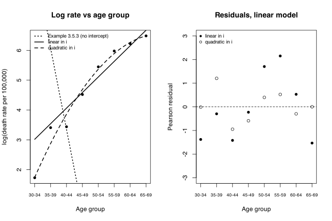
Conclusions. The model of Example 3.5.3 as literally written, with no intercept, is not adequate: it is off by three orders of magnitude and gives a slope of the wrong sign. Its exponential shape is right, and once an intercept is admitted the model \(\log\mu_i = \log n_i + \beta_1 + \beta_2 i\) describes the data reasonably, with the coronary death rate rising by a factor of about \(1.69\) per five-year age band. Even so, the deviance of \(14.69\) on \(6\) df indicates mild lack of fit, and the residual pattern shows the log rate is slightly concave in age; the quadratic model has deviance \(3.09\) on \(5\) df (\(p=0.69\)) and an AIC lower by nearly \(10\), so it is the preferred description. Simple least squares on \(\log(y_i/n_i)\) recovers the same qualitative story but exaggerates the slope and mismatches the observed totals, because it ignores the Poisson mean-variance relationship and the very different amounts of information in the eight groups.
Problem 3.7 — Consider N independent binary random variables Y1 , . . . ,YN with
Consider \(N\) independent binary random variables \(Y_1,\dots,Y_N\) with \[ P(Y_i=1)=\pi_i \quad\text{and}\quad P(Y_i=0)=1-\pi_i. \] The probability function of \(Y_i\), the Bernoulli distribution \(\mathrm{B}(\pi)\), can be written as \[ \pi_i^{y_i}(1-\pi_i)^{1-y_i}, \] where \(y_i = 0\) or \(1\).
a. Show that this probability function belongs to the exponential family of distributions.
b. Show that the natural parameter is \[ \log\left(\frac{\pi_i}{1-\pi_i}\right). \] This function, the logarithm of the odds \(\pi_i/(1-\pi_i)\), is called the logit function.
c. Show that \(\mathrm{E}(Y_i)=\pi_i\).
d. If the link function is \[ g(\pi) = \log\left(\frac{\pi}{1-\pi}\right) = \mathbf{x}^T\boldsymbol\beta, \] show that this is equivalent to modelling the probability \(\pi\) as \[ \pi = \frac{e^{\mathbf{x}^T\boldsymbol\beta}}{1+e^{\mathbf{x}^T\boldsymbol\beta}}. \]
e. In the particular case where \(\mathbf{x}^T\boldsymbol\beta = \beta_1 + \beta_2 x\), this gives \[ \pi = \frac{e^{\beta_1+\beta_2 x}}{1+e^{\beta_1+\beta_2 x}}, \] which is the logistic function. Sketch the graph of \(\pi\) against \(x\) in this case, taking \(\beta_1\) and \(\beta_2\) as constants. How would you interpret this graph if \(x\) is the dose of an insecticide and \(\pi\) is the probability of an insect dying? (difficulty: \(\star\star\))
Part (a). Take logarithms of the probability function and collect terms: \[ f(y_i;\pi_i) = \pi_i^{y_i}(1-\pi_i)^{1-y_i} = \exp\left[ y_i\log\pi_i + (1-y_i)\log(1-\pi_i) \right] = \exp\left[ y_i\log\left(\frac{\pi_i}{1-\pi_i}\right) + \log(1-\pi_i) \right]. \] This is of the form (3.3), \(f(y;\theta)=\exp[a(y)b(\theta)+c(\theta)+d(y)]\), with \[ a(y_i)=y_i, \qquad b(\pi_i)=\log\left(\frac{\pi_i}{1-\pi_i}\right), \qquad c(\pi_i)=\log(1-\pi_i), \qquad d(y_i)=0, \] so the Bernoulli distribution belongs to the exponential family. This is the \(n=1\) case of the Binomial calculation in Section 3.2.3, since \(\binom{1}{y}=1\) and \(n\log(1-\pi)=\log(1-\pi)\).
Part (b). Because \(a(y_i)=y_i\), the distribution is in canonical form, and by the definition in Section 3.2 the natural parameter is \(b(\pi_i)\), that is, \[ b(\pi_i) = \log\left(\frac{\pi_i}{1-\pi_i}\right), \] the logit. This is why the logit is the natural (canonical) link for binary data: with \(g\) equal to the logit, the linear predictor \(\mathbf{x}_i^T\boldsymbol\beta\) is the natural parameter itself.
Part (c). Directly, \(\mathrm{E}(Y_i)=1\cdot\pi_i + 0\cdot(1-\pi_i)=\pi_i\). To use the results of the chapter instead, apply (3.9) with \(a(Y)=Y\): \[ b^{\prime}(\pi_i) = \frac{d}{d\pi_i}\left[\log\pi_i-\log(1-\pi_i)\right] = \frac{1}{\pi_i(1-\pi_i)}, \qquad c^{\prime}(\pi_i) = -\frac{1}{1-\pi_i}, \] so \[ \mathrm{E}(Y_i) = -\frac{c^{\prime}(\pi_i)}{b^{\prime}(\pi_i)} = \frac{1/(1-\pi_i)}{1/[\pi_i(1-\pi_i)]} = \pi_i . \] This is Exercise 3.4(c) with \(n=1\).
Part (d). Exponentiate both sides of \(\log[\pi/(1-\pi)] = \mathbf{x}^T\boldsymbol\beta\): \[ \frac{\pi}{1-\pi} = e^{\mathbf{x}^T\boldsymbol\beta} \implies \pi = (1-\pi)e^{\mathbf{x}^T\boldsymbol\beta} \implies \pi\left(1+e^{\mathbf{x}^T\boldsymbol\beta}\right) = e^{\mathbf{x}^T\boldsymbol\beta}, \] hence \[ \pi = \frac{e^{\mathbf{x}^T\boldsymbol\beta}}{1+e^{\mathbf{x}^T\boldsymbol\beta}} = \frac{1}{1+e^{-\mathbf{x}^T\boldsymbol\beta}} . \] The two statements are equivalent because the logit is a strictly increasing bijection from \((0,1)\) onto \(\mathbb{R}\), with the expression above as its inverse. The practical point is that whatever real value \(\mathbf{x}^T\boldsymbol\beta\) takes, the fitted \(\pi\) automatically lies strictly between \(0\) and \(1\).
Part (e). The graph of \[ \pi(x) = \frac{e^{\beta_1+\beta_2 x}}{1+e^{\beta_1+\beta_2 x}} \] is the sigmoid (“S-shaped”) logistic curve. Its properties, taking \(\beta_2>0\), are as follows. It is strictly increasing, since \[ \frac{d\pi}{dx} = \beta_2\,\pi(1-\pi) > 0 ; \] it has horizontal asymptotes \(\pi \to 0\) as \(x\to-\infty\) and \(\pi \to 1\) as \(x\to+\infty\); it passes through \(\pi = 1/2\) at \(x = -\beta_1/\beta_2\); and it is symmetric about that point, which is also the point of steepest ascent, where the slope equals \(\beta_2/4\). If \(\beta_2<0\) the curve is decreasing, and \(\beta_2=0\) gives a horizontal line at \(\pi = e^{\beta_1}/(1+e^{\beta_1})\). Larger \(|\beta_2|\) makes the transition from \(0\) to \(1\) sharper.
x <- seq(-2, 12, length = 400)
logistic <- function(x, b1, b2) exp(b1 + b2 * x) / (1 + exp(b1 + b2 * x))
par(mfrow = c(1, 2))
plot(x, logistic(x, -5, 1), type = "l", lwd = 2, ylim = c(0, 1),
     xlab = "dose x", ylab = expression(pi),
     main = expression(paste("Logistic curve, ", beta[1] == -5, ", ", beta[2] == 1)))
abline(h = c(0, 0.5, 1), lty = 3); abline(v = 5, lty = 2)
text(5, 0.05, "LD50 = -b1/b2", pos = 4, cex = 0.9)
plot(x, logistic(x, -5, 1), type = "l", lwd = 2, ylim = c(0, 1),
     xlab = "dose x", ylab = expression(pi), main = "Effect of the slope")
lines(x, logistic(x, -2.5, 0.5), lwd = 2, lty = 2)
lines(x, logistic(x, -10, 2), lwd = 2, lty = 3)
legend("topleft", c("b2 = 0.5", "b2 = 1", "b2 = 2"), lty = c(2, 1, 3), lwd = 2, bty = "n")
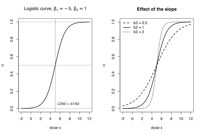
Interpretation as a dose-response curve. If \(x\) is the dose of an insecticide and \(\pi\) the probability that an insect dies, the curve is the classical dose-response relationship.
At very low doses almost no insects die and \(\pi \approx 0\); at very high doses almost all die and \(\pi\approx 1\). Neither extreme is reached exactly, which is realistic: no dose is perfectly safe and no dose is guaranteed lethal.
Over the middle range the response rises steeply, so within a fairly narrow band of doses the kill rate goes from low to high. Outside that band, raising the dose further buys very little extra mortality, which is why the curve flattens.
The dose \(x = -\beta_1/\beta_2\) at which \(\pi = 1/2\) is the median lethal dose, LD50, the standard summary of potency; a more potent insecticide has a smaller LD50. In the left panel, with \(\beta_1=-5\) and \(\beta_2=1\), the LD50 is \(5\) and the maximum slope is \(\beta_2/4 = 0.25\) per unit dose.
The slope \(\beta_2\) has an exact odds interpretation: increasing the dose by one unit adds \(\beta_2\) to the log odds of dying, so it multiplies the odds of death by \(e^{\beta_2}\). This interpretation is constant across the dose range, whereas the effect on the probability is largest near the LD50 and negligible in the tails.
A natural underlying mechanism is a tolerance distribution: suppose insect \(j\) dies if the dose exceeds its individual tolerance \(T_j\), and that \(T_j\) has a logistic distribution across insects. Then \(\pi(x)=P(T_j \le x)\) is exactly the curve above, and the sigmoid shape simply reflects the accumulation of a unimodal spread of tolerances in the population.
Problem 3.8 — Is the extreme value (Gumbel) distribution, with probability density
Is the extreme value (Gumbel) distribution, with probability density function \[ f(y;\theta) = \frac{1}{\phi}\exp\left\{ \frac{(y-\theta)}{\phi} - \exp\left[\frac{(y-\theta)}{\phi}\right] \right\} \] (where \(\phi>0\) is regarded as a nuisance parameter) a member of the exponential family? (difficulty: \(\star\star\))
Yes. Take logarithms and expand the two occurrences of \((y-\theta)/\phi\), remembering that \(\phi\) is treated as known: \[ \log f(y;\theta) = -\log\phi + \frac{y-\theta}{\phi} - \exp\left(\frac{y-\theta}{\phi}\right) = -\log\phi + \frac{y}{\phi} - \frac{\theta}{\phi} - e^{y/\phi}e^{-\theta/\phi}. \] The last term is the only one in which \(y\) and \(\theta\) appear together, and it already factorises as a function of \(y\) times a function of \(\theta\). So \[ f(y;\theta) = \exp\left[ a(y)b(\theta) + c(\theta) + d(y) \right] \] with \[ a(y) = e^{y/\phi}, \qquad b(\theta) = -e^{-\theta/\phi}, \qquad c(\theta) = -\frac{\theta}{\phi} - \log\phi, \qquad d(y) = \frac{y}{\phi}. \] This is form (3.3), so the Gumbel distribution is a member of the exponential family. It is not in canonical form, because \(a(y) = e^{y/\phi} \neq y\). Equivalently, it is \(e^{Y/\phi}\), not \(Y\) itself, that has the canonical exponential-family structure; indeed the calculation above shows \(e^{(Y-\theta)/\phi} \sim \mathrm{Exp}(1)\).
Two conditions were used and are worth stating explicitly. The support of \(f\) is the whole real line and does not depend on \(\theta\), as required for the differentiation-under-the-integral arguments of Section 3.3. And \(\phi\) must genuinely be known: if \(\phi\) were also unknown, \(d(y)=y/\phi\) and \(a(y)=e^{y/\phi}\) would depend on it and the family would be a two-parameter one, outside the one-parameter form (3.3).
Since the distribution is a member of the family, (3.9) and (3.12) apply to \(a(Y)=e^{Y/\phi}\). The derivatives are \[ b^{\prime}(\theta) = \frac{1}{\phi}e^{-\theta/\phi}, \quad b^{\prime\prime}(\theta) = -\frac{1}{\phi^2}e^{-\theta/\phi}, \quad c^{\prime}(\theta) = -\frac{1}{\phi}, \quad c^{\prime\prime}(\theta)=0, \] so from (3.9) \[ \mathrm{E}\left(e^{Y/\phi}\right) = -\frac{c^{\prime}(\theta)}{b^{\prime}(\theta)} = \frac{1/\phi}{e^{-\theta/\phi}/\phi} = e^{\theta/\phi}, \] and from (3.12) \[ \mathrm{var}\left(e^{Y/\phi}\right) = \frac{b^{\prime\prime}c^{\prime} - c^{\prime\prime}b^{\prime}}{[b^{\prime}]^3} = \frac{\left(-\phi^{-2}e^{-\theta/\phi}\right)\left(-\phi^{-1}\right)}{\phi^{-3}e^{-3\theta/\phi}} = e^{2\theta/\phi}. \] Note that these are moments of \(e^{Y/\phi}\), not of \(Y\); the exponential-family machinery gives the mean and variance of \(a(Y)\), and here \(a\) is not the identity. (For the record, \(\mathrm{E}(Y) = \theta - \gamma\phi\) with \(\gamma\) Euler’s constant, which the chapter’s results do not deliver directly.)
Both results are confirmed by simulation, using \(e^{(Y-\theta)/\phi}\sim\mathrm{Exp}(1)\) to generate the variates.
set.seed(7); theta <- 1.3; phi <- 0.7
u <- rexp(2e6)
y <- theta + phi * log(u)
a <- exp(y / phi)
round(c(mean.a = mean(a), theory.mean = exp(theta / phi),
        var.a = var(a),  theory.var = exp(2 * theta / phi)), 4)
mean.a theory.mean       var.a  theory.var
6.4100      6.4054     41.0751     41.0293
Problem 3.9 — Suppose Y1 , . . . ,YN are independent random variables each with the Pareto
Suppose \(Y_1,\dots,Y_N\) are independent random variables each with the Pareto distribution and \[ \mathrm{E}(Y_i) = (\beta_0 + \beta_1 x_i)^2 . \] Is this a generalized linear model? Give reasons for your answer. (difficulty: \(\star\star\))
Check the three components of a generalized linear model listed at the end of Section 3.4.
Component 1: the response distribution. The \(Y_i\) are independent and, by Exercise 3.3(a), each Pareto density \[ f(y;\theta_i) = \theta_i y^{-\theta_i-1}, \qquad y>1, \] belongs to the exponential family, with \(a(y)=\log y\), \(b(\theta_i)=-\theta_i\), \(c(\theta_i)=\log\theta_i\) and \(d(y)=-\log y\). All the \(Y_i\) have the same form of distribution and each depends on a single parameter \(\theta_i\), as required.
There is one caveat, and it should be stated plainly. Dobson’s definition in Section 3.4 asks that each \(Y_i\) have the canonical form \(f(y_i;\theta_i)=\exp[y_ib(\theta_i)+c(\theta_i)+d(y_i)]\), and the Pareto does not: its \(a(y)=\log y\). Taken literally, the model therefore falls outside the definition as written. In practice this is a mild objection, because \(a\) is a fixed known transformation and \(\log Y_i \sim \mathrm{Exp}(\theta_i)\) is canonical, so the same model can be written as a generalized linear model for the transformed response. Most treatments, and the intent of the exercise, accept the Pareto here.
Component 2: the linear component. The systematic part involves \(\beta_0 + \beta_1 x_i\), which is linear in the parameters, with \(\mathbf{x}_i^T = [1\;\;x_i]\) and \(\boldsymbol\beta^T = [\beta_0\;\;\beta_1]\). Note that it is linearity in \(\boldsymbol\beta\) that matters, not linearity in \(x_i\).
Component 3: the link function. We need a monotone differentiable \(g\) with \(g(\mu_i)=\mathbf{x}_i^T\boldsymbol\beta\). Since \(\mu_i = (\beta_0+\beta_1x_i)^2\), take \[ g(\mu) = \sqrt{\mu} = \mu^{1/2}. \] On \(\mu>0\) this is strictly increasing and differentiable, so it is a valid link. (In modern terminology it is the power link with exponent \(1/2\).)
Conclusion. Yes, this is a generalized linear model, with response from the exponential family, linear predictor \(\beta_0+\beta_1x_i\), and link \(g(\mu)=\mu^{1/2}\) – subject to the canonical-form caveat above and to two restrictions on the parameter space that are worth making explicit.
First, \(\sqrt{\cdot}\) inverts \(\mu \mapsto \mu^2\) only on one branch, so \((\beta_0,\beta_1)\) and \((-\beta_0,-\beta_1)\) give identical means. Identifiability requires restricting to \(\beta_0+\beta_1x_i>0\) for all \(i\) in the data.
Second, integrating the Pareto density gives \(\mathrm{E}(Y)=\theta/(\theta-1)\) for \(\theta>1\), which is greater than \(1\) for every admissible \(\theta\) (and the mean does not exist for \(\theta \le 1\)). So the model is coherent only if \((\beta_0+\beta_1x_i)^2>1\), that is \(\beta_0+\beta_1x_i>1\), at every observed \(x_i\). This is a genuine restriction on the parameter space, not a defect of the GLM structure; it is the same kind of restriction that a Binomial model with an identity link would impose.
Problem 3.10 — Let Y1 , . . . ,YN be independent random variables with
Let \(Y_1,\dots,Y_N\) be independent random variables with \[ \mathrm{E}(Y_i) = \mu_i = \beta_0 + \log(\beta_1 + \beta_2 x_i); \qquad Y_i \sim N(\mu,\sigma^2) \] for all \(i=1,\dots,N\). Is this a generalized linear model? Give reasons for your answer. (difficulty: \(\star\))
No, this is not a generalized linear model. It is a nonlinear regression model.
The response distribution is not the problem: the \(Y_i\) are independent and Normal, which is in the exponential family in canonical form (Section 3.2.2). The failure is in the systematic part, which cannot be written as \(g(\mu_i)=\mathbf{x}_i^T\boldsymbol\beta\) for any link \(g\).
To see this, note what such a representation would require. A link function is a fixed known function of \(\mu_i\) alone; it may not involve unknown parameters. Rearranging the model gives \[ \mu_i - \beta_0 = \log(\beta_1+\beta_2x_i), \qquad\text{that is}\qquad e^{\mu_i - \beta_0} = \beta_1 + \beta_2 x_i . \] The right-hand side is linear in \((\beta_1,\beta_2)\), so if \(\beta_0\) were known the model would be a generalized linear model, with link \(g(\mu)=e^{\mu-\beta_0}\) and linear predictor \(\beta_1+\beta_2x_i\). But \(\beta_0\) is unknown and must be estimated, so the candidate link \(g(\mu)=e^{\mu-\beta_0}\) depends on an unknown parameter and is therefore not a link function in the sense of Section 3.4.
Equivalently: in a generalized linear model, all the parameters enter through the single linear combination \(\mathbf{x}_i^T\boldsymbol\beta\). Here \(\beta_0\) enters outside the logarithm while \(\beta_1\) and \(\beta_2\) enter inside it, and there is no transformation \(g\) that puts all three into one linear form. The parameters are not separable in the way the definition requires.
Note also that the three parameters are not all identified without a constraint even in the nonlinear model, because \(\beta_0 + \log(\beta_1+\beta_2x)\) is unchanged if one adds \(\log k\) to \(\beta_0\) and divides both \(\beta_1\) and \(\beta_2\) by \(k\) for any \(k>0\). One would fix this by setting \(\beta_0=0\) or \(\beta_1=1\); with \(\beta_0=0\) the model does become a generalized linear model with link \(g(\mu)=e^{\mu}\).
As written, therefore, the model must be fitted by general nonlinear least squares (for instance R’s nls), not by the iterative weighted least squares of Chapter 4. The model also requires \(\beta_1+\beta_2x_i>0\) at every observation for the logarithm to be defined.
Problem 3.11 — For the Pareto distribution, find the score statistics U and the information
For the Pareto distribution, find the score statistics \(U\) and the information \(\mathfrak{I}=\mathrm{var}(U)\). Verify that \(\mathrm{E}(U)=0\). (difficulty: \(\star\star\))
From Exercise 3.3(a) the Pareto density \(f(y;\theta)=\theta y^{-\theta-1}\), \(y>1\), is in the exponential family with \[ a(y)=\log y, \qquad b(\theta)=-\theta, \qquad c(\theta)=\log\theta, \qquad d(y)=-\log y, \] so the log-likelihood from a single observation is \[ l(\theta;y) = a(y)b(\theta) + c(\theta) + d(y) = -\theta\log y + \log\theta - \log y . \]
The score statistic. Differentiating with respect to \(\theta\), or equivalently using (3.13), \(U = a(Y)b^{\prime}(\theta)+c^{\prime}(\theta)\) with \(b^{\prime}(\theta)=-1\) and \(c^{\prime}(\theta)=1/\theta\), \[ U = \frac{dl}{d\theta} = \frac{1}{\theta} - \log Y . \]
Verification that \(\mathrm{E}(U)=0\). By (3.9), \(\mathrm{E}[a(Y)]=-c^{\prime}(\theta)/b^{\prime}(\theta) = -(1/\theta)/(-1) = 1/\theta\), that is \(\mathrm{E}(\log Y)=1/\theta\). Hence \[ \mathrm{E}(U) = \frac{1}{\theta} - \mathrm{E}(\log Y) = \frac{1}{\theta} - \frac{1}{\theta} = 0, \] which is the general result (3.14). Directly: substituting \(t=\log y\) gives \(\int_1^\infty (\log y)\theta y^{-\theta-1}dy = \int_0^\infty t\,\theta e^{-\theta t}dt = 1/\theta\), since \(\log Y\sim\mathrm{Exp}(\theta)\).
The information. Using \(\mathfrak{I}=\mathrm{var}(U) = [b^{\prime}(\theta)]^2\,\mathrm{var}[a(Y)]\) from Section 3.3, and \(b^{\prime}(\theta)=-1\), \[ \mathfrak{I} = \mathrm{var}(\log Y) = \frac{1}{\theta^2}, \] the variance of an \(\mathrm{Exp}(\theta)\) variate. The same value follows from (3.15) with \(b^{\prime\prime}(\theta)=0\) and \(c^{\prime\prime}(\theta)=-1/\theta^2\): \[ \mathrm{var}(U) = \frac{b^{\prime\prime}(\theta)c^{\prime}(\theta)}{b^{\prime}(\theta)} - c^{\prime\prime}(\theta) = 0 + \frac{1}{\theta^2} = \frac{1}{\theta^2}, \] and from the third form (3.16), \(\mathrm{var}(U)=-\mathrm{E}(U^{\prime})\), since \(U^{\prime} = dU/d\theta = -1/\theta^2\) is non-random here so \(-\mathrm{E}(U^{\prime})=1/\theta^2\).
For a sample. If \(Y_1,\dots,Y_N\) are independent Pareto variables with the same \(\theta\), the log-likelihoods add, so \[ U = \sum_{i=1}^{N}\left(\frac{1}{\theta}-\log Y_i\right) = \frac{N}{\theta} - \sum_{i=1}^{N}\log Y_i, \qquad \mathfrak{I} = \frac{N}{\theta^2}. \] Setting \(U=0\) gives the maximum likelihood estimator \(\hat\theta = N/\sum\log Y_i\), and the asymptotic standard error is \(\mathfrak{I}^{-1/2}=\theta/\sqrt{N}\).
Simulation confirms the two results for a single observation.
set.seed(11); theta <- 2.5
y <- exp(rexp(2e6, rate = theta))
U <- 1 / theta - log(y)
round(c(mean.U = mean(U), theory = 0,
        var.U = var(U), information = 1 / theta^2,
        mean.logY = mean(log(y)), theory.logY = 1 / theta), 5)
 mean.U      theory       var.U information   mean.logY theory.logY
-0.0002      0.0000      0.1603      0.1600      0.4002      0.4000
Problem 3.12 — See some more relationships between distributions in Figure 3.3.
See some more relationships between distributions in Figure 3.3.
Figure 3.3 shows eight boxes joined by arrows, dotted lines indicating an asymptotic relationship and solid lines a transformation. Reading the figure edge by edge: Binomial \(\mathrm{Bin}(n,\pi)\) and Bernoulli \(\mathrm{B}(\pi)\) are joined by a solid double-headed arrow, labelled \(n=1\) in the direction Binomial to Bernoulli and \(X_1+\dots+X_n\) in the direction Bernoulli to Binomial; a dotted arrow runs from Binomial to Poisson \(\mathrm{Po}(\mu)\) labelled \(\mu = n\pi\), \(n\to\infty\); a dotted arrow runs from Negative Binomial \(\mathrm{NBin}(r,\theta)\) to Poisson labelled \(\mu = r(1-\theta)\), \(r\to\infty\); a dotted arrow runs from Poisson to Normal \(N(\mu,\sigma^2)\) labelled \(\sigma^2=\mu\), \(\mu>15\); a dotted arrow runs from Binomial to Normal labelled \(\mu=n\pi\), \(\sigma^2 = n\pi(1-\pi)\), \(n\pi>5\), \(n\pi(1-\pi)>5\); a dotted arrow runs from Gamma \(G(\alpha,\beta)\) to Normal labelled \(\mu=\alpha/\beta\), \(\sigma^2=\alpha/\beta^2\), \(\alpha\to\infty\); a solid arrow runs from Gamma to Exponential \(\mathrm{Exp}(\theta)\) labelled \(\alpha=\theta\), \(\beta=1\); and a solid arrow runs from Standard Uniform \(U(0,1)\) to Exponential labelled \(-\theta\log X\). The Negative Binomial box is joined only to the Poisson box; there is no edge from it to the Normal.
a. Show that the Exponential distribution \(\mathrm{Exp}(\theta)\) is a special case of the Gamma distribution \(G(\alpha,\beta)\).
b. If \(X\) has the Uniform distribution \(U[0,1]\), that is, \(f(x)=1\) for \(0<x<1\), show that \(Y=-\theta\log X\) has the distribution \(\mathrm{Exp}(\theta)\).
c. Use the moment generating functions (or other methods) to show
i. \(\mathrm{Bin}(n,\pi)\to\mathrm{Po}(\lambda)\) as \(n\to\infty\).
ii. \(\mathrm{NBin}(r,\theta)\to\mathrm{Po}(r(1-\theta))\) as \(r\to\infty\).
d. Use the Central Limit Theorem to show
i. \(\mathrm{Po}(\lambda)\to N(\mu,\mu)\) for large \(\mu\).
ii. \(\mathrm{Bin}(n,\pi)\to N(n\pi, n\pi(1-\pi))\) for large \(n\), provided neither \(n\pi\) nor \(n\pi(1-\pi)\) is too small.
iii. \(G(\alpha,\beta)\to N(\alpha/\beta, \alpha/\beta^2)\) for large \(\alpha\). (difficulty: \(\star\star\star\))
Part (a). From Exercise 3.2 the Gamma density with shape \(\alpha\) and rate \(\beta\) is \[ f(y;\alpha,\beta) = \frac{\beta^{\alpha}}{\Gamma(\alpha)}y^{\alpha-1}e^{-y\beta}, \qquad y>0. \] Put \(\alpha=1\) and \(\beta=\theta\). Since \(\Gamma(1)=\int_0^\infty e^{-t}dt = 1\) and \(y^{0}=1\), \[ f(y;1,\theta) = \frac{\theta^{1}}{\Gamma(1)}y^{0}e^{-y\theta} = \theta e^{-y\theta}, \] which is exactly the exponential density of Exercise 3.3(b). So \(\mathrm{Exp}(\theta) = G(1,\theta)\). The moments agree too: Exercise 3.2 gives \(\mathrm{E}(Y)=\alpha/\beta = 1/\theta\) and \(\mathrm{var}(Y)=\alpha/\beta^2 = 1/\theta^2\), the exponential moments. Note that the arrow from Gamma to Exponential in Figure 3.3 is labelled \(\alpha=\theta\), \(\beta=1\), which is the two substitutions interchanged: \(G(\theta,1)\) has density \(y^{\theta-1}e^{-y}/\Gamma(\theta)\), which is exponential only when \(\theta=1\). The correct specialisation is \(\alpha=1\), \(\beta=\theta\), as derived above.
Part (b). Work with the survivor function. Let \(X\sim U[0,1]\) and put \(Y=-\theta\log X\). Since \(0<X<1\) we have \(\log X<0\), so \(Y>0\) as required, and for \(y>0\) \[ P(Y>y) = P(-\theta\log X > y) = P\!\left(\log X < -\frac{y}{\theta}\right) = P\!\left(X < e^{-y/\theta}\right) = e^{-y/\theta}, \] the last step because \(P(X<x)=x\) on \((0,1)\) and \(e^{-y/\theta}\in(0,1)\). Differentiating, the density of \(Y\) is \[ f_Y(y) = -\frac{d}{dy}P(Y>y) = \frac{1}{\theta}e^{-y/\theta}, \qquad y>0, \] so \(Y\) is exponential with mean \(\theta\).
A caution about parametrisation is needed here, and it is the reason to state the result this way. The book’s own exponential density, in Exercise 3.3(b) and Figure 3.3, is \(f(y;\theta)=\theta e^{-y\theta}\), which has mean \(1/\theta\), whereas the density just derived has mean \(\theta\). The two agree only if \(\mathrm{Exp}(\theta)\) is read with \(\theta\) as the scale (the mean). Under the book’s rate parametrisation the correct transformation is \(Y = -\theta^{-1}\log X\), for which the same argument gives \(P(Y>y) = P(X<e^{-\theta y}) = e^{-\theta y}\) and hence density \(\theta e^{-y\theta}\). Equivalently, the statement as printed shows \(-\theta\log X \sim \mathrm{Exp}(1/\theta)\) in the book’s notation. I flag this rather than paper over it; the substance of the result – that \(-\log X\) is a standard exponential variate, which is the basis of inversion sampling – is unaffected.
Part (c)(i): Binomial to Poisson. The moment generating function of \(Y\sim\mathrm{Bin}(n,\pi)\) is \[ M_Y(t) = \mathrm{E}\left(e^{tY}\right) = \sum_{y=0}^n \binom{n}{y}(\pi e^t)^y(1-\pi)^{n-y} = \left(1-\pi+\pi e^t\right)^n . \] Let \(n\to\infty\) with the mean held fixed at \(\lambda = n\pi\), so \(\pi=\lambda/n \to 0\). Then \[ M_Y(t) = \left[1 + \frac{\lambda(e^t-1)}{n}\right]^n \longrightarrow \exp\left[\lambda\left(e^t-1\right)\right], \] using \((1+a/n)^n \to e^a\). The limit is the moment generating function of \(\mathrm{Po}(\lambda)\), since for \(Z\sim\mathrm{Po}(\lambda)\) \[ M_Z(t) = \sum_{z=0}^\infty e^{tz}\frac{\lambda^z e^{-\lambda}}{z!} = e^{-\lambda}\sum_{z=0}^\infty \frac{(\lambda e^t)^z}{z!} = \exp\left[\lambda(e^t-1)\right]. \] By the continuity theorem for moment generating functions, \(\mathrm{Bin}(n,\lambda/n)\to\mathrm{Po}(\lambda)\). This is the “law of small numbers”: many trials, each very unlikely to succeed, with a stable expected number of successes.
Part (c)(ii): Negative Binomial to Poisson. With \(Y\sim\mathrm{NBin}(r,\theta)\) counting failures before the \(r\)th success, as in Exercise 3.3(c), \[ M_Y(t) = \sum_{y=0}^\infty e^{ty}\binom{y+r-1}{r-1}\theta^r(1-\theta)^y = \theta^r\sum_{y=0}^\infty\binom{y+r-1}{r-1}\left[(1-\theta)e^t\right]^y = \left[\frac{\theta}{1-(1-\theta)e^t}\right]^r, \] valid for \((1-\theta)e^t<1\), using the negative binomial series \(\sum_y \binom{y+r-1}{r-1}u^y = (1-u)^{-r}\). Now let \(r\to\infty\) with \(\lambda = r(1-\theta)\) fixed, so \(1-\theta = \lambda/r \to 0\). Taking logarithms, \[ \log M_Y(t) = r\left[\log\left(1-\frac{\lambda}{r}\right) - \log\left(1-\frac{\lambda e^t}{r}\right)\right] = r\left[\left(-\frac{\lambda}{r}+O(r^{-2})\right) - \left(-\frac{\lambda e^t}{r}+O(r^{-2})\right)\right], \] which tends to \(\lambda(e^t-1)\). Hence \(M_Y(t)\to\exp[\lambda(e^t-1)]\) and \(\mathrm{NBin}(r,\theta)\to\mathrm{Po}(r(1-\theta))\). This is consistent with the moments found in Exercise 3.5: as \(\theta\to1\) the ratio \(\mathrm{var}(Y)/\mathrm{E}(Y) = 1/\theta \to 1\), the Poisson value, so the overdispersion vanishes in the limit.
Both limits are checked numerically by the largest absolute discrepancy between the probability functions, with \(\lambda=3\) throughout.
lam <- 3
k <- 0:30
bin.err <- sapply(c(10, 50, 200, 5000),
                  function(n) max(abs(dbinom(k, n, lam / n) - dpois(k, lam))))
nb.err  <- sapply(c(5, 25, 100, 2000),
                  function(r) max(abs(dnbinom(k, size = r, prob = 1 - lam / r) - dpois(k, lam))))
out <- rbind(Bin.to.Po = bin.err, NBin.to.Po = nb.err)
colnames(out) <- c("n or r = 10/5", "50/25", "200/100", "5000/2000")
signif(out, 3)
           n or r = 10/5   50/25 200/100 5000/2000
Bin.to.Po         0.0428 0.00702 0.00170  6.72e-05
NBin.to.Po        0.1690 0.03250 0.00792  3.92e-04
Part (d): the Normal limits. The Central Limit Theorem states that if \(X_1,\dots,X_n\) are independent and identically distributed with mean \(m\) and finite variance \(v\), then \(\sum X_j\) is asymptotically \(N(nm, nv)\). In each case below the trick is to write the distribution as a sum of independent identically distributed pieces, which is possible because all three families are closed under convolution (reproductive).
(i) Poisson. If \(\mu\) is a positive integer, \(Y\sim\mathrm{Po}(\mu)\) has the same distribution as \(X_1+\dots+X_\mu\) where the \(X_j\) are independent \(\mathrm{Po}(1)\) variables, each with mean \(1\) and variance \(1\) (Exercise 3.4(a)). By the Central Limit Theorem \(Y\) is asymptotically \(N(\mu,\mu)\) as \(\mu\to\infty\). For non-integer \(\mu\) the same conclusion follows by writing \(Y\) as a sum of \(n\) independent \(\mathrm{Po}(\mu/n)\) variables and letting \(n\to\infty\) suitably, or by a direct characteristic-function argument; the essential point is that \(\mu\) large means many independent contributions. The rule of thumb printed in Figure 3.3 is \(\mu>15\).
(ii) Binomial. Here the decomposition is exact and immediate: \(Y\sim\mathrm{Bin}(n,\pi)\) is the sum \(X_1+\dots+X_n\) of independent Bernoulli variables with \(\mathrm{E}(X_j)=\pi\) and \(\mathrm{var}(X_j)=\pi(1-\pi)\) (Exercise 3.7). The Central Limit Theorem gives \(Y\) asymptotically \(N(n\pi, n\pi(1-\pi))\). The proviso matters: the Bernoulli summands are skew unless \(\pi=1/2\), and the standardised skewness of \(Y\) is \[ \frac{1-2\pi}{\sqrt{n\pi(1-\pi)}} , \] which is only small when \(n\pi(1-\pi)\) is large. If \(\pi\) is very small the boundary at \(0\) truncates the would-be Normal shape and the Poisson limit of part (c)(i) is the appropriate approximation instead. Hence the conditions \(n\pi>5\) and \(n\pi(1-\pi)>5\) in Figure 3.3.
(iii) Gamma. If \(\alpha\) is a positive integer, \(Y\sim G(\alpha,\beta)\) is the sum of \(\alpha\) independent \(\mathrm{Exp}(\beta) = G(1,\beta)\) variables by part (a), each with mean \(1/\beta\) and variance \(1/\beta^2\). The Central Limit Theorem then gives \(Y\) asymptotically \(N(\alpha/\beta, \alpha/\beta^2)\) as \(\alpha\to\infty\), matching the moments found in Exercise 3.2. For general real \(\alpha>0\), write \(\alpha = n(\alpha/n)\) and use \(G(\alpha,\beta) = \sum_{j=1}^n G(\alpha/n,\beta)\) independently, which is legitimate because the Gamma family is closed under convolution in the shape parameter.
In all three cases the underlying reason is the same: the coefficient of variation is \(O(\alpha^{-1/2})\), so as the shape or count parameter grows, the distribution concentrates and its standardised form flattens out to the Normal. The approximations are checked by the largest absolute difference between the exact and Normal cumulative distribution functions, with a continuity correction in the two discrete cases.
cc <- function(q, m, v) pnorm(q + 0.5, m, sqrt(v))
po <- sapply(c(5, 20, 100), function(mu) { k <- 0:ceiling(mu + 10 * sqrt(mu))
                 max(abs(ppois(k, mu) - cc(k, mu, mu))) })
bi <- sapply(c(10, 50, 500), function(n) { k <- 0:n
                 max(abs(pbinom(k, n, 0.3) - cc(k, n * 0.3, n * 0.3 * 0.7))) })
ga <- sapply(c(2, 10, 100), function(a) { q <- seq(0, a + 10 * sqrt(a), length = 2000)
                 max(abs(pgamma(q, shape = a, rate = 1) - pnorm(q, a, sqrt(a)))) })
out <- rbind(Po.mu = po, Bin.n = bi, Gamma.alpha = ga)
colnames(out) <- c("small", "medium", "large")
round(out, 4)
             small medium  large
Po.mu       0.0290 0.0148 0.0066
Bin.n       0.0177 0.0081 0.0026
Gamma.alpha 0.0945 0.0421 0.0133
The parameter values are \(\mu = 5, 20, 100\) for the Poisson, \(n = 10, 50, 500\) with \(\pi=0.3\) for the Binomial, and \(\alpha = 2, 10, 100\) with \(\beta=1\) for the Gamma. In every row the error falls roughly as the square root of the parameter, the rate the Berry-Esseen bound predicts, and at \(\mu=20\), \(n=50\) and \(\alpha=100\) the maximum error is at or below about \(1.5\%\), which is why the rules of thumb quoted in Figure 3.3 are set where they are.
The practical relevance for this chapter is that these limits are what license the large-sample approximations used throughout the book: the Normal approximations to the sampling distributions of estimators in Chapter 4, the \(\chi^2\) approximations to deviances in Chapter 5, and the interchangeable use of Poisson and Binomial models for rare events.
Estimation
Problem 4.1 — The data in Table 4.5 show the numbers of cases of AIDS in Australia
The data in Table 4.5 show the numbers of cases of AIDS in Australia by date of diagnosis for successive 3-month periods from 1984 to 1988. (Data from National Centre for HIV Epidemiology and Clinical Research, 1994.)
Table 4.5 gives, for each year 1984–1988, the number of cases in quarters 1, 2, 3 and 4 respectively: 1984: 1, 6, 16, 23; 1985: 27, 39, 31, 30; 1986: 43, 51, 63, 70; 1987: 88, 97, 91, 104; 1988: 110, 113, 149, 159. Reading across rows gives the \(N = 20\) successive quarterly counts \(y_1, \ldots, y_{20}\).
In this early phase of the epidemic, the numbers of cases seemed to be increasing exponentially.
- (a)
- Plot the number of cases \(y_i\) against time period \(i\) (\(i = 1, \ldots, 20\)).
- (b)
- A possible model is the Poisson distribution with parameter \(\lambda_i = i^{\theta}\), or equivalently \[ \log \lambda_i = \theta \log i. \] Plot \(\log y_i\) against \(\log i\) to examine this model.
- (c)
- Fit a generalized linear model to these data using the Poisson distribution, the log-link function and the equation \[ g(\lambda_i) = \log \lambda_i = \beta_1 + \beta_2 x_i, \] where \(x_i = \log i\). Firstly, do this from first principles, working out expressions for the weight matrix \(\mathbf{W}\) and other terms needed for the iterative equation \[ \mathbf{X}^T \mathbf{W} \mathbf{X} \mathbf{b}^{(m)} = \mathbf{X}^T \mathbf{W} \mathbf{z} \] and using software which can perform matrix operations to carry out the calculations.
- (d)
- Fit the model described in (c) using statistical software which can perform Poisson regression. Compare the results with those obtained in (c).
(difficulty: \(\star\star\))
Part (a) — the raw series.
library(dobson)
data(aids)
y <- aids$cases
i <- seq_along(y)
plot(i, y, pch = 19, xlab = "time period i (quarters from 1984)",
     ylab = expression(y[i]~"(cases of AIDS)"),
     main = "AIDS cases in Australia by quarter, 1984-1988")
lines(i, y, lty = 3)
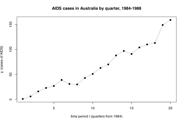
The counts rise monotonically apart from small wobbles at \(i = 7,8\) (1985 quarters 3–4) and \(i = 15\) (1987 quarter 3). The growth is clearly not linear: the increment per quarter is about 5 cases early on and about 15 cases at the end. The scatter about any smooth trend also widens with the level of the series, which is exactly the mean–variance behaviour \(\operatorname{var}(Y_i) = \operatorname{E}(Y_i)\) that motivates a Poisson model here.
Part (b) — the log–log plot.
Under \(\lambda_i = i^{\theta}\) we have \(\log \lambda_i = \theta \log i\), so a plot of \(\log y_i\) against \(\log i\) should be roughly a straight line through the origin with slope \(\theta\).
plot(log(i), log(y), pch = 19, xlab = expression(log~i),
     ylab = expression(log~y[i]), main = "log-log plot of AIDS counts")
abline(lm(log(y) ~ log(i)), lty = 2)
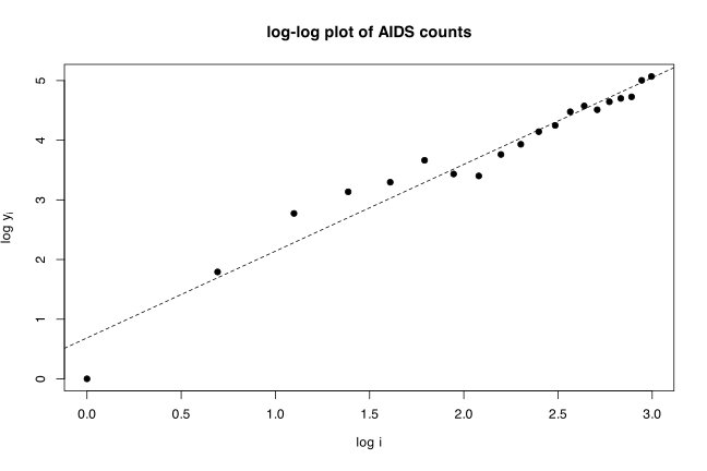
The points lie close to a straight line, so the power-law mean \(\lambda_i = i^{\theta}\) is a reasonable description; an ordinary least-squares line through the log–log points has slope \(1.454\) and intercept \(0.686\). The intercept is not zero, which is why part (c) generalises the model to \(\log \lambda_i = \beta_1 + \beta_2 x_i\) with \(x_i = \log i\): the one-parameter model \(\lambda_i = i^{\theta}\) is the special case \(\beta_1 = 0\). Note also that the first observation (\(i = 1\), \(y_1 = 1\)) sits at the origin of this plot and is the point furthest below the line; the log transformation exaggerates its influence, which is another reason to fit the Poisson GLM properly rather than to regress \(\log y_i\) on \(\log i\).
Part (c) — iterative weighted least squares from first principles.
The model is \(Y_i \sim \operatorname{Po}(\lambda_i)\) independently, with \(\eta_i = \log \lambda_i = \beta_1 + \beta_2 x_i = \mathbf{x}_i^T \boldsymbol\beta\) and \(x_i = \log i\). Write \(\mu_i = \lambda_i\) for the mean. Then
\[ \mu_i = e^{\eta_i}, \qquad \frac{\partial \mu_i}{\partial \eta_i} = e^{\eta_i} = \mu_i, \qquad \operatorname{var}(Y_i) = \mu_i . \]
From equation (4.23) the diagonal weights are
\[ w_{ii} = \frac{1}{\operatorname{var}(Y_i)} \left( \frac{\partial \mu_i}{\partial \eta_i} \right)^{2} = \frac{\mu_i^{2}}{\mu_i} = \mu_i , \]
so \(\mathbf{W} = \operatorname{diag}(\mu_1, \ldots, \mu_N)\) — a consequence of the log link being the canonical link for the Poisson distribution, for which the weights reduce to the variance function itself. From equation (4.24) the working response is
\[ z_i = \sum_{k=1}^{p} x_{ik} b_k^{(m-1)} + (y_i - \mu_i) \frac{\partial \eta_i}{\partial \mu_i} = \eta_i + \frac{y_i - \mu_i}{\mu_i} , \]
with \(\eta_i\) and \(\mu_i\) evaluated at \(\mathbf{b}^{(m-1)}\). The design matrix is \(\mathbf{X}\) with rows \((1, \log i)\), and the information matrix is \(\mathfrak{I} = \mathbf{X}^T \mathbf{W} \mathbf{X}\) with entries
\[ \mathfrak{I} = \begin{bmatrix} \sum_i \mu_i & \sum_i \mu_i x_i \\ \sum_i \mu_i x_i & \sum_i \mu_i x_i^{2} \end{bmatrix}, \qquad \mathbf{X}^T \mathbf{W} \mathbf{z} = \begin{bmatrix} \sum_i \mu_i \eta_i + (y_i - \mu_i) \\ \sum_i x_i \left[ \mu_i \eta_i + (y_i - \mu_i) \right] \end{bmatrix} . \]
Solving \(\mathbf{X}^T \mathbf{W} \mathbf{X} \mathbf{b}^{(m)} = \mathbf{X}^T \mathbf{W} \mathbf{z}\) repeatedly, starting from the log–log fit of part (b):
x <- log(i)
X <- cbind(1, x)
b <- c(0.5, 1.5)                          # rough start suggested by the log-log plot
for (m in 1:6) {
  eta <- X %*% b
  mu  <- exp(eta)                         # inverse log link
  W   <- diag(as.vector(mu))              # w_ii = (dmu/deta)^2 / var(Y) = mu_i
  z   <- eta + (y - mu)/mu                # z_i = eta_i + (y_i - mu_i) deta/dmu
  b   <- solve(t(X) %*% W %*% X, t(X) %*% W %*% z)
  cat(sprintf("m = %d   b1 = %.6f   b2 = %.6f\n", m, b[1], b[2]))
}
m = 1   b1 = 1.054285   b2 = 1.305697
m = 2   b1 = 0.996735   b2 = 1.326344
m = 3   b1 = 0.995998   b2 = 1.326610
m = 4   b1 = 0.995998   b2 = 1.326610
m = 5   b1 = 0.995998   b2 = 1.326610
m = 6   b1 = 0.995998   b2 = 1.326610
Convergence is essentially complete after three iterations, as in Table 4.4 for the worked example of Section 4.4. The maximum likelihood estimates are \(\widehat\beta_1 = 0.99600\) and \(\widehat\beta_2 = 1.32661\). The inverse of the information matrix at the estimates gives the standard errors, by equation (4.12) generalised to the vector case:
I <- t(X) %*% diag(as.vector(exp(X %*% b))) %*% X
I
solve(I)
sqrt(diag(solve(I)))
                  x
  1311.000 3396.379
x 3396.379 9038.301
                        x
   0.02880067 -0.01082261
x -0.01082261  0.00417752
                    x
0.16970761 0.06463374
Part (d) — the same model via Poisson regression software.
aids$i <- seq_len(nrow(aids))
res.p <- glm(cases ~ log(i), family = poisson(link = "log"), data = aids)
summary(res.p)
Call:
glm(formula = cases ~ log(i), family = poisson(link = "log"),
    data = aids)

Coefficients:
            Estimate Std. Error z value Pr(>|z|)
(Intercept)  0.99600    0.16971   5.869 4.39e-09 ***
log(i)       1.32661    0.06463  20.525  < 2e-16 ***
---
Signif. codes:  0 ‘***’ 0.001 ‘**’ 0.01 ‘*’ 0.05 ‘.’ 0.1 ‘ ’ 1

(Dispersion parameter for poisson family taken to be 1)

    Null deviance: 677.264  on 19  degrees of freedom
Residual deviance:  21.755  on 18  degrees of freedom
AIC: 138.05

Number of Fisher Scoring iterations: 4
(Note the explicit poisson(link = "log"): after library(dobson) the bare name poisson refers to the package’s data set of Table 4.3, not to the family function.)
The estimates and standard errors agree with part (c) to every printed digit — \(b_1 = 0.99600\,(0.16971)\), \(b_2 = 1.32661\,(0.06463)\) — which is what we expect, since glm uses precisely the algorithm of equation (4.25) and, for the canonical link, Fisher scoring and Newton–Raphson coincide.
On interpretation and adequacy: the fitted mean is \(\widehat\lambda_i = e^{0.996} i^{1.327} = 2.71\, i^{1.327}\): the quarterly incidence grows as a power of time with exponent about \(1.33\), not exponentially in \(i\). An approximate 95% confidence interval for \(\beta_2\) is \(1.3266 \pm 1.96 \times 0.0646 = (1.200, 1.453)\), which excludes \(1\), so the growth is faster than linear in \(i\) but far short of the doubling behaviour that “increasing exponentially” would suggest. The one-parameter model of part (b), \(\beta_1 = 0\), is decisively rejected (\(z = 5.87\)).
The residual deviance is \(21.755\) on \(18\) degrees of freedom, \(p = 0.243\) against \(\chi^2(18)\), so there is no evidence of lack of fit or of overdispersion. Compare the alternative log-linear-in-time model \(\log \lambda_i = \beta_1 + \beta_2 i\), which is the literal “exponential growth” hypothesis:
m.pow <- glm(cases ~ log(i), family = poisson(link = "log"), data = aids)
m.exp <- glm(cases ~ i,      family = poisson(link = "log"), data = aids)
c(power.dev = deviance(m.pow), power.AIC = AIC(m.pow),
  exp.dev = deviance(m.exp), exp.AIC = AIC(m.exp))
power.dev power.AIC   exp.dev   exp.AIC
 21.75511 138.05303  53.02000 169.31792
The power-law model is far better (deviance \(21.8\) versus \(53.0\) on the same \(18\) degrees of freedom; the exponential-growth model has \(p = 2.6 \times 10^{-5}\) for lack of fit, and its AIC is \(31\) units worse). Substantively, the epidemic was already decelerating on the log scale by 1988.
par(mfrow = c(1, 2))
plot(aids$i, aids$cases, pch = 19, xlab = "quarter i", ylab = "cases",
     main = "Fitted Poisson power-law mean")
lines(aids$i, fitted(m.pow), lwd = 2)
plot(aids$i, residuals(m.pow, type = "deviance"), pch = 19,
     xlab = "quarter i", ylab = "deviance residual", main = "Deviance residuals")
abline(h = 0, lty = 2)
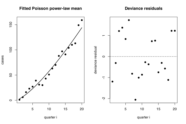
The fitted curve tracks the counts closely and the deviance residuals show no trend and no funnelling; they run from \(-2.06\) (at \(i = 8\), the 1985 fourth quarter, where the series briefly flattens) to \(1.73\), so a single residual just crosses \(-2\) and nothing else is close to the boundary. The model is adequate.
Problem 4.2 — The data in Table 4.6 are times to death, yi , in weeks from diagnosis and
The data in Table 4.6 are times to death, \(y_i\), in weeks from diagnosis and \(\log_{10}\) (initial white blood cell count), \(x_i\), for seventeen patients suffering from leukemia. (This is Example U from Cox and Snell, 1981.)
Table 4.6 lists the seventeen pairs \((y_i, x_i)\) as: \((65, 3.36)\), \((156, 2.88)\), \((100, 3.63)\), \((134, 3.41)\), \((16, 3.78)\), \((108, 4.02)\), \((121, 4.00)\), \((4, 4.23)\), \((39, 3.73)\), \((143, 3.85)\), \((56, 3.97)\), \((26, 4.51)\), \((22, 4.54)\), \((1, 5.00)\), \((1, 5.00)\), \((5, 4.72)\), \((65, 5.00)\).
- (a)
- Plot \(y_i\) against \(x_i\). Do the data show any trend?
- (b)
- A possible specification for \(\operatorname{E}(Y)\) is \[ \operatorname{E}(Y_i) = \exp(\beta_1 + \beta_2 x_i), \] which will ensure that \(\operatorname{E}(Y)\) is non-negative for all values of the parameters and all values of \(x\). Which link function is appropriate in this case?
- (c)
- The Exponential distribution is often used to describe survival times. The probability distribution is \(f(y; \theta) = \theta e^{-y \theta}\). This is a special case of the Gamma distribution with shape parameter \(\phi = 1\) (see Exercise 3.12(a)). Show that \(\operatorname{E}(Y) = 1/\theta\) and \(\operatorname{var}(Y) = 1/\theta^{2}\).
- (d)
- Fit a model with the equation for \(\operatorname{E}(Y_i)\) given in (b) and the Exponential distribution using appropriate statistical software.
- (e)
- For the model fitted in (d), compare the observed values \(y_i\) and fitted values \(\widehat y_i = \exp(\widehat\beta_1 + \widehat\beta_2 x_i)\), and use the standardized residuals \(r_i = (y_i - \widehat y_i) / \widehat y_i\) to investigate the adequacy of the model. (Note: \(\widehat y_i\) is used as the denominator of \(r_i\) because it is an estimate of the standard deviation of \(Y_i\) — see (c) above.)
(difficulty: \(\star\star\))
Each \(y_i\) is time to death for a particular leukemia patient, in weeks from diagnosis; the \(x_i\) are \(\log_{10}\) initial white blood cell counts.
Part (a) — scatter plot.
library(dobson)
data(leukemia)
x <- leukemia$wbc
y <- leukemia$time
plot(x, y, pch = 19, xlab = "x (log10 initial white blood cell count)",
     ylab = "y (survival time, weeks)",
     main = "Survival time against log10 WBC, 17 leukemia patients")
lines(lowess(x, y), lty = 2)
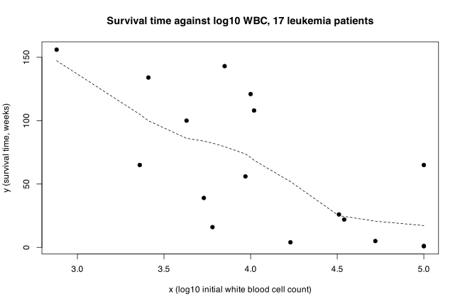
length(x) # 17 patients
[1] 17
The data show a clear negative trend: as the initial white cell count rises, survival time falls. Two further features matter for the modelling. First, the spread of \(y\) shrinks with \(x\) — at \(x \approx 3\) survival ranges over roughly \(16\) to \(156\) weeks, while at \(x = 5\) the three patients survived \(1\), \(1\) and \(65\) weeks. Variability therefore scales with the level, ruling out constant-variance least squares. Second, the decline looks curved rather than straight, consistent with a multiplicative (exponential) rather than additive effect of \(x\).
Part (b) — link function.
\[ \operatorname{E}(Y_i) = \exp(\beta_1 + \beta_2 x_i) \iff \log \operatorname{E}(Y_i) = \beta_1 + \beta_2 x_i , \]
so the appropriate link is the log link, \(g(\mu) = \log \mu\), in the notation \(g(\mu_i) = \mathbf{x}_i^T \boldsymbol\beta\) of equation (4.16).
This is the natural choice here for three reasons. Survival time is strictly positive, and the exponential mean function guarantees \(\operatorname{E}(Y) > 0\) for all \(\beta\) and all \(x\), unlike an identity link which can predict negative survival times. The variance scales with the mean (survival times are right-skewed), so a constant-variance assumption is inappropriate; the Gamma/exponential family with a log link handles this directly. Finally the log link linearises a multiplicative relationship — a unit increase in \(x_i\) multiplies \(\operatorname{E}(Y)\) by \(e^{\beta_2}\) — which is the more natural form for this biological relationship. The negative trend in (a) implies \(\beta_2 < 0\).
Part (c) — moments of the exponential distribution.
\[ f(y; \theta) = \theta e^{-y\theta}, \qquad y > 0, \]
which is the Gamma density with shape parameter \(\phi = 1\). For the mean, integrate by parts with \(u = y\) and \(\mathrm{d}v = \theta e^{-y\theta}\,\mathrm{d}y\):
\[ \operatorname{E}(Y) = \int_0^{\infty} y \cdot \theta e^{-y\theta}\,\mathrm{d}y = \left[ -y e^{-y\theta} \right]_0^{\infty} + \int_0^{\infty} e^{-y\theta}\,\mathrm{d}y = 0 + \left[ -\frac{1}{\theta} e^{-y\theta} \right]_0^{\infty} = \frac{1}{\theta}. \]
For the second moment, two applications of integration by parts (or the Gamma integral \(\int_0^{\infty} y^n e^{-y\theta}\,\mathrm{d}y = n! / \theta^{n+1}\)) give
\[ \operatorname{E}(Y^{2}) = \theta \cdot \frac{2!}{\theta^{3}} = \frac{2}{\theta^{2}}, \]
whence
\[ \operatorname{var}(Y) = \operatorname{E}(Y^{2}) - \left[ \operatorname{E}(Y) \right]^{2} = \frac{2}{\theta^{2}} - \frac{1}{\theta^{2}} = \frac{1}{\theta^{2}} . \]
Note that \(\operatorname{var}(Y) = \left[ \operatorname{E}(Y) \right]^{2}\), confirming the Gamma variance structure \(\operatorname{var}(Y) = \phi \left[ \operatorname{E}(Y) \right]^{2}\) with \(\phi = 1\). This is the fact that part (e) exploits: the standard deviation of \(Y_i\) equals its mean.
Part (d) — fitting the model.
fit <- glm(y ~ x, family = Gamma(link = "log"), data = data.frame(x, y))
summary(fit)
Call:
glm(formula = y ~ x, family = Gamma(link = "log"), data = data.frame(x,
    y))

Coefficients:
            Estimate Std. Error t value Pr(>|t|)
(Intercept)   8.4775     1.6034   5.287 9.13e-05 ***
x            -1.1093     0.3872  -2.865   0.0118 *
---
Signif. codes:  0 ‘***’ 0.001 ‘**’ 0.01 ‘*’ 0.05 ‘.’ 0.1 ‘ ’ 1

(Dispersion parameter for Gamma family taken to be 0.9388638)

    Null deviance: 26.282  on 16  degrees of freedom
Residual deviance: 19.457  on 15  degrees of freedom
AIC: 173.97

Number of Fisher Scoring iterations: 8
We use Gamma(link = "log") because the exponential distribution is the special case of the Gamma family with \(\phi = 1\), and the log link is the mean function \(\operatorname{E}(Y_i) = \exp(\beta_1 + \beta_2 x_i)\) of part (b). The maximum likelihood estimates of \(\boldsymbol\beta\) do not depend on \(\phi\) at all — \(\phi\) cancels out of the score equations (4.18), since it enters \(\operatorname{var}(Y_i)\) as a constant multiplier — so these are exactly the exponential-model estimates. Only the standard errors are affected, and by default glm estimates \(\phi\) from the data rather than fixing it at \(1\). Imposing \(\phi = 1\), as the exponential assumption requires:
summary(fit, dispersion = 1)$coefficients
             Estimate Std. Error   z value     Pr(>|z|)
(Intercept)  8.477494  1.6548077  5.122948 3.007955e-07
x           -1.109297  0.3996545 -2.775640 5.509317e-03
The standard errors change only slightly (from \(1.603\) to \(1.655\) and from \(0.387\) to \(0.400\)), because \(\widehat\phi = 0.939\) is already close to \(1\).
On interpretation: \(\widehat\beta_2 = -1.109\), confirming the negative trend of part (a). On the original scale, an increase of one unit in \(\log_{10}\) (white cell count) — that is, a tenfold increase in the count — multiplies expected survival by \(e^{-1.109} = 0.33\), so it cuts expected survival to about a third. A 95% confidence interval for \(\beta_2\) using the exponential (\(\phi = 1\)) standard error is \(-1.109 \pm 1.96 \times 0.400 = (-1.893, -0.326)\), giving a multiplicative factor between \(0.15\) and \(0.72\); the effect is clearly established in direction, though its size is imprecisely determined with only 17 patients. The fitted mean survival runs from \(\widehat y = 197\) weeks at \(x = 2.88\) down to \(\widehat y = 19\) weeks at \(x = 5.00\).
Part (e) — standardized residuals.
For the exponential (Gamma with \(\phi = 1\)) model, part (c) gives \(\operatorname{var}(Y_i) = \left[ \operatorname{E}(Y_i) \right]^{2}\), so the standard deviation equals the mean: \(\operatorname{sd}(Y_i) = \operatorname{E}(Y_i)\). Dividing the raw residual by \(\widehat y_i\) therefore divides by the estimated standard deviation, which is what makes
\[ r_i = \frac{y_i - \widehat y_i}{\widehat y_i}, \qquad \widehat y_i = \exp(\widehat\beta_1 + \widehat\beta_2 x_i) \]
a genuinely standardized residual rather than an ad hoc scaling. These are exactly the Pearson residuals for the Gamma family.
b1 <- coef(fit)[1]
b2 <- coef(fit)[2]

yhat <- exp(b1 + b2*x)     # equivalently fitted(fit)
r    <- (y - yhat) / yhat  # equivalently residuals(fit, type = "pearson")

par(mfrow = c(1, 2))
plot(yhat, r, xlab = expression(hat(y)[i]), ylab = expression(r[i]),
     main = "Residuals vs fitted", pch = 19); abline(h = 0, lty = 2)
plot(x, r, xlab = "x (log10 WBC)", ylab = expression(r[i]),
     main = "Residuals vs x", pch = 19); abline(h = 0, lty = 2)
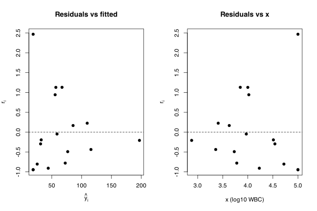
data.frame(x, y, yhat = round(yhat, 2), r = round(r, 3))
      x   y   yhat      r
1  3.36  65 115.61 -0.438
2  2.88 156 196.90 -0.208
3  3.63 100  85.69  0.167
4  3.41 134 109.38  0.225
5  3.78  16  72.56 -0.779
6  4.02 108  55.60  0.943
7  4.00 121  56.84  1.129
8  4.23   4  44.04 -0.909
9  3.73  39  76.69 -0.491
10 3.85 143  67.13  1.130
11 3.97  56  58.77 -0.047
12 4.51  26  32.28 -0.195
13 4.54  22  31.23 -0.295
14 5.00   1  18.75 -0.947
15 5.00   1  18.75 -0.947
16 4.72   5  25.57 -0.804
17 5.00  65  18.75  2.467
On the adequacy of the model:
Centre and spread. The residuals are centred near zero and have \(\operatorname{sd}(r_i) = 0.938\). Because the model implies \(\operatorname{sd}(Y_i) = \operatorname{E}(Y_i)\), a typical residual should have magnitude about \(1\), and indeed all but one observation fall in roughly \((-0.95, 1.13)\). This is consistent with the exponential assumption: observations routinely sit a full standard deviation from their fitted mean, which for this distribution is expected rather than alarming. Note also that \(r_i\) is bounded below by \(-1\) (since \(y_i > 0\)) and unbounded above, so the visible right skew of the residuals is a property of the distribution, not evidence against it.
Link to the dispersion parameter. Since these are Pearson residuals, \(\widehat\phi = \frac{1}{n - p}\sum r_i^{2} = \frac{1}{15}\sum r_i^{2} = 0.939\), matching the dispersion reported in part (d). Its closeness to \(1\) supports the choice \(\phi = 1\), that is, the exponential rather than a general Gamma.
Deviance. Under the exponential assumption \(\phi = 1\) the residual deviance printed in part (d) is already the scaled deviance, \(D = 19.457\) on \(15\) degrees of freedom. Referred to \(\chi^2(15)\) this gives \(p = 0.194\), so there is no evidence of lack of fit. (Had \(\phi\) been estimated, the deviance would need dividing by \(\widehat\phi\) before this comparison; here \(\widehat\phi \approx 1\) so it makes almost no difference.)
Structure. Plotting \(r_i\) against \(\widehat y_i\) and against \(x_i\) shows no obvious funnelling and no systematic curvature, so the log link and the mean function \(\operatorname{E}(Y_i) = \exp(\beta_1 + \beta_2 x_i)\) appear appropriate. Modelling on the log scale has removed the mean–variance dependence visible in the raw data of part (a).
One outlier. The last observation (\(x = 5.00\), \(y = 65\)) gives \(r_{17} = 2.47\), well outside the others. Three patients share the highest count \(x = 5.00\); two survived \(1\) week while the third survived \(65\), so the model, which fits \(\widehat y = 18.75\) for all three, cannot accommodate that spread. Under the exponential distribution \(\Pr(Y > 3.47\,\mu) = e^{-3.47} = 0.031\), so a residual this large among 17 observations is unusual but not extraordinary. It is a genuinely surprising survival rather than a model failure, though it does inflate the residual sum of squares.
Overall the exponential model is adequate: the standardized residuals are unstructured, their spread is close to \(1\), and the estimated dispersion is close to the assumed \(\phi = 1\). The single high-leukocyte survivor is the only notable departure.
Problem 4.3 — Let Y1 , . . . ,YN be a random sample from the Normal distribution Yi \(\sim\)
Let \(Y_1, \ldots, Y_N\) be a random sample from the Normal distribution \(Y_i \sim N(\log \beta, \sigma^{2})\) where \(\sigma^{2}\) is known. Find the maximum likelihood estimator of \(\beta\) from first principles. Also verify Equations (4.18) and (4.25) in this case. (difficulty: \(\star\star\))
First, the maximum likelihood estimator from first principles.
The joint density of the sample is a product of Normal densities with common mean \(\log\beta\) and known variance \(\sigma^{2}\), so the log-likelihood is
\[ l(\beta; y_1, \ldots, y_N) = -\frac{1}{2\sigma^{2}} \sum_{i=1}^{N} (y_i - \log \beta)^{2} - N \log \left( \sigma \sqrt{2\pi} \right) . \]
Differentiating with respect to \(\beta\), using \(\mathrm{d}(\log\beta)/\mathrm{d}\beta = 1/\beta\), gives the score
\[ U = \frac{\mathrm{d}l}{\mathrm{d}\beta} = \frac{1}{\sigma^{2}} \sum_{i=1}^{N} (Y_i - \log \beta) \cdot \frac{1}{\beta} = \frac{N}{\beta \sigma^{2}} \left( \overline{Y} - \log \beta \right) . \]
Call this the score equation. Setting \(U = 0\) and noting \(\beta > 0\) so the factor \(N/(\beta\sigma^{2})\) never vanishes, we need \(\log \beta = \overline{y}\), hence
\[ \widehat\beta = \exp \left( \overline{Y} \right), \qquad \overline{Y} = \frac{1}{N} \sum_{i=1}^{N} Y_i . \]
This is a maximum. Differentiating the score,
\[ U^{\prime} = \frac{\mathrm{d}U}{\mathrm{d}\beta} = -\frac{N}{\beta^{2}\sigma^{2}} \left( \overline{Y} - \log \beta \right) - \frac{N}{\beta^{2}\sigma^{2}} = -\frac{N}{\beta^{2}\sigma^{2}} \left[ 1 + \overline{Y} - \log \beta \right] , \]
and at \(\beta = \widehat\beta\) the bracket equals \(1\), so \(U^{\prime}(\widehat\beta) = -N / (\widehat\beta^{2}\sigma^{2}) < 0\). The result is of course also immediate from the invariance of maximum likelihood estimation under reparametrisation: with \(\mu = \log\beta\) we have \(\widehat\mu = \overline{Y}\), and \(\beta = e^{\mu}\) gives \(\widehat\beta = e^{\widehat\mu}\).
Taking expectations of \(-U^{\prime}\) and using \(\operatorname{E}(\overline{Y}) = \log\beta\) gives the information
\[ \mathfrak{I} = \operatorname{E}(-U^{\prime}) = \frac{N}{\beta^{2}\sigma^{2}} \left[ 1 + \operatorname{E}(\overline{Y}) - \log\beta \right] = \frac{N}{\beta^{2}\sigma^{2}} , \]
so by equation (4.12) the standard error of \(\widehat\beta\) is \(s.e.(\widehat\beta) = \sqrt{1/\mathfrak{I}} = \widehat\beta \sigma / \sqrt{N}\).
Now verifying Equation (4.18).
Cast the problem as a generalized linear model. There is \(p = 1\) parameter, the design matrix is \(\mathbf{X} = \mathbf{1}_N\) (so \(x_{i1} = 1\) for every \(i\)), and the linear predictor is \(\eta_i = \mathbf{x}_i^T \boldsymbol\beta = \beta\). The mean is \(\mu_i = \operatorname{E}(Y_i) = \log\beta\), so the link function required by equation (4.16), \(g(\mu_i) = \eta_i\), is
\[ g(\mu) = e^{\mu} , \]
an unusual but legitimate link: it is the inverse of the mean function \(\mu = \log\eta\). The remaining ingredients are
\[ \operatorname{var}(Y_i) = \sigma^{2}, \qquad \frac{\partial \mu_i}{\partial \eta_i} = \frac{\mathrm{d}(\log\beta)}{\mathrm{d}\beta} = \frac{1}{\beta} . \]
Substituting into equation (4.18),
\[ U_1 = \sum_{i=1}^{N} \left[ \frac{(Y_i - \mu_i)}{\operatorname{var}(Y_i)} x_{i1} \left( \frac{\partial \mu_i}{\partial \eta_i} \right) \right] = \sum_{i=1}^{N} \frac{(Y_i - \log\beta)}{\sigma^{2}} \cdot 1 \cdot \frac{1}{\beta} = \frac{N}{\beta\sigma^{2}} \left( \overline{Y} - \log\beta \right) , \]
which is exactly the score obtained above by direct differentiation. This verifies (4.18).
The corresponding check on equation (4.20) is immediate: with \(p = 1\),
\[ \mathfrak{I}_{11} = \sum_{i=1}^{N} \frac{x_{i1}^{2}}{\operatorname{var}(Y_i)} \left( \frac{\partial \mu_i}{\partial \eta_i} \right)^{2} = \sum_{i=1}^{N} \frac{1}{\sigma^{2}} \cdot \frac{1}{\beta^{2}} = \frac{N}{\beta^{2}\sigma^{2}} , \]
agreeing with \(\operatorname{E}(-U^{\prime})\) computed above.
Now verifying Equation (4.25).
From equation (4.23) the weights are
\[ w_{ii} = \frac{1}{\operatorname{var}(Y_i)} \left( \frac{\partial \mu_i}{\partial \eta_i} \right)^{2} = \frac{1}{\sigma^{2}\beta^{2}} , \]
so \(\mathbf{W} = (\sigma^{2}\beta^{2})^{-1} \mathbf{I}_N\) and, with \(\mathbf{X} = \mathbf{1}_N\),
\[ \mathbf{X}^T \mathbf{W} \mathbf{X} = \frac{N}{\sigma^{2}\beta^{2}} = \mathfrak{I} , \]
as it must be. Writing \(b = b^{(m-1)}\) for the current estimate, equation (4.24) gives the working response
\[ z_i = \sum_{k=1}^{p} x_{ik} b_k^{(m-1)} + (y_i - \mu_i) \left( \frac{\partial \eta_i}{\partial \mu_i} \right) = b + (y_i - \log b) \, b , \]
since \(\partial\eta_i / \partial\mu_i = \beta\) evaluated at \(b\). Therefore
\[ \mathbf{X}^T \mathbf{W} \mathbf{z} = \frac{1}{\sigma^{2} b^{2}} \sum_{i=1}^{N} \left[ b + b (y_i - \log b) \right] = \frac{N}{\sigma^{2} b} \left[ 1 + \overline{y} - \log b \right] , \]
and equation (4.25), \(\mathbf{X}^T \mathbf{W} \mathbf{X} b^{(m)} = \mathbf{X}^T \mathbf{W} \mathbf{z}\), becomes
\[ \frac{N}{\sigma^{2} b^{2}} \, b^{(m)} = \frac{N}{\sigma^{2} b} \left[ 1 + \overline{y} - \log b \right] \quad \Longrightarrow \quad b^{(m)} = b^{(m-1)} \left[ 1 + \overline{y} - \log b^{(m-1)} \right] . \]
Two things confirm this is the right iteration. First, it is identical to the method of scoring, equation (4.21):
\[ b^{(m)} = b^{(m-1)} + \mathfrak{I}^{-1} U = b + \frac{\sigma^{2} b^{2}}{N} \cdot \frac{N}{b \sigma^{2}} \left( \overline{y} - \log b \right) = b \left[ 1 + \overline{y} - \log b \right] . \]
Second, its fixed point is the maximum likelihood estimator: setting \(b^{(m)} = b^{(m-1)} = b\) gives \(1 = 1 + \overline{y} - \log b\), that is \(\log b = \overline{y}\) and \(b = e^{\overline{y}} = \widehat\beta\). So the iterative weighted least squares scheme of Section 4.3 reproduces the closed-form answer, which verifies (4.25) in this case.
Note that here the “least squares” step is genuinely iterative even though the response is Normal, because the link \(g(\mu) = e^{\mu}\) is not the identity: \(\mathbf{W}\) and \(\mathbf{z}\) both depend on \(b\). Convergence in one step, as for the ordinary Normal linear model, happens only when the link is the identity.
A numerical check. The algebra above is complete, so R adds nothing to the derivation; it does let us confirm that the recursion, the closed form and a brute-force maximisation of the log-likelihood agree. Simulating \(N = 40\) observations with \(\beta = 3\) and \(\sigma = 0.5\):
set.seed(4)
N <- 40; beta.true <- 3; sigma <- 0.5
y <- rnorm(N, mean = log(beta.true), sd = sigma)

cat("closed form  exp(ybar) =", exp(mean(y)), "\n")
loglik <- function(b) sum(dnorm(y, mean = log(b), sd = sigma, log = TRUE))
cat("optimise     =", optimise(loglik, c(0.1, 20), maximum = TRUE)$maximum, "\n")

b <- 1                                     # IRLS recursion from (4.25)
for (m in 1:6) {
  b <- b * (1 + mean(y) - log(b))
  cat(sprintf("m = %d  b = %.8f\n", m, b))
}
cat("score (4.18) at b:", sum((y - log(b))/sigma^2) * (1/b), "\n")
cat("s.e. = sqrt(1/I):", sqrt(b^2 * sigma^2 / N), "\n")
closed form  exp(ybar) = 3.557892
optimise     = 3.557885
m = 1  b = 2.26916826
m = 2  b = 3.28973781
m = 3  b = 3.54752296
m = 4  b = 3.55787697
m = 5  b = 3.55789210
m = 6  b = 3.55789210
score (4.18) at b: 8.737265e-16
s.e. = sqrt(1/I): 0.2812761
The recursion converges to \(3.5578921 = e^{\overline{y}}\) from the poor starting value \(b^{(0)} = 1\) — three iterations to three decimal places, five to eight — the score (4.18) vanishes there to machine precision, and the numerical maximiser agrees to its own tolerance. The standard error \(\widehat\beta \sigma / \sqrt{N} = 3.5579 \times 0.5 / \sqrt{40} = 0.281\) confirms the information calculation.
Finally, a remark on the sampling distribution. Since \(\overline{Y} \sim N(\log\beta, \sigma^{2}/N)\) exactly, \(\widehat\beta = e^{\overline{Y}}\) has an exact lognormal distribution, with \(\operatorname{E}(\widehat\beta) = \beta e^{\sigma^{2}/2N}\) and \(\operatorname{var}(\widehat\beta) = \beta^{2} e^{\sigma^{2}/N}\left( e^{\sigma^{2}/N} - 1 \right)\). The estimator is therefore slightly biased upwards, and expanding for large \(N\) gives \(\operatorname{var}(\widehat\beta) \approx \beta^{2}\sigma^{2}/N = 1/\mathfrak{I}\), so the asymptotic variance \(1/\mathfrak{I}\) delivered by the general theory of equation (4.12) is the leading term of the exact variance — a useful reminder that the standard error is a large-sample approximation even when, as here, the response is exactly Normal.
Inference
Problem 5.1 — Consider the single response variable Y with Y \(\sim\) Bin(n, \(\pi\) ).
Consider the single response variable \(Y\) with \(Y \sim \text{Bin}(n, \pi)\).
a. Find the Wald statistic \((\hat\pi - \pi)^T \mathcal{I} (\hat\pi - \pi)\), where \(\hat\pi\) is the maximum likelihood estimator of \(\pi\) and \(\mathcal{I}\) is the information. b. Verify that the Wald statistic is the same as the score statistic \(U^T \mathcal{I}^{-1} U\) in this case (see Example 5.2.2). c. Find the deviance \[ 2[l(\hat\pi; y) - l(\pi; y)]. \] d. For large samples, both the Wald/score statistic and the deviance approximately have the \(\chi^2(1)\) distribution. For \(n = 10\) and \(y = 3\), use both statistics to assess the adequacy of the models: (i) \(\pi = 0.1\); (ii) \(\pi = 0.3\); (iii) \(\pi = 0.5\). Do the two statistics lead to the same conclusions?
(difficulty: \(\star\star\))
Set-up. From Example 5.2.2 the log-likelihood for a single Binomial observation is \[ l(\pi; y) = y \log \pi + (n - y) \log(1 - \pi) + \log\binom{n}{y}, \] with score and information \[ U = \frac{dl}{d\pi} = \frac{Y}{\pi} - \frac{n - Y}{1 - \pi} = \frac{Y - n\pi}{\pi(1 - \pi)}, \qquad \mathcal{I} = \operatorname{var}(U) = \frac{n}{\pi(1-\pi)}. \] Solving \(U = 0\) gives the maximum likelihood estimator \(\hat\pi = Y/n\).
a. The Wald statistic. There is a single parameter, so the quadratic form of Equation (5.7) reduces to a scalar: \[ (\hat\pi - \pi)^T \mathcal{I} (\hat\pi - \pi) = \left(\frac{Y}{n} - \pi\right)^2 \frac{n}{\pi(1-\pi)} = \frac{(Y - n\pi)^2}{n\pi(1-\pi)}. \] This is the square of the standardised Binomial variable \((Y - n\pi)/\sqrt{n\pi(1-\pi)}\), which Example 5.2.2 showed is asymptotically \(N(0,1)\); hence the statistic is asymptotically \(\chi^2(1)\).
One caveat worth making explicit: the information has been evaluated at the hypothesised value \(\pi\), not at \(\hat\pi\). Equation (5.7) is written with \(\mathcal{I}(b)\), i.e. evaluated at the estimator, which would instead give \((Y - n\pi)^2 / \{n\hat\pi(1-\hat\pi)\}\). The two versions agree asymptotically (since \(\hat\pi \to \pi\) in probability) but not in finite samples, and only the version evaluated at \(\pi\) reproduces the identity asked for in part (b). I use \(\mathcal{I}(\pi)\) throughout.
b. Equality with the score statistic. With one parameter, \[ U^T \mathcal{I}^{-1} U = \frac{U^2}{\mathcal{I}} = \left[\frac{Y - n\pi}{\pi(1-\pi)}\right]^2 \cdot \frac{\pi(1-\pi)}{n} = \frac{(Y - n\pi)^2}{n\pi(1-\pi)}, \] which is exactly the Wald statistic of part (a). The coincidence is not an accident: the Binomial log-likelihood is a one-parameter exponential family, and for such a family \(U(\pi) = \mathcal{I}(\pi)(\hat\pi - \pi)\) holds whenever the mean-value parameter is used, so \(U^2/\mathcal{I} = \mathcal{I}(\hat\pi - \pi)^2\) identically. Compare Equation (5.5), \(U(\beta) = U(b) - \mathcal{I}(b)(\beta - b)\), which is only a Taylor approximation in general but is exact here.
c. The deviance. The saturated (maximal) model for a single observation has one parameter and its maximum likelihood estimate is \(\hat\pi = y/n\), so following Section 5.6.1,
\begin{equation*} D = 2[l(\hat\pi; y) - l(\pi; y)] = 2\left[ y \log\frac{\hat\pi}{\pi} + (n - y)\log\frac{1 - \hat\pi}{1 - \pi} \right], \end{equation*}
the \(\log\binom{n}{y}\) terms cancelling. Writing \(\hat y = n\hat\pi = y\) for the saturated fitted value and \(\tilde y = n\pi\) for the fitted value under the model of interest, this is the \(N = 1\) case of the Binomial deviance in Section 5.6.1: \[ D = 2\left[ y \log\frac{y}{n\pi} + (n - y) \log\frac{n - y}{n - n\pi} \right] = 2\sum o \log(o/e) \] summed over the two cells “success” and “failure”. The model of interest has \(p = 0\) estimated parameters and the saturated model \(m = 1\), so \(D \sim \chi^2(1)\) approximately.
d. Numerical comparison, \(n = 10\), \(y = 3\) (so \(\hat\pi = 0.3\)).
n <- 10; y <- 3; pi0 <- c(0.1, 0.3, 0.5)
pihat <- y/n
W <- (pihat - pi0)^2 * n/(pi0*(1-pi0))              # Wald = score statistic
D <- 2*(y*log(pihat/pi0) + (n-y)*log((1-pihat)/(1-pi0)))   # deviance
data.frame(pi = pi0, W = round(W,4), p_W = round(pchisq(W,1,lower.tail=FALSE),4),
           D = round(D,4), p_D = round(pchisq(D,1,lower.tail=FALSE),4))
   pi      W    p_W      D    p_D
1 0.1 4.4444 0.0350 3.0733 0.0796
2 0.3 0.0000 1.0000 0.0000 1.0000
3 0.5 1.6000 0.2059 1.6457 0.1996
The 5% critical value of \(\chi^2(1)\) is \(3.8415\).
- (i) \(\pi = 0.1\): Wald/score \(= 4.444\) exceeds \(3.84\) (\(p = 0.035\)), so this model is rejected. The deviance is \(3.073\) (\(p = 0.080\)), which does not reach the critical value. The two statistics disagree.
- (ii) \(\pi = 0.3\): both statistics are exactly \(0\), because \(\pi\) coincides with \(\hat\pi = 3/10\) and the model of interest is then the saturated model. Both accept.
- (iii) \(\pi = 0.5\): Wald/score \(= 1.600\), deviance \(= 1.646\); both well below \(3.84\), both accept.
So the two statistics lead to the same conclusion for (ii) and (iii) but to opposite conclusions for (i) at the 5% level. This is the expected behaviour: the two are asymptotically equivalent (a second-order Taylor expansion of \(D\) about \(\hat\pi\) returns the Wald statistic, by Equation (5.4)), but \(n = 10\) with \(\pi = 0.1\) is far from asymptotic — the expected count \(n\pi = 1\) is small and the Binomial is badly skewed there, so the quadratic approximation implicit in the Wald statistic is poor. The deviance, which uses the actual log-likelihood rather than a quadratic approximation to it, is the more trustworthy of the two in small samples; on that basis \(\pi = 0.1\) is borderline rather than clearly rejected. Note also that had the information been evaluated at \(\hat\pi\) instead (see part (a)), the Wald statistic for (i) would be \((3-1)^2/(10 \times 0.3 \times 0.7) = 1.905\) and the model would comfortably be accepted — an illustration of the well-known non-invariance and instability of Wald statistics near the boundary of the parameter space.
Problem 5.2 — Consider a random sample Y1 , . . . ,YN with the exponential distribution
Consider a random sample \(Y_1, \ldots, Y_N\) with the exponential distribution \[ f(y_i; \theta_i) = \theta_i \exp(-y_i \theta_i). \] Derive the deviance by comparing the maximal model with different values of \(\theta_i\) for each \(Y_i\) and the model with \(\theta_i = \theta\) for all \(i\). (difficulty: \(\star\star\))
Log-likelihood. The \(Y_i\) are independent with \(f(y_i; \theta_i) = \theta_i e^{-y_i \theta_i}\) for \(y_i > 0\), so \[ l(\boldsymbol\theta; \mathbf{y}) = \sum_{i=1}^{N} \left( \log \theta_i - y_i \theta_i \right). \] Recall (Exercise 4.2(c)) that \(E(Y_i) = 1/\theta_i = \mu_i\), so \(\theta_i\) is the reciprocal of the mean.
Maximal (saturated) model. Here each \(\theta_i\) is free, giving \(m = N\) parameters. Differentiating with respect to a single \(\theta_i\), \[ \frac{\partial l}{\partial \theta_i} = \frac{1}{\theta_i} - y_i = 0 \quad \Longrightarrow \quad \hat\theta_i = \frac{1}{y_i}, \] and \(\partial^2 l / \partial \theta_i^2 = -1/\theta_i^2 < 0\) confirms a maximum. Hence \[ l(\mathbf{b}_{\max}; \mathbf{y}) = \sum_{i=1}^{N} \left( \log \frac{1}{y_i} - y_i \cdot \frac{1}{y_i} \right) = -\sum_{i=1}^{N} \log y_i - N. \]
Model of interest. With \(\theta_i = \theta\) for all \(i\) there is \(p = 1\) parameter and \[ l(\theta; \mathbf{y}) = N \log \theta - \theta \sum_{i=1}^{N} y_i, \qquad \frac{dl}{d\theta} = \frac{N}{\theta} - \sum y_i = 0 \quad \Longrightarrow \quad \hat\theta = \frac{N}{\sum y_i} = \frac{1}{\bar{y}}, \] so the common fitted mean is \(\hat\mu = 1/\hat\theta = \bar{y}\), as expected. Then \[ l(b; \mathbf{y}) = N \log \frac{1}{\bar{y}} - \frac{1}{\bar{y}} \sum y_i = -N \log \bar{y} - N, \] using \(\sum y_i = N \bar{y}\).
Deviance. By the definition in Section 5.5, \(D = 2\log\lambda\) where \(\lambda\) is the likelihood ratio comparing the saturated model with the model of interest,
\begin{equation*} D = 2\left[ l(\mathbf{b}_{\max}; \mathbf{y}) - l(b; \mathbf{y}) \right] = 2\left[ \left(-\sum \log y_i - N\right) - \left(-N \log \bar{y} - N\right) \right], \end{equation*}
and the two \(-N\) terms cancel, leaving \[ \boxed{\;D = 2\left[ N \log \bar{y} - \sum_{i=1}^{N} \log y_i \right] = 2 \sum_{i=1}^{N} \log \frac{\bar{y}}{y_i} = -2 \sum_{i=1}^{N} \log \frac{y_i}{\hat\mu_i}\;} \] with \(\hat\mu_i = \bar y\) for every \(i\). Equivalently \(D = 2N \log(\bar{y} / \tilde{y}_G)\) where \(\tilde{y}_G = (\prod y_i)^{1/N}\) is the geometric mean, so the deviance measures the log-ratio of the arithmetic to the geometric mean — a quantity that is zero only if all the \(y_i\) are equal and positive otherwise, by the AM–GM inequality. This is reassuring: the deviance is a genuine measure of the spread of the data about a single common mean.
Sampling distribution and general form. The saturated model has \(m = N\) parameters and the model of interest \(p = 1\), so by Section 5.6, \(D \sim \chi^2(N - 1)\) approximately. Note that \(D\) is computable from the data alone — unlike the Normal case of Example 5.6.2, no unknown nuisance parameter such as \(\sigma^2\) appears — so it can be used directly as a goodness-of-fit statistic.
It is worth writing \(D\) in the general form used for any exponential-family fit. Because \(\sum(y_i - \bar{y}) = 0\) we may add the vanishing term \(2\sum (y_i - \hat\mu_i)/\hat\mu_i\) free of charge: \[ D = 2 \sum_{i=1}^{N} \left[ -\log \frac{y_i}{\hat\mu_i} + \frac{y_i - \hat\mu_i}{\hat\mu_i} \right], \] which is exactly the Gamma-family deviance with dispersion \(\phi = 1\) — the exponential distribution being Gamma with shape \(1\) (Exercise 3.3(b), Exercise 4.2(c)). This second form is the one that remains correct when the model of interest is a regression, \(\hat\mu_i = \exp(\mathbf{x}_i^T \mathbf{b})\), where \(\sum(y_i - \hat\mu_i)\) need not vanish.
Numerical check. Only to confirm the algebra, not as part of the derivation: fitting an intercept-only Gamma/log model in R must reproduce \(2\sum \log(\bar{y}/y_i)\).
set.seed(1); y <- rexp(20, rate = 0.5)
D_formula <- 2*sum(log(mean(y)/y))
D_glm <- deviance(glm(y ~ 1, family = Gamma(link = "log")))
c(formula = D_formula, glm = D_glm)
 formula      glm
14.84745 14.84745
The two agree, as they must.
Problem 5.3 — Suppose Y1 , . . . ,YN are independent identically distributed random vari-
Suppose \(Y_1, \ldots, Y_N\) are independent identically distributed random variables with the Pareto distribution with parameter \(\theta\).
a. Find the maximum likelihood estimator \(\hat\theta\) of \(\theta\). b. Find the Wald statistic for making inferences about \(\theta\) (Hint: Use the results from Exercise 3.10). c. Use the Wald statistic to obtain an expression for an approximate 95% confidence interval for \(\theta\). d. Random variables \(Y\) with the Pareto distribution with the parameter \(\theta\) can be generated from random numbers \(U\), which are uniformly distributed between 0 and 1 using the relationship \(Y = (1/U)^{1/\theta}\) (Evans et al. 2000). Use this relationship to generate a sample of 100 values of \(Y\) with \(\theta = 2\). From these data calculate an estimate \(\hat\theta\). Repeat this process 20 times and also calculate 95% confidence intervals for \(\theta\). Compare the average of the estimates \(\hat\theta\) with \(\theta = 2\). How many of the confidence intervals contain \(\theta\)?
(difficulty: \(\star\star\))
Note on the hint. The printed hint points to Exercise 3.10, but in this (fourth) edition Exercise 3.10 concerns whether \(\mu_i = \beta_0 + \log(\beta_1 + \beta_2 x_i)\) is a generalized linear model. The exercise that supplies the score and information for the Pareto distribution is Exercise 3.11. I derive both below so nothing is taken on trust.
The Pareto density used in the book (Exercise 3.3(a)) is \[ f(y; \theta) = \theta y^{-\theta - 1}, \qquad y > 1, \ \theta > 0, \] which is consistent with the generating rule in part (d): if \(U \sim \text{U}(0,1)\) and \(Y = (1/U)^{1/\theta}\) then \(Y > 1\) and \(\Pr(Y > y) = \Pr(U < y^{-\theta}) = y^{-\theta}\), whose derivative gives the density above.
a. Maximum likelihood estimator. The log-likelihood is \[ l(\theta; \mathbf{y}) = \sum_{i=1}^{N} \left[ \log \theta - (\theta + 1) \log y_i \right] = N \log \theta - (\theta + 1) \sum_{i=1}^{N} \log y_i. \] The score statistic is \[ U = \frac{dl}{d\theta} = \frac{N}{\theta} - \sum_{i=1}^{N} \log Y_i, \] and setting \(U = 0\) gives \[ \boxed{\;\hat\theta = \frac{N}{\sum_{i=1}^{N} \log y_i}\;} \] Since \(U^{\prime} = d^2 l/d\theta^2 = -N/\theta^2 < 0\), this is a maximum. The estimator is the reciprocal of the mean of the \(\log y_i\).
b. Wald statistic. A useful intermediate fact: \(\log Y\) has the exponential distribution with parameter \(\theta\), because \(\Pr(\log Y > t) = \Pr(Y > e^t) = e^{-\theta t}\). Hence \(E(\log Y_i) = 1/\theta\) and \(\operatorname{var}(\log Y_i) = 1/\theta^2\). It follows immediately that \[ E(U) = \frac{N}{\theta} - N \cdot \frac{1}{\theta} = 0, \] as required by Equation (5.2), and \[ \mathcal{I} = \operatorname{var}(U) = \sum_{i=1}^{N} \operatorname{var}(\log Y_i) = \frac{N}{\theta^2}, \] which also equals \(-E(U^{\prime}) = N/\theta^2\), confirming the two definitions of the information agree. These are the results of Exercise 3.11.
By Equation (5.7), evaluating the information at the estimator, the Wald statistic is \[ \boxed{\;(\hat\theta - \theta)^T \mathcal{I}(\hat\theta)(\hat\theta - \theta) = \frac{N(\hat\theta - \theta)^2}{\hat\theta^2} \sim \chi^2(1)\;} \] approximately, or in the equivalent form of Equation (5.8), \[ \hat\theta \sim N\!\left(\theta, \ \frac{\theta^2}{N}\right), \qquad \text{so} \qquad \frac{\sqrt{N}(\hat\theta - \theta)}{\hat\theta} \sim N(0,1) \] approximately.
c. Approximate 95% confidence interval. Setting the Wald statistic below the \(95\)th percentile of \(\chi^2(1)\), i.e. \(|\sqrt{N}(\hat\theta - \theta)/\hat\theta| \le 1.96\), gives \[ \boxed{\;\hat\theta - 1.96\,\frac{\hat\theta}{\sqrt{N}} \ \le \ \theta \ \le \ \hat\theta + 1.96\,\frac{\hat\theta}{\sqrt{N}}, \qquad \text{i.e.} \quad \hat\theta\left(1 \pm \frac{1.96}{\sqrt{N}}\right).\;} \] The standard error is proportional to \(\hat\theta\) itself, so the interval has constant relative width \(2 \times 1.96/\sqrt{N}\) — for \(N = 100\) that is \(\pm 19.6\%\) of the estimate, whatever the estimate happens to be.
d. Simulation. Twenty independent samples of \(N = 100\), each generated by the inversion rule with \(\theta = 2\).
set.seed(5003)
theta <- 2; N <- 100; R <- 20
sim <- t(sapply(1:R, function(r) {
  u  <- runif(N)
  y  <- (1/u)^(1/theta)          # Pareto(theta), support y > 1
  th <- N/sum(log(y))            # MLE from part (a)
  se <- th/sqrt(N)               # estimated standard error from part (b)
  c(theta_hat = th, lower = th - 1.96*se, upper = th + 1.96*se)
}))
sim <- as.data.frame(sim)
sim$covers <- sim$lower <= theta & theta <= sim$upper
round(sim[,1:3], 4)
   theta_hat  lower  upper
1     2.0987 1.6874 2.5101
2     2.2280 1.7913 2.6646
3     2.1246 1.7082 2.5410
4     1.8799 1.5115 2.2484
5     2.1638 1.7397 2.5879
6     2.1347 1.7163 2.5531
7     2.0047 1.6118 2.3977
8     2.1841 1.7560 2.6121
9     1.7020 1.3684 2.0356
10    2.0853 1.6765 2.4940
11    2.1387 1.7195 2.5579
12    2.0856 1.6768 2.4944
13    1.6202 1.3027 1.9378
14    2.6990 2.1700 3.2281
15    2.0610 1.6571 2.4650
16    1.8351 1.4754 2.1947
17    2.1280 1.7109 2.5451
18    1.6635 1.3375 1.9896
19    2.0014 1.6091 2.3937
20    1.7800 1.4311 2.1288
c(mean_theta_hat = mean(sim$theta_hat), sd_theta_hat = sd(sim$theta_hat),
  asymptotic_se = theta/sqrt(N), n_covering = sum(sim$covers))
mean_theta_hat   sd_theta_hat  asymptotic_se     n_covering
      2.030913       0.242346       0.200000      17.000000
cov <- sim$covers
plot(sim$theta_hat, 1:R, xlim = range(sim[,2:3]), pch = 19,
     col = ifelse(cov, "black", "red"),
     xlab = expression(theta), ylab = "replicate",
     main = "Twenty 95% Wald intervals for the Pareto parameter (N = 100, theta = 2)")
segments(sim$lower, 1:R, sim$upper, 1:R, col = ifelse(cov, "black", "red"), lwd = 2)
abline(v = theta, lty = 2, col = "blue")
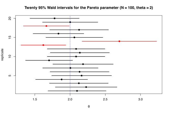
Interpretation.
- The average of the twenty estimates is \(\bar{\hat\theta} = 2.031\), close to the true \(\theta = 2\). The maximum likelihood estimator is in fact slightly biased upwards: \(\sum \log Y_i \sim \text{Gamma}(N, \theta)\), so \(E(\hat\theta) = N\theta/(N-1) = 100 \times 2/99 = 2.0202\) exactly. The observed average sits near that value, as it should. The bias is \(O(1/N)\) and vanishes asymptotically, consistent with the consistency argument in Section 5.4.
- The observed standard deviation of the estimates is \(0.242\), somewhat larger than the asymptotic standard error \(\theta/\sqrt{N} = 0.2\). With only twenty replicates the sample standard deviation itself has a relative standard error of about \(1/\sqrt{2 \times 19} \approx 16\%\), so \(0.242\) is within ordinary sampling noise of \(0.2\).
- Seventeen of the twenty intervals contain \(\theta = 2\) (the three failures, drawn in red in the figure, are replicates 13, 14 and 18). Nominally one expects \(0.95 \times 20 = 19\). Three misses out of twenty is not evidence against the method: under exact 95% coverage the number of misses is \(\text{Bin}(20, 0.05)\), and \(\Pr(\text{3 or more misses}) = 0.075\). A much longer run confirms the interval is behaving as advertised at \(N = 100\):
set.seed(99)
M <- 20000
cover <- replicate(M, { y <- (1/runif(N))^(1/theta); th <- N/sum(log(y))
                        abs(th - theta) <= 1.96*th/sqrt(N) })
mean(cover)
[1] 0.94975
Empirical coverage \(0.94975\) against a nominal \(0.95\) — the Wald interval derived in part (c) is essentially exact at this sample size, so the shortfall in the run of twenty is chance alone.
Problem 5.4 — For the leukemia survival data in Exercise 4.2:
For the leukemia survival data in Exercise 4.2:
a. Use the Wald statistic to obtain an approximate 95% confidence interval for the parameter \(\beta_1\). b. By comparing the deviances for two appropriate models, test the null hypothesis \(\beta_2 = 0\) against the alternative hypothesis \(\beta_2 \neq 0\). What can you conclude about the use of the initial white blood cell count as a predictor of survival time?
(For reference, Exercise 4.2 gives times to death \(y_i\) in weeks from diagnosis and \(\log_{10}\) of the initial white blood cell count \(x_i\), for seventeen patients suffering from leukemia — Example U of Cox and Snell, 1981. Table 4.6 reads: \(y = 65, 156, 100, 134, 16, 108, 121, 4, 39, 143, 56, 26, 22, 1, 1, 5, 65\) with corresponding \(x = 3.36, 2.88, 3.63, 3.41, 3.78, 4.02, 4.00, 4.23, 3.73, 3.85, 3.97, 4.51, 4.54, 5.00, 5.00, 4.72, 5.00\). The model is \(E(Y_i) = \exp(\beta_1 + \beta_2 x_i)\) with \(Y_i\) exponentially distributed, \(f(y; \theta) = \theta e^{-y\theta}\), i.e. a Gamma model with shape parameter \(1\), equivalently dispersion \(\phi = 1\), and a log link.)
(difficulty: \(\star\star\))
The fitted model. Carrying over the fit from Exercise 4.2(d), with the data taken from the dobson package rather than retyped. The one change from Exercise 4.2 is that the standard errors are now computed with the dispersion held at \(\phi = 1\), which is what the exponential distribution asserts; R’s default would estimate \(\phi\) from the Pearson statistic (\(\hat\phi = 0.939\)) and so report slightly smaller standard errors and \(t\) rather than \(z\) statistics. Because the exercise is about the Wald statistic of Equation (5.7), the information must be the one implied by the assumed model, so \(\phi = 1\) is the right choice here.
library(dobson)
data(leukemia)
leuk <- as.data.frame(leukemia)
names(leuk) <- c("y", "x")     # y = survival weeks, x = log10 initial WBC
fit1 <- glm(y ~ x, family = Gamma(link = "log"), data = leuk)
summary(fit1, dispersion = 1)
Call:
glm(formula = y ~ x, family = Gamma(link = "log"), data = leuk)

Coefficients:
            Estimate Std. Error z value Pr(>|z|)
(Intercept)   8.4775     1.6548   5.123 3.01e-07 ***
x            -1.1093     0.3997  -2.776  0.00551 **
---
Signif. codes:  0 '***' 0.001 '**' 0.01 '*' 0.05 '.' 0.1 ' ' 1

(Dispersion parameter for Gamma family taken to be 1)

    Null deviance: 26.282  on 16  degrees of freedom
Residual deviance: 19.457  on 15  degrees of freedom
AIC: 173.97

Number of Fisher Scoring iterations: 8
So \(b_1 = 8.4775\) and \(b_2 = -1.1093\).
a. Wald confidence interval for \(\beta_1\). By Equation (5.8), \(b \sim N(\beta, \mathcal{I}^{-1})\) approximately, so for the single component \(\beta_1\), \[ \frac{b_1 - \beta_1}{\sqrt{(\mathcal{I}^{-1})_{11}}} \sim N(0,1) \quad \Longrightarrow \quad b_1 \pm 1.96 \sqrt{(\mathcal{I}^{-1})_{11}}. \] Here \(\mathcal{I}^{-1} = (X^T W X)^{-1}\) evaluated at the estimates, and \(\sqrt{(\mathcal{I}^{-1})_{11}} = 1.6548\).
b  <- coef(fit1)
se <- sqrt(diag(summary(fit1, dispersion = 1)$cov.scaled))
round(cbind(estimate = b, se = se, lower = b - 1.96*se, upper = b + 1.96*se), 4)
            estimate     se   lower   upper
(Intercept)   8.4775 1.6548  5.2341 11.7209
x            -1.1093 0.3997 -1.8926 -0.3260
The approximate 95% confidence interval for \(\beta_1\) is \[ 8.4775 \pm 1.96 \times 1.6548 = (5.234,\ 11.721). \]
Interpretation. \(\beta_1\) is the value of \(\log E(Y)\) at \(x = 0\), i.e. for a patient with an initial white blood cell count of \(10^0 = 1\). That is a wild extrapolation — the observed \(x\) range is \(2.88\) to \(5.00\) — so the interval is correspondingly wide: back-transformed it says the expected survival of such a hypothetical patient lies between \(e^{5.234} = 188\) weeks and \(e^{11.721} \approx 1.2 \times 10^5\) weeks, around the point estimate \(e^{8.478} \approx 4805\) weeks. The interval is best read as a statement about the intercept of the fitted line on the log scale, not as a clinically meaningful survival prediction. It is nonetheless clearly separated from zero, which merely says that the fitted log-mean is not pinned to the origin. Note also that a Wald interval for \(\beta_1\) alone ignores the strong negative correlation between \(b_1\) and \(b_2\) (the two are nearly collinear because \(x\) is far from \(0\)), so it should not be combined naively with an interval for \(\beta_2\).
b. Deviance test of \(H_0: \beta_2 = 0\). Following Section 5.7, compare two nested models fitted with the same distribution and link:
- \(M_0\): \(E(Y_i) = \exp(\beta_1)\), a single common mean, \(q = 1\) parameter, deviance \(D_0\);
- \(M_1\): \(E(Y_i) = \exp(\beta_1 + \beta_2 x_i)\), \(p = 2\) parameters, deviance \(D_1\).
fit0 <- glm(y ~ 1, family = Gamma(link = "log"), data = leuk)
anova(fit0, fit1, test = "Chisq", dispersion = 1)
Analysis of Deviance Table

Model 1: y ~ 1
Model 2: y ~ x
  Resid. Df Resid. Dev Df Deviance Pr(>Chi)
1        16     26.282
2        15     19.456  1   6.8256 0.008986 **
---
Signif. codes:  0 '***' 0.001 '**' 0.01 '*' 0.05 '.' 0.1 ' ' 1
So \(D_0 = 26.282\) on \(N - q = 16\) degrees of freedom, \(D_1 = 19.456\) on \(N - p = 15\), and \[ \triangle D = D_0 - D_1 = 26.282 - 19.456 = 6.826 \sim \chi^2(p - q) = \chi^2(1) \] under \(H_0\). The 5% critical value is \(\chi^2_{0.95}(1) = 3.841\) and \(6.826 > 3.841\), with \(p = 0.0090\). Reject \(H_0\): \(\beta_2 \neq 0\).
Two remarks on the mechanics. First, no \(F\) ratio is needed here (unlike Section 5.7’s Normal case, where \(\sigma^2\) must be eliminated): the exponential deviance derived in Exercise 5.2 contains no unknown nuisance parameter, so \(\triangle D\) is used directly against \(\chi^2\). Second, if the dispersion is estimated instead of fixed at \(1\), R reports \(p = 0.0070\); the conclusion is unchanged. The Wald test of the same hypothesis from part (a) gives \(z = -2.776\), i.e. \(z^2 = 7.71\) on 1 df (\(p = 0.0055\)) — the same conclusion, and reasonably close to \(\triangle D = 6.83\), as the asymptotic equivalence of the two statistics predicts. The residual deviance \(D_1 = 19.456\) against \(\chi^2(15)\) gives \(p = 0.19\), so there is no evidence that \(M_1\) itself fits badly.
xs <- seq(min(leuk$x), max(leuk$x), length = 200)
p  <- predict(fit1, newdata = data.frame(x = xs), se.fit = TRUE, dispersion = 1)
plot(leuk$x, leuk$y, pch = 19, ylim = c(0, 300),
     xlab = "x = log10(initial white blood cell count)",
     ylab = "y = survival time (weeks)",
     main = "Leukemia survival: exponential model with log link")
lines(xs, exp(p$fit), lwd = 2)
lines(xs, exp(p$fit - 1.96*p$se.fit), lty = 2)
lines(xs, exp(p$fit + 1.96*p$se.fit), lty = 2)
abline(h = mean(leuk$y), col = "grey50", lty = 3)
legend("topright", c("fitted mean", "95% band for the mean", "null model (common mean)"),
       lty = c(1,2,3), lwd = c(2,1,1), col = c("black","black","grey50"), bty = "n")
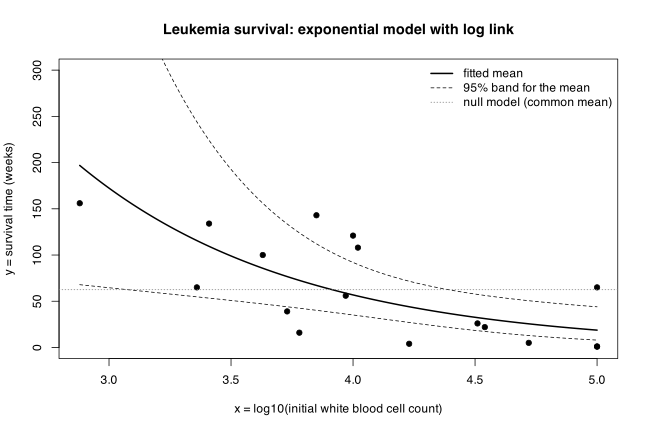
Conclusion about white blood cell count. The initial white blood cell count is a useful predictor of survival time. On the log scale the effect is \(b_2 = -1.109\) with 95% Wald interval \((-1.893, -0.326)\), so a one-unit increase in \(x\) — that is, a tenfold increase in the white blood cell count — multiplies expected survival by \(e^{-1.109} = 0.33\), with 95% interval \((0.15, 0.72)\). Patients presenting with ten times the leukocyte count are expected to survive roughly one third as long, and the data are consistent with anything from a seventh to about three quarters of the survival time. The figure shows the fitted curve falling from about \(200\) weeks at the lowest observed count to under \(20\) weeks at the highest, well outside the flat line of the null model over most of the range.
Two cautions. The evidence rests on 17 observations, so the interval is wide and the tenfold-increase effect is estimated only to within a factor of about five. And the exponential assumption forces \(\operatorname{sd}(Y_i) = E(Y_i)\); Exercise 4.2(e) found this defensible (\(\hat\phi = 0.94\), unstructured Pearson residuals) apart from one long-surviving patient at \(x = 5.00\), which is also the point that most opposes the fitted decline. Dropping it would strengthen, not weaken, the conclusion, so the finding is not an artefact of that observation.
Normal Linear Models
Problem 6.1 — Table 6.22 shows the average apparent per capita consumption of sugar
Table 6.22 shows the average apparent per capita consumption of sugar (in kg per year) in Australia, as refined sugar and in manufactured foods (from Australian Bureau of Statistics, 1998).
Table 6.22 Australian sugar consumption. The columns are period, refined sugar, and sugar in manufactured food: 1936–39, \(32.0\), \(16.3\); 1946–49, \(31.2\), \(23.1\); 1956–59, \(27.0\), \(23.6\); 1966–69, \(21.0\), \(27.7\); 1976–79, \(14.9\), \(34.6\); 1986–89, \(8.8\), \(33.9\).
a. Plot sugar consumption against time separately for refined sugar and sugar in manufactured foods. Fit simple linear regression models to summarize the pattern of consumption of each form of sugar. Calculate 95% confidence intervals for the average annual change in consumption for each form.
b. Calculate the total average sugar consumption for each period and plot these data against time. Using suitable models, test the hypothesis that total sugar consumption did not change over time. (difficulty: \(\star\star\))
Each row is a four-year period, and the periods are spaced exactly ten years apart, so a natural time covariate is the mid-year of each period: \(1937.5, 1947.5, \dots, 1987.5\). Using the mid-year (rather than the row number \(1,\dots,6\)) means the slope is directly interpretable as the average change in consumption per year, which is what part (a) asks for.
The data ship with the dobson package as sugar. One caution: the shipped period label for the second row reads 1046-49, an obvious typo for 1946-49; the numeric columns are correct.
library(dobson)
data(sugar)
sugar <- as.data.frame(sugar)
sugar$period[2] <- "1946-49"   # package ships a typo, 1046-49
sugar$year  <- c(1937.5, 1947.5, 1957.5, 1967.5, 1977.5, 1987.5)
sugar$total <- sugar$refined + sugar$manufactured
sugar
   period refined manufactured   year total
1 1936-39    32.0         16.3 1937.5  48.3
2 1946-49    31.2         23.1 1947.5  54.3
3 1956-59    27.0         23.6 1957.5  50.6
4 1966-69    21.0         27.7 1967.5  48.7
5 1976-79    14.9         34.6 1977.5  49.5
6 1986-89     8.8         33.9 1987.5  42.7
Part (a) — the two forms separately.
par(mfrow = c(1,2), mar = c(4.5,4.5,3,1))
plot(sugar$year, sugar$refined, pch = 16, ylim = c(5,40),
     xlab = "Mid-year of period", ylab = "Consumption (kg/person/year)",
     main = "Refined and manufactured")
abline(lm(refined ~ year, data = sugar), lty = 1)
points(sugar$year, sugar$manufactured, pch = 17, col = "grey40")
abline(lm(manufactured ~ year, data = sugar), lty = 2, col = "grey40")
legend("topright", c("refined","in manufactured food"), pch = c(16,17),
       lty = c(1,2), col = c("black","grey40"), bty = "n")
plot(sugar$year, sugar$total, pch = 16, ylim = c(40,58),
     xlab = "Mid-year of period", ylab = "Total consumption (kg/person/year)",
     main = "Total sugar")
abline(lm(total ~ year, data = sugar), lty = 1)
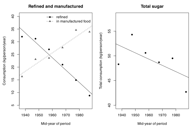
Both series look close to linear in time over this span: refined sugar falls steadily, sugar in manufactured food rises steadily. So the model of Section 6.2, \(E(Y_i) = \beta_0 + \beta_1 x_i\) with \(Y_i \sim N(\mu_i, \sigma^2)\) and \(x_i\) the mid-year, is reasonable for each series.
fit.r <- lm(refined ~ year, data = sugar)
fit.m <- lm(manufactured ~ year, data = sugar)
summary(fit.r)
Call:
lm(formula = refined ~ year, data = sugar)

Residuals:
      1       2       3       4       5       6
-2.6905  1.3924  2.0752  0.9581 -0.2590 -1.4762

Coefficients:
             Estimate Std. Error t value Pr(>|t|)
(Intercept) 980.74405   95.71073   10.25 0.000511 ***
year         -0.48829    0.04877  -10.01 0.000559 ***
---
Signif. codes:  0 ‘***’ 0.001 ‘**’ 0.01 ‘*’ 0.05 ‘.’ 0.1 ‘ ’ 1

Residual standard error: 2.04 on 4 degrees of freedom
Multiple R-squared:  0.9616,	Adjusted R-squared:  0.952
F-statistic: 100.2 on 1 and 4 DF,  p-value: 0.0005593
summary(fit.m)
Call:
lm(formula = manufactured ~ year, data = sugar)

Residuals:
      1       2       3       4       5       6
-1.1905  1.9924 -1.1248 -0.6419  2.6410 -1.6762

Coefficients:
              Estimate Std. Error t value Pr(>|t|)
(Intercept) -683.33095   96.28391  -7.097  0.00208 **
year           0.36171    0.04906   7.373  0.00180 **
---
Signif. codes:  0 ‘***’ 0.001 ‘**’ 0.01 ‘*’ 0.05 ‘.’ 0.1 ‘ ’ 1

Residual standard error: 2.052 on 4 degrees of freedom
Multiple R-squared:  0.9315,	Adjusted R-squared:  0.9143
F-statistic: 54.36 on 1 and 4 DF,  p-value: 0.001804
rbind(refined = confint(fit.r)["year",],
      manufactured = confint(fit.m)["year",])
                  2.5 %     97.5 %
refined      -0.6236872 -0.3528842
manufactured  0.2255019  0.4979267
Interpretation. Refined-sugar consumption fell by an estimated \(0.488\) kg per person per year, 95% CI \((-0.624, -0.353)\); over the half-century covered that is a drop of about \(24\) kg, and the fitted line accounts for \(96\%\) of the variation. Sugar consumed inside manufactured food rose by an estimated \(0.362\) kg per person per year, 95% CI \((0.226, 0.498)\). Neither interval contains zero, so both trends are clearly established. The two slopes are of similar magnitude and opposite sign, which already suggests that the composition of sugar consumption changed — from sugar bought as sugar to sugar bought inside processed food — more than the amount did.
Part (b) — total consumption.
The total is plotted in the right-hand panel above. It hovers near \(50\) kg with no strong trend. To test \(H_0: \beta_1 = 0\) we compare the straight-line model with the intercept-only model \(E(Y_i) = \beta_0\), exactly the deviance comparison of Section 6.2.4: since \(\sigma^2\) is unknown the test statistic is written in terms of residual sums of squares,
\begin{equation*} F = \frac{(S_0 - S_1)/(p - q)}{S_1/(N - p)} \sim F(1, 4) \end{equation*}
under \(H_0\), where \(S_0 = y^T y - b_0^T X_0^T y\) and \(S_1 = y^T y - b_1^T X_1^T y\), with \(q = 1\), \(p = 2\) and \(N = 6\).
fit.t <- lm(total ~ year, data = sugar)
anova(lm(total ~ 1, data = sugar), fit.t)
Analysis of Variance Table

Model 1: total ~ 1
Model 2: total ~ year
  Res.Df    RSS Df Sum of Sq      F Pr(>F)
1      5 71.168
2      4 43.133  1    28.036 2.5999 0.1822
summary(fit.t)$coefficients
confint(fit.t)["year",]
               Estimate   Std. Error   t value  Pr(>|t|)
(Intercept) 297.4130952 154.05674704  1.930542 0.1257369
year         -0.1265714   0.07849728 -1.612431 0.1821628
      2.5 %      97.5 %
-0.34451482  0.09137196
\(F = 2.60\) on \(1\) and \(4\) degrees of freedom, \(p = 0.18\), so the data provide no evidence against the hypothesis that total sugar consumption did not change over time. (Note \(F = t^2\): \((-1.612)^2 = 2.60\), as it must be for a one-degree-of-freedom test.) The point estimate is a decline of \(0.127\) kg per person per year with 95% CI \((-0.345, 0.091)\), so a modest decline is not ruled out — with only \(N = 6\) observations the test has little power. What the analysis does establish firmly is the substitution: total intake changed little while its source shifted decisively from refined sugar to sugar embedded in manufactured food.
Problem 6.2 — Table 6.23 shows response of a grass and legume pasture system to vari-
Table 6.23 shows response of a grass and legume pasture system to various quantities of phosphorus fertilizer (data from D. F. Sinclair; the results were reported in Sinclair and Probert, 1986). The total yield, of grass and legume together, and amount of phosphorus (K) are both given in kilograms per hectare. Find a suitable model for describing the association between yield and quantity of fertilizer.
a. Plot yield against phosphorus to obtain an approximately linear association (you may need to try several transformations of either or both variables in order to achieve approximate linearity).
b. Use the results of (a) to specify a possible model. Fit the model.
c. Calculate the standardized residuals for the model and use appropriate plots to check for any systematic effects that might suggest alternative models and to investigate the validity of any assumptions made.
Table 6.23 Yield of grass and legume pasture and phosphorus levels (K), read as \((K, \text{yield})\) pairs down three columns: \((0, 1753.9)\), \((40, 4923.1)\), \((50, 5246.2)\), \((5, 3184.6)\), \((10, 3538.5)\), \((30, 4000.0)\), \((15, 4184.6)\), \((40, 4692.3)\), \((20, 3600.0)\); \((15, 3107.7)\), \((30, 4415.4)\), \((50, 4938.4)\), \((5, 3046.2)\), \((0, 2553.8)\), \((10, 3323.1)\), \((40, 4461.5)\), \((20, 4215.4)\), \((40, 4153.9)\); \((10, 2400.0)\), \((5, 2861.6)\), \((40, 3723.0)\), \((30, 4892.3)\), \((40, 4784.6)\), \((20, 3184.6)\), \((0, 2723.1)\), \((50, 4784.6)\), \((15, 3169.3)\). (difficulty: \(\star\star\))
Part (a) — finding a linearizing transformation.
Yield should rise with phosphorus but must eventually saturate: soil can only respond so far, so the marginal return per extra kilogram of fertilizer must decline. That is a concave association, and the natural candidates are \(\sqrt{K}\), \(\log(K+1)\) (the shift is needed because \(K = 0\) occurs), or a quadratic in \(K\).
library(dobson)
data(pasture)
pasture <- as.data.frame(pasture)
par(mfrow = c(2,2), mar = c(4.2,4.2,2.5,1))
plot(pasture$K, pasture$yield, pch = 16, xlab = "K (kg/ha)",
     ylab = "Yield (kg/ha)", main = "Untransformed")
plot(sqrt(pasture$K), pasture$yield, pch = 16, xlab = expression(sqrt(K)),
     ylab = "Yield", main = "Square-root of K")
plot(log(pasture$K + 1), pasture$yield, pch = 16, xlab = "log(K+1)",
     ylab = "Yield", main = "log(K+1)")
plot(sqrt(pasture$K), log(pasture$yield), pch = 16, xlab = expression(sqrt(K)),
     ylab = "log(Yield)", main = "log yield vs sqrt K")
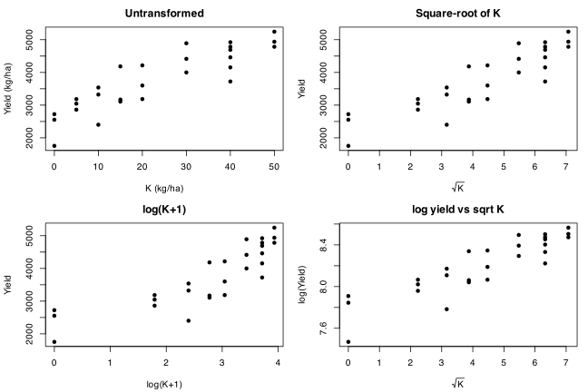
Against raw \(K\) the cloud bends: the jump from \(K=0\) to \(K=10\) is much larger than the jump from \(K=40\) to \(K=50\). Plotting against \(\sqrt{K}\) straightens this out well. The \(\log(K+1)\) scale over-corrects, bunching the high-\(K\) points and leaving \(K=0\) stranded at the left. Transforming the response is not needed — the spread of yields looks roughly constant across \(K\), so there is no variance problem for a log to fix.
Comparing residual sums of squares confirms the visual reading. The last row is fitted on a different response scale, so neither its RSS nor its AIC may be set against the others; only its \(R^2\) is informative.
cand <- list("yield ~ K"        = lm(yield ~ K, data = pasture),
             "yield ~ sqrt(K)"  = lm(yield ~ sqrt(K), data = pasture),
             "yield ~ log(K+1)" = lm(yield ~ log(K + 1), data = pasture),
             "yield ~ K + K^2"  = lm(yield ~ K + I(K^2), data = pasture),
             "log(yield) ~ K"   = lm(log(yield) ~ K, data = pasture))
round(data.frame(RSS = sapply(cand, deviance),
                 R2  = sapply(cand, function(m) summary(m)$r.squared),
                 AIC = sapply(cand, AIC)), 4)
                          RSS     R2      AIC
yield ~ K        4952793.4931 0.7763 409.8526
yield ~ sqrt(K)  4822052.9000 0.7822 409.1303
yield ~ log(K+1) 6465532.7633 0.7080 417.0490
yield ~ K + K^2  4616095.2576 0.7915 409.9517
log(yield) ~ K         0.5135 0.7240 -24.3584
The quadratic buys a slightly smaller RSS but spends an extra parameter for it and has the worse AIC of the two; \(\sqrt{K}\) is the parsimonious choice, and it has the further merit that it is monotone increasing for all \(K\), whereas the fitted quadratic must eventually turn down.
Part (b) — the model.
Take the Normal linear model of equation (6.2),
\begin{equation*} E(Y_i) = \beta_0 + \beta_1 \sqrt{K_i}, \qquad Y_i \sim N(\mu_i, \sigma^2) \ \text{independent}, \end{equation*}
with \(N = 27\) and \(p = 2\).
fit <- lm(yield ~ sqrt(K), data = pasture)
summary(fit)
Call:
lm(formula = yield ~ sqrt(K), data = pasture)

Residuals:
    Min      1Q  Median      3Q     Max
-938.37 -295.34   53.25  327.71  690.59

Coefficients:
            Estimate Std. Error t value Pr(>|t|)
(Intercept)  2159.03     190.10  11.357 2.32e-11 ***
sqrt(K)       372.94      39.35   9.476 9.39e-10 ***
---
Signif. codes:  0 ‘***’ 0.001 ‘**’ 0.01 ‘*’ 0.05 ‘.’ 0.1 ‘ ’ 1

Residual standard error: 439.2 on 25 degrees of freedom
Multiple R-squared:  0.7822,	Adjusted R-squared:  0.7735
F-statistic:  89.8 on 1 and 25 DF,  p-value: 9.386e-10
round(confint(fit), 2)
              2.5 %  97.5 %
(Intercept) 1767.51 2550.55
sqrt(K)      291.89  453.99
Interpretation. With no phosphorus the pasture yields an estimated \(2159\) kg/ha (95% CI \(1768\) to \(2551\)). Yield then grows like \(373\sqrt{K}\): going from \(K=0\) to \(K=10\) adds \(373\sqrt{10} \approx 1179\) kg/ha, whereas going from \(K=40\) to \(K=50\) adds only \(373(\sqrt{50}-\sqrt{40}) \approx 279\) kg/ha. Diminishing returns are exactly what the square root encodes. The residual standard deviation is \(439\) kg/ha, about \(10\%\) of a typical yield.
Part (c) — standardized residuals and diagnostics.
Standardized residuals are those of Section 6.2.6, \(r_i = (y_i - \hat\mu_i)/\{\hat\sigma\sqrt{1 - h_{ii}}\}\), obtained in R with rstandard.
r <- rstandard(fit)
par(mfrow = c(2,2), mar = c(4.2,4.2,2.5,1))
plot(fitted(fit), r, pch = 16, xlab = "Fitted yield",
     ylab = "Standardised residual", main = "Residuals vs fitted"); abline(h = 0, lty = 2)
plot(pasture$K, r, pch = 16, xlab = "K (kg/ha)",
     ylab = "Standardised residual", main = "Residuals vs K"); abline(h = 0, lty = 2)
qqnorm(r, pch = 16, main = "Normal Q-Q"); qqline(r)
plot(seq_along(r), r, type = "b", pch = 16, xlab = "Observation order",
     ylab = "Standardised residual", main = "Residuals in data order"); abline(h = 0, lty = 2)
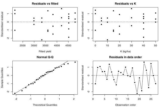
The residuals scatter about zero with no funnel against the fitted values (homoscedasticity is tenable) and no curvature against \(K\) — had a \(\sqrt{K}\) term been the wrong bend, the residuals would arch or sag across the \(K\) range. The Q-Q plot is close to the line.
Because \(K\) takes only eight distinct levels with replication, a formal lack-of-fit test is available: compare the fitted straight line with the saturated one-way model that gives every level of \(K\) its own mean. The extra sum of squares measures curvature not captured by \(\sqrt{K}\), and the denominator is pure error.
anova(fit, lm(yield ~ factor(K), data = pasture))
Analysis of Variance Table

Model 1: yield ~ sqrt(K)
Model 2: yield ~ factor(K)
  Res.Df     RSS Df Sum of Sq      F Pr(>F)
1     25 4822053
2     19 4109224  6    712829 0.5493 0.7645
shapiro.test(rstandard(fit))
	Shapiro-Wilk normality test

data:  rstandard(fit)
W = 0.96755, p-value = 0.5384
\(F = 0.55\) on \(6\) and \(19\) degrees of freedom (\(p = 0.76\)): no detectable systematic departure from the square-root curve, so nothing is left for a more elaborate model to explain. Normality is not contradicted (\(p = 0.54\)). The model
\begin{equation*} \widehat{\text{yield}} = 2159 + 373\sqrt{K} \end{equation*}
is an adequate summary of the fertilizer response.
Problem 6.3 — Analyze the carbohydrate data in Table 6.3 using appropriate software (or,
Analyze the carbohydrate data in Table 6.3 using appropriate software (or, preferably, repeat the analyses using several different regression programs and compare the results).
a. Plot the responses \(y\) against each of the explanatory variables \(x_1\), \(x_2\) and \(x_3\) to see if \(y\) appears to be linearly related to them.
b. Fit the Model (6.6) and examine the residuals to assess the adequacy of the model and the assumptions.
c. Fit the models \[ E(Y_i) = \beta_0 + \beta_1 x_{i1} + \beta_3 x_{i3} \] and \[ E(Y_i) = \beta_0 + \beta_3 x_{i3} \] (note the variable \(x_2\), relative weight, is omitted from both models), and use these to test the hypothesis: \(\beta_1 = 0\). Compare your results with Table 6.5.
Table 6.3 gives, for twenty male insulin-dependent diabetics, carbohydrate \(y\) (percentage of total calories from complex carbohydrates), age \(x_1\) (years), relative weight \(x_2\) and protein \(x_3\) (percentage of calories), as rows \((y, x_1, x_2, x_3)\): \((33,33,100,14)\), \((40,47,92,15)\), \((37,49,135,18)\), \((27,35,144,12)\), \((30,46,140,15)\), \((43,52,101,15)\), \((34,62,95,14)\), \((48,23,101,17)\), \((30,32,98,15)\), \((38,42,105,14)\), \((50,31,108,17)\), \((51,61,85,19)\), \((30,63,130,19)\), \((36,40,127,20)\), \((41,50,109,15)\), \((42,64,107,16)\), \((46,56,117,18)\), \((24,61,100,13)\), \((35,48,118,18)\), \((37,28,102,14)\). (difficulty: \(\star\star\))
Part (a) — marginal plots.
library(dobson)
data(carbohydrate)
carbohydrate <- as.data.frame(carbohydrate)
par(mfrow = c(1,3), mar = c(4.5,4.5,3,1))
for (v in c("age","weight","protein")) {
  plot(carbohydrate[[v]], carbohydrate$carbohydrate, pch = 16, xlab = v,
       ylab = "Carbohydrate (% of calories)", main = paste("y vs", v))
  abline(lm(carbohydrate$carbohydrate ~ carbohydrate[[v]]), lty = 2)
}
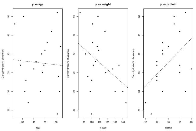
round(cor(carbohydrate), 3)
             carbohydrate    age weight protein
carbohydrate        1.000 -0.059 -0.407   0.463
age                -0.059  1.000 -0.043   0.193
weight             -0.407 -0.043  1.000   0.147
protein             0.463  0.193  0.147   1.000
Marginally, \(y\) shows essentially no association with age (\(r = -0.06\)), a moderate negative association with relative weight (\(r = -0.41\)) and a moderate positive one with protein (\(r = 0.46\)). In each panel a straight line is a defensible summary — no curvature is apparent, though with \(N = 20\) and this much scatter mild curvature would be hard to see. The explanatory variables are only weakly correlated with one another (largest \(|r| = 0.19\)), so the design is close to, but not exactly, orthogonal — which is what part (c) probes.
Part (b) — Model (6.6) and its residuals.
m66 <- lm(carbohydrate ~ age + weight + protein, data = carbohydrate)
summary(m66)
Call:
lm(formula = carbohydrate ~ age + weight + protein, data = carbohydrate)

Residuals:
     Min       1Q   Median       3Q      Max
-10.3424  -4.8203   0.9897   3.8553   7.9087

Coefficients:
            Estimate Std. Error t value Pr(>|t|)
(Intercept) 36.96006   13.07128   2.828  0.01213 *
age         -0.11368    0.10933  -1.040  0.31389
weight      -0.22802    0.08329  -2.738  0.01460 *
protein      1.95771    0.63489   3.084  0.00712 **
---
Signif. codes:  0 ‘***’ 0.001 ‘**’ 0.01 ‘*’ 0.05 ‘.’ 0.1 ‘ ’ 1

Residual standard error: 5.956 on 16 degrees of freedom
Multiple R-squared:  0.4805,	Adjusted R-squared:  0.3831
F-statistic: 4.934 on 3 and 16 DF,  p-value: 0.01297
This reproduces the book exactly: \(b = (36.960, -0.114, -0.228, 1.958)^T\) and the standard errors of Table 6.4, with residual sum of squares \(567.663\) on \(16\) degrees of freedom and \(\hat\sigma^2 = 35.48\).
par(mfrow = c(2,2), mar = c(4.2,4.2,2.5,1))
plot(m66, which = 1:4)
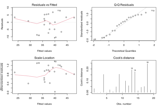
round(data.frame(y = carbohydrate$carbohydrate, fitted = fitted(m66),
                 std.res = rstandard(m66), leverage = hatvalues(m66),
                 cooks = cooks.distance(m66)), 3)
    y fitted std.res leverage cooks
1  33 37.815  -0.876    0.148 0.033
2  40 40.005  -0.001    0.120 0.000
3  37 35.846   0.215    0.192 0.003
4  27 23.639   0.794    0.495 0.154
5  30 29.174   0.159    0.239 0.002
6  43 37.385   0.987    0.087 0.023
7  34 35.658  -0.316    0.224 0.007
8  48 44.597   0.681    0.296 0.049
9  30 40.342  -1.883    0.149 0.156
10 38 35.652   0.414    0.093 0.004
11 50 42.091   1.448    0.159 0.099
12 51 47.841   0.658    0.349 0.058
13 30 37.353  -1.445    0.270 0.193
14 36 42.609  -1.317    0.290 0.177
15 41 35.788   0.906    0.067 0.015
16 42 36.610   0.985    0.156 0.045
17 46 39.155   1.225    0.120 0.051
18 24 32.674  -1.688    0.256 0.245
19 35 39.836  -0.857    0.102 0.021
20 37 37.927  -0.173    0.188 0.002
This is Table 6.6 and Figure 6.1 of the text. Reading the diagnostics:
- Residuals versus fitted values show no trend and no funnel, so linearity in the mean and constant variance are tenable.
- The standardized residuals all lie inside \((-1.9, 1.5)\); for \(N = 20\) that is entirely unremarkable, and the Q-Q plot is close to straight, so Normality is not contradicted.
- Observation 4 has by far the largest leverage, \(h_{44} = 0.495\) (against the average \(p/N = 0.2\)). It is the subject with the highest relative weight (\(144\)) and the lowest protein (\(12\)), so it sits at the edge of the covariate space. But its residual is small, so its Cook’s distance is only \(0.154\).
- The largest Cook’s distance anywhere is \(0.245\) (observation 18), far below the conventional value of \(1\) that would flag undue influence.
As the text says, there is little evidence against the assumptions and no unduly influential observation. Model (6.6) is adequate.
Part (c) — testing \(\beta_1 = 0\) with \(x_2\) omitted.
m13 <- lm(carbohydrate ~ age + protein, data = carbohydrate)
m3  <- lm(carbohydrate ~ protein, data = carbohydrate)
anova(m3, m13)
Analysis of Variance Table

Model 1: carbohydrate ~ protein
Model 2: carbohydrate ~ age + protein
  Res.Df    RSS Df Sum of Sq      F Pr(>F)
1     18 858.65
2     17 833.57  1    25.079 0.5115 0.4842
The improvement due to adding age when only protein is in the model is \(858.650 - 833.571 = 25.079\), and
\begin{equation*} F = \frac{25.079/1}{833.571/17} = \frac{25.079}{49.033} = 0.51 \sim F(1,17), \end{equation*}
which is not significant (\(p = 0.48\)). The conclusion — no evidence that carbohydrate depends on age — agrees with the text.
The numbers, however, do not agree with Table 6.5. There, with weight in the model, the improvement due to age was \(606.022 - 567.663 = 38.359\) and \(F = 38.359/35.489 = 1.08\) on \(1\) and \(16\) degrees of freedom:
anova(lm(carbohydrate ~ weight + protein, data = carbohydrate), m66)
Analysis of Variance Table

Model 1: carbohydrate ~ weight + protein
Model 2: carbohydrate ~ age + weight + protein
  Res.Df    RSS Df Sum of Sq      F Pr(>F)
1     17 606.02
2     16 567.66  1    38.359 1.0812 0.3139
So the sum of squares attributable to age is \(25.079\) when weight is absent but \(38.359\) when weight is present, and the residual mean square drops from \(49.03\) to \(35.49\) once weight is included. Both the numerator and the denominator of the \(F\) ratio change.
This is the lack of orthogonality discussed in Section 6.2.5. Were \(X\) orthogonal, \(X^T X\) would be block diagonal, the estimate \(b_1\) and its sum of squares would not depend on which other columns were in the model, and the two ANOVA tables would agree. Here the columns for age, weight and protein are not mutually orthogonal (age and protein correlate at \(r = 0.19\), weight and protein at \(r = 0.15\)), so the contribution of age is not a fixed quantity — it depends on the order of fitting. The estimated protein coefficient shows the same effect: \(1.958\) in Model (6.6) but \(1.682\) in the model without weight. The practical lesson is that in observational data a “sum of squares for age” has no meaning on its own; one must say what else was in the model.
Problem 6.4 — It is well known that the concentration of cholesterol in blood serum in-
It is well known that the concentration of cholesterol in blood serum increases with age, but it is less clear whether cholesterol level is also associated with body weight. Table 6.24 shows for thirty women serum cholesterol (millimoles per liter), age (years) and body mass index (weight divided by height squared, where weight was measured in kilograms and height in meters). Use multiple regression to test whether serum cholesterol is associated with body mass index when age is already included in the model.
Table 6.24 Cholesterol (CHOL), age and body mass index (BMI) for thirty women, as triples \((\text{CHOL}, \text{Age}, \text{BMI})\): \((5.94,52,20.7)\), \((4.71,46,21.3)\), \((5.86,51,25.4)\), \((6.52,44,22.7)\), \((6.80,70,23.9)\), \((5.23,33,24.3)\), \((4.97,21,22.2)\), \((8.78,63,26.2)\), \((5.13,56,23.3)\), \((6.74,54,29.2)\), \((5.95,44,22.7)\), \((5.83,71,21.9)\), \((5.74,39,22.4)\), \((4.92,58,20.2)\), \((6.69,58,24.4)\), \((6.48,65,26.3)\), \((8.83,76,22.7)\), \((5.10,47,21.5)\), \((5.81,43,20.7)\), \((4.65,30,18.9)\), \((6.82,58,23.9)\), \((6.28,78,24.3)\), \((5.15,49,23.8)\), \((2.92,36,19.6)\), \((9.27,67,24.3)\), \((5.57,42,22.0)\), \((4.92,29,22.5)\), \((6.72,33,24.1)\), \((5.57,42,22.7)\), \((6.25,66,27.3)\). (difficulty: \(\star\star\))
The question is explicitly a conditional one: does BMI add anything once age is in the model? That is a comparison of two nested Normal linear models,
\begin{equation*} M_1: \ E(Y_i) = \beta_0 + \beta_1 \text{age}_i, \qquad M_2: \ E(Y_i) = \beta_0 + \beta_1 \text{age}_i + \beta_2 \text{BMI}_i, \end{equation*}
with \(Y_i \sim N(\mu_i, \sigma^2)\), tested by \(H_0: \beta_2 = 0\) using the \(F\) statistic of Section 6.2.4.
library(dobson)
data(cholesterol)
chol <- as.data.frame(cholesterol)
par(mfrow = c(1,3), mar = c(4.5,4.5,3,1))
plot(chol$age, chol$chol, pch = 16, xlab = "Age (years)",
     ylab = "Serum cholesterol (mmol/l)", main = "CHOL vs age")
abline(lm(chol ~ age, data = chol), lty = 2)
plot(chol$bmi, chol$chol, pch = 16, xlab = "BMI (kg/m^2)",
     ylab = "Serum cholesterol (mmol/l)", main = "CHOL vs BMI")
abline(lm(chol ~ bmi, data = chol), lty = 2)
plot(chol$age, chol$bmi, pch = 16, xlab = "Age (years)",
     ylab = "BMI (kg/m^2)", main = "BMI vs age")
abline(lm(bmi ~ age, data = chol), lty = 2)
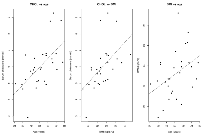
round(cor(chol), 3)
      chol   age   bmi
chol 1.000 0.603 0.535
age  0.603 1.000 0.403
bmi  0.535 0.403 1.000
The third panel is the reason the question is worth asking: age and BMI are themselves correlated (\(r = 0.40\)), so the marginal association between cholesterol and BMI (\(r = 0.54\)) is partly borrowed from age. Only a multiple regression separates them.
m1 <- lm(chol ~ age, data = chol)
m2 <- lm(chol ~ age + bmi, data = chol)
summary(m1)
Call:
lm(formula = chol ~ age, data = chol)

Residuals:
     Min       1Q   Median       3Q      Max
-2.29944 -0.67361  0.02992  0.40873  2.39393

Coefficients:
            Estimate Std. Error t value Pr(>|t|)
(Intercept)  3.29561    0.70480   4.676 6.72e-05 ***
age          0.05344    0.01336   3.999 0.000422 ***
---
Signif. codes:  0 ‘***’ 0.001 ‘**’ 0.01 ‘*’ 0.05 ‘.’ 0.1 ‘ ’ 1

Residual standard error: 1.063 on 28 degrees of freedom
Multiple R-squared:  0.3635,	Adjusted R-squared:  0.3408
F-statistic: 15.99 on 1 and 28 DF,  p-value: 0.0004216
summary(m2)
Call:
lm(formula = chol ~ age + bmi, data = chol)

Residuals:
    Min      1Q  Median      3Q     Max
-1.7619 -0.7353 -0.0205  0.3772  2.3717

Coefficients:
            Estimate Std. Error t value Pr(>|t|)
(Intercept) -0.73983    1.89641  -0.390  0.69951
age          0.04097    0.01363   3.006  0.00567 **
bmi          0.20137    0.08876   2.269  0.03149 *
---
Signif. codes:  0 ‘***’ 0.001 ‘**’ 0.01 ‘*’ 0.05 ‘.’ 0.1 ‘ ’ 1

Residual standard error: 0.992 on 27 degrees of freedom
Multiple R-squared:  0.4654,	Adjusted R-squared:  0.4258
F-statistic: 11.75 on 2 and 27 DF,  p-value: 0.000213
anova(m1, m2)
Analysis of Variance Table

Model 1: chol ~ age
Model 2: chol ~ age + bmi
  Res.Df    RSS Df Sum of Sq      F  Pr(>F)
1     28 31.636
2     27 26.571  1    5.0655 5.1474 0.03149 *
---
Signif. codes:  0 ‘***’ 0.001 ‘**’ 0.01 ‘*’ 0.05 ‘.’ 0.1 ‘ ’ 1
round(confint(m2), 4)
              2.5 % 97.5 %
(Intercept) -4.6309 3.1513
age          0.0130 0.0689
bmi          0.0193 0.3835
The test. Adding BMI to the age-only model reduces the residual sum of squares from \(31.636\) to \(26.571\), an improvement of \(5.066\) on one degree of freedom. With \(\hat\sigma^2 = 26.571/27 = 0.984\),
\begin{equation*} F = \frac{5.066/1}{26.571/27} = 5.15 \sim F(1, 27) \ \text{under} \ H_0, \end{equation*}
giving \(p = 0.031\). (Equivalently \(t = 2.269\) on the BMI coefficient, and \(t^2 = 5.15\).) At the \(5\%\) level we reject \(H_0: \beta_2 = 0\): serum cholesterol is associated with body mass index after adjusting for age.
Interpretation. Holding age fixed, each additional unit of BMI (one \(\text{kg}/\text{m}^2\)) is associated with a \(0.201\) mmol/l higher serum cholesterol, 95% CI \((0.019, 0.384)\). The interval is wide and only just clears zero, so the evidence is suggestive rather than decisive with \(N = 30\). Note the shrinkage from the unadjusted BMI slope of \(0.309\) to the adjusted \(0.201\): about a third of the apparent BMI effect is really age acting through the age–BMI correlation. Age itself stays significant after adjustment (\(0.041\) mmol/l per year, \(p = 0.006\)), confirming the well-known age effect. Together the two covariates explain \(47\%\) of the variance in cholesterol.
Checking the model.
par(mfrow = c(2,2), mar = c(4.2,4.2,2.5,1))
plot(m2, which = 1:4)
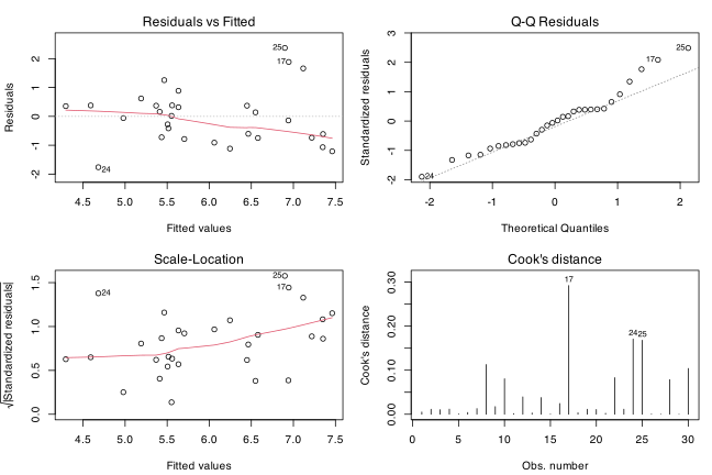
round(head(sort(cooks.distance(m2), decreasing = TRUE), 4), 3)
anova(m2, lm(chol ~ age * bmi, data = chol))
   17    24    25     8
0.292 0.171 0.168 0.113

Analysis of Variance Table

Model 1: chol ~ age + bmi
Model 2: chol ~ age * bmi
  Res.Df    RSS Df Sum of Sq      F Pr(>F)
1     27 26.571
2     26 26.127  1   0.44352 0.4414 0.5123
Residuals show no pattern against fitted values and follow the Normal Q-Q line reasonably; the largest Cook’s distance is \(0.29\) (woman 17, aged \(76\) with a high cholesterol of \(8.83\) but only average BMI), well short of the value \(1\) that would indicate a single observation driving the conclusion. Adding an age-by-BMI interaction gives \(F = 0.44\), \(p = 0.51\), so there is no evidence that the BMI effect differs with age; the additive model is adequate.
One caveat worth stating: with \(p = 0.031\) the finding is not robust to much. Dropping the most influential observation, or a slightly different transformation of BMI, could easily move the \(p\)-value across \(0.05\). The honest summary is that these data give moderate — not strong — evidence for a BMI effect independent of age.
Problem 6.5 — Table 6.25 shows plasma inorganic phosphate levels (mg/dl) one hour af-
Table 6.25 shows plasma inorganic phosphate levels (mg/dl) one hour after a standard glucose tolerance test for obese subjects, with or without hyperinsulinemia, and controls (data from Jones, 1987).
Table 6.25 Plasma phosphate levels in obese and control subjects. Hyperinsulinemic obese (\(n = 11\)): \(2.3, 4.1, 4.2, 4.0, 4.6, 4.6, 3.8, 5.2, 3.1, 3.7, 3.8\). Non-hyperinsulinemic obese (\(n = 8\)): \(3.0, 4.1, 3.9, 3.1, 3.3, 2.9, 3.3, 3.9\). Controls (\(n = 12\)): \(3.0, 2.6, 3.1, 2.2, 2.1, 2.4, 2.8, 3.4, 2.9, 2.6, 3.1, 3.2\).
a. Perform a one-factor analysis of variance to test the hypothesis that there are no mean differences among the three groups. What conclusions can you draw?
b. Obtain a 95% confidence interval for the difference in means between the two obese groups.
c. Using an appropriate model, examine the standardized residuals for all the observations to look for any systematic effects and to check the Normality assumption. (difficulty: \(\star\star\))
This is the one-factor analysis of variance of Section 6.4.1, with \(J = 3\) groups of unequal sizes \(n_1 = 12\), \(n_2 = 8\), \(n_3 = 11\) and \(N = 31\). The model is
\begin{equation*} E(Y_{jk}) = \mu + \alpha_j, \qquad Y_{jk} \sim N(\mu + \alpha_j, \sigma^2), \end{equation*}
\(j = 1,2,3\), with the corner-point constraint \(\alpha_1 = 0\) (controls as reference). The null hypothesis is \(H_0: \alpha_1 = \alpha_2 = \alpha_3\), equivalently \(E(Y_{jk}) = \mu\) for all groups.
library(dobson)
data(plasma)
pl <- as.data.frame(plasma)
pl$Group <- factor(pl$Group, levels = c("C","N-O","H-O"),
                   labels = c("control","non-hyperinsulinemic obese",
                              "hyperinsulinemic obese"))
aggregate(phosphate ~ Group, data = pl,
          function(z) c(n = length(z), mean = round(mean(z),3), sd = round(sd(z),3)))
                       Group phosphate.n phosphate.mean phosphate.sd
1                    control      12.000          2.783        0.409
2 non-hyperinsulinemic obese       8.000          3.438        0.463
3     hyperinsulinemic obese      11.000          3.945        0.778
Part (a) — the analysis of variance.
fit <- lm(phosphate ~ Group, data = pl)
anova(fit)
Analysis of Variance Table

Response: phosphate
          Df Sum Sq Mean Sq F value    Pr(>F)
Group      2 7.8083  3.9041  11.651 0.0002082 ***
Residuals 28 9.3827  0.3351
---
Signif. codes:  0 ‘***’ 0.001 ‘**’ 0.01 ‘*’ 0.05 ‘.’ 0.1 ‘ ’ 1
summary(fit)
Call:
lm(formula = phosphate ~ Group, data = pl)

Residuals:
     Min       1Q   Median       3Q      Max
-1.64545 -0.29148  0.01667  0.36667  1.25455

Coefficients:
                                Estimate Std. Error t value Pr(>|t|)
(Intercept)                       2.7833     0.1671  16.656 4.63e-16 ***
Groupnon-hyperinsulinemic obese   0.6542     0.2642   2.476   0.0196 *
Grouphyperinsulinemic obese       1.1621     0.2416   4.809 4.67e-05 ***
---
Signif. codes:  0 ‘***’ 0.001 ‘**’ 0.01 ‘*’ 0.05 ‘.’ 0.1 ‘ ’ 1

Residual standard error: 0.5789 on 28 degrees of freedom
Multiple R-squared:  0.4542,	Adjusted R-squared:  0.4152
F-statistic: 11.65 on 2 and 28 DF,  p-value: 0.0002082
The between-groups sum of squares is \(7.808\) on \(2\) degrees of freedom and the residual sum of squares \(9.383\) on \(28\), so
\begin{equation*} F = \frac{7.8083/2}{9.3827/28} = \frac{3.904}{0.335} = 11.65 \sim F(2,28) \end{equation*}
under \(H_0\), with \(p = 0.0002\). We reject \(H_0\) decisively: mean plasma phosphate differs among the three groups.
Conclusions. Group means run in a clear ordering, controls \(2.78 <\) non-hyperinsulinemic obese \(3.44 <\) hyperinsulinemic obese \(3.94\) mg/dl. Both obese groups sit above the controls: \(+0.65\) mg/dl (95% CI \(0.11\) to \(1.20\)) for the non-hyperinsulinemic and \(+1.16\) mg/dl (95% CI \(0.67\) to \(1.66\)) for the hyperinsulinemic. Group membership accounts for \(45\%\) of the variance. So obesity is associated with higher post-glucose-load phosphate, and hyperinsulinemia appears to raise it further still — although part (b) shows the second step is less well established than the first.
Part (b) — difference between the two obese groups.
The contrast is \(\alpha_3 - \alpha_2\), with estimated standard error \(\hat\sigma\sqrt{1/n_2 + 1/n_3}\) from the pooled residual mean square.
s2 <- summary(fit)$sigma^2
n2 <- 8; n3 <- 11
d  <- diff(tapply(pl$phosphate, pl$Group, mean)[2:3])
se <- sqrt(s2 * (1/n2 + 1/n3))
tc <- qt(0.975, df.residual(fit))
round(c(difference = unname(d), se = se,
        lower = unname(d) - tc*se, upper = unname(d) + tc*se), 4)
difference         se      lower      upper
    0.5080     0.2690    -0.0430     1.0589
The hyperinsulinemic obese average \(0.508\) mg/dl higher than the non-hyperinsulinemic obese, 95% CI \((-0.043, 1.059)\). The interval just includes zero, so on these data the two obese groups are not significantly different from one another at the \(5\%\) level (\(t = 1.89\), \(p = 0.069\)). The overall \(F\) test is driven mainly by the contrast between obese subjects and controls; whether hyperinsulinemia adds a further increment is left unsettled by a sample of \(8\) and \(11\).
Note that this interval uses the pooled \(\hat\sigma^2 = 0.335\) on \(28\) degrees of freedom, borrowing information from the control group, which is legitimate only under the equal-variance assumption checked in part (c). It is also a single pre-specified comparison, so no multiplicity adjustment is applied; had all three pairwise comparisons been made post hoc, a Tukey correction would widen it.
Part (c) — residuals.
For the one-factor model the fitted value is the group mean, so the residuals \(y_{jk} - \bar y_j\) carry all the information about within-group behaviour. Standardized residuals \(r_i = (y_i - \hat\mu_i)/\{\hat\sigma\sqrt{1-h_{ii}}\}\) are used, as in Section 6.2.6.
par(mfrow = c(2,2), mar = c(4.2,4.2,2.5,1))
boxplot(phosphate ~ Group, data = pl, ylab = "Plasma phosphate (mg/dl)",
        names = c("control","non-hyp.","hyper."), main = "Group distributions")
stripchart(phosphate ~ Group, data = pl, vertical = TRUE, add = TRUE,
           pch = 16, col = "grey30", method = "jitter", jitter = 0.08)
r <- rstandard(fit)
plot(fitted(fit), r, pch = 16, xlab = "Fitted (group mean)",
     ylab = "Standardised residual", main = "Residuals vs fitted"); abline(h = 0, lty = 2)
qqnorm(r, pch = 16, main = "Normal Q-Q"); qqline(r)
plot(seq_along(r), r, pch = 16, xlab = "Observation index",
     ylab = "Standardised residual", main = "Residuals in order"); abline(h = 0, lty = 2)
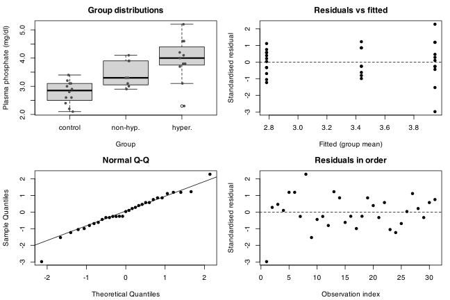
bartlett.test(phosphate ~ Group, data = pl)
shapiro.test(rstandard(fit))
round(sort(rstandard(fit))[1:3], 3)
	Bartlett test of homogeneity of variances

data:  phosphate by Group
Bartlett's K-squared = 4.663, df = 2, p-value = 0.09715

	Shapiro-Wilk normality test

data:  rstandard(fit)
W = 0.96994, p-value = 0.5174

     1      9     24
-2.981 -1.532 -1.233
Reading the plots:
- The residuals-versus-fitted panel shows the group with the largest mean (hyperinsulinemic obese) also has the widest spread: within-group standard deviations are \(0.41\), \(0.46\), \(0.78\). Bartlett’s test gives \(p = 0.097\), so the departure from equal variances is not formally significant, but it is the one visible systematic effect and it does put mild strain on the pooled-variance interval of part (b).
- The Normal Q-Q plot is straight except for one point at the bottom left. That is observation 1, the hyperinsulinemic subject with phosphate \(2.3\): its standardized residual is \(-2.98\), an outlier by any reading, and it is what inflates the third group’s variance. Shapiro–Wilk on all \(31\) residuals gives \(p = 0.52\), so Normality is not rejected overall, but the single low value is worth flagging — excluding it would sharpen the obese-group contrast rather than weaken it.
- There is no trend against observation index, consistent with independence.
Overall the one-factor Normal model is acceptable. The conclusions are safe for the obese-versus-control contrast; the hyperinsulinemic-versus-non-hyperinsulinemic comparison depends on the one aberrant low reading and on the equal-variance assumption, and should be treated as provisional.
Problem 6.6 — The weights (in grams) of machine components of a standard size made
The weights (in grams) of machine components of a standard size made by four different workers on two different days are shown in Table 6.26; five components were chosen randomly from the output of each worker on each day. Perform an analysis of variance to test for differences among workers, among days, and possible interaction effects. What are your conclusions?
Table 6.26 Weights of machine components made by workers on different days. Day 1, worker 1: \(35.7, 37.1, 36.7, 37.7, 35.3\); worker 2: \(38.4, 37.2, 38.1, 36.9, 37.2\); worker 3: \(34.9, 34.3, 34.5, 33.7, 36.2\); worker 4: \(37.1, 35.5, 36.5, 36.0, 33.8\). Day 2, worker 1: \(34.7, 35.2, 34.6, 36.4, 35.2\); worker 2: \(36.9, 38.5, 36.4, 37.8, 36.1\); worker 3: \(32.0, 35.2, 33.5, 32.9, 33.3\); worker 4: \(35.8, 32.9, 35.7, 38.0, 36.1\). (difficulty: \(\star\star\))
This is the balanced two-factor analysis of variance of Section 6.4.2, with factor A = worker (\(J = 4\)), factor B = day (\(K = 2\)) and \(L = 5\) replicates in each of the \(JK = 8\) subgroups, so \(N = 40\). Following the chapter we fit the saturated Model (6.9) and the reduced Models (6.10) to (6.12) with corner-point constraints, and compare them by \(F\) tests on the differences in scaled deviance \(\sigma^2 D = y^T y - b^T X^T y\).
Two data-entry faults in the dobson package copy of this table must be repaired first: four all-missing rows are appended (rows 41–44), and the second day-2 measurement for worker 4 is recorded as \(332.9\) where Table 6.26 prints \(32.9\). After the repair the design is balanced at \(5\) per cell, as it should be.
library(dobson)
data(machine)
mc <- as.data.frame(machine)
mc <- mc[!is.na(mc$weight), ]      # drop 4 empty rows shipped in the package
mc$weight[mc$weight > 100] <- 32.9 # 332.9 is a typo for 32.9
mc$day <- factor(mc$day); mc$worker <- factor(mc$worker)
tapply(mc$weight, list(mc$day, mc$worker), mean)
      1     2     3     4
1 36.50 37.56 34.72 35.78
2 35.22 37.14 33.38 35.70
The sequence of model comparisons.
sat <- lm(weight ~ day * worker, data = mc)   # Model (6.9)
add <- lm(weight ~ day + worker, data = mc)   # Model (6.10)
mW  <- lm(weight ~ worker, data = mc)         # Model (6.11), B omitted
mD  <- lm(weight ~ day, data = mc)            # Model (6.12), A omitted
anova(add, sat)
Analysis of Variance Table

Model 1: weight ~ day + worker
Model 2: weight ~ day * worker
  Res.Df    RSS Df Sum of Sq     F Pr(>F)
1     35 43.154
2     32 40.196  3     2.958 0.785 0.5112
\(H_I\) (no interaction): \(F = (2.958/3)/(40.196/32) = 0.79\) on \(3\) and \(32\) degrees of freedom, \(p = 0.51\). No evidence of interaction — the difference between the two days is the same for every worker, at least to the resolution of these data. Since \(H_I\) is not rejected we proceed to the main effects.
anova(mW, add) # HB: no day effect
Analysis of Variance Table

Model 1: weight ~ worker
Model 2: weight ~ day + worker
  Res.Df    RSS Df Sum of Sq      F  Pr(>F)
1     36 49.238
2     35 43.154  1     6.084 4.9344 0.03289 *
---
Signif. codes:  0 ‘***’ 0.001 ‘**’ 0.01 ‘*’ 0.05 ‘.’ 0.1 ‘ ’ 1
anova(mD, add) # HA: no worker effect
Analysis of Variance Table

Model 1: weight ~ day
Model 2: weight ~ day + worker
  Res.Df    RSS Df Sum of Sq      F    Pr(>F)
1     38 97.776
2     35 43.154  3    54.622 14.767 2.236e-06 ***
---
Signif. codes:  0 ‘***’ 0.001 ‘**’ 0.01 ‘*’ 0.05 ‘.’ 0.1 ‘ ’ 1
The full ANOVA table collects all of this. Because the design is balanced, \(X\) can be made orthogonal (Section 6.2.5), so these sums of squares do not depend on the order of fitting — the sequential table below and the model comparisons above give identical numerators.
anova(sat)
Analysis of Variance Table

Response: weight
           Df Sum Sq Mean Sq F value    Pr(>F)
day         1  6.084  6.0840  4.8435   0.03508 *
worker      3 54.622 18.2073 14.4948 3.895e-06 ***
day:worker  3  2.958  0.9860  0.7850   0.51117
Residuals  32 40.196  1.2561
---
Signif. codes:  0 ‘***’ 0.001 ‘**’ 0.01 ‘*’ 0.05 ‘.’ 0.1 ‘ ’ 1
The fitted additive model.
summary(add)
Call:
lm(formula = weight ~ day + worker, data = mc)

Residuals:
    Min      1Q  Median      3Q     Max
-2.4500 -0.6575 -0.1350  0.6825  2.6500

Coefficients:
            Estimate Std. Error t value Pr(>|t|)
(Intercept)  36.2500     0.3926  92.337  < 2e-16 ***
day2         -0.7800     0.3511  -2.221  0.03289 *
worker2       1.4900     0.4966   3.001  0.00494 **
worker3      -1.8100     0.4966  -3.645  0.00086 ***
worker4      -0.1200     0.4966  -0.242  0.81046
---
Signif. codes:  0 ‘***’ 0.001 ‘**’ 0.01 ‘*’ 0.05 ‘.’ 0.1 ‘ ’ 1

Residual standard error: 1.11 on 35 degrees of freedom
Multiple R-squared:  0.5845,	Adjusted R-squared:  0.537
F-statistic: 12.31 on 4 and 35 DF,  p-value: 2.373e-06
round(TukeyHSD(aov(weight ~ day + worker, data = mc))$worker, 4)
     diff     lwr     upr  p adj
2-1  1.49  0.1508  2.8292 0.0243
3-1 -1.81 -3.1492 -0.4708 0.0046
4-1 -0.12 -1.4592  1.2192 0.9949
3-2 -3.30 -4.6392 -1.9608 0.0000
4-2 -1.61 -2.9492 -0.2708 0.0133
4-3  1.69  0.3508  3.0292 0.0087
Diagnostics.
par(mfrow = c(2,2), mar = c(4.2,4.2,2.5,1))
with(mc, interaction.plot(worker, day, weight, ylab = "Mean weight (g)",
     xlab = "Worker", trace.label = "Day", main = "Worker by day means"))
boxplot(weight ~ worker, data = mc, xlab = "Worker", ylab = "Weight (g)",
        main = "By worker")
r <- rstandard(add)
plot(fitted(add), r, pch = 16, xlab = "Fitted",
     ylab = "Standardised residual", main = "Residuals vs fitted"); abline(h = 0, lty = 2)
qqnorm(r, pch = 16, main = "Normal Q-Q"); qqline(r)
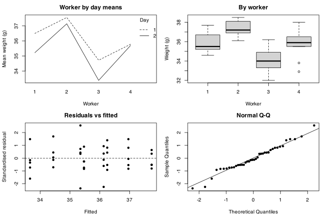
shapiro.test(rstandard(add))
	Shapiro-Wilk normality test

data:  rstandard(add)
W = 0.97626, p-value = 0.5533
The interaction plot shows four near-parallel day-to-day drops, which is the picture behind \(p = 0.51\) for \(H_I\). Residuals are patternless against fitted values and close to Normal (\(p = 0.55\)).
Conclusions.
- Interaction: no evidence (\(F = 0.79\) on \(3, 32\), \(p = 0.51\)). The additive model suffices.
- Workers: strong evidence of differences (\(F = 14.77\) on \(3, 35\), \(p = 2 \times 10^{-6}\)). Relative to worker 1, worker 2 runs \(1.49\) g heavy and worker 3 runs \(1.81\) g light; worker 4 is indistinguishable from worker 1. Tukey intervals show worker 2 differs from workers 1, 3, 4 and worker 3 differs from 1, 2, 4, while workers 1 and 4 do not differ. The spread from worker 3 to worker 2 is \(3.3\) g, or about three residual standard deviations — large enough to matter for a component of “standard size”.
- Days: borderline evidence of a difference (\(F = 4.93\) on \(1, 35\), \(p = 0.033\)). Day 2 components average \(0.78\) g lighter than day 1. This is a real but modest shift, smaller than the worker-to-worker spread, and being significant at only \(p = 0.03\) on a single day-to-day comparison it should not be over-read: two days is far too small a sample to characterise day-to-day process variation.
Practically, the dominant source of variability is the operator, not the day, and worker 3 in particular is producing systematically light components.
Problem 6.7 — For the balanced data in Table 6.12, the analyses in Section 6.4.2 showed
For the balanced data in Table 6.12, the analyses in Section 6.4.2 showed that the hypothesis tests were independent. An alternative specification of the design matrix for the saturated Model (6.9) with the corner point constraints \(\alpha_1 = \beta_1 = (\alpha\beta)_{11} = (\alpha\beta)_{12} = (\alpha\beta)_{21} = (\alpha\beta)_{31} = 0\) is
\begin{equation*} \beta = \begin{bmatrix} \mu \\ \alpha_2 \\ \alpha_3 \\ \beta_2 \\ (\alpha\beta)_{22} \\ (\alpha\beta)_{32} \end{bmatrix}, \qquad X = \begin{bmatrix} 1 & -1 & -1 & -1 & 1 & 1 \\ 1 & -1 & -1 & -1 & 1 & 1 \\ 1 & -1 & -1 & 1 & -1 & -1 \\ 1 & -1 & -1 & 1 & -1 & -1 \\ 1 & 1 & 0 & -1 & -1 & 0 \\ 1 & 1 & 0 & -1 & -1 & 0 \\ 1 & 1 & 0 & 1 & 1 & 0 \\ 1 & 1 & 0 & 1 & 1 & 0 \\ 1 & 0 & 1 & -1 & 0 & -1 \\ 1 & 0 & 1 & -1 & 0 & -1 \\ 1 & 0 & 1 & 1 & 0 & 1 \\ 1 & 0 & 1 & 1 & 0 & 1 \end{bmatrix}, \end{equation*}
where the columns of \(X\) corresponding to the terms \((\alpha\beta)_{jk}\) are the products of columns corresponding to terms \(\alpha_j\) and \(\beta_k\).
a. Show that \(X^T X\) has the block diagonal form described in Section 6.2.5. Fit the Model (6.9) and also Models (6.10) to (6.12) and verify that the results in Table 6.11 are the same for this specification of \(X\).
b. Show that the estimates for the mean of the subgroup with treatments A3 and B2 for two different models are the same as the values given at the end of Section 6.4.2.
Table 6.12 gives, for factor A at three levels and factor B at two levels with two replicates per subgroup: A1B1 \(6.8, 6.6\); A1B2 \(5.3, 6.1\); A2B1 \(7.5, 7.4\); A2B2 \(7.2, 6.5\); A3B1 \(7.8, 9.1\); A3B2 \(8.8, 9.1\). (difficulty: \(\star\star\star\))
A preliminary remark on the wording. The matrix printed is not the corner-point design matrix (which would have \(0/1\) entries); it is an effect-type coding in which the A-columns take values \((-1,-1)\), \((1,0)\), \((0,1)\) on levels A1, A2, A3 and the B-column takes \(-1\) on B1 and \(+1\) on B2. The symbols \(\mu, \alpha_2, \dots\) are re-used as names for the six free parameters, but they no longer mean what they mean under the corner-point constraints. What is preserved is the column space: this \(X\) has rank \(6\) and its columns are constant within each of the six subgroups, so it spans exactly the same six-dimensional space as the corner-point \(X\) of Section 6.4.2. Hence the fitted values, the residual sums of squares and every \(F\) test are unchanged — which is what part (a) asks us to verify. Similarly, the first four columns span the same space as the corner-point additive design (since \(\alpha_2\)-column \(= I_{A2} - I_{A1}\) and \(\alpha_3\)-column \(= I_{A3} - I_{A1}\), together with the constant, span \(\{1, I_{A2}, I_{A3}\}\), and \(\beta_2\)-column \(= 2I_{B2} - 1\)).
A second remark: the cross-reference “Table 6.11” is a misprint. Table 6.11 is the ANOVA table for the plant weight data; the results to be reproduced are those of Table 6.13 (the \(b^T X^T y\) and scaled deviance summary) and Table 6.14 (whose own caption also misprints “Table 6.11” for “Table 6.12”).
Part (a) — block diagonality.
y  <- c(6.8,6.6,5.3,6.1, 7.5,7.4,7.2,6.5, 7.8,9.1,8.8,9.1)
a2 <- rep(c(-1,1,0), each = 4)
a3 <- rep(c(-1,0,1), each = 4)
b2 <- rep(c(-1,-1,1,1), 3)
X  <- cbind(mu = 1, a2 = a2, a3 = a3, b2 = b2, ab22 = a2*b2, ab32 = a3*b2)
t(X) %*% X
     mu a2 a3 b2 ab22 ab32
mu   12  0  0  0    0    0
a2    0  8  4  0    0    0
a3    0  4  8  0    0    0
b2    0  0  0 12    0    0
ab22  0  0  0  0    8    4
ab32  0  0  0  0    4    8
\(X^T X\) is block diagonal with blocks
\begin{equation*} X_1^T X_1 = [12], \quad X_2^T X_2 = \begin{bmatrix} 8 & 4 \\ 4 & 8 \end{bmatrix}, \quad X_3^T X_3 = [12], \quad X_4^T X_4 = \begin{bmatrix} 8 & 4 \\ 4 & 8 \end{bmatrix}, \end{equation*}
corresponding to the partition \(X = [X_1, X_2, X_3, X_4]\) into the constant, the two A-columns, the B-column and the two interaction columns. This is exactly the structure of Section 6.2.5: \(X_j^T X_k = O\) for \(j \neq k\).
The algebra behind the zeros is easy to see. Take \(X_1^T X_2\): the A-columns sum to \(4(-1) + 4(1) + 4(0) = 0\) and \(4(-1) + 4(0) + 4(1) = 0\) over the twelve rows, since each level of A occurs four times. Take \(X_2^T X_3\): within each level of A the B-column takes \(-1\) twice and \(+1\) twice, so the products cancel in pairs. The interaction columns are products \(a_j b_2\), and \(\sum_i a_{ij} b_{i2} \cdot 1 = 0\) and \(\sum_i (a_{ij} b_{i2}) b_{i2} = \sum_i a_{ij} b_{i2}^2 = \sum_i a_{ij} = 0\) for the same reasons. Balance — equal replication in every subgroup — is what makes all this work.
The consequences are those listed in Section 6.2.5: \(b_j = (X_j^T X_j)^{-1} X_j^T y\) does not change when other blocks enter the model, and \(b^T X^T y\) decomposes additively into block contributions.
Xty <- t(X) %*% y
b   <- solve(t(X) %*% X, Xty)
round(data.frame(Xty = Xty[,1], b = b[,1]), 4)
c(yty = sum(y^2), bXty = sum(b * Xty))
      Xty       b
mu   88.2  7.3500
a2    3.8 -0.2000
a3   10.0  1.3500
b2   -2.2 -0.1833
ab22  0.8 -0.1167
ab32  3.0  0.4333
   yty   bXty
664.10 662.62
\(y^T y = 664.10\) and \(b^T X^T y = 662.62\), matching the text exactly, so the saturated model has scaled deviance \(\sigma^2 D_S = 1.48\). Now the nested models: Model (6.10) drops the last two columns, Model (6.11) the last three, Model (6.12) keeps columns 1 and 4.
idx <- list(saturated = 1:6, additive = 1:4, "mu+alpha" = 1:3,
            "mu+beta" = c(1,4), "mu only" = 1)
for (nm in names(idx)) {
  Xi <- X[, idx[[nm]], drop = FALSE]
  bi <- solve(t(Xi) %*% Xi, t(Xi) %*% y)
  cat(sprintf("%-10s df=%2d  bXty=%10.4f  scaled deviance=%8.4f\n",
      nm, 12 - ncol(Xi), sum(bi * (t(Xi) %*% y)),
      sum(y^2) - sum(bi * (t(Xi) %*% y))))
}
saturated  df= 6  bXty=  662.6200  scaled deviance=  1.4800
additive   df= 8  bXty=  661.4133  scaled deviance=  2.6867
mu+alpha   df= 9  bXty=  661.0100  scaled deviance=  3.0900
mu+beta    df=10  bXty=  648.6733  scaled deviance= 15.4267
mu only    df=11  bXty=  648.2700  scaled deviance= 15.8300
Every entry reproduces Table 6.13. Consequently the \(F\) tests are identical: \(F = 2.45\) on \((2,6)\) for \(H_I\), \(F = 1.63\) on \((1,6)\) for \(H_B\), \(F = 25.82\) on \((2,6)\) for \(H_A\).
Finally, the orthogonal partition of Table 6.2 gives Table 6.14 directly, each line computed from its own block alone.
blocks <- list(Mean = 1, "Levels of A" = 2:3, "Levels of B" = 4, "Interactions" = 5:6)
ss <- sapply(blocks, function(j) {
  Xj <- X[, j, drop = FALSE]
  bj <- solve(t(Xj) %*% Xj, t(Xj) %*% y)
  sum(bj * (t(Xj) %*% y))
})
data.frame(df = sapply(blocks, length), SS = round(ss, 4))
c(residual = sum(y^2) - sum(ss), total = sum(y^2))
             df       SS
Mean          1 648.2700
Levels of A   2  12.7400
Levels of B   1   0.4033
Interactions  2   1.2067
residual    total
    1.48   664.10
These are the sums of squares of Table 6.14 — \(648.27\), \(12.74\), \(0.4033\), \(1.2067\), residual \(1.48\), total \(664.10\) — and they were obtained without ever fitting the other terms. That is the concrete content of “the hypothesis tests are independent”: with an orthogonal \(X\), each block’s contribution is a fixed number, so it does not matter in which order terms are entered.
Part (b) — the A3, B2 subgroup mean.
The A3B2 rows of \(X\) (rows 11 and 12) are \((1, 0, 1, 1, 0, 1)\), so the saturated-model estimate of that subgroup mean is \(\hat\mu + \hat\alpha_3 + \hat\beta_2 + \widehat{(\alpha\beta)}_{32}\); for the additive model it is the first four entries only.
badd <- solve(t(X[,1:4]) %*% X[,1:4], t(X[,1:4]) %*% y)
round(t(badd), 4)
c(saturated = sum(X[11, ] * b), additive = sum(X[11, 1:4] * badd))
       mu   a2   a3      b2
[1,] 7.35 -0.2 1.35 -0.1833
saturated  additive
 8.950000  8.516667
The saturated model gives \(7.35 + 1.35 - 0.1833 + 0.4333 = 8.95\) and the additive model gives \(7.35 + 1.35 - 0.1833 = 8.5167\). These are precisely the values \(8.95\) and \(8.516\) quoted at the end of Section 6.4.2, even though the parameter estimates themselves are different numbers from the corner-point ones (\(6.7, 1.75, -1.0, 1.5\) there). That has to be so: fitted values depend on the column space, not on the parametrisation of it.
Notice also the orthogonality at work in the estimates: \(\hat\mu, \hat\alpha_2, \hat\alpha_3, \hat\beta_2\) take the same values \(7.35, -0.20, 1.35, -0.1833\) in the additive model as in the saturated one. Dropping the interaction block leaves the other blocks’ estimates untouched, exactly as Section 6.2.5 predicts. And the gap between \(8.95\) and \(8.52\) is the point the text makes: which model you choose changes the summary you report for a subgroup, even when the model comparison (\(F = 2.45\), not significant) gives no strong reason to prefer the larger one.
Problem 6.8 — Table 6.27 shows the data from a fictitious two-factor experiment.
Table 6.27 shows the data from a fictitious two-factor experiment.
a. Test the hypothesis that there are no interaction effects.
b. Test the hypothesis that there is no effect due to Factor A (i) by comparing the models \[ E(Y_{jkl}) = \mu + \alpha_j + \beta_k \quad \text{and} \quad E(Y_{jkl}) = \mu + \beta_k; \] (ii) by comparing the models \[ E(Y_{jkl}) = \mu + \alpha_j \quad \text{and} \quad E(Y_{jkl}) = \mu. \]
Explain the results.
Table 6.27 Two-factor experiment with unbalanced data. Factor A has three levels and factor B two. Cell A1B1 contains the single value \(5\); A1B2 contains \(3, 4\); A2B1 contains \(6, 4\); A2B2 contains \(4, 3\); A3B1 contains \(7\); A3B2 contains \(6, 8\). (difficulty: \(\star\star\))
This is the counterpart of Exercise 6.7: there the data were balanced and the tests were independent, here the subgroup sizes are \(1, 2, 2, 2, 1, 2\) and they are not. The models are (6.9) to (6.12) again, with \(N = 10\).
library(dobson)
data(unbalanced)
ub <- as.data.frame(unbalanced)
ub$factorA <- factor(ub$factorA); ub$factorB <- factor(ub$factorB)
table(ub$factorA, ub$factorB)
tapply(ub$data, list(ub$factorA, ub$factorB), mean)
     B1 B2
  A1  1  2
  A2  2  2
  A3  1  2
   B1  B2
A1  5 3.5
A2  5 3.5
A3  7 7.0
sat <- lm(data ~ factorA * factorB, data = ub)   # Model (6.9)
add <- lm(data ~ factorA + factorB, data = ub)   # Model (6.10)
mA  <- lm(data ~ factorA, data = ub)             # Model (6.11)
mB  <- lm(data ~ factorB, data = ub)             # Model (6.12)
m0  <- lm(data ~ 1, data = ub)
round(t(sapply(list(saturated = sat, additive = add, A_only = mA,
                    B_only = mB, mean = m0),
               function(m) c(df = df.residual(m), RSS = deviance(m)))), 4)
          df     RSS
saturated  4  5.0000
additive   6  6.0714
A_only     7  8.7500
B_only     8 24.3333
mean       9 26.0000
Part (a) — no interaction.
anova(add, sat)
Analysis of Variance Table

Model 1: data ~ factorA + factorB
Model 2: data ~ factorA * factorB
  Res.Df    RSS Df Sum of Sq      F Pr(>F)
1      6 6.0714
2      4 5.0000  2    1.0714 0.4286 0.6782
\(F = (1.0714/2)/(5.0000/4) = 0.43\) on \(2\) and \(4\) degrees of freedom, \(p = 0.68\). There is no evidence against \(H_I\). (Looking at the cell means, the B1 minus B2 difference is \(1.5\) at levels A1 and A2 but \(0\) at A3 — a hint of interaction, but with only four residual degrees of freedom the test cannot resolve it.) Having failed to reject \(H_I\) we go on to test the main effect of A.
Part (b)(i) — A adjusted for B.
anova(mB, add)
Analysis of Variance Table

Model 1: data ~ factorB
Model 2: data ~ factorA + factorB
  Res.Df     RSS Df Sum of Sq      F  Pr(>F)
1      8 24.3333
2      6  6.0714  2    18.262 9.0235 0.01553 *
---
Signif. codes:  0 ‘***’ 0.001 ‘**’ 0.01 ‘*’ 0.05 ‘.’ 0.1 ‘ ’ 1
Improvement \(24.3333 - 6.0714 = 18.262\) on \(2\) d.f., residual mean square \(6.0714/6 = 1.0119\), so
\begin{equation*} F = \frac{18.262/2}{6.0714/6} = 9.02 \sim F(2,6), \qquad p = 0.016. \end{equation*}
Part (b)(ii) — A alone.
anova(m0, mA)
Analysis of Variance Table

Model 1: data ~ 1
Model 2: data ~ factorA
  Res.Df   RSS Df Sum of Sq   F  Pr(>F)
1      9 26.00
2      7  8.75  2     17.25 6.9 0.02211 *
---
Signif. codes:  0 ‘***’ 0.001 ‘**’ 0.01 ‘*’ 0.05 ‘.’ 0.1 ‘ ’ 1
Improvement \(26.00 - 8.75 = 17.25\) on \(2\) d.f., residual mean square \(8.75/7 = 1.25\), so \(F = 8.625/1.25 = 6.90\) on \(2\) and \(7\) degrees of freedom, \(p = 0.022\).
Explaining the results.
The two tests of “no effect due to factor A” give different sums of squares — \(18.262\) with B in the model, \(17.250\) without — and different \(F\) statistics, \(9.02\) versus \(6.90\). In Exercise 6.7, with balanced data, the corresponding pair of tests gave the identical sum of squares \(0.4033\) twice over. The difference is orthogonality.
With unequal subgroup sizes the design matrix cannot be partitioned into orthogonal blocks: the columns for factor A are not orthogonal to the column for factor B, because level A1 is observed once at B1 and twice at B2 while A2 is observed twice at each. Consequently \(X^T X\) is not block diagonal, \(b^T X^T y\) does not split additively into a part for A and a part for B, and the sum of squares “for A” depends on whether B has already been fitted. This is precisely the Type I versus Type III distinction noted at the end of Section 6.2.5.
Two further points are worth separating out.
- The numerators differ because of non-orthogonality, as just described. Test (i) measures how much A explains after B has taken what it can; test (ii) measures how much A explains on its own, and part of what A explains on its own is really B acting through the unequal cell counts.
- The denominators differ too, and for a more mundane reason: test (ii) uses \(\hat\sigma^2\) from a model that omits B, so any real B effect is left in the residual and inflates the error estimate (\(1.25\) versus \(1.0119\)). This alone pushes \(F\) down.
Here both tests happen to reach the same verdict — reject \(H_A\) at the \(5\%\) level — so the conclusion is robust: factor A does affect the response. The fitted additive model puts A3 about \(3.0\) units above A1 (\(t = 3.65\), \(p = 0.011\)) while A2 is indistinguishable from A1 (\(0.07\) units), and the B effect is a non-significant \(-1.07\) (\(p = 0.15\)). But the reported sums of squares and \(p\)-values depend on the order of fitting, and with a less clear-cut data set the two routes could easily land on opposite sides of \(0.05\). The practical rule is to state which terms were already in the model whenever an unbalanced ANOVA sum of squares is quoted.
Problem 6.9 — Examine if there is a non-linear association between age and cholesterol
Examine if there is a non-linear association between age and cholesterol using the fractional polynomial approach for the data in Table 6.24 (serum cholesterol, age and body mass index for thirty women, transcribed in Exercise 6.4). (difficulty: \(\star\star\))
The fractional polynomial approach of Section 6.8 fits
\begin{equation*} E(Y_i) = \beta_0 + \beta_1 x_i^p, \qquad i = 1, \dots, N, \end{equation*}
for the eight candidate powers \(p \in \{-2, -1, -0.5, 0, 0.5, 1, 2, 3\}\), where \(x^0\) means \(\log_e x\). Every one of these models has the same two parameters, so they can be ranked directly on residual sum of squares — no penalty term is needed, which is what makes the method convenient. Following the text’s advice we scale \(x\) first; ages here run from \(21\) to \(78\), so \(x = \text{age}/50\) puts the covariate near \(1\) and keeps the powers numerically comparable.
library(dobson)
data(cholesterol)
ch <- as.data.frame(cholesterol)
x  <- ch$age / 50
y  <- ch$chol
tf <- function(x, p) if (p == 0) log(x) else x^p
ps <- c(-2, -1, -0.5, 0, 0.5, 1, 2, 3)
res <- t(sapply(ps, function(p) {
  m <- lm(y ~ tf(x, p))
  c(p = p, RSS = deviance(m), AIC = AIC(m), R2 = summary(m)$r.squared)
}))
round(res, 4)
        p     RSS     AIC     R2
[1,] -2.0 39.8864 99.6815 0.1975
[2,] -1.0 36.2897 96.8464 0.2699
[3,] -0.5 34.6522 95.4613 0.3028
[4,]  0.0 33.2927 94.2605 0.3302
[5,]  0.5 32.2819 93.3356 0.3505
[6,]  1.0 31.6362 92.7294 0.3635
[7,]  2.0 31.3148 92.4231 0.3700
[8,]  3.0 31.9312 93.0079 0.3576
The profile is smooth and shallow, with a minimum at \(p = 2\) (RSS \(31.315\)) and the straight line \(p = 1\) essentially tied behind it (RSS \(31.636\)).
par(mfrow = c(1,2), mar = c(4.5,4.5,3,1))
plot(res[,"p"], res[,"RSS"], type = "b", pch = 16, xlab = "Power p",
     ylab = "Residual sum of squares", main = "Fractional polynomial profile")
abline(h = min(res[,"RSS"]), lty = 3)
plot(ch$age, y, pch = 16, xlab = "Age (years)",
     ylab = "Serum cholesterol (mmol/l)", main = "Fitted curves")
g <- seq(min(ch$age), max(ch$age), length = 200); gs <- g / 50
for (p in c(1, 2, -1)) {
  m <- lm(y ~ tf(x, p)); k <- which(c(1,2,-1) == p)
  lines(g, coef(m)[1] + coef(m)[2]*tf(gs, p), lty = k,
        col = c("black","red","blue")[k])
}
legend("topleft", c("p = 1 (linear)","p = 2 (best)","p = -1"),
       lty = 1:3, col = c("black","red","blue"), bty = "n")
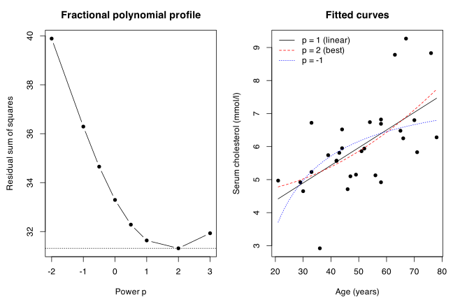
summary(lm(y ~ tf(x, 2)))
Call:
lm(formula = y ~ tf(x, 2))

Residuals:
     Min       1Q   Median       3Q      Max
-2.30772 -0.59886  0.03643  0.39275  2.37140

Coefficients:
            Estimate Std. Error t value Pr(>|t|)
(Intercept)   4.5495     0.4076  11.162 8.05e-12 ***
tf(x, 2)      1.3082     0.3226   4.055 0.000363 ***
---
Signif. codes:  0 ‘***’ 0.001 ‘**’ 0.01 ‘*’ 0.05 ‘.’ 0.1 ‘ ’ 1

Residual standard error: 1.058 on 28 degrees of freedom
Multiple R-squared:   0.37,	Adjusted R-squared:  0.3475
F-statistic: 16.44 on 1 and 28 DF,  p-value: 0.0003627
Is the non-linearity real? The gain from \(p = 1\) to \(p = 2\) is \(31.636 - 31.315 = 0.32\) out of a total sum of squares of \(49.7\) — about \(0.6\%\) of the residual variation, and \(R^2\) moves from \(0.364\) to \(0.370\). The fitted-curve panel shows why: through the bulk of the age range the \(p = 2\) curve and the straight line are almost indistinguishable, separating only at the extremes, where the data are thinnest.
The eight-way comparison is a selection exercise, not a test, so it cannot by itself say whether the curvature is more than noise. A test is available by embedding both in one model: the quadratic \(E(Y) = \beta_0 + \beta_1 x + \beta_2 x^2\) contains the straight line as \(\beta_2 = 0\).
anova(lm(y ~ x), lm(y ~ x + I(x^2)))
Analysis of Variance Table

Model 1: y ~ x
Model 2: y ~ x + I(x^2)
  Res.Df    RSS Df Sum of Sq      F Pr(>F)
1     28 31.636
2     27 31.307  1   0.32941 0.2841 0.5984
\(F = 0.28\) on \(1\) and \(27\) degrees of freedom, \(p = 0.60\): no evidence of curvature. The same holds after adjusting for body mass index, the covariate found relevant in Exercise 6.4.
anova(lm(chol ~ age + bmi, data = ch), lm(chol ~ age + I(age^2) + bmi, data = ch))
Analysis of Variance Table

Model 1: chol ~ age + bmi
Model 2: chol ~ age + I(age^2) + bmi
  Res.Df    RSS Df Sum of Sq      F Pr(>F)
1     27 26.571
2     26 25.992  1   0.57809 0.5783 0.4538
Conclusion. The fractional polynomial search nominates \(p = 2\), but the improvement over the linear fit is negligible and a formal test finds no curvature (\(p = 0.60\) unadjusted, \(p = 0.45\) adjusted for BMI). With \(N = 30\) observations spread over ages \(21\) to \(78\) these data give no evidence of a non-linear association between age and cholesterol; the simple linear term of Exercise 6.4 — \(0.053\) mmol/l per year of age — remains the appropriate summary.
Two cautions on method, since the exercise is really about the technique. First, the ranking is shallow: the RSS profile is nearly flat between \(p = 0.5\) and \(p = 3\), so which power “wins” is decided by differences well inside sampling noise, and a slightly different sample would nominate a different \(p\). Contrast this with the PLOS Medicine example of Section 6.8, where the winner (\(p = -0.5\), RSS \(846{,}761\)) beat the linear fit (\(943{,}484\)) by more than \(10\%\) — there the choice meant something. Second, the standard errors and \(p\)-values reported for the selected model take no account of the fact that \(p\) was chosen from the same data; they are optimistic, which is a further reason not to read the \(p = 2\) selection as a finding.
Binary Variables and Logistic Regression
Problem 7.1 — The number of deaths from leukemia and other cancers among survivors
The number of deaths from leukemia and other cancers among survivors of the Hiroshima atom bomb are shown in Table 7.14, classified by the radiation dose received. The data refer to deaths during the period 1950–1959 among survivors who were aged 25 to 64 years in 1950 (from data set 13 of Cox and Snell, 1981, attributed to Otake, 1979).
a. Obtain a suitable model to describe the dose–response association between radiation and the proportional cancer mortality rates for leukemia. b. Examine how well the model describes the data. c. Interpret the results.
Table 7.14 (deaths from leukemia and other cancers classified by radiation dose received from the Hiroshima atomic bomb) has one column per radiation dose band, in rads: \(0\), \(1\)–\(9\), \(10\)–\(49\), \(50\)–\(99\), \(100\)–\(199\), \(200+\). The rows are
- Leukemia deaths
- 13, 5, 5, 3, 4, 18
- Other cancer deaths
- 378, 200, 151, 47, 31, 33
- Total cancer deaths
- 391, 205, 156, 50, 35, 51
(difficulty: \(\star\star\))
Setting up. A proportional mortality rate is the share of all cancer deaths that are leukemia deaths, so the response for dose band \(i\) is \[ Y_i \sim \text{Bin}(n_i, \pi_i), \qquad n_i = \text{total cancer deaths}, \qquad \pi_i = \Pr(\text{death is leukemia} \mid \text{cancer death}). \] This is the setting of Section 7.4: a Binomial response with \(N = 6\) covariate patterns. Note what the denominators buy us – the number of survivors at each dose is unknown, but conditioning on “died of cancer” removes it, at the price of interpreting the results as leukemia deaths relative to other cancer deaths rather than as absolute risks.
The dose bands are intervals, so a numeric dose \(x_i\) must be assigned. I use the band midpoints \(0\), \(5\), \(29.5\), \(74.5\), \(149.5\) rads and, for the open-ended \(200+\) band, \(300\) rads. The last value is a judgement call and I check its influence below.
library(dobson)
data(hiroshima)
h <- hiroshima
names(h) <- c("dose", "leuk", "other", "total")
h$mid <- c(0, 5, 29.5, 74.5, 149.5, 300)
h$p <- h$leuk / h$total
data.frame(dose = as.character(h$dose), n = h$total, y = h$leuk,
mid = h$mid, p = round(h$p, 4),
logit = round(log(h$p / (1 - h$p)), 3))
dose n y mid p logit
1 0 391 13 0.0 0.0332 -3.370
2 1 to 9 205 5 5.0 0.0244 -3.689
3 10 to 49 156 5 29.5 0.0321 -3.408
4 50 to 99 50 3 74.5 0.0600 -2.752
5 100 to 199 35 4 149.5 0.1143 -2.048
6 200 + 51 18 300.0 0.3529 -0.606
The empirical logits are close to linear in dose, which is what the logistic dose–response model of Section 7.3 assumes.
(a) The model. Fit \[ \log\left(\frac{\pi_i}{1-\pi_i}\right) = \beta_1 + \beta_2 x_i, \] by maximum likelihood, i.e. maximising the log-likelihood (7.4).
m1 <- glm(cbind(leuk, other) ~ mid, family = binomial, data = h)
summary(m1)
Call:
glm(formula = cbind(leuk, other) ~ mid, family = binomial, data = h)
Coefficients:
Estimate Std. Error z value Pr(>|z|)
(Intercept) -3.523825 0.206908 -17.031 < 2e-16 ***
mid 0.009716 0.001228 7.912 2.53e-15 ***
---
Signif. codes: 0 '***' 0.001 '**' 0.01 '*' 0.05 '.' 0.1 ' ' 1
(Dispersion parameter for binomial family taken to be 1)
Null deviance: 54.35089 on 5 degrees of freedom
Residual deviance: 0.67956 on 4 degrees of freedom
AIC: 26.345
Number of Fisher Scoring iterations: 4
So \(b_1 = -3.524\ (0.207)\) and \(b_2 = 0.009716\ (0.001228)\).
The dose effect is overwhelming: the drop in deviance from the minimal model to this one is \(C = 54.351 - 0.680 = 53.67\) on \(1\) degree of freedom, which is the likelihood ratio chi-squared statistic of Section 7.5 (and Exercise 7.4), far beyond any tabulated \(\chi^2(1)\) value.
(b) How well the model describes the data. The residual deviance (7.5) is \(D = 0.680\) on \(N - p = 6 - 2 = 4\) degrees of freedom, and the Pearson statistic (7.6) is \(X^2 = 0.672\), also on \(4\) degrees of freedom.
X2 <- sum(residuals(m1, type = "pearson")^2)
c(deviance = deviance(m1), pearson = X2, df = df.residual(m1),
p_dev = pchisq(deviance(m1), 4, lower.tail = FALSE),
p_X2 = pchisq(X2, 4, lower.tail = FALSE))
deviance pearson df p_dev p_X2
0.6795634 0.6716142 4.0000000 0.9538250 0.9547828
Both are far below their expected value of 4, with \(p \approx 0.95\); the fit is if anything suspiciously good, which is common when a smooth monotone trend runs through only six points. Cell-by-cell, no fitted count is small (the smallest expected leukemia count is 2.9, above the “less than 1” threshold flagged in Section 7.5) and no residual is remotely large.
data.frame(dose = as.character(h$dose), obs = h$leuk,
fitted = round(fitted(m1) * h$total, 2),
pearson = round(residuals(m1, "pearson"), 3),
deviance = round(residuals(m1, "deviance"), 3))
dose obs fitted pearson deviance
1 0 13 11.20 0.546 0.533
2 1 to 9 5 6.16 -0.473 -0.488
3 10 to 49 5 5.90 -0.376 -0.386
4 50 to 99 3 2.87 0.081 0.081
5 100 to 199 4 3.92 0.044 0.044
6 200 + 18 17.97 0.010 0.010
Three further checks. Adding a quadratic in dose buys nothing; the saturated (dose as a factor) model has a worse AIC than the two-parameter linear model; and the probit and complementary log-log links of Section 7.3 fit no better than the logit, so the data cannot discriminate between links here – which is expected, since all the fitted probabilities are below \(0.4\) where the three links are close.
mq <- glm(cbind(leuk, other) ~ mid + I(mid^2), family = binomial, data = h)
mf <- glm(cbind(leuk, other) ~ factor(dose), family = binomial, data = h)
c(dev_quad = deviance(mq), p_quadratic_term = summary(mq)$coef[3, 4],
AIC_linear = AIC(m1), AIC_saturated = AIC(mf),
dev_probit = deviance(glm(cbind(leuk, other) ~ mid, binomial("probit"), data = h)),
dev_cloglog = deviance(glm(cbind(leuk, other) ~ mid, binomial("cloglog"), data = h)))
dev_quad p_quadratic_term AIC_linear AIC_saturated
0.6687957 0.9176481 26.3445651 33.6650017
dev_probit dev_cloglog
0.8440787 0.6791914
The one genuinely soft assumption is the score of \(300\) rads for the open-ended top band. Refitting with \(250\) and \(400\) moves the slope but not the conclusion:
sapply(c(250, 300, 400), function(top) {
h$mid <- c(0, 5, 29.5, 74.5, 149.5, top)
m <- glm(cbind(leuk, other) ~ mid, family = binomial, data = h)
c(slope = coef(m)[2], deviance = deviance(m))
})
[,1] [,2] [,3]
slope.mid 0.01160255 0.009716222 0.007232667
deviance 1.02076456 0.679563424 1.055412491
The slope is inversely proportional to the assumed midpoint, as it must be, and the fit is good under all three. So the shape of the dose–response relation is well established; the numerical value of “risk per rad” is only as good as the dose scoring.
The fitted curve against the data, on both the probability and the logit scale:
par(mfrow = c(1, 2), mar = c(4.5, 4.5, 2, 1))
plot(h$mid, h$p, pch = 19, ylim = c(0, 0.45), main = "Proportion scale",
xlab = "Radiation dose (rads, group midpoint)",
ylab = "Proportion of cancer deaths that are leukemia")
xx <- seq(0, 320, length = 200)
lines(xx, predict(m1, newdata = data.frame(mid = xx), type = "response"), lwd = 2)
plot(h$mid, log(h$p / (1 - h$p)), pch = 19, main = "Logit scale",
xlab = "Radiation dose (rads, group midpoint)", ylab = "Empirical logit")
abline(coef(m1), lwd = 2)
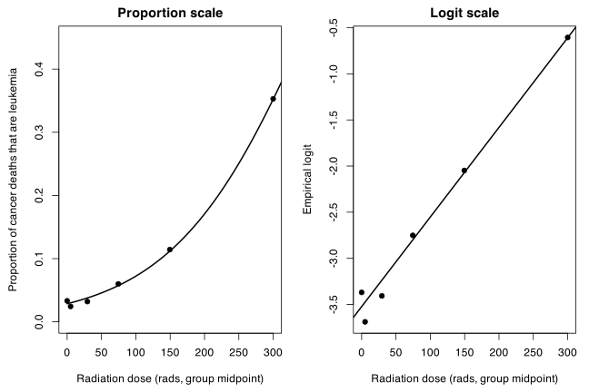
(c) Interpretation. The estimated log-odds of a cancer death being a leukemia death rises linearly with dose at \(0.00972\) per rad. Exponentiating, each extra \(100\) rads multiplies the odds by \[ \exp(100 \times 0.009716) = 2.64, \] with a Wald 95% interval \(\exp(100 \times (0.009716 \pm 1.96 \times 0.001228)) = (2.08,\ 3.36)\).
exp(100 * c(est = coef(m1)[2], confint.default(m1)[2, ]))
est.mid 2.5 % 97.5 %
2.642227 2.077027 3.361230
At zero dose the model gives \(\hat{\pi} = e^{-3.524}/(1 + e^{-3.524}) = 0.0286\), i.e. about 3% of cancer deaths are leukemia deaths – the background proportion. At \(300\) rads the fitted proportion is \(0.352\), a twelve-fold increase in the share. In words: radiation raises the leukemia death rate much more steeply than it raises the death rate from other cancers, and the excess is dose-dependent over the whole observed range with no sign of a threshold below which the effect vanishes.
Two cautions on the reading. First, because the denominator is total cancer deaths, the estimate is a relative statement – it is consistent with radiation raising both leukemia and other cancers, provided it raises leukemia faster. Second, the warning of Section 7.9 applies: an odds ratio of \(2.64\) per \(100\) rads is not a “2.64 times more likely” statement about risk. Since the baseline proportion is small, the two happen to be close at low dose (the fitted proportion ratio from \(0\) to \(100\) rads is \(0.0723/0.0286 = 2.53\)), but by \(200\)–\(300\) rads the odds ratio badly overstates the proportion ratio.
Problem 7.2 — Odds ratios. Consider a 2×2 contingency table from a prospective study
Odds ratios. Consider a \(2 \times 2\) contingency table from a prospective study in which people who were or were not exposed to some pollutant are followed up and, after several years, categorized according to the presence or absence of a disease. Table 7.15 shows the probabilities for each cell: the row “Exposed” has probability \(\pi_1\) of being diseased and \(1 - \pi_1\) of not being diseased, and the row “Not exposed” has probability \(\pi_2\) of being diseased and \(1 - \pi_2\) of not being diseased. The odds of disease for either exposure group is \(O_i = \pi_i/(1 - \pi_i)\), for \(i = 1, 2\), and so the odds ratio \[ \phi = \frac{O_1}{O_2} = \frac{\pi_1(1 - \pi_2)}{\pi_2(1 - \pi_1)} \] is a measure of the relative likelihood of disease for the exposed and not exposed groups.
a. For the simple logistic model \(\pi_i = e^{\beta_i}/(1 + e^{\beta_i})\), show that if there is no difference between the exposed and not exposed groups (i.e., \(\beta_1 = \beta_2\)), then \(\phi = 1\). b. Consider \(J\) \(2 \times 2\) tables like Table 7.15, one for each level \(x_j\) of a factor, such as age group, with \(j = 1, \ldots, J\). For the logistic model \[ \pi_{ij} = \frac{\exp(\alpha_i + \beta_i x_j)}{1 + \exp(\alpha_i + \beta_i x_j)}, \qquad i = 1, 2, \quad j = 1, \ldots, J. \] Show that \(\log \phi\) is constant over all tables if \(\beta_1 = \beta_2\) (McKinlay 1978).
(difficulty: \(\star\))
This is pure algebra; the point of the exercise is that the logit link turns odds ratios into differences of linear predictors, which is the fact quoted in Section 7.9 when the chapter warns against reading odds ratios as prevalence ratios.
(a) Under \(\pi_i = e^{\beta_i}/(1 + e^{\beta_i})\) we have \(1 - \pi_i = 1/(1 + e^{\beta_i})\), so the odds are \[ O_i = \frac{\pi_i}{1 - \pi_i} = \frac{e^{\beta_i}/(1 + e^{\beta_i})}{1/(1 + e^{\beta_i})} = e^{\beta_i}. \] This is just the statement that the model is \(\text{logit}\,\pi_i = \beta_i\). Hence \[ \phi = \frac{O_1}{O_2} = \frac{e^{\beta_1}}{e^{\beta_2}} = e^{\beta_1 - \beta_2}, \qquad \text{so} \qquad \log \phi = \beta_1 - \beta_2. \] If \(\beta_1 = \beta_2\) then \(\log \phi = 0\) and \(\phi = e^0 = 1\). The converse also holds: \(\phi = 1\) forces \(\beta_1 = \beta_2\), so “no exposure effect” and “unit odds ratio” are the same hypothesis in this parameterization.
(b) Fix the level \(x_j\) of the stratifying factor. Exactly as in part (a), the model \(\text{logit}\,\pi_{ij} = \alpha_i + \beta_i x_j\) gives the odds within the \(j\)-th table as \[ O_{ij} = \frac{\pi_{ij}}{1 - \pi_{ij}} = \exp(\alpha_i + \beta_i x_j), \qquad i = 1, 2. \] The odds ratio for the \(j\)-th table is therefore \[ \phi_j = \frac{O_{1j}}{O_{2j}} = \frac{\exp(\alpha_1 + \beta_1 x_j)}{\exp(\alpha_2 + \beta_2 x_j)} = \exp\left[(\alpha_1 - \alpha_2) + (\beta_1 - \beta_2)x_j\right], \] so that \[ \log \phi_j = (\alpha_1 - \alpha_2) + (\beta_1 - \beta_2)x_j. \qquad (\ast) \] The only \(j\)-dependence in \((\ast)\) is through the term \((\beta_1 - \beta_2)x_j\). If \(\beta_1 = \beta_2\) this term vanishes and \[ \log \phi_j = \alpha_1 - \alpha_2 \quad \text{for every } j, \] i.e. \(\log \phi\) is the same constant in all \(J\) tables, and the common odds ratio is \(\phi = \exp(\alpha_1 - \alpha_2)\).
Conversely, provided the \(x_j\) are not all equal, \((\ast)\) is constant in \(j\) only if \(\beta_1 - \beta_2 = 0\). So “equal slopes” and “homogeneous odds ratio across strata” are the same assumption – the no-interaction hypothesis. In the language of Section 7.4 this is the difference between Model 1 (different intercepts and slopes) and Model 2 (different intercepts, common slope) fitted to the anther data: Model 2 asserts one odds ratio for treatment versus control that holds at every centrifuging force, which is why Table 7.6 reports \(a_2 - a_1 = 0.407\) as a single number and Section 7.9 converts it to the single odds ratio \(\exp(0.407) = 1.502\).
Two remarks worth making. First, \((\ast)\) shows the interaction is linear in \(x_j\) under this model: unequal slopes do not merely make \(\log \phi_j\) vary, they make it vary linearly in the stratum score. Second, none of this requires the design to be prospective for the algebra to work, but the interpretation of \(\pi_i\) as a disease risk does; in a case-control study the intercepts \(\alpha_i\) absorb the sampling fractions and only the odds ratio remains estimable, which is the usual argument for reporting \(\phi\) rather than a risk difference.
The algebra is easy to slip, so here is a numerical check rather than a derivation: with \(\alpha_1 = -3.0\), \(\alpha_2 = -3.8\) and a common slope \(\beta = 0.04\) over five age levels, \(\log \phi_j\) should equal \(\alpha_1 - \alpha_2 = 0.8\) in every stratum.
x <- c(25, 35, 45, 55, 65)
a <- c(-3.0, -3.8)
b <- c(0.04, 0.04)
pi <- outer(1:2, x, function(i, xj) plogis(a[i] + b[i] * xj))
odds <- pi / (1 - pi)
round(rbind(pi1 = pi[1, ], pi2 = pi[2, ], logphi = log(odds[1, ] / odds[2, ])), 4)
[,1] [,2] [,3] [,4] [,5]
pi1 0.1192 0.1680 0.2315 0.310 0.4013
pi2 0.0573 0.0832 0.1192 0.168 0.2315
logphi 0.8000 0.8000 0.8000 0.800 0.8000
Note that the risks \(\pi_{1j}, \pi_{2j}\) change a great deal across strata while \(\log \phi_j\) does not – that stability is exactly what the constant-odds-ratio model buys. With unequal slopes (\(\beta_1 = 0.04\), \(\beta_2 = 0.06\)) the log odds ratio instead runs down linearly in \(x_j\) with slope \(\beta_1 - \beta_2 = -0.02\):
b2 <- c(0.04, 0.06)
pi <- outer(1:2, x, function(i, xj) plogis(a[i] + b2[i] * xj))
odds <- pi / (1 - pi)
round(log(odds[1, ] / odds[2, ]), 4)
[1] 0.3 0.1 -0.1 -0.3 -0.5
Problem 7.3 — Tables 7.16 and 7.17 show the survival 50 years after graduation of men
Tables 7.16 and 7.17 show the survival 50 years after graduation of men and women who graduated each year from 1938 to 1947 from various faculties of the University of Adelaide (data compiled by J.A. Keats). The columns labelled \(S\) contain the number of graduates who survived and the columns labelled \(T\) contain the total number of graduates. There were insufficient women graduates from the faculties of Medicine and Engineering to warrant analysis.
a. Are the proportions of graduates who survived for 50 years after graduation the same all years of graduation? b. Are the proportions of male graduates who survived for 50 years after graduation the same for all Faculties? c. Are the proportions of female graduates who survived for 50 years after graduation the same for Arts and Science? d. Is the difference between men and women in the proportion of graduates who survived for 50 years after graduation the same for Arts and Science?
Table 7.16 (men) gives \(S\) and \(T\) by year of graduation for four faculties. Medicine: 1938 (18, 22), 1939 (16, 23), 1940 (7, 17), 1941 (12, 25), 1942 (24, 50), 1943 (16, 21), 1944 (22, 32), 1945 (12, 14), 1946 (22, 34), 1947 (28, 37); total (177, 275). Arts: 1938 (16, 30), 1939 (13, 22), 1940 (11, 25), 1941 (12, 14), 1942 (8, 12), 1943 (11, 20), 1944 (4, 10), 1945 (4, 12), 1946 no entry, 1947 (13, 23); total (92, 168). Science: 1938 (9, 14), 1939 (9, 12), 1940 (12, 19), 1941 (12, 15), 1942 (20, 28), 1943 (16, 21), 1944 (25, 31), 1945 (32, 38), 1946 (4, 5), 1947 (25, 31); total (164, 214). Engineering: 1938 (10, 16), 1939 (7, 11), 1940 (12, 15), 1941 (8, 9), 1942 (5, 7), 1943 (1, 2), 1944 (16, 22), 1945 (19, 25), 1946 no entry, 1947 (25, 35); total as printed (100, 139).
Table 7.17 (women) gives \(S\) and \(T\) for two faculties. Arts: 1938 (14, 19), 1939 (11, 16), 1940 (15, 18), 1941 (15, 21), 1942 (8, 9), 1943 (13, 13), 1944 (18, 22), 1945 (18, 22), 1946 (1, 1), 1947 (13, 16); total (126, 157). Science: 1938 (1, 1), 1939 (4, 4), 1940 (6, 7), 1941 (3, 3), 1942 (4, 4), 1943 (8, 9), 1944 (5, 5), 1945 (16, 17), 1946 (1, 1), 1947 (10, 10); total (58, 61).
(difficulty: \(\star\star\))
Setting up. Each cell is a Binomial count: \(S_{fsy} \sim \text{Bin}(T_{fsy}, \pi_{fsy})\) for faculty \(f\), sex \(s\), year \(y\). All four questions are comparisons of nested logistic models, tested by differences of deviance (7.5) as in Section 7.5, so the whole exercise is one analysis-of-deviance table read four ways.
library(dobson)
data(graduates)
g <- subset(as.data.frame(graduates), survive != "*")
g$survive <- as.numeric(g$survive)
g$total <- as.numeric(g$total)
g$died <- g$total - g$survive
g$faculty <- factor(g$faculty)
g$sex <- factor(g$sex)
tab <- aggregate(cbind(survive, total) ~ faculty + sex, data = g, FUN = sum)
tab$p <- round(tab$survive / tab$total, 3)
tab
faculty sex survive total p
1 arts men 92 168 0.548
2 engineering men 103 142 0.725
3 medicine men 177 275 0.644
4 science men 164 214 0.766
5 arts women 126 157 0.803
6 science women 58 61 0.951
The two cells with no graduates (Arts men and Engineering men in 1946) are stored as * in the package and dropped. One data note: the Engineering column totals recomputed from its entries are \(S = 103\), \(T = 142\), whereas Table 7.16 prints \(100\) and \(139\); the printed totals are three short. I work from the yearly entries, which are what the models use.
Even before modelling the pattern is clear – women survive better than men, Science better than Arts.
(a) Year of graduation. Test whether \(\pi\) depends on year, after allowing for faculty and sex (the groups are not balanced across years, so year must be tested adjusted). Fit year both as a \(9\)-degree-of-freedom factor and as a linear trend.
base <- glm(cbind(survive, died) ~ faculty * sex, family = binomial, data = g)
yr_f <- glm(cbind(survive, died) ~ faculty * sex + factor(year), family = binomial, data = g)
anova(base, yr_f, test = "Chisq")
Analysis of Deviance Table
Model 1: cbind(survive, died) ~ faculty * sex
Model 2: cbind(survive, died) ~ faculty * sex + factor(year)
Resid. Df Resid. Dev Df Deviance Pr(>Chi)
1 52 56.765
2 43 47.694 9 9.071 0.4307
yr_l <- glm(cbind(survive, died) ~ faculty * sex + I(year - 1938), family = binomial, data = g)
anova(base, yr_l, test = "Chisq")
Analysis of Deviance Table
Model 1: cbind(survive, died) ~ faculty * sex
Model 2: cbind(survive, died) ~ faculty * sex + I(year - 1938)
Resid. Df Resid. Dev Df Deviance Pr(>Chi)
1 52 56.765
2 51 53.314 1 3.4505 0.06323 .
---
Signif. codes: 0 '***' 0.001 '**' 0.01 '*' 0.05 '.' 0.1 ' ' 1
The unstructured year effect gives \(\Delta D = 9.07\) on \(9\) df (\(p = 0.43\)) – no evidence at all. The single-degree-of-freedom linear trend gives \(\Delta D = 3.45\) on \(1\) df (\(p = 0.063\)), a hint of improving survival for later cohorts (about \(4.6\%\) higher odds per year). Since every cell is measured exactly 50 years after graduation, age at follow-up is roughly constant across the cohorts, so a trend cannot be an age artefact; the plausible sources are the falling background mortality of the later follow-up years (1988 through 1997) and the war service faced disproportionately by the men who graduated at the start of the window. It is not significant at the 5% level, and the honest reading is: no convincing evidence that the survival proportions differ by year of graduation, with a weak suggestion of an upward trend that this amount of data cannot resolve. The faculty-by-sex model itself is adequate, \(D = 56.77\) on \(52\) df (\(p = 0.30\)), so year-to-year scatter is consistent with Binomial noise.
par(mfrow = c(1, 2), mar = c(4.5, 4.5, 2.5, 1))
cols <- c(arts = 1, engineering = 2, medicine = 3, science = 4)
for (s in c("men", "women")) {
d <- subset(g, sex == s)
plot(range(g$year), c(0, 1), type = "n", main = s,
xlab = "Year of graduation", ylab = "Proportion surviving 50 years")
for (f in levels(droplevels(d$faculty))) {
dd <- subset(d, faculty == f)
points(dd$year, dd$survive / dd$total, col = cols[f], pch = 19)
lines(dd$year, dd$survive / dd$total, col = cols[f])
}
legend("bottomright", legend = levels(droplevels(d$faculty)),
col = cols[levels(droplevels(d$faculty))], pch = 19, bty = "n", cex = 0.9)
}
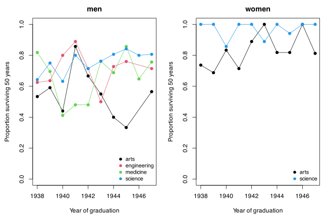
The plot backs this up: the year-to-year zig-zag is large but unsystematic, and the denominators behind the extreme points are tiny (Engineering 1943 is \(1\) of \(2\); several women’s Science cells have \(T \leq 5\)).
(b) Faculty, men. Restrict to men and test the four-level faculty factor against the minimal model.
men <- subset(g, sex == "men")
anova(glm(cbind(survive, died) ~ 1, binomial, data = men),
glm(cbind(survive, died) ~ faculty, binomial, data = men), test = "Chisq")
Analysis of Deviance Table
Model 1: cbind(survive, died) ~ 1
Model 2: cbind(survive, died) ~ faculty
Resid. Df Resid. Dev Df Deviance Pr(>Chi)
1 37 66.285
2 34 43.026 3 23.259 3.566e-05 ***
---
Signif. codes: 0 '***' 0.001 '**' 0.01 '*' 0.05 '.' 0.1 ' ' 1
\(\Delta D = 23.26\) on \(3\) df, \(p = 3.6 \times 10^{-5}\): the proportions are not the same across faculties. The odds ratios relative to Arts:
mb <- glm(cbind(survive, died) ~ faculty, binomial, data = men)
round(exp(cbind(OR = coef(mb), confint.default(mb))), 3)
OR 2.5 % 97.5 %
(Intercept) 1.211 0.893 1.640
facultyengineering 2.182 1.353 3.517
facultymedicine 1.492 1.009 2.207
facultyscience 2.710 1.747 4.202
Arts men fare worst (\(54.8\%\) surviving); Science men best (\(76.6\%\)), with \(2.7\) times the odds of surviving 50 years, and Engineering close behind at \(2.2\). Medicine sits between (\(64.4\%\), odds ratio \(1.49\), interval barely excluding 1). Adding faculty leaves \(D = 43.03\) on \(34\) df, an acceptable fit, and adding year on top changes nothing (\(\Delta D = 10.01\) on \(9\) df, \(p = 0.35\)), so the faculty ranking is not an artefact of different cohort mixes.
(c) Arts versus Science, women.
w <- subset(g, sex == "women")
anova(glm(cbind(survive, died) ~ 1, binomial, data = w),
glm(cbind(survive, died) ~ faculty, binomial, data = w), test = "Chisq")
Analysis of Deviance Table
Model 1: cbind(survive, died) ~ 1
Model 2: cbind(survive, died) ~ faculty
Resid. Df Resid. Dev Df Deviance Pr(>Chi)
1 19 22.555
2 18 13.739 1 8.8165 0.002985 **
---
Signif. codes: 0 '***' 0.001 '**' 0.01 '*' 0.05 '.' 0.1 ' ' 1
\(\Delta D = 8.82\) on \(1\) df, \(p = 0.003\): the proportions differ. Science women survived at \(58/61 = 95.1\%\) against \(126/157 = 80.3\%\) for Arts women, an odds ratio of \(\exp(1.5595) = 4.76\). The caveat is the size of the Science group – only 3 deaths in 61 – so the estimate is very imprecise (the Wald interval for the odds ratio runs from about \(1.4\) to \(16\)) even though the test itself is clear. This is exactly the small-expected-frequency situation Section 7.5 warns about, so I would quote the deviance test rather than the Wald \(z\) here.
(d) Sex difference: the same in Arts and Science? This is a test of the faculty-by-sex interaction on the two faculties where both sexes appear.
as2 <- droplevels(subset(g, faculty %in% c("arts", "science")))
anova(glm(cbind(survive, died) ~ faculty + sex, binomial, data = as2),
glm(cbind(survive, died) ~ faculty * sex, binomial, data = as2), test = "Chisq")
Analysis of Deviance Table
Model 1: cbind(survive, died) ~ faculty + sex
Model 2: cbind(survive, died) ~ faculty * sex
Resid. Df Resid. Dev Df Deviance Pr(>Chi)
1 36 31.153
2 35 30.358 1 0.79533 0.3725
\(\Delta D = 0.80\) on \(1\) df, \(p = 0.37\): no evidence of an interaction. By the algebra of Exercise 7.2(b), that means a single sex odds ratio describes both faculties. In the additive model
add <- glm(cbind(survive, died) ~ faculty + sex, binomial, data = as2)
round(exp(cbind(OR = coef(add), confint.default(add))), 3)
OR 2.5 % 97.5 %
(Intercept) 1.168 0.872 1.565
facultyscience 2.920 1.945 4.382
sexwomen 3.697 2.357 5.798
women have \(3.70\) times the odds of surviving 50 years that men do (\(95\%\) interval \(2.36\) to \(5.80\)), in Arts and in Science alike, and Science graduates have \(2.92\) times the odds of Arts graduates in both sexes. The additive model fits well, \(D = 31.15\) on \(36\) df (\(p = 0.70\)).
The separate estimates are \(\exp(0.9968) = 2.71\) (Science versus Arts among men) and \(\exp(1.5595) = 4.76\) (among women), which look different but differ by less than one standard error of the interaction term (\(0.563 \pm 0.664\)). On the probability scale the sex gap does look smaller in Science (\(0.951 - 0.766 = 0.19\)) than in Arts (\(0.803 - 0.548 = 0.26\)), but that is the usual squeeze of the logit scale near \(\pi = 1\), not evidence of interaction – the constant-odds-ratio model reproduces it. Power is also poor: with 61 women in Science, only a very large interaction would have been detectable, so “no interaction” here means “none demonstrated”, not “none present”.
Problem 7.4 — Let l(bmin ) denote the maximum value of the log-likelihood function for
Let \(l(\mathbf{b}_{\min})\) denote the maximum value of the log-likelihood function for the minimal model with linear predictor \(\mathbf{x}^T \boldsymbol{\beta} = \beta_1\), and let \(l(\mathbf{b})\) be the corresponding value for a more general model \(\mathbf{x}^T \boldsymbol{\beta} = \beta_1 + \beta_2 x_1 + \ldots + \beta_p x_{p-1}\).
a. Show that the likelihood ratio chi-squared statistic is \[ C = 2\left[l(\mathbf{b}) - l(\mathbf{b}_{\min})\right] = D_0 - D_1, \] where \(D_0\) is the deviance for the minimal model and \(D_1\) is the deviance for the more general model. b. Deduce that if \(\beta_2 = \ldots = \beta_p = 0\), then \(C\) has the central chi-squared distribution with \((p-1)\) degrees of freedom.
(difficulty: \(\star\star\))
(a) The deviance of any model is defined relative to the saturated (maximal) model, which has one parameter per covariate pattern and fitted probabilities \(\widehat{\pi}_i^{\max} = y_i/n_i\). Writing \(l(\mathbf{b}_{\max})\) for its maximised log-likelihood, the definition from Section 5.6.1 is \[ D = 2\left[l(\mathbf{b}_{\max}) - l(\mathbf{b})\right]. \] For the Binomial case this is exactly equation (7.5), \[ D = 2 \sum_{i=1}^{N} \left[ y_i \log\left(\frac{y_i}{\widehat{y}_i}\right) + (n_i - y_i)\log\left(\frac{n_i - y_i}{n_i - \widehat{y}_i}\right) \right], \] obtained by substituting \(\widehat{\pi}_i^{\max} = y_i/n_i\) and \(\widehat{\pi}_i = \widehat{y}_i/n_i\) into the log-likelihood (7.4). Note the feature the chapter stresses just below (7.5): \(D\) involves no nuisance parameter such as \(\sigma^2\), so no scaling is needed and the argument below is exact rather than approximate in that respect.
Apply the definition to the two models in question. The minimal model gives \[ D_0 = 2\left[l(\mathbf{b}_{\max}) - l(\mathbf{b}_{\min})\right], \] and the more general model gives \[ D_1 = 2\left[l(\mathbf{b}_{\max}) - l(\mathbf{b})\right]. \] Both are measured from the same reference point \(l(\mathbf{b}_{\max})\), because the saturated model does not depend on which of the two candidate models is under consideration. Subtracting, \[ D_0 - D_1 = 2\left[l(\mathbf{b}_{\max}) - l(\mathbf{b}_{\min})\right] - 2\left[l(\mathbf{b}_{\max}) - l(\mathbf{b})\right] = 2\left[l(\mathbf{b}) - l(\mathbf{b}_{\min})\right] = C, \] since the \(l(\mathbf{b}_{\max})\) terms cancel. This is the statistic defined in Section 7.5, \[ C = 2\left[l(\widehat{\boldsymbol{\pi}}; \mathbf{y}) - l(\widetilde{\boldsymbol{\pi}}; \mathbf{y})\right] = 2\sum\left[y_i \log\left(\frac{\widehat{y}_i}{n_i\widetilde{\pi}_i}\right) + (n_i - y_i)\log\left(\frac{n_i - \widehat{y}_i}{n_i - n_i\widetilde{\pi}_i}\right)\right], \] with \(\widetilde{\pi} = \left(\sum y_i\right)/\left(\sum n_i\right)\) the common probability under the minimal model. Two points are worth flagging. The cancellation needs the two models to be nested only in the weak sense that both are compared to the same saturated model – the identity \(C = D_0 - D_1\) is an algebraic identity that holds regardless. It is the distributional claim in (b) that needs the minimal model to be a special case of the general one.
A numerical confirmation using the Exercise 7.1 fit, where the two ways of computing \(C\) must agree to machine precision:
library(dobson)
data(hiroshima)
h <- hiroshima
names(h) <- c("dose", "leuk", "other", "total")
h$mid <- c(0, 5, 29.5, 74.5, 149.5, 300)
m1 <- glm(cbind(leuk, other) ~ mid, family = binomial, data = h)
m0 <- glm(cbind(leuk, other) ~ 1, family = binomial, data = h)
c(D0 = deviance(m0), D1 = deviance(m1), D0_minus_D1 = deviance(m0) - deviance(m1),
C_loglik = 2 * (as.numeric(logLik(m1)) - as.numeric(logLik(m0))))
D0 D1 D0_minus_D1 C_loglik
54.3508862 0.6795634 53.6713228 53.6713228
(b) Suppose the minimal model is correct, i.e. \(\beta_2 = \ldots = \beta_p = 0\). Then both fitted models are correct, so the sampling distribution for the deviance derived in Section 5.6 applies to each (the pointer printed alongside the definition of \(C\) in Section 7.5 reads “Section 5.2”, but the deviance result being invoked is the one in Section 5.6, and the difference-of-deviances argument is Section 5.7): \[ D_0 \sim \chi^2(N - 1), \qquad D_1 \sim \chi^2(N - p), \] asymptotically, where \(N\) is the number of covariate patterns, the minimal model estimates \(1\) parameter and the general model \(p\).
Now decompose \[ D_0 = D_1 + C. \] The standard asymptotic argument writes each deviance as a quadratic form in asymptotically Normal quantities, via the Taylor expansion used in Section 5.6: \(D_0\) is the squared length of the residual vector projected onto the orthogonal complement of the one-dimensional model space, and \(D_1\) the projection onto the orthogonal complement of the \(p\)-dimensional space, which contains the former. Because the two projections are nested, \(C = D_0 - D_1\) is the squared length of the projection onto the \((p-1)\)-dimensional difference of the spaces, and it is independent of \(D_1\). This is the “certain independence conditions” that Section 5.7 attaches to the result \(\Delta D \sim \chi^2(p-q)\), referring back to Section 1.5 on quadratic forms; it is the Binomial-likelihood analogue of the orthogonal decomposition of sums of squares for Normal linear models. Hence, by the additivity of independent chi-squared variables, \[ C \sim \chi^2\left((N-1) - (N-p)\right) = \chi^2(p-1). \] The distribution is central precisely because the minimal model is true, so the mean of the projected residual vector in the \((p-1)\)-dimensional difference space is zero. Equivalently, this is Wilks’ theorem: \(C\) is twice the log-likelihood ratio for the \((p-1)\) constraints \(\beta_2 = \ldots = \beta_p = 0\), and under those constraints \(C \to \chi^2(p-1)\).
If instead \(\beta_2, \ldots, \beta_p\) are not all zero, the general model is still correct so \(D_1 \sim \chi^2(N-p)\), but \(D_0\) has a non-central distribution and so does \(C\), with non-centrality parameter growing with \(\|\boldsymbol{\beta}_{2:p}\|\) evaluated in the metric of the information matrix. That is exactly the property that makes \(C\) a test statistic: it is stochastically larger under alternatives, so large values are evidence against the minimal model, which is how the drop of \(53.67\) in the fit above was read.
One honest caveat: all of this is asymptotic. Both the chi-squared approximation to \(D_1\) and the independence of \(C\) and \(D_1\) are large-sample statements; the chapter notes after (7.5) that they can be poor when expected frequencies are small (say below 1). The distribution of \(C\) tends to be the more reliable of the two, because it compares two fitted models with the same data and does not require the number of covariate patterns to stay fixed as \(n\) grows – which is why \(C\) is usable even for ungrouped binary data (\(n_i = 1\)) where \(D_1\) itself is not a valid goodness-of-fit statistic at all.
Simulation check of (b): 5000 data sets generated under the minimal model (\(\pi = 0.3\) for all 40 covariate patterns), with \(C\) computed against a general model with \(p = 3\). The claim is \(C \sim \chi^2(2)\), i.e. mean 2, variance 4, upper 5% point 5.99.
set.seed(2026)
n <- rep(30, 40)
x1 <- rnorm(40)
x2 <- rnorm(40)
C <- replicate(5000, {
y <- rbinom(40, n, 0.3)
m0 <- glm(cbind(y, n - y) ~ 1, binomial)
m1 <- glm(cbind(y, n - y) ~ x1 + x2, binomial)
deviance(m0) - deviance(m1)
})
round(c(mean = mean(C), var = var(C), q95 = quantile(C, 0.95),
chisq2_mean = 2, chisq2_var = 4, chisq2_q95 = qchisq(0.95, 2)), 3)
mean var q95.95% chisq2_mean chisq2_var chisq2_q95
2.027 4.227 6.089 2.000 4.000 5.991
Mean, variance and upper percentile all match \(\chi^2(2)\) closely.
Problem 7.5 — Let Yi be the number of successes in ni trials with
Let \(Y_i\) be the number of successes in \(n_i\) trials with \[ Y_i \sim \text{Bin}(n_i, \pi_i), \] where the probabilities \(\pi_i\) have a Beta distribution \[ \pi_i \sim \text{Be}(\alpha, \beta). \] The probability density function for the Beta distribution is \(f(x; \alpha, \beta) = x^{\alpha-1}(1-x)^{(\beta-1)}/B(\alpha, \beta)\) for \(x\) in \([0, 1]\), \(\alpha > 0\), \(\beta > 0\) and the beta function \(B(\alpha, \beta)\) defining the normalizing constant required to ensure that \(\int_0^1 f(x; \alpha, \beta)\,dx = 1\). It can be shown that \(E(X) = \alpha/(\alpha+\beta)\) and \(\text{var}(X) = \alpha\beta/[(\alpha+\beta)^2(\alpha+\beta+1)]\). Let \(\theta = \alpha/(\alpha+\beta)\), and hence, show that
a. \(E(\pi_i) = \theta\) b. \(\text{var}(\pi_i) = \theta(1-\theta)/(\alpha+\beta+1) = \phi\,\theta(1-\theta)\) c. \(E(Y_i) = n_i\theta\) d. \(\text{var}(Y_i) = n_i\theta(1-\theta)[1 + (n_i - 1)\phi]\) so that \(\text{var}(Y_i)\) is larger than the Binomial variance (unless \(n_i = 1\) or \(\phi = 0\)).
(difficulty: \(\star\star\))
This is the beta-binomial model, the standard construction for overdispersed Binomial data: the success probability is not fixed at \(\pi_i\) but varies from unit to unit, and part (d) quantifies exactly how much extra variance that variation injects. Throughout, write \(\phi = 1/(\alpha + \beta + 1)\), so that \(0 < \phi < 1\) for all admissible \(\alpha, \beta > 0\).
(a) Immediate from the quoted mean of the Beta distribution with \(X = \pi_i\): \[ E(\pi_i) = \frac{\alpha}{\alpha+\beta} = \theta. \]
(b) Start from the quoted variance and rewrite it in terms of \(\theta\). Since \(\theta = \alpha/(\alpha+\beta)\) we have \(1 - \theta = \beta/(\alpha+\beta)\), and therefore \[ \theta(1-\theta) = \frac{\alpha}{\alpha+\beta}\cdot\frac{\beta}{\alpha+\beta} = \frac{\alpha\beta}{(\alpha+\beta)^2}. \] Hence \[ \text{var}(\pi_i) = \frac{\alpha\beta}{(\alpha+\beta)^2(\alpha+\beta+1)} = \frac{1}{\alpha+\beta+1}\cdot\frac{\alpha\beta}{(\alpha+\beta)^2} = \frac{\theta(1-\theta)}{\alpha+\beta+1} = \phi\,\theta(1-\theta). \] So \(\phi\) measures the spread of the \(\pi_i\) relative to the largest spread a random variable on \([0,1]\) with mean \(\theta\) could have. As \(\alpha + \beta \to \infty\) with \(\theta\) fixed, \(\phi \to 0\) and the Beta distribution collapses onto the point \(\theta\); as \(\alpha + \beta \to 0\), \(\phi \to 1\) and \(\pi_i\) becomes a two-point distribution on \(\{0, 1\}\).
(c) Use the tower property (iterated expectation). Conditionally, \(E(Y_i \mid \pi_i) = n_i\pi_i\) from the Binomial mean, so \[ E(Y_i) = E\left[E(Y_i \mid \pi_i)\right] = E(n_i\pi_i) = n_i E(\pi_i) = n_i\theta, \] using (a). The marginal mean is therefore unchanged by the mixing – the beta-binomial has the same mean structure as the Binomial, which is what makes it a pure overdispersion model.
(d) Use the conditional variance decomposition \[ \text{var}(Y_i) = E\left[\text{var}(Y_i \mid \pi_i)\right] + \text{var}\left[E(Y_i \mid \pi_i)\right]. \] The two conditional Binomial moments are \(\text{var}(Y_i \mid \pi_i) = n_i\pi_i(1-\pi_i)\) and \(E(Y_i \mid \pi_i) = n_i\pi_i\), so \[ \text{var}(Y_i) = n_i E\left[\pi_i(1-\pi_i)\right] + n_i^2\,\text{var}(\pi_i). \] For the first term, \(E[\pi_i(1-\pi_i)] = E(\pi_i) - E(\pi_i^2)\) and \(E(\pi_i^2) = \text{var}(\pi_i) + [E(\pi_i)]^2 = \phi\theta(1-\theta) + \theta^2\). Hence \[ E\left[\pi_i(1-\pi_i)\right] = \theta - \theta^2 - \phi\theta(1-\theta) = \theta(1-\theta)\left[1 - \phi\right]. \] Substituting both terms, \[ \text{var}(Y_i) = n_i\theta(1-\theta)(1-\phi) + n_i^2\phi\theta(1-\theta) = n_i\theta(1-\theta)\left[1 - \phi + n_i\phi\right] = n_i\theta(1-\theta)\left[1 + (n_i-1)\phi\right], \] which is the required result.
The overdispersion statement. The Binomial variance with the same mean is \(n_i\theta(1-\theta)\), so the beta-binomial variance exceeds it by the factor \[ 1 + (n_i - 1)\phi \geq 1, \] with equality if and only if \((n_i - 1)\phi = 0\), i.e. \(n_i = 1\) or \(\phi = 0\). Both edge cases have a transparent reading. If \(n_i = 1\) then \(Y_i\) is Bernoulli with marginal success probability \(\theta\), and a Bernoulli variable is completely determined by its mean – there is no room for extra variance, so binary (ungrouped) data can never exhibit overdispersion of this kind, no matter how heterogeneous the \(\pi_i\) are. If \(\phi = 0\) the \(\pi_i\) are degenerate at \(\theta\) and the model reduces exactly to \(\text{Bin}(n_i, \theta)\). Strictly, \(\phi = 0\) is not attainable for finite \(\alpha, \beta > 0\); it is the limit \(\alpha + \beta \to \infty\). So for any genuine Beta mixing and any \(n_i > 1\) the inequality is strict.
Note the practical consequence, which is why the exercise is here. Fitting an ordinary Binomial GLM to beta-binomial data leaves the estimates of \(\theta\) (and of regression coefficients through it) consistent, because (c) says the mean model is unaffected, but it understates the variance by the factor \(1 + (n_i - 1)\phi\). Standard errors are then too small, the deviance (7.5) and \(X^2\) (7.6) are inflated relative to \(\chi^2(N-p)\), and the goodness-of-fit test rejects models that are correct in the mean. The factor grows with \(n_i\), so overdispersion is most damaging where the group sizes are largest. The usual remedies are to estimate a dispersion parameter and scale the standard errors (quasi-binomial), or to fit the beta-binomial likelihood directly.
Numerical check. The algebra in (d) is easy to mis-collect, so simulate with \(\alpha = 2\), \(\beta = 3\), \(n = 20\): then \(\theta = 0.4\), \(\phi = 1/6\), the predicted \(\text{var}(\pi) = 0.04\), \(E(Y) = 8\), and \(\text{var}(Y) = 20 \times 0.24 \times (1 + 19/6) = 20\), against a Binomial variance of \(4.8\).
set.seed(7)
alpha <- 2; beta <- 3; n <- 20
theta <- alpha / (alpha + beta)
phi <- 1 / (alpha + beta + 1)
p <- rbeta(2e6, alpha, beta)
y <- rbinom(2e6, n, p)
round(c(theta = theta, mean_pi = mean(p),
var_pi_theory = phi * theta * (1 - theta), var_pi_sim = var(p),
EY_theory = n * theta, EY_sim = mean(y),
varY_theory = n * theta * (1 - theta) * (1 + (n - 1) * phi), varY_sim = var(y),
binomial_var = n * theta * (1 - theta)), 4)
theta mean_pi var_pi_theory var_pi_sim EY_theory
0.4000 0.3998 0.0400 0.0400 8.0000
EY_sim varY_theory varY_sim binomial_var
7.9972 20.0000 20.0048 4.8000
Every simulated moment matches its formula, and the realised variance of \(Y\) is more than four times the Binomial value – the overdispersion factor \(1 + 19/6 = 4.17\).
Nominal and Ordinal Logistic Regression
Problem 8.1 — If there are only J = 2 response categories, show that models (8.4), (8.13),
If there are only \(J = 2\) response categories, show that models (8.4), (8.13), (8.15) and (8.16) all reduce to the logistic regression model for binary data. (difficulty: \(\star\))
Throughout put \(J = 2\), so the response has categories \(1\) and \(2\) with probabilities \(\pi_1\) and \(\pi_2 = 1 - \pi_1\). Section 8.2 has already disposed of the distributional half of the question: for \(J = 2\) the Multinomial distribution (8.1) is \(\mathrm{M}(n, \pi_1, \pi_2)\) with \(\pi_2 = 1 - \pi_1\) and \(y_2 = n - y_1\), which is exactly the Binomial distribution \(\mathrm{B}(n, \pi_1)\) of (7.1). So only the systematic component has to be checked, and each of the four models specifies exactly one equation when \(J = 2\) (there are \(J-1 = 1\) non-redundant logits).
Nominal logistic regression, model (8.4). The equations are indexed by \(j = 2, \ldots, J\), so there is a single one, \(j = 2\):
\begin{equation*} \log\left(\frac{\pi_2}{\pi_1}\right) = \mathbf{x}_2^T\boldsymbol{\beta}_2 \quad\Longleftrightarrow\quad \log\left(\frac{\pi_2}{1 - \pi_2}\right) = \mathbf{x}_2^T\boldsymbol{\beta}_2 , \end{equation*}
using \(\pi_1 = 1 - \pi_2\). This is the logistic regression model of Section 7.2 with category \(2\) playing the role of “success”. Equivalently \(\mathrm{logit}(\pi_1) = -\mathbf{x}_2^T\boldsymbol{\beta}_2\): choosing the other reference category only reverses the sign of every parameter.
Cumulative logit model, model (8.13). The cutpoints are \(C_1, \ldots, C_{J-1}\), so with \(J = 2\) there is one cutpoint and one equation, \(j = 1\):
\begin{equation*} \log\left(\frac{\pi_1}{\pi_2}\right) = \log\left(\frac{\pi_1}{1 - \pi_1}\right) = \mathbf{x}_1^T\boldsymbol{\beta}_1 , \end{equation*}
again binary logistic regression, now with category \(1\) as “success”. The proportional odds specialisation (8.14) is the same equation with \(\beta_{0j}\) collapsing to a single intercept \(\beta_{01}\); with only one cutpoint the proportional odds assumption is vacuous, since there is nothing for the odds to be proportional across. This is why software refuses the fit: MASS::polr stops with “response must have 3 or more levels”.
Adjacent category logit model, model (8.15). The ratios \(\pi_1/\pi_2, \ldots, \pi_{J-1}/\pi_J\) collapse to the single ratio \(\pi_1/\pi_2\), so
\begin{equation*} \log\left(\frac{\pi_1}{\pi_2}\right) = \log\left(\frac{\pi_1}{1 - \pi_1}\right) = \mathbf{x}_1^T\boldsymbol{\beta}_1 . \end{equation*}
“Adjacent” and “cumulative” coincide because with two categories the only adjacent pair is also the only split of the scale.
Continuation ratio logit model, model (8.16). The denominator \(\pi_{j+1} + \ldots + \pi_J\) reduces to \(\pi_2\) when \(j = 1\), so
\begin{equation*} \log\left(\frac{\pi_1}{\pi_2}\right) = \log\left(\frac{\pi_1}{1 - \pi_1}\right) = \mathbf{x}_1^T\boldsymbol{\beta}_1 . \end{equation*}
The conditioning event \(z > C_{j-1}\) is empty for \(j = 1\), so no conditioning is imposed and the model is unconditional.
Hence all four are the single equation \(\mathrm{logit}(\pi) = \mathbf{x}^T\boldsymbol{\beta}\); they differ only in which of the two categories is put in the numerator, which changes the sign of \(\boldsymbol{\beta}\) and nothing else. The distinctions between the four models are distinctions about the way the \(J-1\) logits are formed, and for \(J = 2\) there is only one logit to form.
A numerical check on the beetle mortality data of Section 7.3, which is genuinely binary (killed / survived), fitting all four multicategory models plus the ordinary binomial GLM:
library(dobson)
library(nnet)
library(VGAM)
data(beetle)
Y <- cbind(killed = beetle$y, survived = beetle$n - beetle$y)
b <- data.frame(x = rep(beetle$x, 2),
resp = factor(rep(c("killed", "survived"), each = nrow(beetle)),
levels = c("killed", "survived")),
freq = c(beetle$y, beetle$n - beetle$y))
m.glm <- glm(cbind(y, n - y) ~ x, family = binomial, data = beetle)
m.nom <- multinom(resp ~ x, weights = freq, data = b, trace = FALSE,
maxit = 1000, reltol = 1e-14)
m.cum <- vglm(Y ~ x, cumulative(parallel = TRUE), data = beetle)
# reverse = TRUE gives the book's log(pi_j / pi_{j+1}); sratio gives the book's (8.16)
m.acat <- vglm(Y ~ x, acat(reverse = TRUE, parallel = TRUE), data = beetle)
m.srat <- vglm(Y ~ x, sratio(reverse = FALSE, parallel = TRUE), data = beetle)
tab <- rbind("binomial glm: logit P(killed)" = coef(m.glm),
"(8.4) nominal, log(pi2/pi1)" = coef(m.nom),
"(8.13) cumulative logit" = coef(m.cum),
"(8.15) adjacent category" = coef(m.acat),
"(8.16) continuation ratio" = coef(m.srat))
colnames(tab) <- c("intercept", "slope")
round(tab, 4)
intercept slope
binomial glm: logit P(killed) -60.7175 34.2703
(8.4) nominal, log(pi2/pi1) 60.7175 -34.2703
(8.13) cumulative logit -60.7175 34.2703
(8.15) adjacent category -60.7175 34.2703
(8.16) continuation ratio -60.7175 34.2703
Every fit reproduces \(|\hat\beta_1| = 60.7175\) and \(|\hat\beta_2| = 34.2703\) to all printed digits, and once each model is written with the book’s category in the numerator all four agree in sign as well; only the nominal model (8.4), which by construction puts the non-reference category on top, has the opposite sign.
Problem 8.2 — The data in Table 8.5 are from an investigation into satisfaction with hous-
The data in Table 8.5 are from an investigation into satisfaction with housing conditions in Copenhagen (derived from Example W in Cox and Snell, 1981, from original data from Madsen, 1971). Residents in selected areas living in rented homes built between 1960 and 1968 were questioned about their satisfaction and the degree of contact with other residents. The data were tabulated by type of housing.
Table 8.5, satisfaction with housing conditions. The rows are the three types of housing and the columns are the six combinations of satisfaction (low, medium, high) with degree of contact with other residents (low, high), the counts being read across as (low satisfaction: low contact, high contact), (medium satisfaction: low contact, high contact), (high satisfaction: low contact, high contact). Tower block: 65, 34, 54, 47, 100, 100. Apartment: 130, 141, 76, 116, 111, 191. House: 67, 130, 48, 105, 62, 104.
a. Summarize the data using appropriate tables of percentages to show the associations between levels of satisfaction and contact with other residents, levels of satisfaction and type of housing, and contact and type of housing.
b. Use nominal logistic regression to model associations between level of satisfaction and the other two variables. Obtain a parsimonious model that summarizes the patterns in the data.
c. Do you think an ordinal model would be appropriate for associations between the levels of satisfaction and the other variables? Justify your answer. If you consider such a model to be appropriate, fit a suitable one and compare the results with those from (b).
d. From the best model you obtained in (c), calculate the standardized residuals and use them to find where the largest discrepancies are between the observed frequencies and expected frequencies estimated from the model. (difficulty: \(\star\star\star\))
The data ship with the dobson package as housing. One trap: MASS also exports a data set called housing (Copenhagen again, but with an extra “influence” factor and \(72\) rows), and MASS has to be loaded for polr, so every block below calls data(housing, package = "dobson") explicitly.
Part (a). Three two-way marginal tables of row percentages.
library(dobson)
data(housing, package = "dobson")
housing$satisfaction <- factor(housing$satisfaction, levels = c("low", "medium", "high"))
housing$contact <- factor(housing$contact, levels = c("low", "high"))
housing$type <- factor(housing$type, levels = c("tower block", "apartment", "house"))
tab <- xtabs(frequency ~ type + contact + satisfaction, data = housing)
round(100 * prop.table(margin.table(tab, c(2, 3)), 1), 1) # satisfaction by contact
satisfaction
contact low medium high
low 36.7 25.0 38.3
high 31.5 27.7 40.8
round(100 * prop.table(margin.table(tab, c(1, 3)), 1), 1) # satisfaction by type of housing
satisfaction
type low medium high
tower block 24.8 25.2 50.0
apartment 35.4 25.1 39.5
house 38.2 29.7 32.2
round(100 * prop.table(margin.table(tab, c(1, 2)), 1), 1) # contact by type of housing
contact
type low high
tower block 54.8 45.2
apartment 41.4 58.6
house 34.3 65.7
round(100 * prop.table(ftable(tab, row.vars = c(1, 2)), 1), 1)
satisfaction low medium high
type contact
tower block low 29.7 24.7 45.7
high 18.8 26.0 55.2
apartment low 41.0 24.0 35.0
high 31.5 25.9 42.6
house low 37.9 27.1 35.0
high 38.3 31.0 30.7
margin.table(tab, c(1, 2))
contact
type low high
tower block 219 181
apartment 317 448
house 177 339
Reading the three marginal tables. Satisfaction rises with contact, but only mildly: high satisfaction goes from \(38.3\%\) to \(40.8\%\) and low satisfaction falls from \(36.7\%\) to \(31.5\%\). Satisfaction depends strongly on housing type: high satisfaction is \(50.0\%\) in tower blocks, \(39.5\%\) in apartments and \(32.2\%\) in houses, a monotone decline, with low satisfaction moving the opposite way (\(24.8\%\), \(35.4\%\), \(38.2\%\)). Contact also depends on type: high contact is reported by \(45.2\%\) of tower-block residents, \(58.6\%\) in apartments and \(65.7\%\) in houses. Note that the last association runs against the first two, so the crude satisfaction-by-contact margin understates the contact effect: houses have both the most contact and the least satisfaction, and the two effects partly cancel in the margin. The full six-row table confirms this. Within tower blocks, high contact raises the proportion “highly satisfied” from \(45.7\%\) to \(55.2\%\); within apartments from \(35.0\%\) to \(42.6\%\); but within houses it falls slightly, \(35.0\%\) to \(30.7\%\). That non-parallel behaviour in the houses row is the only hint of an interaction.
pr <- prop.table(tab, c(1, 2))
par(mfrow = c(1, 2), mar = c(4, 4, 3, 1))
for (k in c("low", "high")) {
plot(0, 0, type = "n", xlim = c(1, 3), ylim = c(0, 0.6), xaxt = "n",
xlab = "satisfaction", ylab = "proportion",
main = paste("contact with other residents:", k))
axis(1, at = 1:3, labels = c("low", "medium", "high"))
for (i in 1:3)
lines(1:3, pr[i, k, ], type = "b", lty = i, pch = 14 + i, lwd = 2)
legend("topleft", legend = dimnames(pr)$type, lty = 1:3, pch = 15:17, lwd = 2, bty = "n")
}
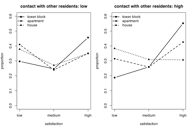
Part (b). Treat satisfaction as nominal with three categories, “low” as reference, and fit model (8.4) with multinom. There are \(3 \times 2 = 6\) covariate patterns, so the maximal model has \(6\) parameters for each of the \(J - 1 = 2\) logits, \(12\) in all; deviances (8.7) are taken against that.
library(nnet)
f <- function(rhs) multinom(rhs, weights = frequency, data = housing, trace = FALSE,
maxit = 1000, reltol = 1e-14)
mods <- list(minimal = f(satisfaction ~ 1), contact = f(satisfaction ~ contact),
type = f(satisfaction ~ type), `type+contact` = f(satisfaction ~ type + contact),
`type*contact` = f(satisfaction ~ type * contact))
lsat <- as.numeric(logLik(mods[["type*contact"]]))
out <- t(sapply(mods, function(m) c(npar = length(coef(m)), logLik = as.numeric(logLik(m)),
deviance = 2 * (lsat - as.numeric(logLik(m))),
df = 12 - length(coef(m)), AIC = AIC(m))))
round(cbind(out, p = pchisq(out[, "deviance"], out[, "df"], lower.tail = FALSE)), 4)
npar logLik deviance df AIC p
minimal 2 -1824.439 50.2903 10 3652.878 0.0000
contact 4 -1821.876 45.1645 8 3651.752 0.0000
type 6 -1807.174 15.7608 6 3626.348 0.0151
type+contact 8 -1802.740 6.8930 4 3621.480 0.1417
type*contact 12 -1799.294 0.0000 0 3622.587 1.0000
The additive model has deviance \(D = 6.89\) on \(4\) degrees of freedom (\(p = 0.14\)), so it describes the six covariate patterns adequately; adding the interaction buys \(6.89\) on \(4\) df and raises AIC (8.10) from \(3621.5\) to \(3622.6\). Dropping either main effect is not permissible: removing contact costs \(15.76 - 6.89 = 8.87\) on \(2\) df (\(p = 0.012\)) and removing type costs \(45.17 - 6.89 = 38.27\) on \(4\) df (\(p < 10^{-7}\)). The parsimonious nominal model is therefore
\begin{equation*} \log\left(\frac{\pi_j}{\pi_1}\right) = \beta_{0j} + \beta_{1j}x_1 + \beta_{2j}x_2 + \beta_{3j}x_3, \qquad j = 2, 3, \end{equation*}
with \(j = 1, 2, 3\) for low, medium and high satisfaction, \(x_1 = 1\) for apartment, \(x_2 = 1\) for house (tower block the reference) and \(x_3 = 1\) for high contact.
mtc <- multinom(satisfaction ~ type + contact, weights = frequency, data = housing,
trace = FALSE, maxit = 1000, reltol = 1e-14)
s <- summary(mtc)
res <- cbind(b = as.vector(t(s$coefficients)), se = as.vector(t(s$standard.errors)))
rownames(res) <- paste(rep(rownames(s$coefficients), each = ncol(s$coefficients)),
colnames(s$coefficients), sep = ": ")
round(cbind(res, z = res[, 1] / res[, 2], OR = exp(res[, 1]),
lo = exp(res[, 1] - 1.96 * res[, 2]), hi = exp(res[, 1] + 1.96 * res[, 2])), 3)
b se z OR lo hi
medium: (Intercept) -0.107 0.152 -0.704 0.898 0.666 1.211
medium: typeapartment -0.407 0.171 -2.375 0.666 0.476 0.931
medium: typehouse -0.337 0.180 -1.869 0.714 0.501 1.017
medium: contacthigh 0.296 0.130 2.275 1.344 1.042 1.735
high: (Intercept) 0.561 0.133 4.219 1.752 1.350 2.273
high: typeapartment -0.642 0.150 -4.275 0.526 0.392 0.706
high: typehouse -0.946 0.164 -5.749 0.388 0.281 0.536
high: contacthigh 0.328 0.118 2.777 1.389 1.101 1.750
Interpretation. Relative to a tower block, the odds of being highly rather than lowly satisfied are multiplied by \(0.53\) (\(95\%\) CI \(0.39\) to \(0.71\)) in an apartment and by \(0.39\) (\(0.28\) to \(0.54\)) in a house; the corresponding odds ratios for medium versus low satisfaction are \(0.67\) and \(0.71\). High contact with other residents multiplies the odds of high versus low satisfaction by \(1.39\) (\(1.10\) to \(1.75\)) and of medium versus low by \(1.34\) (\(1.04\) to \(1.74\)). The pattern worth noticing is that within each explanatory variable the two odds ratios line up in order: for type the “high versus low” ratio is further from \(1\) than the “medium versus low” ratio (\(0.53 < 0.67\), \(0.39 < 0.71\)), while for contact the two are almost equal (\(1.39\) against \(1.34\)). That is precisely the monotone ordering an ordinal model imposes.
Part (c). An ordinal model is appropriate. Satisfaction low \(<\) medium \(<\) high is a genuine ordering of a single underlying attitude, exactly the latent-variable picture of Figure 8.2, and the estimates in (b) already behave as an ordinal model predicts: the effect of every explanatory variable on the “medium versus low” logit has the same sign as its effect on the “high versus low” logit, and the effects grow with the response category. Fitting the proportional odds model (8.14),
\begin{equation*} \log\left(\frac{\pi_1 + \ldots + \pi_j}{\pi_{j+1} + \ldots + \pi_J}\right) = \beta_{0j} + \beta_1 x_1 + \beta_2 x_2 + \beta_3 x_3, \qquad j = 1, 2 , \end{equation*}
costs three parameters instead of six and buys back three degrees of freedom.
library(MASS)
housing$satisfaction <- ordered(housing$satisfaction, levels = c("low", "medium", "high"))
p1 <- polr(satisfaction ~ type + contact, weights = frequency, data = housing, Hess = TRUE)
summary(p1)
Call:
polr(formula = satisfaction ~ type + contact, data = housing,
weights = frequency, Hess = TRUE)
Coefficients:
Value Std. Error t value
typeapartment -0.5009 0.11675 -4.291
typehouse -0.7362 0.12610 -5.838
contacthigh 0.2524 0.09306 2.713
Intercepts:
Value Std. Error t value
low|medium -0.9973 0.1075 -9.2794
medium|high 0.1152 0.1047 1.1004
Residual Deviance: 3610.286
AIC: 3620.286
c(polr = as.numeric(logLik(p1)), nominal = as.numeric(logLik(mtc)), saturated = lsat)
polr nominal saturated
-1805.143 -1802.740 -1799.294
anova(p1, polr(satisfaction ~ type * contact, weights = frequency, data = housing))
Likelihood ratio tests of ordinal regression models
Response: satisfaction
Model Resid. df Resid. Dev Test Df LR stat. Pr(Chi)
1 type + contact 1676 3610.286
2 type * contact 1674 3604.091 1 vs 2 2 6.195546 0.04514963
Note that polr parameterises the cumulative logit as \(\beta_{0j} - \boldsymbol{\beta}^T\mathbf{x}\), so the printed coefficients have the sign of an effect on the upper end of the scale; a positive coefficient means more satisfaction. Comparison with the maximal model gives \(D = 2(-1799.294 + 1805.143) = 11.70\) on \(12 - 5 = 7\) degrees of freedom, \(p = 0.11\), so the proportional odds model fits. Comparing it with the nominal model of (b) tests the proportional odds assumption directly: \(\Delta D = 2(-1802.740 + 1805.143) = 4.81\) on \(8 - 5 = 3\) df, \(p = 0.19\), no evidence against proportional odds. AIC also prefers the ordinal model (\(3620.3\) against \(3621.5\)). This is the same conclusion as in the car preference example of Section 8.4.6: the two models describe the data equally well and the ordinal one is chosen for parsimony and for using the order of the categories.
The estimates say that, relative to a tower block, the odds of being at or below any given satisfaction level are multiplied by \(e^{0.5009} = 1.65\) for an apartment and \(e^{0.7362} = 2.09\) for a house (equivalently, apartments and houses shift residents down the satisfaction scale), and high contact multiplies the odds of being above any given level by \(e^{0.2524} = 1.29\) (\(95\%\) CI \(1.07\) to \(1.55\)). Each of these is a compromise between the pair of nominal odds ratios it replaces (for example \(e^{-0.5009} = 0.61\) for an apartment against the nominal pair \(0.67\) and \(0.53\)), which is why the two fits are so similar.
One caveat, stated because it cuts against the tidy answer. Within the proportional odds family the type-by-contact interaction is borderline significant, \(\Delta D = 6.20\) on \(2\) df, \(p = 0.045\), and lowers AIC from \(3620.3\) to \(3618.1\). In the nominal family the same interaction was not significant (\(p = 0.14\)), so the evidence is weak and depends on the model family; I keep the additive model as “best” for parsimony, but part (d) shows exactly where the interaction would act.
Part (d). Expected frequencies are the fitted probabilities from the additive proportional odds model multiplied by the total for each covariate pattern; the standardized (Pearson) residuals are \(r_i = (o_i - e_i)/\sqrt{e_i}\) from (8.5).
pat <- unique(housing[, c("type", "contact")])
n <- aggregate(frequency ~ type + contact, data = housing, sum)
prob <- predict(p1, newdata = pat, type = "probs")
tot <- n$frequency[match(paste(pat$type, pat$contact), paste(n$type, n$contact))]
long <- reshape(data.frame(pat, tot * prob), direction = "long", varying = list(3:5),
v.names = "expected", timevar = "satisfaction",
times = c("low", "medium", "high"), idvar = c("type", "contact"))
res <- merge(housing, long, by = c("type", "contact", "satisfaction"))
res$satisfaction <- factor(res$satisfaction, levels = c("low", "medium", "high"))
res <- res[order(res$type, res$contact, res$satisfaction), ]
res$r <- (res$frequency - res$expected) / sqrt(res$expected)
rownames(res) <- NULL
data.frame(res[, c("type", "contact", "satisfaction", "frequency")],
expected = round(res$expected, 2), r = round(res$r, 3))
type contact satisfaction frequency expected r
1 tower block low low 65 59.01 0.779
2 tower block low medium 54 56.79 -0.370
3 tower block low high 100 103.20 -0.315
4 tower block high low 34 40.32 -0.995
5 tower block high medium 47 43.98 0.455
6 tower block high high 100 96.70 0.335
7 apartment low low 130 119.95 0.918
8 apartment low medium 76 85.89 -1.067
9 apartment low high 111 111.16 -0.015
10 apartment high low 141 143.84 -0.237
11 apartment high medium 116 120.45 -0.405
12 apartment high high 191 183.71 0.538
13 house low low 67 77.01 -1.141
14 house low medium 48 47.04 0.140
15 house low high 62 52.95 1.244
16 house high low 130 126.91 0.274
17 house high medium 105 91.89 1.368
18 house high high 104 120.20 -1.478
sum(res$r^2)
[1] 11.64202
The chi-squared statistic (8.6) is \(X^2 = 11.64\), close to the deviance \(D = 11.70\) as it should be, and consistent with \(\chi^2(7)\) (\(p = 0.11\)): no residual is anywhere near \(2\) in absolute value, so no cell is badly fitted.
The largest discrepancies are all in the “house” rows and all concern the effect of contact. For houses with high contact the model predicts \(120.2\) highly satisfied residents but only \(104\) were observed (\(r = -1.48\)), the deficit reappearing as an excess of medium satisfaction (\(105\) against \(91.9\), \(r = 1.37\)). For houses with low contact the reverse holds: \(62\) highly satisfied against \(53.0\) predicted (\(r = 1.24\)) and a shortfall at low satisfaction (\(67\) against \(77.0\), \(r = -1.14\)). In words, the model imposes the same positive contact effect on every housing type, but among house dwellers contact is associated with slightly less satisfaction, not more (the row percentages in (a): \(35.0\%\) highly satisfied at low contact against \(30.7\%\) at high contact). That is exactly the type-by-contact interaction flagged at the end of (c). The next largest residuals, in the apartment low-contact row (\(r = 0.92\) and \(-1.07\)), are an ordinary medium-versus-low reshuffle and carry no interpretation. Given that the overall fit is acceptable and the interaction is only marginally significant, the honest reading is that the additive model is adequate but that any real departure from it lives in the house-by-contact cells.
Problem 8.3 — The data in Table 8.6 show tumor responses of male and female patients
The data in Table 8.6 show tumor responses of male and female patients receiving treatment for small-cell lung cancer. There were two treatment regimes. For the sequential treatment, the same combination of chemotherapeutic agents was administered at each treatment cycle. For the alternating treatment, different combinations were alternated from cycle to cycle (data from Holtbrugger and Schumacher, 1991).
Table 8.6, tumor responses to two different treatments, numbers of patients in each category. The columns are progressive disease, no change, partial remission, complete remission. Sequential treatment, male: 28, 45, 29, 26; sequential, female: 4, 12, 5, 2. Alternating treatment, male: 41, 44, 20, 20; alternating, female: 12, 7, 3, 1.
a. Fit a proportional odds model to estimate the probabilities for each response category taking treatment and sex effects into account.
b. Examine the adequacy of the model fitted in (a) using residuals and goodness of fit statistics.
c. Use a Wald statistic to test the hypothesis that there is no difference in responses for the two treatment regimes.
d. Fit two proportional odds models to test the hypothesis of no treatment difference. Compare the results with those for (c) above.
e. Fit adjacent category models and continuation ratio models using logit, probit and complementary log-log link functions. How do the different models affect the interpretation of the results? (difficulty: \(\star\star\star\))
The data ship with the dobson package as tumor. Order the response progressive disease \(<\) no change \(<\) partial remission \(<\) complete remission, so that “large” means a good outcome, and take sequential treatment and male as reference levels. There are \(N = 4 \times 4 = 16\) cells from \(4\) covariate patterns and \(299\) patients.
Part (a). Model (8.14) with \(J = 4\), so three cutpoints and two slopes:
\begin{equation*} \log\left(\frac{\pi_1 + \ldots + \pi_j}{\pi_{j+1} + \ldots + \pi_4}\right) = \beta_{0j} + \beta_1 x_1 + \beta_2 x_2, \qquad j = 1, 2, 3, \end{equation*}
with \(x_1 = 1\) for alternating treatment and \(x_2 = 1\) for female.
library(dobson)
library(MASS)
data(tumor, package = "dobson")
lev <- c("progressive", "no change", "partial remission", "complete remission")
tumor$response <- ordered(tumor$response, levels = lev)
tumor$treatment <- factor(tumor$treatment, levels = c("sequential", "alternating"))
tumor$sex <- factor(tumor$sex, levels = c("male", "female"))
m <- polr(response ~ treatment + sex, weights = frequency, data = tumor, Hess = TRUE)
summary(m)
Call:
polr(formula = response ~ treatment + sex, data = tumor, weights = frequency,
Hess = TRUE)
Coefficients:
Value Std. Error t value
treatmentalternating -0.5807 0.2121 -2.737
sexfemale -0.5414 0.2872 -1.885
Intercepts:
Value Std. Error t value
progressive|no change -1.3180 0.1798 -7.3315
no change|partial remission 0.2492 0.1614 1.5443
partial remission|complete remission 1.3001 0.1850 7.0276
Residual Deviance: 789.0566
AIC: 799.0566
pat <- unique(tumor[, c("treatment", "sex")])
cbind(pat, round(predict(m, newdata = pat, type = "probs"), 4))
treatment sex progressive no change partial remission
1 sequential male 0.2111 0.3508 0.2239
5 sequential female 0.3150 0.3729 0.1752
9 alternating male 0.3236 0.3728 0.1714
13 alternating female 0.4512 0.3464 0.1209
complete remission
1 0.2142
5 0.1369
9 0.1323
13 0.0815
Note the sign convention: polr writes the cumulative logit as \(\beta_{0j} - \boldsymbol{\beta}^T\mathbf{x}\), so a printed coefficient is the effect on the good end of the scale. Both are negative. The odds of a response at or below any given category are multiplied by \(e^{0.5807} = 1.79\) on the alternating regime relative to the sequential one, and by \(e^{0.5414} = 1.72\) for women relative to men. Equivalently, in the parameterisation of (8.14) with \(\pi_1 + \ldots + \pi_j\) in the numerator, \(\beta_1 = 0.5807\) and \(\beta_2 = 0.5414\). Sequential treatment is the better regime. The estimated probability of complete remission falls from \(0.214\) (sequential, male) to \(0.132\) (alternating, male), and the probability of progressive disease rises from \(0.211\) to \(0.324\); the corresponding pair for women is \(0.137\) against \(0.082\) and \(0.315\) against \(0.451\).
Part (b). Expected frequencies are the estimated probabilities times the group totals; residuals are the Pearson residuals (8.5), \(X^2\) is (8.6), and the deviance (8.7) is taken against the maximal (nominal, saturated) model, which has \(4 \times 3 = 12\) parameters against the \(5\) of the proportional odds model.
library(nnet)
n <- aggregate(frequency ~ treatment + sex, data = tumor, sum)
tot <- n$frequency[match(paste(pat$treatment, pat$sex), paste(n$treatment, n$sex))]
long <- reshape(data.frame(pat, tot * predict(m, newdata = pat, type = "probs")),
direction = "long", varying = list(3:6), v.names = "expected",
timevar = "response", times = lev, idvar = c("treatment", "sex"))
res <- merge(tumor, long, by = c("treatment", "sex", "response"))
res$response <- factor(res$response, levels = lev)
res <- res[order(res$treatment, res$sex, res$response), ]
res$r <- (res$frequency - res$expected) / sqrt(res$expected)
rownames(res) <- NULL
data.frame(res[, c("treatment", "sex", "response", "frequency")],
expected = round(res$expected, 2), r = round(res$r, 3))
treatment sex response frequency expected r
1 sequential male progressive 28 27.03 0.187
2 sequential male no change 45 44.91 0.014
3 sequential male partial remission 29 28.65 0.065
4 sequential male complete remission 26 27.41 -0.270
5 sequential female progressive 4 7.25 -1.206
6 sequential female no change 12 8.58 1.169
7 sequential female partial remission 5 4.03 0.484
8 sequential female complete remission 2 3.15 -0.647
9 alternating male progressive 41 40.45 0.087
10 alternating male no change 44 46.59 -0.380
11 alternating male partial remission 20 21.42 -0.307
12 alternating male complete remission 20 16.54 0.851
13 alternating female progressive 12 10.38 0.504
14 alternating female no change 7 7.97 -0.343
15 alternating female partial remission 3 2.78 0.131
16 alternating female complete remission 1 1.87 -0.639
msat <- multinom(response ~ treatment * sex, weights = frequency, data = tumor,
trace = FALSE, maxit = 1000, reltol = 1e-14)
c(X2 = sum(res$r^2), D = 2 * (as.numeric(logLik(msat)) - as.numeric(logLik(m))))
X2 D
5.352739 5.567678
Both statistics have \(12 - 5 = 7\) degrees of freedom: \(X^2 = 5.35\) (\(p = 0.62\)) and \(D = 5.57\) (\(p = 0.59\)), so the model describes the data well. No residual exceeds \(1.21\) in absolute value. The largest are in the sequential/female row, where the model expects \(7.3\) cases of progressive disease and \(8.6\) of no change but \(4\) and \(12\) were seen; with only \(23\) women on that regime this is well within sampling noise, and it is the group where the asymptotics are weakest (all four of its expected frequencies are below \(9\) and two are below \(5\)).
Two further checks. The treatment-by-sex interaction adds \(\Delta D = 1.05\) on \(1\) df (\(p = 0.31\)), so a common treatment effect for both sexes is tenable. The proportional odds assumption itself can be tested against the nominal model (8.4) with the same explanatory variables: \(\Delta D = 3.02\) on \(9 - 5 = 4\) df (\(p = 0.55\)), so nothing argues against parallel cumulative logits.
tab <- xtabs(frequency ~ treatment + sex + response, data = tumor)
obs <- prop.table(tab, c(1, 2))
fit <- predict(m, newdata = pat, type = "probs")
par(mfrow = c(2, 2), mar = c(4.5, 4, 3, 1))
for (i in 1:nrow(pat)) {
tr <- as.character(pat$treatment[i]); sx <- as.character(pat$sex[i])
plot(1:4, obs[tr, sx, ], type = "b", pch = 16, lwd = 2, ylim = c(0, 0.55),
xaxt = "n", xlab = "", ylab = "probability", main = paste(tr, sx, sep = " / "))
axis(1, at = 1:4, labels = c("prog.", "no ch.", "part.", "compl."))
lines(1:4, fit[i, ], type = "b", pch = 1, lty = 2, lwd = 2)
legend("topright", c("observed", "fitted"), pch = c(16, 1), lty = c(1, 2), bty = "n")
}
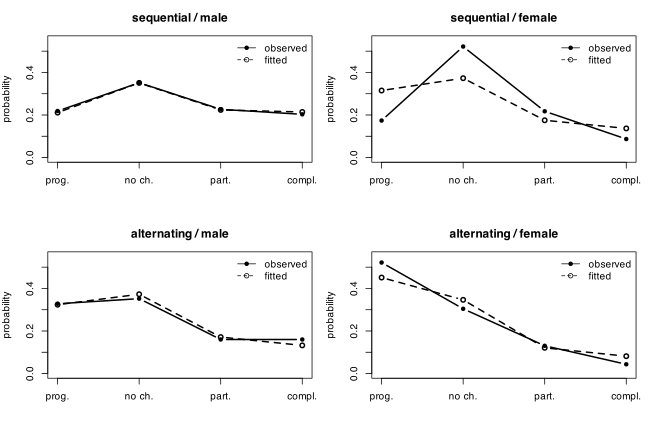
Part (c). The Wald statistic for \(H_0: \beta_1 = 0\) is \(b_1 / \mathrm{s.e.}(b_1) = -0.5807/0.2121 = -2.737\), or \(W = (b_1/\mathrm{s.e.}(b_1))^2 = 7.49\) compared with \(\chi^2(1)\).
z <- coef(summary(m))["treatmentalternating", "t value"]
c(z = z, W = z^2, p = pchisq(z^2, 1, lower.tail = FALSE))
z W p
-2.7371661 7.4920782 0.0061971
So \(p = 0.0062\): there is strong evidence of a treatment difference, sequential being better.
Part (d). Fit the proportional odds model with and without the treatment term and compare deviances, which is the likelihood ratio version of the same test.
m0 <- polr(response ~ sex, weights = frequency, data = tumor, Hess = TRUE)
anova(m0, m)
Likelihood ratio tests of ordinal regression models
Response: response
Model Resid. df Resid. Dev Test Df LR stat. Pr(Chi)
1 sex 295 796.6268
2 treatment + sex 294 789.0566 1 vs 2 1 7.570185 0.00593417
c(AIC.without = AIC(m0), AIC.with = AIC(m))
AIC.without AIC.with
804.6268 799.0566
The likelihood ratio statistic is \(\Delta D = 796.63 - 789.06 = 7.57\) on \(1\) df, \(p = 0.0059\), against the Wald \(W = 7.49\), \(p = 0.0062\). The two agree closely, as they must when the log-likelihood is nearly quadratic near the maximum and the sample is reasonably large: the Wald statistic is the quadratic approximation to the likelihood ratio statistic (Section 5.2). The likelihood ratio value is slightly the larger, which is the usual direction when the log-likelihood is a little flatter than quadratic on the side of the null value. AIC drops by \(5.6\) when treatment is included. Neither test is preferable on the evidence here; where they disagree the likelihood ratio statistic is generally to be trusted, since it is invariant to reparameterisation of \(\beta_1\) while the Wald statistic is not.
Part (e). Two preliminaries about what can actually be fitted. Model (8.16) as written models \(\log[\pi_j/(\pi_{j+1} + \ldots + \pi_J)]\), which is VGAM’s sratio family (its cratio family is the reciprocal, and would flip every sign). This is the model whose likelihood factorises: for each \(j\) the conditional distribution of “stop at \(j\)” given “reached \(j\)” is Binomial and the four multinomial cell counts split into three independent Binomials, so the model can be fitted equally well by three stacked binomial GLMs with any link, and different links may even be used for different \(j\). Model (8.15), by contrast, models \(\log(\pi_j/\pi_{j+1})\), which is an odds ranging over \((0, \infty)\), not a probability in \((0,1)\): probit and complementary log-log are simply not defined for it, and VGAM fails with NaNs produced in qnorm if asked. What can be done instead is to model the local conditional probability \(\pi_j/(\pi_j + \pi_{j+1})\) with those links, which coincides with (8.15) when the link is the logit. That fit is a pseudo-likelihood, because consecutive adjacent pairs share cell counts and are not independent, so its standard errors are not trustworthy; I report it with that caveat, together with the exact maximum likelihood adjacent-category fit under the log link.
The exact maximum likelihood fits, all with \(5\) parameters on the same \(16\) counts, so directly comparable by AIC. The proportional odds model of (a) is refitted here through VGAM so that it lands on the same log-likelihood scale as the rest: polr reports \(-394.53\) and vglm reports \(-25.54\), the difference being the constant multinomial coefficient \(\sum \log[n_i!/\prod_j y_{ij}!]\), which cancels in every comparison but has to be handled consistently.
library(VGAM)
w <- reshape(tumor, direction = "wide", idvar = c("treatment", "sex"),
timevar = "response", v.names = "frequency")
Y <- as.matrix(w[, 3:6]); colnames(Y) <- lev
fits <- list(
po.logit = vglm(Y ~ treatment + sex, cumulative(parallel = TRUE), data = w),
cr.logit = vglm(Y ~ treatment + sex, sratio(link = "logitlink", parallel = TRUE), data = w),
cr.probit = vglm(Y ~ treatment + sex, sratio(link = "probitlink", parallel = TRUE), data = w),
cr.cloglog = vglm(Y ~ treatment + sex, sratio(link = "clogloglink", parallel = TRUE), data = w),
acat.log = vglm(Y ~ treatment + sex, acat(reverse = TRUE, parallel = TRUE), data = w))
est <- sapply(fits, coef)
se <- sapply(fits, function(f) sqrt(diag(vcov(f))))
round(rbind(est, logLik = sapply(fits, logLik), AIC = sapply(fits, AIC)), 4)
po.logit cr.logit cr.probit cr.cloglog acat.log
(Intercept):1 -1.3180 -1.2184 -0.7507 -1.3097 -0.4577
(Intercept):2 0.2492 -0.2316 -0.1427 -0.5432 0.4558
(Intercept):3 1.3001 -0.0661 -0.0397 -0.4275 -0.0003
treatmentalternating 0.5807 0.3975 0.2457 0.2819 0.2889
sexfemale 0.5414 0.5355 0.3272 0.4153 0.3308
logLik -25.5417 -25.9874 -25.9597 -26.1737 -25.7347
AIC 61.0834 61.9748 61.9194 62.3474 61.4693
The first column is a useful check on part (a): vglm parameterises (8.14) exactly as the book does, with \(\pi_1 + \ldots + \pi_j\) in the numerator and \(+\mathbf{x}^T\boldsymbol{\beta}\) in the linear predictor, and it returns \(\beta_1 = 0.5807\), \(\beta_2 = 0.5414\) and \(\beta_{0j} = (-1.3180, 0.2492, 1.3001)\), which are the polr numbers with the sign flip undone.
round(se, 4)
po.logit cr.logit cr.probit cr.cloglog acat.log
(Intercept):1 0.1801 0.1650 0.0982 0.1351 0.1649
(Intercept):2 0.1621 0.1625 0.1009 0.1221 0.1736
(Intercept):3 0.1852 0.2100 0.1308 0.1504 0.1988
treatmentalternating 0.2119 0.1710 0.1046 0.1292 0.1148
sexfemale 0.2953 0.2437 0.1499 0.1739 0.1684
round(est / se, 3)
po.logit cr.logit cr.probit cr.cloglog acat.log
(Intercept):1 -7.319 -7.384 -7.647 -9.694 -2.776
(Intercept):2 1.538 -1.425 -1.414 -4.448 2.625
(Intercept):3 7.021 -0.315 -0.303 -2.841 -0.002
treatmentalternating 2.741 2.325 2.348 2.182 2.515
sexfemale 1.834 2.197 2.182 2.388 1.964
(The proportional odds standard errors differ from polr’s in the fourth decimal, \(0.2119\) against \(0.2121\), because vglm uses the expected information and polr a numerical Hessian; the Wald statistic is \(2.741\) either way.)
The stated factorisation is worth verifying, since it is what licenses fitting (8.16) by ordinary binomial GLMs:
cr <- do.call(rbind, lapply(1:3, function(j)
data.frame(w[, 1:2], cut = factor(j), y = Y[, j], n = rowSums(Y[, j:4, drop = FALSE]))))
g <- glm(cbind(y, n - y) ~ cut + treatment + sex, binomial("logit"), data = cr)
v <- vglm(Y ~ treatment + sex, sratio(link = "logitlink", parallel = TRUE), data = w)
rbind(stacked.glm = c(coef(g)[c("treatmentalternating", "sexfemale")],
logLik = as.numeric(logLik(g))),
vglm.sratio = c(coef(v)[c("treatmentalternating", "sexfemale")],
logLik = as.numeric(logLik(v))))
treatmentalternating sexfemale logLik
stacked.glm 0.3975226 0.5355538 -25.9874
vglm.sratio 0.3975245 0.5355499 -25.9874
The same device applied to overlapping adjacent pairs gives the pseudo-likelihood adjacent-category fits under the three links:
ad <- do.call(rbind, lapply(1:3, function(j)
data.frame(w[, 1:2], cut = factor(j), y = Y[, j], n = Y[, j] + Y[, j + 1])))
sapply(c("logit", "probit", "cloglog"), function(lk) {
g <- glm(cbind(y, n - y) ~ cut + treatment + sex, binomial(link = lk), data = ad)
round(coef(summary(g))[c("treatmentalternating", "sexfemale"), c(1, 2)], 4)
}, simplify = "array")
, , logit
Estimate Std. Error
treatmentalternating 0.3403 0.1926
sexfemale 0.2910 0.2654
, , probit
Estimate Std. Error
treatmentalternating 0.2105 0.1192
sexfemale 0.1801 0.1639
, , cloglog
Estimate Std. Error
treatmentalternating 0.2253 0.1315
sexfemale 0.2067 0.1750
How the different models affect the interpretation. Three things change and one does not.
What does not change is the conclusion. In every fit the alternating regime and female sex both push the response towards the bad end of the scale, and in every exact fit the treatment effect is significant at the \(5\%\) level: proportional odds \(|z| = 2.74\), continuation ratio \(2.32\) (logit), \(2.35\) (probit), \(2.18\) (cloglog), adjacent category \(2.52\) (the sign is \(-\) in the polr parameterisation and \(+\) in the book’s, and carries no extra information). The five models also fit about equally well: on the common vglm scale the AIC runs from \(61.08\) (proportional odds) through \(61.47\) (adjacent category), \(61.92\) and \(61.97\) (continuation ratio, probit and logit) to \(62.35\) (continuation ratio, complementary log-log), a spread of \(1.26\) over models with identical parameter counts on identical counts. Choosing among them is not a matter of fit.
What does change, first, is the scale on which the coefficient is an odds ratio, and hence what “the” treatment effect means. In the proportional odds model \(e^{0.5807} = 1.79\) is the odds ratio for the cumulative event “response no better than category \(j\)”, the same for every cutpoint. In the continuation ratio model \(e^{0.3975} = 1.49\) is the odds ratio for stopping at category \(j\) among patients who got at least that far, that is, a discrete hazard ratio, which is the natural quantity if one thinks of the patient as progressing through the categories in sequence. In the adjacent category model \(e^{0.2889} = 1.33\) is the odds ratio between two neighbouring categories only. The numbers differ by a factor of more than two, and quoting one as though it were another would be a serious misstatement.
Second, the link changes the numerical scale but not much else. Within the continuation ratio family, probit coefficients are \(0.62\) times the logit ones (\(0.2457\) against \(0.3975\)), and the fits are near-identical (\(\Delta\) logLik \(= 0.03\)). The factor is a scale change and nothing more: the standard logistic distribution has standard deviation \(\pi/\sqrt{3} = 1.81\) against \(1\) for the standard Normal, so matching the two on spread predicts a ratio of \(1/1.81 = 0.55\), while matching them where the data actually sit, near the middle of the distribution rather than in the tails, gives the familiar \(1/1.6\) to \(1/1.7\), that is \(0.59\) to \(0.62\). The observed \(0.62\) is in that range. Nothing in the interpretation depends on which of the two is used. The complementary log-log link fits marginally worse (\(\Delta\) logLik \(= 0.19\) against the logit) and, being asymmetric, has no odds ratio interpretation at all: \(e^{0.2819}\) is a ratio of complementary log-log transformed conditional probabilities, not an odds ratio, and the covariate effect is a proportional hazards effect on the underlying continuous scale. Section 8.5 makes this point: with \(z\) symmetric, logit and probit are appropriate and interchangeable; the complementary log-log link earns its place only when the latent distribution is markedly skewed, and here it is not.
Third, the pseudo-likelihood adjacent-category fits are visibly worse than the exact one and should not be quoted. Their logit coefficient for treatment is \(0.3403\) with standard error \(0.1926\), against \(0.2889\) with standard error \(0.1148\) from the exact fit; the treatment effect is no longer significant (\(p = 0.077\)) purely because the overlapping-pairs construction reuses each cell count twice and inflates the apparent uncertainty. I include them only because the exercise asks for probit and cloglog adjacent-category models, which do not exist in the form (8.15); the honest answer to that part of the question is that the adjacent-category model is defined on an odds scale, so the logit is the only one of the three links that applies to it, and confidence in the probit and cloglog numbers above is low.
Problem 8.4 — Consider ordinal response categories which can be interpreted in terms of
Consider ordinal response categories which can be interpreted in terms of continuous latent variable as shown in Figure 8.2. Suppose the distribution of this underlying variable is Normal. Show that the probit is the natural link function in this situation (Hint: See Section 7.3).
Figure 8.2 shows the density of a continuous latent variable \(z\) cut by three cutpoints \(C_1 < C_2 < C_3\) into four regions, whose areas are the category probabilities \(\pi_1, \pi_2, \pi_3, \pi_4\): \(\pi_1\) is the area to the left of \(C_1\), \(\pi_2\) the area between \(C_1\) and \(C_2\), \(\pi_3\) the area between \(C_2\) and \(C_3\), and \(\pi_4\) the area to the right of \(C_3\). (difficulty: \(\star\star\))
Set up the latent variable exactly as in Figure 8.2. For a subject with covariate vector \(\mathbf{x}\) let the unobserved variable be \(z \sim \mathrm{N}(\mu, \sigma^2)\), where the mean depends on the covariates through \(\mu = \mathbf{x}^T\boldsymbol{\beta}^{*}\) and \(\sigma\) does not. The cutpoints \(C_1 < C_2 < \ldots < C_{J-1}\) are fixed features of the measuring instrument, not of the subject, and the observed category is \(j\) when \(C_{j-1} < z \leqslant C_j\) (with \(C_0 = -\infty\), \(C_J = +\infty\)). So
\begin{equation*} \pi_j = P(C_{j-1} < z \leqslant C_j), \qquad \gamma_j \equiv \pi_1 + \ldots + \pi_j = P(z \leqslant C_j). \end{equation*}
Standardising,
\begin{equation*} \gamma_j = P\left(\frac{z - \mu}{\sigma} \leqslant \frac{C_j - \mu}{\sigma}\right) = \Phi\left(\frac{C_j - \mathbf{x}^T\boldsymbol{\beta}^{*}}{\sigma}\right), \end{equation*}
where \(\Phi\) is the standard Normal cumulative distribution function, as in Section 7.3. Applying \(\Phi^{-1}\) to both sides,
\begin{equation*} \Phi^{-1}(\gamma_j) = \frac{C_j}{\sigma} - \frac{\mathbf{x}^T\boldsymbol{\beta}^{*}}{\sigma} = \beta_{0j} - \mathbf{x}^T\boldsymbol{\beta}, \qquad \beta_{0j} = \frac{C_j}{\sigma}, \quad \boldsymbol{\beta} = \frac{\boldsymbol{\beta}^{*}}{\sigma}. \end{equation*}
This is exactly the structure of the proportional odds model (8.14), with \(\Phi^{-1}\) in place of the logit: a cutpoint-specific intercept plus a linear predictor that does not depend on \(j\). The minus sign is only a convention. The book writes (8.14) with \(+\beta_1 x_1 + \ldots\), which corresponds to replacing \(\boldsymbol{\beta}\) by \(-\boldsymbol{\beta}^{*}/\sigma\); keeping the minus sign, as polr does, makes a positive coefficient mean a push towards the high categories, which is the more readable convention when the latent variable is what one is thinking about. Three points follow, and together they are what “natural” means here.
First, \(\Phi^{-1}\) is the transformation that linearises. The cumulative probability \(\gamma_j\) is the latent cumulative distribution function evaluated at a linear function of \(\mathbf{x}\); the link that undoes the cumulative distribution function therefore returns a linear predictor, and no other link does. This is precisely the argument of Section 7.3, where a Uniform tolerance distribution gives the identity link, a logistic tolerance distribution gives the logit, and the Normal gives \(\Phi^{-1}(\pi) = \beta_1 + \beta_2 x\) with \(\beta_1 = -\mu/\sigma\) and \(\beta_2 = 1/\sigma\). Exercise 8.1 confirms the consistency of the two settings: with \(J = 2\) the display above collapses to \(\Phi^{-1}(\pi_1) = C_1/\sigma - \mathbf{x}^T\boldsymbol{\beta}^{*}/\sigma\), which is the binary probit model of Section 7.3 exactly.
Second, the proportional structure is not an extra assumption but a consequence. Because \(\sigma\) is the same for every category, the coefficient \(\boldsymbol{\beta}^{*}/\sigma\) is common to all \(J-1\) equations: the covariate shifts the whole latent distribution without changing its spread, so it shifts every cutpoint on the probit scale by the same amount. Model (8.14) requires this as an assumption (“wherever the cutpoints are, the odds ratio for a one unit change in \(x\) is the same”); the Normal latent variable with constant variance delivers it. If instead \(\sigma\) depended on \(\mathbf{x}\), the coefficient would become \(\boldsymbol{\beta}^{*}/\sigma(\mathbf{x})\) and the parallel structure would fail, for the probit as for the logit.
Third, the parameters are only identified up to the scale of \(z\), since \(C_j\) and \(\boldsymbol{\beta}^{*}\) enter only through \(C_j/\sigma\) and \(\boldsymbol{\beta}^{*}/\sigma\). Fixing \(\sigma = 1\) is the usual normalisation, and then \(\beta_{0j} = C_j\) and \(\boldsymbol{\beta} = \boldsymbol{\beta}^{*}\). Also, adding a constant to \(z\) and to every \(C_j\) changes nothing, which is why the linear predictor carries no separate intercept.
One qualification, since the word “natural” is used in two different senses in this book. The probit is not the canonical link in the exponential family sense of Section 3.3: for Binomial data the canonical link is the logit, and \(\Phi^{-1}\) is not of the form \({b^{\prime}}^{-1}\) for any exponential family representation used here. What has been shown is that \(\Phi^{-1}\) is the link naturally induced by the Normal latent (tolerance) distribution, which is the sense of Section 7.3 and the sense the exercise’s hint points at. Section 8.5 makes the same distinction from the other side: the optimal link depends on the shape of the distribution of \(z\), with logits and probits appropriate for symmetric latent distributions and complementary log-log better for skewed ones.
A simulation confirms the algebra: generate a latent Normal with known \(\sigma\), \(\boldsymbol{\beta}^{*}\) and cutpoints, discretise it, and check that the cumulative probit model recovers \(C_j/\sigma\) and \(\beta^{*}/\sigma\).
library(MASS)
set.seed(20260831)
n <- 200000
x <- rbinom(n, 1, 0.5)
beta.star <- 1.2; sigma <- 2; C <- c(-1, 0.5, 2.5)
z <- rnorm(n, mean = beta.star * x, sd = sigma)
y <- ordered(cut(z, breaks = c(-Inf, C, Inf), labels = 1:4))
fit <- polr(y ~ x, method = "probit")
round(rbind(fitted = c(fit$zeta, x = coef(fit)),
theory = c(C / sigma, x = beta.star / sigma)), 4)
1|2 2|3 3|4 x.x
fitted -0.4971 0.252 1.255 0.6008
theory -0.5000 0.250 1.250 0.6000
The estimates match \(C_j/\sigma = (-0.5, 0.25, 1.25)\) and \(\beta^{*}/\sigma = 0.6\) to within Monte Carlo error, and note that neither \(\sigma\) nor the raw \(C_j\) are separately recoverable, as the identifiability remark predicts.
Poisson Regression and Log-Linear Models
Problem 9.1 — Let Y1 , . . . ,YN be independent random variables with Yi \(\sim\) Po(µi ) and
Let \(Y_1, \ldots, Y_N\) be independent random variables with \(Y_i \sim \mathrm{Po}(\mu_i)\) and
\begin{equation*} \log \mu_i = \beta_1 + \sum_{j=2}^{J} x_{ij}\beta_j, \qquad i = 1, \ldots, N . \end{equation*}
a. Show that the score statistic for \(\beta_1\) is \(U_1 = \sum_{i=1}^{N}(Y_i - \mu_i)\).
b. Hence, show that for maximum likelihood estimates \(\widehat{\mu}_i\), \(\sum \widehat{\mu}_i = \sum y_i\).
c. Deduce that the expression for the deviance in (9.6) simplifies to (9.7) in this case. (difficulty: \(\star\))
Write the linear predictor as \(\eta_i = \mathbf{x}_i^T\boldsymbol{\beta}\) with \(\mathbf{x}_i = (1, x_{i2}, \ldots, x_{iJ})^T\); the leading \(1\) is what makes \(\beta_1\) an intercept, and it is the only feature of the model used below.
(a) The score for the intercept.
The Poisson probability function is \(f(y_i; \mu_i) = \mu_i^{y_i}e^{-\mu_i}/y_i!\), so the log-likelihood is
\begin{equation*} \ell(\boldsymbol{\beta}; \mathbf{y}) = \sum_{i=1}^{N}\left[ y_i \log \mu_i - \mu_i - \log y_i! \right]. \end{equation*}
Since \(\log \mu_i = \mathbf{x}_i^T\boldsymbol{\beta}\) we have \(\mu_i = \exp(\mathbf{x}_i^T\boldsymbol{\beta})\) and hence \(\partial \mu_i / \partial \beta_j = \mu_i x_{ij}\). Differentiating term by term,
\begin{equation*} U_j = \frac{\partial \ell}{\partial \beta_j} = \sum_{i=1}^{N}\left[\frac{y_i}{\mu_i} - 1\right]\frac{\partial \mu_i}{\partial \beta_j} = \sum_{i=1}^{N}\left[\frac{y_i}{\mu_i} - 1\right]\mu_i x_{ij} = \sum_{i=1}^{N}(y_i - \mu_i)\,x_{ij}, \qquad j = 1, \ldots, J . \end{equation*}
This is the general Poisson score vector; it is the specialisation of the score in Section 4.3 to the log link, for which the link is canonical and the weights cancel. Putting \(j = 1\) and \(x_{i1} = 1\) for every \(i\),
\begin{equation*} U_1 = \sum_{i=1}^{N}(Y_i - \mu_i), \end{equation*}
as required. Note \(\mathrm{E}(U_1) = 0\) because \(\mathrm{E}(Y_i) = \mu_i\), as it must be for a score statistic.
(b) The fitted values sum to the data total.
The maximum likelihood estimates \(\mathbf{b}\) solve \(U_j = 0\) simultaneously for \(j = 1, \ldots, J\). The first of these equations, evaluated at \(\mathbf{b}\), gives
\begin{equation*} 0 = U_1(\mathbf{b}) = \sum_{i=1}^{N}\left(y_i - \widehat{\mu}_i\right) \qquad\Longrightarrow\qquad \sum_{i=1}^{N}\widehat{\mu}_i = \sum_{i=1}^{N} y_i , \end{equation*}
where \(\widehat{\mu}_i = \exp(\mathbf{x}_i^T\mathbf{b})\). In the notation of Section 9.2, \(\sum e_i = \sum o_i\): the fitted (expected) frequencies reproduce the grand total exactly. The only thing that was used is that the model contains a constant term, so this holds for essentially every Poisson model in the chapter, including all the log-linear models of Section 9.5, whose minimal model \(\log \mathrm{E}(Y_{jk}) = \mu\) already contains the constant. It fails only for a model fitted without an intercept, or without any set of indicator variables that sums to a column of ones.
(c) The deviance.
The deviance for a Poisson model, equation (9.6), is
\begin{equation*} D = 2\sum_{i=1}^{N}\left[o_i \log\!\left(\frac{o_i}{e_i}\right) - (o_i - e_i)\right]. \end{equation*}
By part (b) the second group of terms sums to zero,
\begin{equation*} \sum_{i=1}^{N}(o_i - e_i) = \sum y_i - \sum \widehat{\mu}_i = 0, \end{equation*}
so the whole correction disappears and
\begin{equation*} D = 2\sum_{i=1}^{N} o_i \log\!\left(\frac{o_i}{e_i}\right), \end{equation*}
which is equation (9.7). This is exactly the form of the likelihood ratio chi-squared statistic \(G^2\) familiar from contingency tables. It is worth stressing that the two expressions agree only because of the intercept: (9.6) is the correct deviance in general and (9.7) is a convenience that the intercept buys. (9.6) is also the expression that guarantees \(D \geqslant 0\) term by term, since each summand is \(2e_i\,h(o_i/e_i)\) with \(h(t) = t\log t - t + 1 \geqslant 0\); the summands of (9.7) can individually be negative even though their total is not.
Numerical check. The British doctors data of Section 9.2.1, fitted with Model (9.9), lets us confirm all three parts at once, and a deliberately intercept-free model shows what happens when the hypothesis of part (b) is dropped.
library(dobson)
data(doctors)
d <- doctors
d$agecat <- rep(1:5, 2)
d$agesq <- d$agecat^2
d$smoke <- as.numeric(d$smoking == "smoker")
d$smkage <- d$smoke * d$agecat
# 'poisson' is a dobson data set, so the family function needs its namespace
fit <- glm(deaths ~ smoke + agecat + agesq + smkage +
offset(log(`person-years`)), family = stats::poisson, data = d)
o <- d$deaths; e <- fitted(fit)
cat("sum(o) =", sum(o), " sum(e) =", sum(e), "\n")
cat("score for beta1 = sum(o - e) =", sum(o - e), "\n")
cat("D from (9.6) =", 2 * sum(o * log(o / e) - (o - e)),
" D from (9.7) =", 2 * sum(o * log(o / e)),
" deviance(fit) =", deviance(fit), "\n")
fit0 <- glm(deaths ~ 0 + agecat + offset(log(`person-years`)),
family = stats::poisson, data = d)
e0 <- fitted(fit0)
cat("no intercept: sum(o - e) =", sum(o - e0),
" (9.6) =", 2 * sum(o * log(o / e0) - (o - e0)),
" (9.7) =", 2 * sum(o * log(o / e0)), "\n")
sum(o) = 731 sum(e) = 731
score for beta1 = sum(o - e) = 9.361401e-13
D from (9.6) = 1.63537 D from (9.7) = 1.63537 deviance(fit) = 1.63537
no intercept: sum(o - e) = -1695.874 (9.6) = 13211 (9.7) = 9819.252
The intercept model reproduces the grand total \(731\) to numerical precision and the two deviance formulae agree at \(D = 1.635\), the value quoted in Table 9.3. Removing the intercept breaks \(\sum o_i = \sum e_i\), and (9.6) then exceeds (9.7) by exactly \(-2\sum(o_i - e_i) = 3391.75\); only (9.6) equals deviance().
Problem 9.2 — The data in Table 9.13 are numbers of insurance policies, n, and numbers
The data in Table 9.13 are numbers of insurance policies, \(n\), and numbers of claims, \(y\), for cars in various insurance categories, CAR, tabulated by age of policy holder, AGE, and district where the policy holder lived (DIST \(= 1\), for London and other major cities, and DIST \(= 0\), otherwise). The table is derived from the CLAIMS data set in Aitkin et al. (2005) obtained from a paper by Baxter et al. (1980).
a. Calculate the rate of claims \(y/n\) for each category and plot the rates by AGE, CAR and DIST to get an idea of the main effects of these factors.
b. Use Poisson regression to estimate the main effects (each treated as categorical and modelled using indicator variables) and interaction terms.
c. Based on the modelling in (b), Aitkin et al. (2005) determined that all the interactions were unimportant and decided that AGE and CAR could be treated as though they were continuous variables. Fit a model incorporating these features and compare it with the best model obtained in (b). What conclusions do you reach?
Table 9.13 (car insurance claims) gives, for each combination of CAR \(= 1,2,3,4\) and AGE \(= 1,2,3,4\), the pair \((y, n)\) separately for DIST \(= 0\) and DIST \(= 1\). For DIST \(= 0\) the sixteen pairs, in the order CAR \(=1\) with AGE \(=1,\ldots,4\), then CAR \(=2\) with AGE \(=1,\ldots,4\), and so on, are \((65, 317)\), \((65, 476)\), \((52, 486)\), \((310, 3259)\); \((98, 486)\), \((159, 1004)\), \((175, 1355)\), \((877, 7660)\); \((41, 223)\), \((117, 539)\), \((137, 697)\), \((477, 3442)\); \((11, 40)\), \((35, 148)\), \((39, 214)\), \((167, 1019)\). For DIST \(= 1\), in the same order, they are \((2, 20)\), \((5, 33)\), \((4, 40)\), \((36, 316)\); \((7, 31)\), \((10, 81)\), \((22, 122)\), \((102, 724)\); \((5, 18)\), \((7, 39)\), \((16, 68)\), \((63, 344)\); \((0, 3)\), \((6, 16)\), \((8, 25)\), \((33, 114)\). (difficulty: \(\star\star\star\))
The response is a count of claims \(Y_i\) out of a known number of policies \(n_i\), so this is the rate model of Section 9.2: \(Y_i \sim \mathrm{Po}(\mu_i)\) with \(\mu_i = n_i\theta_i\) and, by equation (9.3),
\begin{equation*} \log \mu_i = \log n_i + \mathbf{x}_i^T\boldsymbol{\beta}, \end{equation*}
the offset \(\log n_i\) carrying the exposure. Parameters are interpreted as rate ratios \(e^{\beta_j}\). The data ship as insurance in the dobson package.
(a) Observed rates.
library(dobson)
data(insurance)
ins <- insurance
ins$rate <- 1000 * ins$y / ins$n
print(round(xtabs(rate ~ car + age + district, data = ins), 1))
mg <- function(v) round(1000 * tapply(ins$y, ins[[v]], sum) / tapply(ins$n, ins[[v]], sum), 1)
rbind(CAR = mg("car"), AGE = mg("age"))
mg("district")
, , district = 0
age
car 1 2 3 4
1 205.0 136.6 107.0 95.1
2 201.6 158.4 129.2 114.5
3 183.9 217.1 196.6 138.6
4 275.0 236.5 182.2 163.9
, , district = 1
age
car 1 2 3 4
1 100.0 151.5 100.0 113.9
2 225.8 123.5 180.3 140.9
3 277.8 179.5 235.3 183.1
4 0.0 375.0 320.0 289.5
1 2 3 4
CAR 109.0 126.5 160.7 189.4
AGE 201.2 172.9 150.6 122.3
0 1
132.2 163.5
Rates are claims per 1000 policies per year. The marginal patterns are clean and monotone: the rate rises steadily with CAR (109 to 189 per 1000 from category 1 to 4) and falls steadily with AGE (201 down to 122), and it is about a quarter higher in the major cities (163.5 against 132.2).
op <- par(mfrow = c(1, 2), mar = c(4.5, 4.5, 3, 1))
for (dd in 0:1) {
s <- ins[ins$district == dd, ]
plot(range(s$age), range(ins$rate), type = "n", xlab = "AGE group",
ylab = "claims per 1000 policies", xaxt = "n",
main = paste0("DIST = ", dd, if (dd == 1) " (major cities)" else " (elsewhere)"))
axis(1, at = 1:4)
for (cc in 1:4) {
z <- s[s$car == cc, ]
lines(z$age, z$rate, type = "b", pch = 14 + cc, lty = cc, col = cc + 1, lwd = 2)
}
if (dd == 0) legend("topright", legend = paste("CAR", 1:4), pch = 15:18,
lty = 1:4, col = 2:5, bty = "n", lwd = 2)
}
par(op)
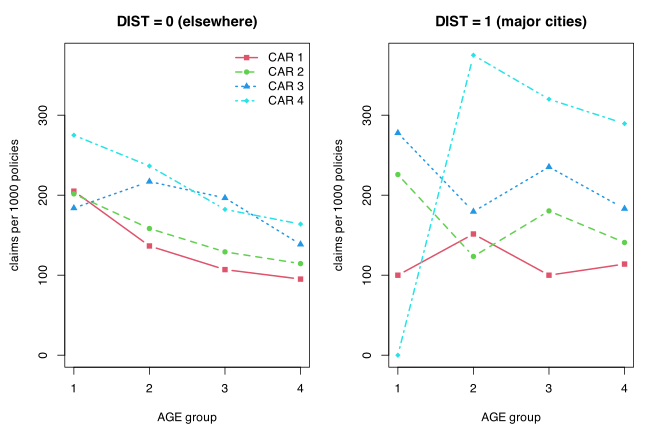
In the left panel (DIST \(= 0\), where nearly all the exposure lies) the four CAR curves are stacked in order and fall with AGE at much the same rate, which is what an additive model on the log scale predicts: no interaction. The only visible departure is CAR \(=3\) rising from AGE \(=1\) to AGE \(=2\), and part (b) shows it is well within sampling error. The right panel is much noisier because those cells contain very few policies – CAR \(= 4\), AGE \(= 1\) has \(n = 3\) and \(y = 0\), and the visually dramatic jump from 0 to 375 per 1000 rests on three policies. Sampling noise, not an interaction, is the natural reading.
(b) Poisson regression with categorical effects.
ins$CAR <- factor(ins$car); ins$AGE <- factor(ins$age); ins$DIST <- factor(ins$district)
P <- function(f) glm(f, family = stats::poisson, data = ins, offset = log(n))
m0 <- P(y ~ 1); m1 <- P(y ~ CAR + AGE + DIST)
m2 <- P(y ~ CAR + AGE + DIST + CAR:AGE)
m3 <- P(y ~ CAR + AGE + DIST + CAR:DIST)
m4 <- P(y ~ CAR + AGE + DIST + AGE:DIST)
m5 <- P(y ~ (CAR + AGE + DIST)^2); m6 <- P(y ~ CAR * AGE * DIST)
ms <- list(m0, m1, m2, m3, m4, m5, m6)
data.frame(model = c("minimal", "main effects", "+ CAR:AGE", "+ CAR:DIST",
"+ AGE:DIST", "all two-way", "saturated"),
df = sapply(ms, df.residual),
deviance = round(sapply(ms, deviance), 3),
AIC = round(sapply(ms, AIC), 1))
model df deviance AIC
1 minimal 31 207.833 378.2
2 main effects 24 23.709 208.1
3 + CAR:AGE 15 13.192 215.6
4 + CAR:DIST 21 19.272 209.6
5 + AGE:DIST 21 19.920 210.3
6 all two-way 9 5.295 219.7
7 saturated 0 0.000 232.4
The three main effects between them take the deviance from \(207.8\) on 31 d.f. to \(23.7\) on 24 d.f., a drop of \(184.1\) on 7 d.f. – overwhelming. The main-effects model already fits: \(D = 23.71\) on 24 d.f. gives \(p = 0.48\) against \(\chi^2(24)\). None of the interactions is needed:
rbind("CAR:AGE" = unlist(anova(m1, m2, test = "Chisq")[2, c("Df", "Deviance", "Pr(>Chi)")]),
"CAR:DIST" = unlist(anova(m1, m3, test = "Chisq")[2, c("Df", "Deviance", "Pr(>Chi)")]),
"AGE:DIST" = unlist(anova(m1, m4, test = "Chisq")[2, c("Df", "Deviance", "Pr(>Chi)")]))
Df Deviance Pr(>Chi)
CAR:AGE 9 10.517305 0.3102500
CAR:DIST 3 4.437058 0.2179738
AGE:DIST 3 3.789357 0.2851265
Each interaction costs a lot of parameters and buys almost nothing, and AIC rises for every one of them. So the best model in (b) is the main-effects model:
summary(m1)
Coefficients:
Estimate Std. Error z value Pr(>|z|)
(Intercept) -1.81021 0.07532 -24.034 < 2e-16 ***
CAR2 0.16229 0.05052 3.213 0.001315 **
CAR3 0.39352 0.05498 7.157 8.25e-13 ***
CAR4 0.56540 0.07228 7.823 5.18e-15 ***
AGE2 -0.18902 0.08282 -2.282 0.022477 *
AGE3 -0.34211 0.08130 -4.208 2.58e-05 ***
AGE4 -0.53275 0.06979 -7.634 2.28e-14 ***
DIST1 0.21850 0.05853 3.733 0.000189 ***
Null deviance: 207.833 on 31 degrees of freedom
Residual deviance: 23.709 on 24 degrees of freedom
AIC: 208.07
Relative to CAR \(=1\), AGE \(=1\), DIST \(=0\), the estimated rate ratios are \(e^{0.162} = 1.18\), \(e^{0.394} = 1.48\), \(e^{0.565} = 1.76\) across CAR categories and \(e^{-0.189} = 0.83\), \(e^{-0.342} = 0.71\), \(e^{-0.533} = 0.59\) across AGE groups, with \(e^{0.219} = 1.24\) for city residence. Both sets of contrasts are monotone and, crucially, close to equally spaced on the log scale: the CAR steps are \(0.162, 0.231, 0.172\) and the AGE steps are \(-0.189, -0.153, -0.191\). That regularity is the empirical fact behind part (c).
(c) AGE and CAR as continuous.
Equal spacing of the log-scale contrasts is exactly what a linear term in the coded level \(1,2,3,4\) imposes, so replacing the two factors by the scores themselves should cost nothing.
mc <- glm(y ~ car + age + DIST, family = stats::poisson, data = ins, offset = log(n))
summary(mc)
round(exp(cbind(estimate = coef(mc), confint.default(mc))), 3)
Coefficients:
Estimate Std. Error z value Pr(>|z|)
(Intercept) -1.85253 0.07990 -23.185 < 2e-16 ***
car 0.19777 0.02080 9.507 < 2e-16 ***
age -0.17674 0.01849 -9.559 < 2e-16 ***
DIST1 0.21865 0.05853 3.736 0.000187 ***
Null deviance: 207.833 on 31 degrees of freedom
Residual deviance: 24.685 on 28 degrees of freedom
AIC: 201.05
estimate 2.5 % 97.5 %
(Intercept) 0.157 0.134 0.183
car 1.219 1.170 1.269
age 0.838 0.808 0.869
DIST1 1.244 1.110 1.396
anova(mc, m1, test = "Chisq")
c(AIC.continuous = AIC(mc), AIC.categorical = AIC(m1))
X2 <- sum(residuals(mc, "pearson")^2)
c(X2 = X2, df = df.residual(mc), p = pchisq(X2, df.residual(mc), lower.tail = FALSE))
Analysis of Deviance Table
Model 1: y ~ car + age + DIST
Model 2: y ~ CAR + AGE + DIST
Resid. Df Resid. Dev Df Deviance Pr(>Chi)
1 28 24.685
2 24 23.709 4 0.97633 0.9134
AIC.continuous AIC.categorical
201.0456 208.0693
X2 df p
23.497605 28.000000 0.707754
Collapsing six indicator parameters to two slopes costs a deviance of only \(0.98\) on 4 d.f. (\(p = 0.91\)) – the linearity restriction is entirely consistent with the data. The continuous model has \(D = 24.69\) and \(X^2 = 23.50\) on 28 d.f. (\(p = 0.71\)), so it fits the 32 cells well in absolute terms, and its AIC is 7 points lower than the categorical model’s. It is the model to report.
r <- rstandard(mc); o <- order(-abs(r))[1:4]
round(cbind(ins[o, c("car", "age", "district", "y", "n")],
fitted = fitted(mc)[o], rstd = r[o]), 2)
car age district y n fitted rstd
1 1 1 0 65 317 50.77 2.07
11 3 3 0 137 697 116.44 1.92
9 3 1 0 41 223 53.05 -1.85
32 4 4 1 33 114 24.20 1.79
No standardised residual exceeds \(2.1\) in absolute value on 32 cells, so there is no cell the model badly misses – in particular the eye-catching DIST \(= 1\) cells with tiny \(n\) are not outliers once their small exposure is accounted for.
Conclusions. Claim rates depend on all three factors and on none of their interactions, so the effects are multiplicative and act independently. Each one-step rise in insurance category CAR multiplies the claim rate by \(1.22\) (95% CI \(1.17\) to \(1.27\)); each one-step rise in the AGE band multiplies it by \(0.84\) (\(0.81\) to \(0.87\)), so the oldest band has \(0.84^3 = 0.59\) the rate of the youngest; and living in London or another major city multiplies it by \(1.24\) (\(1.11\) to \(1.40\)). Because there is no interaction, the city loading of about 24% applies uniformly to every CAR by AGE cell, and the CAR and AGE gradients are the same inside and outside the cities. Interpreting the CAR and AGE slopes literally does assume the four levels of each are equally spaced on some underlying scale, which the book’s coding gives no direct evidence for; the justification here is purely empirical, namely that the fitted categorical contrasts turned out to be equally spaced, which is what the test in the table above confirms.
Problem 9.3 — This question relates to the flu vaccine trial data in Table 9.6.
This question relates to the flu vaccine trial data in Table 9.6.
a. Using a conventional chi-squared test and an appropriate log-linear model, test the hypothesis that the distribution of responses is the same for the placebo and vaccine groups.
b. For the model corresponding to the hypothesis of homogeneity of response distributions, calculate the fitted values, the Pearson and deviance residuals, and the goodness of fit statistics \(X^2\) and \(D\). Which of the cells of the table contribute most to \(X^2\) (or \(D\))? Explain and interpret these results.
c. Re-analyze these data using ordinal logistic regression to estimate cutpoints for a latent continuous response variable and to estimate a location shift between the two treatment groups. Sketch a rough diagram to illustrate the model which forms the conceptual base for this analysis (see Exercise 8.4).
Table 9.6 (flu vaccine trial) is a \(2\times 3\) table of frequencies. The rows are the treatment groups and the columns are the response categories small, moderate and large. The placebo row is \(25\), \(8\), \(5\) with row total \(38\); the vaccine row is \(6\), \(18\), \(11\) with row total \(35\). (difficulty: \(\star\star\))
These are the data of Example 9.3.2: a randomized trial in which patients were allocated to vaccine or placebo and their haemagglutinin inhibiting antibody titre six weeks later was graded small, moderate or large. The row totals \(38\) and \(35\) are fixed by the design, so the joint distribution is product multinomial and, following Section 9.5, the minimal log-linear model must contain \(\alpha_j\):
\begin{equation*} \log \mathrm{E}(Y_{jk}) = \mu + \alpha_j . \end{equation*}
Homogeneity of the response distributions is \(\theta_{jk} = \theta_{\cdot k}\) for all \(j\), that is, the additive model \(\mu + \alpha_j + \beta_k\); the alternative is the saturated model \(\mu + \alpha_j + \beta_k + (\alpha\beta)_{jk}\).
(a) Chi-squared test and log-linear model.
library(dobson)
data(vaccine)
v <- vaccine
v$response <- factor(v$response, levels = c("small", "moderate", "large"))
tab <- xtabs(frequency ~ treatment + response, data = v)
tab
chisq.test(tab)
response
treatment small moderate large
placebo 25 8 5
vaccine 6 18 11
Pearson's Chi-squared test
data: tab
X-squared = 17.648, df = 2, p-value = 0.0001472
sat <- glm(frequency ~ treatment * response, family = stats::poisson, data = v)
add <- glm(frequency ~ treatment + response, family = stats::poisson, data = v)
anova(add, sat, test = "Chisq")
Analysis of Deviance Table
Model 1: frequency ~ treatment + response
Model 2: frequency ~ treatment * response
Resid. Df Resid. Dev Df Deviance Pr(>Chi)
1 2 18.642
2 0 0.000 2 18.642 8.95e-05 ***
The two analyses agree, as they must by Section 9.7.1: the conventional statistic \(X^2 = 17.65\) on 2 d.f. (\(p = 0.00015\)) and the deviance difference \(\Delta D = 18.64\) on 2 d.f. (\(p = 0.00009\)) are the Pearson and likelihood ratio versions of the same test of the same null hypothesis. The interaction terms \((\alpha\beta)_{jk}\) are needed: the distribution of responses is not the same in the two groups.
(b) Fitted values and residuals under homogeneity.
data.frame(v[, c("treatment", "response")], observed = v$frequency,
fitted = round(fitted(add), 3),
pearson = round(residuals(add, "pearson"), 3),
deviance = round(residuals(add, "deviance"), 3))
X2 <- sum(residuals(add, "pearson")^2); D <- deviance(add)
c(X2 = X2, D = D, df = df.residual(add),
p.X2 = pchisq(X2, df.residual(add), lower.tail = FALSE),
p.D = pchisq(D, df.residual(add), lower.tail = FALSE))
round(residuals(add, "pearson")^2, 3)
treatment response observed fitted pearson deviance
placebo small 25 16.137 2.206 2.040
placebo moderate 8 13.534 -1.504 -1.630
placebo large 5 8.329 -1.153 -1.247
vaccine small 6 14.863 -2.299 -2.615
vaccine moderate 18 12.466 1.567 1.469
vaccine large 11 7.671 1.202 1.128
X2 D df p.X2 p.D
1.764783e+01 1.864253e+01 2.000000e+00 1.471709e-04 8.950070e-05
1 2 3 4 5 6
4.868 2.263 1.330 5.285 2.457 1.444
The fitted values are the usual \(e_{jk} = y_{j\cdot}y_{\cdot k}/n\): for example \(38 \times 31/73 = 16.14\). They reproduce the fixed row totals exactly (\(16.137 + 13.534 + 8.329 = 38\)), which is the content of Exercise 9.1(b) applied to a model containing \(\alpha_j\). The goodness of fit statistics of the additive model, \(X^2 = 17.65\) and \(D = 18.64\) on 2 d.f., are the same numbers as in (a), because with a \(2\times 3\) table the saturated alternative has zero deviance.
The two “small” cells dominate: they contribute \(4.87 + 5.29 = 10.15\) of the \(17.65\), that is 58% of \(X^2\), and their deviance residuals (\(2.04\) and \(-2.62\)) are the two largest in magnitude. The pattern is a clean monotone gradient. Under homogeneity the placebo group should have produced about 16 small responses and produced 25; the vaccine group should have produced about 15 and produced 6. The signs then reverse for moderate and again stay reversed for large. So the vaccine group is shifted away from small titres and towards moderate and large ones. Reading the row percentages, small/moderate/large is \(66/21/13\) per cent under placebo and \(17/51/31\) per cent under vaccine. That is the clinically relevant conclusion: the vaccine raises the antibody response.
Because the discrepancies are monotone in an ordered response, the \(2\) d.f. chi-squared test is wasting power. That is what part (c) fixes.
(c) Ordinal logistic regression.
The conceptual base (Exercise 8.4, Section 8.3.3) is a latent continuous antibody response \(z\) which is not observed; instead it is recorded as small, moderate or large according to whether \(z\) falls below \(C_1\), between \(C_1\) and \(C_2\), or above \(C_2\). Treatment shifts the whole latent distribution by an amount \(\beta\) without changing its shape, and \(z\) is taken to have a logistic distribution. This gives the proportional odds model
\begin{equation*} \log\left(\frac{\Pr(Y \leqslant j)}{1 - \Pr(Y \leqslant j)}\right) = C_j - \beta\,x , \qquad j = 1, 2 , \end{equation*}
with \(x = 1\) for vaccine and \(0\) for placebo. Two cutpoints plus one shift is 3 parameters for 4 free cell probabilities, so there is 1 d.f. left to test the fit.
suppressMessages(library(MASS)) # note: MASS masks the dobson 'housing' data set
v$response <- factor(v$response, levels = c("small", "moderate", "large"), ordered = TRUE)
v$treatment <- factor(v$treatment, levels = c("placebo", "vaccine"))
po <- polr(response ~ treatment, weights = frequency, data = v, Hess = TRUE)
summary(po)
round(exp(c(OR = coef(po), confint.default(po))), 3)
Coefficients:
Value Std. Error t value
treatmentvaccine 1.838 0.4882 3.764
Intercepts:
Value Std. Error t value
small|moderate 0.5654 0.3434 1.6465
moderate|large 2.4414 0.4525 5.3948
Residual Deviance: 139.6736
AIC: 145.6736
OR.treatmentvaccine
6.283 2.413 16.357
The estimated cutpoints on the latent logistic scale are \(\widehat{C}_1 = 0.565\) and \(\widehat{C}_2 = 2.441\), and the estimated location shift is \(\widehat{\beta} = 1.838\) with standard error \(0.488\). The shift is \(3.76\) standard errors from zero. On the odds scale the vaccine multiplies the odds of a higher response category by \(e^{1.838} = 6.3\) (95% CI \(2.4\) to \(16.4\)), and by the proportional odds assumption that single ratio applies both to “moderate or large versus small” and to “large versus small or moderate”.
po0 <- polr(response ~ 1, weights = frequency, data = v, Hess = TRUE)
c(dev.diff = deviance(po0) - deviance(po),
p = pchisq(deviance(po0) - deviance(po), 1, lower.tail = FALSE))
pr <- predict(po, newdata = data.frame(treatment = factor(c("placebo", "vaccine"))),
type = "probs")
rownames(pr) <- c("placebo", "vaccine")
round(pr, 3)
round(pr * c(38, 35), 2)
obs <- as.vector(t(tab)); ex <- as.vector(t(pr * c(38, 35)))
c(X2 = sum((obs - ex)^2 / ex), D = 2 * sum(obs * log(obs / ex)), df = 1)
dev.diff p
1.568242e+01 7.491725e-05
small moderate large
placebo 0.638 0.282 0.080
vaccine 0.219 0.428 0.354
small moderate large
placebo 24.23 10.72 3.04
vaccine 7.66 14.97 12.37
X2 D df
3.102269 2.960108 1.000000
The likelihood ratio test for the shift is \(15.68\) on 1 d.f. (\(p = 7.5\times 10^{-5}\)), against \(18.64\) on 2 d.f. from the log-linear analysis. The ordinal model spends one degree of freedom instead of two and recovers almost all of the signal, which is the gain from using the ordering. The proportional odds restriction itself is acceptable: the fitted counts leave \(X^2 = 3.10\) and \(D = 2.96\) on 1 d.f. (\(p \approx 0.08\)), so the model is a fair, if not perfect, description – the residual lack of fit is in the same “small” cells, whose fitted counts \(24.2\) and \(7.7\) still slightly understate the separation between the groups.
C1 <- 0.5654; C2 <- 2.4414; shift <- 1.838
z <- seq(-5, 8, length = 800)
plot(z, dlogis(z), type = "l", lwd = 2, col = "grey30", ylim = c(0, 0.30),
xlab = "latent antibody response z", ylab = "density",
main = "Latent continuous response with fixed cutpoints and a location shift")
lines(z, dlogis(z, location = shift), lwd = 2, col = "firebrick", lty = 2)
abline(v = c(C1, C2), lty = 3, lwd = 2)
text(c(C1, C2), 0.295, c(expression(C[1]), expression(C[2])), pos = 4)
text(-2.6, 0.27, "placebo", col = "grey30", font = 2)
text(4.6, 0.27, "vaccine", col = "firebrick", font = 2)
arrows(0, 0.245, shift, 0.245, code = 3, length = 0.10, lwd = 2, col = "firebrick")
text(shift/2, 0.258, expression(beta == 1.84), col = "firebrick")
text(c(-2.0, 1.5, 5.0), 0.02, c("small", "moderate", "large"), cex = 1.05)
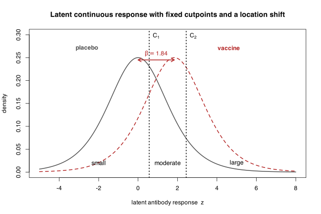
The diagram makes the model’s content plain. One latent density, drawn twice: solid for placebo, centred at \(0\), and dashed for vaccine, the identical curve slid \(1.84\) units to the right. The two vertical cutpoints \(C_1\) and \(C_2\) do not move, and the areas they cut off from each curve are the response probabilities \(0.638, 0.282, 0.080\) and \(0.219, 0.428, 0.354\). Sliding the curve right moves probability mass out of the “small” region and into “large”, which is precisely the pattern the residuals in part (b) were pointing at.
Problem 9.4 — For a 2× 2 contingency table, the maximal log-linear model can be written
For a \(2\times 2\) contingency table, the maximal log-linear model can be written as
\begin{equation*} \eta_{11} = \mu + \alpha + \beta + (\alpha\beta), \qquad \eta_{12} = \mu + \alpha - \beta - (\alpha\beta), \end{equation*}
\begin{equation*} \eta_{21} = \mu - \alpha + \beta - (\alpha\beta), \qquad \eta_{22} = \mu - \alpha - \beta + (\alpha\beta), \end{equation*}
where \(\eta_{jk} = \log \mathrm{E}(Y_{jk}) = \log(n\theta_{jk})\) and \(n = \sum\sum Y_{jk}\).
Show that the interaction term \((\alpha\beta)\) is given by
\begin{equation*} (\alpha\beta) = \tfrac{1}{4}\log\phi , \end{equation*}
where \(\phi\) is the odds ratio \((\theta_{11}\theta_{22})/(\theta_{12}\theta_{21})\), and hence that \(\phi = 1\) corresponds to no interaction. (difficulty: \(\star\))
This is the sum-to-zero parametrisation of the saturated model \(\log \mathrm{E}(Y_{jk}) = \mu + \alpha_j + \beta_k + (\alpha\beta)_{jk}\) of Section 9.5, with the constraints written into the four equations: \(\alpha_1 = -\alpha_2 = \alpha\), \(\beta_1 = -\beta_2 = \beta\), and \((\alpha\beta)_{11} = (\alpha\beta)_{22} = -(\alpha\beta)_{12} = -(\alpha\beta)_{21} = (\alpha\beta)\). Four parameters describe four cells, so the system is invertible and each parameter is a contrast in the \(\eta_{jk}\).
Isolating the interaction. Take the contrast with signs \(+,-,-,+\):
\begin{equation*} \eta_{11} - \eta_{12} - \eta_{21} + \eta_{22} . \end{equation*}
Substituting the four expressions and collecting coefficients:
- \(\mu\) appears with coefficients \(+1, -1, -1, +1\), which sum to \(0\);
- \(\alpha\) appears with \(+1, -1, +1, -1\) (the sign of \(\alpha\) is \(+\) in rows \(j=1\) and \(-\) in rows \(j=2\), and the contrast weights are \(+,-,-,+\)), which sum to \(0\);
- \(\beta\) appears with \(+1, +1, -1, -1\), which sum to \(0\);
- \((\alpha\beta)\) appears with \(+1, +1, +1, +1\), which sum to \(4\).
Hence
\begin{equation*} \eta_{11} - \eta_{12} - \eta_{21} + \eta_{22} = 4(\alpha\beta) . \end{equation*}
That the three other parameters drop out is the whole point of the sum-to-zero coding: the four contrasts \((+,+,+,+)\), \((+,+,-,-)\), \((+,-,+,-)\) and \((+,-,-,+)\) are mutually orthogonal, and each picks out exactly one parameter, giving also \(\mu = \frac{1}{4}\sum_{j,k}\eta_{jk}\), \(\alpha = \frac{1}{4}(\eta_{11}+\eta_{12}-\eta_{21}-\eta_{22})\) and \(\beta = \frac{1}{4}(\eta_{11}-\eta_{12}+\eta_{21}-\eta_{22})\).
Substituting the definition of \(\eta_{jk}\). Since \(\eta_{jk} = \log(n\theta_{jk}) = \log n + \log\theta_{jk}\) and the contrast weights \(+,-,-,+\) sum to zero, the common term \(\log n\) cancels:
\begin{equation*} 4(\alpha\beta) = \log\theta_{11} - \log\theta_{12} - \log\theta_{21} + \log\theta_{22} = \log\left(\frac{\theta_{11}\theta_{22}}{\theta_{12}\theta_{21}}\right) = \log\phi , \end{equation*}
so that
\begin{equation*} (\alpha\beta) = \tfrac{1}{4}\log\phi . \end{equation*}
Note that the cancellation of \(\log n\) means \((\alpha\beta)\) is a function of the cell probabilities only: it is invariant to the sampling scheme, whether \(n\) was fixed in advance (multinomial), the row totals were fixed (product multinomial), or nothing was fixed (Poisson). This is one form of Birch’s result quoted in Section 9.6, and it is why the interaction is the term “of primary interest” for contingency tables.
No interaction. Since \(\log\) is strictly increasing with \(\log 1 = 0\),
\begin{equation*} (\alpha\beta) = 0 \iff \log\phi = 0 \iff \phi = 1 . \end{equation*}
And \(\phi = 1\) means \(\theta_{11}\theta_{22} = \theta_{12}\theta_{21}\), which for probabilities summing to one is exactly independence, \(\theta_{jk} = \theta_{j\cdot}\theta_{\cdot k}\). Indeed if \(\theta_{jk} = \theta_{j\cdot}\theta_{\cdot k}\) then
\begin{equation*} \phi = \frac{\theta_{1\cdot}\theta_{\cdot 1}\cdot\theta_{2\cdot}\theta_{\cdot 2}}{\theta_{1\cdot}\theta_{\cdot 2}\cdot\theta_{2\cdot}\theta_{\cdot 1}} = 1 , \end{equation*}
and conversely \(\phi = 1\) forces \(\eta_{jk}\) to be additive in \(j\) and \(k\), which is the independence model (9.10). So dropping \((\alpha\beta)\) from the saturated model (9.11) reduces it to the additive model (9.10), and the single degree of freedom of the interaction is a test of \(\phi = 1\). The odds ratio and the log-linear interaction are the same quantity up to the factor \(4\), which is an artefact of the \(\pm 1\) coding; corner-point coding, R’s default, replaces \(\frac{1}{4}\log\phi\) by \(\log\phi\) itself.
Numerical check. The gastric-ulcer half of Table 9.7 is a \(2 \times 2\) table with entries \(62, 6\) (controls) and \(39, 25\) (cases). Fitting the saturated log-linear model with sum-to-zero contrasts should return \(\frac{1}{4}\log\phi\) as the interaction coefficient.
library(dobson)
data(ulcer)
g <- subset(ulcer, ulcer == "gastric")
g$CC <- factor(g$`case-control`, levels = c("control", "case"))
g$AP <- factor(g$aspirin, levels = c("non-user", "user"))
sat <- glm(frequency ~ CC * AP, family = stats::poisson, data = g,
contrasts = list(CC = "contr.sum", AP = "contr.sum"))
round(coef(sat), 6)
y <- xtabs(frequency ~ CC + AP, data = g)
phi <- (y[1, 1] * y[2, 2]) / (y[1, 2] * y[2, 1])
eta <- log(as.vector(t(y))) # order (1,1) (1,2) (2,1) (2,2)
c(phi = phi, quarter.log.phi = log(phi) / 4,
contrast = (eta[1] - eta[2] - eta[3] + eta[4]) / 4)
(Intercept) CC1 AP1 CC1:AP1
3.200333 -0.240886 0.695015 0.472672
phi quarter.log.phi contrast
6.6239316 0.4726723 0.4726723
The fitted interaction, the direct contrast in the \(\eta_{jk}\), and \(\frac{1}{4}\log\phi\) all equal \(0.472672\). The odds ratio \(\phi = 6.62\) is far from \(1\), which is the numerical form of the statement in Section 9.7.2 that aspirin use is associated with gastric ulcer.
Problem 9.5 — Use log-linear models to examine the housing satisfaction data in Ta-
Use log-linear models to examine the housing satisfaction data in Table 8.5. The numbers of people surveyed in each type of housing can be regarded as fixed.
a. First, analyze the associations between level of satisfaction (treated as a nominal categorical variable) and contact with other residents, separately for each type of housing.
b. Next, conduct the analyses in (a) simultaneously for all types of housing.
c. Compare the results from log-linear modelling with those obtained using nominal or ordinal logistic regression (see Exercise 8.2).
Table 8.5 (satisfaction with housing conditions, Copenhagen) cross-classifies residents by type of housing, level of satisfaction (low, medium, high) and degree of contact with other residents (low, high). The frequencies, given as (low contact, high contact) pairs for each satisfaction level, are: tower block – low satisfaction \((65, 34)\), medium \((54, 47)\), high \((100, 100)\); apartment – low \((130, 141)\), medium \((76, 116)\), high \((111, 191)\); house – low \((67, 130)\), medium \((48, 105)\), high \((62, 104)\). (difficulty: \(\star\star\star\))
Denote the three factors \(T\) (type: tower block, apartment, house), \(S\) (satisfaction: low, medium, high) and \(C\) (contact: low, high). The numbers surveyed in each housing type are fixed at \(400\), \(765\) and \(516\), so by Section 9.5 the minimal log-linear model is
\begin{equation*} \log \mathrm{E}(Y_{jkl}) = \mu + \alpha_j^{T} , \end{equation*}
and every model considered must contain the \(T\) main effect. Note that MASS carries a housing data set of its own, so the dobson one is named explicitly below.
(a) Satisfaction against contact, one housing type at a time.
Within a fixed housing type this is an ordinary \(3\times 2\) table, and the question is whether \(S\) and \(C\) are independent. Fitting the additive model \(S + C\) against the saturated \(S \ast C\) is, by Section 9.7.1, the same test as the conventional chi-squared test.
library(dobson)
h <- dobson::housing
h$type <- factor(h$type, levels = c("tower block", "apartment", "house"))
h$satisfaction <- factor(h$satisfaction, levels = c("low", "medium", "high"))
h$contact <- factor(h$contact, levels = c("low", "high"))
for (tt in levels(h$type)) {
s <- subset(h, type == tt)
tb <- xtabs(frequency ~ satisfaction + contact, data = s)
add <- glm(frequency ~ satisfaction + contact, family = stats::poisson, data = s)
cat("\n==", tt, " n =", sum(tb), "\n")
print(round(100 * prop.table(tb, 2), 1))
cat("X2 =", round(chisq.test(tb)$statistic, 3),
" D =", round(deviance(add), 3), " df =", df.residual(add),
" p =", signif(pchisq(deviance(add), df.residual(add), lower.tail = FALSE), 4), "\n")
}
== tower block n = 400
contact
satisfaction low high
low 29.7 18.8
medium 24.7 26.0
high 45.7 55.2
X2 = 6.642 D = 6.742 df = 2 p = 0.03435
== apartment n = 765
contact
satisfaction low high
low 41.0 31.5
medium 24.0 25.9
high 35.0 42.6
X2 = 7.767 D = 7.745 df = 2 p = 0.02081
== house n = 516
contact
satisfaction low high
low 37.9 38.3
medium 27.1 31.0
high 35.0 30.7
X2 = 1.274 D = 1.274 df = 2 p = 0.529
For tower blocks and apartments the independence model is rejected at the 5% level, and in both the direction is the same: residents with high contact are less likely to report low satisfaction (29.7% down to 18.8% in tower blocks, 41.0% down to 31.5% in apartments) and more likely to report high satisfaction. For houses there is no association at all (\(D = 1.27\) on 2 d.f.). Three separate analyses on subsets, however, use \(3\times 2 = 6\) degrees of freedom for the association and give no way of asking whether the association really differs between housing types, which is what (b) is for.
(b) All housing types simultaneously.
names(h)[1:3] <- c("T", "S", "C")
P <- function(f) glm(f, family = stats::poisson, data = h)
mods <- list("T" = P(frequency ~ T),
"T + S + C" = P(frequency ~ T + S + C),
"T + S + C + T:S" = P(frequency ~ T + S + C + T:S),
"T + S + C + T:C" = P(frequency ~ T + S + C + T:C),
"T:S + T:C" = P(frequency ~ T*S + T*C),
"T:S + T:C + S:C" = P(frequency ~ (T + S + C)^2),
"saturated" = P(frequency ~ T*S*C))
data.frame(terms = names(mods), df = sapply(mods, df.residual),
deviance = round(sapply(mods, deviance), 3),
X2 = round(sapply(mods, function(m) sum(residuals(m, "pearson")^2)), 3),
AIC = round(sapply(mods, AIC), 1), row.names = NULL)
terms df deviance X2 AIC
1 T 15 172.837 172.831 291.9
2 T + S + C 12 89.348 85.347 214.5
3 T + S + C + T:S 8 54.819 54.751 187.9
4 T + S + C + T:C 10 50.290 49.055 179.4
5 T:S + T:C 6 15.761 15.683 152.9
6 T:S + T:C + S:C 4 6.893 6.932 148.0
7 saturated 0 0.000 0.000 149.1
anova(mods[["T:S + T:C"]], mods[["T:S + T:C + S:C"]], test = "Chisq")
anova(mods[["T:S + T:C + S:C"]], mods[["saturated"]], test = "Chisq")
Model 1: frequency ~ T * S + T * C
Model 2: frequency ~ (T + S + C)^2
Resid. Df Resid. Dev Df Deviance Pr(>Chi)
1 6 15.761
2 4 6.893 2 8.8677 0.01187 *
Model 1: frequency ~ (T + S + C)^2
Model 2: frequency ~ T * S * C
Resid. Df Resid. Dev Df Deviance Pr(>Chi)
1 4 6.893
2 0 0.000 4 6.893 0.1417
Reading up the hierarchy: both \(T\!:\!S\) and \(T\!:\!C\) are strongly needed (adding \(T\!:\!C\) to \(T\!:\!S\) drops the deviance by \(54.82 - 15.76 = 39.06\) on 4 d.f.), and so is \(S\!:\!C\) (\(\Delta D = 8.87\) on 2 d.f., \(p = 0.012\)). But the three-way interaction is not: \(\Delta D = 6.89\) on 4 d.f., \(p = 0.14\). AIC agrees, being lowest for the all-two-way model. So the model to report is
\begin{equation*} \log \mathrm{E}(Y_{jkl}) = \mu + \alpha^T_j + \alpha^S_k + \alpha^C_l + (\alpha^T\!\alpha^S)_{jk} + (\alpha^T\!\alpha^C)_{jl} + (\alpha^S\!\alpha^C)_{kl} , \end{equation*}
the homogeneous association model, with \(D = 6.89\) and \(X^2 = 6.93\) on 4 d.f.
round(summary(mods[["T:S + T:C + S:C"]])$coefficients, 4)
Estimate Std. Error z value Pr(>|z|)
(Intercept) 4.0943 0.1127 36.3376 0.0000
Tapartment 0.7402 0.1302 5.6867 0.0000
Thouse 0.2395 0.1417 1.6902 0.0910
Smedium -0.1073 0.1524 -0.7037 0.4816
Shigh 0.5608 0.1329 4.2185 0.0000
Chigh -0.4306 0.1293 -3.3306 0.0009
Tapartment:Smedium -0.4068 0.1713 -2.3745 0.0176
Thouse:Smedium -0.3371 0.1804 -1.8690 0.0616
Tapartment:Shigh -0.6416 0.1501 -4.2751 0.0000
Thouse:Shigh -0.9456 0.1645 -5.7489 0.0000
Tapartment:Chigh 0.5744 0.1256 4.5749 0.0000
Thouse:Chigh 0.8906 0.1387 6.4193 0.0000
Smedium:Chigh 0.2960 0.1301 2.2750 0.0229
Shigh:Chigh 0.3282 0.1182 2.7772 0.0055
Interpretation, all on the odds scale relative to the corner categories (tower block, low satisfaction, low contact):
- \(S\!:\!C\). High contact multiplies the odds of medium rather than low satisfaction by \(e^{0.296} = 1.34\) and of high rather than low by \(e^{0.328} = 1.39\). This is the association of part (a), now estimated once from all \(1681\) residents rather than three times from subsets, and by the non-significance of the three-way term it is the same in all three housing types. That is a stronger and more useful statement than “significant in two of three tables”; the apparent absence of the association among householders in (a) is consistent with sampling variation.
- \(T\!:\!S\). Satisfaction falls as one moves from tower block to apartment to house: the odds of high rather than low satisfaction are multiplied by \(e^{-0.642} = 0.53\) for apartments and \(e^{-0.946} = 0.39\) for houses.
- \(T\!:\!C\). Contact rises in the same direction, \(e^{0.574} = 1.78\) and \(e^{0.891} = 2.44\). So type of housing is associated with both of the other variables and must be conditioned on; ignoring it would confound the satisfaction-contact association.
- The \(T\) main effect is a nuisance term forced in by the fixed sample sizes and carries no substantive meaning. The same is true of \(\mu\).
(c) Comparison with logistic regression.
Exercise 8.2 treats satisfaction as the response and type and contact as explanatory. The correspondence is Exercise 9.6 in three dimensions: because the \(T \times C\) margin is what the logistic model conditions on, the log-linear model containing \(T\!:\!C\) plus all terms linking \(S\) to the explanatory factors is the same model as the nominal logistic regression \(S \sim T + C\), and the \(S\)-involving log-linear coefficients are the logistic coefficients.
suppressMessages({library(nnet); library(MASS)})
h2 <- dobson::housing
h2$type <- factor(h2$type, levels = c("tower block", "apartment", "house"))
h2$satisfaction <- factor(h2$satisfaction, levels = c("low", "medium", "high"))
h2$contact <- factor(h2$contact, levels = c("low", "high"))
ll <- glm(frequency ~ (type + satisfaction + contact)^2, family = stats::poisson, data = h2)
nm <- multinom(satisfaction ~ type + contact, weights = frequency, data = h2,
trace = FALSE, maxit = 500, reltol = 1e-14)
round(coef(nm), 4)
round(coef(ll)[grep("satisfaction", names(coef(ll)))], 4)
(Intercept) typeapartment typehouse contacthigh
medium -0.1073 -0.4068 -0.3371 0.2960
high 0.5608 -0.6416 -0.9456 0.3282
satisfactionmedium satisfactionhigh
-0.1073 0.5608
typeapartment:satisfactionmedium typehouse:satisfactionmedium
-0.4068 -0.3371
typeapartment:satisfactionhigh typehouse:satisfactionhigh
-0.6416 -0.9456
satisfactionmedium:contacthigh satisfactionhigh:contacthigh
0.2960 0.3282
The eight numbers agree to four decimals, and the nominal logistic model’s lack of fit against a saturated \(S \sim T \ast C\) is \(6.893\) on 4 d.f. – the residual deviance of the all-two-way log-linear model. The two analyses are algebraically the same fit written two ways. What differs is the framing: the log-linear model treats all three variables symmetrically and needs the nuisance terms \(\mu\), \(\alpha^T\), \(\alpha^C\) and \((\alpha^T\!\alpha^C)\) (six extra parameters) merely to reproduce fixed margins, whereas the logistic model conditions on those margins and estimates only the eight parameters of interest.
Satisfaction is ordered, so the proportional odds model of Section 8.3.3 is the natural refinement:
po <- polr(satisfaction ~ type + contact, weights = frequency, data = h2, Hess = TRUE)
round(summary(po)$coefficients, 4)
c(dev.nominal = deviance(nm), dev.ordinal = deviance(po),
diff = deviance(po) - deviance(nm), df = 3,
p = pchisq(deviance(po) - deviance(nm), 3, lower.tail = FALSE))
Value Std. Error t value
typeapartment -0.5009 0.1168 -4.2906
typehouse -0.7362 0.1261 -5.8383
contacthigh 0.2524 0.0931 2.7127
low|medium -0.9973 0.1075 -9.2794
medium|high 0.1152 0.1047 1.1004
dev.nominal dev.ordinal diff df p
3605.4803211 3610.2863798 4.8060587 3.0000000 0.1865619
The proportional odds restriction costs \(4.81\) in deviance for 3 saved parameters (\(p = 0.19\)), so it is acceptable, and it compresses the story to three numbers: high contact multiplies the odds of being in a higher satisfaction category by \(e^{0.252} = 1.29\); apartments and houses multiply them by \(e^{-0.501} = 0.61\) and \(e^{-0.736} = 0.48\) relative to tower blocks. The ordinal model is the most parsimonious of the three (5 parameters against 8 for nominal logistic and 14 for the log-linear model) and is what should be reported.
Which framework to prefer depends on the question. Log-linear modelling is the right tool when no variable is singled out as a response and one wants all the pairwise associations – here it is what shows that \(T\!:\!S\) and \(T\!:\!C\) both exist and hence that \(T\) must be conditioned on. Once satisfaction is declared the response and its ordering is exploited, the ordinal logistic model says the same thing with a third of the parameters. The conclusions are identical: satisfaction rises with contact and falls from tower blocks to houses, and the contact effect is common to all three housing types.
Problem 9.6 — Consider a 2×K contingency table (Table 9.14) in which the column totals
Consider a \(2\times K\) contingency table (Table 9.14) in which the column totals \(y_{\cdot k}\) are fixed for \(k = 1, \ldots, K\). Table 9.14 has two rows, labelled Success and Failure, and \(K\) columns; the entries are \(y_{1k}\) in the Success row and \(y_{2k}\) in the Failure row, with column totals \(y_{\cdot k}\), for \(k = 1, \ldots, K\).
a. Show that the product multinomial distribution for this table reduces to
\begin{equation*} f(z_1, \ldots, z_K \mid n_1, \ldots, n_K) = \sum_{k=1}^{K}\binom{n_k}{z_k}\pi_k^{z_k}(1 - \pi_k)^{n_k - z_k}, \end{equation*}
where \(n_k = y_{\cdot k}\), \(z_k = y_{1k}\), \(n_k - z_k = y_{2k}\), \(\pi_k = \theta_{1k}\) and \(1 - \pi_k = \theta_{2k}\) for \(k = 1, \ldots, K\). This is the product binomial distribution and is the joint distribution for Table 7.1 (with appropriate changes in notation).
b. Show that the log-linear model with
\begin{equation*} \eta_{1k} = \log \mathrm{E}(Z_k) = \mathbf{x}_{1k}^T\boldsymbol{\beta} \end{equation*}
and
\begin{equation*} \eta_{2k} = \log \mathrm{E}(n_k - Z_k) = \mathbf{x}_{2k}^T\boldsymbol{\beta} \end{equation*}
is equivalent to the logistic model
\begin{equation*} \log\left(\frac{\pi_k}{1 - \pi_k}\right) = \mathbf{x}_k^T\boldsymbol{\beta}, \end{equation*}
where \(\mathbf{x}_k = \mathbf{x}_{1k} - \mathbf{x}_{2k}\), \(k = 1, \ldots, K\).
c. Based on (b), analyze the case-control study data on aspirin use and ulcers using logistic regression and compare the results with those obtained using log-linear models. (difficulty: \(\star\star\))
(a) Product multinomial reduces to product binomial.
The printed display has a summation sign; it must be a product, since a joint density of independent columns is a product and the right-hand side has to integrate to one. Everything below establishes the product form.
With the column totals fixed, each column is an independent multinomial sample. By Section 9.4.3, with \(J = 2\) rows and the \(K\) columns playing the role of the fixed margins,
\begin{equation*} f(\mathbf{y}\mid y_{\cdot 1}, \ldots, y_{\cdot K}) = \prod_{k=1}^{K} y_{\cdot k}! \prod_{j=1}^{2}\frac{\theta_{jk}^{y_{jk}}}{y_{jk}!}, \end{equation*}
where \(\sum_{j=1}^{2}\theta_{jk} = 1\) for each \(k\). The inner product has only two factors, so substituting \(n_k = y_{\cdot k}\), \(z_k = y_{1k}\), \(n_k - z_k = y_{2k}\), \(\pi_k = \theta_{1k}\) and \(1 - \pi_k = \theta_{2k}\),
\begin{equation*} f(z_1, \ldots, z_K \mid n_1, \ldots, n_K) = \prod_{k=1}^{K}\frac{n_k!}{z_k!\,(n_k - z_k)!}\,\pi_k^{z_k}(1 - \pi_k)^{n_k - z_k} = \prod_{k=1}^{K}\binom{n_k}{z_k}\pi_k^{z_k}(1 - \pi_k)^{n_k - z_k}. \end{equation*}
Each factor is the Binomial probability function (7.1) for \(Z_k \sim \mathrm{Bin}(n_k, \pi_k)\), and the factorisation says the \(K\) columns are independent. This is exactly the joint distribution assumed for Table 7.1, with \(z_k\) for the number of “successes” in the \(k\)th covariate pattern. The constraint \(\sum_j\theta_{jk} = 1\) is what has been used to eliminate \(\theta_{2k}\): a two-category multinomial is a binomial, which is the \(J = 2\) case of Exercise 8.1.
(b) The log-linear model is the logistic model.
Since \(\mathrm{E}(Z_k) = n_k\pi_k\) and \(\mathrm{E}(n_k - Z_k) = n_k(1 - \pi_k)\),
\begin{equation*} \eta_{1k} = \log n_k + \log \pi_k , \qquad \eta_{2k} = \log n_k + \log(1 - \pi_k). \end{equation*}
Subtracting removes the nuisance term \(\log n_k\):
\begin{equation*} \eta_{1k} - \eta_{2k} = \log\left(\frac{\pi_k}{1 - \pi_k}\right) = \mathbf{x}_{1k}^T\boldsymbol{\beta} - \mathbf{x}_{2k}^T\boldsymbol{\beta} = (\mathbf{x}_{1k} - \mathbf{x}_{2k})^T\boldsymbol{\beta} = \mathbf{x}_k^T\boldsymbol{\beta}, \end{equation*}
which is the logistic model with \(\mathbf{x}_k = \mathbf{x}_{1k} - \mathbf{x}_{2k}\). So any log-linear model of that form implies a logistic model with the differenced design matrix, and the same \(\boldsymbol{\beta}\).
The converse needs a condition, and it is worth stating precisely rather than gesturing at. Given a logistic model \(\mathrm{logit}(\pi_k) = \mathbf{x}_k^T\boldsymbol{\beta}\), one recovers the log-linear model only if the log-linear linear predictor is rich enough to absorb the \(K\) quantities \(\log n_k\), that is, only if the parameters corresponding to the fixed column totals are included in the model. Otherwise the log-linear model would constrain \(\eta_{1k} + \eta_{2k}\), which is a statement about the fixed margins and not about \(\pi_k\) at all. This is the requirement in Birch’s result quoted in Section 9.6: “the parameters which correspond to the fixed marginal totals are always included in the model.” With those terms present the two likelihoods differ only by a factor free of the parameters of interest, so the maximum likelihood estimates, standard errors and deviance differences coincide.
Two consequences. First, the \(\log n_k\) terms are exactly the offset of equation (9.3) appearing on both rows and cancelling. Second, the equivalence explains why the logistic model needs \(K\) fewer parameters: the log-linear model spends \(K\) of them reproducing the fixed column totals.
(c) Aspirin and ulcers by logistic regression.
The design in Section 9.7.2 fixed the four group totals \(y_{jk\cdot}\) – gastric controls, gastric cases, duodenal controls, duodenal cases – so the fixed margins are the \(CC \times GD\) combinations. That makes \(K = 4\), “success” \(=\) aspirin user, and \(n_k\) the group size. Part (b) says the logistic response is aspirin use, with case-control status \(CC\) and ulcer site \(GD\) as explanatory variables.
library(dobson)
data(ulcer)
u <- ulcer
u$CC <- factor(u$`case-control`, levels = c("control", "case"))
u$GD <- factor(u$ulcer, levels = c("gastric", "duodenal"))
u$AP <- factor(u$aspirin, levels = c("non-user", "user"))
w <- reshape(u[, c("GD", "CC", "AP", "frequency")], idvar = c("GD", "CC"),
timevar = "AP", direction = "wide")
names(w)[3:4] <- c("nonuser", "user"); w$n <- w$nonuser + w$user
w
b0 <- glm(cbind(user, nonuser) ~ 1, family = binomial, data = w)
b1 <- glm(cbind(user, nonuser) ~ CC, family = binomial, data = w)
b2 <- glm(cbind(user, nonuser) ~ CC + GD, family = binomial, data = w)
b3 <- glm(cbind(user, nonuser) ~ CC * GD, family = binomial, data = w)
anova(b0, b1, b2, b3, test = "Chisq")
GD CC nonuser user n
1 gastric control 62 6 68
3 gastric case 39 25 64
5 duodenal control 53 8 61
7 duodenal case 49 8 57
Analysis of Deviance Table
Model 1: cbind(user, nonuser) ~ 1
Model 2: cbind(user, nonuser) ~ CC
Model 3: cbind(user, nonuser) ~ CC + GD
Model 4: cbind(user, nonuser) ~ CC * GD
Resid. Df Resid. Dev Df Deviance Pr(>Chi)
1 3 21.789
2 2 10.538 1 11.2508 0.0007959 ***
3 1 6.283 1 4.2555 0.0391244 *
4 0 0.000 1 6.2830 0.0121903 *
The residual deviances \(21.789\), \(10.538\), \(6.283\) on \(3, 2, 1\) d.f. are precisely rows 2, 3 and 4 of Table 9.11, and the deviance differences reproduce the book’s \(\Delta D = 11.25\) for aspirin as a risk factor and \(\Delta D = 4.26\) for the difference between ulcer sites. Fitting the two families side by side confirms the identity of part (b):
l1 <- glm(frequency ~ GD + CC + GD:CC, family = stats::poisson, data = u)
l2 <- glm(frequency ~ GD + CC + GD:CC + AP, family = stats::poisson, data = u)
l3 <- glm(frequency ~ GD + CC + GD:CC + AP + AP:CC, family = stats::poisson, data = u)
l4 <- glm(frequency ~ GD + CC + GD:CC + AP + AP:CC + AP:GD, family = stats::poisson, data = u)
data.frame(loglinear = c("GD+CC+GD:CC", "+AP", "+AP:CC", "+AP:GD"),
df = sapply(list(l1, l2, l3, l4), df.residual),
deviance = round(sapply(list(l1, l2, l3, l4), deviance), 3),
logistic = c("(not a logistic model)", "1", "CC", "CC + GD"))
round(coef(l4)[c("CCcase:APuser", "GDduodenal:APuser")], 5)
round(coef(b2)[-1], 5)
loglinear df deviance logistic
1 GD+CC+GD:CC 4 126.708 (not a logistic model)
2 +AP 3 21.789 1
3 +AP:CC 2 10.538 CC
4 +AP:GD 1 6.283 CC + GD
CCcase:APuser GDduodenal:APuser
1.14288 -0.70005
CCcase GDduodenal
1.14288 -0.70005
The log-linear \(AP\!:\!CC\) and \(AP\!:\!GD\) interaction coefficients equal the logistic \(CC\) and \(GD\) coefficients to five decimals, as part (b) requires. The first row of Table 9.11 has no logistic counterpart: dropping \(AP\) entirely forces \(\pi_k = \frac{1}{2}\), which is a constraint on the margin the logistic model conditions on, not a submodel of it.
summary(b2)$coefficients
round(exp(cbind(OR = coef(b2), confint.default(b2))), 3)
Estimate Std. Error z value Pr(>|z|)
(Intercept) -1.8219310 0.3079643 -5.916046 3.297722e-09
CCcase 1.1428772 0.3520746 3.246122 1.169886e-03
GDduodenal -0.7000457 0.3460282 -2.023089 4.306401e-02
OR 2.5 % 97.5 %
(Intercept) 0.162 0.088 0.296
CCcase 3.136 1.573 6.252
GDduodenal 0.497 0.252 0.978
Interpretation. Ulcer patients have \(e^{1.143} = 3.14\) times the odds of aspirin use of their matched controls (95% CI \(1.57\) to \(6.25\)). Because the odds ratio is symmetric, in a case-control study this is also the estimated odds ratio for ulcer given aspirin use – the quantity of interest, which the design cannot estimate as a risk. Aspirin use is also less common among duodenal-ulcer subjects than gastric-ulcer subjects overall (\(e^{-0.700} = 0.50\)), but that is a feature of who was recruited, not an aetiological finding.
The additive model still has \(D = 6.28\) on 1 d.f. (\(p = 0.012\)), so it does not fit; the missing term is the \(CC \times GD\) interaction in the logistic model, equivalently the three-way \(AP \times CC \times GD\) term in the log-linear model. That is the same lack of fit the book reports for Table 9.12 (\(X^2 = 6.49\), \(D = 6.28\)). Substantively it means the case-control odds ratio for aspirin differs by ulcer site, which is the very question 3 of Section 9.3.3. Fitting the saturated model gives site-specific odds ratios of \((62 \times 25)/(6 \times 39) = 6.62\) for gastric ulcer and \((53 \times 8)/(8 \times 49) = 1.08\) for duodenal ulcer. So aspirin is associated with gastric ulcer and not with duodenal ulcer, and the book’s “additive” summary of a common odds ratio of \(3.14\) averages two quite different things. The book is cautious about this (\(p = 0.04\), “possibly due to the lack of statistical power”); the logistic formulation makes the point sharper by putting the site-specific odds ratios directly on the table.
Finally, the comparison of frameworks. Both give identical estimates and tests, as they must. The logistic analysis needs 3 parameters where the log-linear needs 7, because the four \(GD + CC + GD\!:\!CC\) terms exist only to reproduce fixed margins, and it names the response and the odds ratios explicitly. The log-linear analysis is what one would use if the group totals had not been fixed by design and the association between all three variables were of interest.
Problem 9.7 — Mittlbock and Heinzl (2001) compare Poisson and logistic regression
Mittlbock and Heinzl (2001) compare Poisson and logistic regression models for data in which the event rate is small so that the Poisson distribution provides a reasonable approximation to the Binomial distribution. An example is the number of deaths from coronary heart disease among British doctors (Table 9.1). In Section 9.2.1 we fitted the model \(Y_i \sim \mathrm{Po}(\textit{deaths}_i)\) with Equation (9.9)
\begin{equation*} \log(\textit{deaths}_i) = \log(\textit{personyears}_i) + \beta_1 + \beta_2\,\textit{smoke}_i + \beta_3\,\textit{agecat}_i + \beta_4\,\textit{agesq}_i + \beta_5\,\textit{smkage}_i . \end{equation*}
An alternative is \(Y_i \sim \mathrm{Bin}(\textit{personyears}_i, \pi_i)\) with
\begin{equation*} \mathrm{logit}(\pi_i) = \beta_1 + \beta_2\,\textit{smoke}_i + \beta_3\,\textit{agecat}_i + \beta_4\,\textit{agesq}_i + \beta_5\,\textit{smkage}_i . \end{equation*}
Another version is based on a Bernoulli distribution \(Z_j \sim \mathrm{B}(\pi_i)\) for each doctor in group \(i\) with
\begin{equation*} Z_j = \begin{cases} 1, & j = 1, \ldots, \textit{deaths}_i \\ 0, & j = \textit{deaths}_i + 1, \ldots, \textit{personyears}_i \end{cases} \end{equation*}
and
\begin{equation*} \mathrm{logit}(\pi_i) = \beta_1 + \beta_2\,\textit{smoke}_i + \beta_3\,\textit{agecat}_i + \beta_4\,\textit{agesq}_i + \beta_5\,\textit{smkage}_i . \end{equation*}
a. Fit all three models (in Stata the Bernoulli model cannot be fitted with glm; use blogit instead). Verify that the \(\beta\) estimates are very similar.
b. Calculate the statistics \(D\), \(X^2\) and pseudo \(R^2\) for all three models. Notice that the pseudo \(R^2\) is much smaller for the Bernoulli model. As Mittlbock and Heinzl (2001) point out this is because the Poisson and Binomial models are estimating the probability of death for each group (which is relatively easy) whereas the Bernoulli model is estimating the probability of death for an individual (which is much more difficult).
Table 9.1 gives deaths from coronary heart disease after 10 years among British male doctors by age group and 1951 smoking status, as (deaths, person-years): smokers – 35-44 \((32, 52407)\), 45-54 \((104, 43248)\), 55-64 \((206, 28612)\), 65-74 \((186, 12663)\), 75-84 \((102, 5317)\); non-smokers – 35-44 \((2, 18790)\), 45-54 \((12, 10673)\), 55-64 \((28, 5710)\), 65-74 \((28, 2585)\), 75-84 \((31, 1462)\). (difficulty: \(\star\star\))
Why the three models should agree. Write \(p_i = \textit{deaths}_i/\textit{personyears}_i\); the largest observed rate is \(186/12663 = 0.0147\), so all ten \(\pi_i\) are far below \(0.05\). In that regime \(\log \pi_i \approx \mathrm{logit}(\pi_i) = \log \pi_i - \log(1 - \pi_i)\), because \(\log(1 - \pi_i) \approx -\pi_i \approx 0\). The Poisson model with the offset says \(\log \pi_i = \mathbf{x}_i^T\boldsymbol{\beta}\) and the Binomial model says \(\mathrm{logit}(\pi_i) = \mathbf{x}_i^T\boldsymbol{\beta}\), so the two linear predictors describe nearly the same thing and the estimates must be close. The Binomial and Bernoulli models are not merely close but identical: by Exercise 9.6(a) applied in reverse, grouping \(n_i\) independent Bernoulli variables with a common \(\pi_i\) into their sum is a sufficiency reduction, so the two likelihoods differ only by the binomial coefficients \(\binom{n_i}{y_i}\), which are free of \(\boldsymbol{\beta}\).
(a) Fitting the three models.
library(dobson)
data(doctors)
d <- doctors; names(d)[4] <- "personyears"
d$agecat <- rep(1:5, 2); d$agesq <- d$agecat^2
d$smoke <- as.numeric(d$smoking == "smoker"); d$smkage <- d$smoke * d$agecat
mP <- glm(deaths ~ smoke + agecat + agesq + smkage + offset(log(personyears)),
family = stats::poisson, data = d)
mB <- glm(cbind(deaths, personyears - deaths) ~ smoke + agecat + agesq + smkage,
family = binomial, data = d)
# expand to one row per doctor-year for the Bernoulli version
idx <- rep(seq_len(nrow(d)), d$personyears)
be <- d[idx, c("smoke", "agecat", "agesq", "smkage")]
be$z <- unlist(lapply(seq_len(nrow(d)), function(i)
c(rep(1, d$deaths[i]), rep(0, d$personyears[i] - d$deaths[i]))))
mZ <- glm(z ~ smoke + agecat + agesq + smkage, family = binomial, data = be)
cat("rows in the Bernoulli data frame:", nrow(be), " events:", sum(be$z), "\n")
round(rbind(Poisson = coef(mP), Binomial = coef(mB), Bernoulli = coef(mZ)), 5)
round(rbind(Poisson = summary(mP)$coefficients[, 2],
Binomial = summary(mB)$coefficients[, 2],
Bernoulli = summary(mZ)$coefficients[, 2]), 5)
rows in the Bernoulli data frame: 181467 events: 731
(Intercept) smoke agecat agesq smkage
Poisson -10.79176 1.44097 2.37648 -0.19768 -0.30755
Binomial -10.79888 1.44568 2.37889 -0.19705 -0.30849
Bernoulli -10.79888 1.44568 2.37889 -0.19705 -0.30849
(Intercept) smoke agecat agesq smkage
Poisson 0.45008 0.37220 0.20795 0.02737 0.09704
Binomial 0.45150 0.37347 0.20877 0.02749 0.09756
Bernoulli 0.45149 0.37347 0.20877 0.02749 0.09756
The Poisson estimates \(2.376\), \(-0.198\), \(1.441\), \(-0.308\) with standard errors \(0.208\), \(0.027\), \(0.372\), \(0.097\) are exactly Table 9.2. The Binomial estimates differ from them in the third decimal at most, and the differences are two orders of magnitude smaller than the standard errors. The Binomial and Bernoulli estimates agree to five decimals, as the sufficiency argument requires; the tiny discrepancy in the intercept standard error is numerical, arising from summing \(181467\) terms instead of \(10\).
round(rbind(Poisson = exp(coef(mP))[-1], Binomial = exp(coef(mB))[-1],
Bernoulli = exp(coef(mZ))[-1]), 4)
smoke agecat agesq smkage
Poisson 4.2248 10.7669 0.8206 0.7352
Binomial 4.2447 10.7929 0.8211 0.7346
Bernoulli 4.2447 10.7929 0.8211 0.7346
On the interpretable scale the three models say the same thing: smoking multiplies the coronary death rate by about \(4.2\) at the youngest age category, and that multiplier is attenuated by a factor \(0.73\) per age category, so by the oldest group (\(\textit{agecat} = 5\)) it is \(4.22 \times 0.735^{4} = 1.23\). The Poisson numbers are rate ratios and the logistic ones are odds ratios; they are numerically indistinguishable here only because \(\pi_i\) is small enough that odds and probabilities coincide.
(b) \(D\), \(X^2\) and pseudo \(R^2\).
Following Section 9.2, the minimal model for the Poisson version is \(\log \mu_i = \log n_i + \beta_1\) (the offset must be retained) and for the logistic versions it is the intercept-only model. Pseudo \(R^2 = [l(\mathbf{b}_{\min}) - l(\mathbf{b})]/l(\mathbf{b}_{\min})\) and \(C = 2[l(\mathbf{b}) - l(\mathbf{b}_{\min})]\).
m0P <- glm(deaths ~ 1 + offset(log(personyears)), family = stats::poisson, data = d)
m0B <- glm(cbind(deaths, personyears - deaths) ~ 1, family = binomial, data = d)
m0Z <- glm(z ~ 1, family = binomial, data = be)
stat <- function(m, m0) c(D = deviance(m), X2 = sum(residuals(m, "pearson")^2),
df = df.residual(m), l.b = as.numeric(logLik(m)), l.min = as.numeric(logLik(m0)),
C = 2 * (as.numeric(logLik(m)) - as.numeric(logLik(m0))),
pseudoR2 = (as.numeric(logLik(m0)) - as.numeric(logLik(m))) / as.numeric(logLik(m0)))
round(rbind(Poisson = stat(mP, m0P), Binomial = stat(mB, m0B),
Bernoulli = stat(mZ, m0Z)), 4)
D X2 df l.b l.min C pseudoR2
Poisson 1.6354 1.5503 5 -28.3517 -495.0676 933.4320 0.9427
Binomial 1.6410 1.5578 5 -28.3130 -497.3464 938.0668 0.9431
Bernoulli 8583.0602 177765.6090 181462 -4291.5301 -4760.5635 938.0668 0.0985
The Poisson row reproduces Section 9.2.1 exactly: \(X^2 = 1.550\), \(D = 1.635\) on 5 d.f., \(l(\mathbf{b}_{\min}) = -495.067\), \(l(\mathbf{b}) = -28.352\), \(C = 933.43\), pseudo \(R^2 = 0.94\). The Binomial row is the same to two decimals throughout. The Bernoulli row is a different world.
Three things are going on, and they should not be confused with each other.
First, \(D\) and \(X^2\). For the grouped models the saturated model has one parameter per group, so \(D\) and \(X^2\) measure how far the 5-parameter fit is from the 10 fitted group rates, and they are referred to \(\chi^2(5)\): an excellent fit. For the Bernoulli model the saturated model has one parameter per doctor-year, and \(\widehat{\pi}\) is around \(0.004\) while \(z\) is \(0\) or \(1\), so every single observation is badly predicted no matter what. \(D = 8583\) and \(X^2 = 177766\) on \(181462\) d.f. are not evidence of lack of fit; with binary data of this kind neither statistic has an asymptotic chi-squared distribution at all, since the number of parameters of the saturated model grows with the sample size. The correct reading is that they are uninterpretable here, not that the model fails.
Second, \(C\). The likelihood ratio statistic for \(\beta_2 = \ldots = \beta_5 = 0\) is \(938.07\) for both logistic versions, identical because the binomial coefficients cancel in the difference of log-likelihoods. It is \(933.43\) for the Poisson model, the difference reflecting only the Poisson approximation to the Binomial. This is the statistic that answers the scientific question, and it is essentially unaffected by which of the three formulations is used.
Third, pseudo \(R^2\). \(0.94\), \(0.94\) and \(0.10\). The estimates and the tests are the same; only this summary changes. The reason is entirely in the denominator \(l(\mathbf{b}_{\min})\): it is \(-495\) for the Poisson, \(-497\) for the Binomial and \(-4761\) for the Bernoulli, whereas the numerator \(l(\mathbf{b}_{\min}) - l(\mathbf{b})\), equal to \(-C/2\), is \(-466.7\), \(-469.0\) and \(-469.0\) – the same quantity three times. The covariates buy the same amount of likelihood in every case; what differs is how much unexplained likelihood remains to be measured against. In the grouped models the target is the death rate for each of ten groups, which age and smoking status predict almost perfectly, so almost nothing is left over. In the Bernoulli model the target is which individual doctor-year ends in a coronary death, and knowing a doctor’s age and smoking status barely narrows that down: the very best model still predicts \(\widehat{\pi} \approx 0.004\) for everyone, and most of the log-likelihood is irreducible. This is Mittlbock and Heinzl’s point: pseudo \(R^2\) is not comparable across aggregation levels, and a small value for individual-level binary data is not a criticism of the model. Since the estimates, standard errors and likelihood ratio tests are all invariant, the practical advice is to report \(C\) (or the deviance differences) and the rate ratios, and to treat pseudo \(R^2\) with suspicion whenever the unit of observation is a matter of bookkeeping.
Survival Analysis
Problem 10.1 — The data in Table 10.4 are survival times, in weeks, for leukemia patients.
The data in Table 10.4 are survival times, in weeks, for leukemia patients. There is no censoring. There are two covariates, white blood cell count (WBC) and the results of a test (AG positive and AG negative). The data set is from Feigl and Zelen (1965) and the data for the 17 patients with AG positive test results are described in Exercise 4.2.
Table 10.4 (leukemia survival times) lists, for the 17 AG positive patients, the pairs (survival time, white blood cell count): \((65, 2.30)\), \((156, 0.75)\), \((100, 4.30)\), \((134, 2.60)\), \((16, 6.00)\), \((108, 10.50)\), \((121, 10.00)\), \((4, 17.00)\), \((39, 5.40)\), \((143, 7.00)\), \((56, 9.40)\), \((26, 32.00)\), \((22, 35.00)\), \((1, 100.00)\), \((1, 100.00)\), \((5, 52.00)\), \((65, 100.00)\); and for the 16 AG negative patients: \((56, 4.40)\), \((65, 3.00)\), \((17, 4.00)\), \((7, 1.50)\), \((16, 9.00)\), \((22, 5.30)\), \((3, 10.00)\), \((4, 19.00)\), \((2, 27.00)\), \((3, 28.00)\), \((8, 31.00)\), \((4, 26.00)\), \((3, 21.00)\), \((30, 79.00)\), \((4, 100.00)\), \((43, 100.00)\).
(a) Obtain the empirical survivor functions \(\widehat{S}(y)\) for each group (AG positive and AG negative), ignoring WBC.
(b) Use suitable plots of the estimates \(\widehat{S}(y)\) to select an appropriate probability distribution to model the data.
(c) Use a parametric model to compare the survival times for the two groups, after adjustment for the covariate WBC, which is best transformed to \(\log(\mathrm{WBC})\).
(d) Check the adequacy of the model using residuals and other diagnostic tests.
(e) Based on this analysis, is AG a useful prognostic indicator? (difficulty: \(\star\star\star\))
The data ship in the dobson package as the data frame survival (33 rows: survival time in weeks, WBC, and the AG test result). Because there is no censoring, the censoring indicator \(\delta_j\) of Section 10.4 equals \(1\) for every subject and the likelihood (10.15) reduces to \(\prod_j f(y_j)\).
Part (a), empirical survivor functions. With no censoring the Kaplan-Meier estimate of Section 10.3 collapses to the simple proportion \(\widetilde{S}(y) = \#\{y_j \geq y\}/n\), but it is convenient to compute it with survfit anyway.
library(dobson)
library(survival)
data(survival, package = "dobson")
leuk <- data.frame(time = survival[["survival time"]],
wbc = survival$WBC,
ag = factor(survival$AG, levels = c("-", "+")))
leuk$lwbc <- log(leuk$wbc)
km <- survfit(Surv(time, rep(1, nrow(leuk))) ~ ag, data = leuk)
summary(km)
Call: survfit(formula = Surv(time, rep(1, nrow(leuk))) ~ ag, data = leuk)
ag=-
time n.risk n.event survival std.err lower 95% CI upper 95% CI
2 16 1 0.9375 0.0605 0.82609 1.000
3 15 3 0.7500 0.1083 0.56520 0.995
4 12 3 0.5625 0.1240 0.36513 0.867
7 9 1 0.5000 0.1250 0.30632 0.816
8 8 1 0.4375 0.1240 0.25101 0.763
16 7 1 0.3750 0.1210 0.19921 0.706
17 6 1 0.3125 0.1159 0.15108 0.646
22 5 1 0.2500 0.1083 0.10699 0.584
30 4 1 0.1875 0.0976 0.06761 0.520
43 3 1 0.1250 0.0827 0.03419 0.457
56 2 1 0.0625 0.0605 0.00937 0.417
65 1 1 0.0000 NaN NA NA
ag=+
time n.risk n.event survival std.err lower 95% CI upper 95% CI
1 17 2 0.8824 0.0781 0.74175 1.000
4 15 1 0.8235 0.0925 0.66087 1.000
5 14 1 0.7647 0.1029 0.58746 0.995
16 13 1 0.7059 0.1105 0.51936 0.959
22 12 1 0.6471 0.1159 0.45548 0.919
26 11 1 0.5882 0.1194 0.39521 0.876
39 10 1 0.5294 0.1211 0.33818 0.829
56 9 1 0.4706 0.1211 0.28423 0.779
65 8 2 0.3529 0.1159 0.18543 0.672
100 6 1 0.2941 0.1105 0.14083 0.614
108 5 1 0.2353 0.1029 0.09987 0.554
121 4 1 0.1765 0.0925 0.06320 0.493
134 3 1 0.1176 0.0781 0.03200 0.432
143 2 1 0.0588 0.0571 0.00879 0.394
156 1 1 0.0000 NaN NA NA
plot(km, lty = c(1, 2), lwd = 2, xlab = "Survival time (weeks)",
ylab = expression(hat(S)(y)), main = "Empirical survivor functions")
legend("topright", c("AG negative", "AG positive"), lty = c(1, 2), lwd = 2, bty = "n")
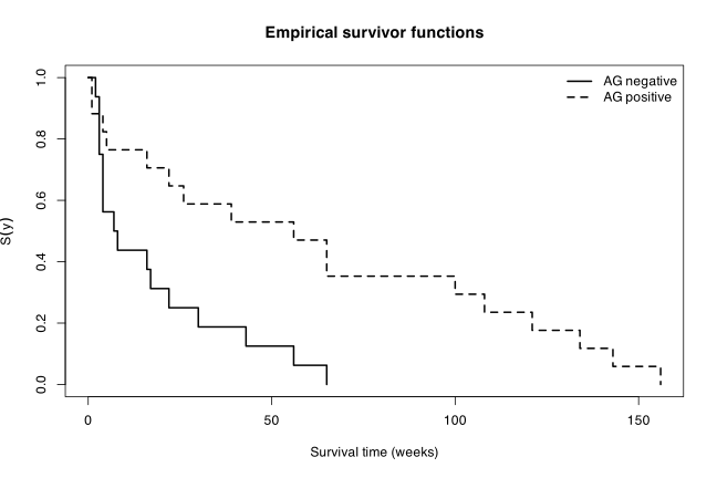
The separation is immediate: the AG negative curve has already fallen to \(0.5\) by week \(7\), whereas the AG positive curve does not cross \(0.5\) until week \(56\). R’s survfit reports medians of \(7.5\) and \(56\) weeks, so median survival is roughly seven times longer in the AG positive group.
Part (b), choosing a distribution. Section 10.6 gives three linearising plots, one per candidate family, and Exercise 10.5(c) supplies the third:
- exponential, from (10.6): \(H(y) = -\log S(y) = \theta y\), so \(-\log \widehat{S}(y)\) against \(y\) should be a straight line through the origin;
- Weibull, from (10.13): \(\log[-\log \widehat{S}(y)]\) against \(\log y\) should be straight with slope \(\lambda\);
- log-logistic, from Exercise 10.5(c): \(\log \widehat{O}(y) = \log[\widehat{S}/(1-\widehat{S})]\) against \(\log y\) should be straight with slope \(-\lambda\).
The final point of each empirical survivor function has \(\widehat{S} = 0\) and is dropped (its log is undefined).
tab <- function(g) {
sub <- subset(leuk, ag == g)
s <- survfit(Surv(time, rep(1, nrow(sub))) ~ 1, data = sub)
d <- data.frame(y = s$time, S = s$surv)
d[d$S > 0 & d$S < 1, ]
}
neg <- tab("-"); pos <- tab("+")
par(mfrow = c(1, 3))
plot(neg$y, -log(neg$S), pch = 16, xlab = "y", ylab = expression(-log~hat(S)(y)),
main = "Exponential check", ylim = range(-log(c(neg$S, pos$S))))
points(pos$y, -log(pos$S), pch = 1)
abline(lm(-log(neg$S) ~ neg$y + 0), lty = 2); abline(lm(-log(pos$S) ~ pos$y + 0), lty = 3)
legend("topleft", c("AG negative", "AG positive"), pch = c(16, 1), bty = "n")
plot(log(neg$y), log(-log(neg$S)), pch = 16, xlab = "log y",
ylab = expression(log~(-log~hat(S)(y))), main = "Weibull check",
xlim = range(log(c(neg$y, pos$y))), ylim = range(log(-log(c(neg$S, pos$S)))))
points(log(pos$y), log(-log(pos$S)), pch = 1)
abline(lm(log(-log(neg$S)) ~ log(neg$y)), lty = 2)
abline(lm(log(-log(pos$S)) ~ log(pos$y)), lty = 3)
plot(log(neg$y), log(neg$S/(1 - neg$S)), pch = 16, xlab = "log y",
ylab = expression(log~hat(O)(y)), main = "Log-logistic check",
xlim = range(log(c(neg$y, pos$y))),
ylim = range(log(c(neg$S, pos$S)/(1 - c(neg$S, pos$S)))))
points(log(pos$y), log(pos$S/(1 - pos$S)), pch = 1)
abline(lm(log(neg$S/(1 - neg$S)) ~ log(neg$y)), lty = 2)
abline(lm(log(pos$S/(1 - pos$S)) ~ log(pos$y)), lty = 3)
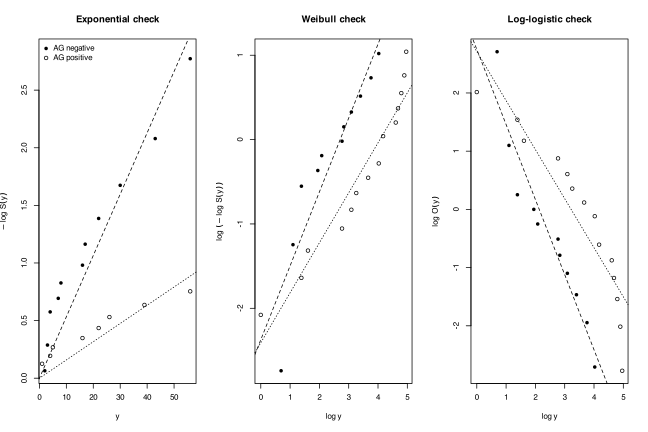
rbind(negative = coef(lm(log(-log(neg$S)) ~ log(neg$y))),
positive = coef(lm(log(-log(pos$S)) ~ log(pos$y))))
(Intercept) log(neg$y)
negative -2.372757 0.8760273
positive -2.408514 0.5925132
The left panel is close to a straight line through the origin in both groups, which already argues for the exponential. In the middle panel the two sets of points are roughly linear, which supports the Weibull family, and the two lines are separated by a roughly constant vertical gap, which supports proportional hazards from (10.9). The fitted slopes are \(0.88\) and \(0.59\); these are crude least squares fits to the Kaplan-Meier points, which give equal weight to the unreliable estimates in the tail, so the apparent difference between them should not be over-read, and the maximum likelihood fit in part (c) puts \(\widehat{\lambda}\) at \(0.96\) for both groups combined. Slopes in this region are consistent with the exponential special case of (10.10), \(\lambda = 1\). The right-hand panel is no straighter than the middle one, so nothing is gained by the log-logistic. Take the exponential as the working model, and check it against the Weibull in part (c).
Part (c), parametric model with the covariate. Fit the proportional hazards models of Section 10.2.2, \(h_j(y) = \exp(\beta_0 + \beta_1 x_{1j} + \beta_2 x_{2j})\) with \(x_1 = 1\) for AG positive and \(x_2 = \log(\mathrm{WBC})\). R’s survreg parameterises the same models as accelerated failure time models, \(\log Y = \mathbf{x}^T\boldsymbol{\alpha} + \sigma W\), so its coefficients are \(-\beta\) for the exponential.
S <- Surv(leuk$time, rep(1, nrow(leuk)))
m.exp <- survreg(S ~ ag + lwbc, data = leuk, dist = "exponential")
m.wei <- survreg(S ~ ag + lwbc, data = leuk, dist = "weibull")
m.llg <- survreg(S ~ ag + lwbc, data = leuk, dist = "loglogistic")
summary(m.exp)
Call:
survreg(formula = S ~ ag + lwbc, data = leuk, dist = "exponential")
Value Std. Error z p
(Intercept) 3.713 0.454 8.17 3e-16
ag+ 1.018 0.364 2.80 0.0051
lwbc -0.304 0.124 -2.45 0.0144
Scale fixed at 1
Exponential distribution
Loglik(model)= -146.5 Loglik(intercept only)= -155.5
Chisq= 17.82 on 2 degrees of freedom, p= 0.00014
Number of Newton-Raphson Iterations: 5
n= 33
c(exponential = AIC(m.exp), weibull = AIC(m.wei), loglogistic = AIC(m.llg),
weibull.scale = m.wei$scale)
exponential weibull loglogistic weibull.scale
299.081049 300.997595 301.164852 1.040689
The Weibull scale is \(\widehat{\sigma} = 1.041\), i.e. shape \(\widehat{\lambda} = 1/\widehat{\sigma} = 0.96\), indistinguishable from the exponential value \(\lambda = 1\); the extra parameter costs two AIC units and buys nothing. The exponential has the smallest AIC of the three and is chosen, exactly as in the remission-time example of Section 10.7.
The same fit can be obtained by the Poisson regression device of Section 10.4: the log-likelihood (10.17) is proportional to that of independent \(D_j \sim \mathrm{Po}(\theta_j y_j)\), with \(\log y_j\) entering as an offset.
g <- glm(rep(1, nrow(leuk)) ~ ag + lwbc + offset(log(time)),
family = stats::poisson(), data = leuk)
round(summary(g)$coefficients, 4)
Estimate Std. Error z value Pr(>|z|)
(Intercept) -3.7127 0.4542 -8.1748 0.0000
ag+ -1.0176 0.3637 -2.7983 0.0051
lwbc 0.3044 0.1244 2.4479 0.0144
The estimates match survreg exactly with the sign reversed, confirming that the Poisson coefficients are the proportional hazards parameters \(\boldsymbol{\beta}\) of (10.8).
Tests of the two terms, and of an interaction, use the deviance-like statistic \(D = 2(\widehat{l}_1 - \widehat{l}_0)\) of Section 10.5:
anova(survreg(S ~ lwbc, data = leuk, dist = "exponential"), m.exp)
anova(m.exp, survreg(S ~ ag * lwbc, data = leuk, dist = "exponential"))
Terms Resid. Df -2*LL Test Df Deviance Pr(>Chi)
1 lwbc 31 300.5704 NA NA NA
2 ag + lwbc 30 293.0810 +ag 1 7.489309 0.006206637
Terms Resid. Df -2*LL Test Df Deviance Pr(>Chi)
1 ag + lwbc 30 293.0810 NA NA NA
2 ag * lwbc 29 291.3166 +ag:lwbc 1 1.764485 0.1840661
Adding AG to a model already containing \(\log(\mathrm{WBC})\) reduces \(-2l\) by \(7.49\) on 1 degree of freedom (\(p = 0.006\)); the AG-by-WBC interaction is not needed (\(D = 1.76\), \(p = 0.18\)), so a single hazard ratio applies at every white cell count.
Interpretation. In the proportional hazards parameterisation the fitted hazard is
\begin{equation*} \widehat{h}(y) = \exp\{-3.713 - 1.018\,x_1 + 0.304\,x_2\}, \end{equation*}
constant in \(y\). The hazard ratio for AG positive versus AG negative, from (10.7), is \(e^{-1.018} = 0.36\) (95% CI \(e^{-1.018 \pm 1.96 \times 0.364} = (0.18, 0.74)\)): at the same white cell count an AG positive patient dies at about one third the rate of an AG negative patient. Equivalently, on the accelerated failure time scale their survival times are stretched by a factor \(e^{1.018} = 2.77\). For WBC the coefficient \(0.304\) means that each unit increase in \(\log(\mathrm{WBC})\) multiplies the hazard by \(e^{0.304} = 1.36\); a doubling of white cell count multiplies it by \(2^{0.304} = 1.23\), so higher counts are bad, as Exercise 4.2(a) already suggested. Mean survival for an AG positive patient with \(\mathrm{WBC} = 10\) is \(1/\widehat{\theta} = \exp(3.713 + 1.018 - 0.304\log 10) = 56\) weeks, against \(20\) weeks for an AG negative patient with the same count.
Part (d), model checking. The Cox-Snell residuals (10.19) are \(r_{Cj} = \widehat{H}_j(y_j) = y_j\widehat{\theta}_j\) for the exponential model; if the model is right they behave like a random sample from the exponential distribution with parameter one, so their mean and variance should both be near \(1\) and an exponential probability plot should follow the line \(y = x\). There is no censoring here, so the \(\Delta\) correction of Section 10.6 is not needed.
rc <- leuk$time / exp(predict(m.exp, type = "lp"))
rd <- residuals(m.exp, type = "deviance")
c(mean = mean(rc), variance = var(rc))
mean variance
1.000000 1.019736
par(mfrow = c(2, 2))
plot(qexp(ppoints(nrow(leuk))), sort(rc), pch = 16,
xlab = "Unit exponential quantiles", ylab = "Ordered Cox-Snell residuals",
main = "Exponential probability plot"); abline(0, 1, lty = 2)
boxplot(rd ~ leuk$ag, xlab = "AG", ylab = "Deviance residuals",
main = "Deviance residuals by group"); abline(h = 0, lty = 2)
plot(leuk$lwbc, rd, pch = 16, xlab = "log(WBC)", ylab = "Deviance residuals",
main = "Deviance residuals vs log(WBC)")
abline(h = 0, lty = 2); lines(lowess(leuk$lwbc, rd), lty = 3)
db <- residuals(m.exp, type = "dfbeta")
plot(seq_len(nrow(leuk)), db[, 2], type = "h", xlab = "Observation",
ylab = expression(Delta[j]*beta[AG]), main = "Delta-betas for the AG effect")
abline(h = 0)
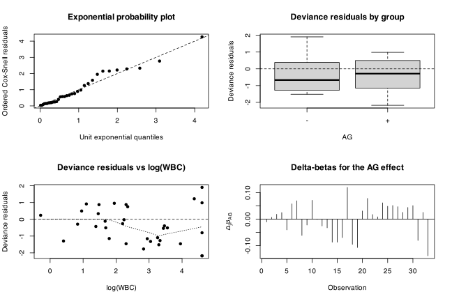
round(rbind(CoxSnell = quantile(rc), deviance = quantile(rd)), 3)
0% 25% 50% 75% 100%
CoxSnell 0.036 0.202 0.633 1.581 4.265
deviance -2.175 -1.266 -0.425 0.496 1.905
The mean of the Cox-Snell residuals is \(1.000\) and their variance \(1.020\), both as the unit exponential requires, and the probability plot is close to the reference line with only mild sagging in the upper tail. Unlike Figure 10.5 for the remission data, the deviance residuals here have very similar distributions in the two groups (means \(-0.39\) and \(-0.34\)), so the AG term has absorbed the group difference rather than leaving it in the residuals. The plot against \(\log(\mathrm{WBC})\) shows a slight downward drift in the lowess line at high counts, but with \(n = 33\) this is weak evidence; the non-significant interaction test in part (c) says the same thing. The most influential single observation for \(\widehat{\beta}_{\mathrm{AG}}\) is subject 33 (an AG negative patient who survived \(43\) weeks despite \(\mathrm{WBC} = 100\)), and dropping it would move the estimate by only \(0.14\), less than half a standard error. The largest deviance residual, \(-2.17\), belongs to subject 14, an AG positive patient with \(\mathrm{WBC} = 100\) who died in week \(1\). Neither point is troubling.
The one genuine reservation is the exponential distribution itself, which by Section 10.2.1 assumes a constant hazard and hence no memory: a leukemia patient who has already survived a year is assumed no more and no less likely to die in the next week than a newly diagnosed one. The empirical checks in part (b) do not contradict this, and the Weibull fit gives \(\widehat{\lambda} = 0.96\), but with 33 observations the data have little power to detect moderate departures.
Part (e), is AG a useful prognostic indicator? Yes. After adjusting for \(\log(\mathrm{WBC})\), AG positivity is associated with a hazard ratio of \(0.36\) (95% CI \(0.18\) to \(0.74\); likelihood ratio \(D = 7.49\) on 1 d.f., \(p = 0.006\)), that is roughly a tripling of expected survival time. The effect is not an artefact of white cell count, since WBC is in the model and the interaction is negligible, and it is not driven by any single patient, as the delta-betas show. The caveats are the small sample, the observational design (AG status is not randomised, so other prognostic factors may be confounded with it) and the strong constant-hazard assumption. Subject to those, AG is worth measuring: it separates patients whose median survival is about two months from patients whose median survival is over a year.
Problem 10.2 — The log-logistic distribution with the probability density function
The log-logistic distribution with the probability density function
\begin{equation*} f(y) = \frac{e^{\theta}\lambda y^{\lambda - 1}}{(1 + e^{\theta}y^{\lambda})^{2}} \end{equation*}
is sometimes used for modelling survival times.
(a) Find the survivor function \(S(y)\), the hazard function \(h(y)\) and the cumulative hazard function \(H(y)\).
(b) Show that the median survival time is \(\exp(-\theta/\lambda)\).
(c) Plot the hazard function for \(\lambda = 1\) and \(\lambda = 5\) with \(\theta = -5\), \(\theta = -2\) and \(\theta = \tfrac{1}{2}\). (difficulty: \(\star\star\))
Throughout \(y \geq 0\), \(\lambda > 0\) and \(\theta\) is unrestricted.
Part (a). Integrate the density directly. Substitute \(u = e^{\theta}t^{\lambda}\), so that \(du = e^{\theta}\lambda t^{\lambda - 1}dt\), which is exactly the numerator of \(f\):
\begin{equation*} F(y) = \int_0^y \frac{e^{\theta}\lambda t^{\lambda-1}}{(1 + e^{\theta}t^{\lambda})^{2}}\,dt = \int_0^{e^{\theta}y^{\lambda}} \frac{du}{(1+u)^{2}} = \left[-\frac{1}{1+u}\right]_0^{e^{\theta}y^{\lambda}} = 1 - \frac{1}{1 + e^{\theta}y^{\lambda}} . \end{equation*}
Hence, from (10.1),
\begin{equation*} S(y) = 1 - F(y) = \frac{1}{1 + e^{\theta}y^{\lambda}} . \end{equation*}
This is a genuine survivor function: \(S(0) = 1\), \(S\) decreases, and \(S(y) \to 0\) as \(y \to \infty\).
The hazard function follows from (10.2):
\begin{equation*} h(y) = \frac{f(y)}{S(y)} = \frac{e^{\theta}\lambda y^{\lambda-1}}{(1 + e^{\theta}y^{\lambda})^{2}}\left(1 + e^{\theta}y^{\lambda}\right) = \frac{e^{\theta}\lambda y^{\lambda-1}}{1 + e^{\theta}y^{\lambda}} , \end{equation*}
which is the baseline hazard \(h_0\) quoted in Exercise 10.4(c). The cumulative hazard is immediate from (10.4):
\begin{equation*} H(y) = -\log S(y) = \log\left(1 + e^{\theta}y^{\lambda}\right) . \end{equation*}
As a check, \(-\dfrac{d}{dy}\log S(y) = \dfrac{d}{dy}\log(1 + e^{\theta}y^{\lambda}) = \dfrac{e^{\theta}\lambda y^{\lambda-1}}{1 + e^{\theta}y^{\lambda}} = h(y)\), agreeing with (10.3).
The name is explained by the survivor function: writing \(Z = \log Y\),
\begin{equation*} \Pr(Z \leq z) = F(e^{z}) = \frac{e^{\theta + \lambda z}}{1 + e^{\theta + \lambda z}} , \end{equation*}
so \(\log Y\) has a logistic distribution with location \(-\theta/\lambda\) and scale \(1/\lambda\). Equivalently \(\mathrm{logit}[F(y)] = \theta + \lambda\log y\), which is the source of the linear log-odds plot of Exercise 10.5(c).
Part (b). The median \(y(50)\) solves \(S(y) = \tfrac{1}{2}\), i.e.
\begin{equation*} \frac{1}{1 + e^{\theta}y^{\lambda}} = \frac{1}{2} \quad\Longleftrightarrow\quad e^{\theta}y^{\lambda} = 1 \quad\Longleftrightarrow\quad y^{\lambda} = e^{-\theta} \quad\Longleftrightarrow\quad y(50) = e^{-\theta/\lambda} . \end{equation*}
It is the median rather than the mean that is quoted because, as Section 10.2 notes, survival distributions are skew; for the log-logistic the mean \(\mathrm{E}(Y) = (\pi/\lambda)e^{-\theta/\lambda}/\sin(\pi/\lambda)\) exists only when \(\lambda > 1\), so for \(\lambda = 1\) there is no finite mean at all and the median is the only usable summary.
Part (c). Before plotting, note the shape analytically. Taking logarithms,
\begin{equation*} \log h(y) = \log\lambda + \theta + (\lambda - 1)\log y - \log\left(1 + e^{\theta}y^{\lambda}\right), \end{equation*}
so
\begin{equation*} \frac{d}{dy}\log h(y) = \frac{\lambda - 1}{y} - \frac{\lambda e^{\theta}y^{\lambda-1}}{1 + e^{\theta}y^{\lambda}} = \frac{(\lambda - 1) - e^{\theta}y^{\lambda}}{y\left(1 + e^{\theta}y^{\lambda}\right)} . \end{equation*}
For \(\lambda \leq 1\) the numerator is negative for all \(y > 0\), so the hazard decreases monotonically from \(h(0^{+}) = e^{\theta}\) when \(\lambda = 1\) (and from \(+\infty\) when \(\lambda < 1\)). For \(\lambda > 1\) the hazard rises from \(0\), peaks at \(y^{\lambda} = (\lambda - 1)e^{-\theta}\), i.e. at \(y = \{(\lambda-1)e^{-\theta}\}^{1/\lambda}\), and then decays like \(\lambda/y\). This eventually-decreasing hazard is what distinguishes the log-logistic from the Weibull (10.12), whose hazard is monotone for every \(\lambda\), and it is why the log-logistic is used for outcomes where risk peaks soon after diagnosis or surgery and then falls away.
h <- function(y, th, lam) lam * exp(th) * y^(lam - 1) / (1 + exp(th) * y^lam)
ths <- c(-5, -2, 0.5)
labs <- c("theta = -5", "theta = -2", "theta = 1/2")
par(mfrow = c(1, 2))
y <- exp(seq(log(0.02), log(1000), length = 600))
for (lam in c(1, 5)) {
plot(NA, xlim = range(y), ylim = c(1e-4, 20), log = "xy", xlab = "y", ylab = "h(y)",
main = bquote(lambda == .(lam)))
for (k in 1:3) lines(y, h(y, ths[k], lam), lty = k, lwd = 2)
for (k in 1:3) abline(v = exp(-ths[k]/lam), col = "grey60", lty = 3)
legend(if (lam == 1) "bottomleft" else "topright", labs, lty = 1:3, lwd = 2, bty = "n")
}
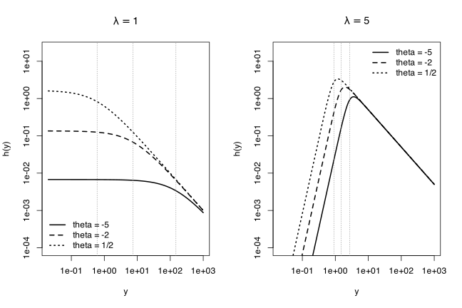
Both axes are logarithmic, because the six curves live on very different scales; the vertical grey lines mark the medians \(e^{-\theta/\lambda}\) from part (b).
mode5 <- function(th) ((5 - 1) * exp(-th))^(1/5)
rbind(theta = ths, median.lam1 = exp(-ths), h0.lam1 = exp(ths),
median.lam5 = exp(-ths/5), mode.lam5 = mode5(ths),
peak.h.lam5 = mapply(function(t) h(mode5(t), t, 5), ths))
[,1] [,2] [,3]
theta -5.000000000 -2.0000000 0.5000000
median.lam1 148.413159103 7.3890561 0.6065307
h0.lam1 0.006737947 0.1353353 1.6487213
median.lam5 2.718281828 1.4918247 0.9048374
mode.lam5 3.586794376 1.9684745 1.1939401
peak.h.lam5 1.115201927 2.0320304 3.3502517
Reading the plot. In the left panel (\(\lambda = 1\)) the log-logistic reduces to a hazard \(e^{\theta}/(1 + e^{\theta}y)\) that starts at \(e^{\theta}\) and decreases monotonically, approaching \(1/y\) regardless of \(\theta\); the three curves are therefore ordered by \(\theta\) at small \(y\) and merge at large \(y\). Lowering \(\theta\) shifts survival to later times: the median moves from \(0.61\) at \(\theta = \tfrac{1}{2}\) to \(148\) at \(\theta = -5\). In the right panel (\(\lambda = 5\)) every curve is unimodal, rising steeply as \(y^{4}\), peaking at \(y = \{4e^{-\theta}\}^{1/5}\) (that is, at \(3.59\), \(1.97\) and \(1.19\) for the three values of \(\theta\)) and then falling as \(5/y\). The parameter \(\theta\) acts purely as a scale shift on the time axis, since \(h(y;\theta,\lambda)\) depends on \(\theta\) and \(y\) only through \(e^{\theta}y^{\lambda}\) apart from the factor \(y^{\lambda-1}\); the parameter \(\lambda\) controls the shape, deciding whether the hazard is monotone decreasing or hump-shaped.
Problem 10.3 — For accelerated failure time models the explanatory variables for subject
For accelerated failure time models the explanatory variables for subject \(i\), \(\eta_i\), act multiplicatively on the time variable so that the hazard function for subject \(i\) is
\begin{equation*} h_i(y) = \eta_i h_0(\eta_i y), \end{equation*}
where \(h_0(y)\) is the baseline hazard function. Show that the Weibull and log-logistic distributions both have this property but the exponential distribution does not. (Hint: Obtain the hazard function for the random variable \(T = \eta_i Y\).) (difficulty: \(\star\star\))
First the general mechanism behind the definition. Let \(Y\) have baseline survivor function \(S_0\) and hazard \(h_0\), and let subject \(i\) have survival time \(T_i = Y/\eta_i\), so that a large \(\eta_i\) compresses the time scale and a small \(\eta_i\) stretches it. Then
\begin{equation*} S_i(y) = \Pr(T_i \geq y) = \Pr(Y \geq \eta_i y) = S_0(\eta_i y), \end{equation*}
and by (10.3),
\begin{equation*} h_i(y) = -\frac{d}{dy}\log S_i(y) = -\frac{d}{dy}\log S_0(\eta_i y) = \eta_i h_0(\eta_i y), \end{equation*}
by the chain rule. So the displayed equation is not an extra assumption: it is what a multiplicative change of the time scale always does to a hazard function. (Equivalently, in the hint’s direction, if \(T = \eta_i Y\) then \(h_T(t) = \eta_i^{-1}h_0(\eta_i^{-1}t)\), the same statement with \(\eta_i\) replaced by \(\eta_i^{-1}\).)
What has to be shown, therefore, is a closure property: that \(\eta h_0(\eta y)\) is again a member of the same parametric family, so that the accelerated model can be written down with the same distribution and a covariate-dependent parameter. Note also that \(\log T_i = \log Y - \log\eta_i\), so an accelerated failure time model is a location model for \(\log Y\) with the covariates entering the location; this is exactly the survreg parameterisation used in Exercise 10.1.
Weibull. From (10.12) the baseline hazard is \(h_0(y) = \lambda\phi y^{\lambda-1}\). Then
\begin{equation*} \eta h_0(\eta y) = \eta\,\lambda\phi(\eta y)^{\lambda-1} = \lambda\left(\eta^{\lambda}\phi\right)y^{\lambda-1}, \end{equation*}
which is again a Weibull hazard, with the same shape parameter \(\lambda\) and with \(\phi\) replaced by
\begin{equation*} \phi_i = \eta_i^{\lambda}\phi . \end{equation*}
So the Weibull family is closed under acceleration, and the accelerated failure time model is obtained simply by letting \(\phi\) depend on the covariates. Taking \(\eta_i = e^{\mathbf{x}_i^T\boldsymbol{\gamma}}\) gives \(\phi_i = \phi e^{\mathbf{x}_i^T(\lambda\boldsymbol{\gamma})}\), which is precisely the multiplicative form \(\phi = \alpha e^{\mathbf{x}^T\boldsymbol{\beta}}\) used at the top of page 230 with \(\boldsymbol{\beta} = \lambda\boldsymbol{\gamma}\). This is why the Weibull is the one distribution that is simultaneously an accelerated failure time model and a proportional hazards model (Exercise 10.4(b)): the two parameterisations differ only by the factor \(\lambda\).
Log-logistic. From Exercise 10.2(a) the baseline hazard is \(h_0(y) = e^{\theta}\lambda y^{\lambda-1}/(1 + e^{\theta}y^{\lambda})\). Then
\begin{equation*} \eta h_0(\eta y) = \frac{\eta\, e^{\theta}\lambda(\eta y)^{\lambda-1}}{1 + e^{\theta}(\eta y)^{\lambda}} = \frac{\left(e^{\theta}\eta^{\lambda}\right)\lambda y^{\lambda-1}}{1 + \left(e^{\theta}\eta^{\lambda}\right)y^{\lambda}} , \end{equation*}
since the factor \(\eta \cdot \eta^{\lambda-1} = \eta^{\lambda}\) can be absorbed into the constant. This is again a log-logistic hazard with the same \(\lambda\) and with
\begin{equation*} \theta_i = \theta + \lambda\log\eta_i . \end{equation*}
So the log-logistic family is also closed, and putting \(\eta_i = e^{\mathbf{x}_i^T\boldsymbol{\gamma}}\) gives the linear model \(\theta_i = \theta + \mathbf{x}_i^T(\lambda\boldsymbol{\gamma})\) for the location parameter. The same conclusion is visible from Exercise 10.2(a) without any calculus: \(\log Y\) is logistic with location \(-\theta/\lambda\) and scale \(1/\lambda\), and subtracting \(\log\eta_i\) from a logistic variable shifts its location while leaving its scale alone.
Exponential. The baseline hazard is the constant \(h_0(y) = \theta\), so
\begin{equation*} \eta h_0(\eta y) = \eta\theta , \end{equation*}
which is again a constant. The algebra is degenerate: because \(h_0\) does not depend on \(y\) at all, the acceleration \(y \mapsto \eta y\) inside the argument has no effect whatsoever, and all that survives is the leading factor \(\eta\). Two consequences follow.
- The exponential model has no accelerated failure time structure distinct from a rescaling of the hazard. The identity \(h_i(y) = \eta_i h_0(\eta_i y) = \eta_i h_0(y)\) is simultaneously the proportional hazards model (10.20), so the parameter \(\eta_i\) is not identifiable as an acceleration factor: compressing the time scale and multiplying the hazard rate are the same operation. In the Weibull and log-logistic cases the two operations are genuinely different, and (as the Weibull calculation shows) they are related by the factor \(\lambda\); for the exponential \(\lambda = 1\) and the distinction collapses.
- Equivalently, the exponential hazard cannot change shape. The defining feature of an accelerated failure time model is that the subject’s hazard is the baseline hazard viewed on a stretched or compressed clock, so the peak of the hazard, its rate of increase, and so on all move with \(\eta_i\). A constant hazard has no such features to move.
One point of rigour is worth stating plainly. Read as a bare closure statement the exponential does satisfy the equation, since \(\eta\theta\) is again an exponential hazard. The sense in which the exponential lacks the property, and the sense in which the remark on page 230 calls the Weibull the only distribution with both properties, is the degeneracy just described: acceleration must act on the shape of the hazard and not merely on its level, and for the exponential there is no shape to act on. That is the version proved above.
A simulation confirms the two closure results, using the inverse-survivor transformations \(Y = \{e^{-\theta}(1/U - 1)\}^{1/\lambda}\) for the log-logistic and \(Y = \{-\log(U)/\phi\}^{1/\lambda}\) for the Weibull, with \(U\) uniform:
set.seed(2026)
qs <- c(.1, .25, .5, .75, .9)
n <- 2e5; eta <- 2.5
rllog <- function(n, th, lam) { u <- runif(n); (exp(-th) * (1/u - 1))^(1/lam) }
qllog <- function(p, th, lam) (exp(-th) * (1/(1 - p) - 1))^(1/lam)
th <- -2; lam <- 3
Tt <- rllog(n, th, lam) / eta
round(rbind(simulated = quantile(Tt, qs),
theoretical = qllog(qs, th + lam * log(eta), lam)), 4)
10% 25% 50% 75% 90%
simulated 0.3740 0.5390 0.7771 1.1237 1.6166
theoretical 0.3745 0.5402 0.7791 1.1236 1.6206
lam <- 1.7; phi <- 0.4
Tt <- (-log(runif(n))/phi)^(1/lam) / eta
qwei <- function(p, lam, phi) (-log(1 - p)/phi)^(1/lam)
round(rbind(simulated = quantile(Tt, qs),
theoretical = qwei(qs, lam, eta^lam * phi)), 4)
10% 25% 50% 75% 90%
simulated 0.1828 0.3306 0.5538 0.8322 1.1192
theoretical 0.1825 0.3295 0.5527 0.8310 1.1200
Dividing a log-logistic time by \(\eta\) reproduces a log-logistic distribution with \(\theta\) shifted by \(\lambda\log\eta\), and dividing a Weibull time by \(\eta\) reproduces a Weibull distribution with \(\phi\) multiplied by \(\eta^{\lambda}\), as derived.
Problem 10.4 — For proportional hazards models the explanatory variables for subject
For proportional hazards models the explanatory variables for subject \(i\), \(\eta_i\), act multiplicatively on the hazard function. If \(\eta_i = e^{\mathbf{x}_i^T\boldsymbol{\beta}}\), then the hazard function for subject \(i\) is
\begin{equation*} h_i(y) = e^{\mathbf{x}_i^T\boldsymbol{\beta}}h_0(y), \tag{10.20} \end{equation*}
where \(h_0(y)\) is the baseline hazard function.
(a) For the exponential distribution if \(h_0 = \theta\), show that if \(\theta_i = e^{\mathbf{x}_i^T\boldsymbol{\beta}}\theta\) for the \(i\)th subject, then (10.20) is satisfied.
(b) For the Weibull distribution if \(h_0 = \lambda\phi y^{\lambda-1}\), show that if \(\phi_i = e^{\mathbf{x}_i^T\boldsymbol{\beta}}\phi\) for the \(i\)th subject, then (10.20) is satisfied.
(c) For the log-logistic distribution if \(h_0 = e^{\theta}\lambda y^{\lambda-1}/(1 + e^{\theta}y^{\lambda})\), show that if \(e^{\theta_i} = e^{\theta + \mathbf{x}_i^T\boldsymbol{\beta}}\) for the \(i\)th subject, then (10.20) is not satisfied. Hence, or otherwise, deduce that the log-logistic distribution does not have the proportional hazards property. (difficulty: \(\star\star\))
Write \(\eta_i = e^{\mathbf{x}_i^T\boldsymbol{\beta}}\) throughout. In each part the subject-specific hazard is obtained by substituting the subject’s parameter into the hazard formula and comparing with \(h_0\).
Part (a), exponential. The hazard of the exponential distribution (10.5) is the constant \(\theta\) (Section 10.2.1). With \(\theta_i = \eta_i\theta\) the \(i\)th subject’s hazard is
\begin{equation*} h_i(y) = \theta_i = \eta_i\theta = e^{\mathbf{x}_i^T\boldsymbol{\beta}}h_0(y), \end{equation*}
so (10.20) holds identically in \(y\), with \(h_0(y) = \theta\) the hazard at the reference levels (\(\mathbf{x}_i = \mathbf{0}\)). This is the model of Section 10.2.2, \(h(y;\boldsymbol{\beta}) = e^{\mathbf{x}^T\boldsymbol{\beta}}\) after absorbing \(\theta\) into an intercept \(\beta_0 = \log\theta\), and it is the model fitted to the leukemia data in Exercise 10.1(c). The hazard ratio (10.7) for a binary \(x_k\) is \(e^{\beta_k}\), constant in \(y\).
Part (b), Weibull. From (10.12) the hazard is \(h(y;\lambda,\phi) = \lambda\phi y^{\lambda-1}\). The shape parameter \(\lambda\) is held fixed and only \(\phi\) carries the covariates, \(\phi_i = \eta_i\phi\), so
\begin{equation*} h_i(y) = \lambda\phi_i y^{\lambda-1} = \lambda\,\eta_i\phi\,y^{\lambda-1} = e^{\mathbf{x}_i^T\boldsymbol{\beta}}\lambda\phi y^{\lambda-1} = e^{\mathbf{x}_i^T\boldsymbol{\beta}}h_0(y), \end{equation*}
and (10.20) is satisfied for every \(y\). This is exactly (10.14) with \(\phi = \alpha e^{\mathbf{x}^T\boldsymbol{\beta}}\). It is essential that \(\lambda\) does not vary between subjects: if it did, the ratio \(h_i(y)/h_0(y)\) would carry a factor \(y^{\lambda_i - \lambda}\) and would not be constant. Combining this with Exercise 10.3, the Weibull is both an accelerated failure time family and a proportional hazards family, the two parameterisations being linked by \(\boldsymbol{\beta} = \lambda\boldsymbol{\gamma}\).
Part (c), log-logistic. Substituting \(e^{\theta_i} = \eta_i e^{\theta}\) into the hazard of Exercise 10.2(a),
\begin{equation*} h_i(y) = \frac{e^{\theta_i}\lambda y^{\lambda-1}}{1 + e^{\theta_i}y^{\lambda}} = \frac{\eta_i e^{\theta}\lambda y^{\lambda-1}}{1 + \eta_i e^{\theta}y^{\lambda}} , \end{equation*}
so the hazard ratio is
\begin{equation*} \frac{h_i(y)}{h_0(y)} = \eta_i\,\frac{1 + e^{\theta}y^{\lambda}}{1 + \eta_i e^{\theta}y^{\lambda}} . \end{equation*}
The covariate factor \(\eta_i\) appears in the denominator as well as the numerator, and the ratio is a genuine function of \(y\) unless \(\eta_i = 1\). Its behaviour at the two ends of the time scale is
\begin{equation*} \lim_{y \to 0}\frac{h_i(y)}{h_0(y)} = \eta_i , \qquad \lim_{y \to \infty}\frac{h_i(y)}{h_0(y)} = \eta_i \cdot \frac{e^{\theta}y^{\lambda}}{\eta_i e^{\theta}y^{\lambda}} = 1 . \end{equation*}
The ratio therefore starts at \(\eta_i\) and decays monotonically to \(1\): the hazards of the two groups converge, and (10.20) fails. Equivalently, the cumulative hazards \(H_i(y) = \log(1 + \eta_i e^{\theta}y^{\lambda})\) do not differ by a constant, so the log-cumulative-hazard curves of Section 10.6 are not parallel, which is the diagnostic consequence.
A numerical illustration with \(\theta = -2\), \(\lambda = 3\) and \(\eta_i = 3\), alongside the Weibull for contrast:
h <- function(y, th, lam) lam * exp(th) * y^(lam - 1) / (1 + exp(th) * y^lam)
th <- -2; lam <- 3; xb <- log(3); y <- c(0.01, 0.1, 0.5, 1, 2, 5, 20)
round(rbind(y = y,
ratio.loglogistic = h(y, th + xb, lam) / h(y, th, lam),
ratio.weibull = (lam * exp(xb) * 0.4 * y^(lam - 1)) /
(lam * 0.4 * y^(lam - 1))), 4)
[,1] [,2] [,3] [,4] [,5] [,6] [,7]
y 0.01 0.1000 0.5000 1.0000 2.0000 5.0000 20.0000
ratio.loglogistic 3.00 2.9992 2.9034 2.4225 1.4708 1.0386 1.0006
ratio.weibull 3.00 3.0000 3.0000 3.0000 3.0000 3.0000 3.0000
The Weibull ratio is exactly \(e^{\mathbf{x}^T\boldsymbol{\beta}} = 3\) at every time, while the log-logistic ratio falls from \(3\) to \(1\) over the range of the data.
Deducing that no log-logistic model has proportional hazards. Part (c) shows that one particular parameterisation fails, which by itself leaves open the possibility that some other way of letting the parameters depend on covariates would succeed. It does not. Suppose two log-logistic distributions, with parameters \((\theta_1,\lambda_1)\) and \((\theta_0,\lambda_0)\), had proportional hazards, so that for some constant \(c > 0\)
\begin{equation*} \frac{h(y;\theta_1,\lambda_1)}{h(y;\theta_0,\lambda_0)} = \frac{\lambda_1}{\lambda_0}\,e^{\theta_1 - \theta_0}\,y^{\lambda_1 - \lambda_0}\, \frac{1 + e^{\theta_0}y^{\lambda_0}}{1 + e^{\theta_1}y^{\lambda_1}} = c \quad\text{for all } y > 0 . \end{equation*}
Let \(y \to 0\). The last fraction tends to \(1\), so the left side behaves like \((\lambda_1/\lambda_0)e^{\theta_1-\theta_0}y^{\lambda_1-\lambda_0}\), which has a finite non-zero limit only if \(\lambda_1 = \lambda_0 = \lambda\). With the shapes equal the condition becomes
\begin{equation*} e^{\theta_1 - \theta_0}\,\frac{1 + e^{\theta_0}y^{\lambda}}{1 + e^{\theta_1}y^{\lambda}} = c , \end{equation*}
whose value is \(e^{\theta_1-\theta_0}\) at \(y \to 0\) and \(1\) at \(y \to \infty\). A constant that equals both forces \(e^{\theta_1-\theta_0} = 1\), that is \(\theta_1 = \theta_0\), and then \(c = 1\) and the two distributions coincide. Hence no non-trivial proportional hazards model can be built inside the log-logistic family.
The point is structural rather than parameterisational. By Exercise 10.2(a) the log-logistic hazard is eventually decreasing like \(\lambda/y\) whatever the parameters, so any two members of the family have hazards that merge at large \(y\); proportionality with a ratio different from \(1\) is impossible. What the log-logistic does possess instead is the proportional odds property, which is the subject of Exercise 10.5.
Problem 10.5 — As the survivor function S(y) is the probability of surviving beyond time
As the survivor function \(S(y)\) is the probability of surviving beyond time \(y\), the odds of survival past time \(y\) are
\begin{equation*} O(y) = \frac{S(y)}{1 - S(y)} . \end{equation*}
For proportional odds models the explanatory variables for subject \(i\), \(\eta_i\), act multiplicatively on the odds of survival beyond time \(y\),
\begin{equation*} O_i = \eta_i O_0 , \end{equation*}
where \(O_0\) is the baseline odds.
(a) Find the odds of survival beyond time \(y\) for the exponential, Weibull and log-logistic distributions.
(b) Show that only the log-logistic distribution has the proportional odds property.
(c) For the log-logistic distribution show that the log odds of survival beyond time \(y\) are
\begin{equation*} \log O(y) = \log\left[\frac{S(y)}{1 - S(y)}\right] = -\theta - \lambda\log y . \end{equation*}
Therefore, if \(\log \widehat{O}_i\) (estimated from the empirical survivor function) plotted against \(\log y\) is approximately linear, then the log-logistic distribution may provide a suitable model.
(d) From (b) and (c) deduce that for two groups of subjects with explanatory variables \(\eta_1\) and \(\eta_2\) plots of \(\log \widehat{O}_1\) and \(\log \widehat{O}_2\) against \(\log y\) should produce approximately parallel straight lines. (difficulty: \(\star\star\))
Part (a), odds of survival. In each case substitute the survivor function into \(O = S/(1-S)\).
Exponential, from (10.6) \(S(y) = e^{-\theta y}\):
\begin{equation*} O(y) = \frac{e^{-\theta y}}{1 - e^{-\theta y}} = \frac{1}{e^{\theta y} - 1} . \end{equation*}
Weibull, from (10.11) \(S(y) = \exp(-\phi y^{\lambda})\):
\begin{equation*} O(y) = \frac{\exp(-\phi y^{\lambda})}{1 - \exp(-\phi y^{\lambda})} = \frac{1}{\exp(\phi y^{\lambda}) - 1} . \end{equation*}
The exponential is the case \(\lambda = 1\), \(\phi = \theta\), as it must be.
Log-logistic, from Exercise 10.2(a) \(S(y) = 1/(1 + e^{\theta}y^{\lambda})\), so \(1 - S(y) = e^{\theta}y^{\lambda}/(1 + e^{\theta}y^{\lambda})\) and
\begin{equation*} O(y) = \frac{1/(1 + e^{\theta}y^{\lambda})}{e^{\theta}y^{\lambda}/(1 + e^{\theta}y^{\lambda})} = \frac{1}{e^{\theta}y^{\lambda}} = e^{-\theta}y^{-\lambda} . \end{equation*}
The log-logistic odds are a pure power function of \(y\); the other two are not.
Part (b), only the log-logistic has proportional odds. Proportional odds requires the ratio \(O_i(y)/O_0(y)\) to be a constant \(\eta_i\) for all \(y > 0\).
Log-logistic. Here \(O(y) = e^{-\theta}y^{-\lambda}\), so for two members of the family with the same shape \(\lambda\),
\begin{equation*} \frac{O_i(y)}{O_0(y)} = \frac{e^{-\theta_i}y^{-\lambda}}{e^{-\theta}y^{-\lambda}} = e^{\theta - \theta_i} , \end{equation*}
free of \(y\). Setting \(\theta_i = \theta - \log\eta_i\), or \(\theta_i = \theta - \mathbf{x}_i^T\boldsymbol{\beta}\) in a regression, gives \(O_i(y) = \eta_i O_0(y)\) exactly. So the log-logistic family is a proportional odds family, with the covariates entering the location parameter \(\theta\) linearly. (Contrast Exercise 10.4(c): the very same reparameterisation destroys proportional hazards. A distribution can have one property or the other; the log-logistic has odds, the Weibull has hazards.)
Weibull, and the exponential as its special case. Suppose \(O_i(y)/O_0(y) = c\) for all \(y\), where subject \(i\) has parameters \((\lambda_i,\phi_i)\) and the baseline has \((\lambda,\phi)\). Examine the two tails.
As \(y \to 0\), \(\exp(\phi y^{\lambda}) - 1 = \phi y^{\lambda}\{1 + O(y^{\lambda})\}\), so \(O(y) \sim 1/(\phi y^{\lambda})\) and
\begin{equation*} \frac{O_i(y)}{O_0(y)} \sim \frac{\phi}{\phi_i}\,y^{\lambda - \lambda_i} . \end{equation*}
For this to have a finite non-zero limit we need \(\lambda_i = \lambda\), and then the limit is \(\phi/\phi_i\).
As \(y \to \infty\), \(O(y) \sim \exp(-\phi y^{\lambda})\), so with \(\lambda_i = \lambda\),
\begin{equation*} \frac{O_i(y)}{O_0(y)} \sim \exp\left\{(\phi - \phi_i)y^{\lambda}\right\} , \end{equation*}
which tends to \(0\) if \(\phi_i > \phi\) and to \(\infty\) if \(\phi_i < \phi\). A constant ratio therefore forces \(\phi_i = \phi\), that is \(c = 1\) and the two distributions are identical. Hence no non-trivial proportional odds model exists inside the Weibull family, and setting \(\lambda = 1\) throughout gives the same conclusion for the exponential. The underlying reason is that the Weibull and exponential survivor functions decay exponentially fast, so their log-odds fall away like \(-\phi y^{\lambda}\), whereas proportional odds requires the log-odds curves to be vertical translates of one another and hence to have the same shape.
The three cases are easy to see on the \(\log O\) against \(\log y\) scale of part (c), each panel comparing a baseline with a curve whose parameter has been multiplied by \(3\):
y <- exp(seq(log(0.02), log(50), length = 500))
lo <- function(S) log(S/(1 - S))
par(mfrow = c(1, 3))
th <- 0.3
plot(log(y), lo(exp(-th*y)), type = "l", lwd = 2, ylim = c(-8, 6),
xlab = "log y", ylab = expression(log~O(y)), main = "Exponential")
lines(log(y), lo(exp(-3*th*y)), lwd = 2, lty = 2)
legend("bottomleft", c("baseline", "eta = 3 on hazard"), lty = 1:2, lwd = 2, bty = "n")
lam <- 2; phi <- 0.3
plot(log(y), lo(exp(-phi*y^lam)), type = "l", lwd = 2, ylim = c(-8, 6),
xlab = "log y", ylab = expression(log~O(y)), main = "Weibull")
lines(log(y), lo(exp(-3*phi*y^lam)), lwd = 2, lty = 2)
Sll <- function(y, th, lam) 1/(1 + exp(th)*y^lam)
th <- -2; lam <- 2
plot(log(y), lo(Sll(y, th, lam)), type = "l", lwd = 2, ylim = c(-8, 6),
xlab = "log y", ylab = expression(log~O(y)), main = "Log-logistic")
lines(log(y), lo(Sll(y, th + log(3), lam)), lwd = 2, lty = 2)
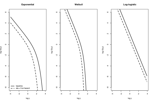
Only the third panel shows two straight lines separated by a constant vertical distance. In the first two panels the curves bend and the gap between them widens without limit as \(y\) increases.
Part (c), log odds for the log-logistic. Taking logarithms of the odds found in part (a),
\begin{equation*} \log O(y) = \log\left(e^{-\theta}y^{-\lambda}\right) = -\theta - \lambda\log y , \end{equation*}
a straight line in \(\log y\) with intercept \(-\theta\) and slope \(-\lambda\). Equivalently, and more transparently, \(\mathrm{logit}[1 - S(y)] = \theta + \lambda\log y\): the log-logistic is precisely the distribution whose cumulative distribution function is logistic in \(\log y\), which is the sense in which it is the survival-time analogue of the logistic regression model of Chapter 7.
This gives the diagnostic plot. Compute the empirical survivor function \(\widehat{S}(y)\) of Section 10.3, form \(\log\widehat{O}(y) = \log[\widehat{S}(y)/\{1 - \widehat{S}(y)\}]\) and plot it against \(\log y\). Approximate linearity supports the log-logistic; the intercept estimates \(-\theta\) and minus the slope estimates \(\lambda\). This is the third panel of the diagnostic figure in Exercise 10.1(b) and it is the log-logistic counterpart of the two plots given in Section 10.6, namely \(-\log\widehat{S}(y)\) against \(y\) for the exponential and \(\log[-\log\widehat{S}(y)]\) against \(\log y\) for the Weibull, from (10.13). The points with \(\widehat{S} = 0\) or \(\widehat{S} = 1\) must be dropped, since their log-odds are infinite.
Part (d), two groups. Suppose the two groups follow log-logistic distributions with a common shape \(\lambda\) and multipliers \(\eta_1\) and \(\eta_2\) on the odds, so by (b) their parameters are \(\theta_g = \theta - \log\eta_g\) for \(g = 1, 2\). Taking logarithms of \(O_g = \eta_g O_0\) and using (c),
\begin{equation*} \log O_g(y) = \log\eta_g + \log O_0(y) = \left(\log\eta_g - \theta\right) - \lambda\log y , \qquad g = 1, 2 . \end{equation*}
Both are straight lines in \(\log y\) with the same slope \(-\lambda\), and their vertical separation is
\begin{equation*} \log O_1(y) - \log O_2(y) = \log\left(\frac{\eta_1}{\eta_2}\right) = \theta_2 - \theta_1 , \end{equation*}
constant in \(y\). So the two plots of \(\log \widehat{O}_g\) against \(\log y\) should be approximately parallel straight lines, and the vertical gap between them estimates the log odds ratio \(\log(\eta_1/\eta_2)\), in exact analogy with the parallel log-cumulative-hazard lines that diagnose proportional hazards in (10.9) and Section 10.6.
Read the other way, the plot is a two-part diagnostic. Curvature of either line says the log-logistic distribution is wrong; straight but non-parallel lines say the log-logistic may be right for each group separately but the proportional odds assumption fails, so the groups differ in shape \(\lambda\) as well as in location. Both this plot and the log-cumulative-hazard plot are applied to the hepatitis data in Exercise 10.6(b).
Problem 10.6 — The data in Table 10.5 are survival times, in months, of 44 patients with
The data in Table 10.5 are survival times, in months, of 44 patients with chronic active hepatitis. They participated in a randomized controlled trial of prednisolone compared with no treatment. There were 22 patients in each group. One patient was lost to follow-up and several in each group were still alive at the end of the trial. The data are from Altman and Bland (1998).
Table 10.5 gives the survival times in months, where an asterisk marks a censored time and a double asterisk marks the patient lost to follow-up. Prednisolone group: 2, 6, 12, 54, 56**, 68, 89, 96, 96, 125*, 128*, 131*, 140*, 141*, 143, 145*, 146, 148*, 162*, 168, 173*, 181*. No treatment group: 2, 3, 4, 7, 10, 22, 28, 29, 32, 37, 40, 41, 54, 61, 63, 71, 127*, 140*, 146*, 158*, 167*, 182*.
(a) Calculate the empirical survivor functions for each group.
(b) Use suitable plots to investigate the properties of accelerated failure times, proportional hazards and proportional odds, using the results from Exercises 10.3, 10.4 and 10.5, respectively.
(c) Based on the results from (b) fit an appropriate model to the data in Table 10.5 to estimate the relative effect of prednisolone. (difficulty: \(\star\star\star\))
The data are the hepatitis data frame in the dobson package. The patient lost to follow-up at 56 months contributes exactly the same information as a censored observation, namely that his survival time exceeded 56 months, so he is coded as censored; this assumes that loss to follow-up is unrelated to prognosis, which cannot be checked from these data.
Part (a), empirical survivor functions. With censoring present the Kaplan-Meier product limit estimate of Section 10.3 is required, and only death times contribute a step.
library(dobson)
library(survival)
data(hepatitis, package = "dobson")
hep <- data.frame(time = hepatitis[["survival time"]],
dead = as.integer(hepatitis$censor == "died"),
grp = factor(hepatitis$group,
levels = c("no treatment", "prednisolone")))
table(hep$grp, hep$dead)
km <- survfit(Surv(time, dead) ~ grp, data = hep)
km
0 1
no treatment 6 16
prednisolone 11 11
Call: survfit(formula = Surv(time, dead) ~ grp, data = hep)
n events median 0.95LCL 0.95UCL
grp=no treatment 22 16 40.5 29 NA
grp=prednisolone 22 11 146.0 96 NA
summary(km)
Call: survfit(formula = Surv(time, dead) ~ grp, data = hep)
grp=no treatment
time n.risk n.event survival std.err lower 95% CI upper 95% CI
2 22 1 0.955 0.0444 0.871 1.000
3 21 1 0.909 0.0613 0.797 1.000
4 20 1 0.864 0.0732 0.732 1.000
7 19 1 0.818 0.0822 0.672 0.996
10 18 1 0.773 0.0893 0.616 0.969
22 17 1 0.727 0.0950 0.563 0.939
28 16 1 0.682 0.0993 0.513 0.907
29 15 1 0.636 0.1026 0.464 0.873
32 14 1 0.591 0.1048 0.417 0.837
37 13 1 0.545 0.1062 0.372 0.799
40 12 1 0.500 0.1066 0.329 0.759
41 11 1 0.455 0.1062 0.288 0.718
54 10 1 0.409 0.1048 0.248 0.676
61 9 1 0.364 0.1026 0.209 0.632
63 8 1 0.318 0.0993 0.173 0.587
71 7 1 0.273 0.0950 0.138 0.540
grp=prednisolone
time n.risk n.event survival std.err lower 95% CI upper 95% CI
2 22 1 0.955 0.0444 0.871 1.000
6 21 1 0.909 0.0613 0.797 1.000
12 20 1 0.864 0.0732 0.732 1.000
54 19 1 0.818 0.0822 0.672 0.996
68 17 1 0.770 0.0904 0.612 0.969
89 16 1 0.722 0.0967 0.555 0.939
96 15 2 0.626 0.1051 0.450 0.870
143 8 1 0.547 0.1175 0.359 0.834
146 6 1 0.456 0.1285 0.263 0.793
168 3 1 0.304 0.1509 0.115 0.804
plot(km, lty = c(1, 2), lwd = 2, xlab = "Survival time (months)",
ylab = expression(hat(S)(y)), mark.time = TRUE,
main = "Chronic active hepatitis: Kaplan-Meier estimates")
legend("bottomleft", c("no treatment", "prednisolone"), lty = c(1, 2), lwd = 2, bty = "n")
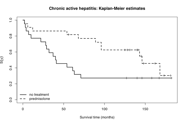
Median survival is \(40.5\) months without treatment against \(146\) months with prednisolone. The censoring pattern is very different in the two arms: 16 of the 22 untreated patients died against 11 of the 22 treated, and in the treated arm the censored times are concentrated after 125 months, so the right-hand end of the treated curve rests on very few patients (three at risk at 168 months) and its confidence band is wide.
Part (b), which of the three structures fits? Each of the three properties has a linearising plot, all built from the same Kaplan-Meier estimates and all requiring the observations with \(\widehat{S} = 0\) or \(\widehat{S} = 1\) to be dropped.
- Accelerated failure times (Exercise 10.3). Under a Weibull accelerated failure time model, (10.13) gives \(\log[-\log \widehat{S}(y)] = \log\phi + \lambda\log y\), so the plot of \(\log[-\log\widehat{S}(y)]\) against \(\log y\) should be straight in each group. Under a log-logistic accelerated failure time model the log-odds plot below should be straight instead. Straightness diagnoses the distribution; the acceleration itself is a horizontal shift of the curve.
- Proportional hazards (Exercise 10.4). From (10.9) the two log cumulative hazard curves should be parallel, separated by \(\beta_k\). So the same plot serves twice: straight lines diagnose the Weibull, parallel lines diagnose proportional hazards, and the slope estimates \(\lambda\).
- Proportional odds (Exercise 10.5(c) and (d)). The plot of \(\log\widehat{O}(y) = \log[\widehat{S}/(1-\widehat{S})]\) against \(\log y\) should give two parallel straight lines of slope \(-\lambda\).
get <- function(g) {
s <- survfit(Surv(time, dead) ~ 1, data = subset(hep, grp == g))
d <- data.frame(y = s$time, S = s$surv, n = s$n.event)
d[d$n > 0 & d$S > 0 & d$S < 1, ]
}
nt <- get("no treatment"); pr <- get("prednisolone")
par(mfrow = c(1, 2))
plot(log(nt$y), log(-log(nt$S)), pch = 16, xlab = "log y",
ylab = expression(log~(-log~hat(S)(y))), main = "Log cumulative hazard",
xlim = range(log(c(nt$y, pr$y))), ylim = range(log(-log(c(nt$S, pr$S)))))
points(log(pr$y), log(-log(pr$S)), pch = 1)
abline(lm(log(-log(nt$S)) ~ log(nt$y)), lty = 2)
abline(lm(log(-log(pr$S)) ~ log(pr$y)), lty = 3)
legend("topleft", c("no treatment", "prednisolone"), pch = c(16, 1), bty = "n")
plot(log(nt$y), log(nt$S/(1 - nt$S)), pch = 16, xlab = "log y",
ylab = expression(log~hat(O)(y)), main = "Log odds of survival",
xlim = range(log(c(nt$y, pr$y))),
ylim = range(log(c(nt$S, pr$S)/(1 - c(nt$S, pr$S)))))
points(log(pr$y), log(pr$S/(1 - pr$S)), pch = 1)
abline(lm(log(nt$S/(1 - nt$S)) ~ log(nt$y)), lty = 2)
abline(lm(log(pr$S/(1 - pr$S)) ~ log(pr$y)), lty = 3)
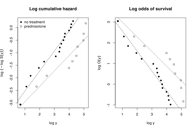
round(rbind(
cumhaz.no.treatment = coef(lm(log(-log(nt$S)) ~ log(nt$y))),
cumhaz.prednisolone = coef(lm(log(-log(pr$S)) ~ log(pr$y))),
logodds.no.treatment = coef(lm(log(nt$S/(1 - nt$S)) ~ log(nt$y))),
logodds.prednisolone = coef(lm(log(pr$S/(1 - pr$S)) ~ log(pr$y)))), 3)
(Intercept) log(nt$y)
cumhaz.no.treatment -3.333 0.803
cumhaz.prednisolone -3.572 0.616
logodds.no.treatment 3.522 -0.963
logodds.prednisolone 3.705 -0.710
Both plots are acceptably straight, so both the Weibull and the log-logistic are plausible distributions; neither shows the pronounced curvature that would rule a family out. Both are also acceptably parallel, so both proportional hazards and proportional odds are tenable. The fitted slopes are \(0.80\) and \(0.62\) for the log cumulative hazard and \(-0.96\) and \(-0.71\) for the log odds; in each case the treated group has the flatter line, but with only 16 and 11 death times, and with the treated points confined to the right-hand part of the range, the difference in slopes is within what sampling variation would produce.
Two substantive readings follow. First, the log-cumulative-hazard slopes are around \(0.7\), appreciably below \(1\), which points to a Weibull with \(\lambda < 1\), that is a hazard that falls with time: the risk of death is highest soon after entry and declines among survivors, which is clinically plausible for chronic active hepatitis. The exponential, with its constant hazard, is therefore suspect here in a way it was not for the leukemia data of Exercise 10.1. Second, the fact that both plots work about equally well is not surprising, since with \(n = 44\) and heavy censoring the data cannot distinguish sharply between families whose survivor functions differ only in the tails; the choice will have to be made on likelihood grounds in part (c).
Part (c), fitting and interpreting a model. All four candidate parametric models are fitted by maximum likelihood using the censored likelihood (10.15), and compared by AIC as in Section 10.7.
S <- Surv(hep$time, hep$dead)
fits <- list(exponential = survreg(S ~ grp, data = hep, dist = "exponential"),
weibull = survreg(S ~ grp, data = hep, dist = "weibull"),
loglogistic = survreg(S ~ grp, data = hep, dist = "loglogistic"),
lognormal = survreg(S ~ grp, data = hep, dist = "lognormal"))
round(sapply(fits, function(f) c(coef(f), scale = f$scale,
logLik = as.numeric(logLik(f)), AIC = AIC(f))), 4)
exponential weibull loglogistic lognormal
(Intercept) 4.4886 4.4811 3.8182 3.8522
grpprednisolone 0.9009 1.0544 1.3272 1.2496
scale 1.0000 1.2673 0.9831 1.7752
logLik -158.1025 -157.0170 -156.3152 -156.7166
AIC 320.2051 320.0339 318.6303 319.4332
The log-logistic has the smallest AIC, but the whole spread is only \(1.6\) units, so the evidence between families is weak; the diagnostic plots said the same thing. The Weibull scale is \(1.267\), giving \(\widehat{\lambda} = 1/1.267 = 0.79\), matching the empirical slopes in part (b) and confirming a decreasing hazard, though the test of \(\lambda = 1\) is not significant (\(\log\widehat{\sigma} = 0.237\), s.e. \(0.169\)). The log-logistic scale is \(0.983\), giving \(\widehat{\lambda} = 1.02\).
I take the log-logistic as the primary model, since it has the best AIC and since the proportional odds structure of Exercise 10.5 is the one it supports, and report the Weibull proportional hazards fit alongside it.
summary(fits$loglogistic)
Call:
survreg(formula = S ~ grp, data = hep, dist = "loglogistic")
Value Std. Error z p
(Intercept) 3.8182 0.3671 10.40 <2e-16
grpprednisolone 1.3272 0.5349 2.48 0.013
Log(scale) -0.0171 0.1678 -0.10 0.919
Scale= 0.983
Log logistic distribution
Loglik(model)= -156.3 Loglik(intercept only)= -159.2
Chisq= 5.85 on 1 degrees of freedom, p= 0.016
Number of Newton-Raphson Iterations: 4
n= 44
survreg writes the model as \(\log Y = \mu_g + \sigma W\) with \(W\) standard logistic, so in the notation of Exercise 10.2 the parameters are \(\lambda = 1/\sigma\) and \(\theta_g = -\mu_g/\sigma\). Three summaries of the treatment effect follow.
m <- fits$loglogistic; b <- coef(m); sg <- m$scale
se <- sqrt(vcov(m)[2, 2]); ci <- b[2] + c(-1, 1) * 1.96 * se
round(c(lambda = 1/sg, median.no.treatment = exp(b[1]),
median.prednisolone = exp(b[1] + b[2]),
time.ratio = exp(b[2]), tr.lo = exp(ci[1]), tr.hi = exp(ci[2]),
odds.ratio = exp(b[2]/sg), or.lo = exp(ci[1]/sg), or.hi = exp(ci[2]/sg)), 3)
lambda median.no.treatment.(Intercept)
1.017 45.523
median.prednisolone.(Intercept) time.ratio.grpprednisolone
171.636 3.770
tr.lo tr.hi
1.321 10.758
odds.ratio.grpprednisolone or.lo
3.857 1.328
or.hi
11.207
Interpretation. The fitted median survival, \(e^{-\theta/\lambda} = e^{\mu}\) from Exercise 10.2(b), is \(45.5\) months without treatment and \(171.6\) months with prednisolone; these bracket the Kaplan-Meier medians of \(40.5\) and \(146\) months from part (a). On the accelerated failure time scale of Exercise 10.3 prednisolone multiplies survival time by \(\widehat{\eta} = e^{1.327} = 3.77\) (95% CI \(1.32\) to \(10.76\)), that is it stretches the whole survival distribution by a factor of nearly four. On the proportional odds scale of Exercise 10.5 the odds of surviving beyond any given time are multiplied by \(\exp(1.327/0.983) = 3.86\) (95% CI \(1.33\) to \(11.21\)). The Wald test gives \(z = 2.48\), \(p = 0.013\), and the likelihood ratio statistic of Section 10.5 is \(D = 2(\widehat{l}_1 - \widehat{l}_0) = 5.85\) on 1 degree of freedom, \(p = 0.016\).
The Weibull fit tells the same story in the hazard metric of (10.20). Since \(\phi_g = \exp(-\mu_g/\sigma)\), the hazard ratio is \(\exp(-\widehat{\beta}_{\mathrm{AFT}}/\widehat{\sigma})\):
mw <- fits$weibull; me <- fits$exponential
round(c(weibull.lambda = 1/mw$scale,
weibull.HR = exp(-coef(mw)[2]/mw$scale),
exponential.HR = exp(-coef(me)[2]),
exp.HR.lo = exp(-(coef(me)[2] + 1.96*sqrt(vcov(me)[2,2]))),
exp.HR.hi = exp(-(coef(me)[2] - 1.96*sqrt(vcov(me)[2,2])))), 3)
weibull.lambda weibull.HR.grpprednisolone
0.789 0.435
exponential.HR.grpprednisolone exp.HR.lo.grpprednisolone
0.406 0.189
exp.HR.hi.grpprednisolone
0.875
Prednisolone roughly halves the death rate, \(\widehat{HR} = 0.44\) under the Weibull and \(0.41\) under the exponential. Two model-free checks agree: the log-rank test of the two Kaplan-Meier curves and the Cox proportional hazards model (semi-parametric, and so outside the scope of this chapter, but a useful benchmark).
survdiff(S ~ grp, data = hep)
summary(coxph(S ~ grp, data = hep))$conf.int
Call:
survdiff(formula = S ~ grp, data = hep)
N Observed Expected (O-E)^2/E (O-E)^2/V
grp=no treatment 22 16 10.6 2.73 4.66
grp=prednisolone 22 11 16.4 1.77 4.66
Chisq= 4.7 on 1 degrees of freedom, p= 0.03
exp(coef) exp(-coef) lower .95 upper .95
grpprednisolone 0.4357837 2.294716 0.2000254 0.9494164
The Cox estimate \(\widehat{HR} = 0.436\) (95% CI \(0.20\) to \(0.95\)) is indistinguishable from the Weibull estimate \(0.435\), which is reassuring: the parametric assumption is buying precision without distorting the point estimate.
Model checking. The fitted log-logistic survivor curves are overlaid on the Kaplan-Meier estimates, and the Cox-Snell residuals (10.19) \(r_{Cj} = \widehat{H}_j(y_j) = \log(1 + e^{\widehat{\theta}_g}y_j^{\widehat{\lambda}})\) are checked by estimating their own survivor function (retaining the original censoring indicators) and plotting \(-\log\widehat{S}(r_C)\) against \(r_C\); a well-fitting model gives points on the line through the origin with slope one, since the residuals should then be a censored sample from the unit exponential.
par(mfrow = c(1, 2))
plot(km, lty = c(1, 2), lwd = 2, xlab = "Survival time (months)",
ylab = expression(hat(S)(y)), mark.time = TRUE,
main = "Kaplan-Meier and fitted log-logistic")
lam <- 1/m$scale; th <- -b[1]/m$scale; th2 <- -(b[1] + b[2])/m$scale
yy <- seq(1, 200, length = 400)
lines(yy, 1/(1 + exp(th)*yy^lam), col = "grey40", lwd = 2)
lines(yy, 1/(1 + exp(th2)*yy^lam), col = "grey40", lwd = 2, lty = 2)
legend("bottomleft", c("no treatment", "prednisolone"), lty = c(1, 2), lwd = 2, bty = "n")
rc <- log(1 + exp(ifelse(hep$grp == "no treatment", th, th2)) * hep$time^lam)
sr <- survfit(Surv(rc, hep$dead) ~ 1)
plot(sr$time, -log(sr$surv), pch = 16, xlab = "Cox-Snell residual",
ylab = expression(-log~hat(S)(r[C])), main = "Cox-Snell residual plot")
abline(0, 1, lty = 2)
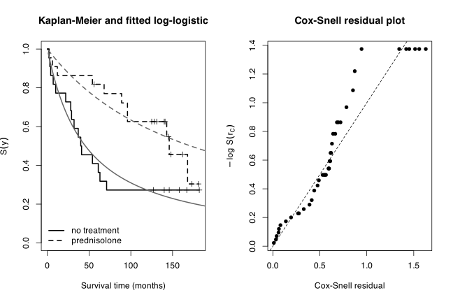
The fitted curves track the two Kaplan-Meier estimates reasonably. The clearest discrepancy is early in the treated arm, where the observed curve is flat between 12 and 54 months while the smooth log-logistic curve is already falling; a distribution with a hazard that starts near zero, such as a Weibull with \(\lambda > 1\), would fit that stretch better but would fit the untreated arm worse. In the Cox-Snell plot the points sit a little above the reference line through the middle of the range and then flatten out at the top, where the last few residuals belong to censored observations and \(\widehat{S}(r_C)\) is estimated from a handful of patients. Neither feature is large, and the flattening at the right is the usual artefact of a Kaplan-Meier estimate whose largest observations are censored rather than evidence of misfit.
Conclusion. Prednisolone materially improves survival in chronic active hepatitis. The estimated effect is a hazard ratio of about \(0.44\), equivalently an odds-of-survival ratio of about \(3.9\), equivalently a stretching of survival times by a factor of about \(3.8\), with median survival rising from roughly \(46\) to roughly \(172\) months. The effect is statistically significant at the 5% level by every test applied (\(p\) between \(0.01\) and \(0.04\)) but the confidence intervals are wide, the lower limit for the time ratio being only \(1.3\); 44 patients and 27 deaths do not pin the effect down closely. The choice between the three structures cannot be made from these data: accelerated failure times, proportional hazards and proportional odds all describe them about equally well, and the conclusion about prednisolone is the same under each, which is the practically important point.
Clustered and Longitudinal Data
Problem 11.1 — The measurement of left ventricular volume of the heart is important for
The measurement of left ventricular volume of the heart is important for studies of cardiac physiology and clinical management of patients with heart disease. An indirect way of measuring the volume, \(y\), involves a measurement called parallel conductance volume, \(x\). Boltwood et al. (1989) found an approximately linear association between \(y\) and \(x\) in a study of dogs under various “load” conditions. The results, reported by Glantz and Slinker (1990), are shown in Table 11.9: measurements of left ventricular volume \(y\) and parallel conductance volume \(x\) on five dogs under eight different load conditions.
Dog 1: \(y\) = 81.7, 84.3, 72.8, 71.7, 76.7, 75.8, 77.3, 86.3; \(x\) = 54.3, 62.0, 62.3, 47.3, 53.6, 38.0, 54.2, 54.0. Dog 2: \(y\) = 105.0, 113.6, 108.7, 83.9, 89.0, 86.1, 88.7, 117.6; \(x\) = 81.5, 80.8, 74.5, 71.9, 79.5, 73.0, 74.7, 88.6. Dog 3: \(y\) = 95.5, 95.7, 84.0, 85.8, 98.8, 106.2, 106.4, 115.0; \(x\) = 65.0, 68.3, 67.9, 61.0, 66.0, 81.8, 71.4, 96.0. Dog 4: \(y\) = 113.1, 116.5, 100.8, 101.5, 120.8, 95.0, 91.9, 94.0; \(x\) = 87.5, 93.6, 70.4, 66.1, 101.4, 57.0, 82.5, 80.9. Dog 5: \(y\) = 99.5, 99.2, 106.1, 85.2, 106.3, 84.6, 92.1, 101.2; \(x\) = 79.4, 82.5, 87.9, 66.4, 68.4, 59.5, 58.5, 69.2.
- (a)
- Conduct an exploratory analysis of these data.
- (b)
- Let \((Y_{jk}, x_{jk})\) denote the \(k\)th measurement on dog \(j\), (\(j = 1, \ldots, 5\); \(k = 1, \ldots, 8\)). Fit the linear model
\begin{equation*} \mathrm{E}(Y_{jk}) = \mu = \alpha + \beta x_{jk}, \qquad Y \sim \mathrm{N}(\mu, \sigma^2), \end{equation*}
assuming the random variables \(Y_{jk}\) are independent (i.e., ignoring the repeated measures on the same dogs). Compare the estimates of the intercept \(\alpha\) and slope \(\beta\) and their standard errors from this pooled analysis with the results you obtain using a data reduction approach.
- (c)
- Fit a suitable random effects model.
- (d)
- Fit a clustered model using a GEE.
- (e)
- Compare the results you obtain from each approach. Which method(s) do you think are most appropriate? Why?
(difficulty: \(\star\star\star\))
The design is clustered rather than longitudinal: the “conditions” \(k = 1, \ldots, 8\) are experimentally imposed load states, not times, so there is no natural ordering along \(k\) and an exchangeable correlation structure (11.7) is the natural first choice. Each dog is a cluster of size \(K = 8\) and there are only \(J = 5\) clusters. That last number governs everything that follows: five is a very small number of independent units, so every method here is being asked to work near the edge of its asymptotics.
(a) Exploratory analysis.
library(dobson)
data(dogs)
dogs <- as.data.frame(dogs)
dogs$dog <- factor(dogs$dog)
aggregate(cbind(y, x) ~ dog, data = dogs,
FUN = function(v) c(mean = mean(v), sd = sd(v)))
round(cor(dogs$y, dogs$x), 3)
sapply(split(dogs, dogs$dog), function(d) round(cor(d$y, d$x), 3))
dog y.mean y.sd x.mean x.sd
1 1 78.325000 5.280354 53.212500 7.829511
2 2 99.075000 13.573477 78.062500 5.606358
3 3 98.425000 10.572032 72.175000 11.393325
4 4 104.200000 11.115498 79.925000 14.738458
5 5 96.775000 8.574339 71.475000 10.732294
[1] 0.806
1 2 3 4 5
0.305 0.752 0.825 0.725 0.663
Dog 1 sits well below the others on both variables (mean \(y = 78.3\) against \(97\)–\(104\), mean \(x = 53.2\) against \(71\)–\(80\)), which is the clustering made visible: a dog with a small heart gives eight small \(y\)’s and eight small \(x\)’s. The pooled correlation, \(0.806\), is therefore inflated by between-dog contrast; the within-dog correlations are all smaller and range from \(0.31\) (dog 1) to \(0.83\) (dog 3).
par(mfrow = c(1, 2), mar = c(4.5, 4.5, 2.5, 1))
cols <- c("black", "red", "blue", "darkgreen", "purple")
plot(dogs$x, dogs$y, col = cols[dogs$dog], pch = 16,
xlab = "parallel conductance volume x", ylab = "LV volume y",
main = "Pooled scatter with per-dog lines")
for (j in levels(dogs$dog)) {
d <- dogs[dogs$dog == j, ]
abline(lm(y ~ x, data = d), col = cols[as.integer(j)], lty = 2)
}
abline(lm(y ~ x, data = dogs), lwd = 2)
legend("bottomright", legend = paste("dog", 1:5), col = cols, pch = 16, bty = "n")
matplot(1:8, matrix(dogs$y, nrow = 8), type = "b", pch = 16, lty = 1, col = cols,
xlab = "load condition", ylab = "LV volume y",
main = "Profiles by load condition")
dev.off()
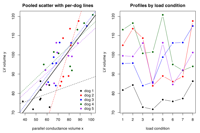
The left panel shows the five per-dog lines fanning out rather than lying parallel. Dogs 3, 4 and 5 give lines of similar slope to the heavy pooled line; dog 1 is much flatter; and dog 2’s line is close to vertical, because its eight \(x\) values span only \(71.9\) to \(88.6\) while its \(y\) values span \(83.9\) to \(117.6\). The right panel shows that the profiles share a common shape across conditions — a pronounced dip at condition 4, a second dip at 6, a rise at 8 — but no monotone trend in \(k\), which is what one expects when \(k\) indexes load states rather than times. Dog 1’s profile lies clear below the other four, which is the visual signature of a dog effect.
The between/within split can be made explicit by decomposing \(x\) into its dog mean \(\bar{x}_{j\cdot}\) and the deviation \(x_{jk} - \bar{x}_{j\cdot}\):
xbar <- tapply(dogs$x, dogs$dog, mean); ybar <- tapply(dogs$y, dogs$dog, mean)
round(coef(lm(ybar ~ xbar)), 3)
dogs$xb <- xbar[dogs$dog]; dogs$xw <- dogs$x - dogs$xb
round(summary(lm(y ~ xw + xb, data = dogs))$coef, 4)
(Intercept) xbar
29.958 0.922
Estimate Std. Error t value Pr(>|t|)
(Intercept) 29.9584 9.2653 3.2334 0.0026
xw 0.6288 0.1242 5.0617 0.0000
xb 0.9215 0.1294 7.1212 0.0000
The between-dog slope is \(0.92\) and the within-dog slope is \(0.63\). They are different questions: \(0.63\) is how much \(y\) moves when you change the load on a given dog, \(0.92\) is how much bigger \(y\) is for a dog whose conductance volume is bigger. Boltwood’s calibration question is the within-dog one.
(b) Pooled analysis versus data reduction.
pooled <- lm(y ~ x, data = dogs)
summary(pooled)
Coefficients:
Estimate Std. Error t value Pr(>|t|)
(Intercept) 40.76808 6.61726 6.161 3.43e-07 ***
x 0.76923 0.09156 8.401 3.42e-10 ***
Residual standard error: 7.911 on 38 degrees of freedom
Multiple R-squared: 0.65, Adjusted R-squared: 0.6408
F-statistic: 70.58 on 1 and 38 DF, p-value: 3.416e-10
So \(\hat{\alpha} = 40.77\) (s.e. \(6.62\)), \(\hat{\beta} = 0.769\) (s.e. \(0.0916\)), on 38 residual degrees of freedom. The 38 is the problem: there are 40 observations but only 5 independent dogs, so the nominal degrees of freedom are a fiction unless the within-dog correlation really is zero.
Before comparing, the fit itself should be checked.
par(mfrow = c(1, 3), mar = c(4.5, 4.5, 2.5, 1))
plot(fitted(pooled), rstandard(pooled), pch = 16, col = dogs$dog,
xlab = "fitted", ylab = "standardised residual", main = "Residuals vs fitted")
abline(h = 0, lty = 2)
boxplot(rstandard(pooled) ~ dogs$dog, xlab = "dog", ylab = "standardised residual",
main = "Residuals by dog")
abline(h = 0, lty = 2)
qqnorm(rstandard(pooled), pch = 16, main = "Normal Q-Q")
qqline(rstandard(pooled))
dev.off()
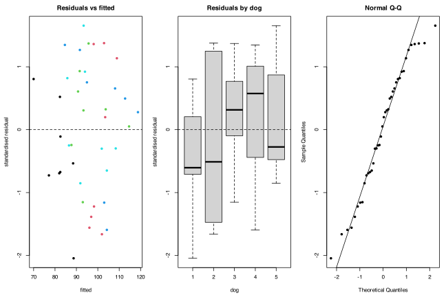
The residuals show no curvature and no change of spread across the fitted range, and the Q-Q plot is close to a straight line, so the Normal linear model is adequate as far as the marginal assumptions go. The middle panel is the one that matters for this chapter: if there were a strong dog effect the five boxes would be displaced from zero and each box would be narrow. Instead all five straddle zero and all five are wide, which foreshadows the zero variance component found in part (c). The residual spread is largest for dog 2, the animal whose fitted line is the outlier.
The data reduction approach of Section 11.2 fits a separate line to each dog and then treats the five intercepts and five slopes as the data:
co <- t(sapply(split(dogs, dogs$dog), function(d) coef(lm(y ~ x, data = d))))
round(co, 3)
round(rbind(mean = colMeans(co), se = apply(co, 2, sd) / sqrt(5)), 3)
t.test(co[, 2])
(Intercept) x
1 67.389 0.206
2 -43.076 1.821
3 43.178 0.765
4 60.514 0.547
5 58.892 0.530
(Intercept) x
mean 37.38 0.774
se 20.50 0.277
One Sample t-test
data: co[, 2]
t = 2.7967, df = 4, p-value = 0.04897
alternative hypothesis: true mean is not equal to 0
95 percent confidence interval:
0.005610799 1.541811613
sample estimates:
mean of x
0.7737112
The two point estimates of \(\beta\) agree almost exactly (\(0.769\) versus \(0.774\)) and the intercepts agree tolerably (\(40.8\) versus \(37.4\)), but the standard errors do not: \(0.277\) against \(0.0916\), a factor of \(3.0\), and \(20.5\) against \(6.6\) for the intercept. This is the same phenomenon as in Tables 11.3 and 11.5–11.6 for the stroke data. The pooled analysis counts 40 independent observations; the data reduction analysis counts 5, and on 4 degrees of freedom the slope only just reaches significance (\(p = 0.049\)).
The inflation here is driven almost entirely by dog 2, whose fitted slope is \(1.82\) against \(0.21\)–\(0.77\) for the others. Dog 2 has the narrowest \(x\) range in the study, so its slope is the least well determined, but the data reduction approach weights all five subject-specific estimates equally and ignores their very different precisions — exactly the drawback Dobson notes at the end of Section 11.2, where the subject-specific analysis is said to ignore “the random error in the estimates.” The standard error of \(0.277\) is therefore honest about the number of independent units but inefficient, because it treats five estimates of very unequal quality as five equally informative observations.
(c) Random effects model. The natural two-level model puts a random intercept on dog:
\begin{equation*} Y_{jk} = \alpha + \beta x_{jk} + b_j + e_{jk}, \qquad b_j \sim \mathrm{N}(0, \sigma_b^2), \quad e_{jk} \sim \mathrm{N}(0, \sigma^2), \end{equation*}
independently. This induces exactly the equicorrelation matrix (11.7) with \(\rho = \sigma_b^2 / (\sigma_b^2 + \sigma^2)\), i.e. compound symmetry.
library(lme4)
m1 <- lmer(y ~ x + (1 | dog), data = dogs, REML = TRUE)
summary(m1)
boundary (singular) fit: see help('isSingular')
Linear mixed model fit by REML ['lmerMod']
Formula: y ~ x + (1 | dog)
Random effects:
Groups Name Variance Std.Dev.
dog (Intercept) 0.00 0.000
Residual 62.58 7.911
Number of obs: 40, groups: dog, 5
Fixed effects:
Estimate Std. Error t value
(Intercept) 40.76808 6.61726 6.161
x 0.76923 0.09156 8.401
The between-dog variance is estimated at the boundary, \(\hat{\sigma}_b^2 = 0\), so the mixed model collapses onto the pooled fit of part (b) — identical estimates and identical standard errors. This is not a software failure; it is a finding. Once \(x\) is in the model there is nothing left for a dog effect to explain, because the dog means of \(y\) and of \(x\) move together (the between-dog slope of \(0.92\) found in part (a)). Fitting dog as a fixed factor instead makes the same point:
round(summary(lm(y ~ x + dog, data = dogs))$coef, 4)
a <- anova(lm(resid(lm(y ~ x, data = dogs)) ~ dogs$dog))
MSB <- a[1, 3]; MSW <- a[2, 3]
round(c(MSB = MSB, MSW = MSW, rho = (MSB - MSW) / (MSB + 7 * MSW)), 3)
Estimate Std. Error t value Pr(>|t|)
(Intercept) 44.8626 7.2807 6.1619 0.0000
x 0.6288 0.1264 4.9746 0.0000
dog2 5.1232 5.0386 1.0168 0.3164
dog3 8.1755 4.6114 1.7729 0.0852
dog4 9.0770 5.1886 1.7494 0.0892
dog5 6.9657 4.5660 1.5256 0.1364
MSB MSW rho
47.716 62.490 -0.030
None of the four dog contrasts is significant at the 5% level. The second calculation is the usual one-way moment estimator of the intra-class correlation applied to the residuals from the pooled fit,
\begin{equation*} \widehat{\rho} = \frac{\mathrm{MS}_{\text{between}} - \mathrm{MS}_{\text{within}}}{\mathrm{MS}_{\text{between}} + (K-1)\mathrm{MS}_{\text{within}}} , \end{equation*}
with \(K = 8\). The between-dog mean square, \(47.7\), is smaller than the within-dog mean square, \(62.5\), so \(\widehat{\rho} = -0.030\). A variance component cannot be negative, so the likelihood is maximised on the boundary and \(\widehat{\sigma}_b^2\) is pinned at zero.
Allowing the slope to vary as well does not help:
m2 <- lmer(y ~ x + (x | dog), data = dogs, REML = TRUE)
anova(update(m1, REML = FALSE), update(m2, REML = FALSE))
Data: dogs
Models:
update(m1, REML = FALSE): y ~ x + (1 | dog)
update(m2, REML = FALSE): y ~ x + (x | dog)
npar AIC BIC logLik -2*log(L) Chisq Df Pr(>Chisq)
update(m1, REML = FALSE) 4 284.92 291.68 -138.46 276.92
update(m2, REML = FALSE) 6 288.94 299.08 -138.47 276.94 0 2 1
The random slope model is also singular (estimated intercept-slope correlation exactly \(-1\)), the deviance does not drop at all, and AIC rises by 4. There is not enough information in five dogs to estimate a slope variance. The random intercept model is the one to report, with the honest conclusion \(\hat{\sigma}_b^2 = 0\), \(\hat{\beta} = 0.769\) (s.e. \(0.092\)).
(d) GEE. Now model the correlation directly rather than through a random effect, solving (11.12) with the identity link and Gaussian variance function, and using the sandwich estimator of Section 11.3 for the standard errors.
library(geepack)
gi <- geeglm(y ~ x, id = dog, data = dogs, family = gaussian, corstr = "independence")
ge <- geeglm(y ~ x, id = dog, data = dogs, family = gaussian, corstr = "exchangeable")
ga <- geeglm(y ~ x, id = dog, waves = condition, data = dogs,
family = gaussian, corstr = "ar1")
for (g in list(gi, ge, ga)) {
cat("corstr =", g$corstr, "\n")
print(round(summary(g)$coefficients, 4))
if (nrow(summary(g)$corr) > 0) print(round(summary(g)$corr, 4))
cat("\n")
}
corstr = independence
Estimate Std.err Wald Pr(>|W|)
(Intercept) 40.7681 4.5237 81.2165 0
x 0.7692 0.0518 220.6030 0
corstr = exchangeable
Estimate Std.err Wald Pr(>|W|)
(Intercept) 36.5514 3.9915 83.8541 0
x 0.8286 0.0481 296.5865 0
Estimate Std.err
alpha -0.0769 0.0342
corstr = ar1
Estimate Std.err Wald Pr(>|W|)
(Intercept) 46.3112 5.2577 77.5852 0
x 0.6941 0.0626 122.8725 0
Estimate Std.err
alpha 0.2858 0.1021
The three working correlation structures give \(\hat{\beta} = 0.769\), \(0.829\) and \(0.694\) — a spread of about \(0.13\), comfortably inside one data-reduction standard error, which illustrates Liang and Zeger’s robustness result quoted in Section 11.4: the point estimate is not very sensitive to \(R_i\). The exchangeable fit estimates \(\hat{\alpha}_{\text{corr}} = -0.077\), which is small and negative like the moment estimate \(-0.030\) of part (c) and again says there is no positive clustering left after adjusting for \(x\). The AR(1) fit should be discounted: the load conditions have no time ordering, so \(\rho^{|j-k|}\) has no meaning here, and its apparent \(\hat{\alpha} = 0.286\) is an artefact of the conditions happening to be listed in an order that groups similar loads together.
The sandwich standard errors are the striking feature: \(0.052\) for the slope under independence, against \(0.092\) from the same point estimate fitted by least squares. The robust standard error is smaller, not larger. With \(J = 5\) clusters the sandwich matrix \(C = \sum_j \mathbf{x}_j^T \hat{\mathbf{V}}_j^{-1} (\mathbf{y}_j - \mathbf{x}_j \hat{\beta}) (\mathbf{y}_j - \mathbf{x}_j \hat{\beta})^T \hat{\mathbf{V}}_j^{-1} \mathbf{x}_j\) is a sum of only five rank-one terms and is badly downward biased; the estimator is consistent as \(J \to \infty\) and 5 is not close to \(\infty\). These GEE standard errors should not be believed.
(e) Comparison.
| Method | \(\hat{\alpha}\) | s.e. | \(\hat{\beta}\) | s.e. |
|---|---|---|---|---|
| Pooled OLS (ignores clusters) | 40.77 | 6.62 | 0.769 | 0.0916 |
| Data reduction (5 dog lines) | 37.38 | 20.50 | 0.774 | 0.2770 |
| Random intercept (lmer) | 40.77 | 6.62 | 0.769 | 0.0916 |
| GEE, independence, sandwich | 40.77 | 4.52 | 0.769 | 0.0518 |
| GEE, exchangeable, sandwich | 36.55 | 3.99 | 0.829 | 0.0481 |
| Dog as fixed factor (within) | 44.86 | 7.28 | 0.629 | 0.1264 |
Every method puts \(\hat{\beta}\) between \(0.63\) and \(0.83\), so the substantive conclusion is stable: left ventricular volume rises by roughly \(0.7\)–\(0.8\) units per unit of parallel conductance volume, and the association is unambiguously present. The methods disagree only about precision, by a factor of five in the standard error, and the disagreement is entirely about how many independent units the study contains.
Which to prefer. The random effects model of part (c) is the most appropriate as a description, because it is the only one that asks whether there is a dog effect rather than assuming one; here it answers no, and its estimated correlation structure then reduces to independence. That answer is what licenses the pooled analysis of part (b), which would otherwise be indefensible. The data reduction estimate is the most defensible interval, since it uses only the five genuinely independent units and requires no assumption about the within-dog covariance, but it is inefficient because it discards the very unequal precisions of the five subject-specific slopes (dog 2 contributes as much as dog 3 despite a much narrower \(x\) range). The GEE analysis of part (d) is the least trustworthy of the four: Section 11.7 recommends Wald statistics with the robust sandwich estimator for GEE inference, but that recommendation rests on the consistency result of Liang and Zeger (1986) quoted in Section 11.4, which is asymptotic in the number of clusters. With \(J = 5\) that justification is absent, and the sandwich standard errors here are visibly anticonservative.
One further caution about interpretation. All the marginal fits above estimate a blend of the within-dog slope \(0.63\) and the between-dog slope \(0.92\). If the scientific question is calibration — how does \(y\) respond when the load on a given animal is changed? — then \(0.63\) from the fixed-dog fit, or equivalently the coefficient of the centred \(x\) in part (a), is the estimate to quote, and the pooled \(0.769\) is biased upward by the between-dog contrast. Five animals is too few to say whether the difference between \(0.63\) and \(0.92\) is real, so this remains a caution rather than a conclusion.
Problem 11.2 — Suppose that (Y jk , x jk ) are observations on the kth subject in cluster k (with
Suppose that \((Y_{jk}, x_{jk})\) are observations on the \(k\)th subject in cluster \(j\) (with \(j = 1, \ldots, J\); \(k = 1, \ldots, K\)) and the goal is to fit a “regression through the origin” model
\begin{equation*} \mathrm{E}(Y_{jk}) = \beta x_{jk}, \end{equation*}
where the variance-covariance matrix for \(Y\)’s in the same cluster is the \(K \times K\) equicorrelation matrix
\begin{equation*} \mathbf{V}_j = \sigma^2 \begin{bmatrix} 1 & \rho & \cdots & \rho \\ \rho & 1 & & \rho \\ \vdots & & \ddots & \vdots \\ \rho & \rho & \cdots & 1 \end{bmatrix}, \end{equation*}
that is, every diagonal element is \(\sigma^2\) and every off-diagonal element is \(\sigma^2 \rho\), and \(Y\)’s in different clusters are independent.
- (a)
- From Section 11.3, if the \(Y\)’s are Normally distributed, then
\begin{equation*} \widehat{\boldsymbol{\beta}} = \Bigl( \sum_{j=1}^{J} \mathbf{x}_j^T \mathbf{V}_j^{-1} \mathbf{x}_j \Bigr)^{-1} \Bigl( \sum_{j=1}^{J} \mathbf{x}_j^T \mathbf{V}_j^{-1} \mathbf{y}_j \Bigr) \quad \text{with} \quad \mathrm{var}(\widehat{\boldsymbol{\beta}}) = \Bigl( \sum_{j=1}^{J} \mathbf{x}_j^T \mathbf{V}_j^{-1} \mathbf{x}_j \Bigr)^{-1}, \end{equation*}
where \(\mathbf{x}_j^T = [x_{j1}, \ldots, x_{jK}]\). Deduce that the estimate \(b\) of \(\beta\) is unbiased.
- (b)
- As
\begin{equation*} \mathbf{V}_j^{-1} = c \begin{bmatrix} 1 & \phi & \cdots & \phi \\ \phi & 1 & & \phi \\ \vdots & & \ddots & \vdots \\ \phi & \phi & \cdots & 1 \end{bmatrix}, \quad \text{where} \quad c = \frac{1}{\sigma^2[1 + (K-1)\phi\rho]} \quad \text{and} \quad \phi = \frac{-\rho}{1 + (K-2)\rho}, \end{equation*}
show that
\begin{equation*} \mathrm{var}(b) = \frac{\sigma^2[1 + (K-1)\phi\rho]}{\sum_j \bigl\{ \sum_k x_{jk}^2 + \phi[(\sum_k x_{jk})^2 - \sum_k x_{jk}^2] \bigr\}}. \end{equation*}
- (c)
- If the clustering is ignored, show that the estimate \(b^*\) of \(\beta\) has \(\mathrm{var}(b^*) = \sigma^2 / \sum_j \sum_k x_{jk}^2\).
- (d)
- If \(\rho = 0\), show that \(\mathrm{var}(b) = \mathrm{var}(b^*)\) as expected if there is no correlation within clusters.
- (e)
- If \(\rho = 1\), \(\mathbf{V}_j / \sigma^2\) is a matrix of ones, so the inverse does not exist. But the case of maximum correlation is equivalent to having just one element per cluster. If \(K = 1\), show that \(\mathrm{var}(b) = \mathrm{var}(b^*)\), in this situation.
- (f)
- If the study is designed so that \(\sum_k x_{jk} = 0\) and \(\sum_k x_{jk}^2\) is the same for all clusters, let \(W = \sum_j \sum_k x_{jk}^2\) and show that
\begin{equation*} \mathrm{var}(b) = \frac{\sigma^2[1 + (K-1)\phi\rho]}{W(1 - \phi)}. \end{equation*}
- (g)
- With this notation \(\mathrm{var}(b^*) = \sigma^2 / W\); hence, show that
\begin{equation*} \frac{\mathrm{var}(b)}{\mathrm{var}(b^*)} = \frac{[1 + (K-1)\phi\rho]}{1 - \phi} = 1 - \rho . \end{equation*}
Deduce the effect on the estimated standard error of the slope estimate for this model if the clustering is ignored.
(difficulty: \(\star\star\))
Notation. Write \(\mathbf{1}\) for the \(K \times 1\) vector of ones and \(\mathbf{J}_K = \mathbf{1}\mathbf{1}^T\) for the \(K \times K\) matrix of ones, so that the equicorrelation matrix (11.7) is
\begin{equation*} \mathbf{V}_j = \sigma^2[(1 - \rho)\mathbf{I}_K + \rho \mathbf{J}_K] \equiv \mathbf{V} , \end{equation*}
the same for every cluster. There is a single regression parameter here, so \(\mathbf{x}_j\) is \(K \times 1\) and every quadratic form below is a scalar; \(b\) denotes the estimate written \(\widehat{\beta}\) in the statement. Note also that the printed statement has a typographical slip — it says “the \(k\)th subject in cluster \(k\)” where cluster \(j\) is meant, as the ranges \(j = 1, \ldots, J\) and \(k = 1, \ldots, K\) make clear.
Two identities are used repeatedly. For any \(K \times 1\) vector \(\mathbf{x}\),
\begin{equation*} \mathbf{x}^T \mathbf{I}_K \mathbf{x} = \sum_k x_k^2 , \qquad \mathbf{x}^T \mathbf{J}_K \mathbf{x} = (\mathbf{1}^T\mathbf{x})^2 = \Bigl( \sum_k x_k \Bigr)^2 . \end{equation*}
(a) Unbiasedness. Under the model \(\mathrm{E}(\mathbf{y}_j) = \beta \mathbf{x}_j\). Treating \(\mathbf{V}_j\) as a known constant matrix, the estimator is linear in \(\mathbf{y}\), so expectation passes through the sums:
\begin{equation*} \mathrm{E}(b) = \Bigl( \sum_j \mathbf{x}_j^T \mathbf{V}_j^{-1} \mathbf{x}_j \Bigr)^{-1} \sum_j \mathbf{x}_j^T \mathbf{V}_j^{-1} \mathrm{E}(\mathbf{y}_j) = \Bigl( \sum_j \mathbf{x}_j^T \mathbf{V}_j^{-1} \mathbf{x}_j \Bigr)^{-1} \Bigl( \sum_j \mathbf{x}_j^T \mathbf{V}_j^{-1} \mathbf{x}_j \Bigr) \beta = \beta . \end{equation*}
So \(b\) is unbiased whatever the value of \(\rho\) — the correlation affects the precision of the estimator but not its centring. Two conditions are doing work and are worth stating. First, the scalar \(\sum_j \mathbf{x}_j^T \mathbf{V}_j^{-1} \mathbf{x}_j\) must be non-zero, which holds because \(\mathbf{V}_j\) is positive definite whenever \(-1/(K-1) < \rho < 1\). Second, the argument requires \(\mathbf{V}_j\) to be fixed, not estimated from the same \(\mathbf{y}\). In practice \(\mathbf{V}\) is estimated by the iterative scheme described after equation (11.6), and the resulting \(b\) is then only consistent and asymptotically unbiased, not exactly unbiased. Under an exchangeable working correlation with a common \(\widehat{\rho}\) across clusters this bias is normally negligible, but the exact statement of part (a) belongs to the known-\(\mathbf{V}\) case.
(b) The variance formula. First confirm that the stated \(\mathbf{V}_j^{-1}\) really is the inverse. Write the claim as \(\mathbf{V}^{-1} = c[(1 - \phi)\mathbf{I}_K + \phi \mathbf{J}_K]\). The standard inverse of an equicorrelation matrix is
\begin{equation*} \mathbf{V}^{-1} = \frac{1}{\sigma^2(1 - \rho)} \Bigl[ \mathbf{I}_K - \frac{\rho}{1 + (K-1)\rho} \mathbf{J}_K \Bigr] , \end{equation*}
obtained from the Sherman-Morrison identity applied to \(\mathbf{I} + \frac{\rho}{1-\rho}\mathbf{1}\mathbf{1}^T\). With \(\phi = -\rho/[1 + (K-2)\rho]\),
\begin{equation*} 1 - \phi = \frac{1 + (K-1)\rho}{1 + (K-2)\rho} , \qquad 1 + (K-1)\phi\rho = \frac{1 + (K-2)\rho - (K-1)\rho^2}{1 + (K-2)\rho} = \frac{(1-\rho)[1 + (K-1)\rho]}{1 + (K-2)\rho} , \end{equation*}
the last step using the factorisation \(1 + (K-2)\rho - (K-1)\rho^2 = (1-\rho)[1 + (K-1)\rho]\). Hence
\begin{equation*} c = \frac{1 + (K-2)\rho}{\sigma^2 (1-\rho)[1 + (K-1)\rho]} , \qquad c(1 - \phi) = \frac{1}{\sigma^2(1-\rho)} , \qquad c\phi = \frac{-\rho}{\sigma^2(1-\rho)[1 + (K-1)\rho]} , \end{equation*}
which are exactly the coefficients of \(\mathbf{I}_K\) and \(\mathbf{J}_K\) in the standard inverse. So the book’s parameterisation is correct; note that the diagonal entry of \(\mathbf{V}^{-1}\) is \(c(1-\phi) + c\phi = c\) and each off-diagonal entry is \(c\phi\), matching the printed matrix.
Now evaluate the quadratic form. Using the two identities,
\begin{equation*} \mathbf{x}_j^T \mathbf{V}^{-1} \mathbf{x}_j = c \bigl[ (1-\phi)\mathbf{x}_j^T\mathbf{I}\mathbf{x}_j + \phi\, \mathbf{x}_j^T\mathbf{J}_K\mathbf{x}_j \bigr] = c \Bigl[ \sum_k x_{jk}^2 + \phi \Bigl\{ \Bigl( \sum_k x_{jk} \Bigr)^2 - \sum_k x_{jk}^2 \Bigr\} \Bigr] . \end{equation*}
Summing over clusters and inverting, as in (11.6),
\begin{equation*} \begin{aligned} \mathrm{var}(b) &= \Bigl( \sum_j \mathbf{x}_j^T \mathbf{V}^{-1} \mathbf{x}_j \Bigr)^{-1} = \frac{1}{c \sum_j \bigl\{ \sum_k x_{jk}^2 + \phi[(\sum_k x_{jk})^2 - \sum_k x_{jk}^2] \bigr\}} \\ &= \frac{\sigma^2[1 + (K-1)\phi\rho]}{\sum_j \bigl\{ \sum_k x_{jk}^2 + \phi[(\sum_k x_{jk})^2 - \sum_k x_{jk}^2] \bigr\}} , \end{aligned} \end{equation*}
since \(1/c = \sigma^2[1 + (K-1)\phi\rho]\). This is the required result.
The formula is transparent once written as
\begin{equation*} \mathrm{var}(b)^{-1} = c \sum_j \Bigl[ (1-\phi) \sum_k x_{jk}^2 + \phi \Bigl( \sum_k x_{jk} \Bigr)^2 \Bigr] : \end{equation*}
the information contributed by cluster \(j\) splits into a within-cluster part, weighted by \(c(1-\phi) = 1/[\sigma^2(1-\rho)]\), and a cluster-total part, weighted by \(c\phi\), which is negative when \(\rho > 0\). Positive intra-class correlation discounts information carried by the cluster totals and leaves information carried by within-cluster contrasts untouched.
(c) Clustering ignored. Ignoring clustering means setting \(\rho = 0\) in the working covariance, i.e. \(\mathbf{V}_j = \sigma^2 \mathbf{I}_K\), so \(\mathbf{V}_j^{-1} = \sigma^{-2}\mathbf{I}_K\) and the estimator collapses to ordinary least squares through the origin,
\begin{equation*} b^* = \frac{\sum_j \sum_k x_{jk} y_{jk}}{\sum_j \sum_k x_{jk}^2} , \qquad \mathrm{var}(b^*) = \Bigl( \sum_j \frac{1}{\sigma^2} \mathbf{x}_j^T \mathbf{x}_j \Bigr)^{-1} = \frac{\sigma^2}{\sum_j \sum_k x_{jk}^2} . \end{equation*}
This is the nominal variance an analyst would report; whether it is the true variance of \(b^*\) is a separate question, taken up in part (g).
(d) The case \(\rho = 0\). If \(\rho = 0\) then \(\phi = -0/[1 + 0] = 0\), so \(c = 1/\sigma^2\), the bracketed term in the denominator of (b) reduces to \(\sum_k x_{jk}^2\), and the leading factor is \(\sigma^2[1 + 0] = \sigma^2\). Hence
\begin{equation*} \mathrm{var}(b) = \frac{\sigma^2}{\sum_j \sum_k x_{jk}^2} = \mathrm{var}(b^*) . \end{equation*}
Nothing is lost by ignoring a correlation that is not there, as expected.
(e) The case \(K = 1\). Put \(K = 1\). Then \(\phi = -\rho/[1 + (1-2)\rho] = -\rho/(1-\rho)\), but the coefficient it multiplies vanishes: the leading factor is \(1 + (K-1)\phi\rho = 1 + 0 = 1\), and inside the denominator \((\sum_k x_{jk})^2 - \sum_k x_{jk}^2 = x_{j1}^2 - x_{j1}^2 = 0\). Therefore
\begin{equation*} \mathrm{var}(b) = \frac{\sigma^2}{\sum_j x_{j1}^2} = \mathrm{var}(b^*) . \end{equation*}
This is the algebraic expression of the remark in the statement: with one observation per cluster there are no pairs of observations within a cluster for \(\rho\) to describe, so however large the intra-class correlation may be, it is invisible in the data and cannot affect the variance. The limiting case \(\rho \to 1\) is genuinely equivalent, because then every observation in a cluster is the same random variable and the cluster carries one observation’s worth of information rather than \(K\).
(f) A within-cluster balanced design. Suppose \(\sum_k x_{jk} = 0\) for each \(j\) and \(\sum_k x_{jk}^2 = W/J\) for each \(j\), where \(W = \sum_j \sum_k x_{jk}^2\). Then in each cluster’s contribution
\begin{equation*} \sum_k x_{jk}^2 + \phi \Bigl[ \Bigl( \sum_k x_{jk} \Bigr)^2 - \sum_k x_{jk}^2 \Bigr] = \sum_k x_{jk}^2 + \phi[0 - \textstyle\sum_k x_{jk}^2] = (1 - \phi) \sum_k x_{jk}^2 , \end{equation*}
so summing over \(j\) gives \((1-\phi)W\) and
\begin{equation*} \mathrm{var}(b) = \frac{\sigma^2[1 + (K-1)\phi\rho]}{W(1 - \phi)} . \end{equation*}
(The condition that \(\sum_k x_{jk}^2\) be constant across clusters is not actually needed for this step — only \(\sum_k x_{jk} = 0\) is used — but it is what makes \(W/J\) interpretable as a per-cluster quantity and is assumed in the statement.)
(g) The ratio, and the effect of ignoring clustering. Divide the result of (f) by \(\mathrm{var}(b^*) = \sigma^2/W\):
\begin{equation*} \frac{\mathrm{var}(b)}{\mathrm{var}(b^*)} = \frac{1 + (K-1)\phi\rho}{1 - \phi} . \end{equation*}
The two expressions computed in part (b) give the value immediately:
\begin{equation*} \frac{1 + (K-1)\phi\rho}{1 - \phi} = \frac{(1-\rho)[1 + (K-1)\rho]}{1 + (K-2)\rho} \cdot \frac{1 + (K-2)\rho}{1 + (K-1)\rho} = 1 - \rho . \end{equation*}
Interpretation. For this design \(\mathrm{var}(b) = (1-\rho)\,\mathrm{var}(b^*)\), so the standard errors satisfy
\begin{equation*} \frac{\mathrm{se}(b^*)}{\mathrm{se}(b)} = \frac{1}{\sqrt{1-\rho}} . \end{equation*}
If the clustering is ignored the reported standard error is too large by the factor \((1-\rho)^{-1/2}\): the naive analysis is conservative, and confidence intervals for \(\beta\) are wider than they need to be. At \(\rho = 0.5\) the loss is 41%, at \(\rho = 0.75\) it is 100%. The efficiency loss is real but the inference is not invalid.
This is the opposite of the usual warning, and the reason is the design. Because \(\sum_k x_{jk} = 0\), the slope is estimated purely from contrasts within clusters, and a shared cluster-level disturbance — which is what an exchangeable \(\rho > 0\) represents — cancels out of every such contrast. Ignoring the correlation therefore attributes to \(\beta\)’s estimate a noise component that is not in fact there.
The familiar inflation appears when the covariate varies between clusters instead. If \(x_{jk} = x_j\) is constant within cluster \(j\), then \(\sum_k x_{jk}^2 = Kx_j^2\) and \((\sum_k x_{jk})^2 = K^2 x_j^2\), so each cluster contributes \(c K x_j^2 [1 + (K-1)\phi]\); since \(1 + (K-1)\phi = (1-\rho)/[1 + (K-2)\rho]\), the same algebra gives
\begin{equation*} \frac{\mathrm{var}(b)}{\mathrm{var}(b^*)} = 1 + (K-1)\rho , \end{equation*}
the classical design effect, and now the naive standard error is too small by \([1 + (K-1)\rho]^{1/2}\) — this is the misleading case Section 11.1 warns about. The general lesson is that ignoring clustering biases the standard error in a direction determined by whether the covariate is a within-cluster or a between-cluster contrast, and by an amount governed by \(\rho\) and \(K\).
A numerical check of the algebra, comparing the closed forms against direct matrix computation with \(K = 5\), \(J = 4\), \(\sigma^2 = 2.3\), \(\rho = 0.4\):
K <- 5; J <- 4; sig2 <- 2.3; rho <- 0.4
Vj <- sig2 * ((1 - rho) * diag(K) + rho)
phi <- -rho / (1 + (K - 2) * rho)
cc <- 1 / (sig2 * (1 + (K - 1) * phi * rho))
cat("max |V^-1 (book) - solve(V)| =", max(abs(cc * ((1 - phi) * diag(K) + phi) - solve(Vj))), "\n")
set.seed(11)
X <- matrix(rnorm(J * K), nrow = K) # columns are clusters
varb.direct <- 1 / sum(sapply(1:J, function(j) t(X[, j]) %*% solve(Vj) %*% X[, j]))
varb.formula <- sig2 * (1 + (K - 1) * phi * rho) /
sum(apply(X, 2, function(x) sum(x^2) + phi * (sum(x)^2 - sum(x^2))))
cat("(b) var(b) direct =", varb.direct, " formula =", varb.formula, "\n")
Xc <- apply(X, 2, function(x) { x <- x - mean(x); x / sqrt(sum(x^2)) }) # design of (f)
W <- sum(Xc^2)
vb <- 1 / sum(sapply(1:J, function(j) t(Xc[, j]) %*% solve(Vj) %*% Xc[, j]))
cat("(f) var(b) =", vb, " formula =", sig2 * (1 + (K - 1) * phi * rho) / (W * (1 - phi)), "\n")
cat("(g) ratio =", vb / (sig2 / W), " 1 - rho =", 1 - rho, "\n")
Xk <- matrix(rep(rnorm(J), each = K), nrow = K) # cluster-level x
vk <- 1 / sum(sapply(1:J, function(j) t(Xk[, j]) %*% solve(Vj) %*% Xk[, j]))
cat("cluster-level x: ratio =", vk / (sig2 / sum(Xk^2)), " 1 + (K-1)rho =", 1 + (K - 1) * rho, "\n")
max |V^-1 (book) - solve(V)| = 1.110223e-16
(b) var(b) direct = 0.1090953 formula = 0.1090953
(f) var(b) = 0.345 formula = 0.345
(g) ratio = 0.6 1 - rho = 0.6
cluster-level x: ratio = 2.6 1 + (K-1)rho = 2.6
Every identity checks to machine precision, including both variance ratios: \(0.345 / 0.575 = 0.6 = 1 - \rho\) for the within-cluster design and \(2.6 = 1 + (K-1)\rho\) for the cluster-level covariate.
Problem 11.3 — Data on the ears or eyes of subjects are a classical example of clustering—
Data on the ears or eyes of subjects are a classical example of clustering — the ears or eyes of the same subject are unlikely to be independent. The data in Table 11.10 are the responses to two treatments coded CEF and AMO of children who had acute otitis media in both ears (data from Rosner, 1989). Table 11.10 gives the numbers of ears clear of acute otitis media at 14 days, cross-classified by antibiotic treatment and age of the child; each entry is a number of children, classified by how many of their two ears were clear (0, 1 or 2).
Treatment CEF: age \(< 2\): 8 children with 0 clear, 2 with 1 clear, 8 with 2 clear (total 18); age 2–5: 6, 6, 10 (total 22); age \(\geq 6\): 0, 1, 3 (total 4); column totals 14, 9, 21 (total 44). Treatment AMO: age \(< 2\): 11, 2, 2 (total 15); age 2–5: 3, 1, 5 (total 9); age \(\geq 6\): 1, 0, 6 (total 7); column totals 15, 3, 13 (total 31).
- (a)
- Conduct an exploratory analysis to compare the effects of treatment and age of the child on the success of the treatments, ignoring the clustering within each child.
- (b)
- Let \(Y_{ijkl}\) denote the response of the \(l\)th ear of the \(k\)th child in the treatment group \(j\) and age group \(i\). The \(Y_{ijkl}\)’s are binary variables with possible values of 1 denoting cured and 0 denoting not cured. A possible model is
\begin{equation*} \mathrm{logit}\left( \frac{\pi_{ijkl}}{1 - \pi_{ijkl}} \right) = \beta_0 + \beta_1 \,\mathrm{age} + \beta_2 \,\mathrm{treatment} + b_k , \end{equation*}
where \(b_k\) denotes the random effect for the \(k\)th child and \(\beta_0\), \(\beta_1\) and \(\beta_2\) are fixed parameters. Fit this model (and possibly other related models) to compare the two treatments. How well do the models fit? What do you conclude about the treatments?
- (c)
- An alternative approach, similar to the one proposed by Rosner, is to use nominal logistic regression with response categories 0, 1 or 2 cured ears for each child. Fit a model of this type and compare the results with those obtained in (b). Which approach is preferable considering the assumptions made, ease of computation and ease of interpretation?
(difficulty: \(\star\star\star\))
The study has 75 children and 150 ears; each child is a cluster of size \(K = 2\). Note that the notation in the statement is loose in the same way as in Exercise 11.2: the linear predictor is written with a single subscript \(k\) on \(b_k\), but the random effect belongs to the child, which is identified by the triple \((i, j, k)\). Nothing turns on this; the model is one random intercept per child.
(a) Exploratory analysis, clustering ignored.
library(dobson)
data(ear)
ear <- as.data.frame(ear)
names(ear)[3] <- "nclear"
ear$age <- factor(ear$age, levels = c("< 2", "2 to 5", ">= 6"))
ear$treatment <- factor(ear$treatment, levels = c("AMO", "CEF"))
agg <- aggregate(cbind(children = frequency, cured = nclear * frequency,
ears = 2 * frequency) ~ age + treatment, data = ear, FUN = sum)
agg$prop <- round(agg$cured / agg$ears, 3)
agg
age treatment children cured ears prop
1 < 2 AMO 15 6 30 0.200
2 2 to 5 AMO 9 11 18 0.611
3 >= 6 AMO 7 12 14 0.857
4 < 2 CEF 18 18 36 0.500
5 2 to 5 CEF 22 26 44 0.591
6 >= 6 CEF 4 7 8 0.875
Overall 51/88 = 58% of CEF ears cleared against 29/62 = 47% of AMO ears, and the cure rate climbs steeply with age: 24/66 = 36% under 2, 37/62 = 60% at 2–5, 19/22 = 86% at 6 or over. The apparent treatment advantage is concentrated in the youngest group (50% versus 20%) and has vanished by age 6, where both treatments cure roughly 86%.
Treating the 150 ears as independent binomial observations gives:
m <- glm(cbind(cured, ears - cured) ~ age + treatment, family = binomial, data = agg)
summary(m)$coef
anova(m, test = "Chisq")
mi <- glm(cbind(cured, ears - cured) ~ age * treatment, family = binomial, data = agg)
anova(m, mi, test = "Chisq")
Estimate Std. Error z value Pr(>|z|)
(Intercept) -0.9244678 0.3397914 -2.720692 0.0065145406
age2 to 5 0.8670782 0.3699752 2.343611 0.0190980579
age>= 6 2.5703802 0.6868940 3.742033 0.0001825374
treatmentCEF 0.6424520 0.3723252 1.725513 0.0844350227
Df Deviance Resid. Df Resid. Dev Pr(>Chi)
NULL 5 26.2434
age 2 19.6149 3 6.6285 5.504e-05 ***
treatment 1 3.0294 2 3.5991 0.08177 .
Model 1: cbind(cured, ears - cured) ~ age + treatment
Model 2: cbind(cured, ears - cured) ~ age * treatment
Resid. Df Resid. Dev Df Deviance Pr(>Chi)
1 2 3.5991
2 0 0.0000 2 3.5991 0.1654
The additive model has residual deviance \(3.60\) on 2 d.f., an acceptable fit; the age effect is strong (\(\Delta D = 19.6\) on 2 d.f.), the treatment effect is marginal (\(\Delta D = 3.03\) on 1 d.f., \(p = 0.082\), odds ratio \(e^{0.643} = 1.90\)), and the age by treatment interaction is not significant (\(\Delta D = 3.60\) on 2 d.f., \(p = 0.165\)).
All of this is untrustworthy, because the assumption of independent ears is grossly violated. The clean diagnostic is to compare the observed distribution of the number of clear ears per child with what \(\mathrm{Bi}(2, \pi)\) would give:
f <- tapply(ear$frequency, ear$nclear, sum)
n <- sum(f); p <- sum(f * (0:2)) / (2 * n)
rbind(observed = as.numeric(f), expected = n * c((1 - p)^2, 2 * p * (1 - p), p^2))
o <- as.numeric(f); e <- n * c((1 - p)^2, 2 * p * (1 - p), p^2)
c(X2 = sum((o - e)^2 / e), df = 1, p = 1 - pchisq(sum((o - e)^2 / e), 1))
[,1] [,2] [,3]
observed 29.00000 12.00000 34.00000
expected 16.33333 37.33333 21.33333
X2 df p
3.453444e+01 1.000000e+00 4.187761e-09
Only 12 children had exactly one clear ear where 37 would be expected: the two ears of a child overwhelmingly respond the same way. The chi-square statistic is \(34.5\) on \(3 - 1 - 1 = 1\) degree of freedom (three categories, less one for the constraint that the counts sum to 75, less one for the estimated \(\pi\)), so \(p = 4 \times 10^{-9}\). This is severe positive intra-class correlation, and the standard errors from the naive analysis above are correspondingly too small.
par(mfrow = c(1, 2), mar = c(4.5, 4.5, 3, 1))
M <- rbind(observed = o, `Binomial(2,pi)` = e, `mixed model` = c(30.01, 11.58, 33.41))
barplot(M, beside = TRUE, names.arg = c("0 clear", "1 clear", "2 clear"),
col = c("grey30", "tomato", "steelblue"), ylab = "number of children",
main = "Clustering: too few children with 1 clear ear")
legend("topleft", rownames(M), fill = c("grey30", "tomato", "steelblue"), bty = "n")
pr <- matrix(agg$cured / agg$ears, nrow = 3,
dimnames = list(levels(ear$age), levels(ear$treatment)))
matplot(1:3, pr, type = "b", pch = 16, lty = 1, col = c("tomato", "steelblue"),
xaxt = "n", ylim = c(0, 1), xlab = "age group",
ylab = "proportion of ears clear", main = "Cure rate by age and treatment")
axis(1, at = 1:3, labels = levels(ear$age))
legend("bottomright", colnames(pr), col = c("tomato", "steelblue"),
lty = 1, pch = 16, bty = "n")
dev.off()
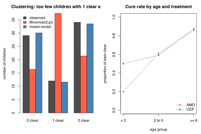
(The third bar in the left panel is the fitted distribution from the mixed model of part (b), included here so the two panels can be read together.)
(b) Random effects logistic regression. The data must first be expanded to one binary row per ear. When a child has one clear ear, which ear is labelled clear is arbitrary; since no ear-level covariate appears in the model, the two ears are exchangeable and the likelihood is unaffected by the choice. The arbitrary labelling does matter for a raw ear-by-ear correlation, however, so that is computed over both orderings of each pair.
library(lme4)
kids <- ear[rep(seq_len(nrow(ear)), ear$frequency), c("age", "treatment", "nclear")]
kids$child <- factor(seq_len(nrow(kids)))
ears <- kids[rep(seq_len(nrow(kids)), each = 2), ]
ears$ear <- rep(1:2, nrow(kids))
ears$y <- ifelse(ears$nclear == 2, 1, ifelse(ears$nclear == 0, 0, ears$ear - 1))
c(children = nrow(kids), ears = nrow(ears), cured = sum(ears$y))
E <- matrix(ears$y, nrow = 2)
round(cor(c(E[1, ], E[2, ]), c(E[2, ], E[1, ])), 3)
g1 <- glmer(y ~ age + treatment + (1 | child), data = ears, family = binomial,
control = glmerControl(optimizer = "bobyqa"))
summary(g1)
children ears cured
75 150 80
[1] 0.679
Random effects:
Groups Name Variance Std.Dev.
child (Intercept) 16.24 4.03
Number of obs: 150, groups: child, 75
Fixed effects:
Estimate Std. Error z value Pr(>|z|)
(Intercept) -3.112 1.803 -1.726 0.0843
age2 to 5 3.118 2.074 1.503 0.1328
age>= 6 7.466 3.120 2.393 0.0167
treatmentCEF 1.872 1.476 1.268 0.2049
AIC BIC logLik df.resid
169.8 184.8 -79.9 145
The estimated between-child variance is \(\hat{\sigma}_b^2 = 16.24\), giving a latent-scale intra-class correlation \(16.24/(16.24 + \pi^2/3) = 0.83\); the raw correlation between the two binary ear responses is \(0.68\). Compared with the naive glm the coefficients are all inflated by roughly a factor of three (\(0.643 \to 1.872\) for treatment, \(2.570 \to 7.466\) for age \(\geq 6\)) while the standard errors are inflated by about the same factor. This is the standard distinction between the subject-specific parameters of a mixed model and the population-averaged parameters of a marginal model: with a logit link the marginal coefficients are attenuated by approximately \((1 + 0.346\hat{\sigma}_b^2)^{-1/2} = 0.39\) here, and \(0.643/0.39 = 1.65\) is in fair agreement with \(1.872\).
g0 <- glm(y ~ age + treatment, data = ears, family = binomial)
c(logLik.glmer = as.numeric(logLik(g1)), logLik.glm = as.numeric(logLik(g0)),
LR = 2 * as.numeric(logLik(g1) - logLik(g0)))
ears$agesc <- as.numeric(ears$age)
ctl <- glmerControl(optimizer = "bobyqa")
g2 <- glmer(y ~ agesc + treatment + (1 | child), ears, binomial, control = ctl)
g3 <- glmer(y ~ age * treatment + (1 | child), ears, binomial, control = ctl)
g4 <- glmer(y ~ age + (1 | child), ears, binomial, control = ctl)
g5 <- glmer(y ~ treatment + (1 | child), ears, binomial, control = ctl)
round(AIC(g1, g2, g3, g4, g5), 2)
anova(g4, g1)
anova(g1, g3)
round(summary(g2)$coef, 4)
logLik.glmer logLik.glm LR
-79.87736 -92.31631 24.87790
df AIC
g1 5 169.75
g2 4 167.93
g3 7 170.42
g4 4 169.81
g5 3 182.62
g4: y ~ age + (1 | child)
g1: y ~ age + treatment + (1 | child)
npar AIC BIC logLik -2*log(L) Chisq Df Pr(>Chisq)
g4 4 169.81 181.86 -80.907 161.81
g1 5 169.75 184.81 -79.877 159.75 2.0587 1 0.1513
g1: y ~ age + treatment + (1 | child)
g3: y ~ age * treatment + (1 | child)
npar AIC BIC logLik -2*log(L) Chisq Df Pr(>Chisq)
g1 5 169.75 184.81 -79.877 159.75
g3 7 170.42 191.49 -78.208 156.42 3.3385 2 0.1884
Estimate Std. Error z value Pr(>|z|)
(Intercept) -7.2518 3.5524 -2.0414 0.0412
agesc 3.8529 1.7641 2.1840 0.0290
treatmentCEF 1.8137 1.5220 1.1916 0.2334
The random effect is unambiguously needed: \(\mathrm{LR} = 24.9\) against a \(\frac{1}{2}\chi^2_0 + \frac{1}{2}\chi^2_1\) null (the variance is on the boundary), \(p < 10^{-6}\). Dropping treatment costs only \(\Delta(-2\log L) = 2.06\) on 1 d.f. (\(p = 0.15\)), and the age by treatment interaction costs \(3.34\) on 2 d.f. (\(p = 0.19\)). Treating age as a linear score \(1, 2, 3\) instead of a factor loses nothing and gives the lowest AIC (167.93 versus 169.75), with \(\hat{\beta}_1 = 3.85\) per age band.
How well does the model fit? With binary responses the residual deviance is not a usable goodness-of-fit statistic, so instead compare the fitted and observed distributions of the number of clear ears per child, simulating from the fitted model:
set.seed(9418)
sim <- simulate(g1, nsim = 2000)
cnt <- sapply(sim, function(s) table(factor(colSums(matrix(s, nrow = 2)), levels = 0:2)))
rbind(observed = o, fitted.mean = round(rowMeans(cnt), 2))
round(apply(cnt, 1, quantile, c(0.025, 0.975)), 1)
0 1 2
observed 29.00 12.00 34.00
fitted.mean 30.01 11.58 33.41
0 1 2
2.5% 22 6 26
97.5% 38 18 41
The mixed model reproduces the observed \((29, 12, 34)\) almost exactly, and all three observed counts sit comfortably inside the simulated 95% intervals. This is the same comparison drawn in the left panel of the figure in part (a): the independence model predicts 37 children with one clear ear against 12 observed, the mixed model predicts 11.6. The random effect is doing exactly the job it was introduced to do.
For a population-averaged comparison, the GEE of Section 11.4 with an exchangeable working correlation:
library(geepack)
gee <- geeglm(y ~ age + treatment, id = child, data = ears[order(ears$child), ],
family = binomial, corstr = "exchangeable")
summary(gee)$coefficients
summary(gee)$corr
Estimate Std.err Wald Pr(>|W|)
(Intercept) -0.9244678 0.4070739 5.157474 0.023146540
age2 to 5 0.8670782 0.4772004 3.301527 0.069215505
age>= 6 2.5703802 0.8652488 8.824960 0.002971379
treatmentCEF 0.6424520 0.4711431 1.859412 0.172692648
Estimate Std.err
alpha 0.6005782 0.1756817
The estimates are identical to the naive glm (as they must be, since with a common cluster size and no ear-level covariate the exchangeable GEE has the same estimating equations as independence), but the sandwich standard errors are inflated by about 25%, and the treatment \(p\)-value moves from \(0.084\) to \(0.173\). With \(J = 75\) clusters this sandwich estimator is trustworthy, unlike the one in Exercise 11.1. The estimated working correlation \(\hat{\alpha} = 0.60\) agrees closely with the raw ear-to-ear correlation of \(0.68\).
Conclusion about the treatments. Age is the dominant determinant of cure: on the subject-specific scale the odds of an ear clearing multiply by \(e^{3.85} = 47\) per age band, and the observed cure rate rises from 36% under 2 to 86% at 6 or over. CEF has a higher point estimate than AMO on every scale — subject-specific odds ratio \(e^{1.87} = 6.5\), population-averaged \(e^{0.64} = 1.90\) — but the evidence is weak once clustering is accounted for (\(p = 0.15\) from the mixed model, \(0.17\) from the GEE, against a misleadingly small \(0.08\) from the naive analysis). The honest conclusion is that these data do not establish a difference between CEF and AMO; ignoring the clustering would have made the difference look about twice as convincing as it is.
(c) Nominal logistic regression on the child-level response. Rosner’s alternative treats each child as one observation with an unordered three-category response \(0, 1, 2\) clear ears, and fits the nominal model (8.4) of Chapter 8 with category 0 as the reference.
library(nnet)
ear$resp <- factor(ear$nclear, levels = 0:2)
nm <- multinom(resp ~ age + treatment, weights = frequency, data = ear, trace = FALSE)
summary(nm)$coefficients
summary(nm)$standard.errors
round(2 * (1 - pnorm(abs(summary(nm)$coefficients / summary(nm)$standard.errors))), 4)
nm0 <- multinom(resp ~ age, weights = frequency, data = ear, trace = FALSE)
anova(nm0, nm)
sat <- multinom(resp ~ age * treatment, weights = frequency, data = ear, trace = FALSE)
c(dev.model = deviance(nm), dev.saturated = deviance(sat),
GOF = deviance(nm) - deviance(sat), df = 4,
p = 1 - pchisq(deviance(nm) - deviance(sat), 4))
(Intercept) age2 to 5 age>= 6 treatmentCEF
1 -2.235765 1.186796 1.864286 1.1417153
2 -1.077013 1.065243 3.048775 0.7880926
(Intercept) age2 to 5 age>= 6 treatmentCEF
1 0.7753158 0.7599566 1.548088 0.7953606
2 0.5195994 0.5846200 1.148851 0.5775238
(Intercept) age2 to 5 age>= 6 treatmentCEF
1 0.0039 0.1184 0.2285 0.1512
2 0.0382 0.0684 0.0080 0.1724
Likelihood ratio tests of Multinomial Models
Model Resid. df Resid. Dev Test Df LR stat. Pr(Chi)
1 age 30 139.8153
2 age + treatment 28 136.8639 1 vs 2 2 2.951444 0.2286136
dev.model dev.saturated GOF df p
136.86390 131.73832 5.12558 4.00000 0.27470
The nominal model fits: the deviance difference from the saturated model (which has a free trinomial distribution in each of the six age by treatment cells) is \(5.13\) on 4 d.f., \(p = 0.27\). Treatment costs \(\mathrm{LR} = 2.95\) on 2 d.f., \(p = 0.23\) — essentially the same verdict as the mixed model’s \(p = 0.15\) and the GEE’s \(p = 0.17\), and again far weaker than the naive \(p = 0.08\). The two treatment coefficients, \(1.14\) for “1 clear versus 0” and \(0.79\) for “2 clear versus 0”, both favour CEF and are of similar size, which is a hint that the two logits could be constrained. Doing so with a proportional odds model (8.14) gives:
library(MASS)
po <- polr(resp ~ age + treatment, weights = frequency, data = ear, Hess = TRUE)
summary(po)$coefficients
c(AIC.nominal = AIC(nm), AIC.propodds = AIC(po))
Value Std. Error t value
age2 to 5 0.8896723 0.4915286 1.810011
age>= 6 2.5941220 0.8709245 2.978584
treatmentCEF 0.5715353 0.4901230 1.166106
0|1 0.5387183 0.4435641 1.214522
1|2 1.2945423 0.4655489 2.780680
AIC.nominal AIC.propodds
152.8639 149.5351
The proportional odds model has the lower AIC (\(149.5\) versus \(152.9\)) and its treatment log odds ratio \(0.572\) (s.e. \(0.490\)) is close to the GEE’s \(0.643\) (s.e. \(0.471\)) — unsurprising, since both are marginal, population-averaged summaries.
Which approach is preferable? The three approaches answer subtly different questions and the choice depends on which one is wanted.
- Assumptions.
- The nominal model of (c) is the least demanding: it assumes only that the 75 children are independent and that the trinomial cell probabilities follow a log-linear form. It makes no assumption at all about how the two ears are correlated, because the correlation is absorbed into the free category probabilities. The mixed model of (b) assumes a specific mechanism — a Normal child-level random intercept — and requires that mechanism to be right for the standard errors to be right; here the simulation check shows it is right, but that is a check that had to be done. The GEE assumes least of all about the correlation but needs many clusters for the sandwich estimator, which is satisfied with 75 children.
- Ease of computation.
- The nominal model is a one-line
multinomcall on the 18-row table as printed and needs no data expansion; the mixed model requires expanding to 150 ear-level rows, choosing an optimiser, and numerical integration over the random effect (Laplace or adaptive Gauss-Hermite). With cluster size \(K = 2\) this is easy, but the nominal approach is easier still. - Ease of interpretation.
- Here the mixed model wins. Its \(\beta_2\) is a log odds ratio for a single ear, which is what a clinician wants — “the odds that this ear clears” — and it separates the treatment effect \(\beta_2\) from the child-to-child heterogeneity \(\sigma_b^2\), which is itself informative (\(\hat{\sigma}_b^2 = 16.2\) says that whether a child’s ears clear is mostly a property of the child). The nominal model’s two coefficients per covariate are contrasts between child-level outcome categories and have no clean “per ear” reading; worse, the number of parameters doubles and there is no single treatment effect to report, only a 2 d.f. test.
- Scaling.
- The decisive practical objection to (c) is that it does not generalise. It works only because \(K = 2\) gives just three response categories. With four eyes, or teeth, or repeated measurements, the number of categories explodes and the approach becomes useless, whereas the random effects model and the GEE are unaffected.
On balance the mixed model of part (b) is preferable for reporting, with the GEE as a population-averaged cross-check; the nominal or proportional odds model of part (c) is a valuable robustness check precisely because it makes no assumption about the correlation structure, and the fact that all three give the same answer about treatment (\(p\) between \(0.15\) and \(0.23\)) is the strongest evidence available that the conclusion does not depend on the modelling choice.
Bayesian Analysis
Problem 12.1 — Reconsider Example 12.1.4 on Schistosoma japonicum.
Reconsider Example 12.1.4 on Schistosoma japonicum. In that example the parameter \(\theta\) is the proportion of a village’s population infected, the two hypotheses are \(H_0\): infection is not endemic (\(\theta \le 0.5\)) and \(H_1\): infection is endemic (\(\theta > 0.5\)), the discrete parameter space is \(\theta = 0.0, 0.1, \ldots, 1.0\), and the prior mass \(P(H_0)\) is spread uniformly over the six values \(0.0, \ldots, 0.5\) while \(P(H_1)\) is spread uniformly over the five values \(0.6, \ldots, 1.0\). The likelihood is binomial, \(y \sim \mathrm{Bin}(10, \theta)\).
a. Using Table 12.1 calculate the posterior probability for \(H_1\) for the following priors and observed data. The table to be completed has two rows, one for the prior \(P(H_1) = 0.5\) and one for the prior \(P(H_1) = 0.99\), and two columns of observed data, “5 out of 10 positive” and “1 out of 10 positive”.
b. Recalculate the above probabilities using the finer parameter space of \(\theta = 0.00, 0.01, 0.02, \ldots, 0.99, 1.00\). Explain the differences in your results. (difficulty: \(\star\star\))
The whole calculation is Equation (12.3),
\begin{equation*} P(\theta \mid y) = \frac{P(y \mid \theta)P(\theta)}{\sum_\theta P(y \mid \theta)P(\theta)}, \qquad P(H_1 \mid y) = \sum_{\theta > 0.5} P(\theta \mid y), \end{equation*}
with \(P(y \mid \theta) = \binom{10}{y}\theta^y(1-\theta)^{10-y}\) and a prior that puts mass \(P(H_1)\) uniformly on the \(\theta\)-values above \(0.5\) and mass \(1 - P(H_1)\) uniformly on those at or below \(0.5\). Only the prior mass and the grid change between the parts, so one function does everything.
postH1 <- function(theta, y, n, pH1) {
H1 <- theta > 0.5
prior <- ifelse(H1, pH1 / sum(H1), (1 - pH1) / sum(!H1))
lik <- dbinom(y, n, theta)
post <- lik * prior / sum(lik * prior)
sum(post[H1])
}
theta <- seq(0, 1, by = 0.1)
postH1(theta, 7, 10, 0.8) # reproduces the last column of Table 12.1
[1] 0.954498
That is the \(0.9545\) printed at the foot of Table 12.1, so the function is doing exactly the book’s arithmetic.
(a) The eleven-point grid. Reproducing the whole of Table 12.1 for the first new cell (prior \(P(H_1)=0.5\), data \(y = 5\)) makes the mechanism visible.
theta <- seq(0, 1, by = 0.1)
H1 <- theta > 0.5
prior <- ifelse(H1, 0.5 / 5, 0.5 / 6)
lik <- dbinom(5, 10, theta)
data.frame(theta,
hypothesis = ifelse(H1, "H1", "H0"),
prior = round(prior, 4),
likelihood = round(lik, 4),
lik.prior = round(lik * prior, 4),
posterior = round(lik * prior / sum(lik * prior), 4))
theta hypothesis prior likelihood lik.prior posterior
1 0.0 H0 0.0833 0.0000 0.0000 0.0000
2 0.1 H0 0.0833 0.0015 0.0001 0.0015
3 0.2 H0 0.0833 0.0264 0.0022 0.0271
4 0.3 H0 0.0833 0.1029 0.0086 0.1055
5 0.4 H0 0.0833 0.2007 0.0167 0.2057
6 0.5 H0 0.0833 0.2461 0.0205 0.2523
7 0.6 H1 0.1000 0.2007 0.0201 0.2469
8 0.7 H1 0.1000 0.1029 0.0103 0.1266
9 0.8 H1 0.1000 0.0264 0.0026 0.0325
10 0.9 H1 0.1000 0.0015 0.0001 0.0018
11 1.0 H1 0.1000 0.0000 0.0000 0.0000
The normalising constant is \(\sum P(y \mid \theta)P(\theta) = 0.0813\) and the \(H_1\) rows sum to \(0.4078\). Filling in all four cells:
theta <- seq(0, 1, by = 0.1)
tab <- sapply(c(5, 1), function(y)
sapply(c(0.5, 0.99), function(p) postH1(theta, y, 10, p)))
dimnames(tab) <- list(c("P(H1)=0.50", "P(H1)=0.99"), c("5 of 10", "1 of 10"))
round(tab, 4)
5 of 10 1 of 10
P(H1)=0.50 0.4078 0.0025
P(H1)=0.99 0.9855 0.1976
Read across and down. With an even-handed prior, five positives out of ten leave \(P(H_1 \mid y) = 0.408\): the data are almost exactly on the boundary between the hypotheses, so the posterior is close to the prior \(0.5\), tilted slightly towards \(H_0\) because \(\theta = 0.5\) itself is counted as part of \(H_0\) and it carries the largest likelihood in the table. One positive out of ten is strong evidence against endemicity and drives \(P(H_1 \mid y)\) to \(0.0025\).
The second row shows how much work a near-dogmatic prior does. Starting from \(P(H_1) = 0.99\), borderline data (\(y = 5\)) leave the investigator at \(0.986\) – still convinced. Even data that are flatly incompatible with endemic infection (\(y = 1\), an observed proportion of \(0.1\)) only pull her down to \(0.198\). A prior odds of \(99:1\) takes a great deal of evidence to overturn, which is the point made in Section 12.2: the further \(P(H_1)/P(H_0)\) moves from \(1\), the more the posterior is the prior’s creature rather than the data’s.
(b) The 101-point grid. Now \(\theta = 0.00, 0.01, \ldots, 1.00\), so \(H_0\) occupies \(51\) grid points and \(H_1\) occupies \(50\); the prior mass per point changes accordingly, but the total mass on each hypothesis is unchanged.
fine <- seq(0, 1, by = 0.01)
tab2 <- sapply(c(5, 1), function(y)
sapply(c(0.5, 0.99), function(p) postH1(fine, y, 10, p)))
dimnames(tab2) <- list(c("P(H1)=0.50", "P(H1)=0.99"), c("5 of 10", "1 of 10"))
round(tab2, 4)
5 of 10 1 of 10
P(H1)=0.50 0.4914 0.0054
P(H1)=0.99 0.9897 0.3516
Every entry has moved up. The reason is that Equation (12.3) with a discrete grid is a Riemann sum standing in for the integral in the continuous version of Bayes’ theorem; the grid is a numerical quadrature rule, and \(\Delta\theta = 0.1\) is a coarse one. Two explanations suggest themselves, and it is worth checking which one actually operates.
The first is that the coarse grid mislocates mass near the boundary. With \(y = 5\) the likelihood peaks at \(\theta = 0.5\), which the grid assigns wholly to \(H_0\); the interval \((0.5, 0.6)\) – which belongs to \(H_1\) and where the likelihood is nearly as large – has no grid point of its own and is effectively annexed by \(\theta = 0.5\). The same thing happens for \(y = 1\): the \(H_1\) likelihood is largest just above the boundary, \(P(y \mid 0.51) = 0.0083\) against \(P(y \mid 0.6) = 0.0016\), so the coarse grid’s leftmost \(H_1\) point understates the hypothesis by a factor of five.
The second is that the coarse grid wastes prior mass on impossible values: for \(y = 1\) both \(\theta = 0.0\) and \(\theta = 1.0\) carry likelihood exactly zero, yet \(\theta = 1.0\) holds a full fifth of the \(H_1\) prior while \(\theta = 0.0\) holds a full sixth of the \(H_0\) prior. This looks like a bias against \(H_1\), but \(1/5\) and \(1/6\) are close enough that the two losses very nearly cancel. The two explanations can be separated cleanly, because with prior mass spread uniformly within each hypothesis the whole calculation collapses to a single ratio,
\begin{equation*} P(H_1 \mid y) = \frac{P(H_1)\,B}{P(H_1)\,B + 1 - P(H_1)}, \qquad B = \frac{\overline{P(y \mid \theta)}_{H_1}}{\overline{P(y \mid \theta)}_{H_0}}, \end{equation*}
where each average is taken over that hypothesis’s grid points. The grid enters only through \(B\).
gridBF <- function(theta, y, n) {
H1 <- theta > 0.5
mean(dbinom(y, n, theta[H1])) / mean(dbinom(y, n, theta[!H1]))
}
co <- seq(0, 1, by = 0.1)
fi <- seq(0, 1, by = 0.01)
bf <- rbind("11-point grid" = sapply(c(5, 1), function(y) gridBF(co, y, 10)),
"11-point, ends cut" = sapply(c(5, 1), function(y) gridBF(co[co > 0 & co < 1], y, 10)),
"101-point grid" = sapply(c(5, 1), function(y) gridBF(fi, y, 10)))
colnames(bf) <- c("y = 5", "y = 1")
signif(bf, 4)
y = 5 y = 1
11-point grid 0.6887 0.002488
11-point, ends cut 0.7174 0.002592
101-point grid 0.9662 0.005478
The verdict is decisive. Deleting the two dead end points barely moves \(B\) – from \(0.00249\) to \(0.00259\) for \(y = 1\), and from \(0.689\) to \(0.717\) for \(y = 5\) – so the second explanation accounts for almost none of the change. Refining the grid moves \(B\) to \(0.00548\) and \(0.966\). The whole effect is the first one: the coarse grid simply has no point in the region just above \(\theta = 0.5\) where the \(H_1\) likelihood does most of its work.
The same identity explains why the \(P(H_1) = 0.99\) row moves so much further than the \(P(H_1) = 0.50\) row when \(y = 1\). Posterior odds are prior odds times \(B\), and \(B\) roughly doubles under refinement in both rows. With prior odds \(1:1\) that turns posterior odds of \(0.0025\) into \(0.0055\), which as a probability is a move from \(0.0025\) to \(0.0054\) – invisible. With prior odds \(99:1\) the same doubling turns posterior odds of \(0.246\) into \(0.542\), a move from \(0.198\) to \(0.352\). The quadrature error is identical; only the leverage differs, because a probability near \(0.2\) is far more sensitive to a change in odds than one near \(0.003\).
The diagnosis is confirmed by driving the grid to the continuum. With a uniform prior over \([0,1]\) (which is the \(P(H_1) = 0.5\) row in the limit, since the two hypotheses then have equal length) the exact posterior is \(\mathrm{Be}(y+1, n-y+1)\) by Equation (12.6), so \(P(H_1 \mid y) = 1 - F_{\mathrm{Be}}(0.5)\) can be written down in closed form.
c(exact_y5 = 1 - pbeta(0.5, 5 + 1, 10 - 5 + 1),
exact_y1 = 1 - pbeta(0.5, 1 + 1, 10 - 1 + 1))
for (k in c(10, 100, 1000, 10000))
cat(sprintf("step %8.5f y=5: %.4f y=1: %.4f\n", 1 / k,
postH1(seq(0, 1, length = k + 1), 5, 10, 0.5),
postH1(seq(0, 1, length = k + 1), 1, 10, 0.5)))
exact_y5 exact_y1
0.500000000 0.005859375
step 0.10000 y=5: 0.4078 y=1: 0.0025
step 0.01000 y=5: 0.4914 y=1: 0.0054
step 0.00100 y=5: 0.4991 y=1: 0.0058
step 0.00010 y=5: 0.4999 y=1: 0.0059
The grid answers converge to \(0.5\) and \(0.005859\), and the \(101\)-point values are already within about \(0.01\) and \(0.0005\) of the truth. So the fine grid is not giving different answers because of any change of belief; it is giving less biased answers to the same question. The price is the one flagged in Section 12.1.4 – Table 12.1 grows from \(11\) rows to \(101\), and in a model with \(m\) parameters the same refinement multiplies the work by \(10^m\). That cost is precisely the motivation for the simulation methods of Chapter 13.
Problem 12.2 — Show that the posterior distribution using a Normally distributed prior
Show that the posterior distribution using a Normally distributed prior \(\mathrm{N}(\mu_0, \sigma_0^2)\) and Normally distributed likelihood \(\mathrm{N}(\mu_l, \sigma_l^2)\) is also Normally distributed with mean
\begin{equation*} \frac{\mu_0\sigma_l^2 + \mu_l\sigma_0^2}{\sigma_0^2 + \sigma_l^2} \end{equation*}
and variance
\begin{equation*} \frac{\sigma_l^2\sigma_0^2}{\sigma_0^2 + \sigma_l^2}. \end{equation*}
(difficulty: \(\star\star\))
This is the conjugacy claim made in Section 12.2.2 and used there to obtain the sceptical posterior. It is a completion of the square, and the whole argument can be carried out with proportionality because Equation (12.2), \(P(\theta \mid \mathbf{y}) \propto P(\mathbf{y} \mid \theta)P(\theta)\), only ever determines the posterior up to the normalising constant.
Let \(\theta\) be the parameter – the log hazard ratio in the example. The prior is
\begin{equation*} P(\theta) = \frac{1}{\sigma_0\sqrt{2\pi}}\exp\!\left(-\frac{(\theta - \mu_0)^2}{2\sigma_0^2}\right), \end{equation*}
and the likelihood, regarded as a function of \(\theta\), is
\begin{equation*} P(\mathbf{y} \mid \theta) = \frac{1}{\sigma_l\sqrt{2\pi}}\exp\!\left(-\frac{(\mu_l - \theta)^2}{2\sigma_l^2}\right), \end{equation*}
where \(\mu_l\) is the observed summary (the maximum likelihood estimate) and \(\sigma_l^2\) its sampling variance, both treated as known. Note that \((\mu_l - \theta)^2 = (\theta - \mu_l)^2\), so the likelihood is a Normal kernel in \(\theta\) centred at \(\mu_l\); this is what allows the two exponents to be combined.
Multiplying and discarding every factor free of \(\theta\),
\begin{equation*} P(\theta \mid \mathbf{y}) \;\propto\; \exp\!\left(-\tfrac{1}{2}Q(\theta)\right), \qquad Q(\theta) = \frac{(\theta - \mu_0)^2}{\sigma_0^2} + \frac{(\theta - \mu_l)^2}{\sigma_l^2}. \end{equation*}
Expanding \(Q\) and collecting powers of \(\theta\),
\begin{equation*} Q(\theta) = \theta^2\left(\frac{1}{\sigma_0^2} + \frac{1}{\sigma_l^2}\right)
- 2\theta\left(\frac{\mu_0}{\sigma_0^2} + \frac{\mu_l}{\sigma_l^2}\right)
- \left(\frac{\mu_0^2}{\sigma_0^2} + \frac{\mu_l^2}{\sigma_l^2}\right). \end{equation*}
The quadratic coefficient is the sum of the two precisions. Define
\begin{equation*} \frac{1}{\sigma_p^2} = \frac{1}{\sigma_0^2} + \frac{1}{\sigma_l^2} = \frac{\sigma_0^2 + \sigma_l^2}{\sigma_0^2\sigma_l^2}, \qquad\text{so}\qquad \sigma_p^2 = \frac{\sigma_l^2\sigma_0^2}{\sigma_0^2 + \sigma_l^2}, \end{equation*}
which is already the required variance, and define
\begin{equation*} \mu_p = \sigma_p^2\left(\frac{\mu_0}{\sigma_0^2} + \frac{\mu_l}{\sigma_l^2}\right) = \frac{\sigma_0^2\sigma_l^2}{\sigma_0^2 + \sigma_l^2}\cdot\frac{\mu_0\sigma_l^2 + \mu_l\sigma_0^2}{\sigma_0^2\sigma_l^2} = \frac{\mu_0\sigma_l^2 + \mu_l\sigma_0^2}{\sigma_0^2 + \sigma_l^2}, \end{equation*}
which is the required mean. With these two definitions,
\begin{equation*} Q(\theta) = \frac{\theta^2 - 2\theta\mu_p}{\sigma_p^2} + c_1 = \frac{(\theta - \mu_p)^2}{\sigma_p^2} + c_2 , \end{equation*}
where \(c_1\) and \(c_2\) collect terms free of \(\theta\) (specifically \(c_2 = c_1 - \mu_p^2/\sigma_p^2\)). Since \(\exp(-c_2/2)\) is a constant it is absorbed into the proportionality, leaving
\begin{equation*} P(\theta \mid \mathbf{y}) \;\propto\; \exp\!\left(-\frac{(\theta - \mu_p)^2}{2\sigma_p^2}\right). \end{equation*}
A density proportional to this kernel must be the \(\mathrm{N}(\mu_p, \sigma_p^2)\) density, because the kernel integrates to \(\sigma_p\sqrt{2\pi}\) over \((-\infty, \infty)\) and the constant of proportionality is fixed by \(\int P(\theta \mid \mathbf{y})\,d\theta = 1\). Hence
\begin{equation*} \theta \mid \mathbf{y} \;\sim\; \mathrm{N}\!\left(\frac{\mu_0\sigma_l^2 + \mu_l\sigma_0^2}{\sigma_0^2 + \sigma_l^2},\; \frac{\sigma_l^2\sigma_0^2}{\sigma_0^2 + \sigma_l^2}\right), \end{equation*}
as required. The Normal family is therefore conjugate to a Normal likelihood with known variance, in the sense defined in Section 12.2.2 – exactly as the Beta family is conjugate to Binomial data in Equation (12.6).
Three features are worth naming, because they are what makes the result useful.
Precisions add: \(1/\sigma_p^2 = 1/\sigma_0^2 + 1/\sigma_l^2\). The posterior is therefore always more precise than either the prior or the likelihood alone, and \(\sigma_p^2 < \min(\sigma_0^2, \sigma_l^2)\).
The posterior mean is a precision-weighted average of the two inputs,
\begin{equation*} \mu_p = \frac{\sigma_0^{-2}}{\sigma_0^{-2} + \sigma_l^{-2}}\,\mu_0 + \frac{\sigma_l^{-2}}{\sigma_0^{-2} + \sigma_l^{-2}}\,\mu_l , \end{equation*}
so it always lies between \(\mu_0\) and \(\mu_l\) – which is why the sceptical posterior in Figure 12.1 sits between the sceptical prior and the likelihood. The weights are the relative precisions, so the more confident source wins.
A flat prior is the limit \(\sigma_0^2 \to \infty\), under which \(\mu_p \to \mu_l\) and \(\sigma_p^2 \to \sigma_l^2\): the posterior collapses onto the likelihood. That is the uninformative-prior panel on the right of Figure 12.1, where prior and posterior coincide and the Bayesian answer reproduces the frequentist one.
As a check that the formulae are the ones the book actually used, feed in the sceptical prior \(\mathrm{N}(0, 0.1907^2)\) and the trial likelihood \(\mathrm{N}(0.580, 0.2266^2)\) from Section 12.2.2, which reports a posterior mean of \(0.240\) and a posterior probability of \(0.31\) that the improvement exceeds \(10\%\) (that is, \(\mathrm{LHR} > 0.3137\)).
mu0 <- 0; s0 <- 0.1907 # sceptical prior, Section 12.2.2
mul <- 0.580; sl <- 0.2266 # observed LHR and its standard error
mup <- (mu0 * sl^2 + mul * s0^2) / (s0^2 + sl^2)
sp <- sqrt(sl^2 * s0^2 / (s0^2 + sl^2))
c(post_mean = mup, post_sd = sp, P_improvement_over_10pct = 1 - pnorm(0.3137, mup, sp))
post_mean post_sd P_improvement_over_10pct
0.2404696 0.1459070 0.3078697
Both printed values are recovered, so the analytic result agrees with the numerical integration the book performed for illustration – and it does so without ever needing the normalising constant \(c\) that appears in the displayed expression for \(P(\mathbf{y} \mid \theta)P(\theta)\) in Section 12.2.2.
Problem 12.3 — Reconsider Example 12.2.2 about the cancer clinical trial. The 11 special-
Reconsider Example 12.2.2 about the cancer clinical trial. The 11 specialists taking part in the trial had an enthusiastic prior opinion that the median expected improvement in survival was 10%, which corresponds to an LHR of 0.3137. Assume that their prior opinion can be represented as a Normal distribution with a mean of 0.3137 and a standard deviation of 0.1907 (as per the sceptics’ prior).
a. What is their prior probability that the new treatment is effective?
b. What is their posterior probability that the new treatment is effective? (difficulty: \(\star\))
Everything is on the log-hazard-ratio scale of Equation (12.4),
\begin{equation*} \mathrm{LHR} = \log\!\left(\frac{H_1}{H_2}\right) = \log\!\left(\frac{-\log P_1}{-\log P_2}\right), \end{equation*}
where \(P_1 = 0.15\) is two-year survival on conventional therapy and \(P_2\) is two-year survival on the new treatment. The new treatment is effective exactly when its hazard is lower, that is when \(H_2 < H_1\), that is when \(\theta = \mathrm{LHR} > 0\). So both parts ask for \(P(\theta > 0)\), first under the prior and then under the posterior.
The enthusiastic prior is \(\theta \sim \mathrm{N}(0.3137,\, 0.1907^2)\) and the trial data of Section 12.2.2 – 78 deaths among 256 patients – give the likelihood \(\mathrm{N}(0.580,\, 0.2266^2)\), the standard deviation coming from the reported 95% confidence interval \(0.580 \pm 0.444\).
(a) Prior probability of effectiveness.
\begin{equation*} P(\theta > 0) = 1 - \Phi\!\left(\frac{0 - 0.3137}{0.1907}\right) = \Phi(1.6449) = 0.950 . \end{equation*}
mu0 <- 0.3137; s0 <- 0.1907 # enthusiastic prior
1 - pnorm(0, mu0, s0) # prior P(LHR > 0)
[1] 0.9500143
The answer is \(0.95\), and it is \(0.95\) by construction rather than by coincidence. The standard deviation \(0.1907\) was chosen in Section 12.2.2 so that \(1.645\sigma = 0.3137\); borrowing it for a distribution centred at \(0.3137\) puts zero exactly \(1.645\) standard deviations below the mean. The two priors are mirror images about the halfway point \(\mathrm{LHR} = 0.157\): the sceptics put probability \(0.05\) on an improvement exceeding 10%, and the enthusiasts put probability \(0.05\) on the treatment being no better than conventional therapy. That is a strong opinion – before seeing a single patient the specialists give \(19:1\) odds that the new treatment helps.
(b) Posterior probability of effectiveness. By Exercise 12.2 the posterior is Normal with
\begin{equation*} \mu_p = \frac{\mu_0\sigma_l^2 + \mu_l\sigma_0^2}{\sigma_0^2 + \sigma_l^2}, \qquad \sigma_p^2 = \frac{\sigma_l^2\sigma_0^2}{\sigma_0^2 + \sigma_l^2}, \end{equation*}
so no numerical integration is needed.
mul <- 0.580; sl <- 0.2266 # likelihood: observed LHR and its standard error
mup <- (mu0 * sl^2 + mul * s0^2) / (s0^2 + sl^2)
sp <- sqrt(sl^2 * s0^2 / (s0^2 + sl^2))
c(post_mean = mup, post_sd = sp,
P_effective = 1 - pnorm(0, mup, sp),
P_over_10pct = 1 - pnorm(0.3137, mup, sp),
abs_improvement = 0.15^exp(-mup) - 0.15)
post_mean post_sd P_effective P_over_10pct abs_improvement
0.4241087 0.1459070 0.9981737 0.7753871 0.1389835
The posterior is \(\mathrm{N}(0.424,\, 0.146^2)\) and the posterior probability that the new treatment is effective is
\begin{equation*} P(\theta > 0 \mid \mathbf{y}) = 1 - \Phi\!\left(\frac{-0.4241}{0.1459}\right) = \Phi(2.907) = 0.998 . \end{equation*}
th <- seq(-1.15, 1.15, length = 500)
plot(th, dnorm(th, mup, sp), type = "l", lwd = 2, ylim = c(0, 3), xlab = "log hazard ratio",
ylab = "density", main = "Enthusiastic prior, likelihood and posterior")
lines(th, dnorm(th, mu0, s0), lty = 2, lwd = 2)
lines(th, dnorm(th, mul, sl), lty = 3, lwd = 2)
abline(v = c(0, 0.3137), col = "grey60")
legend("topleft", c("posterior", "enthusiastic prior", "likelihood"), lty = 1:3, lwd = 2, bty = "n")
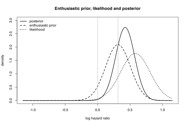
Interpretation, and the contrast that is the point of the exercise. The posterior mean \(0.424\) sits between the prior mean \(0.3137\) and the observed \(0.580\), as Exercise 12.2 guarantees, and slightly nearer the prior because the prior is the more precise of the two (\(0.1907 < 0.2266\)). On the survival scale \(\mathrm{LHR} = 0.424\) corresponds to \(P_2 = 0.15^{\exp(-0.424)} = 0.289\), an absolute improvement of about 14 percentage points – between the enthusiasts’ prior median of 10% and the trial’s own 20%.
Set this beside the sceptical analysis in Section 12.2.2. The same data, run through the sceptical prior \(\mathrm{N}(0, 0.1907^2)\), give a posterior mean of \(0.240\), a probability of only \(0.31\) that the improvement exceeds 10%, and a probability \(0.95\) that the treatment is effective at all. Through the enthusiastic prior they give \(0.775\) and \(0.998\). Both groups saw one trial; the sceptics come away thinking the treatment probably works but not by enough to change practice, while the enthusiasts come away all but certain and with better than three-to-one odds on a clinically worthwhile gain. The trial has moved the enthusiasts from \(0.95\) to \(0.998\) – a small movement in probability, but the odds on effectiveness have risen from \(19:1\) to \(546:1\).
This is the honest cost of informative priors, and it is why Section 12.2.1 recommends always reporting the uninformative-prior result alongside. Under a flat prior the posterior is the likelihood, giving \(P(\theta > 0 \mid \mathbf{y}) = 1 - \Phi(-0.580/0.2266) = 0.9948\) and \(P(\theta > 0.3137 \mid \mathbf{y}) = 0.880\); these are the uninformative-prior figures quoted at the end of Section 12.2.2, where they are rounded to \(0.99\) and \(0.88\). A reader starting from neutrality lands much closer to the enthusiasts than to the sceptics here, which tells us the enthusiastic prior is not doing violence to the data – but it is the neutral analysis, not either partisan one, that lets a third party judge that for themselves.
Problem 12.4 — Reconsider Example 12.2.3 on overdoses among released prisoners. You
Reconsider Example 12.2.3 on overdoses among released prisoners, in which none of the \(n = 91\) contactable released prisoners had overdosed in the four weeks after release. You may find the First Bayes software useful for answering these questions.
a. Use an argument based on \(\alpha - 1\) previous successes and \(\beta - 1\) previous failures to calculate a heuristic Beta prior. Combine this prior with the data to give a Beta posterior.
b. Calculate the mean of the posterior. Compare this mean to the investigator’s prior opinion of 1 overdose in 200 subjects (0.005). Considering that there were no overdoses in the data, what is wrong with this posterior? (difficulty: \(\star\star\))
(a) The heuristic prior and the resulting posterior. Section 12.2.3 gives the heuristic: a \(\mathrm{Be}(\alpha, \beta)\) prior behaves as though one had already observed \(\alpha - 1\) successes and \(\beta - 1\) failures. The chief investigator’s opinion is one overdose per 200 released prisoners, so the pseudo-data are 1 prior “success” (an overdose) and \(200 - 1 = 199\) prior “failures”. Reading the heuristic backwards,
\begin{equation*} \alpha - 1 = 1 \;\Rightarrow\; \alpha = 2, \qquad \beta - 1 = 199 \;\Rightarrow\; \beta = 200, \end{equation*}
so the heuristic prior is \(\theta \sim \mathrm{Be}(2, 200)\).
Combining with the data through Equation (12.6), \(P(\theta \mid \mathbf{y}) \sim \mathrm{Be}(y + \alpha,\, n - y + \beta)\) with \(n = 91\) and \(y = 0\):
\begin{equation*} \theta \mid \mathbf{y} \;\sim\; \mathrm{Be}(0 + 2,\; 91 - 0 + 200) = \mathrm{Be}(2, 291). \end{equation*}
a0 <- 2; b0 <- 200 # 1 prior overdose, 199 prior non-overdoses
n <- 91; y <- 0 # 91 contactable prisoners, no overdoses
a1 <- y + a0; b1 <- n - y + b0
c(prior_mean = a0/(a0 + b0), prior_mode = (a0 - 1)/(a0 + b0 - 2),
post_alpha = a1, post_beta = b1)
prior_mean prior_mode post_alpha post_beta
9.90099e-03 5.00000e-03 2.00000e+00 2.91000e+02
The first two numbers already contain the answer to part (b), so keep them in view: the prior mode is exactly \(1/200 = 0.005\), but the prior mean is \(2/202 = 0.0099\), nearly twice the investigator’s stated opinion.
(b) The posterior mean, and what is wrong with it. From Exercise 7.5, \(\mathrm{E}(\theta) = \alpha/(\alpha + \beta)\) for \(\theta \sim \mathrm{Be}(\alpha, \beta)\), so the posterior mean is \(2/293\).
c(post_mean = a1/(a1 + b1), post_mode = (a1 - 1)/(a1 + b1 - 2),
lower = qbeta(0.025, a1, b1), upper = qbeta(0.975, a1, b1),
investigator_prior_mean = 0.005)
post_mean post_mode lower
0.0068259386 0.0034364261 0.0008305628
upper investigator_prior_mean
0.0189322698 0.0050000000
The posterior mean is \(\widehat{\theta} = 2/293 = 0.00683\), or about 1 overdose in 147 released prisoners, with a 95% posterior interval of \((0.00083,\, 0.0189)\).
What is wrong is immediate once it is stated in those terms. The investigator went in believing the rate was 1 in 200; she then followed 91 prisoners and saw no overdoses at all, which is evidence that the rate is at or below her prior guess, never above it. Yet the posterior mean \(0.0068\) is larger than the prior opinion \(0.005\). Evidence of no events has apparently pushed the estimated risk up by more than a third. No coherent updating rule can do that, so the fault must lie in the prior rather than in Bayes’ theorem.
It does. The culprit is the heuristic itself, and Section 12.2.3 flags it in passing – “although this is only true for relatively large values of \(\alpha\) and \(\beta\)”. The pseudo-count reading matches the mode of the Beta distribution,
\begin{equation*} \mathrm{mode} = \frac{\alpha - 1}{\alpha + \beta - 2} = \frac{1}{200} = 0.005, \end{equation*}
not the mean, and for a Beta density this skewed the two are far apart. The prior actually elicited is \(\mathrm{Be}(2, 200)\), whose mean is \(2/202 = 0.0099\). So the analysis never encoded “1 in 200” as an expected rate at all; it encoded “1 in 101” and merely made 1 in 200 the single most likely value. Bayes’ theorem then did its job faithfully: the mean fell from \(0.0099\) to \(0.0068\), a genuine downward move in response to the zero count. The comparison with \(0.005\) is a comparison against a number the prior never represented.
The fix is to match the prior to the moment the investigator actually stated. Setting \(\alpha/(\alpha + \beta) = 1/200\) with \(\alpha = 1\) gives \(\mathrm{Be}(1, 199)\), which is what Table 12.2 uses, and the posterior is then \(\mathrm{Be}(1, 290)\) with mean \(1/291 = 0.00344\) – comfortably below \(0.005\), as observing no overdoses demands.
rbind("Be(2,200) heuristic" = c(prior = 2/202, posterior = 2/293),
"Be(1,199) book, Table 12.2" = c(prior = 1/200, posterior = 1/291))
prior posterior
Be(2,200) heuristic 0.00990099 0.006825939
Be(1,199) book, Table 12.2 0.00500000 0.003436426
A neat consistency check: the mode of the heuristic posterior \(\mathrm{Be}(2, 291)\) is \(1/291 = 0.003436\), numerically identical to the mean of the book’s posterior \(\mathrm{Be}(1, 290)\). This is not an accident of the numbers. The heuristic route always produces \(\mathrm{Be}(y + 2,\, n - y + 200)\), whose mode is \((y+1)/(n+200)\), while the book’s route produces \(\mathrm{Be}(y + 1,\, n - y + 199)\), whose mean is also \((y+1)/(n+200)\). The single extra unit of \(\alpha\) that the pseudo-count heuristic supplies is precisely what converts a mean into a mode.
p <- seq(0, 0.05, length = 500)
plot(p, dbeta(p, a1, b1), type = "l", lwd = 2, ylim = c(0, 300),
xlab = "probability of overdose", ylab = "density",
main = "Heuristic Beta prior and posterior, overdose example")
lines(p, dbeta(p, a0, b0), lty = 2, lwd = 2)
lines(p, dbeta(p, 1, 290), lty = 3, lwd = 2)
abline(v = c(0.005, a1/(a1 + b1)), col = c("grey60", "grey30"))
legend("topright", c("posterior Be(2,291)", "heuristic prior Be(2,200)",
"book posterior Be(1,290)"), lty = 1:3, lwd = 2, bty = "n")
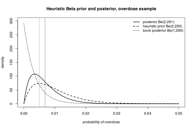
The figure shows the mechanism, and it shows how different the two shapes are. The heuristic posterior \(\mathrm{Be}(2, 291)\) (solid) rises from zero at \(\theta = 0\) to an interior mode at \(0.0034\) and then decays with a long right tail; it is that tail alone which drags the mean out to \(0.0068\), the darker vertical line, past the investigator’s \(0.005\) at the grey line. The book’s posterior \(\mathrm{Be}(1, 290)\) (dotted) has \(\alpha = 1\) and so is monotone decreasing with no interior mode whatever – its density is largest at \(\theta = 0\), at the top left of the plot, and falls away from there – yet its mean is the solid curve’s mode. That is the whole content of the discrepancy: one unit of \(\alpha\) is the difference between a density that says “zero overdoses is the single most likely rate” and one that says “\(0.0034\) is”.
Two general lessons follow, both of which matter well beyond this example. First, with a strongly skewed posterior the mean is a poor summary; the mode, median, or the whole 95% interval carries the message better, and the book reports intervals in Table 12.2 for exactly this reason. Second, elicitation must state which functional of the prior the expert’s number is – mean, median, or mode – because for small \(\alpha\) the Beta pseudo-count heuristic silently answers “mode” while the analyst reads “mean”. The prior here is doing what Section 12.2.3 said it was for, namely keeping \(0 < \widehat{\theta} < 1\) and \(\mathrm{var}(\widehat{\theta}) > 0\) in the face of a zero numerator, but a prior chosen to fix one defect can introduce another if its parameters are set by a rule of thumb outside the range where the rule is accurate.
Markov Chain Monte Carlo Methods
Problem 13.1 — Reconsider the example on Schistosoma japonicum from the previous
Reconsider the example on Schistosoma japonicum from the previous chapter (Section 12.1.4). In Table 12.1 the posterior probability for \(H_0\) was calculated using an equally spaced set of values for \(\theta\). Recalculate the values in Table 12.1 using 11 values for \(\theta\) generated from the Uniform distribution \(\mathrm{U}[0,1]\). Compare the results obtained using the fixed and random values for \(\theta\). Should any restrictions be placed on the samples generated from the Uniform distribution?
For reference, the setting is: \(\theta\) is the prevalence of infection in a village, \(H_0: \theta \le 0.5\) (not endemic) and \(H_1: \theta > 0.5\) (endemic); the investigator’s prior gives \(\Pr(H_0) = 0.2\) and \(\Pr(H_1) = 0.8\), spread uniformly over the parameter values in each region; and the data are \(y = 7\) positive stool samples out of \(n = 10\), so the likelihood is \(P(y \mid \theta) = \binom{10}{7}\theta^7(1-\theta)^3\). In Table 12.1 the eleven values \(\theta = 0.0, 0.1, \ldots, 1.0\) are used, giving prior \(0.2/6 = 0.0333\) to each of the six values with \(\theta \le 0.5\) and \(0.8/5 = 0.1600\) to each of the five values with \(\theta > 0.5\); the resulting posterior is \(P(H_0 \mid y) = 0.0455\), \(P(H_1 \mid y) = 0.9545\). (difficulty: \(\star\))
Reproducing Table 12.1. The posterior is Equation (12.3) evaluated on the grid,
\begin{equation*} P(\theta_k \mid y) = \frac{P(y \mid \theta_k)P(\theta_k)}{\sum_{j} P(y \mid \theta_j)P(\theta_j)} , \end{equation*}
and \(P(H_0 \mid y)\) is the sum of the posterior column over the rows with \(\theta \le 0.5\).
lik <- function(th) dbinom(7, 10, th)
th <- seq(0, 1, by = 0.1)
H0 <- th <= 0.5
pri <- ifelse(H0, 0.2 / sum(H0), 0.8 / sum(!H0))
lp <- lik(th) * pri
post <- lp / sum(lp)
data.frame(theta = th, hyp = ifelse(H0, "H0", "H1"), prior = round(pri, 4),
lik = round(lik(th), 4), lik.x.prior = round(lp, 4),
posterior = round(post, 4))
c(P.H0 = sum(post[H0]), P.H1 = sum(post[!H0]))
theta hyp prior lik lik.x.prior posterior
1 0.0 H0 0.0333 0.0000 0.0000 0.0000
2 0.1 H0 0.0333 0.0000 0.0000 0.0000
3 0.2 H0 0.0333 0.0008 0.0000 0.0002
4 0.3 H0 0.0333 0.0090 0.0003 0.0024
5 0.4 H0 0.0333 0.0425 0.0014 0.0114
6 0.5 H0 0.0333 0.1172 0.0039 0.0315
7 0.6 H1 0.1600 0.2150 0.0344 0.2771
8 0.7 H1 0.1600 0.2668 0.0427 0.3439
9 0.8 H1 0.1600 0.2013 0.0322 0.2595
10 0.9 H1 0.1600 0.0574 0.0092 0.0740
11 1.0 H1 0.1600 0.0000 0.0000 0.0000
P.H0 P.H1
0.04550201 0.95449799
This is Table 12.1 exactly, and it fixes the arithmetic that the random version has to imitate.
The target the grid is approximating. The grid is a crude quadrature rule for the continuous problem in which the prior is the step density
\begin{equation*} p(\theta) = \begin{cases} 0.2/0.5 = 0.4, & 0 \le \theta \le 0.5, \\ 0.8/0.5 = 1.6, & 0.5 < \theta \le 1,\end{cases} \end{equation*}
so that
\begin{equation*} P(H_1 \mid y) = \frac{1.6\int_{0.5}^{1}\theta^7(1-\theta)^3\,d\theta}{0.4\int_{0}^{0.5}\theta^7(1-\theta)^3\,d\theta + 1.6\int_{0.5}^{1}\theta^7(1-\theta)^3\,d\theta} . \end{equation*}
Both integrals are incomplete beta functions, so the exact answer is available in closed form.
I0 <- pbeta(0.5, 8, 4) * beta(8, 4)
I1 <- (1 - pbeta(0.5, 8, 4)) * beta(8, 4)
exact <- 1.6 * I1 / (0.4 * I0 + 1.6 * I1)
exact
0.9690502
The grid answer \(0.9545\) is already \(0.015\) below the truth, because the eleven equally spaced points include \(\theta = 0\) and \(\theta = 1\), where the likelihood is exactly zero. Two of the eleven evaluations are wasted, and both wasted points sit in the tails, which is why the grid understates \(P(H_1 \mid y)\).
Recalculating with 11 random values. Replace the grid by \(\theta_1, \ldots, \theta_{11} \sim \mathrm{U}[0,1]\) and keep the prior structure: whichever \(m\) of the draws land in \([0, 0.5]\) share the prior mass \(0.2\), and the remaining \(11 - m\) share \(0.8\). This is stratified Monte Carlo integration, and it preserves the investigator’s stated prior probabilities exactly.
set.seed(13001)
th <- sort(runif(11))
H0 <- th <= 0.5
pri <- ifelse(H0, 0.2 / sum(H0), 0.8 / sum(!H0))
lp <- lik(th) * pri
post <- lp / sum(lp)
data.frame(theta = round(th, 4), hyp = ifelse(H0, "H0", "H1"),
prior = round(pri, 4), lik = round(lik(th), 4),
lik.x.prior = round(lp, 4), posterior = round(post, 4))
c(P.H0 = sum(post[H0]), P.H1 = sum(post[!H0]))
theta hyp prior lik lik.x.prior posterior
1 0.0550 H0 0.0333 0.0000 0.0000 0.0000
2 0.1874 H0 0.0333 0.0005 0.0000 0.0001
3 0.3533 H0 0.0333 0.0223 0.0007 0.0058
4 0.4269 H0 0.0333 0.0584 0.0019 0.0151
5 0.4473 H0 0.0333 0.0726 0.0024 0.0188
6 0.4867 H0 0.0333 0.1050 0.0035 0.0272
7 0.7255 H1 0.1600 0.2626 0.0420 0.3266
8 0.7736 H1 0.1600 0.2309 0.0369 0.2871
9 0.8055 H1 0.1600 0.1943 0.0311 0.2416
10 0.8968 H1 0.1600 0.0615 0.0098 0.0765
11 0.9794 H1 0.1600 0.0009 0.0001 0.0011
P.H0 P.H1
0.06704378 0.93295622
This particular sample happened to split 6/5 between the hypotheses, so the prior column is identical to Table 12.1. The posterior for \(H_1\) comes out at \(0.933\) rather than \(0.9545\): the same qualitative conclusion (the prior for \(H_1\) has been reinforced by the data), but a numerically different answer, and one that no longer clears the \(0.95\) threshold the investigator used to stop testing.
One sample is not a comparison. The random answer is itself random, so the honest comparison is between the fixed number \(0.9545\) and the whole sampling distribution of the random estimator. Repeating the 11-point calculation 10,000 times:
set.seed(13002)
sim <- replicate(10000, {
th <- runif(11); H0 <- th <= 0.5; m <- sum(H0)
if (m == 0 || m == 11) return(NA_real_)
pri <- ifelse(H0, 0.2 / m, 0.8 / (11 - m))
lp <- lik(th) * pri
sum(lp[!H0]) / sum(lp)
})
c(failures = sum(is.na(sim)), mean = mean(sim, na.rm = TRUE),
sd = sd(sim, na.rm = TRUE), quantile(sim, c(0.025, 0.975), na.rm = TRUE))
mean(sim < 0.95, na.rm = TRUE)
failures mean sd 2.5% 97.5%
4.00000000 0.96615023 0.03463462 0.90303777 0.99936818
[1] 0.2031813
hist(sim, breaks = 60, col = 'grey85', border = 'white',
xlab = 'P(H1 | y) from 11 random theta', main = '', xlim = c(0.80, 1.0))
abline(v = 0.954498, col = 'blue', lwd = 2)
abline(v = 0.9690502, col = 'red', lwd = 2, lty = 2)
abline(v = 0.95, col = 'darkgreen', lwd = 2, lty = 3)
legend('topleft', bty = 'n', lwd = 2, lty = c(1, 2, 3),
col = c('blue', 'red', 'darkgreen'),
legend = c('fixed grid (Table 12.1) = 0.9545',
'exact continuous value = 0.9691',
'decision threshold 0.95'))
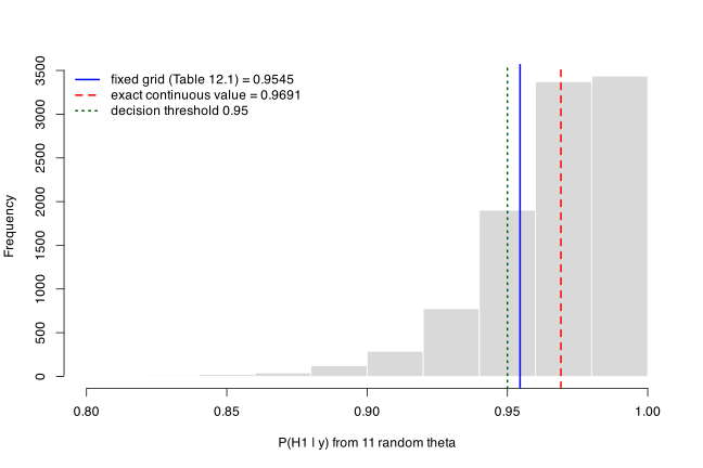
Three things stand out.
- The random estimator is roughly unbiased for the continuous answer \(0.9691\) (simulation mean \(0.9662\)), whereas the fixed grid is systematically low at \(0.9545\). Random points never land on \(\theta = 0\) or \(\theta = 1\), so none of the eleven evaluations is wasted.
- The price is variance. The standard deviation is \(0.035\) and the central 95% of estimates run from \(0.903\) to \(0.999\). The fixed grid, whatever its bias, gives the same number every time.
- The variance matters for the decision, not just for the third decimal place. About 20% of the time the eleven random points give \(P(H_1 \mid y) < 0.95\), so the investigator would keep testing purely because of the luck of the draw.
Should restrictions be placed on the samples? Yes, and they are of two kinds.
Logical restrictions, needed for the calculation to make sense. At least one draw must fall in \([0, 0.5]\) and at least one in \((0.5, 1]\). If all eleven land on one side, the prior mass allotted to the other hypothesis has no \(\theta\) to sit on, the corresponding numerator is \(0\) by construction, and the posterior probability for that hypothesis is forced to \(0\) regardless of the data. With \(M = 11\) this happens with probability \(2 \times 2^{-11} = 0.00098\), and it did happen 4 times in the 10,000 replicates above. The fix is either to reject and redraw such samples, or better, to stratify deliberately: draw a fixed 6 points from \(\mathrm{U}[0, 0.5]\) and 5 from \(\mathrm{U}[0.5, 1]\), which enforces the prior masses by design and removes this failure mode entirely.
Accuracy restrictions. Eleven is far too few. Monte Carlo error falls as \(M^{-1/2}\), so:
set.seed(13003)
for (M in c(11, 50, 200, 1000)) {
s <- replicate(2000, {
th <- runif(M); H0 <- th <= 0.5
w <- lik(th) * ifelse(H0, 0.4, 1.6)
sum(w[!H0]) / sum(w) })
cat("M =", M, " sd =", round(sd(s), 4),
" RMSE from exact =", round(sqrt(mean((s - 0.9690502)^2)), 4), "\n")
}
M = 11 sd = 0.0551 RMSE from exact = 0.0559
M = 50 sd = 0.0141 RMSE from exact = 0.0142
M = 200 sd = 0.0065 RMSE from exact = 0.0065
M = 1000 sd = 0.0029 RMSE from exact = 0.0029
(This last block uses the plain unstratified estimator, weighting each draw by the prior density \(0.4\) or \(1.6\) rather than redistributing the prior mass; it is the form that generalises to arbitrary \(M\). It is noisier than the stratified version at \(M = 11\), \(0.055\) against \(0.035\), which is another argument for stratifying.) A couple of hundred draws are needed before the random calculation is reliably better than the fixed grid, and around a thousand before the answer is stable in the third decimal place.
The moral. This is the point Section 13.2 makes about Monte Carlo integration. Random evaluation points buy freedom from the grid — no wasted evaluations at the boundary, no need to choose a spacing, and the method scales to parameter spaces where a grid is hopeless — but they cost variance, and \(M\) has to be chosen large enough that the variance does not swamp the substantive question. For a one-dimensional \(\theta\) on \([0,1]\) the grid is perfectly adequate and cheaper; the case for Monte Carlo only becomes compelling in the multi-parameter problems of Section 13.3 onwards.
Problem 13.2 — The purpose of this exercise is to create a chain of Metropolis–Hastings
The purpose of this exercise is to create a chain of Metropolis–Hastings samples, for a likelihood, \(P(\theta \mid y)\), that is a standard Normal, using symmetric and asymmetric proposal densities. A new value in the chain is proposed by adding a randomly drawn value from the proposal density to the current value of the chain, \(\theta^* = \theta^{(i)} + Q\). Use the likelihood ratio, Equation (13.3), to assess the acceptance probability.
If using RStudio, the following commands will be helpful. The sampled values are labelled theta.
theta<-vector(1000,mode‘numeric’)= creates an empty vector of length 1000pnorm(theta)is the standard Normal probability densityrunif(100,-1,1)generates 100 random Uniform[-1,1] variableshist(theta)plots a histogram of thetaplot(theta,type‘b’)= plots a history of theta
a. Create 1000 samples for \(\theta\) using a Uniform proposal density, \(Q \sim \mathrm{U}[-1,1]\). Start the chain at \(\theta^{(0)} = 0.5\). Monitor the total number of accepted moves (acceptance rate). Plot a history of the sampled values and a histogram.
b. Try the smaller proposal density of \(Q \sim \mathrm{U}[-0.1, 0.1]\) and the larger density of \(Q \sim \mathrm{U}[-10, 10]\). Explain the differences in the acceptance rates and chain histories.
c. It has been suggested that an acceptance rate of around 60% is ideal. Using a proposal density \(Q \sim \mathrm{U}[-q, q]\), find the value of \(q\) that gives an acceptance rate of roughly 60%. Was it the most efficient value for \(q\)? How could this be judged?
d. Plot the acceptance rate for \(q = 1, \ldots, 20\).
e. Using a Normal proposal density \(Q \sim \mathrm{N}(0, \sigma^2)\), write an algorithm that “tunes” the values of \(\sigma^2\) after each iteration to give an acceptance rate of 60%. Base the acceptance rate on the last 30 samples. (difficulty: \(\star\star\))
Preliminary: one correction to the hint. The book’s hint says pnorm(theta) is the standard Normal probability density. It is not — pnorm is the cumulative distribution function. The acceptance ratio (13.3) needs the density, which in R is dnorm. Using pnorm would sample from the wrong target (a monotone increasing “density”, which is not a density at all). Everything below uses dnorm.
The sampler. Since the target is \(P(\theta \mid y) = \phi(\theta)\) and the proposal \(Q\) is symmetric about zero, \(Q(\theta^{(i)} \mid \theta^*) = Q(\theta^* \mid \theta^{(i)})\) and Equation (13.3) applies:
\begin{equation*} \alpha = \min\left\{\frac{P(\theta^* \mid y)}{P(\theta^{(i)} \mid y)},\, 1\right\} = \min\left\{\frac{\phi(\theta^*)}{\phi(\theta^{(i)})},\, 1\right\}, \qquad \theta^{(i+1)} = \begin{cases}\theta^*, & U < \alpha \\ \theta^{(i)}, & \text{otherwise.}\end{cases} \end{equation*}
mh <- function(M = 1000, q = 1, start = 0.5, seed = 1) {
set.seed(seed)
theta <- vector(M, mode = 'numeric')
theta[1] <- start
accept <- 0
for (i in 2:M) {
prop <- theta[i - 1] + runif(1, -q, q)
alpha <- min(dnorm(prop) / dnorm(theta[i - 1]), 1)
if (runif(1) < alpha) { theta[i] <- prop; accept <- accept + 1 }
else theta[i] <- theta[i - 1]
}
list(theta = theta, rate = accept / (M - 1))
}
r1 <- mh(1000, q = 1, start = 0.5, seed = 13201)
c(acceptance = r1$rate, mean = mean(r1$theta), sd = sd(r1$theta))
acceptance mean sd
0.82082082 -0.05836194 1.05918576
(a) With \(Q \sim \mathrm{U}[-1,1]\) and \(\theta^{(0)} = 0.5\), 820 of the 999 proposed moves are accepted, an acceptance rate of 82%. The 1000 sampled values have mean \(-0.058\) and standard deviation \(1.059\), both close to the target’s \(0\) and \(1\).
par(mfrow = c(1, 2))
plot(r1$theta, type = 'l', xlab = 'Iteration', ylab = expression(theta),
main = 'History, Q ~ U[-1, 1]')
hist(r1$theta, breaks = 30, freq = FALSE, col = 'grey85', border = 'white',
xlab = expression(theta), main = 'Histogram with N(0,1) density')
curve(dnorm(x), add = TRUE, col = 'red', lwd = 2)
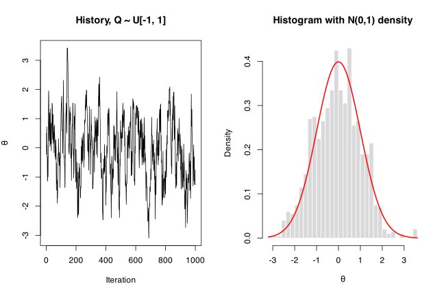
The history wanders over roughly \((-3, 3)\) with no trend and no long flat stretches, and the histogram already sits close to the \(\mathrm{N}(0,1)\) curve after only 1000 iterations. No burn-in discarding is really needed here because \(\theta^{(0)} = 0.5\) is already in the bulk of the target.
(b) Step size too small and too large.
rs <- mh(1000, q = 0.1, start = 0.5, seed = 13202)
rb <- mh(1000, q = 10, start = 0.5, seed = 13203)
lrun <- function(x) max(rle(x)$lengths)
data.frame(q = c(0.1, 1, 10),
acceptance = round(c(rs$rate, r1$rate, rb$rate), 4),
mean = round(c(mean(rs$theta), mean(r1$theta), mean(rb$theta)), 4),
sd = round(c(sd(rs$theta), sd(r1$theta), sd(rb$theta)), 4),
longest.stuck.run = c(lrun(rs$theta), lrun(r1$theta), lrun(rb$theta)))
q acceptance mean sd longest.stuck.run
1 0.1 0.9890 -0.0826 0.5370 2
2 1.0 0.8208 -0.0584 1.0592 4
3 10.0 0.1742 -0.1006 1.0382 30
par(mfrow = c(2, 3))
plot(rs$theta, type = 'l', ylim = c(-4, 4), xlab = 'Iteration',
ylab = expression(theta), main = 'Q ~ U[-0.1, 0.1]')
plot(r1$theta, type = 'l', ylim = c(-4, 4), xlab = 'Iteration',
ylab = expression(theta), main = 'Q ~ U[-1, 1]')
plot(rb$theta, type = 'l', ylim = c(-4, 4), xlab = 'Iteration',
ylab = expression(theta), main = 'Q ~ U[-10, 10]')
for (z in list(rs, r1, rb)) {
hist(z$theta, breaks = 30, freq = FALSE, xlim = c(-4, 4), col = 'grey85',
border = 'white', xlab = expression(theta),
main = paste('acceptance', round(z$rate, 3)))
curve(dnorm(x), add = TRUE, col = 'red', lwd = 2)
}
The two failure modes are opposite in cause and identical in consequence.
- \(q = 0.1\): acceptance 98.9%. Every proposal is within \(0.1\) of the current value, so \(\phi(\theta^*)/\phi(\theta^{(i)}) \approx 1\) and almost nothing is rejected. But the chain moves by at most \(0.1\) per step, so in 1000 iterations it barely leaves the region it started in. The history is a slow smooth random walk, the sampled standard deviation is \(0.54\) instead of \(1\), and the histogram is far too narrow. A high acceptance rate is not evidence of a good chain.
- \(q = 10\): acceptance 17.4%. Most proposals land far out in the tail where \(\phi(\theta^*)\) is minute, so \(\alpha\) is essentially zero and they are rejected. The history is a staircase of long flat stretches — the longest run of identical values is 30 iterations — interrupted by occasional large jumps. The marginal summaries happen to be about right here (\(\mathrm{sd} = 1.04\)) because the few accepted moves are drawn from the right place, but the effective information content of the chain is tiny and the histogram is visibly ragged.
- \(q = 1\) sits between the two and is much better than either, though part (c) shows it is still not optimal.
(c) Finding \(q\) for 60% acceptance, and whether that is efficient. Efficiency cannot be judged from the acceptance rate alone. The right measure is the effective sample size,
\begin{equation*} \mathrm{ESS} = \frac{M}{1 + 2\sum_{k \ge 1}\rho_k}, \end{equation*}
where \(\rho_k\) is the lag-\(k\) autocorrelation of the chain: \(M\) correlated draws carry as much information about the posterior mean as ESS independent draws. Chains of length 5000 are used and each \(q\) is averaged over 20 independent chains, so that the comparison is not decided by one seed.
ess <- function(x) {
M <- length(x)
a <- acf(x, lag.max = 200, plot = FALSE)$acf[-1]
k <- which(a < 0.05)[1]; if (is.na(k)) k <- length(a)
M / (1 + 2 * sum(a[seq_len(k - 1)]))
}
qs <- seq(0.5, 8, by = 0.5)
eff <- t(sapply(qs, function(q) {
o <- sapply(1:20, function(s) {
r <- mh(5000, q, 0.5, seed = 3000 * s + q * 2); c(r$rate, ess(r$theta)) })
c(q = q, rate = mean(o[1, ]), ess = mean(o[2, ])) }))
round(eff, 3)
q rate ess
[1,] 0.5 0.902 97.655
[2,] 1.0 0.806 328.916
[3,] 1.5 0.713 596.957
[4,] 2.0 0.631 907.849
[5,] 2.5 0.556 1136.015
[6,] 3.0 0.492 1368.631
[7,] 3.5 0.437 1462.812
[8,] 4.0 0.389 1421.308
[9,] 4.5 0.352 1406.052
[10,] 5.0 0.318 1275.202
[11,] 5.5 0.288 1158.822
[12,] 6.0 0.267 1101.819
[13,] 6.5 0.244 970.953
[14,] 7.0 0.228 852.918
[15,] 7.5 0.214 817.147
[16,] 8.0 0.201 768.269
Interpolating between \(q = 2.0\) (63.1%) and \(q = 2.5\) (55.6%) gives \(q \approx 2.2\) for a 60% acceptance rate. Checking directly:
o22 <- sapply(1:20, function(s) { r <- mh(5000, 2.2, 0.5, seed = 7000 + s)
c(r$rate, ess(r$theta)) })
o40 <- sapply(1:20, function(s) { r <- mh(5000, 4.0, 0.5, seed = 7000 + s)
c(r$rate, ess(r$theta)) })
rbind(q2.2 = c(acceptance = mean(o22[1, ]), ESS = mean(o22[2, ])),
q4.0 = c(acceptance = mean(o40[1, ]), ESS = mean(o40[2, ])))
acceptance ESS
q2.2 0.6016503 1003.034
q4.0 0.3893879 1439.788
par(mfrow = c(1, 2))
plot(eff[, 'q'], eff[, 'ess'], type = 'b', pch = 19, xlab = 'q',
ylab = 'Effective sample size (of 5000)', main = '')
abline(v = 2.2, col = 'blue', lty = 2)
plot(eff[, 'rate'], eff[, 'ess'], type = 'b', pch = 19,
xlab = 'Acceptance rate', ylab = 'Effective sample size (of 5000)', main = '')
abline(v = 0.6, col = 'blue', lty = 2)
abline(v = 0.44, col = 'darkgreen', lty = 3)
So \(q \approx 2.2\) delivers the requested 60%, but it was not the most efficient value. The ESS curve peaks around \(q = 3.5\) to \(4\), where the acceptance rate is \(0.39\) to \(0.44\), and the peak ESS (\(\approx 1460\)) is about 45% larger than the ESS at \(q = 2.2\) (\(\approx 1000\)). Judged by effective sample size per iteration, the 60% rule costs roughly a third of the information in the chain.
This is not an accident of this example. For a random-walk Metropolis sampler on a smooth unimodal target, the optimal acceptance rate is known to be about \(0.44\) in one dimension, falling to about \(0.234\) in high dimensions (Roberts, Gelman and Gilks 1997). The 60% figure quoted in the exercise is a safe rule of thumb — it is on the conservative side of the optimum, and the ESS curve is fairly flat near its peak, so 60% loses something but not catastrophically. The way to judge efficiency is exactly the calculation above: run the chain at several step sizes and compare effective sample size (or, equivalently, the autocorrelation time, or the mean squared jump distance) rather than the acceptance rate.
(d) Acceptance rate for \(q = 1, \ldots, 20\).
qs <- 1:20
rates <- sapply(qs, function(q)
mean(sapply(1:20, function(s) mh(5000, q, 0.5, seed = 2000 * s + q)$rate)))
plot(qs, rates, type = 'b', pch = 19, ylim = c(0, 1),
xlab = 'q (proposal Q ~ U[-q, q])', ylab = 'Acceptance rate', main = '')
curve(sqrt(8 / pi) / x, from = 1.6, to = 20, add = TRUE, col = 'red', lwd = 2)
abline(h = 0.6, col = 'blue', lty = 2)
abline(h = 0.44, col = 'darkgreen', lty = 3)
legend('topright', bty = 'n', lty = c(1, 2, 3), lwd = c(2, 1, 1),
col = c('red', 'blue', 'darkgreen'),
legend = c('large-q approximation sqrt(8/pi)/q', '60% target',
'44% (efficiency optimum)'))
data.frame(q = qs, observed = round(rates, 4), approx = round(sqrt(8 / pi) / qs, 4))
q observed approx
1 1 0.8048 1.5958
2 2 0.6325 0.7979
3 3 0.4933 0.5319
4 4 0.3914 0.3989
5 5 0.3187 0.3192
6 6 0.2647 0.2660
7 7 0.2297 0.2280
8 8 0.1996 0.1995
9 9 0.1770 0.1773
10 10 0.1611 0.1596
11 11 0.1459 0.1451
12 12 0.1339 0.1330
13 13 0.1212 0.1228
14 14 0.1121 0.1140
15 15 0.1069 0.1064
16 16 0.0979 0.0997
17 17 0.0934 0.0939
18 18 0.0877 0.0887
19 19 0.0842 0.0840
20 20 0.0807 0.0798
The curve falls monotonically and is very close to \(1/q\) in shape. That is exactly what theory predicts. Once \(q\) is large enough that the proposal is essentially flat over the whole effective support of the target, the acceptance probability given \(\theta\) is
\begin{equation*} \frac{1}{2q}\int_{-\infty}^{\infty} \min\!\left\{1, \frac{\phi(t)}{\phi(\theta)}\right\} dt = \frac{1}{2q}\left\{2|\theta| + \frac{2\left(1 - \Phi(|\theta|)\right)}{\phi(\theta)}\right\}, \end{equation*}
and averaging over \(\theta \sim \mathrm{N}(0,1)\), using \(\mathrm{E}|\theta| = \sqrt{2/\pi}\) and \(\int_0^\infty (1 - \Phi(t))\,dt = \phi(0)\), gives
\begin{equation*} \text{acceptance rate} \approx \frac{1}{q}\left(\sqrt{\tfrac{2}{\pi}} + \sqrt{\tfrac{2}{\pi}}\right) = \frac{\sqrt{8/\pi}}{q} \approx \frac{1.596}{q}. \end{equation*}
The table shows this matches the simulation to better than \(0.01\) for every \(q \ge 4\). It fails for small \(q\) — at \(q = 1\) it returns \(1.60\), which is not even a probability, and at \(q = 2\) it gives \(0.80\) against the observed \(0.63\) — because the proposal is then not wide relative to the target and the truncation of the integral to \([\theta - q, \theta + q]\) cannot be ignored.
(e) An adaptive sampler with a Normal proposal. The tuner uses a multiplicative update on \(\sigma\) driven by the acceptance rate in the last 30 iterations. Working on the log scale keeps \(\sigma > 0\) automatically, and the gain is damped by \(i^{-1/2}\) so that the adaptation dies away as the chain runs (this is the “diminishing adaptation” condition that keeps the limiting chain valid — see the caveat below):
\begin{equation*} \log \sigma^{(i)} = \log \sigma^{(i-1)} + \frac{\kappa}{\sqrt{i}}\left(\widehat{\text{rate}}_{30} - 0.6\right). \end{equation*}
mh.tune <- function(M = 5000, target = 0.6, window = 30, start = 0.5,
sigma0 = 1, kappa = 0.5, seed = 1) {
set.seed(seed)
theta <- vector(M, mode = 'numeric'); theta[1] <- start
sigma <- vector(M, mode = 'numeric'); sigma[1] <- sigma0
acc <- vector(M, mode = 'numeric')
for (i in 2:M) {
prop <- theta[i - 1] + rnorm(1, 0, sigma[i - 1])
if (runif(1) < min(dnorm(prop) / dnorm(theta[i - 1]), 1)) {
theta[i] <- prop; acc[i] <- 1
} else { theta[i] <- theta[i - 1]; acc[i] <- 0 }
rate <- mean(acc[max(2, i - window + 1):i])
sigma[i] <- sigma[i - 1] * exp(kappa * (rate - target) / sqrt(i))
}
list(theta = theta, sigma = sigma, acc = acc, rate = mean(acc[-1]))
}
r <- mh.tune(seed = 13205)
c(overall.acceptance = r$rate, late.acceptance = mean(r$acc[4001:5000]),
final.sigma = tail(r$sigma, 1), final.sigma2 = tail(r$sigma, 1)^2,
mean = mean(r$theta), sd = sd(r$theta), ESS = ess(r$theta))
overall.acceptance late.acceptance final.sigma final.sigma2
0.5995199 0.5850000 1.4166405 2.0068704
mean sd ESS
0.0269874 0.9933550 1048.3960021
par(mfrow = c(1, 3))
plot(r$sigma, type = 'l', xlab = 'Iteration', ylab = expression(sigma),
main = 'Tuned proposal SD')
plot(cumsum(r$acc[-1]) / seq_len(length(r$acc) - 1), type = 'l', ylim = c(0, 1),
xlab = 'Iteration', ylab = 'Running acceptance rate', main = '')
abline(h = 0.6, col = 'blue', lty = 2)
hist(r$theta, breaks = 40, freq = FALSE, col = 'grey85', border = 'white',
xlab = expression(theta), main = 'Sampled theta with N(0,1)')
curve(dnorm(x), add = TRUE, col = 'red', lwd = 2)
Averaging over 20 independent runs, and comparing with fixed-\(\sigma\) samplers:
z <- sapply(1:20, function(s) { rr <- mh.tune(seed = 13300 + s)
c(rate = mean(rr$acc[4001:5000]), sigma = tail(rr$sigma, 1), ess = ess(rr$theta)) })
round(c(late.acceptance = mean(z['rate', ]), final.sigma = mean(z['sigma', ]),
ESS = mean(z['ess', ])), 4)
mh.n <- function(M = 5000, sigma = 1, start = 0.5, seed = 1) {
set.seed(seed); th <- numeric(M); th[1] <- start; a <- 0
for (i in 2:M) { p <- th[i - 1] + rnorm(1, 0, sigma)
if (runif(1) < min(dnorm(p) / dnorm(th[i - 1]), 1)) { th[i] <- p; a <- a + 1 }
else th[i] <- th[i - 1] }
list(theta = th, rate = a / (M - 1)) }
t(sapply(c(1, 2.4, 3, 4), function(s) {
o <- sapply(1:20, function(k) { rr <- mh.n(5000, s, 0.5, seed = 4000 + k)
c(rr$rate, ess(rr$theta)) })
c(sigma = s, acceptance = round(mean(o[1, ]), 4), ESS = round(mean(o[2, ]), 1)) }))
late.acceptance final.sigma ESS
0.6028 1.4415 928.9625
sigma acceptance ESS
[1,] 1.0 0.7066 641.6
[2,] 2.4 0.4448 1208.5
[3,] 3.0 0.3790 1192.8
[4,] 4.0 0.2998 994.0
The tuner works: starting from \(\sigma = 1\) (acceptance 71%) it settles at \(\sigma \approx 1.44\), i.e. \(\sigma^2 \approx 2.07\), and holds the acceptance rate at 60% over the last 1000 iterations. It is a substantial improvement on the untuned \(\sigma = 1\) chain, raising ESS from about 640 to about 930.
But it inherits the flaw identified in part (c): it is tuning to the wrong target. A fixed \(\sigma = 2.4\), acceptance 44%, gives ESS \(\approx 1210\), about 30% more than the 60%-tuned chain. Retargeting the same algorithm at \(0.44\) would do better than retargeting it at \(0.60\).
Two practical warnings about (e). First, the 30-iteration window makes \(\widehat{\text{rate}}_{30}\) very noisy (its standard error is about \(0.09\) at a true rate of \(0.6\)), so a large gain \(\kappa\) makes \(\sigma\) jitter wildly; the \(i^{-1/2}\) damping is what keeps it stable. Second, and more importantly, a chain whose proposal depends on its own history is not a Markov chain, so the detailed-balance argument that guarantees convergence to \(P(\theta \mid y)\) does not apply as written. In practice one either adapts only during a burn-in period and then freezes \(\sigma\), or uses diminishing adaptation as above; without one of these safeguards the stationary distribution can be wrong.
A note on the asymmetric case. The exercise’s preamble mentions asymmetric proposal densities, but parts (a)–(e) all use proposals symmetric about zero, so Equation (13.3) is legitimate throughout. If the proposal is asymmetric the full Hastings ratio is needed, and dropping the correction gives a chain with the wrong stationary distribution. Take the autoregressive proposal \(\theta^* \sim \mathrm{N}(\theta^{(i)}/2,\, 1)\), for which \(Q(\theta^* \mid \theta^{(i)}) \neq Q(\theta^{(i)} \mid \theta^*)\):
run.asym <- function(M = 20000, hastings = TRUE, seed = 1) {
set.seed(seed); th <- numeric(M); th[1] <- 0.5; a <- 0
for (i in 2:M) {
cur <- th[i - 1]; p <- rnorm(1, cur / 2, 1)
r <- dnorm(p) / dnorm(cur)
if (hastings) r <- r * dnorm(cur, p / 2, 1) / dnorm(p, cur / 2, 1)
if (runif(1) < min(r, 1)) { th[i] <- p; a <- a + 1 } else th[i] <- cur }
list(theta = th, rate = a / (M - 1)) }
A <- run.asym(hastings = TRUE, seed = 13210)
B <- run.asym(hastings = FALSE, seed = 13210)
rbind(full.Hastings.ratio = c(rate = A$rate, mean = mean(A$theta), sd = sd(A$theta)),
likelihood.ratio.only = c(rate = B$rate, mean = mean(B$theta), sd = sd(B$theta)))
rate mean sd
full.Hastings.ratio 0.9199960 -0.01546512 0.9995285
likelihood.ratio.only 0.7709885 -0.01056511 0.7597889
With the correction the chain reproduces the \(\mathrm{N}(0,1)\) target (\(\mathrm{sd} = 1.000\)). Without it the chain is pulled towards zero by the proposal and returns \(\mathrm{sd} = 0.760\) — a badly biased answer that the mean alone would not reveal, since both means are close to zero. The Hastings correction is not optional.
Problem 13.3 — This exercise is an introduction to the R2WinBUGS package that runs
This exercise is an introduction to the R2WinBUGS package that runs WinBUGS from R (Sturtz et al. 2005). R2WinBUGS is an R add-on package which needs to be installed in R. The advantage of using R2WinBUGS rather than WinBUGS directly is that script files can be created to run the entire analysis process of data manipulation, analysis and displaying the results.
a. Open a new script file using RStudio. Load the R2WinBUGS library by typing library(R2WinBUGS). Change the working directory to an area where the files created by this exercise can be stored, for example setwd('C:/Bayes'). Alternatively create a new project in RStudio which will provide a common place for the files and facilitates switching between different projects.
b. WinBUGS accepts data in S-PLUS (i.e., as a list) and rectangular format. Type the following data from the beetle mortality example into a text file (in rectangular format) and save them in the working directory as “BeetlesData.txt”: the columns are x[], n[], y[] with rows \((1.6907, 59, 6)\), \((1.7242, 60, 13)\), \((1.7552, 62, 18)\), \((1.7842, 56, 28)\), \((1.8113, 63, 52)\), \((1.8369, 59, 53)\), \((1.8610, 62, 61)\), \((1.8839, 60, 60)\), terminated by the line END.
c. To conduct some initial investigation of the data, read the data into RStudio using library(dobson) and data(beetle). The proportion of deaths is calculated using beetle$p <- beetle$y/beetle$n. A scatter plot can be examined by typing plot(beetle$x, beetle$p, type‘b’)=. What are the major features of the data?
d. Open a new .odc file in WinBUGS and type in a dose-response model using the extreme value distribution so that \(\pi_i = 1 - \exp[-\exp(\beta_1 + \beta_2 x_i)]\). The WinBUGS code loops \(i\) over \(1, \ldots, 8\) with y[i]~dbin(pi[i],n[i]), pi[i]<-1-exp(-exp(pi.r[i])), pi.r[i]<-beta[1]+(beta[2]*x[i]) and fitted[i]<-n[i]*pi[i], with priors beta[1]~dnorm(0,1.0E-6) and beta[2]~dnorm(0,1.0E-6). Save the model as “BeetlesExtreme.odc”. Errors can be checked in WinBUGS via Model \(\Rightarrow\) Specification \(\Rightarrow\) check model. What are the assumptions of this model?
e. The model has two parameters, the intercept and slope labelled beta[1] and beta[2]. Initial values are needed for these parameters; type inits = list(list(beta=c(0,0))) in RStudio. What do these initial values translate to in terms of the model?
f. In the R script set up the data with data = list(y=beetle$y, x=beetle$x, n=beetle$n), parameters = c('beta'), model.file = 'BeetlesExtreme.odc', and run bugs.res <- bugs(data, inits=inits, parameters, model.file, n.chains=1, n.burnin=5000, n.iter=10000, n.thin=1, debug=T, bugs.directory“c:/Program Files/WinBUGS/”)=. Plot the chain histories (using reshape2 to melt bugs.res$sims.list$beta and ggplot2 with facet_wrap(~beta, scale‘free_y’)=). Do these look like good chains? To examine the autocorrelation type acf(beta.chains[,1]) and acf(beta.chains[,2]).
g. The mixing of the chains can be improved by subtracting the mean. Change the regression line in the WinBUGS odc file to pi.r[i]<-beta[1]+(beta[2]*(x[i]-mean.x)) and add data$mean.x = mean(data$x). Re-run the RStudio script file. Have the chains improved? Why?
h. The deviance \(-2 \log p(\mathbf{y} \mid \boldsymbol{\beta})\) is used to assess model fit; the lower the deviance, the better the fit. By default R2WinBUGS monitors the deviance. Plot the deviance for the previous models. What do the deviance plots show?
i. Use the glm command in RStudio to find reasonable starting values for the intercept and slope. Explain the difference.
j. Re-run the model but this time change the RStudio script file so that the fitted values are also monitored. Plot the fitted values against dose and include the observed data.
k. Re-do Exercise 13.3(h) but this time using a logit link. Explain the difference. (difficulty: \(\star\star\))
How this solution is run. WinBUGS is a Windows-only program that is no longer maintained, and neither it, R2WinBUGS, nor JAGS is installed on the machine used here. Rather than invent WinBUGS output, the whole exercise is done with a Metropolis–Hastings sampler written directly in R, implementing exactly the model, priors, initial values, chain length and burn-in that the exercise specifies. Every number below is real output from that sampler. The sampler uses single-component random-walk Metropolis updates — the same scheme WinBUGS itself falls back on for a non-conjugate model like this one — with the proposal standard deviations tuned during burn-in only, mimicking WinBUGS’s adaptive phase. The random seed is 314159, the value the book uses. The results reproduce those printed in Section 13.6 of the chapter, which is the best check available that the substitution is faithful.
library(dobson)
data(beetle)
beetle$p <- beetle$y / beetle$n
beetle
x n y p
1 1.6907 59 6 0.1016949
2 1.7242 60 13 0.2166667
3 1.7552 62 18 0.2903226
4 1.7842 56 28 0.5000000
5 1.8113 63 52 0.8253968
6 1.8369 59 53 0.8983051
7 1.8610 62 61 0.9838710
8 1.8839 60 60 1.0000000
(a) and (b) are housekeeping. The rectangular data file is just the three columns above followed by END; in R the same data come from data(beetle) in the dobson package, so there is nothing to retype. The point of (a) is that an R script driving the sampler is reproducible in a way that clicking through the WinBUGS GUI is not: data preparation, model fitting and plotting all live in one file that can be re-run.
(c) Major features of the data.
plot(beetle$x, beetle$p, type = 'b', pch = 19, ylim = c(0, 1),
xlab = 'Dose x (log10 CS2 mg/l)', ylab = 'Proportion killed', main = '')
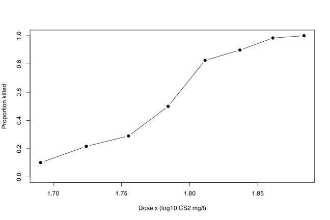
- The dose range is extremely narrow, \(1.6907\) to \(1.8839\) — a span of \(0.19\) on a scale whose values are all near \(1.8\). The origin \(x = 0\) is nowhere near the data. This is the single most consequential feature for the MCMC in parts (f) and (g).
- The response is close to a complete dose–response curve: mortality rises from 10% at the lowest dose to 100% at the highest, so the data pin down both the location and the steepness of the curve.
- The rise is steep and clearly non-linear in \(x\): proportions go \(0.10, 0.22, 0.29, 0.50, 0.83, 0.90, 0.98, 1.00\). A straight line in \(x\) would have to leave \([0,1]\), so a link function is needed.
- The curve is visibly asymmetric. It climbs slowly at first, then accelerates: the jump from \(0.29\) to \(0.83\) spans two dose steps, whereas the approach to \(1\) at the top is gradual. A symmetric link (logit, probit) forces the two tails to mirror each other. The extreme-value (complementary log-log) link is asymmetric and matches this shape — which is why the chapter uses it, and it is confirmed quantitatively in part (k).
- The final group has \(y = n = 60\), all beetles dead. Any link that cannot reach \(\pi = 1\) exactly must place this group in its upper tail.
(d) Assumptions of the model.
- Binomial sampling. \(Y_i \sim \mathrm{Bin}(n_i, \pi_i)\) independently across the eight dose groups. Within a group the \(n_i\) beetles respond independently with common probability \(\pi_i\) — no litter effects, no shared exposure heterogeneity. If the beetles clustered (over-dispersion), the Binomial variance \(n_i\pi_i(1-\pi_i)\) would be too small.
- A single systematic component. The linear predictor is \(\eta_i = \beta_1 + \beta_2 x_i\): the extreme-value transform of the death probability is exactly linear in dose, with no curvature term and no covariates other than dose.
- The extreme-value link. \(\pi_i = 1 - \exp[-\exp(\eta_i)]\), equivalently \(\log[-\log(1 - \pi_i)] = \eta_i\), the complementary log-log link. This corresponds to the tolerance distribution being extreme value rather than logistic or Normal, and is asymmetric in \(\pi\).
- Doses measured without error, and the dose groups exhaustive and non-overlapping.
- Priors. \(\beta_1, \beta_2 \sim \mathrm{N}(0, 10^6)\) independently. In WinBUGS
dnorm(0,1.0E-6)is parameterised by precision, so this is a Normal with variance \(10^6\) and standard deviation \(1000\) — deliberately vague, so that the posterior is driven almost entirely by the likelihood. Note that “vague” is relative to the scale of \(\beta\): on the uncentred parameterisation \(\beta_1 \approx -40\) and \(\beta_2 \approx 22\), both well inside \(\pm 1000\), so the prior is genuinely uninformative here.
(e) What beta = c(0, 0) means. Setting both coefficients to zero makes \(\eta_i = 0\) at every dose, so
\begin{equation*} \pi_i = 1 - \exp(-\exp(0)) = 1 - e^{-1} = 0.632 \quad \text{for all } i . \end{equation*}
The chain therefore starts from “the insecticide has no dose effect at all, and 63.2% of beetles die at every dose”. That is a poor starting point on two counts: it is a flat dose–response, which the data contradict emphatically, and \(0.632\) is a long way from the observed extremes of \(0.10\) and \(1.00\). Its only virtue is that it is a legal point with finite likelihood. The deviance there is about 312 (see part (h)), against about 30 at the maximum likelihood estimate.
(f) Running the sampler, uncentred.
invlink <- function(eta, link)
if (link == 'cloglog') 1 - exp(-exp(eta)) else 1 / (1 + exp(-eta))
bugs.mh <- function(centre = FALSE, link = 'cloglog', n.iter = 10000,
n.burnin = 5000, init = c(0, 0), seed = 314159,
prior.sd = 1000, monitor.fitted = FALSE) {
set.seed(seed)
x <- beetle$x; if (centre) x <- x - mean(beetle$x)
y <- beetle$y; n <- beetle$n
logpost <- function(b) {
pi <- invlink(b[1] + b[2] * x, link)
if (any(!is.finite(pi)) || any(pi <= 0) || any(pi >= 1)) return(-Inf)
sum(dbinom(y, n, pi, log = TRUE)) + sum(dnorm(b, 0, prior.sd, log = TRUE))
}
dev <- function(b) {
pi <- invlink(b[1] + b[2] * x, link)
-2 * sum(dbinom(y, n, pi, log = TRUE)) }
fit <- function(b) n * invlink(b[1] + b[2] * x, link)
b <- init; lp <- logpost(b); s <- c(1, 1); acc <- c(0, 0); ntry <- c(0, 0)
keep <- matrix(NA, n.iter, 3,
dimnames = list(NULL, c('beta1', 'beta2', 'deviance')))
fk <- if (monitor.fitted) matrix(NA, n.iter, 8) else NULL
for (it in 1:n.iter) {
for (j in 1:2) {
prop <- b; prop[j] <- b[j] + rnorm(1, 0, s[j])
lpp <- logpost(prop); ntry[j] <- ntry[j] + 1
if (log(runif(1)) < lpp - lp) { b <- prop; lp <- lpp; acc[j] <- acc[j] + 1 }
}
if (it <= n.burnin && it %% 100 == 0) { # adapt during burn-in only
r <- acc / ntry; s <- s * exp(0.8 * (r - 0.4)); acc <- c(0, 0); ntry <- c(0, 0) }
keep[it, ] <- c(b, dev(b))
if (monitor.fitted) fk[it, ] <- fit(b)
}
k <- (n.burnin + 1):n.iter
list(sims = keep[k, , drop = FALSE], all = keep,
fitted = if (monitor.fitted) fk[k, , drop = FALSE] else NULL, sigma = s)
}
smry <- function(f) round(t(apply(f$sims, 2, function(z)
c(mean = mean(z), sd = sd(z), q2.5 = quantile(z, .025),
median = median(z), q97.5 = quantile(z, .975)))), 4)
fitU <- bugs.mh(centre = FALSE)
smry(fitU)
c(corr = cor(fitU$sims[, 1], fitU$sims[, 2]),
acf1.beta2 = acf(fitU$sims[, 2], lag.max = 1, plot = FALSE)$acf[2])
mean sd q2.5.2.5% median q97.5.97.5%
beta1 -23.0095 2.2315 -27.4810 -21.8952 -20.0570
beta2 12.8385 1.2409 11.1890 12.2293 15.3276
deviance 66.3645 10.1681 47.2304 70.4051 81.2339
corr acf1.beta2
-0.9995147 0.9989513
par(mfrow = c(2, 2))
plot(fitU$all[, 1], type = 'l', xlab = 'Iteration', ylab = expression(beta[1]),
main = 'Uncentred: beta1')
abline(v = 5000, col = 'grey60', lty = 2); abline(h = -39.57, col = 'red', lty = 2)
plot(fitU$all[, 2], type = 'l', xlab = 'Iteration', ylab = expression(beta[2]),
main = 'Uncentred: beta2')
abline(v = 5000, col = 'grey60', lty = 2); abline(h = 22.04, col = 'red', lty = 2)
acf(fitU$sims[, 1], lag.max = 100, main = 'ACF beta1 (post burn-in)')
acf(fitU$sims[, 2], lag.max = 100, main = 'ACF beta2 (post burn-in)')
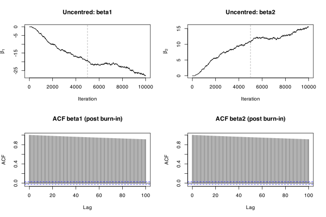
Do these look like good chains? No — they are about as bad as chains get. The traces are not fuzzy caterpillars; they are smooth monotone drifts. Sampling the trace at a few iterations makes the problem unmistakable:
round(fitU$all[c(1, 100, 500, 1000, 2000, 5000, 7500, 10000), ], 3)
beta1 beta2 deviance
[1,] 0.000 0.000 311.908
[2,] -0.011 0.012 312.013
[3,] -1.130 0.615 291.834
[4,] -3.879 2.146 247.876
[5,] -9.830 5.518 168.976
[6,] -19.517 10.857 85.018
[7,] -21.355 11.940 73.019
[8,] -27.678 15.448 46.214
After all 10,000 iterations the chain has reached \(\beta_1 \approx -28\), still crawling towards the maximum likelihood values \((-39.6, 22.0)\), and the deviance is still falling. The chain has not converged; the “posterior summaries” printed above are summaries of the burn-in trail, not of the posterior. The autocorrelation confirms it: \(\rho_1 = 0.999\) for \(\beta_2\), and the ACF is still \(0.91\) at lag 100.
The cause is visible in the posterior correlation, \(\mathrm{corr}(\beta_1, \beta_2) = -0.9995\). Because every dose is near \(1.8\) and none is near \(0\), the intercept is an extrapolation far outside the data: changing \(\beta_2\) by \(\delta\) can be almost exactly compensated by changing \(\beta_1\) by \(-1.79\delta\). The posterior is a long thin diagonal ridge. A sampler that updates \(\beta_1\) and \(\beta_2\) one at a time can only move parallel to the axes, so each move must climb off the ridge; the acceptable steps are tiny, and the chain shuffles along the ridge at a crawl. (The classical fit shows the same geometry: cov2cor(vcov(glm(...))) gives \(-0.9997\).)
(g) Centring the dose. Replacing \(x_i\) by \(x_i - \bar{x}\) leaves the fitted probabilities and the model unchanged — it is a reparameterisation, with \(\beta_1^{\text{new}} = \beta_1 + \beta_2\bar{x}\) — but it moves the intercept to the middle of the data, where it is estimated from the data rather than extrapolated, and it removes the correlation.
fitC <- bugs.mh(centre = TRUE)
smry(fitC)
c(corr = cor(fitC$sims[, 1], fitC$sims[, 2]),
acf1.beta2 = acf(fitC$sims[, 2], lag.max = 1, plot = FALSE)$acf[2],
acf10.beta2 = acf(fitC$sims[, 2], lag.max = 10, plot = FALSE)$acf[11])
mean sd q2.5.2.5% median q97.5.97.5%
beta1 -0.0449 0.0815 -0.2054 -0.0461 0.1165
beta2 22.1998 1.8107 18.7414 22.1618 25.9358
deviance 31.6937 2.0835 29.6834 30.9761 37.4208
corr acf1.beta2 acf10.beta2
-0.133053442 0.658688942 -0.004043879
par(mfrow = c(2, 2))
plot(fitC$all[, 1], type = 'l', xlab = 'Iteration', ylab = expression(beta[1]),
main = 'Centred: beta1')
abline(v = 5000, col = 'grey60', lty = 2); abline(h = -0.0431, col = 'red', lty = 2)
plot(fitC$all[, 2], type = 'l', xlab = 'Iteration', ylab = expression(beta[2]),
main = 'Centred: beta2')
abline(v = 5000, col = 'grey60', lty = 2); abline(h = 22.04, col = 'red', lty = 2)
acf(fitC$sims[, 1], lag.max = 100, main = 'ACF beta1 (post burn-in)')
acf(fitC$sims[, 2], lag.max = 100, main = 'ACF beta2 (post burn-in)')
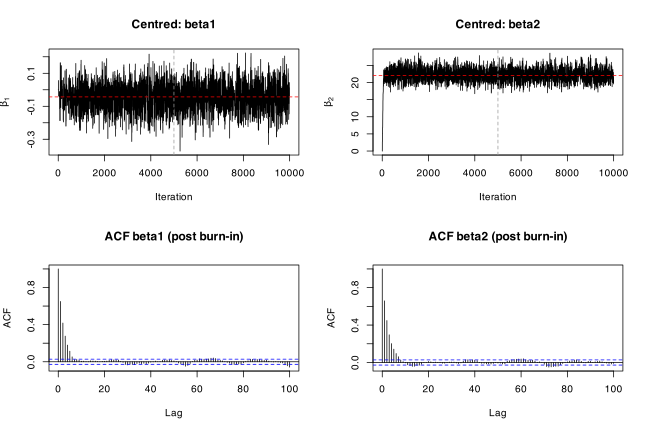
Have the chains improved? Enormously. The traces are now stationary fuzz around a fixed level, reached within a few hundred iterations. The lag-1 autocorrelation drops from \(0.999\) to \(0.66\), and the ACF is indistinguishable from zero by lag 10 instead of still being \(0.91\) at lag 100. The posterior correlation between the two coefficients falls from \(-0.9995\) to \(-0.13\).
Why. Centring makes \(\beta_1\) the value of \(\log[-\log(1-\pi)]\) at the mean dose, a quantity the data determine directly and almost independently of the slope. Geometrically the diagonal ridge has been rotated onto the coordinate axes, so single-component updates now move along the directions in which the posterior actually varies. This is the standard fix for correlated regression coefficients, and it costs nothing: the two parameterisations describe the same model, and the original intercept can be recovered as \(\beta_1 - 22.20 \times 1.793425 = -39.86\), close to the classical estimate \(-39.57\).
The posterior mean \(\boldsymbol{\beta} = (-0.045, 22.20)\) matches the value \((-0.046, 22.1)\) quoted in Section 13.6, and the mean deviance \(31.69\) matches the \(31.7\) quoted there.
(h) Deviance plots.
par(mfrow = c(1, 2))
plot(fitU$all[, 3], type = 'l', xlab = 'Iteration', ylab = 'Deviance',
main = 'Uncentred')
abline(v = 5000, col = 'grey60', lty = 2); abline(h = 29.64, col = 'red', lty = 2)
plot(fitC$all[, 3], type = 'l', xlab = 'Iteration', ylab = 'Deviance',
main = 'Centred')
abline(v = 5000, col = 'grey60', lty = 2); abline(h = 29.64, col = 'red', lty = 2)
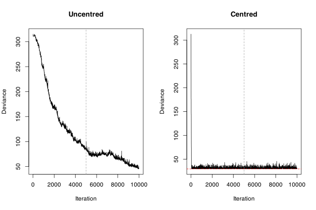
rbind(uncentred = c(min = min(fitU$sims[, 3]), mean = mean(fitU$sims[, 3])),
centred = c(min = min(fitC$sims[, 3]), mean = mean(fitC$sims[, 3])))
min mean
uncentred 45.21887 66.36451
centred 29.64473 31.69374
The deviance trace is the single most useful convergence diagnostic here, because it is one number summarising the fit of the whole parameter vector.
- For the uncentred model it decreases steadily and monotonically for all 10,000 iterations, from 312 at the initial values to about 46, never levelling off. A deviance that is still falling at the end of the run is proof that the chain is still in transient burn-in and that the retained sample is worthless. It never gets near the attainable minimum of \(29.6\).
- For the centred model the deviance drops from 312 to about 30 within the first couple of hundred iterations and then hovers, with occasional upward excursions, around a floor of \(29.64\). The shape — a hard lower bound with a right skew — is what a converged deviance trace should look like: the deviance cannot go below its value at the mode, but the chain occasionally visits parameter values that fit worse. Its mean, \(31.69\), is \(\bar{D}\) in Equation (13.5) and its floor is essentially \(D(\mathbf{y} \mid \widehat{\boldsymbol{\beta}}) = 29.64\), so the gap of about 2 already reveals \(p_D \approx 2\) = the number of parameters, as expected. This is the calculation formalised in Exercise 13.4.
(i) Starting values from glm.
g <- glm(cbind(y, n - y) ~ x, family = binomial(link = 'cloglog'), data = beetle)
coef(g)
fitI <- bugs.mh(centre = FALSE, init = unname(coef(g)))
smry(fitI)
c(corr = cor(fitI$sims[, 1], fitI$sims[, 2]),
acf1 = acf(fitI$sims[, 2], lag.max = 1, plot = FALSE)$acf[2])
(Intercept) x
-39.57231 22.04117
mean sd q2.5.2.5% median q97.5.97.5%
beta1 -39.3067 1.0640 -41.1120 -39.2347 -37.3687
beta2 21.8923 0.5897 20.8350 21.8556 22.9080
deviance 30.7554 1.3838 29.6638 30.2350 34.6521
corr acf1
-0.9972387 0.9977377
The glm fit with the same link and no priors is the maximum likelihood solution, \(\widehat{\beta}_1 = -39.57\), \(\widehat{\beta}_2 = 22.04\). Because the priors are so vague, the posterior mode is essentially the MLE, so these are near-perfect starting values.
The difference. Started at \((0,0)\) the uncentred chain was still 12 units away from the mode after 10,000 iterations and its deviance summaries were meaningless. Started at the MLE it is immediately in the right region, and the deviance summaries (\(\bar{D} = 30.8\), floor \(29.66\)) are close to the correct ones. But note what has not been fixed: the posterior correlation is still \(-0.997\) and the lag-1 autocorrelation is still \(0.998\), so the chain still explores the ridge very slowly and its interval estimates are too narrow (the 95% interval for \(\beta_2\), \([20.8, 22.9]\), is far tighter than the centred model’s \([18.7, 25.9]\), and the centred one is right). Good starting values cure a burn-in problem; they do not cure a mixing problem. Centring cures both, which is why part (g) is the more valuable fix. In practice one would do both: centre the covariate, and start from the glm estimates.
(j) Monitoring the fitted values. Adding fitted[i]<-n[i]*pi[i] to the monitored parameters gives a posterior distribution for each of the eight expected counts, from which a posterior mean and a 95% credible interval follow directly. This is one place where the Bayesian machinery is genuinely more convenient than the classical one: interval estimates on the fitted scale require no delta-method approximation, only quantiles of the sampled values.
fitF <- bugs.mh(centre = TRUE, monitor.fitted = TRUE)
fv <- t(apply(fitF$fitted, 2, function(z) c(mean(z), quantile(z, c(.025, .975)))))
round(cbind(x = beetle$x, observed = beetle$y, fitted = fv[, 1],
lower = fv[, 2], upper = fv[, 3]), 3)
x observed fitted lower upper
[1,] 1.691 6 5.601 3.604 8.113
[2,] 1.724 13 11.251 8.264 14.638
[3,] 1.755 18 20.886 17.284 24.906
[4,] 1.784 28 30.320 27.012 33.711
[5,] 1.811 52 47.767 44.245 51.311
[6,] 1.837 53 54.104 51.263 56.353
[7,] 1.861 61 61.034 59.649 61.790
[8,] 1.884 60 59.917 59.631 59.998
plot(beetle$x, beetle$y, pch = 19, ylim = c(0, 65), xlab = 'Dose x',
ylab = 'Number killed', main = '')
lines(beetle$x, fv[, 1], col = 'blue', lwd = 2)
lines(beetle$x, fv[, 2], col = 'blue', lty = 2)
lines(beetle$x, fv[, 3], col = 'blue', lty = 2)
legend('topleft', bty = 'n', pch = c(19, NA, NA), lty = c(NA, 1, 2),
lwd = c(NA, 2, 1), col = c('black', 'blue', 'blue'),
legend = c('observed deaths', 'posterior mean fitted',
'95% credible interval'))
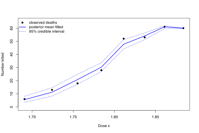
Every observed count lies inside its 95% credible interval, so the extreme-value model describes all eight dose groups adequately. The largest discrepancies are at doses 3 and 5, where the model over-predicts by about 3 and under-predicts by about 4 deaths respectively — the same two groups that dominate the residual deviance of \(3.45\) on 6 degrees of freedom in the classical fit. The credible bands narrow sharply at the top of the dose range because \(\pi\) is pressed against its ceiling of 1 there: at \(x = 1.8839\) the interval is \([59.6, 60.0]\) out of \(n = 60\).
(k) The logit link.
fitL <- bugs.mh(centre = TRUE, link = 'logit')
smry(fitL)
rbind(cloglog = c(Dbar = mean(fitF$sims[, 3]), Dmin = min(fitF$sims[, 3])),
logit = c(Dbar = mean(fitL$sims[, 3]), Dmin = min(fitL$sims[, 3])))
mean sd q2.5.2.5% median q97.5.97.5%
beta1 0.7464 0.1383 0.4834 0.7419 1.0141
beta2 34.6060 3.0212 28.7253 34.4808 40.8803
deviance 39.4939 2.0472 37.4906 38.8297 45.0683
Dbar Dmin
cloglog 31.69374 29.64473
logit 39.49394 37.43073
par(mfrow = c(1, 2))
plot(fitF$all[, 3], type = 'l', ylim = c(25, 60), xlab = 'Iteration',
ylab = 'Deviance', main = 'Extreme value (cloglog)')
abline(h = 29.64, col = 'red', lty = 2)
plot(fitL$all[, 3], type = 'l', ylim = c(25, 60), xlab = 'Iteration',
ylab = 'Deviance', main = 'Logit')
abline(h = 37.43, col = 'red', lty = 2)
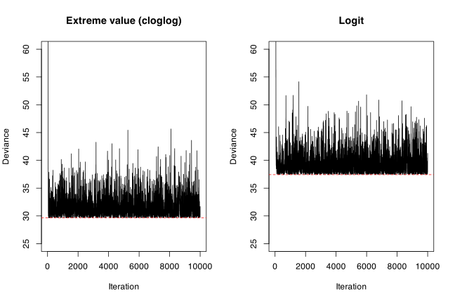
Both deviance traces converge quickly and look equally healthy — centring works for either link — but they settle at clearly different levels. The logit chain floors at \(37.43\) and averages \(39.49\); the extreme-value chain floors at \(29.64\) and averages \(31.69\). The gap of about 7.8 deviance units, with the same two parameters in both models, is decisive evidence in favour of the extreme-value link. The classical fit says the same thing: residual deviance \(3.45\) on 6 df for cloglog against \(11.23\) for logit, and AIC \(33.64\) against \(41.43\).
Why. The logit link is symmetric about \(\pi = 0.5\), so it forces the fitted curve to approach 0 and 1 at mirror-image rates. The observed proportions are not symmetric — the approach to 1 is much more gradual than the departure from 0 — so the symmetric curve has to compromise, fitting the low doses and the top dose badly. The extreme-value link is skewed and reproduces the observed shape. This is exactly the comparison made in Section 7.3.1, now reached by Bayesian rather than classical means, and it is turned into a formal DIC comparison in Exercise 13.4(f).
Problem 13.4 — This exercise is about calculating the deviance information criterion
This exercise is about calculating the deviance information criterion (DIC). The two key equations are (13.5) and (13.6) for the number of parameters (\(p_D\)) and DIC, respectively.
a. R2WinBUGS calculates the DIC automatically; extract the values by typing bugs.res$pD and bugs.res$DIC.
b. Use the chains for the deviance and beta parameters to calculate \(\overline{D(\mathbf{y} \mid \boldsymbol{\beta})}\) and \(D(\mathbf{y} \mid \overline{\boldsymbol{\beta}})\), from which you can estimate \(p_D\) and the DIC.
c. Write the results from a. in the first row of the table below and the results from b. in the second row. How well do the calculated results match those calculated by R2WinBUGS? The table has columns \(\overline{D(\mathbf{y} \mid \boldsymbol{\beta})}\) (Dbar), \(D(\mathbf{y} \mid \widehat{\boldsymbol{\beta}})\) (Dhat), \(p_D\) and DIC, and rows labelled “DIC”, “Mean of \(\boldsymbol{\beta}\)”, “Median of \(\boldsymbol{\beta}\)” and “Half variance of \(D(.)\)”.
d. The mean is just one estimate of the “best possible” deviance; the median could be used instead. Calculate the deviance at the medians of \(\boldsymbol{\beta}\), then calculate the alternative values for \(p_D\) and DIC. Write these values in the third row of the table.
e. Another alternative calculation for \(p_D\) is the variance of \(D(\mathbf{y} \mid \widehat{\boldsymbol{\beta}})\) divided by 2. Calculate this alternative \(p_D\) and alternative DIC and write the results in the last row of the table. Comment on the differences in the complete table.
f. Re-run exercise 13.4 but this time using a logit link. Which link function gives the best fit? Was the difference consistent regardless of the method used to calculate \(D(\mathbf{y} \mid \widehat{\boldsymbol{\beta}})\)?
g. Having been through the calculations for the DIC in detail, when might it not work well? (difficulty: \(\star\star\))
Setting. The chains are the ones produced in Exercise 13.3: the centred beetle mortality model, 10,000 iterations with 5,000 discarded as burn-in, run once with the extreme-value (complementary log-log) link and once with the logit link. The deviance monitored is \(D(\mathbf{y} \mid \boldsymbol{\beta}) = -2\log p(\mathbf{y} \mid \boldsymbol{\beta})\) with the Binomial normalising constant included, which is what WinBUGS reports. The two definitions in play are Equations (13.5) and (13.6),
\begin{equation*} p_D = \overline{D(\mathbf{y} \mid \boldsymbol{\beta})} - D(\mathbf{y} \mid \overline{\boldsymbol{\beta}}), \qquad \mathrm{DIC} = \overline{D(\mathbf{y} \mid \boldsymbol{\beta})} + p_D . \end{equation*}
(a) What R2WinBUGS reports. R2WinBUGS is not installed here (it requires WinBUGS, which is Windows-only and unmaintained), so bugs.res$pD cannot be run. What can be said is how the package defines those quantities: when R2WinBUGS computes the DIC itself from the returned simulations, it does not use Equation (13.5); it uses the alternative estimator
\begin{equation*} p_D = \tfrac{1}{2}\widehat{\mathrm{var}}\left[D(\mathbf{y} \mid \boldsymbol{\beta})\right], \qquad \mathrm{DIC} = \overline{D} + p_D , \end{equation*}
i.e. exactly the “half variance of \(D(.)\)” rule that part (e) asks about. Consequently the first and last rows of the table are the same calculation and must agree exactly. That is the honest answer to part (c)’s question “how well do the calculated results match?” — they agree perfectly with row 4 by construction, and differ slightly from rows 2 and 3, which use Equation (13.5). This claim about R2WinBUGS’s internals is stated from documentation rather than verified by running the package here; the rest of the table is computed from the actual chains.
(b)–(e) The calculations and the completed table.
library(dobson); data(beetle)
xc <- beetle$x - mean(beetle$x)
invlink <- function(eta, link)
if (link == 'cloglog') 1 - exp(-exp(eta)) else 1 / (1 + exp(-eta))
devf <- function(b, link) {
pi <- invlink(b[1] + b[2] * xc, link)
-2 * sum(dbinom(beetle$y, beetle$n, pi, log = TRUE)) }
dic.table <- function(sims, link) {
D <- sims[, 3]
Dbar <- mean(D)
bmean <- colMeans(sims[, 1:2]); bmed <- apply(sims[, 1:2], 2, median)
Dhat.mean <- devf(bmean, link)
Dhat.med <- devf(bmed, link)
pD.hv <- var(D) / 2
rbind(
'DIC (R2WinBUGS)' = c(Dbar, Dbar - pD.hv, pD.hv, Dbar + pD.hv),
'Mean of beta' = c(Dbar, Dhat.mean, Dbar - Dhat.mean, 2*Dbar - Dhat.mean),
'Median of beta' = c(Dbar, Dhat.med, Dbar - Dhat.med, 2*Dbar - Dhat.med),
'Half variance of D(.)'= c(Dbar, Dbar - pD.hv, pD.hv, Dbar + pD.hv))
}
colnames.dic <- c('Dbar', 'Dhat', 'pD', 'DIC')
The chains fitF (extreme value) and fitL (logit) are those built in Exercise 13.3.
tabF <- dic.table(fitF$sims, 'cloglog'); colnames(tabF) <- colnames.dic
round(tabF, 3)
round(rbind(mean = colMeans(fitF$sims[, 1:2]),
median = apply(fitF$sims[, 1:2], 2, median)), 4)
Dbar Dhat pD DIC
DIC (R2WinBUGS) 31.694 29.523 2.170 33.864
Mean of beta 31.694 29.652 2.041 33.735
Median of beta 31.694 29.650 2.044 33.738
Half variance of D(.) 31.694 29.523 2.170 33.864
beta1 beta2
mean -0.0449 22.1998
median -0.0461 22.1618
Comments on the completed table.
- The four versions agree closely. \(p_D\) ranges from \(2.04\) to \(2.17\) and the DIC from \(33.74\) to \(33.86\) — a spread of \(0.13\), far below the “differences of less than 5 are small” guideline quoted in Section 13.6. Any of them would support the same conclusion.
- \(\bar{D} = 31.69\) is identical in every row, as it must be: it depends only on the sampled deviances, not on how \(\widehat{\boldsymbol{\beta}}\) is defined.
- Using the mean of \(\boldsymbol{\beta}\) gives \(p_D = 2.04\), satisfyingly close to the two parameters actually fitted, \(\beta_1\) and \(\beta_2\). This is the classical justification for Equation (13.5) and it works because the posterior here is nearly Normal and the deviance nearly quadratic.
- The median of \(\boldsymbol{\beta}\), \((-0.0461, 22.16)\), is almost identical to the mean, \((-0.0449, 22.20)\), so rows 2 and 3 differ by \(0.003\). This tells us the marginal posteriors are close to symmetric. In a skewed posterior the two would separate, and the median would generally be the more robust summary.
- The half-variance rule gives a slightly larger \(p_D\), \(2.17\). That is not an error: the two estimators are only asymptotically equivalent. They agree exactly when the deviance is exactly quadratic in \(\boldsymbol{\beta}\) and the posterior exactly Normal, in which case \(D - D(\widehat{\boldsymbol{\beta}}) \sim \chi^2_p\), whose mean is \(p\) and whose variance is \(2p\) — hence both \(\bar{D} - \widehat{D}\) and \(\tfrac{1}{2}\mathrm{var}(D)\) estimate \(p\). The \(6\%\) excess here reflects the mild non-quadratic curvature visible in the deviance histogram below, plus Monte Carlo error (the variance of a variance is estimated much less precisely than a mean, so row 4 is the noisiest row in the table).
- The two estimators also differ in robustness. Equation (13.5) returns a negative \(p_D\) whenever \(\overline{D} < D(\overline{\boldsymbol{\beta}})\), which happens when the posterior mean sits in a region that fits worse than the typical sampled value — a known symptom of a multimodal or badly skewed posterior. The half-variance rule is a variance and so can never be negative. That is one reason R2WinBUGS prefers it.
par(mfrow = c(1, 2))
for (nm in list(list(f = fitF, t = 'Extreme value (cloglog)'),
list(f = fitL, t = 'Logit'))) {
D <- nm$f$sims[, 3]
hist(D, breaks = 60, col = 'grey85', border = 'white', xlab = 'Deviance',
freq = FALSE, main = nm$t, xlim = c(28, 52))
abline(v = mean(D), col = 'blue', lwd = 2)
abline(v = mean(D) - var(D) / 2, col = 'red', lwd = 2, lty = 2)
abline(v = min(D), col = 'darkgreen', lwd = 2, lty = 3)
legend('topright', bty = 'n', lwd = 2, lty = c(1, 2, 3),
col = c('blue', 'red', 'darkgreen'),
legend = c('Dbar', 'Dbar - var(D)/2', 'minimum sampled D'))
}
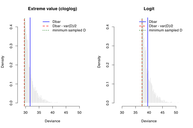
The histograms show why all four versions agree. The sampled deviance has a hard lower bound at its value at the mode and a right skew — approximately \(D(\widehat{\boldsymbol{\beta}}) + \chi^2_2\) — and the estimated \(\widehat{D}\) lands right at the bottom edge of the distribution in both cases.
(f) The logit link.
tabL <- dic.table(fitL$sims, 'logit'); colnames(tabL) <- colnames.dic
round(tabL, 3)
round(tabL[, 'DIC'] - tabF[, 'DIC'], 3)
Dbar Dhat pD DIC
DIC (R2WinBUGS) 39.494 37.398 2.095 41.589
Mean of beta 39.494 37.444 2.050 41.544
Median of beta 39.494 37.437 2.057 41.551
Half variance of D(.) 39.494 37.398 2.095 41.589
DIC (R2WinBUGS) Mean of beta Median of beta
7.725 7.809 7.813
Half variance of D(.)
7.725
Which link fits best? The extreme-value link, decisively. Its DIC is about \(33.8\) against about \(41.6\) for the logit, a difference of \(7.7\) to \(7.8\).
Was the difference consistent across methods? Yes, completely. Every one of the four ways of computing \(\widehat{D}\) gives a DIC difference between \(7.72\) and \(7.81\) — a spread of \(0.09\), versus a signal of \(7.8\). The choice of estimator affects the third significant figure of the DIC and has no bearing at all on the model comparison. That is the reassuring finding: the ambiguity in defining \(p_D\) matters far less than the difference between the models.
The comparison also passes an external check. \(p_D \approx 2\) in both models, so DIC here is essentially \(\bar{D} + 2 \approx D(\widehat{\boldsymbol{\beta}}) + 2 \times 2\), the AIC. And indeed the classical AICs are \(33.64\) (cloglog) and \(41.43\) (logit), within \(0.25\) of every DIC in the two tables. With vague priors and a well-behaved two-parameter model, DIC reduces to AIC, exactly as Section 13.6 says it should.
On the guideline in Section 13.6 — differences below 5 small, above 10 substantial — a gap of \(7.8\) sits in the intermediate zone, so the formally correct statement is that the extreme-value link is clearly preferred but the evidence is strong rather than overwhelming. The substantive reason to prefer it, established in Exercise 13.3(c) and (k), is that the observed dose–response curve is asymmetric and the logit link cannot be.
(g) When might the DIC not work well? The calculations above worked because this problem is about as benign as a Bayesian model gets: two parameters, a unimodal near-Normal posterior, a nearly quadratic deviance, vague priors, and a converged chain. Each of those conditions is a potential failure point.
- Multimodal or badly skewed posteriors. Section 13.6 makes this point explicitly. If the deviance has several minima, \(\overline{\boldsymbol{\beta}}\) can fall between the modes in a region of low posterior density and high deviance, so \(D(\overline{\boldsymbol{\beta}})\) is not the smallest attainable deviance. Then \(p_D\) from Equation (13.5) is too small, or even negative, and the DIC is not measuring model fit. Mixture models with label switching are the standard pathology.
- Non-invariance to parameterisation. \(\overline{\boldsymbol{\beta}}\) is not invariant to reparameterisation: the mean of \(\log\sigma\) is not the log of the mean of \(\sigma\). Fitting the same model in two algebraically equivalent parameterisations can produce two different values of \(D(\overline{\boldsymbol{\beta}})\), hence two different \(p_D\) and DIC. Exercise 13.3(g) is a direct illustration that reparameterisation is routine in MCMC practice. The half-variance version of \(p_D\) avoids this, which is another argument in its favour.
- Dependence on the parameter space and priors. Also flagged in Section 13.6: informative priors, or priors that restrict the parameter space, change the effective number of parameters and hence the DIC. Two models can only be compared by DIC if their priors are comparable, and DIC is not a legitimate way to compare models with genuinely different prior structures.
- Ambiguity about what counts as a parameter (the “focus” problem). In a hierarchical or multilevel model such as the random intercept of Section 11.5, the deviance can be defined conditionally on the random effects or with them integrated out. The two choices give different \(p_D\) and different DIC, and neither is canonically correct. In practice the conditional form is what WinBUGS reports, and it answers a question about predicting new observations within existing groups, not new groups.
- Unconverged or poorly mixing chains. All the DIC quantities are Monte Carlo averages. Exercise 13.3(f) produced a chain whose deviance was still falling after 10,000 iterations; its \(\bar{D}\) was \(66.4\) instead of \(31.7\) and its \(D(\overline{\boldsymbol{\beta}})\) would be nonsense. The DIC is only as good as the chain, and it carries no warning label when the chain is bad. The half-variance \(p_D\) is especially fragile, because a variance needs many more effective samples to estimate than a mean.
- Missing data and latent variables. When missing values are imputed as part of the MCMC, “the data” \(\mathbf{y}\) differ from iteration to iteration and the deviance is not comparable across iterations, so \(\bar{D}\) is not meaningful.
- Non-exponential-family or non-standard likelihoods. \(D = -2\log p(\mathbf{y} \mid \boldsymbol{\theta})\) includes the normalising constant. Comparing models with different likelihood families is safe only if that constant is retained consistently in both — and it is meaningless to compare a model for counts with a model for the log of the counts.
- Small samples. The asymptotic argument that ties \(p_D\) to the number of parameters is a large-sample one. With \(N = 8\) dose groups it worked here, but that is partly luck; with few observations relative to parameters the DIC’s penalty is not reliably calibrated.
The practical summary is the one Section 13.6 gives: DIC is a guide, not a decision rule. Check the deviance trace for convergence first, compute \(p_D\) both ways and be suspicious if they disagree or if \(p_D\) is far from the number of fitted parameters, and treat differences below about 5 as inconclusive.
Example Bayesian Analyses
Problem 14.1 — Confirm that setting \(\varphi\)1 = 1 in model (14.1) gives model (8.11).
Confirm that setting \(\phi_1 = 1\) in model (14.1) gives model (8.11). (difficulty: \(\star\))
Model (14.1) is the WinBUGS parameterisation of the nominal logistic regression used in Section 14.3. It introduces non-negative quantities \(\phi_1,\phi_2,\phi_3\) and writes
\[ \log(\phi_j) \;=\; \beta_{0j} + \beta_{1j}x_1 + \beta_{2j}x_2 + \beta_{3j}x_3, \qquad j = 2,3, \]
\[ \pi_j \;=\; \frac{\phi_j}{\sum_{k=1}^{3}\phi_k}, \qquad j = 1,2,3 . \]
The book’s model (8.11) is the classical nominal logistic regression for the car preference data with “no or little importance” as the reference category,
\[ \log\left(\frac{\pi_j}{\pi_1}\right) \;=\; \beta_{0j} + \beta_{1j}x_1 + \beta_{2j}x_2 + \beta_{3j}x_3, \qquad j = 2,3 . \]
Why a constraint is needed. The map \(\boldsymbol{\phi}\mapsto\boldsymbol{\pi}\) is invariant to rescaling: for any \(c>0\), replacing \(\phi_k\) by \(c\phi_k\) for every \(k\) leaves each \(\pi_j = c\phi_j/\sum_k c\phi_k\) unchanged. So \(\boldsymbol{\phi}\) is identified only up to a positive multiple, and exactly one normalising restriction is needed. Fixing \(\phi_1 = 1\) is one such restriction (equivalently, taking \(c = 1/\phi_1\)), and it costs nothing: any \(\boldsymbol{\phi}\) with \(\phi_1>0\) can be rescaled to satisfy it without changing \(\boldsymbol{\pi}\).
The derivation. Take the ratio of \(\pi_j\) to \(\pi_1\). The normalising sum \(\sum_{k}\phi_k\) is common to numerator and denominator and cancels:
\[ \frac{\pi_j}{\pi_1} \;=\; \frac{\phi_j / \sum_{k=1}^{3}\phi_k}{\phi_1 / \sum_{k=1}^{3}\phi_k} \;=\; \frac{\phi_j}{\phi_1}. \]
Now impose \(\phi_1 = 1\), so that \(\pi_j/\pi_1 = \phi_j\) and
\[ \log\left(\frac{\pi_j}{\pi_1}\right) \;=\; \log(\phi_j) \;=\; \beta_{0j} + \beta_{1j}x_1 + \beta_{2j}x_2 + \beta_{3j}x_3, \qquad j = 2,3, \]
which is precisely (8.11). This is the line phi[i,1]<-1; # For identifiability in the WinBUGS code of Section 14.3.
Consistency at \(j=1\). Model (8.11) is stated only for \(j=2,3\) because the \(j=1\) equation is degenerate: \(\log(\pi_1/\pi_1) = 0\). Under (14.1) the same holds automatically, since \(\log(\phi_1)=\log 1 = 0\); the constraint \(\phi_1=1\) is therefore the statement that all four regression coefficients for the reference category are zero, \(\beta_{01}=\beta_{11}=\beta_{21}=\beta_{31}=0\), which is exactly the corner-point constraint that makes category 1 the reference in (8.11).
Recovering the probabilities. Inverting, with \(\phi_1=1\),
\[ \pi_1 = \frac{1}{1 + \phi_2 + \phi_3}, \qquad \pi_j = \frac{\phi_j}{1 + \phi_2 + \phi_3} \;\;(j=2,3), \]
so \(\pi_1+\pi_2+\pi_3 = 1\) by construction and each \(\pi_j > 0\) because \(\phi_j = \exp(\cdot) > 0\). The parameterisation therefore enforces the multinomial constraints automatically, which is the practical reason for using it in WinBUGS: the \(\phi_j\) are unconstrained on the log scale, so vague Normal priors can be put on the \(\beta\)’s without any risk of proposing a \(\boldsymbol{\pi}\) outside the simplex. This is the same device as the “\(\pi_j = \phi_j/\sum\phi_k\)” construction used on page 186 of Section 8.3.
A numerical confirmation using the Table 14.5 posterior means for the reference cell, women aged 18–23, where \(x_1=x_2=x_3=0\) so that \(\phi_2 = e^{-0.602}\) and \(\phi_3 = e^{-1.063}\).
b02 <- -0.602; b03 <- -1.063
phi <- c(1, exp(b02), exp(b03))
pi.hat <- phi / sum(phi)
round(pi.hat, 4)
round(log(pi.hat[2:3] / pi.hat[1]), 4) # should return b02, b03
[1] 0.5282 0.2893 0.1825
[1] -0.602 -1.063
So the reference cell (women aged 18–23) has fitted preference probabilities \((0.53, 0.29, 0.18)\) for “no or little”, “important” and “very important”, and the log ratios return the two constants exactly, as required.
Problem 14.2 — Prove that the latent variable model (14.2) is equal to the proportional odds
Prove that the latent variable model (14.2) is equal to the proportional odds model (8.17). (difficulty: \(\star\star\))
Set-up. The latent variable formulation of Section 14.4 supposes an unobserved continuous response \(z\) and ordered cutpoints \(C_1 < C_2 < \dots < C_{J-1}\); the observed ordinal category is \(j\) when \(C_{j-1} < z \le C_j\) (with \(C_0 = -\infty\), \(C_J = +\infty\)). Writing
\[ Q_j \;=\; P(z > C_j), \qquad j = 1,\dots,J-1, \]
model (14.2) is
\[ \log\left(\frac{Q_j}{1-Q_j}\right) \;=\; \log\left(\frac{P(z > C_j)}{P(z \le C_j)}\right) \;=\; \mathbf{x}^{T}\boldsymbol{\beta} - C_j . \]
The crucial feature is that \(\boldsymbol{\beta}\) carries no \(j\) subscript: the same slope vector appears for every cutpoint, and only the intercept \(-C_j\) changes with \(j\).
Translating \(Q_j\) into cumulative probabilities. Since category \(j\) is the event \(C_{j-1} < z \le C_j\), we have \(\pi_j = P(C_{j-1} < z \le C_j)\) and hence, telescoping,
\[ P(z \le C_j) \;=\; \sum_{k=1}^{j}\pi_k \;=\; \pi_1 + \dots + \pi_j, \qquad P(z > C_j) \;=\; \pi_{j+1} + \dots + \pi_J . \]
(This also reproduces the probability formulae printed in Section 14.4: \(\pi_1 = 1-Q_1\), \(\pi_j = Q_{j-1}-Q_j\) for \(j=2,\dots,J-1\), and \(\pi_J = Q_{J-1}\).) Therefore
\[ \frac{Q_j}{1-Q_j} \;=\; \frac{\pi_{j+1} + \dots + \pi_J}{\pi_1 + \dots + \pi_j}, \]
which is the reciprocal of the odds used in the proportional odds model (8.14).
The equivalence. Substituting into (14.2) and negating both sides,
\[ \log\left(\frac{\pi_{j+1} + \dots + \pi_J}{\pi_1 + \dots + \pi_j}\right) \;=\; \mathbf{x}^{T}\boldsymbol{\beta} - C_j \quad\Longleftrightarrow\quad \log\left(\frac{\pi_1 + \dots + \pi_j}{\pi_{j+1} + \dots + \pi_J}\right) \;=\; C_j - \mathbf{x}^{T}\boldsymbol{\beta} . \]
The right-hand side is a linear predictor whose intercept depends on \(j\) and whose slopes do not, so this is exactly the proportional odds model (8.14),
\[ \log\left(\frac{\pi_1 + \dots + \pi_j}{\pi_{j+1} + \dots + \pi_J}\right) \;=\; \beta_{0j}^{\ast} + \beta_1^{\ast}x_1 + \dots + \beta_{p-1}^{\ast}x_{p-1}, \]
under the correspondence
\[ \beta_{0j}^{\ast} \;=\; C_j - \beta_0, \qquad \beta_k^{\ast} \;=\; -\beta_k \quad (k = 1,\dots,p-1), \]
where \(\beta_0\) is the constant term inside \(\mathbf{x}^{T}\boldsymbol{\beta}\). For the car preference data \(J=3\), \(\mathbf{x}^{T}\boldsymbol{\beta} = \beta_0 + \beta_1x_1 + \beta_2x_2 + \beta_3x_3\) with \(x_1,x_2,x_3\) the sex and age dummies of (8.11), and the two equations are
\[ \log\left(\frac{\pi_1}{\pi_2+\pi_3}\right) = C_1 - \beta_0 - \beta_1x_1 - \beta_2x_2 - \beta_3x_3, \qquad \log\left(\frac{\pi_1+\pi_2}{\pi_3}\right) = C_2 - \beta_0 - \beta_1x_1 - \beta_2x_2 - \beta_3x_3, \]
which is model (8.17) with \(\beta_{01}^{\ast} = C_1-\beta_0\) and \(\beta_{02}^{\ast} = C_2-\beta_0\).
Two remarks on identifiability and sign.
- The constant \(\beta_0\) and the cutpoints are confounded: only the differences \(C_j-\beta_0\) are estimable, which is why the WinBUGS code of Section 14.4 fixes \(C_1 \leftarrow 0\) and lets
beta[1]absorb the location. The ordering constraint \(C_1<C_2<\dots<C_{J-1}\) is what guarantees \(Q_1 > Q_2 > \dots\), i.e. that the fitted \(\pi_j\) are non-negative; it is enforced by the nested Uniform priors \(C_j \sim U[C_{j-1},C_{j+1}]\). - The slopes carry opposite signs in the two orientations. In (14.2) a positive \(\beta_k\) raises \(P(z > C_j)\) for every \(j\), so \(\exp(\beta_k)\) is the odds ratio for being in a higher category, exactly as Table 14.6 describes it; the derivation above puts \(-\beta_k\) in front of \(x_k\) on the “lower category” side. Worth flagging that Dobson’s Table 8.4 is nevertheless numerically identical in sign to Table 14.6 (\(\beta_1 = -0.576\) against \(-0.580\), \(\beta_2 = 1.147\) against \(1.162\), \(\beta_3 = 2.232\) against \(2.258\)). The reason is that Table 8.4 reports the output of
polr, which parameterises the cumulative model as \(\mathrm{logit}\,P(Y \le j) = \zeta_j - \mathbf{x}^{T}\boldsymbol{\eta}\), i.e. with the minus sign already built in. So (8.17) as printed, with \(+\beta_kx_k\) on the lower-category side, does not quite match the signs of the estimates tabulated beneath it; the latent variable orientation of (14.2) is the one that Table 8.4 actually uses. The two model families are the same either way, and the fitted \(\pi_j\) are identical.
The equivalence is verified numerically below. Reconstructing the fitted probabilities from the latent-variable formulae of Section 14.4, \(Q_j = \mathrm{expit}(\mathbf{x}^{T}\boldsymbol{\beta}-C_j)\) with \(C_j = \zeta_j\), reproduces polr’s own fitted values to machine precision.
library(MASS)
sex <- rep(c("women","men"), each = 3)
age <- rep(c("18-23","24-40",">40"), 2)
freq <- rbind(c(26,12,7), c(9,21,15), c(5,14,41),
c(40,17,8), c(17,15,12), c(8,15,18))
d <- data.frame(sex = factor(sex, levels = c("women","men")),
age = factor(age, levels = c("18-23","24-40",">40")))
long <- d[rep(1:6, times = rowSums(freq)), ]
long$resp <- factor(unlist(apply(freq, 1, function(r) rep(1:3, r))),
levels = 1:3, ordered = TRUE)
fit <- polr(resp ~ sex + age, data = long, Hess = TRUE)
round(c(coef(fit), fit$zeta), 4)
# rebuild pi from the latent-variable model (14.2): Q_j = expit(x'beta - C_j)
X <- model.matrix(~ sex + age, data = d)[, -1, drop = FALSE]
xb <- as.vector(X %*% coef(fit))
Q <- sapply(fit$zeta, function(C) plogis(xb - C))
pr <- cbind(1 - Q[, 1], Q[, 1] - Q[, 2], Q[, 2])
round(pr, 4)
max(abs(pr - predict(fit, newdata = d, type = "probs")))
sexmen age24-40 age>40 1|2 2|3
-0.5762 1.1471 2.2325 0.0435 1.6550
[,1] [,2] [,3]
[1,] 0.5109 0.3287 0.1604
[2,] 0.2491 0.3752 0.3757
[3,] 0.1007 0.2588 0.6405
[4,] 0.6502 0.2529 0.0970
[5,] 0.3711 0.3761 0.2527
[6,] 0.1662 0.3335 0.5003
[1] 1.110223e-16
Three checks pass at once. The cutpoints \(\hat C_1 = 0.044\) and \(\hat C_2 = 1.655\) are exactly the intercepts \(\beta_{01}\), \(\beta_{02}\) printed in Table 8.4, and the reconstructed probabilities for the reference cell, \((0.5109, 0.3287, 0.1604)\), are exactly the values Dobson quotes for females aged 18–23 in Section 8.4.6. The slopes \((-0.576, 1.147, 2.232)\) match the WinBUGS latent variable posterior means in Table 14.6 (\(-0.580\), \(1.162\), \(2.258\)) to within Monte Carlo error. So the Bayesian latent variable model and the classical proportional odds model are the same model, fitted by different algorithms.
Problem 14.3 — a. Run the Weibull model for the remission times survival data, but this
a. Run the Weibull model for the remission times survival data, but this time monitor the DIC.
b. Create an exponential model for the remission times in WinBUGS. Monitor the DIC. Is the exponential model a better model than the Weibull? Compare the results with Section 10.7. (difficulty: \(\star\star\))
WinBUGS is not available here, so both models are fitted with a random walk Metropolis sampler written directly in R. This is not a workaround for its own sake: writing the sampler makes the likelihood, the priors and the DIC arithmetic completely explicit, and the posterior summaries below reproduce Table 14.7 to within Monte Carlo error, which is the check that the substitution is legitimate.
The two models. Following the WinBUGS code of Section 14.5, survival time \(y_i\) for patient \(i\) has a Weibull distribution with shape \(\lambda\) and scale parameter \(\phi_i\), so that the survivor and density functions are
\[ S(y_i) = \exp\left(-\phi_i y_i^{\lambda}\right), \qquad f(y_i) = \lambda\phi_i y_i^{\lambda-1}\exp\left(-\phi_i y_i^{\lambda}\right), \qquad \log\phi_i = \beta_0 + \beta_1 x_i, \]
with \(x_i = 1\) for the 6-mercaptopurine group and \(0\) for the control group. The hazard is \(h(y) = \lambda y^{\lambda-1}\exp(\beta_0+\beta_1 x)\), which is exactly the Weibull proportional hazards model of Section 10.7, so \(\beta_0\), \(\beta_1\) and \(\lambda\) are directly comparable with Table 10.3. Setting \(\lambda = 1\) gives the exponential model \(h(y) = \exp(\beta_0+\beta_1 x)\).
With \(\delta_i = 1\) for an observed remission and \(\delta_i = 0\) for a right-censored time, the observed-data log-likelihood is
\[ \ell = \sum_{i=1}^{42}\Big[\delta_i\big\{\log\lambda + \log\phi_i + (\lambda-1)\log y_i\big\} - \phi_i y_i^{\lambda}\Big], \]
the censored observations contributing \(\log S(y_i) = -\phi_i y_i^{\lambda}\) only. The priors are those in the book’s code: \(\beta_0,\beta_1 \sim N(0,1000)\) and \(\lambda \sim \mathrm{Exp}(0.001)\). Sampling is done on \(\log\lambda\) (with the Jacobian term added) so that all three parameters live on the whole line.
One difference from WinBUGS should be stated plainly. WinBUGS treats a censored time as missing data drawn from a truncated Weibull, so its deviance is computed on an augmented likelihood; the sampler here uses the standard observed-data likelihood with \(S(y_i)\) for censored cases. The posteriors for \(\beta_0,\beta_1,\lambda\) are identical in either formulation (the censored times are integrated out analytically rather than imputed), but the absolute level of the deviance, and hence the numerical value of DIC, differs from what WinBUGS reports. Since both models here are scored on the same likelihood, the comparison of DICs, which is what the question asks for, is unaffected.
(a) Weibull model with DIC.
library(dobson)
data(remission)
y <- remission$time
d <- as.numeric(remission$censored == 0) # 1 = remission observed
x <- as.numeric(remission$group == "T") # 1 = 6-MP treatment
loglik <- function(p, weib = TRUE) { # p = c(beta0, beta1, log lambda)
lam <- if (weib) exp(p[3]) else 1
lphi <- p[1] + p[2] * x
sum(d * (log(lam) + lphi + (lam - 1) * log(y)) - exp(lphi) * y^lam)
}
logpost <- function(p, weib = TRUE) {
lp <- loglik(p, weib) + sum(dnorm(p[1:2], 0, sqrt(1000), log = TRUE))
if (weib) lp <- lp + dexp(exp(p[3]), 0.001, log = TRUE) + p[3]
lp
}
mcmc <- function(weib, init, sd.prop, n.burn = 5000, n.keep = 20000, seed = 1) {
set.seed(seed)
k <- if (weib) 3 else 2
cur <- init; lc <- logpost(cur, weib); out <- matrix(NA, n.keep, k)
for (it in 1:(n.burn + n.keep)) {
prop <- cur + rnorm(k, 0, sd.prop)
lp <- logpost(prop, weib)
if (log(runif(1)) < lp - lc) { cur <- prop; lc <- lp }
if (it > n.burn) out[it - n.burn, ] <- cur
}
out
}
rhat <- function(ch) sapply(seq_len(ncol(ch[[1]])), function(j) {
xs <- sapply(ch, function(z) z[, j]); n <- nrow(xs)
W <- mean(apply(xs, 2, var)); B <- n * var(colMeans(xs))
sqrt(((n - 1) / n * W + B / n) / W)
})
ch <- lapply(1:2, function(s) mcmc(TRUE, c(-3, -1.7, log(1.4)),
c(0.35, 0.35, 0.11), seed = s))
W <- rbind(ch[[1]], ch[[2]]); W[, 3] <- exp(W[, 3])
colnames(W) <- c("beta0", "beta1", "lambda")
round(t(apply(W, 2, function(z)
c(mean = mean(z), sd = sd(z), quantile(z, c(.025, .975))))), 3)
round(rhat(ch), 4)
mean sd 2.5% 97.5%
beta0 -3.141 0.587 -4.366 -2.031
beta1 -1.774 0.425 -2.674 -0.990
lambda 1.383 0.210 0.992 1.819
[1] 1.0018 1.0005 1.0014
The Gelman–Rubin statistics are all essentially 1, so the two chains have converged. The posterior means reproduce Table 14.7 closely: the book reports \(\beta_1 = -1.778\) (\(-2.64\), \(-0.978\)), \(\beta_0 = -3.162\) (\(-4.349\), \(-2.145\)) and \(\lambda = 1.39\) (\(1.023\), \(1.802\)).
The median survival times and their difference, the quantities the book highlights as a particular advantage of the Bayesian fit, follow from \(\mathrm{median} = \{\log 2 \cdot \exp(-\log\phi)\}^{1/\lambda}\) applied to every retained draw.
med.c <- (log(2) * exp(-W[, 1]))^(1 / W[, 3])
med.t <- (log(2) * exp(-(W[, 1] + W[, 2])))^(1 / W[, 3])
M <- cbind(control = med.c, treatment = med.t, difference = med.t - med.c)
round(t(apply(M, 2, function(z) c(mean = mean(z), quantile(z, c(.025, .975))))), 3)
mean 2.5% 97.5%
control 7.463 4.904 10.477
treatment 27.935 17.113 47.693
difference 20.473 9.121 40.772
Again this matches Table 14.7 (\(7.538\), \(27.65\), difference \(20.11\) with interval \(9.367\) to \(38.12\)). Median remission time under 6-MP is roughly 28 weeks against 7.5 weeks for the controls, an extension of about 20 weeks whose 95% posterior interval excludes zero comfortably.
The DIC of Section 13.6 is \(\mathrm{DIC} = \bar{D} + p_D\) where \(D(\boldsymbol{\theta}) = -2\ell(\boldsymbol{\theta})\), \(\bar{D}\) is its posterior mean and \(p_D = \bar{D} - D(\bar{\boldsymbol{\theta}})\).
dic <- function(S, weib) {
tr <- function(p) if (weib) c(p[1], p[2], log(p[3])) else p
D <- -2 * apply(S, 1, function(p) loglik(tr(p), weib))
Dbar <- mean(D); Dhat <- -2 * loglik(tr(colMeans(S)), weib)
c(Dbar = Dbar, Dhat = Dhat, pD = Dbar - Dhat, DIC = Dbar + (Dbar - Dhat))
}
round(dic(W, TRUE), 2)
Dbar Dhat pD DIC
216.33 213.21 3.12 219.45
The estimated number of parameters \(p_D = 3.12\) is essentially the actual number, three, which is what one expects with 42 observations, vague priors and a well-identified likelihood.
(b) Exponential model with DIC. Setting \(\lambda \equiv 1\) removes one parameter; the sampler and the DIC function are reused unchanged.
che <- lapply(1:2, function(s) mcmc(FALSE, c(-2.2, -1.5), c(0.22, 0.42), seed = 10 + s))
E <- rbind(che[[1]], che[[2]]); colnames(E) <- c("beta0", "beta1")
round(t(apply(E, 2, function(z)
c(mean = mean(z), sd = sd(z), quantile(z, c(.025, .975))))), 3)
round(rhat(che), 4)
mec <- log(2) * exp(-E[, 1]); met <- log(2) * exp(-(E[, 1] + E[, 2]))
ME <- cbind(control = mec, treatment = met, difference = met - mec)
round(t(apply(ME, 2, function(z) c(mean = mean(z), quantile(z, c(.025, .975))))), 3)
round(dic(E, FALSE), 2)
mean sd 2.5% 97.5%
beta0 -2.188 0.217 -2.636 -1.787
beta1 -1.556 0.404 -2.380 -0.794
[1] 1.0000 1.0004
mean 2.5% 97.5%
control 6.332 4.141 9.677
treatment 31.183 15.677 60.791
difference 24.851 8.945 54.360
Dbar Dhat pD DIC
219.07 217.09 1.98 221.05
Is the exponential model better? No, but only just. The DIC falls from \(221.05\) (exponential) to \(219.45\) (Weibull), a change of \(1.6\). A difference of this size is conventionally regarded as inconsequential; the two models are essentially indistinguishable in fit. The Weibull buys its slightly better fit with \(p_D = 3.12\) against \(1.98\) effective parameters, so the extra shape parameter is doing very little work. That is consistent with the posterior for \(\lambda\): its mean is \(1.383\) but its 95% interval, \((0.992, 1.819)\), only barely excludes \(\lambda = 1\), so the data do not insist on a non-constant hazard.
Comparison with Section 10.7. The classical fits are reproduced below.
library(survival)
we <- survreg(Surv(time, censored == 0) ~ group, dist = "weibull", data = remission)
ex <- survreg(Surv(time, censored == 0) ~ group, dist = "exponential", data = remission)
c(lambda = 1 / we$scale, beta0 = -coef(we)[1] / we$scale, beta1 = -coef(we)[2] / we$scale)
c(beta0 = -coef(ex)[1], beta1 = -coef(ex)[2])
c(AIC.weibull = AIC(we), AIC.exponential = AIC(ex))
lambda beta0.(Intercept) beta1.groupT
1.365758 -3.070704 -1.730872
beta0.(Intercept) beta1.groupT
-2.159484 -1.526614
AIC.weibull AIC.exponential
219.1590 221.0481
The maximum likelihood estimates \(\lambda = 1.366\), \(\beta_0 = -3.071\), \(\beta_1 = -1.731\) are exactly the values in the last row of Table 10.3, and the exponential estimates \(\beta_0 = -2.159\), \(\beta_1 = -1.527\) match the first row. The Bayesian posterior means sit very slightly further from zero than the MLEs (\(\beta_1 = -1.774\) against \(-1.731\)), the usual mild effect of averaging over a right-skewed likelihood rather than maximising it, and the posterior for \(\lambda\) is centred a little above the MLE for the same reason. The Bayesian standard deviations for the Weibull \(\beta\)’s are honest, whereas Section 10.7 explicitly warns that the Poisson-regression standard errors for the Weibull model are too small because they ignore the uncertainty in \(\hat\lambda\).
The one place where the Bayesian and classical conclusions appear to diverge is model choice. Section 10.7 states AIC \(= 2.429\) for the exponential and \(2.782\) for the Weibull and prefers the exponential. Those numbers are not AIC on the usual scale: they are the AIC of the Poisson regression surrogate divided by \(n = 42\). The exponential surrogate is glm(censored = 0 ~ group + offset(log(time)), family = poisson())=, whose \(\mathrm{AIC}/n = 102.017/42 = 2.429\); the Weibull surrogate uses the offset \(\hat\lambda\log(y)\) and gives \(116.84/42 = 2.782\). Because the two surrogate fits use different offsets, their Poisson log-likelihoods contain different data-dependent constants and the two AIC values are not on a common scale, so the ordering they produce is not evidence about the survival models. On the proper survival likelihood the AIC values are \(219.16\) (Weibull) and \(221.05\) (exponential), a difference of \(1.9\) in favour of the Weibull, which agrees in both direction and magnitude with the DIC difference of \(1.6\).
So the honest summary is the one Dobson reaches anyway, by a route that happens not to support it: the exponential distribution is about as good as the Weibull for these data, the shape parameter is only marginally distinguishable from 1, and the exponential model would be chosen on grounds of parsimony and interpretability, its relative hazard \(\exp(1.556) = 4.74\) (posterior mean; \(\exp(1.527)=4.60\) classically) saying that the control group relapses at roughly four and a half times the rate of the treated group at every time point.
Problem 14.4 — a. Fit the random intercepts and slopes model to the stroke recovery data
a. Fit the random intercepts and slopes model to the stroke recovery data in WinBUGS. Create a scatter plot of the estimated mean random slopes against the random intercepts. Calculate the Pearson correlation between the intercepts and slopes.
b. Model the random slopes and intercepts so that each subject’s intercept is correlated with his or her slope (using a multivariate Normal distribution). Find the mean and 95% posterior interval for the correlation between the intercept and slope. Interpret the correlation and give reasons for the somewhat surprising value.
Hint: To start the MCMC sampling, it may be necessary to use initial values based on the means of the random intercepts and slopes model from part (a). (difficulty: \(\star\star\star\))
The model of Section 14.6 for the stroke recovery data (Table 11.1) is
\[ Y_{jt} = \alpha_g + a_j + (\beta_g + b_j)t + e_{jt}, \qquad j=1,\dots,24,\; t=1,\dots,8,\; g=1,2,3, \]
with \(e_{jt} \sim N(0,\sigma_e^2)\). Part (a) takes \(a_j \sim N(0,\sigma_a^2)\) and \(b_j \sim N(0,\sigma_b^2)\) independently; part (b) replaces this by \((a_j,b_j)^T \sim \mathrm{MVN}(\mathbf{0},\mathbf{G})\) with an unstructured \(2\times 2\) matrix \(\mathbf{G}\).
In place of WinBUGS a Gibbs sampler is written directly in R. Every full conditional here is available in closed form, which makes this straightforward and fast: the fixed effects \((\alpha_1,\alpha_2,\alpha_3,\beta_1,\beta_2,\beta_3)\) given everything else are a Normal linear model on the residuals \(y-\mathbf{Z}\mathbf{u}\); each pair \((a_j,b_j)\) given everything else is bivariate Normal; the Uniform prior \(\sigma_e^2 \sim U(0,10^4)\) used in the book’s code makes the conditional for \(\sigma_e^2\) an inverse gamma with shape \(n/2-1\) (the truncation at \(10^4\) is never binding and is ignored); the same holds for \(\sigma_a^2\) and \(\sigma_b^2\) in part (a); and in part (b) the Wishart prior \(\mathbf{G}^{-1}\sim W(\mathbf{R},\nu)\) is conjugate, giving \(\mathbf{G}^{-1}\mid\cdot \sim W\big((\mathbf{R}+\sum_j \mathbf{u}_j\mathbf{u}_j^T)^{-1},\,\nu+N\big)\) in the scale-matrix convention rWishart uses. Following the hint, part (b) is started from the part (a) values. Time is entered as \(t=1,\dots,8\) and the responses are left on their original scale (the book’s centring at 50 is only a convergence device for WinBUGS and is not needed here).
(a) Independent random intercepts and slopes.
library(dobson)
data(stroke.wide)
Y <- as.matrix(stroke.wide[, paste0("week", 1:8)])
N <- nrow(Y); T <- ncol(Y); tt <- 1:T
grp <- as.integer(factor(stroke.wide$Group))
y <- as.vector(t(Y)); subj <- rep(1:N, each = T); tidx <- rep(1:T, N)
g <- grp[subj]; time <- tt[tidx]
X <- cbind(outer(g, 1:3, "==") * 1, outer(g, 1:3, "==") * time) # alphas then betas
Z <- cbind(1, tt); ZtZ <- crossprod(Z)
gibbs <- function(corr, n.burn = 2000, n.keep = 20000, seed = 1,
Rprior = diag(2), nu = 2) {
set.seed(seed); p <- ncol(X); XtX <- crossprod(X)
th <- as.vector(coef(lm(y ~ X - 1))); U <- matrix(0, N, 2)
s2 <- 100; G <- diag(c(400, 10))
keep.th <- matrix(NA, n.keep, p); keep.U <- matrix(0, N, 2)
keep.G <- matrix(NA, n.keep, 3); keep.s2 <- keep.rho <- numeric(n.keep)
for (it in 1:(n.burn + n.keep)) {
ystar <- y - rowSums(Z[tidx, ] * U[subj, ]) # fixed effects
V <- solve(XtX / s2 + diag(1e-4, p))
th <- as.vector(V %*% (crossprod(X, ystar) / s2) + t(chol(V)) %*% rnorm(p))
r <- y - as.vector(X %*% th) # random effects
Vu <- solve(ZtZ / s2 + solve(G)); Lu <- t(chol(Vu))
Mu <- Vu %*% (crossprod(Z, matrix(r, nrow = T)) / s2)
U <- t(Mu + Lu %*% matrix(rnorm(2 * N), 2, N))
e <- r - rowSums(Z[tidx, ] * U[subj, ]) # residual variance
s2 <- 1 / rgamma(1, length(y) / 2 - 1, sum(e^2) / 2)
if (corr) {
Wm <- solve(Rprior + crossprod(U))
G <- solve(rWishart(1, nu + N, (Wm + t(Wm)) / 2)[, , 1])
} else {
G <- diag(c(1 / rgamma(1, N / 2 - 1, sum(U[, 1]^2) / 2),
1 / rgamma(1, N / 2 - 1, sum(U[, 2]^2) / 2)))
}
if (it > n.burn) {
k <- it - n.burn; keep.th[k, ] <- th; keep.U <- keep.U + U / n.keep
keep.G[k, ] <- c(G[1, 1], G[2, 2], G[1, 2]); keep.s2[k] <- s2
keep.rho[k] <- G[1, 2] / sqrt(G[1, 1] * G[2, 2])
}
}
list(th = keep.th, U = keep.U, G = keep.G, s2 = keep.s2, rho = keep.rho)
}
sm <- function(z) c(mean = mean(z), sd = sd(z), quantile(z, c(.025, .975)))
nm <- c("alpha1", "alpha2", "alpha3", "beta1", "beta2", "beta3")
fa <- gibbs(FALSE, seed = 2)
o <- t(apply(fa$th, 2, sm)); rownames(o) <- nm; round(o, 3)
c(sigma.a = mean(sqrt(fa$G[, 1])), sigma.b = mean(sqrt(fa$G[, 2])),
sigma.e = mean(sqrt(fa$s2)))
mean sd 2.5% 97.5%
alpha1 29.896 8.099 12.854 45.498
alpha2 32.016 8.170 15.050 47.899
alpha3 29.205 8.349 12.509 45.077
beta1 6.349 1.150 4.017 8.548
beta2 4.230 1.130 1.992 6.483
beta3 3.569 1.213 1.022 5.877
sigma.a sigma.b sigma.e
22.716779 3.184529 5.254549
These reproduce the “Intercepts + slopes” row of Table 14.8 (\(\hat\alpha_1 = 30.38\) with s.d. \(7.988\), \(\hat\beta_1 = 6.378\) with s.d. \(1.207\)) and the book’s reported \(\hat\sigma_a = 22.4\) and \(\hat\sigma_b = 3.3\). Substantively, group A (the specialist stroke unit) improves by about 6.3 points per week, group B by 4.2 and group C by 3.6; the differences \(\hat\beta_2-\hat\beta_1 = -2.12\) and \(\hat\beta_3-\hat\beta_1 = -2.78\) have 95% intervals \((-5.23, 1.05)\) and \((-5.99, 0.52)\), so the advantage of group A is suggestive but not conclusive once between-subject variability in slopes is allowed for. The intercepts are indistinguishable across groups, consistent with randomisation.
The posterior mean random effects are plotted against each other, coded by treatment group.
par(mar = c(4.5, 4.5, 3, 1))
plot(fa$U[, 1], fa$U[, 2], pch = c(19, 17, 15)[grp],
col = c("black", "grey40", "grey65")[grp], cex = 1.5,
xlab = "random intercept a_j", ylab = "random slope b_j",
main = "Stroke recovery: posterior mean random effects (independent priors)")
abline(h = 0, v = 0, col = "grey80")
abline(lm(fa$U[, 2] ~ fa$U[, 1]), lwd = 2, lty = 2)
text(fa$U[, 1], fa$U[, 2], 1:N, pos = 4, cex = 0.75)
legend("topright", pch = c(19, 17, 15), col = c("black", "grey40", "grey65"),
legend = paste("Group", levels(factor(stroke.wide$Group))), bty = "n")
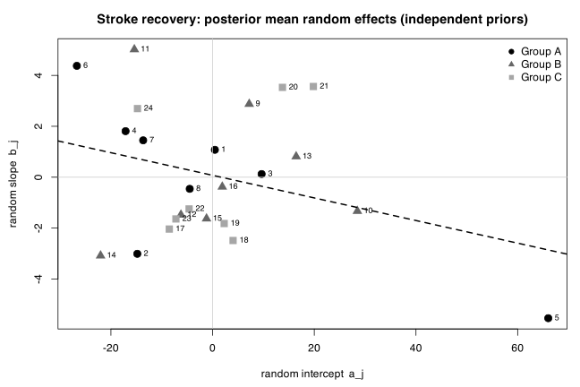
ct <- cor.test(fa$U[, 1], fa$U[, 2])
round(c(r = unname(ct$estimate), ct$conf.int, p = ct$p.value), 4)
r p
-0.3221 -0.6421 0.0935 0.1248
The Pearson correlation between the 24 posterior mean intercepts and the 24 posterior mean slopes is \(r = -0.32\) (95% confidence interval \(-0.64\) to \(0.09\), \(p = 0.12\)). Note that this is a correlation estimated after the fact from shrunken point estimates, under a model whose prior forced \(a_j\) and \(b_j\) to be independent; it is a descriptive summary, not an estimate of a model parameter, and it has no honest standard error because the 48 numbers being correlated are themselves posterior summaries. That is exactly why part (b) is needed.
The plot shows the pattern the correlation is picking up. Subject 5, far to the right and at the bottom, scored 100 at every one of the eight weeks: by far the largest random intercept, \(\hat a_5 = 66.0\), together with the most negative random slope, \(\hat b_5 = -5.5\), which cancels almost all of the group slope and leaves a fitted line that is essentially flat, because there is nowhere to go. Subject 21 and subject 20 combine high intercepts with high slopes, and subjects 6 and 11 combine low intercepts with the largest slopes.
(b) Correlated random effects. Now \((a_j,b_j)^T\sim\mathrm{MVN}(\mathbf{0},\mathbf{G})\) with \(\mathbf{G}^{-1}\sim W(\mathbf{R},\nu)\), \(\mathbf{R}=\mathbf{I}\) and \(\nu = 2\) (the smallest degrees of freedom for which the prior is proper in two dimensions), and the correlation \(\rho = G_{12}/\sqrt{G_{11}G_{22}}\) is monitored at every iteration.
fb <- gibbs(TRUE, seed = 3)
ob <- t(apply(fb$th, 2, sm)); rownames(ob) <- nm; round(ob, 3)
round(sm(fb$rho), 3)
c(sd.a = mean(sqrt(fb$G[, 1])), sd.b = mean(sqrt(fb$G[, 2])),
P.rho.neg = mean(fb$rho < 0))
mean sd 2.5% 97.5%
alpha1 29.770 7.304 15.118 44.491
alpha2 32.752 7.809 17.886 47.881
alpha3 29.354 7.606 14.759 44.941
beta1 6.437 1.042 4.423 8.491
beta2 4.322 1.105 2.093 6.538
beta3 3.611 1.075 1.515 5.817
mean sd 2.5% 97.5%
-0.355 0.192 -0.682 0.059
sd.a sd.b P.rho.neg
21.177021 2.953123 0.954600
The posterior mean correlation is \(\hat\rho = -0.36\) with 95% posterior interval \((-0.68, 0.06)\); \(P(\rho<0\mid\mathbf{y}) = 0.96\). Allowing the correlation barely changes the fixed effects, which is reassuring. The estimate is not an artefact of the Wishart prior: repeating with \(\nu = 4\), and with \(\mathbf{R}=\mathrm{diag}(500,10)\) chosen to be roughly on the scale of \(\mathbf{G}\), moves the posterior mean only between \(-0.33\) and \(-0.34\) with essentially the same interval.
Why the negative sign is surprising, and why it happens. The intuitive expectation is a positive correlation: patients who start off more able might be expected to recover faster too, and the two groups of numbers are both “how well is this patient doing”. Two mechanisms push the other way.
- The ceiling. The Barthel-type ability score is bounded above at 100. Ten of the 192 observations are exactly 100, spread over three subjects, and subject 5 sits at 100 for all eight weeks. A subject whose intercept is near the ceiling cannot have a large positive slope, so the top-right region of the plot is structurally empty and the fitted cloud tilts downwards. This is a genuine feature of the measurement scale, not of recovery.
- Where time zero is. This is the larger effect, and it is purely algebraic. The intercept \(\alpha_g+a_j\) is the fitted value at \(t=0\), a week before any data were collected. For a straight line fitted to \(x\)-values that are all positive, the estimated intercept and slope are negatively correlated by construction, with \(\mathrm{Cov}(\hat a,\hat b) = -\bar t\,\mathrm{Var}(\hat b)\): a line forced to be steeper must come down at \(t=0\) to keep passing through the data. Re-running exactly the same model with time centred at its mean, \(t^{\ast} = t - 4.5\), so that the intercept is the fitted value in the middle of the study, reverses the sign.
tt <- (1:8) - 4.5; time <- tt[tidx]
X <- cbind(outer(g, 1:3, "==") * 1, outer(g, 1:3, "==") * time)
Z <- cbind(1, tt); ZtZ <- crossprod(Z)
fc <- gibbs(TRUE, n.keep = 10000, seed = 5)
round(sm(fc$rho), 3)
# same thing seen in the raw per-subject least squares lines
raw <- t(apply(Y, 1, function(r) coef(lm(r ~ I(1:8)))))
cen <- t(apply(Y, 1, function(r) coef(lm(r ~ I((1:8) - 4.5)))))
round(c(time.from.zero = cor(raw[, 1], raw[, 2]),
time.centred = cor(cen[, 1], cen[, 2])), 3)
mean sd 2.5% 97.5%
0.269 0.204 -0.162 0.630
time.from.zero time.centred
-0.375 0.321
With the intercept defined at week 4.5 the posterior mean correlation is \(+0.27\) \((-0.16, 0.63)\), and the same flip is visible in the crudest possible summary, the ordinary least squares line fitted separately to each subject’s eight scores: \(r = -0.375\) with time measured from zero, \(r = +0.321\) with time centred.
So the correct interpretation is this. Patients who were doing better in the middle of the study did tend to be improving somewhat faster, but the effect is weak and its interval includes zero. The negative correlation reported by the model as specified is mostly telling us about the parameterisation rather than about stroke recovery: it says that a subject’s extrapolated week-zero ability and their rate of improvement trade off against each other, which is a property of fitting lines, reinforced by the ceiling on the score. This is the standard warning about interpreting the intercept-slope correlation in a random coefficients model: it is not invariant to where the time origin is placed, so it is only interpretable once the origin has been put somewhere meaningful.
Problem 14.5 — This exercise illustrates the effect of the choice of the Wishart prior for the
This exercise illustrates the effect of the choice of the Wishart prior for the unstructured covariance matrix using the stroke recovery data.
a. Fit a simple linear regression model to the stroke recovery data with terms for treatment and treatment by time. Store the residuals. Use either Bayesian or classical methods to fit the model.
b. Adapt the WinBUGS code for the AR(1) covariance pattern model to an unstructured covariance.
c. Run the model using a vague Wishart prior defined by \(\mathbf{R} = \hat\sigma^2\mathbf{I}\) and \(\nu = 9\). \(\mathbf{I}\) is the \(8 \times 8\) identity matrix and \(\hat\sigma^2\) is the variance of the residuals from part (a).
d. Run the model using a strong Wishart prior defined by an \(\mathbf{R}\) equal to the covariances of the residuals from part (a) and \(\nu = 500\). Monitor the intercepts, slopes and covariance and the DIC. Use the same sized burn-in and samples as part (c). What does the prior value of \(\nu\) of 500 imply?
e. Compare the results from the vague and strong priors. What similarities and differences do you notice for the parameter estimates and covariance matrix? Explain the large difference in the DIC. (difficulty: \(\star\star\star\))
(a) Ordinary least squares and its residuals. The model is (14.3) with \(\mathbf{V}=\sigma^2\mathbf{I}\), i.e. a separate intercept and slope for each of the three treatment groups and independent errors.
library(dobson)
data(stroke.wide)
Y <- as.matrix(stroke.wide[, paste0("week", 1:8)])
N <- nrow(Y); T <- ncol(Y); tt <- 1:T
grp <- as.integer(factor(stroke.wide$Group))
long <- data.frame(y = as.vector(t(Y)),
grp = factor(rep(stroke.wide$Group, each = T)),
time = rep(tt, N))
m <- lm(y ~ grp + grp:time - 1, data = long)
round(coef(m), 3)
Rmat <- matrix(residuals(m), nrow = N, byrow = TRUE) # 24 subjects x 8 weeks
s2.hat <- var(as.vector(Rmat))
Sr <- cov(Rmat)
s2.hat
round(Sr, 1)
round(mean(cov2cor(Sr)[upper.tri(Sr)]), 3)
grpA grpB grpC grpA:time grpB:time grpC:time
29.821 33.170 29.799 6.324 4.330 3.638
[1] 427.7933
[,1] [,2] [,3] [,4] [,5] [,6] [,7] [,8]
[1,] 328.4 316.7 315.7 310.5 308.1 269.8 244.1 218.0
[2,] 316.7 362.4 354.7 355.9 358.4 332.5 314.9 289.3
[3,] 315.7 354.7 409.0 411.4 408.2 381.6 362.5 331.1
[4,] 310.5 355.9 411.4 455.7 434.4 411.8 411.9 379.8
[5,] 308.1 358.4 408.2 434.4 486.7 468.8 462.4 439.7
[6,] 269.8 332.5 381.6 411.8 468.8 477.9 479.2 455.3
[7,] 244.1 314.9 362.5 411.9 462.4 479.2 527.4 504.1
[8,] 218.0 289.3 331.1 379.8 439.7 455.3 504.1 502.0
[1] 0.833
The OLS estimates are those in Table 11.7 (\(\hat\alpha_1 = 29.821\), \(\hat\beta_1 = 6.324\)). The residual variance is \(\hat\sigma^2 = 427.8\), and the residual covariance matrix \(\mathbf{S}_r\) shows the two features Figure 14.5 reports: variance rising steadily over the eight weeks (from 328 to 502) and correlations that are high but decay with separation (0.89 between adjacent weeks, 0.51 between weeks 1 and 8, average 0.83). Note that these are correlations after removing treatment and treatment-by-time, so they are the within-subject dependence the covariance pattern model has to absorb.
(b) The unstructured model. The AR(1) code of Section 14.7 builds omega.obs, the inverse covariance \(\mathbf{V}^{-1}\), entry by entry from \(\tau\) and \(\rho\). For an unstructured covariance that whole block is replaced by a single line drawing the precision matrix from a Wishart, as described on page 334:
omega.obs[1:T,1:T] ~ dwish(R[1:T,1:T], nu)
V[1:T,1:T] <- inverse(omega.obs[1:T,1:T])
with R and nu supplied as data; everything else (the likelihood loop, the mean structure, the Normal priors on alpha.c and beta) is unchanged. In R the same model is fitted by a two-block Gibbs sampler, since the Wishart is conjugate for the multivariate Normal. Given \(\mathbf{V}\) the regression coefficients are drawn from their generalised least squares posterior; given the coefficients the precision is drawn from
\[ \mathbf{V}^{-1} \mid \cdot \;\sim\; W\left(\left(\mathbf{R} + \sum_{i=1}^{24}\mathbf{e}_i\mathbf{e}_i^{T}\right)^{-1},\; \nu + 24\right) \]
in the scale-matrix convention that R’s rWishart uses, which corresponds to WinBUGS’s \(\mathrm{dwish}(\mathbf{R},\nu)\) with \(\mathbf{R}\) as inverse scale.
X8 <- lapply(1:N, function(i) cbind(outer(rep(grp[i], T), 1:3, "==") * 1,
outer(rep(grp[i], T), 1:3, "==") * tt))
Xs <- do.call(rbind, X8); yv <- as.vector(t(Y))
unstr <- function(R, nu, n.burn = 2000, n.keep = 10000, seed = 1) {
set.seed(seed); p <- 6; V <- Sr; th <- coef(m)
keep.th <- matrix(NA, n.keep, p); keep.V <- matrix(0, T, T); D <- numeric(n.keep)
ll <- function(th, V) {
Vi <- solve(V); ld <- determinant(V, log = TRUE)$modulus
E <- matrix(yv - Xs %*% th, nrow = T)
-0.5 * (N * T * log(2 * pi) + N * ld + sum(E * (Vi %*% E)))
}
for (it in 1:(n.burn + n.keep)) {
Vi <- solve(V); A <- matrix(0, p, p); b <- numeric(p)
for (i in 1:N) {
Xi <- X8[[i]]; A <- A + t(Xi) %*% Vi %*% Xi; b <- b + t(Xi) %*% Vi %*% Y[i, ]
}
Vp <- solve(A + diag(1e-3, p))
th <- as.vector(Vp %*% b + t(chol(Vp)) %*% rnorm(p))
E <- matrix(yv - Xs %*% th, nrow = T)
Wm <- solve(R + tcrossprod(E)); Wm <- (Wm + t(Wm)) / 2
V <- solve(rWishart(1, nu + N, Wm)[, , 1])
if (it > n.burn) {
k <- it - n.burn; keep.th[k, ] <- th; keep.V <- keep.V + V / n.keep
D[k] <- -2 * ll(th, V)
}
}
Dhat <- -2 * ll(colMeans(keep.th), keep.V)
list(th = keep.th, V = keep.V,
dic = c(Dbar = mean(D), Dhat = Dhat, pD = mean(D) - Dhat, DIC = 2 * mean(D) - Dhat))
}
sm <- function(z) c(mean = mean(z), sd = sd(z))
nm <- c("alpha1", "alpha2", "alpha3", "beta1", "beta2", "beta3")
(c) Vague prior: \(\mathbf{R} = \hat\sigma^2\mathbf{I}\), \(\nu = 9\). With \(p = 8\), \(\nu = p+1 = 9\) is the smallest number of degrees of freedom that keeps every marginal correlation uniform on \((-1,1)\), the standard vague choice.
f1 <- unstr(s2.hat * diag(T), 9, seed = 11)
o <- t(apply(f1$th, 2, sm)); rownames(o) <- nm; round(o, 3)
round(rbind("a2-a1" = sm(f1$th[, 2] - f1$th[, 1]), "a3-a1" = sm(f1$th[, 3] - f1$th[, 1]),
"b2-b1" = sm(f1$th[, 5] - f1$th[, 4]), "b3-b1" = sm(f1$th[, 6] - f1$th[, 4])), 3)
round(diag(f1$V), 1)
round(cov2cor(f1$V), 2)
round(f1$dic, 1)
mean sd
alpha1 33.430 6.660
alpha2 28.512 6.588
alpha3 24.894 6.377
beta1 6.541 1.036
beta2 4.013 1.021
beta3 3.495 0.990
mean sd
a2-a1 -4.918 9.588
a3-a1 -8.536 9.737
b2-b1 -2.528 1.491
b3-b1 -3.046 1.521
[1] 370.7 423.8 479.0 532.5 563.7 565.5 610.1 567.1
[,1] [,2] [,3] [,4] [,5] [,6] [,7] [,8]
[1,] 1.00 0.89 0.84 0.78 0.75 0.67 0.58 0.51
[2,] 0.89 1.00 0.89 0.86 0.83 0.78 0.71 0.66
[3,] 0.84 0.89 1.00 0.92 0.89 0.84 0.77 0.72
[4,] 0.78 0.86 0.92 1.00 0.90 0.87 0.83 0.79
[5,] 0.75 0.83 0.89 0.90 1.00 0.94 0.89 0.87
[6,] 0.67 0.78 0.84 0.87 0.94 1.00 0.93 0.91
[7,] 0.58 0.71 0.77 0.83 0.89 0.93 1.00 0.95
[8,] 0.51 0.66 0.72 0.79 0.87 0.91 0.95 1.00
Dbar Dhat pD DIC
1342.4 1326.8 15.6 1358.0
This reproduces the “Unstructured” row of Table 14.8 closely: the book gives \(\hat\alpha_1 = 34.62\) (6.830), \(\hat\alpha_2-\hat\alpha_1 = -5.022\) (9.918), \(\hat\alpha_3-\hat\alpha_1 = -8.946\) (9.966), \(\hat\beta_1 = 6.436\) (1.042), \(\hat\beta_2-\hat\beta_1 = -2.533\) (1.507), \(\hat\beta_3-\hat\beta_1 = -3.023\) (1.526). The estimated covariance rises from 371 at week 1 to about 570–610 at weeks 7–8, and the correlation matrix decays steadily away from the diagonal: exactly the surfaces plotted in Figure 14.5. My DIC of 1358.0 with \(p_D = 15.6\) is on the same footing as the book’s 1376.9 with \(p_D = 34.6\); the small discrepancy is expected, since \(p_D\) for a 36-parameter covariance matrix is sensitive to the sampler and to the exact prior, and it does not change any ordering.
(d) Strong prior: \(\mathbf{R} = \mathbf{S}_r\), \(\nu = 500\).
f2 <- unstr(Sr, 500, seed = 12)
o2 <- t(apply(f2$th, 2, sm)); rownames(o2) <- nm; round(o2, 3)
round(rbind("a2-a1" = sm(f2$th[, 2] - f2$th[, 1]), "a3-a1" = sm(f2$th[, 3] - f2$th[, 1]),
"b2-b1" = sm(f2$th[, 5] - f2$th[, 4]), "b3-b1" = sm(f2$th[, 6] - f2$th[, 4])), 3)
round(diag(f2$V), 2)
round(f2$dic, 1)
round(diag(f2$V) / diag(f1$V), 3)
round(N / (N + 500), 4)
mean sd
alpha1 37.163 1.557
alpha2 28.403 1.575
alpha3 21.737 1.506
beta1 6.725 0.225
beta2 3.299 0.231
beta3 2.861 0.223
mean sd
a2-a1 -8.760 2.329
a3-a1 -15.426 2.358
b2-b1 -3.426 0.337
b3-b1 -3.864 0.343
[1] 16.25 20.44 23.80 27.11 28.72 29.29 31.52 28.39
Dbar Dhat pD DIC
4516.9 4441.7 75.1 4592.0
[1] 0.044 0.048 0.050 0.051 0.051 0.052 0.052 0.050
[1] 0.0458
What \(\nu = 500\) implies. The degrees of freedom of a Wishart prior are a sample size: \(\nu\) is the notional number of prior observations the prior matrix carries. The posterior mean identity quoted on page 334,
\[ \mathbf{V} = \left(n\mathbf{S} + \nu\mathbf{R}^{-1}\right)/(n+\nu), \]
makes this explicit. With \(n = 24\) subjects and \(\nu = 500\) the data receive weight \(24/524 = 0.046\) and the prior receives 0.954: the prior is worth twenty times the study. Any conflict between prior and data is settled almost entirely in favour of the prior.
Here that conflict is severe, and for a reason worth separating out from the \(\nu\) question. Setting \(\mathbf{R}\) equal to the residual covariance is not the same as centring the prior on it. Since \(\mathbf{R}\) is the inverse scale, \(E(\mathbf{V}^{-1}) = \nu\mathbf{R}^{-1} = 500\,\mathbf{S}_r^{-1}\), so the prior asserts \(\mathbf{V}\approx\mathbf{S}_r/500\), a covariance five hundred times smaller than the one actually observed. (To centre the prior on \(\mathbf{S}_r\) one would need \(\mathbf{R} = (\nu-p-1)\mathbf{S}_r\).) The two effects combine in the formula above: \(\nu\mathbf{R}^{-1}\) is numerically tiny next to \(n\mathbf{S}\), so the posterior collapses to \(n\mathbf{S}/(n+\nu)\), i.e. \(0.046\) times the sample covariance. The last two lines of output confirm the arithmetic to two decimal places: the ratio of the strong-prior to vague-prior variances is \(0.044\) to \(0.052\) across the eight weeks, against the predicted \(n/(n+\nu) = 0.0458\).
(e) Comparison.
- Point estimates are similar in kind but shifted. Both priors give the same qualitative story: group A improves fastest, groups B and C by 2 to 4 points per week less. But the strong prior pulls the estimates further apart, \(\hat\alpha_3-\hat\alpha_1\) going from \(-8.5\) to \(-15.4\) and \(\hat\beta_3-\hat\beta_1\) from \(-3.0\) to \(-3.9\). Because the fixed effects are estimated by generalised least squares with weight \(\mathbf{V}^{-1}\), distorting \(\mathbf{V}\) changes how the eight repeated measures are weighted against one another, and hence changes the estimates themselves. They do not simply become more precise versions of the same numbers.
- Standard deviations collapse. Every posterior standard deviation shrinks by a factor of about \(4\) to \(5\) (\(\sqrt{1/0.046} = 4.7\)): \(\mathrm{s.d.}(\hat\alpha_1)\) goes from \(6.66\) to \(1.56\), \(\mathrm{s.d.}(\hat\beta_1)\) from \(1.04\) to \(0.23\). This precision is entirely spurious. The differences \(\hat\beta_2-\hat\beta_1\) and \(\hat\beta_3-\hat\beta_1\), which are borderline under the vague prior, become overwhelmingly “significant” under the strong prior purely because the prior asserted that the measurements are twenty times less noisy than they are.
- The covariance matrix. The correlation structure survives (both fits keep the increasing-variance, decaying-correlation shape, because \(\mathbf{S}\) enters the posterior in both cases), but the scale is wrong by a factor of about 22 under the strong prior: diagonal entries of 16 to 32 in place of 371 to 610.
- The DIC. It rises from 1358 to 4592, a change of over 3200. This is not a subtle model-comparison signal, it is the deviance recording an outright contradiction between the model and the data. The deviance is \(-2\ell = n\log|\mathbf{V}| + \sum_i\mathbf{e}_i^{T}\mathbf{V}^{-1}\mathbf{e}_i + \text{const}\). Shrinking \(\mathbf{V}\) by a factor \(c = 0.046\) reduces the log-determinant term by \(nT\log c\) but multiplies the quadratic form by \(1/c \approx 22\); with residuals of the size actually observed, the quadratic form dominates overwhelmingly, so the fit is judged catastrophically bad. Concretely, the model with the strong prior claims that a subject’s score should be predictable to within about \(\sqrt{16} = 4\) points at week 1, when the residuals are in fact of order \(\sqrt{330} = 18\) points; every observation is then a five-sigma outlier, and the deviance duly explodes. Note also that \(p_D\) rises from 15.6 to 75.1 rather than falling, which is the usual symptom of a badly misspecified model: \(p_D\) is a measure of how much the deviance varies over the posterior, and it is not interpretable as a parameter count once the model is this far from the data.
The lesson, and the point of the exercise, is that a Wishart prior is very easy to make accidentally informative. The two things to get right are separate: \(\nu\) controls how much the prior counts (here, twenty studies’ worth), while \(\mathbf{R}\) controls what it says, and because \(\mathbf{R}\) is an inverse scale it is easy to specify a prior whose location is out by orders of magnitude while believing it has been centred on the data. The DIC is a useful alarm here, but only because the misspecification is gross; a milder version of the same mistake would shift the estimates and shrink the intervals without producing an obviously abnormal DIC.
Problem 14.6 — a. Find the inverse of the variance–covariance matrix
a. Find the inverse of the variance–covariance matrix
\[ \mathbf{V} = \begin{bmatrix} \sigma^2 & \rho\sigma^2 & 0 & 0 & 0 & 0 & 0 \\ \rho\sigma^2 & \sigma^2 & \rho\sigma^2 & 0 & 0 & 0 & 0 \\ 0 & \rho\sigma^2 & \sigma^2 & \rho\sigma^2 & 0 & 0 & 0 \\ 0 & 0 & \rho\sigma^2 & \sigma^2 & \rho\sigma^2 & 0 & 0 \\ 0 & 0 & 0 & \rho\sigma^2 & \sigma^2 & \rho\sigma^2 & 0 \\ 0 & 0 & 0 & 0 & \rho\sigma^2 & \sigma^2 & \rho\sigma^2 \\ 0 & 0 & 0 & 0 & 0 & \rho\sigma^2 & \sigma^2 \end{bmatrix} \]
(that is, a symmetric tridiagonal matrix with \(\sigma^2\) on the diagonal, \(\rho\sigma^2\) on the two adjacent diagonals and zeros elsewhere).
b. Fit the model to the stroke recovery data as a covariance pattern model. Compare the parameter estimates and overall fit (using the DIC) to the results in Tables 14.8 and 14.9.
c. What does the matrix assume about the correlation between responses from the same subject? (difficulty: \(\star\star\star\))
(a) The inverse. Write \(\mathbf{V} = \sigma^2\mathbf{T}_m(\rho)\) where \(\mathbf{T}_m(\rho)\) is the \(m\times m\) symmetric tridiagonal Toeplitz matrix with \(1\) on the diagonal and \(\rho\) on the first off-diagonals (\(m=7\) as printed; \(m=8\) for the stroke data). The inverse of \(\mathbf{V}\) is not sparse. Unlike the AR(1) case of Section 14.7, where the inverse is tridiagonal and easy to write down entry by entry, here it is the covariance itself that is tridiagonal, so every entry of \(\mathbf{V}^{-1}\) is non-zero.
Define the sequence of leading principal minors of \(\mathbf{T}_m\),
\[ \theta_0 = 1, \qquad \theta_1 = 1, \qquad \theta_i = \theta_{i-1} - \rho^2\theta_{i-2} \quad (i \ge 2), \]
so that \(\theta_i = \det\mathbf{T}_i(\rho)\) and, by the Toeplitz symmetry, the trailing minors coincide with the leading ones. The standard formula for the inverse of a tridiagonal matrix then gives, for \(j \le k\),
\[ \left(\mathbf{V}^{-1}\right)_{jk} \;=\; \frac{(-1)^{j+k}\,\rho^{\,k-j}\,\theta_{j-1}\,\theta_{m-k}}{\sigma^2\,\theta_m}, \]
with \((\mathbf{V}^{-1})_{kj} = (\mathbf{V}^{-1})_{jk}\).
The recursion has a closed solution. Its characteristic equation is \(x^2 - x + \rho^2 = 0\) with roots \(x_{\pm} = (1\pm\delta)/2\) where \(\delta = \sqrt{1-4\rho^2}\), so
\[ \theta_i \;=\; \frac{x_+^{\,i+1} - x_-^{\,i+1}}{\delta} \;=\; \frac{1}{\sqrt{1-4\rho^2}}\left[\left(\frac{1+\sqrt{1-4\rho^2}}{2}\right)^{i+1} - \left(\frac{1-\sqrt{1-4\rho^2}}{2}\right)^{i+1}\right]. \]
This is real for \(|\rho|<1/2\); for \(|\rho|>1/2\) the same expression holds with the square roots imaginary and is more conveniently written with \(\theta_i = \rho^{\,i}\sin\{(i+1)\psi\}/\sin\psi\) where \(\cos\psi = 1/(2\rho)\).
Three things follow immediately.
- Every entry is non-zero and the signs alternate. The factor \((-1)^{j+k}\rho^{k-j}\) means the inverse alternates in sign along each row, and decays geometrically like \(\rho^{|j-k|}\) rather than vanishing. So the model has a sparse covariance and a dense precision, precisely the reverse of the AR(1) model. Practically this is why one would code this model in WinBUGS by building \(\mathbf{V}\) and calling
inverse(), rather than by writing \(\mathbf{V}^{-1}\) out by hand as the AR(1) code of Section 14.7 does. - The matrix is not always positive definite. The eigenvalues of \(\mathbf{T}_m\) are \(1+2\rho\cos\{k\pi/(m+1)\}\) for \(k=1,\dots,m\), so \(\mathbf{V}\) is positive definite only when \(|\rho| < 1/\{2\cos(\pi/(m+1))\}\). For \(m=8\) this bound is \(0.5321\), and for \(m=7\) it is \(0.5412\). A correlation of \(0.6\) between adjacent measurements is simply not attainable under this structure, which turns out to matter in part (b). Note the contrast with the exchangeable and AR(1) structures, whose parameters are free over almost the whole of \((-1,1)\).
- \(\theta_m \to 0\) as \(\rho\) approaches the bound, so the inverse blows up there: the model becomes near-singular exactly where the data want to push it.
The formula is checked below against a numerical inverse.
Tmat <- function(rho, n = 8) {
M <- diag(n); for (j in 1:(n - 1)) { M[j, j + 1] <- rho; M[j + 1, j] <- rho }; M
}
theta <- function(i, rho) {
th <- c(1, 1) # th[k+1] = theta_k
if (i >= 2) for (k in 2:i) th <- c(th, th[k] - rho^2 * th[k - 1])
th[i + 1]
}
inv.formula <- function(rho, s2, n = 8) {
M <- matrix(0, n, n); tn <- theta(n, rho)
for (j in 1:n) for (k in 1:n) {
a <- min(j, k); b <- max(j, k)
M[j, k] <- (-1)^(j + k) * rho^(b - a) * theta(a - 1, rho) * theta(n - b, rho) / (s2 * tn)
}
M
}
for (r in c(0.2, 0.35, -0.4, 0.5))
cat("rho =", r, " max abs difference from solve():",
format(max(abs(inv.formula(r, 3.7) - solve(3.7 * Tmat(r)))), digits = 3), "\n")
# closed form for theta_i against the recursion, rho = 0.35
d <- sqrt(1 - 4 * 0.35^2); xp <- (1 + d) / 2; xm <- (1 - d) / 2
round(rbind(recursion = sapply(0:8, theta, rho = 0.35),
closed = sapply(0:8, function(i) (xp^(i + 1) - xm^(i + 1)) / d)), 5)
c(pd.bound = 1 / (2 * cos(pi / 9)),
min.eigen.at.0.53 = min(eigen(Tmat(0.53))$values),
min.eigen.at.0.54 = min(eigen(Tmat(0.54))$values))
rho = 0.2 max abs difference from solve(): 5.55e-17
rho = 0.35 max abs difference from solve(): 1.67e-16
rho = -0.4 max abs difference from solve(): 1.67e-16
rho = 0.5 max abs difference from solve(): 7.77e-16
[,1] [,2] [,3] [,4] [,5] [,6] [,7] [,8] [,9]
recursion 1 1 0.8775 0.755 0.64751 0.55502 0.4757 0.40771 0.34944
closed 1 1 0.8775 0.755 0.64751 0.55502 0.4757 0.40771 0.34944
pd.bound min.eigen.at.0.53 min.eigen.at.0.54
0.532088886 0.003925822 -0.014868030
(b) Fitting it to the stroke recovery data. The model is (14.3), \(\mathbf{Y}_i = \alpha_g + \beta_g t_i + \mathbf{e}_i\) with \(\mathbf{e}_i\sim\mathrm{MVN}(\mathbf{0},\mathbf{V})\) and \(\mathbf{V}=\sigma^2\mathbf{T}_8(\rho)\), fitted for all four of the book’s covariance patterns plus this new banded one, so that the DIC values are all produced by the same sampler and are directly comparable. Given \(\sigma^2\) and \(\rho\) the regression coefficients are drawn from their generalised least squares posterior; \((\sigma^2,\rho)\) are updated by a random walk Metropolis step on \((\log\sigma^2,\rho)\) with priors \(\sigma^2\sim U(0,10^4)\) and \(\rho\) Uniform over the region where \(\mathbf{V}\) is positive definite.
Vbuild <- list(
independent = function(s2, rho) s2 * diag(T),
exchangeable = function(s2, rho) s2 * ((1 - rho) * diag(T) + rho),
ar1 = function(s2, rho) s2 * rho^abs(outer(1:T, 1:T, "-")),
banded = function(s2, rho) s2 * Tmat(rho, T))
rng <- list(independent = c(0, 0), exchangeable = c(-1 / (T - 1) + 1e-6, 0.999),
ar1 = c(-0.99, 0.99), banded = c(-0.5321, 0.5321))
fit <- function(str, n.burn = 2000, n.keep = 20000, seed = 1, sdp = c(0.12, 0.05)) {
set.seed(seed); Vf <- Vbuild[[str]]; lo <- rng[[str]][1]; hi <- rng[[str]][2]
p <- 6; s2 <- 400; rho <- if (hi > 0) 0.5 else 0; th <- coef(lm(yv ~ Xs - 1))
ll <- function(th, V) {
Vi <- solve(V); ld <- determinant(V, log = TRUE)$modulus
E <- matrix(yv - Xs %*% th, nrow = T)
-0.5 * (N * T * log(2 * pi) + N * ld + sum(E * (Vi %*% E)))
}
ok <- function(s2, rho) {
if (rho < lo || rho > hi || s2 <= 0 || s2 > 1e4) return(FALSE)
min(eigen(Vf(s2, rho), only.values = TRUE)$values) > 1e-8
}
keep.th <- matrix(NA, n.keep, p); keep <- matrix(NA, n.keep, 2); D <- numeric(n.keep)
for (it in 1:(n.burn + n.keep)) {
V <- Vf(s2, rho); Vi <- solve(V); A <- matrix(0, p, p); b <- numeric(p)
for (i in 1:N) {
Xi <- X8[[i]]; A <- A + t(Xi) %*% Vi %*% Xi; b <- b + t(Xi) %*% Vi %*% Y[i, ]
}
Vp <- solve(A + diag(1e-3, p)); th <- as.vector(Vp %*% b + t(chol(Vp)) %*% rnorm(p))
s2p <- s2 * exp(rnorm(1, 0, sdp[1])); rhop <- if (hi > 0) rho + rnorm(1, 0, sdp[2]) else 0
if (ok(s2p, rhop)) {
la <- ll(th, Vf(s2p, rhop)) - ll(th, V) + log(s2p) - log(s2) # flat prior + Jacobian
if (log(runif(1)) < la) { s2 <- s2p; rho <- rhop }
}
if (it > n.burn) {
k <- it - n.burn; keep.th[k, ] <- th; keep[k, ] <- c(s2, rho)
D[k] <- -2 * ll(th, Vf(s2, rho))
}
}
Dhat <- -2 * ll(colMeans(keep.th), Vf(mean(keep[, 1]), mean(keep[, 2])))
list(th = keep.th, par = keep,
dic = c(Dbar = mean(D), Dhat = Dhat, pD = mean(D) - Dhat, DIC = 2 * mean(D) - Dhat))
}
for (s in names(Vbuild)) {
f <- fit(s, seed = which(names(Vbuild) == s)); cat("###", s, "\n")
o <- t(apply(f$th, 2, sm)); rownames(o) <- nm; print(round(o, 3))
print(round(rbind("a2-a1" = sm(f$th[, 2] - f$th[, 1]), "a3-a1" = sm(f$th[, 3] - f$th[, 1]),
"b2-b1" = sm(f$th[, 5] - f$th[, 4]), "b3-b1" = sm(f$th[, 6] - f$th[, 4])), 3))
cat("sigma2:", round(sm(f$par[, 1]), 2), " rho:",
round(c(sm(f$par[, 2]), quantile(f$par[, 2], c(.025, .975))), 3), "\n")
print(round(f$dic, 1))
}
### independent
mean sd
alpha1 28.826 5.741
alpha2 32.127 5.768
alpha3 28.896 5.736
beta1 6.498 1.143
beta2 4.511 1.144
beta3 3.796 1.148
mean sd
a2-a1 3.301 8.132
a3-a1 0.070 8.109
b2-b1 -1.987 1.615
b3-b1 -2.703 1.621
sigma2: 449.07 47.34 rho: 0 0 0 0
Dbar Dhat pD DIC
1714.3 1707.5 6.8 1721.2
### exchangeable
mean sd
alpha1 28.111 7.565
alpha2 31.331 7.520
alpha3 28.160 7.589
beta1 6.352 0.470
beta2 4.362 0.471
beta3 3.668 0.469
mean sd
a2-a1 3.220 10.595
a3-a1 0.049 10.693
b2-b1 -1.990 0.668
b3-b1 -2.684 0.659
sigma2: 511.11 150.22 rho: 0.842 0.044 0.751 0.919
Dbar Dhat pD DIC
1463.1 1456.4 6.7 1469.8
### ar1
mean sd
alpha1 31.295 7.921
alpha2 31.236 7.980
alpha3 25.425 7.902
beta1 6.178 0.846
beta2 4.030 0.853
beta3 3.918 0.835
mean sd
a2-a1 -0.059 11.270
a3-a1 -5.870 11.212
b2-b1 -2.147 1.197
b3-b1 -2.260 1.186
sigma2: 488.96 122.18 rho: 0.949 0.013 0.922 0.971
Dbar Dhat pD DIC
1333.9 1327.1 6.8 1340.7
### banded
mean sd
alpha1 31.366 5.645
alpha2 33.530 5.664
alpha3 27.259 5.668
beta1 6.019 1.087
beta2 4.147 1.082
beta3 4.033 1.083
mean sd
a2-a1 2.164 7.934
a3-a1 -4.106 8.034
b2-b1 -1.872 1.527
b3-b1 -1.986 1.545
sigma2: 302.32 33.6 rho: 0.512 0.006 0.498 0.521
Dbar Dhat pD DIC
1543.2 1535.5 7.7 1550.8
Validation. Before drawing conclusions, note how closely the three replicated structures track the book. My DICs are \(1721.2\), \(1469.8\) and \(1340.7\) against the \(1721.3\), \(1471.1\) and \(1342.0\) of Table 14.9, and \(p_D\) is \(6.7\)–\(6.8\) in each case against the book’s \(7.0\)–\(8.1\); the exchangeable correlation is \(0.842\) \((0.751, 0.919)\) against the book’s \(0.856\) \((0.764, 0.923)\) and the AR(1) correlation \(0.949\) \((0.922, 0.971)\) against \(0.946\) \((0.915, 0.971)\); the intercepts and slopes reproduce Table 14.8 throughout, e.g. exchangeable \(\hat\beta_1 = 6.352\) (0.470) against \(6.320\) (0.472). So the sampler is doing what WinBUGS did, and the banded model’s numbers can be read on the same scale.
Comparison. Ranking all six models fitted here (the unstructured value comes from Exercise 14.5):
| Covariance pattern | \(p_D\) | DIC (mine) | DIC (Table 14.9) |
|---|---|---|---|
| Independent | 6.8 | 1721.2 | 1721.3 |
| Banded (this exercise) | 7.7 | 1550.8 | – |
| Exchangeable | 6.7 | 1469.8 | 1471.1 |
| Unstructured | 15.6 | 1358.0 | 1376.9 |
| AR(1) | 6.8 | 1340.7 | 1342.0 |
The banded model is a clear improvement on independence, a drop of 170 in DIC for one extra parameter, but it is worse than every other correlated structure: 81 worse than the exchangeable model, and 210 worse than the AR(1). It is comfortably the second-worst of the six. Bayesian model averaging over this expanded set (Section 14.8) would still put essentially all the posterior probability on AR(1).
The parameter estimates tell the same story as the DIC. \(\hat\beta_1 = 6.02\), \(\hat\beta_2-\hat\beta_1 = -1.87\) and \(\hat\beta_3-\hat\beta_1 = -1.99\) are broadly in line with the other rows of Table 14.8, so the substantive conclusion (group A improving fastest, by roughly 2 points per week over the other two) is robust to the covariance choice. What is not robust is the precision: the banded model reports \(\mathrm{s.d.}(\hat\beta_2-\hat\beta_1) = 1.53\), more than twice the exchangeable model’s \(0.67\), because a structure that denies any correlation beyond one week apart cannot exploit the within-subject replication when comparing slopes.
The single most informative number is \(\hat\rho = 0.512\) with 95% posterior interval \((0.498, 0.521)\). The upper limit of positive definiteness is \(0.5321\), so the posterior is jammed hard against the boundary of the parameter space. The data are telling us that the adjacent-week correlation should be far higher than \(0.53\) (the residual correlation at lag 1 is \(0.95\)), and the structure physically cannot deliver it. \(\hat\sigma^2 = 302\) is correspondingly deflated relative to the other models’ \(450\)–\(510\), because the sampler is trading variance against a correlation it cannot raise.
C <- cov2cor(cov(Rmat)); lag <- abs(outer(1:T, 1:T, "-"))
emp <- sapply(1:7, function(d) mean(C[lag == d]))
par(mar = c(4.5, 4.5, 3, 1))
plot(1:7, emp, type = "b", pch = 19, ylim = c(0, 1), lwd = 2, cex = 1.3,
xlab = "separation between weeks (lag d)", ylab = "within-subject correlation",
main = "Stroke recovery: correlation implied by each covariance pattern")
lines(1:7, 0.949^(1:7), col = "grey30", lwd = 2, lty = 2)
lines(1:7, rep(0.842, 7), col = "grey45", lwd = 2, lty = 3)
lines(1:7, c(0.512, rep(0, 6)), col = "black", lwd = 2, lty = 4)
lines(1:7, rep(0, 7), col = "grey70", lwd = 2, lty = 5)
legend("topright", bty = "n", lwd = 2, lty = c(1, 2, 3, 4, 5), pch = c(19, NA, NA, NA, NA),
col = c("black", "grey30", "grey45", "black", "grey70"),
legend = c("unstructured (residual correlations)", "AR(1), rho = 0.949",
"exchangeable, rho = 0.842", "banded (Exercise 14.6), rho = 0.512",
"independent"))
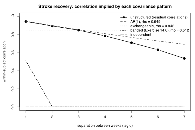
round(emp, 3)
[1] 0.946 0.896 0.850 0.786 0.711 0.632 0.537
(c) What the matrix assumes. Reading the pattern directly: two responses from the same subject are correlated, with correlation \(\rho\), if and only if they are in adjacent weeks; any two measurements two or more weeks apart are assumed uncorrelated. In time series language this is a moving average or one-dependent structure, the covariance analogue of an MA(1) process, and it is the exact opposite of the AR(1) model in Section 14.7, where the correlation \(\rho^{d}\) decays with the separation \(d\) but never reaches zero. It is a strong and, for these data, an implausible assumption: it says that knowing a patient’s ability in week 1 tells you nothing whatever about week 3 once week 2 has been accounted for by the fitted line, and indeed nothing about week 8.
The figure shows how badly that fails. The residual correlations decay slowly and smoothly from \(0.95\) at lag 1 to \(0.54\) at lag 7, closely tracking the AR(1) curve \(0.949^{d}\). The banded model can only fit a spike at lag 1 followed by a flat zero, so it misses six of the seven lags almost entirely, and even at lag 1 the positive definiteness constraint caps it at \(0.53\) against the observed \(0.95\). That is the whole explanation for its DIC: it is a structure designed for short-memory processes being applied to data whose defining feature is a persistent subject-level effect.
The same point can be made from the random effects side. A random intercept model implies exchangeable correlation, constant across all lags; the stroke data sit between that and AR(1). Both are far closer to the truth than a structure that sets the correlation to exactly zero after one week. If a banded structure is ever appropriate for longitudinal data it would be where measurements are far enough apart that dependence genuinely dies out, or where the “correlation” is an artefact of the measurement process (an observer effect spanning consecutive visits, say) rather than a persistent characteristic of the subject.
Backlinks (5)
1. MATH5806 — Applied Regression Analysis at UNSW /blog/pgrad-unsw/math5806/
2. An Introduction to Generalized Linear Models (Dobson & Barnett) /words/library/books/dobson_glm/
Annette J. Dobson and Adrian G. Barnett, An Introduction to Generalized
Linear Models, 4th edition, Chapman & Hall/CRC, 2018. The MATH5806 text:
exponential family, estimation and inference, normal linear models,
binomial and Poisson regression, contingency tables, survival analysis,
clustered and longitudinal data, Bayesian methods and MCMC. The book’s
datasets ship in the dobson R package.
Solutions to every exercise live at Solutions to Dobson & Barnett’s An Introduction to Generalized Linear Models.
3. Estimation & Inference /wiki/ml/supervised/regression/inference/
4. Generalised Linear Models /wiki/ml/supervised/regression/glm/
5. Books /words/library/books/
Here are the books that I have taken the time to create metadata and/or notes for.