Solutions to Cormen, Leiserson, Rivest & Stein’s Introduction to Algorithms
Solutions to every exercise and end-of-chapter problem in Thomas H. Cormen, Charles E. Leiserson, Ronald L. Rivest and Clifford Stein’s Introduction to Algorithms, third edition (MIT Press, 2009): 956 section exercises and 158 problems, appendices included. Every algorithm comes with a correctness proof and a running-time bound, and every algorithm and numeric claim was checked by running it against brute force. The book itself: Introduction to Algorithms.
Chapter 1: The Role of Algorithms in Computing
1.1 Algorithms
Describe a real-world situation that needs sorting, or one that needs the computation of a convex hull.
Sorting: a search engine (or an online shop) must return the matching pages (products) ordered by relevance score (or price), so the \(n\) candidate records must be sorted by key before the first page of results is shown; likewise a bank sorts the day’s cheques by account number before posting them.
Convex hull: to fence the smallest region enclosing a set of \(n\) trees, or to test whether two robots’ footprints can collide, one computes the convex hull of the given points in the plane; the fence posts (or the collision boundary) are exactly the hull’s vertices, and the fence length is the hull’s perimeter.
Apart from running time, which other measures of efficiency might matter in a practical setting?
Memory (space) usage is the main one, alongside several others:
- (i) space: RAM, cache and disk consumed (Section 1.2 names memory as a bounded resource next to time);
- (ii) energy or power draw, decisive on phones, sensors and in data centres;
- (iii) communication: network bandwidth, number of messages, or disk I/O transfers;
- (iv) monetary cost: cloud compute hours, hardware, licences;
- (v) parallel resources: number of processors or machines needed, and how well the work scales across them;
- (vi) latency or worst-case response time (as opposed to throughput), crucial for real-time systems;
- (vii) quality per unit effort: accuracy of an approximate answer, and the programmer time needed to implement and maintain the method.
Pick a data structure you already know and discuss what it does well and where it falls short.
Take the array (a contiguous block of \(n\) equal-sized slots).
Strengths:
- (i) element \(A[i]\) is reached in \(O(1)\) time by address arithmetic (random access);
- (ii) no per-element pointer overhead, and contiguous storage gives excellent cache locality;
- (iii) if kept sorted, membership is answered by binary search in \(O(\lg n)\) time.
Limitations:
- (i) the size is fixed at allocation, so growth requires reallocating and copying (\(\Theta(n)\) per resize, amortized \(O(1)\) per append with geometric, e.g. doubling, growth as in Section 17.4);
- (ii) inserting or deleting at an arbitrary position shifts up to \(n\) elements, costing \(\Theta(n)\);
- (iii) searching an unsorted array takes \(\Theta(n)\), and keeping it sorted makes each insertion \(\Theta(n)\);
- (iv) a large array needs one contiguous chunk of memory, which may be unavailable even when enough total memory is free.
Section 1.1 describes the shortest-path problem (find the shortest route between two intersections of a road map) and the traveling-salesman problem (a truck leaves a depot, visits a set of delivery addresses and returns, and the order of stops should minimize total distance). In what ways are these two problems alike, and in what ways do they differ?
Both are minimum-weight route problems on the same model; they differ in the route’s constraints and, consequently, in their computational difficulty.
Similar:
- (i) both model the road network as a weighted graph (vertices = intersections or addresses, edge weights = distances);
- (ii) both are optimization problems: among exponentially many candidate routes, find one of minimum total length;
- (iii) both have direct applications in transport, logistics and network routing.
Different:
- (i) a shortest path joins two given vertices and may skip every other vertex, while a traveling-salesman tour must visit every delivery address and return to the depot (a Hamiltonian cycle on the addresses, with road distances as weights);
- (ii) shortest paths are solvable efficiently, e.g. by Dijkstra’s algorithm in polynomial time (Chapter 24), whereas the traveling-salesman problem is NP-complete (Section 34.5.4), with no known polynomial-time algorithm;
- (iii) shortest paths have optimal substructure (every subpath of a shortest path is shortest, Lemma 24.1), which the dynamic-programming and greedy methods exploit; for the traveling-salesman problem one instead settles for approximation algorithms (Section 35.2) that guarantee a tour within a constant factor of optimal when the distances obey the triangle inequality.
Give a real-world problem for which nothing short of the best solution is acceptable, and then one for which a solution that is only roughly the best is good enough.
Only the best will do: awarding a scholarship to the highest-scoring applicant; a candidate whose score is merely close to the maximum is the wrong winner, so the exact optimum is required.
Approximately best is fine: the delivery company of Section 1.1 routing its trucks (the traveling-salesman problem); a tour a few percent longer than optimal costs little extra fuel, while finding the true optimum is NP-complete and may be infeasible, so a fast approximation algorithm (Chapter 35) is preferred.
1.2 Algorithms as a technology
Name an application whose purpose, at the level of the application itself, depends on algorithmic content, and describe what the algorithms involved do.
A turn-by-turn navigation service (a phone maps app) is such an application: its core deliverable, the route, is the output of algorithms.
- (i) Shortest paths. The road network is a weighted directed graph (intersections as vertices, road segments as edges weighted by expected travel time). Answering a route query is a single-pair shortest-path problem, solved with Dijkstra’s algorithm (Section 24.3) or a goal-directed variant such as A* with a straight-line-distance heuristic; precomputation schemes speed up the repeated queries on a fixed continental graph.
- (ii) Map matching and geometry. Raw GPS fixes are snapped to the nearest road segment, a nearest-neighbour search over a spatial index, and the displayed map is clipped to the viewport with computational-geometry primitives (Chapter 33).
- (iii) Dynamic re-weighting. Live traffic changes edge weights, so routes are recomputed as data arrive; the algorithms must answer within milliseconds on graphs with tens of millions of vertices, which is only possible because their running times are near-linear rather than exponential.
- (iv) Multi-stop trips. Ordering several delivery stops is a travelling-salesman instance (Section 35.2), NP-complete, so the application uses an approximation or heuristic rather than an exact search.
On one machine, insertion sort takes \(8n^2\) steps on inputs of size \(n\) and merge sort takes \(64n\lg n\) steps. For which \(n\) is insertion sort faster than merge sort?
Insertion sort wins exactly for \(2 \le n \le 43\).
For \(n \ge 1\),
\begin{equation*} 8n^2 < 64 n \lg n \iff n < 8\lg n \iff f(n) := n - 8\lg n < 0 . \end{equation*}
Since \(f^{\prime\prime}(x) = 8/(x^2\ln 2) > 0\), \(f\) is convex on \((0,\infty)\), so \(\{x : f(x) < 0\}\) is an interval. Its integer endpoints are fixed by
\begin{equation*} \begin{aligned} f(1) &= 1 > 0, & f(2) &= 2 - 8 = -6 < 0,\\ f(43) &= 43 - 8\lg 43 \approx -0.41 < 0, & f(44) &= 44 - 8\lg 44 \approx 0.32 > 0, \end{aligned} \end{equation*}
so \(f(n) < 0\) for the integers \(n = 2, 3, \ldots, 43\) and for no others.
Find the least \(n\) for which an algorithm running in time \(100n^2\) is faster than an algorithm running in time \(2^n\) on the same machine.
The smallest such \(n\) is \(n = 15\).
We need \(g(n) := 2^n/n^2 > 100\). For \(n = 1, 2\), \(100n^2 \ge 100 > 4 \ge 2^n\), so the inequality fails. For \(n \ge 3\), \(g\) is increasing, because
\begin{equation*} \frac{g(n+1)}{g(n)} = \frac{2n^2}{(n+1)^2} > 1 \iff \sqrt{2}\,n > n+1 \iff n > \frac{1}{\sqrt 2 - 1} \approx 2.41 . \end{equation*}
Hence for \(3 \le n \le 14\),
\begin{equation*} g(n) \le g(14) = \frac{16384}{196} \approx 83.6 < 100, \end{equation*}
while
\begin{equation*} g(15) = \frac{32768}{225} \approx 145.6 > 100, \end{equation*}
i.e. \(100\cdot 15^2 = 22500 < 32768 = 2^{15}\). By monotonicity the \(100n^2\) algorithm stays faster for every \(n \ge 15\).
Problems for Chapter 1
Comparison of running times: an algorithm takes \(f(n)\) microseconds on an input of size \(n\). For each function \(f(n)\) in the list \(\lg n\), \(\sqrt{n}\), \(n\), \(n\lg n\), \(n^2\), \(n^3\), \(2^n\), \(n!\), and each time budget \(t\) in the list 1 second, 1 minute, 1 hour, 1 day, 1 month, 1 year, 1 century, find the largest problem size \(n\) that can be solved within time \(t\); fill in the resulting table (one row per function, one column per time).
The answer is the largest integer \(n\) with \(f(n) \le T\), where \(T\) is \(t\) in microseconds; taking a month as 30 days, a year as 365 days and a century as 100 years,
\begin{equation*} \begin{aligned} T &= 10^6,\ 6\cdot 10^7,\ 3.6\cdot 10^9,\ 8.64\cdot 10^{10}, \\ &\quad 2.592\cdot 10^{12},\ 3.1536\cdot 10^{13},\ 3.1536\cdot 10^{15}. \end{aligned} \end{equation*}
Since every \(f\) is increasing, the inverses give the entries directly:
\begin{equation*} \begin{aligned} n &= 2^{T},\quad T^2,\quad T, \\ n &= \lfloor T^{1/2}\rfloor,\quad \lfloor T^{1/3}\rfloor,\quad \lfloor \lg T\rfloor \end{aligned} \end{equation*}
for \(\lg n\), \(\sqrt{n}\), \(n\), \(n^2\), \(n^3\), \(2^n\) respectively. For \(n\lg n\) and \(n!\) there is no closed-form inverse; the entry is the \(n\) with \(n\lg n \le T < (n+1)\lg(n+1)\) (found by bisection, as \(n\lg n\) is increasing) and the \(n\) with \(n! \le T < (n+1)!\) (e.g. \(9! = 362880 \le 10^6 < 10! = 3628800\)).
| \(f(n)\) | 1 second | 1 minute | 1 hour | 1 day | 1 month | 1 year | 1 century |
|---|---|---|---|---|---|---|---|
| \(\lg n\) | \(2^{10^6}\) | \(2^{6\cdot 10^7}\) | \(2^{3.6\cdot 10^9}\) | \(2^{8.64\cdot 10^{10}}\) | \(2^{2.592\cdot 10^{12}}\) | \(2^{3.1536\cdot 10^{13}}\) | \(2^{3.1536\cdot 10^{15}}\) |
| \(\sqrt{n}\) | \(10^{12}\) | \(3.6\cdot 10^{15}\) | \(1.296\cdot 10^{19}\) | \(7.46496\cdot 10^{21}\) | \(6.718464\cdot 10^{24}\) | \(9.94519296\cdot 10^{26}\) | \(9.94519296\cdot 10^{30}\) |
| \(n\) | \(10^6\) | \(6\cdot 10^7\) | \(3.6\cdot 10^9\) | \(8.64\cdot 10^{10}\) | \(2.592\cdot 10^{12}\) | \(3.1536\cdot 10^{13}\) | \(3.1536\cdot 10^{15}\) |
| \(n\lg n\) | 62746 | 2801417 | 133378058 | 2755147513 | 71870856404 | 797633893349 | 68610956750570 |
| \(n^2\) | 1000 | 7745 | 60000 | 293938 | 1609968 | 5615692 | 56156922 |
| \(n^3\) | 100 | 391 | 1532 | 4420 | 13736 | 31593 | 146645 |
| \(2^n\) | 19 | 25 | 31 | 36 | 41 | 44 | 51 |
| \(n!\) | 9 | 11 | 12 | 13 | 15 | 16 | 17 |
Chapter 2: Getting Started
2.1 Insertion sort
Following the style of Figure 2.2 (which traces INSERTION-SORT on \(\langle 5,2,4,6,1,3\rangle\), one picture per iteration of the outer for loop), show how INSERTION-SORT operates on the array \(A = \langle 31, 41, 59, 26, 41, 58\rangle\).
The array becomes \(\langle 26, 31, 41, 41, 58, 59\rangle\) after five iterations of the for loop; each row below shows \(A\) at the start of iteration \(j\) (rows (a)-(e)) and the final array (f).
| state | \(j\) | key | \(A[1]\) | \(A[2]\) | \(A[3]\) | \(A[4]\) | \(A[5]\) | \(A[6]\) | values shifted right (line 6) | key placed at (line 8) |
|---|---|---|---|---|---|---|---|---|---|---|
| (a) | 2 | 41 | 31 | 41 | 59 | 26 | 41 | 58 | none | \(A[2]\) |
| (b) | 3 | 59 | 31 | 41 | 59 | 26 | 41 | 58 | none | \(A[3]\) |
| (c) | 4 | 26 | 31 | 41 | 59 | 26 | 41 | 58 | 59, 41, 31 | \(A[1]\) |
| (d) | 5 | 41 | 26 | 31 | 41 | 59 | 41 | 58 | 59 | \(A[4]\) |
| (e) | 6 | 58 | 26 | 31 | 41 | 41 | 59 | 58 | 59 | \(A[5]\) |
| (f) | - | - | 26 | 31 | 41 | 41 | 58 | 59 | - | - |
Modify the INSERTION-SORT procedure so that it sorts the array into nonincreasing order rather than nondecreasing order.
Reverse the comparison on line 5: shift elements right while they are smaller than the key.
NONINCREASING-INSERTION-SORT(A)
1  for j = 2 to A.length
2      key = A[j]
3      // Insert A[j] into the nonincreasing sequence A[1..j-1].
4      i = j - 1
5      while i > 0 and A[i] < key
6          A[i+1] = A[i]
7          i = i - 1
8      A[i+1] = key
Correctness is the Section 2.1 argument with the invariant: at the start of each for-loop iteration, \(A[1\,..\,j-1]\) holds the elements originally in \(A[1\,..\,j-1]\), in nonincreasing order (the while loop stops at the first \(A[i] \ge key\), so placing key at \(A[i+1]\) keeps \(A[1\,..\,j]\) nonincreasing).
The searching problem takes as input a sequence of \(n\) numbers \(A = \langle a_1, a_2, \ldots, a_n\rangle\) together with a value \(v\), and must output an index \(i\) with \(v = A[i]\), or the special value NIL when \(v\) does not occur in \(A\). Give pseudocode for linear search, which examines the sequence element by element looking for \(v\). Prove the algorithm correct with a loop invariant, checking that the invariant satisfies all three required properties (initialization, maintenance, termination).
Scan \(A[1], A[2], \ldots\) in order and return the first index holding \(v\); return NIL if the scan finishes.
LINEAR-SEARCH(A, v)
1  for i = 1 to A.length
2      if A[i] == v
3          return i
4  return NIL
Loop invariant: at the start of each iteration of the for loop of lines 1-3, \(v \notin A[1\,..\,i-1]\).
Initialization: before the first iteration \(i = 1\), and \(A[1\,..\,0]\) is empty, so it does not contain \(v\).
Maintenance: suppose the invariant holds at the start of the iteration for \(i\). If \(A[i] = v\), line 3 returns \(i\), which is a correct answer. Otherwise \(A[i] \ne v\), and together with \(v \notin A[1\,..\,i-1]\) this gives \(v \notin A[1\,..\,i]\), which is the invariant for the next value \(i+1\).
Termination: the procedure either returns at line 3 an index \(i\) with \(A[i] = v\) (correct), or the loop exits because \(i = A.length + 1 = n+1\); then the invariant says \(v \notin A[1\,..\,n]\), so \(v\) does not appear in \(A\) and returning NIL on line 4 is correct.
Two \(n\)-bit binary integers are held in two arrays \(A\) and \(B\), each with \(n\) elements. Their sum is to be written in binary into an array \(C\) with \(n+1\) elements. Give a formal statement of this problem, and write pseudocode that adds the two integers.
Formally (storing the least significant bit first):
Input: two arrays \(A[1\,..\,n]\) and \(B[1\,..\,n]\) with every entry in \(\{0,1\}\), representing \(a = \sum_{k=1}^{n} A[k]\,2^{k-1}\) and \(b = \sum_{k=1}^{n} B[k]\,2^{k-1}\).
Output: an array \(C[1\,..\,n+1]\) with every entry in \(\{0,1\}\) such that \(\sum_{k=1}^{n+1} C[k]\,2^{k-1} = a + b\).
The algorithm is grade-school addition with a carry bit, from the low-order end.
BINARY-ADD(A, B, n)
1  let C[1..n+1] be a new array
2  carry = 0
3  for i = 1 to n
4      s = A[i] + B[i] + carry
5      C[i] = s mod 2
6      carry = floor(s / 2)
7  C[n+1] = carry
8  return C
Loop invariant: at the start of each iteration of the for loop, \(carry \in \{0,1\}\) and
\begin{equation*} \begin{aligned} \sum_{k=1}^{i-1} C[k]\,2^{k-1} + carry \cdot 2^{i-1} &= \sum_{k=1}^{i-1} (A[k]+B[k])\,2^{k-1}. \end{aligned} \end{equation*}
Initialization: \(i = 1\) and \(carry = 0\), so both sides are \(0\). Maintenance: \(s = A[i] + B[i] + carry \in \{0,1,2,3\}\) and \(s = C[i] + 2\,carry^{\prime}\) with \(C[i], carry^{\prime} \in \{0,1\}\) after lines 5-6, so
\begin{equation*} \begin{aligned} \sum_{k=1}^{i} C[k]\,2^{k-1} + carry^{\prime} \cdot 2^{i} &= \sum_{k=1}^{i-1} C[k]\,2^{k-1} + (C[i] + 2\,carry^{\prime})\,2^{i-1} \\ &= \sum_{k=1}^{i-1} C[k]\,2^{k-1} + carry \cdot 2^{i-1} + (A[i]+B[i])\,2^{i-1} \\ &= \sum_{k=1}^{i} (A[k]+B[k])\,2^{k-1}, \end{aligned} \end{equation*}
which is the invariant for \(i+1\). Termination: the loop exits with \(i = n+1\), and line 7 sets \(C[n+1] = carry\), so the invariant becomes \(\sum_{k=1}^{n+1} C[k]\,2^{k-1} = a + b\), with every \(C[k] \in \{0,1\}\).
2.2 Analyzing algorithms
Write the function \(n^3/1000 - 100n^2 - 100n + 3\) in \(\Theta\)-notation.
\(f(n) = n^3/1000 - 100n^2 - 100n + 3 = \Theta(n^3)\). For \(n \ge 1\) we have \(-100n^2 - 100n + 3 < 0\), and for \(n \ge 400000\) we have \(n^3/2000 \ge 200n^2 \ge 100n^2 + 100n\), so
\begin{equation*} \begin{aligned} f(n) &\le \frac{n^3}{1000} && (n \ge 1),\\ f(n) &\ge \frac{n^3}{1000} - \frac{n^3}{2000} = \frac{n^3}{2000} && (n \ge 400000). \end{aligned} \end{equation*}
Hence \(c_1 n^3 \le f(n) \le c_2 n^3\) for all \(n \ge n_0\) with \(c_1 = 1/2000\), \(c_2 = 1/1000\), \(n_0 = 400000\), and so \(f(n) = \Theta(n^3)\).
To sort \(n\) numbers in an array \(A\), find the smallest element of \(A\) and swap it with \(A[1]\); then find the second smallest element and swap it with \(A[2]\); keep going in this way for the first \(n-1\) positions of \(A\). Give pseudocode for this algorithm, called selection sort. Which loop invariant does it maintain? Why is it enough to run it over only the first \(n-1\) elements instead of all \(n\)? Give its best-case and worst-case running times in \(\Theta\)-notation.
Selection sort runs in \(\Theta(n^2)\) time in both the best and the worst case. Here is the pseudocode:
SELECTION-SORT(A)
1  n = A.length
2  for i = 1 to n - 1
3      smallest = i
4      for j = i + 1 to n
5          if A[j] < A[smallest]
6              smallest = j
7      exchange A[i] with A[smallest]
Loop invariant: at the start of each iteration of the for loop of lines 2–7, the subarray \(A[1..i-1]\) holds the \(i-1\) smallest elements of \(A\) in sorted order, and \(A[i..n]\) holds the remaining elements.
Initialization: for \(i = 1\) the subarray \(A[1..0]\) is empty.
Maintenance: lines 3–6 leave \(smallest\) as the index of a minimum of \(A[i..n]\) (this is the inner loop’s own invariant: \(A[smallest] = \min A[i..j-1]\)). By the invariant, that minimum is at least every element of \(A[1..i-1]\) and is an \(i\)-th smallest element of \(A\). Line 7 puts it in \(A[i]\), so \(A[1..i]\) holds the \(i\) smallest elements in sorted order. Incrementing \(i\) restores the invariant.
Termination: the loop stops when \(i = n\). Then \(A[1..n-1]\) holds the \(n-1\) smallest elements in sorted order, so \(A[n]\) is a largest element and the whole of \(A[1..n]\) is sorted.
That last step is why only \(n-1\) passes are needed. Once the \(n-1\) smallest elements are in place, the one element left over is forced to be the largest, and it already sits in \(A[n]\). A pass with \(i = n\) would compare nothing and swap \(A[n]\) with itself.
Running time: the inner loop body (lines 5–6) runs \(n - i\) times on pass \(i\) for every input, because the loop bounds do not depend on the data. Only the assignment in line 6 depends on the input, and it costs at most a constant per test. So the total time is
\begin{equation*} \Theta\Bigl(n + \sum_{i=1}^{n-1} (n-i)\Bigr) = \Theta\Bigl(n + \frac{n(n-1)}{2}\Bigr) = \Theta(n^2) \end{equation*}
for every input, so the best and worst cases are both \(\Theta(n^2)\).
Go back to linear search (Exercise 2.1-3), which scans \(A[1..n]\) for a value \(v\). Suppose the element being searched for is equally likely to be any element of the array. On average, how many elements of the input have to be checked? How many in the worst case? Give the average-case and worst-case running times of linear search in \(\Theta\)-notation, with justification.
On average \((n+1)/2\) elements are checked, in the worst case \(n\), and both running times are \(\Theta(n)\). Assume the target is the element in position \(k\), where \(k\) is uniform on \(\{1,\dots,n\}\) and the elements are distinct (if there are repeats, take \(k\) to be the position of the first occurrence). Then the search checks exactly \(A[1],\dots,A[k]\), which is \(k\) elements, so the expected number checked is
\begin{equation*} \mathrm{E}[k] = \frac{1}{n}\sum_{k=1}^{n} k = \frac{1}{n}\cdot\frac{n(n+1)}{2} = \frac{n+1}{2}. \end{equation*}
In the worst case all \(n\) elements are checked: this happens when \(v = A[n]\) only, or when \(v\) is not in the array at all.
Each check costs a constant amount of time (a loop test, a comparison and an increment), and there is a constant amount of overhead outside the loop. So the running time on an input that checks \(k\) elements is \(a k + b\) for constants \(a > 0\) and \(b\). The average-case time is therefore
\begin{equation*} a\cdot\frac{n+1}{2} + b = \Theta(n), \end{equation*}
and the worst-case time is \(a n + b = \Theta(n)\).
What modification gives almost any algorithm a good best-case running time?
Add a special case at the start. The algorithm first checks whether the input is one particular input (or belongs to a class of inputs) whose answer is precomputed or cheap to get. If it is, the algorithm returns that answer right away; if not, it runs the original algorithm.
For example, a sorting algorithm can first scan \(A\) in \(\Theta(n)\) time to test whether \(A\) is already sorted, and return immediately if so. Its best-case running time drops to \(\Theta(n)\). The scan adds only \(O(n)\) to every other input, so the worst case does not change asymptotically.
2.3 Designing algorithms
Following the style of Figure 2.4 (which shows merge sort on \(\langle 5,2,4,7,1,3,2,6 \rangle\) bottom-up, as successive rounds of merging sorted runs), show how merge sort operates on the array \(A = \langle 3, 41, 52, 26, 38, 57, 9, 49 \rangle\).
Reading bottom-up as in Figure 2.4, the eight singletons are merged in pairs, then the pairs into runs of four, then the two runs into the sorted output:
| stage | sorted runs |
|---|---|
| initial sequence | \(\langle 3\rangle\) \(\langle 41\rangle\) \(\langle 52\rangle\) \(\langle 26\rangle\) \(\langle 38\rangle\) \(\langle 57\rangle\) \(\langle 9\rangle\) \(\langle 49\rangle\) |
| after merging pairs | \(\langle 3,41\rangle\) \(\langle 26,52\rangle\) \(\langle 38,57\rangle\) \(\langle 9,49\rangle\) |
| after merging fours | \(\langle 3,26,41,52\rangle\) \(\langle 9,38,49,57\rangle\) |
| sorted sequence | \(\langle 3,9,26,38,41,49,52,57\rangle\) |
Each run in a row is the MERGE of two adjacent runs in the row above it.
Rewrite MERGE so that it uses no sentinels: it should stop comparing as soon as one of the arrays \(L\), \(R\) has had all of its elements copied back into \(A\), and then copy whatever remains of the other array into \(A\).
Compare heads only while both arrays are nonempty, then drain the leftover array:
MERGE(A, p, q, r)
 1  n1 = q - p + 1
 2  n2 = r - q
 3  let L[1..n1] and R[1..n2] be new arrays
 4  for i = 1 to n1
 5      L[i] = A[p + i - 1]
 6  for j = 1 to n2
 7      R[j] = A[q + j]
 8  i = 1
 9  j = 1
10  k = p
11  while i <= n1 and j <= n2
12      if L[i] <= R[j]
13          A[k] = L[i];  i = i + 1
14      else A[k] = R[j];  j = j + 1
15      k = k + 1
16  while i <= n1
17      A[k] = L[i];  i = i + 1;  k = k + 1
18  while j <= n2
19      A[k] = R[j];  j = j + 1;  k = k + 1
While both \(i \le n_1\) and \(j \le n_2\), line 12 makes exactly the comparison of the sentinel version, so the loop invariant of Section 2.3.1 holds through lines 11–15. When one array, say \(R\), is exhausted, the uncopied \(L[i \mathbin{..} n_1]\) is sorted and, by the invariant, no smaller than anything in \(A[p \mathbin{..} k-1]\); lines 16–17 append it, and line 18 does nothing (symmetrically if \(L\) is exhausted). Each loop iteration copies one element, so the running time is still \(\Theta(n)\) with \(n = r-p+1\).
Prove by mathematical induction that, for \(n\) an exact power of \(2\), the recurrence
\begin{equation*} T(n) = \begin{cases} 2 & \text{if } n = 2, \\ 2T(n/2) + n & \text{if } n = 2^k \text{ for some } k > 1 \end{cases} \end{equation*}
has solution \(T(n) = n \lg n\).
Induct on \(k \ge 1\), where \(n = 2^k\). Base case \(k=1\): \(T(2) = 2 = 2\lg 2\). Inductive step: for \(k > 1\) assume \(T(2^{k-1}) = 2^{k-1}(k-1)\), i.e. \(T(n/2) = (n/2)\lg(n/2)\). Then
\begin{equation*} \begin{aligned} T(n) &= 2T(n/2) + n = 2 \cdot \frac{n}{2}\lg\frac{n}{2} + n \\ &= n(\lg n - 1) + n = n \lg n . \end{aligned} \end{equation*}
Hence \(T(n) = n\lg n\) for every \(n = 2^k\), \(k \ge 1\).
Insertion sort can be phrased recursively: to sort \(A[1 \mathbin{..} n]\), first sort \(A[1 \mathbin{..} n-1]\) recursively, then insert \(A[n]\) into the now-sorted \(A[1 \mathbin{..} n-1]\). Give a recurrence for the worst-case running time of this recursive version.
\begin{equation*} T(n) = \begin{cases} \Theta(1) & \text{if } n = 1, \\ T(n-1) + \Theta(n) & \text{if } n > 1. \end{cases} \end{equation*}
The recursive call costs \(T(n-1)\) in the worst case, and inserting \(A[n]\) into the sorted \(A[1 \mathbin{..} n-1]\) is one pass of the while loop of lines 5–7 of INSERTION-SORT, which shifts up to \(n-1\) elements, so it costs \(O(n)\), and \(\Theta(n)\) when \(A[n]\) is smaller than all of \(A[1 \mathbin{..} n-1]\). Both worst cases occur together on a reverse-sorted input: its prefix \(A[1 \mathbin{..} n-1]\) is itself reverse sorted, and \(A[n]\) is its minimum.
Recall the searching problem of Exercise 2.1-3: given a sequence \(A = \langle a_1, \dots, a_n\rangle\) and a value \(v\), return an index \(i\) with \(v = A[i]\), or NIL if \(v\) does not occur in \(A\). When \(A\) is sorted, comparing \(v\) with the middle element lets us discard half of the sequence; binary search repeats this, halving the remaining portion each time. Give pseudocode (iterative or recursive) for binary search, and argue that its worst-case running time is \(\Theta(\lg n)\).
Keep a window \(A[low \mathbin{..} high]\) that must contain \(v\) if \(v\) occurs at all, and halve it by probing its midpoint:
BINARY-SEARCH(A, v)
 1  low = 1
 2  high = A.length
 3  while low <= high
 4      mid = floor((low + high) / 2)
 5      if A[mid] == v
 6          return mid
 7      elseif A[mid] < v
 8          low = mid + 1
 9      else high = mid - 1
10  return NIL
Correctness. Loop invariant: at the start of each iteration, if \(v\) occurs in \(A\) then it occurs in \(A[low \mathbin{..} high]\). Initialization: the window is all of \(A\). Maintenance: if \(A[mid] < v\) then, \(A\) being sorted, \(A[low \mathbin{..} mid] < v\), so \(v\) can only lie in \(A[mid+1 \mathbin{..} high]\); symmetrically if \(A[mid] > v\). Termination: a return in line 6 is correct since \(A[mid] = v\); otherwise the loop exits with \(low > high\), the window is empty, and by the invariant \(v \notin A\), so NIL is correct.
Running time. Each iteration costs \(\Theta(1)\). Let \(m = high - low + 1\) be the window size. Since \(mid - low = \lfloor (m-1)/2 \rfloor\) and \(high - mid = \lceil (m-1)/2 \rceil\), an iteration that does not return leaves a window of size at most \(\lceil (m-1)/2 \rceil = \lfloor m/2 \rfloor\). By induction, after \(t\) iterations the size is at most \(\lfloor n/2^t \rfloor\), which is \(0\) once \(t = \lfloor \lg n \rfloor + 1\); so there are at most \(\lfloor \lg n \rfloor + 1\) iterations and the running time is \(O(\lg n)\). Conversely, if \(v\) exceeds every element, line 8 runs every time and the size goes from \(m\) to exactly \(\lfloor m/2 \rfloor\), so exactly \(\lfloor \lg n \rfloor + 1\) iterations are executed. Hence the worst case is \(\Theta(\lg n)\).
The while loop in lines 5–7 of INSERTION-SORT (Section 2.1) finds where to put the key by scanning the sorted prefix \(A[1 \mathbin{..} j-1]\) linearly from right to left. If we replace this linear scan with a binary search (Exercise 2.3-5), does the worst-case running time of insertion sort drop to \(\Theta(n \lg n)\)?
No: binary search finds the insertion point with \(O(\lg j)\) comparisons, but inserting the key still requires shifting every element of \(A[1 \mathbin{..} j-1]\) larger than it one place to the right, and that is \(j-1\) moves in the worst case. On a reverse-sorted input every key \(A[j]\) is smaller than all of \(A[1 \mathbin{..} j-1]\), so iteration \(j\) performs \(j-1\) shifts regardless of how the position was found, and the total work is at least
\begin{equation*} \sum_{j=2}^{n} (j-1) = \frac{n(n-1)}{2} = \Theta(n^2). \end{equation*}
Each iteration still costs \(O(j)\), so the worst case stays \(\Theta(n^2)\).
Given a set \(S\) of \(n\) integers and a further integer \(x\), describe an algorithm running in \(\Theta(n \lg n)\) time that decides whether \(S\) contains two elements whose sum equals \(x\) exactly.
Sort \(S\) with merge sort, then sweep two indices inward from the ends of the sorted array: if the current pair sums to less than \(x\), advance the left index; if more, retreat the right index; stop on equality or when the indices meet.
SUM-EXISTS(S, x)
1  let A[1..n] hold the elements of S
2  MERGE-SORT(A, 1, n)
3  i = 1
4  j = n
5  while i < j
6      if A[i] + A[j] == x
7          return TRUE
8      elseif A[i] + A[j] < x
9          i = i + 1
10     else j = j - 1
11 return FALSE
Correctness rests on the loop invariant: at the start of each iteration of lines 5–10, every pair of indices \(p < q\) with \(A[p] + A[q] = x\) satisfies \(i \le p < q \le j\).
Initialization: \(i = 1\) and \(j = n\), so every pair \(p < q\) lies in \([i, j]\).
Maintenance: if line 7 is not reached, suppose \(A[i] + A[j] < x\). Since \(A\) is sorted, for every \(q\) with \(i < q \le j\),
\begin{equation*} A[i] + A[q] \le A[i] + A[j] < x, \end{equation*}
so no solution pair has \(p = i\), and incrementing \(i\) preserves the invariant. Symmetrically, if \(A[i] + A[j] > x\) then \(A[p] + A[j] \ge A[i] + A[j] > x\) for all \(i \le p < j\), so no solution pair has \(q = j\), and decrementing \(j\) preserves it.
Termination: a TRUE return at line 7 exhibits the pair \(A[i], A[j]\) with \(i < j\). Otherwise the loop ends with \(i \ge j\), so no indices \(p < q\) satisfy \(i \le p < q \le j\); by the invariant there is no solution pair, and FALSE is correct.
Running time: line 2 costs \(\Theta(n \lg n)\) (Section 2.3.2). Each iteration of the loop decreases \(j - i\) by \(1\), and \(j - i = n - 1\) at the start, so there are at most \(n - 1\) iterations of \(O(1)\) work each. The total is \(\Theta(n \lg n) + O(n) = \Theta(n \lg n)\).
Problems for Chapter 2
Insertion sort on small arrays in merge sort: merge sort takes \(\Theta(n\lg n)\) worst-case time and insertion sort \(\Theta(n^2)\), yet insertion sort’s small constant factors can make it the faster of the two on small inputs, so it is sensible to “coarsen” the leaves of merge sort’s recursion by switching to insertion sort once subproblems are small enough. Consider the variant of merge sort that sorts \(n/k\) sublists, each of length \(k\), by insertion sort, and then merges them with the usual merging procedure; the parameter \(k\) is to be chosen.
(a) Show that insertion sort sorts the \(n/k\) sublists of length \(k\) in \(\Theta(nk)\) worst-case time.
(b) Show how to merge the sublists in \(\Theta(n\lg(n/k))\) worst-case time.
(c) Granting that the modified algorithm runs in \(\Theta(nk+n\lg(n/k))\) worst-case time, what is the largest \(k\), as a function of \(n\) and in \(\Theta\)-notation, for which the modified algorithm has the same running time as standard merge sort?
(d) How should \(k\) be chosen in practice?
(a) By Section 2.2, insertion sort on \(k\) elements takes worst-case time \(ak^2+bk+c=\Theta(k^2)\), so there are constants \(0<c_1\le c_2\) with \(c_1k^2\le T_{\mathrm{ins}}(k)\le c_2k^2\) for all \(k\ge 1\). Hence the \(n/k\) sublists cost
\begin{equation*} \frac{n}{k}\,T_{\mathrm{ins}}(k)\in\Big[\frac{n}{k}c_1k^2,\ \frac{n}{k}c_2k^2\Big]=[c_1nk,\ c_2nk], \end{equation*}
which is \(\Theta(nk)\), the upper bound being attained when every sublist is reverse sorted.
(b) Run merge sort but stop the recursion at subarrays of length \(k\) (assume, as in Section 2.3.2, that \(n/k\) is a power of \(2\)):
COARSE-MERGE-SORT(A, p, r, k)
1  if r - p + 1 <= k
2      INSERTION-SORT(A, p, r)      // sort A[p..r] in place
3  else q = floor((p + r)/2)
4      COARSE-MERGE-SORT(A, p, q, k)
5      COARSE-MERGE-SORT(A, q + 1, r, k)
6      MERGE(A, p, q, r)
Correctness is that of MERGE-SORT (Section 2.3.1), with sorted leaves supplied by insertion sort. For the cost of the merging, use the recursion tree of Figure 2.5 truncated where subproblems reach size \(k\): level \(d\) has \(2^d\) subarrays of size \(n/2^d\), and MERGE on a subarray of length \(m\) takes \(\Theta(m)\) time (it copies all \(m\) elements and does \(m\) iterations of lines 12–17), so every level costs \(\Theta(n)\). The leaves sit at depth \(\lg(n/k)\), so there are \(\lg(n/k)\) levels of merging and
\begin{equation*} T_{\mathrm{merge}}(n)=\lg(n/k)\cdot\Theta(n)=\Theta\big(n\lg(n/k)\big). \end{equation*}
(c) The largest such \(k\) is \(k=\Theta(\lg n)\). If \(k=O(\lg n)\), then, using \(\lg k\le k\),
\begin{equation*} \begin{aligned} nk+n\lg(n/k)&\le O(n\lg n)+n\lg n=O(n\lg n),\\ nk+n\lg(n/k)&=n\lg n+n(k-\lg k)\ge n\lg n, \end{aligned} \end{equation*}
so the running time is \(\Theta(n\lg n)\), the same as merge sort. If \(k\) is not \(O(\lg n)\), then \(nk\) is not \(O(n\lg n)\) and the modified algorithm is asymptotically slower. So \(k=\Theta(\lg n)\) is the largest admissible order of growth.
(d) Choose \(k\) as the largest sublist length on which insertion sort is still faster than merge sort on the actual machine, i.e. the crossover point where \(c_{\mathrm{ins}}k^2\) overtakes \(c_{\mathrm{merge}}k\lg k\); it is found by timing both sorts on inputs of increasing size, and is a small constant (typically tens of elements).
Correctness of bubblesort: bubblesort is a well-known but inefficient sorting algorithm that keeps exchanging adjacent elements that are out of order:
BUBBLESORT(A)
1  for i = 1 to A.length - 1
2      for j = A.length downto i + 1
3          if A[j] < A[j - 1]
4              exchange A[j] with A[j - 1]
(a) Let \(A^{\prime}\) be the output of BUBBLESORT\((A)\) and \(n=A.\mathit{length}\). Proving correctness requires showing that the procedure terminates and that
\begin{equation*} A^{\prime}[1]\le A^{\prime}[2]\le\cdots\le A^{\prime}[n]. \qquad (2.3) \end{equation*}
What else must be proved to show that BUBBLESORT really sorts?
Parts (b) and (c) prove inequality (2.3).
(b) State a precise loop invariant for the for loop of lines 2–4 and prove that it holds, following the structure of the loop-invariant proofs in this chapter.
(c) Using the termination condition of the invariant from (b), state a loop invariant for the for loop of lines 1–4 that yields inequality (2.3), and prove it with the same structure.
(d) What is the worst-case running time of bubblesort, and how does it compare with that of insertion sort?
(a) We must also prove that \(A^{\prime}\) is a permutation of the input \(A\), i.e. that \(A^{\prime}\) consists of exactly the original elements. (Here this is immediate: the array is modified only by the exchanges of line 4, and each exchange permutes its entries.)
(b) Invariant: at the start of each iteration of the for loop of lines 2–4, the subarray \(A[j\,..\,n]\) consists of the elements originally in \(A[j\,..\,n]\) before the inner loop began, possibly reordered, \(A[1\,..\,j-1]\) is unchanged, and \(A[j]\) is the smallest element of \(A[j\,..\,n]\).
Initialization: before the first iteration \(j=n\); nothing has moved, and \(A[n\,..\,n]\) has the single element \(A[n]\), which is its own minimum.
Maintenance: by the invariant \(A[j]=\min A[j\,..\,n]\). Lines 3–4 exchange \(A[j]\) and \(A[j-1]\) exactly when \(A[j]<A[j-1]\), so afterwards
\begin{equation*} A[j-1]=\min(A[j-1],A[j])=\min A[j-1\,..\,n], \end{equation*}
and the only change was a swap inside \(A[j-1\,..\,n]\), leaving \(A[1\,..\,j-2]\) unchanged. Decrementing \(j\) re-establishes the invariant.
Termination: the loop ends when \(j=i\). Then \(A[i\,..\,n]\) is a permutation of its contents before the inner loop, \(A[1\,..\,i-1]\) is unchanged, and \(A[i]\) is the smallest element of \(A[i\,..\,n]\).
(c) Invariant: at the start of each iteration of the for loop of lines 1–4, \(A\) is a permutation of the input, \(A[1\,..\,i-1]\) is sorted, and every element of \(A[1\,..\,i-1]\) is \(\le\) every element of \(A[i\,..\,n]\).
Initialization: \(i=1\), so \(A[1\,..\,0]\) is empty and the claims hold vacuously.
Maintenance: by the termination condition of (b), the inner loop leaves \(A[1\,..\,i-1]\) alone, permutes \(A[i\,..\,n]\), and puts \(A[i]=\min A[i\,..\,n]\). Since the permuted block has the same elements, every element of \(A[1\,..\,i-1]\) is still \(\le\) every element of \(A[i\,..\,n]\); in particular \(A[i-1]\le A[i]\), so \(A[1\,..\,i]\) is sorted, and \(A[i]\le A[i+1\,..\,n]\) by minimality. Incrementing \(i\) re-establishes the invariant.
Termination: the loop ends at \(i=n\). Then \(A[1\,..\,n-1]\) is sorted and each of its elements is \(\le A[n]\), so
\begin{equation*} A[1]\le A[2]\le\cdots\le A[n-1]\le A[n], \end{equation*}
which is (2.3); with the permutation clause this proves that BUBBLESORT sorts.
(d) Bubblesort runs in \(\Theta(n^2)\) time in the worst case, and in fact on every input. Each test in line 3 costs \(\Theta(1)\), and that test is executed
\begin{equation*} \sum_{i=1}^{n-1}(n-i)=\frac{n(n-1)}{2} \end{equation*}
times whatever the input, while the loop overhead and line 4 cost at most a constant factor more. Insertion sort has the same \(\Theta(n^2)\) worst case (Section 2.2), but its best case is \(\Theta(n)\) (already sorted input), whereas bubblesort never does better than \(\Theta(n^2)\); on every input bubblesort makes at least as many comparisons as insertion sort, so in practice it is the slower of the two.
Correctness of Horner’s rule: Horner’s rule evaluates the polynomial
\begin{equation*} \begin{aligned} P(x) &= \sum_{k=0}^{n} a_k x^k \\ &= a_0 + x(a_1 + x(a_2 + \cdots + x(a_{n-1} + x a_n)\cdots)), \end{aligned} \end{equation*}
from the coefficients \(a_0, a_1, \ldots, a_n\) and a value of \(x\), via the fragment
1  y = 0
2  for i = n downto 0
3      y = a_i + x * y
(a) What is the running time of this fragment, in \(\Theta\)-notation?
(b) Give pseudocode for the naive evaluation algorithm, which computes every term of the polynomial from scratch. What is its running time, and how does it compare with Horner’s rule?
(c) Take as loop invariant: at the start of each iteration of the for loop of lines 2–3,
\begin{equation*} y = \sum_{k=0}^{n-(i+1)} a_{k+i+1} x^k , \end{equation*}
where an empty sum counts as \(0\). Following the structure of the chapter’s loop-invariant proofs, use it to show that \(y = \sum_{k=0}^{n} a_k x^k\) when the loop terminates.
(d) Conclude that the fragment correctly evaluates the polynomial with coefficients \(a_0, a_1, \ldots, a_n\).
(a) \(\Theta(n)\): the loop body runs \(n+1\) times (for \(i = n, n-1, \ldots, 0\)), each time doing one multiplication, one addition and one assignment in constant time, and the loop test runs \(n+2\) times.
(b) The naive algorithm takes \(\Theta(n^2)\) time, a factor of \(n\) slower than Horner’s rule.
NAIVE-POLY-EVAL(a, n, x)
1  y = 0
2  for k = 0 to n
3      t = 1
4      for j = 1 to k
5          t = t * x
6      y = y + a_k * t
7  return y
For each \(k\) the inner loop of lines 4–5 performs \(k\) multiplications, so the total work is
\begin{equation*} \sum_{k=0}^{n} \Theta(k + 1) = \Theta\!\left(\frac{(n+1)(n+2)}{2}\right) = \Theta(n^2). \end{equation*}
Horner’s rule needs only \(n+1\) multiplications in total.
(c) Initialization: before the first iteration \(i = n\), so the sum runs from \(k = 0\) to \(-1\), is empty, and equals \(0 = y\).
Maintenance: suppose the invariant holds at the start of the iteration with index \(i\). Line 3 sets
\begin{equation*} \begin{aligned} y^{\prime} = a_i + x y &= a_i + \sum_{k=0}^{n-i-1} a_{k+i+1} x^{k+1} \\ &= a_i + \sum_{k=1}^{n-i} a_{k+i} x^{k} = \sum_{k=0}^{n-i} a_{k+i} x^{k}, \end{aligned} \end{equation*}
and the next iteration has index \(i^{\prime} = i - 1\), for which \(n - (i^{\prime}+1) = n - i\) and \(a_{k+i^{\prime}+1} = a_{k+i}\). So the invariant holds at the start of the next iteration.
Termination: the loop ends when \(i = -1\). Substituting \(i = -1\) into the invariant gives
\begin{equation*} y = \sum_{k=0}^{n} a_{k} x^k . \end{equation*}
(d) The loop runs exactly \(n+1\) iterations and so terminates, and by (c) the final value of \(y\) is \(\sum_{k=0}^{n} a_k x^k = P(x)\). Hence the fragment correctly evaluates the polynomial with coefficients \(a_0, a_1, \ldots, a_n\) at \(x\).
Inversions: let \(A[1 \ldots n]\) be an array of \(n\) distinct numbers. A pair \((i, j)\) with \(i < j\) and \(A[i] > A[j]\) is called an inversion of \(A\).
(a) List the five inversions of the array \(\langle 2, 3, 8, 6, 1 \rangle\).
(b) Which array with elements drawn from \(\{1, 2, \ldots, n\}\) has the largest number of inversions, and how many does it have?
(c) How is the running time of insertion sort related to the number of inversions in its input array? Justify the answer.
(d) Give an algorithm that counts the inversions of any permutation of \(n\) elements in \(\Theta(n \lg n)\) worst-case time. (Hint: modify merge sort.)
(a) The inversions are \((1,5), (2,5), (3,4), (3,5), (4,5)\), i.e. the value pairs \(2 > 1\), \(3 > 1\), \(8 > 6\), \(8 > 1\), \(6 > 1\).
(b) The reversed array \(\langle n, n-1, \ldots, 1 \rangle\), with \(\binom{n}{2} = n(n-1)/2\) inversions. Any array has at most \(\binom{n}{2}\) pairs \(i < j\), and in the reversed array \(A[i] = n + 1 - i > n + 1 - j = A[j]\) for every such pair, so all of them are inversions. It is the unique maximizer: if every pair is inverted, \(A\) is strictly decreasing, hence the reversed array.
(c) Insertion sort runs in \(\Theta(n + I)\) time on an input with \(I\) inversions: the while loop of lines 5–7 of INSERTION-SORT (Section 2.1) executes its body exactly \(I\) times in total.
Fix an iteration \(j\) of the outer loop with key \(= A[j]\) (original position \(j\)). By the loop invariant of Section 2.1, \(A[1 \ldots j-1]\) then holds the original elements of positions \(1, \ldots, j-1\) in sorted order. The while loop shifts right exactly those of them that exceed the key, and stops at the first one that does not. So the number of shifts in iteration \(j\) is
\begin{equation*} \#\{\, i < j : A[i] > A[j] \,\} , \end{equation*}
the number of inversions whose second index is \(j\). Summing over \(j = 2, \ldots, n\) counts every inversion once, giving \(I\) shifts in total. Each outer iteration costs \(\Theta(1)\) besides its shifts, and each shift costs \(\Theta(1)\), so the running time is \(\Theta(n) + \Theta(I) = \Theta(n + I)\).
(d) Run merge sort, and in each merge add the number of cross inversions: whenever an element of the right half is copied out, every element still waiting in the left half is larger than it and forms an inversion with it.
COUNT-INVERSIONS(A, p, r)
1  if p >= r
2      return 0
3  q = floor((p + r) / 2)
4  c = COUNT-INVERSIONS(A, p, q) + COUNT-INVERSIONS(A, q + 1, r)
5  return c + MERGE-INVERSIONS(A, p, q, r)

MERGE-INVERSIONS(A, p, q, r)
1  n1 = q - p + 1
2  copy A[p..q] into L[1..n1] and A[q+1..r] into R[1..r-q]
3  L[n1 + 1] = infinity, R[r - q + 1] = infinity
4  i = 1, j = 1, c = 0
5  for k = p to r
6      if L[i] <= R[j]
7          A[k] = L[i], i = i + 1
8      else A[k] = R[j], j = j + 1
9          c = c + n1 - i + 1
10 return c
Correctness, by induction on \(r - p\): COUNT-INVERSIONS\((A, p, r)\) returns the number of inversions of \(A[p \ldots r]\) and leaves it sorted. A subarray of length at most \(1\) has no inversions. Otherwise, each inversion \((s, t)\) of \(A[p \ldots r]\) has either \(s < t \le q\), or \(q < s < t\), or \(s \le q < t\); by the inductive hypothesis line 4 counts the first two kinds and sorts both halves. The number of cross pairs, i.e. pairs \((x, y)\) with \(x\) in the left half, \(y\) in the right half and \(x > y\), depends only on the sets of elements in the two halves, so sorting them does not change it. MERGE-INVERSIONS is MERGE (Section 2.3.1) with line 9 added, so it produces the sorted output. When an element \(y = R[j]\) is copied at line 8, the elements copied before it are smaller and those copied after it are larger (distinct elements, sorted output). Hence the left-half elements larger than \(y\) are exactly the not-yet-copied \(L[i \ldots n_1]\), which number \(n_1 - i + 1\) (the sentinel is never counted, as \(i \le n_1 + 1\)). Summing over all \(y\), line 9 accumulates exactly the cross inversions, which completes the induction.
Running time: MERGE-INVERSIONS does \(\Theta(1)\) extra work per iteration on top of MERGE, so it runs in \(\Theta(n)\) time, and the running time satisfies the merge-sort recurrence \(T(n) = 2T(n/2) + \Theta(n)\), whose solution is \(\Theta(n \lg n)\) (Section 2.3.2).
Chapter 3: Growth of Functions
3.1 Asymptotic notation
Suppose \(f(n)\) and \(g(n)\) are asymptotically nonnegative. Working directly from the definition of \(\Theta\)-notation, show that \(\max(f(n), g(n)) = \Theta(f(n) + g(n))\).
Take \(c_1 = 1/2\), \(c_2 = 1\). Since \(f\) and \(g\) are asymptotically nonnegative, there is an \(n_0\) with \(f(n) \ge 0\) and \(g(n) \ge 0\) for all \(n \ge n_0\). For such \(n\), the maximum of two nonnegative numbers is at least their average and at most their sum:
\begin{equation*} 0 \le \tfrac12\bigl(f(n) + g(n)\bigr) \le \max(f(n), g(n)) \le f(n) + g(n). \end{equation*}
This is exactly the definition of \(\max(f(n), g(n)) = \Theta(f(n) + g(n))\) with constants \(c_1 = 1/2\), \(c_2 = 1\) and \(n_0\).
Let \(a\) and \(b\) be real constants with \(b > 0\). Show that
\begin{equation*} (n + a)^b = \Theta(n^b). \qquad (3.2) \end{equation*}
Take \(c_1 = 2^{-b}\), \(c_2 = 2^b\) and \(n_0 = \max(1, 2|a|)\). For \(n \ge n_0\) we have \(|a| \le n/2\), so
\begin{equation*} \tfrac{n}{2} \le n - |a| \le n + a \le n + |a| \le \tfrac{3n}{2} \le 2n . \end{equation*}
All these quantities are positive and \(x \mapsto x^b\) is increasing on \((0, \infty)\) because \(b > 0\). Raising to the power \(b\) therefore gives, for all \(n \ge n_0\),
\begin{equation*} 0 \le 2^{-b} n^b \le (n + a)^b \le 2^b n^b , \end{equation*}
which is the definition of \((n + a)^b = \Theta(n^b)\).
Explain why it is meaningless to say that the running time of an algorithm \(A\) is at least \(O(n^2)\).
Because every running time is at least some function in \(O(n^2)\), so the statement carries no information. \(O\)-notation only gives an upper bound: \(O(n^2)\) contains every asymptotically nonnegative function that eventually lies below \(cn^2\), including the zero function \(f(n) = 0\). Read literally, the claim says \(T(n) \ge f(n)\) for some \(f(n) = O(n^2)\). With \(f = 0\),
\begin{equation*} T(n) \ge 0 = f(n) \quad \text{for all } n , \end{equation*}
which holds for every running time \(T\).
Is \(2^{n+1} = O(2^n)\)? Is \(2^{2n} = O(2^n)\)?
Yes to the first, no to the second.
(i) For all \(n \ge 1\) we have \(0 \le 2^{n+1} = 2 \cdot 2^n\), so \(2^{n+1} = O(2^n)\) with \(c = 2\), \(n_0 = 1\).
(ii) Suppose \(2^{2n} = O(2^n)\), so there are \(c > 0\) and \(n_0\) with \(2^{2n} \le c\, 2^n\) for all \(n \ge n_0\). Dividing by \(2^n > 0\),
\begin{equation*} 2^n \le c \quad \text{for all } n \ge n_0 , \end{equation*}
which is false for any \(n \ge \max(n_0, \log_2 c + 1)\). So \(2^{2n} \ne O(2^n)\).
Prove Theorem 3.1: for any two functions \(f(n)\) and \(g(n)\), \(f(n) = \Theta(g(n))\) holds if and only if both \(f(n) = O(g(n))\) and \(f(n) = \Omega(g(n))\).
Both directions just combine or split the constants in the definitions of \(\Theta\), \(O\) and \(\Omega\).
(\(\Rightarrow\)) Suppose \(f(n) = \Theta(g(n))\), so there are \(c_1, c_2, n_0 > 0\) with
\begin{equation*} 0 \le c_1 g(n) \le f(n) \le c_2 g(n) \quad \text{for all } n \ge n_0 . \end{equation*}
Then \(0 \le f(n) \le c_2 g(n)\) for \(n \ge n_0\), which gives \(f(n) = O(g(n))\) with constants \(c_2, n_0\). Also \(0 \le c_1 g(n) \le f(n)\) for \(n \ge n_0\), which gives \(f(n) = \Omega(g(n))\) with constants \(c_1, n_0\).
(\(\Leftarrow\)) Suppose there are \(c_2, n_2 > 0\) with \(0 \le f(n) \le c_2 g(n)\) for all \(n \ge n_2\) (so \(f = O(g)\)), and \(c_1, n_1 > 0\) with \(0 \le c_1 g(n) \le f(n)\) for all \(n \ge n_1\) (so \(f = \Omega(g)\)). Let \(n_0 = \max(n_1, n_2)\). For every \(n \ge n_0\) both chains hold, so
\begin{equation*} 0 \le c_1 g(n) \le f(n) \le c_2 g(n) \quad \text{for all } n \ge n_0 . \end{equation*}
Hence \(f(n) = \Theta(g(n))\).
Show that an algorithm’s running time is \(\Theta(g(n))\) if and only if its worst-case running time is \(O(g(n))\) and its best-case running time is \(\Omega(g(n))\).
Sandwich every running time between the best and worst cases. With \(T(x)\) the time on input \(x\), \(W(n) = \max_{|x| = n} T(x)\) and \(B(n) = \min_{|x| = n} T(x)\), we have \(B(n) \le T(x) \le W(n)\) for \(|x| = n\); “the running time is \(\Theta(g(n))\)” means there are \(c_1, c_2, n_0 > 0\) with \(0 \le c_1 g(n) \le T(x) \le c_2 g(n)\) for every input \(x\) of size \(n \ge n_0\).
(\(\Leftarrow\)) Suppose \(W(n) \le c_2 g(n)\) for \(n \ge n_2\) and \(0 \le c_1 g(n) \le B(n)\) for \(n \ge n_1\). Then for every input \(x\) of size \(n \ge \max(n_1, n_2)\),
\begin{equation*} 0 \le c_1 g(n) \le B(n) \le T(x) \le W(n) \le c_2 g(n), \end{equation*}
so the running time is \(\Theta(g(n))\).
(\(\Rightarrow\)) If every input of size \(n \ge n_0\) satisfies \(0 \le c_1 g(n) \le T(x) \le c_2 g(n)\), then so do the particular inputs that achieve \(W(n)\) and \(B(n)\). Hence \(0 \le W(n) \le c_2 g(n)\) and \(0 \le c_1 g(n) \le B(n)\) for \(n \ge n_0\), that is, \(W(n) = O(g(n))\) and \(B(n) = \Omega(g(n))\).
Show that the intersection \(o(g(n)) \cap \omega(g(n))\) contains no functions.
Suppose some \(f(n)\) lay in both sets. Apply the definitions of \(o\) and \(\omega\) (Section 3.1) with the single constant \(c = 1\): there are \(n_0, n_1\) with
\begin{equation*} \begin{aligned} 0 \le f(n) &< g(n) \quad \text{for all } n \ge n_0, \\ 0 \le g(n) &< f(n) \quad \text{for all } n \ge n_1 . \end{aligned} \end{equation*}
For \(n = \max(n_0, n_1)\) both hold, giving \(f(n) < g(n) < f(n)\), a contradiction. Hence \(o(g(n)) \cap \omega(g(n)) = \emptyset\).
Asymptotic notation extends to two parameters \(n\) and \(m\) that may tend to infinity independently and at different rates. For a function \(g(n,m)\), define
\begin{equation*} \begin{aligned} O(g(n,m)) = \{ f(n,m) :\ & \text{there exist positive constants } c, n_0, m_0 \\ & \text{such that } 0 \le f(n,m) \le c\, g(n,m) \\ & \text{for all } n \ge n_0 \text{ or } m \ge m_0 \} . \end{aligned} \end{equation*}
Write down the analogous definitions of \(\Omega(g(n,m))\) and \(\Theta(g(n,m))\).
Keep the quantifiers of \(O(g(n,m))\) and swap in the inequalities of the one-parameter \(\Omega\) and \(\Theta\) (Section 3.1):
\begin{equation*} \begin{aligned} \Omega(g(n,m)) = \{ f(n,m) :\ & \text{there exist positive constants } c, n_0, m_0 \\ & \text{such that } 0 \le c\, g(n,m) \le f(n,m) \\ & \text{for all } n \ge n_0 \text{ or } m \ge m_0 \} , \end{aligned} \end{equation*}
\begin{equation*} \begin{aligned} \Theta(g(n,m)) = \{ f(n,m) :\ & \text{there exist positive constants } c_1, c_2, n_0, m_0 \\ & \text{such that } 0 \le c_1 g(n,m) \le f(n,m) \le c_2 g(n,m) \\ & \text{for all } n \ge n_0 \text{ or } m \ge m_0 \} . \end{aligned} \end{equation*}
3.2 Standard notations and common functions
Suppose \(f(n)\) and \(g(n)\) are both monotonically increasing. Prove that \(f(n)+g(n)\) and \(f(g(n))\) are monotonically increasing as well, and that if \(f\) and \(g\) are moreover nonnegative, the product \(f(n)\cdot g(n)\) is monotonically increasing.
Fix \(m \le n\), so that \(f(m)\le f(n)\) and \(g(m)\le g(n)\).
Sum: adding the two inequalities gives \(f(m)+g(m)\le f(n)+g(n)\).
Composition: \(g(m)\le g(n)\), and applying the monotonically increasing \(f\) to this inequality gives \(f(g(m))\le f(g(n))\).
Product: since \(f(m)\ge 0\) and \(g(n)\ge 0\),
\begin{equation*} f(m)\,g(m) \;\le\; f(m)\,g(n) \;\le\; f(n)\,g(n), \end{equation*}
where the first step multiplies \(g(m)\le g(n)\) by \(f(m)\ge 0\) and the second multiplies \(f(m)\le f(n)\) by \(g(n)\ge 0\). \(\blacksquare\)
Prove equation (3.16): for all real \(a>0\), \(b>0\), \(c>0\) with \(b\ne 1\),
\begin{equation*} a^{\log_b c} = c^{\log_b a}. \end{equation*}
Write \(a = b^{\log_b a}\) (the first identity before (3.15)) and use \((x^m)^n = x^{mn} = (x^n)^m\):
\begin{equation*} a^{\log_b c} = \bigl(b^{\log_b a}\bigr)^{\log_b c} = b^{(\log_b a)(\log_b c)} = \bigl(b^{\log_b c}\bigr)^{\log_b a} = c^{\log_b a}. \qquad \blacksquare \end{equation*}
Prove equation (3.19), namely \(\lg(n!) = \Theta(n\lg n)\). In addition, prove that \(n! = \omega(2^n)\) and \(n! = o(n^n)\).
Upper bound: \(n!\le n^n\) (each of the \(n\) factors is at most \(n\)), so \(\lg(n!)\le n\lg n\) for all \(n\ge 1\).
Lower bound: by (3.20), with \(\alpha_n>0\) by (3.21) and \(\sqrt{2\pi n}\ge 1\), we get \(n!\ge (n/e)^n\), hence
\begin{equation*} \lg(n!) \;\ge\; n\lg n - n\lg e \;\ge\; \tfrac12\, n\lg n \quad\text{whenever } \lg n \ge 2\lg e,\ \text{i.e. } n\ge e^2, \end{equation*}
so the bound holds with constant \(\tfrac12\) for all \(n\ge 8\). Together, \(\tfrac12 n\lg n\le \lg(n!)\le n\lg n\) for \(n\ge 8\), which is (3.19).
\(n! = o(n^n)\): every factor \(k/n\) below is at most \(1\), and the first is \(1/n\), so
\begin{equation*} 0 < \frac{n!}{n^n} = \prod_{k=1}^{n}\frac{k}{n} \le \frac1n , \end{equation*}
which is below any given \(c>0\) once \(n>1/c\), so \(n! = o(n^n)\).
\(n! = \omega(2^n)\): for \(n\ge 2\), every factor \(k/2\) with \(k\ge 2\) is at least \(1\), so
\begin{equation*} \frac{n!}{2^n} = \frac12\prod_{k=2}^{n}\frac{k}{2} \ge \frac12\cdot\frac n2 = \frac n4 , \end{equation*}
which exceeds any given \(c>0\) once \(n>4c\), so \(n! = \omega(2^n)\). \(\blacksquare\)
(Starred.) Determine whether \(\lceil \lg n\rceil!\) is polynomially bounded, and whether \(\lceil \lg\lg n\rceil!\) is polynomially bounded.
\(\lceil\lg n\rceil!\) is not polynomially bounded; \(\lceil\lg\lg n\rceil!\) is, in fact \(\lceil\lg\lg n\rceil!\le n\) for all \(n\ge 2\).
(i) Suppose \(\lceil\lg n\rceil!\le c\,n^k\) for all \(n\ge n_0\), with constants \(c,k>0\). Take \(n=2^m\), so \(\lceil\lg n\rceil = m\). The \(m-\lceil m/2\rceil+1\ge m/2\) factors \(k^{\prime}\in[\lceil m/2\rceil, m]\) of \(m!\) are each at least \(m/2\), so for \(m\ge 2\), \(m!\ge (m/2)^{m/2}\), and
\begin{equation*} \frac{\lceil\lg n\rceil!}{n^k} = \frac{m!}{2^{km}} \ge \frac{(m/2)^{m/2}}{(2^{2k})^{m/2}} = \Bigl(\frac{m}{2^{2k+1}}\Bigr)^{m/2} \longrightarrow \infty \quad (m\to\infty), \end{equation*}
contradicting \(m!/2^{km}\le c\) for all large \(m\). Hence \(\lceil\lg n\rceil!\ne O(n^k)\) for every \(k\).
(ii) First, \(t!\le 2^{2^{t-1}}\) for every integer \(t\ge 1\), by induction: \(1!=1\le 2\), and if it holds for \(t\) then, since \(t+1\le 2^{2^{t-1}}\) for \(t\ge 1\),
\begin{equation*} (t+1)! = (t+1)\,t! \le 2^{2^{t-1}}\cdot 2^{2^{t-1}} = 2^{2^t}. \end{equation*}
Now let \(n\ge 3\) and \(t=\lceil\lg\lg n\rceil\ge 1\). Then \(\lg\lg n > t-1\), i.e. \(n > 2^{2^{t-1}}\), so
\begin{equation*} \lceil\lg\lg n\rceil! = t! \le 2^{2^{t-1}} < n , \end{equation*}
and for \(n=2\) we have \(\lceil\lg\lg 2\rceil! = 0! = 1\le 2\). Thus \(\lceil\lg\lg n\rceil! = O(n)\), which is polynomially bounded. \(\blacksquare\)
(Starred.) Which function grows asymptotically faster, \(\lg(\lg^{*} n)\) or \(\lg^{*}(\lg n)\)?
\(\lg^{*}(\lg n)\) is asymptotically larger: \(\lg(\lg^{*} n) = o(\lg^{*}(\lg n))\).
For \(n>1\), \(\lg^{(i)}(\lg n) = \lg^{(i+1)} n\) for every \(i\), so by the definition of \(\lg^{*}\), \(\lg^{*}(\lg n) = \lg^{*} n - 1\). Writing \(x=\lg^{*} n\), which tends to \(\infty\) with \(n\) (it is unbounded and monotonically increasing),
\begin{equation*} \lim_{n\to\infty}\frac{\lg(\lg^{*} n)}{\lg^{*}(\lg n)} = \lim_{x\to\infty}\frac{\lg x}{x-1} = 0, \end{equation*}
the last limit because \(\lg x = o(x)\) (the polylogarithm-versus-polynomial limit after (3.17), with \(a=b=1\)) and \(x-1\ge x/2\) for \(x\ge 2\). By (3.1), \(\lg(\lg^{*} n) = o(\lg^{*}(\lg n))\). \(\blacksquare\)
Prove that the golden ratio \(\phi = (1+\sqrt5)/2\) and its conjugate \(\hat\phi = (1-\sqrt5)/2\) are both solutions of \(x^2 = x+1\).
Squaring directly, with the sign \(\pm\) taken as \(+\) for \(\phi\) and \(-\) for \(\hat\phi\):
\begin{equation*} \Bigl(\frac{1\pm\sqrt5}{2}\Bigr)^2 = \frac{1\pm 2\sqrt5+5}{4} = \frac{3\pm\sqrt5}{2} = \frac{1\pm\sqrt5}{2} + 1 . \end{equation*}
Hence \(\phi^2=\phi+1\) and \(\hat\phi^2=\hat\phi+1\). \(\blacksquare\)
Let \(F_i\) be the \(i\)th Fibonacci number, defined by (3.22), and let \(\phi\) be the golden ratio and \(\hat\phi\) its conjugate, as in (3.24). Use induction to prove that
\begin{equation*} F_i = \frac{\phi^i - \hat\phi^i}{\sqrt5}. \end{equation*}
Induct on \(i\), with base cases \(i = 0, 1\): since \(\phi - \hat\phi = \sqrt5\) by (3.24),
\begin{equation*} \frac{\phi^0 - \hat\phi^0}{\sqrt5} = 0 = F_0, \qquad \frac{\phi - \hat\phi}{\sqrt5} = 1 = F_1 . \end{equation*}
For \(i \ge 2\), assume the formula for \(i-1\) and \(i-2\). Both \(x = \phi\) and \(x = \hat\phi\) satisfy \(x^2 = x + 1\) (Exercise 3.2-6), hence \(x^{i-1} + x^{i-2} = x^i\), and by (3.22)
\begin{equation*} \begin{aligned} F_i = F_{i-1} + F_{i-2} &= \frac{\phi^{i-1} - \hat\phi^{i-1}}{\sqrt5} + \frac{\phi^{i-2} - \hat\phi^{i-2}}{\sqrt5} \\ &= \frac{(\phi^{i-1} + \phi^{i-2}) - (\hat\phi^{i-1} + \hat\phi^{i-2})}{\sqrt5} \\ &= \frac{\phi^i - \hat\phi^i}{\sqrt5} . \qquad \blacksquare \end{aligned} \end{equation*}
Let \(k = k(n)\) be a positive function of \(n\). Prove that if \(k \ln k = \Theta(n)\), then \(k = \Theta(n/\ln n)\).
Write \(k = (k\ln k)/\ln k\) and show \(\ln k = \Theta(\ln n)\). By hypothesis there are constants \(c_1, c_2 > 0\) and \(n_0\) with \(c_1 n \le k\ln k \le c_2 n\) for all \(n \ge n_0\). Since \(k \ln k \ge c_1 n \to \infty\), also \(k \to \infty\) (a bounded \(k \le K\) would give \(k\ln k \le K\ln K\)), so enlarging \(n_0\) we may assume \(k \ge e\) and \(n \ge \max(c_2, 1/c_1^2, 2)\) for \(n \ge n_0\). Then \(0 \le \ln\ln k \le \ln k\), so taking logarithms of the hypothesis,
\begin{equation*} \begin{aligned} \ln k &\le \ln k + \ln\ln k = \ln(k\ln k) \le \ln(c_2 n) \le \ln(n^2) = 2\ln n, \\ 2\ln k &\ge \ln k + \ln\ln k = \ln(k\ln k) \ge \ln(c_1 n) \ge \ln\sqrt n = \tfrac12 \ln n , \end{aligned} \end{equation*}
using \(c_2 \le n\) and \(c_1 \ge n^{-1/2}\). Thus \(\tfrac14 \ln n \le \ln k \le 2\ln n\), and therefore, for all \(n \ge n_0\),
\begin{equation*} \begin{aligned} k &= \frac{k\ln k}{\ln k} \ge \frac{c_1 n}{2\ln n} = \frac{c_1}{2}\cdot\frac{n}{\ln n}, \\ k &= \frac{k\ln k}{\ln k} \le \frac{c_2 n}{\tfrac14\ln n} = 4c_2\cdot\frac{n}{\ln n}. \end{aligned} \end{equation*}
Hence \(k = \Theta(n/\ln n)\) by the definition of \(\Theta\)-notation. \(\blacksquare\)
Problems for Chapter 3
Asymptotic behavior of polynomials: let \(p(n) = \sum_{i=0}^{d} a_i n^i\) be a polynomial of degree \(d\) in \(n\) with leading coefficient \(a_d > 0\), and let \(k\) be a constant. Prove the following directly from the definitions of the asymptotic notations.
(a) If \(k \ge d\), then \(p(n) = O(n^k)\).
(b) If \(k \le d\), then \(p(n) = \Omega(n^k)\).
(c) If \(k = d\), then \(p(n) = \Theta(n^k)\).
(d) If \(k > d\), then \(p(n) = o(n^k)\).
(e) If \(k < d\), then \(p(n) = \omega(n^k)\).
Everything follows from the sandwich \(\tfrac{a_d}{2} n^d \le p(n) \le (d+1)A\, n^d\) for all \(n \ge n_0\), where \(A = \max_i |a_i|\) and \(n_0 = \max(1,\, 2dA/a_d)\). Indeed, for \(n \ge n_0\) (so \(n \ge 1\) and \(n^i \le n^{d-1}\) for \(i < d\)),
\begin{equation*} \begin{aligned} p(n) &\le \sum_{i=0}^{d} |a_i|\, n^i \le (d+1)A\, n^d, \\ p(n) &\ge a_d n^d - \sum_{i=0}^{d-1} |a_i|\, n^i \ge a_d n^d - dA\, n^{d-1} \\ &= n^{d-1}(a_d n - dA) \ge \tfrac{a_d}{2} n^d , \end{aligned} \end{equation*}
the last step because \(n \ge 2dA/a_d\) gives \(a_d n - dA \ge a_d n/2\). In particular \(p(n) > 0\) for \(n \ge n_0\).
(a) For \(k \ge d\) and \(n \ge n_0 \ge 1\) we have \(n^d \le n^k\), so \(0 \le p(n) \le c\, n^k\) with \(c = (d+1)A\); hence \(p(n) = O(n^k)\).
(b) For \(k \le d\) and \(n \ge n_0\), \(n^k \le n^d\), so \(0 \le c\, n^k \le p(n)\) with \(c = a_d/2 > 0\); hence \(p(n) = \Omega(n^k)\).
(c) With \(k = d\) both (a) and (b) apply, so \(c_1 n^k \le p(n) \le c_2 n^k\) for \(n \ge n_0\) with \(c_1 = a_d/2\), \(c_2 = (d+1)A\); that is, \(p(n) = \Theta(n^k)\) (equivalently, Theorem 3.1).
(d) Let \(k > d\) and let \(c > 0\) be arbitrary. For \(n \ge n_1 = \max\bigl(n_0,\, ((d+1)A/c)^{1/(k-d)} + 1\bigr)\),
\begin{equation*} 0 \le p(n) \le (d+1)A\, n^{d-k} \cdot n^k < c\, n^k , \end{equation*}
since \(n^{k-d} > (d+1)A/c\). As \(c\) was arbitrary, \(p(n) = o(n^k)\).
(e) Let \(k < d\) and let \(c > 0\) be arbitrary. For \(n \ge n_1 = \max\bigl(n_0,\, (2c/a_d)^{1/(d-k)} + 1\bigr)\),
\begin{equation*} p(n) \ge \tfrac{a_d}{2}\, n^{d-k} \cdot n^k > c\, n^k \ge 0 , \end{equation*}
since \(n^{d-k} > 2c/a_d\). As \(c\) was arbitrary, \(p(n) = \omega(n^k)\).
Relative asymptotic growths: for each pair \((A, B)\) below, say whether \(A\) is \(O\), \(o\), \(\Omega\), \(\omega\), or \(\Theta\) of \(B\), where \(k \ge 1\), \(\epsilon > 0\) and \(c > 1\) are constants. Answer with a table carrying yes or no in each of the five columns.
| row | \(A\) | \(B\) |
|---|---|---|
| (a) | \(\lg^k n\) | \(n^\epsilon\) |
| (b) | \(n^k\) | \(c^n\) |
| (c) | \(\sqrt{n}\) | \(n^{\sin n}\) |
| (d) | \(2^n\) | \(2^{n/2}\) |
| (e) | \(n^{\lg c}\) | \(c^{\lg n}\) |
| (f) | \(\lg(n!)\) | \(\lg(n^n)\) |
| row | \(A\) | \(B\) | \(O\) | \(o\) | \(\Omega\) | \(\omega\) | \(\Theta\) |
|---|---|---|---|---|---|---|---|
| (a) | \(\lg^k n\) | \(n^\epsilon\) | yes | yes | no | no | no |
| (b) | \(n^k\) | \(c^n\) | yes | yes | no | no | no |
| (c) | \(\sqrt{n}\) | \(n^{\sin n}\) | no | no | no | no | no |
| (d) | \(2^n\) | \(2^{n/2}\) | no | no | yes | yes | no |
| (e) | \(n^{\lg c}\) | \(c^{\lg n}\) | yes | no | yes | no | yes |
| (f) | \(\lg(n!)\) | \(\lg(n^n)\) | yes | no | yes | no | yes |
Throughout, \(f = o(g)\) means \(f(n)/g(n) \to 0\) (equation (3.1)), which implies \(f = O(g)\) and rules out \(f = \Omega(g)\) (a bound \(f \ge c^{\prime} g\) with \(c^{\prime} > 0\) contradicts \(f/g \to 0\)), hence also rules out \(\omega\) and \(\Theta\); symmetrically for \(\omega\).
(a) \(\lg^k n = o(n^\epsilon)\), the polylogarithm-versus-polynomial limit derived from (3.10) in Section 3.2 (with \(b = k\), \(a = \epsilon\)).
(b) \(n^k = o(c^n)\) by equation (3.10) (with \(b = k\), \(a = c > 1\)).
(c) Since \(\pi\) is irrational, the values \(n \bmod 2\pi\) are dense in \([0, 2\pi)\), so infinitely many integers \(n\) have \(\sin n > 3/4\) and infinitely many have \(\sin n < 0\). Along the first set,
\begin{equation*} \frac{\sqrt n}{n^{\sin n}} \le n^{1/2 - 3/4} = n^{-1/4} \to 0 , \end{equation*}
so no \(c > 0\) gives \(\sqrt n \ge c\, n^{\sin n}\) for all large \(n\): not \(\Omega\). Along the second set \(n^{\sin n} \le 1\), so the ratio is at least \(\sqrt n \to \infty\): not \(O\). Failing both \(O\) and \(\Omega\), \(A\) is none of the five.
(d) \(2^n / 2^{n/2} = 2^{n/2} \to \infty\), so \(2^n = \omega(2^{n/2})\), hence \(\Omega\) but not \(O\), \(o\), \(\Theta\).
(e) By equation (3.16) with base \(2\), \(n^{\lg c} = c^{\lg n}\) for every \(n > 0\); the ratio is identically \(1\), so \(\Theta\) (thus \(O\) and \(\Omega\)) holds and \(o\), \(\omega\) fail.
(f) \(\lg(n^n) = n \lg n\) and \(\lg(n!) = \Theta(n \lg n)\) by equation (3.19), so \(A = \Theta(B)\) with \(A/B\) bounded between positive constants for large \(n\); hence \(O\), \(\Omega\), \(\Theta\) yes and \(o\), \(\omega\) no.
Ordering by asymptotic growth rates:
(a) Arrange the thirty functions below as \(g_1, g_2, \ldots, g_{30}\) so that \(g_1 = \Omega(g_2)\), \(g_2 = \Omega(g_3)\), \(\ldots\), \(g_{29} = \Omega(g_{30})\), and split the list into equivalence classes, \(f(n)\) and \(g(n)\) lying in the same class exactly when \(f(n) = \Theta(g(n))\). The functions are
\begin{equation*} \begin{aligned} &\lg(\lg^* n),\ 2^{\lg^* n},\ (\sqrt{2})^{\lg n},\ n^2,\ n!,\ (\lg n)!,\ (3/2)^n,\ n^3,\ \lg^2 n,\ \lg(n!),\\ &2^{2^n},\ n^{1/\lg n},\ \ln\ln n,\ \lg^* n,\ n\cdot 2^n,\ n^{\lg\lg n},\ \ln n,\ 1,\ 2^{\lg n},\ (\lg n)^{\lg n},\\ &e^n,\ 4^{\lg n},\ (n+1)!,\ \sqrt{\lg n},\ \lg^*(\lg n),\ 2^{\sqrt{2\lg n}},\ n,\ 2^n,\ n\lg n,\ 2^{2^{n+1}}. \end{aligned} \end{equation*}
(b) Exhibit one nonnegative function \(f(n)\) such that, for every \(g_i(n)\) of part (a), \(f(n)\) is neither \(O(g_i(n))\) nor \(\Omega(g_i(n))\).
(a) From fastest to slowest, the 24 classes are (functions in one row are \(\Theta\) of each other, and each row is \(\omega\) of the next):
| class | functions |
|---|---|
| 1 | \(2^{2^{n+1}}\) |
| 2 | \(2^{2^n}\) |
| 3 | \((n+1)!\) |
| 4 | \(n!\) |
| 5 | \(e^n\) |
| 6 | \(n\cdot 2^n\) |
| 7 | \(2^n\) |
| 8 | \((3/2)^n\) |
| 9 | \((\lg n)^{\lg n}\), \(n^{\lg\lg n}\) |
| 10 | \((\lg n)!\) |
| 11 | \(n^3\) |
| 12 | \(n^2\), \(4^{\lg n}\) |
| 13 | \(n\lg n\), \(\lg(n!)\) |
| 14 | \(n\), \(2^{\lg n}\) |
| 15 | \((\sqrt 2)^{\lg n}\) |
| 16 | \(2^{\sqrt{2\lg n}}\) |
| 17 | \(\lg^2 n\) |
| 18 | \(\ln n\) |
| 19 | \(\sqrt{\lg n}\) |
| 20 | \(\ln\ln n\) |
| 21 | \(2^{\lg^* n}\) |
| 22 | \(\lg^* n\), \(\lg^*(\lg n)\) |
| 23 | \(\lg(\lg^* n)\) |
| 24 | \(n^{1/\lg n}\), \(1\) |
Within-class identities: \((\lg n)^{\lg n} = 2^{\lg n\lg\lg n} = n^{\lg\lg n}\), \(4^{\lg n} = n^2\), \(2^{\lg n} = n\), \((\sqrt2)^{\lg n} = \sqrt n\), \(n^{1/\lg n} = 2^{\lg n/\lg n} = 2\), \(\lg(n!) = \Theta(n\lg n)\) by equation (3.19), and \(\lg^*(\lg n) = \lg^* n - 1\) for \(n > 1\) straight from the definition of \(\lg^*\). Throughout, if \(\lg a(n) - \lg b(n) \to \infty\) then \(a = \omega(b)\). The strict steps between classes:
\begin{equation*} \begin{aligned} 1/2:&\ \ 2^{2^{n+1}}/2^{2^n} = 2^{2^n} \to \infty,\\ 2/3:&\ \ \lg (n+1)! \le (n+1)\lg(n+1) = o(2^n),\\ 3/4:&\ \ (n+1)!/n! = n+1,\\ 4/5:&\ \ n! \ge (n/e)^n \text{ by (3.20), so } n!/e^n \ge (n/e^2)^n \to \infty,\\ 5/6,\ 6/7,\ 7/8:&\ \ \text{ratios } (e/2)^n/n \to \infty \text{ by (3.10)},\ n,\ (4/3)^n,\\ 8/9:&\ \ \lg (\lg n)^{\lg n} = \lg n\,\lg\lg n = o(n\lg(3/2)),\\ 9/10:&\ \ (\lg n)!/(\lg n)^{\lg n} = \Theta\bigl(\sqrt{\lg n}\,e^{-\lg n}\bigr) \to 0 \text{ by (3.18)},\\ 10/11:&\ \ \lg (\lg n)! = \Theta(\lg n\,\lg\lg n) = \omega(3\lg n) \text{ by (3.19)},\\ 11/12,\ 12/13,\ 13/14:&\ \ \text{ratios } n,\ n/\lg n,\ \lg n,\\ 14/15:&\ \ n/\sqrt n = \sqrt n,\\ 15/16:&\ \ \tfrac12\lg n - \sqrt{2\lg n} \to \infty,\\ 16/17:&\ \ \sqrt{2\lg n} - 2\lg\lg n \to \infty,\\ 17/18,\ 18/19:&\ \ \lg^2 n/\ln n = \Theta(\lg n),\ \ \ln n/\sqrt{\lg n} = \Theta(\sqrt{\lg n}),\\ 19/20:&\ \ \ln\ln n = \Theta(\lg(\lg n)) = o\bigl((\lg n)^{1/2}\bigr), \end{aligned} \end{equation*}
the last by the polylogarithm bound \(\lg^b m = o(m^a)\) of Section 3.2 with \(m = \lg n\). For \(20/21\), put \(k = \lg^* n\) and \(T(0) = 1\), \(T(j+1) = 2^{T(j)}\); minimality of \(k\) gives \(\lg^{(k-1)} n > 1\), i.e. \(n > T(k-1)\), so \(\lg\lg n > T(k-3)\) and, using \(T(j) \ge 2^{j-1}\) for \(j \ge 1\),
\begin{equation*} \frac{2^{\lg^* n}}{\lg\lg n} < \frac{2^k}{T(k-3)} = 2^{\,k - T(k-4)} \le 2^{\,k-2^{k-5}} \to 0 \quad (k \to \infty). \end{equation*}
Finally \(2^{\lg^* n}/\lg^* n = 2^k/k \to \infty\), \(\lg(\lg^* n) = o(\lg^* n)\), and \(\lg(\lg^* n) \to \infty\) while class 24 is the constant \(2\) or \(1\), which gives \(21/22\), \(22/23\), \(23/24\).
(b) Take
\begin{equation*} f(n) = \begin{cases} 2^{2^{n+2}} & n \text{ even},\\ 0 & n \text{ odd}. \end{cases} \end{equation*}
By part (a), each \(g_i \le C_i\, 2^{2^{n+1}}\) for large \(n\), so on even \(n\) we get \(f(n)/g_i(n) \ge 2^{2^{n+1}}/C_i \to \infty\) and \(f \ne O(g_i)\). Every \(g_i\) is positive for large \(n\), so on odd \(n\) we have \(f(n) = 0 < c\,g_i(n)\) for every \(c > 0\) and \(f \ne \Omega(g_i)\).
Asymptotic notation properties: Let \(f(n)\) and \(g(n)\) be asymptotically positive. Prove or disprove each claim.
(a) \(f(n) = O(g(n))\) implies \(g(n) = O(f(n))\).
(b) \(f(n) + g(n) = \Theta(\min(f(n), g(n)))\).
(c) \(f(n) = O(g(n))\) implies \(\lg(f(n)) = O(\lg(g(n)))\), where \(\lg(g(n)) \ge 1\) and \(f(n) \ge 1\) for all sufficiently large \(n\).
(d) \(f(n) = O(g(n))\) implies \(2^{f(n)} = O(2^{g(n)})\).
(e) \(f(n) = O((f(n))^2)\).
(f) \(f(n) = O(g(n))\) implies \(g(n) = \Omega(f(n))\).
(g) \(f(n) = \Theta(f(n/2))\).
(h) \(f(n) + o(f(n)) = \Theta(f(n))\).
True: (c), (f), (h). False: (a), (b), (d), (e), (g).
(a) False: \(f(n) = n\), \(g(n) = n^2\) gives \(n = O(n^2)\), but \(n^2 \le cn\) fails for \(n > c\).
(b) False: the same pair has \(\min(f,g) = n\), while \(n + n^2 \le cn\) fails for \(n \ge c\).
(c) True. Pick \(c \ge 1\) and \(n_0\) with \(1 \le f(n) \le c\,g(n)\) and \(\lg g(n) \ge 1\) for \(n \ge n_0\). Then
\begin{equation*} 0 \le \lg f(n) \le \lg c + \lg g(n) \le (\lg c + 1)\lg g(n) \qquad (n \ge n_0). \end{equation*}
(d) False: \(f(n) = 2n\) and \(g(n) = n\) have \(f = O(g)\), but \(2^{2n}/2^n = 2^n\) is unbounded.
(e) False: \(f(n) = 1/n\) is positive, yet \(1/n \le c/n^2\) means \(n \le c\).
(f) True: \(0 \le f(n) \le c\,g(n)\) for \(n \ge n_0\) gives \(0 \le (1/c) f(n) \le g(n)\) for \(n \ge n_0\).
(g) False: \(f(n) = 4^n\) has \(f(n/2) = 2^n\), and \(4^n \le c\,2^n\) means \(2^n \le c\).
(h) True. Let \(h(n) \in o(f(n))\). The definition of \(o\) with constant \(1\) gives \(n_0\) such that \(0 \le h(n) < f(n)\) for \(n \ge n_0\), so
\begin{equation*} f(n) \le f(n) + h(n) \le 2f(n) \qquad (n \ge n_0), \end{equation*}
i.e. \(f(n) + h(n) = \Theta(f(n))\).
Variations on \(O\) and \(\Omega\): Some authors define \(\Omega\) differently; write \(\overset{\infty}{\Omega}\) (“omega infinity”) for the alternative, where \(f(n) = \overset{\infty}{\Omega}(g(n))\) means that for some positive constant \(c\) we have \(f(n) \ge c\,g(n) \ge 0\) for infinitely many integers \(n\).
(a) Show that for any two asymptotically nonnegative functions \(f(n)\) and \(g(n)\), at least one of \(f(n) = O(g(n))\) and \(f(n) = \overset{\infty}{\Omega}(g(n))\) holds, but that this fails if \(\Omega\) replaces \(\overset{\infty}{\Omega}\).
(b) Discuss potential advantages and disadvantages of using \(\overset{\infty}{\Omega}\) rather than \(\Omega\) to describe running times of programs.
Some authors also define \(O\) differently; write \(O^{\prime}\) for the alternative, where \(f(n) = O^{\prime}(g(n))\) if and only if \(|f(n)| = O(g(n))\).
(c) What happens to each direction of the “if and only if” in Theorem 3.1 if \(O^{\prime}\) is substituted for \(O\) while \(\Omega\) is kept?
Some authors define \(\widetilde{O}\) (“soft-oh”) to be \(O\) with logarithmic factors ignored:
\begin{equation*} \begin{aligned} \widetilde{O}(g(n)) = \{ f(n) :{} &\exists\, c, k, n_0 > 0 \text{ with}\\ &0 \le f(n) \le c\,g(n) \lg^k(n) \text{ for all } n \ge n_0 \}. \end{aligned} \end{equation*}
(d) Define \(\widetilde{\Omega}\) and \(\widetilde{\Theta}\) analogously, and prove the analogue of Theorem 3.1.
(a) If \(f(n) \ne O(g(n))\) then \(f(n) = \overset{\infty}{\Omega}(g(n))\) with \(c = 1\). Pick \(N\) with \(f(n) \ge 0\) and \(g(n) \ge 0\) for \(n \ge N\). Failure of \(f = O(g)\) with constant \(c=1\) means that for every \(n_0 \ge N\) there is \(n \ge n_0\) with \(f(n) < 0\) or \(f(n) > g(n)\); the first is impossible, so
\begin{equation*} f(n) > 1\cdot g(n) \ge 0 \quad \text{for infinitely many } n, \end{equation*}
i.e. \(f(n) = \overset{\infty}{\Omega}(g(n))\). With \(\Omega\) the dichotomy fails: take \(f(n) = n\) and
\begin{equation*} g(n) = \begin{cases} n^2, & n \text{ even},\\ 1, & n \text{ odd}. \end{cases} \end{equation*}
On odd \(n\), \(f(n) = n \le c\cdot 1\) fails for \(n > c\), so \(f \ne O(g)\); on even \(n\), \(n \ge c n^2\) fails for \(n > 1/c\), so \(f \ne \Omega(g)\).
(b) Advantage: by (a) every pair of (asymptotically nonnegative) running times is comparable, and \(\overset{\infty}{\Omega}\) can record a lower bound for a program whose cost is large only on some input sizes (e.g. the \(g\) of part (a) satisfies \(g = \overset{\infty}{\Omega}(n^2)\) but \(g \ne \Omega(n^2)\)), which \(\Omega\) cannot express. Disadvantages: the bound is much weaker, since a program with time \(\overset{\infty}{\Omega}(n^2)\) may run in \(O(n)\) time on all but a sparse set of sizes, so it says nothing about a typical large \(n\); \(O\) and \(\overset{\infty}{\Omega}\) together no longer pin down the growth rate as \(\Theta\) does; and \(\overset{\infty}{\Omega}\) is not transitive. For the last point, take \(f(n) = n\) (\(n\) even), \(1\) (\(n\) odd); \(g(n) = n\); \(h(n) = n^2\) (\(n\) even), \(n\) (\(n\) odd). Then \(f = \overset{\infty}{\Omega}(g)\) (even \(n\), \(c = 1\)) and \(g = \overset{\infty}{\Omega}(h)\) (odd \(n\), \(c=1\)), but \(f \ge c\,h\) needs \(n \ge c n^2\) on even \(n\) or \(1 \ge cn\) on odd \(n\), each true for only finitely many \(n\).
(c) Both directions still hold. Theorem 3.1 now reads: \(f = \Theta(g)\) iff \(f = O^{\prime}(g)\) and \(f = \Omega(g)\). (i) (\(\Rightarrow\)) From \(0 \le c_1 g(n) \le f(n) \le c_2 g(n)\) for \(n \ge n_0\) we get \(f = \Omega(g)\), and \(|f(n)| = f(n) \le c_2 g(n)\), so \(f = O^{\prime}(g)\). (ii) (\(\Leftarrow\)) From \(f = \Omega(g)\), \(0 \le c_1 g(n) \le f(n)\) for \(n \ge n_1\), so \(f(n) = |f(n)|\) there; from \(|f| = O(g)\), \(|f(n)| \le c_2 g(n)\) for \(n \ge n_2\). Hence \(0 \le c_1 g(n) \le f(n) \le c_2 g(n)\) for \(n \ge \max(n_1, n_2)\), i.e. \(f = \Theta(g)\).
(d) Define, with \(\lg^{-k} n = (\lg n)^{-k}\),
\begin{equation*} \begin{aligned} \widetilde{\Omega}(g(n)) &= \{ f(n) : \exists\, c, k > 0,\ n_0 \ge 2,\\ &\qquad 0 \le c\,g(n)\lg^{-k} n \le f(n)\ \forall n \ge n_0 \},\\ \widetilde{\Theta}(g(n)) &= \{ f(n) : \exists\, c_1, c_2, k > 0,\ n_0 \ge 2,\\ &\qquad 0 \le c_1 g(n) \lg^{-k} n \le f(n) \le c_2 g(n) \lg^{k} n\ \forall n \ge n_0 \}. \end{aligned} \end{equation*}
Theorem: \(f(n) = \widetilde{\Theta}(g(n))\) if and only if \(f(n) = \widetilde{O}(g(n))\) and \(f(n) = \widetilde{\Omega}(g(n))\).
(\(\Rightarrow\)) The two halves of the defining inequality of \(\widetilde{\Theta}\) are exactly the inequalities of \(\widetilde{\Omega}\) (constants \(c_1, k, n_0\)) and of \(\widetilde{O}\) (constants \(c_2, k, n_0\); note \(0 \le f(n)\) follows from the left half).
(\(\Leftarrow\)) Suppose \(0 \le f(n) \le c_2 g(n) \lg^{k_2} n\) for \(n \ge n_2\) and \(0 \le c_1 g(n) \lg^{-k_1} n \le f(n)\) for \(n \ge n_1\). Put \(k = \max(k_1, k_2)\) and \(n_0 = \max(n_1, n_2, 2)\). For \(n \ge n_0\) we have \(\lg n \ge 1\) and \(g(n) \ge 0\), so \(\lg^{-k} n \le \lg^{-k_1} n\) and \(\lg^{k_2} n \le \lg^{k} n\), giving
\begin{equation*} \begin{aligned} 0 \le c_1 g(n) \lg^{-k} n &\le c_1 g(n) \lg^{-k_1} n \le f(n)\\ &\le c_2 g(n) \lg^{k_2} n \le c_2 g(n) \lg^{k} n, \end{aligned} \end{equation*}
so \(f(n) = \widetilde{\Theta}(g(n))\).
Iterated functions: The iteration operator \({}^*\) of the \(\lg^*\) function can be applied to any monotonically increasing function \(f(n)\) over the reals. For a constant \(c \in \mathbb{R}\), the iterated function \(f_c^*\) is
\begin{equation*} f_c^*(n) = \min\{ i \ge 0 : f^{(i)}(n) \le c \}, \end{equation*}
which need not be well defined in every case; it counts how many applications of \(f\) are needed to bring the argument down to \(c\) or below. For each pair \(f(n)\), \(c\) below, bound \(f_c^*(n)\) as tightly as possible.
| part | \(f(n)\) | \(c\) |
|---|---|---|
| (a) | \(n-1\) | 0 |
| (b) | \(\lg n\) | 1 |
| (c) | \(n/2\) | 1 |
| (d) | \(n/2\) | 2 |
| (e) | \(\sqrt{n}\) | 2 |
| (f) | \(\sqrt{n}\) | 1 |
| (g) | \(n^{1/3}\) | 2 |
| (h) | \(n/\lg n\) | 2 |
The answers (exact for the stated range of \(n\); \(f_c^*(n) = 0\) whenever \(n \le c\)):
| part | \(f(n)\) | \(c\) | \(f_c^*(n)\) | range |
|---|---|---|---|---|
| (a) | \(n-1\) | 0 | \(\lceil n \rceil = \Theta(n)\) | \(n > 0\) |
| (b) | \(\lg n\) | 1 | \(\lg^* n\) | \(n > 1\) |
| (c) | \(n/2\) | 1 | \(\lceil \lg n \rceil = \Theta(\lg n)\) | \(n > 1\) |
| (d) | \(n/2\) | 2 | \(\lceil \lg n \rceil - 1 = \Theta(\lg n)\) | \(n > 2\) |
| (e) | \(\sqrt{n}\) | 2 | \(\lceil \lg\lg n \rceil = \Theta(\lg\lg n)\) | \(n > 2\) |
| (f) | \(\sqrt{n}\) | 1 | undefined (no such \(i\)) | \(n > 1\) |
| (g) | \(n^{1/3}\) | 2 | \(\lceil \log_3 \lg n \rceil = \Theta(\lg\lg n)\) | \(n > 2\) |
| (h) | \(n/\lg n\) | 2 | \(\Theta(\lg n / \lg\lg n)\) | \(n > 2\) |
In (a), (c)-(g) the iterates have closed forms, and \(f_c^*(n)\) is the least integer \(i \ge 0\) satisfying the displayed condition:
\begin{equation*} \begin{aligned} &\text{(a)}\ n - i \le 0 \iff i \ge n,\\ &\text{( c)}\ n/2^i \le 1 \iff i \ge \lg n,\\ &\text{(d)}\ n/2^i \le 2 \iff i \ge \lg n - 1,\\ &\text{(e)}\ n^{1/2^i} \le 2 \iff 2^i \ge \lg n \iff i \ge \lg\lg n,\\ &\text{(g)}\ n^{1/3^i} \le 2 \iff 3^i \ge \lg n \iff i \ge \log_3 \lg n. \end{aligned} \end{equation*}
(b) is the definition of \(\lg^* n\) in Section 3.2. (f) For \(n > 1\), \(n^{1/2^i} > 1\) for every \(i\), so the set is empty and \(f_1^*(n)\) is undefined.
(h) Here \(f\) is increasing for \(n \ge e\), \(f(n) \le 2\) for \(2 \le n \le 4\), and \(f(n) < n\) for \(n > 2\). Let \(x_0 = n\), \(x_{i+1} = x_i/\lg x_i\), \(L = \lg n\), \(y_i = \lg x_i\), so \(y_{i+1} = y_i - \lg y_i\). Lower bound: \(x_i \le n\) gives \(x_{i+1} \ge x_i / L\), so at \(i = f_2^*(n)\),
\begin{equation*} 2 \ge x_i \ge n/L^i \quad\Longrightarrow\quad f_2^*(n) \ge \frac{L - 1}{\lg L}. \end{equation*}
Upper bound: let \(k\) be the number of indices with \(y_i \ge \sqrt{L}\) (an initial segment, as \(y_i\) decreases). Each such step lowers \(y\) by \(\lg y_i \ge \tfrac12 \lg L\), so \(\sqrt{L} \le y_{k-1} \le L - (k-1)\tfrac12\lg L\), i.e. \(k \le 2L/\lg L + 1\). Then \(x_k < 2^{\sqrt L}\), and from any \(m > 4\) one step at least halves (\(\lg m \ge 2\)), while from \(m \in (2,4]\) one step reaches \(\le 2\); hence \(f_2^*(m) \le \lg m + 1\) and
\begin{equation*} f_2^*(n) \le k + f_2^*(x_k) \le \frac{2L}{\lg L} + 1 + \sqrt{L} + 1 = O\!\left(\frac{\lg n}{\lg\lg n}\right). \end{equation*}
Together, \(f_2^*(n) = \Theta(\lg n/\lg\lg n)\).
Chapter 4: Divide-and-Conquer
4.1 The maximum-subarray problem
If every entry of \(A\) is negative, what does FIND-MAXIMUM-SUBARRAY return?
It returns the one-element subarray holding the largest entry: the triple \((k, k, A[k])\), where \(k\) is the smallest index with \(A[k] = \max_i A[i]\).
Induct on \(n = high - low + 1\). For \(n = 1\) lines 1–2 return \((low, low, A[low])\). For \(n > 1\), by induction the left call returns \((p, p, A[p])\) with \(p\) the leftmost maximum of \(A[low..mid]\), and the right call returns \((q, q, A[q])\) with \(q\) the leftmost maximum of \(A[mid+1..high]\). The crossing subarray is \(A[i..j]\) with \(i \le mid < j\), and since every entry is negative,
\begin{equation*} \text{cross-sum} = \sum_{t=i}^{mid} A[t] + \sum_{t=mid+1}^{j} A[t] < \sum_{t=i}^{mid} A[t] \le A[mid] \le A[p], \end{equation*}
and symmetrically cross-sum \(< A[mid+1] \le A[q]\). So the crossing candidate is never returned; line 7 returns the left answer exactly when \(A[p] \ge A[q]\) and line 10 the right answer otherwise, which is \((k, k, A[k])\) for the leftmost overall maximum \(k\).
Give pseudocode for the brute-force solution of the maximum-subarray problem that runs in \(\Theta(n^2)\) time.
Try every left end \(i\), and extend a running sum to the right so that each sum \(A[i..j]\) costs \(O(1)\) given \(A[i..j-1]\).
BRUTE-FORCE-MAXIMUM-SUBARRAY(A, n)
1  best-sum = -infinity
2  for i = 1 to n
3      sum = 0
4      for j = i to n
5          sum = sum + A[j]
6          if sum > best-sum
7              best-sum = sum
8              best-low = i
9              best-high = j
10 return (best-low, best-high, best-sum)
Correctness: the inner loop maintains the invariant that, at the start of the iteration for \(j\), \(sum = \sum_{t=i}^{j-1} A[t]\) and best-sum is the largest sum over all pairs \((i^{\prime}, j^{\prime})\) already visited, attained by \(A[best\text{-}low..best\text{-}high]\); line 5 restores the first part and lines 6–9 the second. Termination after the outer loop means every pair \(1 \le i \le j \le n\) has been visited, so the triple returned is a maximum subarray.
Running time: lines 5–9 cost \(\Theta(1)\) and execute once per pair \(i \le j\), and the outer loop overhead is \(\Theta(n)\), so
\begin{equation*} T(n) = \Theta\Big(\sum_{i=1}^{n} (n - i + 1)\Big) = \Theta\Big(\frac{n(n+1)}{2}\Big) = \Theta(n^2). \end{equation*}
Code up the brute-force algorithm and the recursive (divide-and-conquer) algorithm for the maximum-subarray problem. At which problem size \(n_0\) does the recursive algorithm start to beat the brute-force one? Next, replace the recursive algorithm’s base case by a call to the brute-force algorithm whenever the subproblem has size less than \(n_0\). Does this move the crossover point?
On the machine used here (CPython 3.9, Apple arm64, random integer arrays, best of 15 timings of 300 arrays) the crossover is \(n_0 \approx 60\); with the brute-force base case the crossover against brute force stays at \(n_0\) (below \(n_0\) the hybrid is the brute-force algorithm), but at and beyond \(n_0\) the hybrid is far faster than both, and a smaller cutoff is better still. The code:
def brute(A, lo, hi):
    best = (lo, lo, A[lo])
    for i in range(lo, hi + 1):
        s = 0
        for j in range(i, hi + 1):
            s += A[j]
            if s > best[2]: best = (i, j, s)
    return best

def crossing(A, lo, mid, hi):
    s, ls, ml = 0, A[mid], mid
    for i in range(mid, lo - 1, -1):
        s += A[i]
        if s > ls: ls, ml = s, i
    s, rs, mr = 0, A[mid + 1], mid + 1
    for j in range(mid + 1, hi + 1):
        s += A[j]
        if s > rs: rs, mr = s, j
    return (ml, mr, ls + rs)

def recursive(A, lo, hi, n0=1):     # n0 = 1: the book's algorithm
    if hi - lo + 1 < n0 or hi == lo: return brute(A, lo, hi)
    mid = (lo + hi) // 2
    cands = [recursive(A, lo, mid, n0), recursive(A, mid + 1, hi, n0),
             crossing(A, lo, mid, hi)]
    return max(cands, key=lambda t: t[2])
Measured times in microseconds per call:
| \(n\) | 20 | 50 | 56 | 58 | 60 | 70 | 200 |
|---|---|---|---|---|---|---|---|
| brute force | 7.7 | 42.7 | 52.6 | 55.8 | 61.0 | 80.9 | 658 |
| recursive, \(n_0=1\) | 18.5 | 48.3 | 54.3 | 56.7 | 58.7 | 69.1 | 208 |
| hybrid, \(n_0 = 60\) | 8.0 | 42.3 | 52.9 | 56.4 | 34.9 | 46.4 | 183 |
| hybrid, cutoff 12 | 6.5 | 19.8 | 22.0 | 23.1 | 23.7 | 28.2 | 91 |
The two pure algorithms are within noise of each other for \(56 \le n \le 58\) and the recursive one wins from \(n_0 \approx 60\) on, as expected from \(\Theta(n \lg n)\) against \(\Theta(n^2)\) with a larger constant for the recursive code. The hybrid with cutoff \(n_0\) coincides with brute force for \(n < n_0\) (differences there are timing noise), so the crossover point itself does not change; but at \(n = n_0\) the hybrid already nearly halves the brute-force time, because one split costs about
\begin{equation*} 2c\Big(\frac{n}{2}\Big)^2 + dn = \frac{c n^2}{2} + dn < c n^2 \quad\text{once } n > \frac{2d}{c}, \end{equation*}
where \(cn^2\) is the brute-force cost and \(dn\) the crossing step. Since \(2d/c\) is much smaller than \(n_0\), the best cutoff is well below \(n_0\): with cutoff 12 the hybrid beats brute force from \(n \approx 14\) on and is the fastest of the four at every measured size above 12.
Change the maximum-subarray problem so that the empty subarray, whose sum is defined to be 0, is also an admissible answer. How should the algorithms that only allow nonempty subarrays be modified so that they can return the empty subarray?
Run any of the algorithms unchanged and, if the sum it returns is negative, return the empty subarray (say \(A[low..low-1]\)) with sum 0 instead; otherwise return its answer.
This is correct because the nonempty optimum \(s^\ast\) satisfies
\begin{equation*} s^\ast < 0 \iff \text{every } A[i] < 0 \iff \text{every nonempty subarray has negative sum}. \end{equation*}
(i) If \(s^\ast < 0\), the empty subarray (sum \(0\)) beats every nonempty one. (ii) If \(s^\ast \ge 0\), the returned subarray is at least as good as the empty one, so it remains optimal. The extra test costs \(O(1)\), so all running times are unchanged.
Equivalently, the change can be built into each algorithm: in BRUTE-FORCE-MAXIMUM-SUBARRAY of Exercise 4.1-2 initialize best-sum \(= 0\), best-low \(= 1\), best-high \(= 0\) (the empty subarray) instead of best-sum \(= -\infty\); in the linear-time algorithm of Exercise 4.1-5 start with best-sum \(= 0\) for the empty subarray and allow the subarray ending at \(j\) to be empty, i.e. replace the current sum by \(\max(0, \text{current sum} + A[j])\).
Develop a nonrecursive, linear-time algorithm for the maximum-subarray problem along the following lines. Scan the array from left to right, maintaining a maximum subarray of the prefix seen so far. Given a maximum subarray of \(A[1..j]\), extend the answer to find a maximum subarray ending at index \(j+1\) (and hence one of \(A[1..j+1]\)), using the fact that a maximum subarray of \(A[1..j+1]\) is either a maximum subarray of \(A[1..j]\) or a subarray \(A[i..j+1]\) for some \(1 \le i \le j+1\). Show how to find a maximum subarray of the form \(A[i..j+1]\) in constant time from a maximum subarray ending at index \(j\).
A maximum subarray ending at \(j+1\) is \(A[j+1]\) alone if the maximum sum of a subarray ending at \(j\) is \(\le 0\), and otherwise is that subarray extended by \(A[j+1]\); keep this current subarray and the best one seen so far.
LINEAR-MAXIMUM-SUBARRAY(A, n)
1  best-low = 1, best-high = 1, best-sum = A[1]
2  cur-low = 1, cur-sum = A[1]
3  for j = 2 to n
4      if cur-sum > 0
5          cur-sum = cur-sum + A[j]
6      else cur-low = j
7           cur-sum = A[j]
8      if cur-sum > best-sum
9          best-low = cur-low, best-high = j
10         best-sum = cur-sum
11 return (best-low, best-high, best-sum)
The constant-time step: every subarray ending at \(j\) is either \(A[j..j]\) or \(A[i..j-1]\) followed by \(A[j]\) with \(i \le j-1\), so
\begin{equation*} \max_{1 \le i \le j} \sum_{t=i}^{j} A[t] = A[j] + \max\Big(0, \max_{1 \le i \le j-1} \sum_{t=i}^{j-1} A[t]\Big), \end{equation*}
which lines 4–7 compute from cur-sum.
Loop invariant: at the start of the iteration for \(j\), \(A[cur\text{-}low..j-1]\) is a maximum subarray among those ending at \(j-1\), with sum cur-sum, and \(A[best\text{-}low..best\text{-}high]\) is a maximum subarray of \(A[1..j-1]\), with sum best-sum.
Initialization: for \(j = 2\) the only subarray of \(A[1..1]\) is \(A[1..1]\), as set in lines 1–2.
Maintenance: by the display, lines 4–7 make \(A[cur\text{-}low..j]\) a maximum subarray ending at \(j\). A maximum subarray of \(A[1..j]\) either ends before \(j\), where the best is \(A[best\text{-}low..best\text{-}high]\), or ends at \(j\), where the best is \(A[cur\text{-}low..j]\); lines 8–10 keep the larger, so the invariant holds for \(j+1\).
Termination: the loop ends with \(j = n+1\), so the triple returned is a maximum subarray of \(A[1..n]\) (for \(n = 1\) the loop is skipped and \(A[1..1]\) is returned).
Running time: each of the \(n-1\) iterations does \(O(1)\) work, so the algorithm runs in \(\Theta(n)\) time and uses \(O(1)\) extra space.
4.2 Strassen’s algorithm for matrix multiplication
Compute the product
\begin{equation*} \begin{pmatrix} 1 & 3 \\ 7 & 5 \end{pmatrix} \begin{pmatrix} 6 & 8 \\ 4 & 2 \end{pmatrix} \end{equation*}
by Strassen’s algorithm, showing all intermediate quantities.
The product is \(\begin{pmatrix} 18 & 14 \\ 62 & 66 \end{pmatrix}\). Here the blocks are scalars: \(A_{11}=1\), \(A_{12}=3\), \(A_{21}=7\), \(A_{22}=5\), \(B_{11}=6\), \(B_{12}=8\), \(B_{21}=4\), \(B_{22}=2\). Step 2 of Section 4.2 gives
\begin{equation*} \begin{aligned} S_1 &= 8-2 = 6, & S_2 &= 1+3 = 4, & S_3 &= 7+5 = 12,\\ S_4 &= 4-6 = -2, & S_5 &= 1+5 = 6, & S_6 &= 6+2 = 8,\\ S_7 &= 3-5 = -2, & S_8 &= 4+2 = 6, & S_9 &= 1-7 = -6,\\ S_{10} &= 6+8 = 14, &&&& \end{aligned} \end{equation*}
step 3 the seven products
\begin{equation*} \begin{aligned} P_1 &= A_{11}S_1 = 6, & P_2 &= S_2B_{22} = 8,\\ P_3 &= S_3B_{11} = 72, & P_4 &= A_{22}S_4 = -10,\\ P_5 &= S_5S_6 = 48, & P_6 &= S_7S_8 = -12,\\ P_7 &= S_9S_{10} = -84, && \end{aligned} \end{equation*}
and step 4
\begin{equation*} \begin{aligned} C_{11} &= P_5+P_4-P_2+P_6 = 48-10-8-12 = 18,\\ C_{12} &= P_1+P_2 = 6+8 = 14,\\ C_{21} &= P_3+P_4 = 72-10 = 62,\\ C_{22} &= P_5+P_1-P_3-P_7 = 48+6-72+84 = 66. \end{aligned} \end{equation*}
Give pseudocode for Strassen’s algorithm.
Recurse on the four \(n/2\times n/2\) blocks, forming the ten sums \(S_1,\dots,S_{10}\), the seven products \(P_1,\dots,P_7\) and the four output blocks exactly as in Section 4.2 (\(n\) an exact power of 2; partitioning by index calculation as in SQUARE-MATRIX-MULTIPLY-RECURSIVE).
STRASSEN(A, B)
 1  n = A.rows
 2  let C be a new n x n matrix
 3  if n == 1
 4      c11 = a11 * b11
 5  else partition A, B, C into n/2 x n/2 blocks as in (4.9)
 6      P1 = STRASSEN(A11, B12 - B22)
 7      P2 = STRASSEN(A11 + A12, B22)
 8      P3 = STRASSEN(A21 + A22, B11)
 9      P4 = STRASSEN(A22, B21 - B11)
10      P5 = STRASSEN(A11 + A22, B11 + B22)
11      P6 = STRASSEN(A12 - A22, B21 + B22)
12      P7 = STRASSEN(A11 - A21, B11 + B12)
13      C11 = P5 + P4 - P2 + P6
14      C12 = P1 + P2
15      C21 = P3 + P4
16      C22 = P5 + P1 - P3 - P7
17  return C
Correctness is by induction on \(n\): for \(n=1\) line 4 is the scalar product, and for \(n>1\) the inductive hypothesis makes each \(P_i\) the true product of its arguments, whereupon the expansions of \(C_{11},C_{12},C_{21},C_{22}\) in Section 4.2 show that lines 13-16 produce equations (4.11)-(4.14). Lines 6-12 make seven recursive calls on \(n/2\times n/2\) matrices after ten \(\Theta(n^2)\) additions/subtractions, and lines 13-16 do eight more, so the running time satisfies recurrence (4.18), \(T(n)=7T(n/2)+\Theta(n^2)\), whence \(T(n)=\Theta(n^{\lg 7})\) by case 1 of the master theorem (Theorem 4.1; \(n^2=O(n^{\lg 7-\epsilon})\) with \(\epsilon=0.8\)).
Explain how to adapt Strassen’s algorithm to multiply \(n\times n\) matrices when \(n\) is not an exact power of 2, and prove that the adapted algorithm takes \(\Theta(n^{\lg 7})\) time.
Pad with zeros: let \(m=2^{\lceil \lg n\rceil}\), embed \(A\) and \(B\) as the upper-left blocks of \(m\times m\) matrices \(A^{\prime},B^{\prime}\) that are zero elsewhere, compute \(C^{\prime}=A^{\prime}B^{\prime}\) by STRASSEN, and return the upper-left \(n\times n\) block of \(C^{\prime}\). This is correct because
\begin{equation*} A^{\prime}B^{\prime} = \begin{pmatrix} A & 0\\ 0 & 0\end{pmatrix} \begin{pmatrix} B & 0\\ 0 & 0\end{pmatrix} = \begin{pmatrix} AB & 0\\ 0 & 0\end{pmatrix}. \end{equation*}
Since \(\lg n\le \lceil \lg n\rceil<\lg n+1\), we have \(n\le m<2n\). Building \(A^{\prime},B^{\prime}\) and copying out the answer costs \(\Theta(m^2)=\Theta(n^2)\), and by Exercise 4.2-2 (recurrence (4.18) and Theorem 4.1) the call costs \(T(m)=\Theta(m^{\lg 7})\); so for constants \(0<c_1\le c_2\) and all large \(n\),
\begin{equation*} c_1 n^{\lg 7} \le c_1 m^{\lg 7} \le T(m) \le c_2 m^{\lg 7} < c_2 (2n)^{\lg 7} = 7c_2\, n^{\lg 7}. \end{equation*}
Hence the total is \(\Theta(n^2)+\Theta(n^{\lg 7})=\Theta(n^{\lg 7})\).
Suppose \(3\times 3\) matrices can be multiplied with \(k\) multiplications, without using commutativity of multiplication. Find the largest \(k\) for which this yields an algorithm multiplying \(n\times n\) matrices in \(o(n^{\lg 7})\) time, and give that algorithm’s running time.
The largest is \(k=21\), giving running time \(\Theta(n^{\log_3 21})\approx\Theta(n^{2.771})\). Because the \(3\times 3\) scheme never uses commutativity, it remains valid when its entries are \(n/3\times n/3\) blocks; applying it recursively (padding to a power of 3 as in Exercise 4.2-3, which changes \(n\) by a factor less than 3) performs \(k\) recursive block products and a constant number of \(n/3\times n/3\) block additions, so
\begin{equation*} T(n)=kT(n/3)+\Theta(n^2). \end{equation*}
For \(k\ge 10\) we have \(\log_3 k>2\), so case 1 of Theorem 4.1 applies (\(n^2=O(n^{\log_3 k-\epsilon})\) with \(\epsilon=\log_3 k-2>0\)) and \(T(n)=\Theta(n^{\log_3 k})\). This is \(o(n^{\lg 7})\) exactly when
\begin{equation*} \log_3 k<\lg 7 \iff k<3^{\lg 7}=7^{\lg 3}\approx 21.85 . \end{equation*}
So \(k=21\) works, with \(\log_3 21\approx 2.7712<2.8074\approx\lg 7\), while \(k=22\) gives \(\log_3 22\approx 2.8136>\lg 7\) and hence \(\Theta(n^{\log_3 22})\), which is not \(o(n^{\lg 7})\).
V. Pan found schemes that multiply \(68\times 68\) matrices with \(132{,}464\) multiplications, \(70\times 70\) matrices with \(143{,}640\) multiplications, and \(72\times 72\) matrices with \(155{,}424\) multiplications. Used as the base of a divide-and-conquer matrix-multiplication algorithm, which scheme gives the best asymptotic running time, and how does it compare with Strassen’s algorithm?
The \(70\times 70\) scheme is best, giving \(\Theta(n^{\log_{70}143640})\approx\Theta(n^{2.795123})\), which beats Strassen’s \(\Theta(n^{\lg 7})\approx\Theta(n^{2.807355})\). As in Exercise 4.2-4, a scheme multiplying \(b\times b\) matrices with \(m\) noncommutative multiplications yields \(T(n)=mT(n/b)+\Theta(n^2)\), which is \(\Theta(n^{\log_b m})\) by case 1 of Theorem 4.1 since \(\log_b m>2\) in all three cases. The exponents are
\begin{equation*} \begin{aligned} \log_{68} 132464 &\approx 2.795128,\\ \log_{70} 143640 &\approx 2.795123,\\ \log_{72} 155424 &\approx 2.795147, \end{aligned} \end{equation*}
so the \(70\times 70\) method has the smallest exponent.
Using Strassen’s algorithm as a subroutine, how fast can one multiply a \(kn\times n\) matrix by an \(n\times kn\) matrix? Answer the same question for the product taken in the other order (an \(n\times kn\) matrix times a \(kn\times n\) matrix).
The \(kn\times n\) by \(n\times kn\) product takes \(\Theta(k^2 n^{\lg 7})\) time, and the reversed product takes \(\Theta(k n^{\lg 7})\) time. Split each input into \(n\times n\) blocks (padding as in Exercise 4.2-3 if \(n\) is not a power of 2): \(A\) (\(kn\times n\)) into a column of blocks \(A_1,\dots,A_k\) and \(B\) (\(n\times kn\)) into a row of blocks \(B_1,\dots,B_k\).
(i) The product \(AB\) is the \(kn\times kn\) matrix whose \((i,j)\) block is \(A_iB_j\), so it costs \(k^2\) Strassen calls and no additions:
\begin{equation*} k^2\cdot\Theta(n^{\lg 7})=\Theta(k^2 n^{\lg 7}). \end{equation*}
(ii) The product \(BA\) is the \(n\times n\) matrix
\begin{equation*} BA=\sum_{i=1}^{k} B_iA_i , \end{equation*}
which costs \(k\) Strassen calls plus \(k-1\) additions of \(n\times n\) matrices:
\begin{equation*} k\cdot\Theta(n^{\lg 7})+(k-1)\Theta(n^2)=\Theta(k n^{\lg 7}). \end{equation*}
Using only three real multiplications, compute the product of the complex numbers \(a+bi\) and \(c+di\). The inputs are the reals \(a, b, c, d\); the output is the real part \(ac-bd\) and the imaginary part \(ad+bc\), each reported separately.
Form the three products
\begin{equation*} P_1 = c(a+b), \qquad P_2 = a(d-c), \qquad P_3 = b(c+d), \end{equation*}
and output real part \(P_1 - P_3\) and imaginary part \(P_1 + P_2\).
COMPLEX-MULTIPLY(a, b, c, d)
1  p1 = c * (a + b)
2  p2 = a * (d - c)
3  p3 = b * (c + d)
4  return (p1 - p3, p1 + p2)
Only lines 1–3 multiply (the rest are additions and subtractions), and
\begin{equation*} \begin{aligned} P_1 - P_3 &= (ac + bc) - (bc + bd) = ac - bd,\\ P_1 + P_2 &= (ac + bc) + (ad - ac) = ad + bc. \end{aligned} \end{equation*}
4.3 The substitution method for solving recurrences
Prove that the recurrence \(T(n) = T(n-1) + n\) has solution \(T(n) = O(n^2)\).
We prove \(T(n) \le cn^2\) for all \(n \ge 1\), where \(c = \max(1, T(1))\) and \(T(1)\) is the (constant) boundary value.
Base case: \(T(1) \le c = c \cdot 1^2\) by the choice of \(c\).
Inductive step: let \(n \ge 2\) and assume \(T(n-1) \le c(n-1)^2\). Then
\begin{equation*} \begin{aligned} T(n) &\le c(n-1)^2 + n = cn^2 - (2cn - c - n) \\ &= cn^2 - \bigl(c(2n-1) - n\bigr) \le cn^2 , \end{aligned} \end{equation*}
since \(c \ge 1\) gives \(c(2n-1) \ge 2n - 1 \ge n\) for \(n \ge 1\). Hence \(T(n) \le cn^2\) for all \(n \ge 1\), i.e. \(T(n) = O(n^2)\).
Prove that the recurrence \(T(n) = T(\lceil n/2 \rceil) + 1\) has solution \(T(n) = O(\lg n)\).
We prove \(T(n) \le c \lg n\) for all \(n \ge 2\), with \(c = \max(3, T(2))\). (\(n = 1\) cannot be the base case, as \(c \lg 1 = 0\).)
Base case \(n = 2\): \(T(2) \le c = c \lg 2\).
Inductive step: let \(n \ge 3\), so \(2 \le \lceil n/2 \rceil < n\), and assume the bound for \(\lceil n/2 \rceil\). Since \(\lceil n/2 \rceil \le (n+1)/2\) and \(1 + 1/n \le 3/2\) for \(n \ge 2\),
\begin{equation*} \begin{aligned} \lg \lceil n/2 \rceil &\le \lg n - 1 + \lg(1 + 1/n) \\ &\le \lg n - (1 - \lg(3/2)) \le \lg n - 1/3 , \end{aligned} \end{equation*}
because \(1 - \lg(3/2) \approx 0.415 > 1/3\). Therefore
\begin{equation*} T(n) \le c \lg \lceil n/2 \rceil + 1 \le c \lg n - c/3 + 1 \le c \lg n , \end{equation*}
as \(c \ge 3\). Hence \(T(n) \le c \lg n\) for all \(n \ge 2\), i.e. \(T(n) = O(\lg n)\).
The text shows that the recurrence \(T(n) = 2T(\lfloor n/2 \rfloor) + n\) has solution \(O(n \lg n)\). Prove that its solution is also \(\Omega(n \lg n)\), and deduce that it is \(\Theta(n \lg n)\).
We prove the stronger hypothesis \(T(n) \ge c(n+1)\lg(n+1)\) for all \(n \ge 1\), with \(c = \min(1/2,\ T(1)/2) > 0\) (the boundary value \(T(1)\) is a positive constant).
Base case \(n = 1\): \(c \cdot 2 \lg 2 = 2c \le T(1)\).
Inductive step: let \(n \ge 2\), so \(1 \le \lfloor n/2 \rfloor < n\), and assume the bound for \(\lfloor n/2 \rfloor\). Since \(\lfloor n/2 \rfloor + 1 \ge (n+1)/2 \ge 1\) and \(x \lg x\) is increasing for \(x \ge 1\),
\begin{equation*} \begin{aligned} T(n) &\ge 2c\bigl(\lfloor n/2 \rfloor + 1\bigr)\lg\bigl(\lfloor n/2 \rfloor + 1\bigr) + n \\ &\ge 2c \cdot \tfrac{n+1}{2} \lg \tfrac{n+1}{2} + n \\ &= c(n+1)\lg(n+1) + \bigl(n - c(n+1)\bigr) \ge c(n+1)\lg(n+1) , \end{aligned} \end{equation*}
because \(c \le 1/2\) gives \(c(n+1) \le (n+1)/2 \le n\) for \(n \ge 1\). Hence \(T(n) \ge c(n+1)\lg(n+1) \ge c\, n \lg n\) for all \(n \ge 1\), so \(T(n) = \Omega(n \lg n)\).
Combined with the bound \(T(n) = O(n \lg n)\) proved in the text for recurrence (4.19), Theorem 3.1 gives \(T(n) = \Theta(n \lg n)\).
For recurrence (4.19), \(T(n) = 2T(\lfloor n/2 \rfloor) + n\) with the sole boundary condition \(T(1) = 1\), the hypothesis \(T(n) \le cn \lg n\) fails at \(n = 1\). Show that a different inductive hypothesis handles \(T(1) = 1\) directly, so that \(n = 1\) can serve as the base case of the induction without changing the boundary conditions.
Use the hypothesis \(T(n) \le n \lg n + n\), which adds the lower-order term \(n\).
Base case \(n = 1\): \(T(1) = 1 = 1 \cdot \lg 1 + 1\).
Inductive step: let \(n \ge 2\), so \(1 \le \lfloor n/2 \rfloor < n\), and assume the bound for \(\lfloor n/2 \rfloor\). Using \(\lfloor n/2 \rfloor \le n/2\) and that \(x \lg x + x\) is increasing for \(x \ge 1\),
\begin{equation*} \begin{aligned} T(n) &\le 2\bigl(\lfloor n/2 \rfloor \lg \lfloor n/2 \rfloor + \lfloor n/2 \rfloor\bigr) + n \\ &\le n \lg(n/2) + n + n = n \lg n - n + 2n = n \lg n + n . \end{aligned} \end{equation*}
Hence \(T(n) \le n \lg n + n\) for all \(n \ge 1\). Since \(n \le n \lg n\) for \(n \ge 2\), this gives \(T(n) \le 2 n \lg n\) for \(n \ge 2\), i.e. \(T(n) = O(n \lg n)\).
Prove that the solution of the exact merge-sort recurrence (4.3),
\begin{equation*} T(n) = \begin{cases} \Theta(1) & \text{if } n = 1 , \\ T(\lceil n/2 \rceil) + T(\lfloor n/2 \rfloor) + \Theta(n) & \text{if } n > 1 , \end{cases} \end{equation*}
is \(\Theta(n \lg n)\).
Make the \(\Theta\)’s explicit: \(T(1) = a > 0\), and for \(n \ge 2\), \(T(n) = T(\lceil n/2 \rceil) + T(\lfloor n/2 \rfloor) + f(n)\) with \(c_1 n \le f(n) \le c_2 n\) for constants \(0 < c_1 \le c_2\). For \(n \ge 2\) both \(\lceil n/2 \rceil\) and \(\lfloor n/2 \rfloor\) lie in \([1, n)\), and
\begin{equation*} \frac n3 \le \lfloor n/2 \rfloor \le \lceil n/2 \rceil \le \frac{n+1}{2} \le \frac{3n}{4} \qquad (n \ge 2). \end{equation*}
Upper bound: we prove \(T(n) \le d\, n \lg n + a n\) for all \(n \ge 1\), with \(d = c_2 / \lg(4/3)\). Base: \(T(1) = a\). Step (\(n \ge 2\)): both lg’s are at most \(\lg(3n/4) = \lg n - \lg(4/3)\), so
\begin{equation*} \begin{aligned} T(n) &\le d\bigl(\lceil n/2 \rceil + \lfloor n/2 \rfloor\bigr)\bigl(\lg n - \lg\tfrac43\bigr) + a n + c_2 n \\ &= d\, n \lg n + a n + n\bigl(c_2 - d \lg\tfrac43\bigr) = d\, n \lg n + a n . \end{aligned} \end{equation*}
Hence \(T(n) \le (d + a)\, n \lg n\) for \(n \ge 2\), so \(T(n) = O(n \lg n)\).
Lower bound: we prove \(T(n) \ge e\, n \lg n\) for all \(n \ge 1\), with \(e = c_1 / \lg 3\). Base: \(T(1) = a \ge 0\). Step (\(n \ge 2\)): both lg’s are at least \(\lg(n/3) = \lg n - \lg 3\), so
\begin{equation*} \begin{aligned} T(n) &\ge e\bigl(\lceil n/2 \rceil + \lfloor n/2 \rfloor\bigr)(\lg n - \lg 3) + c_1 n \\ &= e\, n \lg n + n(c_1 - e \lg 3) = e\, n \lg n . \end{aligned} \end{equation*}
So \(T(n) = \Omega(n \lg n)\), and by Theorem 3.1, \(T(n) = \Theta(n \lg n)\).
Prove that the recurrence \(T(n) = 2T(\lfloor n/2 \rfloor + 17) + n\) has solution \(T(n) = O(n \lg n)\).
We prove \(T(n) \le c(n - 34)\lg(n - 34)\) for all \(n \ge 36\), for a suitable constant \(c \ge 2\); this gives \(T(n) \le c\, n \lg n\) for \(n \ge 36\).
Set \(m = \lfloor n/2 \rfloor + 17\). Since \(m < n\) only for \(n \ge 35\), the values \(T(1), \dots, T(34)\) are boundary constants, and
\begin{equation*} m - 34 = \lfloor n/2 \rfloor - 17 \le \frac{n - 34}{2} . \end{equation*}
Base cases \(36 \le n \le 67\): a finite set of values, each with \((n-34)\lg(n-34) \ge 2\), so we take
\begin{equation*} c = \max\Bigl(2,\ \max_{36 \le n \le 67} \frac{T(n)}{(n-34)\lg(n-34)}\Bigr) . \end{equation*}
Inductive step: let \(n \ge 68\). Then \(36 \le 51 \le m < n\), so the hypothesis holds at \(m\). Since \(x \lg x\) is increasing for \(x \ge 1\) and \(1 \le m - 34 \le (n-34)/2\),
\begin{equation*} \begin{aligned} T(n) &\le 2c(m - 34)\lg(m - 34) + n \le c(n-34)\lg\frac{n-34}{2} + n \\ &= c(n-34)\lg(n-34) - \bigl(c(n-34) - n\bigr) \le c(n-34)\lg(n-34) , \end{aligned} \end{equation*}
because \(c \ge 2\) and \(n \ge 68\) give \(c(n - 34) \ge 2n - 68 \ge n\). Hence \(T(n) \le c(n-34)\lg(n-34) \le c\, n \lg n\) for all \(n \ge 36\), i.e. \(T(n) = O(n \lg n)\).
The master method of Section 4.5 shows that the recurrence \(T(n) = 4T(n/3) + n\) has solution \(T(n) = \Theta(n^{\log_3 4})\). Show that a substitution proof based on the inductive hypothesis \(T(n) \le c n^{\log_3 4}\) breaks down. Then show how subtracting a lower-order term from the hypothesis makes the substitution proof go through.
The naive hypothesis leaves an uncancelled \(+n\); the strengthened hypothesis \(T(n) \le c n^{p} - 3n\), with \(p = \log_3 4\) (so \(4 \cdot 3^{-p} = 1\)), works.
Naive attempt. Assuming \(T(n/3) \le c (n/3)^p\),
\begin{equation*} T(n) \le 4c\left(\frac{n}{3}\right)^p + n = c n^p + n , \end{equation*}
and \(c n^p + n > c n^p\) for every \(c\) and every \(n > 0\), so the inductive step cannot conclude \(T(n) \le c n^p\): the proof fails.
Strengthened hypothesis. Suppose \(T(m) \le c m^p - d m\) for all \(m < n\). Then
\begin{equation*} \begin{aligned} T(n) &\le 4\left(c\left(\frac{n}{3}\right)^p - \frac{dn}{3}\right) + n = c n^p - \frac{4d}{3} n + n \\ &= c n^p - d n - \left(\frac{d}{3} - 1\right) n \le c n^p - d n \qquad\text{whenever } d \ge 3 . \end{aligned} \end{equation*}
Base case: take \(T(n) = \Theta(1)\), say \(T(n) \le k\), for \(1 \le n < 3\). With \(d = 3\) and \(n \ge 1\) (so \(n^{p-1} \ge 1\)),
\begin{equation*} c n^p - 3n = n\left(c n^{p-1} - 3\right) \ge c - 3 \ge k \qquad\text{if } c \ge k + 3 . \end{equation*}
Hence \(T(n) \le c n^{\log_3 4} - 3n = O(n^{\log_3 4})\) for all \(n \ge 1\).
The master method of Section 4.5 shows that the recurrence \(T(n) = 4T(n/2) + n\) has solution \(T(n) = \Theta(n^2)\). Show that a substitution proof based on the inductive hypothesis \(T(n) \le c n^2\) breaks down. Then show how subtracting a lower-order term from the hypothesis makes the substitution proof go through.
The naive hypothesis leaves an uncancelled \(+n\); the strengthened hypothesis \(T(n) \le c n^2 - n\) works.
Naive attempt. Assuming \(T(n/2) \le c (n/2)^2\),
\begin{equation*} T(n) \le 4c\left(\frac{n}{2}\right)^2 + n = c n^2 + n , \end{equation*}
and \(c n^2 + n > c n^2\) for every \(c\) and every \(n > 0\), so the inductive step cannot conclude \(T(n) \le c n^2\): the proof fails.
Strengthened hypothesis. Suppose \(T(m) \le c m^2 - d m\) for all \(m < n\). Then
\begin{equation*} \begin{aligned} T(n) &\le 4\left(c\left(\frac{n}{2}\right)^2 - \frac{dn}{2}\right) + n = c n^2 - 2dn + n \\ &= c n^2 - d n - (d - 1) n \le c n^2 - d n \qquad\text{whenever } d \ge 1 . \end{aligned} \end{equation*}
Base case: take \(T(n) = \Theta(1)\), say \(T(n) \le k\), for \(1 \le n < 2\). With \(d = 1\) and \(n \ge 1\),
\begin{equation*} c n^2 - n = n(cn - 1) \ge c - 1 \ge k \qquad\text{if } c \ge k + 1 . \end{equation*}
Hence \(T(n) \le c n^2 - n = O(n^2)\) for all \(n \ge 1\).
Use a change of variables to solve \(T(n) = 3T(\sqrt{n}) + \log n\), giving an asymptotically tight answer. Ignore whether the values involved are integers.
\(T(n) = \Theta\left((\lg n)^{\lg 3}\right)\).
Put \(m = \lg n\) and \(S(m) = T(2^m)\); since \(\sqrt{n} = 2^{m/2}\) and \(\log n = \Theta(m)\) (whatever the base of the logarithm),
\begin{equation*} S(m) = 3S(m/2) + \Theta(m) . \end{equation*}
Here \(a = 3\), \(b = 2\), \(m^{\log_b a} = m^{\lg 3}\) with \(\lg 3 \approx 1.585\), and \(f(m) = \Theta(m) = O(m^{\lg 3 - \epsilon})\) for \(\epsilon = \lg 3 - 1 > 0\). Case 1 of the master theorem (Theorem 4.1) gives \(S(m) = \Theta(m^{\lg 3})\), and changing back,
\begin{equation*} T(n) = S(\lg n) = \Theta\left((\lg n)^{\lg 3}\right) . \end{equation*}
4.4 The recursion-tree method for solving recurrences
For the recurrence \(T(n) = 3T(\lfloor n/2 \rfloor) + n\), use a recursion tree to guess a good asymptotic upper bound, and then confirm the guess with the substitution method.
\(T(n) = O(n^{\lg 3})\).
Recursion tree: depth \(i\) has \(3^i\) nodes, each of size at most \(n/2^i\) (floors only shrink subproblems), so level \(i\) costs at most \((3/2)^i n\); the tree has about \(\lg n\) levels and \(3^{\lg n} = n^{\lg 3}\) leaves of constant cost. Hence
\begin{equation*} \begin{aligned} T(n) &\le \sum_{i=0}^{\lg n - 1} \left(\tfrac32\right)^i n + \Theta(n^{\lg 3}) = 2n\left(n^{\lg 3 - 1} - 1\right) + \Theta(n^{\lg 3}) \\ &= O(n^{\lg 3}), \end{aligned} \end{equation*}
using \((3/2)^{\lg n} = n^{\lg 3 - 1}\).
Substitution: the bare guess \(T(n) \le c n^{\lg 3}\) gives \(T(n) \le c n^{\lg 3} + n\), so we subtract a lower-order term and prove
\begin{equation*} T(n) \le c\, n^{\lg 3} - 4n \qquad (n \ge 1). \end{equation*}
Base cases: for \(1 \le n \le 5\), take \(c \ge \max_{1 \le n \le 5} (T(n) + 4n)/n^{\lg 3}\), a finite constant. Inductive step, \(n \ge 6\): then \(1 \le \lfloor n/2 \rfloor < n\), so the hypothesis applies to \(\lfloor n/2 \rfloor\), and with \(\lfloor n/2 \rfloor \le n/2\) and \(\lfloor n/2 \rfloor \ge (n-1)/2\),
\begin{equation*} \begin{aligned} T(n) &\le 3c \lfloor n/2 \rfloor^{\lg 3} - 12 \lfloor n/2 \rfloor + n \le 3c\, \frac{n^{\lg 3}}{3} - 6(n-1) + n \\ &= c\, n^{\lg 3} - 4n - (n - 6) \le c\, n^{\lg 3} - 4n . \end{aligned} \end{equation*}
Hence \(T(n) \le c n^{\lg 3}\) for all \(n \ge 1\), i.e. \(T(n) = O(n^{\lg 3})\).
For the recurrence \(T(n) = T(n/2) + n^2\), use a recursion tree to guess a good asymptotic upper bound, and then confirm the guess with the substitution method.
\(T(n) = O(n^2)\) (indeed \(\Theta(n^2)\), since \(T(n) \ge n^2\)).
Recursion tree: a single path whose node at depth \(i\) has size \(n/2^i\) and cost \((n/2^i)^2 = n^2/4^i\), so
\begin{equation*} T(n) \le \sum_{i=0}^{\infty} \frac{n^2}{4^i} + \Theta(1) = \frac43 n^2 + \Theta(1) = O(n^2). \end{equation*}
Substitution: let the recurrence hold for \(n \ge 2\) and let \(T(n) \le B\) for \(1 \le n < 2\). We prove \(T(n) \le c n^2\) for all \(n \ge 1\) with \(c = \max(4/3, B)\). Base: for \(1 \le n < 2\), \(T(n) \le B \le c \le c n^2\). Step, \(n \ge 2\): \(n/2 \ge 1\), so
\begin{equation*} T(n) \le c \left(\frac n2\right)^2 + n^2 = \left(\frac c4 + 1\right) n^2 \le c n^2, \end{equation*}
because \(c/4 + 1 \le c \iff c \ge 4/3\).
For the recurrence \(T(n) = 4T(n/2 + 2) + n\), use a recursion tree to guess a good asymptotic upper bound, and then confirm the guess with the substitution method.
\(T(n) = O(n^2)\).
Since \(n/2 + 2 < n\) only for \(n > 4\), and subproblem sizes drift toward the fixed point \(4\), take the recurrence to hold for \(n > 36\), with \(0 < T(n) \le B\) for \(20 < n \le 36\) (a child of \(n > 36\) has size \(n/2 + 2 > 20\), so every recursion lands in this range).
Recursion tree: depth \(i\) has \(4^i\) nodes, all of size \(s_i\) where \(s_0 = n\), \(s_{i+1} = s_i/2 + 2\), i.e. \(s_i = 4 + (n-4)/2^i\). Level \(i\) costs \(4^i s_i = 4^{i+1} + 2^i (n-4)\), and the depth \(k\) is the least \(k\) with \(s_k \le 36\), so \((n-4)/2^{k-1} > 32\), i.e. \(2^k < (n-4)/16 < n\). Hence
\begin{equation*} \begin{aligned} T(n) &\le \sum_{i=0}^{k-1}\left(4^{i+1} + 2^i n\right) + 4^k B \le \tfrac{4}{3}4^{k} + 2^k n + 4^k B \\ &= O(4^k + 2^k n) = O(n^2). \end{aligned} \end{equation*}
Substitution: \(T(n) \le c n^2\) fails (\(4c(n/2+2)^2 = c(n+4)^2\) leaves \(+8cn\)), so with \(c \ge 1\) we prove
\begin{equation*} T(n) \le c n^2 - (8c + 1) n \qquad (n > 20). \end{equation*}
Base, \(20 < n \le 36\): \(c n^2 - (8c+1)n = n\left(c(n - 8) - 1\right) > 20(12c - 1) \ge 220c\), which is \(\ge B\) once \(c \ge \max(1, B/220)\). Step, \(n > 36\): the child size \(m = n/2 + 2\) satisfies \(20 < m < n\), so
\begin{equation*} \begin{aligned} T(n) &\le 4\left[c\left(\tfrac n2 + 2\right)^2 - (8c+1)\left(\tfrac n2 + 2\right)\right] + n \\ &= c n^2 + 8cn + 16c - (8c+1)(2n + 8) + n \\ &= c n^2 - (8c+1) n - (48c + 8) \le c n^2 - (8c+1) n . \end{aligned} \end{equation*}
Hence \(T(n) \le c n^2\) for all \(n > 20\).
For the recurrence \(T(n) = 2T(n-1) + 1\), use a recursion tree to guess a good asymptotic upper bound, and then confirm the guess with the substitution method.
\(T(n) = O(2^n)\) (in fact \(T(n) = (T(0)+1)2^n - 1 = \Theta(2^n)\)).
Recursion tree: a complete binary tree of depth \(n\); level \(i\) has \(2^i\) nodes of cost \(1\) for \(i < n\), and there are \(2^n\) leaves of cost \(T(0)\), so
\begin{equation*} T(n) = \sum_{i=0}^{n-1} 2^i + 2^n T(0) = (T(0) + 1)2^n - 1 = O(2^n). \end{equation*}
Substitution: let the recurrence hold for \(n \ge 1\) with \(T(0) = t_0\). The bare guess \(c2^n\) gives \(c2^n + 1\), so we prove \(T(n) \le c 2^n - 1\) with \(c = t_0 + 1\). Base: \(T(0) = t_0 = c - 1\). Step, \(n \ge 1\):
\begin{equation*} T(n) \le 2\left(c 2^{n-1} - 1\right) + 1 = c 2^n - 1 . \end{equation*}
For the recurrence \(T(n) = T(n-1) + T(n/2) + n\), use a recursion tree to guess a good asymptotic upper bound, and then confirm the guess with the substitution method.
\(T(n) = O(n^{\lg n}) = O(2^{\lg^2 n})\).
Read \(n/2\) as \(\lfloor n/2 \rfloor\), let the recurrence hold for \(n \ge 4\), and let \(T(1), T(2), T(3)\) be positive constants.
Recursion tree: a node of size \(m\) costs \(m \le n\) and has children of sizes \(m - 1\) and \(\lfloor m/2 \rfloor\). A root-to-node path uses some number \(h \le \lg n\) of halving edges, separated into \(h + 1\) runs of decrement edges, each run of length at most \(n\); the node is determined by \(h\) and the run lengths, so
\begin{equation*} \#\text{nodes} \le \sum_{h=0}^{\lg n} (n+1)^{h+1} \le 2(n+1)^{\lg n + 1}, \qquad T(n) \le 2n^{\prime}(n+1)^{\lg n + 1} = n^{O(\lg n)} , \end{equation*}
where \(n^{\prime} = \max(n, T(1), T(2), T(3))\) bounds every node’s cost. This suggests the guess \(f(n) = n^{\lg n}\), which is increasing for \(n \ge 1\).
Substitution: we prove \(T(n) \le c\, n^{\lg n}\) for all \(n \ge 1\), with \(c = \max(4, T(1), T(2), T(3))\); the base cases \(n \le 3\) hold since \(n^{\lg n} \ge 1\). For \(n \ge 4\) put \(k = \lg n \ge 2\). By the mean value theorem and Bernoulli’s inequality, using \((k-1)/n \le 1/2\) for \(n \ge 4\),
\begin{equation*} \begin{aligned} f(n) - f(n-1) &\ge n^k - (n-1)^k \ge k (n-1)^{k-1} \\ &\ge k\, n^{k-1}\left(1 - \tfrac{k-1}{n}\right) \ge \tfrac{k}{2} n^{k-1}, \end{aligned} \end{equation*}
while \(f(\lfloor n/2 \rfloor) \le f(n/2) = (n/2)^{k-1} = 2 n^{k-2}\). Since \(2 \le \lfloor n/2 \rfloor < n - 1 < n\), the hypothesis gives
\begin{equation*} \begin{aligned} c f(n) - T(n) &\ge c\left(f(n) - f(n-1)\right) - c f(n/2) - n \\ &\ge c\, n^{k-2}\left(\tfrac{nk}{2} - 2\right) - n \ge 2c\, n^{k-2} - n \ge 0, \end{aligned} \end{equation*}
using \(nk/2 \ge 4\); the last step holds because \(n^{k-2} \ge n\) when \(n \ge 8\), and \(2c \ge 8 > n\) when \(4 \le n < 8\).
For the recurrence \(T(n) = T(n/3) + T(2n/3) + cn\) with \(c\) a constant, use a recursion tree argument to show that \(T(n) = \Omega(n \lg n)\).
Every level of the recursion tree (Figure 4.6) down to depth \(\log_3 n\) is complete and costs exactly \(cn\), so \(T(n) \ge cn \log_3 n = \Omega(n \lg n)\).
Take \(c > 0\), let the recurrence hold for \(n \ge 1\), and let \(T(n) \ge 0\) for \(n < 1\). A node at depth \(i\) has size \(n (1/3)^a (2/3)^b\) with \(a + b = i\), hence size at least \(n/3^i\); this is the shortest path \(n \to n/3 \to n/9 \to \cdots\). So for \(i \le \log_3 n\) every node at depth \(i\) has size \(\ge 1\) and is internal, and since each internal node splits its size \(m\) into \(m/3 + 2m/3 = m\), the sizes at each such depth still sum to \(n\). Therefore depth \(i\) costs exactly \(cn\) for \(0 \le i \le \lfloor \log_3 n \rfloor\), and dropping all deeper levels,
\begin{equation*} T(n) \ge cn\left(\lfloor \log_3 n \rfloor + 1\right) \ge cn \log_3 n = \frac{c}{\lg 3}\, n \lg n = \Omega(n \lg n). \end{equation*}
For the recurrence \(T(n) = 4T(\lfloor n/2 \rfloor) + cn\) with \(c\) a constant, draw the recursion tree and give a tight asymptotic bound on the solution. Then confirm the bound with the substitution method.
\(T(n) = \Theta(n^2)\) (taking \(c > 0\), with \(T(1)\) a positive constant and the recurrence in force for \(n \ge 2\)).
Recursion tree (ignoring floors, \(n\) a power of \(2\)): depth \(i\) has \(4^i\) nodes of cost \(cn/2^i\), so level \(i\) costs \(2^i cn\); there are \(\lg n\) internal levels and \(4^{\lg n} = n^{\lg 4} = n^2\) leaves of cost \(\Theta(1)\).
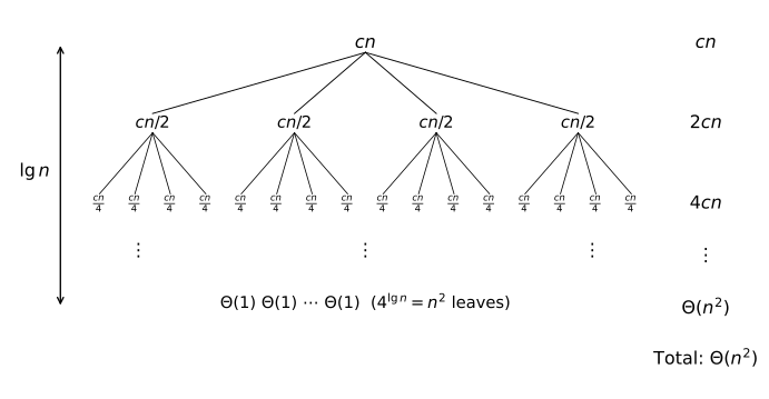
\begin{equation*} \begin{aligned} T(n) &= \sum_{i=0}^{\lg n - 1} 2^i cn + \Theta(n^2) \\ &= cn(n-1) + \Theta(n^2) = \Theta(n^2). \end{aligned} \end{equation*}
Substitution, upper bound. Claim \(T(n) \le dn^2 - 2cn\) for all \(n \ge 2\), where \(d = \max\{(T(2)+4c)/4,\ (T(3)+6c)/9\}\). The base cases \(n = 2, 3\) hold by the choice of \(d\). For \(n \ge 4\) we have \(\lfloor n/2 \rfloor \ge 2\), so the hypothesis applies to \(\lfloor n/2 \rfloor\); using \((n-1)/2 \le \lfloor n/2 \rfloor \le n/2\),
\begin{equation*} \begin{aligned} T(n) &\le 4\bigl(d\lfloor n/2\rfloor^2 - 2c\lfloor n/2\rfloor\bigr) + cn \\ &\le dn^2 - 4c(n-1) + cn \\ &= dn^2 - 2cn - (cn - 4c) \le dn^2 - 2cn \qquad (n \ge 4). \end{aligned} \end{equation*}
Substitution, lower bound. Claim \(T(n) \ge d^{\prime}n^2\) for all \(n \ge 1\), where \(d^{\prime} = \min\{c/2,\ T(1)\}\). The base case \(n = 1\) holds since \(d^{\prime} \le T(1)\). For \(n \ge 2\),
\begin{equation*} \begin{aligned} T(n) &\ge 4d^{\prime}\lfloor n/2\rfloor^2 + cn \ge d^{\prime}(n-1)^2 + cn \\ &= d^{\prime}n^2 + \bigl(cn - d^{\prime}(2n-1)\bigr) \ge d^{\prime}n^2, \end{aligned} \end{equation*}
since \(d^{\prime}(2n-1) \le (c/2)(2n) = cn\). Hence \(T(n) = \Theta(n^2)\).
With constants \(a \ge 1\) and \(c > 0\), find an asymptotically tight solution of \(T(n) = T(n-a) + T(a) + cn\) by means of a recursion tree.
\(T(n) = \Theta(n^2)\); in fact \(T(n) = cn^2/(2a) + O(n)\) (taking \(T(n) = \Theta(1)\) for \(0 < n \le a\), so \(T(a)\) is a constant).
For \(n > a\) let \(k = \lceil n/a \rceil - 1 \ge 1\) and \(r = n - ka \in (0, a]\). The recursion tree is a spine: the node at depth \(i\) (\(0 \le i \le k-1\)) has subproblem size \(n - ia\) and cost \(c(n-ia)\), and two children, a leaf \(T(a)\) and the next spine node \(T(n-(i+1)a)\); the spine ends at depth \(k\) in the leaf \(T( r)\). Summing the tree, and writing \(n - ia = r + (k-i)a\),
\begin{equation*} \begin{aligned} T(n) &= c\sum_{i=0}^{k-1}(n - ia) + kT(a) + T( r) \\ &= c\Bigl(kr + \frac{a\,k(k+1)}{2}\Bigr) + kT(a) + T( r). \end{aligned} \end{equation*}
Since \(n/a - 1 \le k \le n/a\), \(0 < r \le a\) and \(T( r) = \Theta(1)\),
\begin{equation*} \frac{c\,n(n-a)}{2a} \le T(n) \le \frac{c\,n(n+a)}{2a} + cn + \frac{n}{a}T(a) + O(1). \end{equation*}
Both sides are \(cn^2/(2a) + O(n)\) (\(a\) and \(c\) are constants), so \(T(n) = \Theta(n^2)\).
Let \(\alpha\) be a constant with \(0 < \alpha < 1\) and let \(c > 0\) be a constant. Using a recursion tree, find an asymptotically tight solution of \(T(n) = T(\alpha n) + T((1-\alpha)n) + cn\).
\(T(n) = \Theta(n \lg n)\) (taking \(T(n) = \Theta(1)\), positive, for \(n < 1\), and the recurrence for \(n \ge 1\)).
Put \(\beta = \min\{\alpha, 1-\alpha\}\) and \(\gamma = \max\{\alpha, 1-\alpha\}\), so \(0 < \beta \le 1/2 \le \gamma < 1\). As in Figure 4.6, a node at depth \(i\) has size \(\alpha^j(1-\alpha)^{i-j}n \in [\beta^i n, \gamma^i n]\); a node is internal (cost \(c\) times its size) when its size is \(\ge 1\) and a leaf otherwise. The sizes of the nodes at any depth sum to at most \(n\), with equality as long as no leaf lies above that depth.
Upper bound. Internal nodes have \(\gamma^i n \ge 1\), so they occupy depths \(0 \le i \le \log_{1/\gamma} n\), and each depth costs at most \(cn\). Each leaf has size \(\ge \beta\) (its parent has size \(\ge 1\)), and the leaves partition the root’s size \(n\), so there are at most \(n/\beta\) leaves. Hence
\begin{equation*} T(n) \le cn\bigl(\log_{1/\gamma} n + 1\bigr) + \frac{n}{\beta}\,\Theta(1) = O(n \lg n). \end{equation*}
Lower bound. For \(0 \le i \le \log_{1/\beta} n\) every node at depth \(i\) has size \(\ge \beta^i n \ge 1\), so these depths are complete levels of internal nodes, each costing exactly \(cn\). Hence
\begin{equation*} T(n) \ge cn\bigl(\lfloor \log_{1/\beta} n \rfloor + 1\bigr) \ge \frac{c}{\lg(1/\beta)}\, n \lg n = \Omega(n \lg n). \end{equation*}
Therefore \(T(n) = \Theta(n \lg n)\).
4.5 The master method for solving recurrences
Give tight asymptotic bounds, via the master method, for each recurrence: (a) \(T(n) = 2T(n/4) + 1\); (b) \(T(n) = 2T(n/4) + \sqrt{n}\); (c) \(T(n) = 2T(n/4) + n\); (d) \(T(n) = 2T(n/4) + n^2\).
(a) \(\Theta(\sqrt n)\), (b) \(\Theta(\sqrt n\lg n)\), (c) \(\Theta(n)\), (d) \(\Theta(n^2)\). In all four, \(a=2\), \(b=4\), so \(n^{\log_b a} = n^{\log_4 2} = n^{1/2}\), and Theorem 4.1 gives:
(a) \(f(n) = 1 = O(n^{1/2-\epsilon})\) with \(\epsilon = 1/2\): case 1, \(T(n) = \Theta(\sqrt n)\).
(b) \(f(n) = \sqrt n = \Theta(n^{1/2})\): case 2, \(T(n) = \Theta(\sqrt n \lg n)\).
(c) \(f(n) = n = \Omega(n^{1/2+\epsilon})\) with \(\epsilon = 1/2\), and regularity holds with \(c = 1/2\): \[ af(n/b) = 2\cdot\frac n4 = \frac12\, n = c f(n). \] Case 3: \(T(n) = \Theta(n)\).
(d) \(f(n) = n^2 = \Omega(n^{1/2+\epsilon})\) with \(\epsilon = 3/2\), and regularity holds with \(c = 1/8\): \[ af(n/b) = 2\left(\frac n4\right)^2 = \frac18\, n^2 = c f(n). \] Case 3: \(T(n) = \Theta(n^2)\).
Professor Caesar plans a divide-and-conquer matrix-multiplication algorithm that splits each \(n\times n\) matrix into blocks of size \(n/4 \times n/4\), recurses on \(a\) subproblems, and spends \(\Theta(n^2)\) time on dividing and combining, so that \(T(n) = aT(n/4) + \Theta(n^2)\). What is the largest integer \(a\) for which his algorithm is asymptotically faster than Strassen’s algorithm, whose running time is \(\Theta(n^{\lg 7})\)?
\(a = 48\). Here \(n^{\log_b a} = n^{\log_4 a}\), and the threshold is \[ \log_4 a = \lg 7 \iff a = 4^{\lg 7} = (2^{\lg 7})^2 = 49 . \] (i) \(a = 48\): \(\log_4 48 \approx 2.79\), so \(f(n) = \Theta(n^2) = O(n^{\log_4 48 - \epsilon})\) with \(\epsilon = \log_4 48 - 2 > 0\); case 1 of Theorem 4.1 gives \(T(n) = \Theta(n^{\log_4 48})\), and \(\log_4 48 < \log_4 49 = \lg 7\), so \(T(n) = o(n^{\lg 7})\).
(ii) \(a \ge 49\): \(\log_4 a \ge \lg 7 > 2\), so again case 1 applies and \(T(n) = \Theta(n^{\log_4 a}) = \Omega(n^{\lg 7})\), which is not asymptotically faster than Strassen.
Show with the master method that the binary-search recurrence \(T(n) = T(n/2) + \Theta(1)\) has solution \(T(n) = \Theta(\lg n)\). (Binary search is described in Exercise 2.3-5.)
Case 2 of Theorem 4.1 applies: with \(a = 1 \ge 1\), \(b = 2 > 1\), \[ n^{\log_b a} = n^{\log_2 1} = 1, \qquad f(n) = \Theta(1) = \Theta(n^{\log_b a}), \] so \(T(n) = \Theta(n^{\log_b a}\lg n) = \Theta(\lg n)\).
Does the master method apply to \(T(n) = 4T(n/2) + n^2\lg n\)? Explain why or why not, and give an asymptotic upper bound for this recurrence.
No; but \(T(n) = O(n^2\lg^2 n)\) (in fact \(\Theta(n^2\lg^2 n)\)). Here \(a = 4\), \(b = 2\), \(n^{\log_b a} = n^2\), and \[ \frac{f(n)}{n^{\log_b a}} = \lg n = \omega(1), \qquad \lg n = o(n^{\epsilon})\ \ (\epsilon > 0) . \] So \(f(n)\) is neither \(O(n^{2-\epsilon})\) (case 1) nor \(\Theta(n^2)\) (case 2) nor \(\Omega(n^{2+\epsilon})\) (case 3): \(f\) is larger than \(n^{\log_b a}\) but not polynomially larger, the gap between cases 2 and 3.
For the bound, take \(n = 2^k\) and sum the recursion tree exactly, as in Lemma 4.2: level \(j\) has \(4^j\) nodes of cost \((n/2^j)^2\lg(n/2^j) = 4^{k-j}(k-j)\), and there are \(4^k = n^2\) leaves, so
\begin{equation*} \begin{aligned} T(n) &= n^2\,T(1) + \sum_{j=0}^{k-1} 4^j\cdot 4^{k-j}(k-j) = n^2\,T(1) + 4^k\sum_{i=1}^{k} i \\ &= n^2\left(T(1) + \frac{\lg n\,(\lg n+1)}{2}\right) = \Theta(n^2\lg^2 n) . \end{aligned} \end{equation*}
Floors and ceilings are handled as in Section 4.6.2 (see also Exercise 4.6-2), so \(T(n) = O(n^2\lg^2 n)\).
Case 3 of the master theorem includes the regularity condition \(af(n/b) \le cf(n)\) for some constant \(c < 1\). Exhibit constants \(a \ge 1\) and \(b > 1\) and a function \(f(n)\) that meet every condition of case 3 except the regularity condition.
Take \(a = 1\), \(b = 2\) and \(f(n) = 4^{\lceil \log_4 n\rceil}\), the least power of 4 that is \(\ge n\). Then \(n^{\log_b a} = n^0 = 1\) and \[ f(n) \ge n = \Omega(n^{\log_b a + \epsilon}) \quad\text{with } \epsilon = 1, \] so the growth condition of case 3 holds. But for every \(n = 4^k\) with \(k \ge 1\), the argument \(n/2 = 2\cdot 4^{k-1}\) is an integer (so floors and ceilings change nothing) lying in \((4^{k-1}, 4^k]\), hence \[ af(n/b) = f(2\cdot 4^{k-1}) = 4^k = f(n) > cf(n) \quad\text{for every } c < 1 , \] for arbitrarily large \(n\), so regularity fails.
4.6 Proof of the master theorem
Equation (4.27) defines the arguments in the recursion tree of \(T(n) = aT(\lceil n/b \rceil) + f(n)\) by \(n_0 = n\) and \(n_j = \lceil n_{j-1}/b \rceil\) for \(j > 0\). When \(b\) is a positive integer (rather than an arbitrary real \(b > 1\)), find a simple, exact closed form for \(n_j\).
\(n_j = \lceil n/b^j \rceil\) for every \(j \ge 0\).
By induction on \(j\): the case \(j = 0\) is \(n_0 = n = \lceil n/b^0 \rceil\) (\(n\) is an integer), and if \(n_{j-1} = \lceil n/b^{j-1} \rceil\) then equation (3.4), \(\lceil \lceil x/a \rceil / b \rceil = \lceil x/(ab) \rceil\) for real \(x \ge 0\) and positive integers \(a, b\), applied with \(x = n\) and \(a = b^{j-1}\) (a positive integer because \(b\) is) gives
\begin{equation*} n_j = \left\lceil \frac{\lceil n/b^{j-1} \rceil}{b} \right\rceil = \left\lceil \frac{n}{b^{j}} \right\rceil . \end{equation*}
Suppose \(f(n) = \Theta(n^{\log_b a} \lg^k n)\) for a constant \(k \ge 0\). Prove that the master recurrence \(T(n) = aT(n/b) + f(n)\) then has solution \(T(n) = \Theta(n^{\log_b a} \lg^{k+1} n)\). You may restrict attention to \(n\) an exact power of \(b\).
Write \(p = \log_b a\), \(n = b^L\), and sum the recursion tree: by Lemma 4.2 (whose hypothesis is that \(f\) is nonnegative, as a driving function of the master recurrence is),
\begin{equation*} T(n) = \Theta(n^{p}) + \sum_{j=0}^{L-1} a^j f(b^{L-j}) . \end{equation*}
By hypothesis there are constants \(c_1, c_2 > 0\) and an integer \(i_0 \ge 1\) with \(c_1 m^p \lg^k m \le f(m) \le c_2 m^p \lg^k m\) for all \(m = b^i\), \(i \ge i_0\). Since \(a^j (b^{L-j})^p = a^j a^{L-j} = n^p\) and \(\lg b^{i} = i \lg b\), splitting the sum at \(i = L - j = i_0\) gives
\begin{equation*} \begin{aligned} \sum_{j=0}^{L-1} a^j f(b^{L-j}) &= \Theta\Big(n^p \lg^k b \sum_{i=i_0}^{L} i^k\Big) + \sum_{i=1}^{i_0-1} a^{L-i} f(b^{i}) \\ &= \Theta\Big(n^p \sum_{i=i_0}^{L} i^k\Big) + O(n^p), \end{aligned} \end{equation*}
because the second sum has \(i_0 - 1\) terms, each at most \(a^L \max_{i < i_0} f(b^i) = O(n^p)\). Finally, for \(L \ge 2 i_0\) (using \(k \ge 0\)),
\begin{equation*} \begin{aligned} \Big(\frac{L}{2}\Big)^{k+1} &\le \sum_{\lceil L/2 \rceil \le i \le L} i^k \\ &\le \sum_{i=i_0}^{L} i^k \le L \cdot L^k = L^{k+1}, \end{aligned} \end{equation*}
so the sum is \(\Theta(L^{k+1}) = \Theta(\lg^{k+1} n)\), as \(L = \lg n / \lg b\). Hence
\begin{equation*} \begin{aligned} T(n) &= \Theta(n^p) + \Theta(n^p \lg^{k+1} n) + O(n^p) \\ &= \Theta(n^{\log_b a} \lg^{k+1} n), \end{aligned} \end{equation*}
the last step because \(\lg^{k+1} n \ge 1\) for \(n \ge 2\).
Case 3 of the master theorem assumes both \(f(n) = \Omega(n^{\log_b a + \epsilon})\) for some \(\epsilon > 0\) and the regularity condition. Show that the first assumption is redundant: if \(af(n/b) \le cf(n)\) for some constant \(c < 1\) (and all sufficiently large \(n\)), then \(f(n) = \Omega(n^{\log_b a + \epsilon})\) for some constant \(\epsilon > 0\).
Take \(\epsilon = \log_b(1/c)\), which is positive because \(b > 1\) and \(0 < c < 1\) (\(c > 0\) since \(af(n/b) > 0\) for large \(n\)); then \(a/c = b^{\log_b a + \epsilon} > 1\).
As in Theorem 4.1, \(n/b\) means \(\lfloor n/b \rfloor\) or \(\lceil n/b \rceil\), so \(f\) lives on the integers. Fix \(N\) with regularity holding and \(f > 0\) on all integers \(m \ge N/b - 1\), and let \(d > 0\) be the minimum of \(f\) over the finitely many integers in \([N/b - 1, N)\). For \(n \ge N\) iterate \(m_0 = n\), \(m_{i+1} = m_i/b\) (rounded), and let \(J\) be the first index with \(m_J < N\); then \(m_J \ge N/b - 1\). Unrolling the nested roundings as in Section 4.6.2 gives \(m_J > n/b^J - b/(b-1)\), so \(b^J > n/K\) with \(K = N + b/(b-1)\). Applying \(f(m_i) \ge (a/c) f(m_{i+1})\) for \(i < J\) (each \(m_i \ge N\)),
\begin{equation*} \begin{aligned} f(n) &\ge \Big(\frac{a}{c}\Big)^{J} f(m_J) \ge d \, (b^J)^{\log_b a + \epsilon} \\ &\ge \frac{d}{K^{\log_b a + \epsilon}} \, n^{\log_b a + \epsilon} , \end{aligned} \end{equation*}
so \(f(n) = \Omega(n^{\log_b a + \epsilon})\).
Problems for Chapter 4
Recurrence examples: for each recurrence below, find asymptotic upper and lower bounds on \(T(n)\), as tight as you can, and justify them. Take \(T(n)\) to be constant whenever \(n \le 2\).
(a) \(T(n) = 2T(n/2) + n^4\).
(b) \(T(n) = T(7n/10) + n\).
(c) \(T(n) = 16T(n/4) + n^2\).
(d) \(T(n) = 7T(n/3) + n^2\).
(e) \(T(n) = 7T(n/2) + n^2\).
(f) \(T(n) = 2T(n/4) + \sqrt{n}\).
(g) \(T(n) = T(n-2) + n^2\).
All bounds are tight: (a) \(\Theta(n^4)\), (b) \(\Theta(n)\), (c) \(\Theta(n^2\lg n)\), (d) \(\Theta(n^2)\), (e) \(\Theta(n^{\lg 7})\), (f) \(\Theta(\sqrt{n}\lg n)\), (g) \(\Theta(n^3)\). Parts (a) to (f) use the master theorem (Theorem 4.1) with \(a \ge 1\), \(b > 1\) in each case.
(a) \(a=b=2\), \(n^{\log_b a} = n\), and \(f(n) = n^4 = \Omega(n^{1+3})\). Regularity: \(2(n/2)^4 = n^4/8 \le \tfrac18 f(n)\). Case 3 gives \(T(n) = \Theta(n^4)\).
(b) \(a=1\), \(b = 10/7\), \(n^{\log_b a} = n^0 = 1\), and \(f(n) = n = \Omega(n^{0+1})\). Regularity: \(7n/10 \le \tfrac{7}{10} f(n)\). Case 3 gives \(T(n) = \Theta(n)\).
(c) \(a=16\), \(b=4\), \(n^{\log_4 16} = n^2\) and \(f(n) = n^2 = \Theta(n^2)\). Case 2 gives \(T(n) = \Theta(n^2 \lg n)\).
(d) \(a=7\), \(b=3\), \(\log_3 7 \approx 1.77 < 2\), so \(f(n) = n^2 = \Omega(n^{\log_3 7 + \epsilon})\) with \(\epsilon = 2 - \log_3 7 > 0\). Regularity: \(7(n/3)^2 = \tfrac79 f(n)\). Case 3 gives \(T(n) = \Theta(n^2)\).
(e) \(a=7\), \(b=2\), \(\lg 7 \approx 2.81 > 2\), so \(f(n) = n^2 = O(n^{\lg 7 - \epsilon})\) with \(\epsilon = \lg 7 - 2 > 0\). Case 1 gives \(T(n) = \Theta(n^{\lg 7})\).
(f) \(a=2\), \(b=4\), \(n^{\log_4 2} = n^{1/2}\) and \(f(n) = \sqrt{n} = \Theta(n^{1/2})\). Case 2 gives \(T(n) = \Theta(\sqrt{n}\lg n)\).
(g) The master theorem does not apply; unroll instead. Let \(k = \lceil (n-2)/2 \rceil\) be the number of steps that bring the argument down to at most \(2\), and let \(c = \max_{m \le 2} T(m)\). Then
\begin{equation*} T(n) = T(n-2k) + \sum_{j=0}^{k-1} (n-2j)^2 . \end{equation*}
Upper bound: there are \(k \le n/2\) terms, each at most \(n^2\), so \(T(n) \le c + n^3/2\). Lower bound: for \(n \ge 8\) we have \(k - 1 \ge n/2 - 2 \ge n/4\), so the sum includes every \(j\) with \(0 \le j \le n/4\). That is at least \(n/4\) terms, and each has \(n - 2j \ge n/2\), so
\begin{equation*} T(n) \ge \frac{n}{4}\Big(\frac{n}{2}\Big)^2 = \frac{n^3}{16}. \end{equation*}
Hence \(T(n) = \Theta(n^3)\).
Parameter-passing costs: the book normally charges constant time to pass a parameter to a procedure, even an \(N\)-element array, because in most systems only a pointer to the array is passed. This problem compares three ways of passing an array:
(1) by pointer, at cost \(\Theta(1)\); (2) by copying the whole array, at cost \(\Theta(N)\), where \(N\) is the array’s size; (3) by copying only the subrange the callee might touch, at cost \(\Theta(q-p+1)\) when the subarray \(A[p \,.\,.\, q]\) is passed.
(a) For the recursive binary search for a number in a sorted array (Exercise 2.3-5), write recurrences for the worst-case running time under each of the three methods, and give good upper bounds on their solutions. Use \(N\) for the size of the original problem and \(n\) for the size of a subproblem.
(b) Do the same as in (a) for MERGE-SORT from Section 2.3.1.
(a) Binary search costs \(\Theta(\lg N)\), \(\Theta(N\lg N)\) and \(\Theta(N)\) under methods 1, 2 and 3. Each call does \(\Theta(1)\) work, then makes at most one recursive call on a subarray of size at most \(\lfloor n/2 \rfloor\). In the worst case (an unsuccessful search) the recursion goes all the way down. So the recurrences are:
(i) Pointer: \(T(n) = T(n/2) + \Theta(1)\). Case 2 of Theorem 4.1 (\(a=1\), \(b=2\), \(n^{\log_2 1} = 1\)) gives \(T(N) = \Theta(\lg N)\).
(ii) Full copy: \(T(n) = T(n/2) + \Theta(N)\), where \(N\) is a constant throughout the recursion. With \(T(n) \le T(n/2) + cN\) there are \(\lfloor \lg n \rfloor + 1\) levels, so
\begin{equation*} T(N) \le cN(\lg N + 1) + O(1) = O(N \lg N), \end{equation*}
and the same count with a lower constant gives \(\Omega(N\lg N)\). Hence \(T(N) = \Theta(N\lg N)\).
(iii) Subrange copy: copying the half of size about \(n/2\) costs \(\Theta(n)\), so \(T(n) = T(n/2) + \Theta(n)\). Here \(f(n) = n = \Omega(n^{0+1})\) and the regularity condition holds, since \(f(n/2) = \tfrac12 f(n)\). Case 3 of Theorem 4.1 gives \(T(N) = \Theta(N)\).
(b) Merge sort costs \(\Theta(N\lg N)\), \(\Theta(N^2)\) and \(\Theta(N\lg N)\) under methods 1, 2 and 3. A call on \(n > 1\) elements makes two recursive calls on halves and one call to MERGE, which does \(\Theta(n)\) work on top of what it costs to pass the array.
(i) Pointer: \(T(n) = 2T(n/2) + \Theta(n)\). Case 2 of Theorem 4.1 gives \(T(N) = \Theta(N\lg N)\).
(ii) Full copy: each of the three calls costs \(\Theta(N)\) to pass the array, so \(T(n) = 2T(n/2) + \Theta(n) + \Theta(N)\). Take \(n = 2^k\) with \(T(n) = 2T(n/2) + cn + dN\). Level \(i\) of the recursion tree has \(2^i\) nodes, each costing \(c\,n/2^i + dN\), and there are \(n\) leaves. So
\begin{equation*} \begin{aligned} T(n) &= \sum_{i=0}^{k-1} \big(cn + 2^i dN\big) + n\,T(1) \\ &= cn\lg n + dN(n-1) + \Theta(n). \end{aligned} \end{equation*}
Setting \(n = N\) gives \(T(N) = \Theta(N^2)\).
(iii) Subrange copy: passing \(A[p \,.\,.\, q]\) to the two recursive calls and to MERGE costs \(\Theta(n)\) in total. So \(T(n) = 2T(n/2) + \Theta(n)\), the same recurrence as in (i), and \(T(N) = \Theta(N\lg N)\).
More recurrence examples: for each recurrence below, give asymptotic upper and lower bounds on \(T(n)\), as tight as you can, and justify them. Take \(T(n)\) to be constant for all sufficiently small \(n\).
(a) \(T(n) = 4T(n/3) + n\lg n\).
(b) \(T(n) = 3T(n/3) + n/\lg n\).
(c) \(T(n) = 4T(n/2) + n^2\sqrt{n}\).
(d) \(T(n) = 3T(n/3 - 2) + n/2\).
(e) \(T(n) = 2T(n/2) + n/\lg n\).
(f) \(T(n) = T(n/2) + T(n/4) + T(n/8) + n\).
(g) \(T(n) = T(n-1) + 1/n\).
(h) \(T(n) = T(n-1) + \lg n\).
(i) \(T(n) = T(n-2) + 1/\lg n\).
(j) \(T(n) = \sqrt{n}\,T(\sqrt{n}) + n\).
All ten bounds are tight: (a) \(\Theta(n^{\log_3 4})\), (b) \(\Theta(n\lg\lg n)\), (c) \(\Theta(n^{5/2})\), (d) \(\Theta(n\lg n)\), (e) \(\Theta(n\lg\lg n)\), (f) \(\Theta(n)\), (g) \(\Theta(\lg n)\), (h) \(\Theta(n\lg n)\), (i) \(\Theta(n/\lg n)\), (j) \(\Theta(n\lg\lg n)\).
(a) Here \(a=4\), \(b=3\), \(n^{\log_3 4} \approx n^{1.262}\). Since \(\lg n = O(n^{0.1})\), \(f(n) = n\lg n = O(n^{\log_3 4 - \epsilon})\) with \(\epsilon = 0.1\), so case 1 of the master theorem (Theorem 4.1) gives \(T(n) = \Theta(n^{\log_3 4})\).
(b) The master theorem does not apply: \(n/\lg n\) is \(o(n)\) but not \(O(n^{1-\epsilon})\). Take \(n = 3^k\). By Lemma 4.2 (with \(f\) only evaluated at \(n/3^j\), \(j \le k-1\), so never at \(1\)),
\begin{equation*} \begin{aligned} T(n) &= \Theta(n) + \sum_{j=0}^{k-1} 3^j \frac{n/3^j}{\lg(n/3^j)} = \Theta(n) + \sum_{j=0}^{k-1} \frac{n}{(k-j)\lg 3} \\ &= \Theta(n) + \frac{n}{\lg 3} H_k = \Theta(n) + \frac{n}{\lg 3}\bigl(\ln k + O(1)\bigr) = \Theta(n\lg\lg n), \end{aligned} \end{equation*}
using \(H_k = \ln k + O(1)\) (equation (A.7)) and \(k = \log_3 n\). For general \(n\), \(T\) is nondecreasing (as it is for any reasonable reading with floors or ceilings), and sandwiching \(3^k \le n < 3^{k+1}\) changes \(n\lg\lg n\) by at most a constant factor.
(c) Here \(n^{\log_2 4} = n^2\) and \(f(n) = n^{5/2} = \Omega(n^{2+\epsilon})\) with \(\epsilon = 1/2\). Regularity: \(4f(n/2) = 4(n/2)^{5/2} = n^{5/2}/\sqrt{2}\), so \(af(n/b) \le c f(n)\) with \(c = 1/\sqrt{2} < 1\). Case 3 of Theorem 4.1 gives \(T(n) = \Theta(n^{5/2})\).
(d) \(T(n) = \Theta(n\lg n)\), by substitution. Fix the base region as \(2 \le n < 12\), where \(C^{\prime} \le T(n) \le C\) for positive constants (any bounded range of arguments has bounded, positive \(T\)); for \(n \ge 12\) the argument \(m = n/3 - 2\) satisfies \(n/6 \le m < n\) and \(m \ge 2\), and arguments drop by at least \(2\) per step, so induction on \(n\) is valid.
Upper bound: claim \(T(n) \le c\,n\lg n\) for \(n \ge 2\) with \(c = \max(C, 1/(2\lg 3))\). Base: \(T(n) \le C \le c\,n\lg n\) as \(n\lg n \ge 2\). Step (\(n \ge 12\), so \(n - 6 \ge 0\) and \(\lg(n/3) \ge 0\)):
\begin{equation*} \begin{aligned} T(n) &\le 3c\,m\lg m + n/2 \le c(n-6)\lg(n/3) + n/2 \\ &\le c\,n\lg n - (c\lg 3 - 1/2)\,n \le c\,n\lg n. \end{aligned} \end{equation*}
Lower bound: claim \(T(n) \ge d\,n\lg n\) for \(n \ge 2\) with \(d = \min\bigl(C^{\prime}/(12\lg 12),\ 1/(2(\lg 6 + 1))\bigr)\). Base: \(T(n) \ge C^{\prime} \ge d\,n\lg n\) for \(n < 12\). Step, using \(m \ge n/6\) and \(\lg(n/6) \le n/6\):
\begin{equation*} \begin{aligned} T(n) &\ge 3d\,m\lg m + n/2 \ge d(n-6)\lg(n/6) + n/2 \\ &= d\,n\lg n - d\,n\lg 6 - 6d\lg(n/6) + n/2 \\ &\ge d\,n\lg n - \bigl(d(\lg 6 + 1) - 1/2\bigr)n \ge d\,n\lg n. \end{aligned} \end{equation*}
(e) The same computation as (b) with \(a = b = 2\) and \(n = 2^k\): by Lemma 4.2,
\begin{equation*} T(n) = \Theta(n) + \sum_{j=0}^{k-1} \frac{n}{k-j} = \Theta(n) + nH_k = \Theta(n\lg\lg n), \end{equation*}
since \(k = \lg n\) and \(H_k = \ln k + O(1)\) by (A.7); monotonicity extends this to all \(n\) as in (b).
(f) \(T(n) = \Theta(n)\). The lower bound \(T(n) \ge n\) is immediate. For the upper bound claim \(T(n) \le c\,n\) for \(n \ge 1\), with \(c \ge 8\) large enough to cover the base cases; then
\begin{equation*} T(n) \le c\frac{n}{2} + c\frac{n}{4} + c\frac{n}{8} + n = \frac{7c}{8}n + n \le c\,n \quad\text{since } c \ge 8. \end{equation*}
(g) Unrolling down to the constant base value \(T(n_0)\),
\begin{equation*} T(n) = T(n_0) + \sum_{k=n_0+1}^{n} \frac{1}{k} = H_n - H_{n_0} + O(1) = \ln n + O(1) = \Theta(\lg n) \end{equation*}
by (A.7).
(h) Unrolling likewise,
\begin{equation*} T(n) = T(n_0) + \sum_{k=n_0+1}^{n} \lg k = \lg(n!) + O(1) = \Theta(n\lg n) \end{equation*}
by equation (3.19).
(i) \(T(n) = \Theta(n/\lg n)\). Take \(T\) constant for \(n < 4\). Unrolling gives \(T(n) = \Theta(1) + \sum_{k \in K} 1/\lg k\) with \(K = \{n, n-2, n-4, \ldots\} \cap [4, n]\), and \((n-4)/2 \le |K| \le n/2\). Each term is at least \(1/\lg n\), so the sum is at least \((n-4)/(2\lg n)\). For the upper bound, split at \(\sqrt{n}\): terms with \(k \le \sqrt{n}\) are at most \(1/2\) each (as \(\lg k \ge 2\)), and terms with \(k > \sqrt{n}\) satisfy \(1/\lg k < 2/\lg n\), so
\begin{equation*} \sum_{k \in K} \frac{1}{\lg k} \le \frac{\sqrt{n}}{2} + \frac{n}{2}\cdot\frac{2}{\lg n} = O\!\left(\frac{n}{\lg n}\right). \end{equation*}
(j) \(T(n) = \Theta(n\lg\lg n)\). Divide by \(n\): \(S(n) = T(n)/n\) satisfies \(S(n) = S(\sqrt{n}) + 1\). Let \(T\) be constant for \(n \le n_0\), where \(n_0 > 1\), and let \(k\) be the least integer with \(n^{1/2^k} \le n_0\), that is,
\begin{equation*} k = \bigl\lceil \lg\lg n - \lg\lg n_0 \bigr\rceil . \end{equation*}
Iterating \(k\) times gives \(S(n) = k + S(m)\) with \(m = n^{1/2^k} \in (\sqrt{n_0}, n_0]\), a fixed bounded interval on which \(T(m)/m\) is bounded above and below by positive constants. Hence \(S(n) = \lg\lg n + \Theta(1)\), so \(T(n) = n\lg\lg n + \Theta(n) = \Theta(n\lg\lg n)\).
Fibonacci numbers: this problem studies the Fibonacci numbers \(F_i\) of recurrence (3.22) through generating functions. Let \(\mathcal{F}\) be the generating function (formal power series)
\begin{equation*} \begin{aligned} \mathcal{F}(z) &= \sum_{i=0}^{\infty} F_i z^i \\ &= 0 + z + z^2 + 2z^3 + 3z^4 + 5z^5 + 8z^6 + 13z^7 + 21z^8 + \cdots . \end{aligned} \end{equation*}
(a) Prove that \(\mathcal{F}(z) = z + z\mathcal{F}(z) + z^2\mathcal{F}(z)\).
(b) Prove that
\begin{equation*} \begin{aligned} \mathcal{F}(z) &= \frac{z}{1 - z - z^2} = \frac{z}{(1-\phi z)(1-\hat\phi z)} \\ &= \frac{1}{\sqrt5}\left(\frac{1}{1-\phi z} - \frac{1}{1-\hat\phi z}\right), \end{aligned} \end{equation*}
where \(\phi = (1+\sqrt5)/2 = 1.61803\ldots\) and \(\hat\phi = (1-\sqrt5)/2 = -0.61803\ldots\).
(c) Prove that
\begin{equation*} \mathcal{F}(z) = \sum_{i=0}^{\infty} \frac{1}{\sqrt5}\bigl(\phi^i - \hat\phi^i\bigr) z^i . \end{equation*}
(d) Deduce from (c) that for \(i > 0\), \(F_i\) equals \(\phi^i/\sqrt5\) rounded to the nearest integer. (Hint: \(|\hat\phi| < 1\).)
The generating function is \(\mathcal{F}(z) = z/(1-z-z^2)\), which gives \(F_i = (\phi^i - \hat\phi^i)/\sqrt5\), the integer nearest to \(\phi^i/\sqrt5\).
(a) Shift indices and use \(F_0 = 0\), \(F_1 = 1\) and \(F_i = F_{i-1} + F_{i-2}\) for \(i \ge 2\) (recurrence (3.22)):
\begin{equation*} \begin{aligned} z + z\mathcal{F}(z) + z^2\mathcal{F}(z) &= z + \sum_{i \ge 1} F_{i-1} z^i + \sum_{i \ge 2} F_{i-2} z^i \\ &= z + F_0 z + \sum_{i \ge 2} (F_{i-1} + F_{i-2}) z^i \\ &= F_0 + F_1 z + \sum_{i \ge 2} F_i z^i = \mathcal{F}(z). \end{aligned} \end{equation*}
(b) By (a), \(\mathcal{F}(z)(1 - z - z^2) = z\). The series \(1 - z - z^2\) has constant term \(1\), so it is invertible in the ring of formal power series, and \(\mathcal{F}(z) = z/(1-z-z^2)\). Since \(\phi\) and \(\hat\phi\) are the roots of \(x^2 = x + 1\), we have \(\phi + \hat\phi = 1\) and \(\phi\hat\phi = -1\), hence
\begin{equation*} (1-\phi z)(1-\hat\phi z) = 1 - (\phi+\hat\phi)z + \phi\hat\phi z^2 = 1 - z - z^2 , \end{equation*}
which is the second equality. For the third, \(\phi - \hat\phi = \sqrt5\) gives
\begin{equation*} \frac{1}{1-\phi z} - \frac{1}{1-\hat\phi z} = \frac{(1-\hat\phi z) - (1-\phi z)}{(1-\phi z)(1-\hat\phi z)} = \frac{\sqrt5\, z}{(1-\phi z)(1-\hat\phi z)} . \end{equation*}
(c) For any constant \(\alpha\), \((1-\alpha z)\sum_{i\ge0}\alpha^i z^i = 1\) (the sum telescopes), so \(1/(1-\alpha z) = \sum_{i \ge 0} \alpha^i z^i\) as formal series. Applying this with \(\alpha = \phi\) and \(\alpha = \hat\phi\) in the last form of (b),
\begin{equation*} \mathcal{F}(z) = \frac{1}{\sqrt5}\left(\sum_{i\ge0}\phi^i z^i - \sum_{i\ge0}\hat\phi^i z^i\right) = \sum_{i \ge 0} \frac{1}{\sqrt5}\bigl(\phi^i - \hat\phi^i\bigr) z^i . \end{equation*}
(d) Two formal power series are equal exactly when their coefficients agree, so comparing the coefficient of \(z^i\) in (c) with the definition of \(\mathcal{F}\) gives \(F_i = (\phi^i - \hat\phi^i)/\sqrt5\). Since \(|\hat\phi| < 1\), for \(i > 0\)
\begin{equation*} \left| F_i - \frac{\phi^i}{\sqrt5} \right| = \frac{|\hat\phi|^i}{\sqrt5} < \frac{1}{\sqrt5} < \frac12 . \end{equation*}
So the integer \(F_i\) lies strictly within \(1/2\) of \(\phi^i/\sqrt5\), which means it is that number rounded to the nearest integer.
Chip testing: Professor Diogenes owns \(n\) integrated-circuit chips, meant to be identical, which can test one another. His jig holds two chips at once; when loaded, each chip tests the other and reports “good” or “bad”. A good chip always reports the other chip’s status correctly; a bad chip’s report is arbitrary. The four possible outcomes are:
| Chip \(A\) says | Chip \(B\) says | Conclusion |
|---|---|---|
| \(B\) is good | \(A\) is good | both are good, or both are bad |
| \(B\) is good | \(A\) is bad | at least one is bad |
| \(B\) is bad | \(A\) is good | at least one is bad |
| \(B\) is bad | \(A\) is bad | at least one is bad |
(a) Show that if at least \(n/2\) of the chips are bad, then no strategy based on such pairwise tests can be guaranteed to determine which chips are good, assuming the bad chips may conspire to fool the professor.
(b) Consider finding one good chip among \(n\) chips, assuming more than \(n/2\) of them are good. Show that \(\lfloor n/2 \rfloor\) pairwise tests suffice to reduce the problem to one of nearly half the size.
(c) Show that, assuming more than \(n/2\) of the chips are good, the good chips can be identified with \(\Theta(n)\) pairwise tests. Give and solve the recurrence for the number of tests.
(a) Let \(G\), \(B\) be the true good and bad sets, \(|B| \ge n/2\), \(n \ge 2\). The bad chips pick \(G^{\prime} \subseteq B\) with \(G^{\prime} \ne G\) and \(|G^{\prime}| \le n/2\), and every bad chip answers as if \(G^{\prime}\) were the good set; then the professor sees the same answers in the true world and in the world with good set \(G^{\prime}\). Such a \(G^{\prime}\) exists:
(i) if \(G \ne \emptyset\), take any \(G^{\prime} \subseteq B\) with \(|G^{\prime}| = |G| \le n/2 \le |B|\); it is nonempty and disjoint from \(G\), so \(G^{\prime} \ne G\);
(ii) if \(G = \emptyset\), take \(G^{\prime} = \{c\}\) for any chip \(c\); \(1 \le n/2\).
In the real world a chip in \(G\) says “good” exactly about chips of \(G\) (truthfully), and every chip of \(B\) says “good” exactly about chips of \(G^{\prime}\). In the world with good set \(G^{\prime}\), the chips of \(G^{\prime} \subseteq B\) answer by that same rule, which is now truthful, while all other chips (\(G\) and \(B \setminus G^{\prime}\)) are bad there and may give any answers, in particular the answers above. This world also satisfies the hypothesis, since it has \(n - |G^{\prime}| \ge n/2\) bad chips. So every test turns out the same in both worlds, and the professor cannot tell whether the good set is \(G\) or \(G^{\prime} \ne G\).
(b) Split the chips into \(\lfloor n/2 \rfloor\) disjoint pairs, leaving one chip \(x\) over if \(n\) is odd, and test each pair. Throw away every pair in which either chip says “bad”, and keep one chip from each pair in which both say “good”. If \(n\) is odd, keep \(x\) exactly when the number of kept chips is even. The kept set has more good chips than bad ones and at most \(\lceil n/2 \rceil\) chips.
A pair containing a good chip and a bad chip is always thrown away, because the good chip says “bad”. Let \(a\) be the number of good-good pairs and \(b\) the number of bad-bad pairs that both say “good”. Let \(m\) be the number of mixed pairs and \(b^{\prime}\) the number of thrown-away bad-bad pairs, and write \([\cdot]\) for an indicator. The kept chips from pairs are \(a\) good and \(b\) bad, and the majority hypothesis reads
\begin{equation*} 2a + m + [x \text{ good}] > 2b + 2b^{\prime} + m + [x \text{ bad}], \quad\text{so}\quad 2a + [x\text{ good}] > 2b + [x \text{ bad}]. \end{equation*}
(i) \(n\) even (no \(x\)): \(a > b\).
(ii) \(x\) good: \(a \ge b\). If \(a+b\) is odd, then \(a \ne b\), so \(a > b\) and \(x\) is dropped. If \(a+b\) is even, \(x\) is kept and \(a + 1 > b\).
(iii) \(x\) bad: \(a > b\). If \(a+b\) is odd, \(x\) is dropped. If \(a+b\) is even, then \(a \ge b+2\), so \(a > b + 1\) with \(x\) kept.
In every case good chips are a strict majority of the kept set, so the set is nonempty. Its size is at most \(a + b + [n \text{ odd}] \le \lceil n/2 \rceil\).
(c) Repeat (b) until one chip is left. That chip is good, because good chips are a strict majority. Next, test it against each of the other \(n-1\) chips; its reports are truthful, so they identify every good chip. With \(T(n)\) the worst-case number of tests in the first phase,
\begin{equation*} T(n) \le T(\lceil n/2 \rceil) + \lfloor n/2 \rfloor \quad (n \ge 2), \qquad T(1) = 0, \end{equation*}
and \(T(n) \le n - 1\) by induction (\(\lceil n/2 \rceil < n\) for \(n \ge 2\)):
\begin{equation*} T(n) \le \bigl(\lceil n/2 \rceil - 1\bigr) + \lfloor n/2 \rfloor = n - 1 . \end{equation*}
So at most \((n-1) + (n-1) = 2n - 2 = O(n)\) tests are used.
For the matching lower bound with \(n \ge 3\), suppose every chip is good, so every report is “good”. If some chip \(c\) is never tested, the world in which only \(c\) is bad gives the same reports and still has \(n - 1 > n/2\) good chips. Hence every chip must be tested, which takes at least \(\lceil n/2 \rceil\) tests, and the total is \(\Theta(n)\).
Monge arrays: An \(m \times n\) array \(A\) of reals is a Monge array if, whenever \(1 \le i < k \le m\) and \(1 \le j < l \le n\),
\begin{equation*} A[i,j] + A[k,l] \le A[i,l] + A[k,j] . \end{equation*}
That is, for any two rows and any two columns, the upper-left plus lower-right entries of the four intersections sum to at most the lower-left plus upper-right entries. For example, this array is Monge:
| 10 | 17 | 13 | 28 | 23 |
|---|---|---|---|---|
| 17 | 22 | 16 | 29 | 23 |
| 24 | 28 | 22 | 34 | 24 |
| 11 | 13 | 6 | 17 | 7 |
| 45 | 44 | 32 | 37 | 23 |
| 36 | 33 | 19 | 21 | 6 |
| 75 | 66 | 51 | 53 | 34 |
(a) Prove that \(A\) is Monge if and only if \(A[i,j] + A[i+1,j+1] \le A[i,j+1] + A[i+1,j]\) for all \(i = 1, \dots, m-1\) and \(j = 1, \dots, n-1\). (Hint: for the “if” direction, induct separately on rows and on columns.)
(b) The array below is not Monge. Change one entry to make it Monge. (Hint: use part (a).)
| 37 | 23 | 22 | 32 |
|---|---|---|---|
| 21 | 6 | 7 | 10 |
| 53 | 34 | 30 | 31 |
| 32 | 13 | 9 | 6 |
| 43 | 21 | 15 | 8 |
(c) Let \(f(i)\) be the column index of the leftmost minimum entry of row \(i\). Prove that \(f(1) \le f(2) \le \cdots \le f(m)\) for every \(m \times n\) Monge array.
(d) A divide-and-conquer algorithm for the leftmost minimum of every row of an \(m \times n\) Monge array \(A\): form the submatrix \(A^{\prime}\) of the even-numbered rows of \(A\), recursively find the leftmost minimum of each row of \(A^{\prime}\), and then find the leftmost minimum of each odd-numbered row of \(A\). Explain how to do this last step in \(O(m+n)\) time, given the leftmost minima of the even-numbered rows.
(e) Write the recurrence for the running time of the algorithm in (d), and show that its solution is \(O(m + n \lg m)\).
(a) The “only if” direction is the special case \(k = i+1\), \(l = j+1\). For “if”, write \(D(r,s) = A[r,s] + A[r+1,s+1] - A[r,s+1] - A[r+1,s]\), which is \(\le 0\) by hypothesis. For \(i < k\) and \(j < l\), the double sum telescopes, first over \(s\) and then over \(r\):
\begin{equation*} \begin{aligned} \sum_{r=i}^{k-1} \sum_{s=j}^{l-1} D(r,s) &= \sum_{r=i}^{k-1} \bigl(A[r,j] + A[r+1,l] - A[r,l] - A[r+1,j]\bigr) \\ &= A[i,j] + A[k,l] - A[i,l] - A[k,j], \end{aligned} \end{equation*}
and the sum is \(\le 0\) because every term is.
(b) Changing \(A[2,3]\) from \(7\) to \(5\) makes the array Monge. The adjacent differences \(D(i,j)\) of part (a) for the given array are
| \(D\) | \(j=1\) | \(j=2\) | \(j=3\) |
|---|---|---|---|
| \(i = 1\) | \(-1\) | \(2\) | \(-7\) |
| \(i = 2\) | \(-4\) | \(-5\) | \(-2\) |
| \(i = 3\) | \(0\) | \(0\) | \(-4\) |
| \(i = 4\) | \(-3\) | \(-2\) | \(-4\) |
The only violation is \(D(1,2) = 23 + 7 - 22 - 6 = 2\). The entry \(A[2,3]\) appears in \(D(1,2)\) and \(D(2,3)\) with sign \(+\), and in \(D(1,3)\) and \(D(2,2)\) with sign \(-\). Lowering it by \(2\) gives
\begin{equation*} D(1,2) = 0,\quad D(2,3) = -4,\quad D(1,3) = -5,\quad D(2,2) = -3, \end{equation*}
so all \(D(i,j) \le 0\), and by (a) the new array is Monge.
(c) Suppose \(f(i) > f(i+1)\) for some \(i\), and put \(j = f(i+1) < l = f(i)\). Since \(l\) is the leftmost minimum of row \(i\) and \(j < l\), we have \(A[i,j] > A[i,l]\). Since \(j\) is a minimum of row \(i+1\), we have \(A[i+1,l] \ge A[i+1,j]\). Adding the two,
\begin{equation*} A[i,j] + A[i+1,l] > A[i,l] + A[i+1,j], \end{equation*}
which contradicts the Monge inequality for rows \(i < i+1\) and columns \(j < l\). Hence \(f(i) \le f(i+1)\) for every \(i\).
(d) For each odd row \(i\), scan row \(i\) only over columns \(f(i-1)\) through \(f(i+1)\), with the conventions \(f(0) = 1\) and \(f(m+1) = n\), and take the leftmost minimum found there.
The answer is correct because \(f(i-1) \le f(i) \le f(i+1)\) by (c), applied to the Monge array \(A\), so the true leftmost minimum \(f(i)\) lies in the scanned range. Any scanned column left of \(f(i)\) holds an entry larger than the row minimum, so the leftmost minimum of the range is \(f(i)\).
Row \(i\) costs \(f(i+1) - f(i-1) + 1\) comparisons. The ranges for consecutive odd rows share only their endpoints, so the total telescopes:
\begin{equation*} \begin{aligned} \sum_{i \text{ odd}} \bigl(f(i+1) - f(i-1) + 1\bigr) &\le f(m+1) - f(0) + \lceil m/2 \rceil \\ &\le n + m = O(m+n). \end{aligned} \end{equation*}
(e) The recursion passes the even rows as a list of row indices, so \(A^{\prime}\) is never copied; copying it would cost \(\Theta(mn)\). For some constant \(c\),
\begin{equation*} T(m,n) \le T(\lfloor m/2 \rfloor, n) + c(m+n) \quad (m \ge 2), \qquad T(1,n) \le cn . \end{equation*}
Claim: \(T(m,n) \le c\,(2m + n + n\lg m)\). The base case holds since \(T(1,n) \le cn \le c(2 + n)\). For \(m \ge 2\), apply the inductive hypothesis to \(\lfloor m/2 \rfloor \ge 1\):
\begin{equation*} \begin{aligned} T(m,n) &\le c\bigl(2\lfloor m/2 \rfloor + n + n \lg(m/2)\bigr) + c(m+n) \\ &\le c\,(m + n\lg m) + c\,(m + n) \\ &= c\,(2m + n + n \lg m). \end{aligned} \end{equation*}
Hence \(T(m,n) = O(m + n + n \lg m)\), which is \(O(m + n\lg m)\) for \(m \ge 2\) (at \(m = 1\) the book’s bound must be read as \(O(m+n)\)).
Chapter 5: Probabilistic Analysis and Randomized Algorithms
5.1 The hiring problem
Line 4 of HIRE-ASSISTANT assumes we can always tell which of two candidates (the current one and the best so far) is the better. Show that this assumption means we know a total order on the ranks of the candidates.
The comparison in line 4 defines a strict relation \(x \succ y\) ("\(x\) is better than \(y\)") that is total, asymmetric and transitive, i.e. a total order (Section B.2), and the ranks are read off from it.
Because HIRE-ASSISTANT must work for every interview order, any two distinct candidates \(x, y\) can arrive as candidates 1 and 2, so line 4 must decide between them: exactly one of \(x \succ y\), \(y \succ x\) holds (totality and asymmetry). Moreover, the variable best must always be better than every candidate interviewed so far, so for every set \(S\) of interviewed candidates there is a unique \(m \in S\) with \(m \succ s\) for all \(s \in S \setminus \{m\}\).
Transitivity: let \(a \succ b\) and \(b \succ c\), and interview \(a, b, c\) in some order, with best element \(m\) of \(\{a,b,c\}\). Then \(m \ne b\) (since \(b \succ a\) fails) and \(m \ne c\) (since \(c \succ b\) fails), so \(m = a\) and \(a \succ c\).
Hence \(\succ\) is a strict total order on the \(n\) candidates, and
\begin{equation*} \mathit{rank}(i) = 1 + \bigl|\{\, j : i \succ j \,\}\bigr| \end{equation*}
assigns them the distinct ranks \(1, \dots, n\), with higher rank meaning better qualified.
Give an implementation of RANDOM\((a,b)\) (an integer uniform on \(\{a, a+1, \dots, b\}\)) whose only source of randomness is calls to RANDOM\((0,1)\). Find its expected running time as a function of \(a\) and \(b\).
Draw \(k = \lceil \lg(b-a+1) \rceil\) random bits to form a uniform integer \(r \in \{0, \dots, 2^k - 1\}\), return \(a + r\) if \(r \le b - a\), and otherwise start over (rejection sampling); the expected running time is \(\Theta(\lg(b-a+1))\) (and \(O(1)\) when \(a = b\)).
RANDOM(a, b)
1  n = b - a + 1
2  k = ceiling(lg n)
3  repeat
4      r = 0
5      for i = 1 to k
6          r = 2r + RANDOM(0, 1)
7  until r < n
8  return a + r
Correctness: the \(k\) independent fair bits make each \(r \in \{0, \dots, 2^k-1\}\) occur with probability \(2^{-k}\), and rounds are independent, so for each \(0 \le j < n\)
\begin{equation*} \Pr\{\text{output } a + j\} = \sum_{t \ge 1} \Bigl(1 - \frac{n}{2^k}\Bigr)^{t-1} \frac{1}{2^k} = \frac{1/2^k}{n/2^k} = \frac{1}{n}. \end{equation*}
Running time: each round succeeds with probability \(q = n/2^k\), and \(2^{k-1} < n \le 2^k\) gives \(q > 1/2\). The number of rounds is geometric (Section C.4), with expectation \(1/q = 2^k/n < 2\), and each round costs \(\Theta(k)\), so the expected number of calls to RANDOM\((0,1)\) is
\begin{equation*} k \le k \cdot \frac{2^k}{n} \le 2k, \qquad\text{hence}\qquad \mathrm{E}[T] = \Theta(1 + k) = \Theta\bigl(1 + \lg(b-a+1)\bigr). \end{equation*}
A procedure BIASED-RANDOM returns 1 with some unknown probability \(p\) and 0 with probability \(1-p\), where \(0 < p < 1\). Using it as a subroutine, give an algorithm that returns 0 and 1 each with probability \(1/2\). What is its expected running time as a function of \(p\)?
Call BIASED-RANDOM twice; if the two results differ return the first one, otherwise repeat (von Neumann’s trick). The expected running time is \(\Theta\bigl(1/(p(1-p))\bigr)\).
UNBIASED-RANDOM()
1  repeat
2      x = BIASED-RANDOM()
3      y = BIASED-RANDOM()
4  until x != y
5  return x
Correctness: the calls are independent, so in any round
\begin{equation*} \Pr\{x = 1, y = 0\} = p(1-p) = \Pr\{x = 0, y = 1\}, \end{equation*}
and since rounds are independent and the output is \(x\) from the first round with \(x \ne y\), each of the two values is returned with probability \(p(1-p)/\bigl(2p(1-p)\bigr) = 1/2\).
Running time: a round succeeds with probability \(q = 2p(1-p) > 0\), so the number of rounds is geometric with expectation \(1/q\) (Section C.4), each round costing \(\Theta(1)\) (two calls). Hence
\begin{equation*} \mathrm{E}[T] = \Theta\Bigl(\frac{1}{2p(1-p)}\Bigr) = \Theta\Bigl(\frac{1}{p(1-p)}\Bigr), \end{equation*}
with exactly \(1/(p(1-p))\) expected calls to BIASED-RANDOM.
5.2 Indicator random variables
Suppose HIRE-ASSISTANT receives the \(n\) candidates in a uniformly random order. Find the probability that exactly one hire is made, and the probability that exactly \(n\) hires are made.
Exactly one hire has probability \(1/n\); exactly \(n\) hires has probability \(1/n!\).
Candidate 1 is always hired, and afterwards a hire happens exactly when a candidate beats everyone seen so far. Hence exactly one hire occurs iff candidate 1 is the best of all \(n\); in a uniform random order the best candidate is equally likely to be in each of the \(n\) positions, so
\begin{equation*} \Pr\{\text{exactly one hire}\} = \frac{1}{n}. \end{equation*}
Exactly \(n\) hires occur iff every candidate beats all earlier ones, i.e. the candidates arrive in strictly increasing order of quality. That is one of the \(n!\) equally likely orderings, so
\begin{equation*} \Pr\{\text{exactly } n \text{ hires}\} = \frac{1}{n!}. \end{equation*}
Suppose HIRE-ASSISTANT receives the \(n\) candidates in a uniformly random order. Find the probability that exactly two hires are made.
The probability is \(H_{n-1}/n = \frac{1}{n}\sum_{k=1}^{n-1}\frac{1}{k}\).
Rank the candidates \(1,\dots,n\) with \(n\) the best. Candidate 1 is always hired; the next hire is the first later candidate who outranks candidate 1, and that person is hired last iff they are the overall best (rank \(n\)). So exactly two hires occur iff candidate 1 has rank \(i<n\) and, among the \(n-i\) candidates of rank above \(i\), the one of rank \(n\) appears first. Candidate 1 has rank \(i\) with probability \(1/n\), and given that, the remaining candidates are in uniformly random order, so each of the \(n-i\) better candidates is equally likely to come first among them. Hence
\begin{equation*} \begin{aligned} \Pr\{\text{exactly two hires}\} &= \sum_{i=1}^{n-1} \frac{1}{n}\cdot\frac{1}{n-i} = \frac{1}{n}\sum_{k=1}^{n-1}\frac{1}{k} = \frac{H_{n-1}}{n}. \end{aligned} \end{equation*}
Using indicator random variables, find the expected value of the total shown when \(n\) fair six-sided dice are rolled.
The expected sum is \(7n/2\).
For die \(i\in\{1,\dots,n\}\) and face \(j\in\{1,\dots,6\}\) let \(X_{ij} = \mathrm{I}\{\text{die } i \text{ shows } j\}\), so by Lemma 5.1 \(\mathrm{E}[X_{ij}] = \Pr\{\text{die } i \text{ shows } j\} = 1/6\). The total is \(X = \sum_{i=1}^{n}\sum_{j=1}^{6} j\,X_{ij}\), and linearity of expectation gives
\begin{equation*} \mathrm{E}[X] = \sum_{i=1}^{n}\sum_{j=1}^{6} j\cdot\frac{1}{6} = n\cdot\frac{21}{6} = \frac{7n}{2}. \end{equation*}
Using indicator random variables, solve the hat-check problem: \(n\) customers each check a hat at a restaurant, and the hats are handed back in a uniformly random order. What is the expected number of customers who receive their own hat?
The expected number is \(1\), for every \(n\ge 1\).
Let \(X_i = \mathrm{I}\{\text{customer } i \text{ gets their own hat}\}\). Under a uniformly random return order, customer \(i\)’s hat is equally likely to go to any of the \(n\) customers, so by Lemma 5.1 \(\mathrm{E}[X_i] = 1/n\). With \(X = \sum_{i=1}^{n} X_i\) the number of customers who get their own hat, linearity of expectation gives
\begin{equation*} \mathrm{E}[X] = \sum_{i=1}^{n}\mathrm{E}[X_i] = n\cdot\frac{1}{n} = 1. \end{equation*}
Let \(A[1\,..\,n]\) hold \(n\) distinct numbers. A pair \((i,j)\) with \(i<j\) and \(A[i]>A[j]\) is an inversion of \(A\) (Problem 2-4 discusses inversions further). If the entries of \(A\) form a uniform random permutation of \(\langle 1,2,\dots,n\rangle\), use indicator random variables to find the expected number of inversions.
The expected number of inversions is \(n(n-1)/4\).
For \(1\le i<j\le n\) let \(X_{ij} = \mathrm{I}\{A[i]>A[j]\}\). In a uniform random permutation, swapping the entries in positions \(i\) and \(j\) is a bijection between permutations with \(A[i]>A[j]\) and those with \(A[i]<A[j]\), so \(\Pr\{A[i]>A[j]\} = 1/2\) and \(\mathrm{E}[X_{ij}] = 1/2\) by Lemma 5.1. The number of inversions is \(X = \sum_{1\le i<j\le n} X_{ij}\), so by linearity of expectation
\begin{equation*} \mathrm{E}[X] = \sum_{1\le i<j\le n}\frac{1}{2} = \binom{n}{2}\cdot\frac{1}{2} = \frac{n(n-1)}{4}. \end{equation*}
5.3 Randomized algorithms
Professor Marceau doubts that the loop invariant in the proof of Lemma 5.5 holds before the first iteration: one could equally well declare that the empty subarray contains no 0-permutation, so that the probability of it containing a 0-permutation is 0. Rewrite RANDOMIZE-IN-PLACE so that its loop invariant concerns a nonempty subarray before the first iteration, and adapt the proof of Lemma 5.5 to your procedure.
Perform the first swap before the loop and start the loop at \(i = 2\) (assume \(n \ge 1\)):
RANDOMIZE-IN-PLACE'(A)
1  n = A.length
2  swap A[1] with A[RANDOM(1, n)]
3  for i = 2 to n
4      swap A[i] with A[RANDOM(i, n)]
The loop invariant is the one of Lemma 5.5, now asserted only for \(i \ge 2\): just prior to the iteration with index \(i\) of the loop of lines 3-4, for each possible \((i-1)\)-permutation of the \(n\) elements, the subarray \(A[1 \,.\,.\, i-1]\) contains this \((i-1)\)-permutation with probability \((n-i+1)!/n!\).
Initialization: before the first iteration \(i = 2\), and \(A[1 \,.\,.\, 1]\) is a nonempty subarray. A 1-permutation is a single element \(x\); line 2 brings \(x\) into \(A[1]\) exactly when RANDOM picks \(x\)’s position, so
\begin{equation*} \Pr\{A[1] = x\} = \frac{1}{n} = \frac{(n-1)!}{n!} = \frac{(n-2+1)!}{n!} . \end{equation*}
Maintenance: word for word as in Lemma 5.5. For an \(i\)-permutation \(\langle x_1, \ldots, x_i \rangle\), let \(E_1\) be the event that \(A[1 \,.\,.\, i-1] = \langle x_1, \ldots, x_{i-1} \rangle\) and \(E_2\) the event that line 4 then puts \(x_i\) into \(A[i]\); by the invariant and the uniform choice among the \(n-i+1\) positions \(A[i \,.\,.\, n]\), equation (C.14) gives
\begin{equation*} \Pr\{E_2 \cap E_1\} = \Pr\{E_2 \mid E_1\} \Pr\{E_1\} = \frac{1}{n-i+1} \cdot \frac{(n-i+1)!}{n!} = \frac{(n-i)!}{n!} . \end{equation*}
Incrementing \(i\) restores the invariant.
Termination: the loop ends with \(i = n+1\), so each \(n\)-permutation occupies \(A[1 \,.\,.\, n]\) with probability \(0!/n! = 1/n!\); the output is a uniform random permutation. (For \(n = 1\) the loop body never runs and the invariant with \(i = 2 = n+1\) already gives probability \(1 = 1/1!\).)
Professor Kelp wants a procedure that outputs, at random, any permutation other than the identity. He proposes PERMUTE-WITHOUT-IDENTITY(A): set \(n = A.\mathit{length}\); for \(i = 1\) to \(n-1\), swap \(A[i]\) with \(A[j]\), where \(j\) = RANDOM\((i+1, n)\). Does this code do what he intends?
No: it never outputs the identity, but it also cannot output many other non-identity permutations. Take \(n = 3\) and \(A = \langle 1, 2, 3 \rangle\). Iteration \(i = 2\) must swap \(A[2]\) with \(A[3]\), so only the choice at \(i = 1\) is random:
| RANDOM(2,3) | after \(i=1\) | after \(i=2\) | probability |
|---|---|---|---|
| 2 | (2, 1, 3) | (2, 3, 1) | 1/2 |
| 3 | (3, 2, 1) | (3, 1, 2) | 1/2 |
Only the two 3-cycles appear; the three non-identity permutations \(\langle 1,3,2 \rangle\), \(\langle 2,1,3 \rangle\), \(\langle 3,2,1 \rangle\) have probability 0.
Modify RANDOMIZE-IN-PLACE so that \(A[i]\) is swapped with a random element of the whole array rather than of \(A[i \,.\,.\, n]\): PERMUTE-WITH-ALL(A) sets \(n = A.\mathit{length}\) and, for \(i = 1\) to \(n\), swaps \(A[i]\) with \(A[\text{RANDOM}(1, n)]\). Does this produce a uniform random permutation? Justify your answer.
No, not for \(n \ge 3\) (for \(n \le 2\) it happens to be uniform). The \(n\) calls to RANDOM produce one of \(n^n\) equally likely sequences, and the sequence determines the output, so each permutation \(\sigma\) appears with probability \(k_\sigma / n^n\) for some integer \(k_\sigma\). Uniformity would force \(k_\sigma = n^n/n!\) to be an integer, i.e. \(n! \mid n^n\). But for \(n \ge 3\),
\begin{equation*} (n-1) \mid n!, \qquad \gcd(n-1, n^n) = 1, \qquad n - 1 \ge 2, \end{equation*}
so \(n-1 \nmid n^n\) and hence \(n! \nmid n^n\). Concretely, for \(n = 3\) the \(27\) sequences give
\begin{equation*} \begin{aligned} &\Pr\{\langle 1,3,2\rangle\} = \Pr\{\langle 2,1,3\rangle\} = \Pr\{\langle 2,3,1\rangle\} = 5/27, \\ &\Pr\{\langle 1,2,3\rangle\} = \Pr\{\langle 3,1,2\rangle\} = \Pr\{\langle 3,2,1\rangle\} = 4/27, \end{aligned} \end{equation*}
not \(1/6\) each.
Professor Armstrong proposes PERMUTE-BY-CYCLIC(A): let \(n = A.\mathit{length}\), create a new array \(B[1 \,.\,.\, n]\), set \(\mathit{offset} = \text{RANDOM}(1, n)\), and for \(i = 1\) to \(n\) compute \(\mathit{dest} = i + \mathit{offset}\), subtract \(n\) from \(\mathit{dest}\) if \(\mathit{dest} > n\), and set \(B[\mathit{dest}] = A[i]\); finally return \(B\). Show that each \(A[i]\) lands in any given position of \(B\) with probability \(1/n\), and then show that the professor is wrong by proving that the resulting permutation is not uniformly random.
Each position is hit with probability \(1/n\), but only \(n\) of the \(n!\) permutations can occur. Lines 5-7 send \(A[i]\) to
\begin{equation*} \mathit{dest}(i) = ((i + \mathit{offset} - 1) \bmod n) + 1 , \end{equation*}
and for fixed \(i\) and \(j \in \{1, \ldots, n\}\) the congruence \(i + \mathit{offset} \equiv j \pmod n\) has exactly one solution \(\mathit{offset} \in \{1, \ldots, n\}\). Since \(\mathit{offset}\) is uniform on \(n\) values,
\begin{equation*} \Pr\{A[i] \text{ lands in } B[j]\} = \Pr\{\mathit{offset} \equiv j - i \pmod n\} = \frac{1}{n} . \end{equation*}
On the other hand, the whole output \(B\) is determined by the single value \(\mathit{offset}\), so at most \(n\) distinct permutations (the \(n\) cyclic shifts of \(A\)) are produced, each with probability \(1/n\). For \(n \ge 3\) we have \(n < n!\), so some permutation, e.g. the one swapping \(A[1]\) and \(A[2]\) and fixing the rest (not a cyclic shift, since a nontrivial shift fixes no position), has probability \(0 \ne 1/n!\). Hence the permutation is not uniformly random.
Show that in procedure PERMUTE-BY-SORTING the entries of the priority array \(P\) (each \(P[i] = \text{RANDOM}(1, n^3)\), chosen independently) are all distinct with probability at least \(1 - 1/n\).
By Boole’s inequality (C.19) over the \(\binom{n}{2}\) pairs. For \(i < j\), conditioning on the value of \(P[i]\), the independent uniform \(P[j]\) equals it with probability \(1/n^3\), so
\begin{equation*} \begin{aligned} \Pr\{\text{some } P[i] = P[j],\ i < j\} &\le \sum_{1 \le i < j \le n} \Pr\{P[i] = P[j]\} = \binom{n}{2} \frac{1}{n^3} \\ &= \frac{n-1}{2n^2} \le \frac{1}{n} , \end{aligned} \end{equation*}
the last step being \(n - 1 \le 2n\). Taking complements, all entries of \(P\) are distinct with probability at least \(1 - 1/n\).
Describe how to implement PERMUTE-BY-SORTING so that it still outputs a uniform random permutation when two or more of the chosen priorities coincide.
Redraw the whole priority array until its entries are distinct, then sort:
PERMUTE-BY-SORTING'(A)
1  n = A.length
2  let P[1..n] be a new array
3  repeat
4      for i = 1 to n
5          P[i] = RANDOM(1, n^3)
6  until all entries of P are distinct
7  sort A, using P as sort keys
8  return A
Line 6 is checked by sorting a copy of \(P\) and comparing neighbours.
Correctness: each round draws \(P\) uniformly from \(\{1, \ldots, n^3\}^n\), independently of earlier rounds, so the accepted \(P\) is uniformly distributed over the set \(D\) of tuples with distinct entries. The output is determined by the rank vector of \(P\): \(A[i]\) goes to position \(r_i\), where \(P[i]\) is the \(r_i\)th smallest priority. For any permutation \(\pi\) of \(\{1, \ldots, n\}\), the map
\begin{equation*} (p_1, \ldots, p_n) \mapsto (p_{\pi(1)}, \ldots, p_{\pi(n)}) \end{equation*}
is a bijection of \(D\) onto itself that carries rank vector \((r_1, \ldots, r_n)\) to \((r_{\pi(1)}, \ldots, r_{\pi(n)})\). Hence all \(n!\) rank vectors are realised by equally many tuples of \(D\), and each output permutation has probability \(1/n!\).
Running time: by Exercise 5.3-5 a round succeeds with probability \(p \ge 1 - 1/n \ge 1/2\) for \(n \ge 2\), so the number of rounds is geometric with expectation \(1/p \le 2\) (equation (C.32)). Each round costs \(O(n)\) to draw plus \(O(n \lg n)\) to test, so the expected running time is \(O(n \lg n)\), the same as the original procedure.
A random sample of \(\{1,2,\dots,n\}\) is an \(m\)-element subset \(S\), \(0 \le m \le n\), chosen so that every \(m\)-subset is equally likely. Setting \(A[i] = i\), running RANDOMIZE-IN-PLACE\((A)\) and keeping the first \(m\) entries does this, but uses \(n\) calls to RANDOM. When \(n \gg m\) we can do better: prove that the recursive procedure below returns a uniformly random \(m\)-subset of \(\{1,\dots,n\}\) while calling RANDOM only \(m\) times.
RANDOM-SAMPLE(m, n)
1  if m == 0
2      return the empty set
3  else S = RANDOM-SAMPLE(m - 1, n - 1)
4      i = RANDOM(1, n)
5      if i in S
6          S = S union {n}
7      else S = S union {i}
8      return S
By induction on \(m\): for all \(0 \le m \le n\), RANDOM-SAMPLE\((m,n)\) makes exactly \(m\) calls to RANDOM and returns each \(m\)-subset \(T \subseteq \{1,\dots,n\}\) with probability \(1/\binom{n}{m}\).
Base case \(m = 0\): no calls, and the only \(0\)-subset \(\emptyset\) is returned with probability \(1 = 1/\binom{n}{0}\).
Inductive step, \(1 \le m \le n\): since \(0 \le m-1 \le n-1\), the hypothesis says line 3 makes \(m-1\) calls and yields \(S^{\prime}\) uniform over the \((m-1)\)-subsets of \(\{1,\dots,n-1\}\); line 4 adds one call, for \(m\) in total, and \(i\) is uniform on \(\{1,\dots,n\}\) independently of \(S^{\prime}\). The output has exactly \(m\) elements: in line 6, \(n \notin S^{\prime}\) because \(S^{\prime} \subseteq \{1,\dots,n-1\}\); in line 7, \(i \notin S^{\prime}\). Fix an \(m\)-subset \(T\) of \(\{1,\dots,n\}\).
(i) \(n \in T\). The output is \(T\) iff \(S^{\prime} = T \setminus \{n\}\) and \(i \in T\) (either \(i \in S^{\prime}\), so line 6 adds \(n\), or \(i = n\), so line 7 adds \(n\)); for any other \(S^{\prime}\) the output omits some element of \(T \setminus\{n\}\) or \(n\) itself. Hence
\begin{equation*} \Pr\{\text{output} = T\} = \frac{1}{\binom{n-1}{m-1}} \cdot \frac{m}{n}. \end{equation*}
(ii) \(n \notin T\). Line 6 would put \(n\) into the output, so the output is \(T\) iff line 7 runs with \(S^{\prime} = T \setminus \{i\}\) for some \(i \in T\). These are \(m\) disjoint events, one per \(j \in T\) (namely \(S^{\prime} = T\setminus\{j\}\), \(i = j\)), each of probability \(\frac{1}{\binom{n-1}{m-1}} \cdot \frac1n\), so again
\begin{equation*} \Pr\{\text{output} = T\} = \frac{m}{n\binom{n-1}{m-1}}. \end{equation*}
In both cases, because \(\binom{n}{m} = \frac{n}{m}\binom{n-1}{m-1}\),
\begin{equation*} \Pr\{\text{output} = T\} = \frac{m}{n\binom{n-1}{m-1}} = \frac{1}{\binom{n}{m}}, \end{equation*}
which completes the induction. \(\blacksquare\)
5.4 Probabilistic analysis and further uses of indicator random variables
Assume \(n = 365\) equally likely days and independent birthdays. (i) How many other people must be in a room for the probability that at least one of them shares your birthday to reach \(1/2\)? (ii) How many people must there be for the probability that at least two of them were born on July 4 to exceed \(1/2\)?
(i) \(253\) other people; (ii) \(613\) people.
(i) Each of the \(k\) other people misses your birthday independently with probability \(364/365\), so
\begin{equation*} \Pr\{\text{someone matches you}\} = 1 - \left(\tfrac{364}{365}\right)^k \ge \tfrac12 \iff k \ge \frac{\ln 2}{\ln(365/364)} \approx 252.65 , \end{equation*}
and the least such integer is \(k = 253\) (a room of \(254\) counting you).
(ii) The number of July 4 birthdays among \(k\) people has the binomial distribution \(b(j; k, 1/365)\), so
\begin{equation*} \Pr\{\text{at least two on July 4}\} = 1 - \left(\tfrac{364}{365}\right)^k - \frac{k}{365}\left(\tfrac{364}{365}\right)^{k-1} . \end{equation*}
This is increasing in \(k\) and equals \(0.49978\ldots\) at \(k = 612\) and \(0.50064\ldots\) at \(k = 613\), so \(613\) people are needed.
Balls are tossed into \(b\) bins, independently and each uniformly at random over the bins, until some bin holds two balls. What is the expected number of tosses?
The expected number of tosses is
\begin{equation*} \mathrm{E}[X] = \sum_{k=0}^{b} \prod_{i=0}^{k-1}\left(1 - \frac{i}{b}\right) = \sum_{k=0}^{b} \frac{b!}{(b-k)!\, b^k} = \Theta(\sqrt{b}) . \end{equation*}
Let \(X\) be the number of tosses. We have \(X > k\) exactly when the first \(k\) balls land in distinct bins, which by the computation of \(\Pr\{B_k\}\) following recurrence (5.7) (with \(n = b\)) has probability \(\prod_{i=0}^{k-1}(1 - i/b)\); this vanishes for \(k > b\), so \(X \le b+1\). Equation (C.25) gives \(\mathrm{E}[X] = \sum_{k \ge 1}\Pr\{X \ge k\} = \sum_{k \ge 0}\Pr\{X > k\}\), which is the sum above.
Upper bound: by inequality (3.12), \(\Pr\{X > k\} \le e^{-k(k-1)/2b} \le e^{-(k-1)^2/2b}\) for \(k \ge 1\), so
\begin{equation*} \mathrm{E}[X] \le 1 + \sum_{j \ge 0} e^{-j^2/2b} \le 2 + \int_0^\infty e^{-x^2/2b}\,dx = 2 + \sqrt{\pi b/2} . \end{equation*}
Lower bound: by Boole’s inequality (C.19) over the \(\binom{k}{2}\) pairs, each colliding with probability \(1/b\), \(\Pr\{X > k\} \ge 1 - k(k-1)/2b \ge 1/2\) for \(k \le m = \lfloor\sqrt{b}\rfloor\), so
\begin{equation*} \mathrm{E}[X] \ge \sum_{k=0}^{m} \Pr\{X > k\} \ge \frac{m+1}{2} \ge \frac{\sqrt{b}}{2} . \end{equation*}
In the analysis of the birthday paradox, does it matter whether the birthdays are mutually independent, or does pairwise independence suffice? Justify the answer.
Pairwise independence suffices for the indicator-variable analysis (expected number of matching pairs), but the probability analysis needs mutual independence, and its conclusion can fail under pairwise independence alone.
Indicator analysis: \(\mathrm{E}[X_{ij}] = \Pr\{b_i = b_j\} = 1/n\) by equation (5.6), whose derivation uses only the independence of the single pair \(b_i, b_j\); linearity of expectation (C.21) then gives \(\mathrm{E}[X] = \binom{k}{2}/n\) with no further assumption.
Probability analysis: the factor \(\Pr\{A_k \mid B_{k-1}\} = (n-k+1)/n\) in recurrence (5.7) requires \(b_k\) to be uniform given all of \(b_1, \ldots, b_{k-1}\) jointly, i.e. mutual independence. Counterexample with \(n = p\) prime: choose \(a, c\) independently and uniformly from \(\mathbb{Z}_p\) and set \(b_i = a + ci \bmod p\) for \(i = 0, 1, \ldots, p-1\). For \(i \ne j\) the map \((a,c) \mapsto (b_i, b_j)\) is a bijection of \(\mathbb{Z}_p^2\) (as \(i - j\) is invertible mod \(p\)), so each \(b_i\) is uniform and the \(b_i\) are pairwise independent. But the birthdays are all distinct when \(c \ne 0\) and all equal when \(c = 0\), so for every \(2 \le k \le p\),
\begin{equation*} \Pr\{\text{some two of } b_0, \ldots, b_{k-1} \text{ match}\} = \Pr\{c = 0\} = \frac1p , \end{equation*}
which stays at \(1/p\) (far below \(1/2\)) even for \(k\) much larger than \(\sqrt{2p\ln 2}\).
How many guests should be invited to a party to make it likely that some three of them share a birthday?
About \(94\) guests by the indicator-variable analysis (expected number of triple matches at least \(1\)); the exact probability of a triple match first exceeds \(1/2\) at \(88\) guests.
Indicator analysis (\(n = 365\) days, independent uniform birthdays): for each triple \(i < j < l\) of the \(k\) guests let \(X_{ijl} = \mathrm{I}\{b_i = b_j = b_l\}\), so by Lemma 5.1 \(\mathrm{E}[X_{ijl}] = \sum_{r=1}^{n} n^{-3} = 1/n^2\), and with \(X = \sum X_{ijl}\), by linearity (C.21),
\begin{equation*} \mathrm{E}[X] = \binom{k}{3}\frac{1}{n^2} \ge 1 \iff k(k-1)(k-2) \ge 6n^2 = 799350 . \end{equation*}
Since \(93\cdot 92\cdot 91 = 778596\) and \(94\cdot 93\cdot 92 = 804264\), the least such \(k\) is \(94\).
Exact count: an assignment with no day used three times has some \(j\) days used twice and \(k - 2j\) days used once; choosing those days and distributing the guests gives
\begin{equation*} \Pr\{\text{no triple}\} = \frac{1}{n^k}\sum_{j} \frac{n!}{j!\,(k-2j)!\,(n-k+j)!}\cdot\frac{k!}{2^j} , \end{equation*}
summed over \(\max(0, k-n) \le j \le \lfloor k/2 \rfloor\). Evaluating, \(\Pr\{\text{triple}\} \approx 0.4995\) at \(k = 87\) and \(\approx 0.5111\) at \(k = 88\), so \(88\) guests make a shared triple birthday more likely than not.
For a \(k\)-string chosen uniformly at random over an \(n\)-element set, what is the probability that it is a \(k\)-permutation (no element repeated)? How is this related to the birthday paradox?
The probability is
\begin{equation*} \frac{n!/(n-k)!}{n^k} = \prod_{i=0}^{k-1}\left(1 - \frac{i}{n}\right) \end{equation*}
for \(k \le n\), and \(0\) for \(k > n\): by Section C.1 there are \(n^k\) equally likely \(k\)-strings, of which \(n(n-1)\cdots(n-k+1) = n!/(n-k)!\) are \(k\)-permutations.
A uniformly random \(k\)-string over the \(n\) days is exactly the birthday vector \(\langle b_1, \ldots, b_k\rangle\) of \(k\) people with independent uniform birthdays, and it is a \(k\)-permutation exactly when the birthdays are distinct, i.e. on the event \(B_k\). So this probability is the value of \(\Pr\{B_k\}\) obtained from recurrence (5.7), and the birthday paradox says it drops to at most \(1/2\) once \(k \ge (1 + \sqrt{1 + 8n\ln 2})/2\) (that is, \(k \ge 23\) for \(n = 365\)).
Toss \(n\) balls into \(n\) bins, each toss independent and uniform over the bins. Find the expected number of empty bins and the expected number of bins holding exactly one ball.
Both expectations are close to \(n/e\):
\begin{equation*} \mathrm{E}[\text{empty bins}] = n\left(1 - \frac1n\right)^{n}, \qquad \mathrm{E}[\text{singleton bins}] = n\left(1 - \frac1n\right)^{n-1} . \end{equation*}
For bin \(i\) let \(E_i = \mathrm{I}\{\text{bin } i \text{ is empty}\}\) and \(S_i = \mathrm{I}\{\text{bin } i \text{ has exactly one ball}\}\). The number of balls in bin \(i\) has the binomial distribution \(b(j; n, 1/n)\), so by Lemma 5.1 and equation (C.35)
\begin{equation*} \mathrm{E}[E_i] = \left(1 - \frac1n\right)^n , \qquad \mathrm{E}[S_i] = n\cdot\frac1n\left(1 - \frac1n\right)^{n-1} = \left(1 - \frac1n\right)^{n-1} , \end{equation*}
and summing over the \(n\) bins by linearity (C.21) gives the two formulas (both \(\sim n/e\), as \((1 - 1/n)^n \to 1/e\)).
Strengthen the lower bound on the length of the longest streak (Section 5.4.3): prove that when a fair coin is flipped \(n\) times, the probability that there is no run of consecutive heads of length greater than \(\lg n - 2\lg\lg n\) is less than \(1/n\).
Cut the flips into disjoint blocks of length \(2s\), where \(s = \lfloor \lg n - 2\lg\lg n\rfloor + 1\) is the shortest streak length that is longer than \(\lg n - 2\lg\lg n\), as in Section 5.4.3. We prove the bound for \(n \ge 107\). For \(3 \le n \le 106\) an exact run-length computation also gives a probability below \(1/n\), while \(n = 2\) is a genuine exception (\(3/4 > 1/2\)).
Fix one block of \(2s\) flips. For \(1 \le i \le s+1\), let \(E_i\) be the event that a run of at least \(s\) heads starts at position \(i\) of the block. For \(i = 1\) this means flips \(1,\dots,s\) are heads. For \(i \ge 2\) it means flip \(i-1\) is a tail and flips \(i,\dots,i+s-1\) are heads. The block contains a run of length \(\ge s\) exactly when some \(E_i\) occurs.
The \(E_i\) are pairwise disjoint. If \(i<j\), the run starting at \(i\) covers positions \(i\) to \(i+s-1\), so the tail at position \(j-1\) forces \(j-1 \ge i+s\). The run starting at \(j\) then ends at \(j+s-1 \ge i+2s \ge 2s+1\), which is outside the block. Hence
\begin{equation*} p := \Pr\{\text{block has a run} \ge s\} = \frac{1}{2^{s}} + \frac{s}{2^{s+1}} = \frac{s+2}{2^{s+1}} . \end{equation*}
There are \(m = \lfloor n/(2s)\rfloor \ge n/(2s) - 1\) disjoint blocks, and they are independent. If no streak of length \(\ge s\) occurs anywhere, then no block contains one. Using \(1-p \le e^{-p}\) (inequality (3.12)),
\begin{equation*} \Pr\{\text{no streak} \ge s\} \le (1-p)^m \le e^{-mp}. \end{equation*}
Since \(s \le \lg n - 2\lg\lg n + 1\), we have \(2^{-s} \ge (\lg n)^2/(2n)\). Also \((s+2)/2^{s+1} \le 3/4\) for \(s \ge 1\). Therefore
\begin{equation*} \begin{aligned} mp &\ge \Bigl(\frac{n}{2s} - 1\Bigr)\frac{s+2}{2^{s+1}} \ge \frac{n}{2s}\cdot\frac{s}{2^{s+1}} - \frac{s+2}{2^{s+1}} \ge \frac{n}{4\cdot 2^{s}} - 1 \\ &\ge \frac{(\lg n)^2}{8} - 1 . \end{aligned} \end{equation*}
Write \(x = \lg n\), so that \(\ln n = x\ln 2\). The quadratic \(x^2 - (8\ln 2)x - 8\) is positive for \(x > 6.74\), that is, for \(n \ge 107\). For these \(n\) we get \((\lg n)^2/8 - 1 > \ln n\), and hence
\begin{equation*} \Pr\{\text{no streak} \ge s\} \le e^{-mp} < e^{-\ln n} = \frac{1}{n}. \end{equation*}
Problems for Chapter 5
Probabilistic counting: an ordinary \(b\)-bit counter counts only up to \(2^b - 1\); R. Morris’s probabilistic counting trades some precision for a much larger range. A counter value \(i\) represents the count \(n_i\), for \(i = 0, 1, \ldots, 2^b - 1\), where \(n_0 < n_1 < n_2 < \cdots\) are nonnegative. The counter starts at \(0\), representing \(n_0 = 0\). INCREMENT on a counter holding \(i\) reports an overflow error if \(i = 2^b - 1\); otherwise it increases the counter by \(1\) with probability \(1/(n_{i+1} - n_i)\) and leaves it unchanged with probability \(1 - 1/(n_{i+1} - n_i)\). Taking \(n_i = i\) gives an ordinary counter; more interesting choices are \(n_i = 2^{i-1}\) for \(i > 0\), or \(n_i = F_i\) (the Fibonacci numbers of Section 3.2). Assume \(n_{2^b - 1}\) is so large that overflow has negligible probability.
(a) Show that after \(n\) INCREMENT operations the expected value represented by the counter is exactly \(n\).
(b) The variance depends on the sequence \(n_i\). In the simple case \(n_i = 100i\) for all \(i \ge 0\), estimate the variance of the value represented by the counter after \(n\) INCREMENT operations.
(a) Each INCREMENT raises the represented value by exactly \(1\) in expectation, so by induction the expectation after \(n\) operations is \(n\). Let \(C_j\) be the counter after \(j\) operations and \(V_j = n_{C_j}\) the represented value. Conditioned on \(C_j = i\) (no overflow), the value rises by \(n_{i+1} - n_i\) with probability \(1/(n_{i+1} - n_i)\) and otherwise stays put, so
\begin{equation*} \mathrm{E}[V_{j+1} - V_j \mid C_j = i] = (n_{i+1} - n_i) \cdot \frac{1}{n_{i+1} - n_i} = 1 . \end{equation*}
Averaging over \(i\) gives \(\mathrm{E}[V_{j+1}] = \mathrm{E}[V_j] + 1\), and since \(V_0 = n_0 = 0\), induction on \(j\) yields \(\mathrm{E}[V_n] = n\).
(b) The variance is exactly \(99n\). When \(n_i = 100i\), every INCREMENT raises the counter with the same probability \(1/100\), whatever the current state, and independently of the earlier operations. So the counter after \(n\) operations is \(X \sim \mathrm{Binomial}(n, 1/100)\) (sum of \(n\) independent indicator variables, as in Section 5.2), and \(V_n = 100X\). Hence
\begin{equation*} \mathrm{Var}[V_n] = 100^2 \,\mathrm{Var}[X] = 10^4 \cdot n \cdot \frac{1}{100} \cdot \frac{99}{100} = 99n , \end{equation*}
using \(\mathrm{Var}[X] = npq\) for the binomial distribution (equation (C.40)).
Searching an unsorted array: we compare three ways of looking for a value \(x\) in an unsorted array \(A\) of \(n\) elements.
The randomized strategy is this. Pick an index \(i\) of \(A\) uniformly at random. If \(A[i]=x\), stop. Otherwise pick a fresh uniformly random index and test again, and keep going until an index \(j\) with \(A[j]=x\) turns up or every element of \(A\) has been checked. Every pick is drawn from the full index set, so the same element may be examined more than once.
(a) Give pseudocode for a procedure RANDOM-SEARCH that implements this strategy. It must terminate once every index of \(A\) has been picked.
(b) Suppose exactly one index \(i\) has \(A[i]=x\). What is the expected number of indices picked before \(x\) is found and RANDOM-SEARCH stops?
(c) More generally, suppose \(k\ge 1\) indices \(i\) have \(A[i]=x\). What is the expected number of indices picked before \(x\) is found and RANDOM-SEARCH stops? Express it in terms of \(n\) and \(k\).
(d) Suppose no index \(i\) has \(A[i]=x\). What is the expected number of indices picked before every element of \(A\) has been checked and RANDOM-SEARCH stops?
Next take the deterministic linear search DETERMINISTIC-SEARCH. It examines \(A[1],A[2],\dots,A[n]\) in order and stops either at the first \(i\) with \(A[i]=x\) or at the end of the array. Assume all permutations of the input array are equally likely.
(e) If exactly one index \(i\) has \(A[i]=x\), what are the average-case and worst-case running times of DETERMINISTIC-SEARCH?
(f) If \(k\ge 1\) indices \(i\) have \(A[i]=x\), what are the average-case and worst-case running times of DETERMINISTIC-SEARCH, as functions of \(n\) and \(k\)?
(g) If no index \(i\) has \(A[i]=x\), what are the average-case and worst-case running times of DETERMINISTIC-SEARCH?
Last, SCRAMBLE-SEARCH first permutes the input array at random and then runs DETERMINISTIC-SEARCH on the permuted array.
(h) Let \(k\) be the number of indices \(i\) with \(A[i]=x\). Give the worst-case and expected running times of SCRAMBLE-SEARCH for \(k=0\) and for \(k=1\), and then for general \(k\ge 1\).
(i) Which of the three algorithms would you use? Justify your choice.
(a) Mark checked indices and count the distinct ones; stop when \(x\) is found or the count reaches \(n\).
RANDOM-SEARCH(A, n, x)
1  let checked[1..n] be a new array
2  for i = 1 to n
3      checked[i] = FALSE
4  count = 0
5  while count < n
6      i = RANDOM(1, n)
7      if A[i] == x
8          return i
9      if checked[i] == FALSE
10         checked[i] = TRUE
11         count = count + 1
12 return NIL
At line 5, \(\mathit{count}\) is the number of marked indices, all examined and not holding \(x\) (lines 2-4 start it at \(0\); lines 9-11 add \(1\) exactly when a new index is marked). So NIL is returned only after all \(n\) indices were examined, and the loop ends with probability 1 since each unmarked index is picked with probability \(1/n\) per iteration.
(b) The expected number of picks is \(n\). Each pick independently hits the unique index of \(x\) with probability \(1/n\). The procedure cannot stop through \(\mathit{count}=n\) before that index has been picked, so it stops at the first success. The number of picks is therefore geometric with \(p=1/n\), and by equation (C.32) its mean is \(1/p=n\).
(c) The expected number of picks is \(n/k\). The argument is the same as in (b), now with success probability \(p=k/n\) on each independent pick, and the mean is \(1/p=n/k\).
(d) The expected number of picks is \(nH_n=n(\ln n+O(1))\). This is the coupon-collector setting of Section 5.4.2, with indices as bins and picks as balls. The procedure stops exactly when every index has been picked at least once. When \(i-1\) distinct indices have been seen, the wait for a new one is geometric with \(p=(n-i+1)/n\). Adding these waits,
\begin{equation*} \sum_{i=1}^{n}\frac{n}{n-i+1}=n\sum_{j=1}^{n}\frac1j=nH_n=n(\ln n+O(1)) \end{equation*}
by equation (A.7).
(e) The average case is \((n+1)/2\) comparisons and the worst case is \(n\). Under a uniformly random permutation the position \(P\) of \(x\) is uniform on \(\{1,\dots,n\}\), and the search makes \(P\) comparisons. Hence \(\mathrm E[P]=(n+1)/2=\Theta(n)\). The worst case \(P=n\) gives \(\Theta(n)\).
(f) The average case is \((n+1)/(k+1)\) comparisons and the worst case is \(n-k+1\). The \(k\) copies of \(x\) sit on a uniformly random \(k\)-subset of the positions. Let \(P\) be the smallest of these positions. Then \(P>j\) exactly when all \(k\) copies lie in the last \(n-j\) positions, so
\begin{equation*} \begin{aligned} \mathrm E[P]&=\sum_{j=0}^{n-k}\Pr\{P>j\}=\sum_{j=0}^{n-k}\frac{\binom{n-j}{k}}{\binom nk}\\ &=\frac{\binom{n+1}{k+1}}{\binom nk}=\frac{n+1}{k+1}, \end{aligned} \end{equation*}
by the hockey-stick identity \(\sum_{m=k}^{n}\binom mk=\binom{n+1}{k+1}\). In the worst case all \(k\) copies are at the end, so \(P=n-k+1\).
(g) Both the average case and the worst case are \(n\) comparisons, that is, \(\Theta(n)\). With no copy of \(x\), every input is scanned to the end.
(h) Permuting by RANDOMIZE-IN-PLACE (Section 5.3) costs \(\Theta(n)\) on every input. After that the search runs on a uniformly random permutation (Lemma 5.5), so its expected cost is exactly the average case from (e)-(g).
- Case \(k=0\). The expected and worst-case costs are both \(n+n=\Theta(n)\).
- Case \(k=1\). The expected cost is \(n+(n+1)/2=\Theta(n)\), and the worst case is \(n+n=\Theta(n)\).
- Case \(k\ge1\). The expected cost is \(n+(n+1)/(k+1)=\Theta(n)\), and the worst case is \(n+(n-k+1)=\Theta(n)\).
The permutation step dominates in every case.
(i) Use DETERMINISTIC-SEARCH. Its worst case is at most \(n\) for every \(k\), it needs no extra space, and on random inputs its average \((n+1)/(k+1)\le n/k\) (as \(k\le n\)) beats both alternatives.
- SCRAMBLE-SEARCH achieves the same expected search cost on every input, but it pays \(\Theta(n)\) up front for the shuffle.
- RANDOM-SEARCH needs \(\Theta(n)\) extra space, and its worst case is unbounded. For \(k=0\) its expectation is \(\Theta(n\lg n)\).
Chapter 6: Heapsort
6.1 Heaps
For a heap of height \(h\), determine the smallest and the largest possible number of elements.
A heap of height \(h\) has at least \(2^h\) and at most \(2^{h+1}-1\) elements.
A heap is a complete binary tree filled level by level from the left, so a heap of height \(h\) has every level \(0,1,\dots,h-1\) full, contributing \(1+2+\dots+2^{h-1}=2^h-1\) nodes, and between \(1\) and \(2^h\) nodes on level \(h\). Hence
\begin{equation*} 2^h-1+1 \;\le\; n \;\le\; 2^h-1+2^h , \qquad\text{i.e.}\qquad 2^h \le n \le 2^{h+1}-1 , \end{equation*}
with the minimum attained by a single node on level \(h\) and the maximum by a full level \(h\).
Prove that the height of a heap with \(n\) elements is \(\lfloor \lg n\rfloor\).
Let \(h\) be the height. By Exercise 6.1-1,
\begin{equation*} 2^h \le n \le 2^{h+1}-1 < 2^{h+1} \quad\Longrightarrow\quad h \le \lg n < h+1 , \end{equation*}
so \(h\) is the integer with \(h\le \lg n<h+1\), namely \(h=\lfloor \lg n\rfloor\).
Prove that, for every subtree of a max-heap, the value stored at the subtree’s root is at least as large as every value stored in that subtree.
Let the subtree be rooted at node \(i\) and let \(j\) be any node in it. There is a downward path \(i=i_0,i_1,\dots,i_k=j\) with \(i_{t}=\mathrm{PARENT}(i_{t+1})\) for \(0\le t<k\). Applying the max-heap property \(A[\mathrm{PARENT}(x)]\ge A[x]\) along the path,
\begin{equation*} A[i]=A[i_0]\ge A[i_1]\ge \cdots \ge A[i_k]=A[j] , \end{equation*}
(for \(k=0\) the claim is trivial), so \(A[i]\) is the largest value in the subtree.
In a max-heap whose elements are all distinct, where can the smallest element be located?
The smallest element must be at a leaf, i.e. at one of the indices \(\lfloor n/2\rfloor+1,\dots,n\) (Exercise 6.1-7), and every leaf is possible.
(i) It must be a leaf: if node \(i\) has a child \(c\), then \(A[i]\ge A[c]\) by the max-heap property, and \(A[i]\ne A[c]\) by distinctness, so \(A[c]<A[i]\) and \(A[i]\) is not the minimum.
(ii) Every leaf \(\ell\) is possible: take the values \(1,\dots,n\) with \(A[i]=n+1-i\), which is a max-heap because \(\mathrm{PARENT}(i)<i\); it puts the minimum at the leaf \(n\). For \(\ell<n\), swap the values at \(\ell\) and \(n\), so \(A[\ell]=1\) and \(A[n]=n+1-\ell\). Leaves \(\ell\) and \(n\) have no children, the parent of \(\ell\) still holds a value larger than \(1\), and \(q=\mathrm{PARENT}(n)\) is not a leaf, so \(q\le\lfloor n/2\rfloor<\ell\) and
\begin{equation*} A[q]=n+1-q>n+1-\ell=A[n] . \end{equation*}
All other parent-child pairs are unchanged, so this is a max-heap with its minimum at \(\ell\).
Is every array sorted in (nondecreasing) order a min-heap?
Yes. For every node \(i>1\) we have \(\mathrm{PARENT}(i)=\lfloor i/2\rfloor<i\), so sortedness gives \(A[\mathrm{PARENT}(i)]\le A[i]\), which is exactly the min-heap property.
Is the array \(\langle 23,17,14,6,13,10,1,5,7,12\rangle\) a max-heap?
No. Node \(9\) has parent \(\mathrm{PARENT}(9)=\lfloor 9/2\rfloor=4\), but
\begin{equation*} A[4]=6<7=A[9] , \end{equation*}
which violates the max-heap property.
Prove that when an \(n\)-element heap is stored in an array, the leaves are exactly the nodes with indices \(\lfloor n/2 \rfloor + 1, \lfloor n/2 \rfloor + 2, \ldots, n\).
Node \(i\) is a leaf exactly when \(\mathrm{LEFT}(i) = 2i > n\), and this holds exactly when \(i \ge \lfloor n/2 \rfloor + 1\).
Node \(i\) (\(1 \le i \le n\)) has a child iff its left child exists, since \(\mathrm{RIGHT}(i) = 2i+1 > 2i\), so \(2i > n\) already forces \(2i+1 > n\). Because \(i\) is an integer,
\begin{equation*} \begin{aligned} i \text{ is a leaf} &\iff 2i > n \iff i > n/2 \\ &\iff i > \lfloor n/2 \rfloor \iff i \ge \lfloor n/2 \rfloor + 1, \end{aligned} \end{equation*}
where \(i > n/2 \iff i > \lfloor n/2 \rfloor\) holds because no integer lies strictly between \(\lfloor n/2 \rfloor\) and \(n/2\). So the leaves are precisely the indices \(\lfloor n/2 \rfloor + 1, \ldots, n\).
6.2 Maintaining the heap property
Following the style of Figure 6.2 (a snapshot of the heap at each recursive call, with the current node \(i\) marked), show how MAX-HEAPIFY\((A,3)\) operates on the array \(A = \langle 27, 17, 3, 16, 13, 10, 1, 5, 7, 12, 4, 8, 9, 0\rangle\) (so \(A.\mathit{heap\text{-}size} = 14\)).
The value \(3\) sinks from node 3 to node 6 to node 13, giving \(\langle 27, 17, 10, 16, 13, 9, 1, 5, 7, 12, 4, 8, 3, 0\rangle\).
| call | \(A[i]\) | left child | right child | action |
|---|---|---|---|---|
| MAX-HEAPIFY(A,3) | 3 | \(A[6]=10\) | \(A[7]=1\) | swap \(A[3]\), \(A[6]\) |
| MAX-HEAPIFY(A,6) | 3 | \(A[12]=8\) | \(A[13]=9\) | swap \(A[6]\), \(A[13]\) |
| MAX-HEAPIFY(A,13) | 3 | none (\(26 > 14\)) | none (\(27 > 14\)) | stop |
The successive arrays are
\begin{equation*} \begin{aligned} &\text{(a)}\ \langle 27, 17, \mathbf{3}, 16, 13, 10, 1, 5, 7, 12, 4, 8, 9, 0\rangle,\\ &\text{(b)}\ \langle 27, 17, 10, 16, 13, \mathbf{3}, 1, 5, 7, 12, 4, 8, 9, 0\rangle,\\ &\text{( c)}\ \langle 27, 17, 10, 16, 13, 9, 1, 5, 7, 12, 4, 8, \mathbf{3}, 0\rangle, \end{aligned} \end{equation*}
with the node \(i\) of the current call in bold; node 13 is a leaf, so the final call changes nothing.
Modelling it on MAX-HEAPIFY, give pseudocode for MIN-HEAPIFY\((A,i)\), the analogous operation on a min-heap. How does the running time of MIN-HEAPIFY compare with that of MAX-HEAPIFY?
Reverse every comparison between keys; the running time is identical: \(O(\lg n)\), or \(O(h)\) at a node of height \(h\), with the same \(\Omega(\lg n)\) worst case.
MIN-HEAPIFY(A, i)
1  l = LEFT(i)
2  r = RIGHT(i)
3  if l <= A.heap-size and A[l] < A[i]
4      smallest = l
5  else smallest = i
6  if r <= A.heap-size and A[r] < A[smallest]
7      smallest = r
8  if smallest != i
9      exchange A[i] with A[smallest]
10     MIN-HEAPIFY(A, smallest)
Correctness is the argument of Section 6.2 with \(\le\) and \(\ge\) interchanged. Each call does \(\Theta(1)\) work and recurses on a child subtree of size at most \(2n/3\), so \(T(n) \le T(2n/3) + \Theta(1)\) and \(T(n) = O(\lg n)\) by case 2 of the master theorem (Theorem 4.1); the construction of Exercise 6.2-6 with the order reversed (root holding the largest key, all others equal) forces \(\lfloor \lg n\rfloor + 1\) calls.
What happens when MAX-HEAPIFY\((A,i)\) is called and \(A[i]\) is larger than its children?
Nothing changes: the call returns after \(\Theta(1)\) work without modifying \(A\). Indeed, the test in line 3 fails (since \(A[\mathrm{LEFT}(i)] < A[i]\) whenever the left child exists), so line 5 sets \(\mathit{largest} = i\); line 6 then fails because \(A[\mathrm{RIGHT}(i)] < A[i] = A[\mathit{largest}]\) whenever the right child exists; hence the test \(\mathit{largest} \ne i\) in line 8 is false, and neither the exchange nor the recursive call is executed.
What happens when MAX-HEAPIFY\((A,i)\) is called with \(i > A.\mathit{heap\text{-}size}/2\)?
Nothing changes: node \(i\) is a leaf (Exercise 6.1-7), so the call returns after \(\Theta(1)\) work without modifying \(A\). Explicitly, with \(n = A.\mathit{heap\text{-}size}\),
\begin{equation*} l = \mathrm{LEFT}(i) = 2i > n, \qquad r = \mathrm{RIGHT}(i) = 2i + 1 > n, \end{equation*}
so both tests in lines 3 and 6 fail, \(\mathit{largest} = i\), and line 8 does nothing.
Apart from the recursive call in line 10, which some compilers may translate inefficiently, MAX-HEAPIFY has small constant factors. Write an efficient version of MAX-HEAPIFY that replaces the recursion by a loop.
The recursive call is a tail call, so replace it by the assignment \(i = \mathit{largest}\) and loop until \(\mathit{largest} = i\).
ITERATIVE-MAX-HEAPIFY(A, i)
1  while TRUE
2      l = LEFT(i)
3      r = RIGHT(i)
4      if l <= A.heap-size and A[l] > A[i]
5          largest = l
6      else largest = i
7      if r <= A.heap-size and A[r] > A[largest]
8          largest = r
9      if largest == i
10         return
11     exchange A[i] with A[largest]
12     i = largest
Let \(i_0\) be the original argument. Loop invariant: at the start of each iteration, every node of the subtree rooted at \(i_0\) satisfies the max-heap property except possibly node \(i\), the subtrees at LEFT\((i)\) and RIGHT\((i)\) are max-heaps, and if \(i \ne i_0\) then \(A[\mathrm{PARENT}(i)]\) is at least every key in the subtree of \(i\).
Initialization: this is exactly the precondition of MAX-HEAPIFY (the last clause is vacuous).
Maintenance: lines 2-8 find the index \(\mathit{largest}\) of the maximum of \(A[i]\) and its existing children. If \(\mathit{largest} \ne i\), after line 11 node \(i\) holds the maximum of its subtree, so \(i\) satisfies the max-heap property and dominates the subtree of \(\mathit{largest}\); that subtree’s children subtrees are untouched max-heaps; so the invariant holds for \(i = \mathit{largest}\).
Termination: each iteration either returns or moves \(i\) one level down, so the loop stops after at most \(h+1\) iterations (\(h\) the height of \(i_0\)). It stops when \(\mathit{largest} = i\), i.e. \(A[i]\) dominates its children; with the invariant, every node of the subtree at \(i_0\) now satisfies the max-heap property.
Each iteration costs \(\Theta(1)\), so the running time is \(O(h) = O(\lg n)\), with \(O(1)\) extra space.
Prove that on a heap of size \(n\) the worst-case running time of MAX-HEAPIFY is \(\Omega(\lg n)\). (Hint: for an \(n\)-node heap, choose key values that make MAX-HEAPIFY recurse at every node of a simple path from the root to a leaf.)
Take \(A[1] = 0\) and \(A[j] = 1\) for \(2 \le j \le n\); then MAX-HEAPIFY\((A,1)\) makes \(\lfloor \lg n\rfloor + 1\) calls. The precondition holds, since the subtrees at nodes 2 and 3 contain only 1’s and so are max-heaps. Claim: for \(k = 0, 1, \dots, \lfloor \lg n \rfloor\), the \((k+1)\)st call is MAX-HEAPIFY\((A, 2^k)\) with the 0 at position \(2^k\). If \(2^k \le n/2\) then LEFT\((2^k) = 2^{k+1} \le n\) and \(A[2^{k+1}] = 1 > 0 = A[2^k]\), so line 4 sets \(\mathit{largest} = 2^{k+1}\); line 6 cannot change it because the right child, if present, holds \(1 \not> 1\); the exchange moves the 0 to \(2^{k+1}\) and line 10 calls MAX-HEAPIFY\((A, 2^{k+1})\). The calls thus follow the leftmost root-to-leaf path
\begin{equation*} 1, 2, 4, \dots, 2^{\lfloor \lg n \rfloor}, \end{equation*}
ending at the leaf \(2^{\lfloor \lg n\rfloor}\) (its left child \(2^{\lfloor \lg n\rfloor+1} > n\)). Every call executes at least lines 1-3, costing at least some constant \(c > 0\), so
\begin{equation*} T(n) \ge c\,(\lfloor \lg n \rfloor + 1) \ge c \lg n = \Omega(\lg n). \end{equation*}
6.3 Building a heap
Following the style of Figure 6.3, show how BUILD-MAX-HEAP operates on the array \(A = \langle 5, 3, 17, 10, 84, 19, 6, 22, 9 \rangle\).
The result is the max-heap \(A = \langle 84, 22, 19, 10, 3, 17, 6, 5, 9 \rangle\). Here \(n = 9\), so the loop runs \(i = \lfloor 9/2 \rfloor = 4, 3, 2, 1\); each row shows the array just before the call MAX-HEAPIFY\((A, i)\), with the last row the final heap.
| \(i\) | \(A[1]\) | \(A[2]\) | \(A[3]\) | \(A[4]\) | \(A[5]\) | \(A[6]\) | \(A[7]\) | \(A[8]\) | \(A[9]\) |
|---|---|---|---|---|---|---|---|---|---|
| 4 | 5 | 3 | 17 | 10 | 84 | 19 | 6 | 22 | 9 |
| 3 | 5 | 3 | 17 | 22 | 84 | 19 | 6 | 10 | 9 |
| 2 | 5 | 3 | 19 | 22 | 84 | 17 | 6 | 10 | 9 |
| 1 | 5 | 84 | 19 | 22 | 3 | 17 | 6 | 10 | 9 |
| final | 84 | 22 | 19 | 10 | 3 | 17 | 6 | 5 | 9 |
The individual calls:
- \(i = 4\): \(A[4] = 10 < A[8] = 22\), swap; node 8 is a leaf.
- \(i = 3\): \(A[3] = 17 < A[6] = 19\), swap; node 6 is a leaf.
- \(i = 2\): \(A[2] = 3 < A[5] = 84\) (the larger child, since \(A[4] = 22\)), swap; node 5 is a leaf.
- \(i = 1\): \(5\) is swapped with \(A[2] = 84\), then with \(A[4] = 22\), then with \(A[8] = 10\) (the larger of \(10, 9\)), ending at leaf 8.
In line 2 of BUILD-MAX-HEAP, why should the loop index \(i\) run downward from \(\lfloor A.\mathit{length}/2 \rfloor\) to 1 instead of upward from 1 to \(\lfloor A.\mathit{length}/2 \rfloor\)?
Because MAX-HEAPIFY\((A, i)\) is only correct when the subtrees rooted at LEFT\((i)\) and RIGHT\((i)\) are already max-heaps (Section 6.2), and only the decreasing order guarantees this: the children \(2i, 2i+1\) have larger indices, so they have already been processed (this is exactly the maintenance step of the loop invariant in Section 6.3). In increasing order a node is heapified before its subtrees are, and a large key deep in the tree can never climb above the nodes already handled. For example, with \(A = \langle 1, 2, 3, 4 \rangle\) the increasing loop does
\begin{equation*} \langle 1, 2, 3, 4 \rangle \xrightarrow{\ i=1\ } \langle 3, 2, 1, 4 \rangle \xrightarrow{\ i=2\ } \langle 3, 4, 1, 2 \rangle, \end{equation*}
which is not a max-heap since \(A[2] = 4 > A[1] = 3\).
Prove that an \(n\)-element heap has at most \(\lceil n/2^{h+1} \rceil\) nodes of height \(h\).
Induct on \(h\), stripping off the leaves. Let \(N_h(n)\) be the number of nodes of height \(h\) in the \(n\)-element heap (its shape depends only on \(n\)).
Base \(h = 0\): the nodes of height 0 are the leaves, which by Exercise 6.1-7 are exactly \(\lfloor n/2 \rfloor + 1, \dots, n\), so \(N_0(n) = n - \lfloor n/2 \rfloor = \lceil n/2 \rceil\).
Step \(h \ge 1\): deleting the leaves leaves the nodes \(1, \dots, \lfloor n/2 \rfloor\), i.e. the heap on \(\lfloor n/2 \rfloor\) elements (the parent/child relations among indices are unchanged). Every non-leaf \(x\) has height in the pruned tree exactly \(h(x) - 1\): a longest downward path from \(x\) ends at a leaf, and dropping that leaf gives a path of length \(h(x) - 1\) in the pruned tree; conversely any downward path in the pruned tree ends at an original non-leaf, so it extends by one child to an original path, whence its length is at most \(h(x) - 1\). Hence the nodes of height \(h\) in the original heap are precisely the nodes of height \(h-1\) in the pruned one, and by the inductive hypothesis
\begin{equation*} \begin{aligned} N_h(n) = N_{h-1}(\lfloor n/2 \rfloor) &\le \left\lceil \frac{\lfloor n/2 \rfloor}{2^{h}} \right\rceil \le \left\lceil \frac{n/2}{2^{h}} \right\rceil = \left\lceil \frac{n}{2^{h+1}} \right\rceil, \end{aligned} \end{equation*}
using that \(\lceil \cdot \rceil\) is nondecreasing. \(\blacksquare\)
6.4 The heapsort algorithm
Following the style of Figure 6.4, show how HEAPSORT runs on the array \(A = \langle 5, 13, 2, 25, 7, 17, 20, 8, 4 \rangle\).
HEAPSORT outputs \(\langle 2, 4, 5, 7, 8, 13, 17, 20, 25 \rangle\). Line 1 (BUILD-MAX-HEAP) turns \(A\) into the max-heap \(\langle 25, 13, 20, 8, 7, 17, 2, 5, 4 \rangle\). The table below lists the array after each call of MAX-HEAPIFY in line 5, together with the value of \(i\) in that iteration. The heap is \(A[1 \,..\, i-1]\), and the elements already placed in their final positions are \(A[i \,..\, 9]\).
| step | \(i\) | heap \(A[1 \,..\, i-1]\) | sorted part \(A[i \,..\, 9]\) |
|---|---|---|---|
| (a) | – | 25, 13, 20, 8, 7, 17, 2, 5, 4 | (none) |
| (b) | 9 | 20, 13, 17, 8, 7, 4, 2, 5 | 25 |
| (c) | 8 | 17, 13, 5, 8, 7, 4, 2 | 20, 25 |
| (d) | 7 | 13, 8, 5, 2, 7, 4 | 17, 20, 25 |
| (e) | 6 | 8, 7, 5, 2, 4 | 13, 17, 20, 25 |
| (f) | 5 | 7, 4, 5, 2 | 8, 13, 17, 20, 25 |
| (g) | 4 | 5, 4, 2 | 7, 8, 13, 17, 20, 25 |
| (h) | 3 | 4, 2 | 5, 7, 8, 13, 17, 20, 25 |
| (i) | 2 | 2 | 4, 5, 7, 8, 13, 17, 20, 25 |
As in Figure 6.4, each row’s tree is the level-order reading of its heap column; e.g. in row (b) the root 20 has children 13 and 17, 13 has children 8 and 7, 17 has children 4 and 2, and 8 has left child 5.
Prove that HEAPSORT is correct using this loop invariant: each time the for loop of lines 2–5 is about to begin an iteration, \(A[1 \,..\, i]\) is a max-heap holding the \(i\) smallest elements of \(A[1 \,..\, n]\), and \(A[i+1 \,..\, n]\) holds the \(n - i\) largest elements of \(A[1 \,..\, n]\) in sorted order.
The invariant holds before every iteration. When the loop ends we have \(i = 1\), and at that point the invariant says \(A\) is sorted.
Initialization. Before the first iteration, \(i = n\). Line 1 has made \(A[1 \,..\, n]\) a max-heap with \(A.\mathit{heap\text{-}size} = n\) (by the correctness of BUILD-MAX-HEAP, Section 6.3). This heap trivially holds the \(n\) smallest elements. The subarray \(A[n+1 \,..\, n]\) is empty, so it trivially holds the \(0\) largest elements in sorted order.
Maintenance. At the start of an iteration with index \(i\), the root \(A[1]\) is the largest element of the max-heap \(A[1 \,..\, i]\) (Section 6.1). So \(A[1]\) is the \((n-i+1)\)st largest element of \(A[1 \,..\, n]\), and it is no larger than any element of \(A[i+1 \,..\, n]\). Line 3 swaps it into position \(i\). After the swap, \(A[i \,..\, n]\) holds the \(n-i+1\) largest elements in sorted order, and \(A[1 \,..\, i-1]\) holds the \(i-1\) smallest elements. Line 4 sets \(A.\mathit{heap\text{-}size} = i - 1\). In the heap \(A[1 \,..\, i-1]\), the subtrees rooted at \(\mathrm{LEFT}(1)\) and \(\mathrm{RIGHT}(1)\) are still max-heaps, because the swap changed only \(A[1]\) inside this heap. That is exactly the precondition of MAX-HEAPIFY, so line 5 makes \(A[1 \,..\, i-1]\) a max-heap (Section 6.2). MAX-HEAPIFY only permutes \(A[1 \,..\, i-1]\), so the set of elements it holds does not change. Decrementing \(i\) therefore restores the invariant.
Termination. The loop exits with \(i = 1\). By the invariant, \(A[2 \,..\, n]\) holds the \(n - 1\) largest elements in sorted order, and \(A[1]\) holds the smallest. Hence \(A[1 \,..\, n]\) is sorted.
Suppose HEAPSORT is given an array \(A\) of length \(n\) that is already in increasing sorted order. What is its running time? What is its running time if \(A\) is sorted in decreasing order?
Both cases take \(\Theta(n \lg n)\) time, assuming the keys are distinct (that is, the order is strict). The upper bound holds for every input: line 1 costs \(O(n)\) and each of the \(n-1\) calls of MAX-HEAPIFY costs \(O(\lg n)\), so HEAPSORT runs in \(O(n \lg n)\) time (Section 6.4). The lower bound is Exercise 6.4-5: on any input with distinct elements, HEAPSORT takes \(\Omega(n \lg n)\) time, and that includes both sorted orders. (With repeated keys the answer can drop: if all \(n\) keys are equal, every MAX-HEAPIFY call returns at once and the time is \(\Theta(n)\).)
Prove that HEAPSORT has worst-case running time \(\Omega(n \lg n)\).
HEAPSORT is a comparison sort. It learns about keys only by comparing them in MAX-HEAPIFY (lines 3 and 6), and it otherwise only moves them. By Theorem 8.1, every comparison sort makes \(\Omega(n \lg n)\) comparisons in the worst case. Each comparison takes \(\Theta(1)\) time, so the worst-case running time of HEAPSORT is \(\Omega(n \lg n)\).
Method (2): By Exercise 6.4-5, even the best case on \(n\) distinct keys takes \(\Omega(n \lg n)\) time. The worst case is at least as slow.
Prove that if the elements are all distinct, HEAPSORT has best-case running time \(\Omega(n \lg n)\).
Look only at the first \(m = \lfloor n/2 \rfloor\) iterations of the loop, during which the \(m\) largest elements are removed. In these iterations the MAX-HEAPIFY calls already make \(\Omega(n \lg n)\) exchanges.
Let \(S\) be the set of the \(m\) largest elements. Call position \(p\) “red” when \(A[p] \in S\), and let \(R\) be the set of red positions inside the current heap. Write \(d(p) = \lfloor \lg p \rfloor\) for the depth of position \(p\).
(1) Keys are distinct, so in a max-heap every parent is larger than its child. A parent of an element of \(S\) is therefore in \(S\), which means \(R\) is closed under taking parents. This holds right after line 1, and again after every line 5. (2) MAX-HEAPIFY swaps a parent with a child only when the child is larger. So if the parent is in \(S\), the child is in \(S\) too. An element of \(S\) never trades places with an element outside \(S\) while moving down.
Consider one of the first \(m\) iterations, with index \(i\). Then \(R \ne \emptyset\), so the root holds the maximum, which is in \(S\). Line 3 removes the maximum and moves \(x = A[i]\) to the root. There are two cases.
(i) \(x \notin S\), so \(i \notin R\). MAX-HEAPIFY moves \(x\) down a path. While \(x\) is above a red child, the larger child is red, so \(x\) moves through red positions \(1 = c_0, c_1, \ldots, c_k\). Here \(c_k\) is the first position on the path with no red child. Each red element on the path moves up one step. Afterwards the red set is \(R^{\prime} = R \setminus \{c_k\}\), and the call made at least \(k = d(c_k)\) exchanges.
(ii) \(x \in S\), so \(i \in R\). By fact 2, \(x\) moves down only through red positions. Afterwards \(R^{\prime} = R \setminus \{i\}\), at a cost of at least \(0\).
Every iteration removes exactly one position from \(R\). After \(m\) iterations \(R = \emptyset\), so every position of the initial red set \(R_0\) is removed exactly once. Case (ii) removes the position \(i\), which is the heap size at that time. In the first \(m\) iterations that position lies in \(J = \{n-m+1, \ldots, n\}\). So every \(p \in R_1 = R_0 \setminus J\) is removed by case (i), which costs at least \(d(p)\) exchanges. The number of exchanges is therefore at least \(\sum_{p \in R_1} d(p)\).
Next we show \(|R_1| \ge m/3\). Every \(p \in J\) satisfies \(p > n/2\), so \(\mathrm{PARENT}(p) \le n/2 \le n - m\). By fact 1, each \(p \in R_0 \cap J\) has its parent in \(R_1\). Each node has at most two children, so \(|R_0 \cap J| \le 2|R_1|\), and \(m = |R_1| + |R_0 \cap J| \le 3|R_1|\).
Finally, at most \(2^d\) positions have depth \(d\). So if \(k = |R_1|\), the \(j\)th smallest depth in \(R_1\) is at least \(\lfloor \lg j \rfloor\). Hence
\begin{equation*} \begin{aligned} \sum_{p \in R_1} d(p) &\ge \sum_{j=1}^{k} \lfloor \lg j \rfloor \ge \sum_{j=\lceil k/2 \rceil}^{k} (\lg j - 1) \ge \frac{k}{2}\,(\lg k - 2) . \end{aligned} \end{equation*}
Since \(k \ge m/3 \ge (n-1)/6\), this is \(\Omega(n \lg n)\). Each exchange costs \(\Theta(1)\) time, so every run of HEAPSORT on \(n\) distinct keys takes \(\Omega(n \lg n)\) time.
6.5 Priority queues
Show how HEAP-EXTRACT-MAX operates on the max-heap \(A = \langle 15, 13, 9, 5, 12, 8, 7, 4, 0, 6, 2, 1 \rangle\).
The procedure returns \(15\) and leaves the heap \(\langle 13, 12, 9, 5, 6, 8, 7, 4, 0, 1, 2 \rangle\). Lines 3–5 save \(max = 15\), copy the last element \(A[12] = 1\) into \(A[1]\) and shrink the heap to size \(11\); then MAX-HEAPIFY\((A, 1)\) sifts the \(1\) down, each time exchanging it with its larger child:
| step | \(A[1..11]\) |
|---|---|
| \(A[1] = A[12]\), heap-size \(= 11\) | \(\langle 1, 13, 9, 5, 12, 8, 7, 4, 0, 6, 2 \rangle\) |
| exchange \(A[1] \leftrightarrow A[2]\) | \(\langle 13, 1, 9, 5, 12, 8, 7, 4, 0, 6, 2 \rangle\) |
| exchange \(A[2] \leftrightarrow A[5]\) | \(\langle 13, 12, 9, 5, 1, 8, 7, 4, 0, 6, 2 \rangle\) |
| exchange \(A[5] \leftrightarrow A[10]\) | \(\langle 13, 12, 9, 5, 6, 8, 7, 4, 0, 1, 2 \rangle\) |
At node \(1\) the children are \(13, 9\); at node \(2\) they are \(5, 12\); at node \(5\) they are \(6, 2\); node \(10\) is a leaf (\(2 \cdot 10 > 11\)), so MAX-HEAPIFY stops and line 7 returns \(15\).
Show how MAX-HEAP-INSERT\((A, 10)\) operates on the max-heap \(A = \langle 15, 13, 9, 5, 12, 8, 7, 4, 0, 6, 2, 1 \rangle\).
The result is \(A = \langle 15, 13, 10, 5, 12, 9, 7, 4, 0, 6, 2, 1, 8 \rangle\). Line 1 grows the heap to size \(13\), line 2 sets \(A[13] = -\infty\), and HEAP-INCREASE-KEY\((A, 13, 10)\) sets \(A[13] = 10\) and bubbles it up past every smaller parent:
| step | \(A[1..13]\) |
|---|---|
| \(A[13] = -\infty\) | \(\langle 15, 13, 9, 5, 12, 8, 7, 4, 0, 6, 2, 1, -\infty \rangle\) |
| \(A[13] = 10\) | \(\langle 15, 13, 9, 5, 12, 8, 7, 4, 0, 6, 2, 1, 10 \rangle\) |
| \(A[6] = 8 < 10\): exchange \(A[13] \leftrightarrow A[6]\) | \(\langle 15, 13, 9, 5, 12, 10, 7, 4, 0, 6, 2, 1, 8 \rangle\) |
| \(A[3] = 9 < 10\): exchange \(A[6] \leftrightarrow A[3]\) | \(\langle 15, 13, 10, 5, 12, 9, 7, 4, 0, 6, 2, 1, 8 \rangle\) |
Now \(i = 3\) and \(A[\mathrm{PARENT}(3)] = A[1] = 15 \ge 10\), so the while loop of lines 4–6 terminates.
Give pseudocode for HEAP-MINIMUM, HEAP-EXTRACT-MIN, HEAP-DECREASE-KEY and MIN-HEAP-INSERT, implementing a min-priority queue by means of a min-heap.
Mirror the four max-heap procedures of Section 6.5, reversing every key comparison, replacing \(-\infty\) by \(+\infty\), and calling MIN-HEAPIFY (Exercise 6.2-2) in place of MAX-HEAPIFY:
HEAP-MINIMUM(A)
1  return A[1]
HEAP-EXTRACT-MIN(A)
1  if A.heap-size < 1
2      error "heap underflow"
3  min = A[1]
4  A[1] = A[A.heap-size]
5  A.heap-size = A.heap-size - 1
6  MIN-HEAPIFY(A, 1)
7  return min
HEAP-DECREASE-KEY(A, i, key)
1  if key > A[i]
2      error "new key is larger than current key"
3  A[i] = key
4  while i > 1 and A[PARENT(i)] > A[i]
5      exchange A[i] with A[PARENT(i)]
6      i = PARENT(i)
MIN-HEAP-INSERT(A, key)
1  A.heap-size = A.heap-size + 1
2  A[A.heap-size] = +infinity
3  HEAP-DECREASE-KEY(A, A.heap-size, key)
Correctness: \(A\) is a min-heap iff the negated array \(-A\) is a max-heap, and each procedure above, run on \(A\), performs exactly the moves of HEAP-MAXIMUM, HEAP-EXTRACT-MAX, HEAP-INCREASE-KEY\((-A, i, -key)\) and MAX-HEAP-INSERT\((-A, -key)\) run on \(-A\) (every comparison \(x < y\) becomes \(-x > -y\), and \(-\infty\) becomes \(+\infty\)). Hence their correctness is the book’s correctness argument for the max versions (Exercise 6.5-5 for the key-change loop), transported through negation.
Line 2 of MAX-HEAP-INSERT sets the key of the newly added node to \(-\infty\), and the very next line raises that key to the desired value. What is the point of the \(-\infty\) assignment?
It guarantees that HEAP-INCREASE-KEY’s preconditions hold for the new node. Without line 2, \(A[A.heap\text{-}size]\) holds whatever stale value was left in the array, and:
(i) If that stale value exceeds \(key\), line 1 of HEAP-INCREASE-KEY fires and the insertion aborts with “new key is smaller than current key”; since \(key \ge -\infty\) for every key, setting \(-\infty\) makes the check pass always.
(ii) HEAP-INCREASE-KEY is correct only when called on a max-heap (the hypothesis of Exercise 6.5-5). With the new leaf equal to \(-\infty\), its parent satisfies \(A[\mathrm{PARENT}(n)] \ge -\infty = A[n]\), so \(A[1..n]\) is a genuine max-heap before the key is raised, and the call is a legitimate INCREASE-KEY from \(-\infty\) to \(key\), to which Exercise 6.5-5 applies verbatim.
Prove that HEAP-INCREASE-KEY is correct, using this loop invariant: at the start of every iteration of the while loop of lines 4–6, \(A[\mathrm{PARENT}(i)] \ge A[\mathrm{LEFT}(i)]\) and \(A[\mathrm{PARENT}(i)] \ge A[\mathrm{RIGHT}(i)]\) whenever these nodes exist, and \(A[1..A.heap\text{-}size]\) satisfies the max-heap property with at most one exception, namely that \(A[i]\) may exceed \(A[\mathrm{PARENT}(i)]\). You may take as given that \(A[1..A.heap\text{-}size]\) is a max-heap when HEAP-INCREASE-KEY is called.
The invariant holds initially, is preserved by each exchange, and at exit the single possible violation is absent, so \(A\) is a max-heap. Write \(l, r\) for the children of \(i\), \(p = \mathrm{PARENT}(i)\), and \(A_0\) for the array on entry (a max-heap).
Initialization. Line 3 changes only \(A[i]\), raising it to \(key \ge A_0[i]\). Every edge not incident to \(i\) is untouched; the edges from \(i\) to its children still hold, since \(A[i] = key \ge A_0[i] \ge A[l], A[r]\); so the only possible violation is on the edge \((p, i)\). Moreover \(A[p] = A_0[p] \ge A_0[i] \ge A[l], A[r]\), which is the first clause.
Maintenance. The body runs only when \(i > 1\) and \(A[p] < A[i]\). Let \(s\) be the sibling of \(i\) (if any), and let \(a = A[i]\), \(b = A[p]\) before line 5, so \(b < a\). After the exchange \(A[p] = a\) and \(A[i] = b\), and:
\begin{equation*} \begin{aligned} A[i] &= b \ge A[l],\ A[r] &&\text{(first clause of the invariant)},\\ A[p] &= a > b = A[i],\\ A[p] &= a > b \ge A[s] &&\text{(edge } (p,s) \text{ was not the violation)}. \end{aligned} \end{equation*}
So every edge below \(p\) now holds, and the only edge that can fail is \((\mathrm{PARENT}(p), p)\). Line 6 sets \(i = p\). For the first clause at the new \(i\) (when \(p > 1\)), the children of \(p\) now hold \(b\) and \(A[s]\), and \(A[\mathrm{PARENT}(p)] \ge b \ge A[s]\) because the edge \((\mathrm{PARENT}(p), p)\) held before the exchange and \(\mathrm{PARENT}(p)\) was not modified.
Termination. Each iteration halves \(i\), so the loop ends after at most \(\lfloor \lg n \rfloor\) iterations, either with \(i = 1\) (the root has no parent, so there is no violation) or with \(A[\mathrm{PARENT}(i)] \ge A[i]\) (the one possible violation is absent). In both cases the invariant says \(A[1..A.heap\text{-}size]\) is a max-heap; and its multiset of keys is that of \(A_0\) with \(A_0[i]\) replaced by \(key\), since line 5 only permutes entries.
An exchange on line 5 of HEAP-INCREASE-KEY normally costs three assignments. Using the idea behind the inner loop of INSERTION-SORT, show how to get by with a single assignment per iteration instead.
Do not write \(key\) into the array until its final position is known: treat \(A[i]\) as a hole, compare each parent against \(key\) itself, and shift smaller parents down one level into the hole, exactly as INSERTION-SORT shifts larger elements right (lines 5–7 of INSERTION-SORT, Section 2.1).
HEAP-INCREASE-KEY(A, i, key)
1  if key < A[i]
2      error "new key is smaller than current key"
3  while i > 1 and A[PARENT(i)] < key
4      A[i] = A[PARENT(i)]
5      i = PARENT(i)
6  A[i] = key
Correctness: by induction on the number of iterations, the array of this version equals the array of the book’s version at the same point except that position \(i\) holds a stale copy instead of \(key\) (the book’s version always has \(A[i] = key\) at the loop test). Hence both versions evaluate the same test \(A[\mathrm{PARENT}(i)] < key\); an iteration of the book’s version moves \(A[\mathrm{PARENT}(i)]\) to \(i\) and \(key\) to \(\mathrm{PARENT}(i)\), while line 4 here moves \(A[\mathrm{PARENT}(i)]\) to \(i\) and leaves the hole at \(\mathrm{PARENT}(i)\), preserving the correspondence. At exit line 6 fills the hole with \(key\), so the final array is identical to the book’s, which is a max-heap by Exercise 6.5-5. The loop body now performs one array assignment (line 4) per iteration plus a single assignment on line 6.
Explain how a priority queue can be used to implement a first-in, first-out queue, and how one can be used to implement a stack. (Section 10.1 defines queues and stacks.)
Stamp each element with an insertion counter and use the stamp as its key: decreasing stamps give a queue, increasing stamps give a stack. We use a max-priority queue \(Q\) together with a counter \(c\), initially \(0\).
Queue: ENQUEUE\((x)\) sets \(c = c+1\) and calls MAX-HEAP-INSERT\((Q, x)\) with key \(-c\). DEQUEUE calls HEAP-EXTRACT-MAX\((Q)\). The keys of the stored elements are distinct, and an element inserted earlier has a larger key. So the maximum key belongs to the oldest element still present, which is exactly FIFO order.
Stack: PUSH\((x)\) sets \(c = c+1\) and calls MAX-HEAP-INSERT\((Q, x)\) with key \(c\). POP calls HEAP-EXTRACT-MAX\((Q)\). Now the maximum key belongs to the newest element still present, which is LIFO order.
Each operation is one priority-queue operation plus \(O(1)\) extra work, so it runs in \(O(\lg n)\) time on an \(n\)-element heap (Section 6.5).
HEAP-DELETE\((A, i)\) removes the item stored in node \(i\) of the heap \(A\). Implement HEAP-DELETE so that it runs in \(O(\lg n)\) time on a max-heap with \(n\) elements.
Move the last element into node \(i\), shrink the heap, and then sift that element up or down, depending on whether it is larger or smaller than the item it replaced.
HEAP-DELETE(A, i)
1  key = A[A.heap-size]
2  A.heap-size = A.heap-size - 1
3  if i > A.heap-size            // node i was the last node
4      return
5  if key > A[i]
6      HEAP-INCREASE-KEY(A, i, key)
7  else A[i] = key
8      MAX-HEAPIFY(A, i)
Correctness. Deleting the last leaf leaves a max-heap \(A[1 \,..\, n-1]\) in which \(A[i]\) still holds the item being deleted. Lines 5-8 then change the key at node \(i\) to key. (i) If key \(> A[i]\), this is exactly what HEAP-INCREASE-KEY does, and it is correct by Exercise 6.5-5. (ii) If key \(\le A[i]\), every ancestor of \(i\) is \(\ge\) the old \(A[i] \ge\) key, so the only possible violation is at \(i\) against its children. The subtrees rooted at LEFT\((i)\) and RIGHT\((i)\) are max-heaps, which is the precondition of MAX-HEAPIFY, so line 8 restores the heap. In either case the remaining items are exactly the original items minus the deleted one.
Running time. Lines 1-5 take \(O(1)\) time, and HEAP-INCREASE-KEY and MAX-HEAPIFY each take \(O(\lg n)\) time (Section 6.5 and Section 6.2), so HEAP-DELETE runs in \(O(\lg n)\) time.
Let \(n\) be the total number of elements in \(k\) sorted lists. Design an algorithm that merges the \(k\) lists into a single sorted list in \(O(n \lg k)\) time. (Hint: a min-heap can be used for the \(k\)-way merge.)
Keep a min-heap that holds the current front element of each list, keyed by its value. Repeatedly extract the minimum, append it to the output, and insert the next element of the list it came from. We assume empty lists are discarded first, so \(k \le n\).
K-WAY-MERGE(L_1, ..., L_k)
1  let H be an empty min-heap and B an empty list
2  for j = 1 to k
3      append (head of L_j, j) to H, keyed by the value
4  BUILD-MIN-HEAP(H)
5  while H is nonempty
6      (x, j) = HEAP-EXTRACT-MIN(H)
7      append x to B
8      remove x from the front of L_j
9      if L_j is nonempty
10         MIN-HEAP-INSERT(H, (head of L_j, j))
11 return B
Loop invariant: at the start of each iteration of the while loop, \(B\) is the sorted list of the elements already removed from the lists, every one of them is \(\le\) every element still in a list, and \(H\) holds exactly the head of each nonempty list.
Initialization: \(B\) is empty, and lines 2-4 put every head into \(H\) as a min-heap.
Maintenance: each list is sorted, so its head is its minimum, and the minimum \(x\) of \(H\) is therefore the minimum of all remaining elements. Appending \(x\) keeps \(B\) sorted and keeps \(B \le\) the remaining elements. Lines 8-10 replace the head of \(L_j\) by its new head (if any), so the statement about \(H\) holds again.
Termination: when \(H\) is empty, every list is empty, so \(B\) is the sorted merge of all \(n\) elements.
Running time: lines 2-4 take \(O(k)\) time. Each of the \(n\) elements is extracted once and inserted at most once, and the heap never holds more than \(k\) items, so each heap operation costs \(O(\lg k)\) time. The total is \(O(k + n \lg k) = O(n \lg k)\), using \(k \le n\) and \(k \ge 2\) (for \(k = 1\) the lone list is returned as is).
Problems for Chapter 6
Building a heap using insertion: a heap can also be built by inserting the elements one at a time with MAX-HEAP-INSERT. Consider this variant of BUILD-MAX-HEAP:
BUILD-MAX-HEAP'(A)
1  A.heap-size = 1
2  for i = 2 to A.length
3      MAX-HEAP-INSERT(A, A[i])
(a) When run on the same input array, do BUILD-MAX-HEAP and BUILD-MAX-HEAP’ always produce the same heap? Prove that they do, or give a counterexample.
(b) Show that in the worst case BUILD-MAX-HEAP’ takes \(\Theta(n \lg n)\) time to build an \(n\)-element heap.
(a) No. Take \(A = \langle 1, 2, 3 \rangle\).
BUILD-MAX-HEAP calls MAX-HEAPIFY\((A,1)\) only; the larger child of the root is \(A[3] = 3\), so it swaps \(A[1]\) and \(A[3]\) and returns \(\langle 3, 2, 1 \rangle\).
BUILD-MAX-HEAP’ starts with the heap \(\langle 1 \rangle\); inserting \(2\) places it at node \(2\), where it exceeds its parent, giving \(\langle 2, 1 \rangle\); inserting \(3\) places it at node \(3\), whose parent holds \(2 < 3\), giving \(\langle 3, 1, 2 \rangle\). The two heaps differ.
(b) Upper bound: the heap never has more than \(n\) elements, and MAX-HEAP-INSERT on a heap of at most \(n\) elements runs in \(O(\lg n)\) time (Section 6.5), so the \(n-1\) calls take \(O(n \lg n)\).
Lower bound: let \(A = \langle 1, 2, \ldots, n \rangle\) be sorted increasingly. When \(A[i] = i\) is inserted at node \(i\), it is larger than every key already in the heap, so the while loop of HEAP-INCREASE-KEY never finds \(A[\mathrm{PARENT}(i)] \ge A[i]\) and moves the key all the way to the root, performing one iteration per ancestor, i.e. \(\lfloor \lg i \rfloor\) iterations (the depth of node \(i\)). Hence for \(n \ge 4\) the total work is at least
\begin{equation*} \begin{aligned} \sum_{i=2}^{n} \lfloor \lg i \rfloor &\ge \sum_{i=\lceil n/2 \rceil}^{n} \lfloor \lg (n/2) \rfloor \ge \frac{n}{2}\left(\lg \frac{n}{2} - 1\right) \\ &= \frac{n}{2}(\lg n - 2) = \Omega(n \lg n). \end{aligned} \end{equation*}
Analysis of \(d\)-ary heaps: a \(d\)-ary heap is like a binary heap except that non-leaf nodes have \(d\) children instead of \(2\) (with at most one exception).
(a) How would you represent a \(d\)-ary heap in an array?
(b) What is the height of a \(d\)-ary heap of \(n\) elements, in terms of \(n\) and \(d\)?
(c) Give an efficient implementation of EXTRACT-MAX in a \(d\)-ary max-heap, and analyze its running time in terms of \(d\) and \(n\).
(d) Give an efficient implementation of INSERT in a \(d\)-ary max-heap, and analyze its running time in terms of \(d\) and \(n\).
(e) Give an efficient implementation of INCREASE-KEY\((A,i,k)\), which signals an error if \(k < A[i]\) and otherwise sets \(A[i] = k\) and restores the \(d\)-ary max-heap structure. Analyze its running time in terms of \(d\) and \(n\).
(a) Store the nodes level by level, left to right, in \(A[1 \ldots n]\) with the root in \(A[1]\); then node \(i\) has children \(d(i-1)+2, \ldots, di+1\) and parent \(\lfloor (i-2)/d \rfloor + 1\):
\begin{equation*} \begin{aligned} \mathrm{CHILD}(i,j) &= d(i-1) + j + 1, \qquad j = 1, \ldots, d, \\ \mathrm{PARENT}(i) &= \lfloor (i-2)/d \rfloor + 1 . \end{aligned} \end{equation*}
Indeed, the nodes preceding the children of \(i\) are the root and the \(d(i-1)\) children of nodes \(1, \ldots, i-1\), which accounts for the first formula; for \(c = d(i-1)+j+1\) with \(1 \le j \le d\) we get \(\lfloor (c-2)/d \rfloor = i - 1 + \lfloor (j-1)/d \rfloor = i-1\), which gives the second.
(b) The height is \(h = \lceil \log_d (n(d-1)+1) \rceil - 1 = \Theta(\lg n / \lg d)\). A heap of height \(h\) has all levels \(0, \ldots, h-1\) full and at least one node at depth \(h\), so
\begin{equation*} \begin{aligned} 1 + d + \cdots + d^{h-1} &< n \le 1 + d + \cdots + d^{h}, \\ \text{i.e.}\quad d^{h} &< n(d-1) + 1 \le d^{h+1}, \end{aligned} \end{equation*}
which is the stated formula; since \(n \le n(d-1)+1 \le dn\), it is \(\log_d n + O(1)\).
(c) Exactly as HEAP-EXTRACT-MAX (Section 6.5), but sifting down with a \(d\)-way MAX-HEAPIFY that compares \(A[i]\) against all of its children:
D-ARY-MAX-HEAPIFY(A, i)
1  largest = i
2  for j = 1 to d
3      c = CHILD(i, j)
4      if c <= A.heap-size and A[c] > A[largest]
5          largest = c
6  if largest != i
7      exchange A[i] with A[largest]
8      D-ARY-MAX-HEAPIFY(A, largest)

D-ARY-EXTRACT-MAX(A)
1  if A.heap-size < 1
2      error "heap underflow"
3  max = A[1]
4  A[1] = A[A.heap-size]
5  A.heap-size = A.heap-size - 1
6  D-ARY-MAX-HEAPIFY(A, 1)
7  return max
Correctness is the argument for MAX-HEAPIFY with “two children” replaced by “\(d\) children”: if the subtrees of all children of \(i\) are max-heaps, then after lines 1–5 \(A[\mathit{largest}]\) is the maximum of \(A[i]\) and its children, so after the exchange node \(i\) satisfies the heap property and only the subtree rooted at \(\mathit{largest}\) can be violated, and only at its root, which the recursive call fixes by induction on height. In D-ARY-EXTRACT-MAX the root’s subtrees are untouched max-heaps after line 5, so line 6 restores the heap and the returned \(A[1]\) was the maximum. Each call of D-ARY-MAX-HEAPIFY does \(\Theta(d)\) work and then recurses one level lower, so by (b) the running time is
\begin{equation*} O(d \cdot h) = O(d \log_d n) = O\!\left(\frac{d \lg n}{\lg d}\right). \end{equation*}
(d) Exactly MAX-HEAP-INSERT (Section 6.5): increment \(A.\mathit{heap\text{-}size}\), set the new last key to \(-\infty\), and call D-ARY-INCREASE-KEY from (e) on it. Correctness is that of MAX-HEAP-INSERT and of (e); the cost is \(O(1)\) plus that of (e), namely \(O(\log_d n) = O(\lg n / \lg d)\).
(e) Sift up, as in HEAP-INCREASE-KEY, using the PARENT of (a):
D-ARY-INCREASE-KEY(A, i, k)
1  if k < A[i]
2      error "new key is smaller than current key"
3  A[i] = k
4  while i > 1 and A[PARENT(i)] < A[i]
5      exchange A[i] with A[PARENT(i)]
6      i = PARENT(i)
Correctness is the loop invariant of Exercise 6.5-5 with “LEFT\((i)\) and RIGHT\((i)\)” replaced by “every child of \(i\)”: the only possible violation is between \(A[i]\) and \(A[\mathrm{PARENT}(i)]\), an exchange moves it one level up (the old parent’s key is at least each of \(i\)’s children, and the new key exceeds the old parent’s), and the loop stops at the root or when that violation is gone. Only one comparison per level is needed, so the running time is \(O(h) = O(\log_d n) = O(\lg n / \lg d)\).
Young tableaus: an \(m \times n\) Young tableau is an \(m \times n\) matrix whose rows are sorted increasingly from left to right and whose columns are sorted increasingly from top to bottom. Entries equal to \(\infty\) are allowed and are regarded as absent, so the tableau holds \(r \le mn\) finite numbers.
(a) Draw a \(4 \times 4\) Young tableau holding the elements \(\{9, 16, 3, 2, 4, 8, 5, 14, 12\}\).
(b) Argue that an \(m \times n\) Young tableau \(Y\) is empty if \(Y[1,1] = \infty\), and that \(Y\) is full (holds \(mn\) elements) if \(Y[m,n] < \infty\).
(c) Give an \(O(m+n)\)-time algorithm for EXTRACT-MIN on a nonempty \(m \times n\) Young tableau. It should use a recursive subroutine that solves an \(m \times n\) problem by recursively solving either an \((m-1) \times n\) or an \(m \times (n-1)\) subproblem (hint: think of MAX-HEAPIFY). Let \(T(p)\), with \(p = m + n\), be the maximum running time of EXTRACT-MIN on any \(m \times n\) Young tableau; give and solve a recurrence for \(T(p)\) yielding the \(O(m+n)\) bound.
(d) Show how to insert a new element into a nonfull \(m \times n\) Young tableau in \(O(m+n)\) time.
(e) Without using any other sorting method as a subroutine, show how to sort \(n^2\) numbers in \(O(n^3)\) time using an \(n \times n\) Young tableau.
(f) Give an \(O(m+n)\)-time algorithm that decides whether a given number is stored in a given \(m \times n\) Young tableau.
(a) Fill the rows in sorted order:
| 2 | 3 | 4 | 5 |
|---|---|---|---|
| 8 | 9 | 12 | 14 |
| 16 | \(\infty\) | \(\infty\) | \(\infty\) |
| \(\infty\) | \(\infty\) | \(\infty\) | \(\infty\) |
Every row and every column is nondecreasing. (Check!)
(b) \(Y[1,1]\) is the minimum and \(Y[m,n]\) the maximum entry: for every cell \((i,j)\),
\begin{equation*} Y[1,1] \le Y[1,j] \le Y[i,j] \le Y[i,n] \le Y[m,n], \end{equation*}
using row \(1\), column \(j\), row \(i\), column \(n\) in turn. So \(Y[1,1] = \infty\) forces every entry to be \(\infty\) (empty), and \(Y[m,n] < \infty\) forces every entry to be finite (full).
(c) Remove \(Y[1,1]\), put \(\infty\) there, and sift that entry down/right as in MAX-HEAPIFY: swap it with the smaller of its lower and right neighbours while that neighbour is smaller.
EXTRACT-MIN(Y)
1  x = Y[1,1]
2  Y[1,1] = infinity
3  YOUNGIFY(Y, 1, 1)
4  return x

YOUNGIFY(Y, i, j)
1  (s, t) = (i, j)
2  if i < m and Y[i+1, j] < Y[s, t]
3      (s, t) = (i+1, j)
4  if j < n and Y[i, j+1] < Y[s, t]
5      (s, t) = (i, j+1)
6  if (s, t) != (i, j)
7      exchange Y[i, j] with Y[s, t]
8      YOUNGIFY(Y, s, t)
Correctness. Invariant at each call YOUNGIFY\((Y,i,j)\): every row/column ordering holds except possibly \(Y[i,j] \le Y[i+1,j]\) and \(Y[i,j] \le Y[i,j+1]\); moreover \(Y[i-1,j] \le Y[i+1,j]\) and \(Y[i,j-1] \le Y[i,j+1]\) (whenever these cells exist).
Initialization: at \((1,1)\) only the two excepted orderings involve the changed cell, and there is no row \(0\) or column \(0\).
Maintenance: say \(b = Y[i+1,j]\) is chosen, so \(b \le Y[i,j+1]\) and \(b < x = Y[i,j]\). After the swap, \(b\) sits at \((i,j)\) with
\begin{equation*} Y[i-1,j] \le b, \quad Y[i,j-1] \le Y[i+1,j-1] \le b, \quad b \le Y[i,j+1], \quad b < x, \end{equation*}
(the first by the invariant, the second by column \(j-1\) then row \(i+1\)), and \(x\) at \((i+1,j)\) satisfies \(Y[i+1,j-1] \le b < x\). The new extra conditions are \(b = Y[i,j] \le Y[i+2,j]\) (column \(j\)) and \(Y[i+1,j-1] \le b \le Y[i+1,j+1]\) (row \(i+1\)). The case where the right neighbour is chosen is symmetric (Check!).
Termination: the recursion stops when \(x\) is \(\le\) both existing neighbours, so the excepted orderings hold too and \(Y\) is a Young tableau. Since \(Y[1,1]\) was the minimum by (b), EXTRACT-MIN returns the minimum and removes exactly one finite entry.
Running time. A call at \((i,j)\) works on the subtableau of rows \(i..m\), columns \(j..n\), of size \((m-i+1) \times (n-j+1)\); it does \(\Theta(1)\) work and recurses on a subtableau with one fewer row or one fewer column. With \(p\) the sum of the dimensions,
\begin{equation*} T(2) = \Theta(1), \qquad T(p) \le T(p-1) + c \quad (p > 2), \end{equation*}
so by induction \(T(p) \le T(2) + c(p-2) = O(p) = O(m+n)\).
(d) By (b), a nonfull tableau has \(Y[m,n] = \infty\). Put the new key there and sift it up/left, swapping with the larger of its upper and left neighbours while that neighbour is larger.
INSERT(Y, k)
1  (i, j) = (m, n)
2  Y[m, n] = k
3  repeat
4      (s, t) = (i, j)
5      if i > 1 and Y[i-1, j] > Y[s, t]
6          (s, t) = (i-1, j)
7      if j > 1 and Y[i, j-1] > Y[s, t]
8          (s, t) = (i, j-1)
9      if (s, t) == (i, j)
10         return
11     exchange Y[i, j] with Y[s, t]
12     (i, j) = (s, t)
This is YOUNGIFY applied to the tableau rotated by \(180^\circ\) with the order reversed (which turns a Young tableau into a Young tableau and maps \((m,n)\) to \((1,1)\)), so its correctness follows from (c). Replacing \(Y[m,n]=\infty\) by \(k\) only can break orderings with the upper and left neighbours, which is exactly the excepted situation. Each iteration costs \(\Theta(1)\) and decreases \(i + j\) by \(1\), from \(m+n\) down to at least \(2\), so it runs in \(O(m+n)\) time.
(e) Start from the empty \(n \times n\) tableau (all \(\infty\)), INSERT the \(n^2\) numbers, then call EXTRACT-MIN \(n^2\) times and output the values in order. Before each insertion fewer than \(n^2\) cells are finite, so the tableau is nonfull; each extraction returns the current minimum by (c), so the output is sorted. The cost is
\begin{equation*} n^2 \cdot O(2n) + n^2 \cdot O(2n) = O(n^3). \end{equation*}
(f) Start at the top-right corner and discard a row or a column at each comparison.
YOUNG-SEARCH(Y, x)
1  i = 1
2  j = n
3  while i <= m and j >= 1
4      if Y[i, j] == x
5          return TRUE
6      elseif Y[i, j] > x
7          j = j - 1
8      else i = i + 1
9  return FALSE
Invariant: if \(x\) is stored in \(Y\), it lies in rows \(i..m\) and columns \(1..j\). Initially this is the whole tableau. If \(Y[i,j] > x\), every entry of column \(j\) in rows \(i..m\) is \(\ge Y[i,j] > x\), so column \(j\) can be dropped; if \(Y[i,j] < x\), every entry of row \(i\) in columns \(1..j\) is \(\le Y[i,j] < x\), so row \(i\) can be dropped. On exit the remaining region is empty, so FALSE is correct, and TRUE is returned only on an actual match. Each iteration takes \(\Theta(1)\) time and increases \(i\) or decreases \(j\), so there are at most \(m + n\) iterations: \(O(m+n)\) time.
Chapter 7: Quicksort
7.1 Description of quicksort
Following the style of Figure 7.1, show how PARTITION operates on the array \(A = \langle 13, 19, 9, 5, 12, 8, 7, 4, 21, 2, 6, 11 \rangle\).
PARTITION\((A, 1, 12)\) uses pivot \(x = A[12] = 11\) and returns \(q = 8\), leaving \(A = \langle 9, 5, 8, 7, 4, 2, 6, 11, 21, 13, 19, 12 \rangle\). The table shows the array after each iteration of the loop of lines 3–6 (the value \(j\) is the index just examined; \(i = 0\) means \(i = p - 1\)), so that \(A[1 \,..\, i] \le 11\) and \(A[i+1 \,..\, j] > 11\) in every row.
| step | \(i\) | array | action |
|---|---|---|---|
| initial | 0 | 13, 19, 9, 5, 12, 8, 7, 4, 21, 2, 6, 11 | \(x = 11\) |
| \(j=1\) | 0 | 13, 19, 9, 5, 12, 8, 7, 4, 21, 2, 6, 11 | \(13 > x\) |
| \(j=2\) | 0 | 13, 19, 9, 5, 12, 8, 7, 4, 21, 2, 6, 11 | \(19 > x\) |
| \(j=3\) | 1 | 9, 19, 13, 5, 12, 8, 7, 4, 21, 2, 6, 11 | swap \(A[1], A[3]\) |
| \(j=4\) | 2 | 9, 5, 13, 19, 12, 8, 7, 4, 21, 2, 6, 11 | swap \(A[2], A[4]\) |
| \(j=5\) | 2 | 9, 5, 13, 19, 12, 8, 7, 4, 21, 2, 6, 11 | \(12 > x\) |
| \(j=6\) | 3 | 9, 5, 8, 19, 12, 13, 7, 4, 21, 2, 6, 11 | swap \(A[3], A[6]\) |
| \(j=7\) | 4 | 9, 5, 8, 7, 12, 13, 19, 4, 21, 2, 6, 11 | swap \(A[4], A[7]\) |
| \(j=8\) | 5 | 9, 5, 8, 7, 4, 13, 19, 12, 21, 2, 6, 11 | swap \(A[5], A[8]\) |
| \(j=9\) | 5 | 9, 5, 8, 7, 4, 13, 19, 12, 21, 2, 6, 11 | \(21 > x\) |
| \(j=10\) | 6 | 9, 5, 8, 7, 4, 2, 19, 12, 21, 13, 6, 11 | swap \(A[6], A[10]\) |
| \(j=11\) | 7 | 9, 5, 8, 7, 4, 2, 6, 12, 21, 13, 19, 11 | swap \(A[7], A[11]\) |
| lines 7–8 | 7 | 9, 5, 8, 7, 4, 2, 6, 11, 21, 13, 19, 12 | swap \(A[8], A[12]\); return 8 |
When every element of \(A[p \,..\, r]\) has the same value, which index \(q\) does PARTITION return? Change PARTITION so that, in that all-equal case, it returns \(q = \lfloor (p+r)/2 \rfloor\).
It returns \(q = r\): every \(A[j]\) satisfies \(A[j] \le x\), so \(i\) is incremented in each of the \(r - p\) iterations, ending at \(i = r - 1\), and line 8 returns \(i + 1 = r\).
To fix this, send elements equal to the pivot to the low side only on every other index:
PARTITION'(A, p, r)
1  x = A[r]
2  i = p - 1
3  for j = p to r - 1
4      if A[j] < x or (A[j] == x and (j - p) mod 2 == 1)
5          i = i + 1
6          exchange A[i] with A[j]
7  exchange A[i + 1] with A[r]
8  return i + 1
Correctness: the argument for the loop invariant of Section 7.1 goes through verbatim with condition 2 weakened to \(A[k] \ge x\) for \(i + 1 \le k \le j - 1\), because an element passed over by line 4 satisfies \(A[j] \ge x\). Hence on return \(A[p \,..\, q-1] \le A[q] = x \le A[q+1 \,..\, r]\), which is all QUICKSORT needs. The running time is unchanged, \(\Theta(n)\) (Exercise 7.1-3).
All-equal case: the test in line 4 succeeds exactly for the \(j \in \{p, \ldots, r-1\}\) with \(j - p\) odd, i.e. \(j - p \in \{1, 3, \ldots\} \cap \{0, \ldots, r-p-1\}\), which has \(\lfloor (r-p)/2 \rfloor\) elements. So
\begin{equation*} q = p - 1 + \left\lfloor \tfrac{r-p}{2} \right\rfloor + 1 = \left\lfloor \tfrac{2p + r - p}{2} \right\rfloor = \left\lfloor \tfrac{p+r}{2} \right\rfloor . \end{equation*}
Argue briefly that PARTITION takes \(\Theta(n)\) time on a subarray of \(n\) elements.
Lines 1, 2, 7 and 8 run once, and the for loop of lines 3–6 runs once for each \(j = p, \ldots, r - 1\), i.e. \(n - 1\) times, where \(n = r - p + 1\). Each iteration performs exactly one comparison (line 4) and at most one increment and one exchange (lines 5–6), so it costs between constants \(c_1 > 0\) and \(c_2\). With \(c_0\) the cost of lines 1, 2, 7, 8,
\begin{equation*} c_0 + c_1 (n - 1) \;\le\; T(n) \;\le\; c_0 + c_2 (n - 1), \end{equation*}
hence \(T(n) = \Theta(n)\).
What change to QUICKSORT makes it sort into nonincreasing order?
Reverse the comparison in line 4 of PARTITION, testing \(A[j] \ge x\) instead of \(A[j] \le x\); QUICKSORT itself is unchanged.
With this change the loop invariant of Section 7.1 holds with every inequality reversed (the proof is word for word the same): at the start of each iteration \(A[k] \ge x\) for \(p \le k \le i\), \(A[k] < x\) for \(i + 1 \le k \le j - 1\), and \(A[r] = x\). So on return
\begin{equation*} A[p \,..\, q-1] \;\ge\; A[q] = x \;>\; A[q+1 \,..\, r] . \end{equation*}
By induction on \(r - p\), the two recursive calls leave \(A[p \,..\, q-1]\) and \(A[q+1 \,..\, r]\) in nonincreasing order, and together with the display the whole of \(A[p \,..\, r]\) is then nonincreasing.
7.2 Performance of quicksort
Prove with the substitution method that the recurrence \(T(n) = T(n-1) + \Theta(n)\) has solution \(T(n) = \Theta(n^2)\), as asserted at the start of Section 7.2.
Write the recurrence as \(T(n) = T(n-1) + f(n)\) for \(n \ge 1\), with \(T(0) = d \ge 0\) a constant and \(c_1 n \le f(n) \le c_2 n\) for all \(n \ge 1\), where \(0 < c_1 \le c_2\) (the \(\Theta(n)\) bounds hold for \(n \ge n_0\); the finitely many positive partitioning costs below \(n_0\) are absorbed by shrinking \(c_1\) and enlarging \(c_2\)).
Upper bound. Inductive hypothesis: \(T(m) \le c_2 m^2 + d\) for all \(m < n\). Base case: \(T(0) = d = c_2 \cdot 0^2 + d\). For \(n \ge 1\),
\begin{equation*} \begin{aligned} T(n) &\le c_2 (n-1)^2 + d + c_2 n \\ &= c_2 n^2 + d - c_2 (n-1) \le c_2 n^2 + d . \end{aligned} \end{equation*}
Hence \(T(n) \le (c_2 + d) n^2\) for all \(n \ge 1\), so \(T(n) = O(n^2)\).
Lower bound. Inductive hypothesis: \(T(m) \ge (c_1/2) m^2\) for all \(m < n\). Base case: \(T(0) = d \ge 0\). For \(n \ge 1\),
\begin{equation*} \begin{aligned} T(n) &\ge \tfrac{c_1}{2}(n-1)^2 + c_1 n \\ &= \tfrac{c_1}{2} n^2 + \tfrac{c_1}{2} \ge \tfrac{c_1}{2} n^2 , \end{aligned} \end{equation*}
so \(T(n) = \Omega(n^2)\). Together, \(T(n) = \Theta(n^2)\).
If every element of the array \(A\) has the same value, what is the running time of QUICKSORT?
\(\Theta(n^2)\). In PARTITION\((A,p,r)\) the test \(A[j] \le x\) in line 4 succeeds for every \(j = p, \ldots, r-1\), so \(i\) is incremented \(r-p\) times and the procedure returns \(q = r\). Every call on a subarray of size \(m\) therefore costs \(\Theta(m)\) and leaves subproblems of sizes \(m-1\) (again all equal) and \(0\), giving
\begin{equation*} T(n) = T(n-1) + T(0) + \Theta(n) = T(n-1) + \Theta(n), \end{equation*}
which is \(\Theta(n^2)\) by Exercise 7.2-1.
Suppose the array \(A\) holds distinct elements arranged in decreasing order. Show that QUICKSORT then runs in \(\Theta(n^2)\) time.
Every call of PARTITION has an empty side, so the subarray sizes are \(n, n-1, \ldots, 1\) and the total cost is \(\Theta(n^2)\).
Let \(a_1 > a_2 > \cdots > a_m\) occupy \(A[p\,..\,r]\), \(m \ge 2\). The pivot \(a_m\) is the minimum, so line 4 never succeeds, \(i = p-1\), and line 7 swaps \(A[p]\) with \(A[r]\): \(q = p\), the low side is empty, and the high side is \(A[p+1\,..\,r] = \langle a_2, \ldots, a_{m-1}, a_1 \rangle\). In the recursive call on it the pivot \(a_1\) is the maximum, so (as in Exercise 7.2-2) every test succeeds, each swap is of \(A[j]\) with itself, and \(q = r\): the high side is empty and the low side is \(\langle a_2, \ldots, a_{m-1} \rangle\), again decreasing. By induction every call is on a decreasing array or on a decreasing array followed by its maximum, and every split is \((m-1) : 0\). Since PARTITION on \(m\) elements costs \(\Theta(m)\), the running time satisfies \(T(n) = T(n-1) + \Theta(n)\), which is \(\Theta(n^2)\) by Exercise 7.2-1.
A bank records the checks drawn on an account in the order in which they are cashed, but customers prefer statements that list the checks by check number. Since people tend to write checks in check-number order and merchants cash them fairly promptly, converting from time order to check-number order amounts to sorting an input that is almost sorted. Argue that INSERTION-SORT would tend to outperform QUICKSORT on this problem.
On almost-sorted input INSERTION-SORT runs in nearly linear time, while QUICKSORT (with its last-element pivot) makes nearly maximally unbalanced splits and runs in nearly quadratic time.
Make “almost sorted” precise: the \(n\) check numbers are distinct and each check has at most \(k\) larger-numbered checks cashed before it.
INSERTION-SORT. Each element is in at most \(k\) inversions with elements to its left, so the number of inversions is \(I \le kn\), and by Problem 2-4(c) the running time is \(\Theta(n + I) = O((k+1) n)\).
QUICKSORT. Two facts about a call PARTITION\((A,p,r)\) on a subarray that is a subsequence of the input, with pivot \(x = A[r]\):
(i) the elements greater than \(x\) all precede \(x\), so there are at most \(k\) of them and the high side has size at most \(k\);
(ii) the elements smaller than \(x\) are moved into \(A[p\,..\,q-1]\) in the order in which \(j\) meets them, so the low side is again a subsequence of the input.
Following the chain of low sides from the root, the subarray sizes \(s_0 = n, s_1, s_2, \ldots\) satisfy \(s_{t+1} \ge s_t - (k+1)\), so \(s_t \ge n - t(k+1) \ge 1\) for \(t \le T = \lfloor (n-1)/(k+1) \rfloor\), and a PARTITION on \(s_t\) elements makes \(s_t - 1\) comparisons. The summands below decrease linearly from \(n-1\) to a nonnegative value, so their average is at least \((n-1)/2\):
\begin{equation*} \begin{aligned} \sum_{t=0}^{T} (s_t - 1) &\ge \sum_{t=0}^{T} \bigl(n - 1 - t(k+1)\bigr) \\ &\ge \frac{(T+1)(n-1)}{2} \ge \frac{(n-1)^2}{2(k+1)} = \Omega\Bigl(\frac{n^2}{k+1}\Bigr). \end{aligned} \end{equation*}
So for \(k = o(\sqrt{n})\), in particular \(k\) constant (checks cashed with reasonable dispatch), INSERTION-SORT takes \(O(kn + n) = o(n^{3/2})\) time against QUICKSORT’s \(\Omega(n^2/(k+1))\).
Assume that at every level of quicksort each split divides a subproblem in proportion \(1-\alpha\) to \(\alpha\), where \(0 < \alpha \le 1/2\) is a constant. Show that in the recursion tree the shallowest leaf has depth approximately \(-\lg n / \lg \alpha\) and the deepest leaf has depth approximately \(-\lg n / \lg(1-\alpha)\), ignoring integer round-off.
A node at depth \(d\) has size between \(\alpha^d n\) and \((1-\alpha)^d n\), so leaf depths lie between \(\log_{1/\alpha} n = -\lg n/\lg\alpha\) and \(\log_{1/(1-\alpha)} n = -\lg n/\lg(1-\alpha)\), and both extremes are attained.
Each child of a node of size \(s\) has size \(\alpha s\) or \((1-\alpha) s\), and \(\alpha \le 1-\alpha\), so by induction on \(d\) a node at depth \(d\) has size \(s\) with \(\alpha^d n \le s \le (1-\alpha)^d n\). A leaf has size about \(1\), so its depth \(d\) satisfies (recall \(\lg\alpha \le \lg(1-\alpha) < 0\))
\begin{equation*} \begin{aligned} \alpha^d n \le 1 &\iff d \ge -\lg n / \lg \alpha , \\ (1-\alpha)^d n \ge 1 &\iff d \le -\lg n / \lg(1-\alpha) . \end{aligned} \end{equation*}
The path that always takes the \(\alpha\) side has size \(\alpha^d n\) at depth \(d\) and reaches size \(1\) at depth \(-\lg n/\lg\alpha\); the path that always takes the \(1-\alpha\) side reaches size \(1\) at depth \(-\lg n/\lg(1-\alpha)\). These are therefore the minimum and maximum leaf depths.
Let \(0 < \alpha \le 1/2\) be a constant. Argue that, for a random input array, the probability that PARTITION yields a split more balanced than \(1-\alpha\) to \(\alpha\) is approximately \(1 - 2\alpha\).
The pivot’s rank is uniform on \(\{1, \ldots, n\}\), and the split beats \(1-\alpha\) to \(\alpha\) exactly for the roughly \((1-2\alpha)n\) middle ranks, so the probability is \(1 - 2\alpha + O(1/n)\).
Under the Section 7.2 assumption that all orderings of \(n\) distinct elements are equally likely, the pivot \(x = A[r]\) is equally likely to have each rank \(k \in \{1, \ldots, n\}\). If \(x\) has rank \(k\), PARTITION returns sides of sizes \(k-1\) and \(n-k\), and the split is more balanced than \(1-\alpha\) to \(\alpha\) when both sides exceed \(\alpha n\), i.e. when
\begin{equation*} \alpha n + 1 < k < (1-\alpha) n . \end{equation*}
This open interval has length \(L = (1-2\alpha) n - 1\), so it contains \(c\) integers with \(L - 1 \le c \le L + 1\). The probability is \(c/n\), hence
\begin{equation*} 1 - 2\alpha - \frac{2}{n} \le \frac{c}{n} \le 1 - 2\alpha , \end{equation*}
which is \(1 - 2\alpha\) up to round-off of order \(1/n\).
7.3 A randomized version of quicksort
Explain why, for a randomized algorithm, we study its expected running time instead of its worst-case running time.
Because for a randomized algorithm the worst case is no longer caused by the input but by an unlucky run of random choices, and that happens with negligible probability on every input; the expected time is what describes how the algorithm actually behaves.
For RANDOMIZED-QUICKSORT the worst-case time is still \(\Theta(n^2)\) (Section 7.4.1), but it occurs only when the random pivots keep producing very unbalanced splits, an event of tiny probability that no input can force, since the pivot is chosen independently of the input order. The informative quantity is the expected running time over the random choices, maximized over inputs; for RANDOMIZED-QUICKSORT it is \(O(n \lg n)\) on every input (Section 7.4.2).
Count the calls that RANDOMIZED-QUICKSORT makes to the random-number generator RANDOM while it sorts an \(n\)-element array, first in the worst case and then in the best case. State both answers in \(\Theta\)-notation.
In both cases the answer is \(\Theta(n)\): exactly \(n-1\) calls in the worst case and \(\lfloor n/2 \rfloor\) in the best case.
Each invocation of RANDOMIZED-QUICKSORT on a subarray with \(p<r\), meaning at least 2 elements, calls RANDOMIZED-PARTITION once, and that procedure calls RANDOM once. Invocations on 0 or 1 elements call nothing. So if \(C(n)\) is the number of calls on \(n\) elements and the pivot ends up at rank \(q+1\), then
\begin{equation*} C(0)=C(1)=0, \qquad C(n) = 1 + C(q) + C(n-1-q) \quad (n \ge 2,\ 0 \le q \le n-1). \end{equation*}
Worst case: \(C(n) \le n-1\) for \(n \ge 1\), by induction. If \(q=0\) (and symmetrically if \(q=n-1\)), then \(C(n) \le 1 + (n-2) = n-1\). If \(1 \le q \le n-2\), then \(C(n) \le 1 + (q-1) + (n-q-2) = n-2\). Equality holds when the pivot is always the largest element, since then \(C(n) = 1 + C(n-1)\).
Best case: \(C(n) \ge \lfloor n/2 \rfloor\), again by induction. Using \(\lfloor a/2 \rfloor + \lfloor b/2 \rfloor \ge (a+b-2)/2\),
\begin{equation*} C(n) \ge 1 + \left\lfloor \tfrac{q}{2} \right\rfloor + \left\lfloor \tfrac{n-1-q}{2} \right\rfloor \ge 1 + \frac{n-3}{2} = \frac{n-1}{2}, \end{equation*}
and since \(C(n)\) is an integer, \(C(n) \ge \lceil (n-1)/2 \rceil = \lfloor n/2 \rfloor\). Equality holds when the pivot is always the second-smallest element, since then \(C(n) = 1 + C(1) + C(n-2) = 1 + C(n-2)\).
7.4 Analysis of quicksort
Prove that every solution of the recurrence
\begin{equation*} T(n) = \max_{0 \le q \le n-1} \bigl(T(q) + T(n-q-1)\bigr) + \Theta(n) \end{equation*}
satisfies \(T(n) = \Omega(n^2)\).
We prove \(T(n) \ge c n^2\) for all \(n \ge 0\) with \(c = a/2\), where \(a > 0\) is a constant such that the \(\Theta(n)\) term is at least \(an\) for every \(n \ge 1\) (it is a positive running-time term, so such \(a\) exists), and \(T \ge 0\).
Base case: \(T(0) \ge 0 = c \cdot 0^2\).
Inductive step: let \(n \ge 1\) and assume \(T(m) \ge c m^2\) for all \(m < n\). The maximum is at least its \(q = 0\) term, so
\begin{equation*} \begin{aligned} T(n) &\ge T(0) + T(n-1) + an \ge c(n-1)^2 + an \\ &= cn^2 + \bigl(an - c(2n-1)\bigr) \\ &= cn^2 + \tfrac{a}{2} \ge cn^2 , \end{aligned} \end{equation*}
using \(c = a/2\) in the last line. Hence \(T(n) \ge (a/2) n^2\) for all \(n\), i.e. \(T(n) = \Omega(n^2)\).
Prove that the best-case running time of quicksort is \(\Omega(n \lg n)\).
The best-case time \(B(n)\) satisfies \(B(n) \ge \min_{0 \le q \le n-1}\bigl(B(q) + B(n-q-1)\bigr) + an\) for \(n \ge 1\) and some constant \(a > 0\). The reason is that whatever split PARTITION produces, the run costs at least \(an\) for the partition plus at least the best-case cost of each of the two recursive calls. We show \(B(n) \ge c\, n \lg n\) for all \(n \ge 0\) with \(c = a/3\) and the convention \(0 \lg 0 = 0\).
Base cases: \(B(0), B(1) \ge 0 = c\,n\lg n\).
Inductive step, \(n \ge 2\): the function \(x \lg x\) is convex on \([0,\infty)\), so for every \(q\), by Jensen’s inequality with midpoint \((n-1)/2\),
\begin{equation*} \begin{aligned} q\lg q + (n-q-1)\lg(n-q-1) &\ge (n-1)\lg\tfrac{n-1}{2} \\ &= (n-1)\lg(n-1) - (n-1) . \end{aligned} \end{equation*}
By the inductive hypothesis, then,
\begin{equation*} B(n) \ge c(n-1)\lg(n-1) - c(n-1) + an . \end{equation*}
Also \(n\lg n - (n-1)\lg(n-1) = \lg n + (n-1)\lg\frac{n}{n-1} \le \lg n + \lg e\), because \((n-1)\ln\bigl(1 + \frac{1}{n-1}\bigr) \le 1\). Therefore
\begin{equation*} \begin{aligned} B(n) - c\,n\lg n &\ge an - c\bigl(\lg n + \lg e + n - 1\bigr) \\ &\ge an - 3cn = 0 , \end{aligned} \end{equation*}
since \(\lg n \le n - 1\) for \(n \ge 2\) and \(\lg e < 2\). Hence \(B(n) \ge (a/3)\, n \lg n = \Omega(n \lg n)\).
Prove that, over \(q = 0, 1, \ldots, n-1\), the expression \(q^2 + (n-q-1)^2\) is largest at \(q = 0\) and at \(q = n-1\).
Write \(f(q) = q^2 + (n-1-q)^2\). Then
\begin{equation*} \begin{aligned} f(q) &= \bigl(q + (n-1-q)\bigr)^2 - 2q(n-1-q) \\ &= (n-1)^2 - 2q(n-1-q) . \end{aligned} \end{equation*}
For \(0 \le q \le n-1\) both \(q\) and \(n-1-q\) are nonnegative, so \(f(q) \le (n-1)^2\). Equality holds exactly when \(q(n-1-q) = 0\), that is, when \(q = 0\) or \(q = n-1\), and \(f(0) = f(n-1) = (n-1)^2\). So the maximum over the range is \((n-1)^2\), attained at the two endpoints.
Prove that the expected running time of RANDOMIZED-QUICKSORT is \(\Omega(n \lg n)\).
In fact \(\mathrm{E}[X] = 2(n+1)H_n - 4n \ge 2(n+1)\ln(n+1) - 4n = \Omega(n\lg n)\), where \(X\) is the number of comparisons and the elements are distinct, as assumed in Section 7.4.2. Each comparison in line 4 of PARTITION is one iteration of its for loop and costs at least one unit, so the running time is at least \(X\). It therefore suffices to bound \(\mathrm{E}[X]\) from below. By equations (7.2) and (7.3), substituting \(m = n - i + 1\),
\begin{equation*} \begin{aligned} \mathrm{E}[X] &= \sum_{i=1}^{n-1}\sum_{k=1}^{n-i}\frac{2}{k+1} = 2\sum_{m=2}^{n}\bigl(H_m - 1\bigr) \\ &= 2\Bigl(\sum_{m=1}^{n} H_m - n\Bigr) = 2(n+1)H_n - 4n , \end{aligned} \end{equation*}
using \(\sum_{m=1}^{n} H_m = \sum_{k=1}^{n}\frac{n-k+1}{k} = (n+1)H_n - n\). By the integral approximation (A.12) (page 1154), \(H_n \ge \ln(n+1)\), so
\begin{equation*} \mathrm{E}[X] \ge 2(n+1)\ln(n+1) - 4n \ge n\ln n \end{equation*}
as soon as \(\ln(n+1) \ge 4\), i.e. for \(n \ge 54\). Hence the expected running time is \(\Omega(n \lg n)\).
A practical speed-up of quicksort uses the fact that insertion sort is fast on input that is nearly sorted. Change (randomized) quicksort so that a call on a subarray of fewer than \(k\) elements returns immediately, leaving that subarray unsorted. When the top-level quicksort call has returned, run insertion sort once on the whole array to finish. Show that this algorithm runs in \(O(nk + n\lg(n/k))\) expected time. How should \(k\) be chosen in theory, and how in practice?
The truncated quicksort phase costs \(O(n + n\lg(n/k))\) in expectation and the insertion-sort phase costs \(O(nk)\) in the worst case. Their sum is \(O(nk + n\lg(n/k))\) for \(1 \le k \le n\).
Quicksort phase. There are at most \(n\) partitioning calls, since each fixes a pivot, and each other call is a leaf of the recursion tree, so there are at most \(n+1\) of those. The \(O(1)\) overhead per call therefore totals \(O(n)\). By Lemma 7.1 the remaining cost is proportional to the number of comparisons \(X\), and \(X = \sum_x N_x\), where \(N_x\) is the number of partitioning calls (all on \(\ge k\) elements) in which \(x\) is a non-pivot. Call a partitioning call on \(m\) elements good if the pivot rank \(r\) satisfies \(m/4 \le r \le 3m/4 + 1\). Then both sides have at most \(3m/4\) elements. At least \(\lfloor m/2 + 1\rfloor \ge m/2\) ranks qualify (Check!), and the pivot is chosen afresh and uniformly, so every call is good with probability at least \(1/2\) whatever happened before. Along the chain of calls containing \(x\), sizes never increase. After \(g\) good calls the size is at most \(n(3/4)^g\), so at most \(g^* = 1 + \log_{4/3}(n/k)\) of the calls counted by \(N_x\) are good. The calls between consecutive good ones form waiting times dominated by geometric variables with mean at most \(2\), so
\begin{equation*} \mathrm{E}[N_x] \le 2g^* = O\bigl(1 + \lg(n/k)\bigr) , \qquad \mathrm{E}[X] = O\bigl(n + n\lg(n/k)\bigr) . \end{equation*}
Insertion-sort phase. When quicksort returns, every pivot sits in its final position. The rest of the array is a sequence of untouched blocks of fewer than \(k\) elements each, and every element of a block is smaller than every element of each later block. Inversions therefore occur only inside blocks, so their number \(I\) satisfies \(I < nk\), since each element is inverted with fewer than \(k\) others. Each iteration of the inner while loop of INSERTION-SORT moves a key past exactly one larger key and removes exactly one inversion, so the phase runs in \(\Theta(n + I) = O(nk)\).
Choice of \(k\). In theory, \(nk + n\lg(n/k) = O(n\lg n)\) exactly when \(k = O(\lg n)\), and larger \(k\) makes the \(nk\) term dominate. With constants, the cost is \(c_i nk + c_q n\lg(n/k)\), which is minimised at
\begin{equation*} k = \frac{c_q}{c_i \ln 2} . \end{equation*}
Here \(c_i\) and \(c_q\) are the per-step costs of insertion sort and quicksort. This is a constant independent of \(n\). In practice those constants are unknown, so \(k\) is chosen by timing the hybrid for a range of small \(k\) on the target machine and taking the fastest. Tuned implementations typically end up with \(k\) somewhere around \(5\) to \(20\).
Change PARTITION so that it chooses three elements of \(A\) at random and partitions around their median, the middle one of the three values. As a function of \(\alpha\) with \(0 < \alpha < 1\), approximate the probability that the resulting split is no worse than \(\alpha\)-to-\((1-\alpha)\).
For \(0 < \alpha \le 1/2\) the probability is approximately \(1 - 6\alpha^2 + 4\alpha^3\). For \(\alpha > 1/2\), apply the same formula with \(\alpha\) replaced by \(1 - \alpha\), since the \(\alpha\)-to-\((1-\alpha)\) and \((1-\alpha)\)-to-\(\alpha\) conditions coincide.
For large \(n\), treat the three sampled elements as independent, each with a relative rank uniform on \([0,1]\). The \(O(1/n)\) effect of sampling without replacement and of rounding is ignored. The split is worse than \(\alpha\)-to-\((1-\alpha)\) exactly when the median has relative rank below \(\alpha\) or above \(1-\alpha\). The median is below \(\alpha\) exactly when at least two of the three samples are below \(\alpha\):
\begin{equation*} \Pr\{\text{median} < \alpha\} = 3\alpha^2(1-\alpha) + \alpha^3 = 3\alpha^2 - 2\alpha^3 . \end{equation*}
By symmetry, the median is above \(1-\alpha\) with the same probability. For \(\alpha \le 1/2\) the two events are disjoint, so
\begin{equation*} \begin{aligned} \Pr\{\text{at worst } \alpha\text{-to-}(1-\alpha)\} &\approx 1 - 2(3\alpha^2 - 2\alpha^3) \\ &= 1 - 6\alpha^2 + 4\alpha^3 . \end{aligned} \end{equation*}
Problems for Chapter 7
Hoare partition correctness: The PARTITION procedure of this chapter is not the original one. C. A. R. Hoare’s original partitioning algorithm is the following.
HOARE-PARTITION(A, p, r)
 1  x = A[p]
 2  i = p - 1
 3  j = r + 1
 4  while TRUE
 5      repeat
 6          j = j - 1
 7      until A[j] <= x
 8      repeat
 9          i = i + 1
10      until A[i] >= x
11      if i < j
12          exchange A[i] with A[j]
13      else return j
(a) Show how HOARE-PARTITION operates on \(A = \langle 13, 19, 9, 5, 12, 8, 7, 4, 11, 2, 6, 21\rangle\), giving the array and the auxiliary values after each iteration of the while loop of lines 4-13.
Parts (b)-(d) ask for a careful proof that HOARE-PARTITION is correct. Assuming \(A[p\,..\,r]\) has at least two elements, prove:
(b) the indices \(i\) and \(j\) never cause an access to an element of \(A\) outside \(A[p\,..\,r]\);
(c) on termination, HOARE-PARTITION returns a value \(j\) with \(p \le j < r\);
(d) on termination, every element of \(A[p\,..\,j]\) is less than or equal to every element of \(A[j+1\,..\,r]\).
Unlike PARTITION of Section 7.1, which sets the pivot (originally \(A[r]\)) apart from the two sides, HOARE-PARTITION always puts the pivot (originally \(A[p]\)) into one of the two sides \(A[p\,..\,j]\) and \(A[j+1\,..\,r]\); since \(p \le j < r\) the split is never trivial.
(e) Rewrite QUICKSORT so that it uses HOARE-PARTITION.
(a) With \(p = 1\), \(r = 12\) and pivot \(x = 13\), the while loop runs three times and returns \(j = 9\):
| iteration | \(i\) | \(j\) | action | \(A[1\,..\,12]\) after the iteration |
|---|---|---|---|---|
| 1 | 1 | 11 | swap \(A[1], A[11]\) | 6, 19, 9, 5, 12, 8, 7, 4, 11, 2, 13, 21 |
| 2 | 2 | 10 | swap \(A[2], A[10]\) | 6, 2, 9, 5, 12, 8, 7, 4, 11, 19, 13, 21 |
| 3 | 10 | 9 | return 9 | 6, 2, 9, 5, 12, 8, 7, 4, 11, 19, 13, 21 |
So \(A[1\,..\,9] = \langle 6,2,9,5,12,8,7,4,11\rangle\) (all \(\le 13\)) and \(A[10\,..\,12] = \langle 19, 13, 21\rangle\) (all \(\ge 13\)).
For (b)-(d), write \(i_k, j_k\) for the values of \(i, j\) at the test in line 11 during iteration \(k\), and let \(n = r - p + 1 \ge 2\). We prove that every iteration \(k\) that does not return ends with
\begin{equation*} p \le i_k < j_k \le r, \qquad A[p\,..\,i_k] \le x, \qquad A[j_k\,..\,r] \ge x \end{equation*}
(entrywise), and that every scan stays inside \(A[p\,..\,r]\).
(b) Iteration 1: the \(j\)-scan starts at \(r\) and moves down; it must stop at an index \(\ge p\), because \(A[p] = x \le x\). The \(i\)-scan stops at once at \(i_1 = p\), because \(A[p] = x \ge x\). If \(i_1 < j_1\), the swap puts an element \(\le x\) (the old \(A[j_1]\)) in \(A[p]\) and \(x\) in \(A[j_1]\); every element the \(j\)-scan passed over was \(> x\). Hence the invariant holds after iteration 1. Iteration \(k+1\), assuming the invariant after iteration \(k\): the \(j\)-scan starts at \(j_k - 1\) and moves down; it stops at index \(i_k\) at the latest, since \(A[i_k] \le x\), so \(p \le i_k \le j_{k+1} < j_k\). The \(i\)-scan starts at \(i_k + 1\) and stops at index \(j_k\) at the latest, since \(A[j_k] \ge x\), so \(i_k < i_{k+1} \le j_k \le r\). Every element that the scans passed over satisfies
\begin{equation*} A[j_{k+1}+1\,..\,j_k - 1] > x, \qquad A[i_k + 1\,..\,i_{k+1} - 1] < x . \end{equation*}
If \(i_{k+1} < j_{k+1}\), the swap leaves \(A[i_{k+1}] \le x\) and \(A[j_{k+1}] \ge x\), so the invariant holds again. Therefore all accesses lie in \(A[p\,..\,r]\). Since \(j\) strictly decreases and never drops below \(p\), the loop stops after finitely many iterations.
(c) By (b) the returned value satisfies \(j \ge p\). If the return happens in iteration 1, then \(j_1 \le i_1 = p < r\). If it happens in iteration \(k+1 \ge 2\), then \(j_{k+1} < j_k \le r\). Either way \(p \le j < r\).
(d) Let the return happen in iteration \(m\), with \(i_m \ge j_m\). Combining the invariant from iteration \(m-1\) (empty for \(m=1\)) with the scanned regions of iteration \(m\) gives
\begin{equation*} A[p\,..\,i_m - 1] \le x, \qquad A[j_m] \le x, \qquad A[j_m + 1\,..\,r] \ge x . \end{equation*}
Since \(j_m - 1 \le i_m - 1\), every element of \(A[p\,..\,j_m]\) is \(\le x \le\) every element of \(A[j_m + 1\,..\,r]\).
(e) The recursion keeps the pivot inside the left part:
QUICKSORT(A, p, r)
1  if p < r
2      q = HOARE-PARTITION(A, p, r)
3      QUICKSORT(A, p, q)
4      QUICKSORT(A, q + 1, r)
By (c) both subarrays have size at most \(r - p\), so the recursion terminates. By induction on \(r - p\) both recursive calls sort their parts, and by (d) the concatenation of \(A[p\,..\,q]\) and \(A[q+1\,..\,r]\) is then sorted.
Quicksort with equal element values: The analysis of randomized quicksort’s expected running time in Section 7.4.2 assumes that the element values are all distinct. This problem looks at what happens when they are not.
(a) If every element value is the same, what is the running time of randomized quicksort?
(b) PARTITION returns an index \(q\) such that each element of \(A[p\,..\,q-1]\) is at most \(A[q]\) and each element of \(A[q+1\,..\,r]\) is greater than \(A[q]\). Modify it into a procedure PARTITION’\((A,p,r)\) that permutes \(A[p\,..\,r]\) and returns two indices \(q\) and \(t\) with \(p \le q \le t \le r\) such that all elements of \(A[q\,..\,t]\) are equal, each element of \(A[p\,..\,q-1]\) is less than \(A[q]\), and each element of \(A[t+1\,..\,r]\) is greater than \(A[q]\). Like PARTITION, PARTITION’ should run in \(\Theta(r-p)\) time.
(c) Modify RANDOMIZED-PARTITION to call PARTITION’, naming the result RANDOMIZED-PARTITION’. Then modify QUICKSORT into a procedure QUICKSORT’\((A,p,r)\) that calls RANDOMIZED-PARTITION’ and recurses only on the parts whose elements are not known to be equal to one another.
(d) Using QUICKSORT’, how would you change the analysis of Section 7.4.2 so that it no longer assumes distinct elements?
(a) \(\Theta(n^2)\), whatever the random choices are. If all values equal \(x\), the test \(A[j] \le x\) in PARTITION always succeeds, so the call returns \(q = r\). Every split therefore has sizes \(n-1\) and \(0\), which is the worst case of Section 7.2:
\begin{equation*} T(n) = T(n-1) + T(0) + \Theta(n) = \Theta(n^2). \end{equation*}
(b) Keep three regions behind the scan index \(j\) (values \(< x\), then \(= x\), then \(> x\)), followed by the unscanned part.
PARTITION'(A, p, r)
 1  x = A[r]
 2  q = p
 3  t = p - 1
 4  for j = p to r - 1
 5      if A[j] < x
 6          y = A[j]
 7          A[j] = A[t + 1]
 8          A[t + 1] = A[q]
 9          A[q] = y
10          q = q + 1
11          t = t + 1
12      elseif A[j] == x
13          exchange A[t + 1] with A[j]
14          t = t + 1
15  exchange A[t + 1] with A[r]
16  return q, t + 1
Loop invariant: at the start of each iteration of the for loop of lines 4-14,
\begin{equation*} A[p\,..\,q-1] < x, \qquad A[q\,..\,t] = x, \qquad A[t+1\,..\,j-1] > x, \qquad A[r] = x . \end{equation*}
Initialization: when \(j = p\), the first three regions are empty and \(A[r] = x\) by line 1.
Maintenance: there are three cases. (i) \(A[j] > x\): only \(j\) advances, so the \(>\) region grows by one element. (ii) \(A[j] = x\): the swap in line 13 puts \(x\) at \(t+1\) and moves the first element of the \(>\) region (or \(A[j]\) itself, if that region is empty) to \(j\); then \(t\) advances. (iii) \(A[j] < x\): lines 6-9 rotate three entries. The value \(y < x\) goes to position \(q\). The old \(A[q]\) goes to \(t+1\); it is an \(x\) when the \(=\) region is nonempty, and otherwise \(q = t+1\) and this step does nothing. The old \(A[t+1]\) goes to \(j\); it is a \(>\) element when the \(>\) region is nonempty, and otherwise \(t+1 = j\). Then \(q\) and \(t\) both advance. In all three cases the four regions keep their properties with \(j+1\) in place of \(j\).
Termination: at \(j = r\), line 15 puts the pivot at \(t+1\) and moves a \(>\) element (or the pivot itself) to \(r\). So with \(t+1\) returned as the new \(t\), we get \(A[p\,..\,q-1] < x\), \(A[q\,..\,t] = x\) and \(A[t+1\,..\,r] > x\). Also \(p \le q \le t \le r\), since \(q \le t_{\text{old}} + 1\).
The loop runs \(r - p\) times and each iteration does \(O(1)\) work, so the running time is \(\Theta(r-p)\).
(c) The new procedures are:
RANDOMIZED-PARTITION'(A, p, r)
1  i = RANDOM(p, r)
2  exchange A[r] with A[i]
3  return PARTITION'(A, p, r)

QUICKSORT'(A, p, r)
1  if p < r
2      (q, t) = RANDOMIZED-PARTITION'(A, p, r)
3      QUICKSORT'(A, p, q - 1)
4      QUICKSORT'(A, t + 1, r)
The block \(A[q\,..\,t]\) is already in its final sorted position, so QUICKSORT’ never recurses on it.
(d) Replace “the first pivot chosen from \(Z_{ij}\)” by “the first pivot whose value lies in \([z_i, z_j]\)”. After that, the bound \(\Pr\{z_i \text{ is compared to } z_j\} \le 2/(j-i+1)\) still holds, and the rest of Section 7.4.2 goes through unchanged.
Let \(z_1 \le z_2 \le \cdots \le z_n\) be the elements in sorted order, with ties broken arbitrarily but fixed. Let \(S_{ij}\) be the set of elements whose values lie in \([z_i, z_j]\); then \(S_{ij} \supseteq Z_{ij} = \{z_i, \dots, z_j\}\).
The analogue of Lemma 7.1 still holds. Each call of PARTITION’ makes at most two key comparisons per element against the pivot. Each call removes its pivot block \(A[q\,..\,t]\) for good, so there are at most \(n\) calls. Hence the running time is \(O(n + X)\), where \(X\) counts pairs (element, pivot) that are compared. As before, a pair is compared only when one of the two is the current pivot, and at most once, because the pivot is then frozen.
Now fix \(i < j\). (i) A pivot whose value is outside \([z_i, z_j]\) sends all of \(S_{ij}\) to the same side. So until the first pivot with value in \([z_i, z_j]\) is chosen, all of \(S_{ij}\) stays in one subarray, and that pivot is uniform over \(S_{ij}\). (ii) If that pivot is \(z_i\) or \(z_j\), the two may be compared. (iii) If it is any other element \(y\), then neither \(z_i\) nor \(z_j\) is the pivot, so they are not compared now. If \(z_i < y < z_j\), they are separated for good. If \(y\) equals \(z_i\) or \(z_j\) in value, the element equal to \(y\) joins the frozen block and is never compared again.
Therefore
\begin{equation*} \begin{aligned} \Pr\{z_i \text{ is compared to } z_j\} &\le \frac{2}{|S_{ij}|} \le \frac{2}{j-i+1}, \\ E[X] &\le \sum_{i=1}^{n-1} \sum_{j=i+1}^{n} \frac{2}{j-i+1} = O(n \lg n), \end{aligned} \end{equation*}
which replaces equation (7.3) and then gives equation (7.4) exactly as before. So QUICKSORT’ runs in \(O(n \lg n)\) expected time on any input, with or without repeated values.
Alternative quicksort analysis: Instead of counting comparisons, analyse randomized quicksort through the expected running time of each recursive call to RANDOMIZED-QUICKSORT.
(a) Argue that on an array of size \(n\) each particular element is chosen as the pivot with probability \(1/n\). Using this, define the indicator random variables \(X_i = \mathrm{I}\{\text{the } i\text{th smallest element is chosen as the pivot}\}\). What is \(\mathrm{E}[X_i]\)?
(b) Let \(T(n)\) be the random variable giving the running time of quicksort on an array of size \(n\). Argue that
\begin{equation*} \mathrm{E}[T(n)] = \mathrm{E}\left[\sum_{q=1}^{n} X_q\bigl(T(q-1)+T(n-q)+\Theta(n)\bigr)\right]. \qquad (7.5) \end{equation*}
(c) Show that (7.5) can be rewritten as
\begin{equation*} \mathrm{E}[T(n)] = \frac{2}{n}\sum_{q=2}^{n-1}\mathrm{E}[T(q)] + \Theta(n). \qquad (7.6) \end{equation*}
(d) Show that
\begin{equation*} \sum_{k=2}^{n-1} k\lg k \le \frac12 n^2\lg n - \frac18 n^2. \qquad (7.7) \end{equation*}
(Hint: split the sum into \(k = 2,3,\ldots,\lceil n/2\rceil - 1\) and \(k = \lceil n/2\rceil,\ldots,n-1\).)
(e) Using (7.7), show that the recurrence (7.6) has solution \(\mathrm{E}[T(n)] = \Theta(n\lg n)\). (Hint: show by substitution that \(\mathrm{E}[T(n)] \le an\lg n\) for all sufficiently large \(n\) and some positive constant \(a\).)
(a) \(\mathrm{E}[X_i] = 1/n\). RANDOMIZED-PARTITION takes the pivot to be \(A[i]\) with \(i = \text{RANDOM}(p,r)\), uniform over the \(n = r-p+1\) positions, so each element (in particular the \(i\)th smallest) is the pivot with probability \(1/n\), and by Lemma 5.1 \(\mathrm{E}[X_i] = \Pr\{X_i = 1\} = 1/n\).
(b) Exactly one \(X_q\) equals \(1\). If the pivot is the \(q\)th smallest element, PARTITION costs \(\Theta(n)\) and leaves subarrays of sizes \(q-1\) and \(n-q\) to be sorted recursively, so \(T(n) = T(q-1)+T(n-q)+\Theta(n)\) on that event. Hence the identity \(T(n) = \sum_{q=1}^n X_q\bigl(T(q-1)+T(n-q)+\Theta(n)\bigr)\) holds for every outcome, and taking expectations gives (7.5).
(c) The pivot choice at the top level is independent of the random choices made inside the recursive calls, and for distinct elements the distribution of a call’s running time depends only on its size. So \(X_q\) is independent of \(T(q-1)\) and \(T(n-q)\), and \(\sum_q X_q = 1\). By linearity, part (a), and the fact that \(\sum_q T(q-1)\) and \(\sum_q T(n-q)\) run over the same sizes \(0,\ldots,n-1\),
\begin{equation*} \begin{aligned} \mathrm{E}[T(n)] &= \sum_{q=1}^{n}\mathrm{E}[X_q]\bigl(\mathrm{E}[T(q-1)]+\mathrm{E}[T(n-q)]\bigr) + \Theta(n)\\ &= \frac{2}{n}\sum_{q=0}^{n-1}\mathrm{E}[T(q)] + \Theta(n) = \frac{2}{n}\sum_{q=2}^{n-1}\mathrm{E}[T(q)] + \Theta(n), \end{aligned} \end{equation*}
where the last step absorbs \(\frac2n(\mathrm{E}[T(0)]+\mathrm{E}[T(1)]) = O(1/n)\) into \(\Theta(n)\).
(d) Let \(n \ge 2\) and \(m = \lceil n/2\rceil - 1\). For \(k \le m\) we have \(k < n/2\), so \(\lg k < \lg n - 1\); for \(k \ge m+1\), \(\lg k < \lg n\). Since \(m \ge n/2 - 1 \ge 0\), \(\sum_{k=2}^{m} k \ge \frac{m(m+1)}2 - 1 \ge \frac12(\frac n2 - 1)\frac n2 - 1\). Therefore
\begin{equation*} \begin{aligned} \sum_{k=2}^{n-1} k\lg k &\le (\lg n - 1)\sum_{k=2}^{m} k + \lg n\sum_{k=m+1}^{n-1} k = \lg n\sum_{k=2}^{n-1} k - \sum_{k=2}^{m} k\\ &\le \lg n\Bigl(\frac{n(n-1)}{2} - 1\Bigr) - \frac{n^2}{8} + \frac n4 + 1\\ &= \frac12 n^2\lg n - \frac18 n^2 - \Bigl(\frac n2\lg n + \lg n - \frac n4 - 1\Bigr) \le \frac12 n^2\lg n - \frac18 n^2, \end{aligned} \end{equation*}
because the bracket is \(2 - \frac32 > 0\) at \(n = 2\) and is increasing in \(n\) (its derivative is \(\frac12\lg n + \frac{1}{2\ln 2} + \frac{1}{n\ln 2} - \frac14 > 0\)).
(e) Write the \(\Theta(n)\) term of (7.6) as \(f(n)\) with \(c^{\prime}n \le f(n) \le cn\) for all \(n \ge 2\) (finitely many small \(n\) only adjust the constants).
Upper bound. Claim \(\mathrm{E}[T(n)] \le an\lg n\) for all \(n \ge 2\), with \(a = 4c\). Base \(n = 2\): the sum in (7.6) is empty, so \(\mathrm{E}[T(2)] \le 2c \le 2a = a\cdot 2\lg 2\). For \(n \ge 3\), assume the claim for \(2 \le q < n\); then by (7.7)
\begin{equation*} \mathrm{E}[T(n)] \le \frac{2a}{n}\sum_{q=2}^{n-1} q\lg q + cn \le \frac{2a}{n}\Bigl(\frac12 n^2\lg n - \frac18 n^2\Bigr) + cn = an\lg n - \Bigl(\frac a4 - c\Bigr)n \le an\lg n . \end{equation*}
Lower bound. Claim \(\mathrm{E}[T(n)] \ge bn\lg n\) for \(n \ge 2\), with \(b = c^{\prime}/3\). Base: \(\mathrm{E}[T(2)] \ge 2c^{\prime} \ge 2b\). For the step, \(x\lg x\) is increasing on \([1,\infty)\), so the sum dominates the integral, and \(\int_1^n x\lg x\,dx = \frac{n^2}{2}\lg n - \frac{n^2-1}{4\ln 2}\):
\begin{equation*} \begin{aligned} \sum_{q=2}^{n-1} q\lg q &\ge \int_1^{n-1} x\lg x\,dx \ge \int_1^{n} x\lg x\,dx - n\lg n\\ &\ge \frac{n^2}{2}\lg n - \frac{n^2}{4\ln 2} - n\lg n,\\ \mathrm{E}[T(n)] &\ge \frac{2b}{n}\sum_{q=2}^{n-1} q\lg q + c^{\prime}n \ge bn\lg n + \Bigl(c^{\prime} - \frac{b}{2\ln 2} - 2b\Bigr)n \ge bn\lg n, \end{aligned} \end{equation*}
using \(\lg n \le n\) and \(\frac{1}{2\ln 2} + 2 < 3\).
So \(\mathrm{E}[T(n)] = \Theta(n\lg n)\).
Stack depth for quicksort: QUICKSORT of Section 7.1 calls PARTITION and then makes two recursive calls, first on the left subarray and then on the right. The second call can be replaced by iteration (tail recursion, which good compilers perform automatically), giving
TAIL-RECURSIVE-QUICKSORT(A, p, r)
1  while p < r
2      // Partition and sort left subarray.
3      q = PARTITION(A, p, r)
4      TAIL-RECURSIVE-QUICKSORT(A, p, q - 1)
5      p = q + 1
(a) Argue that TAIL-RECURSIVE-QUICKSORT\((A, 1, A.\mathit{length})\) correctly sorts \(A\).
Compilers implement recursion with a stack holding each active call’s information (including its parameters): a call pushes its record on entry and pops it on termination, the most recent call being on top. Arrays are passed as pointers, so each record takes \(O(1)\) space. The stack depth is the maximum stack space in use at any moment of the computation.
(b) Give a scenario in which the stack depth of TAIL-RECURSIVE-QUICKSORT is \(\Theta(n)\) on an \(n\)-element array.
(c) Modify TAIL-RECURSIVE-QUICKSORT so that its worst-case stack depth is \(\Theta(\lg n)\), while keeping the \(O(n\lg n)\) expected running time.
(a) By strong induction on \(n = r - p + 1\), TAIL-RECURSIVE-QUICKSORT\((A,p,r)\) sorts \(A[p_0..r]\) (writing \(p_0\) for the initial \(p\)) and touches nothing outside it; \(n \le 1\) is trivial. For the while loop use the invariant: \(A[p_0..p-1]\) is sorted and each of its elements is \(\le\) each element of \(A[p..r]\).
- Initialization: \(A[p_0..p_0-1]\) is empty.
- Maintenance: PARTITION permutes only \(A[p..r]\) and returns \(q\) with \(A[p..q-1] \le A[q] \le A[q+1..r]\) elementwise; the call in line 4 is on fewer than \(n\) elements, so by induction it sorts \(A[p..q-1]\) in place. Hence \(A[p_0..q]\) is sorted and is \(\le\) every element of \(A[q+1..r]\), which is the invariant for the new \(p = q+1\).
- Termination: \(p\) grows by at least \(1\) per iteration (\(q \ge p\)), so the loop stops with \(p \ge r\); then \(A[p..r]\) has at most one element and the invariant says \(A[p_0..r]\) is sorted.
(b) Run it on an already sorted array of distinct elements. Then PARTITION always returns \(q = r\), so the call on \(A[1..n]\) calls TAIL-RECURSIVE-QUICKSORT\((A,1,n-1)\) before it can finish, that call calls \((A,1,n-2)\), and so on down to \((A,1,1)\). That puts \(n\) records on the stack at once, so the depth is \(\Theta(n)\) (it is \(O(n)\) since each nested call is on a strictly shorter subarray).
(c) Recurse on the smaller side of the partition and loop on the larger:
MODIFIED-TAIL-RECURSIVE-QUICKSORT(A, p, r)
1  while p < r
2      q = RANDOMIZED-PARTITION(A, p, r)
3      if q - p < r - q
4          MODIFIED-TAIL-RECURSIVE-QUICKSORT(A, p, q - 1)
5          p = q + 1
6      else MODIFIED-TAIL-RECURSIVE-QUICKSORT(A, q + 1, r)
7          r = q - 1
Correctness: use the invariant of part (a) together with its mirror image (\(A[r+1..r_0]\) is sorted and each of its elements is \(\ge\) each element of \(A[p..r]\)). Lines 6-7 maintain the mirror half just as lines 4-5 maintain the original half.
Stack depth: inside a call whose current subarray has \(m = r-p+1\) elements, the two sides have sizes summing to \(m - 1\), so the recursive call gets at most \((m-1)/2 < m/2\) elements. Also \(m\) never exceeds the size of that call’s own subarray. So along any chain of nested calls with sizes \(s_0 = n, s_1, \ldots, s_d\) we have \(s_j < n/2^j\). A call recurses only if its size is at least \(2\), so \(2 \le s_{d-1} < n/2^{d-1}\), which gives \(d < \lg n\) and depth \(d + 1 \le \lg n + 1 = O(\lg n)\). The bound is attained up to a constant: for \(n = 2^k - 1\), if every pivot is the median, the sizes go \(2^k - 1, 2^{k-1} - 1, \ldots, 1\), which is \(k = \Theta(\lg n)\) nested calls. So the worst-case depth is \(\Theta(\lg n)\).
Running time: each partition of \(A[p..r]\) hands one side to a recursive call and the other side to the next loop iteration, so the partitions performed are exactly those of RANDOMIZED-QUICKSORT with the same random choices, plus \(O(1)\) extra work per partition. By Section 7.4.2 (or Problem 7-3) the expected running time stays \(O(n\lg n)\).
Median-of-3 partition: RANDOMIZED-QUICKSORT can be improved by choosing the pivot more carefully than as one uniformly random element of the subarray. In the median-of-3 method the pivot is the median of 3 elements chosen at random from the subarray (see Exercise 7.4-6). Assume the elements of \(A[1..n]\) are distinct and \(n \ge 3\), let \(A^{\prime}[1..n]\) be the sorted output, and with the pivot \(x\) chosen by median-of-3 put \(p_i = \Pr\{x = A^{\prime}[i]\}\).
(a) Give an exact formula for \(p_i\) in terms of \(n\) and \(i\), for \(i = 2, 3, \ldots, n-1\). (Note that \(p_1 = p_n = 0\).)
(b) Compared with the ordinary implementation, by how much has the probability of choosing as pivot the median \(x = A^{\prime}[\lfloor (n+1)/2 \rfloor]\) increased? Letting \(n \to \infty\), give the limiting ratio of the two probabilities.
(c) Call a split good if the pivot is \(x = A^{\prime}[i]\) with \(n/3 \le i \le 2n/3\). By how much has the probability of a good split increased compared with the ordinary implementation? (Hint: approximate the sum by an integral.)
(d) Argue that the median-of-3 method changes only the constant factor in the \(\Omega(n \lg n)\) running time of quicksort.
(a) \(p_i = \dfrac{6(i-1)(n-i)}{n(n-1)(n-2)}\): the 3-element sample is a uniformly random 3-subset of the \(\binom{n}{3}\) possible ones, and its median is \(A^{\prime}[i]\) exactly when it consists of \(A^{\prime}[i]\), one of the \(i-1\) smaller elements and one of the \(n-i\) larger ones, so
\begin{equation*} p_i = \frac{(i-1)(n-i)}{\binom{n}{3}} = \frac{6(i-1)(n-i)}{n(n-1)(n-2)} . \end{equation*}
(b) The limiting ratio is \(3/2\). The ordinary method picks the median with probability \(1/n\). With \(m = \lfloor (n+1)/2 \rfloor\), part (a) gives
\begin{equation*} \begin{aligned} n \text{ odd}: &\quad p_m = \frac{3(n-1)}{2n(n-2)}, \qquad p_m - \frac1n = \frac{n+1}{2n(n-2)},\\ n \text{ even}: &\quad p_m = \frac{3}{2(n-1)}, \qquad\quad\; p_m - \frac1n = \frac{n+2}{2n(n-1)}, \end{aligned} \end{equation*}
so the increase is about \(1/(2n)\), and in both cases \(p_m/(1/n) = n p_m \to 3/2\).
(c) The probability of a good split rises from about \(1/3\) to about \(13/27\), an increase of \(4/27\) (a factor \(13/9\)). Indeed \(p_i = \frac{6}{n}\cdot\frac{i}{n}\left(1-\frac{i}{n}\right) + O(1/n^2)\) uniformly in \(i\), and the sum over the \(n/3 + O(1)\) indices \(n/3 \le i \le 2n/3\) is a Riemann sum, so
\begin{equation*} \sum_{n/3 \le i \le 2n/3} p_i \;\to\; \int_{1/3}^{2/3} 6t(1-t)\,dt = \Bigl[3t^2 - 2t^3\Bigr]_{1/3}^{2/3} = \frac{13}{27}, \end{equation*}
whereas the ordinary method gives \(\#\{i : n/3 \le i \le 2n/3\}/n \to 1/3 = 9/27\).
(d) Every execution of quicksort, whatever pivots it picks, performs \(\Omega(n\lg n)\) comparisons, and median-of-3 still runs in \(O(n\lg n)\) expected time; so it can only change the constant.
Lower bound. A call on \(m\) elements makes at least \(m-1\) comparisons in PARTITION, so the minimum \(L(n)\) of the total number of comparisons over all pivot choices satisfies \(L(0)=L(1)=0\) and \(L(n) = n-1+\min_{1\le q\le n}\bigl(L(q-1)+L(n-q)\bigr)\). We claim \(L(n) \ge (n+1)\lg(n+1) - 2n\), true for \(n \le 1\). Inductively, with \(u = q\), \(v = n-q+1\) (so \(u+v = n+1\)) and convexity of \(t \lg t\),
\begin{equation*} \begin{aligned} L(n) &\ge n-1 + \min_q \bigl(u\lg u + v\lg v\bigr) - 2(n-1)\\ &\ge n-1 + (n+1)\lg\tfrac{n+1}{2} - 2(n-1) = (n+1)\lg(n+1) - 2n . \end{aligned} \end{equation*}
Upper bound. Choosing the median of 3 costs \(O(1)\) extra per call, so \(T(n) = T(q-1) + T(n-q) + \Theta(n)\) with \(\Pr\{q = i\} = p_i\). Suppose \(E[T(k)] \le ak\lg k + b\) for \(k<n\), and let \(g(q) = a\bigl((q-1)\lg(q-1) + (n-q)\lg(n-q)\bigr)\). This \(g\) is convex and symmetric about \((n+1)/2\), hence a nondecreasing function of \(d(q) = |q - (n+1)/2|\). The ratio \(p_q/(1/n) = 6(q-1)(n-q)/((n-1)(n-2))\) is a decreasing function of \(d(q)\), so for every tail set \(S_t = \{q : d(q) \ge t\}\) we get \(\sum_{q\in S_t} p_q \le |S_t|/n\) (if some ratio on \(S_t\) exceeds 1, all ratios off \(S_t\) do, and the complement inequality gives the same conclusion). Summing over the level sets of \(d\),
\begin{equation*} \begin{aligned} E[T(n)] &\le \sum_q p_q\, g(q) + 2b + cn \le \frac1n\sum_{q=1}^{n} g(q) + 2b + cn\\ &= \frac{2a}{n}\sum_{k=2}^{n-1} k\lg k + 2b + cn , \end{aligned} \end{equation*}
and by (7.7) this is at most \(an\lg n - an/4 + 2b + cn \le an\lg n + b\) once \(a \ge 4c + 2b\), exactly as in Section 7.4.2. Hence \(E[T(n)] = \Theta(n\lg n)\) with median-of-3 as well, and only the constant can differ.
Fuzzy sorting of intervals: the numbers to be sorted are known only up to intervals. We are given \(n\) closed intervals \([a_i, b_i]\) with \(a_i \le b_i\), and to fuzzy-sort them means to output a permutation \(\langle i_1, i_2, \ldots, i_n\rangle\) of the intervals for which there are points \(c_j \in [a_{i_j}, b_{i_j}]\), \(j = 1, 2, \ldots, n\), with \(c_1 \le c_2 \le \cdots \le c_n\).
(a) Design a randomized algorithm for fuzzy-sorting \(n\) intervals. It should be structured like quicksort on the left endpoints \(a_i\), but should exploit overlapping intervals to run faster: the more the intervals overlap, the easier the problem gets, and the algorithm should benefit from whatever overlap is present.
(b) Argue that the algorithm runs in expected time \(\Theta(n\lg n)\) in general, but in expected time \(\Theta(n)\) when all the intervals overlap (that is, some \(x\) lies in \([a_i, b_i]\) for every \(i\)). The algorithm must not test for this case explicitly; its running time should improve naturally as the overlap grows.
(a) Pick a random pivot interval and use its left endpoint \(x\) as a pivot point; partition three ways into intervals lying entirely left of \(x\) (\(b_k < x\)), intervals containing \(x\), and intervals lying entirely right of \(x\) (\(a_k > x\)); recurse on the outer two groups only. The middle group needs no further work, since \(c = x\) serves for all of them.
FUZZY-SORT(A, p, r)
 1  if p < r
 2      x = A[RANDOM(p, r)].a
 3      lt = p;  gt = r;  k = p
 4      while k <= gt
 5          if A[k].b < x
 6              exchange A[k] with A[lt]
 7              lt = lt + 1;  k = k + 1
 8          elseif A[k].a > x
 9              exchange A[k] with A[gt]
10              gt = gt - 1
11          else k = k + 1
12      FUZZY-SORT(A, p, lt - 1)
13      FUZZY-SORT(A, gt + 1, r)
Partition. The loop of lines 4-11 maintains the invariant: every interval in \(A[p..lt-1]\) has \(b < x\), every interval in \(A[lt..k-1]\) contains \(x\), and every interval in \(A[gt+1..r]\) has \(a > x\). Initially all three ranges are empty. Each case of lines 5-11 puts \(A[k]\) into the right range (in line 6 the interval swapped from position \(lt\) contains \(x\) and moves to \(k\), behind the advancing \(k\)), so the invariant is maintained. The loop stops at \(k = gt+1\), when the three ranges cover \(A[p..r]\). The pivot interval contains its own left endpoint \(x\), so the middle range is nonempty and both recursive calls are on fewer elements.
Correctness, by induction on \(r-p+1\). The recursive calls fuzzy-sort the outer ranges with points \(c\) in their intervals. On the left \(c \le b_k < x\), on the right \(c \ge a_k > x\), and \(c = x\) works for every middle interval, so the sequence of points is nondecreasing over the whole of \(A[p..r]\).
(b) A call on \(m\) intervals takes \(\Theta(m)\) time, since each loop iteration costs \(O(1)\) and decreases \(gt - k\) by one. Order the intervals by \(a_i\), breaking ties arbitrarily, and let the pivot have rank \(q\), which is uniform on \(\{1, \ldots, n\}\). Every left interval has \(a_k \le b_k < x\) and every right interval has \(a_k > x\), so
\begin{equation*} |\text{left}| \le q-1, \qquad |\text{right}| \le n-q . \end{equation*}
General upper bound. Suppose \(E[T(m)] \le am\lg m + b\) for every input of size \(m < n\). Since \(t\lg t\) is nondecreasing,
\begin{equation*} \begin{aligned} E[T(n)] &\le \frac1n\sum_{q=1}^{n} a\bigl((q-1)\lg(q-1) + (n-q)\lg(n-q)\bigr)\\ &\quad + 2b + cn\\ &= \frac{2a}{n}\sum_{k=2}^{n-1} k\lg k + 2b + cn , \end{aligned} \end{equation*}
and by (7.7) this is at most \(an\lg n - an/4 + 2b + cn \le an\lg n + b\) for \(a \ge 4c + 2b\), as in Section 7.4.2. So \(E[T(n)] = O(n\lg n)\).
Lower bound in general. For pairwise disjoint intervals (for example \([i, i]\), \(i = 1, \ldots, n\)) the middle group is only the pivot, and every call on \(m\) intervals costs at least \(m-1\). The argument of Problem 7-5(d) then applies to every run and gives at least \((n+1)\lg(n+1) - 2n\) steps, so the worst-case expected time is \(\Theta(n\lg n)\).
All intervals overlap. Suppose \(y \in [a_i, b_i]\) for all \(i\). Then \(x = a_{\text{pivot}} \le y \le b_k\) for every \(k\), so the left group is empty, and the right group again has the common point \(y\). Hence \(T(n) \le T(|\text{right}|) + cn\) with \(|\text{right}| \le n - q\). Suppose \(E[T(m)] \le c(2m+1)\) for all such inputs of size \(m < n\) (with \(c\) at least the cost of a call on at most one interval). Then
\begin{equation*} E[T(n)] \le \frac1n\sum_{q=1}^{n} c\bigl(2(n-q)+1\bigr) + cn = cn + cn \le c(2n+1) , \end{equation*}
and the first partition alone costs \(\Omega(n)\), so \(E[T(n)] = \Theta(n)\). The algorithm never checks for this case: the overlap simply empties the left group and stops the recursion on the middle group.
Chapter 8: Sorting in Linear Time
8.1 Lower bounds for sorting
In a decision tree for a comparison sort on \(n\) elements, what is the least depth a leaf can have?
The smallest possible depth is \(n-1\).
Lower bound. Fix a reachable leaf, reached by an input \(\langle a_1,\dots,a_n\rangle\) of distinct elements, and let \(G\) be the graph on \(\{1,\dots,n\}\) with an edge \(\{i,j\}\) for each comparison \(i:j\) on the root-to-leaf path. Suppose \(G\) is disconnected, and let \(C\) be one connected component, so \(\emptyset \ne C \ne \{1,\dots,n\}\). For a constant \(M\) larger than \(\max_i a_i - \min_i a_i\) define
\begin{equation*} a_i^{\pm} = \begin{cases} a_i \pm M, & i \in C,\\ a_i, & i \notin C. \end{cases} \end{equation*}
Every comparison on the path joins two indices of the same component, so its outcome is the same for \(a\), \(a^{+}\) and \(a^{-}\); hence \(a^{+}\) and \(a^{-}\) both follow the path to the same leaf. But in \(a^{+}\) every element indexed by \(C\) exceeds every other element, while in \(a^{-}\) every one is smaller, so the two inputs have different sorted orders, and a single leaf cannot report both correctly. Therefore \(G\) is connected, and a connected graph on \(n\) vertices has at least \(n-1\) edges, so the path has at least \(n-1\) comparisons.
Achievability. Insertion sort (Section 2.1) on an already sorted input makes exactly one comparison per iteration of its outer loop, \(j=2,\dots,n\): the test \(A[i] > key\) fails at once. That is \(n-1\) comparisons, so its decision tree has a leaf at depth \(n-1\).
Without appealing to Stirling’s approximation, find asymptotically tight bounds on \(\lg(n!)\) by evaluating the sum \(\sum_{k=1}^{n} \lg k\) with the techniques of Section A.2.
\(\lg(n!) = \sum_{k=1}^{n}\lg k = \Theta(n\lg n)\); in fact \(\tfrac14 n\lg n \le \lg(n!) \le n\lg n\) for all \(n \ge 4\).
Upper bound: bound each term by the largest one,
\begin{equation*} \sum_{k=1}^{n}\lg k \le \sum_{k=1}^{n}\lg n = n\lg n . \end{equation*}
Lower bound: split the sum (as in Section A.2), drop the terms with \(k < \lceil n/2\rceil\), and bound each remaining term by the smallest one. There are \(n-\lceil n/2\rceil+1 \ge n/2\) remaining terms, each at least \(\lg(n/2)\), so for \(n \ge 4\) (where \(\lg n - 1 \ge \tfrac12\lg n\))
\begin{equation*} \begin{aligned} \sum_{k=1}^{n}\lg k &\ge \sum_{k=\lceil n/2\rceil}^{n}\lg k \ge \frac n2 \lg\frac n2 \\ &= \frac n2(\lg n - 1) \ge \frac n4 \lg n . \end{aligned} \end{equation*}
Hence \(\lg(n!) = \Theta(n\lg n)\).
Prove that no comparison sort runs in linear time on at least half of the \(n!\) inputs of length \(n\). Does the answer change for a \(1/n\) fraction of the length-\(n\) inputs? For a \(1/2^n\) fraction?
No comparison sort can do it for any of the three fractions, since \(\lg(n!/2)\), \(\lg(n!/n)\) and \(\lg(n!/2^n)\) are all \(\Theta(n\lg n)\).
Suppose a comparison sort makes at most \(cn\) comparisons on \(m\) of the \(n!\) input permutations. Distinct permutations need distinct sorted outputs, so these \(m\) inputs reach \(m\) distinct leaves of the decision tree, all at depth at most \(cn\). Cutting the tree off at depth \(cn\) leaves a binary tree of height at most \(cn\) in which all these leaves are still leaves. Such a tree has at most \(2^{cn}\) leaves (the bound in the proof of Theorem 8.1), so \(m \le 2^{cn}\), that is, \(\lg m \le cn\). By Exercise 8.1-2, \(\lg(n!) \ge \tfrac14 n\lg n\) for \(n\ge 4\), and \(\lg n \le n\), so
\begin{equation*} \begin{aligned} \lg\frac{n!}{2} &= \lg(n!) - 1, \\ \lg\frac{n!}{n} &= \lg(n!) - \lg n \ge \lg(n!) - n, \\ \lg\frac{n!}{2^n} &= \lg(n!) - n \ge \frac n4\lg n - n . \end{aligned} \end{equation*}
All three are therefore at least \(\tfrac14 n\lg n - n\), which exceeds \(cn\) as soon as \(\lg n > 4(c+1)\). So for every constant \(c\), once \(n\) is large enough, no comparison sort makes at most \(cn\) comparisons (and so runs in time at most \(cn\)) on a \(1/2\), a \(1/n\), or even a \(1/2^n\) fraction of the inputs.
A sequence of \(n\) elements is to be sorted. It consists of \(n/k\) consecutive subsequences of \(k\) elements each, and every element of a subsequence is larger than all elements of the preceding subsequence and smaller than all elements of the following one. So sorting the whole sequence amounts to sorting each of the \(n/k\) subsequences of length \(k\). Prove that any comparison sort for this variant needs \(\Omega(n\lg k)\) comparisons. (Hint: simply combining the lower bounds for the individual subsequences is not rigorous.)
Any decision tree for this problem has at least \((k!)^{n/k}\) reachable leaves, so its height is at least \((n/k)\lg(k!) \ge \tfrac14 n\lg k\).
Fix the block values: say block \(b\) (\(b = 1,\dots,n/k\)) holds the values \((b-1)k+1,\dots,bk\) in some order. Each block can be in any of \(k!\) orders independently, which gives \((k!)^{n/k}\) valid inputs. Any two of them differ inside some block, so they need different output permutations, and therefore they reach different leaves of the decision tree. A binary tree of height \(h\) has at most \(2^h\) leaves, so, as in the proof of Theorem 8.1,
\begin{equation*} \begin{aligned} 2^h &\ge (k!)^{n/k}, \\ h &\ge \frac nk \lg(k!) \ge \frac nk \cdot \frac k4 \lg k = \frac n4 \lg k . \end{aligned} \end{equation*}
Here \(\lg(k!) \ge \tfrac14 k\lg k\) holds for \(k \ge 4\) by Exercise 8.1-2, and also for \(k=1,2,3\) (the values are \(0 \ge 0\), \(1 \ge 0.5\), and \(\lg 6 \ge \tfrac34\lg 3\)). So the worst-case number of comparisons is \(\Omega(n\lg k)\).
8.2 Counting sort
Following the style of Figure 8.2, show how COUNTING-SORT processes the array \(A = \langle 6, 0, 2, 0, 1, 3, 4, 6, 1, 3, 2 \rangle\) (here \(n = 11\) and \(k = 6\)).
The output is \(B = \langle 0, 0, 1, 1, 2, 2, 3, 3, 4, 6, 6 \rangle\). After line 5 (counts of each value) and after line 8 (running sums):
| \(i\) | 0 | 1 | 2 | 3 | 4 | 5 | 6 |
|---|---|---|---|---|---|---|---|
| \(C[i]\) after line 5 | 2 | 2 | 2 | 2 | 1 | 0 | 2 |
| \(C[i]\) after line 8 | 2 | 4 | 6 | 8 | 9 | 9 | 11 |
The loop of lines 10–12 then runs for \(j = 11, 10, \ldots, 1\); each row shows the array \(B[1..11]\) (a dot marks an unfilled slot) and \(C[0..6]\) after that iteration.
| \(j\) | \(A[j]\) | \(B[1..11]\) | \(C[0..6]\) |
|---|---|---|---|
| 11 | 2 | . . . . . 2 . . . . . | 2, 4, 5, 8, 9, 9, 11 |
| 10 | 3 | . . . . . 2 . 3 . . . | 2, 4, 5, 7, 9, 9, 11 |
| 9 | 1 | . . . 1 . 2 . 3 . . . | 2, 3, 5, 7, 9, 9, 11 |
| 8 | 6 | . . . 1 . 2 . 3 . . 6 | 2, 3, 5, 7, 9, 9, 10 |
| 7 | 4 | . . . 1 . 2 . 3 4 . 6 | 2, 3, 5, 7, 8, 9, 10 |
| 6 | 3 | . . . 1 . 2 3 3 4 . 6 | 2, 3, 5, 6, 8, 9, 10 |
| 5 | 1 | . . 1 1 . 2 3 3 4 . 6 | 2, 2, 5, 6, 8, 9, 10 |
| 4 | 0 | . 0 1 1 . 2 3 3 4 . 6 | 1, 2, 5, 6, 8, 9, 10 |
| 3 | 2 | . 0 1 1 2 2 3 3 4 . 6 | 1, 2, 4, 6, 8, 9, 10 |
| 2 | 0 | 0 0 1 1 2 2 3 3 4 . 6 | 0, 2, 4, 6, 8, 9, 10 |
| 1 | 6 | 0 0 1 1 2 2 3 3 4 6 6 | 0, 2, 4, 6, 8, 9, 9 |
Show that COUNTING-SORT is a stable sort: input elements with equal keys appear in the output \(B\) in the same relative order as in the input \(A\).
Equal keys are placed by the downward loop of lines 10–12 at strictly decreasing positions, so the later one in \(A\) lands later in \(B\). Fix a value \(v\) and indices \(i < j\) with \(A[i] = A[j] = v\). Let \(p_m\) denote the value of \(C[v]\) at the start of iteration \(m\) of that loop; iteration \(m\) writes \(A[m]\) to \(B[p_m]\) when \(A[m] = v\). Within the loop, \(C[v]\) changes only in line 12 of an iteration with \(A[m] = v\), where it drops by \(1\); hence \(p_m\) is nonincreasing as \(m\) runs downward, and it strictly drops across iteration \(j\). Because \(j > i\), iteration \(j\) is executed before iteration \(i\), so
\begin{equation*} \text{position of } A[i] = p_i \le p_j - 1 < p_j = \text{position of } A[j]. \end{equation*}
Thus whenever \(i < j\) and \(A[i] = A[j]\), element \(A[i]\) precedes \(A[j]\) in \(B\), which is stability.
Suppose line 10 of COUNTING-SORT is changed to iterate upward, “for \(j = 1\) to \(A.length\)”, with lines 11–12 unchanged. Show that the modified procedure still sorts correctly. Is it stable?
It still sorts, but it is not stable: elements with equal keys come out in reverse input order. Write \(L_v = \#\{i : A[i] < v\}\) and \(E_v = \#\{i : A[i] = v\}\), so after line 8, \(C[v] = L_v + E_v\). Loop invariant for the modified loop: at the start of the iteration for \(j\),
\begin{equation*} C[v] = L_v + \#\{\, i \ge j : A[i] = v \,\} \quad \text{for every } v, \end{equation*}
and the elements \(A[1..j-1]\) with value \(v\) occupy exactly the slots \(B[C[v]+1 \,..\, L_v + E_v]\).
Initialization (\(j = 1\)): \(\#\{i \ge 1 : A[i] = v\} = E_v\), which matches line 8, and no slots are filled.
Maintenance: with \(v = A[j]\), line 11 writes \(A[j]\) into slot \(C[v] = L_v + \#\{i \ge j : A[i] = v\}\), which lies in \((L_v, L_v + E_v]\) and is the slot just below those already filled with \(v\)’s; line 12 decrements \(C[v]\), which equals \(L_v + \#\{i \ge j+1 : A[i] = v\}\). All other \(C[u]\) are untouched.
Termination (\(j = n + 1\)): \(C[v] = L_v\), so for every \(v\) the block \(B[L_v + 1 \,..\, L_v + E_v]\) holds exactly the \(E_v\) copies of \(v\). These blocks are disjoint, in increasing order of \(v\), and cover \(B[1..n]\), so \(B\) is the sorted permutation of \(A\).
Not stable: each copy of \(v\) is placed one slot below the previous copy of \(v\), so if \(i < j\) and \(A[i] = A[j]\) then \(A[i]\) lands after \(A[j]\) in \(B\). For instance, \(A = \langle 1_a, 1_b \rangle\) with \(k = 1\) gives \(C = [0, 2]\), then \(B[2] = 1_a\) and \(B[1] = 1_b\), i.e. \(B = \langle 1_b, 1_a \rangle\).
Given \(n\) integers, each in the range \(0\) to \(k\), design an algorithm that preprocesses them in \(\Theta(n + k)\) time so that afterwards any query of the form “how many of the \(n\) integers lie in the range \([a \,..\, b]\)?” is answered in \(O(1)\) time.
Build the prefix-count array \(C\) of COUNTING-SORT (lines 1–8), so that \(C[i]\) is the number of inputs \(\le i\); a query is then answered by \(C[b] - C[a-1]\), with the ends clipped to \([0, k]\).
PREPROCESS(A, k)
 1  let C[0..k] be a new array
 2  for i = 0 to k
 3      C[i] = 0
 4  for j = 1 to A.length
 5      C[A[j]] = C[A[j]] + 1
 6  for i = 1 to k
 7      C[i] = C[i] + C[i - 1]
 8  return C

RANGE-COUNT(C, k, a, b)
 1  a = max(a, 0)
 2  b = min(b, k)
 3  if a > b
 4      return 0
 5  if a == 0
 6      return C[b]
 7  return C[b] - C[a - 1]
Correctness: after line 7 of PREPROCESS, \(C[i] = \#\{j : A[j] \le i\}\) for \(0 \le i \le k\), exactly as after line 8 of COUNTING-SORT. Since every input lies in \([0, k]\), clipping the query to \([a^{\prime}, b^{\prime}] = [\max(a,0), \min(b,k)]\) does not change the answer; if \(a^{\prime} > b^{\prime}\) the range contains no input. Otherwise, for integer inputs,
\begin{equation*} \#\{j : a^{\prime} \le A[j] \le b^{\prime}\} = \#\{j : A[j] \le b^{\prime}\} - \#\{j : A[j] \le a^{\prime} - 1\} = C[b^{\prime}] - C[a^{\prime}-1], \end{equation*}
where the subtracted term is \(0\) when \(a^{\prime} = 0\).
Running time: PREPROCESS consists of two loops over \(k + 1\) entries and one loop over \(n\) elements, each with constant work per iteration, hence \(\Theta(n + k)\); RANGE-COUNT does a constant number of comparisons and array lookups, hence \(O(1)\).
8.3 Radix sort
Following the layout of Figure 8.3 (input column, then the list after each successive stable sort on a more significant digit position), show how RADIX-SORT processes this list of three-letter English words, treating letters as digits with the rightmost letter least significant: COW, DOG, SEA, RUG, ROW, MOB, BOX, TAB, BAR, EAR, TAR, DIG, BIG, TEA, NOW, FOX.
Three stable passes, on the third, second and then first letter, give the columns below; the last column is the sorted list.
| input | after letter 3 | after letter 2 | after letter 1 |
|---|---|---|---|
| COW | SEA | TAB | BAR |
| DOG | TEA | BAR | BIG |
| SEA | MOB | EAR | BOX |
| RUG | TAB | TAR | COW |
| ROW | DOG | SEA | DIG |
| MOB | RUG | TEA | DOG |
| BOX | DIG | DIG | EAR |
| TAB | BIG | BIG | FOX |
| BAR | BAR | MOB | MOB |
| EAR | EAR | DOG | NOW |
| TAR | TAR | COW | ROW |
| DIG | COW | ROW | RUG |
| BIG | ROW | NOW | SEA |
| TEA | NOW | BOX | TAB |
| NOW | BOX | FOX | TAR |
| FOX | FOX | RUG | TEA |
Of insertion sort, merge sort, heapsort and quicksort, which are stable? Describe a simple way to make an arbitrary sorting algorithm stable, and state the extra time and space your method costs.
Insertion sort and merge sort (as written in the book) are stable; heapsort and quicksort are not. Write \(x_a, x_b\) for two copies of the key \(x\), with \(x_a\) first in the input.
(i) INSERTION-SORT: the inner loop shifts \(A[i]\) only while \(A[i] > key\) (strict), so a key never moves past an equal key that was before it.
(ii) MERGE-SORT: on a tie MERGE takes \(L[i]\) because its test is \(L[i] \le R[j]\), and every element of \(L\) precedes every element of \(R\) in the input; by induction on the recursion each merge preserves the input order of equal keys.
(iii) HEAPSORT on \(\langle 1_a, 1_b\rangle\): BUILD-MAX-HEAP changes nothing (MAX-HEAPIFY swaps only on a strict \(>\)), then the loop exchanges \(A[1]\) and \(A[2]\), giving \(\langle 1_b, 1_a\rangle\).
(iv) QUICKSORT on \(\langle 2_a, 2_b, 1\rangle\): PARTITION with pivot \(1\) finds no element \(\le 1\) and swaps \(A[1]\) with \(A[3]\), giving \(\langle 1, 2_b, 2_a\rangle\); the recursive call on \(\langle 2_b, 2_a\rangle\) (pivot \(2_a\), and \(2_b \le 2_a\)) leaves it unchanged, so the output is \(\langle 1, 2_b, 2_a\rangle\).
Scheme: replace each key \(A[i]\) by the pair \((A[i], i)\) and compare pairs lexicographically. All pairs are distinct, so the output order is forced, and among equal keys it is increasing in original index, i.e. stable. Each comparison now costs at most two key comparisons, so the running time grows only by a constant factor (same asymptotic time); the extra space is \(\Theta(n)\) for the \(n\) stored indices (each of \(\lceil \lg n\rceil\) bits).
Prove by induction that RADIX-SORT sorts correctly, and identify the point in your proof where stability of the per-digit sort is used.
Claim: after iteration \(i\) of the loop of RADIX-SORT, \(A\) is sorted by the number formed from digits \(1, \dots, i\) (the \(i\) lowest-order digits); with \(i = d\) this is the full key. Write \(a_{[i]}\) for the number formed by the \(i\) lowest digits of \(a\), so \(a_{[i]} < b_{[i]}\) iff \(a_i < b_i\), or \(a_i = b_i\) and \(a_{[i-1]} < b_{[i-1]}\).
Base, \(i = 0\): every array is sorted on the empty key (\(a_{[0]} = 0\) for all \(a\)).
Step: assume the claim after iteration \(i-1\), and let \(a\) end iteration \(i\) before \(b\). We show \(a_{[i]} \le b_{[i]}\).
(i) \(a_i \ne b_i\): the pass sorts on digit \(i\), so \(a_i < b_i\), hence \(a_{[i]} < b_{[i]}\).
(ii) \(a_i = b_i\): because the pass is stable, \(a\) was before \(b\) already after iteration \(i-1\), so by the hypothesis \(a_{[i-1]} \le b_{[i-1]}\), hence \(a_{[i]} \le b_{[i]}\).
So after iteration \(i\) the array is sorted on digits \(1, \dots, i\), and after iteration \(d\) it is sorted. Stability is used exactly in case (ii): without it, the pass on digit \(i\) could reverse two keys with equal digit \(i\) that the earlier passes had put in the correct order (e.g. \(\langle 12, 11\rangle\) sorted on digit 1 gives \(\langle 11, 12\rangle\), and an unstable pass on digit 2 may return \(\langle 12, 11\rangle\)).
Explain how to sort \(n\) integers, each in the range \(0\) to \(n^3 - 1\), in \(O(n)\) time.
Write each integer in base \(n\) (for \(n \ge 2\); \(n = 1\) is trivial) and radix sort with counting sort on the 3 base-\(n\) digits. Every \(x\) with \(0 \le x \le n^3 - 1\) has a unique representation
\begin{equation*} x = x_3 n^2 + x_2 n + x_1, \qquad 0 \le x_1, x_2, x_3 \le n - 1, \end{equation*}
with \(x_1 = x \bmod n\), \(x_2 = \lfloor x/n\rfloor \bmod n\), \(x_3 = \lfloor x/n^2\rfloor\), each computable in \(O(1)\) time, so all digits are extracted in \(O(n)\). Comparing such numbers is comparing \((x_3, x_2, x_1)\) lexicographically, so RADIX-SORT with \(d = 3\) applies; COUNTING-SORT is stable and runs in \(\Theta(n + k)\) on digits in \(0, \dots, k-1\) with \(k = n\). By Lemma 8.3 (with \(d = 3\), \(k = n\)) the sort is correct and takes
\begin{equation*} \Theta(d(n + k)) = \Theta(3(n + n)) = \Theta(n) \end{equation*}
time, i.e. \(O(n)\).
Consider the first, intuitive card-sorting method described at the start of Section 8.3: sort the deck on the most significant digit, then recursively sort each of the resulting bins, and finally combine the bins in order. For \(d\)-digit decimal numbers, exactly how many sorting passes does this need in the worst case? In the worst case, how many piles of cards does the operator have to keep track of?
In the worst case it takes \((10^d - 1)/9\) passes, and \(9d + 1\) piles are held at once. The worst case is a deck large enough that every bin at every level holds at least two cards, so no bin can be skipped.
Passes: one pass on digit \(d\) (most significant) splits the deck into \(10\) bins; each bin is sorted on the next digit and splits into \(10\) more, and so on. Level \(j\) (\(j = 1, \dots, d\)) therefore needs \(10^{j-1}\) passes, giving
\begin{equation*} \sum_{j=1}^{d} 10^{j-1} = \frac{10^d - 1}{9}. \end{equation*}
Piles: the operator works depth first, sorting one bin fully before starting its siblings. While a pass at level \(j\) is being done, the \(9\) siblings of each pile on the current path at levels \(1, \dots, j-1\) are set aside unsorted. The maximum occurs during a pass on the last (least significant) digit, level \(d\). Then there are \(9\) waiting piles at each of the \(d - 1\) shallower levels plus the \(10\) bins that pass produces (finished cards form one combined output deck, not counted):
\begin{equation*} 9(d-1) + 10 = 9d + 1 . \end{equation*}
8.4 Bucket sort
Following the model of Figure 8.4 (which shows the input array and the array \(B[0..n-1]\) of bucket lists after each bucket has been sorted), show how BUCKET-SORT processes the array \(A = \langle .79, .13, .16, .64, .39, .20, .89, .53, .71, .42 \rangle\).
Here \(n = 10\), so line 6 sends \(A[i]\) to bucket \(B[\lfloor 10A[i] \rfloor]\); bucket \(i\) holds the values in \([i/10, (i+1)/10)\). After the loop of lines 5-6 (elements appended in input order) and the insertion sorts of lines 7-8, the buckets are:
| bucket | after lines 5-6 | after line 8 |
|---|---|---|
| \(B[0]\) | empty | empty |
| \(B[1]\) | .13, .16 | .13, .16 |
| \(B[2]\) | .20 | .20 |
| \(B[3]\) | .39 | .39 |
| \(B[4]\) | .42 | .42 |
| \(B[5]\) | .53 | .53 |
| \(B[6]\) | .64 | .64 |
| \(B[7]\) | .79, .71 | .71, .79 |
| \(B[8]\) | .89 | .89 |
| \(B[9]\) | empty | empty |
Only \(B[7]\) is changed by its insertion sort. Line 9 concatenates \(B[0], \ldots, B[9]\), giving
\begin{equation*} \langle .13, .16, .20, .39, .42, .53, .64, .71, .79, .89 \rangle . \end{equation*}
Explain why bucket sort takes \(\Theta(n^2)\) time in the worst case. Which simple change to the algorithm keeps its average-case running time linear while bringing its worst-case running time down to \(O(n \lg n)\)?
The worst case is when every element lands in one bucket and insertion sort must sort all \(n\) of them; the fix is to sort each bucket in line 8 with an \(O(n \lg n)\) worst-case sort such as merge sort (or heapsort) instead of insertion sort.
Worst case of the original. All lines except line 8 take \(\Theta(n)\) time, and insertion sort on \(n_i\) elements takes \(O(n_i^2)\) time (Section 2.2), so
\begin{equation*} T(n) = \Theta(n) + \sum_{i=0}^{n-1} O(n_i^2) \le \Theta(n) + O\Bigl(\bigl(\textstyle\sum_i n_i\bigr)^2\Bigr) = O(n^2). \end{equation*}
The bound is attained: take \(A[i] = (n-i)/n^2\) for \(i = 1, \ldots, n\). Every value is less than \(1/n\), so all go into \(B[0]\), in strictly decreasing order; insertion sort on a reverse-sorted list of length \(n\) makes \(n(n-1)/2\) element shifts, i.e. \(\Theta(n^2)\) time.
The modified algorithm. Merge sort on \(n_i\) elements costs at most \(c(1 + n_i \lg n_i)\) for a constant \(c\). Since \(\sum_i n_i = n\) and \(n_i \lg n_i \le n_i \lg n\),
\begin{equation*} T(n) \le \Theta(n) + c \sum_{i=0}^{n-1} (1 + n_i \lg n) = \Theta(n) + cn + cn \lg n = O(n \lg n) \end{equation*}
in the worst case. For the average case, \(1 + n_i \lg n_i \le 1 + n_i^2\), so the analysis leading to equation (8.1) still applies with the same \(O(n_i^2)\) per-bucket bound, and equation (8.2) gives
\begin{equation*} \mathrm{E}[T(n)] \le \Theta(n) + c\sum_{i=0}^{n-1}\bigl(1 + \mathrm{E}[n_i^2]\bigr) = \Theta(n) + cn\Bigl(3 - \frac1n\Bigr) = \Theta(n). \end{equation*}
A fair coin is flipped twice and \(X\) is the number of heads. Find \(\mathrm{E}[X^2]\) and \(\mathrm{E}^2[X]\).
\(\mathrm{E}[X^2] = 3/2\) and \(\mathrm{E}^2[X] = 1\). Indeed \(\Pr\{X=0\} = \Pr\{X=2\} = 1/4\) and \(\Pr\{X=1\} = 1/2\), so
\begin{equation*} \begin{aligned} \mathrm{E}[X^2] &= 0^2 \cdot \tfrac14 + 1^2 \cdot \tfrac12 + 2^2 \cdot \tfrac14 = \tfrac32, \\ \mathrm{E}^2[X] &= \bigl(0 \cdot \tfrac14 + 1 \cdot \tfrac12 + 2 \cdot \tfrac14\bigr)^2 = 1^2 = 1 . \end{aligned} \end{equation*}
There are \(n\) points \(p_i = (x_i, y_i)\) in the unit disk, with \(0 < x_i^2 + y_i^2 \le 1\) for \(i = 1, 2, \ldots, n\). The points are uniformly distributed: the probability that a point lies in any region of the disk is proportional to the region’s area. Give an algorithm with \(\Theta(n)\) average-case running time that sorts the points by their distance \(d_i = \sqrt{x_i^2 + y_i^2}\) from the origin. (Hint: choose the bucket sizes in BUCKET-SORT to match the uniform distribution of points in the disk.)
Run BUCKET-SORT on the keys \(u_i = d_i^2 = x_i^2 + y_i^2\), which are uniform on \((0,1]\). Bucket \(j\) is then the ring \(\sqrt{j/n} < d \le \sqrt{(j+1)/n}\) (up to endpoints), and all \(n\) rings have the same area \(\pi/n\). A point has \(d_i \le r\) exactly when it lies in the disk of radius \(r\), of area \(\pi r^2\) out of \(\pi\), so for \(0 \le t \le 1\)
\begin{equation*} \Pr\{u_i \le t\} = \Pr\{d_i \le \sqrt t\} = \frac{\pi t}{\pi} = t . \end{equation*}
DISK-SORT(p, n)
1  let B[0 .. n-1] be a new array of empty lists
2  for i = 1 to n
3      u = p[i].x * p[i].x + p[i].y * p[i].y
4      insert p[i] into list B[min(n-1, floor(n * u))]
5  for j = 0 to n-1
6      sort list B[j] by key x*x + y*y with insertion sort
7  concatenate the lists B[0], B[1], ..., B[n-1] in order
Correctness. Since \(d \mapsto d^2\) is strictly increasing on \([0,1]\), sorting by \(u_i\) is sorting by \(d_i\), and no square root is needed. If \(u_i \le u_k\) then \(\min(n-1, \lfloor n u_i \rfloor) \le \min(n-1, \lfloor n u_k \rfloor)\), so the argument following BUCKET-SORT in Section 8.4 applies verbatim: equal buckets are ordered by line 6, distinct buckets by line 7. (The \(\min\) only moves the key \(u = 1\) into the last bucket \(B[n-1]\), which covers \([(n-1)/n, 1]\).)
Running time. Lines 1-5 and 7 take \(\Theta(n)\). The \(u_i\) are independent and uniform on \((0,1]\), so each point falls in bucket \(j\) with probability \(\Pr\{j/n \le u_i < (j+1)/n\} = 1/n\) (the single point \(u_i = 1\) has probability \(0\)), independently of the other points. These are exactly the hypotheses under which equation (8.2) is proved, so \(\mathrm{E}[n_j^2] = 2 - 1/n\), and by (8.1)
\begin{equation*} \mathrm{E}[T(n)] = \Theta(n) + \sum_{j=0}^{n-1} O\bigl(2 - 1/n\bigr) = \Theta(n). \end{equation*}
The probability distribution function of a random variable \(X\) is \(P(x) = \Pr\{X \le x\}\). Suppose \(X_1, X_2, \ldots, X_n\) are drawn (independently) from a continuous probability distribution function \(P\), and that \(P\) can be evaluated in \(O(1)\) time. Give an algorithm that sorts these \(n\) numbers in linear average-case time.
Bucket the numbers by \(P(X_i)\), which is uniform on \([0,1]\): put \(X_i\) into bucket \(\min(n-1, \lfloor n P(X_i) \rfloor)\), insertion-sort each bucket by the values \(X_i\) themselves, and concatenate.
DIST-SORT(X, n)
1  let B[0 .. n-1] be a new array of empty lists
2  for i = 1 to n
3      insert X[i] into list B[min(n-1, floor(n * P(X[i])))]
4  for j = 0 to n-1
5      sort list B[j] with insertion sort
6  concatenate the lists B[0], B[1], ..., B[n-1] in order
Correctness. \(P\) is nondecreasing, so \(X_i \le X_k\) implies \(\min(n-1, \lfloor nP(X_i) \rfloor) \le \min(n-1, \lfloor nP(X_k) \rfloor)\); the argument following BUCKET-SORT in Section 8.4 then applies: equal buckets are ordered by line 5 (which compares the \(X\)’s, so ties in \(P\) do no harm), distinct buckets by line 6.
Uniformity of \(U_i = P(X_i)\). Fix \(u \in (0,1)\). The set \(\{x : P(x) = u\}\) is nonempty (intermediate value theorem, as \(P\) is continuous with limits \(0\) and \(1\)), closed, and bounded above (as \(P(x) \to 1\)), so it has a largest element \(x_u\). Monotonicity gives \(P(x) \le u\) for \(x \le x_u\) and \(P(x) > u\) for \(x > x_u\), hence
\begin{equation*} \Pr\{U_i \le u\} = \Pr\{X_i \le x_u\} = P(x_u) = u . \end{equation*}
So \(U_1, \ldots, U_n\) are independent and uniform on \([0,1]\), and \(X_i\) falls in bucket \(j\) with probability \(\Pr\{j/n \le U_i < (j+1)/n\} = 1/n\), independently of the other \(X_k\) (\(U_i = 1\) has probability \(0\)).
Running time. Lines 1-4 and 6 take \(\Theta(n)\), using \(O(1)\) per evaluation of \(P\). The bucket sizes \(n_j\) have exactly the distribution analysed in Section 8.4, so equation (8.2) gives \(\mathrm{E}[n_j^2] = 2 - 1/n\), and by (8.1)
\begin{equation*} \mathrm{E}[T(n)] = \Theta(n) + \sum_{j=0}^{n-1} O\bigl(2 - 1/n\bigr) = \Theta(n). \end{equation*}
Problems for Chapter 8
Probabilistic lower bounds on comparison sorting: we show that every deterministic or randomized comparison sort on \(n\) distinct inputs needs \(\Omega(n \lg n)\) time in expectation. First let \(A\) be a deterministic comparison sort with decision tree \(T_A\), and suppose all permutations of \(A\)’s input are equally likely.
(a) Label every leaf of \(T_A\) with the probability that a random input reaches it. Prove that exactly \(n!\) leaves get the label \(1/n!\) and all other leaves get \(0\).
(b) The external path length \(D(T)\) of a decision tree \(T\) is the sum of the depths of its leaves. If \(T\) has \(k > 1\) leaves and left and right subtrees \(LT\) and \(RT\), show that \(D(T) = D(LT) + D(RT) + k\).
(c) For \(k > 1\) let \(d(k)\) be the least value of \(D(T)\) over all decision trees \(T\) with \(k\) leaves. Show that \(d(k) = \min_{1 \le i \le k-1} \{ d(i) + d(k-i) + k \}\). (Hint: take a minimizing \(T\), and let \(i_0\) and \(k - i_0\) be the numbers of leaves of \(LT\) and \(RT\).)
(d) For fixed \(k > 1\), prove that \(i \lg i + (k-i)\lg(k-i)\), for \(1 \le i \le k-1\), is minimized at \(i = k/2\), and deduce that \(d(k) = \Omega(k \lg k)\).
(e) Prove that \(D(T_A) = \Omega(n! \lg(n!))\), and conclude that the average-case time to sort \(n\) elements is \(\Omega(n \lg n)\).
Now let \(B\) be a randomized comparison sort. Its decision tree has, besides comparison nodes, randomization nodes: a node modelling a call RANDOM\((1, r)\) made by \(B\) has \(r\) children, each chosen with equal probability.
(f) Show that for every randomized comparison sort \(B\) there is a deterministic comparison sort \(A\) whose expected number of comparisons is at most that of \(B\).
(a) Each of the \(n!\) input orderings reaches its own leaf, and no other leaf is reachable. Since \(A\) is deterministic, a given input follows a single root-to-leaf path. A leaf outputs one fixed permutation, and on distinct keys only one input ordering is sorted by it, so two different orderings never reach the same leaf. Hence the \(n!\) orderings reach \(n!\) distinct leaves, each with probability \(1/n!\). Every other leaf is reached by no input and gets probability \(0\).
(b) Since \(k > 1\), the root is a comparison node and every leaf of \(T\) lies in \(LT\) or \(RT\). Its depth in \(T\) is one more than its depth in that subtree. Summing over all \(k\) leaves gives
\begin{equation*} \begin{aligned} D(T) &= \sum_{\ell \in LT} (\mathrm{depth}_{LT}(\ell) + 1) \\ &\quad + \sum_{\ell \in RT} (\mathrm{depth}_{RT}(\ell) + 1) \\ &= D(LT) + D(RT) + k . \end{aligned} \end{equation*}
(c) Put \(d(1) = 0\) (a lone leaf). \((\le)\): for any \(1 \le i \le k-1\), hang optimal trees with \(i\) and \(k-i\) leaves under a new comparison root. By (b) the result has \(D = d(i) + d(k-i) + k\), so \(d(k)\) is at most the minimum. \((\ge)\): take \(T\) with \(k\) leaves and \(D(T) = d(k)\). Both subtrees are nonempty, so \(1 \le i_0 \le k-1\), and by (b)
\begin{equation*} \begin{aligned} d(k) &= D(LT) + D(RT) + k \ge d(i_0) + d(k-i_0) + k \\ &\ge \min_{1 \le i \le k-1}\{d(i) + d(k-i) + k\}. \end{aligned} \end{equation*}
(d) Let \(f(x) = x \lg x + (k-x)\lg(k-x)\) on \([1, k-1]\). Then
\begin{equation*} f^{\prime}(x) = \lg x - \lg(k-x) = \lg\frac{x}{k-x}, \end{equation*}
which is negative for \(x < k/2\) and positive for \(x > k/2\). So \(f\) attains its minimum \(f(k/2) = k\lg(k/2) = k \lg k - k\) at \(x = k/2\). We now show \(d(k) \ge k \lg k\) for all \(k \ge 1\) by strong induction. The base case is \(d(1) = 0 = 1 \lg 1\). If \(d(m) \ge m \lg m\) for all \(m < k\), then by (c)
\begin{equation*} \begin{aligned} d(k) &\ge \min_{1 \le i \le k-1} \{ i \lg i + (k-i)\lg(k-i) \} + k \\ &\ge (k\lg k - k) + k = k \lg k . \end{aligned} \end{equation*}
Hence \(d(k) = \Omega(k \lg k)\).
(e) Repeatedly delete a probability-\(0\) leaf and splice its sibling’s subtree into the parent’s place. No remaining leaf gets deeper, and we end with a binary decision tree \(T^{\prime}\) whose leaves are exactly the \(n!\) reachable leaves of (a). By (d),
\begin{equation*} \begin{aligned} D(T_A) &\ge \sum_{\ell \text{ reachable}} \mathrm{depth}_{T_A}(\ell) \\ &\ge D(T^{\prime}) \ge d(n!) \ge n! \lg(n!) , \end{aligned} \end{equation*}
so \(D(T_A) = \Omega(n! \lg(n!))\). On the input that reaches leaf \(\ell\), \(A\) makes \(\mathrm{depth}(\ell)\) comparisons. By (a), the average number of comparisons is therefore
\begin{equation*} \frac{1}{n!} \sum_{\ell \text{ reachable}} \mathrm{depth}_{T_A}(\ell) \ge \lg(n!) = \Theta(n \lg n) \end{equation*}
by equation (3.19). So the average-case time is \(\Omega(n \lg n)\).
(f) Fix one randomization node of \(B\) and keep only its cheapest child. Repeating this until no randomization nodes remain gives \(A\). To justify each step, model \(B\)’s randomness by drawing, in advance and independently of the input \(\pi\), a uniform label \(X_u \in \{1, \dots, r_u\}\) for every randomization node \(u\). An execution visits each node at most once, and at \(u\) it follows child \(X_u\), so this reproduces \(B\) exactly. The number of comparisons is then a function \(N(\pi, X)\). Pick a randomization node \(v\) with \(r\) children. Let \(B_j\) be the algorithm whose tree has \(v\) replaced by its \(j\)th child’s subtree, i.e. \(B\) with \(X_v\) fixed to \(j\). Because \(X_v\) is independent of \(\pi\) and of the other labels,
\begin{equation*} \begin{aligned} \mathrm{E}[N_B] &= \frac{1}{r} \sum_{j=1}^{r} \mathrm{E}[N \mid X_v = j] \\ &= \frac{1}{r} \sum_{j=1}^{r} \mathrm{E}[N_{B_j}] \ge \min_j \mathrm{E}[N_{B_j}] . \end{aligned} \end{equation*}
Every root-to-leaf path of \(B_j\) is a path of \(B\), so \(B_j\) still sorts correctly, and it has fewer randomization nodes. Replace \(B\) by a cheapest \(B_j\) and repeat; the tree is finite, so this stops. The result is a tree with only comparison nodes, i.e. a deterministic comparison sort \(A\), with \(\mathrm{E}[N_A] \le \mathrm{E}[N_B]\), the expectation taken over uniformly random inputs (and over \(B\)’s choices).
Sorting in place in linear time: we must sort an array of \(n\) records whose keys are each \(0\) or \(1\). A sorting algorithm for this task may have some of the following three properties:
(1) it runs in \(O(n)\) time; (2) it is stable; (3) it sorts in place, using only a constant amount of storage beyond the original array.
(a) Give an algorithm that has properties 1 and 2.
(b) Give an algorithm that has properties 1 and 3.
(c) Give an algorithm that has properties 2 and 3.
(d) Can any of your algorithms from (a)-(c) serve as the sort in line 2 of RADIX-SORT so that RADIX-SORT sorts \(n\) records with \(b\)-bit keys in \(O(bn)\) time? Explain how, or why not.
(e) Now let the keys lie in \(\{1, \dots, k\}\). Modify counting sort so that it sorts the records in place in \(O(n + k)\) time, using \(O(k)\) storage outside the input array. Is your algorithm stable? (Hint: how would you handle \(k = 3\)?)
(a) Count the \(0\)-keys, then copy the records into a fresh array in one left-to-right pass: \(0\)-records fill \(B[1..z]\) and \(1\)-records fill \(B[z+1..n]\). This is counting sort with \(k = 1\).
STABLE-BIT-SORT(A, n)
1  let B[1..n] be a new array
2  z = 0
3  for j = 1 to n
4      if A[j].key == 0
5          z = z + 1
6  p = 1
7  q = z + 1
8  for j = 1 to n
9      if A[j].key == 0
10         B[p] = A[j]
11         p = p + 1
12     else B[q] = A[j]
13         q = q + 1
14 return B
Loop invariant of lines 8-13: \(B[1..p-1]\) holds the \(0\)-records of \(A[1..j-1]\) in their original order, and \(B[z+1..q-1]\) holds the \(1\)-records of \(A[1..j-1]\) in their original order. Initialization: both ranges are empty. Maintenance: \(A[j]\) goes directly after the records of its own key that came earlier. Termination: at \(j = n+1\) the two ranges hold all \(z\) zeros and all \(n - z\) ones, in input order. So \(B\) is sorted and the sort is stable. There are two passes of \(O(1)\) work per element, so the time is \(\Theta(n)\).
(b) Run the partition loop of Section 7.1 with \(0\) in the role of “\(\le\) pivot”.
BIT-PARTITION(A, n)
1  i = 0
2  for j = 1 to n
3      if A[j].key == 0
4          i = i + 1
5          exchange A[i] with A[j]
Loop invariant: \(A[1..i]\) has only \(0\)-keys and \(A[i+1..j-1]\) has only \(1\)-keys. Initialization: both ranges are empty. Maintenance: a \(1\)-key just extends the second range. For a \(0\)-key, the swap moves the first \(1\)-record (if any) to position \(j\), and the \(0\)-record joins the first range. Termination: at \(j = n+1\) the zeros precede the ones. There is one pass with \(O(1)\) work and two extra variables, so the time is \(\Theta(n)\) and the extra space is \(O(1)\). The algorithm is not stable: on \(\langle 1_a, 1_b, 0 \rangle\) it outputs \(\langle 0, 1_b, 1_a \rangle\).
(c) INSERTION-SORT from Section 2.1 works. It is in place, needing only the variables \(i\), \(j\) and \(key\). It is stable: its inner loop shifts \(A[i]\) only while \(A[i].key > key.key\), so the record being inserted stops right after every earlier record with an equal key. Its correctness is the loop invariant of Section 2.1. The running time is \(O(n^2)\); this is \(\Theta(n^2)\) on \(n/2\) ones followed by \(n/2\) zeros, since each zero passes \(n/2\) ones.
(d) Yes: use the algorithm of (a). It is stable and sorts on one bit in \(\Theta(n)\) time. By Lemma 8.3, with \(d = b\) digits each taking \(k = 2\) values, RADIX-SORT then sorts in \(\Theta(b(n + 2)) = \Theta(bn)\) time. Lemma 8.3 needs a stable per-digit sort, so (b) does not work. On the keys \(\langle 10, 11, 01 \rangle\) (binary), the pass on the low bit leaves the array unchanged, and the pass on the high bit swaps the first and last records, giving the unsorted \(\langle 01, 11, 10 \rangle\). Algorithm (c) is stable, so it gives a correct radix sort, but each pass costs \(\Theta(n^2)\) in the worst case, for \(O(bn^2)\) in total.
(e) Compute the counting-sort boundaries, then cycle records into their blocks: block \(v\) is \(A[C[v-1]+1 \,..\, C[v]]\), and \(P[v]\) is the first slot of block \(v\) not yet filled correctly.
IN-PLACE-COUNTING-SORT(A, n, k)
1  let C[0..k] and P[1..k] be new arrays
2  for v = 0 to k
3      C[v] = 0
4  for j = 1 to n
5      C[A[j].key] = C[A[j].key] + 1
6  for v = 1 to k
7      C[v] = C[v] + C[v-1]
8      P[v] = C[v-1] + 1
9  for v = 1 to k
10     while P[v] <= C[v]
11         w = A[P[v]].key
12         if w == v
13             P[v] = P[v] + 1
14         else exchange A[P[v]] with A[P[w]]
15             P[w] = P[w] + 1
After line 8, \(C[v]\) is the number of keys \(\le v\), so block \(v\) has exactly as many slots as there are key-\(v\) records. Invariant of lines 9-15: for every \(u\), the slots \(C[u-1]+1, \dots, P[u]-1\) hold key-\(u\) records (“placed”), and every block \(u < v\) is full (\(P[u] = C[u] + 1\)). Consequently the number of unplaced key-\(u\) records equals the number of free slots, \(C[u] - P[u] + 1\).
Maintenance: let \(w = A[P[v]].key\) in line 11. All keys \(< v\) are already placed, so \(w \ge v\). If \(w = v\), line 13 extends block \(v\)’s placed prefix. If \(w > v\), that record is an unplaced key-\(w\) record, so \(P[w] \le C[w]\). The swap puts it in slot \(P[w]\), and line 15 extends block \(w\)’s placed prefix. Only unplaced slots are touched, so placed records never move.
Termination: the while loop for \(v\) stops when block \(v\) is full. After \(v = k\) every block is full, so \(A\) is sorted.
Running time: each iteration of lines 11-15 increments some \(P[\cdot]\). The values \(P[u]\) only increase, from \(C[u-1]+1\) to at most \(C[u]+1\), so there are at most \(\sum_u (C[u] - C[u-1]) = n\) iterations in total. Together with \(O(n + k)\) for lines 1-9, the time is \(O(n + k)\). Extra storage is the two arrays \(C\) and \(P\), which is \(O(k)\), and records are moved only by in-place exchanges.
The algorithm is not stable: for keys \(\langle 2_a, 1_b, 1_c \rangle\), the first iteration swaps \(2_a\) with \(1_c\), and the output is \(\langle 1_c, 1_b, 2_a \rangle\).
Sorting variable-length items: (a) An array holds integers whose numbers of digits may differ from one integer to the next, and the digit counts summed over all the integers equal \(n\). Show how to sort the array in \(O(n)\) time.
(b) An array holds strings whose lengths (in characters) may differ, and the lengths summed over all the strings equal \(n\). Show how to sort the strings in \(O(n)\) time, where the target order is ordinary alphabetical order (so, for example, \(\mathtt{a} < \mathtt{ab} < \mathtt{b}\)).
(a) Group the integers by number of digits with one counting sort, radix-sort each group separately, and concatenate the groups in increasing digit count; negative integers are handled by the same procedure on their absolute values. Integers are written in decimal without leading zeros, so \(m \le n\) integers are present (each has at least one digit), and \(d(x)\), the digit count of \(x\), is found by scanning \(x\) in \(O(d(x))\) time.
SORT-NONNEG(A)                    // A holds m integers >= 0, n digits in all
1  for each x in A
2      compute d(x), the number of digits of x
3  COUNTING-SORT A on the key d(x), keys in 1..n,
       giving consecutive groups G[1], G[2], ..., G[n]
4  for d = 1 to n
5      if G[d] is nonempty
6          RADIX-SORT(G[d], d)    // base 10, d digits
7  return G[1], G[2], ..., G[n] concatenated

SORT-INTEGERS(A)
1  N = absolute values of the negative elements of A
2  P = the nonnegative elements of A
3  N = SORT-NONNEG(N);  P = SORT-NONNEG(P)
4  return (negations of N in reverse order), then P
Correctness: an integer \(x \ge 0\) with \(d\) digits satisfies \(10^{d-1} \le x < 10^{d}\) when \(d \ge 2\), and \(0 \le x < 10\) when \(d=1\), so every element of \(G_d\) is smaller than every element of \(G_{d^{\prime}}\) for \(d < d^{\prime}\); within a group all keys have exactly \(d\) digits, and RADIX-SORT sorts it correctly by Lemma 8.3. Hence line 7 returns \(A\) sorted. Negation reverses order, which gives SORT-INTEGERS.
Running time: lines 1-2 cost \(O(n)\), and line 3 costs \(\Theta(m+n) = O(n)\) (counting sort with \(k=n\)). If \(G_d\) has \(m_d\) elements, line 6 costs \(\Theta(d(m_d+10))\) by Lemma 8.3, and \(m_d \ge 1\) for every group that is sorted, so
\begin{equation*} \sum_{d:\, m_d \ge 1} d\,(m_d + 10) \le \sum_{d} 11\, d\, m_d = 11 n . \end{equation*}
The loop overhead of lines 4-5 is \(O(n)\), so the whole sort is \(O(n)\).
(b) Sort most-significant-character first: distribute the strings into one bucket per character according to their first character, put the strings that have no further characters ahead of all buckets, and recurse on each bucket with the next character position. The alphabet \(\Sigma\) has constant size \(k\) (for example \(k=26\)) and every string is nonempty, so there are \(m \le n\) strings.
STRING-SORT(S, j)       // all strings in S agree in positions 1..j
1  if |S| <= 1
2      return S
3  E = list of the strings in S of length exactly j
4  for each character c in the alphabet
5      B[c] = empty list
6  for each s in S of length > j, in order
7      append s to B[s[j+1]]
8  R = E
9  for each character c in the alphabet, in increasing order
10     R = R followed by STRING-SORT(B[c], j+1)
11 return R
The call is STRING-SORT(S, 0).
Correctness, by induction on the total length of the strings in \(S\): let \(s, t \in S\) (all agreeing in positions \(1..j\)) lie in different parts of \(R\). If \(s \in E\) and \(t \notin E\), then \(s\) is a proper prefix of \(t\), so \(s < t\) in alphabetical order, and \(E\) precedes the buckets. If \(s \in B[c]\) and \(t \in B[c^{\prime}]\) with \(c < c^{\prime}\), then \(s\) and \(t\) first differ at position \(j+1\), where \(s[j+1] = c < c^{\prime} = t[j+1]\), so \(s < t\), and \(B[c]\) precedes \(B[c^{\prime}]\). Strings of \(E\) are all equal, and within one bucket the recursive call sorts correctly by the inductive hypothesis (its strings agree in positions \(1..j+1\)). So \(R\) is sorted.
Running time: a call with \(|S| \ge 2\) costs \(O(|S| + k)\), including the \(k\) constant-time child calls on empty or singleton buckets. Every such call is labelled by the common prefix of length \(j\) of its strings, distinct calls have distinct labels, and each label is either the empty prefix or a prefix \(s[1..j]\), \(1 \le j \le |s|\), of some string; hence there are at most \(n+1\) such calls. A string \(s\) occurs in calls with \(j = 0, 1, \ldots, |s|\) only, so
\begin{equation*} \sum_{\text{calls}} |S| \le \sum_{s} (|s| + 1) \le 2n, \qquad \text{total time} = O\bigl(2n + k(n+1)\bigr) = O(n) \end{equation*}
for a fixed alphabet.
Water jugs: There are \(n\) red and \(n\) blue water jugs of assorted shapes and sizes. The red jugs have pairwise distinct capacities, the blue jugs have pairwise distinct capacities, and the capacities of the red jugs are exactly the capacities of the blue jugs, so each red jug has a unique blue partner of equal capacity. The goal is to pair every red jug with its blue partner. The only allowed operation takes one red and one blue jug, fills the red one and pours it into the blue one; this reveals whether the red jug holds more, less, or the same as the blue jug, and costs one unit of time. Two red jugs, or two blue jugs, may never be compared directly. We want to use as few comparisons as possible.
(a) Give a deterministic algorithm that pairs the jugs using \(\Theta(n^2)\) comparisons.
(b) Show that every algorithm for this problem must make \(\Omega(n \lg n)\) comparisons.
(c) Give a randomized algorithm whose expected number of comparisons is \(O(n \lg n)\) and prove this bound. What is the worst-case number of comparisons of your algorithm?
(a) Take the red jugs one at a time and compare each with the still-unmatched blue jugs until its partner is found; when only one unmatched blue jug is left to try, it is the partner without a comparison.
NAIVE-MATCH(R, B)          // R = red jugs r_1..r_n, B = blue jugs
1  U = B                   // unmatched blue jugs
2  for i = 1 to n
3      for each jug y in U, in order
4          if y is the last jug of U not yet tried against r_i
5              pair r_i with y; remove y from U; break
6          if COMPARE(r_i, y) reports equal
7              pair r_i with y; remove y from U; break
Correctness: by the loop invariant that, at the start of iteration \(i\), \(U\) consists exactly of the partners of \(r_i, \ldots, r_n\). (Initialization: \(U = B\). Maintenance: the partner of \(r_i\) is in \(U\), every tried jug that is not equal is not the partner, so the jug reached in line 4 or 6 is the partner; removing it restores the invariant for \(i+1\). Termination: all \(n\) reds are paired with their partners.)
Comparisons: in iteration \(i\), \(|U| = n-i+1\), and at most \(|U|-1 = n-i\) comparisons are made, so the total is at most \(\sum_{i=1}^{n}(n-i) = n(n-1)/2\); when each red’s partner is always the last jug of \(U\) in order, exactly this many are made. The worst case is therefore \(n(n-1)/2 = \Theta(n^2)\).
(b) Model any algorithm by a decision tree in the sense of Section 8.1, except that each internal node compares a red jug with a blue jug and has three children (less, equal, greater), and each leaf is labelled by a pairing. Number the red jugs \(r_1, \ldots, r_n\) and the blue jugs \(b_1, \ldots, b_n\); a pairing is a permutation \(\pi\) with \(r_i\) paired to \(b_{\pi(i)}\). Every one of the \(n!\) permutations occurs as the correct answer for some input (give \(r_i\) capacity \(i\) and \(b_{\pi(i)}\) capacity \(i\)), and inputs with different answers must reach different leaves, so the tree has at least \(n!\) leaves. A ternary tree of height \(h\) has at most \(3^h\) leaves, hence
\begin{equation*} 3^h \ge n! \;\Rightarrow\; h \ge \log_3 n! = \frac{\lg n!}{\lg 3} = \Omega(n \lg n) \end{equation*}
by equation (3.19). The worst-case number of comparisons is the height \(h\).
(c) Use randomized quicksort with a red pivot: choose a red jug \(r\) uniformly at random, compare it with every blue jug to split the blues into smaller ones, larger ones, and its partner \(b\); then compare \(b\) with every other red jug to split the reds the same way; recurse on the two sides.
MATCH-JUGS(R, B)       // R, B: red and blue jugs with equal capacity sets
1  if R is empty
2      return
3  r = a jug of R chosen uniformly at random
4  for each jug y in B
5      COMPARE(r, y): put y in B_less, in B_more, or set b = y
6  pair r with b
7  for each jug x in R other than r
8      COMPARE(x, b): put x in R_less or in R_more
9  MATCH-JUGS(R_less, B_less)
10 MATCH-JUGS(R_more, B_more)
Correctness, by induction on \(|R|\): \(R_{\text{less}}\) and \(B_{\text{less}}\) are the red and blue jugs smaller than \(r\), so they have the same set of capacities, and likewise for the larger sides; \(b\) is the partner of \(r\), and the recursive calls pair the rest correctly by the inductive hypothesis.
Expected comparisons: let the capacities be \(z_1 < z_2 < \cdots < z_n\), write \(Z_{ij} = \{z_i, \ldots, z_j\}\), and call a capacity a pivot when its red jug is chosen in line 3. Comparisons in a call are only between the pivot red jug and blue jugs, or between the pivot’s partner and red jugs, and both jugs of the pivot leave the recursion afterwards, so each red-blue pair is compared at most once. The matched pair of \(z_i\) is compared exactly once. For \(i<j\), the red jug of \(z_i\) and the blue jug of \(z_j\) (or the blue of \(z_i\) and the red of \(z_j\)) stay in a common subproblem until the first pivot from \(Z_{ij}\) is chosen; they are compared exactly when that pivot is \(z_i\) or \(z_j\), and are separated if it lies strictly between. Since the pivot is uniform over the capacities of its subproblem, which contains \(Z_{ij}\), each of the \(j-i+1\) elements of \(Z_{ij}\) is equally likely to be that first pivot, exactly as in Section 7.4.2. With \(X\) the number of comparisons,
\begin{equation*} \begin{aligned} E[X] &= n + 2\sum_{i=1}^{n-1}\sum_{j=i+1}^{n} \frac{2}{j-i+1} \le n + 4\sum_{i=1}^{n-1}\sum_{k=1}^{n} \frac{1}{k} \\ &= n + 4(n-1)H_n = O(n \lg n) \end{aligned} \end{equation*}
by equation (A.7).
Worst case: a call on \(k\) pairs makes \(k + (k-1) = 2k-1\) comparisons. Every red-blue pair is compared at most once, so there are never more than \(n^2\) comparisons; if every pivot is the smallest jug of its subproblem, the sizes are \(n, n-1, \ldots, 1\) and
\begin{equation*} \sum_{k=1}^{n} (2k-1) = n^2, \end{equation*}
so the worst case is exactly \(n^2 = \Theta(n^2)\).
Average sorting: rather than requiring an array to be sorted, ask only that its elements increase on average. Call an \(n\)-element array \(A\) \(k\)-sorted if for every \(i = 1, 2, \ldots, n-k\)
\begin{equation*} \frac{\sum_{j=i}^{i+k-1} A[j]}{k} \le \frac{\sum_{j=i+1}^{i+k} A[j]}{k}. \end{equation*}
(a) What does it mean for an array to be 1-sorted?
(b) Give a permutation of \(1, 2, \ldots, 10\) that is 2-sorted but not sorted.
(c) Prove that an \(n\)-element array is \(k\)-sorted if and only if \(A[i] \le A[i+k]\) for all \(i = 1, 2, \ldots, n-k\).
(d) Give an algorithm that \(k\)-sorts an \(n\)-element array in \(O(n \lg(n/k))\) time.
A lower bound on producing a \(k\)-sorted array can also be shown when \(k\) is a constant.
(e) Show that a \(k\)-sorted array of length \(n\) can be sorted in \(O(n \lg k)\) time. (Hint: use the solution to Exercise 6.5-9.)
(f) Show that when \(k\) is a constant, \(k\)-sorting an \(n\)-element array requires \(\Omega(n \lg n)\) time. (Hint: combine the previous part with the lower bound for comparison sorts.)
(a) It means the array is sorted: with \(k = 1\) the condition reads \(A[i] \le A[i+1]\) for \(i = 1, \ldots, n-1\).
(b) Take \(1, 6, 2, 7, 3, 8, 4, 9, 5, 10\). The odd positions hold \(1,2,3,4,5\) and the even positions hold \(6,7,8,9,10\), so \(A[i] \le A[i+2]\) for every \(i\), and this is 2-sorted by part (c). It is not sorted, since \(A[2] = 6 > 2 = A[3]\).
(c) Multiply both sides by \(k > 0\) and cancel the common terms \(A[i+1], \ldots, A[i+k-1]\):
\begin{equation*} \begin{aligned} \frac{1}{k}\sum_{j=i}^{i+k-1} A[j] \le \frac{1}{k}\sum_{j=i+1}^{i+k} A[j] &\iff \sum_{j=i+1}^{i+k} A[j] - \sum_{j=i}^{i+k-1} A[j] \ge 0 \\ &\iff A[i+k] - A[i] \ge 0 . \end{aligned} \end{equation*}
So the \(i\)-th condition holds exactly when \(A[i] \le A[i+k]\), and the array is \(k\)-sorted iff this holds for every \(i = 1, \ldots, n-k\).
(d) Split the positions into the \(k\) residue classes \(r, r+k, r+2k, \ldots\) (\(r = 1, \ldots, k\)) and merge sort each class in place within its own positions (take \(1 \le k \le n/2\); for \(k \ge n\) every array is vacuously \(k\)-sorted, and for \(n/2 < k < n\) it suffices to swap \(A[i], A[i+k]\) when out of order for \(i \le n-k\), costing \(O(n-k) = O(n \lg(n/k))\) since \(\lg(n/k) = -\lg(1 - (n-k)/n) \ge (n-k)/n\)).
K-SORT(A, n, k)
1  for r = 1 to k
2      m = 0
3      for i = r to n by k          // copy class r into B
4          m = m + 1
5          B[m] = A[i]
6      MERGE-SORT(B, 1, m)
7      m = 0
8      for i = r to n by k          // write it back in order
9          m = m + 1
10         A[i] = B[m]
Correctness: afterwards each class \(A[r], A[r+k], A[r+2k], \ldots\) is in nondecreasing order. For any \(i \le n-k\), the positions \(i\) and \(i+k\) are consecutive members of the same class, so \(A[i] \le A[i+k]\), and \(A\) is \(k\)-sorted by part (c).
Running time: each class has \(m_r \le \lceil n/k \rceil \le 2n/k\) elements and \(\sum_r m_r = n\). The copy loops cost \(\Theta(n)\) in total, and merge sort costs at most \(c\, m_r \lg m_r\) for some constant \(c\), so the total is
\begin{equation*} \Theta(n) + \sum_{r=1}^{k} c\, m_r \lg \frac{2n}{k} = \Theta(n) + c\,n\Bigl(1 + \lg\frac{n}{k}\Bigr) = O\Bigl(n \lg \frac{n}{k}\Bigr), \end{equation*}
using \(\lg(n/k) \ge 1\).
(e) By part (c), each of the \(k\) lists \(L_r = \langle A[r], A[r+k], A[r+2k], \ldots \rangle\) (\(r = 1, \ldots, k\)) is sorted. Extracting them takes \(O(n)\) time. They hold \(n\) elements altogether, so the min-heap merge of Exercise 6.5-9 combines them into one sorted list in \(O(n \lg k)\) time. The total is \(O(n) + O(n \lg k) = O(n \lg k)\) (for \(k = 1\) the array is already sorted by part (a)).
(f) Let \(T(n)\) be the worst-case number of comparisons made by a comparison-based \(k\)-sorting algorithm. Running it and then the algorithm of part (e), which also uses only comparisons, gives a comparison sort. Its worst case is at most \(T(n) + c\,n \lg k\) comparisons, and by Theorem 8.1 it is at least \(c^{\prime} n \lg n\) for large \(n\). So
\begin{equation*} T(n) \ge c^{\prime} n \lg n - c\,(\lg k)\, n = \Omega(n \lg n), \end{equation*}
because \(\lg k\) is a constant when \(k\) is constant. The time is at least the number of comparisons, so \(k\)-sorting takes \(\Omega(n \lg n)\) time.
Lower bound on merging sorted lists: merging two sorted lists comes up often (for example, as the MERGE subroutine of Section 2.3.1). This problem proves that, in the worst case, merging two sorted lists of \(n\) items each needs at least \(2n-1\) comparisons. A decision-tree argument first gives a lower bound of \(2n - o(n)\).
(a) Given \(2n\) numbers, count the ways to divide them into two sorted lists of \(n\) numbers each.
(b) Use a decision tree and part (a) to show that every algorithm that correctly merges two sorted lists performs at least \(2n - o(n)\) comparisons.
The bound can then be tightened slightly to \(2n-1\).
(c) Show that if two elements are consecutive in the sorted order and come from different lists, they must be compared.
(d) Use part (c) to show a lower bound of \(2n-1\) comparisons for merging two sorted lists.
(a) There are \(\binom{2n}{n}\) ways (for distinct numbers): choose which \(n\) numbers go into the first list. Each list must then be in increasing order, so the choice fixes both lists.
(b) Fix the values \(1, \ldots, 2n\), and for each \(n\)-subset \(S\) let the input be \(S\) in sorted order as the first list and the complement in sorted order as the second. A leaf of the decision tree fixes the permutation that maps input positions to output ranks. That permutation determines \(S\) as the set of ranks given to the first list’s positions, so the \(\binom{2n}{n}\) inputs reach distinct leaves. A binary tree of height \(h\) has at most \(2^h\) leaves. The term \(\binom{2n}{n}\) is the largest of the \(2n+1\) terms of \(\sum_j \binom{2n}{j} = 4^n\), so
\begin{equation*} 2^h \ge \binom{2n}{n} \ge \frac{4^n}{2n+1} \quad\Longrightarrow\quad h \ge 2n - \lg(2n+1) = 2n - o(n). \end{equation*}
The worst-case number of comparisons is \(h\), so it is at least \(2n - o(n)\).
(c) Assume the elements are distinct. Suppose \(x\) in list \(A\) and \(y\) in list \(B\) are consecutive in sorted order, with \(x < y\), and that on this input the algorithm never compares \(x\) with \(y\). Build a second input by exchanging \(x\) and \(y\): put \(y\) in \(x\)’s slot in \(A\) and \(x\) in \(y\)’s slot in \(B\). Both lists stay sorted, because no element lies strictly between \(x\) and \(y\). Every other element \(z\) satisfies \(z < x \iff z < y\), so every comparison the algorithm makes has the same outcome on both inputs. The algorithm therefore follows the same path to the same leaf and applies the same rearrangement to both inputs. But \(x\) and \(y\) must end up in different relative orders of their input slots: on the first input \(A\)’s slot goes first, and on the second \(B\)’s slot does. So the algorithm is wrong on one of the two inputs, a contradiction.
(d) Take \(A = \langle 1, 3, 5, \ldots, 2n-1 \rangle\) and \(B = \langle 2, 4, \ldots, 2n \rangle\). For each \(i = 1, \ldots, 2n-1\), the elements \(i\) and \(i+1\) are consecutive in sorted order and lie in different lists, so by part (c) any correct merging algorithm compares them on this input. These \(2n-1\) pairs \(\{i, i+1\}\) are distinct, and one comparison tests only one pair, so the algorithm makes at least \(2n-1\) comparisons on this input. Hence its worst case is at least \(2n-1\) comparisons.
The 0-1 sorting lemma and columnsort: for indices \(i<j\), the operation COMPARE-EXCHANGE\((A,i,j)\) swaps \(A[i]\) and \(A[j]\) if \(A[i]>A[j]\), so that afterwards \(A[i]\le A[j]\). An oblivious compare-exchange algorithm is a sequence of compare-exchange operations whose index pairs are fixed in advance: they may depend on the number of elements, but not on the values or on the outcome of earlier operations. For instance, insertion sort can be written obliviously as
INSERTION-SORT(A)
1  for j = 2 to A.length
2      for i = j - 1 downto 1
3          COMPARE-EXCHANGE(A, i, i + 1)
The 0-1 sorting lemma says that an oblivious compare-exchange algorithm which sorts every input consisting only of 0s and 1s sorts every input. Prove the contrapositive: suppose the oblivious algorithm X fails to sort \(A[1\,.\,.\,n]\), let \(A[p]\) be the smallest value that X puts in a wrong location, and let \(A[q]\) be the value X moves into the location where \(A[p]\) belongs. Define \(B[i]=0\) if \(A[i]\le A[p]\) and \(B[i]=1\) if \(A[i]>A[p]\).
(a) Argue that \(A[q]>A[p]\), so that \(B[p]=0\) and \(B[q]=1\).
(b) Prove that X fails to sort \(B\), completing the proof of the lemma.
Columnsort sorts \(n=rs\) elements held in an array with \(r\) rows and \(s\) columns, where \(r\) is even, \(s\) divides \(r\), and \(r\ge 2s^2\); at the end the array is sorted in column-major order (down each column, columns left to right). Odd steps 1, 3, 5, 7 each sort every column individually. Step 2 transposes and reshapes back to \(r\times s\): the leftmost column becomes the top \(r/s\) rows, in order, the next column the next \(r/s\) rows, and so on. Step 4 inverts step 2. Step 6 shifts the top half of each column into the bottom half of the same column and the bottom half of each column into the top half of the next column to the right, leaving the top half of the leftmost column empty and putting the bottom half of the last column into the top half of a new rightmost column whose bottom half is empty. Step 8 inverts step 6. (Figure 8.5 runs the steps on a \(6\times 3\) array with entries \(1,\dots,18\); this violates \(r\ge 2s^2\) but happens to sort.)
(c) Argue that columnsort can be treated as an oblivious compare-exchange algorithm, whatever method the odd steps use to sort.
An area of the array is clean if it is known to be all 0s or all 1s, and dirty otherwise. Assume from now on that the input is a 0-1 array with \(r\) rows and \(s\) columns.
(d) Prove that after steps 1-3 the array consists of clean rows of 0s at the top, clean rows of 1s at the bottom, and at most \(s\) dirty rows in between.
(e) Prove that after step 4 the array, read in column-major order, is a clean area of 0s, then a dirty area of at most \(s^2\) elements, then a clean area of 1s.
(f) Prove that steps 5-8 produce a fully sorted 0-1 output, and conclude that columnsort sorts all inputs.
(g) Now let \(s\) not divide \(r\). Prove that after steps 1-3 the array consists of clean rows of 0s at the top, clean rows of 1s at the bottom, and at most \(2s-1\) dirty rows in between. How large must \(r\) be, relative to \(s\), for columnsort to sort correctly when \(s\nmid r\)?
(h) Suggest a simple change to step 1 that lets us keep the requirement \(r\ge 2s^2\) even when \(s\nmid r\), and prove that columnsort with this change sorts correctly.
Throughout (a)-(b) the values are distinct (this is what makes “the location where \(A[p]\) belongs” well defined). Let \(C\) be the output of X on \(A\), and let \(k\) be the rank of \(A[p]\), so exactly \(k-1\) values are smaller than \(A[p]\) and \(A[p]\) belongs at position \(k\).
(a) By the minimality of \(A[p]\), every value smaller than \(A[p]\) is put in its correct place, so these \(k-1\) values fill positions \(1,\dots,k-1\) of \(C\). Position \(k\) holds \(A[q]\), which is not \(A[p]\) (that value is misplaced) and not smaller than \(A[p]\) (those values sit in positions \(1,\dots,k-1\)). Hence \(A[q]>A[p]\), so \(B[q]=1\), while \(B[p]=0\) because \(A[p]\le A[p]\).
(b) Let \(f(x)=0\) for \(x\le A[p]\) and \(f(x)=1\) for \(x>A[p]\), so that \(B=f(A)\) entrywise. Since \(f\) is nondecreasing,
\begin{equation*} f(\min(a,b))=\min(f(a),f(b)),\qquad f(\max(a,b))=\max(f(a),f(b)), \end{equation*}
so a compare-exchange on positions \((i,j)\) applied to \(f(\text{array})\) produces \(f\) of the result of the same compare-exchange applied to the array. X is oblivious, so it performs the same sequence of index pairs on \(B\) as on \(A\); by induction on the number of operations performed, the array X holds when run on \(B\) is always \(f\) of the array it holds when run on \(A\), and its output on \(B\) is \(f( C)\). Now \(C[k]=A[q]\) gives \(f(C[k])=1\), while \(A[p]\) ends at some position \(m\neq k\) with \(m\notin\{1,\dots,k-1\}\), so \(m>k\) and \(f(C[m])=f(A[p])=0\). A 1 precedes a 0 in \(f( C)\), so X fails to sort the 0-1 array \(B\). (With repeated values, pick \(i<j\) with \(C[i]>C[j]\) and use the threshold \(f(x)=[x>C[j]]\) instead: the same simulation gives \(f(C[i])=1>0=f(C[j])\).)
(c) The sorted order of a column is uniquely determined by its multiset of values, so each odd step may be replaced, without changing any output, by INSERTION-SORT applied to each column, which is a fixed sequence of compare-exchanges on that column’s cells (upper cell first). Each even step is a permutation of the cells that depends only on \(r\) and \(s\), so instead of moving data we can relabel: after steps 2, 4, 6 we keep track of which memory cell plays the role of each array cell, and this correspondence is fixed in advance. Thus the whole algorithm is a sequence of compare-exchanges on prespecified pairs of cells, independent of the data. (A relabelled compare-exchange may send its minimum to the larger memory index; parts (a) and (b) never used \(i<j\), only that each operation puts the min and the max into prespecified cells, so the 0-1 lemma still applies.)
The following counting fact drives (d), (g) and (h). Write a 0-1 sequence \(w_1,\dots,w_{rs}\) into the array in row-major order, so \(w_t\) lands in column \(c(t)\) with \(c(t)\equiv t\pmod s\), and let \(Z_c\) be the number of 0s in column \(c\). Each residue class mod \(s\) meets an interval of \(m\) consecutive integers in either \(\lfloor m/s\rfloor\) or \(\lfloor m/s\rfloor+1\) points, so if the 0s of \(w\) form at most \(k\) intervals of positions, then
\begin{equation*} \max_c Z_c-\min_c Z_c\le k. \qquad (\ast) \end{equation*}
(d) After step 1 every column is sorted, so in column-major order the array is \(0^{z_1}1^{r-z_1}\,0^{z_2}1^{r-z_2}\cdots 0^{z_s}1^{r-z_s}\), and its 0s form at most \(s\) intervals. Step 2 writes exactly this column-major sequence into the array in row-major order (column \(j\) fills rows \((j-1)r/s+1,\dots,jr/s\) in order), so by \((\ast)\) the column counts satisfy \(\max Z_c-\min Z_c\le s\). Step 3 sorts each column, after which column \(c\) holds 0s exactly in rows \(1,\dots,Z_c\). Hence rows \(1,\dots,\min Z_c\) are clean 0s, rows below \(\max Z_c\) are clean 1s, and at most \(\max Z_c-\min Z_c\le s\) rows lie in between.
(e) Step 2 maps the \(t\)-th cell in column-major order to the \(t\)-th cell in row-major order, so its inverse, step 4, maps the \(t\)-th cell in row-major order to the \(t\)-th cell in column-major order. Thus the column-major reading after step 4 equals the row-major reading after step 3, which by (d) is a clean area of 0s, then at most \(s\) dirty rows of \(s\) entries each, so at most \(s^2\) elements, then a clean area of 1s.
(f) Let \(x_1,\dots,x_n\) be the column-major reading after step 5. Step 6 keeps this reading (skipping empty cells), and the columns of the shifted array are the windows
\begin{equation*} \begin{aligned} W_0&=[1,\,r/2],\qquad W_s=[(s-1)r+r/2+1,\,n],\\ W_j&=[(j-1)r+r/2+1,\,jr+r/2]\quad(1\le j\le s-1), \end{aligned} \end{equation*}
i.e. the bottom half of column \(j\) followed by the top half of column \(j+1\). So steps 6-8 together sort each window \(W_j\) of the column-major sequence. By (e), after step 4 the reading is \(0\cdots0\,D\,1\cdots1\) with \(|D|\le s^2\le r/2\) (using \(r\ge 2s^2\)), so \(D\) meets at most two consecutive columns. (i) \(D\) lies inside one column \(j\). Step 5 sorts column \(j\), the other columns are clean, so the sequence is already sorted, and sorting windows of a sorted sequence changes nothing. (ii) \(D\) meets column \(j\) in \(\ell_1\ge1\) cells and column \(j+1\) in \(\ell_2\ge1\) cells, \(\ell_1+\ell_2\le r/2\). Column \(j\) has at most \(\ell_1\) ones, so after step 5 they lie in its last \(\ell_1\le r/2\) cells, its bottom half; column \(j+1\) has at most \(\ell_2\) zeros, so after step 5 they lie in its top half. Hence after step 5 every position before \(W_j\) holds 0, every position after \(W_j\) holds 1, and step 7 sorts \(W_j\), so the output is sorted. Either way the 0-1 input is sorted. By (c) columnsort is an oblivious compare-exchange algorithm, so by the 0-1 sorting lemma ((a)-(b)) it sorts every input.
(g) When \(s\nmid r\), step 2 still means writing the column-major sequence into the array in row-major order, and after step 1 that sequence is again \(0^{z_1}1^{r-z_1}\cdots 0^{z_s}1^{r-z_s}\), with 0s in at most \(s\) intervals. So the argument of (d) applies verbatim: by \((\ast)\) and step 3 there are at most \(s\le 2s-1\) dirty rows between the clean 0 rows and the clean 1 rows. Step 4 still maps row-major to column-major order, so the dirty area after step 4 has at most \((2s-1)s\) elements, and the proof of (f) goes through whenever \((2s-1)s\le r/2\) with \(r\) even. So the \(2s-1\) bound needs \(r\ge 2s(2s-1)=4s^2-2s\), while the sharper count \(s\) gives at most \(s^2\) dirty elements, so \(r\ge 2s^2\) (with \(r\) even) is already enough.
(h) Change step 1 so that odd-numbered columns are sorted in increasing order and even-numbered columns in decreasing order. After step 1 the column-major sequence is then
\begin{equation*} 0^{z_1}1^{r-z_1}\;1^{r-z_2}0^{z_2}\;0^{z_3}1^{r-z_3}\cdots, \end{equation*}
in which each column’s 0s are still one interval of positions, so its 0s form at most \(s\) intervals. Writing it row-major in step 2 and sorting columns in step 3 gives, by \((\ast)\), at most \(s\) dirty rows, exactly as in (d). Then (e) gives a dirty area of at most \(s^2\) elements after step 4, and (f) gives a sorted 0-1 output whenever \(r\) is even and \(r\ge 2s^2\); neither argument uses \(s\mid r\). Sorting a column in decreasing order is still a fixed sequence of compare-exchanges (lower cell first), so (c) still holds, and by the 0-1 sorting lemma the modified columnsort sorts every input.
Chapter 9: Medians and Order Statistics
9.1 Minimum and maximum
Prove that, among \(n\) elements, the second smallest can be determined using \(n + \lceil \lg n \rceil - 2\) comparisons in the worst case. (Hint: find the smallest element as well.)
Run a knockout tournament for the minimum in rounds, recording whom each element beats; the second smallest is then the smallest of the at most \(\lceil \lg n \rceil\) elements beaten directly by the minimum.
SECOND-SMALLEST(A, n)                  // n >= 2
 1  S = <1, 2, ..., n>                  // survivors (indices)
 2  for i = 1 to n
 3      beaten[i] = empty list
 4  while |S| > 1
 5      T = empty list
 6      for each consecutive pair (x, y) of S
 7          if A[x] < A[y]
 8              append y to beaten[x]; append x to T
 9          else append x to beaten[y]; append y to T
10      if |S| is odd
11          append the last element of S to T
12      S = T
13  m = the unique element of S
14  return MINIMUM of the values A[j], j in beaten[m]
Every match eliminates its loser, so the final survivor \(m\) is the minimum (take the elements distinct). Let \(s\) be the second smallest. Since \(s \ne m\) it was eliminated in some match, and the only element smaller than \(s\) is \(m\); hence \(s\) lost to \(m\), i.e. \(s \in \mathit{beaten}[m]\). Every element of \(\mathit{beaten}[m]\) is at least \(s\), so line 14 returns \(A[s]\).
Each match eliminates exactly one element and only \(m\) survives, so lines 4-12 make exactly \(n-1\) comparisons. If \(|S| = k\) before a round, then \(\lceil k/2 \rceil\) survive it, so by equation (3.4) after \(r\) rounds
\begin{equation*} |S| = \lceil \cdots \lceil \lceil n/2 \rceil /2 \rceil \cdots /2 \rceil = \lceil n/2^r \rceil , \end{equation*}
which equals \(1\) first at \(r = \lceil \lg n \rceil\). The minimum plays at most one match per round, so \(|\mathit{beaten}[m]| \le \lceil \lg n \rceil\), and MINIMUM on that list uses at most \(\lceil \lg n \rceil - 1\) comparisons. In total
\begin{equation*} (n-1) + (\lceil \lg n \rceil - 1) = n + \lceil \lg n \rceil - 2 . \end{equation*}
Show that any comparison-based algorithm that finds both the maximum and the minimum of \(n\) numbers must make at least \(\lceil 3n/2 \rceil - 2\) comparisons in the worst case. (Hint: count how many numbers could still be the maximum or the minimum, and study how a single comparison changes these counts.)
An adversary can answer so that only comparisons between two never-compared elements make two units of progress; there are at most \(\lfloor n/2 \rfloor\) such comparisons, which forces \(2n - 2 - \lfloor n/2 \rfloor = \lceil 3n/2 \rceil - 2\) comparisons.
Potential. At any moment let
\begin{equation*} \Phi = \#\{x : x \text{ has never lost}\} + \#\{x : x \text{ has never won}\}, \end{equation*}
so \(\Phi = 2n\) initially. When the algorithm stops, at most one element has never lost: if \(x \ne y\) both had never lost, raising either one’s value above all others is consistent with every answer given (it only won its comparisons), so either could be the maximum and the algorithm cannot know which. Symmetrically at most one element has never won, so finally \(\Phi \le 2\), and the comparisons must lower \(\Phi\) by at least \(2n-2\). A comparison in which \(w\) beats \(l\) lowers \(\Phi\) by
\begin{equation*} \delta = [\,w \text{ had never won}\,] + [\,l \text{ had never lost}\,] \le 2 . \end{equation*}
Adversary. It keeps an actual assignment of distinct values and answers by it, with one exception: if the value-winner \(w\) has never won, the value-loser \(l\) has never lost, and the two are not both uncompared, it first raises \(l\) above every current value (consistent, since \(l\) has only won so far) and declares \(l\) the winner. Then: (i) if \(w, l\) are both uncompared, \(\delta \le 2\); (ii) if the honest answer has \(\delta = 2\) and we are not in (i), then \(w\) has lost or \(l\) has won, so after the flip \(\delta = [\,l \text{ had never won}\,] + [\,w \text{ had never lost}\,] \le 1\); (iii) otherwise \(\delta \le 1\) directly. All answers remain consistent with the current values, and the values change only by raising never-lost elements, so the adversary’s final input realizes every answer.
Count. Let \(a\) be the number of comparisons of type (i) and \(C\) the total. Each such comparison uses two never-compared elements and makes both compared, so \(a \le \lfloor n/2 \rfloor\), and
\begin{equation*} \begin{aligned} 2n - 2 &\le 2a + (C - a) = C + a,\\ C &\ge 2n - 2 - \lfloor n/2 \rfloor = \lceil 3n/2 \rceil - 2, \end{aligned} \end{equation*}
the last equality because \(2n - \lfloor n/2 \rfloor = \lceil 3n/2 \rceil\) (check \(n\) even and odd).
9.2 Selection in expected linear time
Prove that RANDOMIZED-SELECT never makes a recursive call on a subarray of length \(0\).
Every call RANDOMIZED-SELECT\((A,p,r,i)\) satisfies \(1 \le i \le n\) with \(n = r-p+1 \ge 1\); this holds for the top-level call (we only ask for an order statistic that exists), and it is inherited by each recursive call, which is therefore on a nonempty subarray. Indeed, suppose a call with \(1 \le i \le n\) reaches line 3, so \(p<r\), and let \(k = q-p+1 \in \{1,\dots,n\}\).
(i) Line 8 runs only when \(i<k\). Then \(k \ge i+1 \ge 2\), so \(A[p \,..\, q-1]\) has length \(k-1 \ge 1\), and the new rank satisfies \(1 \le i \le k-1\).
(ii) Line 9 runs only when \(i>k\). Then \(k < i \le n\), so \(A[q+1 \,..\, r]\) has length \(n-k \ge 1\), and the new rank satisfies \(1 \le i-k \le n-k\).
By induction on the depth of recursion every call has \(1 \le i \le r-p+1\), so no call is ever made on a \(0\)-length array.
In the analysis of RANDOMIZED-SELECT in Section 9.2, justify that the indicator random variable \(X_k\) and the quantity \(T(\max(k-1,n-k))\) are independent.
They are functions of disjoint, mutually independent sets of random choices, hence independent. Fix \(k\) and put \(m = \max(k-1,n-k)\), a constant. Let \(R_0\) be the random index drawn by RANDOMIZED-PARTITION in the top-level call on \(n\) elements, and let \(R_1, R_2, \dots\) be the draws made in all later calls. Then:
(i) \(X_k = \mathrm{I}\{R_0 \text{ selects the element of rank } k\}\) is a function of \(R_0\) alone.
(ii) \(T(m)\) is the running time of RANDOMIZED-SELECT on an \(m\)-element subarray of distinct elements; it is a random variable determined only by the pivot draws made inside that call and its descendants, i.e. by \(R_1, R_2, \dots\), and its distribution depends on \(m\) (and the target rank) but not on how the \(m\) elements happen to be arranged, because each draw picks a uniformly random element regardless of arrangement.
The random-number generator produces independent draws, so \(R_0\) is independent of \((R_1,R_2,\dots)\), and functions of independent random variables are independent (Section C.3). Hence \(X_k\) and \(T(m)\) are independent, which is exactly what equation (C.24) needs:
\begin{equation*} \mathrm{E}[X_k \cdot T(\max(k-1,n-k))] = \mathrm{E}[X_k]\cdot \mathrm{E}[T(\max(k-1,n-k))] . \end{equation*}
Give an iterative (non-recursive) version of RANDOMIZED-SELECT.
Both recursive calls are tail calls, so replace them by updating \(p\), \(r\), \(i\) and looping.
ITERATIVE-RANDOMIZED-SELECT(A, p, r, i)
1  while p < r
2      q = RANDOMIZED-PARTITION(A, p, r)
3      k = q - p + 1
4      if i == k
5          return A[q]
6      elseif i < k
7          r = q - 1
8      else p = q + 1
9          i = i - k
10 return A[p]
Let \(x\) be the \(i_0\)th smallest element of the original \(A[p_0 \,..\, r_0]\), with \(1 \le i_0 \le r_0-p_0+1\).
Loop invariant: at the start of each iteration of line 1, \(1 \le i \le r-p+1\) and \(x\) is the \(i\)th smallest element of \(A[p \,..\, r]\).
Initialization: true with \(p=p_0\), \(r=r_0\), \(i=i_0\).
Maintenance: after line 2, \(A[p \,..\, q-1] \le A[q] \le A[q+1 \,..\, r]\) elementwise and \(A[q]\) is the \(k\)th smallest of \(A[p \,..\, r]\). If \(i=k\), line 5 returns \(A[q]=x\). If \(i<k\), \(x\) lies in \(A[p \,..\, q-1]\) and is its \(i\)th smallest; if \(i>k\), the \(k\) elements of \(A[p \,..\, q]\) are all below \(x\), so \(x\) is the \((i-k)\)th smallest of \(A[q+1 \,..\, r]\). The bounds \(1 \le i \le r-p+1\) survive exactly as in cases (i) and (ii) of Exercise 9.2-1.
Termination: each iteration that does not return removes at least the pivot, so \(r-p\) strictly decreases and the loop ends. At exit \(p \ge r\) and \(1 \le i \le r-p+1\), so \(p=r\), \(i=1\), and \(A[p]=x\) is returned.
Iterations correspond one-to-one with the calls of RANDOMIZED-SELECT under the same random draws, so the running time is unchanged and the extra space is \(O(1)\).
RANDOMIZED-SELECT is used to find the minimum (\(i=1\)) of \(A = \langle 3,2,9,0,7,5,4,8,6,1 \rangle\). Give a sequence of partitions that makes RANDOMIZED-SELECT perform as badly as possible.
Partition every time around the largest remaining element: the pivots are \(9,8,7,6,5,4,3,2,1\) in that order. With \(i=1\), a pivot of rank \(k\) in an \(m\)-element subarray ends the search only if \(k=1\), and otherwise leaves a subarray of \(k-1 \le m-1\) elements; choosing \(k=m\) each time shrinks the subarray by only one element, so we get the maximum possible number of partitions, \(9\), each as large as possible. Running RANDOMIZED-PARTITION (pivot swapped into \(A[r]\), then PARTITION) with these choices gives:
| call | pivot | array after partition | next subarray |
|---|---|---|---|
| 1 | 9 | 3 2 1 0 7 5 4 8 6 9 | 3 2 1 0 7 5 4 8 6 |
| 2 | 8 | 3 2 1 0 7 5 4 6 8 9 | 3 2 1 0 7 5 4 6 |
| 3 | 7 | 3 2 1 0 6 5 4 7 8 9 | 3 2 1 0 6 5 4 |
| 4 | 6 | 3 2 1 0 4 5 6 7 8 9 | 3 2 1 0 4 5 |
| 5 | 5 | 3 2 1 0 4 5 6 7 8 9 | 3 2 1 0 4 |
| 6 | 4 | 3 2 1 0 4 5 6 7 8 9 | 3 2 1 0 |
| 7 | 3 | 0 2 1 3 4 5 6 7 8 9 | 0 2 1 |
| 8 | 2 | 0 1 2 3 4 5 6 7 8 9 | 0 1 |
| 9 | 1 | 0 1 2 3 4 5 6 7 8 9 | 0 |
The tenth call has \(p=r\) and returns \(0\) at line 2. Partitioning \(m\) elements costs \(m-1\) comparisons, so the total is
\begin{equation*} \sum_{m=2}^{10} (m-1) = 45 = \binom{10}{2}, \end{equation*}
the \(\Theta(n^2)\) worst case. It is the maximum: if \(f(m)\) is the worst comparison count for the minimum of \(m\) elements, then \(f(1)=0\) and \(f(m) = (m-1) + \max_{2 \le k \le m} f(k-1) = (m-1)+f(m-1)\) since \(f\) is nondecreasing, giving \(f(10)=45\).
9.3 Selection in worst-case linear time
SELECT splits its input into groups of 5. Does it still run in linear time if the groups have 7 elements instead? Show that with groups of 3 it does not run in linear time.
Groups of 7 still give linear time; groups of 3 give a \(\Theta(n\lg n)\) recurrence.
Groups of 7. Of the \(\lceil n/7\rceil\) group medians, at least half are \(\ge x\); discounting \(x\)’s own group and the possibly short last group, each of these groups contributes 4 elements greater than \(x\), so the number of elements greater than \(x\) is at least
\begin{equation*} 4\left(\left\lceil \tfrac12 \lceil n/7\rceil\right\rceil - 2\right) \ge \frac{2n}{7} - 8 , \end{equation*}
and symmetrically for elements less than \(x\). Step 5 therefore recurses on at most \(5n/7 + 8\) elements, and
\begin{equation*} T(n) \le T(\lceil n/7\rceil) + T(5n/7 + 8) + O(n) . \end{equation*}
Assume \(T(m)\le cm\) for \(m<n\) and let \(an\) bound the \(O(n)\) term, exactly as in the text’s analysis:
\begin{equation*} \begin{aligned} T(n) &\le c(n/7 + 1) + c(5n/7 + 8) + an \\ &= cn + (-cn/7 + 9c + an) , \end{aligned} \end{equation*}
which is at most \(cn\) iff \(c \ge 7a\, n/(n-63)\) for \(n > 63\). For \(n \ge 126\) we have \(n/(n-63)\le 2\), so \(c \ge 14a\) works (and \(c\) large enough covers the \(O(1)\) inputs with \(n<126\)). Hence \(T(n) = O(n)\).
Groups of 3. Now at least half of the \(\lceil n/3\rceil\) groups (less two) contribute 2 elements greater than \(x\), giving only
\begin{equation*} 2\left(\left\lceil \tfrac12 \lceil n/3\rceil\right\rceil - 2\right) \ge \frac{n}{3} - 4 \end{equation*}
elements on each side, and this is essentially attained: if in every group \(\{a<b<c\}\) whose median \(b\) is above \(x\) we also have \(a > x\), and in every group with \(b<x\) we have \(c>x\), then the low side consists only of the \(\approx n/3\) elements \(a,b\) of the low groups, so for \(i\) near \(n\) step 5 recurses on about \(2n/3\) elements. The analysis therefore yields only
\begin{equation*} T(n) = T(\lceil n/3\rceil) + T(2n/3 + O(1)) + \Theta(n) . \end{equation*}
The two subproblem sizes add up to \(n + O(1)\), so the substitution step yields \(cn + \Theta( c) + an > cn\) and can never close. This is the recurrence \(T(n)=T(n/3)+T(2n/3)+\Theta(n)\) of Figure 4.6 (Section 4.4): each of the first \(\log_3 n\) levels of its recursion tree is full and costs \(\Theta(n)\), so \(T(n) = \Theta(n\lg n)\), which is not linear.
By analysing SELECT, show that when \(n \ge 140\) at least \(\lceil n/4\rceil\) elements exceed the median-of-medians \(x\), and at least \(\lceil n/4\rceil\) elements are smaller than \(x\).
It suffices that \(3n/10 - 6 \ge \lceil n/4\rceil\) for \(n\ge 140\), since the analysis in Section 9.3 shows that at least \(3n/10-6\) elements are greater than \(x\) and at least \(3n/10-6\) are less than \(x\). Using \(\lceil n/4\rceil \le n/4 + 3/4\),
\begin{equation*} \begin{aligned} \frac{3n}{10} - 6 - \left\lceil \frac n4 \right\rceil &\ge \frac{3n}{10} - 6 - \frac n4 - \frac34 \\ &= \frac{n}{20} - \frac{27}{4} \ge 7 - \frac{27}{4} > 0 \end{aligned} \end{equation*}
for \(n \ge 140\). Hence each side of \(x\) holds at least \(\lceil n/4\rceil\) elements.
Assuming the elements are distinct, show how to make quicksort run in \(O(n\lg n)\) time in the worst case.
Use SELECT to find the (lower) median in linear time and partition around it, so both sides have at most \(n/2\) elements.
BEST-QUICKSORT(A, p, r)
1  if p < r
2      i = floor((r - p + 2) / 2)      // lower median rank
3      x = SELECT(A, p, r, i)
4      q = PARTITION-AROUND(A, p, r, x)
5      BEST-QUICKSORT(A, p, q - 1)
6      BEST-QUICKSORT(A, q + 1, r)
Here PARTITION-AROUND is the modified PARTITION of Section 9.3 that takes the pivot value as a parameter and returns its final index. Correctness is that of QUICKSORT (Section 7.1), which holds for any choice of pivot: after line 4 everything in \(A[p..q-1]\) is below \(A[q]\) and everything in \(A[q+1..r]\) is above it, and the recursive calls sort these subarrays in place.
Running time. With \(n = r-p+1\) distinct elements, \(x\) has rank \(\lceil n/2\rceil\), so the subarrays have \(\lceil n/2\rceil - 1 \le n/2\) and \(\lfloor n/2\rfloor\) elements. Lines 3 and 4 take \(\Theta(n)\) in the worst case (SELECT is worst-case linear, Section 9.3), so
\begin{equation*} T(n) \le 2T(\lfloor n/2\rfloor) + \Theta(n) . \end{equation*}
This is case 2 of the master theorem (Theorem 4.1) with \(a=b=2\): \(f(n) = \Theta(n) = \Theta(n^{\log_2 2})\), so \(T(n) = O(n\lg n)\).
An algorithm finds the \(i\)th smallest element of an \(n\)-element set using only comparisons. Show that, with no further comparisons, it can also identify the \(i-1\) elements smaller than it and the \(n-i\) elements larger than it.
Record each comparison outcome as a directed edge \(u \to v\) meaning \(u > v\); the smaller elements are exactly those reachable from the answer \(x\), and the larger ones exactly those that reach \(x\), so a graph search (no comparisons) lists them.
By transitivity, everything reachable from \(x\) is \(< x\) and everything reaching \(x\) is \(> x\). It remains to show that every \(y \ne x\) is one or the other (elements are distinct, as throughout Chapter 9; fix the algorithm’s random choices if it is randomized, so it is deterministic). Suppose \(y < x\) but \(x\) does not reach \(y\). Let
\begin{equation*} U = \{y\} \cup \{z : z \text{ reaches } y\}, \end{equation*}
so \(x \notin U\). Form a new input by adding to every element of \(U\) a constant \(M\) larger than the spread of all values. Every comparison the algorithm made has the same outcome on the new input:
(i) both operands in \(U\), or both outside \(U\): unchanged;
(ii) \(u \in U\), \(v \notin U\), and originally \(u > v\): still \(u + M > v\);
(iii) \(u \in U\), \(v\notin U\), and originally \(u < v\): impossible, since then \(v \to u\) and \(u\) reaches \(y\) (or is \(y\)), so \(v\) reaches \(y\) and \(v \in U\).
Since the algorithm’s behaviour depends only on comparison outcomes, it performs the same comparisons on the new input and again outputs \(x\). But \(x\) is unchanged and \(y\) has moved above it, while no element outside \(U\) moved, so \(x\) now has rank at most \(i-1\), contradicting correctness. The case \(y > x\) with \(y\) not reaching \(x\) is symmetric (subtract \(M\) from \(y\) and everything reachable from \(y\)). Hence the \(i-1\) elements reachable from \(x\) are the smaller ones and the \(n-i\) elements reaching \(x\) are the larger ones, found by DFS (Section 22.3) on the recorded comparisons.
You have a black-box subroutine that returns the median of any array in worst-case linear time. Using it, give a simple linear-time algorithm for selecting the \(i\)th order statistic for arbitrary \(i\).
Partition around the black-box median and recurse into the one side that contains the \(i\)th smallest element; each step halves the problem.
SELECT-BB(A, p, r, i)
1  if p == r
2      return A[p]
3  x = MEDIAN(A, p, r)                // black box, lower median
4  q = PARTITION-AROUND(A, p, r, x)
5  k = q - p + 1
6  if i == k
7      return A[q]
8  elseif i < k
9      return SELECT-BB(A, p, q - 1, i)
10 else return SELECT-BB(A, q + 1, r, i - k)
Correctness is that of RANDOMIZED-SELECT (Section 9.2): after line 4, \(A[q]\) is the \(k\)th smallest of \(A[p..r]\), the \(i\)th smallest lies in \(A[p..q-1]\) (with the same rank) if \(i<k\), and in \(A[q+1..r]\) with rank \(i-k\) if \(i>k\); induction on \(n = r-p+1\) finishes it.
Running time. For \(n\ge2\), \(x\) has rank \(k = \lceil n/2\rceil\), so the recursive call has at most \(\max(k-1, n-k) = \lfloor n/2\rfloor\) elements. With \(cn\) bounding lines 3 to 5 and \(c \ge T(1)\),
\begin{equation*} T(n) \le T(\lfloor n/2\rfloor) + cn \le 2c\lfloor n/2\rfloor + cn \le 2cn \end{equation*}
by induction on the hypothesis \(T(m) \le 2cm\) for \(m<n\) (base \(T(1)\le c \le 2c\)). So \(T(n) = O(n)\).
The \(k\)th quantiles of an \(n\)-element set are the \(k-1\) order statistics that split the sorted set into \(k\) sets whose sizes are equal to within 1. Give an algorithm running in \(O(n\lg k)\) time that lists the \(k\)th quantiles of a set.
Select the middle quantile with SELECT, partition around it, and recurse on each side with the quantiles that fall there; the number of quantiles halves at each level, so there are \(O(\lg k)\) levels of \(O(n)\) work each.
Take \(2\le k\le n\) and target ranks \(R[j] = \lceil jn/k\rceil\) for \(j = 1,\dots,k-1\): the blocks of ranks \((R[j-1], R[j]]\) (with \(R[0]=0\), \(R[k]=n\)) have sizes \(\lfloor n/k\rfloor\) or \(\lceil n/k\rceil\), and the \(R[j]\) are strictly increasing since \(n/k\ge1\). Call MULTI-SELECT(A, 1, n, R, 1, k-1).
MULTI-SELECT(A, p, r, R, a, b)
1  if a > b
2      return
3  m = floor((a + b) / 2)
4  x = SELECT(A, p, r, R[m] - p + 1)
5  PARTITION-AROUND(A, p, r, x)      // x lands at index R[m]
6  MULTI-SELECT(A, p, R[m] - 1, R, a, m - 1)
7  print x
8  MULTI-SELECT(A, R[m] + 1, r, R, m + 1, b)
Correctness. Invariant for every call: \(A[p..r]\) holds exactly the elements of global ranks \(p,\dots,r\), and \(p \le R[a] \le \dots \le R[b] \le r\). It holds initially. Within a call, the element of global rank \(R[m]\) is the \((R[m]-p+1)\)st smallest of \(A[p..r]\), so line 4 finds it and line 5 places it at index \(R[m]\) with the ranks \(p..R[m]-1\) to its left and \(R[m]+1..r\) to its right; the ranks \(R[a..m-1]\) and \(R[m+1..b]\) lie in those ranges, so both recursive calls satisfy the invariant. By induction each call prints the elements of ranks \(R[a..b]\) in increasing order (left part, then \(x\), then right part), so the top call lists all \(k-1\) quantiles in order.
Running time. A call with \(t = b-a+1\) ranks makes recursive calls with \(m-a \le \lfloor t/2\rfloor\) and \(b-m \le \lfloor t/2\rfloor\) ranks, so calls with at least one rank occur only at depths \(0,1,\dots,\lfloor\lg(k-1)\rfloor\). Lines 4 and 5 cost \(O(r-p+1)\) (SELECT is worst-case linear), and the subarrays of the calls at one depth are disjoint, so each depth costs \(O(n)\) plus \(O(1)\) per call; there are at most \(2(k-1)+1 = O(n)\) calls in all. Hence
\begin{equation*} T(n,k) = O\big(n(\lfloor \lg(k-1)\rfloor + 1)\big) + O(n) = O(n\lg k) . \end{equation*}
You are given a set \(S\) of \(n\) distinct numbers and a positive integer \(k \le n\). Describe an algorithm running in \(O(n)\) time that finds the \(k\) elements of \(S\) closest to the median of \(S\).
Find the median \(m\) with SELECT. Give each \(s \in S\) the key \((|s-m|, s)\) and use SELECT again to find the \(k\)th smallest key. The output is every element whose key is at most that one, with keys compared lexicographically. Since the elements of \(S\) are distinct, the keys are distinct too, so the tie-break by value means SELECT never has to handle equal keys.
K-CLOSEST-TO-MEDIAN(S, n, k)
1  m = SELECT(S, ceil(n/2))
2  let P[1..n] and C be new arrays; c = 0
3  for i = 1 to n
4      P[i] = (|S[i] - m|, S[i])
5  t = SELECT(P, k)            // lexicographic order on pairs
6  for i = 1 to n
7      if P[i] <= t            // lexicographic order on pairs
8          c = c + 1
9          C[c] = S[i]
10 return C[1..c]
Correctness: the keys are distinct, so exactly \(k\) of them are \(\le t = (d, x)\), and line 10 returns exactly \(k\) elements. Every returned \(s\) has \(|s-m| \le d\). Every element left out has a key \(> t\), so its distance is \(\ge d\). So no element outside \(C\) is closer to \(m\) than any element inside \(C\), which means \(C\) is a set of \(k\) closest elements.
Running time: the two SELECT calls take \(O(n)\) worst-case time each (Section 9.3), because comparing two pairs takes \(O(1)\) time. The two loops take \(O(n)\), so the total is \(O(n)\).
Each of the arrays \(X[1 \,..\, n]\) and \(Y[1 \,..\, n]\) holds \(n\) numbers in sorted order. Give an algorithm running in \(O(\lg n)\) time that finds the median of all \(2n\) elements in \(X\) and \(Y\) together.
Binary search for \(i^*\), the number of elements of \(X\) among the \(n\) smallest elements. The lower median of the \(2n\) elements is the \(n\)th smallest. Use the sentinels \(X[0] = Y[0] = -\infty\) and \(X[n+1] = Y[n+1] = +\infty\), and let \(i^*\) be the largest \(i \in \{0, \dots, n\}\) with
\begin{equation*} P(i):\quad X[i] \le Y[n-i+1]. \end{equation*}
As \(i\) grows, \(X[i]\) does not decrease and \(Y[n-i+1]\) does not increase, so \(P\) is monotone: it is true at \(0\), and once it fails it stays false. Let \(A = X[1 \,..\, i^*] \cup Y[1 \,..\, n-i^*]\), so \(|A| = n\). We have \(X[i^*] \le Y[n-i^*+1]\) by \(P(i^*)\), and \(Y[n-i^*] < X[i^*+1]\) because \(P(i^*+1)\) fails (or \(X[n+1] = +\infty\) when \(i^* = n\)). Together with the sortedness of each array, this gives \(\max A \le\) every remaining element. So the \(n\)th smallest element is
\begin{equation*} \max A = \max(X[i^*],\, Y[n-i^*]). \end{equation*}
TWO-ARRAY-MEDIAN(X, Y, n)
1  lo = 0
2  hi = n
3  while lo < hi
4      mid = ceil((lo + hi) / 2)
5      if X[mid] <= Y[n - mid + 1]
6          lo = mid
7      else hi = mid - 1
8  if lo == 0
9      return Y[n]
10 elseif lo == n
11     return X[n]
12 else return max(X[lo], Y[n - lo])
Loop invariant: \(P(lo)\) holds, and \(P(i)\) fails for every \(i > hi\). Initialization: \(P(0)\) holds because \(X[0] = -\infty\), and no \(i \in \{0,\dots,n\}\) exceeds \(n\). Maintenance: \(1 \le mid \le n\), so both indices in line 5 are real array positions. If \(P(mid)\) holds then line 6 keeps the first half of the invariant. If \(P(mid)\) fails then by monotonicity \(P\) fails for all \(i \ge mid\), so line 7 keeps the second half. Termination: \(lo = hi = i^*\). Lines 8–12 then return \(\max(X[i^*], Y[n-i^*])\) with the sentinels written out.
Running time: each iteration shrinks \(hi - lo\) to at most \(\lfloor (hi-lo)/2 \rfloor\), so there are at most \(\lceil \lg(n+1) \rceil\) iterations of \(O(1)\) work each. The total is \(O(\lg n)\).
Professor Olay is consulting for an oil company that plans a straight east-west main pipeline across an oil field containing \(n\) wells. Each well is joined to the main pipeline by a spur that runs straight north or south, along a shortest route. Figure 9.2 shows wells on both sides of a horizontal main line, each joined to it by a vertical spur. You are given the \(x\)- and \(y\)-coordinates of the wells. Where should the main pipeline go so that the total length of the spurs is as small as possible? Show how to find this optimal position in linear time.
Put the pipeline on the line \(y = \) a median of the wells’ \(y\)-coordinates (for example the lower median) and ignore the \(x\)-coordinates. With SELECT this takes \(O(n)\) time.
A pipeline at height \(y\) has total spur length \(f(y) = \sum_{i=1}^n |y_i - y|\), because the \(x\)-coordinates do not affect any spur. Sort the coordinates as \(y_{(1)} \le \dots \le y_{(n)}\). For \(1 \le j \le \lfloor n/2 \rfloor\) the triangle inequality gives
\begin{equation*} |y_{(j)} - y| + |y_{(n+1-j)} - y| \ge y_{(n+1-j)} - y_{(j)}, \end{equation*}
with equality exactly when \(y_{(j)} \le y \le y_{(n+1-j)}\). If \(n\) is odd, the unpaired term \(|y_{((n+1)/2)} - y|\) is \(\ge 0\), and it equals \(0\) at \(y = y_{((n+1)/2)}\). Summing over the pairs,
\begin{equation*} f(y) \ge \sum_{j=1}^{\lfloor n/2 \rfloor} \bigl(y_{(n+1-j)} - y_{(j)}\bigr) \quad \text{for all } y. \end{equation*}
The lower median \(y_{(\lfloor (n+1)/2 \rfloor)}\) lies in every interval \([y_{(j)}, y_{(n+1-j)}]\) with \(j \le \lfloor n/2 \rfloor\), and when \(n\) is odd it equals the middle value. So it attains the bound and is optimal. (When \(n\) is even, every \(y\) between the lower and upper medians is optimal.)
Algorithm: find the lower median \(y^*\) of \(y_1, \dots, y_n\) by calling SELECT with \(i = \lfloor (n+1)/2 \rfloor\), and build the pipeline along \(y = y^*\). SELECT runs in \(O(n)\) worst-case time (Section 9.3), so the whole algorithm is linear. If some wells share a \(y\)-value, select on the pairs \((y_i, i)\) instead, which are distinct.
Problems for Chapter 9
Largest \(i\) numbers in sorted order: given a set of \(n\) numbers, we want the \(i\) largest of them, output in sorted order, by a comparison-based algorithm. For each method below, find the implementation with the best asymptotic worst-case running time and analyze that running time in terms of \(n\) and \(i\).
(a) Sort the numbers and list the \(i\) largest.
(b) Build a max-priority queue from the numbers and call EXTRACT-MAX \(i\) times.
(c) Use an order-statistic algorithm to find the \(i\)th largest number, partition around it, and sort the \(i\) largest numbers.
(a) \(\Theta(n\lg n)\). Sort with merge sort or heapsort (\(\Theta(n\lg n)\) worst case) and read off the last \(i\) entries in \(\Theta(i)\) time:
\begin{equation*} T(n,i)=\Theta(n\lg n)+\Theta(i)=\Theta(n\lg n)\qquad(i\le n). \end{equation*}
No comparison sort does better in the worst case (Theorem 8.1), so this is the best possible for this method.
(b) \(O(n+i\lg n)\). BUILD-MAX-HEAP takes \(O(n)\) (Section 6.3), and each of the \(i\) calls to HEAP-EXTRACT-MAX takes \(O(\lg n)\) on a heap of at most \(n\) elements (Section 6.5); the extracted keys come out in decreasing order:
\begin{equation*} T(n,i)=O(n)+i\cdot O(\lg n)=O(n+i\lg n). \end{equation*}
(c) \(O(n+i\lg i)\). Find the \(i\)th largest number, i.e. the \((n-i+1)\)st order statistic, with SELECT in \(O(n)\) worst-case time (Section 9.3); partition around it with the deterministic PARTITION of Section 7.1 (pivot swapped to the end) in \(\Theta(n)\), which places the \(i\) largest numbers in \(A[n-i+1 \,..\, n]\); then merge sort that subarray in \(\Theta(i\lg i)\):
\begin{equation*} T(n,i)=O(n)+\Theta(n)+\Theta(i\lg i)=O(n+i\lg i). \end{equation*}
Weighted median: let \(x_1,x_2,\ldots,x_n\) be \(n\) distinct elements with positive weights \(w_1,w_2,\ldots,w_n\), \(\sum_{i=1}^n w_i=1\). The weighted (lower) median is the element \(x_k\) with
\begin{equation*} \sum_{x_i<x_k} w_i<\frac12 \quad\text{and}\quad \sum_{x_i>x_k} w_i\le\frac12 . \end{equation*}
For instance, for the elements \(0.1, 0.35, 0.05, 0.1, 0.15, 0.05, 0.2\) with \(w_i=x_i\) (\(i=1,\ldots,7\)), the median is \(0.1\) while the weighted median is \(0.2\).
(a) Argue that the median of \(x_1,\ldots,x_n\) is their weighted median when \(w_i=1/n\) for all \(i\).
(b) Show how to compute the weighted median of \(n\) elements in \(O(n\lg n)\) worst-case time using sorting.
(c) Show how to compute the weighted median in \(\Theta(n)\) worst-case time using a linear-time median algorithm such as SELECT of Section 9.3.
In the post-office location problem we are given points \(p_1,\ldots,p_n\) with weights \(w_1,\ldots,w_n\) and must find a point \(p\) (not necessarily an input point) minimizing \(\sum_{i=1}^n w_i\, d(p,p_i)\), where \(d(a,b)\) is the distance between \(a\) and \(b\).
(d) Argue that the weighted median is a best solution of the 1-dimensional problem, where the points are real numbers and \(d(a,b)=|a-b|\).
(e) Find the best solution of the 2-dimensional problem, where points are pairs \((x,y)\) and \(d\) is the Manhattan distance \(d(a,b)=|x_1-x_2|+|y_1-y_2|\) for \(a=(x_1,y_1)\), \(b=(x_2,y_2)\).
The weighted median is the sorted element \(y_k\) with \(L_k<\tfrac12\le L_{k+1}\), where \(y_1<\cdots<y_n\) carry weights \(v_1,\ldots,v_n\) and \(L_k=\sum_{j<k}v_j\) (so \(0=L_1<\cdots<L_{n+1}=1\)): the defining conditions read \(L_k<\tfrac12\) and \(1-L_{k+1}\le\tfrac12\), i.e.
\begin{equation*} L_k<\tfrac12\le L_{k+1}, \end{equation*}
and since \(L\) is strictly increasing there is exactly one such \(k\): the weighted median exists and is unique.
(a) With \(v_j=1/n\) we have \(L_k=(k-1)/n\), and the lower median is \(y_k\) with \(k=\lfloor (n+1)/2\rfloor\). Then \(n/2\le k\le (n+1)/2\), so
\begin{equation*} L_k=\frac{k-1}{n}\le\frac{n-1}{2n}<\frac12, \qquad L_{k+1}=\frac kn\ge\frac12 , \end{equation*}
and \(y_k\) is the weighted median.
(b) Sort the pairs \((x_i,w_i)\) by \(x_i\) with merge sort, then scan, keeping the running sum \(s=L_k\), and return the first \(y_k\) with \(s+v_k\ge\tfrac12\). That \(y_k\) is the least \(k\) with \(L_{k+1}\ge\frac12\), so \(L_k<\frac12\) as well, and it is the weighted median by the characterization above. Time: \(\Theta(n\lg n)\) for sorting plus \(\Theta(n)\) for the scan, \(O(n\lg n)\) in all.
(c) Generalize to finding, for a target \(0<t\le\sum_{a\in A}w_a\), the element of \(A\) with \(L_k<t\le L_{k+1}\) (prefix sums within \(A\)); the weighted median is the call with \(t=\tfrac12\). Split around the lower median, decide which side holds the target, and recurse on that side only:
WEIGHTED-SELECT(A, t)
1  if |A| == 1
2      return the element of A
3  m = SELECT(A, floor((|A|+1)/2))      // lower median by key
4  L = elements of A with key < m.key
5  H = elements of A with key > m.key
6  WL = total weight of L
7  if WL < t <= WL + m.w
8      return m
9  elseif t <= WL
10     return WEIGHTED-SELECT(L, t)
11 else return WEIGHTED-SELECT(H, t - WL - m.w)
Correctness by induction on \(|A|\). In \(A\) sorted, \(m\) sits just after \(L\), so its prefix sums are \(L_k=W_L\), \(L_{k+1}=W_L+w_m\) and line 8 is right. If \(t\le W_L\), the target lies in \(L\) and prefix sums inside \(L\) are those of \(A\); \(W_L\ge t>0\) makes \(L\) nonempty. If \(t>W_L+w_m\), the target lies in \(H\), whose prefix sums are those of \(A\) minus \(W_L+w_m\), so the shifted target \(t-W_L-w_m\in(0,W_H]\) is valid and \(H\ne\emptyset\). For \(|A|=1\) the hypothesis \(0<t\le w\) makes the single element the answer.
Running time: SELECT is \(O(n)\) worst case (Section 9.3), lines 4 to 6 are \(\Theta(n)\), and \(|L|=\lfloor (n+1)/2\rfloor-1\le n/2\), \(|H|=n-\lfloor(n+1)/2\rfloor\le n/2\), so
\begin{equation*} T(n)\le T(n/2)+\Theta(n)=\Theta(n) \end{equation*}
by case 3 of the master theorem (\(a=1\), \(b=2\), \(f(n)=\Theta(n)=\Omega(n^{0+\epsilon})\), regularity \(f(n/2)=\tfrac12 f(n)\)). Every element must be examined, so the bound is \(\Theta(n)\).
(d) Let \(f(p)=\sum_i w_i|p-x_i|\) and \(x_k\) the weighted median, \(W_{<}=\sum_{x_i<x_k}w_i<\frac12\), \(W_{>}=\sum_{x_i>x_k}w_i\le\frac12\). For \(q>x_k\), each term with \(x_i\le x_k\) grows by exactly \(q-x_k\) and each other term shrinks by at most \(q-x_k\) (triangle inequality), so
\begin{equation*} f(q)-f(x_k)\ge (q-x_k)\bigl((1-W_{>})-W_{>}\bigr)=(q-x_k)(1-2W_{>})\ge 0 . \end{equation*}
Symmetrically, for \(q<x_k\),
\begin{equation*} f(q)-f(x_k)\ge (x_k-q)\bigl((1-W_{<})-W_{<}\bigr)=(x_k-q)(1-2W_{<})> 0 . \end{equation*}
Hence \(x_k\) minimizes \(f\). (If the weights do not sum to 1, divide them by their total; this scales \(f\) and does not move its minimizer.)
(e) Take \(p=(x^*,y^*)\) with \(x^*\) the weighted median of the \(x\)-coordinates and \(y^*\) the weighted median of the \(y\)-coordinates, both with weights \(w_i\). Indeed the objective separates,
\begin{equation*} \sum_i w_i\,d(p,p_i)=\sum_i w_i|x-x_i|+\sum_i w_i|y-y_i| , \end{equation*}
the first sum depends only on \(x\) and the second only on \(y\), and by (d) each is minimized by the corresponding weighted median. (Repeated coordinate values are merged into one element carrying the sum of their weights; the argument of (d) never used distinctness beyond that.) By (c) the optimum is found in \(\Theta(n)\) time.
Small order statistics: let \(T(n)\) be the worst-case number of comparisons SELECT makes to find the \(i\)th order statistic of \(n\) numbers; we know \(T(n) = \Theta(n)\), but with a large constant. For \(i\) small compared with \(n\), a different procedure that calls SELECT as a subroutine can make fewer comparisons in the worst case.
(a) Give an algorithm that finds the \(i\)th smallest of \(n\) elements using \(U_i(n)\) comparisons, where
\begin{equation*} U_i(n) = \begin{cases} T(n) & \text{if } i \ge n/2,\\ \lfloor n/2 \rfloor + U_i(\lceil n/2 \rceil) + T(2i) & \text{otherwise.} \end{cases} \end{equation*}
(Hint: start with \(\lfloor n/2 \rfloor\) disjoint pairwise comparisons and recurse on the set of the smaller elements of the pairs.)
(b) Show that if \(i < n/2\), then \(U_i(n) = n + O(T(2i)\lg(n/i))\).
(c) Show that if \(i\) is a constant less than \(n/2\), then \(U_i(n) = n + O(\lg n)\).
(d) Show that if \(i = n/k\) with \(k \ge 2\), then \(U_i(n) = n + O(T(2n/k)\lg k)\).
(a) Pair up, keep the winners, recurse, then finish on the at most \(2i\) survivors with SELECT. Take \(T\) nondecreasing (replace \(T(n)\) by \(\max_{m \le n} T(m)\), still \(\Theta(n)\)), and note that SELECT also yields, at no extra cost, the set of elements below its answer (the low sides it discards plus the low side of its last PARTITION), so the procedure returns the \(i\) smallest as a set.
SMALL-SELECT(A, n, i)      // returns the i smallest elements of A
1  if i >= n/2
2      return the i smallest of A, found by SELECT(A, i)
3  S = empty; for t = 1 to floor(n/2)
4      compare A[2t-1] with A[2t]
5      put the smaller in S; record the larger as its partner
6  if n is odd
7      put A[n] in S                    // unpaired, no partner
8  L = SMALL-SELECT(S, ceil(n/2), i)   // i smallest of S
9  C = L together with the partners of the elements of L
10 return the i smallest of C, found by SELECT(C, i)
Since \(i < n/2\) in line 8, \(i \le \lceil n/2 \rceil = |S|\), so the recursive call is legal. Correctness: let \(x\) be one of the \(i\) smallest of \(A\), so fewer than \(i\) elements of \(A\) are below \(x\). (i) If \(x \in S\), fewer than \(i\) elements of \(S\) lie below \(x\), so \(x \in L\). (ii) If \(x \notin S\), \(x\) lost its pair to some \(y < x\) with \(y \in S\); fewer than \(i\) elements lie below \(y\), so \(y \in L\) and \(x\), its partner, is in \(C\). Hence \(C\) contains the \(i\) smallest of \(A\), and the \(i\) smallest of \(C\) are the \(i\) smallest of \(A\). Comparisons: \(\lfloor n/2\rfloor\) in lines 3-7, \(U_i(\lceil n/2\rceil)\) in line 8, and at most \(T(|C|) \le T(2i)\) in line 10, since \(|C| \le 2|L| = 2i\). Total \(U_i(n)\).
(b) Let \(n_0 = n\), \(n_{t+1} = \lceil n_t/2 \rceil\), and let \(m \ge 1\) be the first index with \(i \ge n_m/2\). Unrolling, and using \(\lfloor n_t/2 \rfloor = n_t - n_{t+1}\) (telescoping),
\begin{equation*} \begin{aligned} U_i(n) &= \sum_{t=0}^{m-1}\bigl(n_t - n_{t+1}\bigr) + m\,T(2i) + T(n_m)\\ &= n - n_m + m\,T(2i) + T(n_m) \le n + (m+1)\,T(2i), \end{aligned} \end{equation*}
since \(n_m \le 2i\). As \(\lceil x/2 \rceil \le x/2 + 1/2\), induction gives \(n_t < n/2^t + 1\). Minimality of \(m\) gives \(n_{m-1} > 2i\), so \(n/2^{m-1} + 1 > 2i\), i.e.
\begin{equation*} 2^{m-1} < \frac{n}{2i-1} \le \frac{n}{i}, \qquad m < 1 + \lg(n/i). \end{equation*}
Because \(i < n/2\) we have \(\lg(n/i) > 1\), so \(U_i(n) \le n + (2 + \lg(n/i))T(2i) \le n + 3\,T(2i)\lg(n/i) = n + O(T(2i)\lg(n/i))\).
(c) For constant \(i\), \(T(2i)\) is a constant and \(\lg(n/i) \le \lg n\), so (b) gives \(U_i(n) = n + O(\lg n)\).
(d) If \(k = 2\) then \(i = n/2\), so \(U_i(n) = T(n) \le n + T(2n/k)\lg k\). If \(k > 2\) then \(i < n/2\) and (b) with \(2i = 2n/k\), \(n/i = k\) gives \(U_i(n) = n + O(T(2n/k)\lg k)\).
Alternative analysis of randomized selection: analyze RANDOMIZED-SELECT with indicator random variables, in the style of the RANDOMIZED-QUICKSORT analysis of Section 7.4.2. Assume all elements are distinct and rename the elements of \(A\) as \(z_1, z_2, \ldots, z_n\), where \(z_i\) is the \(i\)th smallest, so RANDOMIZED-SELECT\((A, 1, n, k)\) returns \(z_k\). For \(1 \le i < j \le n\) let \(X_{ijk} = \mathrm{I}\{z_i\) is compared with \(z_j\) at some point while the algorithm finds \(z_k\}\).
(a) Give an exact expression for \(\mathrm{E}[X_{ijk}]\). (Hint: it may take different forms depending on \(i\), \(j\) and \(k\).)
(b) Let \(X_k\) be the total number of comparisons between elements of \(A\) made while finding \(z_k\). Show that
\begin{equation*} \mathrm{E}[X_k] \le 2\left(\sum_{i=1}^{k}\sum_{j=k}^{n}\frac{1}{j-i+1} + \sum_{j=k+1}^{n}\frac{j-k-1}{j-k+1} + \sum_{i=1}^{k-2}\frac{k-i-1}{k-i+1}\right). \end{equation*}
(c) Show that \(\mathrm{E}[X_k] \le 4n\).
(d) Conclude that, when all elements of \(A\) are distinct, RANDOMIZED-SELECT runs in expected time \(O(n)\).
(a) \(\mathrm{E}[X_{ijk}] = 2/(\max(j,k) - \min(i,k) + 1)\), that is,
\begin{equation*} \mathrm{E}[X_{ijk}] = \begin{cases} 2/(j-i+1) & \text{if } i \le k \le j,\\ 2/(j-k+1) & \text{if } k < i,\\ 2/(k-i+1) & \text{if } j < k. \end{cases} \end{equation*}
Let \(Z = \{z_{\min(i,k)}, \ldots, z_{\max(j,k)}\}\), which has at least two elements. As long as no pivot from \(Z\) has been chosen, all of \(Z\) lies in the current subarray: the subarray contains \(z_k \in Z\), and a pivot outside \(Z\) is below or above all of \(Z\), so the side kept (the one holding \(z_k\)) keeps all of \(Z\). In particular the subarray has at least two elements, so a pivot is drawn and, as in Section 7.4.2, comparisons only involve the pivot. Consider the first pivot \(x \in Z\): (i) \(x \in \{z_i, z_j\}\): PARTITION compares \(x\) with the other one, so \(X_{ijk} = 1\). (ii) \(z_i < x < z_j\): they go to opposite sides and are never compared. (iii) \(x\) outside \([z_i, z_j]\) (then \(x\) lies between \(z_k\) and the pair, or \(x = z_k\)): either the algorithm returns, or \(z_i, z_j\) fall on the side not containing \(z_k\) and are discarded; either way \(X_{ijk} = 0\). Each element of the subarray is equally likely to be the pivot, so the first pivot from \(Z\) is uniform on \(Z\) and \(\mathrm{E}[X_{ijk}] = \Pr\{X_{ijk}=1\} = 2/|Z|\).
(b) Each pair is compared at most once (Section 7.4.2), so \(X_k = \sum_{i<j} X_{ijk}\). Split by the cases of (a). For \(i \le k \le j\) we add the nonnegative term \(i = j = k\); for \(k < i < j\), a fixed \(j\) has \(j-k-1\) choices of \(i\); for \(i < j < k\), a fixed \(i\) has \(k-i-1\) choices of \(j\):
\begin{equation*} \begin{aligned} \mathrm{E}[X_k] &\le \sum_{i=1}^{k}\sum_{j=k}^{n}\frac{2}{j-i+1} + \sum_{j=k+1}^{n}\sum_{i=k+1}^{j-1}\frac{2}{j-k+1} + \sum_{i=1}^{k-2}\sum_{j=i+1}^{k-1}\frac{2}{k-i+1}\\ &= 2\left(\sum_{i=1}^{k}\sum_{j=k}^{n}\frac{1}{j-i+1} + \sum_{j=k+1}^{n}\frac{j-k-1}{j-k+1} + \sum_{i=1}^{k-2}\frac{k-i-1}{k-i+1}\right). \end{aligned} \end{equation*}
(c) In the double sum put \(d = j - i + 1 \in \{1, \ldots, n\}\); for fixed \(d\) the pairs with \(i \le k \le j\) have \(k - d + 1 \le i \le k\), so there are at most \(d\) of them. Every fraction in the last two sums is below \(1\). Hence
\begin{equation*} \mathrm{E}[X_k] \le 2\left(\sum_{d=1}^{n} d\cdot\frac{1}{d} + (n-k) + \max(k-2,0)\right) \le 4n. \end{equation*}
(d) Each call of RANDOMIZED-SELECT on a subarray of \(m \ge 2\) elements runs RANDOMIZED-PARTITION in \(\Theta(m)\) time with \(m - 1 \ge 1\) comparisons, plus \(O(1)\) other work, and calls with \(m = 1\) cost \(O(1)\) and end the recursion. So, as in Lemma 7.1, the number of calls is at most \(X_k + 1\) and the running time is \(O(X_k + 1)\). By (c) the expected running time is \(O(\mathrm{E}[X_k] + 1) = O(n)\).
Chapter 10: Elementary Data Structures
10.1 Stacks and queues
Following the style of Figure 10.1 (an array-based stack with attribute \(S.top\)), show the state of the stack after each operation of the sequence \(\text{PUSH}(S,4)\), \(\text{PUSH}(S,1)\), \(\text{PUSH}(S,3)\), \(\text{POP}(S)\), \(\text{PUSH}(S,8)\), \(\text{POP}(S)\), where \(S\) is initially empty and stored in the array \(S[1\,..\,6]\).
The final stack is \(\langle 4,1\rangle\) with \(S.top=2\), the two pops having returned \(3\) and then \(8\). The stack is \(S[1\,..\,S.top]\); cells above \(S.top\) keep stale values (shown in the array column) but are not part of the stack. Starting from \(S.top=0\) (stack listed bottom first; “-” marks a cell never written):
| operation | \(S[1..6]\) | \(S.top\) | stack | returned |
|---|---|---|---|---|
| \(\text{PUSH}(S,4)\) | 4, -, -, -, -, - | 1 | 4 | |
| \(\text{PUSH}(S,1)\) | 4, 1, -, -, -, - | 2 | 4, 1 | |
| \(\text{PUSH}(S,3)\) | 4, 1, 3, -, -, - | 3 | 4, 1, 3 | |
| \(\text{POP}(S)\) | 4, 1, 3, -, -, - | 2 | 4, 1 | 3 |
| \(\text{PUSH}(S,8)\) | 4, 1, 8, -, -, - | 3 | 4, 1, 8 | |
| \(\text{POP}(S)\) | 4, 1, 8, -, -, - | 2 | 4, 1 | 8 |
Describe how to keep two stacks in a single array \(A[1\,..\,n]\) so that neither stack overflows unless the two stacks together hold all \(n\) elements. Both \(\text{PUSH}\) and \(\text{POP}\) must take \(O(1)\) time.
Grow stack 1 upward from the left end and stack 2 downward from the right end: stack 1 occupies \(A[1\,..\,top_1]\) (top at \(A[top_1]\)) and stack 2 occupies \(A[top_2\,..\,n]\) (top at \(A[top_2]\)), initially \(top_1=0\), \(top_2=n+1\).
PUSH1(A, x)                      PUSH2(A, x)
1  if top1 + 1 == top2           1  if top1 + 1 == top2
2      error "overflow"          2      error "overflow"
3  top1 = top1 + 1               3  top2 = top2 - 1
4  A[top1] = x                   4  A[top2] = x

POP1(A)                          POP2(A)
1  if top1 == 0                  1  if top2 == n + 1
2      error "underflow"         2      error "underflow"
3  top1 = top1 - 1               3  top2 = top2 + 1
4  return A[top1 + 1]            4  return A[top2 - 1]
Invariant: stack 1 is \(A[1\,..\,top_1]\) bottom to top, stack 2 is \(A[n], A[n-1],\dots,A[top_2]\) bottom to top, and \(0\le top_1<top_2\le n+1\). It holds initially (both empty), and each procedure moves only its own pointer by one in the direction that keeps the stated layout, so it is maintained. The free cells are exactly \(A[top_1+1\,..\,top_2-1]\), so
\begin{equation*} \#\text{free} = top_2-top_1-1 = n-\bigl(top_1+(n+1-top_2)\bigr) = n-(\text{total size}). \end{equation*}
Hence the overflow test \(top_1+1=top_2\) fires exactly when the two stacks together hold \(n\) elements, as required. Each procedure does a constant number of comparisons and assignments, so runs in \(O(1)\) time.
Following the style of Figure 10.2 (a circular-array queue with attributes \(Q.head\) and \(Q.tail\)), show the state of the queue after each operation of the sequence \(\text{ENQUEUE}(Q,4)\), \(\text{ENQUEUE}(Q,1)\), \(\text{ENQUEUE}(Q,3)\), \(\text{DEQUEUE}(Q)\), \(\text{ENQUEUE}(Q,8)\), \(\text{DEQUEUE}(Q)\), where \(Q\) is initially empty and stored in the array \(Q[1\,..\,6]\).
The final queue is \(\langle 3,8\rangle\) with \(Q.head=3\), \(Q.tail=5\), the two dequeues having returned \(4\) and then \(1\). The queue is \(Q[Q.head\,..\,Q.tail-1]\) (no wrap-around occurs here); other cells hold stale values. Starting from \(Q.head=Q.tail=1\) ("-" marks a cell never written):
| operation | \(Q[1..6]\) | \(Q.head\) | \(Q.tail\) | queue (head first) | returned |
|---|---|---|---|---|---|
| \(\text{ENQUEUE}(Q,4)\) | 4, -, -, -, -, - | 1 | 2 | 4 | |
| \(\text{ENQUEUE}(Q,1)\) | 4, 1, -, -, -, - | 1 | 3 | 4, 1 | |
| \(\text{ENQUEUE}(Q,3)\) | 4, 1, 3, -, -, - | 1 | 4 | 4, 1, 3 | |
| \(\text{DEQUEUE}(Q)\) | 4, 1, 3, -, -, - | 2 | 4 | 1, 3 | 4 |
| \(\text{ENQUEUE}(Q,8)\) | 4, 1, 3, 8, -, - | 2 | 5 | 1, 3, 8 | |
| \(\text{DEQUEUE}(Q)\) | 4, 1, 3, 8, -, - | 3 | 5 | 3, 8 | 1 |
Modify the procedures \(\text{ENQUEUE}\) and \(\text{DEQUEUE}\) of Section 10.1 so that they detect queue underflow and overflow.
Test the book’s emptiness and fullness conditions before touching the array: the queue is empty iff \(Q.head=Q.tail\), and full iff \(Q.head=Q.tail+1\) or (\(Q.head=1\) and \(Q.tail=Q.length\)) (Section 10.1, pp. 234-235).
ENQUEUE(Q, x)
1  if Q.head == Q.tail + 1 or (Q.head == 1 and Q.tail == Q.length)
2      error "overflow"
3  Q[Q.tail] = x
4  if Q.tail == Q.length
5      Q.tail = 1
6  else Q.tail = Q.tail + 1

DEQUEUE(Q)
1  if Q.head == Q.tail
2      error "underflow"
3  x = Q[Q.head]
4  if Q.head == Q.length
5      Q.head = 1
6  else Q.head = Q.head + 1
7  return x
The queue occupies \(Q.head, Q.head+1,\dots,Q.tail-1\) cyclically, so it holds \((Q.tail-Q.head)\bmod n\) elements, \(n=Q.length\). Line 1 of \(\text{DEQUEUE}\) is true exactly when this count is \(0\), and line 1 of \(\text{ENQUEUE}\) is true exactly when \(Q.tail+1\equiv Q.head \pmod n\), i.e. when the count is \(n-1\), the capacity of this representation (one more insertion would make \(Q.head=Q.tail\), indistinguishable from empty). When neither error fires, lines 3-6 (resp. 3-7) are the original procedures, which are correct. Each procedure still does \(O(1)\) work.
A stack supports insertion and deletion at one end only, and a queue inserts at one end and deletes at the other; a deque (double-ended queue) supports insertion and deletion at both ends. Give four \(O(1)\)-time procedures that insert into and delete from each end of a deque stored in an array.
Use the circular-array queue layout of Section 10.1: the deque, front to back, is \(D[D.head], D[D.head+1],\dots,D[D.tail-1]\) (indices mod \(n=D.length\), wrapping \(n\to 1\)), initially \(D.head=D.tail=1\). Inserting at the back and deleting from the front are \(\text{ENQUEUE}\) and \(\text{DEQUEUE}\) with the checks of Exercise 10.1-4; the other two ends move the pointers the opposite way.
FULL(D) = (D.head == D.tail + 1) or (D.head == 1 and D.tail == D.length)

TAIL-INSERT(D, x)   same as checked ENQUEUE(D, x) of Exercise 10.1-4
HEAD-DELETE(D)      same as checked DEQUEUE(D) of Exercise 10.1-4

HEAD-INSERT(D, x)
1  if FULL(D)
2      error "overflow"
3  if D.head == 1
4      D.head = D.length
5  else D.head = D.head - 1
6  D[D.head] = x

TAIL-DELETE(D)
1  if D.head == D.tail
2      error "underflow"
3  if D.tail == 1
4      D.tail = D.length
5  else D.tail = D.tail - 1
6  return D[D.tail]
Invariant: the deque’s contents in order are the cyclic block \(D.head,\dots,D.tail-1\), of size \((D.tail-D.head)\bmod n\le n-1\). \(\text{HEAD-INSERT}\) steps \(D.head\) back one cell cyclically and writes \(x\) there, so \(x\) becomes the new first element; \(\text{TAIL-DELETE}\) steps \(D.tail\) back one cell, so the old last element \(D[D.tail-1]\) is returned and leaves the block; the other two are the queue operations, already correct. As in Exercise 10.1-4, the guards fire exactly when the size is \(n-1\) (insertions) or \(0\) (deletions), so the invariant is preserved. Each procedure performs a constant number of tests and assignments: \(O(1)\) time.
Explain how to implement a queue with two stacks, and analyze the running times of the queue operations.
Keep an inbox stack \(I\) and an outbox stack \(O\): enqueue pushes onto \(I\); dequeue pops \(O\), first refilling \(O\) by moving all of \(I\) onto it when \(O\) is empty. Enqueue is \(\Theta(1)\), dequeue is \(\Theta(k)\) in the worst case (\(k=|I|\)), and any sequence of \(m\) operations costs \(O(m)\), i.e. \(O(1)\) amortized.
ENQUEUE(Q, x)
1  PUSH(I, x)

DEQUEUE(Q)
1  if STACK-EMPTY(O)
2      while not STACK-EMPTY(I)
3          PUSH(O, POP(I))
4  if STACK-EMPTY(O)
5      error "underflow"
6  return POP(O)
Invariant: the queue, head to tail, is the contents of \(O\) from top to bottom followed by the contents of \(I\) from bottom to top. Initially both stacks are empty. \(\text{ENQUEUE}\) appends \(x\) at the top of \(I\), i.e. at the tail. In \(\text{DEQUEUE}\), if \(O\) is nonempty its top is the head; if \(O\) is empty, lines 2-3 reverse \(I\) onto \(O\), so the bottom of \(I\) (the oldest element) becomes the top of \(O\) and the invariant still holds with \(I\) empty; then line 6 removes the head. Underflow is reported exactly when both stacks are empty, i.e. the queue is empty.
Running time (each stack operation is \(O(1)\) by Section 10.1). \(\text{ENQUEUE}\) is \(\Theta(1)\). A \(\text{DEQUEUE}\) that finds \(O\) empty costs \(\Theta(1+|I|)\); e.g. after \(n\) enqueues the first dequeue does \(2n+1\) stack operations, so the worst case is \(\Theta(n)\). But every element is moved from \(I\) to \(O\) at most once, at the cost of one pop and one push. Hence a sequence of \(m\) operations, \(e\) of them enqueues and \(d\) dequeues, starting from an empty queue, performs at most
\begin{equation*} e + 2e + d \le 3m \end{equation*}
stack operations (plus \(O(1)\) tests per operation), so its total time is \(O(m)\) and the amortized cost per operation is \(O(1)\) (aggregate analysis, Section 17.1).
Using two queues (with the operations ENQUEUE and DEQUEUE of Section 10.1) as the only storage, implement a stack, i.e. the operations PUSH and POP. Analyze the running times of the stack operations.
Keep every element of the stack in queue \(Q_1\) in push order (bottom at the head, top at the tail) with \(Q_2\) empty between operations; PUSH is a single ENQUEUE onto \(Q_1\), and POP moves the first \(n-1\) elements of \(Q_1\) into \(Q_2\), dequeues the last one (the top) as the answer, and swaps the roles of the two queues. PUSH costs \(\Theta(1)\) and POP costs \(\Theta(n)\) on a stack of \(n\) elements.
PUSH(S, x)
1  ENQUEUE(S.q1, x)
2  S.size = S.size + 1

POP(S)
1  if S.size == 0
2      error "underflow"
3  for i = 1 to S.size - 1
4      ENQUEUE(S.q2, DEQUEUE(S.q1))
5  x = DEQUEUE(S.q1)
6  exchange S.q1 with S.q2
7  S.size = S.size - 1
8  return x
Between operations, \(Q_2\) is empty and \(Q_1\) holds the stack’s elements \(x_1, \dots, x_n\) from head to tail in the order they were pushed, with \(n = S.size\). PUSH appends \(x_{n+1}\) at the tail of \(Q_1\), preserving it. For POP, the loop of lines 3–4 has the invariant: at the start of iteration \(i\), \(Q_2\) holds \(x_1, \dots, x_{i-1}\) and \(Q_1\) holds \(x_i, \dots, x_n\), both in order.
- Initialization (\(i=1\)): \(Q_2\) is empty and \(Q_1 = x_1, \dots, x_n\).
- Maintenance: DEQUEUE removes \(x_i\), the head of \(Q_1\), and ENQUEUE puts it at the tail of \(Q_2\) behind \(x_{i-1}\).
- Termination (\(i = n\)): \(Q_1\) holds only \(x_n\) and \(Q_2 = x_1, \dots, x_{n-1}\).
So line 5 returns \(x_n\), the most recently pushed element (LIFO), and after the exchange \(Q_1 = x_1, \dots, x_{n-1}\) and \(Q_2\) is empty, restoring the invariant with \(n-1\).
Running time. Each ENQUEUE and DEQUEUE takes \(O(1)\) (Section 10.1). PUSH does one of them, so it takes \(\Theta(1)\). POP does \(n-1\) loop iterations of two queue operations each, plus one more DEQUEUE:
\begin{equation*} T_{\text{POP}}(n) = 2(n-1) + 1 + O(1) = \Theta(n). \end{equation*}
The bound holds amortized too, since alternating PUSH and POP on a stack of size \(n\) costs \(\Theta(n)\) per pair.
Method (2): make POP cheap instead. PUSH\((S,x)\) enqueues \(x\) into the empty \(Q_2\), moves all \(n\) elements of \(Q_1\) into \(Q_2\) behind it, and swaps the queues, so the top is always at the head of \(Q_1\); POP is then one DEQUEUE. This gives PUSH \(\Theta(n)\) and POP \(\Theta(1)\).
10.2 Linked lists
Is it possible to implement the dynamic-set operation INSERT on a singly linked list so that it runs in \(O(1)\) time? What about DELETE?
INSERT, yes; DELETE, no: on a singly linked list it takes \(\Theta(n)\) time in the worst case, even when we are handed a pointer to \(x\).
For INSERT, splice \(x\) in at the head: set \(x.next = L.head\), then \(L.head = x\). That is two pointer assignments, so \(O(1)\) (a dynamic set has no required order, so the front is as good a place as any).
For DELETE, removing \(x\) means changing the \(next\) field of the node before \(x\) (or \(L.head\) if \(x\) is first). Nodes store no \(prev\) field, so the only way to reach that predecessor is to walk from \(L.head\) along \(next\) pointers:
SLIST-DELETE(L, x)
1  if L.head == x
2      L.head = x.next
3  else y = L.head
4      while y.next != x
5          y = y.next
6      y.next = x.next
The loop invariant is that \(y\) is a node strictly before \(x\). It holds at the start (\(y = L.head \ne x\)). Each iteration keeps it, since the loop body runs only when \(y.next \ne x\). The loop ends when \(y.next = x\), so line 6 splices out exactly \(x\). When \(x\) is the tail of an \(n\)-element list the loop runs \(n-2\) times, and no method can do better: the predecessor can be reached only through the \(n-2\) nodes before it, following \(next\) pointers from the head. So the worst case is \(\Theta(n)\).
Use a singly linked list \(L\) to implement a stack, keeping both PUSH and POP at \(O(1)\) time.
Keep the top of the stack at the head of the list: PUSH inserts at the head and POP removes the head.
PUSH(L, x)
1  x.next = L.head
2  L.head = x

POP(L)
1  if L.head == NIL
2      error "underflow"
3  x = L.head
4  L.head = x.next
5  return x
Invariant: reading the list from \(L.head\) gives the stack’s elements from the most recently pushed one to the least recent, and \(L.head = \mathrm{NIL}\) exactly when the stack is empty. PUSH places the new element in front of all the others. POP removes and returns the front element, which is the most recently pushed one still present, so the order is LIFO. Neither procedure has a loop, and each does a constant number of pointer operations, so both take \(O(1)\) time.
Use a singly linked list \(L\) to implement a queue, keeping both ENQUEUE and DEQUEUE at \(O(1)\) time.
Store a tail pointer \(L.tail\) in addition to \(L.head\). ENQUEUE appends at the tail and DEQUEUE removes the head. This is the right way round: deleting at the tail would need the tail’s predecessor, which costs \(\Theta(n)\) by Exercise 10.2-1.
ENQUEUE(L, x)
1  x.next = NIL
2  if L.head == NIL
3      L.head = x
4  else L.tail.next = x
5  L.tail = x

DEQUEUE(L)
1  if L.head == NIL
2      error "underflow"
3  x = L.head
4  L.head = x.next
5  return x
Invariant: reading the list from \(L.head\) gives the queue’s elements in order of arrival, the queue is empty exactly when \(L.head = \mathrm{NIL}\), and when it is nonempty \(L.tail\) points to the last node. ENQUEUE on an empty queue makes \(x\) both head and tail. Otherwise it links \(x\) after the current tail and makes \(x\) the new tail. Either way \(x\) ends up last and the invariant holds. DEQUEUE removes the element that arrived earliest, so the order is FIFO. If that empties the queue, \(L.tail\) is left stale, which is harmless: every operation tests \(L.head\) first, and the next ENQUEUE resets \(L.tail\). Each procedure does a constant amount of work, so both take \(O(1)\) time.
In the procedure LIST-SEARCH\(’\) (a search on a circular, doubly linked list with sentinel \(L.nil\)), each iteration of the loop makes two tests, \(x \ne L.nil\) and \(x.key \ne k\). Explain how to remove the test \(x \ne L.nil\) from every iteration.
Store the search key in the sentinel before the loop starts. The scan is then guaranteed to stop at \(L.nil\) at the latest, so the test \(x \ne L.nil\) is unnecessary.
LIST-SEARCH''(L, k)
1  L.nil.key = k
2  x = L.nil.next
3  while x.key != k
4      x = x.next
5  return x
The list is circular, so following \(next\) from \(L.nil.next\) passes the elements in list order and then arrives at \(L.nil\), whose key is now \(k\). The loop therefore terminates after at most \(n+1\) key tests. It stops at the first node in list order whose key is \(k\). If \(k\) is in the list, that node is a real element, namely the same one LIST-SEARCH\(’\) returns. Otherwise it is \(L.nil\), which is also what LIST-SEARCH\(’\) returns. Each iteration now makes only one test, and the running time is still \(O(n)\).
Use singly linked, circular lists to implement the dictionary operations INSERT, DELETE and SEARCH. Give the running time of each of your procedures.
INSERT runs in \(O(1)\) time, and SEARCH and DELETE each take \(\Theta(n)\) time in the worst case. The structure is a singly linked circular list with a sentinel \(L.nil\): \(L.nil.next\) is the head, the tail’s \(next\) is \(L.nil\), and an empty list has \(L.nil.next = L.nil\).
INSERT(L, x)
1  x.next = L.nil.next
2  L.nil.next = x

SEARCH(L, k)
1  L.nil.key = k
2  x = L.nil.next
3  while x.key != k
4      x = x.next
5  return x

DELETE(L, x)
1  y = L.nil
2  while y.next != x
3      y = y.next
4  y.next = x.next
Invariant: starting at \(L.nil\) and following \(next\) pointers visits every element exactly once and then returns to \(L.nil\).
INSERT splices \(x\) in between \(L.nil\) and the old head, so the cycle stays a single cycle that now includes \(x\). It does a constant amount of work, so it takes \(\Theta(1)\) time.
SEARCH is the sentinel search of Exercise 10.2-4. By the invariant it tests at most \(n+1\) keys before stopping at \(L.nil\), and it returns the first element with key \(k\), or \(L.nil\) if there is none. It takes \(\Theta(n)\) time in the worst case (when \(k\) is absent).
DELETE is passed a pointer to an element \(x\) of the list. By the invariant, the walk from \(L.nil\) reaches \(x\)’s predecessor \(y\). Then line 4 skips over \(x\), which leaves one cycle through the remaining elements. The worst case is \(x\) at the tail, which takes \(n-1\) iterations, so the time is \(\Theta(n)\). As in Exercise 10.2-1, no singly linked layout can do better, because the predecessor is reached only by walking forward.
The dynamic-set operation UNION takes as input two disjoint sets \(S_1\) and \(S_2\) and returns the set \(S = S_1 \cup S_2\), which contains every element of \(S_1\) and of \(S_2\). The operation is generally allowed to destroy \(S_1\) and \(S_2\). Choose a list data structure that lets UNION run in \(O(1)\) time, and show how to implement it.
Represent each set as a singly linked list that keeps both \(S.head\) and \(S.tail\). UNION then just links the tail of \(S_1\) to the head of \(S_2\).
UNION(S1, S2)
1  if S1.head == NIL
2      return S2
3  if S2.head != NIL
4      S1.tail.next = S2.head
5      S1.tail = S2.tail
6  return S1
If \(S_1\) is empty the answer is \(S_2\). If \(S_2\) is empty the answer is \(S_1\). Otherwise the returned list holds all of \(S_1\)’s elements followed by all of \(S_2\)’s, and its tail pointer is correct (\(S_2.tail.next = \mathrm{NIL}\)). The sets are disjoint, so no element appears twice, and the list represents exactly \(S_1 \cup S_2\) without any duplicate check. The list structures of \(S_1\) and \(S_2\) are reused, which is the destruction the statement allows. There is no loop, so UNION takes \(O(1)\) time. INSERT at the head stays \(O(1)\), provided it also sets \(S.tail\) when the list was empty.
Write a nonrecursive procedure that reverses a singly linked list of \(n\) elements in \(\Theta(n)\) time, using only a constant amount of storage in addition to the list itself.
Walk down the list once, turning each \(next\) pointer around to point at the element just passed; three pointer variables suffice.
LIST-REVERSE(L)
1  p = NIL
2  x = L.head
3  while x != NIL
4      y = x.next
5      x.next = p
6      p = x
7      x = y
8  L.head = p
Let \(x_1, x_2, \dots, x_n\) be the original order. Loop invariant: at the start of the iteration in which \(x = x_{k+1}\) (with \(x_{n+1} = \mathrm{NIL}\)), \(p\) heads the list \(x_k, x_{k-1}, \dots, x_1\) (linked by the new \(next\) pointers, \(x_1.next = \mathrm{NIL}\)), and \(x\) heads the untouched list \(x_{k+1}, \dots, x_n\).
Initialization: \(k = 0\), so \(p = \mathrm{NIL}\) heads the empty list and \(x = L.head = x_1\) heads the whole original list.
Maintenance: line 4 saves \(y = x_{k+2}\) before line 5 overwrites \(x_{k+1}.next\) with \(p = x_k\); so after lines 6-7, \(p = x_{k+1}\) heads \(x_{k+1}, x_k, \dots, x_1\) and \(x = x_{k+2}\) heads the untouched suffix, which is the invariant for \(k+1\).
Termination: the loop stops when \(x = \mathrm{NIL}\), i.e. \(k = n\), so \(p\) heads \(x_n, \dots, x_1\) and line 8 makes it the list.
Each iteration does \(O(1)\) work and the loop runs exactly \(n\) times, so the time is \(\Theta(n)\); the only extra storage is the three pointers \(p, x, y\).
(Starred.) Show how to implement a doubly linked list storing a single pointer field \(x.np\) per element instead of the usual two (\(next\) and \(prev\)). Treat every pointer as a \(k\)-bit integer, and set \(x.np = x.next \oplus x.prev\), the bitwise \(k\)-bit exclusive-or of the two pointers, with NIL represented by \(0\). Say what information is needed to get at the head of the list, give implementations of SEARCH, INSERT and DELETE for this representation, and show how to reverse such a list in \(O(1)\) time.
Keep both endpoints, \(L.head\) and \(L.tail\); traverse by carrying the previously visited element \(p\) and recovering the next one as \(x.np \oplus p\), which is valid because \((a \oplus b) \oplus b = a\) and NIL \(= 0\) is the identity for \(\oplus\). In particular \(L.head.np = L.head.next \oplus 0 = L.head.next\), so the head alone (with \(p = \mathrm{NIL}\)) starts a forward walk, and \(L.tail\) alone starts a backward walk; we keep \(L.tail\) because reversal needs it.
XOR-SEARCH(L, k)              // returns x and its predecessor p
1  p = NIL;  x = L.head
2  while x != NIL and x.key != k
3      (p, x) = (x, x.np XOR p)
4  return (x, p)
XOR-INSERT(L, x)              // splice x onto the front
1  x.np = L.head              // = NIL XOR L.head
2  if L.head != NIL  L.head.np = L.head.np XOR x
3  else  L.tail = x
4  L.head = x
XOR-DELETE(L, k)
1  (x, p) = XOR-SEARCH(L, k)
2  if x == NIL  return
3  n = x.np XOR p             // successor of x
4  if p != NIL  p.np = p.np XOR x XOR n  else  L.head = n
5  if n != NIL  n.np = n.np XOR x XOR p  else  L.tail = p
XOR-REVERSE(L)
1  exchange L.head with L.tail
SEARCH: by induction along the walk, at line 2 \(p\) is \(x\)’s predecessor (true initially, \(p = \mathrm{NIL}\) for the head), hence \(x.np \oplus p = x.next\) and line 3 advances correctly; it stops at the first element with key \(k\), or NIL. Time \(O(n)\).
INSERT: afterwards \(x.prev = \mathrm{NIL}\) and \(x.next\) is the old head, so \(x.np = \text{old head}\); the old head’s \(prev\) changes from NIL to \(x\), so its \(np\) changes by \(\oplus\, x\). If the list was empty, \(x\) is also the tail. Time \(O(1)\).
DELETE: one cannot delete from a bare pointer \(x\), because \(x.np\) alone does not determine either neighbour; we need one neighbour, so we delete by key using SEARCH, which hands back \(p\). With \(n = x.next\), removing \(x\) replaces \(x\) by \(n\) in \(p.np\) and \(x\) by \(p\) in \(n.np\):
\begin{equation*} \begin{aligned} p.np &\leftarrow p.np \oplus x \oplus n = p.prev \oplus n,\\ n.np &\leftarrow n.np \oplus x \oplus p = p \oplus n.next, \end{aligned} \end{equation*}
and a NIL neighbour means \(x\) was an endpoint, so \(L.head\) or \(L.tail\) moves instead. Time \(O(n)\) for the search, \(O(1)\) for the splice (so \(O(1)\) if the caller already holds \(x\) and an adjacent element).
REVERSE: \(x.np = x.next \oplus x.prev\) is symmetric in \(next\) and \(prev\), so the reversed list, in which every element’s \(next\) and \(prev\) are interchanged, has exactly the same \(np\) fields. Only the endpoints differ, and exchanging \(L.head\) and \(L.tail\) takes \(O(1)\) time.
10.3 Implementing pointers and objects
Sketch how the sequence \(\langle 13, 4, 8, 19, 5, 11\rangle\) is stored as a doubly linked list in the multiple-array representation (arrays \(key\), \(next\), \(prev\)). Then do the same for the single-array representation, in which each object occupies three consecutive cells holding \(key\), \(next\), \(prev\) at offsets 0, 1, 2.
Store the elements in order at indices \(1,\dots,6\) (any placement works, as long as the pointers are right).
Multiple-array representation, with \(L = 1\):
| index | 1 | 2 | 3 | 4 | 5 | 6 |
|---|---|---|---|---|---|---|
| \(key\) | 13 | 4 | 8 | 19 | 5 | 11 |
| \(next\) | 2 | 3 | 4 | 5 | 6 | NIL |
| \(prev\) | NIL | 1 | 2 | 3 | 4 | 5 |
Single-array representation: the \(j\)-th element is the object starting at index \(3j-2\), so a pointer to it is \(3j-2 \in \{1,4,7,10,13,16\}\), and \(L = 1\):
| index | 1 | 2 | 3 | 4 | 5 | 6 | 7 | 8 | 9 | 10 | 11 | 12 | 13 | 14 | 15 | 16 | 17 | 18 |
|---|---|---|---|---|---|---|---|---|---|---|---|---|---|---|---|---|---|---|
| \(A\) | 13 | 4 | NIL | 4 | 7 | 1 | 8 | 10 | 4 | 19 | 13 | 7 | 5 | 16 | 10 | 11 | NIL | 13 |
Give the procedures ALLOCATE-OBJECT and FREE-OBJECT for a homogeneous collection of objects stored in the single-array representation.
Keep the free objects in a singly linked stack threaded through the \(next\) slot \(A[x+1]\) of each free object \(x\), with \(free\) pointing to its top; then the procedures are the book’s, with \(x.next\) replaced by \(A[x+1]\).
ALLOCATE-OBJECT()
1  if free == NIL
2      error "out of space"
3  else x = free
4      free = A[x + 1]
5      return x

FREE-OBJECT(x)
1  A[x + 1] = free
2  free = x
Initially, with objects of length 3 at indices \(1, 4, \dots, 3m-2\), set \(free = 1\), \(A[3j-1] = 3j+1\) for \(1 \le j < m\) and \(A[3m-1] = \text{NIL}\). The slot \(A[x+1]\) of a free object is used by nothing else, so ALLOCATE-OBJECT is POP and FREE-OBJECT is PUSH on that stack, as in Section 10.3; both take \(O(1)\) time.
In the implementation of ALLOCATE-OBJECT and FREE-OBJECT given in Section 10.3, why is it unnecessary to set or reset the \(prev\) attribute of an object?
Because nothing ever reads the \(prev\) attribute of a free object, and an allocated object’s \(prev\) is written before it is read. The free list is singly linked through \(next\) alone, so ALLOCATE-OBJECT and FREE-OBJECT never touch \(prev\), and whatever stale value a freed object holds there is harmless. When an allocated object \(x\) goes into a list, LIST-INSERT (Section 10.2) assigns \(x.prev = \text{NIL}\) (and repairs the old head’s \(prev\)) itself, so \(x.prev\) gets a correct value the moment \(x\) joins the list.
We often want the elements of a doubly linked list to sit compactly in memory, say in the first \(m\) index positions of the multiple-array representation (as in a paged virtual-memory system). Explain how to implement ALLOCATE-OBJECT and FREE-OBJECT so that the representation stays compact. You may assume that no pointers to list elements exist outside the list itself. (Hint: use the array implementation of a stack.)
Treat the occupied positions as an array stack \(1..n\) with top \(n\): ALLOCATE-OBJECT pushes (returns position \(n+1\)), and FREE-OBJECT\((x)\) moves the top object, at position \(n\), into the hole at \(x\), repairs the two pointers to it, and pops. Here \(n\) is the number of objects in use (initially \(0\)) and \(m\) the array length; as in Figure 10.7, FREE-OBJECT\((x)\) is called after LIST-DELETE\((L, x)\), so no list pointer refers to \(x\).
ALLOCATE-OBJECT()
1  if n == m
2      error "out of space"
3  n = n + 1
4  return n

FREE-OBJECT(x)
1  if x != n
2      key[x] = key[n];  next[x] = next[n];  prev[x] = prev[n]
3      if next[x] != NIL
4          prev[next[x]] = x
5      if prev[x] != NIL
6          next[prev[x]] = x
7      else L.head = x
8  n = n - 1
The invariant is that positions \(1, \dots, n\) hold exactly the list’s objects, so position \(n+1\) is free whenever \(n < m\). ALLOCATE-OBJECT clearly maintains it. In FREE-OBJECT\((x)\), after the deletion the list lives in positions \(\{1, \dots, n\} \setminus \{x\}\); if \(x \ne n\), the object at \(n\) is copied to \(x\), and the only references to position \(n\) are its successor’s \(prev\), its predecessor’s \(next\) (or \(L.head\) when it is the head), which lines 3 to 7 redirect to \(x\). None of these is \(x\) itself, since \(x\) is no longer on the list, and by hypothesis there are no other pointers into the list. So the list is unchanged as a sequence of keys and occupies \(1, \dots, n-1\) after line 8. Both procedures take \(O(1)\) time.
A doubly linked list \(L\) of length \(n\) is stored in arrays \(key\), \(prev\), \(next\) of length \(m\), managed by ALLOCATE-OBJECT and FREE-OBJECT procedures that maintain a doubly linked free list \(F\); of the \(m\) objects, exactly \(n\) are on \(L\) and the other \(m-n\) are on \(F\). Write a procedure COMPACTIFY-LIST\((L, F)\) that, given \(L\) and \(F\), moves the elements of \(L\) into array positions \(1, 2, \dots, n\) and adjusts \(F\) so that it is still a correct list, now occupying positions \(n+1, n+2, \dots, m\). It must run in \(\Theta(n)\) time and use only \(O(1)\) extra space. Argue that it is correct.
Walk down \(L\) with a counter \(i\); whenever the \(i\)-th element \(x\) is not already at position \(i\), exchange the objects in slots \(x\) and \(i\) and fix every pointer to them. Write \(\phi\) for the transposition of \(a\) and \(b\) (\(\phi(a) = b\), \(\phi(b) = a\), \(\phi(p) = p\) otherwise, \(\phi(\text{NIL}) = \text{NIL}\)).
SWAP-SLOTS(L, F, a, b)
1  exchange key[a], next[a], prev[a] with key[b], next[b], prev[b]
2  for each y in {a, b}
3      next[y] = PHI(next[y]);  prev[y] = PHI(prev[y])
4  for each y in {a, b}
5      if next[y] != NIL, then prev[next[y]] = y
6      if prev[y] != NIL, then next[prev[y]] = y
7  L.head = PHI(L.head);  F.head = PHI(F.head)

COMPACTIFY-LIST(L, F)
1  x = L.head;  i = 1
2  while x != NIL
3      if x != i
4          SWAP-SLOTS(L, F, x, i)
5          x = i
6      x = next[x];  i = i + 1
SWAP-SLOTS relabels the whole structure by \(\phi\): afterwards every object formerly at position \(p\) sits at \(\phi(p)\) and every pointer \(p\) has become \(\phi(p)\). Indeed line 1 moves the objects, line 3 relabels the pointers stored inside them (this handles \(a\) and \(b\) being neighbours), lines 5 and 6 relabel the pointers in their neighbours (each neighbour of an object now at \(y\) must point to \(y\)), and line 7 relabels the heads; no other pointer can equal \(a\) or \(b\). Hence both \(L\) and \(F\) remain correct doubly linked lists with the same key sequences.
Loop invariant for COMPACTIFY-LIST: at the start of each iteration, positions \(1, \dots, i-1\) hold the first \(i-1\) elements of \(L\) in order, \(x\) is the \(i\)-th element (or NIL if \(i = n+1\)), and \(L\), \(F\) are correct lists.
(i) Initialization: \(i = 1\) and \(x = L.head\).
(ii) Maintenance: \(x\) is not among the first \(i-1\) elements, so \(x \ge i\). If \(x > i\), SWAP-SLOTS\((x, i)\) moves the \(i\)-th element to slot \(i\) and moves the occupant of slot \(i\) (a free object or a later element of \(L\)) to slot \(x > i\), leaving slots \(1, \dots, i-1\) untouched; so after line 5 the \(i\)-th element is at \(i\), and line 6 advances to the \((i+1)\)-st.
(iii) Termination: when \(x = \text{NIL}\), \(i = n+1\), so \(L\) occupies exactly \(1, \dots, n\); the \(m - n\) objects of \(F\) therefore occupy \(n+1, \dots, m\), and \(F\) is a correct list.
The loop runs exactly \(n\) times and each iteration (including SWAP-SLOTS) costs \(O(1)\), so the running time is \(\Theta(n)\), and only the variables \(x\), \(i\), \(y\) and a temporary for the exchange are used, so the extra space is \(O(1)\).
10.4 Representing rooted trees
The table below stores a binary tree in arrays indexed \(1, \dots, 10\): each index has a key, a left index and a right index. Draw the binary tree whose root is at index 6.
| index | key | left | right |
|---|---|---|---|
| 1 | 12 | 7 | 3 |
| 2 | 15 | 8 | NIL |
| 3 | 4 | 10 | NIL |
| 4 | 10 | 5 | 9 |
| 5 | 2 | NIL | NIL |
| 6 | 18 | 1 | 4 |
| 7 | 7 | NIL | NIL |
| 8 | 14 | 6 | 2 |
| 9 | 21 | NIL | NIL |
| 10 | 5 | NIL | NIL |
The root is key 18 (index 6) with left subtree rooted at 12 (index 1) and right subtree rooted at 10 (index 4); the full tree, with array indices in brackets, is:
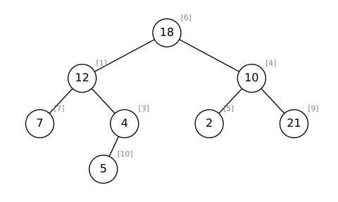
Reading off the pointers: \(6 \to (1, 4)\); \(1 \to (7, 3)\); \(3 \to (10, \text{NIL})\); \(4 \to (5, 9)\); indices 7, 10, 5, 9 are leaves. In preorder the keys are \(18, 12, 7, 4, 5, 10, 2, 21\). Indices 2 and 8 (keys 15 and 14) are unreachable from index 6, so they are not in the tree.
Give a recursive procedure that, given an \(n\)-node binary tree, prints the key of every node and runs in \(O(n)\) time.
Print the current node’s key, then recurse on its left and right subtrees (a preorder walk); call it as PRINT-TREE(T.root).
PRINT-TREE(x)
1  if x != NIL
2      print x.key
3      PRINT-TREE(x.left)
4      PRINT-TREE(x.right)
Correctness, by induction on the size of the subtree rooted at \(x\): for \(x = \text{NIL}\) nothing is printed; otherwise line 2 prints \(x\) and, by the inductive hypothesis, lines 3 and 4 print exactly the keys of the two subtrees, which together with \(x\) are the nodes of the subtree rooted at \(x\), each once.
Running time: each of the \(n\) nodes is the argument of exactly one call (the call from its parent, or the top call for the root), and each of the \(n+1\) NIL child pointers is the argument of exactly one call. Every call does \(O(1)\) work apart from its recursive calls, so the total is
\begin{equation*} (n + (n+1)) \cdot O(1) = O(n), \end{equation*}
as in Theorem 12.1 for INORDER-TREE-WALK.
Give a nonrecursive procedure that, given an \(n\)-node binary tree, prints the key of every node in \(O(n)\) time, using a stack as auxiliary data structure.
Keep a stack of roots of subtrees still to be printed: pop a node, print it, and push its non-NIL children (right first, so the output is in preorder).
PRINT-TREE-STACK(T)
1  let S be an empty stack of capacity n
2  if T.root != NIL
3      PUSH(S, T.root)
4  while not STACK-EMPTY(S)
5      x = POP(S)
6      print x.key
7      if x.right != NIL
8          PUSH(S, x.right)
9      if x.left != NIL
10         PUSH(S, x.left)
Loop invariant: at the start of each iteration of the while loop, the nodes already printed and the nodes of the subtrees rooted at the nodes in \(S\) together form the whole tree, each node occurring exactly once (the subtrees in \(S\) are disjoint and contain no printed node).
- Initialization: nothing is printed and \(S\) holds the root (or is empty for the empty tree).
- Maintenance: popping \(x\) and printing it removes the subtree of \(x\) from \(S\) and adds \(x\) to the printed set; pushing the non-NIL children puts back exactly the rest of that subtree, as two disjoint subtrees.
- Termination: when \(S\) is empty, the printed nodes are the whole tree, each printed once.
Running time: each node is pushed exactly once (by the invariant, a node enters \(S\) only when its parent is popped, or as the root) and hence popped once, so the loop runs \(n\) times; each iteration and each stack operation (Section 10.1) take \(O(1)\) time, and \(S\) never holds more than \(n\) nodes. The total is \(O(n)\).
An arbitrary rooted tree with \(n\) nodes is stored in the left-child, right-sibling representation (each node \(x\) has \(x.\mathit{left\text{-}child}\), pointing to its leftmost child, and \(x.\mathit{right\text{-}sibling}\), pointing to the sibling immediately to its right). Give an \(O(n)\)-time procedure that prints all the keys.
Walk along a sibling list, printing each node and recursing into its children through its left-child pointer; call PRINT-LCRS(T.root).
PRINT-LCRS(x)
1  while x != NIL
2      print x.key
3      PRINT-LCRS(x.left-child)
4      x = x.right-sibling
Correctness: for a node \(x\), let \(F(x)\) be the set of nodes in the subtrees rooted at \(x\) and at all siblings to the right of \(x\) (with \(F(\text{NIL}) = \emptyset\)). We claim PRINT-LCRS\((x)\) prints each node of \(F(x)\) exactly once; induct on \(|F(x)|\). If \(x = \text{NIL}\) nothing is printed. Otherwise
\begin{equation*} F(x) = \{x\} \,\cup\, F(x.\mathit{left\text{-}child}) \,\cup\, F(x.\mathit{right\text{-}sibling}), \end{equation*}
a disjoint union, since the children of \(x\) are \(x.\mathit{left\text{-}child}\) and its right siblings. The first iteration prints \(x\) and, by induction, line 3 prints \(F(x.\mathit{left\text{-}child})\); the remaining iterations do exactly what PRINT-LCRS\((x.\mathit{right\text{-}sibling})\) would do, which by induction prints \(F(x.\mathit{right\text{-}sibling})\). Since the root has no siblings, \(F(T.\mathit{root})\) is the whole tree.
Running time: every iteration of a while loop prints a distinct node, so there are exactly \(n\) iterations in total; each makes one recursive call, so there are at most \(n+1\) calls. Each iteration and each call cost \(O(1)\) apart from nested calls, giving \(O(n)\) in total.
Give a nonrecursive procedure that, given an \(n\)-node binary tree, prints the key of every node in \(O(n)\) time, using only constant extra space beyond the tree itself and without modifying the tree, not even temporarily.
Walk the tree along its edges using the parent pointers \(x.p\) of Figure 10.9, remembering only the previously visited node: whether we arrived at \(x\) from \(x.p\), from \(x.\mathit{left}\) or from \(x.\mathit{right}\) tells us where to go next, exactly as the recursion of Exercise 10.4-2 would.
PRINT-TREE-CONST(T)
1  prev = NIL
2  x = T.root
3  while x != NIL
4      if prev == x.p                 // arrived from the parent
5          print x.key
6          if x.left != NIL
7              next = x.left
8          elseif x.right != NIL
9              next = x.right
10         else next = x.p
11     elseif prev == x.left and x.right != NIL
12         next = x.right             // left subtree done
13     else next = x.p                // both subtrees done
14     prev = x
15     x = next
Correctness. Claim: if an iteration begins with \(x = y\) and \(\mathit{prev} = y.p\) for a node \(y\), then the loop prints the keys of the subtree rooted at \(y\) in preorder, each once, and later reaches an iteration with \(x = y.p\) and \(\mathit{prev} = y\), touching only nodes of that subtree in between. Induct on the subtree’s size. The first iteration prints \(y\) (line 4 holds). Then:
(i) \(y.\mathit{left} \ne \text{NIL}\): we move to \(y.\mathit{left}\) with \(\mathit{prev} = y\), so by induction the left subtree is printed and we return with \(x = y\), \(\mathit{prev} = y.\mathit{left}\). Line 4 fails (a child is not \(y.p\)), and line 11 sends us into \(y.\mathit{right}\) if it exists, whence by induction we return with \(\mathit{prev} = y.\mathit{right}\); now lines 4 and 11 fail and line 13 moves to \(y.p\).
(ii) \(y.\mathit{left} = \text{NIL} \ne y.\mathit{right}\): lines 8-9 enter the right subtree; on return \(\mathit{prev} = y.\mathit{right} \ne \text{NIL} = y.\mathit{left}\), so line 13 moves to \(y.p\).
(iii) \(y\) is a leaf: line 10 moves to \(y.p\).
In each case the output is \(y\) followed by the preorder of its left and then right subtree. The procedure starts with \(x = T.\mathit{root}\) and \(\mathit{prev} = \text{NIL} = T.\mathit{root}.p\), so it prints the whole tree and stops when \(x\) becomes \(T.\mathit{root}.p = \text{NIL}\) (for an empty tree the loop does not run).
Space and time: besides the tree, only the three pointers \(x\), \(\mathit{prev}\), \(\mathit{next}\) are stored, and no attribute is ever written. Each iteration costs \(O(1)\) and moves along one tree edge or from the root to NIL; by the claim each of the \(n-1\) edges is traversed once downward and once upward, so there are \(2(n-1)+1 = O(n)\) iterations.
The left-child, right-sibling representation of an arbitrary rooted tree stores three pointers per node: left-child, right-sibling and parent. With them, a node’s parent is found in constant time, and all of a node’s children are found in time linear in the number of children. Show how to store only two pointers and one boolean per node so that both the parent of a node and all of its children can be found in time linear in the number of children.
Keep \(x.\mathit{left\text{-}child}\), replace the other two pointers by a single pointer \(x.\mathit{next}\), and add a boolean \(x.\mathit{last}\): \(x.\mathit{last}\) is TRUE iff \(x\) is the rightmost child of its parent (or the root), and
\begin{equation*} x.\mathit{next} = \begin{cases} \text{the right sibling of } x & \text{if } x.\mathit{last} = \text{FALSE},\\ x.p & \text{if } x.\mathit{last} = \text{TRUE} \end{cases} \end{equation*}
(so the root has \(\mathit{last} = \text{TRUE}\), \(\mathit{next} = \text{NIL}\)). Each sibling list thus ends in a pointer back to the parent instead of NIL.
PARENT(x)
1  while x.last == FALSE
2      x = x.next
3  return x.next

CHILDREN(x)
1  y = x.left-child
2  while y != NIL
3      visit y
4      if y.last == TRUE
5          return
6      y = y.next
PARENT\((x)\) follows right-sibling pointers from \(x\) (by the definition of \(\mathit{next}\) on nodes with \(\mathit{last} = \text{FALSE}\)) until it reaches the rightmost child of \(x.p\), whose \(\mathit{next}\) is \(x.p\); it visits only children of \(x.p\), so it takes \(O(k)\) time where \(k\) is the number of children of \(x.p\) (the number of siblings of \(x\), itself included). CHILDREN\((x)\) starts at the leftmost child, follows right-sibling pointers, and stops at the rightmost child, recognised by its \(\mathit{last}\) flag, so it visits exactly the children of \(x\) in \(O(1 + \text{number of children})\) time.
Problems for Chapter 10
Comparisons among lists: consider four kinds of linked list: unsorted singly linked, sorted singly linked, unsorted doubly linked, and sorted doubly linked. For each kind, give the asymptotic worst-case running time of each of the dynamic-set operations SEARCH\((L,k)\), INSERT\((L,x)\), DELETE\((L,x)\), SUCCESSOR\((L,x)\), PREDECESSOR\((L,x)\), MINIMUM\((L)\) and MAXIMUM\((L)\), filling in a table whose rows are the operations and whose columns are the four list types.
With \(n\) elements, lists accessed through \(L.head\) only (as in Section 10.2, no tail pointer or sentinel), and SUCCESSOR/PREDECESSOR meaning the next larger/smaller key:
| operation | unsorted, singly | sorted, singly | unsorted, doubly | sorted, doubly |
|---|---|---|---|---|
| SEARCH\((L,k)\) | \(\Theta(n)\) | \(\Theta(n)\) | \(\Theta(n)\) | \(\Theta(n)\) |
| INSERT\((L,x)\) | \(\Theta(1)\) | \(\Theta(n)\) | \(\Theta(1)\) | \(\Theta(n)\) |
| DELETE\((L,x)\) | \(\Theta(n)\) | \(\Theta(n)\) | \(\Theta(1)\) | \(\Theta(1)\) |
| SUCCESSOR\((L,x)\) | \(\Theta(n)\) | \(\Theta(1)\) | \(\Theta(n)\) | \(\Theta(1)\) |
| PREDECESSOR\((L,x)\) | \(\Theta(n)\) | \(\Theta(n)\) | \(\Theta(n)\) | \(\Theta(1)\) |
| MINIMUM\((L)\) | \(\Theta(n)\) | \(\Theta(1)\) | \(\Theta(n)\) | \(\Theta(1)\) |
| MAXIMUM\((L)\) | \(\Theta(n)\) | \(\Theta(n)\) | \(\Theta(n)\) | \(\Theta(n)\) |
Justification, row by row:
- SEARCH: LIST-SEARCH walks from the head; sortedness only lets it stop early, and a key larger than all others (or absent) still costs \(n\) steps, since a linked list allows no random access.
- INSERT: an unsorted list takes \(x\) at the head (LIST-INSERT, \(O(1)\)); a sorted list must first walk to the position of \(x.key\), which is the tail when \(x.key\) is largest.
- DELETE: given the pointer \(x\), LIST-DELETE splices \(x\) out in \(O(1)\) using \(x.prev\); a singly linked list must scan from the head to find the predecessor node, \(\Theta(n)\) when \(x\) is last.
- SUCCESSOR: in a sorted list it is \(x.next\); in an unsorted list the next larger key can be anywhere, so every element must be examined.
- PREDECESSOR: in a sorted doubly linked list it is \(x.prev\); a sorted singly linked list must scan from the head for the node whose \(next\) is \(x\); an unsorted list again needs a full scan.
- MINIMUM: the head of a sorted list; a full scan otherwise.
- MAXIMUM: a full scan when unsorted; the last node of a sorted list, reached only by walking the whole list from the head.
Mergeable heaps using linked lists: a mergeable heap supports MAKE-HEAP (create an empty mergeable heap), INSERT, MINIMUM, EXTRACT-MIN and UNION. (Since it supports MINIMUM and EXTRACT-MIN it is a mergeable min-heap; with MAXIMUM and EXTRACT-MAX it would be a mergeable max-heap.) Show how to implement mergeable heaps with linked lists in each case below, making every operation as efficient as you can, and analyze each operation’s running time in terms of the sizes of the dynamic sets involved.
(a) The lists are sorted.
(b) The lists are unsorted.
(c) The lists are unsorted, and the dynamic sets passed to UNION are disjoint.
Write \(n\) for the size of the heap operated on and \(n_1,n_2\) for the sizes of the two heaps passed to UNION; an element is identified by its key, so a union of overlapping sets must keep one copy of each common key.
(a) Keep the keys in a singly linked list in increasing order: MAKE-HEAP, MINIMUM and EXTRACT-MIN take \(O(1)\), INSERT takes \(\Theta(n)\) and UNION takes \(\Theta(n_1+n_2)\). MAKE-HEAP sets \(H.head=\) NIL; MINIMUM returns \(H.head\); EXTRACT-MIN unlinks and returns \(H.head\); INSERT walks to the first node with a larger key and splices \(x\) in front of it, which costs \(\Theta(n)\) when \(x.key\) is the largest. UNION merges the two lists as in MERGE (Section 2.3.1), keeping one copy of an equal pair:
SORTED-UNION(H1, H2)
 1  let T be a dummy list node
 2  tail = T
 3  a = H1.head
 4  b = H2.head
 5  while a != NIL and b != NIL
 6      if a.key < b.key
 7          tail.next = a, a = a.next
 8      elseif b.key < a.key
 9          tail.next = b, b = b.next
10      else tail.next = a, a = a.next, b = b.next
11      tail = tail.next
12  if a != NIL
13      tail.next = a
14  else tail.next = b
15  H1.head = T.next
16  return H1
Loop invariant: at the start of each iteration of lines 5-11, the list from \(T.next\) to \(tail\) contains, in increasing order and without repeats, exactly the keys of \(H_1\) before \(a\) together with the keys of \(H_2\) before \(b\), and each of them is smaller than every key at or after \(a\) and \(b\).
- Initialization: the list is empty and nothing precedes \(a\) or \(b\).
- Maintenance: the node appended is the smaller of \(a.key\) and \(b.key\) (when they are equal, a single copy, with \(b\) skipped), so it is larger than everything already in the output and no larger than every key that remains; both lists are increasing.
- Termination: one list is used up, and the remainder of the other is increasing, has no repeats and lies entirely above the output, so lines 12-14 complete the sorted union.
Every iteration advances \(a\) or \(b\), so there are at most \(n_1+n_2\) iterations, each \(O(1)\); when the two lists interleave there are exactly \(n_1+n_2-1\), giving \(\Theta(n_1+n_2)\).
(b) Keep a circular, doubly linked list with a sentinel (Figure 10.4) plus a pointer \(H.min\) to the node with smallest key (NIL when empty). Then MAKE-HEAP, INSERT and MINIMUM take \(O(1)\), EXTRACT-MIN takes \(\Theta(n)\) and UNION takes \(\Theta(m\lg m)\), where \(m=n_1+n_2\).
- MAKE-HEAP creates the sentinel and sets \(H.min=\) NIL; INSERT puts \(x\) at the front (LIST-INSERT’) and sets \(H.min=x\) if \(H.min=\) NIL or \(x.key<H.min.key\); MINIMUM returns \(H.min\).
- EXTRACT-MIN splices out \(H.min\) in \(O(1)\) (LIST-DELETE’), then scans the remaining \(n-1\) nodes to set the new \(H.min\). The scan cannot be avoided: the remaining keys are unordered, and finding their minimum takes \(n-2\) comparisons (Section 9.1).
- UNION must discard the keys of \(H_2\) already in \(H_1\). Concatenate the lists in \(O(1)\) (as in part (c)), sort the resulting \(m\) nodes with merge sort in \(\Theta(m\lg m)\) (merge sort works on linked lists, since MERGE only scans forward), delete each node whose key equals its predecessor’s in one \(\Theta(m)\) pass, and set \(H.min\) to the first node.
(c) Use the structure of part (b): MAKE-HEAP, INSERT and MINIMUM stay \(O(1)\) and EXTRACT-MIN stays \(\Theta(n)\), but UNION is now \(O(1)\), because disjoint sets have no duplicates and the lists can simply be spliced:
DISJOINT-UNION(H1, H2)
1  if H2.nil.next != H2.nil
2      H1.nil.prev.next = H2.nil.next
3      H2.nil.next.prev = H1.nil.prev
4      H2.nil.prev.next = H1.nil
5      H1.nil.prev = H2.nil.prev
6      if H1.min == NIL or H2.min.key < H1.min.key
7          H1.min = H2.min
8  return H1
Lines 2-5 link the last node of \(H_1\) to the first node of \(H_2\) and the last node of \(H_2\) back to \(H_1\)’s sentinel, so \(H_1\) becomes a circular, doubly linked list of all \(n_1+n_2\) elements, and they are all distinct because the sets are disjoint. The minimum of the union is the smaller of the two minima, which lines 6-7 select. Each line takes constant time, so UNION runs in \(O(1)\).
Searching a sorted compact list: As in Exercise 10.3-4, an \(n\)-element linked list is stored compactly in positions \(1,\dots,n\) of the arrays. Assume all keys are distinct and the list is sorted, so \(key[i] < key[next[i]]\) for every \(i = 1,\dots,n\) with \(next[i] \ne \text{NIL}\), and a variable \(L\) holds the index of the head. The aim is to show that the following randomized procedure searches the list in \(O(\sqrt{n})\) expected time.
COMPACT-LIST-SEARCH(L, n, k)
 1  i = L
 2  while i != NIL and key[i] < k
 3      j = RANDOM(1, n)
 4      if key[i] < key[j] and key[j] <= k
 5          i = j
 6          if key[i] == k
 7              return i
 8      i = next[i]
 9  if i == NIL or key[i] > k
10      return NIL
11  else return i
Without lines 3-7 this is the ordinary scan of a sorted list, which stops when \(i\) runs off the end or \(key[i] \ge k\). Lines 3-7 try to jump ahead to a random slot \(j\); the jump is useful when \(key[i] < key[j] \le k\), and compactness guarantees that every \(j \in \{1,\dots,n\}\) is a list element. For the analysis consider the two-loop variant, with an extra parameter \(t\) bounding the first loop:
COMPACT-LIST-SEARCH'(L, n, k, t)
 1  i = L
 2  for q = 1 to t
 3      j = RANDOM(1, n)
 4      if key[i] < key[j] and key[j] <= k
 5          i = j
 6          if key[i] == k
 7              return i
 8  while i != NIL and key[i] < k
 9      i = next[i]
10  if i == NIL or key[i] > k
11      return NIL
12  else return i
Assume both procedures receive the same sequence of values from RANDOM(1, n).
(a) Suppose COMPACT-LIST-SEARCH(L, n, k) performs \(t\) iterations of its while loop (lines 2-8). Argue that COMPACT-LIST-SEARCH’(L, n, k, t) returns the same answer, and that its for and while loops together perform at least \(t\) iterations.
In COMPACT-LIST-SEARCH’(L, n, k, t), let \(X_t\) be the distance along the list (counted in next pointers) from position \(i\) to the desired key \(k\) after the \(t\) iterations of the for loop (lines 2-7).
(b) Argue that COMPACT-LIST-SEARCH’(L, n, k, t) runs in expected time \(O(t + \mathrm{E}[X_t])\).
(c) Show that \(\mathrm{E}[X_t] \le \sum_{r=1}^{n} (1 - r/n)^t\). (Hint: use equation (C.25).)
(d) Show that \(\sum_{r=0}^{n-1} r^t \le n^{t+1}/(t+1)\).
(e) Prove that \(\mathrm{E}[X_t] \le n/(t+1)\).
(f) Show that COMPACT-LIST-SEARCH’(L, n, k, t) runs in \(O(t + n/t)\) expected time.
(g) Conclude that COMPACT-LIST-SEARCH runs in \(O(\sqrt{n})\) expected time.
(h) Why is distinctness of the keys assumed? Argue that, when keys may repeat, random skips do not necessarily help asymptotically.
(a) Both return the correct answer, which (keys being distinct) is unique: the index holding \(k\), or NIL. Indeed a jump only goes to a \(j\) with \(key[j] \le k\), so a jump never passes the element holding \(k\), and line 7 returns only when \(key[i] = k\); after the jumps, each procedure finishes with the ordinary scan, which is correct from any start that is not past \(k\). For the iteration count, list order and key order coincide, so compare positions by key (with \(key[\text{NIL}] = +\infty\)); let \(i_q\), \(i^{\prime}_q\) be the positions of the two procedures after \(q\) iterations of their first loops, both using draw \(j_q\) in iteration \(q\). The domination invariant is
\begin{equation*} key[i^{\prime}_q] \le key[i_q] \qquad (0 \le q \le \min(t, T)), \end{equation*}
where \(T\) is the number of iterations of COMPACT-LIST-SEARCH. It holds at \(q = 0\) (\(i_0 = i^{\prime}_0 = L\)). For the inductive step, lines 4-5 send a position \(x\) to \(\phi(x) = \max(x, key[j_q])\) if \(key[j_q] \le k\), and leave it alone otherwise. Since \(\phi\) is monotone, \(key[i^{\prime}_{q+1}] = \phi(key[i^{\prime}_q]) \le \phi(key[i_q])\), and line 8 then moves COMPACT-LIST-SEARCH strictly further forward. Now suppose COMPACT-LIST-SEARCH takes \(t\) iterations. If COMPACT-LIST-SEARCH’ returns at line 7 in iteration \(q \le t\), then \(key[j_q] = k\). COMPACT-LIST-SEARCH is still running at iteration \(q\), so \(key[i^{\prime}_{q-1}] \le key[i_{q-1}] < k = key[j_q]\), which means it also jumps to \(j_q\) and returns there, giving \(q = t\). Otherwise all \(t\) iterations of the for loop are executed. Either way the total is at least \(t\).
(b) Each for-loop iteration costs \(O(1)\), and the while loop runs once for each next pointer followed, so it runs at most \(X_t + 1\) times. Here, when \(k\) is absent, \(X_t\) is measured to the last element with key less than \(k\), and \(X_t = 0\) if there is no such element or if the procedure has already returned. The cost is therefore \(O(t + X_t + 1) = O(t + X_t)\) for \(t \ge 1\), and taking expectations gives \(O(t + \mathrm{E}[X_t])\).
(c) Let \(p\) be the target of (b): the element holding \(k\), or else the last element with key less than \(k\). Every position \(i\) ever reached satisfies \(key[i] \le key[p]\) (jumps require \(key[j] \le k\), and a jump to \(k\) returns), except in the degenerate cases where \(X_t = 0\). Fix \(r \ge 1\). If \(p\) has fewer than \(r - 1\) predecessors then \(X_t < r\) surely; otherwise let \(S_r\) be the \(r\) elements at distances \(0, 1, \dots, r-1\) before \(p\). Each of them has key at most \(key[p] \le k\). If some draw \(j_q\) lands in \(S_r\), then after iteration \(q\) the position \(i\) is at \(j_q\) or beyond it, hence within distance \(r - 1\) of \(p\), and positions never move backward. So \(\{X_t \ge r\}\) is contained in the event that none of the \(t\) independent uniform draws lands in \(S_r\):
\begin{equation*} \Pr\{X_t \ge r\} \le (1 - r/n)^t . \end{equation*}
Since \(X_t \le n - 1\), equation (C.25) gives
\begin{equation*} \mathrm{E}[X_t] = \sum_{r=1}^{n} \Pr\{X_t \ge r\} \le \sum_{r=1}^{n} (1 - r/n)^t . \end{equation*}
(d) The function \(x \mapsto x^t\) is increasing on \([0, \infty)\), so the integral bound (A.11) gives
\begin{equation*} \sum_{r=0}^{n-1} r^t \le \int_0^n x^t \, dx = \frac{n^{t+1}}{t+1} . \end{equation*}
(e) Substitute \(s = n - r\) in (c) and then apply (d):
\begin{equation*} \begin{aligned} \mathrm{E}[X_t] &\le \sum_{r=1}^{n} \Bigl(\frac{n-r}{n}\Bigr)^t \\ &= \frac{1}{n^t} \sum_{s=0}^{n-1} s^t \\ &\le \frac{1}{n^t} \cdot \frac{n^{t+1}}{t+1} = \frac{n}{t+1} . \end{aligned} \end{equation*}
(f) By (b) and (e), the expected time is \(O(t + n/(t+1)) = O(t + n/t)\).
(g) Fix \(t = \lceil \sqrt{n} \rceil\) and let \(W_t\) be the number of while-loop iterations of COMPACT-LIST-SEARCH’(L, n, k, t). We claim \(T \le t + W_t\). If \(T \le t\) there is nothing to prove. Otherwise COMPACT-LIST-SEARCH’ did not return in its for loop (by (a), it would then return in the same iteration as COMPACT-LIST-SEARCH), and by the invariant of (a), \(i_t\) is at or beyond \(i^{\prime}_t\) and still has key less than \(k\). Every later iteration of COMPACT-LIST-SEARCH either returns or advances at least one step (line 8), and it stops at the same place where the while loop of COMPACT-LIST-SEARCH’ stops, which lies \(W_t\) steps beyond \(i^{\prime}_t\). Hence \(T - t \le W_t\). Using \(W_t \le X_t + 1\) from (b) and the bound from (e),
\begin{equation*} \begin{aligned} \mathrm{E}[T] &\le t + \mathrm{E}[X_t] + 1 \\ &\le \lceil \sqrt{n} \rceil + \frac{n}{\lceil \sqrt{n} \rceil + 1} + 1 = O(\sqrt{n}) , \end{aligned} \end{equation*}
and each iteration costs \(O(1)\), so COMPACT-LIST-SEARCH runs in \(O(\sqrt{n})\) expected time.
(h) The jump test \(key[i] < key[j]\) makes progress only by landing on a strictly larger key, so a long run of equal keys can be crossed only one step at a time. For example, take keys \(0, 0, \dots, 0, 1\) (\(n - 1\) zeros) in nondecreasing order, stored in any compact arrangement, and search for \(k = 1\). A jump succeeds only when \(j\) is the single element with key \(1\), which has probability \(1/n\) per iteration; otherwise \(i\) advances one step. So \(T = \min(G, n-1)\) with \(G\) geometric with parameter \(1/n\), and since \((1 - 1/n)^{n-1} \le 1/2\) for \(n \ge 2\),
\begin{equation*} \begin{aligned} \mathrm{E}[T] &= \sum_{q=1}^{n-1} \Bigl(1 - \frac{1}{n}\Bigr)^{q-1} \\ &= n\Bigl(1 - \bigl(1 - \tfrac{1}{n}\bigr)^{n-1}\Bigr) \ge \frac{n}{2} . \end{aligned} \end{equation*}
This is \(\Theta(n)\), no better asymptotically than the plain scan.
Chapter 11: Hash Tables
11.1 Direct-address tables
A dynamic set \(S\) is stored in a direct-address table \(T\) of length \(m\). Give a procedure that returns the maximum element of \(S\), and state its worst-case running time.
Scan \(T\) from slot \(m-1\) down to slot \(0\) and return the first non-NIL slot; the worst case is \(\Theta(m)\).
DIRECT-ADDRESS-MAXIMUM(T)
1  for k = T.length - 1 downto 0
2      if T[k] != NIL
3          return T[k]
4  return NIL              // S is empty
Since slot \(k\) holds the element with key \(k\), keys increase with the index, so the first non-NIL slot met when scanning downward holds the largest key; if no slot is non-NIL, \(S=\emptyset\). Each iteration costs \(O(1)\), and when \(S\) is empty (or contains only key \(0\)) all \(m\) slots are examined, so the worst case is \(\Theta(m)\).
A bit vector is an array of bits (each entry 0 or 1); one of length \(m\) needs far less space than an array of \(m\) pointers. Explain how a bit vector can represent a dynamic set of distinct elements that carry no satellite data, with every dictionary operation running in \(O(1)\) time.
Use a bit vector \(B[0\,..\,m-1]\) with \(B[k]=1\) exactly when key \(k\) is in the set; initially every bit is \(0\).
BIT-VECTOR-SEARCH(B, k)
1  return B[k] == 1

BIT-VECTOR-INSERT(B, k)
1  B[k] = 1

BIT-VECTOR-DELETE(B, k)
1  B[k] = 0
Since there is no satellite data, an element is identified with its key, so the invariant \(B[k]=1 \iff k\in S\) is all the set information there is; each procedure preserves it (INSERT adds \(k\), DELETE removes \(k\), distinctness means one bit per element suffices), and SEARCH reads it off. Each operation reads or writes one bit at a computable index (word \(\lfloor k/w\rfloor\), bit \(k \bmod w\) for word size \(w\)), so it takes \(O(1)\) time, and the structure uses \(m\) bits instead of \(m\) pointers.
Propose an implementation of a direct-address table in which several stored elements may share the same key and elements may carry satellite data. INSERT, DELETE and SEARCH must each run in \(O(1)\) time. Keep in mind that DELETE receives a pointer to the object being removed, not a key.
Let slot \(T[k]\) point to the head of a doubly linked list (Section 10.2) of all elements with key \(k\), or be NIL when there are none.
DA-SEARCH(T, k)
1  return T[k]            // head of the list of elements with key k

DA-INSERT(T, x)
1  x.next = T[x.key]
2  if T[x.key] != NIL
3      T[x.key].prev = x
4  T[x.key] = x
5  x.prev = NIL

DA-DELETE(T, x)
1  if x.prev != NIL
2      x.prev.next = x.next
3  else T[x.key] = x.next
4  if x.next != NIL
5      x.next.prev = x.prev
Invariant: for every \(k\), the list hanging from \(T[k]\) consists exactly of the stored elements with key \(k\). INSERT splices \(x\) in at the head of list \(x.key\) (this is LIST-INSERT of Section 10.2 with \(T[x.key]\) as the head), and DELETE unlinks \(x\) from list \(x.key\) using its own prev and next pointers (LIST-DELETE), so both preserve the invariant; SEARCH returns an element with key \(k\) (the head) or NIL if none exists, and also gives access to all of them. Each procedure does a constant number of pointer assignments with no traversal, because DELETE is handed \(x\) itself and the list is doubly linked, so all three run in \(O(1)\) time.
We want a dictionary implemented by direct addressing on a huge array \(T\). Initially the entries of \(T\) hold arbitrary garbage, and clearing the whole array is too expensive. Design a direct-address dictionary on this array such that each stored object occupies \(O(1)\) space, SEARCH, INSERT and DELETE each take \(O(1)\) time, and initializing the structure takes \(O(1)\) time. (Hint: keep an extra array, used like a stack whose size equals the number of keys currently stored, to decide whether a given entry of the huge array is valid.)
Keep an auxiliary array \(S\) used as a stack with counter \(S.top\) (initialized to \(0\), the only initialization), where \(S[1\,..\,S.top]\) holds pointers to the stored objects, and let \(T[k]\) be an index into \(S\); key \(k\) is present exactly when \(1\le T[k]\le S.top\) and \(S[T[k]].key=k\).
HUGE-SEARCH(T, S, k)
1  j = T[k]
2  if 1 <= j and j <= S.top and S[j].key == k
3      return S[j]
4  return NIL

HUGE-INSERT(T, S, x)    // x.key assumed absent
1  S.top = S.top + 1
2  S[S.top] = x
3  T[x.key] = S.top

HUGE-DELETE(T, S, x)
1  j = T[x.key]
2  y = S[S.top]          // move the top object into the hole
3  S[j] = y
4  T[y.key] = j
5  S.top = S.top - 1
Invariant: \(S[1\,..\,S.top]\) are exactly the stored objects, with distinct keys, and \(T[S[j].key]=j\) for every \(1\le j\le S.top\). It holds after initialization (\(S.top=0\), nothing stored), INSERT pushes \(x\) and links \(T[x.key]\) to it, and DELETE overwrites \(x\)’s stack cell with the top object \(y\), repoints \(T[y.key]\), and pops (when \(j=S.top\) this is just a pop); so it is maintained.
SEARCH is correct regardless of garbage:
\begin{equation*} \begin{aligned} k \text{ stored} &\Rightarrow k=S[j].key \text{ for some } j\le S.top,\ T[k]=j \Rightarrow \text{test passes},\\ \text{test passes} &\Rightarrow S[T[k]] \text{ is a stored object with key } k. \end{aligned} \end{equation*}
A garbage value in \(T[k]\) either falls outside \([1, S.top]\) or points to a valid cell whose object has a different key, so it is never mistaken for a hit; and the test reads \(S[j]\) only after checking \(j\le S.top\), so it never touches garbage in \(S\).
Every procedure does a constant number of array accesses, so SEARCH, INSERT, DELETE and initialization take \(O(1)\) time, and each stored object costs one stack cell plus one entry of \(T\), i.e. \(O(1)\) space.
11.2 Hash tables
A hash function \(h\) maps \(n\) distinct keys into a table \(T\) with \(m\) slots. Under simple uniform hashing, find the expected number of collisions, that is, the expected size of the set \(\{\{k,l\} : k \ne l \text{ and } h(k) = h(l)\}\).
The expected number of colliding pairs is \(\binom{n}{2}/m = n(n-1)/(2m)\).
For each unordered pair \(\{k,l\}\) of distinct keys let \(X_{kl} = \mathrm{I}\{h(k) = h(l)\}\). Simple uniform hashing gives \(\Pr\{h(k) = h(l)\} = 1/m\), so \(\mathrm{E}[X_{kl}] = 1/m\) by Lemma 5.1, and by linearity of expectation
\begin{equation*} \begin{aligned} \mathrm{E}\Bigl[\sum_{\{k,l\}} X_{kl}\Bigr] &= \sum_{\{k,l\}} \frac{1}{m} = \binom{n}{2}\frac{1}{m} = \frac{n(n-1)}{2m}. \end{aligned} \end{equation*}
Show the result of inserting the keys \(5, 28, 19, 15, 20, 33, 12, 17, 10\), in that order, into a hash table with \(9\) slots that resolves collisions by chaining, using the hash function \(h(k) = k \bmod 9\).
CHAINED-HASH-INSERT puts each new key at the head of its list, so the hash values \(h(5)=5\), \(h(28)=1\), \(h(19)=1\), \(h(15)=6\), \(h(20)=2\), \(h(33)=6\), \(h(12)=3\), \(h(17)=8\), \(h(10)=1\) produce the final table below (each list written head first).
| slot | chain |
|---|---|
| 0 | NIL |
| 1 | 10, 19, 28 |
| 2 | 20 |
| 3 | 12 |
| 4 | NIL |
| 5 | 5 |
| 6 | 33, 15 |
| 7 | NIL |
| 8 | 17 |
Professor Marley proposes keeping every chain of a chained hash table in sorted order, hoping for large speedups. How does this change the running times of successful searches, unsuccessful searches, insertions, and deletions?
There is no asymptotic gain: both kinds of search remain \(\Theta(1+\alpha)\) expected, insertion gets worse (from \(O(1)\) worst case to \(\Theta(1+\alpha)\) expected), and deletion stays \(O(1)\).
(i) Successful search. Searching for \(x\) scans its list up to \(x\), examining \(1\) plus the number of keys \(y < x\) in the same list. Averaging over the \(n\) keys \(x\), each colliding pair \(\{x,y\}\) is counted exactly once (for its larger key), so by Exercise 11.2-1 the expected number of elements examined is
\begin{equation*} 1 + \frac{1}{n}\cdot\frac{n(n-1)}{2m} = 1 + \frac{\alpha}{2} - \frac{\alpha}{2n}, \end{equation*}
exactly the count in the proof of Theorem 11.2. The time is still \(\Theta(1+\alpha)\).
(ii) Unsuccessful search. The scan of list \(T[h(k)]\) can stop at the first key larger than \(k\), but when \(k\) exceeds every key in the list the whole list is still read. The time is at most that of Theorem 11.1, \(\Theta(1+\alpha)\), and for such keys no better; at best the constant shrinks.
(iii) Insertion. The new key can no longer go at the head; we must scan the list to find its position, which costs as much as an unsuccessful search, \(\Theta(1+\alpha)\) expected, instead of the \(O(1)\) worst case of CHAINED-HASH-INSERT.
(iv) Deletion. Given a pointer to the element in a doubly linked list, splicing it out is \(O(1)\) worst case and removing an element keeps the list sorted, so nothing changes.
Explain how to allocate and free storage for elements inside the hash table itself, by threading all unused slots onto a free list. Each slot holds a flag together with either one element and one pointer, or two pointers. Every dictionary operation and every free-list operation must take \(O(1)\) expected time. Must the free list be doubly linked, or is a singly linked free list enough?
Keep the chain of slot \(j\) inside the table with its head stored in slot \(j\) itself, keep the free slots on a doubly linked free list (a free slot’s two pointers are its prev and next on that list), and evict any element that occupies another chain’s home slot; the free list must be doubly linked.
A used slot (flag USED) holds an element \(x\) and a pointer \(x.next\) to the next slot of its chain. The invariant is: chain \(j\) is nonempty if and only if slot \(j\) is used by a key \(k\) with \(h(k) = j\), and then that key heads chain \(j\). Allocation pops the head of the free list; freeing a slot pushes it onto the head; both are \(O(1)\).
Search for \(k\): if slot \(h(k)\) is free or holds a key whose hash is not \(h(k)\), the chain is empty; otherwise follow next pointers from slot \(h(k)\). Insertion:
HASH-INSERT(T, k)
 1  j = h(k)
 2  if T[j] is free
 3      unlink slot j from the free list   // needs prev pointer
 4      T[j].key = k;  T[j].next = NIL
 5  elseif h(T[j].key) == j                // slot j heads chain j
 6      i = ALLOCATE-SLOT()
 7      T[i].key = k;  T[i].next = T[j].next;  T[j].next = i
 8  else y = T[j].key                     // y belongs to chain h(y)
 9      i = ALLOCATE-SLOT()
10      T[i].key = y;  T[i].next = T[j].next
11      p = h(y)
12      while T[p].next != j
13          p = T[p].next
14      T[p].next = i                      // y now lives in slot i
15      T[j].key = k;  T[j].next = NIL
Deletion of the element in slot \(i\) with \(j = h(T[i].key)\): if \(i = j\) and \(T[i].next = q \ne\) NIL, copy the element in slot \(q\) (with its next pointer) into slot \(i\) and free slot \(q\); if \(i = j\) and the chain has one element, free slot \(i\); if \(i \ne j\), walk chain \(j\) from slot \(j\) to the predecessor \(p\) of \(i\), set \(T[p].next = T[i].next\), and free slot \(i\). Each case preserves the invariant (Check!), so search, insertion and deletion are correct.
Running time: apart from \(O(1)\) pointer work, each operation walks at most one chain, chain \(h(k)\) or chain \(h(y)\), whose length is the number of keys hashing to that slot. Under simple uniform hashing that is \(O(1+\alpha)\) expected (as in Theorems 11.1 and 11.2), and \(\alpha = n/m \le 1\) because every element occupies a slot, so all operations take \(O(1)\) expected time.
Doubly linked is needed: line 3 removes the particular slot \(j\), which can sit anywhere on the free list. With only a successor pointer, finding the predecessor of slot \(j\) on the free list could take \(\Theta(m)\) time; the prev pointer makes the unlinking \(O(1)\), and a free slot has room for both pointers.
A set of \(n\) keys is stored in a hash table with \(m\) slots, the keys coming from a universe \(U\) with \(|U| > nm\). Show that some \(n\)-element subset of \(U\) consists of keys that all hash to one slot, so that searching with chaining takes \(\Theta(n)\) time in the worst case.
By the pigeonhole principle some slot receives at least \(n\) keys of \(U\). Write \(U_j = \{k \in U : h(k) = j\}\). If \(|U_j| \le n-1\) for every \(j\), then
\begin{equation*} |U| = \sum_{j=0}^{m-1} |U_j| \le m(n-1) < nm, \end{equation*}
a contradiction. So some \(|U_j| \ge n\); let \(S\) be any \(n\) keys of \(U_j\). If the stored set is \(S\), all \(n\) keys sit in the single list \(T[j]\), and searching for the key at the tail of that list (or unsuccessfully for another key of \(U_j\)) examines all \(n\) elements, which is \(\Omega(n)\). Since no list can hold more than \(n\) elements, every search is \(O(n)\), so the worst case is \(\Theta(n)\).
A hash table with \(m\) slots holds \(n \ge 1\) keys, with collisions resolved by chaining, and the length of every chain is known, including the length \(L\) of the longest one. Give a procedure that returns a key chosen uniformly at random from the keys in the table, in expected time \(O(L \cdot (1 + 1/\alpha))\).
Use rejection sampling on an \(m \times L\) grid: pick a slot \(j\) and a position \(i \in \{1,\dots,L\}\) uniformly and independently, accept if chain \(j\) has at least \(i\) elements (and then walk to its \(i\)-th element), and otherwise retry.
RANDOM-KEY(T)
1  repeat
2      j = RANDOM(0, m - 1)
3      i = RANDOM(1, L)
4  until i <= length of chain T[j]
5  x = T[j].head
6  for t = 1 to i - 1
7      x = x.next
8  return x.key
Correctness: let \(n_j\) be the length of chain \(j\). Each of the \(mL\) pairs \((j,i)\) is equally likely in a trial, and the accepted pairs are in bijection with the \(n\) keys (pair \((j,i)\) with \(i \le n_j\) names the \(i\)-th key of chain \(j\)). So a trial accepts with probability
\begin{equation*} p = \sum_{j=0}^{m-1} \frac{n_j}{mL} = \frac{n}{mL} = \frac{\alpha}{L}, \end{equation*}
and, given acceptance, each key is the one named with probability \((1/(mL))/p = 1/n\). Trials are independent, so the returned key is uniform.
Running time: each trial costs \(O(1)\), since the chain lengths are known. The number of trials is geometric with success probability \(p\), so its expectation is \(1/p = L/\alpha\) (equation (C.32)). The final walk takes \(i - 1 < L\) steps. The expected total is
\begin{equation*} O\Bigl(\frac{L}{\alpha} + L\Bigr) = O\bigl(L \cdot (1 + 1/\alpha)\bigr). \end{equation*}
11.3 Hash functions
We must search a linked list of \(n\) elements, where each element stores a key \(k\) (a long character string) together with its hash value \(h(k)\). How can the stored hash values be exploited when searching the list for the element whose key equals a given key?
Compute \(h(k)\) for the search key \(k\) once, then while walking the list compare the stored hash value \(h(x.key)\) with \(h(k)\) first, and perform the expensive string comparison \(x.key = k\) only when the two hash values agree.
LIST-SEARCH-HASHED(L, k)
1  hk = h(k)
2  x = L.head
3  while x != NIL
4      if x.hash == hk and x.key == k
5          return x
6      x = x.next
7  return NIL
Since \(x.key = k\) implies \(h(x.key) = h(k)\), the hash test never rejects the sought element, so the result is exactly that of LIST-SEARCH. With key length \(L\) and \(c\) the number of elements whose stored hash equals \(h(k)\), the cost is
\begin{equation*} O(L + n + cL) \end{equation*}
instead of up to \(O(nL)\) for a string comparison at every element; with a good hash function into a large range, \(c\) is essentially the number of elements with key \(k\), giving \(O(n + L)\).
A string of \(r\) characters is hashed into \(m\) slots by reading it as a radix-128 number and applying the division method. The modulus \(m\) fits in one 32-bit word, but the radix-128 number occupies many words. Show how to compute the division-method hash value of the string while using only a constant number of words of storage beyond the string itself.
Evaluate the radix-128 number by Horner’s rule, reducing modulo \(m\) after every step. Writing the string as \(c_{r-1} c_{r-2} \cdots c_0\) (most significant character first), so that \(k = \sum_{i=0}^{r-1} c_i 128^i\):
STRING-HASH(c, r, m)
1  h = 0
2  for i = r - 1 downto 0
3      h = (128 * h + c[i]) mod m
4  return h
Correctness. Let \(k_i = \sum_{j=i}^{r-1} c_j 128^{\,j-i}\) be the number formed by the leading characters \(c_{r-1}\cdots c_i\). Loop invariant: at the start of the iteration for index \(i\), \(h = k_{i+1} \bmod m\) (with \(k_r = 0\)). Initially \(h = 0 = k_r \bmod m\). Maintenance: since \(k_i = 128\,k_{i+1} + c_i\) and \(h \equiv k_{i+1} \pmod m\),
\begin{equation*} (128h + c_i) \bmod m = (128\,k_{i+1} + c_i) \bmod m = k_i \bmod m . \end{equation*}
At termination (\(i = -1\)), \(h = k_0 \bmod m = k \bmod m\).
Space: \(0 \le h < m < 2^{32}\) and \(c_i < 128\), so \(128h + c_i < 128m + 128 \le 2^{39}\) fits in two 32-bit words; besides the string we store only \(h\), \(i\), \(m\) and this intermediate value, \(O(1)\) words, and the time is \(\Theta( r)\).
Consider the division-method variant \(h(k) = k \bmod m\) with \(m = 2^p - 1\), where the key \(k\) is a character string read as a number in radix \(2^p\). Prove that whenever string \(x\) is obtained from string \(y\) by permuting its characters, \(h(x) = h(y)\). Describe an application in which this property of a hash function would be undesirable.
Since \(2^p \equiv 1 \pmod{2^p - 1}\), the hash of a string is just the sum of its characters modulo \(m\), which no permutation changes. Indeed, if \(x = x_{r-1}\cdots x_0\) with character values \(0 \le x_i < 2^p\), then
\begin{equation*} h(x) = \Bigl(\sum_{i=0}^{r-1} x_i (2^p)^i\Bigr) \bmod m = \Bigl(\sum_{i=0}^{r-1} x_i \cdot 1^i\Bigr) \bmod m = \Bigl(\sum_{i=0}^{r-1} x_i\Bigr) \bmod m . \end{equation*}
If \(x_i = y_{\pi(i)}\) for a permutation \(\pi\) of \(\{0,\dots,r-1\}\), then \(\sum_i x_i = \sum_i y_{\pi(i)} = \sum_i y_i\), so \(h(x) = h(y)\).
Application where this hurts: a compiler’s symbol table or a dictionary of English words, where anagrams such as stop, pots, tops, spot, post, opts all land in the same slot, or a table of DNA \(k\)-mers over ACGT, where every \(k\)-mer with the same base composition collides; the chains degrade to long lists and searches to linear time.
A hash table has \(m = 1000\) slots and uses the multiplication-method hash function \(h(k) = \lfloor m\,(kA \bmod 1) \rfloor\) with \(A = (\sqrt5 - 1)/2\). Find the slots to which the keys 61, 62, 63, 64 and 65 hash.
The keys map to slots \(700, 318, 936, 554, 172\) respectively. With \(A = 0.6180339887\ldots\):
| \(k\) | \(kA\) | \(kA \bmod 1\) | \(h(k)\) |
|---|---|---|---|
| 61 | 37.70007331… | 0.70007331… | 700 |
| 62 | 38.31810730… | 0.31810730… | 318 |
| 63 | 38.93614129… | 0.93614129… | 936 |
| 64 | 39.55417528… | 0.55417528… | 554 |
| 65 | 40.17220927… | 0.17220927… | 172 |
A family \(\mathcal H\) of hash functions from a finite set \(U\) to a finite set \(B\) is called \(\epsilon\)-universal if every pair of distinct keys \(k, l \in U\) satisfies
\begin{equation*} \Pr\{h(k) = h(l)\} \le \epsilon , \end{equation*}
the probability being over a uniformly random choice of \(h\) from \(\mathcal H\). Prove that every \(\epsilon\)-universal family satisfies
\begin{equation*} \epsilon \ge \frac{1}{|B|} - \frac{1}{|U|} . \end{equation*}
Averaging the collision probability over all pairs gives at least \(\frac{|U|/|B| - 1}{|U| - 1} \ge \frac{1}{|B|} - \frac{1}{|U|}\) when \(|U| \ge |B|\); otherwise the bound is negative. Write \(u = |U| \ge 2\) (for \(u = 1\) there are no pairs and the condition is vacuous) and \(b = |B|\).
If \(u < b\) the right side is negative and \(\epsilon \ge \Pr\{\cdot\} \ge 0\) suffices. Let \(u \ge b\). Fix \(h \in \mathcal H\) and let \(u_j = |h^{-1}(j)|\) for \(j \in B\), so \(\sum_j u_j = u\). The number \(C(h)\) of unordered pairs \(\{k,l\}\), \(k \ne l\), with \(h(k) = h(l)\) satisfies, by the Cauchy-Schwarz inequality \(\sum_j u_j^2 \ge (\sum_j u_j)^2/b\),
\begin{equation*} C(h) = \sum_{j \in B} \binom{u_j}{2} = \frac12\Bigl(\sum_j u_j^2 - u\Bigr) \ge \frac12\Bigl(\frac{u^2}{b} - u\Bigr). \end{equation*}
Summing \(\Pr\{h(k)=h(l)\} \le \epsilon\) over all \(\binom u2\) pairs and using linearity of expectation,
\begin{equation*} \begin{aligned} \binom u2 \epsilon &\ge \sum_{\{k,l\}} \Pr\{h(k)=h(l)\} = \mathrm E[C(h)] \ge \frac{u}{2}\Bigl(\frac{u}{b} - 1\Bigr),\\ \epsilon &\ge \frac{u/b - 1}{u - 1} = \frac{u - b}{b(u-1)} \ge \frac{u - b}{bu} = \frac1b - \frac1u , \end{aligned} \end{equation*}
the last inequality because \(u - b \ge 0\) and \(u - 1 < u\).
Let \(p\) be prime, let \(U\) be the set of \(n\)-tuples with entries in \(\mathbb Z_p\), and let \(B = \mathbb Z_p\). For each \(b \in \mathbb Z_p\) define \(h_b : U \to B\) on an input \(\langle a_0, a_1, \dots, a_{n-1}\rangle\) by
\begin{equation*} h_b(\langle a_0, a_1, \dots, a_{n-1}\rangle) = \Bigl(\sum_{j=0}^{n-1} a_j b^j\Bigr) \bmod p , \end{equation*}
and set \(\mathcal H = \{h_b : b \in \mathbb Z_p\}\). Show that \(\mathcal H\) is \(((n-1)/p)\)-universal in the sense of Exercise 11.3-5. (Hint: use Exercise 31.4-4.)
Two distinct tuples collide under \(h_b\) exactly when \(b\) is a zero of a nonzero polynomial of degree at most \(n-1\) over \(\mathbb Z_p\), and such a polynomial has at most \(n-1\) zeros. Precisely, let \(a = \langle a_0,\dots,a_{n-1}\rangle \ne a^{\prime} = \langle a^{\prime}_0,\dots,a^{\prime}_{n-1}\rangle\) and put
\begin{equation*} f(x) = \sum_{j=0}^{n-1} (a_j - a^{\prime}_j)\, x^j \pmod p , \end{equation*}
whose coefficients are not all zero modulo \(p\), so \(f\) is a nonzero polynomial of some degree \(t \le n-1\). Then
\begin{equation*} h_b(a) = h_b(a^{\prime}) \iff \sum_{j} a_j b^j \equiv \sum_j a^{\prime}_j b^j \pmod p \iff f(b) \equiv 0 \pmod p . \end{equation*}
By Exercise 31.4-4 (\(p\) prime, \(f\) of degree \(t\)), \(f\) has at most \(t \le n-1\) distinct zeros in \(\mathbb Z_p\) (if \(t = 0\), \(f\) is a nonzero constant and has none). For \(n \ge 2\) the functions \(h_b\) are pairwise distinct (\(h_b(\langle 0,1,0,\dots,0\rangle) = b\)), so drawing \(h_b\) uniformly from \(\mathcal H\) means drawing \(b\) uniformly from \(\mathbb Z_p\) (for \(n = 1\) distinct tuples never collide, as \(f\) is a nonzero constant), and
\begin{equation*} \Pr\{h_b(a) = h_b(a^{\prime})\} = \frac{|\{b \in \mathbb Z_p : f(b) \equiv 0\}|}{p} \le \frac{n-1}{p} , \end{equation*}
so \(\mathcal H\) is \(((n-1)/p)\)-universal.
11.4 Open addressing
Insert the keys \(10, 22, 31, 4, 15, 28, 17, 88, 59\), in this order, into an open-address hash table of length \(m = 11\) with auxiliary hash function \(h^{\prime}(k) = k\). Show the resulting table for each of three probing schemes: linear probing; quadratic probing with \(c_1 = 1\) and \(c_2 = 3\); and double hashing with \(h_1(k) = k\) and \(h_2(k) = 1 + (k \bmod (m-1))\).
The final tables are (empty slots marked \(-\)):
| slot | 0 | 1 | 2 | 3 | 4 | 5 | 6 | 7 | 8 | 9 | 10 |
|---|---|---|---|---|---|---|---|---|---|---|---|
| linear | 22 | 88 | - | - | 4 | 15 | 28 | 17 | 59 | 31 | 10 |
| quadratic | 22 | - | 88 | 17 | 4 | - | 28 | 59 | 15 | 31 | 10 |
| double | 22 | - | 59 | 17 | 4 | 15 | 28 | 88 | - | 31 | 10 |
The keys \(10, 22, 31, 4, 28\) land at their home slots \(k \bmod 11 = 10, 0, 9, 4, 6\) in every scheme. The colliding keys follow these probe sequences (the last slot listed is where the key is stored):
Linear, \(h(k,i) = (k+i) \bmod 11\): \(15\): \(4, 5\); \(17\): \(6, 7\); \(88\): \(0, 1\); \(59\): \(4, 5, 6, 7, 8\).
Quadratic, \(h(k,i) = (k + i + 3i^2) \bmod 11\): \(15\): \(4, 8\); \(17\): \(6, 10, 9, 3\); \(88\): \(0, 4, 3, 8, 8, 3, 4, 0, 2\) (nine probes); \(59\): \(4, 8, 7\).
Double hashing, \(h(k,i) = (k + i(1 + k \bmod 10)) \bmod 11\), with step \(h_2(15) = 6\), \(h_2(17) = 8\), \(h_2(88) = 9\), \(h_2(59) = 10\): \(15\): \(4, 10, 5\); \(17\): \(6, 3\); \(88\): \(0, 9, 7\); \(59\): \(4, 3, 2\).
Following the outline in Section 11.4, give pseudocode for HASH-DELETE in an open-address table (a deleted key’s slot is overwritten with the special marker DELETED rather than NIL), and modify HASH-INSERT so that it handles DELETED slots.
HASH-DELETE searches for \(k\) along its probe sequence exactly as HASH-SEARCH does and overwrites the slot with DELETED; HASH-INSERT stores the key in the first slot that is NIL or DELETED. HASH-SEARCH is unchanged (it skips DELETED slots because DELETED is neither \(k\) nor NIL).
HASH-INSERT(T, k)
1  i = 0
2  repeat
3      j = h(k, i)
4      if T[j] == NIL or T[j] == DELETED
5          T[j] = k
6          return j
7      else i = i + 1
8  until i == m
9  error "hash table overflow"

HASH-DELETE(T, k)
1  i = 0
2  repeat
3      j = h(k, i)
4      if T[j] == k
5          T[j] = DELETED
6          return j
7      i = i + 1
8  until T[j] == NIL or i == m
9  return NIL                  // k was not in the table
Correctness rests on the invariant: for every key \(k\) stored in the table, if \(k\) sits in slot \(h(k,q)\), then none of \(h(k,0), \dots, h(k,q-1)\) is NIL. Initially the table is all NIL and holds no key. Maintenance: HASH-INSERT puts \(k\) at the first probe \(h(k,q)\) that is NIL or DELETED, so every earlier probe holds a key, which is non-NIL. The only slot changes are NIL \(\to\) key, DELETED \(\to\) key and key \(\to\) DELETED, so a slot that is non-NIL never becomes NIL again, and the invariant holds for keys already stored. Consequence: a search for a stored \(k\) (in HASH-SEARCH or lines 2-8 of HASH-DELETE) cannot stop at a NIL before reaching \(h(k,q)\), so it finds \(k\). If \(k\) is absent, line 4 of HASH-DELETE never matches and it returns NIL after hitting a NIL slot or making \(m\) probes. (As in the text, HASH-INSERT assumes \(k\) is not already present.)
For an open-address hash table under the uniform hashing assumption, give upper bounds on the expected number of probes in an unsuccessful search and in a successful search, first for load factor \(\alpha = 3/4\) and then for \(\alpha = 7/8\).
By Theorem 11.6 the unsuccessful bound is \(1/(1-\alpha)\), and by Theorem 11.8 the successful bound is \(\frac{1}{\alpha}\ln\frac{1}{1-\alpha}\) (both apply since \(\alpha < 1\)):
\begin{equation*} \begin{aligned} \alpha = 3/4:&\quad \frac{1}{1-3/4} = 4, &\quad \frac{4}{3}\ln 4 &\approx 1.848,\\ \alpha = 7/8:&\quad \frac{1}{1-7/8} = 8, &\quad \frac{8}{7}\ln 8 &\approx 2.377. \end{aligned} \end{equation*}
Double hashing uses \(h(k,i) = (h_1(k) + i\,h_2(k)) \bmod m\). Prove that if \(d = \gcd(m, h_2(k)) \ge 1\) for a key \(k\), then an unsuccessful search for \(k\) examines a \(1/d\) fraction of the table before it comes back to slot \(h_1(k)\). Deduce that when \(d = 1\) (that is, \(m\) and \(h_2(k)\) are relatively prime) the search may examine every slot. (Hint: Chapter 31.)
The probe sequence of \(k\) has period exactly \(m/d\) and its first \(m/d\) entries are distinct, so the search sees exactly \(m/d\) slots, a \(1/d\) fraction of the table, before returning to \(h_1(k)\). Write \(s = h_2(k)\), so \(s = d s^{\prime}\) and \(m = d m^{\prime}\) with \(\gcd(m^{\prime}, s^{\prime}) = 1\). For \(0 \le i^{\prime} < i\),
\begin{equation*} \begin{aligned} h(k,i) = h(k,i^{\prime}) &\iff m \mid (i - i^{\prime})s \iff d m^{\prime} \mid d s^{\prime}(i - i^{\prime})\\ &\iff m^{\prime} \mid s^{\prime}(i - i^{\prime}) \iff m^{\prime} \mid (i - i^{\prime}), \end{aligned} \end{equation*}
where the last step is Corollary 31.5 (applicable since \(\gcd(s^{\prime}, m^{\prime}) = 1\)). Hence \(h(k,0), \dots, h(k,m^{\prime}-1)\) are \(m^{\prime} = m/d\) distinct slots and \(h(k,m^{\prime}) = h(k,0) = h_1(k)\). An unsuccessful search that has not met an empty slot therefore probes exactly these \(m/d\) slots before it returns to \(h_1(k)\). When \(d = 1\) this is all \(m\) slots, so the probe sequence is a permutation of the table and the search may examine every slot.
Consider an open-address hash table with load factor \(\alpha\). Using the upper bounds of Theorems 11.6 and 11.8 as the expected numbers of probes, find the nonzero \(\alpha\) for which the expected probe count of an unsuccessful search is twice that of a successful search.
The unique such value is \(\alpha \approx 0.7153\), the root of \(1 - x + 2x\ln x = 0\) with \(x = 1 - \alpha\). Theorems 11.6 and 11.8 make the condition
\begin{equation*} \begin{aligned} \frac{1}{1-\alpha} = \frac{2}{\alpha}\ln\frac{1}{1-\alpha} &\iff \alpha = -2(1-\alpha)\ln(1-\alpha)\\ &\iff \varphi(x) := 1 - x + 2x\ln x = 0 . \end{aligned} \end{equation*}
Here \(\varphi^{\prime}(x) = 1 + 2\ln x\), so \(\varphi\) decreases on \((0, e^{-1/2})\) and increases on \((e^{-1/2}, 1)\). Since \(\varphi(1) = 0\) (this is \(\alpha = 0\), which is excluded), \(\varphi < 0\) on \([e^{-1/2}, 1)\). Since \(\varphi(0^+) = 1 > 0\), there is exactly one root in \((0, e^{-1/2})\). Numerically, \(x \approx 0.28467\), so
\begin{equation*} \alpha \approx 0.71533, \qquad \frac{1}{1-\alpha} \approx 3.513 = 2 \times 1.756 . \end{equation*}
11.5 Perfect hashing
Insert \(n\) keys into an open-addressed hash table with \(m\) slots under the uniform hashing assumption, and let \(p(n,m)\) denote the probability that the insertions produce no collision at all. Prove that \(p(n,m) \le e^{-n(n-1)/2m}\) (hint: use equation (3.12)). Then explain why the probability of avoiding every collision falls off rapidly toward zero once \(n\) is larger than \(\sqrt{m}\).
We have \(p(n,m) = \prod_{i=0}^{n-1}(1 - i/m)\), and each factor is at most \(e^{-i/m}\).
No collision occurs exactly when every key’s first probe lands in an empty slot. Under uniform hashing each key’s first probe is uniform over the \(m\) slots, independently of the other keys, so given that the first \(i\) keys occupy \(i\) distinct slots, the \((i+1)\)st avoids a collision with probability \((m-i)/m\). Multiplying and applying \(1 + x \le e^x\) (equation (3.12)) with \(x = -i/m\) gives
\begin{equation*} \begin{aligned} p(n,m) &= \prod_{i=0}^{n-1} \frac{m-i}{m} = \prod_{i=0}^{n-1}\Bigl(1 - \frac{i}{m}\Bigr) \\ &\le \prod_{i=0}^{n-1} e^{-i/m} = \exp\Bigl(-\frac{1}{m}\sum_{i=0}^{n-1} i\Bigr) \\ &= e^{-n(n-1)/2m}. \end{aligned} \end{equation*}
The factorwise bound is valid because every factor is nonnegative (for \(n > m\) the factor \(i = m\) is \(0\), so \(p(n,m) = 0\)).
If \(n \ge c\sqrt{m} + 1\) with \(c > 0\), then \(n(n-1) \ge c^2 m\), so
\begin{equation*} p(n,m) \le e^{-c^2/2}, \end{equation*}
which decays like a Gaussian in \(c\): \(c = 3\) gives \(p < 0.012\) and \(c = 5\) gives \(p < 4 \cdot 10^{-6}\). Hence once \(n\) exceeds \(\sqrt{m}\) by a modest constant factor, avoiding all collisions becomes vanishingly unlikely.
Problems for Chapter 11
Longest-probe bound for hashing: An open-address hash table of size \(m\) is used to store \(n \le m/2\) items.
(a) Assuming uniform hashing, show that for each \(i = 1, 2, \ldots, n\), the probability that the \(i\)th insertion needs strictly more than \(k\) probes is at most \(2^{-k}\).
(b) Show that for each \(i = 1, 2, \ldots, n\), the probability that the \(i\)th insertion needs more than \(2\lg n\) probes is \(O(1/n^2)\).
Let \(X_i\) be the number of probes used by the \(i\)th insertion, so part (b) says \(\Pr\{X_i > 2\lg n\} = O(1/n^2)\), and let \(X = \max_{1 \le i \le n} X_i\) be the largest number of probes used by any of the \(n\) insertions.
(c) Show that \(\Pr\{X > 2\lg n\} = O(1/n)\).
(d) Show that the expected length \(\mathrm{E}[X]\) of the longest probe sequence is \(O(\lg n)\).
(a) The \(i\)th insertion needs more than \(k\) probes exactly when its first \(k\) probes all land on occupied slots. When it starts, \(i - 1 < n \le m/2\) slots are occupied, and under uniform hashing the probe sequence is a uniformly random permutation of the \(m\) slots. So for \(k \le i-1\) (for larger \(k\) the probability is \(0\))
\begin{equation*} \begin{aligned} \Pr\{X_i > k\} &= \prod_{j=0}^{k-1} \frac{i-1-j}{m-j} \le \left(\frac{i-1}{m}\right)^{k} \\ &\le \left(\frac{1}{2}\right)^{k} = 2^{-k}, \end{aligned} \end{equation*}
using \((i-1-j)/(m-j) \le (i-1)/m\) for \(0 \le j < m\) (this rearranges to \(j(i-1) \le jm\)).
(b) The number of probes is an integer, so more than \(2\lg n\) probes means more than \(k = \lfloor 2\lg n \rfloor\) probes, and by (a)
\begin{equation*} \begin{aligned} \Pr\{X_i > 2\lg n\} &= \Pr\{X_i > \lfloor 2\lg n\rfloor\} \le 2^{-\lfloor 2\lg n \rfloor} \\ &\le 2^{1-2\lg n} = \frac{2}{n^2} = O(1/n^2). \end{aligned} \end{equation*}
(c) \(X > 2\lg n\) holds iff \(X_i > 2\lg n\) for some \(i\), so Boole’s inequality (C.19) and (b) give
\begin{equation*} \Pr\{X > 2\lg n\} \le \sum_{i=1}^{n} \Pr\{X_i > 2\lg n\} \le \frac{2n}{n^2} = O(1/n). \end{equation*}
(d) Every insertion succeeds within \(i \le n\) probes, because its probe sequence is a permutation and only \(i-1\) slots are occupied. So \(X \le n\) always. Splitting the expectation at \(2\lg n\) and using (c):
\begin{equation*} \begin{aligned} \mathrm{E}[X] &\le 2\lg n \cdot \Pr\{X \le 2\lg n\} + n \cdot \Pr\{X > 2\lg n\} \\ &\le 2\lg n + n \cdot \frac{2}{n} = 2\lg n + 2 = O(\lg n). \end{aligned} \end{equation*}
Slot-size bound for chaining: A hash table has \(n\) slots and resolves collisions by chaining, and \(n\) keys are inserted into it, each key equally likely to hash to each slot. Let \(M\) be the largest number of keys in any one slot once all keys are in. The goal is to prove that \(\mathrm{E}[M] = O(\lg n / \lg\lg n)\).
(a) Argue that the probability \(Q_k\) that exactly \(k\) keys hash to a particular slot is
\begin{equation*} Q_k = \left(\frac{1}{n}\right)^{k} \left(1 - \frac{1}{n}\right)^{n-k} \binom{n}{k}. \end{equation*}
(b) Let \(P_k = \Pr\{M = k\}\), the probability that the fullest slot holds exactly \(k\) keys. Show that \(P_k \le n Q_k\).
(c) Use Stirling’s approximation, equation (3.18), to show that \(Q_k < e^k / k^k\).
(d) Show that some constant \(c > 1\) makes \(Q_{k_0} < 1/n^3\) for \(k_0 = c\lg n / \lg\lg n\). Conclude that \(P_k < 1/n^2\) for \(k \ge k_0 = c \lg n / \lg\lg n\).
(e) Argue that
\begin{equation*} \mathrm{E}[M] \le \Pr\left\{M > \frac{c\lg n}{\lg\lg n}\right\} \cdot n + \Pr\left\{M \le \frac{c\lg n}{\lg\lg n}\right\} \cdot \frac{c \lg n}{\lg\lg n}, \end{equation*}
and conclude that \(\mathrm{E}[M] = O(\lg n/\lg\lg n)\).
(a) Fix a slot. Under simple uniform hashing each key hashes to it independently with probability \(1/n\), so the number of keys it receives is binomial \(b(k; n, 1/n)\) (equation (C.34)). Choose which \(k\) of the \(n\) keys land there (\(\binom{n}{k}\) ways); those \(k\) keys hit the slot with probability \((1/n)^k\) and the other \(n-k\) miss it with probability \((1-1/n)^{n-k}\), which gives the formula.
(b) If \(M = k\), then some slot holds exactly \(k\) keys. Let \(A_j\) be the event that slot \(j\) holds exactly \(k\) keys, so \(\Pr\{A_j\} = Q_k\). Boole’s inequality (C.19) gives
\begin{equation*} P_k \le \Pr\left\{\bigcup_{j=1}^{n} A_j\right\} \le \sum_{j=1}^{n} \Pr\{A_j\} = n Q_k. \end{equation*}
(c) For \(k > n\) we have \(Q_k = 0\), so take \(1 \le k \le n\) (for \(k = 0\), \(Q_0 < 1 = e^0/0^0\)). In the exact form (3.20)-(3.21) of Stirling’s approximation (3.18), \(k! = \sqrt{2\pi k}\,(k/e)^k e^{\alpha_k}\) with \(\alpha_k > 0\), so \(k! > (k/e)^k\). Since \((1-1/n)^{n-k} \le 1\) and \(\binom{n}{k} \le n^k/k!\),
\begin{equation*} Q_k \le \frac{1}{n^k} \cdot \frac{n^k}{k!} = \frac{1}{k!} < \frac{e^k}{k^k}. \end{equation*}
(d) Take \(c = 7\) and \(n \ge 3\), so that \(L = \lg n > 1\) and \(x = \lg L > 0\). Then \(k_0 = cL/x\) and \(\lg k_0 = \lg c + x - \lg x\). Because \(c > e\) and \(\lg x / x \le 1/(e\ln 2) < 0.531\) for all \(x > 0\),
\begin{equation*} \begin{aligned} \lg\frac{k_0^{k_0}}{e^{k_0}} &= k_0(\lg k_0 - \lg e) = \frac{cL}{x}\,(\lg c - \lg e + x - \lg x) \\ &\ge cL\left(1 - \frac{\lg x}{x}\right) > 7 \cdot 0.469\, L > 3\lg n, \end{aligned} \end{equation*}
so \(e^{k_0}/k_0^{k_0} < 1/n^3\). The function \(f(t) = e^t/t^t\) has \((\ln f)^{\prime}(t) = -\ln t \le 0\), so \(f\) is nonincreasing on \(t \ge 1\), and \(k_0 \ge 1\) (because \(L/\lg L \ge e\ln 2 > 1\) for \(L > 1\)). With (c), every integer \(k \ge k_0\) (including \(k_0\) itself when it is an integer) satisfies
\begin{equation*} Q_k < f(k) \le f(k_0) < \frac{1}{n^3}, \qquad\text{hence by (b)}\qquad P_k \le n Q_k < \frac{1}{n^2}. \end{equation*}
(e) Always \(0 \le M \le n\). Split \(\mathrm{E}[M] = \sum_k k P_k\) at \(k_0 = c\lg n/\lg\lg n\), bounding \(k\) by \(k_0\) for \(k \le k_0\) and by \(n\) for \(k > k_0\):
\begin{equation*} \begin{aligned} \mathrm{E}[M] &= \sum_{k \le k_0} k P_k + \sum_{k_0 < k \le n} k P_k \\ &\le k_0 \Pr\{M \le k_0\} + n \Pr\{M > k_0\}, \end{aligned} \end{equation*}
which is the stated inequality. By (d), \(\Pr\{M > k_0\} = \sum_{k_0 < k \le n} P_k < n \cdot n^{-2} = 1/n\), and \(\Pr\{M \le k_0\} \le 1\). Therefore
\begin{equation*} \mathrm{E}[M] < \frac{7\lg n}{\lg\lg n} + n \cdot \frac{1}{n} = O\!\left(\frac{\lg n}{\lg\lg n}\right). \end{equation*}
Quadratic probing: We search for a key \(k\) in a hash table with slots \(0,1,\ldots,m-1\), using a hash function \(h\) from the key space into \(\{0,1,\ldots,m-1\}\), as follows. (1) Compute \(j = h(k)\) and set \(i = 0\). (2) Probe slot \(j\) for \(k\). Stop if \(k\) is found there or if the slot is empty. (3) Set \(i = i+1\). If now \(i = m\), the table is full and the search stops; otherwise set \(j = (i+j) \bmod m\) and go back to step 2. Assume \(m\) is a power of \(2\).
(a) Show that this is a special case of the general quadratic probing scheme by giving the constants \(c_1\) and \(c_2\) of equation (11.5).
(b) Prove that, in the worst case, the algorithm examines every table position.
(a) Take \(c_1 = c_2 = 1/2\) (with auxiliary hash function \(h^{\prime} = h\)). The \(i\)-th probe (counting from \(i=0\)) is at
\begin{equation*} \begin{aligned} j_i &= \Bigl(h(k) + \sum_{l=1}^{i} l\Bigr) \bmod m \\ &= \Bigl(h(k) + \tfrac12 i + \tfrac12 i^2\Bigr) \bmod m , \end{aligned} \end{equation*}
since \(j_0 = h(k)\) and \(j_i = (j_{i-1} + i) \bmod m\); this is equation (11.5) with \(c_1 = c_2 = 1/2\) (and \(i(i+1)/2\) is always an integer).
(b) The search makes the probes \(j_0, j_1, \ldots, j_{m-1}\) before \(i\) reaches \(m\); it suffices to show these \(m\) slots are distinct, for then a search that never meets \(k\) or an empty slot (e.g. an unsuccessful search in a full table) examines all \(m\) positions. Let \(m = 2^r\) and suppose \(0 \le i < i^{\prime} \le m-1\) with \(j_i = j_{i^{\prime}}\). Then
\begin{equation*} \begin{aligned} \frac{i^{\prime}(i^{\prime}+1)}{2} \equiv \frac{i(i+1)}{2} \pmod{2^r} &\iff i^{\prime}(i^{\prime}+1) - i(i+1) \equiv 0 \pmod{2^{r+1}} \\ &\iff (i^{\prime}-i)(i^{\prime}+i+1) \equiv 0 \pmod{2^{r+1}} . \end{aligned} \end{equation*}
The two factors sum to \(2i^{\prime}+1\), which is odd, so exactly one of them is odd and the other must be divisible by \(2^{r+1} = 2m\). But
\begin{equation*} 0 < i^{\prime}-i \le m-1 < 2m, \qquad 0 < i^{\prime}+i+1 \le (m-1)+(m-2)+1 = 2m-2 < 2m , \end{equation*}
so neither factor is a positive multiple of \(2m\), a contradiction. Hence \(j_0, \ldots, j_{m-1}\) are distinct, i.e. they form a permutation of \(\{0, 1, \ldots, m-1\}\), and the worst-case search examines every table position.
Hashing and authentication: Let \(\mathcal{H}\) be a class of hash functions, each mapping the universe \(U\) of keys to \(\{0,1,\ldots,m-1\}\). Call \(\mathcal{H}\) \(k\)-universal if for every fixed sequence of \(k\) distinct keys \(\langle x^{(1)}, x^{(2)}, \ldots, x^{(k)} \rangle\), when \(h\) is drawn at random from \(\mathcal{H}\), the sequence \(\langle h(x^{(1)}), h(x^{(2)}), \ldots, h(x^{(k)}) \rangle\) is equally likely to be each of the \(m^k\) length-\(k\) sequences over \(\{0,1,\ldots,m-1\}\).
(a) Show that a 2-universal family \(\mathcal{H}\) is universal.
(b) Let \(U\) be the set of \(n\)-tuples over \(\mathbb{Z}_p = \{0,1,\ldots,p-1\}\), \(p\) prime, and write \(x = \langle x_0, x_1, \ldots, x_{n-1} \rangle \in U\). For each \(a = \langle a_0, a_1, \ldots, a_{n-1} \rangle \in U\) let
\begin{equation*} h_a(x) = \Bigl( \sum_{j=0}^{n-1} a_j x_j \Bigr) \bmod p , \end{equation*}
and let \(\mathcal{H} = \{h_a\}\). Show that \(\mathcal{H}\) is universal but not 2-universal. (Hint: find a key on which every function in \(\mathcal{H}\) takes the same value.)
(c) Modify (b): for \(a \in U\) and \(b \in \mathbb{Z}_p\) let
\begin{equation*} h^{\prime}_{ab}(x) = \Bigl( \sum_{j=0}^{n-1} a_j x_j + b \Bigr) \bmod p , \end{equation*}
and \(\mathcal{H}^{\prime} = \{h^{\prime}_{ab}\}\). Argue that \(\mathcal{H}^{\prime}\) is 2-universal. (Hint: fix \(x, y \in U\) with \(x_i \ne y_i\) for some \(i\), and consider how \(h^{\prime}_{ab}(x)\) and \(h^{\prime}_{ab}(y)\) behave as \(a_i\) and \(b\) range over \(\mathbb{Z}_p\).)
(d) Alice and Bob secretly agree on a hash function \(h\) from a 2-universal family \(\mathcal{H}\) of functions \(U \to \mathbb{Z}_p\), \(p\) prime. Alice later sends Bob a message \(m \in U\) over the Internet together with the authentication tag \(t = h(m)\), and Bob accepts a received pair \((m, t)\) only if \(t = h(m)\). An adversary intercepts \((m, t)\) and substitutes a different pair \((m^{\prime}, t^{\prime})\). Argue that the adversary fools Bob into accepting \((m^{\prime}, t^{\prime})\) with probability at most \(1/p\), regardless of its computing power and even if it knows the family \(\mathcal{H}\).
(a) For distinct keys \(x \ne y\), 2-universality applied to \(\langle x, y \rangle\) gives
\begin{equation*} \Pr\{h(x) = h(y)\} = \sum_{v=0}^{m-1} \Pr\{(h(x), h(y)) = (v, v)\} = m \cdot \frac{1}{m^2} = \frac{1}{m} , \end{equation*}
so exactly \(|\mathcal{H}|/m\) functions in \(\mathcal{H}\) make \(x\) and \(y\) collide, which is the definition of universal in Section 11.3.3.
(b) Here \(m = p\). Distinct \(a\) give distinct \(h_a\) (as \(h_a(e_j) = a_j\) for the unit tuple \(e_j\)), so a random \(h \in \mathcal{H}\) is \(h_a\) for \(a\) uniform on \(\mathbb{Z}_p^n\), and \(|\mathcal{H}| = p^n\).
Universal: let \(x \ne y\), say \(x_i \ne y_i\), so \(d = x_i - y_i\) is invertible mod \(p\) (\(p\) prime). Then
\begin{equation*} \begin{aligned} h_a(x) = h_a(y) &\iff \sum_{j} a_j (x_j - y_j) \equiv 0 \pmod p \\ &\iff a_i \equiv -d^{-1} \sum_{j \ne i} a_j (x_j - y_j) \pmod p , \end{aligned} \end{equation*}
so for each of the \(p^{n-1}\) choices of \((a_j)_{j \ne i}\) exactly one \(a_i\) causes a collision: \(p^{n-1} = |\mathcal{H}|/p\) colliding functions.
Not 2-universal: the key \(0 = \langle 0, \ldots, 0 \rangle\) has \(h_a(0) = 0\) for every \(a\). For any other key \(y\), the pair \(\langle h(0), h(y) \rangle\) never equals \(\langle 1, 0 \rangle\), so it has probability \(0 \ne 1/p^2\).
(c) As in (b), \(h^{\prime}_{ab}(0) = b\) and \(h^{\prime}_{ab}(e_j) = a_j + b\), so the \(p^{n+1}\) functions are distinct and \((a, b)\) is uniform on \(\mathbb{Z}_p^{n+1}\). Fix \(x \ne y\) with \(x_i \ne y_i\) and a target \((u, v) \in \mathbb{Z}_p^2\). Fix any \((a_j)_{j \ne i}\) (\(p^{n-1}\) choices) and put \(s = \sum_{j \ne i} a_j x_j\), \(s^{\prime} = \sum_{j \ne i} a_j y_j\). Then \((h^{\prime}_{ab}(x), h^{\prime}_{ab}(y)) = (u, v)\) iff
\begin{equation*} \begin{pmatrix} x_i & 1 \\ y_i & 1 \end{pmatrix} \begin{pmatrix} a_i \\ b \end{pmatrix} \equiv \begin{pmatrix} u - s \\ v - s^{\prime} \end{pmatrix} \pmod p , \end{equation*}
and the determinant \(x_i - y_i \not\equiv 0\) is invertible in the field \(\mathbb{Z}_p\), so there is exactly one solution \((a_i, b)\). Hence exactly \(p^{n-1}\) of the \(p^{n+1}\) functions send \(\langle x, y \rangle\) to \(\langle u, v \rangle\), a probability of \(1/p^2\) for every \((u, v)\): \(\mathcal{H}^{\prime}\) is 2-universal.
(d) The key is in \(h\) alone: Alice’s message \(m\) is chosen independently of \(h\), and the adversary sees only \((m, t)\), so its replacement \((m^{\prime}, t^{\prime}) \ne (m, t)\) is a function of \((m, t)\) (and of independent coins, which we may fix, since a bound for every fixed outcome bounds the average). Condition on the observed \(m\) and \(t = h(m)\); then \((m^{\prime}, t^{\prime})\) is fixed.
(i) \(m^{\prime} = m\): then \(t^{\prime} \ne t = h(m)\), so Bob rejects; success probability \(0\).
(ii) \(m^{\prime} \ne m\): 2-universality of \(\langle m, m^{\prime} \rangle\) gives \(\Pr\{h(m) = t\} = \sum_{t^{\prime\prime}} p^{-2} = 1/p\), so
\begin{equation*} \Pr\{h(m^{\prime}) = t^{\prime} \mid h(m) = t\} = \frac{\Pr\{h(m) = t,\ h(m^{\prime}) = t^{\prime}\}}{\Pr\{h(m) = t\}} = \frac{1/p^2}{1/p} = \frac{1}{p} . \end{equation*}
Thus the conditional success probability is at most \(1/p\) for every observed \((m, t)\), hence at most \(1/p\) overall; the bound uses only the secrecy of \(h\), not limits on the adversary’s computing power or ignorance of \(\mathcal{H}\).
Chapter 12: Binary Search Trees
12.1 What is a binary search tree?
Using the key set \(\{1, 4, 5, 10, 16, 17, 21\}\), draw binary search trees whose heights are 2, 3, 4, 5 and 6.
Insert the keys with TREE-INSERT (Section 12.3) in the following orders; each resulting tree is drawn below, and its height (longest root-to-leaf path, in edges) is as stated.
| height | insertion order | longest path |
|---|---|---|
| 2 | 10, 4, 17, 1, 5, 16, 21 | 10, 4, 1 |
| 3 | 10, 4, 1, 5, 16, 17, 21 | 10, 16, 17, 21 |
| 4 | 5, 4, 1, 10, 16, 17, 21 | 5, 10, 16, 17, 21 |
| 5 | 4, 1, 5, 10, 16, 17, 21 | 4, 5, 10, 16, 17, 21 |
| 6 | 1, 4, 5, 10, 16, 17, 21 | 1, 4, 5, 10, 16, 17, 21 |
Concretely: height 2 is the complete tree with root 10, children 4 and 17, and leaves 1, 5 (under 4) and 16, 21 (under 17); height 3 keeps the left subtree 4 (1, 5) of 10 but makes the right subtree the chain \(16 \to 17 \to 21\) of right children; height 4 has root 5 with left chain \(4 \to 1\) (left children) and right chain \(10 \to 16 \to 17 \to 21\); height 5 has root 4 with left child 1 and right chain \(5 \to 10 \to 16 \to 17 \to 21\); height 6 is the right-going chain \(1 \to 4 \to \dots \to 21\). In each tree an inorder walk gives \(1, 4, 5, 10, 16, 17, 21\), so the binary-search-tree property holds.
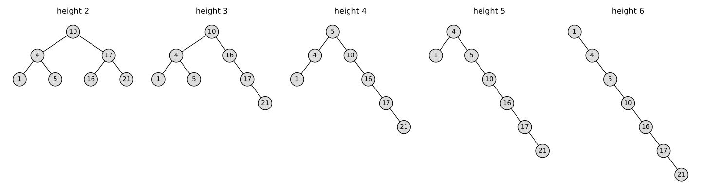
How does the binary-search-tree property differ from the min-heap property (page 153)? Can the min-heap property be used to print the keys of an \(n\)-node tree in sorted order in \(O(n)\) time? Show how, or explain why not.
The binary-search-tree property orders a node against both subtrees in opposite directions, keys in the left subtree \(\le x.key \le\) keys in the right subtree, whereas the min-heap property orders a node in the same direction against both subtrees, \(x.key \le\) every key below it, and says nothing about how the left subtree compares with the right; consequently the min-heap property cannot yield sorted output in \(O(n)\) time.
Indeed, suppose some algorithm \(P\) printed, using only key comparisons, the keys of any \(n\)-node min-heap-ordered tree in sorted order in \(O(n)\) time. Given an arbitrary array of \(n\) keys, BUILD-MIN-HEAP (the min-heap analogue of BUILD-MAX-HEAP, Section 6.3) turns it into such a tree in \(O(n)\) time with comparisons only, and \(P\) then prints it sorted. This is a comparison sort running in
\begin{equation*} O(n) + O(n) = O(n) \end{equation*}
time in the worst case, contradicting the \(\Omega(n \lg n)\) worst-case lower bound for comparison sorts (Theorem 8.1). Hence no such \(P\) exists.
Design an inorder tree walk that does not use recursion. (Hint: a simple approach keeps an auxiliary stack; a trickier but elegant one uses no stack at all, provided pointers can be tested for equality.)
Simulate the recursion with an explicit stack: walk left from the current node pushing every node passed, and when the current pointer becomes NIL, pop a node, print it, and move to its right child.
INORDER-TREE-WALK-ITERATIVE(T)
1  let S be an empty stack
2  x = T.root
3  while x != NIL or S is not empty
4      if x != NIL
5          PUSH(S, x)
6          x = x.left
7      else x = POP(S)
8          print x.key
9          x = x.right
Correctness. Write \(I(z)\) for the inorder key sequence of the subtree rooted at \(z\) (empty if \(z = \text{NIL}\)), and let the stack hold \(y_1, \dots, y_m\) from top to bottom. Loop invariant: at the start of each iteration of the while loop,
\begin{equation*} \text{printed} \cdot I(x) \cdot y_1.key \cdot I(y_1.right) \cdots y_m.key \cdot I(y_m.right) = I(T.root), \end{equation*}
where \(\cdot\) is concatenation.
- Initialization: nothing printed, \(x = T.root\), \(S\) empty.
- Maintenance: (i) if \(x \ne \text{NIL}\), then \(I(x) = I(x.left) \cdot x.key \cdot I(x.right)\), and lines 5-6 replace \(I(x)\) by \(I(x.left)\) while pushing \(x\) on top, which contributes \(x.key \cdot I(x.right)\), so the left side is unchanged; (ii) if \(x = \text{NIL}\), then \(I(x)\) is empty, and lines 7-9 move \(y_1.key\) to the printed sequence and make \(x = y_1.right\), whose \(I(x)\) replaces the term \(I(y_1.right)\).
- Termination: the loop exits when \(x = \text{NIL}\) and \(S\) is empty, so the invariant reads printed \(= I(T.root)\), which is the sorted order by the binary-search-tree property.
That the loop does exit, and how fast, follows from the potential
\begin{equation*} \Phi = 2\,|x| + \sum_{i=1}^{m} \bigl(1 + 2\,|y_i.right|\bigr), \end{equation*}
where \(|z|\) is the number of nodes in the subtree of \(z\). Initially \(\Phi = 2n\). A push iteration changes \(2(1 + |x.left| + |x.right|)\) into \(2|x.left| + 1 + 2|x.right|\), and a pop iteration changes \(1 + 2|y_1.right|\) into \(2|y_1.right|\); either way \(\Phi\) drops by exactly 1. Since \(\Phi = 0\) exactly when \(x = \text{NIL}\) and \(S\) is empty, the loop runs exactly \(2n\) times, each in \(O(1)\) time, so the walk takes \(\Theta(n)\) time.
Write recursive procedures for the preorder and the postorder tree walk, each running in \(\Theta(n)\) time on an \(n\)-node tree.
Move the print statement of INORDER-TREE-WALK before (preorder) or after (postorder) the two recursive calls.
PREORDER-TREE-WALK(x)
1  if x != NIL
2      print x.key
3      PREORDER-TREE-WALK(x.left)
4      PREORDER-TREE-WALK(x.right)

POSTORDER-TREE-WALK(x)
1  if x != NIL
2      POSTORDER-TREE-WALK(x.left)
3      POSTORDER-TREE-WALK(x.right)
4      print x.key
Correctness is immediate by induction on the subtree size: for \(x \ne \text{NIL}\) the procedures print \(x.key\) followed (respectively preceded) by the preorder (postorder) walks of \(x.left\) and \(x.right\), which is the definition of these walks in Section 12.1.
Running time. Each procedure prints every node exactly once, so \(T(n) = \Omega(n)\). On an empty subtree it does a constant amount of work \(c\), and on a node whose left subtree has \(k\) nodes it does \(T(k) + T(n-k-1) + d\) for a constant \(d\) covering the nonrecursive body. This is exactly the recurrence in the proof of Theorem 12.1, whose substitution argument gives \(T(n) \le (c+d)n + c\) verbatim. Hence \(T(n) = \Theta(n)\) for both walks.
Given that, in the comparison model, sorting \(n\) elements requires \(\Omega(n \lg n)\) time in the worst case, argue that every comparison-based algorithm that builds a binary search tree from an arbitrary list of \(n\) elements must take \(\Omega(n \lg n)\) time in the worst case.
A faster construction would give a faster comparison sort. Let \(A\) be a comparison-based algorithm that builds a binary search tree from any list of \(n\) elements in worst-case time \(B(n)\). Sort a list by running \(A\) and then INORDER-TREE-WALK on the root of the resulting tree. The walk outputs the keys in sorted order by the binary-search-tree property, takes \(\Theta(n)\) time by Theorem 12.1, and compares no keys, so the combination is a comparison sort with worst-case running time \(B(n) + O(n)\). By the lower bound for comparison sorting (Theorem 8.1),
\begin{equation*} B(n) + O(n) = \Omega(n \lg n), \qquad\text{so}\qquad B(n) = \Omega(n \lg n). \end{equation*}
12.2 Querying a binary search tree
A binary search tree holds numbers from 1 to 1000, and we search it for 363. Which of the following could not be the sequence of nodes examined by the search?
(a) 2, 252, 401, 398, 330, 344, 397, 363.
(b) 924, 220, 911, 244, 898, 258, 362, 363.
(c) 925, 202, 911, 240, 912, 245, 363.
(d) 2, 399, 387, 219, 266, 382, 381, 278, 363.
(e) 935, 278, 347, 621, 299, 392, 358, 363.
Sequences (c) and (e) are impossible; (a), (b), (d) are possible.
After the search visits key \(v \ne 363\) it moves into the subtree of \(v\) on the side of 363, all of whose keys lie on that side of \(v\) (binary-search-tree property). So every later key must lie strictly inside the open interval \((\ell, u)\), where \(\ell\) is the largest visited key below 363 and \(u\) the smallest visited key above 363. Conversely, if every key respects this, the path itself (each node the child of its predecessor on the side of 363) is a valid binary search tree, so the sequence can occur.
(a) The intervals shrink \((2,\infty) \to (252,\infty) \to (252,401) \to (252,398) \to (330,398) \to (344,398) \to (344,397)\), each new key inside: possible.
(b) \((-\infty,924) \to (220,924) \to (220,911) \to (244,911) \to (244,898) \to (258,898) \to (362,898)\): possible.
(c) After 925, 202, 911 the interval is \((202, 911)\); after 240 it is \((240, 911)\), and \(912 \notin (240,911)\). Concretely, 912 would sit in the left subtree of 911. Impossible.
(d) \((2,\infty) \to (2,399) \to (2,387) \to (219,387) \to (266,387) \to (266,382) \to (266,381) \to (278,381)\): possible.
(e) After 935, 278, 347, 621 the interval is \((347, 621)\), and \(299 \notin (347,621)\): 299 would lie in the right subtree of 347. Impossible.
Give recursive versions of the procedures TREE-MINIMUM and TREE-MAXIMUM.
Recurse into the left (respectively right) child until there is none; as in the book, \(x\) is a non-NIL node.
TREE-MINIMUM(x)
1  if x.left == NIL
2      return x
3  return TREE-MINIMUM(x.left)

TREE-MAXIMUM(x)
1  if x.right == NIL
2      return x
3  return TREE-MAXIMUM(x.right)
Correctness of TREE-MINIMUM is by induction on the height of the subtree rooted at \(x\). If \(x.left = \mathrm{NIL}\), every other key in the subtree lies in \(x\)’s right subtree and so is at least \(x.key\); hence \(x\) is a minimum, as returned in line 2. Otherwise, every key in the right subtree is \(\ge x.key \ge\) every key in the left subtree, so a minimum of the left subtree is a minimum of the whole subtree, and by the inductive hypothesis line 3 returns one. TREE-MAXIMUM is the mirror image (swap left and right and reverse the inequalities).
Each call takes constant time plus one recursive call one level deeper, so a call on the root of a tree of height \(h\) makes at most \(h+1\) calls and runs in \(O(h)\) time, the same as the iterative versions.
Give the procedure TREE-PREDECESSOR.
TREE-PREDECESSOR is TREE-SUCCESSOR with left and right swapped, and with TREE-MAXIMUM in place of TREE-MINIMUM. It returns NIL when \(x\) holds the smallest key.
TREE-PREDECESSOR(x)
1  if x.left != NIL
2      return TREE-MAXIMUM(x.left)
3  y = x.p
4  while y != NIL and x == y.left
5      x = y
6      y = y.p
7  return y
Correctness: let \(T^{\prime}\) be the mirror image of \(T\), with every node’s left and right children swapped and every key \(k\) replaced by \(-k\). Then \(T^{\prime}\) is a binary search tree, and its inorder walk is the reverse of \(T\)’s, so the predecessor of \(x\) in \(T\) is the successor of \(x\) in \(T^{\prime}\). Running TREE-PREDECESSOR\((x)\) on \(T\) performs, step for step, the same pointer moves as TREE-SUCCESSOR\((x)\) on \(T^{\prime}\): TREE-MAXIMUM on \(T\) is TREE-MINIMUM on \(T^{\prime}\), and the test \(x = y.left\) becomes \(x = y.right\). The book proves TREE-SUCCESSOR correct (Theorem 12.2 and Exercise 12.2-6), so TREE-PREDECESSOR is correct too.
Running time: either line 2 follows one path down the tree, or lines 3-6 follow one path up it, so the time is \(O(h)\) on a tree of height \(h\).
Professor Bunyan claims the following about binary search trees. Suppose the search for a key \(k\) ends at a leaf. Let \(A\) be the set of keys to the left of the search path, \(B\) the set of keys on the path, and \(C\) the set of keys to the right of the path. He claims that every choice of \(a \in A\), \(b \in B\), \(c \in C\) satisfies \(a \le b \le c\). Give a smallest possible counterexample.
Four nodes suffice if the claim is read as the two inequalities \(a \le b\) and \(b \le c\) separately: take root 1 with right child 3, where 3 has children 2 (left) and 4 (right), and search for 4. Read literally, the claim is about triples, so \(A\) and \(C\) must both be nonempty, and then six nodes are needed: take root 1 with right child 3, where 3 has children 2 and 5, and 5 has children 4 and 6, and search for 4.
In the four-node tree the path is \(1, 3, 4\), with \(A = \{2\}\) and \(C = \emptyset\), and \(a = 2 > 1 = b\). In the six-node tree the path is \(1, 3, 5, 4\), with \(A = \{2\}\) and \(C = \{6\}\), and the triple \((a,b,c) = (2,1,6)\) fails \(a \le b\).
Minimality. Assume a violation exists. By mirror symmetry we may assume \(a > b\) for some \(a \in A\), \(b \in B\). Since \(a \in A\), \(a\) lies in the left subtree of a path node \(u\) where the path turns right. Every path node at or below \(u\) is \(\ge u > a\), so \(b\) is a proper ancestor of \(u\). Both \(a\) and \(u\) lie in one subtree of \(b\), and \(a > b\), so it is the right subtree and the path turns right at \(b\). Also \(u\) has a left child, so \(u\) is not the leaf where the search ends, and the path continues to \(u\)’s right child \(w\). The nodes \(b, u, a, w\) are distinct, which gives at least 4 nodes; the four-node tree shows 4 is attained.
Under the triple reading, \(C \neq \emptyset\) as well, so some path node \(v\) turns left and has a node \(c\) in its right subtree. Here \(v \ne b, u\), because the path turns right at both of those.
(i) If \(v \ne w\), then \(v\) and \(c\) are two further nodes, since \(c\) hangs off a different path node than \(a\).
(ii) If \(v = w\), the path continues past \(w\) to its left child, and that child and \(c\) are two further nodes.
Either way at least 6 nodes are needed, and the six-node tree attains 6.
Show that if a node of a binary search tree has two children, then its successor has no left child and its predecessor has no right child.
Since \(x.right \ne \mathrm{NIL}\), line 2 of TREE-SUCCESSOR returns \(y = \text{TREE-MINIMUM}(x.right)\). TREE-MINIMUM walks left and stops only at a node whose left child is NIL, so \(y.left = \mathrm{NIL}\). Symmetrically, since \(x.left \ne \mathrm{NIL}\), line 2 of TREE-PREDECESSOR (Exercise 12.2-3) returns \(\text{TREE-MAXIMUM}(x.left)\). TREE-MAXIMUM stops only at a node whose right child is NIL, so the predecessor has no right child.
Let \(T\) be a binary search tree with distinct keys. Suppose node \(x\) of \(T\) has an empty right subtree and has a successor \(y\). Show that \(y\) is the lowest ancestor of \(x\) whose left child is also an ancestor of \(x\). Every node counts as its own ancestor.
In the inorder walk, the node right after \(x\) is the lowest ancestor \(z\) of \(x\) with \(x\) in \(z\)’s left subtree. With distinct keys, the inorder walk lists the keys in strictly increasing order (the binary-search-tree property, Section 12.1), so the node right after \(x\) is its successor \(y\).
Let \(x = z_0, z_1, \dots, z_m\) be the path from \(x\) up to the root, with \(z_i = z_{i-1}.p\). Let \(j\) be the least index with \(z_{j-1} = z_j.left\). Then \(z_j\) is the lowest ancestor of \(x\) whose left child, \(z_{j-1}\), is an ancestor of \(x\). Such a \(j\) exists: otherwise every \(z_{i-1}\) is a right child, so following right pointers from the root leads to \(x\), and \(x.right = \mathrm{NIL}\) makes \(x\) the result of TREE-MAXIMUM on the root. Then \(x\) holds the largest key and has no successor, a contradiction.
For \(1 \le i < j\) we have \(z_{i-1} = z_i.right\), so starting from \(z_{j-1}\) and following right pointers passes through \(z_{j-2}, \dots, z_0 = x\) and stops at \(x\), because \(x.right = \mathrm{NIL}\). So \(x\) is TREE-MAXIMUM\((z_{j-1})\), the last node of the inorder walk of the subtree rooted at \(z_{j-1} = z_j.left\). The inorder walk of the subtree rooted at \(z_j\) is the walk of \(z_j.left\), then \(z_j\), then the walk of \(z_j.right\), so \(z_j\) comes immediately after \(x\) there. This subtree’s walk forms one contiguous stretch of the inorder walk of \(T\), since INORDER-TREE-WALK visits each subtree in a single recursive call. So \(z_j\) comes immediately after \(x\) in the walk of \(T\), and \(z_j = y\).
One way to do an inorder walk of an \(n\)-node binary search tree is to call TREE-MINIMUM to find the smallest element and then call TREE-SUCCESSOR \(n-1\) times. Prove that this method takes \(\Theta(n)\) time.
Every tree edge is traversed at most once downward and at most once upward, so the procedure makes at most \(2(n-1)\) pointer moves and runs in \(\Theta(n)\) time.
Let \(x_1,\dots,x_n\) be the nodes in inorder; the method visits \(x_1 = \) TREE-MINIMUM\((T.root)\) and then \(x_{i+1} = \) TREE-SUCCESSOR\((x_i)\). Each call does \(O(1)\) work plus one unit per edge it walks along (each loop iteration of TREE-MINIMUM moves down one edge, line 3 and each iteration of lines 4–6 of TREE-SUCCESSOR move up one edge). Fix an edge from \(u\) to its child \(c\), and let \(S\) be the subtree rooted at \(c\); its nodes form a contiguous block \(x_a,\dots,x_b\) of the inorder sequence.
(i) Downward moves \(u \to c\). If this happens in the initial TREE-MINIMUM, the descent continues inside \(S\), so \(x_1 \in S\). If it happens in TREE-SUCCESSOR\((x_i)\) (line 2), then \(x_i \notin S\) (either \(x_i = u\) or \(x_i\) is a proper ancestor of \(u\)), while the rest of the descent stays in \(S\), so \(x_{i+1} \in S\). Hence a downward move marks the sequence \(x_1,x_2,\dots\) entering \(S\), either at its start or at an index \(i\) with \(x_i\notin S\), \(x_{i+1}\in S\).
(ii) Upward moves \(c \to u\) happen only in lines 3–6 of TREE-SUCCESSOR\((x_i)\), where \(c\) is an ancestor of \(x_i\) and the returned \(x_{i+1}\) is a proper ancestor of \(c\); so \(x_i \in S\), \(x_{i+1} \notin S\): the sequence leaves \(S\).
Because \(S\) is the contiguous block \(x_a,\dots,x_b\), the sequence enters \(S\) once and leaves it at most once, so the edge is walked at most twice. With \(n-1\) edges,
\begin{equation*} T(n) \le c_1\, n + c_2 \cdot 2(n-1) = O(n), \end{equation*}
and \(T(n) = \Omega(n)\) because the \(n-1\) calls each cost at least a constant. Hence \(T(n) = \Theta(n)\).
Show that, whatever node of a binary search tree of height \(h\) we start from, making \(k\) consecutive calls to TREE-SUCCESSOR costs \(O(k+h)\) time.
The calls touch at most \(k + 2h + 3\) distinct nodes and walk each edge at most twice, so they make \(O(k+h)\) pointer moves and take \(O(k+h)\) time.
Let \(x_0\) be the start node and \(x_{i} = \) TREE-SUCCESSOR\((x_{i-1})\), so \(x_0,\dots,x_k\) are consecutive in inorder. (Only the last call can return NIL, since no call can follow it; by Theorem 12.2 that call costs \(O(h)\), so assume all \(x_i\) exist.) Call \(i\) costs \(O(1)\) plus the number of edges it walks.
Edges are walked at most twice: the argument of Exercise 12.2-7 (a downward move into the subtree \(S\) of a child \(c\) means the sequence \(x_0, x_1,\dots\) enters \(S\), an upward move out of \(S\) means it leaves \(S\), and \(S\) is a contiguous block of the inorder sequence) applies to any run of successor calls.
Touched nodes are few: in call \(i\), the nodes visited are \(x_{i-1}\) together with ancestors of \(x_i\) (line 2: the path from \(x_{i-1}.right\) down to \(x_i\)), or ancestors of \(x_{i-1}\) (lines 3–7). So every touched node \(v\) is an ancestor of some \(x_j\), \(0 \le j \le k\). If \(v\) is an ancestor of neither \(x_0\) nor \(x_k\), the inorder block of \(v\)’s subtree contains \(x_j\) but neither \(x_0\) nor \(x_k\), so it lies strictly between them; hence \(v \in \{x_1,\dots,x_{k-1}\}\). Each of \(x_0\) and \(x_k\) has at most \(h+1\) ancestors, so
\begin{equation*} |V_{\text{touched}}| \le (k+1) + 2(h+1) = k + 2h + 3 . \end{equation*}
Every walked edge joins two touched nodes, and a set of \(m\) tree nodes spans at most \(m-1\) edges, so at most \(k+2h+2\) distinct edges are walked, each at most twice:
\begin{equation*} T \le c_1 k + c_2 \cdot 2(k + 2h + 2) = O(k+h). \end{equation*}
Let \(T\) be a binary search tree with distinct keys, \(x\) a leaf of \(T\), and \(y\) the parent of \(x\). Show that \(y.key\) is either the smallest key of \(T\) exceeding \(x.key\) or the largest key of \(T\) below \(x.key\).
If \(x = y.left\) then \(y\) is the successor of \(x\); if \(x = y.right\) then \(y\) is the predecessor of \(x\).
Suppose \(x = y.left\), so \(x.key < y.key\) by the binary-search-tree property and distinct keys. Assume some node \(z\) has \(x.key < z.key < y.key\); then \(z \ne x, y\). Since \(y\)’s left subtree is \(\{x\}\) and every key in \(y\)’s right subtree is \(\ge y.key\), \(z\) is not in the subtree of \(y\). Let \(w\) be the lowest common ancestor of \(y\) and \(z\); then \(w \ne y\), so \(x\) and \(y\) lie in one child subtree of \(w\), while \(z\) is \(w\) itself or lies in the other one.
(i) \(x, y\) in \(w.left\)’s subtree: \(z.key \ge w.key > y.key\).
(ii) \(x, y\) in \(w.right\)’s subtree: \(z.key \le w.key < x.key\).
Both contradict \(x.key < z.key < y.key\), so \(y.key\) is the smallest key exceeding \(x.key\). The case \(x = y.right\) is symmetric (exchange left/right and reverse all inequalities), giving that \(y.key\) is the largest key below \(x.key\).
12.3 Insertion and deletion
Write a recursive version of the procedure TREE-INSERT.
Recurse down from the root: compare \(z.key\) with the current node \(x\), and hang \(z\) on the side of \(x\) that is NIL, or else recurse into that side.
TREE-INSERT-REC(T, z)
1  if T.root == NIL
2      z.p = NIL
3      T.root = z            // tree T was empty
4  else INSERT-BELOW(T.root, z)

INSERT-BELOW(x, z)           // x is not NIL
1  if z.key < x.key
2      if x.left == NIL
3          x.left = z
4          z.p = x
5      else INSERT-BELOW(x.left, z)
6  elseif x.right == NIL
7      x.right = z
8      z.p = x
9  else INSERT-BELOW(x.right, z)
By induction on the height of the subtree at \(x\), INSERT-BELOW\((x,z)\) attaches \(z\) at the NIL reached from \(x\) by going left when \(z.key < x.key\) and right otherwise: exactly the path of the while loop of TREE-INSERT (lines 3-7), with the attachment of its lines 8-13. Each call does \(O(1)\) work one level deeper, so the time is \(O(h)\).
A binary search tree is built by repeatedly inserting distinct values with TREE-INSERT. Argue that searching the tree for a value examines exactly one more node than inserting that value examined when it first went into the tree.
Both operations follow the same root-to-\(v\) path; insertion stops one node short of it. Let \(z\) be the node holding \(v\), and let \(y_1 = T.root, y_2, \dots, y_k\) be the non-NIL nodes that \(x\) visits in the while loop of TREE-INSERT when \(z\) is inserted; these are the \(k\) nodes examined, and \(z\) becomes a child of \(y_k\), so \(y_1,\dots,y_k\) are exactly the proper ancestors of \(z\).
Later insertions only replace NIL pointers by new leaves (lines 9-13 of TREE-INSERT); they never change an existing parent-child link. Hence for the rest of the tree’s life the root-to-\(z\) path is still \(y_1,\dots,y_k,z\).
TREE-SEARCH\((T.root, v)\) at node \(y_i\) compares \(v\) with \(y_i.key \ne v\) and moves left iff \(v < y_i.key\), which is the same comparison insertion made at \(y_i\) (values are distinct, so the insertion’s tie rule never fired). By induction on \(i\), the search visits \(y_1,\dots,y_k\) and then \(z\), where it stops since \(z.key = v\). It examines
\begin{equation*} k + 1 \end{equation*}
nodes, one more than the \(k\) examined by the insertion.
To sort a set of \(n\) numbers, insert them one at a time into an initially empty binary search tree with TREE-INSERT, and then print them with an inorder tree walk. Find the worst-case and the best-case running times of this sorting method.
Worst case \(\Theta(n^2)\), best case \(\Theta(n \lg n)\). The inorder walk costs \(\Theta(n)\) by Theorem 12.1. By the argument of Exercise 12.3-2, inserting a key examines exactly its proper ancestors in the final tree, so inserting the node \(x_i\) costs \(\Theta(1 + d_i)\), where \(d_i\) is its depth in the final tree, and the total time is
\begin{equation*} \Theta(n + D), \qquad D = \sum_{i=1}^{n} d_i . \end{equation*}
Worst case: the \(i\)-th key inserted has at most \(i-1\) ancestors, so \(D \le \sum_{i=1}^n (i-1) = n(n-1)/2\); inserting the keys in increasing order makes each new key the right child of the previous one, giving a chain with \(D = n(n-1)/2\) exactly. Hence \(\Theta(n^2)\).
Best case: a binary tree has at most \(2^d\) nodes at depth \(d\), hence at most \(2^{d+1}-1\) nodes of depth \(\le d\), so the \(i\)-th shallowest node has depth at least \(\lfloor \lg i \rfloor\). Therefore, for every insertion order,
\begin{equation*} \begin{aligned} D \ge \sum_{i=1}^{n} \lfloor \lg i \rfloor &\ge \sum_{i=\lceil n/2 \rceil}^{n} \Bigl(\lg \frac{n}{2} - 1\Bigr) \ge \frac{n}{2}\,(\lg n - 2) = \Omega(n \lg n). \end{aligned} \end{equation*}
The bound is attained by inserting the median first and then, recursively, the medians of the two halves (level by level): the result has height \(\lfloor \lg n \rfloor\), so \(D \le n \lg n\). Hence the best case is \(\Theta(n \lg n)\).
Is deletion commutative, in the sense that deleting \(x\) and then \(y\) from a binary search tree always yields the same tree as deleting \(y\) and then \(x\)? Prove it or give a counterexample.
No. Take the tree with root \(2\), left child \(1\), right child \(4\), and \(3\) the left child of \(4\), and delete the nodes \(1\) and \(2\) with TREE-DELETE.
(i) Delete \(1\), then \(2\). Node \(1\) is a leaf and simply disappears. Now \(2\) has no left child, so lines 1-2 replace it by its right child: the result is root \(4\) with left child \(3\).
(ii) Delete \(2\), then \(1\). Node \(2\) has two children; its successor is \(y = 3\), with \(y.p = 4 \ne 2\), so lines 7-12 splice \(3\) out, make \(4\) its right child and \(1\) its left child, giving root \(3\) with children \(1\) and \(4\). Deleting the leaf \(1\) leaves root \(3\) with right child \(4\).
The two results (root \(4\) versus root \(3\)) differ, so deletion is not commutative.
Suppose each node \(x\) of a binary search tree stores no parent pointer \(x.p\) but instead a pointer \(x.succ\) to its successor (NIL for the maximum). Give pseudocode for SEARCH, INSERT and DELETE on a tree \(T\) in this representation, each running in \(O(h)\) time, where \(h\) is the height of \(T\). (Hint: a subroutine returning the parent of a node may help.)
SEARCH is TREE-SEARCH unchanged (it never uses \(p\)); INSERT records the last left turn and last right turn on its way down; DELETE first walks from the root to \(z\) to recover its parent \(q\) and the last right turn \(w\), then performs TREE-DELETE with explicit parents and redirects the predecessor’s \(succ\). Keys are assumed distinct, so the walk to \(z\) can be steered by keys.
INSERT(T, z)                   // z.left == z.right == NIL
 1  y = NIL;  x = T.root;  l = NIL;  r = NIL
 2  while x != NIL
 3      y = x
 4      if z.key < x.key
 5          l = x;  x = x.left      // last left turn
 6      else r = x;  x = x.right    // last right turn
 7  if y == NIL            T.root = z
 8  elseif z.key < y.key   y.left = z
 9  else                   y.right = z
10  z.succ = l
11  if r != NIL   r.succ = z
DELETE(T, z)
 1  q = NIL;  w = NIL;  x = T.root
 2  while x != z                    // q = parent of z
 3      q = x
 4      if z.key < x.key   x = x.left
 5      else w = x;  x = x.right    // last right turn
 6  if z.left != NIL   w = TREE-MAXIMUM(z.left)
 7  if w != NIL   w.succ = z.succ   // w = predecessor of z
 8  if z.left == NIL       REPLACE(T, q, z, z.right)
 9  elseif z.right == NIL  REPLACE(T, q, z, z.left)
10  else y = z.succ                 // = TREE-MINIMUM(z.right)
11      if y != z.right
12          r = z.right             // find parent r of y
13          while r.left != y   r = r.left
14          r.left = y.right
15          y.right = z.right
16      REPLACE(T, q, z, y)
17      y.left = z.left

REPLACE(T, q, u, v)                 // q = parent of u
1  if q == NIL            T.root = v
2  elseif u == q.left     q.left = v
3  else                   q.right = v
REPLACE is TRANSPLANT with the parent passed in and the \(v.p\) update dropped. Lines 1-5 of DELETE are the hinted parent subroutine: by the binary-search-tree property the key comparisons steer \(x\) along the root-to-\(z\) path, and \(q\) trails it.
Shape. INSERT builds the same tree as TREE-INSERT (lines 1-9 are its lines 1-13 minus \(z.p\)). DELETE is TREE-DELETE case by case (Figure 12.4): lines 8-9 are cases (a)-(b); in cases (c)-(d) the successor \(y\) is TREE-MINIMUM\((z.right)\) (it has no left child, Exercise 12.2-5), and when \(y \ne z.right\) it lies on the left spine of \(z.right\), so line 13 finds its parent \(r\) and line 14 is TRANSPLANT\((T, y, y.right)\); lines 15-17 are lines 8, 10, 11 of TREE-DELETE.
Successor pointers. Inserting or deleting a single node changes the inorder sequence only by adding or removing that node, so only \(z\) and the predecessor of \(z\) need new \(succ\) values. In INSERT, \(z\) is a leaf, so its predecessor is its lowest ancestor having \(z\) in its right subtree, namely \(r\), and its successor is its lowest ancestor having \(z\) in its left subtree, namely \(l\) (Exercise 12.2-6 and its mirror image); lines 10-11 set \(r.succ = z\) and \(z.succ = l\). In DELETE, the predecessor of \(z\) is TREE-MAXIMUM\((z.left)\) if \(z.left \ne\) NIL, and otherwise the last right turn \(w\) on the root-to-\(z\) path; line 7 sets its \(succ\) to \(z.succ\).
Time. The walks in lines 1-5, line 6 and line 13 of DELETE and the loop of INSERT each move down one level per iteration, and the rest is \(O(1)\), so every operation runs in \(O(h)\).
When the node \(z\) passed to TREE-DELETE has two children, we could take \(y\) to be the predecessor of \(z\) instead of its successor. What further changes to TREE-DELETE would that require? It has been argued that a fair strategy, which gives predecessor and successor equal priority, performs better in practice. How could TREE-DELETE be modified to implement such a fair strategy?
Lines 5-12 must be mirrored, exchanging left and right throughout; lines 1-4 stay. The predecessor of \(z\) is \(y = \) TREE-MAXIMUM\((z.left)\), which has no right child (mirror of Exercise 12.2-5), so it is spliced out by its left child and then adopts \(z\)’s left subtree (if \(y \ne z.left\)) and \(z\)’s right subtree:
 5  else y = TREE-MAXIMUM(z.left)
 6      if y.p != z
 7          TRANSPLANT(T, y, y.left)
 8          y.left = z.left
 9          y.left.p = y
10      TRANSPLANT(T, z, y)
11      y.right = z.right
12      y.right.p = y
Correctness and the \(O(h)\) bound carry over from TREE-DELETE under the left-right mirror image.
For the fair strategy, keep both versions of lines 5-12 and choose between them on each two-child deletion: flip a fair coin (if RANDOM\((0,1) == 0\) use the successor version, else the predecessor version), or keep a global bit that is toggled after every two-child deletion so the two versions alternate. Either choice adds \(O(1)\) time, so TREE-DELETE still runs in \(O(h)\).
12.4 Randomly built binary search trees
Prove equation (12.3): for every integer \(n \ge 0\), \[ \sum_{i=0}^{n-1} \binom{i+3}{3} = \binom{n+3}{4}. \]
Induct on \(n\) using Pascal’s rule \(\binom{m}{4} + \binom{m}{3} = \binom{m+1}{4}\).
For \(n = 0\) the sum is empty and \(\binom{3}{4} = 0\). If the identity holds for \(n\), then
\begin{equation*} \begin{aligned} \sum_{i=0}^{n} \binom{i+3}{3} &= \binom{n+3}{4} + \binom{n+3}{3} \\ &= \binom{n+4}{4} = \binom{(n+1)+3}{4}, \end{aligned} \end{equation*}
which is the identity for \(n+1\). \(\blacksquare\)
Exhibit a binary search tree on \(n\) nodes whose average node depth is \(\Theta(\lg n)\) while its height is \(\omega(\lg n)\). Then give an asymptotic upper bound on the height of any \(n\)-node binary search tree whose average node depth is \(\Theta(\lg n)\).
Take a balanced tree on \(n - k\) nodes with a chain of \(k = \lfloor \sqrt n \rfloor\) nodes hanging off its maximum; in general the height is \(O(\sqrt{n \lg n})\).
Construction. On keys \(1, \dots, n\) with \(m = n - k\), build a complete binary search tree on \(1, \dots, m\) (all depths \(\le \lfloor \lg m \rfloor\)), then insert \(m+1, m+2, \dots, n\) in increasing order: each becomes the right child of the previous one, so key \(m+j\) has depth at most \(\lg n + j\). The height is at least \(k = \lfloor \sqrt n \rfloor = \omega(\lg n)\), and since \(k^2 \le n\),
\begin{equation*} \sum_{x} \operatorname{depth}(x) \le m \lg n + k \lg n + \frac{k(k+1)}{2} \le n \lg n + n , \end{equation*}
so the average depth is at most \(\lg n + 1\). Conversely, in any binary tree fewer than \(2^d\) nodes have depth below \(d\); with \(d = \lfloor \lg n \rfloor - 1\) we have \(2^d \le n/2\), so at least \(n/2\) nodes have depth \(\ge d\) and the average depth is at least \((\lfloor \lg n \rfloor - 1)/2\). Hence the average depth is \(\Theta(\lg n)\).
Upper bound. Suppose the average depth is at most \(c \lg n\) and the height is \(h\). A deepest node and its ancestors occupy depths \(0, 1, \dots, h\), so
\begin{equation*} \begin{aligned} \frac{h(h+1)}{2} &\le \sum_x \operatorname{depth}(x) \le c\, n \lg n \\ \Rightarrow\quad h &\le \sqrt{2c\, n \lg n} = O\bigl(\sqrt{n \lg n}\bigr). \end{aligned} \end{equation*}
(The bound is attained: the construction above with \(k = \lfloor \sqrt{n \lg n} \rfloor\) still has total depth \(\le n\lg n + k \lg n + k(k+1)/2 = O(n \lg n)\).)
Show that choosing a binary search tree on \(n\) keys uniformly at random from all binary search trees on those keys is a different distribution from that of a randomly built binary search tree (insert the keys in an order drawn uniformly from the \(n!\) permutations). Hint: enumerate the cases for \(n = 3\).
For \(n = 3\) the balanced tree has probability \(1/5\) under the uniform choice but \(1/3\) when randomly built.
On keys \(\{1,2,3\}\) there are \(5\) binary search trees, so each has probability \(1/5\) when chosen uniformly. Inserting the six orders gives
| insertion order | resulting tree |
|---|---|
| 1 2 3 | chain \(1 \to 2 \to 3\) (right, right) |
| 1 3 2 | root 1, right child 3, its left child 2 |
| 2 1 3 | root 2, children 1 and 3 |
| 2 3 1 | root 2, children 1 and 3 |
| 3 1 2 | root 3, left child 1, its right child 2 |
| 3 2 1 | chain \(3 \to 2 \to 1\) (left, left) |
so the randomly built tree is the balanced one with probability \(2/6 = 1/3\) and each of the other four with probability \(1/6\). Since \(1/3 \ne 1/5\), the two distributions differ.
Show that \(f(x) = 2^x\) is a convex function.
For \(x, y \in \mathbb{R}\) and \(0 \le \lambda \le 1\), put \(z = \lambda x + (1-\lambda) y\); we must show \(2^z \le \lambda 2^x + (1-\lambda) 2^y\) (the definition on page 1199).
By inequality (3.12), \(e^t \ge 1 + t\), so for every \(u\) \[ 2^u = 2^z e^{(u-z)\ln 2} \ge 2^z \bigl(1 + (u - z)\ln 2\bigr). \] Applying this with \(u = x\) and \(u = y\) and taking the weighted sum,
\begin{equation*} \begin{aligned} \lambda 2^x + (1-\lambda) 2^y &\ge 2^z \bigl(1 + \ln 2\,[\lambda(x - z) + (1-\lambda)(y - z)]\bigr) \\ &= 2^z , \end{aligned} \end{equation*}
because \(\lambda(x-z) + (1-\lambda)(y-z) = z - z = 0\). \(\blacksquare\)
Let RANDOMIZED-QUICKSORT run on a sequence of \(n\) distinct numbers. Prove that, for every constant \(k > 0\), all of the \(n!\) input permutations except an \(O(1/n^k)\) fraction lead to running time \(O(n \lg n)\).
For each constant \(k\) there is a constant \(c\) such that every element takes part in fewer than \(c \lceil \log_{4/3} n \rceil\) partitions except with probability at most \(n^{-k}\), and then the running time is \(O(n \lg n)\). (The wording conflates input and pivot randomness, so we prove the intended statement: on any fixed input, the probability over the pivot choices that the running time exceeds \(O(n\lg n)\) is \(O(1/n^k)\).)
By Lemma 7.1 the running time is \(O(n + X)\), where \(X\) counts the comparisons in line 4 of PARTITION. Each call compares every non-pivot element of its subarray with the pivot exactly once, so \(X = \sum_x D(x)\), where \(D(x)\) is the number of calls in which \(x\) is a non-pivot element.
Fix \(x\), and let \(s_1 = n, s_2, \dots\) be the sizes of the subarrays in the successive calls where \(x\) is a non-pivot element. Then \(s_t \ge 2\) and \(s_{t+1} \le s_t\). Call step \(t\) good if the side of the partition that contains \(x\) has size at most \(3s_t/4\). This holds whenever the pivot’s rank \(r\) satisfies \(\max(r-1, s_t-r) \le 3s_t/4\), that is, \(s_t/4 \le r \le 3s_t/4 + 1\). The number of integers in that range is at least \[ \bigl(\tfrac34 s_t + \tfrac14\bigr) - \bigl(\tfrac14 s_t + \tfrac34\bigr) + 1 \ge \tfrac{s_t}{2}. \] RANDOMIZED-PARTITION picks the pivot uniformly and independently of everything earlier, so given any history that reaches step \(t\), step \(t\) is bad with probability at most \(1/2\). If steps \(1, \dots, m\) all occur and \(g\) of steps \(1, \dots, m-1\) are good, then \(2 \le s_m \le n (3/4)^g\). So at most \(L = \lceil \log_{4/3} n \rceil\) of the first \(m\) steps are good.
It follows that \(D(x) \ge m\) only if some set \(B\) of \(m - L\) steps among the first \(m\) are all bad. Multiplying the conditional probabilities in time order shows that each fixed \(B\) has probability at most \(2^{-(m-L)}\). Take \(m = cL\) with \(c \ge 2\) an integer and use (C.5), \(\binom{m}{L} \le (em/L)^L\):
\begin{equation*} \begin{aligned} \Pr\{D(x) \ge cL\} &\le \binom{cL}{L} 2^{-(c-1)L} \le (ec)^L\, 2^{-(c-1)L} \\ &= 2^{-L\,(c - 1 - \lg(ec))} \le n^{-(c-1-\lg(ec))/\lg(4/3)} , \end{aligned} \end{equation*}
where the last step uses \(L \ge \lg n / \lg(4/3)\) and assumes \(c - 1 - \lg(ec) > 0\). Since \(c - 1 - \lg(ec) \to \infty\), we can fix a constant \(c\) with \(c - 1 - \lg(ec) \ge (k+1)\lg(4/3)\). Then \(\Pr\{D(x) \ge cL\} \le n^{-(k+1)}\), and a union bound over the \(n\) elements gives \[ \Pr\{\exists x : D(x) \ge cL\} \le n \cdot n^{-(k+1)} = n^{-k}. \] Outside this event, \(X < n \cdot cL = O(n \lg n)\), so the running time is \(O(n + X) = O(n \lg n)\). \(\blacksquare\)
Problems for Chapter 12
Binary search trees with equal keys: Equal keys cause trouble for binary search trees.
(a) What is the asymptotic running time of TREE-INSERT when it is used to insert \(n\) items, all with the same key, into an initially empty binary search tree?
To improve TREE-INSERT, test before line 5 whether \(z.key = x.key\), and before line 11 whether \(z.key = y.key\). When equality holds, apply one of the strategies below (stated for line 5, where \(z\) is compared with \(x\); for line 11 replace \(x\) by \(y\)). For each strategy, find the asymptotic time to insert \(n\) items with identical keys into an initially empty tree.
(b) Store a boolean flag \(x.b\) at each node \(x\) and move \(x\) to \(x.left\) or \(x.right\) according to \(x.b\); the flag flips between FALSE and TRUE every time \(x\) is visited during the insertion of a node whose key equals \(x.key\).
(c) Store at \(x\) a list of the nodes whose key equals \(x.key\), and put \(z\) into that list.
(d) Move \(x\) to \(x.left\) or \(x.right\) at random. (Give the worst-case time, and derive the expected time informally.)
Inserting a node at depth \(d\) (root at depth \(0\)) makes \(d\) iterations of the while loop, so it costs \(\Theta(d+1)\); the total cost is \(\Theta(n + \sum_z d(z))\).
(a) \(\Theta(n^2)\). Line 5 sends an equal key to the right (the test \(z.key < x.key\) fails), so the tree is a right-going chain and the \(k\)-th insertion walks the whole chain of \(k-1\) nodes:
\begin{equation*} \sum_{k=1}^{n} (k-1) = \frac{n(n-1)}{2} = \Theta(n^2). \end{equation*}
(b) \(\Theta(n \lg n)\). Say FALSE sends left. The items reaching a node \(x\) after \(x\) itself go alternately left, right, left, …, so if the subtree at \(x\) has \(m\) nodes, its left and right subtrees have \(\lceil (m-1)/2 \rceil\) and \(\lfloor (m-1)/2 \rfloor\) nodes. Induction on \(m\) gives height \(h(m) = \lfloor \lg m \rfloor\), since \(\lceil (m-1)/2\rceil = \lfloor m/2 \rfloor\) and
\begin{equation*} h(m) = 1 + \lfloor \lg \lfloor m/2 \rfloor \rfloor = \lfloor \lg m \rfloor \quad (m \ge 2). \end{equation*}
So every insertion costs \(O(\lg n)\), for \(O(n\lg n)\) in total. In the other direction, any binary tree has at most \(2^d\) nodes at depth \(d\), so at most \(2^{\lfloor \lg n\rfloor - 1}-1 < n/2\) of its nodes have depth below \(\lfloor \lg n \rfloor - 1\), which makes \(\sum_z d(z) = \Omega(n \lg n)\). Hence \(\Theta(n\lg n)\).
(c) \(\Theta(n)\). Every later item matches the root at the first comparison and is added to the head of the root’s list in \(O(1)\) time, so \(n\) insertions cost \(\Theta(n)\).
(d) Worst case \(\Theta(n^2)\): if every coin sends the walk right, we get the chain of part (a). Expected time \(\Theta(n \lg n)\). Since every decision is a fresh fair coin, we can regard item \(k\) as following its own uniformly random infinite bit string \(\beta_k\), read one bit per level. If item \(k\) ends at depth \(D_k > d\), then the node at depth \(d\) on its path is occupied by an earlier item \(j\) whose first \(d\) bits agree with those of \(\beta_k\); each such \(j\) agrees with probability \(2^{-d}\). By a union bound,
\begin{equation*} \Pr\{D_k > d\} \le \min(1, k\,2^{-d}), \end{equation*}
\begin{equation*} \mathrm{E}[D_k] = \sum_{d \ge 0} \Pr\{D_k > d\} \le \lceil \lg k \rceil + 1 + \sum_{d > \lceil \lg k\rceil} k\,2^{-d} \le \lg k + 3 . \end{equation*}
So the expected total is \(O(\sum_k (\lg k + 4)) = O(n \lg n)\). The \(\Omega(n\lg n)\) bound on \(\sum_z d(z)\) from part (b) holds for every tree, so the expected time is \(\Theta(n \lg n)\).
Radix trees: Let \(a = a_0 a_1 \ldots a_p\) and \(b = b_0 b_1 \ldots b_q\) be strings over an ordered set of characters. Call \(a\) lexicographically less than \(b\) if either
(1) some integer \(j\) with \(0 \le j \le \min(p,q)\) has \(a_i = b_i\) for all \(i = 0, 1, \ldots, j-1\) and \(a_j < b_j\), or (2) \(p < q\) and \(a_i = b_i\) for all \(i = 0, 1, \ldots, p\).
For bit strings, for instance, \(10100 < 10110\) by rule 1 (with \(j = 3\)), and \(10100 < 101000\) by rule 2; this is essentially dictionary order.
A radix tree is a binary tree in which a key \(a = a_0 a_1 \ldots a_p\) is found by starting at the root and, at a node of depth \(i\), going left if \(a_i = 0\) and right if \(a_i = 1\). The node reached after reading the whole of \(a\) carries \(a\); nodes whose path spells no stored string are present only to lead to deeper nodes. (Figure 12.5 shows the radix tree for the bit strings \(1011, 10, 011, 100, 0\): the root’s left child is the key \(0\), whose right child is a key-less node whose right child is \(011\); the root’s right child is a key-less node whose left child is \(10\); \(10\) has left child \(100\) and a key-less right child whose right child is \(1011\).) Let \(S\) be a set of distinct bit strings whose lengths add up to \(n\). Show how to sort \(S\) lexicographically in \(\Theta(n)\) time using a radix tree. For the strings of Figure 12.5 the output should be \(0, 011, 10, 100, 1011\).
Insert every string of \(S\) into an initially empty radix tree, marking the node where each string ends, and then walk the tree in preorder, printing the string of each marked node as we reach it.
RADIX-SORT(S)
 1  T.root = NEW-NODE()                // mark = FALSE, no children
 2  for each string s in S
 3      x = T.root
 4      for i = 0 to s.length - 1
 5          if s[i] == 0
 6              if x.left == NIL then x.left = NEW-NODE()
 7              x = x.left
 8          else
 9              if x.right == NIL then x.right = NEW-NODE()
10              x = x.right
11      x.mark = TRUE
12  PREORDER(T.root, empty string)

PREORDER(x, prefix)
 1  if x == NIL  return
 2  if x.mark  print prefix
 3  PREORDER(x.left, prefix + 0)
 4  PREORDER(x.right, prefix + 1)
Correctness. Each node \(x\) corresponds to the bit string \(\pi(x)\) spelled by its root path, and the marked nodes are exactly the strings of \(S\). Let \(a \ne b\) be marked strings with \(a < b\), and let \(x\) be the deepest common ancestor of their nodes; then \(\pi(x)\) is their longest common prefix. Under rule 2, \(a = \pi(x)\) is the node \(x\) itself, and preorder prints \(x\) before anything in its subtrees. Under rule 1, \(a_j = 0\) and \(b_j = 1\) where \(j = |\pi(x)|\), so \(a\) lies in the left subtree of \(x\) and \(b\) in the right one, and preorder finishes the left subtree before starting the right. In both cases \(a\) is printed before \(b\).
Running time. Inserting a string of length \(\ell\) takes \(O(\ell + 1)\) time and creates at most \(\ell\) nodes, so building the tree costs \(O(n + |S|)\) and the tree has at most \(n + 1\) nodes. Since the strings are distinct, at most one of them is empty, so \(|S| \le n + 1\). Pass the prefix as a single shared buffer that gets one bit pushed before each recursive call and popped after it. The walk then does \(O(1)\) work per node plus \(|a|\) to print each \(a\), so it costs \(O(n + 1) + \sum_{a \in S} |a| = O(n)\). Reading the input already takes \(\Omega(n)\), so the total is \(\Theta(n)\).
Average node depth in a randomly built binary search tree: we show that a node of a randomly built binary search tree on \(n\) nodes has average depth \(O(\lg n)\). This is weaker than Theorem 12.4, but the method exposes a close parallel between building a binary search tree and running RANDOMIZED-QUICKSORT (Section 7.3). The total path length \(P(T)\) of a binary tree \(T\) is the sum, over all nodes \(x\) of \(T\), of the depth \(d(x,T)\) of \(x\) in \(T\).
(a) Argue that the average depth of a node of \(T\) equals
\begin{equation*} \frac{1}{n}\sum_{x\in T} d(x,T) = \frac{1}{n}P(T), \end{equation*}
so that it suffices to show that the expected value of \(P(T)\) is \(O(n\lg n)\).
(b) Writing \(T_L\) and \(T_R\) for the left and right subtrees of \(T\), argue that if \(T\) has \(n\) nodes then \(P(T) = P(T_L) + P(T_R) + n - 1\).
(c) Let \(P(n)\) be the average total path length of a randomly built binary search tree on \(n\) nodes. Show that
\begin{equation*} P(n) = \frac{1}{n}\sum_{i=0}^{n-1}\bigl(P(i) + P(n-i-1) + n - 1\bigr). \end{equation*}
(d) Show that \(P(n)\) can be rewritten as
\begin{equation*} P(n) = \frac{2}{n}\sum_{k=1}^{n-1}P(k) + \Theta(n). \end{equation*}
(e) Using the alternative analysis of randomized quicksort from Problem 7-3, conclude that \(P(n) = O(n\lg n)\).
Each recursive call of quicksort partitions its elements around a random pivot, just as each node of a binary search tree partitions the elements that land in its subtree.
(f) Describe an implementation of quicksort whose comparisons, when sorting a set of elements, are exactly the comparisons made when inserting those elements into a binary search tree (possibly in a different order, but the same set of comparisons).
(a) The average of the \(n\) depths is their sum divided by \(n\), and that sum is \(P(T)\) by definition:
\begin{equation*} \frac{1}{n}\sum_{x\in T} d(x,T) = \frac{1}{n}P(T). \end{equation*}
Taking expectations over the random tree, the expected average depth is \(\mathrm{E}[P(T)]/n\), which is \(O(\lg n)\) exactly when \(\mathrm{E}[P(T)] = O(n\lg n)\).
(b) The root has depth \(0\), and every other node lies in \(T_L\) or \(T_R\) at depth one more than its depth in that subtree; since \(|T_L| + |T_R| = n-1\),
\begin{equation*} \begin{aligned} P(T) &= \sum_{x\in T_L}\bigl(d(x,T_L)+1\bigr) + \sum_{x\in T_R}\bigl(d(x,T_R)+1\bigr)\\ &= P(T_L) + P(T_R) + |T_L| + |T_R| = P(T_L) + P(T_R) + n - 1 . \end{aligned} \end{equation*}
(c) A randomly built tree inserts \(n\) distinct keys in a uniformly random order (Section 12.4). The root is the first key inserted, so its rank is uniform on \(\{1,\dots,n\}\); when it has rank \(i+1\), \(T_L\) holds the \(i\) smaller keys and \(T_R\) the \(n-i-1\) larger ones. Every later key smaller than the root goes left at the root, so \(T_L\) is exactly the tree obtained by inserting the \(i\) smaller keys in their relative order of arrival, and likewise for \(T_R\). Conditioned on the identity of the first key, the relative orders of the smaller and of the larger keys are uniformly random permutations, so \(T_L\) and \(T_R\) are randomly built trees on \(i\) and \(n-i-1\) nodes. Hence, by (b) and the law of total expectation,
\begin{equation*} \begin{aligned} P(n) &= \sum_{i=0}^{n-1}\frac{1}{n}\,\mathrm{E}\bigl[P(T_L)+P(T_R)+n-1 \bigm| |T_L| = i\bigr]\\ &= \frac{1}{n}\sum_{i=0}^{n-1}\bigl(P(i) + P(n-i-1) + n - 1\bigr). \end{aligned} \end{equation*}
(d) As \(i\) runs over \(0,\dots,n-1\) so does \(n-i-1\), so the two sums of \(P\) coincide; with \(P(0) = 0\),
\begin{equation*} P(n) = \frac{2}{n}\sum_{k=0}^{n-1}P(k) + (n-1) = \frac{2}{n}\sum_{k=1}^{n-1}P(k) + \Theta(n). \end{equation*}
(e) Since \(P(1) = 0\), (d) reads \(P(n) = \frac{2}{n}\sum_{k=2}^{n-1}P(k) + (n-1)\), which is recurrence (7.6) of Problem 7-3(c) with \(\mathrm{E}[T(q)]\) replaced by \(P(q)\) and the \(\Theta(n)\) term equal to \(n-1\); so the substitution of Problem 7-3(e) applies. We show \(P(n) \le 4n\lg n\) for all \(n \ge 2\) by induction. Base: \(P(2) = \frac{2}{2}P(1) + 1 = 1 \le 8\). Step (\(n \ge 3\)): assuming \(P(k) \le 4k\lg k\) for \(2 \le k \le n-1\), inequality (7.7) of Problem 7-3(d) gives
\begin{equation*} \begin{aligned} P(n) &\le \frac{8}{n}\sum_{k=2}^{n-1}k\lg k + n - 1 \le \frac{8}{n}\Bigl(\frac{1}{2}n^2\lg n - \frac{1}{8}n^2\Bigr) + n - 1\\ &= 4n\lg n - n + n - 1 < 4n\lg n . \end{aligned} \end{equation*}
Hence \(P(n) = O(n\lg n)\), and by (a) the average node depth of a randomly built binary search tree is \(O(\lg n)\).
(f) Use as pivot the first element of the current input sequence (in insertion order), and partition stably, so each side keeps the elements in their original relative order:
BST-QUICKSORT(S)               // S = <s_1, ..., s_m>, distinct keys
1  if S.length <= 1
2      return S
3  x = S[1]                    // pivot = first element
4  L = empty sequence
5  R = empty sequence
6  for i = 2 to S.length
7      if S[i] < x             // the comparison TREE-INSERT makes at x
8          append S[i] to L    // L, R keep their relative order
9      else append S[i] to R
10 return BST-QUICKSORT(L), then x, then BST-QUICKSORT(R)
Running it on a sequence makes exactly the comparisons that TREE-INSERT makes when the keys are inserted in that order. For a randomized version, first permute the input uniformly at random (RANDOMIZE-IN-PLACE, Section 5.3); every pivot is then a uniformly random element of its subarray, as in RANDOMIZED-QUICKSORT, and the BST matched is a randomly built one.
Inducting on \(m = |S|\): TREE-INSERT compares a key with exactly its proper ancestors, so building \(\mathrm{BST}(S)\) (insert \(S\) in order) compares exactly the (ancestor, descendant) pairs, each once. By (c), \(\mathrm{BST}(S)\) has root \(s_1\) and subtrees \(\mathrm{BST}(L)\), \(\mathrm{BST}( R)\) for the very subsequences \(L\), \(R\) built in lines 4-9. BST-QUICKSORT compares \(s_1\) once with each other key (the descendants of the root) and, by induction, the recursive calls compare exactly the (ancestor, descendant) pairs of \(\mathrm{BST}(L)\) and \(\mathrm{BST}( R)\); together these are all such pairs of \(\mathrm{BST}(S)\), and the output is sorted since \(L < s_1 < R\).
Number of different binary trees: write \(b_n\) for the number of distinct binary trees on \(n\) nodes. The goal is an exact formula for \(b_n\) and an asymptotic estimate.
(a) Prove that \(b_0 = 1\) and that for every \(n \ge 1\) \[ b_n = \sum_{k=0}^{n-1} b_k\, b_{n-1-k}. \]
(b) With generating functions as defined in Problem 4-4, set \(B(x) = \sum_{n=0}^{\infty} b_n x^n\). Prove that \(B(x) = x B(x)^2 + 1\), and deduce that one closed form is \[ B(x) = \frac{1}{2x}\left(1 - \sqrt{1-4x}\right). \]
The Taylor expansion of \(f\) about \(x = a\) is \(f(x) = \sum_{k=0}^{\infty} \frac{f^{(k)}(a)}{k!}(x-a)^k\), where \(f^{(k)}(a)\) is the \(k\)th derivative of \(f\) at \(a\).
(c) Using the Taylor expansion of \(\sqrt{1-4x}\) about \(x = 0\), prove that \[ b_n = \frac{1}{n+1}\binom{2n}{n}, \] the \(n\)th Catalan number. (Alternatively one may use the binomial expansion (C.4) extended to non-integral exponents \(n\), where for real \(n\) and integer \(k\) the symbol \(\binom{n}{k}\) means \(n(n-1)\cdots(n-k+1)/k!\) when \(k \ge 0\) and \(0\) otherwise.)
(d) Prove that \[ b_n = \frac{4^n}{\sqrt{\pi}\, n^{3/2}}\bigl(1 + O(1/n)\bigr). \]
(a) A binary tree is either empty or a root together with an ordered pair (left subtree, right subtree) of binary trees (Appendix B.5.3). There is exactly one empty tree, so \(b_0 = 1\). For \(n \ge 1\), a tree on \(n\) nodes is determined uniquely by its left subtree, with some \(k \in \{0,\dots,n-1\}\) nodes, and its right subtree, with the remaining \(n-1-k\) nodes, and every such pair occurs. Summing the \(b_k b_{n-1-k}\) choices over \(k\) gives the recurrence.
(b) Compare coefficients. The constant term of \(xB(x)^2\) is \(0\), and for \(n \ge 1\), by (a), \[ [x^n]\, xB(x)^2 = [x^{n-1}]\, B(x)^2 = \sum_{k=0}^{n-1} b_k b_{n-1-k} = b_n , \] so \(xB(x)^2 + 1 = B(x)\). As a quadratic in \(B\), \(xB^2 - B + 1 = 0\), so \[ B(x) = \frac{1 \pm \sqrt{1-4x}}{2x}. \] The plus sign blows up as \(x \to 0\), while \(B(0) = b_0 = 1\), so we take the minus sign. (As formal power series: \(B = 1 + xB^2\) fixes every coefficient recursively, and \((1-\sqrt{1-4x})/(2x)\), a power series by (c), satisfies it, so the two are equal.)
(c) By the generalized binomial theorem, \(\sqrt{1-4x} = \sum_{k \ge 0} \binom{1/2}{k}(-4x)^k\); this is also the Taylor series at \(0\), since the \(k\)th derivative of \((1-4x)^{1/2}\) at \(0\) is \(k!\binom{1/2}{k}(-4)^k\). For \(k \ge 1\), use \(1\cdot 3 \cdots (2k-3) = (2k-2)!/(2^{k-1}(k-1)!)\):
\begin{equation*} \begin{aligned} \binom{1/2}{k}(-4)^k &= \frac{\tfrac12\left(-\tfrac12\right)\left(-\tfrac32\right)\cdots\left(\tfrac{3-2k}{2}\right)}{k!}\,(-1)^k 4^k \\ &= \frac{(-1)^{k-1}\, 1\cdot 3\cdots(2k-3)}{2^k\, k!}\,(-1)^k 2^{2k} = -\frac{2^k\,(2k-2)!}{k!\; 2^{k-1}(k-1)!} \\ &= -\frac{2}{k}\binom{2k-2}{k-1}. \end{aligned} \end{equation*}
Hence \(1 - \sqrt{1-4x} = \sum_{k \ge 1} \frac{2}{k}\binom{2k-2}{k-1} x^k\). Dividing by \(2x\) and putting \(n = k-1\), \[ B(x) = \sum_{k\ge 1} \frac{1}{k}\binom{2k-2}{k-1}x^{k-1} = \sum_{n \ge 0} \frac{1}{n+1}\binom{2n}{n} x^n , \] and comparing coefficients gives \(b_n = \frac{1}{n+1}\binom{2n}{n}\).
(d) By Stirling’s approximation (3.18), \(m! = \sqrt{2\pi m}\,(m/e)^m(1+\Theta(1/m))\). Since \(1/(1+O(1/n)) = 1 + O(1/n)\) and \(\Theta(1/(2n)) = \Theta(1/n)\),
\begin{equation*} \begin{aligned} \binom{2n}{n} = \frac{(2n)!}{(n!)^2} &= \frac{\sqrt{4\pi n}\,(2n/e)^{2n}\,(1+O(1/n))}{2\pi n\,(n/e)^{2n}\,(1+O(1/n))^2} \\ &= \frac{4^n}{\sqrt{\pi n}}\bigl(1+O(1/n)\bigr). \end{aligned} \end{equation*}
Also \(\frac{1}{n+1} = \frac{1}{n}\left(1 - \frac{1}{n+1}\right) = \frac{1}{n}(1+O(1/n))\). Multiplying, \[ b_n = \frac{1}{n+1}\binom{2n}{n} = \frac{4^n}{\sqrt{\pi}\,n^{3/2}}\bigl(1+O(1/n)\bigr). \]
Chapter 13: Red-Black Trees
13.1 Properties of red-black trees
Using the drawing conventions of Figure 13.1(a) (every node annotated with its black-height), draw the complete binary search tree of height 3 whose keys are \(\{1, 2, \ldots, 15\}\). Include the NIL leaves, and give three different colorings of its nodes that make it a red-black tree of black-height 2, 3 and 4 respectively.
The tree has root 8, then 4, 12 at depth 1, then 2, 6, 10, 14 at depth 2, then the odd keys \(1, 3, \ldots, 15\) at depth 3, with 16 NIL leaves below; color by depth:
| black-height | depth 0 | depth 1 | depth 2 | depth 3 |
|---|---|---|---|---|
| 2 | black | red | black | red |
| 3 | black | black | black | red |
| 4 | black | black | black | black |
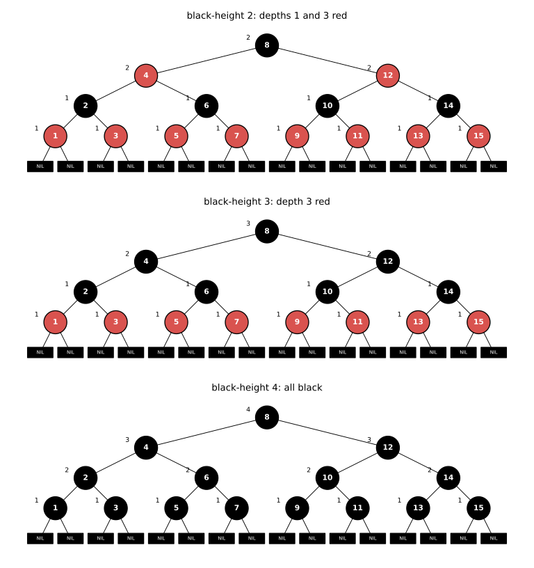
In each coloring the root and the NIL leaves are black (properties 1, 2, 3), no two consecutive depths are both red, so every red node has black children (property 4), and since the coloring depends only on depth and all leaves sit at depth 4, every root-to-leaf path meets the same colors (property 5). Counting the black nodes below the root on such a path, including the NIL, gives \(2\) (depth 2 and the NIL), \(3\) (depths 1, 2 and the NIL) and \(4\) (depths 1, 2, 3 and the NIL), as annotated in the figure.
Take the red-black tree of Figure 13.1: root 26 (black) with children 17 (red) and 41 (black); 17 has children 14 and 21 (black); 14 has children 10 (red) and 16 (black); 10 has children 7 and 12 (black); 7 has left child 3 (red); 16 has left child 15 (red); 21 has children 19 and 23 (black); 19 has right child 20 (red); 41 has children 30 (red) and 47 (black); 30 has children 28 and 38 (black); 38 has children 35 and 39 (red). Draw the tree obtained by calling TREE-INSERT on it with key 36. Is the result a red-black tree if the new node is colored red? If it is colored black?
TREE-INSERT follows the search path \(26 \to 41 \to 30 \to 38 \to 35\) (\(36 > 26\), \(36 < 41\), \(36 > 30\), \(36 < 38\), \(36 > 35\)) and makes 36 the right child of the red node 35 (dashed below); in neither coloring is the result a red-black tree.
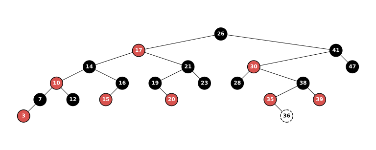
(i) 36 red: its parent 35 is red, so a red node has a red child, violating property 4.
(ii) 36 black: from the red node 35, the path to its left NIL leaf contains one black node (the NIL), while the path through 36 to one of its NIL leaves contains two (36 and the NIL), violating property 5.
Call a binary search tree a relaxed red-black tree if it satisfies red-black properties 1, 3, 4 and 5 (so the root may be red or black). Let \(T\) be a relaxed red-black tree whose root is red. If the root of \(T\) is recolored black and nothing else is changed, is the result a red-black tree?
Yes. Property 2 now holds, and properties 1 and 3 are untouched. Property 4 constrains only red nodes, and the recoloring creates no red node (it removes one), so it still holds. For property 5, a simple path from a node \(x\) to a descendant leaf passes through the root only if \(x\) is the root, and the black-height of \(x\) does not count \(x\) itself; hence every such count is unchanged and property 5 still holds.
In a red-black tree, merge every red node into its (black) parent, so that the children of the red node become children of that black parent (keys are ignored). After all red children of a black node have been absorbed, what degrees can that black node have? What can be said about the depths of the leaves of the tree that results?
An internal black node ends up with 2, 3 or 4 children, and all leaves of the resulting tree have the same depth, namely the black-height of the original root.
A red node has a black parent and, by property 4, two black children, so after absorption only black nodes remain and each child of an internal black node \(x\) contributes:
(i) a black child: 1 child of \(x\);
(ii) a red child: its 2 black children.
With two children each contributing 1 or 2, the degree of \(x\) lies in \(\{2, 3, 4\}\), and all three values occur (both children black; one red; both red). The NIL leaves stay leaves, of degree 0.
An edge of the new tree joins a black node to the next black node on the original downward path, so the depth of a leaf in the new tree equals the number of black nodes strictly below the (black) root on the original root-to-leaf path. By property 5 this equals \(\text{bh}(\text{root})\) for every leaf.
Prove that, for any node \(x\) of a red-black tree, the longest simple path from \(x\) down to a descendant leaf is at most twice as long as the shortest simple path from \(x\) down to a descendant leaf.
Both lengths are squeezed between \(b = \text{bh}(x)\) and \(2b\). Let \(x = v_0, v_1, \ldots, v_L\) be any simple path from \(x\) to a descendant leaf \(v_L\); its length is \(L\). By property 5 exactly \(b\) of \(v_1, \ldots, v_L\) are black, so \(L \ge b\). By property 3 the leaf \(v_L\) is black, and by property 4 every red \(v_i\) with \(1 \le i < L\) has a black successor \(v_{i+1}\); the map \(v_i \mapsto v_{i+1}\) is injective from red nodes to black nodes among \(v_1, \ldots, v_L\), so at most \(b\) of them are red and \(L \le 2b\). Hence
\begin{equation*} \text{longest} \le 2b \le 2 \cdot \text{shortest}. \end{equation*}
For a red-black tree of black-height \(k\), what is the largest possible number of internal nodes? What is the smallest possible number?
The largest number is \(2^{2k} - 1\) and the smallest is \(2^k - 1\).
Lower bound: the proof of Lemma 13.1 shows that the subtree rooted at any node \(x\) has at least \(2^{\text{bh}(x)} - 1\) internal nodes; apply it to the root. It is attained by the complete binary tree of height \(k-1\) with every node black: its black-height is \((k-1) + 1 = k\) (the \(k-1\) internal nodes below the root plus the NIL), and it has \(2^k - 1\) nodes.
Upper bound: by the argument of Exercise 13.1-5 applied to the root, every root-to-leaf path has length at most \(2k\), so every path contains at most \(2k\) internal nodes and the internal nodes form a binary tree of height at most \(2k - 1\), which has at most \(2^{2k} - 1\) nodes. It is attained by the complete binary tree of height \(2k - 1\) whose even depths \(0, 2, \ldots, 2k-2\) are black and odd depths \(1, 3, \ldots, 2k-1\) are red: the root is black, each red node’s children are black (the next depth or the NIL leaves), and each root-to-leaf path has \(k - 1\) black internal nodes below the root plus the NIL, so the black-height is \(k\).
Give a red-black tree on \(n\) keys for which the ratio of red internal nodes to black internal nodes is as large as possible, and state that ratio. Which tree makes the ratio as small as possible, and what is the ratio then?
The largest ratio is \(2\), attained by the perfect tree of height \(2h-1\) (so \(n=4^h-1\)) whose even levels are black and odd levels red; the smallest ratio is \(0\), attained by a perfect all-black tree (\(n=2^k-1\)).
Let \(r\) and \(b\) count the red and black internal nodes. The root is black (property 2), so every red node has a parent, and that parent is black (property 4). Mapping each red node to its parent sends at most two red nodes to each black node, hence
\begin{equation*} r \le 2b, \qquad \frac{r}{b} \le 2 . \end{equation*}
Equality holds iff every black internal node has two red (internal) children. Then colours strictly alternate black, red, black, red, … down every path, and every \(T.nil\) hangs below a red node. By property 5 all paths from the root to a leaf contain the same number \(h\) of black internal nodes, so every leaf sits at depth \(2h\): the tree is perfect of height \(2h-1\), black on levels \(0,2,\dots,2h-2\) and red on levels \(1,3,\dots,2h-1\). Conversely this tree satisfies properties 1-5 (Check!), and
\begin{equation*} b=\sum_{j=0}^{h-1}4^{j}=\frac{4^h-1}{3}, \qquad r=\sum_{j=0}^{h-1}2\cdot 4^{j}=\frac{2(4^h-1)}{3}, \qquad n=4^h-1 . \end{equation*}
The smallest example is a black root with two red children (\(n=3\)).
For the minimum, \(r\ge 0\) trivially, and \(r=0\) means every node is black; property 5 then puts every leaf at the same depth, so the tree is the perfect binary tree of height \(k-1\) with \(n=2^k-1\) keys, all coloured black, which is a valid red-black tree with ratio \(0/(2^k-1)=0\).
For all other \(n\) the two extremes lie strictly inside \((0,2)\): ratio \(2\) forces \(n=4^h-1\) and ratio \(0\) forces \(n=2^k-1\), as just shown.
13.2 Rotations
Give pseudocode for the procedure RIGHT-ROTATE\((T,y)\), the mirror image of LEFT-ROTATE in Section 13.2.
Swap left and right everywhere in LEFT-ROTATE, and swap the roles of \(x\) and \(y\). As in the book, we assume \(y.left \ne T.nil\) and that the root’s parent is \(T.nil\).
RIGHT-ROTATE(T, y)
 1  x = y.left               // set x
 2  y.left = x.right         // turn x's right subtree into y's left subtree
 3  if x.right != T.nil
 4      x.right.p = y
 5  x.p = y.p                // link y's parent to x
 6  if y.p == T.nil
 7      T.root = x
 8  elseif y == y.p.right
 9      y.p.right = x
10  else y.p.left = x
11  x.right = y              // put y on x's right
12  y.p = x
This turns the left configuration of Figure 13.2 into the right one: \(\beta\) moves from \(x\)’s right to \(y\)’s left (lines 2-4), \(x\) takes \(y\)’s place under \(y\)’s old parent (lines 5-10), and \(y\) becomes \(x\)’s right child (lines 11-12).
Show that every binary search tree with \(n\) nodes admits exactly \(n-1\) possible rotations.
Possible rotations are in one-to-one correspondence with the \(n-1\) edges of the tree. LEFT-ROTATE\((T,x)\) can be applied exactly when \(x.right \ne T.nil\), and RIGHT-ROTATE\((T,y)\) exactly when \(y.left \ne T.nil\). So each edge from a parent \(u\) to a child \(v\) allows exactly one rotation: LEFT-ROTATE\((T,u)\) if \(v = u.right\), RIGHT-ROTATE\((T,u)\) if \(v = u.left\). Conversely, every applicable rotation comes from exactly one such edge. Every node other than the root has exactly one parent edge, so
\begin{equation*} \#\{\text{rotations}\} = \#\{\text{non-nil left children}\} + \#\{\text{non-nil right children}\} = n-1 . \end{equation*}
In the right-hand tree of Figure 13.2, node \(x\) has left subtree \(\alpha\) and right child \(y\), and \(y\) has left subtree \(\beta\) and right subtree \(\gamma\). Let \(a\), \(b\), \(c\) be any nodes of \(\alpha\), \(\beta\), \(\gamma\) respectively. When LEFT-ROTATE is applied to \(x\), how do the depths of \(a\), \(b\) and \(c\) change?
The depth of \(a\) increases by \(1\), the depth of \(b\) is unchanged, and the depth of \(c\) decreases by \(1\). Let \(x\) have depth \(d\). Nothing above the rotated subtree changes, and the inside of each of \(\alpha,\beta,\gamma\) is unchanged, so only the depths of the subtree roots matter:
\begin{equation*} \begin{aligned} &\text{before: } x:d,\quad y:d+1,\quad \alpha:d+1,\quad \beta:d+2,\quad \gamma:d+2,\\ &\text{after: } y:d,\quad x:d+1,\quad \alpha:d+2,\quad \beta:d+2,\quad \gamma:d+1 . \end{aligned} \end{equation*}
Prove that any binary search tree with \(n\) nodes can be turned into any other \(n\)-node binary search tree on the same keys using \(O(n)\) rotations. (Hint: first show that at most \(n-1\) right rotations are enough to turn a tree into a right-going chain.)
At most \(2n-2\) rotations are enough: at most \(n-1\) right rotations take \(T_1\) to the right-going chain, and at most \(n-1\) left rotations take the chain to \(T_2\).
Call the path from the root that follows only right pointers the right spine. A tree is a right-going chain exactly when all \(n\) nodes are on the spine. Rotations preserve the in-order key sequence (Figure 13.2), so the chain we reach is the unique right-going chain on the sorted keys, and it is the same for \(T_1\) and \(T_2\).
Suppose some spine node \(y\) has a left child \(x\), and apply RIGHT-ROTATE\((T,y)\). Then \(x\) takes \(y\)’s place on the spine and \(y\) becomes \(x.right\), keeping its right subtree. The spine nodes above \(y\) and below \(y\) stay on the spine, so the spine gains exactly the one node \(x\). The spine starts with at least \(1\) node and can hold at most \(n\), so after at most \(n-1\) such rotations no spine node has a left child, which means the tree is the chain.
Do the same to \(T_2\), obtaining right rotations \(\rho_1,\dots,\rho_k\) with \(k\le n-1\) that take \(T_2\) to the chain. A right rotation at \(y\) is undone by a left rotation at its new subtree root \(x\) (Figure 13.2). Applying these inverses in the order \(\rho_k^{-1},\dots,\rho_1^{-1}\) takes the chain back to \(T_2\). Altogether
\begin{equation*} T_1 \xrightarrow{\ \le n-1\ \text{right}\ } \text{chain} \xrightarrow{\ \le n-1\ \text{left}\ } T_2, \qquad\text{at most } 2n-2 = O(n) \text{ rotations.} \end{equation*}
A binary search tree \(T_1\) can be right-converted to a binary search tree \(T_2\) if some sequence of RIGHT-ROTATE calls turns \(T_1\) into \(T_2\). Give two trees \(T_1\), \(T_2\) such that \(T_1\) cannot be right-converted to \(T_2\). Then prove that if \(T_1\) can be right-converted to \(T_2\), it can be done with \(O(n^2)\) calls to RIGHT-ROTATE.
Example: let \(T_1\) have root \(1\) with right child \(2\), and let \(T_2\) have root \(2\) with left child \(1\). Every right rotation needs a node with a non-nil left child, and \(T_1\) has none. So no right rotation can be applied to \(T_1\), and since \(T_1\ne T_2\), \(T_1\) cannot be right-converted to \(T_2\).
For the bound, we show that every sequence of right rotations on an \(n\)-node tree has length at most \(\binom n2\), which covers in particular any sequence turning \(T_1\) into \(T_2\). Let
\begin{equation*} \Phi(T) = \#\{(u,v) : v \text{ is in the left subtree of } u\} = \sum_{u} |\text{left subtree of } u| . \end{equation*}
Then \(0\le\Phi(T)\le\binom n2\), because each unordered pair of nodes is counted at most once.
Apply RIGHT-ROTATE\((T,y)\) to the configuration of Figure 13.2, where \(x=y.left\) has subtrees \(\alpha,\beta\) and \(y\) has right subtree \(\gamma\). (i) If \(w\) is a proper ancestor of \(y\), the rotated subtree has the same node set and sits on the same side of \(w\), so pairs \((w,\cdot)\) are unchanged. (ii) Pairs with both nodes inside \(\alpha\), \(\beta\) or \(\gamma\) are unchanged. (iii) Pairs headed by \(x\): \(\alpha\) is still \(x\)’s left subtree, so no change. (iv) Pairs headed by \(y\): \(y\)’s left subtree shrinks from \(\{x\}\cup\alpha\cup\beta\) to \(\beta\). Hence
\begin{equation*} \Phi(T^{\prime}) = \Phi(T) - (1+|\alpha|) \le \Phi(T) - 1 . \end{equation*}
\(\Phi\) is a nonnegative integer that every right rotation lowers by at least \(1\), so any right-converting sequence from \(T_1\) has at most \(\Phi(T_1)\le n(n-1)/2 = O(n^2)\) calls to RIGHT-ROTATE.
13.3 Insertion
Line 16 of RB-INSERT colors the newly inserted node \(z\) red. Had we colored \(z\) black instead, property 4 (a red node has only black children) could not be violated. Why is \(z\) nevertheless colored red rather than black?
Because a black \(z\) would break property 5 instead, and that violation is global rather than local. Before the insertion the tree is a valid red-black tree; \(z\) replaces a black sentinel leaf at the bottom of some path, so every simple path from an ancestor of \(z\) down through \(z\) to a leaf would gain one black node,
\begin{equation*} \text{bh along paths through } z = \text{bh elsewhere} + 1 , \end{equation*}
for every ancestor of \(z\) at once (unless \(z\) is the root). Repairing that requires rebalancing black counts all the way up the tree, with no simple local rule.
Coloring \(z\) red keeps property 5 intact (a red node contributes nothing to black-heights, and its two children are the black sentinel, exactly as the leaf it replaced), and the only possible violations are property 2 (\(z\) is the root) or property 4 (\(z.p\) is red). Both are confined to \(z\) and its parent, and RB-INSERT-FIXUP removes them with recolorings that move up two levels at a time and at most two rotations, in \(O(\lg n)\) time (Section 13.3).
Starting from an empty red-black tree, insert the keys \(41, 38, 31, 12, 19, 8\) in that order with RB-INSERT, and show the red-black tree after each insertion.
The final tree has black root \(38\) with black right child \(41\) and red left child \(19\); \(19\) has black children \(12\) and \(31\), and \(12\) has red left child \(8\). In the table a tree is written root(left, right), a suffix B/R gives the color, and - is the sentinel; the states were produced by running RB-INSERT and RB-INSERT-FIXUP.
| insert | fixup cases applied | tree after insertion |
|---|---|---|
| 41 | \(z\) is the root; fixup line 16 colors it black | 41B |
| 38 | \(z.p = 41\) is black; nothing to do | 41B(38R, -) |
| 31 | case 3 (uncle is \(T.nil\)): recolor, rotate right at 41 | 38B(31R, 41R) |
| 12 | case 1 (uncle 41 red); \(z = 38\) is the root, line 16 | 38B(31B(12R, -), 41B) |
| 19 | case 2 (rotate left at 12), then case 3 (rotate right at 31) | 38B(19B(12R, 31R), 41B) |
| 8 | case 1 (uncle 31 red); new \(z = 19\) has black parent 38 | 38B(19R(12B(8R, -), 31B), 41B) |
In Figures 13.5 and 13.6 assume every one of the subtrees \(\alpha, \beta, \gamma, \delta, \varepsilon\) has black-height \(k\). Label each node of each figure with its black-height, and use the labels to confirm that each transformation shown preserves property 5. (Figure 13.5, case 1: a black node \(C\) has red children \(A\) and \(D\), with \(D = y\) having subtrees \(\delta, \varepsilon\); in part (a) \(A\) has left subtree \(\alpha\) and red right child \(B = z\) with subtrees \(\beta, \gamma\), and in part (b) \(B\) is the left child of \(C\) with red left child \(A = z\) having subtrees \(\alpha, \beta\) and right subtree \(\gamma\); in both parts the transformation recolors \(z.p\) and \(D\) black and \(C\) red. Figure 13.6: black \(C\) with right subtree \(\delta\) and red left child \(A\), which has left subtree \(\alpha\) and red right child \(B = z\) with subtrees \(\beta, \gamma\) (case 2); a left rotation at \(A\) gives black \(C\) with right subtree \(\delta\) and red left child \(B\), which has right subtree \(\gamma\) and red left child \(A\) with subtrees \(\alpha, \beta\) (case 3); recoloring and a right rotation give black \(B\) with red children \(A\) (subtrees \(\alpha, \beta\)) and \(C\) (subtrees \(\gamma, \delta\)).)
Every node except the top one keeps black-height \(k+1\), and the top node’s contribution to the paths through it from above stays \(k+2\), so property 5 holds before and after. Here \(\text{bh}(x)\) counts black nodes strictly below \(x\) on a path to a leaf; each of the five subtrees has a black root of black-height \(k\), so a node with such a subtree as a child sees \(k+1\) along that side.
Figure 13.5 (both parts (a) and (b), where in (a) the red pair is \(A\), \(B\) with \(A\) the parent, and in (b) it is \(B\), \(A\) with \(B\) the parent):
| node | bh before | bh after |
|---|---|---|
| \(z\) (red, two subtree children) | \(k+1\) | \(k+1\) |
| \(z.p\) (red before, black after) | \(k+1\) | \(k+1\) |
| \(D = y\) (red before, black after) | \(k+1\) | \(k+1\) |
| \(C\) (black before, red after) | \(k+1\) | \(k+2\) |
Before, the children of \(C\) are red with bh \(k+1\), so \(\text{bh}( C) = k+1\); after, they are black with bh \(k+1\), so \(\text{bh}( C) = 1 + (k+1) = k+2\). Seen from \(C\)’s parent, the number of black nodes on any path through \(C\) is
\begin{equation*} \underbrace{1}_{C \text{ black}} + (k+1) = k+2 \quad\text{before},\qquad \underbrace{0}_{C \text{ red}} + (k+2) = k+2 \quad\text{after}, \end{equation*}
so no path outside the picture changes its black count. Within the picture each node’s two sides agree (for \(z.p\) after the change: one side is a subtree, \(1 + k\), the other is red \(z\) with \(k+1\)).
Figure 13.6:
| node | case 2 (left) | case 3 (middle) | final (right) |
|---|---|---|---|
| \(A\) | \(k+1\) (red) | \(k+1\) (red) | \(k+1\) (red) |
| \(B\) | \(k+1\) (red) | \(k+1\) (red) | \(k+1\) (black) |
| \(C\) | \(k+1\) (black) | \(k+1\) (black) | \(k+1\) (red) |
In each tree the top node (\(C\), \(C\), \(B\)) is black with black-height \(k+1\), so paths entering from above see \(k+2\) black nodes in all three, and property 5 is preserved by both the rotation of case 2 and the recoloring plus rotation of case 3. Each label is consistent on both sides: e.g. for the left \(C\), the side through red \(A\) gives \(k+1\) and the side through \(\delta\) gives \(1 + k\); for the final \(B\), both red children have two subtree children and bh \(k+1\).
Professor Teach fears that RB-INSERT-FIXUP might color the sentinel red (set \(T.nil.color\) to RED), in which case the loop test in line 1 would fail to stop the loop when \(z\) is the root. Show the worry is unfounded: argue that RB-INSERT-FIXUP never sets \(T.nil.color\) to RED.
The only assignments of RED in RB-INSERT-FIXUP are lines 7 and 13 (and their mirror images in the else clause), and both color \(z.p.p\), which is always an internal node. Rotations change no colors, and the remaining color assignments (lines 5, 6, 12, 16) write BLACK, so we argue by induction over the color writes that \(T.nil\) is black at every moment.
Suppose \(T.nil\) is black up to some execution of line 7 or 13. That line runs inside the loop body, so the test of line 1 found \(z.p.color = \text{RED}\); since \(T.nil\) is black, \(z.p \ne T.nil\), i.e. \(z.p\) is an internal node. By part (b) of the loop invariant (page 318), a red \(z.p\) is not the root, so \(z.p.p\) is an internal node as well. For line 7 this is the node written. For line 13, the text (page 321) shows that cases 2 and 3 leave the identity of \(z.p.p\) unchanged (line 10 moves \(z\) up one level and the rotation in line 11 moves it down one level), so line 13 again colors that internal node. Hence
\begin{equation*} \text{every write of RED targets an internal node} \;\Rightarrow\; T.nil.color = \text{BLACK throughout}, \end{equation*}
and line 1 always sees \(z.p = T.nil\) as black when \(z\) is the root, ending the loop.
A red-black tree is built by inserting \(n\) nodes with RB-INSERT. Show that when \(n > 1\) the tree contains at least one red node.
After each insertion with \(n > 1\) some non-root node is left red by RB-INSERT-FIXUP. Fix the \(n\)-th insertion (\(n \ge 2\)), so the new node \(z_0\) has an internal parent and is not the root. By part (a) of the loop invariant (page 318) the current \(z\) is red at every loop test, and line 16 recolors only the root. Consider how the fixup ends:
(i) The loop body never runs (\(z_0.p\) is black): \(z_0\) is red, is not the root, and line 16 leaves it red.
(ii) The last iteration executes case 3 (possibly after case 2): line 13 colors the old \(z.p.p\) red, and the right rotation in line 14 makes it a child of the black node \(z.p\), so it is a red non-root node that line 16 does not touch.
(iii) The last iteration executes case 1: the \(z\) of that iteration, say \(w\), stays red (case 1 recolors only \(z.p\), \(y\), \(z.p.p\)), and \(w\) has a grandparent, so \(w\) is not the root; the loop then stops and line 16 leaves \(w\) red.
In every case the tree after the insertion has a red node, and since this holds for the last insertion it holds for the final tree.
Explain how to implement RB-INSERT efficiently when the red-black tree representation stores no parent pointers.
Record the search path from the root to the insertion point on a stack \(S\) during the descent; the top of \(S\) is then always \(z.p\), the entry below it \(z.p.p\), and the entry below that the parent needed to relink a rotated subtree. Rotations take the parent of the rotated node as an extra argument: LEFT-ROTATE’\((T, x, q)\) performs lines 1, 2 and 11 of LEFT-ROTATE (moving \(y.left\) under \(x\) and \(x\) under \(y\)) and then replaces \(x\) by \(y\) in the child field of \(q\), or sets \(T.root = y\) if \(q = T.nil\); RIGHT-ROTATE’ is symmetric. Below, TOP of an empty stack returns \(T.nil\).
RB-INSERT-NP(T, z)
 1  S = empty stack;  x = T.root
 2  while x != T.nil
 3      PUSH(S, x)
 4      if z.key < x.key then x = x.left else x = x.right
 5  attach z as the proper child of TOP(S) (or T.root = z if S is empty)
 6  z.left = z.right = T.nil;  z.color = RED
 7  while S is not empty and TOP(S).color == RED
 8      p = POP(S);  g = POP(S)
 9      if p == g.left
10          y = g.right
11          if y.color == RED
12              p.color = BLACK;  y.color = BLACK;  g.color = RED;  z = g
13          else if z == p.right
14                  LEFT-ROTATE'(T, p, g);  swap z and p
15               p.color = BLACK;  g.color = RED
16               RIGHT-ROTATE'(T, g, TOP(S));  exit the while loop
17      else (same as lines 10-16 with left and right exchanged)
18  T.root.color = BLACK
Correctness: this is RB-INSERT followed by RB-INSERT-FIXUP with every parent access answered from \(S\), so it suffices that \(S\) holds exactly the ancestors of \(z\), root at the bottom, at each loop test. Initialization: after lines 1-5, \(S\) is the root-to-\(z.p\) path. Maintenance: in case 1, popping \(p = z.p\) and \(g = z.p.p\) and setting \(z = g\) leaves the ancestors of \(g\) on \(S\); in cases 2 and 3 the loop exits, and the rotations need only \(g\) (the parent of \(p\)) and TOP\((S)\) (the parent of \(g\)), both correct since the rotation in line 14 happens below \(g\), and after it the new \(p\) is \(g.left\) and the new \(z\) its left child, which is case 3. The test \(S\) nonempty in line 7 replaces the role of the black sentinel parent of the root, and \(g\) exists in line 8 because a red \(p\) is not the root (invariant (b), page 318). Hence the procedure performs the same recolorings and rotations as RB-INSERT and inherits its correctness from Section 13.3.
Running time: the stack has at most \(h = O(\lg n)\) entries (Lemma 13.1), the descent costs \(O(h)\), each fixup iteration pops two entries in \(O(1)\) time, and each rotation is \(O(1)\), so the total is \(O(\lg n)\) time with \(O(\lg n)\) extra space.
13.4 Deletion
Show that once RB-DELETE-FIXUP has finished, the root of the tree is black.
The procedure maintains the invariant “\(T.root\) is black or \(x = T.root\)” at every test of the loop condition (line 1), and line 23 then blackens \(x\), so the root ends up black either way.
Initialization: before the call, the root of the tree can have changed colour only if the deleted or moved node \(y\) was the root itself. If \(y = z\) was the root and had at most one child, then \(x\) (that child or \(T.nil\)) becomes the root, so \(x = T.root\). If \(z\) had two children, \(y\) moves into \(z\)’s position and takes \(z\)’s colour in line 20 of RB-DELETE, so if \(z\) was the root, the root is still black. In every other case the root is untouched and stays black.
Maintenance: no line in the loop body recolours a node that is the root at the moment. (i) Case 1: \(x.p\) is coloured red, but the left rotation on \(x.p\) then puts \(w\), now black, in \(x.p\)’s old position, so if \(x.p\) was the root, the new root is black. (ii) Case 2: only \(w\) is recoloured, and \(w\) is a sibling, so it is not the root; \(x\) moves up, which keeps the invariant. (iii) Case 3: only \(w\) and \(w.left\) are recoloured, and both lie strictly below \(x.p\). (iv) Case 4: line 21 sets \(x = T.root\). The mirror-image clause (line 22) is the same with left and right exchanged.
Termination: when the loop exits, either \(x = T.root\), and line 23 colours the root black, or the root was already black, and line 23 recolours only \(x\), to black. \(\blacksquare\)
Show that if, in RB-DELETE, the nodes \(x\) and \(x.p\) are both red, then the call RB-DELETE-FIXUP\((T, x)\) restores property 4.
Since \(x.color = \text{RED}\), the while-loop test in line 1 fails at once, and line 23 colours \(x\) black, which removes the only red-red edge.
That edge was the only violation of property 4. In RB-DELETE no node other than \(y\) changes colour: \(y\) takes over \(z\)’s position and \(z\)’s colour (line 20), so the red-red adjacencies around that position are the same as before. The only other structural change is that \(x\) moves up into \(y\)’s old position, so the only new parent-child pair that could be red-red is \((x.p, x)\). Blackening \(x\) fixes that pair and cannot create a new one, because a black node never takes part in a red-red edge. The children of \(x\) are unchanged, and the rest of the tree is untouched by the call. Hence property 4 holds afterwards. \(\blacksquare\)
Exercise 13.3-2 asks for the red-black tree obtained by inserting the keys \(41, 38, 31, 12, 19, 8\), in that order, into an empty tree. Starting from that tree, show the red-black tree after each deletion as the keys are deleted in the order \(8, 12, 19, 31, 38, 41\).
The trees are listed in the table below. Each node is written as key followed by its colour (B or R), with its children in parentheses (left first), and a dot stands for \(T.nil\). The tree from Exercise 13.3-2 is 38B(19R(12B(8R, .), 31B), 41B).
| delete | fixup cases run | resulting tree |
|---|---|---|
| 8 | none (8 red) | 38B(19R(12B, 31B), 41B) |
| 12 | case 2 | 38B(19B(., 31R), 41B) |
| 19 | none (loop skipped) | 38B(31B, 41B) |
| 31 | case 2 | 38B(., 41R) |
| 38 | none (loop skipped) | 41B |
| 41 | none | empty tree |
(i) Deleting 8: the red leaf is removed and no fixup is called. (ii) Deleting 12: \(x = T.nil\) is a left child, \(x.p = 19\) is red, and its sibling \(w = 31\) is black with two black children. Case 2 colours 31 red and sets \(x = 19\), which is red, so the loop stops and line 23 colours 19 black. (iii) Deleting 19: the black node 19 is replaced by its red right child 31. Because \(x = 31\) is red, the loop is skipped and line 23 colours 31 black. (iv) Deleting 31: \(x = T.nil\) is the left child of 38, and \(w = 41\) is black with black children. Case 2 colours 41 red and moves \(x\) to the root 38, where the loop ends. (v) Deleting 38: the red child 41 replaces it and is coloured black. (vi) Deleting 41 empties the tree.
Which lines of RB-DELETE-FIXUP can examine or modify the sentinel \(T.nil\)?
The sentinel is examined in lines 1, 2, 3, 6, 7, 8, 11, 16, 17, 18, 20 (because \(x\) may be \(T.nil\)) and in lines 9 and 12 (because a child of \(w\) may be \(T.nil\)). It is modified only in line 23. The mirror-image lines of the else clause (line 22) behave the same way.
(i) \(x = T.nil\). RB-DELETE passes \(x = T.nil\) when \(y\) had no children. In that case \(T.nil.p\) was set to the new parent of \(x\), by line 6 of RB-TRANSPLANT or by line 13 of RB-DELETE. In the first iteration, line 1 reads \(x.color\) (black). Every later use of \(x.p\) in that iteration reads the sentinel’s parent field: line 2 (\(x.p.left\)), line 3, lines 6 to 8, line 11, line 16, lines 17 and 18, and the argument \(x.p\) of the rotation in line 20. The rotations never change \(T.nil.p\). A rotation sets \(y.left.p\) only when \(y.left \ne T.nil\), and \(x.p\) stays the same node, so all these reads see the same correct parent. (The rotations in lines 7, 15 and 20 also compare pointers with \(T.nil\), but never write to it.) After line 11 or line 21, \(x\) is a real node, so \(x = T.nil\) is possible only during the first iteration. (ii) Children of \(w\). The node \(w\) itself is never \(T.nil\) (Section 13.4: the doubly black \(x\) needs a sibling of black-height at least 1). A black child of \(w\) may be \(T.nil\), though, so the colour tests in lines 9 and 12 can read \(T.nil.color\). Lines 13 and 19 recolour \(w.left\) in case 3 and \(w.right\) in case 4, and in those cases that child is red, so it is not the sentinel. (iii) Line 23. This line sets \(x.color\) to BLACK. If \(x = T.nil\) here, the loop body never ran. Since \(T.nil\) is black, that means \(x = T.root = T.nil\), that is, the deletion emptied the tree, and line 23 then writes BLACK into \(T.nil.color\), which is harmless.
For each of the four cases in Figure 13.7, count the black nodes from the root of the subtree shown down to each of the subtrees \(\alpha, \beta, \gamma, \delta, \varepsilon, \zeta\), and check that each count is the same after the transformation. Write \(\mathrm{count}( c)\) or \(\mathrm{count}(c^{\prime})\) for a node whose colour attribute is \(c\) or \(c^{\prime}\).
The figure works as follows. Before every case, \(B\) is the root, its left child is \(A\) (pointed to by \(x\), which carries an extra black), and its right child is \(D = w\). \(A\) has subtrees \(\alpha, \beta\), \(D\) has children \(C\) and \(E\), \(C\) has subtrees \(\gamma, \delta\), and \(E\) has subtrees \(\varepsilon, \zeta\). (a) Case 1: \(B\) black, \(D\) red, \(C\) and \(E\) black. Colours of \(B, D\) are swapped and \(B\) is rotated left. (b) Case 2: \(B\) has colour \(c\), \(D\), \(C\) and \(E\) are black. \(D\) becomes red and \(x\) moves to \(B\). (c) Case 3: \(B\) has colour \(c\), \(D\) black, \(C\) red, \(E\) black. \(C\) becomes black, \(D\) red, and \(D\) is rotated right, so \(C\) becomes \(B\)’s right child with left subtree \(\gamma\) and right child \(D\), and \(D\) has subtree \(\delta\) and child \(E\). (d) Case 4: \(B\) has colour \(c\), \(D\) black, \(C\) colour \(c^{\prime}\), \(E\) red. \(D\) takes colour \(c\), \(B\) and \(E\) become black, \(B\) is rotated left, and \(x\) becomes the root, so \(A\) loses its extra black.
In every case each count is unchanged. Here count(RED) \(= 0\), count(BLACK) \(= 1\), the root of the subtree is included, and the node pointed to by \(x\) contributes one extra black.
(a) Case 1. Before: \(B, A\), the extra black, \(C, E\) count; \(D\) is red. After: \(D\) is the black root, \(B\) is red, \(A\) still carries \(x\).
| subtree | before | after |
|---|---|---|
| \(\alpha, \beta\) | \(1 + 2 = 3\) | \(1 + 0 + 2 = 3\) |
| \(\gamma, \delta\) | \(1 + 0 + 1 = 2\) | \(1 + 0 + 1 = 2\) |
| \(\varepsilon, \zeta\) | \(1 + 0 + 1 = 2\) | \(1 + 1 = 2\) |
(b) Case 2. After the transformation \(B\) is the new \(x\), so it counts \(\mathrm{count}( c) + 1\); \(A\) is singly black and \(D\) is red.
| subtree | before | after |
|---|---|---|
| \(\alpha, \beta\) | \(\mathrm{count}( c) + 2\) | \(\mathrm{count}( c) + 1 + 1\) |
| \(\gamma, \delta\) | \(\mathrm{count}( c) + 1 + 1\) | \(\mathrm{count}( c) + 1 + 0 + 1\) |
| \(\varepsilon, \zeta\) | \(\mathrm{count}( c) + 1 + 1\) | \(\mathrm{count}( c) + 1 + 0 + 1\) |
All six entries equal \(\mathrm{count}( c) + 2\) on both sides.
(c) Case 3. After the transformation the path to \(\gamma\) is \(B, C\), to \(\delta\) is \(B, C, D\), and to \(\varepsilon, \zeta\) is \(B, C, D, E\), with \(C\) black and \(D\) red.
| subtree | before | after |
|---|---|---|
| \(\alpha, \beta\) | \(\mathrm{count}( c) + 2\) | \(\mathrm{count}( c) + 2\) |
| \(\gamma\) | \(\mathrm{count}( c) + 1 + 0\) | \(\mathrm{count}( c) + 1\) |
| \(\delta\) | \(\mathrm{count}( c) + 1 + 0\) | \(\mathrm{count}( c) + 1 + 0\) |
| \(\varepsilon, \zeta\) | \(\mathrm{count}( c) + 1 + 1\) | \(\mathrm{count}( c) + 1 + 0 + 1\) |
(d) Case 4. After the transformation \(D\) (colour \(c\)) is the root, \(B\) and \(E\) are black, \(C\) keeps \(c^{\prime}\), and \(A\) is singly black, because the extra black is absorbed when \(x\) is set to the root.
| subtree | before | after |
|---|---|---|
| \(\alpha, \beta\) | \(\mathrm{count}( c) + 2\) | \(\mathrm{count}( c) + 1 + 1\) |
| \(\gamma, \delta\) | \(\mathrm{count}( c) + 1 + \mathrm{count}(c^{\prime})\) | \(\mathrm{count}( c) + 1 + \mathrm{count}(c^{\prime})\) |
| \(\varepsilon, \zeta\) | \(\mathrm{count}( c) + 1 + 0\) | \(\mathrm{count}( c) + 1\) |
Professors Skelton and Baron worry that when case 1 of RB-DELETE-FIXUP begins, \(x.p\) might not be black, in which case lines 5 and 6 would be wrong. Show that \(x.p\) is always black at the start of case 1, so the worry is unfounded.
Whenever the loop body begins, the tree has no two adjacent red nodes. In case 1 the sibling \(w\) is a red child of \(x.p\), so \(x.p\) must be black.
We prove the invariant: at each start of the loop body (the test in line 1 has succeeded, so \(x\) is black), property 4 holds everywhere.
Initialization: by the discussion of RB-DELETE in Section 13.4, the only red-red pair the deletion can create is \((x.p, x)\). On entering the loop \(x\) is black, so there is no such pair.
Maintenance: we follow one iteration through each possible sequence of cases. (i) Case 1: \(w\) becomes black and \(x.p\) becomes red. After the left rotation the red node \(x.p\) has children \(x\) (black) and the new \(w\), a former child of the red \(w\), hence black. Its parent is the old \(w\), now black. No red-red pair arises, and the iteration continues with case 2, 3 or 4. (ii) Case 2: \(w\) becomes red. Its children are black, so the only possible red-red pair is \((x.p, w)\). If \(x.p\) is red, the new \(x = x.p\) is red and the loop exits without starting another iteration. If \(x.p\) is black, property 4 holds when the next iteration begins. (iii) Case 3: \(w.left\) becomes black and \(w\) becomes red. After the right rotation the red \(w\) has the black parent \(w.left\), its old right child (black, by the case condition), and the old right subtree of \(w.left\), which is black because \(w.left\) was red. (iv) Case 4: \(x\) is set to the root, so the loop terminates.
Hence whenever case 1 is tested at line 4, property 4 holds. A red \(w\) forces its parent \(x.p\) to be black, so swapping their colours in lines 5 and 6 is correct. \(\blacksquare\)
A node \(x\) is inserted into a red-black tree using RB-INSERT, and right afterwards the same node is removed using RB-DELETE. Must the red-black tree obtained be identical to the one we started from? Justify the answer.
No, not in general: RB-INSERT-FIXUP may rotate or recolor nodes other than \(x\), and RB-DELETE need not undo those changes.
Counterexample (subscript B/R gives the color). Start from the valid red-black tree \(T\) with black root \(1_B\) whose right child is \(2_R\).
(i) RB-INSERT of key \(3\): the new red node \(3_R\) becomes the right child of \(2_R\), violating property 4. Its uncle (the left child of \(1\)) is \(T.nil\), which is black, and \(3\) is a right child of a right child, so case 3 (mirror image) applies: \(2\) is colored black, \(1\) red, and a left rotation at \(1\) gives the tree with black root \(2_B\), left child \(1_R\), right child \(3_R\).
(ii) RB-DELETE of node \(3\): it has no left child, so the first case of RB-DELETE applies, \(3\) is replaced by \(T.nil\), and since the original color of \(y = 3\) is red, RB-DELETE-FIXUP is not called.
The result is the tree with black root \(2_B\) and red left child \(1_R\), whereas \(T\) had root \(1_B\) with red right child \(2_R\): the shapes, the roots and the colors all differ.
Problems for Chapter 13
Persistent dynamic sets: A dynamic set is called persistent when every past version stays available after each update. Copying the whole set on every modification wastes time and space; often far less work suffices. Implement a persistent set \(S\) supporting INSERT, DELETE and SEARCH with binary search trees, keeping a separate root for each version. Figure 13.8(a) shows a binary search tree with root \(r\) of key 4, whose left child 3 has left child 2, and whose right child 8 has children 7 and 10. To insert key 5 (Figure 13.8(b)) we create a new node 5; it becomes the left child of a new node with key 7 (the old node 7 may not be modified); the new 7 becomes the left child of a new node with key 8 whose right child is the old node 10; and the new 8 becomes the right child of a new root \(r^{\prime}\) with key 4 whose left child is the old node 3. Thus only part of the tree is copied, the rest is shared: the newest version is everything reachable from \(r^{\prime}\), the previous version everything reachable from \(r\). Each node has attributes \(key\), \(left\), \(right\), but no parent (see also Exercise 13.3-6).
(a) For a general persistent binary search tree, identify which nodes must be changed to insert a key \(k\) or to delete a node \(y\).
(b) Write a procedure PERSISTENT-TREE-INSERT that, given a persistent tree \(T\) and a key \(k\), returns a new persistent tree \(T^{\prime}\) that is the result of inserting \(k\) into \(T\).
(c) If \(T\) has height \(h\), what are the time and space requirements of your PERSISTENT-TREE-INSERT? (Space is proportional to the number of newly allocated nodes.)
(d) Suppose each node also had a parent attribute. Then PERSISTENT-TREE-INSERT must copy more. Prove that it would then need \(\Omega(n)\) time and space, where \(n\) is the number of nodes in the tree.
(e) Show how to use red-black trees so that each insertion or deletion takes \(O(\lg n)\) worst-case time and space.
(a) Exactly the ancestors of the position that changes must be copied. For INSERT of \(k\): every node on the search path from the root to the node that becomes the parent of the new leaf (that parent gets a new child pointer, so it must be copied; then its parent must point to the copy, and so on up to the root). For DELETE of \(y\):
(i) \(y\) has at most one child: copy every proper ancestor of \(y\) (the parent of \(y\) gets a new child pointer, namely \(y\)’s child, and the change propagates to the root); \(y\) itself just disappears from the new version.
(ii) \(y\) has two children: let \(z\) be its successor (the minimum of \(y.right\)). Copy every node on the path from the root to \(z.p\); the copy standing in \(y\)’s place receives \(z.key\) (equivalently, a copy of \(z\) replaces \(y\)), \(z\) disappears, and \(z.right\) becomes the left child of the copy of \(z.p\) (or the right child of \(y\)’s replacement when \(z.p = y\)).
(b) Walk down the search path of \(k\), copying each node and hanging each copy below the previous copy; finally hang a new leaf with key \(k\) below the last copy.
PERSISTENT-TREE-INSERT(T, k)
 1  create a new tree T'
 2  y = NIL                      // last copied node
 3  x = T.root
 4  while x != NIL
 5      allocate node c with c.key = x.key,
            c.left = x.left, c.right = x.right
 6      if y == NIL
 7          T'.root = c
 8      elseif k < y.key
 9          y.left = c
10      else y.right = c
11      y = c
12      if k < x.key  x = x.left  else x = x.right
13  allocate node z with z.key = k, z.left = z.right = NIL
14  if y == NIL
15      T'.root = z
16  elseif k < y.key  y.left = z
17  else y.right = z
18  return T'
Loop invariant: at the start of each iteration of lines 4-12, (1) no node of \(T\) has been written; (2) the copies made so far form the search path of \(k\) in \(T\) down to \(x.p\) (in \(T\)), each copy has the same key and children as its original except that its child toward \(x\) is the next copy, and the last copy \(y\) still has original child \(x\) on the side \(k\) points to; (3) \(T^{\prime}.root\) is the first copy (if any).
Initialization: no copies, \(y = \mathrm{NIL}\), \(x = T.root\). Maintenance: line 5 copies \(x\) (only reads \(x\)); lines 8-10 replace \(y\)’s child \(x\), which lies on side \(k<y.key\) exactly when \(x = y.left\) in \(T\), by its copy; line 12 advances \(x\) as TREE-INSERT does. Termination: \(x = \mathrm{NIL}\) is the slot where TREE-INSERT would put \(k\), and lines 14-17 put \(z\) there. Hence the tree reachable from \(T^{\prime}.root\) is node-for-node the tree TREE-INSERT\((T, k)\) would produce (copies carry the original keys, so the binary-search-tree property holds), while \(T\) is unchanged by (1).
(c) \(\Theta(h)\) time and space in the worst case. If the new leaf lands at depth \(d \le h+1\), the loop runs \(d\) times and each iteration does \(O(1)\) work and allocates one node, so
\begin{equation*} \#\text{new nodes} = d + 1 \le h + 2, \qquad \text{time} = O(d+1) = O(h), \end{equation*}
with \(d = h+1\) attained when \(k\) is placed below a deepest leaf.
(d) With parent pointers, every one of the \(n+1\) nodes of \(T^{\prime}\) must be new. A shared node \(c\) would have to satisfy \(c.p = \) its parent in \(T\) and \(c.p = \) its parent in \(T^{\prime}\), and writing \(c\) is forbidden since it would alter version \(T\).
(i) The new leaf \(z\) is new; its parent in \(T^{\prime}\) points to \(z\), which no node of \(T\) does, so that parent is new; inductively every ancestor of \(z\), in particular the root of \(T^{\prime}\), is new.
(ii) If \(w\) is a new node of \(T^{\prime}\) and \(c\) a child of \(w\) in \(T^{\prime}\), then \(c.p = w\); every old node has as parent an old node (or NIL), never \(w\), so \(c\) is new.
By (i) the root of \(T^{\prime}\) is new and by (ii) and induction on depth every node reachable from it is new. So PERSISTENT-TREE-INSERT allocates \(n+1\) nodes and spends at least that much time: \(\Omega(n)\) time and space.
(e) Use red-black trees without parent attributes (as in Exercise 13.3-6) and apply the copy-before-write rule: whenever RB-INSERT, RB-DELETE or their fixups would write a node of the old version, first allocate a copy, make the (already copied) parent point to the copy, and write the copy. Parents are taken from a stack of the copied root-to-node path, updated in \(O(1)\) per rotation. By Lemma 13.1 the height is at most \(2\lg(n+1)\).
INSERT. The descent copies the search path: \(O(\lg n)\) nodes. In RB-INSERT-FIXUP, case 1 recolors \(z.p\), \(z.p.p\) (on the path, already copies) and the uncle \(y\), which is off the path: copy \(y\) and point the copy of \(z.p.p\) to it, \(O(1)\) new nodes; case 1 moves \(z\) up two levels, so it occurs \(O(\lg n)\) times. Cases 2 and 3 rotate and recolor only among \(z\), \(z.p\), \(z.p.p\) and the parent of \(z.p.p\), all copies; the moved subtrees are merely relinked from copied nodes. They occur at most once each, then the loop ends. Coloring the root black writes a copy.
DELETE. Copy the path from the root to the node actually spliced out (\(y\) in RB-DELETE, i.e. \(z\) or its successor), \(O(\lg n)\) nodes, and copy \(x\) (the child moved into \(y\)’s place) since it may be recolored. In RB-DELETE-FIXUP, every iteration touches \(x.p\) (a copy), the sibling \(w\) and possibly \(w\)’s two children, which are off the path: copy these at most three nodes and relink them from their copied parents, \(O(1)\) new nodes. Case 2 moves \(x\) up one level, so it occurs \(O(\lg n)\) times; case 1 is followed by case 2 with \(x.p\) red, or by case 3 or 4, and case 4 ends the loop, so cases 1, 3, 4 add \(O(1)\) iterations. Rotations involve only copied nodes and \(x.p.p\), which is on the path or a copy created by an earlier rotation.
In both operations each step does \(O(1)\) work and allocates \(O(1)\) nodes over \(O(\lg n)\) steps, so each insertion or deletion costs \(O(\lg n)\) worst-case time and space, and no node of an earlier version is ever written.
Join operation on red-black trees: the join operation takes dynamic sets \(S_1\), \(S_2\) and an element \(x\) with \(x_1.key \le x.key \le x_2.key\) for all \(x_1 \in S_1\), \(x_2 \in S_2\), and returns \(S = S_1 \cup \{x\} \cup S_2\). We implement it on red-black trees.
(a) Store the black-height of a red-black tree \(T\) in a new attribute \(T.bh\). Argue that RB-INSERT and RB-DELETE can maintain \(T.bh\) with no extra storage in the nodes and without changing their asymptotic running times. Show that while descending through \(T\) we can determine the black-height of each visited node in \(O(1)\) time per node.
The operation RB-JOIN\((T_1, x, T_2)\) destroys \(T_1\) and \(T_2\) and returns a red-black tree \(T = T_1 \cup \{x\} \cup T_2\); let \(n\) be the total number of nodes in \(T_1\) and \(T_2\).
(b) Assume \(T_1.bh \ge T_2.bh\). Describe an \(O(\lg n)\)-time algorithm that finds, among the black nodes of \(T_1\) whose black-height is \(T_2.bh\), the one \(y\) with the largest key.
(c) Let \(T_y\) be the subtree rooted at \(y\). Describe how to replace \(T_y\) by \(T_y \cup \{x\} \cup T_2\) in \(O(1)\) time while preserving the binary-search-tree property.
(d) What color should \(x\) get so that red-black properties 1, 3 and 5 are maintained? Describe how to enforce properties 2 and 4 in \(O(\lg n)\) time.
(e) Argue that the assumption in (b) loses no generality, and describe the symmetric situation when \(T_1.bh \le T_2.bh\).
(f) Argue that RB-JOIN runs in \(O(\lg n)\) time.
(a) After RB-INSERT or RB-DELETE finishes, recompute \(T.bh\) by walking from \(T.root\) down the left spine to \(T.nil\) and counting the black nodes strictly below the root; by property 5 every path gives the same count. The walk costs \(O(h) = O(\lg n)\) by Lemma 13.1, which is already the cost of both operations, and it uses one variable in \(T\), nothing in the nodes. While descending, the root has black-height \(T.bh\), and for a child \(c\) of a visited node \(v\)
\begin{equation*} bh( c) = \begin{cases} bh(v) - 1 & \text{if } c \text{ is black},\\ bh(v) & \text{if } c \text{ is red}, \end{cases} \end{equation*}
because a path from \(v\) to a leaf through \(c\) has the black nodes below \(c\) plus \(c\) itself if \(c\) is black. This is \(O(1)\) per node. (Here \(bh(T.nil) = 0\), an empty tree has \(T.bh = 0\), and all trees share the sentinel \(T.nil\).)
(b) Walk down the right spine of \(T_1\) from the root, tracking black-heights by (a), and stop at the first black node whose black-height is \(k = T_2.bh\):
FIND-Y(T1, k)
1  y = T1.root
2  p = T.nil
3  b = T1.bh
4  while y.color == RED or b > k
5      p = y
6      y = y.right
7      if y.color == BLACK
8          b = b - 1
9  return (y, p)            // p is the parent of y
Let \(r_0 = T_1.root, r_1, \ldots, r_m = T.nil\) be the right spine. By (a), \(bh\) is nonincreasing along it and drops by exactly \(1\) at each black node; since \(r_0\) is black with \(bh(r_0) = T_1.bh \ge k\) and \(r_m\) is black with \(bh(r_m) = 0 \le k\), the spine contains exactly one black node with black-height \(k\), and the loop stops there. (If \(T_2\) is empty, \(k = 0\) and \(y = T.nil\).) It has the largest key: let \(z \ne y\) be any black node with \(bh(z) = k\), and by uniqueness \(z\) is off the spine, so if \(r_i\) is its deepest ancestor on the spine, \(z\) is in the left subtree of \(r_i\). (i) If \(y\) is \(r_i\) or below it on the spine, \(y\) is in the right subtree of \(r_i\) or equals it, so \(z.key \le r_i.key \le y.key\). (ii) If \(y\) is a proper ancestor of \(r_i\), then \(bh(r_i) \le bh(y) = k\) and, \(z\) being a black proper descendant of \(r_i\), \(bh(z) \le bh(r_i) - 1 \le k - 1\), a contradiction. The loop visits at most \(h(T_1) + 1 \le 2\lg(n+1) + 1\) nodes (Lemma 13.1), so it takes \(O(\lg n)\) time.
(c) Put \(x\) in \(y\)’s place, with \(y\) as its left subtree and \(T_2\) as its right subtree:
1  x.p = p
2  if p == T.nil
3      T1.root = x
4  else p.right = x
5  x.left = y
6  y.p = x
7  x.right = T2.root
8  T2.root.p = x
These are \(O(1)\) pointer changes. The BST property holds at \(x\) since every key of \(T_y\) is \(\le x.key \le\) every key of \(T_2\). For an ancestor \(a\) of \(x\): all ancestors of \(y\) lie on the right spine, so \(x\) and \(T_2\) sit in the right subtree of \(a\), and \(a.key \le x.key \le\) every key of \(T_2\) because \(a \in T_1\); the old keys of \(T_y\) keep their relation to \(a\). Nothing else moves.
(d) Color \(x\) red. Property 1 is trivial and property 3 is untouched (the leaves are still \(T.nil\)). For property 5, both children of \(x\) are black with black-height \(k\) (\(y\) by choice, \(T_2.root\) by definition of \(T_2.bh\), or \(T.nil\) with \(k = 0\)), so every path from \(p\) down through \(x\) meets
\begin{equation*} \underbrace{0}_{x} + \underbrace{1}_{\text{child of } x} + k = 1 + k = \underbrace{1}_{y} + bh(y) \end{equation*}
black nodes, as the paths through the old \(y\) did; so all black-heights above \(x\) are unchanged and property 5 holds everywhere. The only possible violations are now property 2 (\(x\) is the root, which happens when \(T_1.bh = T_2.bh\)) or property 4 (\(p\) is red), both at the red node \(x\) and nowhere else. This is exactly the situation just before RB-INSERT calls RB-INSERT-FIXUP, so calling RB-INSERT-FIXUP\((T_1, x)\) restores all properties, by the loop invariant proof of Section 13.3, which uses only that the tree is red-black except possibly for \(z\) being a red root or a red child of a red parent. It does \(O(1)\) work per iteration, each case-1 iteration moves \(z\) up two levels and cases 2 and 3 terminate, so it takes \(O(h(T_1) + 1) = O(\lg n)\) time. Finally recompute \(T_1.bh\) as in (a), in \(O(\lg n)\) time, and return \(T_1\).
(e) The case \(T_1.bh < T_2.bh\) is the mirror image (exchange left with right and reverse the key order), so the same argument applies to it verbatim. Concretely: walk down the left spine of \(T_2\) to find the black node \(y\) of smallest key with \(bh(y) = T_1.bh\), put \(x\) in \(y\)’s place with \(x.left = T_1.root\) and \(x.right = y\), color \(x\) red, run RB-INSERT-FIXUP\((T_2, x)\), recompute \(T_2.bh\) and return \(T_2\). RB-JOIN compares \(T_1.bh\) with \(T_2.bh\) in \(O(1)\) time (both are stored, by (a)) and picks the matching version.
(f) The comparison costs \(O(1)\), finding \(y\) costs \(O(\lg n)\) by (b), splicing costs \(O(1)\) by (c), and RB-INSERT-FIXUP plus recomputing \(bh\) cost \(O(\lg n)\) by (d), each tree having height at most \(2\lg(n+1)\) by Lemma 13.1. In total RB-JOIN takes \(O(\lg n)\) time.
AVL trees: an AVL tree is a binary search tree that is height balanced, meaning that at every node \(x\) the heights of the left and right subtrees of \(x\) differ by at most \(1\). Each node stores an extra attribute \(x.h\), the height of \(x\), and \(T.root\) points to the root as for any binary search tree.
(a) Prove that an \(n\)-node AVL tree has height \(O(\lg n)\). (Hint: show that an AVL tree of height \(h\) has at least \(F_h\) nodes, \(F_h\) being the \(h\)th Fibonacci number.)
(b) Insertion first places the new node in binary-search-tree order, after which the heights of the two children of some node may differ by \(2\). Describe a procedure BALANCE\((x)\) which takes a subtree rooted at \(x\) whose left and right children are height balanced with \(|x.right.h - x.left.h| \le 2\), and alters the subtree rooted at \(x\) so that it is height balanced. (Hint: use rotations.)
(c) Using (b), describe a recursive procedure AVL-INSERT\((x, z)\) that takes a node \(x\) of an AVL tree and a new node \(z\), and adds \(z\) to the subtree rooted at \(x\) so that \(x\) remains the root of an AVL tree. As in TREE-INSERT of Section 12.3, \(z.key\) is already set, \(z.left = z.right = \) NIL, and \(z.h = 0\); inserting \(z\) into \(T\) is the call AVL-INSERT\((T.root, z)\).
(d) Show that AVL-INSERT on an \(n\)-node AVL tree takes \(O(\lg n)\) time and performs \(O(1)\) rotations.
(a) With the convention of (c) (a single node has height \(0\)), an AVL tree of height \(h\) has at least \(F_{h+2} \ge F_h\) nodes, hence \(h = O(\lg n)\). Let \(N(h)\) be the minimum size of an AVL tree of height \(h\). Then \(N(0) = 1 = F_2\), \(N(1) = 2 = F_3\), and for \(h \ge 2\) the root has one child of height \(h-1\) and, by balance, the other of height \(\ge h-2\), both subtrees being AVL trees, so by induction
\begin{equation*} N(h) \ge 1 + N(h-1) + N(h-2) \ge 1 + F_{h+1} + F_h > F_{h+2}. \end{equation*}
By Lemma 19.3, \(F_{h+2} \ge \phi^h\) with \(\phi = (1+\sqrt5)/2\), so an \(n\)-node AVL tree of height \(h\) satisfies \(n \ge \phi^h\), i.e.
\begin{equation*} h \le \log_\phi n = \frac{\lg n}{\lg \phi} < 1.45 \lg n = O(\lg n). \end{equation*}
(b) If the children’s heights differ by \(2\), rotate the taller child up, first rotating its inner grandchild up when that grandchild is the taller one; otherwise just update \(x.h\). Write \(H(v) = v.h\) and \(H(\text{NIL}) = -1\), and let AVL-LEFT-ROTATE\((T, v)\) be LEFT-ROTATE\((T, v)\) of Section 13.2 followed by recomputing \(H\) for \(v\) and then for its new parent, with \(H(u) = 1 + \max(H(u.left), H(u.right))\) (similarly AVL-RIGHT-ROTATE); these take \(O(1)\) time.
BALANCE(T, x)
1  if H(x.left) - H(x.right) == 2
2      if H(x.left.left) < H(x.left.right)
3          AVL-LEFT-ROTATE(T, x.left)
4      AVL-RIGHT-ROTATE(T, x)
5  elseif H(x.right) - H(x.left) == 2
6      if H(x.right.right) < H(x.right.left)
7          AVL-RIGHT-ROTATE(T, x.right)
8      AVL-LEFT-ROTATE(T, x)
9  else x.h = 1 + max(H(x.left), H(x.right))
Correctness when \(H(x.left) = H(x.right) + 2\) (lines 5-8 are the mirror image, and line 9 handles a node that is already balanced). Put \(t = H(x.right)\), \(L = x.left\), so \(H(L) = t + 2\) and, \(L\) being balanced, its children have heights in \(\{t, t+1\}\) with at least one equal to \(t+1\). (i) \(H(L.left) = t+1\) and \(H(L.right) \in \{t, t+1\}\): line 4 makes \(L\) the root with left subtree \(L.left\) (height \(t+1\)) and right child \(x\), whose subtrees \(L.right\) and \(x.right\) have heights \(t\) or \(t+1\) and \(t\); so \(x\) is balanced with \(H(x) \in \{t+1, t+2\}\) and \(L\) is balanced. (ii) \(H(L.left) = t\) and \(M = L.right\) has \(H(M) = t+1\), so its children have heights in \(\{t-1, t\}\): lines 3-4 make \(M\) the root with left child \(L\) (subtrees \(L.left\), \(M.left\) of heights \(t\) and \(t-1\) or \(t\)) and right child \(x\) (subtrees \(M.right\), \(x.right\) of heights \(t-1\) or \(t\) and \(t\)); both have height \(t+1\) and are balanced, and so is \(M\), of height \(t+2\). All other subtrees are untouched AVL trees, rotations preserve the BST property (Section 13.2), and the heights are recomputed bottom-up, so the result is an AVL tree with correct \(h\) fields. BALANCE takes \(O(1)\) time.
(c) Recurse into the appropriate child, attach \(z\) when that child is NIL, then call BALANCE at \(x\) on the way back up:
AVL-INSERT(T, x, z)          // T is implicit in the book's signature
1  if x == NIL                // empty tree
2      T.root = z
3  elseif z.key < x.key
4      if x.left == NIL
5          x.left = z
6          z.p = x
7      else AVL-INSERT(T, x.left, z)
8      BALANCE(T, x)
9  else if x.right == NIL
10         x.right = z
11         z.p = x
12     else AVL-INSERT(T, x.right, z)
13     BALANCE(T, x)
We prove by induction on the size of the subtree rooted at \(x\) that AVL-INSERT replaces this AVL subtree of height \(h\) by an AVL subtree in the same position, containing its keys and \(z\), of height \(h\) or \(h+1\), and with height exactly \(h\) whenever a rotation occurred in it. Say \(z\) goes left (the right case is symmetric). The new left subtree is \(z\) alone (height \(0\), and \(H(\text{NIL}) = -1\) before) or, by the inductive hypothesis, an AVL tree whose height grew by at most \(1\). So \(x\)’s children are balanced with heights differing by at most \(2\) and BALANCE applies by (b), producing an AVL tree with BST order intact (new keys go where TREE-INSERT would put them). For the height: if line 8 does not rotate, \(x.h\) grows by at most \(1\). If it rotates, the left child \(L\) grew from \(t+1\) to \(t+2\) where \(t = H(x.right)\), so the old height was \(t + 2\); the child of \(L\) on \(z\)’s side grew from \(t\) to \(t+1\) while the other kept height \(t\), and in both cases of (b) the new root has height
\begin{equation*} \max(t+1,\ t+1) + 1 = t + 2, \end{equation*}
the old height. A rotation below \(x\) leaves the child’s height unchanged by the inductive hypothesis, so then \(x\) is still balanced and line 8 does not rotate and leaves \(x.h\) unchanged.
(d) The recursion follows one root-to-leaf path, so it makes at most \(h + 1\) calls on a tree of height \(h = O(\lg n)\) by (a), each doing \(O(1)\) work besides the recursive call (BALANCE is \(O(1)\) by (b)), for \(O(\lg n)\) time. By the invariant in (c), once some call rotates, the height of its subtree equals its height before the insertion, so every ancestor sees unchanged child heights and does not rotate; hence at most one BALANCE call rotates, performing at most \(2\) rotations.
Treaps: Inserting \(n\) items into a binary search tree in a bad order can make it very unbalanced, while (Section 12.4) a randomly built binary search tree tends to be balanced. If the items arrive one at a time, so that we cannot randomly permute them in advance, can we still build a random binary search tree?
A treap is a binary search tree in which every node \(x\) carries a key \(x.key\) and a priority \(x.priority\), a random number chosen independently for each node; all keys are distinct and all priorities are distinct. The keys satisfy the binary-search-tree property and the priorities satisfy min-heap order: if \(v\) is a left child of \(u\) then \(v.key < u.key\); if \(v\) is a right child of \(u\) then \(v.key > u.key\); if \(v\) is any child of \(u\) then \(v.priority > u.priority\). (Figure 13.9 shows a treap, nodes labelled key:priority: root \(G{:}4\) with children \(B{:}7\) and \(H{:}5\); \(B\) has children \(A{:}10\) and \(E{:}23\); \(H\) has right child \(K{:}65\), whose left child is \(I{:}73\).) One may think of the treap on nodes \(x_1,\dots,x_n\) as the ordinary binary search tree obtained by inserting the nodes in increasing order of priority.
(a) Show that for given nodes \(x_1,\dots,x_n\) with distinct keys and distinct priorities, the treap on these nodes is unique.
(b) Show that the expected height of a treap is \(\Theta(\lg n)\), so that the expected time to search for a value is \(\Theta(\lg n)\).
To insert a node, we first give it a random priority and then call TREAP-INSERT. (Figure 13.10 illustrates it on the treap of Figure 13.9: inserting \(C{:}25\) just makes \(C\) the left child of \(E\); inserting \(D{:}9\) first places \(D\) as the right child of \(C\), then rotates it up twice so that \(D\) becomes the right child of \(B\) with children \(C\) and \(E\); inserting \(F{:}2\) ends with \(F\) at the root.)
(c) Explain in English how TREAP-INSERT works and give pseudocode. (Hint: do an ordinary binary-search-tree insertion, then rotate to repair the min-heap order.)
(d) Show that the expected running time of TREAP-INSERT is \(\Theta(\lg n)\).
Since rotations write to memory and searches only read, we want few rotations; we show their expected number is bounded by a constant. The left spine of a binary search tree is the path from the root that follows only left edges (ending at the minimum key); the right spine follows only right edges. The length of a spine is its number of nodes. (Figure 13.11 shows these spines on a sample tree.)
(e) Consider the treap \(T\) just after TREAP-INSERT has inserted \(x\). Let \(C\) be the length of the right spine of the left subtree of \(x\) and \(D\) the length of the left spine of the right subtree of \(x\). Prove that the insertion of \(x\) performed exactly \(C+D\) rotations.
Without loss of generality the keys are \(1,2,\dots,n\). For nodes \(x \ne y\) of \(T\) with \(k = x.key\) and \(i = y.key\), let \(X_{ik} = \mathrm{I}\{y \text{ is in the right spine of the left subtree of } x\}\).
(f) Show that \(X_{ik} = 1\) if and only if \(y.priority > x.priority\), \(y.key < x.key\), and every \(z\) with \(y.key < z.key < x.key\) has \(y.priority < z.priority\).
(g) Show that
\begin{equation*} \Pr\{X_{ik}=1\} = \frac{(k-i-1)!}{(k-i+1)!} = \frac{1}{(k-i+1)(k-i)} . \end{equation*}
(h) Show that
\begin{equation*} \mathrm{E}[C] = \sum_{j=1}^{k-1} \frac{1}{j(j+1)} = 1 - \frac{1}{k} . \end{equation*}
(i) Use a symmetry argument to show that \(\mathrm{E}[D] = 1 - \dfrac{1}{n-k+1}\).
(j) Conclude that the expected number of rotations performed when inserting a node into a treap is less than \(2\).
(a) The root must be the node of minimum priority, and then everything else is forced. Induct on \(n\) (\(n=0\): the empty tree). By heap order every node is a descendant of the root, so the root \(r\) is the node of least priority; by the binary-search-tree property its left subtree holds exactly the nodes with key \(< r.key\) and its right subtree exactly those with key \(> r.key\), and each subtree is itself a treap on those nodes, hence unique by induction. (The same recursion builds a treap, so one exists.) In particular, inserting the nodes into an ordinary binary search tree in increasing priority order gives a tree in which every node was inserted before all its descendants, so heap order holds and this tree is the treap.
Ancestor lemma (used below): \(y\) is a proper ancestor of \(x\) iff \(y\) has the least priority among all nodes whose keys lie in the closed interval between \(x.key\) and \(y.key\). Let \(S\) be that set of nodes and descend the recursion of part (a) from the root. While the current subtree root is not in \(S\), its key lies outside the interval, so \(x\) and \(y\) go to the same subtree. The first subtree root \(z \in S\) is the minimum-priority node of \(S\) (all of \(S\) lies in its subtree): if \(z=y\), \(y\) is an ancestor of \(x\); if \(z = x\), \(x\) is an ancestor of \(y\); otherwise \(z.key\) separates \(x\) and \(y\) into different subtrees and neither is an ancestor of the other.
(b) The priorities are independent and distinct, so the order of the nodes by priority is a uniformly random permutation, and by (a) the treap is exactly the randomly built binary search tree on these keys. By Theorem 12.4 its expected height is \(O(\lg n)\). Conversely a binary tree of height \(h\) has at most \(2^{h+1}-1\) nodes, so every treap has height at least \(\lg(n+1)-1\). Hence the expected height is \(\Theta(\lg n)\). A search costs \(O(h)\), so its expected time is \(O(\lg n)\); and it is \(\Omega(\lg n)\) even for each fixed key, since by the ancestor lemma (the \(d+1\) nodes in the interval have equally likely priority order) the node of rank \(k\) has expected depth
\begin{equation*} \sum_{d=1}^{k-1}\frac{1}{d+1} + \sum_{d=1}^{n-k}\frac{1}{d+1} = H_k + H_{n-k+1} - 2 \ \ge\ H_{\lceil (n+1)/2\rceil} - 2 = \Omega(\lg n). \end{equation*}
(c) Insert \(x\) as a leaf with TREE-INSERT, which preserves the binary-search-tree property; then, while \(x\) has a smaller priority than its parent, rotate \(x\) above its parent (a right rotation if \(x\) is a left child, a left rotation if it is a right child). Rotations preserve the binary-search-tree property and move \(x\) up one level.
TREAP-INSERT(T, x)
1  x.priority = a fresh random priority
2  TREE-INSERT(T, x)
3  while x != T.root and x.priority < x.p.priority
4      if x == x.p.left
5          RIGHT-ROTATE(T, x.p)
6      else LEFT-ROTATE(T, x.p)
Loop invariant (at the test in line 3): \(T\) is a binary search tree; every parent-child edge other than \((x.p, x)\) obeys heap order; and every child of \(x\) has priority greater than \(x.p.priority\).
Initialization: after line 2, \(x\) is a leaf of a treap, so all three hold.
Maintenance: say \(x\) is the left child of \(p\), with subtrees \(\alpha,\beta\) of \(x\), right subtree \(\gamma\) of \(p\), and \(g = p.p\); RIGHT-ROTATE makes \(p\) the right child of \(x\), with left subtree \(\beta\). The edges now are \((x,\alpha)\), unchanged and valid; \((x,p)\), valid because \(x.priority < p.priority\) (the loop test); \((p,\beta)\), valid by the third invariant clause; \((p,\gamma)\), unchanged. The only possibly bad edge is \((g,x)\), and the children \(a\) (root of \(\alpha\)) and \(p\) of \(x\) beat \(g\):
\begin{equation*} a.priority > p.priority > g.priority , \end{equation*}
by the third clause and the validity of the old edge \((g,p)\). The case where \(x\) is a right child is symmetric.
Termination: each iteration lowers the depth of \(x\), so the loop stops; then \(x\) is the root or \(x.priority > x.p.priority\), so every edge obeys heap order and \(T\) is a treap.
(d) \(\Theta(\lg n)\). After line 2 the tree is, by (a), the treap of all \(n\) nodes with \(x\)’s priority replaced by \(+\infty\), and line 2 costs \(\Theta(1+\delta)\), where \(\delta\) is the depth of \(x\) there. Each rotation costs \(O(1)\) and lowers the depth of \(x\) by one, so there are at most \(\delta\) rotations and the total cost is \(\Theta(1+\delta)\). If \(x\) has rank \(k\), the ancestor lemma (the old node at rank distance \(d\) is an ancestor iff it is first in priority among \(d\) old nodes) gives
\begin{equation*} \begin{aligned} \mathrm{E}[\delta] &= H_{k-1} + H_{n-k} \le 2H_n = O(\lg n),\\ \mathrm{E}[\delta] &\ge H_{\lceil (n-1)/2 \rceil} \ge \ln\frac{n-1}{2} = \Omega(\lg n). \end{aligned} \end{equation*}
(e) Let \(C^{\prime}\) and \(D^{\prime}\) be the lengths of the right spine of \(x.left\)’s subtree and the left spine of \(x.right\)’s subtree during the loop; each rotation raises \(C^{\prime}+D^{\prime}\) by exactly \(1\). Initially \(x\) is a leaf, so \(C^{\prime}=D^{\prime}=0\). In a right rotation at \(p = x.p\) (notation of (c)), the left subtree \(\alpha\) of \(x\) is unchanged, and the new right subtree of \(x\) is rooted at \(p\) with left subtree \(\beta\), the old right subtree of \(x\); its left spine is \(p\) followed by the left spine of \(\beta\):
\begin{equation*} C^{\prime} \mapsto C^{\prime}, \qquad D^{\prime} \mapsto 1 + D^{\prime} . \end{equation*}
Symmetrically a left rotation sends \(C^{\prime} \mapsto 1 + C^{\prime}\) and leaves \(D^{\prime}\) unchanged. So after the last rotation the number of rotations is \(C + D\).
(f) Let \(i = y.key\) and \(k = x.key\), and read “keys in \([i,k]\)” as the nodes with those keys.
(\(\Leftarrow\)) The hypotheses make \(x\) the minimum-priority node of keys \([i,k]\) and \(y\) the next smallest. By the ancestor lemma \(x\) is an ancestor of \(y\), and since \(i<k\), \(y\) lies in \(x\)’s left subtree. No \(z\) with \(i < z.key < k\) is an ancestor of \(y\), because \(y\) beats \(z\) on \([i, z.key]\). So every proper ancestor of \(y\) inside \(x\)’s left subtree has key \(< i\), and \(y\) is in its right subtree: the path from \(x.left\) to \(y\) uses only right edges.
(\(\Rightarrow\)) If \(y\) is on that spine, then \(y\) is in \(x\)’s left subtree, so \(i < k\) and \(y.priority > x.priority\) by heap order, and \(x\) has least priority on \([i,k]\) by the ancestor lemma. Suppose some \(z\) with \(i<z.key<k\) had \(z.priority < y.priority\). Let \(w\) be the least-priority node with key in \([i,k-1]\). Then \(w \ne y\) and \(i < w.key < k\). The ancestor lemma gives that \(w\) is an ancestor of \(y\) (it is least on \([i,w.key]\)) and that \(x\) is an ancestor of \(w\) (it is least on \([w.key,k]\)). So \(w\) is a proper ancestor of \(y\) inside \(x\)’s left subtree with \(w.key > i\), which puts a left edge on the path from \(x.left\) to \(y\), a contradiction.
(g) For \(i < k\) the event in (f) involves only the \(m = k-i+1\) nodes with keys \(i,\dots,k\), whose priorities are independent and distinct, so all \(m!\) orderings by priority are equally likely. The event says that \(x\) comes first, \(y\) second and the other \(m-2\) in any order. Hence
\begin{equation*} \Pr\{X_{ik}=1\} = \frac{(k-i-1)!}{(k-i+1)!} = \frac{1}{(k-i+1)(k-i)} . \end{equation*}
(For \(i > k\), \(X_{ik}=0\).)
(h) \(C = \sum_{i=1}^{k-1} X_{ik}\), so by linearity of expectation, (g), and the substitution \(j = k-i\),
\begin{equation*} \mathrm{E}[C] = \sum_{i=1}^{k-1}\frac{1}{(k-i+1)(k-i)} = \sum_{j=1}^{k-1}\frac{1}{j(j+1)} = \sum_{j=1}^{k-1}\Bigl(\frac{1}{j}-\frac{1}{j+1}\Bigr) = 1 - \frac{1}{k} . \end{equation*}
(i) Relabel each key \(m\) as \(n+1-m\), keeping the priorities. Mirroring the treap (swapping every left and right child) gives the treap of the relabelled nodes, which by (a) is the only one, and the priorities have the same joint distribution. The mirror sends \(x\)’s key to \(n-k+1\), and the left spine of \(x\)’s right subtree to the right spine of \(x\)’s left subtree. So \(D\) has the distribution of \(C\) for a node of key \(n-k+1\), and by (h)
\begin{equation*} \mathrm{E}[D] = 1 - \frac{1}{n-k+1}. \end{equation*}
(j) By (e), (h) and (i), the expected number of rotations is
\begin{equation*} \mathrm{E}[C+D] = 2 - \frac{1}{k} - \frac{1}{n-k+1} < 2 . \end{equation*}
Chapter 14: Augmenting Data Structures
14.1 Dynamic order statistics
Trace the call OS-SELECT\((T.root, 10)\) on the order-statistic tree \(T\) of Figure 14.1. (That tree has 20 nodes; listed as key/size, its root is 26/20 with left child 17/12 and right child 41/7. Node 17 has children 14/7 and 21/4; 14 has children 10/4 and 16/2; 10 has children 7/2 and 12/1; 7 has left child 3/1; 16 has left child 14/1; 21 has children 19/2 and 21/1; 19 has right child 20/1. Node 41 has children 30/5 and 47/1; 30 has children 28/1 and 38/3; 38 has children 35/1 and 39/1.)
The call returns the node with key 20, after descending the path \(26 \to 17 \to 21 \to 19 \to 20\). At each node \(x\) the procedure computes \(r = x.left.size + 1\) and compares it with the current \(i\):
| call | \(x.key\) | \(i\) | \(r\) | action |
|---|---|---|---|---|
| 1 | 26 | 10 | 13 | \(i < r\): recurse on left |
| 2 | 17 | 10 | 8 | \(i > r\): recurse on right, \(i = 10 - 8 = 2\) |
| 3 | 21 | 2 | 3 | \(i < r\): recurse on left |
| 4 | 19 | 2 | 1 | \(i > r\): recurse on right, \(i = 2 - 1 = 1\) |
| 5 | 20 | 1 | 1 | \(i = r\): return this node |
Trace the call OS-RANK\((T, x)\) on the order-statistic tree \(T\) of Figure 14.1 (described in Exercise 14.1-1), where \(x\) is the node with \(x.key = 35\).
The procedure returns rank 16. Line 1 sets \(r = x.left.size + 1 = 1\), and \(y\) then climbs \(35 \to 38 \to 30 \to 41 \to 26\); \(r\) grows by \(y.p.left.size + 1\) only when \(y\) is a right child. The values of \(y.key\) and \(r\) at the top of the while loop are
| iteration | \(y.key\) | \(r\) | why \(r\) changes on the way up |
|---|---|---|---|
| 1 | 35 | 1 | 35 is the left child of 38: no change |
| 2 | 38 | 1 | 38 is the right child of 30: \(r = 1 + 1 + 1\) |
| 3 | 30 | 3 | 30 is the left child of 41: no change |
| 4 | 41 | 3 | 41 is the right child of 26: \(r = 3 + 12 + 1\) |
| 5 | 26 | 16 | \(y = T.root\): loop ends |
and OS-RANK returns \(r = 16\).
Give a nonrecursive (iterative) version of OS-SELECT.
OS-SELECT is tail recursive, so replace each recursive call by an update of \(x\) (and of \(i\) when going right) inside a loop:
OS-SELECT-ITERATIVE(x, i)
1  r = x.left.size + 1
2  while i != r
3      if i < r
4          x = x.left
5      else x = x.right
6          i = i - r
7      r = x.left.size + 1
8  return x
For \(1 \le i \le x.size\) on entry, with \(x_0, i_0\) the initial arguments, the invariant at the test in line 2 is that the \(i_0\)-th smallest element of the subtree rooted at \(x_0\) is the \(i\)-th smallest element of the subtree rooted at \(x\), \(1 \le i \le x.size\), and \(r\) is the rank of \(x\) within its own subtree.
- Initialization: \(x = x_0\), \(i = i_0\), and line 1 computes the rank of \(x\) in its subtree.
- Maintenance: this is exactly the case analysis the book gives for lines 4-6 of OS-SELECT. If \(i < r\) the sought element is the \(i\)-th smallest in \(x.left\) (and \(i \le r - 1 = x.left.size\)); if \(i > r\), the \(r\) elements of the subtree up to and including \(x\) precede all of \(x.right\), so it is the \((i-r)\)-th smallest in \(x.right\) (and \(1 \le i - r \le x.right.size\)). Line 7 restores the claim about \(r\).
- Termination: the loop exits when \(i = r\), i.e. \(x\) itself is the \(i\)-th smallest of its subtree, hence by the invariant the \(i_0\)-th smallest of the subtree of \(x_0\). The loop does terminate, because each iteration moves \(x\) down one level and \(1 \le i \le x.size\) keeps \(x \ne T.nil\).
Each iteration costs \(O(1)\) and descends one level, so the running time is \(O(h) = O(\lg n)\) on an \(n\)-node order-statistic tree, as for the recursive version.
Give a recursive procedure OS-KEY-RANK\((T, k)\) which, given an order-statistic tree \(T\) and a key \(k\), returns the rank of \(k\) in the dynamic set that \(T\) represents. You may assume that the keys in \(T\) are distinct.
Search for \(k\) as in TREE-SEARCH, adding \(x.left.size + 1\) (the number of keys in \(x\)’s subtree that are \(\le x.key\)) every time the search turns right:
OS-KEY-RANK(T, k)
1  return KEY-RANK(T.root, k)

KEY-RANK(x, k)
1  if x == T.nil
2      error "k is not in the set"
3  elseif k == x.key
4      return x.left.size + 1
5  elseif k < x.key
6      return KEY-RANK(x.left, k)
7  else return x.left.size + 1 + KEY-RANK(x.right, k)
Claim: if \(k\) is a key in the subtree rooted at \(x\), KEY-RANK\((x, k)\) returns the rank of \(k\) within that subtree; we prove it by induction on the height of \(x\). Since keys are distinct, the elements preceding \(k\) in the inorder walk of \(x\)’s subtree are exactly those with smaller keys, and by the binary-search-tree property:
(i) \(k = x.key\): the keys before \(x\) are those of \(x.left\), so the rank is \(x.left.size + 1\).
(ii) \(k < x.key\): \(k\) lies in \(x.left\), and every key of \(x\)’s subtree smaller than \(k\) lies in \(x.left\), so the rank equals the rank in \(x.left\) (induction).
(iii) \(k > x.key\): \(k\) lies in \(x.right\) and is preceded by all \(x.left.size\) keys of \(x.left\), by \(x\), and by the keys of \(x.right\) smaller than \(k\), giving \(x.left.size + 1 + {}\)(rank in \(x.right\)).
Applied at \(T.root\) this is the rank of \(k\) in the whole set. Each call does \(O(1)\) work and goes down one level, so the time is \(O(\lg n)\).
Let \(x\) be an element of an \(n\)-node order-statistic tree and \(i\) a natural number. Explain how to find the \(i\)-th successor of \(x\) in the tree’s linear order in \(O(\lg n)\) time.
Return OS-SELECT\((T.root, \text{OS-RANK}(T, x) + i)\), or NIL if \(\text{OS-RANK}(T, x) + i > n = T.root.size\).
The \(i\)-th successor of \(x\) is the element \(i\) positions after \(x\) in the linear order (the inorder walk, which is how the book defines rank). With \(r = \text{OS-RANK}(T, x)\), that element has rank \(r + i\); it exists iff \(r + i \le n\), and then OS-SELECT on \(T.root\) returns exactly the node of that rank. OS-RANK and OS-SELECT each take \(O(\lg n)\) time on an \(n\)-node order-statistic tree, and the comparison with \(T.root.size\) is \(O(1)\), so the total is \(O(\lg n)\).
OS-SELECT and OS-RANK use the \(size\) attribute only to compute ranks. So suppose that instead each node \(x\) stores \(x.rank\), its rank within the subtree rooted at \(x\) (that is, \(x.rank = x.left.size + 1\)). Explain how to keep this attribute correct under red-black insertion and deletion, bearing in mind that both operations may perform rotations.
Since \(x.rank\) depends only on the size of \(x\)’s left subtree, a node’s rank changes only when a node enters or leaves its left subtree; this happens on the search path and at the two nodes of each rotation. (With \(T.nil.rank = 0\), OS-SELECT uses \(r = x.rank\) in line 1, and OS-RANK uses \(r = x.rank\) in line 1 and \(r = r + y.p.rank\) in line 5.)
Rotations. In LEFT-ROTATE\((T, x)\) with \(y = x.right\), let \(\alpha, \beta, \gamma\) be \(x.left\), \(y.left\), \(y.right\). Then \(x.left = \alpha\) both before and after, while \(y\)’s new left subtree consists of \(\alpha\), \(x\) and \(\beta\):
\begin{equation*} x.rank = |\alpha| + 1 \ \text{(unchanged)}, \qquad y.rank_{\text{new}} = |\alpha| + |\beta| + 2 = y.rank + x.rank . \end{equation*}
So append the single line \(y.rank = y.rank + x.rank\) to LEFT-ROTATE. Symmetrically, in RIGHT-ROTATE\((T, y)\) with \(x = y.left\), \(x\)’s left subtree \(\alpha\) is unchanged and \(y\)’s left subtree shrinks from (\(\alpha\), \(x\), \(\beta\)) to \(\beta\):
\begin{equation*} y.rank_{\text{new}} = |\beta| + 1 = (|\alpha| + |\beta| + 2) - (|\alpha| + 1) = y.rank - x.rank , \end{equation*}
so append \(y.rank = y.rank - x.rank\). Each costs \(O(1)\); no other node’s left subtree changes.
Insertion. In the descent of RB-INSERT, whenever the new key \(z.key\) is compared with \(x.key\) and the search moves to \(x.left\), set \(x.rank = x.rank + 1\) (moving right leaves \(x.rank\) alone, since \(z\) joins \(x\)’s right subtree); give the new node \(z.rank = 1\). Exactly the ancestors that acquire \(z\) in their left subtree are incremented. RB-INSERT-FIXUP then recolors (which does not affect ranks) and performs at most two rotations, handled as above. Extra cost: \(O(\lg n)\) for the path plus \(O(1)\).
Deletion. In RB-DELETE\((T, z)\) (Section 13.4) let \(y = z\) if \(z\) has at most one child, and \(y = \text{TREE-MINIMUM}(z.right)\) otherwise. Before splicing, walk from \(y\) up to the root: at each step from a node \(c\) to its parent \(w\), if \(c = w.left\) set \(w.rank = w.rank - 1\). Then run RB-DELETE, and in the two-child case, when \(y\) takes \(z\)’s place and \(y.left = z.left\), also set \(y.rank = z.rank\). This is correct because:
(i) An ancestor \(w\) of \(y\)’s original position, other than \(z\), with \(y\) in its left subtree loses exactly one node from that subtree (\(y\) if \(w\) lies strictly below \(z\); otherwise \(z\), with \(y\) merely moving into \(z\)’s spot): decremented once.
(ii) An ancestor with \(y\) in its right subtree (including \(z\) itself when \(y \ne z\)) keeps its left subtree: unchanged.
(iii) When \(y \ne z\), \(y\) inherits \(z\)’s left subtree intact, so its rank becomes \(z.rank\) (which (ii) left unchanged).
(iv) Every other node, including the child \(x\) that moves up into \(y\)’s old position, keeps its left subtree: unchanged.
RB-DELETE-FIXUP then recolors and performs at most three rotations, handled as above. The upward walk is \(O(\lg n)\), so insertion and deletion keep their \(O(\lg n)\) running time.
Explain how an order-statistic tree can be used to count the inversions (as defined in Problem 2-4) of an array of \(n\) elements in \(O(n \lg n)\) time.
Insert \(A[1], A[2], \ldots, A[n]\) in turn into an order-statistic tree \(T\); just after inserting the node \(z_j\) holding \(A[j]\), the number of inversions \((i,j)\) with second index \(j\) is \(j - \text{OS-RANK}(T, z_j)\), and the answer is the sum of these quantities.
COUNT-INVERSIONS(A, n)
1  T = an empty order-statistic tree
2  inv = 0
3  for j = 1 to n
4      allocate a node z with z.key = A[j]
5      OS-INSERT(T, z)      // RB-INSERT, maintaining size as in Section 14.1
6      inv = inv + j - OS-RANK(T, z)
7  return inv
Correctness. Immediately after line 5 of iteration \(j\), \(T\) holds exactly \(A[1..j]\). TREE-INSERT sends \(z\) into the right subtree whenever it meets a key equal to \(z.key\), so in the inorder walk \(z\) lands after every earlier key \(\le A[j]\) and before every earlier key \(> A[j]\); the rotations of RB-INSERT leave the inorder sequence unchanged. Since OS-RANK returns the position of \(z\) in the inorder walk,
\begin{equation*} \text{OS-RANK}(T, z_j) = 1 + \bigl|\{\, i < j : A[i] \le A[j] \,\}\bigr| , \end{equation*}
and therefore
\begin{equation*} j - \text{OS-RANK}(T, z_j) = (j-1) - \bigl|\{\, i < j : A[i] \le A[j] \,\}\bigr| = \bigl|\{\, i < j : A[i] > A[j] \,\}\bigr| , \end{equation*}
which is the number of inversions whose larger index is \(j\). Each inversion \((i,j)\) has exactly one larger index, so summing over \(j\) counts every inversion exactly once.
Running time. The tree never holds more than \(n\) nodes, so its height is \(O(\lg n)\); insertion with size maintenance and OS-RANK each cost \(O(\lg n)\) (Section 14.1), giving \(n \cdot O(\lg n) = O(n \lg n)\) in total.
You are given \(n\) chords of a circle, each specified by its two endpoints, and no two chords have an endpoint in common. Give an algorithm running in \(O(n \lg n)\) time that computes how many pairs of these chords cross in the interior of the circle. (For instance, if the chords are \(n\) diameters all passing through the centre, the answer is \(\binom{n}{2}\).)
Number the \(2n\) endpoints \(1, \ldots, 2n\) in order of angle around the circle and write each chord \(c\) as \((\ell_c, r_c)\) with \(\ell_c < r_c\); then sweep the positions in order, keeping in an order-statistic tree \(T\) (keyed by left endpoint) the chords that are currently open, and at each right endpoint \(r_c\) add the number of open chords whose left endpoint exceeds \(\ell_c\).
Two chords with four distinct endpoints cross inside the circle iff their endpoints alternate around the circle: chord \(a\) splits the circle into two arcs, which lie on opposite sides of the line through \(a\), and chord \(b\) meets \(a\) iff its endpoints lie on different arcs. With the linear numbering, \(a\) and \(b\) (with \(\ell_a < \ell_b\)) cross iff
\begin{equation*} \ell_a < \ell_b < r_a < r_b . \end{equation*}
COUNT-CROSSINGS(C, n)
1  compute the angle of each of the 2n endpoints and sort them;
   let p(x) in {1,...,2n} be the position of endpoint x
2  for each chord c: l[c] = min position, r[c] = max position;
   allocate a node x[c] with x[c].key = l[c]
3  T = an empty order-statistic tree;  cnt = 0
4  for p = 1 to 2n
5      let c be the chord having an endpoint at position p
6      if p == l[c]
7          RB-INSERT(T, x[c])        // maintaining size
8      else  // p == r[c]
9          cnt = cnt + T.root.size - OS-RANK(T, x[c])
10         RB-DELETE(T, x[c])        // maintaining size
11 return cnt
Correctness. When position \(p = r_c\) is reached, \(T\) holds exactly the chords \(d\) with \(\ell_d < r_c < r_d\) together with \(c\) itself (each chord is inserted at its left endpoint and deleted at its right one). All keys are distinct, so \(T.root.size - \text{OS-RANK}(T, x[c])\) is the number of nodes with key larger than \(\ell_c\), i.e. the number of chords \(d\) with
\begin{equation*} \ell_c < \ell_d < r_c < r_d , \end{equation*}
which are precisely the chords crossing \(c\) whose left endpoint is larger than \(\ell_c\). Every crossing pair \(\{a, b\}\) with \(\ell_a < \ell_b\) is therefore counted exactly once, at time \(r_a\) (it is not counted at \(r_b\), because \(a\) was deleted at \(r_a < r_b\)), and no non-crossing pair is ever counted.
Running time. Line 1 sorts \(2n\) angles in \(O(n \lg n)\) time and line 2 takes \(O(n)\). The tree holds at most \(n\) nodes, so each of the \(2n\) iterations performs one insertion, or one OS-RANK and one deletion, each \(O(\lg n)\) with the size field maintained as in Section 14.1. The total is \(O(n \lg n)\).
14.2 How to augment a data structure
Explain how, by storing extra pointers in the nodes, an augmented order-statistic tree can answer each of the dynamic-set queries MINIMUM, MAXIMUM, SUCCESSOR and PREDECESSOR in \(O(1)\) worst-case time, without changing the asymptotic running time of any other order-statistic-tree operation.
Thread the nodes into a circular doubly linked list in key (inorder) order through the sentinel: each node \(x\) gets pointers \(x.pred\) and \(x.succ\), and \(T.nil.succ\), \(T.nil.pred\) point to the minimum and maximum. Then
\begin{equation*} \begin{aligned} \text{MINIMUM}(T) &= T.nil.succ, & \text{MAXIMUM}(T) &= T.nil.pred,\\ \text{SUCCESSOR}(x) &= x.succ, & \text{PREDECESSOR}(x) &= x.pred, \end{aligned} \end{equation*}
each one pointer dereference (an answer of \(T.nil\) means “none”; an empty tree has \(T.nil.succ = T.nil.pred = T.nil\)).
Maintenance. A rotation changes the shape but not the inorder sequence of the nodes, so it touches no \(pred\)/\(succ\) pointer; in particular RB-INSERT-FIXUP and RB-DELETE-FIXUP (and the \(size\) updates of Section 14.1) are unaffected. The only changes to the inorder sequence are the insertion of one new node and the removal of one node.
Insertion: RB-INSERT attaches \(z\) as a child of a node \(y\) (or as the root when \(y = T.nil\)). If \(z\) is a left child of \(y\), then \(y\) is the smallest key above \(z\) and \(z\) takes over \(y\)’s old predecessor; if \(z\) is a right child, the roles are swapped. So once \(z\) is linked below \(y\) (lines 8-12 of RB-INSERT) we splice \(z\) in:
1  if y == T.nil                     // z is the only node
2      p = T.nil ; s = T.nil
3  elseif z == y.left
4      p = y.pred ; s = y
5  else p = y ; s = y.succ
6  z.pred = p ; z.succ = s
7  p.succ = z ; s.pred = z
Correctness of lines 3-4: \(z\) is the leftmost node of \(y\)’s (previously empty) left subtree, so \(y\) is its inorder successor, and the predecessor of \(z\) is the old predecessor of \(y\). Line 5 is symmetric, and line 1 covers the empty tree. With the sentinel, lines 6-7 also update MINIMUM/MAXIMUM when \(z\) is a new extreme.
Deletion: RB-DELETE removes \(z\) from the inorder sequence and otherwise only moves nodes around (transplanting \(z\)’s successor into \(z\)’s position preserves the relative order of all other nodes), so it suffices to add
\begin{equation*} z.pred.succ = z.succ, \qquad z.succ.pred = z.pred . \end{equation*}
Each operation gains \(O(1)\) work, so INSERT, DELETE, OS-SELECT and OS-RANK keep their \(O(\lg n)\) bounds, while the four queries run in \(O(1)\) worst-case time.
Is it possible to store the black-height of every node of a red-black tree as a node attribute without changing the asymptotic running time of any red-black tree operation? Either show how or explain why not. Answer the same question for storing the depth of every node.
Black-heights: yes. Since every path from \(x\) down to a leaf has the same number of black nodes, and the path may go through \(x.left\),
\begin{equation*} x.bh = \begin{cases} 0 & \text{if } x = T.nil,\\ x.left.bh + [\,x.left.color = \text{BLACK}\,] & \text{otherwise,} \end{cases} \end{equation*}
where \([\cdot]\) is 1 if the condition holds and 0 otherwise (\(T.nil\) is black). So \(x.bh\) depends only on information stored in \(x\) and its children (\(x.left.bh\) and \(x.left.color\)), which is exactly the hypothesis of Theorem 14.1; hence the \(bh\) attributes can be maintained during insertion and deletion within \(O(\lg n)\) time, and the queries do not modify the tree at all.
Depths: no. The depth of \(x\) depends on its ancestors, not its children, and a single rotation changes the depth of every node in the subtrees it moves. Concretely, for \(h \ge 2\) let \(P_h\) be a perfect binary tree with \(h\) levels, all nodes black (\(2^h - 1\) nodes), and build the tree with a black root \(r\), \(r.left = P_h\), and \(r.right = y\) red with \(y.left\) and \(y.right\) two further copies of \(P_h\). Every root-to-leaf path has \(h\) black internal nodes below \(r\), so this is a red-black tree with
\begin{equation*} n = 3(2^h - 1) + 2 = 3 \cdot 2^h - 1 \end{equation*}
nodes. Delete the minimum key (the leftmost node of \(r.left\)). RB-DELETE-FIXUP applies case 2 at every level of \(r.left\) (each sibling is the black root of an all-black perfect tree), until \(x = r.left\), whose sibling \(y\) is red: case 1 performs LEFT-ROTATE\((T, r)\); the new sibling \(y.left\) is black with black children, so case 2 moves \(x\) to the red node \(r\) and the loop ends. In the final tree \(y\) is the root, the \(2^h - 2\) surviving nodes of the old \(r.left\) are one level deeper, the \(2^h - 1\) nodes of \(y.right\) are one level shallower, and \(r\), \(y\) also changed depth. So this one deletion changes
\begin{equation*} (2^h - 2) + (2^h - 1) + 2 = 2^{h+1} - 1 = \frac{2n - 1}{3} \end{equation*}
stored depths, i.e. \(\Theta(n)\) work instead of \(O(\lg n)\). Hence depths cannot be maintained without hurting the asymptotic performance of deletion.
Let \(\otimes\) be an associative binary operator and let every node of a red-black tree store an attribute \(a\). We want each node \(x\) to store in addition
\begin{equation*} x.f = x_1.a \otimes x_2.a \otimes \cdots \otimes x_m.a , \end{equation*}
where \(x_1, x_2, \ldots, x_m\) are the nodes of the subtree rooted at \(x\) in inorder. Show how to update the \(f\) attributes in \(O(1)\) time after a rotation, and then adapt the argument slightly so that it applies to the \(size\) attributes of order-statistic trees.
After LEFT-ROTATE\((T, x)\) with \(y = x.right\), set \(y.f\) to the old \(x.f\) and recompute \(x.f\) from its new children:
\begin{equation*} \begin{aligned} y.f &\leftarrow x.f, \\ x.f &\leftarrow x.left.f \otimes x.a \otimes x.right.f , \end{aligned} \end{equation*}
where a factor coming from a child equal to \(T.nil\) is simply omitted (there need be no identity element for \(\otimes\)).
The local formula is valid for every node \(z\): the inorder listing of \(z\)’s subtree is the listing of \(z.left\)’s subtree, then \(z\), then the listing of \(z.right\)’s subtree, and by associativity the product may be grouped accordingly, so \(z.f = z.left.f \otimes z.a \otimes z.right.f\).
Correctness of the update. Write \(\alpha = x.left\), \(\beta = y.left\), \(\gamma = y.right\) before the rotation. Rotation preserves the inorder sequence of the nodes (Section 13.2), and after it the subtree of \(y\) consists of exactly the nodes formerly in the subtree of \(x\), in the same inorder \(\alpha, x, \beta, y, \gamma\); hence the new \(y.f\) equals the old \(x.f\). The new subtree of \(x\) is \(\alpha, x, \beta\), so the second line (computed after the pointers change, when \(x.right = \beta\)) is correct; it must come after the old \(x.f\) has been copied into \(y.f\). Every other node keeps its \(f\): the subtrees \(\alpha, \beta, \gamma\) are untouched, and each ancestor of the rotated pair has the same set of descendants in the same inorder. RIGHT-ROTATE is symmetric (\(x.f \leftarrow y.f\) for \(x = y.left\), then recompute \(y.f\)). Two assignments: \(O(1)\) time.
Sizes. Take \(a = 1\) at every node and \(\otimes = +\); then \(x.f\) is the number of nodes in \(x\)’s subtree, i.e. \(x.size\). Because \(+\) has the identity \(0\), we may give the sentinel \(T.nil.size = 0\) and drop the case split for absent children, which yields exactly the two lines added to LEFT-ROTATE in Section 14.1:
\begin{equation*} \begin{aligned} y.size &= x.size,\\ x.size &= x.left.size + x.right.size + 1 . \end{aligned} \end{equation*}
We want to add to red-black trees an operation RB-ENUMERATE\((x, a, b)\) that outputs every key \(k\) with \(a \le k \le b\) in the red-black tree rooted at \(x\). Explain how to implement it in \(\Theta(m + \lg n)\) time, where \(m\) is the number of keys output and \(n\) is the number of internal nodes of the tree. (Hint: no new attributes are needed.)
Do an inorder walk that skips every subtree which cannot contain a key in \([a, b]\):
RB-ENUMERATE(x, a, b)
1  if x == T.nil
2      return
3  if a <= x.key
4      RB-ENUMERATE(x.left, a, b)
5  if a <= x.key and x.key <= b
6      output x.key
7  if x.key <= b
8      RB-ENUMERATE(x.right, a, b)
Correctness. By induction on the subtree, the call on \(x\) outputs, in sorted order, exactly the keys of \(x\)’s subtree lying in \([a, b]\): it is the INORDER-TREE-WALK of Section 12.1 except that line 3 skips \(x.left\) only when \(x.key < a\), and then every key there is \(\le x.key < a\); line 7 skips \(x.right\) only when \(x.key > b\), and then every key there is \(\ge x.key > b\) (non-strict tests keep equal keys correct).
Time. Each call does \(O(1)\) work besides its recursive calls. Classify the visited internal nodes \(x\): (i) \(a \le x.key \le b\): these are the \(m\) output nodes. (ii) \(x.key < a\): then \(x\) lies on the root-to-leaf path \(P_a\) that descends left at \(y\) when \(a \le y.key\) and right otherwise. Indeed, for each ancestor \(y\) of \(x\): if \(x\) is in \(y.left\), line 3 was taken, so \(a \le y.key\); if \(x\) is in \(y.right\), then \(y.key \le x.key < a\). (iii) \(x.key > b\): symmetrically \(x\) lies on the path \(P_b\) that descends right at \(y\) when \(y.key \le b\) and left otherwise. A path from the root contains at most \(h + 1\) internal nodes, where \(h \le 2 \lg(n+1)\) is the height (Lemma 13.1). Every call on \(T.nil\) is made by a visited internal node, at most two per node, so with the initial call the total number of calls is at most
\begin{equation*} 1 + 3\bigl(m + 2(h + 1)\bigr) = O(m + \lg n). \end{equation*}
The bound is attained: the \(m\) outputs take \(\Omega(m)\), and when \(a\) is below every key, lines 3-4 follow the leftmost path all the way to \(T.nil\); that path has at least \(\mathrm{bh}(x) \ge h/2\) internal nodes (property 4), and \(h \ge \lg(n+1) - 1\) for any binary tree with \(n\) nodes, so this costs \(\Omega(\lg n)\). Hence the worst-case running time is \(\Theta(m + \lg n)\).
14.3 Interval trees
Give pseudocode for LEFT-ROTATE acting on the nodes of an interval tree, keeping the max attributes correct with only \(O(1)\) extra work.
Do the pointer surgery of LEFT-ROTATE (Section 13.2) and then fix the two nodes whose subtrees changed: \(y\) inherits \(x\)’s old max, and \(x\) recomputes its max from its new children (we take \(T.nil.max = -\infty\)).
LEFT-ROTATE(T, x)
 1  y = x.right
 2  x.right = y.left
 3  if y.left != T.nil
 4      y.left.p = x
 5  y.p = x.p
 6  if x.p == T.nil
 7      T.root = y
 8  elseif x == x.p.left
 9      x.p.left = y
10  else x.p.right = y
11  y.left = x
12  x.p = y
13  y.max = x.max
14  x.max = max(x.int.high, x.left.max, x.right.max)
Correctness: lines 1-12 are the book’s LEFT-ROTATE, so only the max attributes need checking. After the rotation the subtree rooted at \(y\) holds exactly the intervals that the subtree rooted at \(x\) held before, so its maximum endpoint is the old \(x.max\) (line 13). The new subtree of \(x\) is \(x\) together with its old left subtree and the old left subtree of \(y\), and these are now \(x.left\) and \(x.right\), whose max attributes did not change. So line 14 is the defining formula \(x.max = \max(x.int.high, x.left.max, x.right.max)\) of Section 14.3. No other node’s subtree changes: subtrees under \(x.left\), \(y.left\), \(y.right\) are untouched, and every ancestor’s subtree still holds the same set of intervals. Line 13 has to read \(x.max\) before line 14 overwrites it. Each line costs \(O(1)\), so the rotation takes \(O(1)\) time.
Change INTERVAL-SEARCH so that it is correct when every interval (those stored in the tree and the query \(i\)) is open.
Use the open-interval overlap test and make the comparison in line 3 strict, \(x.left.max > i.low\).
INTERVAL-SEARCH-OPEN(T, i)
1  x = T.root
2  while x != T.nil and not (x.int.low < i.high and i.low < x.int.high)
3      if x.left != T.nil and x.left.max > i.low
4          x = x.left
5      else x = x.right
6  return x
Two open intervals \((a,b)\) and \((c,d)\) overlap iff \(a < d\) and \(c < b\), which is the test in line 2. Their trichotomy is: they overlap, or \(b \le c\), or \(d \le a\). The proof of Theorem 14.2 goes through with the same invariant, with only the two maintenance cases changing.
(i) Line 5 runs with \(x.left \ne T.nil\): then \(x.left.max \le i.low\), so every \(i^{\prime}\) in the left subtree has \(i^{\prime}.high \le x.left.max \le i.low\), and \(i^{\prime}\) misses \(i\).
(ii) Line 4 runs: the left subtree holds some \(i^{\prime}\) with \(i^{\prime}.high = x.left.max > i.low\). If \(i^{\prime}\) misses \(i\), the trichotomy forces \(i.high \le i^{\prime}.low\). Then every \(i^{\prime\prime}\) in the right subtree satisfies \(i.high \le i^{\prime}.low \le i^{\prime\prime}.low\), so \(i^{\prime\prime}\) misses \(i\) as well.
Initialization and termination are word for word as in Theorem 14.2. The running time is still \(O(\lg n)\).
Give an efficient algorithm that takes an interval \(i\) and returns an interval of the tree that overlaps \(i\) and has the smallest low endpoint among all such intervals, or \(T.nil\) when none overlaps \(i\).
Follow INTERVAL-SEARCH’s path, but keep going left as long as it is safe: whenever the search goes left, remember \(x\) if it overlaps \(i\). Whenever it would go right and \(x\) overlaps \(i\), return \(x\) right away. This takes \(O(\lg n)\) time.
INTERVAL-SEARCH-MIN(T, i)
 1  x = T.root
 2  best = T.nil
 3  while x != T.nil
 4      if x.left != T.nil and x.left.max >= i.low
 5          if i overlaps x.int
 6              best = x
 7          x = x.left
 8      elseif i overlaps x.int
 9          return x
10      else x = x.right
11  return best
Let \(S(x)\) be the set of intervals in the subtree rooted at \(x\) that overlap \(i\), and \(m\) the least low endpoint over all overlapping intervals in \(T\). Loop invariant: if \(S(x) \ne \emptyset\), some element of \(S(x)\) has low endpoint \(m\); if \(S(x) = \emptyset\), then \(best\) is an overlapping interval with low endpoint \(m\), or \(best = T.nil\) and nothing in \(T\) overlaps \(i\).
Initialization: \(S(root)\) is every overlapping interval, and \(best = T.nil\).
Maintenance: (i) Line 7. If \(S(x.left) \ne \emptyset\), its elements have low endpoints at most \(x.int.low\), and these are at most those in the right subtree. So \(\min S(x)\) is reached in \(S(x.left)\). If \(S(x.left) = \emptyset\), the go-left argument in the proof of Theorem 14.2 shows \(S(x.right) = \emptyset\), so \(S(x) \subseteq \{x.int\}\). If \(x\) overlaps, it is the answer and line 6 stores it. If not, \(S(x) = \emptyset\) and the old \(best\) is still correct. (ii) Lines 8-9. The left subtree is empty or has \(x.left.max < i.low\), so \(S(x.left) = \emptyset\). Hence \(x.int\) has the least low endpoint in \(S(x) \ni x.int\), and by the invariant that endpoint is \(m\). (iii) Line 10. Neither \(x.int\) nor anything in its left subtree overlaps, so \(S(x.right) = S(x)\).
Termination: \(x = T.nil\) gives \(S(x) = \emptyset\), so returning \(best\) is correct.
Each iteration costs \(O(1)\) and moves one level down a red-black tree of height \(O(\lg n)\), so the running time is \(O(\lg n)\).
For an interval tree \(T\) and an interval \(i\), explain how to list every interval of \(T\) that overlaps \(i\) in \(O(\min(n, k\lg n))\) time, where \(k\) is the length of the output list. (The book’s hint: a simple method runs several queries and changes the tree between them; a slightly more involved one leaves the tree unchanged.)
Do an inorder walk that prunes every subtree with \(x.max < i.low\), and never enters \(x.right\) when \(x.int.low > i.high\). This leaves the tree unchanged and takes \(O(\min(n, k\lg n))\) time for \(k \ge 1\), and \(O(\lg n)\) for \(k = 0\) (the intended reading of the bound there).
INTERVAL-SEARCH-ALL(x, i)
1  if x == T.nil or x.max < i.low
2      return
3  INTERVAL-SEARCH-ALL(x.left, i)
4  if i overlaps x.int
5      output x.int
6  if x.int.low <= i.high
7      INTERVAL-SEARCH-ALL(x.right, i)
The first call is INTERVAL-SEARCH-ALL\((T.root, i)\). Correctness: every interval \(i^{\prime}\) in a subtree cut off at line 1 has \(i^{\prime}.high \le x.max < i.low\). Every \(i^{\prime\prime}\) in a right subtree skipped at line 6 has \(i^{\prime\prime}.low \ge x.int.low > i.high\). By the interval trichotomy neither kind overlaps \(i\). Every other node is reached and tested at line 4.
Running time: call a call active if it passes line 1. Each call costs \(O(1)\) apart from its recursive calls, and every inactive call except the first is made by an active parent. So the total time is \(O(1 + A)\), where \(A\) is the number of active calls. No node is visited twice, so \(A \le n\).
For the \(k\lg n\) bound, let \(P\) be the root-to-leaf path that goes left at \(a\) when \(a.int.low > i.high\) and right otherwise. Each node off \(P\) lies in a subtree that hangs off some \(a \in P\). That subtree is either the right subtree of an \(a\) with \(a.int.low > i.high\), which line 6 never enters, or the left subtree of an \(a\) with \(a.int.low \le i.high\), all of whose low endpoints are at most \(i.high\). Now take an active \(y \notin P\). Its subtree holds an \(i^{\prime}\) with \(i^{\prime}.high = y.max \ge i.low\), and \(i^{\prime}.low \le i.high\), so \(i^{\prime}\) overlaps \(i\) and is output. So \(y\) is an ancestor of an output node. With \(h = O(\lg n)\) the height,
\begin{equation*} A \le |P| + \sum_{\text{outputs } z} |\text{path from root to } z| \le (h+1) + k(h+1) = O((k+1)\lg n). \end{equation*}
Together with \(A \le n\) this gives \(O(\min(n, k\lg n))\) when \(k \ge 1\).
Method (2) (the hint’s simple version): repeatedly call INTERVAL-SEARCH, output and delete the interval it finds, and stop when it returns \(T.nil\). Then reinsert the \(k\) deleted intervals. This takes \(O((k+1)\lg n)\) time by Theorem 14.2 and Theorem 14.1. Use it when \(k\lg n \le n\), and otherwise test all \(n\) intervals with a tree walk in \(O(n)\). Since \(k\) is unknown, stop the first loop after \(n/\lg n\) deletions and switch to the walk. Either way the time is \(O(\min(n, (k+1)\lg n))\).
Modify the interval-tree procedures to support a new operation INTERVAL-SEARCH-EXACTLY\((T, i)\). It returns a pointer to a node \(x\) of \(T\) with \(x.int.low = i.low\) and \(x.int.high = i.high\), or \(T.nil\) if there is no such node. Every operation, INTERVAL-SEARCH-EXACTLY included, must run in \(O(\lg n)\) time on an \(n\)-node interval tree.
Key the red-black tree on the pair \((x.int.low, x.int.high)\) in lexicographic order, rather than on \(x.int.low\) alone. INTERVAL-SEARCH-EXACTLY is then an ordinary binary-search-tree search for the pair \(i\).
INTERVAL-SEARCH-EXACTLY(T, i)
1  x = T.root
2  while x != T.nil and (x.int.low != i.low or x.int.high != i.high)
3      if i.low < x.int.low or (i.low == x.int.low and i.high < x.int.high)
4          x = x.left
5      else x = x.right
6  return x
Lexicographic order refines order by low endpoint, so an inorder walk still lists the intervals sorted by low endpoint. Then \(i^{\prime}.low \le x.int.low \le i^{\prime\prime}.low\) for every \(i^{\prime}\) in \(x.left\) and \(i^{\prime\prime}\) in \(x.right\), which is all that the proof of Theorem 14.2 uses. So INTERVAL-SEARCH remains correct. INTERVAL-INSERT and INTERVAL-DELETE are RB-INSERT and RB-DELETE with the pair comparison, which is still \(O(1)\). The max attribute depends only on \(x\), \(x.left\) and \(x.right\), so by Theorem 14.1 both run in \(O(\lg n)\).
Correctness of the search: by the binary-search-tree property, keys in \(x.left\) are at most \(x\)’s key and keys in \(x.right\) are at least it. If the pair \(i\) is strictly smaller than \(x\)’s key, no node with key \(i\) can lie in \(x.right\), so line 4 loses nothing. Symmetrically, line 5 loses nothing when \(i\) is strictly larger. So the loop keeps the invariant that if \(T\) contains a node with key \(i\), the subtree rooted at \(x\) does. The loop stops at a matching node, or at \(T.nil\) when there is none. It makes one \(O(1)\) step per level, so it runs in \(O(\lg n)\) time.
Maintain a dynamic set \(Q\) of numbers that supports MIN-GAP, which returns the absolute difference between the two closest numbers in \(Q\). For example, for \(Q = \{1, 5, 9, 15, 18, 22\}\), MIN-GAP\((Q)\) is \(18 - 15 = 3\), because 15 and 18 are the closest pair. Make INSERT, DELETE, SEARCH and MIN-GAP as efficient as possible, and analyze their running times.
Store \(Q\) in a red-black tree keyed on the numbers, and give each node \(x\) three extra attributes: \(x.min\) and \(x.max\), the smallest and largest key in its subtree, and \(x.mingap\), the minimum gap in its subtree. Then INSERT, DELETE and SEARCH take \(O(\lg n)\) time and MIN-GAP takes \(O(1)\) time, since it returns \(T.root.mingap\).
With \(T.nil.min = +\infty\), \(T.nil.max = -\infty\) and \(T.nil.mingap = +\infty\),
\begin{equation*} \begin{aligned} x.min &= \min(x.key, x.left.min), \\ x.max &= \max(x.key, x.right.max), \\ x.mingap &= \min(x.left.mingap,\ x.right.mingap, \\ &\qquad x.key - x.left.max,\ x.right.min - x.key). \end{aligned} \end{equation*}
The closest pair in a sorted set is a pair of consecutive elements. The consecutive pairs in the subtree of \(x\) are those inside \(x.left\), those inside \(x.right\), and the two pairs that contain \(x\). These are \(x\) with its in-subtree predecessor \(x.left.max\), and \(x\) with its in-subtree successor \(x.right.min\). A missing side contributes \(+\infty\) because of the sentinel values. This proves the mingap formula, and the min and max formulas hold by the binary-search-tree property.
All three attributes depend only on \(x\), \(x.left\) and \(x.right\), so by Theorem 14.1 RB-INSERT and RB-DELETE maintain them in \(O(\lg n)\) time. A rotation changes only two nodes, so their attributes can be recomputed in \(O(1)\), as in Exercise 14.3-1. SEARCH is the unchanged TREE-SEARCH, which takes \(O(\lg n)\). MIN-GAP reads \(T.root.mingap\) in \(O(1)\) time, and the result is \(+\infty\) when \(|Q| < 2\).
(Starred.) An integrated circuit is stored as a list of \(n\) axis-parallel rectangles, each given by its minimum and maximum \(x\)- and \(y\)-coordinates, \(R_k = [x^{lo}_k, x^{hi}_k] \times [y^{lo}_k, y^{hi}_k]\). Give an \(O(n \lg n)\)-time algorithm that decides whether some two of the rectangles overlap. It need not list all overlapping pairs, but it must detect an overlap when one rectangle completely covers another even though their boundaries do not cross. (Hint: sweep a line across the rectangles.)
Sweep a vertical line left to right, keeping the \(y\)-intervals of the rectangles currently cut by the line in an interval tree (Section 14.3); just before inserting a rectangle’s \(y\)-interval, ask the tree for any stored interval overlapping it.
Two closed rectangles overlap iff both their \(x\)-intervals and their \(y\)-intervals overlap (this includes containment). Create \(2n\) events: a left event at \(x^{lo}_k\) and a right event at \(x^{hi}_k\) for each \(k\); sort them by coordinate, putting left events before right events at equal coordinates.
RECT-OVERLAP(R, n)
1  E = the 2n events (x_lo[k], LEFT, k) and (x_hi[k], RIGHT, k)
2  sort E by coordinate, LEFT before RIGHT on ties
3  T = empty interval tree
4  for each event (x, type, k) in E, in sorted order
5      if type == LEFT
6          i = [y_lo[k], y_hi[k]]
7          if INTERVAL-SEARCH(T, i) != T.nil
8              return TRUE
9          node[k] = new node with int = i
10         INTERVAL-INSERT(T, node[k])
11     else INTERVAL-DELETE(T, node[k])
12 return FALSE
Invariant: when a left event at coordinate \(x\) is processed, \(T\) holds exactly the \(y\)-intervals of the rectangles \(R_j\) already inserted with \(x^{lo}_j \le x \le x^{hi}_j\) (a rectangle inserted earlier has \(x^{lo}_j \le x\), and it is deleted only at a right event at \(x^{hi}_j\), which precedes the current event iff \(x^{hi}_j < x\), since ties put left events first).
If line 8 returns TRUE, INTERVAL-SEARCH found a stored \(R_j\) whose \(y\)-interval overlaps \(R_k\)’s, and by the invariant \(x^{lo}_j \le x^{lo}_k \le x^{hi}_j\), so the \(x\)-intervals overlap too: \(R_j\) and \(R_k\) overlap.
Conversely, suppose \(R_j\) and \(R_k\) overlap, and let \(R_k\) be the one whose left event comes later. Then \(x^{lo}_j \le x^{lo}_k\), and the \(x\)-overlap gives \(x^{lo}_k \le x^{hi}_j\). By the invariant, \(R_j\)’s interval is in \(T\) when \(R_k\)’s left event is processed (unless the algorithm already returned TRUE). Since some stored interval overlaps \(i\), INTERVAL-SEARCH does not return \(T.nil\) (Theorem 14.2), so line 8 returns TRUE. Hence the algorithm returns TRUE iff two rectangles overlap; containment is covered because a contained rectangle overlaps its container in both coordinates.
Running time: sorting takes \(O(n \lg n)\); then there are at most \(n\) calls each to INTERVAL-SEARCH, INTERVAL-INSERT and INTERVAL-DELETE on a tree with at most \(n\) nodes, each \(O(\lg n)\) (Section 14.3). Deletion gets its node pointer in \(O(1)\) from node[k]. Total: \(O(n \lg n)\).
Problems for Chapter 14
Point of maximum overlap: we want to maintain a point of maximum overlap for a set of (closed) intervals, meaning a point lying in the largest possible number of intervals of the set.
(a) Prove that some point of maximum overlap is always an endpoint of one of the intervals.
(b) Design a data structure supporting INTERVAL-INSERT, INTERVAL-DELETE and FIND-POM (which returns a point of maximum overlap) efficiently. (Hint: keep a red-black tree of all the endpoints, give each left endpoint the value \(+1\) and each right endpoint the value \(-1\), and augment every node with extra information that maintains the point of maximum overlap.)
(a) The largest left endpoint among the intervals containing a point of maximum overlap is again a point of maximum overlap. Let \(p\) be a point of maximum overlap, \(S\) the set of intervals containing \(p\), and \(q=\max_{i\in S} i.low\). Then for every \(i\in S\)
\begin{equation*} i.low \le q \le p \le i.high , \end{equation*}
so \(q\) lies in every interval of \(S\). Hence \(q\) is in at least \(|S|\) intervals, which is the maximum, and \(q\) is an endpoint.
(b) Keep a red-black tree \(T\) whose nodes are the \(2n\) endpoints. Order them by coordinate, putting left endpoints before right endpoints at equal coordinates, and break any remaining ties by interval identity, so all keys are distinct. Node \(x\) stores \(x.p=+1\) for a left endpoint and \(x.p=-1\) for a right endpoint, plus three extra fields:
- \(x.sum\), the sum of \(p\) over the subtree of \(x\);
- \(x.max\), the largest prefix sum \(\sum_{y\le z} y.p\) over the in-order sequence of \(x\)’s subtree, taken over all its nodes \(z\);
- \(x.pom\), a node \(z\) that attains \(x.max\).
We set \(T.nil.sum=0\) and \(T.nil.max=-\infty\). The in-order sequence of \(x\)’s subtree is the left subtree’s sequence, then \(x\), then the right subtree’s sequence, so a prefix ends either in the left subtree, at \(x\), or in the right subtree:
\begin{equation*} \begin{aligned} x.sum &= x.left.sum + x.p + x.right.sum,\\ x.max &= \max\{\,x.left.max,\ x.left.sum + x.p,\ x.left.sum + x.p + x.right.max\,\}, \end{aligned} \end{equation*}
and \(x.pom\) is \(x.left.pom\), \(x\) or \(x.right.pom\), whichever term attains the maximum:
UPDATE(x)
1  x.sum = x.left.sum + x.p + x.right.sum
2  x.max = x.left.max
3  x.pom = x.left.pom
4  if x.left.sum + x.p > x.max
5      x.max = x.left.sum + x.p
6      x.pom = x
7  if x.left.sum + x.p + x.right.max > x.max
8      x.max = x.left.sum + x.p + x.right.max
9      x.pom = x.right.pom
These fields depend only on \(x\), \(x.left\) and \(x.right\), so by Theorem 14.1 red-black insertion and deletion maintain them in \(O(\lg n)\) time. The operations are:
- INTERVAL-INSERT\((T,i)\) inserts the two endpoint nodes of \(i\) and keeps pointers to them in \(i\): \(O(\lg n)\).
- INTERVAL-DELETE\((T,i)\) deletes those two nodes: \(O(\lg n)\).
- FIND-POM\((T)\) returns the coordinate of \(T.root.pom\): \(O(1)\).
Correctness. Write \(\mathrm{ov}( c)\) for the number of intervals containing \(c\). Take a node \(z\) at coordinate \(c\). Every left endpoint before \(z\) has \(low\le c\), and every right endpoint with \(high<c\) comes before \(z\), so its prefix sum satisfies
\begin{equation*} \sum_{y\le z} y.p \;\le\; \#\{i: i.low\le c\} - \#\{i: i.high<c\} \;=\; \mathrm{ov}( c). \end{equation*}
Equality holds when \(z\) is the last left endpoint at coordinate \(c\), since every right endpoint at \(c\) comes after it. So \(T.root.max=\max_c \mathrm{ov}( c)\), with \(c\) ranging over left-endpoint coordinates, and by (a) (whose \(q\) is a left endpoint) this is the maximum overlap. For \(z=T.root.pom\) at coordinate \(c\), the chain \(T.root.max\le \mathrm{ov}( c)\le T.root.max\) makes \(c\) a point of maximum overlap.
Josephus permutation: \(n\) people stand in a circle, and we are given a positive integer \(m\le n\). Starting from a designated first person, we go around the circle and remove every \(m\)th person; after each removal the counting continues around the people who remain, until all \(n\) have been removed. The order of removal is the \((n,m)\)-Josephus permutation of \(1,2,\ldots,n\). For example, the \((7,3)\)-Josephus permutation is \(\langle 3,6,2,7,5,1,4\rangle\).
(a) For constant \(m\), describe an \(O(n)\)-time algorithm that outputs the \((n,m)\)-Josephus permutation for a given \(n\).
(b) For non-constant \(m\), describe an \(O(n\lg n)\)-time algorithm that outputs the \((n,m)\)-Josephus permutation for given \(n\) and \(m\).
(a) Simulate the circle with a circular singly linked list: skip \(m-1\) people and splice out the next one, which costs \(O(m)=O(1)\) per removal.
JOSEPHUS-CONSTANT(n, m)
1  build a circular linked list with keys 1, 2, ..., n in order
2  p = the node with key n
3  for k = 1 to n
4      for i = 1 to m - 1
5          p = p.next
6      x = p.next
7      output x.key
8      p.next = x.next
Invariant: at the start of each iteration of the loop in lines 3-8, the list holds exactly the people still in the circle, in circular order, and \(p.next\) is the person at whom the next count starts.
- Initialization: \(p\) is node \(n\), so \(p.next\) is person 1, the designated first person.
- Maintenance: after lines 4-5, \(p.next\) is the \(m\)th person counted. Lines 6-8 output that person and splice them out, which leaves \(p.next\) equal to the next person, where counting resumes.
- Termination: after \(n\) iterations all \(n\) people have been output in removal order.
Line 1 takes \(\Theta(n)\) time and each iteration takes \(\Theta(m)\), so the total is \(\Theta(mn)=O(n)\) for constant \(m\).
(b) Keep the remaining people in an order-statistic tree (Section 14.1) and find each removed person by rank with OS-SELECT. Suppose \(k\) people remain and the previous removal was at rank \(r\) in the circle of \(k+1\). Then the old successor now has rank \(r\), counting starts there, and the next person removed has rank \(((r-1)+(m-1)\bmod k)+1\). Starting with \(r=1\), the same formula gives the first removal as rank \(m\).
JOSEPHUS(n, m)
1  T = an empty order-statistic tree
2  for j = 1 to n
3      OS-INSERT(T, j)
4  r = 1
5  for k = n downto 1
6      r = ((r + m - 2) mod k) + 1
7      x = OS-SELECT(T.root, r)
8      output x.key
9      RB-DELETE(T, x)
Invariant: at the start of each iteration of lines 5-9, \(T\) holds the \(k\) remaining people in circular order starting from person 1 (key order equals circle order), and the next count starts at rank \(r\), or at rank \(1\) if \(r=k+1\).
- Initialization: \(r=1\) is person 1.
- Maintenance: line 6 moves \(m-1\) places forward cyclically among the \(k\) people, so \(x\) is the \(m\)th person counted. Deleting \(x\) moves everyone after it down one rank, so the count resumes at rank \(r\); the case \(r=k\) wraps to rank 1 because the next line 6 reduces mod \(k-1\).
- Termination: after \(n\) iterations everyone has been output in removal order.
On \((7,3)\) the ranks are \(3,5,2,4,3,1,1\), which give \(\langle 3,6,2,7,5,1,4\rangle\). The tree has at most \(n\) nodes, so each OS-INSERT, OS-SELECT and RB-DELETE costs \(O(\lg n)\) (Section 14.1 and Theorem 14.1), and the total is \(O(n\lg n)\).
Chapter 15: Dynamic Programming
15.1 Rod cutting
Starting from the recurrence (15.3), \(T(n) = 1 + \sum_{j=0}^{n-1} T(j)\), together with the initial value \(T(0) = 1\), prove equation (15.4), namely \(T(n) = 2^n\).
\(T(n) = 2^n\) for all \(n \ge 0\), by strong induction on \(n\). The base case is \(T(0) = 1 = 2^0\). If \(T(j) = 2^j\) for all \(0 \le j < n\), then by the geometric series (A.5),
\begin{equation*} T(n) = 1 + \sum_{j=0}^{n-1} 2^j = 1 + \frac{2^n - 1}{2 - 1} = 2^n . \end{equation*}
The density of a rod of length \(i\) is \(p_i / i\), its value per inch. Consider the greedy strategy that, for a rod of length \(n\), cuts off a first piece of length \(i\) (\(1 \le i \le n\)) of maximum density and then recursively applies the same strategy to the remaining rod of length \(n - i\). Give a counterexample showing that this strategy does not always produce an optimal way to cut the rod.
Take \(n = 4\) with the prices below.
| length \(i\) | 1 | 2 | 3 | 4 |
|---|---|---|---|---|
| price \(p_i\) | 1 | 20 | 33 | 36 |
| density \(p_i/i\) | 1 | 10 | 11 | 9 |
Greedy first cuts the densest piece, length 3, leaving a rod of length 1 that can only be sold whole, for a revenue of \(p_3 + p_1 = 34\). Cutting the rod into two pieces of length 2 earns \(p_2 + p_2 = 40 > 34\), so greedy is not optimal.
Modify the rod-cutting problem so that, besides the price \(p_i\) of a piece of length \(i\), every cut costs a fixed amount \(c\). The revenue of a way of cutting is now the total price of its pieces minus the total cost of the cuts made. Give a dynamic-programming algorithm for this modified problem.
Charge \(c\) only when a first piece shorter than the whole rod is cut off: with \(r_j\) the optimal modified revenue for a rod of length \(j\),
\begin{equation*} r_j = \max\Bigl( p_j ,\; \max_{1 \le i < j} \bigl( p_i - c + r_{j-i} \bigr) \Bigr), \qquad j \ge 1 . \end{equation*}
Correctness: a decomposition of a rod of length \(j\) into \(k\) pieces makes exactly \(k-1\) cuts, so its revenue is \(\sum(\text{prices}) - c(k-1)\). Either it is the uncut rod (revenue \(p_j\)), or its first piece has length \(i < j\) and the rest is a decomposition of length \(j-i\) into \(k-1\) pieces with \(k-2\) cuts, so
\begin{equation*} \text{revenue} = p_i - c + \text{revenue(rest)} \le p_i - c + r_{j-i}, \end{equation*}
with equality when the rest is chosen optimally (the usual cut-and-paste argument of Section 15.1). Hence the recurrence holds, and the bottom-up loop below evaluates it in order of increasing \(j\).
MODIFIED-CUT-ROD(p, n, c)
1  let r[0..n] be a new array
2  r[0] = 0
3  for j = 1 to n
4      q = p[j]
5      for i = 1 to j - 1
6          q = max(q, p[i] - c + r[j - i])
7      r[j] = q
8  return r[n]
Running time: line 6 executes \(\sum_{j=1}^{n} (j-1) = n(n-1)/2\) times, so \(\Theta(n^2)\), as for BOTTOM-UP-CUT-ROD.
Change MEMOIZED-CUT-ROD so that it returns the actual optimal way of cutting the rod as well as its optimal revenue.
Alongside the memo \(r\), keep an array \(s[1..n]\) in which the auxiliary procedure records the size of the first piece achieving the maximum, exactly as EXTENDED-BOTTOM-UP-CUT-ROD does; then read the cuts off \(s\) as in PRINT-CUT-ROD-SOLUTION.
MEMOIZED-CUT-ROD(p, n)
1  let r[0..n] and s[0..n] be new arrays
2  for i = 0 to n do r[i] = -infinity
3  q = MEMOIZED-CUT-ROD-AUX(p, n, r, s)
4  let L be an empty list;  m = n
5  while m > 0
6      append s[m] to L;  m = m - s[m]
7  return q and L

MEMOIZED-CUT-ROD-AUX(p, n, r, s)
1  if r[n] >= 0
2      return r[n]
3  if n == 0
4      q = 0
5  else
6      q = -infinity
7      for i = 1 to n
8          t = p[i] + MEMOIZED-CUT-ROD-AUX(p, n - i, r, s)
9          if q < t
10             q = t;  s[n] = i
11 r[n] = q
12 return q
Correctness: the value computation is unchanged, so \(r[m] = r_m\) for every \(m\) that is solved. Whenever \(r[m]\) is set for \(m \ge 1\), \(s[m]\) is an \(i\) with \(r_m = p_i + r_{m-i}\), and the call on \(m - i\) has already returned, so \(s[m-i]\) is set too. Hence, by induction on \(m\), the loop in lines 5–6 lists pieces \(s[m], s[m - s[m]], \dots\) of total length \(m\) and total price \(r_m\), which is an optimal cutting. Running time: still \(\Theta(n^2)\) for the memoized recursion (Section 15.1), plus \(O(n)\) for lines 4–6.
The Fibonacci numbers are given by recurrence (3.22): \(F_0 = 0\), \(F_1 = 1\), and \(F_i = F_{i-1} + F_{i-2}\) for \(i \ge 2\). Give a dynamic-programming algorithm that computes \(F_n\) in \(O(n)\) time, draw its subproblem graph, and state how many vertices and edges that graph has.
Compute \(F_0, F_1, \dots, F_n\) bottom-up, each from the two before it; the subproblem graph has \(n+1\) vertices and \(2n-2\) edges (for \(n \ge 1\)).
BOTTOM-UP-FIB(n)
1  let f[0..n] be a new array
2  f[0] = 0
3  if n >= 1
4      f[1] = 1
5  for i = 2 to n
6      f[i] = f[i - 1] + f[i - 2]
7  return f[n]
Correctness: invariant “at the start of iteration \(i\), \(f[k] = F_k\) for all \(0 \le k < i\)”. Initialization: lines 2–4 set \(f[0] = F_0\), \(f[1] = F_1\). Maintenance: line 6 sets \(f[i] = F_{i-1} + F_{i-2} = F_i\) by (3.22). Termination: at \(i = n+1\), \(f[n] = F_n\) (for \(n \le 1\) the loop is skipped and lines 2–4 already give the answer). Running time: the loop runs \(n - 1\) times with \(O(1)\) work each, so \(\Theta(n)\).
The subproblem graph has a vertex for each subproblem \(F_0, \dots, F_n\), and since \(F_i\) is computed directly from \(F_{i-1}\) and \(F_{i-2}\), edges \(i \to i-1\) and \(i \to i-2\) for each \(i \ge 2\); the base cases \(0\) and \(1\) have no outgoing edges. For \(n = 5\):
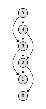
Hence
\begin{equation*} |V| = n + 1, \qquad |E| = 2(n-1) = 2n - 2 \quad (n \ge 1), \end{equation*}
and for \(n = 0\) the graph is a single vertex with no edges.
15.2 Matrix-chain multiplication
Determine an optimal parenthesization of a matrix-chain product \(A_1A_2\cdots A_6\) whose dimension sequence is \(\langle 5, 10, 3, 12, 5, 50, 6\rangle\).
The optimal parenthesization is \(((A_1A_2)((A_3A_4)(A_5A_6)))\), costing \(2010\) scalar multiplications (and it is the unique optimum). Running MATRIX-CHAIN-ORDER on \(p = \langle 5,10,3,12,5,50,6\rangle\) gives the following tables, with entry \(m[i,j]\) / \(s[i,j]\) in row \(i\), column \(j\):
| \(i \backslash j\) | 1 | 2 | 3 | 4 | 5 | 6 |
|---|---|---|---|---|---|---|
| 1 | 0 | 150 / 1 | 330 / 2 | 405 / 2 | 1655 / 4 | 2010 / 2 |
| 2 | 0 | 360 / 2 | 330 / 2 | 2430 / 2 | 1950 / 2 | |
| 3 | 0 | 180 / 3 | 930 / 4 | 1770 / 4 | ||
| 4 | 0 | 3000 / 4 | 1860 / 4 | |||
| 5 | 0 | 1500 / 5 | ||||
| 6 | 0 |
Reading off the splits: \(s[1,6]=2\), \(s[1,2]=1\), \(s[3,6]=4\), \(s[3,4]=3\), \(s[5,6]=5\). The cost is
\begin{equation*} \begin{aligned} m[1,6] &= m[1,2] + m[3,6] + p_0p_2p_6 = 150 + 1770 + 90 = 2010,\\ m[3,6] &= m[3,4] + m[5,6] + p_2p_4p_6 = 180 + 1500 + 90 = 1770 . \end{aligned} \end{equation*}
Write a recursive procedure MATRIX-CHAIN-MULTIPLY\((A, s, i, j)\) that really carries out the optimal matrix-chain multiplication. Its inputs are the matrix sequence \(A = \langle A_1, A_2, \ldots, A_n\rangle\), the table \(s\) produced by MATRIX-CHAIN-ORDER, and indices \(i\) and \(j\); the top-level call is MATRIX-CHAIN-MULTIPLY\((A, s, 1, n)\).
Split at \(k = s[i,j]\), recursively compute \(A_{i..k}\) and \(A_{k+1..j}\), and multiply the two results with the rectangular MATRIX-MULTIPLY of Section 15.2 (page 371).
MATRIX-CHAIN-MULTIPLY(A, s, i, j)
1  if i == j
2      return A[i]
3  k = s[i, j]
4  X = MATRIX-CHAIN-MULTIPLY(A, s, i, k)
5  Y = MATRIX-CHAIN-MULTIPLY(A, s, k + 1, j)
6  return MATRIX-MULTIPLY(X, Y)
Correctness, by induction on \(j - i\): if \(i = j\) the product \(A_{i..i}\) is \(A_i\). If \(i < j\), then \(i \le k < j\) by MATRIX-CHAIN-ORDER, so both recursive calls are on shorter chains and by the inductive hypothesis return \(X = A_{i..k}\) (a \(p_{i-1}\times p_k\) matrix) and \(Y = A_{k+1..j}\) (a \(p_k \times p_j\) matrix), each computed with an optimal parenthesization; these are compatible, and \(XY = A_{i..j}\). Since \(s[i,j]\) is a split achieving \(m[i,j] = m[i,k] + m[k+1,j] + p_{i-1}p_kp_j\), the multiplications performed number
\begin{equation*} m[i,k] + m[k+1,j] + p_{i-1}p_kp_j = m[i,j], \end{equation*}
which is optimal by (15.7).
Prove by the substitution method that the solution \(P(n)\) of recurrence (15.6), namely \(P(1) = 1\) and \(P(n) = \sum_{k=1}^{n-1} P(k)P(n-k)\) for \(n \ge 2\), satisfies \(P(n) = \Omega(2^n)\).
\(P(n) \ge \frac14 2^n\) for all \(n \ge 1\). The base cases are \(P(1) = 1 \ge 2^{-1}\) and \(P(2) = 1 \ge 2^0\). For \(n \ge 3\), assume \(P(k) \ge 2^{k-2}\) for \(1 \le k < n\); every term of (15.6) is positive and the terms \(k = 1\) and \(k = n-1\) are distinct, so
\begin{equation*} \begin{aligned} P(n) &\ge P(1)P(n-1) + P(n-1)P(1) = 2P(n-1)\\ &\ge 2 \cdot 2^{n-3} = 2^{n-2} = \tfrac14\, 2^n . \end{aligned} \end{equation*}
Hence \(P(n) = \Omega(2^n)\).
For matrix-chain multiplication on an input chain of length \(n\), describe the subproblem graph. How many vertices does it contain? How many edges does it contain, and which edges are they?
The graph has one vertex \((i,j)\) for each subchain \(A_iA_{i+1}\cdots A_j\) with \(1 \le i \le j \le n\), hence \(n(n+1)/2\) vertices, and an edge from \((i,j)\) to each of \((i,k)\) and \((k+1,j)\) for every \(i \le k < j\), hence \((n^3-n)/3\) edges.
By (15.7), solving \((i,j)\) with \(i < j\) directly consults \(m[i,k]\) and \(m[k+1,j]\) for each split \(k = i, \ldots, j-1\), and the vertices \((i,i)\) have no outgoing edges. The \(2(j-i)\) targets of \((i,j)\) are distinct: the \((i,k)\) differ in \(k\), the \((k+1,j)\) differ in \(k\), and \((i,k) = (k^{\prime}+1,j)\) would force \(k^{\prime} + 1 = i\), i.e. \(k^{\prime} < i\). Grouping vertices by \(d = j - i\) (there are \(n - d\) of them for each \(d\)),
\begin{equation*} \begin{aligned} |E| &= \sum_{d=0}^{n-1} (n-d)\cdot 2d = 2n\cdot\frac{(n-1)n}{2} - 2\cdot\frac{(n-1)n(2n-1)}{6}\\ &= n(n-1)\Bigl(n - \frac{2n-1}{3}\Bigr) = \frac{(n-1)n(n+1)}{3} = \frac{n^3-n}{3}. \end{aligned} \end{equation*}
Let \(R(i,j)\) count how many times the entry \(m[i,j]\) is referenced while MATRIX-CHAIN-ORDER computes other entries of the table. Prove that
\begin{equation*} \sum_{i=1}^{n}\sum_{j=i}^{n} R(i,j) = \frac{n^3-n}{3}. \end{equation*}
(Hint: equation (A.3) may help.)
\(R(i,j) = (n - j) + (i - 1)\), and summing this gives \((n^3-n)/3\).
The only references happen in line 10, which reads \(m[i^{\prime},k]\) and \(m[k+1,j^{\prime}]\) while computing \(m[i^{\prime},j^{\prime}]\), for each \(1 \le i^{\prime} \le k < j^{\prime} \le n\) (each triple is visited exactly once). So \(m[i,j]\) is read as the left operand once for each \(j^{\prime} \in \{j+1, \ldots, n\}\) (with \(i^{\prime} = i\), \(k = j\)), and as the right operand once for each \(i^{\prime} \in \{1, \ldots, i-1\}\) (with \(k = i - 1\), \(j^{\prime} = j\)). Grouping by \(d = j - i\) (with \(n - d\) pairs for each \(d\)) and substituting \(e = n - d\),
\begin{equation*} \begin{aligned} \sum_{i=1}^{n}\sum_{j=i}^{n} R(i,j) &= \sum_{d=0}^{n-1} (n-d)(n-1-d) = \sum_{e=1}^{n} e(e-1)\\ &= \frac{n(n+1)(2n+1)}{6} - \frac{n(n+1)}{2}\\ &= \frac{n(n+1)(n-1)}{3} = \frac{n^3-n}{3}, \end{aligned} \end{equation*}
using (A.3) for \(\sum e^2\) and (A.1) for \(\sum e\).
Prove that every full parenthesization of an expression with \(n\) elements uses exactly \(n-1\) pairs of parentheses.
By strong induction on \(n\), using the definition in Section 15.2 (a fully parenthesized product is a single element or a parenthesized product of two fully parenthesized products). If \(n = 1\) the expression is a single element, with \(0 = n-1\) pairs. If \(n \ge 2\) the expression is \((LR)\), where \(L\) is a full parenthesization of the first \(k\) elements and \(R\) of the remaining \(n-k\), for some \(1 \le k \le n-1\). Both are shorter, so by the inductive hypothesis the number of pairs is
\begin{equation*} 1 + (k-1) + (n-k-1) = n-1 . \end{equation*}
15.3 Elements of dynamic programming
To find the minimum number of scalar multiplications for a matrix chain \(A_1 A_2 \cdots A_n\), which is more efficient: listing every parenthesization of the product and evaluating the cost of each one, or running RECURSIVE-MATRIX-CHAIN? Justify your answer.
RECURSIVE-MATRIX-CHAIN is more efficient: it runs in \(O(n 3^n)\) time, while enumeration takes \(\Omega(4^n/n^{3/2})\) time.
Enumeration must look at all \(P(n)\) parenthesizations, and by Section 15.2 (recurrence (15.6) and Problem 12-4) \(P(n)\) is the Catalan number \(C_{n-1} = \Omega(4^n/n^{3/2})\), so its running time is \(\Omega(4^n/n^{3/2})\) (and actually \(\Theta(n)\) more per parenthesization to evaluate its cost).
For RECURSIVE-MATRIX-CHAIN on a chain of length \(n\), let \(N(n)\) be the number of calls it makes. A call on a chain of length \(1\) makes no further calls, and a call on a chain of length \(n \ge 2\) makes calls on chains of lengths \(k\) and \(n-k\) for each \(k = 1, \dots, n-1\), so
\begin{equation*} \begin{aligned} N(1) &= 1, \qquad N(n) = 1 + 2\sum_{k=1}^{n-1} N(k) \quad (n \ge 2),\\ N(n) - N(n-1) &= 2N(n-1) \quad (n \ge 3), \qquad N(2) = 3, \end{aligned} \end{equation*}
so \(N(n) = 3^{n-1}\). Outside its recursive calls, each call does \(O(n)\) work (one loop of at most \(n-1\) constant-time iterations), so the total running time is
\begin{equation*} T(n) = O(n \cdot 3^{n-1}) = O(n 3^n). \end{equation*}
Since
\begin{equation*} \frac{4^n/n^{3/2}}{n 3^n} = \frac{(4/3)^n}{n^{5/2}} \to \infty, \end{equation*}
the recursive procedure is asymptotically faster.
Draw the recursion tree of the MERGE-SORT procedure of Section 2.3.1 when it sorts an array of 16 elements. Explain why memoization does not speed up a good divide-and-conquer algorithm like MERGE-SORT.
The tree is the complete binary tree of depth 4 below; each node is the call MERGE-SORT(A, p, r), labelled by its index range \(p..r\), and the call on \(p..r\) with \(p < r\) has children \(p..q\) and \(q+1..r\), \(q = \lfloor (p+r)/2 \rfloor\).
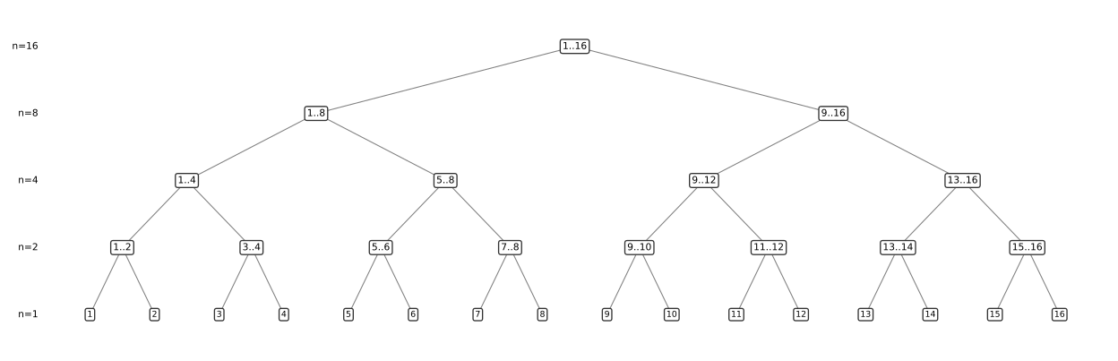
Memoization fails because the subproblems do not overlap: all \(31\) calls are on distinct ranges. Indeed, the ranges at depth \(d\) have length \(16/2^d\) and partition \(1..16\), so two calls at the same depth have disjoint ranges, and two calls at different depths have ranges of different lengths. Hence no call ever finds its answer already in the memo table; memoization only adds table overhead. In general, a good divide-and-conquer algorithm generates brand-new subproblems at every step, whereas memoization pays off only when subproblems overlap (Section 15.3).
Consider the variant of matrix-chain multiplication in which we want a parenthesization of \(A_1 A_2 \cdots A_n\) that maximizes, instead of minimizes, the number of scalar multiplications. Does this problem have optimal substructure?
Yes. Let \(M[i,j]\) be the maximum cost of a parenthesization of \(A_i \cdots A_j\); then
\begin{equation*} M[i,i] = 0, \qquad M[i,j] = \max_{i \le k < j} \bigl( M[i,k] + M[k+1,j] + p_{i-1} p_k p_j \bigr) \quad (i < j). \end{equation*}
The cut-and-paste argument of Section 15.2 (step 1) goes through verbatim with the inequality reversed. Suppose an optimal (maximum-cost) parenthesization of \(A_i \cdots A_j\), \(i < j\), splits between \(A_k\) and \(A_{k+1}\). Its cost is
\begin{equation*} (\text{cost of its } A_i \cdots A_k \text{ part}) + (\text{cost of its } A_{k+1} \cdots A_j \text{ part}) + p_{i-1} p_k p_j , \end{equation*}
and the two parts can be chosen independently, since each is just some parenthesization of its own subchain and the last term depends only on \(k\). If the \(A_i \cdots A_k\) part did not have the maximum cost \(M[i,k]\), swapping in a costlier parenthesization of \(A_i \cdots A_k\) would give a costlier parenthesization of \(A_i \cdots A_j\), a contradiction; the same goes for \(A_{k+1} \cdots A_j\). So an optimal solution is made of optimal solutions to the two subproblems, and the recurrence holds.
Dynamic programming solves the subproblems first and only then decides which of them an optimal solution uses. Professor Capulet argues that solving all the subproblems is not always necessary: for matrix-chain multiplication she proposes to choose the split point \(A_k\) of each subproduct \(A_i A_{i+1} \cdots A_j\) greedily, by picking the \(k\) that minimizes \(p_{i-1} p_k p_j\), before solving any subproblems. Give an instance of matrix-chain multiplication on which this greedy method produces a suboptimal parenthesization.
Take three matrices with dimension sequence \(\langle p_0, p_1, p_2, p_3 \rangle = \langle 1, 2, 3, 4 \rangle\), so \(A_1\) is \(1 \times 2\), \(A_2\) is \(2 \times 3\), \(A_3\) is \(3 \times 4\).
For the whole chain the greedy rule compares \(p_0 p_1 p_3 = 8\) (\(k = 1\)) with \(p_0 p_2 p_3 = 12\) (\(k = 2\)) and splits at \(k = 1\), giving \(A_1 (A_2 A_3)\); the remaining subchains have only one way to be multiplied. The two parenthesizations cost
\begin{equation*} \begin{aligned} A_1 (A_2 A_3) &: \; p_1 p_2 p_3 + p_0 p_1 p_3 = 24 + 8 = 32,\\ (A_1 A_2) A_3 &: \; p_0 p_1 p_2 + p_0 p_2 p_3 = 6 + 12 = 18, \end{aligned} \end{equation*}
so the greedy answer \(32\) exceeds the optimum \(18\).
In the rod-cutting problem of Section 15.1, suppose that in addition we may produce at most \(l_i\) pieces of length \(i\), for \(i = 1, 2, \dots, n\). Show that the optimal-substructure property described in Section 15.1 then fails.
Take \(n = 4\), prices \(p_1 = 1\), \(p_2 = 5\), \(p_3 = 5\), \(p_4 = 1\), and limits \(l_1 = 4\), \(l_2 = l_3 = l_4 = 1\) (only the length-2 limit matters). The feasible ways to cut the rod of length \(4\) and their revenues are
| cuts | \(4\) | \(3+1\) | \(2+1+1\) | \(1+1+1+1\) | \(2+2\) |
|---|---|---|---|---|---|
| revenue | \(1\) | \(6\) | \(7\) | \(4\) | infeasible |
so the unique optimal solution is \(2 + 1 + 1\), with \(r_4 = 7\); similarly \(r_2 = 5\) (leave it uncut) and \(r_3 = 6\).
The property of Section 15.1 says that an optimal solution which first cuts off a piece of length \(i\) consists of that piece plus an optimal solution of the remaining rod of length \(n - i\), giving recurrence (15.2), \(r_n = \max_{1 \le i \le n} (p_i + r_{n-i})\). Both fail here: (i) the optimal solution \(2 + 1 + 1\) cuts off a piece of length \(2\), but its remainder \(1 + 1\) earns \(2 < 5 = r_2\), so it is not an optimal solution of the length-2 subproblem; (ii) the recurrence gives \(\max(p_1 + r_3, p_2 + r_2, p_3 + r_1, p_4 + r_0) = \max(7, 10, 6, 1) = 10 \ne 7 = r_4\), since the value \(p_2 + r_2 = 10\) belongs to the infeasible cut \(2 + 2\).
You want to convert currency 1 into currency \(n\), among \(n\) currencies numbered \(1, 2, \dots, n\), possibly via a chain of trades through intermediate currencies. For each pair \(i, j\) there is an exchange rate \(r_{ij}\): \(d\) units of currency \(i\) trade for \(d r_{ij}\) units of currency \(j\). A sequence of trades may carry a commission depending only on how many trades it uses; \(c_k\) is the commission for a sequence of \(k\) trades. Show that if \(c_k = 0\) for all \(k = 1, 2, \dots, n\), then finding the best sequence of exchanges from currency 1 to currency \(n\) has optimal substructure. Then show that for arbitrary commissions \(c_k\) the problem need not have optimal substructure.
Rates are positive, we start with \(1\) unit of currency \(1\), and a sequence \(1 = a_0, a_1, \dots, a_k\) of \(k\) trades ending in currency \(a_k\) is worth
\begin{equation*} \mathrm{val}(a_0, \dots, a_k) = r_{a_0 a_1} r_{a_1 a_2} \cdots r_{a_{k-1} a_k} - c_k \end{equation*}
units of \(a_k\). A best sequence from currency \(s\) to currency \(t\) is one of maximum value (we assume it exists, as it does when no cycle of trades has rate product above \(1\)).
No commissions. Let \(S = (1 = a_0, \dots, a_k = n)\) be a best sequence from \(1\) to \(n\), and split it at any intermediate currency \(j = a_m\) into \(S_1 = (a_0, \dots, a_m)\) and \(S_2 = (a_m, \dots, a_k)\). With \(c \equiv 0\), \(\mathrm{val}(S) = \mathrm{val}(S_1)\,\mathrm{val}(S_2)\). If some sequence \(S_1^{\prime}\) from \(1\) to \(j\) had \(\mathrm{val}(S_1^{\prime}) > \mathrm{val}(S_1)\), then \(S_1^{\prime}\) followed by \(S_2\) is a sequence from \(1\) to \(n\) with
\begin{equation*} \mathrm{val}(S_1^{\prime})\,\mathrm{val}(S_2) > \mathrm{val}(S_1)\,\mathrm{val}(S_2) = \mathrm{val}(S), \end{equation*}
contradicting optimality of \(S\) (using \(\mathrm{val}(S_2) > 0\)). Likewise \(S_2\) is a best sequence from \(j\) to \(n\). So an optimal solution contains optimal solutions to the subproblems (best \(1 \to j\) and \(j \to n\) sequences), which can be solved independently.
Arbitrary commissions. Take \(n = 3\) with
\begin{equation*} \begin{aligned} &r_{12} = 2, \quad r_{23} = 2, \quad r_{13} = 3, \quad r_{21} = r_{32} = \tfrac14, \quad r_{31} = \tfrac18,\\ &c_1 = 2, \qquad c_k = 0 \quad (k \ge 2). \end{aligned} \end{equation*}
The simple cycles have rate products \(r_{12} r_{21} = r_{23} r_{32} = r_{12} r_{23} r_{31} = \tfrac12\), \(r_{13} r_{31} = \tfrac38\) and \(r_{13} r_{32} r_{21} = \tfrac{3}{16}\), all at most \(\tfrac12\). The only cycle-free sequences from \(1\) to \(3\) are \((1,3)\), worth \(3 - 2 = 1\), and \((1,2,3)\), worth \(4 - 0 = 4\). Every other sequence from \(1\) to \(3\) is a cycle-free one plus at least one cycle, so it has at least \(2\) trades and is worth at most \(4 \cdot \tfrac12 = 2\). Hence \((1,2,3)\) is the unique best sequence, with value \(4\). But its pieces are not best for their subproblems: (i) the prefix \((1,2)\) is worth \(2 - c_1 = 0\), while \((1,3,2)\) is worth \(3 \cdot \tfrac14 - c_2 = \tfrac34\); (ii) the suffix \((2,3)\) is worth \(2 - c_1 = 0\), while \((2,1,3)\) is worth \(\tfrac14 \cdot 3 - c_2 = \tfrac34\). So with commissions the best sequence need not contain best subsequences: optimal substructure fails.
15.4 Longest common subsequence
Find a longest common subsequence of \(X = \langle 1,0,0,1,0,1,0,1\rangle\) and \(Y = \langle 0,1,0,1,1,0,1,1,0\rangle\).
An LCS is \(\langle 1,0,0,1,1,0\rangle\), of length \(6\).
Running LCS-LENGTH on \(X\) (rows \(i = 0,\dots,8\)) and \(Y\) (columns \(j = 0,\dots,9\)) fills the \(c\) table by equation (15.9):
| \(i \backslash j\) | 0 | 1 | 2 | 3 | 4 | 5 | 6 | 7 | 8 | 9 |
|---|---|---|---|---|---|---|---|---|---|---|
| \(0\) | 0 | 0 | 0 | 0 | 0 | 0 | 0 | 0 | 0 | 0 |
| \(1\) (\(x_1 = 1\)) | 0 | 0 | 1 | 1 | 1 | 1 | 1 | 1 | 1 | 1 |
| \(2\) (\(x_2 = 0\)) | 0 | 1 | 1 | 2 | 2 | 2 | 2 | 2 | 2 | 2 |
| \(3\) (\(x_3 = 0\)) | 0 | 1 | 1 | 2 | 2 | 2 | 3 | 3 | 3 | 3 |
| \(4\) (\(x_4 = 1\)) | 0 | 1 | 2 | 2 | 3 | 3 | 3 | 4 | 4 | 4 |
| \(5\) (\(x_5 = 0\)) | 0 | 1 | 2 | 3 | 3 | 3 | 4 | 4 | 4 | 5 |
| \(6\) (\(x_6 = 1\)) | 0 | 1 | 2 | 3 | 4 | 4 | 4 | 5 | 5 | 5 |
| \(7\) (\(x_7 = 0\)) | 0 | 1 | 2 | 3 | 4 | 4 | 5 | 5 | 5 | 6 |
| \(8\) (\(x_8 = 1\)) | 0 | 1 | 2 | 3 | 4 | 5 | 5 | 6 | 6 | 6 |
so the LCS length is \(c[8,9] = 6\). Tracing back from \((8,9)\) as PRINT-LCS does (moving up on ties) yields \(\langle 1,0,0,1,1,0\rangle\), which occurs in \(X\) at positions \(1,2,3,4,6,7\) and in \(Y\) at positions \(2,3,6,7,8,9\).
Write pseudocode that, given the completed \(c\) table and the original sequences \(X = \langle x_1,x_2,\dots,x_m\rangle\) and \(Y = \langle y_1,y_2,\dots,y_n\rangle\), reconstructs an LCS in \(O(m+n)\) time without consulting the \(b\) table.
Retrace PRINT-LCS, but decide each step from \(X\), \(Y\) and two neighbouring \(c\) entries instead of reading \(b[i,j]\); the initial call is PRINT-LCS-C\((c,X,Y,m,n)\).
PRINT-LCS-C(c, X, Y, i, j)
1  if i == 0 or j == 0
2      return
3  if x_i == y_j
4      PRINT-LCS-C(c, X, Y, i - 1, j - 1)
5      print x_i
6  elseif c[i - 1, j] >= c[i, j - 1]
7      PRINT-LCS-C(c, X, Y, i - 1, j)
8  else PRINT-LCS-C(c, X, Y, i, j - 1)
Correctness, by induction on \(i + j\): the call on \((i,j)\) prints an LCS of \(X_i\) and \(Y_j\). For \(i = 0\) or \(j = 0\) the LCS is empty. If \(x_i = y_j\), then \(c[i,j] = c[i-1,j-1] + 1\) by (15.9), and an LCS of \(X_{i-1}, Y_{j-1}\) (printed by line 4, by induction) followed by \(x_i\) is a common subsequence of \(X_i, Y_j\) of length \(c[i,j]\), hence an LCS. If \(x_i \ne y_j\), then by (15.9)
\begin{equation*} c[i,j] = \max(c[i-1,j],\, c[i,j-1]), \end{equation*}
and line 6 recurses into the prefix pair attaining the maximum, whose LCS (by induction) is a common subsequence of \(X_i, Y_j\) of length \(c[i,j]\).
Each call does \(O(1)\) work besides at most one recursive call, and every recursive call decreases \(i + j\) by at least \(1\), so there are at most \(m + n + 1\) calls and the running time is \(O(m+n)\).
Write a memoized version of LCS-LENGTH whose running time is \(O(mn)\).
Evaluate recurrence (15.9) top-down, caching each \(c[i,j]\) the first time it is computed (the pattern of MEMOIZED-CUT-ROD in Section 15.1), with \(-1\) marking an unknown entry.
MEMOIZED-LCS-LENGTH(X, Y)
1  m = X.length,  n = Y.length
2  let c[0..m, 0..n] be a new table
3  for i = 0 to m
4      for j = 0 to n
5          c[i, j] = -1
6  return LOOKUP-LCS(c, X, Y, m, n)

LOOKUP-LCS(c, X, Y, i, j)
1  if c[i, j] > -1
2      return c[i, j]
3  if i == 0 or j == 0
4      c[i, j] = 0
5  elseif x_i == y_j
6      c[i, j] = LOOKUP-LCS(c, X, Y, i - 1, j - 1) + 1
7  else c[i, j] = max(LOOKUP-LCS(c, X, Y, i - 1, j),
                      LOOKUP-LCS(c, X, Y, i, j - 1))
8  return c[i, j]
Correctness: by induction on \(i + j\), LOOKUP-LCS\((c,X,Y,i,j)\) returns the LCS length of \(X_i, Y_j\), since lines 3–7 are exactly the three cases of (15.9) applied to correct values for smaller \(i + j\), and an entry is cached only after it has been computed correctly.
Running time: initialization takes \(\Theta(mn)\). For each \((i,j)\), lines 3–8 run at most once, because afterwards \(c[i,j] \ge 0\) and every later call returns at line 2; each such run makes at most \(2\) recursive calls. Hence the number of calls is at most \(1 + 2(m+1)(n+1)\), each costing \(O(1)\) apart from its recursive calls, for \(O(mn)\) in total.
Explain how to compute the length of an LCS while storing only \(2\cdot\min(m,n)\) entries of the \(c\) table plus \(O(1)\) additional space. Then explain how to achieve the same using only \(\min(m,n)\) table entries plus \(O(1)\) additional space.
Since an LCS of \(X, Y\) is an LCS of \(Y, X\), swap the sequences if necessary so that \(n = \min(m,n)\) is the length of \(Y\), which indexes the columns; and since \(c[i,0] = c[0,j] = 0\), column \(0\) and row \(0\) need not be stored. By (15.9), row \(i\) of \(c\) depends only on row \(i-1\) and on entries of row \(i\) to its left.
Two rows (\(2n\) entries). Keep arrays \(P[1..n]\) (row \(i-1\)) and \(C[1..n]\) (row \(i\)), reading \(P[0] = C[0] = 0\). For \(i = 1,\dots,m\) fill \(C[j]\) for \(j = 1,\dots,n\) by
\begin{equation*} C[j] = \begin{cases} P[j-1] + 1 & \text{if } x_i = y_j, \\ \max(P[j],\, C[j-1]) & \text{otherwise,} \end{cases} \end{equation*}
then exchange the roles of \(P\) and \(C\) (swap two pointers, or index rows by \(i \bmod 2\)). After row \(m\) the answer is \(c[m,n]\), held in the last-written row (it is \(0\) if \(n = 0\)). Extra space: the indices \(i, j\) and the pointers, \(O(1)\).
One row (\(n\) entries). Overwrite a single array in place, keeping in two scalars the only entries that would otherwise be lost: \(diag = c[i-1,j-1]\) and \(left = c[i,j-1]\).
LCS-LENGTH-ONE-ROW(X, Y)        // assumes n <= m; else swap X and Y
1  m = X.length,  n = Y.length
2  if n == 0
3      return 0
4  let c[1..n] be a new array, with every entry 0
5  for i = 1 to m
6      diag = 0,  left = 0         // c[i-1, 0] and c[i, 0]
7      for j = 1 to n
8          up = c[j]               // c[i-1, j]
9          if x_i == y_j
10             c[j] = diag + 1
11         else c[j] = max(up, left)
12         diag = up,  left = c[j]
13 return c[n]
Loop invariant of the inner loop (for fixed \(i\)): at the start of iteration \(j\), \(c[1..j-1]\) hold \(c[i,1..j-1]\), \(c[j..n]\) hold \(c[i-1,j..n]\), \(diag = c[i-1,j-1]\) and \(left = c[i,j-1]\). Initialization: before \(j = 1\) the array is row \(i-1\) (row \(0\) is all zeros, set in line 4) and line 6 sets the two boundary zeros. Maintenance: line 8 reads \(c[i-1,j]\) before it is overwritten, lines 9–11 are (15.9), and line 12 shifts \(diag\) to \(c[i-1,j]\) and \(left\) to \(c[i,j]\). Termination: after \(j = n\) the array holds row \(i\), which is the outer loop’s invariant for \(i+1\); after \(i = m\), \(c[n] = c[m,n]\).
Both versions take \(\Theta(mn)\) time, like LCS-LENGTH, and use \(2\min(m,n)\) resp. \(\min(m,n)\) table entries plus the \(O(1)\) scalars \(i, j, diag, left, up\).
Design an \(O(n^2)\)-time algorithm that finds a longest monotonically increasing subsequence of a given sequence of \(n\) numbers.
Let \(L[i]\) be the length of a longest monotonically increasing subsequence ending at \(A[i]\); then
\begin{equation*} L[i] = 1 + \max\{\, L[k] : 1 \le k < i,\ A[k] \le A[i] \,\} \end{equation*}
(with \(\max \emptyset = 0\)), the answer is \(\max_i L[i]\), and a predecessor array \(p\) recovers the subsequence. Monotonically increasing means \(\le\) between consecutive terms, as in Section 3.2.
LIS(A, n)                          // n >= 1
1  let L[1..n] and p[1..n] be new arrays
2  for i = 1 to n
3      L[i] = 1,  p[i] = NIL
4      for k = 1 to i - 1
5          if A[k] <= A[i] and L[k] + 1 > L[i]
6              L[i] = L[k] + 1,  p[i] = k
7  best = 1
8  for i = 2 to n
9      if L[i] > L[best]
10         best = i
11 PRINT-LIS(A, p, best)

PRINT-LIS(A, p, i)
1  if i != NIL
2      PRINT-LIS(A, p, p[i])
3      print A[i]
Correctness, by induction on \(i\): after iteration \(i\) of line 2, \(L[i]\) is the recurrence’s value and following \(p\) from \(i\) lists an increasing subsequence of that length ending at \(A[i]\). The recurrence is right: deleting \(A[i]\) from a longest increasing subsequence ending at \(A[i]\) (of length at least \(2\)) leaves one ending at some \(A[k]\) with \(k < i\) and \(A[k] \le A[i]\), of length at most \(L[k]\); conversely appending \(A[i]\) to the subsequence recorded for any such \(k\) gives length \(L[k] + 1\). Every increasing subsequence ends at some index, so the one printed from \(best\) is longest.
Running time: lines 4–6 run \(\sum_{i=1}^{n} (i-1) = n(n-1)/2\) times at \(O(1)\) each, and lines 7–11 cost \(O(n)\), for \(O(n^2)\) in total.
(Starred.) Design an \(O(n \lg n)\)-time algorithm that finds a longest monotonically increasing subsequence of a given sequence of \(n\) numbers. Hint: the last element of a candidate subsequence of length \(i\) is at least as large as the last element of a candidate subsequence of length \(i-1\); maintain the candidate subsequences by linking them through the input sequence.
Scan \(A\) left to right, keeping for each length \(\ell\) the index \(M[\ell]\) of the smallest possible last element of an increasing subsequence of length \(\ell\) seen so far; these last elements are sorted, so each \(A[i]\) is placed by binary search, and predecessor links \(p[i]\) thread the candidates through \(A\). As in Exercise 15.4-5, increasing means \(\le\) between consecutive terms.
LIS-FAST(A, n)                     // n >= 1
1  let M[1..n] and p[1..n] be new arrays
2  len = 0
3  for i = 1 to n
4      lo = 1,  hi = len + 1       // least l <= len with A[M[l]] > A[i],
5      while lo < hi               //   or len + 1 if there is none
6          mid = floor((lo + hi) / 2)
7          if A[M[mid]] > A[i]
8              hi = mid
9          else lo = mid + 1
10     if lo > 1
11         p[i] = M[lo - 1]
12     else p[i] = NIL
13     M[lo] = i
14     len = max(len, lo)
15 PRINT-LIS(A, p, M[len])         // PRINT-LIS from Exercise 15.4-5
For the prefix \(A[1..i]\) let \(\lambda_i\) be its LIS length and, for \(1 \le \ell \le \lambda_i\), let \(t_\ell\) be the least last value of an increasing subsequence of length \(\ell\) in it (\(t_\ell = \infty\) for \(\ell > \lambda_i\)). Then \(t_{\ell-1} \le t_\ell\): the first \(\ell-1\) terms of a length-\(\ell\) subsequence ending in \(t_\ell\) end in a value \(\le t_\ell\). Loop invariant at the start of iteration \(i\) (for the prefix \(A[1..i-1]\)): \(len = \lambda_{i-1}\), \(A[M[\ell]] = t_\ell\) for \(\ell \le len\), and following \(p\) from \(M[\ell]\) lists an increasing subsequence of length \(\ell\) ending at index \(M[\ell]\).
Initialization: \(len = 0\), vacuous. Maintenance: since \(A[M[1..len]]\) is sorted, the predicate \(A[M[\ell]] > A[i]\) is monotone in \(\ell\), so lines 4–9 find \(\ell^* = \min\{\ell : t_\ell > A[i]\}\) (accessing only \(mid < hi \le len + 1\)). A length-\(\ell\) subsequence of \(A[1..i]\) either avoids \(i\) or ends at \(i\), and the latter is possible iff \(\ell = 1\) or \(t_{\ell-1} \le A[i]\). Hence the new values \(t^{\prime}_\ell\) are: (i) \(\ell < \ell^*\): \(t_\ell \le A[i]\), so \(t^{\prime}_\ell = \min(t_\ell, A[i]) = t_\ell\), and \(M[\ell]\) is kept; (ii) \(\ell = \ell^*\): \(t_{\ell-1} \le A[i] < t_\ell\), so \(t^{\prime}_\ell = A[i]\), which line 13 records, with chain \(p[i] = M[\ell^*-1]\) of length \(\ell^* - 1\) ending at a value \(\le A[i]\), extended by \(i\); (iii) \(\ell > \ell^*\): \(t_{\ell-1} \ge t_{\ell^*} > A[i]\), so \(t^{\prime}_\ell = t_\ell\), kept. In particular \(\lambda_i = len + 1\) iff \(\ell^* = len + 1\), matching line 14, and old links \(p[k]\) never change, so old chains stay valid. Termination: \(len = \lambda_n\) and the chain from \(M[len]\) is an increasing subsequence of that length, which line 15 prints.
Running time: each binary search is over at most \(len + 1 \le n\) positions and takes \(O(\lg n)\) iterations; everything else in an iteration of line 3 is \(O(1)\), and line 15 costs \(O(n)\). The total is \(O(n \lg n)\).
15.5 Optimal binary search trees
Give pseudocode for a procedure CONSTRUCT-OPTIMAL-BST\((root)\) that takes the table \(root\) produced by OPTIMAL-BST and prints the structure of an optimal binary search tree. On the tables of Figure 15.10 (keys \(k_1,\dots,k_5\), dummy keys \(d_0,\dots,d_5\)) it should print the eleven lines \(k_2\) is the root; \(k_1\) is the left child of \(k_2\); \(d_0\) is the left child of \(k_1\); \(d_1\) is the right child of \(k_1\); \(k_5\) is the right child of \(k_2\); \(k_4\) is the left child of \(k_5\); \(k_3\) is the left child of \(k_4\); \(d_2\) is the left child of \(k_3\); \(d_3\) is the right child of \(k_3\); \(d_4\) is the right child of \(k_4\); \(d_5\) is the right child of \(k_5\), which describe the optimal tree of Figure 15.9(b).
Print \(k_r\) with \(r = root[1,n]\) as the root, then recursively describe the subtree on keys \(k_i,\dots,k_j\) hanging off a given parent and side: if \(j = i-1\) it is the single leaf \(d_j\), otherwise its root is \(k_{root[i,j]}\) and we recurse on both sides of it (preorder).
CONSTRUCT-OPTIMAL-BST(root)
1  n = root.rows
2  r = root[1, n]
3  print "k" r " is the root"
4  CONSTRUCT-SUBTREE(root, 1, r - 1, r, "left")
5  CONSTRUCT-SUBTREE(root, r + 1, n, r, "right")

CONSTRUCT-SUBTREE(root, i, j, parent, side)
1  if j == i - 1
2      print "d" j " is the " side " child of k" parent
3  else r = root[i, j]
4      print "k" r " is the " side " child of k" parent
5      CONSTRUCT-SUBTREE(root, i, r - 1, r, "left")
6      CONSTRUCT-SUBTREE(root, r + 1, j, r, "right")
Correctness, by induction on \(j-i\): the subtree containing keys \(k_i,\dots,k_j\) has leaves \(d_{i-1},\dots,d_j\). If \(j=i-1\) this is just \(d_{i-1}=d_j\), printed in line 2. If \(j \ge i\), by the definition of \(root[i,j]\) (Section 15.5, after (15.14)) its root is \(k_r\) with \(r=root[i,j]\), its left subtree contains \(k_i,\dots,k_{r-1}\) and its right subtree \(k_{r+1},\dots,k_j\), and the two recursive calls describe these correctly by the inductive hypothesis (both have smaller \(j-i\)). CONSTRUCT-OPTIMAL-BST applies the same step to \([1,n]\). Running it on the \(root\) table of Figure 15.10 prints exactly the eleven lines above, in that order.
Find the expected search cost and the shape of an optimal binary search tree on \(n = 7\) keys whose probabilities are
| \(i\) | 0 | 1 | 2 | 3 | 4 | 5 | 6 | 7 |
|---|---|---|---|---|---|---|---|---|
| \(p_i\) | 0.04 | 0.06 | 0.08 | 0.02 | 0.10 | 0.12 | 0.14 | |
| \(q_i\) | 0.06 | 0.06 | 0.06 | 0.06 | 0.05 | 0.05 | 0.05 | 0.05 |
The optimal expected cost is \(e[1,7] = 3.12\), attained by the tree with root \(k_5\), left subtree \(k_2(k_1,\,k_3(\,\cdot\,,k_4))\) and right subtree \(k_7(k_6,\,\cdot\,)\); it is the unique optimum.
Running OPTIMAL-BST gives the table \(root[i,j]\) (row \(i\), column \(j\)):
| \(i \backslash j\) | 1 | 2 | 3 | 4 | 5 | 6 | 7 |
|---|---|---|---|---|---|---|---|
| 1 | 1 | 2 | 2 | 2 | 3 | 3 | 5 |
| 2 | 2 | 3 | 3 | 3 | 5 | 5 | |
| 3 | 3 | 3 | 4 | 5 | 5 | ||
| 4 | 4 | 5 | 5 | 6 | |||
| 5 | 5 | 6 | 6 | ||||
| 6 | 6 | 7 | |||||
| 7 | 7 |
and first row of \(e\): \(e[1,1..7] = 0.28,\ 0.62,\ 1.02,\ 1.34,\ 1.83,\ 2.44,\ 3.12\). CONSTRUCT-OPTIMAL-BST (Exercise 15.5-1) then reads off the tree:
- \(k_5\) is the root; \(k_2\) is its left child and \(k_7\) its right child;
- \(k_1\) is the left child of \(k_2\), with leaves \(d_0, d_1\);
- \(k_3\) is the right child of \(k_2\), with left leaf \(d_2\) and right child \(k_4\), whose leaves are \(d_3, d_4\);
- \(k_6\) is the left child of \(k_7\), with leaves \(d_5, d_6\); \(d_7\) is the right child of \(k_7\).
Check against (15.11), summing \((\mathrm{depth}+1)\) times the probability:
\begin{equation*} \begin{aligned} \textstyle\sum_i (\mathrm{depth}(k_i)+1)p_i &= 0.10 + 2(0.06+0.14) + 3(0.04+0.08+0.12) + 4(0.02)\\ &= 1.30,\\ \textstyle\sum_i (\mathrm{depth}(d_i)+1)q_i &= 3(0.05) + 4(0.06+0.06+0.06+0.05+0.05) + 5(0.06+0.05)\\ &= 1.82, \end{aligned} \end{equation*}
total \(3.12\). An exhaustive check of all \(429\) binary search trees on 7 keys confirms that no other tree attains \(3.12\).
Suppose OPTIMAL-BST drops the table \(w[i,j]\): in line 9 it instead evaluates \(w(i,j)\) directly from the sum (15.12), and line 11 uses that freshly computed value. What happens to the asymptotic running time?
Nothing: the running time stays \(\Theta(n^3)\).
Evaluating (15.12) for a pair \(i \le j\) adds \((j-i+1) + (j-i+2)\) probabilities, i.e. costs \(\Theta(j-i+1)\), and line 9 runs once per pair \((i,j)\), outside the loop of lines 10–14. That loop already performs \(j-i+1\) iterations of \(\Theta(1)\) work for the same pair, so the cost of handling the pair changes from \(\Theta(j-i+1)\) to \(\Theta(j-i+1)+\Theta(j-i+1)=\Theta(j-i+1)\). Summing over all pairs,
\begin{equation*} \begin{aligned} \sum_{l=1}^{n}\ \sum_{i=1}^{n-l+1} \Theta(l) &= \Theta\Bigl(\sum_{l=1}^{n} l\,(n-l+1)\Bigr)\\ &= \Theta\Bigl(\frac{n(n+1)(n+2)}{6}\Bigr) = \Theta(n^3), \end{aligned} \end{equation*}
the same bound the book derives for the original procedure.
Knuth [212] proved that roots of optimal subtrees can always be chosen so that \(root[i,j-1] \le root[i,j] \le root[i+1,j]\) whenever \(1 \le i < j \le n\). Using this fact, modify OPTIMAL-BST so that it runs in \(\Theta(n^2)\) time.
Restrict the candidate roots for \(e[i,j]\), \(i<j\), to \(root[i,j-1] \le r \le root[i+1,j]\) instead of \(i \le r \le j\); the telescoping range lengths make each diagonal cost \(O(n)\).
KNUTH-OPTIMAL-BST(p, q, n)
 1  let e[1..n+1, 0..n], w[1..n+1, 0..n], root[1..n, 1..n] be new tables
 2  for i = 1 to n + 1
 3      e[i, i - 1] = q[i - 1]
 4      w[i, i - 1] = q[i - 1]
 5  for i = 1 to n
 6      w[i, i] = w[i, i - 1] + p[i] + q[i]
 7      e[i, i] = e[i, i - 1] + e[i + 1, i] + w[i, i]
 8      root[i, i] = i
 9  for l = 2 to n
10      for i = 1 to n - l + 1
11          j = i + l - 1
12          e[i, j] = infinity
13          w[i, j] = w[i, j - 1] + p[j] + q[j]
14          for r = root[i, j - 1] to root[i + 1, j]
15              t = e[i, r - 1] + e[r + 1, j] + w[i, j]
16              if t < e[i, j]
17                  e[i, j] = t
18                  root[i, j] = r
19  return e and root
Correctness. We use Knuth’s fact in the form he proves it, for the leftmost optimal roots: if \(R(i,j)\) denotes the smallest \(r\) attaining the minimum in (15.14), then \(R(i,j-1) \le R(i,j) \le R(i+1,j)\). Claim, by induction on \(l=j-i+1\): the procedure sets \(e[i,j]\) to the value (15.14) and \(root[i,j]=R(i,j)\). For \(l=1\) the only candidate is \(r=i\) (lines 5–8). For \(l \ge 2\), lines 9–11 process diagonal \(l\) after diagonal \(l-1\), so by the hypothesis \(root[i,j-1]=R(i,j-1)\) and \(root[i+1,j]=R(i+1,j)\); hence the loop of line 14 ranges over a nonempty subset of \(\{i,\dots,j\}\) (since \(i \le R(i,j-1) \le R(i+1,j) \le j\)) that contains \(R(i,j)\). Every value \(t\) it sees is one of the terms minimized in (15.14), so it finds the true minimum; and because the test in line 16 is strict and \(R(i,j)\) is the leftmost minimizer overall, no earlier \(r\) in the range ties it, so \(root[i,j]=R(i,j)\).
Running time. Lines 1–8 take \(\Theta(n)\) apart from allocating the tables. For a fixed \(l \ge 2\) the loop of line 14 does \(root[i+1,i+l-1]-root[i,i+l-2]+1\) iterations for row \(i\), and summing over \(i\) telescopes:
\begin{equation*} \begin{aligned} \sum_{i=1}^{n-l+1}\bigl(root[i+1,i+l-1]-root[i,i+l-2]+1\bigr) &= root[n-l+2,n]-root[1,l-1]+(n-l+1)\\ &\le n + n = O(n). \end{aligned} \end{equation*}
So each of the \(n-1\) diagonals costs \(O(n)\), for \(O(n^2)\) in total; since the procedure fills \(\Theta(n^2)\) table entries, the running time is \(\Theta(n^2)\).
Problems for Chapter 15
Longest simple path in a directed acyclic graph: A directed acyclic graph \(G = (V, E)\) is given, together with real-valued edge weights \(w\) and two distinguished vertices \(s\) and \(t\). Describe a dynamic-programming method that finds a longest weighted simple path from \(s\) to \(t\). Describe the subproblem graph, and state the efficiency of your algorithm.
Let \(d(v)\) be the weight of a longest path from \(s\) to \(v\) (\(-\infty\) if none); then \(d(s) = 0\) and
\begin{equation*} d(v) = \max_{(u,v) \in E} \bigl( d(u) + w(u,v) \bigr) \quad (v \ne s), \end{equation*}
evaluated in topological order, in \(\Theta(V + E)\) time; the answer is \(d(t)\), recovered via predecessor pointers.
Since \(G\) is acyclic, every path is simple (a repeated vertex would close a cycle), so the simplicity constraint that defeats optimal substructure in the longest-simple-path discussion of Section 15.3 is vacuous here. Optimal substructure then holds by cut-and-paste: if \(p\) is a longest \(s \leadsto v\) path with last edge \((u,v)\), its prefix \(p^{\prime}\) is a longest \(s \leadsto u\) path, for a heavier \(s \leadsto u\) path \(p^{\prime\prime}\) would give the heavier path \(p^{\prime\prime} \to v\), which is again a path because \(G\) is acyclic. This justifies the recurrence. The bottom-up procedure is DAG-SHORTEST-PATHS (Section 24.2) with the inequality reversed and \(-\infty\) in place of \(\infty\):
DAG-LONGEST-PATH(G, w, s, t)
1  topologically sort the vertices of G
2  for each vertex v in G.V
3      v.d = -infinity
4      v.pi = NIL
5  s.d = 0
6  for each vertex u, taken in topologically sorted order
7      for each vertex v in G.Adj[u]
8          if u.d + w(u,v) > v.d
9              v.d = u.d + w(u,v)
10             v.pi = u
11 if t.d == -infinity
12     return "no path from s to t"
13 return the path s, ..., t.pi, t read off the pi pointers
Correctness, by induction along the topological order: when line 6 reaches \(u\), \(u.d = d(u)\). Every edge \((x,u)\) has \(x\) earlier in the order (Section 22.4), so all such \(x\) were already processed with \(x.d = d(x)\), \(u.d\) is never changed again, and lines 8–10 have set
\begin{equation*} u.d = \max\Bigl( u.d_{\text{init}},\ \max_{(x,u) \in E} \bigl( d(x) + w(x,u) \bigr) \Bigr) = d(u), \end{equation*}
where \(u.d_{\text{init}}\) is \(0\) for \(u = s\) and \(-\infty\) otherwise (and \(d(s) = 0\), because the only \(s \leadsto s\) path is the empty one, a nonempty one being a cycle). Hence \(t.d = d(t)\), and the \(\pi\) pointers trace a path achieving it, since each assignment in lines 9–10 records the maximizing predecessor.
The subproblem graph has one vertex per subproblem \(d(v)\), i.e. one per vertex of \(G\), and an edge from subproblem \(v\) to subproblem \(u\) for each \((u,v) \in E\), since computing \(d(v)\) consults \(d(u)\) for each in-neighbour \(u\). It is therefore the transpose \(G^{\mathrm{T}}\), itself acyclic, so a bottom-up order exists.
Running time: topological sort costs \(\Theta(V + E)\) (Section 22.4), lines 2–5 cost \(\Theta(V)\), and lines 6–10 examine each vertex once and each edge once, so the total is \(\Theta(V + E)\), linear in the size of the subproblem graph.
Longest palindrome subsequence: A palindrome is a nonempty string over some alphabet that is unchanged when read in reverse; for instance every string of length 1, as well as civic, racecar and aibohphobia. Give an efficient algorithm that finds a longest palindrome occurring as a subsequence of a given input string. For example, on input character the algorithm should output carac. What is its running time?
Let \(L[i,j]\) be the length of a longest palindromic subsequence of \(X[i..j]\) (with \(L[i,j] = 0\) for \(j < i\)); then \(L[i,i] = 1\) and, for \(i < j\),
\begin{equation*} L[i,j] = \begin{cases} L[i+1,j-1] + 2 & \text{if } x_i = x_j, \\ \max\bigl( L[i+1,j],\ L[i,j-1] \bigr) & \text{if } x_i \ne x_j, \end{cases} \end{equation*}
which is filled in \(\Theta(n^2)\) time and a palindrome of length \(L[1,n]\) is read back in \(O(n)\) further time.
LPS(X)
1  n = X.length
2  let L[1..n+1, 0..n] be a new table with all entries 0
3  for i = n downto 1
4      L[i,i] = 1
5      for j = i+1 to n
6          if X[i] == X[j]
7              L[i,j] = L[i+1,j-1] + 2
8          else L[i,j] = max(L[i+1,j], L[i,j-1])
9  return BUILD(X, L, 1, n)

BUILD(X, L, i, j)
1  if i > j
2      return the empty string
3  if i == j
4      return X[i]
5  if X[i] == X[j]
6      return X[i] . BUILD(X, L, i+1, j-1) . X[j]
7  if L[i+1,j] >= L[i,j-1]
8      return BUILD(X, L, i+1, j)
9  return BUILD(X, L, i, j-1)
(Here . denotes concatenation.) Entries with \(j < i\) stay \(0\), and row \(i\) only reads row \(i+1\) and earlier entries of row \(i\), so every entry is ready when read.
Correctness of the recurrence for \(i < j\): let \(Z = z_1 \cdots z_k\) be a palindromic subsequence of \(X[i..j]\) embedded at positions \(p_1 < \cdots < p_k\).
(i) \(x_i = x_j\). If \(k \ge 2\), then \(z_2 \cdots z_{k-1}\) is a palindrome (or empty) embedded at positions in \([i+1, j-1]\), so \(k \le L[i+1,j-1] + 2\); if \(k = 1\) this bound holds trivially. Conversely \(x_i\, Z^{\prime}\, x_j\) is a palindromic subsequence of length \(L[i+1,j-1] + 2\) for any optimal \(Z^{\prime}\) of \(X[i+1..j-1]\).
(ii) \(x_i \ne x_j\). Not both \(p_1 = i\) and \(p_k = j\) hold: with \(k \ge 2\) that would force \(x_i = z_1 = z_k = x_j\), and with \(k = 1\) it would force \(i = j\). So \(Z\) lies in \(X[i+1..j]\) or in \(X[i..j-1]\), giving \(k \le \max(L[i+1,j], L[i,j-1])\), and both of those are attained inside \(X[i..j]\).
BUILD follows exactly the choice that achieves the recurrence at each step, so by induction on \(j - i\) it returns a palindromic subsequence of \(X[i..j]\) of length \(L[i,j]\). On character (positions \(1, \ldots, 9\)) this gives \(L[1,9] = 5\), and BUILD matches c at positions 1 and 6, then a at 3 and 5, around the middle r at 4, returning carac.
Running time: lines 6–8 of LPS take \(O(1)\) and run for each of the \(\binom{n}{2}\) pairs \(i < j\), so LPS is \(\Theta(n^2)\) time and space; each BUILD call shrinks \(j - i\) by at least \(1\), so there are at most \(n + 1\) calls and the reconstruction is \(O(n)\) (writing characters into an output array of length \(L[1,n]\) from both ends). The total is \(\Theta(n^2)\).
Bitonic euclidean traveling-salesman problem: in the euclidean traveling-salesman problem we are given \(n\) points in the plane and want the shortest closed tour through all of them; this problem is NP-hard in general (Chapter 34). Figure 15.11(a) shows an optimal tour of 7 points (length about \(24.89\)), which is not bitonic. Following J. L. Bentley, restrict attention to bitonic tours: tours that start at the leftmost point, move strictly rightward to the rightmost point, and then move strictly leftward back to the start. Figure 15.11(b) shows the shortest bitonic tour of the same 7 points (length about \(25.58\)). Describe an \(O(n^2)\)-time algorithm that finds an optimal bitonic tour. Assume no two points share an \(x\)-coordinate and that real-number operations take unit time. (Hint: scan from left to right, keeping optimal possibilities for the two parts of the tour.)
Sort the points so that \(x_1 < x_2 < \cdots < x_n\), write \(|p_ip_j|\) for Euclidean distance, and for \(1 \le i < j \le n\) let \(b[i,j]\) be the length of a shortest bitonic path that starts at \(p_i\), runs strictly leftward to \(p_1\), then strictly rightward to \(p_j\), and visits each of \(p_1,\dots,p_j\) exactly once. Then
\begin{equation*} \begin{aligned} b[1,2] &= |p_1p_2|,\\ b[i,j] &= b[i,j-1] + |p_{j-1}p_j| \qquad (i < j-1),\\ b[j-1,j] &= \min_{1 \le k < j-1} \bigl( b[k,j-1] + |p_kp_j| \bigr) \qquad (j \ge 3), \end{aligned} \end{equation*}
and the optimal bitonic tour has length \(b[n-1,n] + |p_{n-1}p_n|\) (for \(n = 1\) the length is \(0\)).
BITONIC-TSP(p, n)          // p sorted by x-coordinate, n >= 2
1  b[1,2] = dist(p[1], p[2])
2  for j = 3 to n
3      for i = 1 to j - 2
4          b[i,j] = b[i,j-1] + dist(p[j-1], p[j])
5          r[i,j] = j - 1
6      b[j-1,j] = infinity
7      for k = 1 to j - 2
8          q = b[k,j-1] + dist(p[k], p[j])
9          if q < b[j-1,j]
10             b[j-1,j] = q
11             r[j-1,j] = k
12 return b[n-1,n] + dist(p[n-1], p[n])
Here \(r[i,j]\) is the neighbour of \(p_j\) on the optimal path for \(b[i,j]\); starting from \((n-1,n)\) and repeatedly recording the edge \(p_{r[i,j]}p_j\) and moving to \((\min(i,r[i,j]),\, j-1)\) until reaching \((1,2)\) lists the tour’s edges.
Correctness. In any bitonic tour \(p_n\) has two neighbours, one of which is \(p_{n-1}\): \(p_{n-1}\) lies on one of the two monotone chains, and on that chain it is the point immediately before \(p_n\). Deleting the edge \(p_{n-1}p_n\) leaves a path of type \(b[n-1,n]\), so the answer is \(b[n-1,n]+|p_{n-1}p_n|\). For the recurrence take an optimal path \(P\) for \(b[i,j]\) with \(j \ge 3\), and let \(p_k\) be the neighbour of \(p_j\) on \(P\).
(i) \(i < j-1\). The chain from \(p_i\) to \(p_1\) contains only points with \(x \le x_i < x_{j-1}\), so \(p_{j-1}\) lies on the chain from \(p_1\) to \(p_j\), where it is the last point before \(p_j\); thus \(k = j-1\), and removing \(p_j\) leaves a path of type \((i,j-1)\). By cut-and-paste it must be optimal, giving \(b[i,j] = b[i,j-1] + |p_{j-1}p_j|\).
(ii) \(i = j-1\). Now \(k < j-1\), and removing \(p_j\) leaves a path from \(p_{j-1}\) to \(p_1\) to \(p_k\) covering \(p_1,\dots,p_{j-1}\); read backwards it is a path of type \((k,j-1)\), so by cut-and-paste \(b[j-1,j] = b[k,j-1] + |p_kp_j|\) for the best \(k\).
Conversely each right-hand side is the length of a valid bitonic path of the required type, so equality holds. Entries are computed in increasing \(j\), and every entry used has second index \(j-1\), so it is already available.
Running time. Sorting costs \(O(n \lg n)\). Lines 3–5 do \(O(j)\) work and lines 7–11 do \(O(j)\) work for each \(j\), so the table costs \(\sum_{j=3}^{n} O(j) = O(n^2)\), and reconstruction costs \(O(n)\). The total is \(O(n^2)\).
Printing neatly: a paragraph is to be printed in a monospaced font. The input is a sequence of \(n\) words with lengths \(l_1, l_2, \dots, l_n\) (in characters), and each printed line holds at most \(M\) characters. If a line holds words \(i\) through \(j\) (\(i \le j\)) separated by single spaces, the number of extra space characters at the end of that line is \(M - j + i - \sum_{k=i}^{j} l_k\), which must be nonnegative for the words to fit. The goal is to minimize the sum, over every line except the last, of the cube of the number of extra spaces at its end. Give a dynamic-programming algorithm for printing the \(n\) words neatly, and analyze its running time and space requirements.
Let \(c[j]\) be the minimum cost of printing words \(1,\dots,j\), and choose the first word \(i\) of the line ending at word \(j\):
\begin{equation*} c[0] = 0, \qquad c[j] = \min_{1 \le i \le j} \bigl( c[i-1] + lc(i,j) \bigr), \end{equation*}
where, with \(e(i,j) = M - j + i - \sum_{k=i}^{j} l_k\),
\begin{equation*} lc(i,j) = \begin{cases} \infty & \text{if } e(i,j) < 0,\\ 0 & \text{if } j = n \text{ and } e(i,j) \ge 0,\\ e(i,j)^3 & \text{otherwise.} \end{cases} \end{equation*}
The answer is \(c[n]\) (we assume every \(l_k \le M\), else no arrangement exists). Since \(e(i,j) = e(i+1,j) - l_i - 1\), scanning \(i\) downward from \(j\) updates \(e\) in \(O(1)\), and once \(e < 0\) every smaller \(i\) fails too.
PRINT-NEATLY(l, n, M)
1  c[0] = 0
2  for j = 1 to n
3      c[j] = infinity
4      e = M + 1
5      for i = j downto 1
6          e = e - l[i] - 1
7          if e < 0
8              break
9          if j == n
10             cost = 0
11         else cost = e * e * e
12         if c[i-1] + cost < c[j]
13             c[j] = c[i-1] + cost
14             p[j] = i
15 return c and p
The lines are recovered from \(p\): the last line holds words \(p[n],\dots,n\), the one before it holds words \(p[p[n]-1],\dots,p[n]-1\), and so on until index \(0\) is reached; this costs \(O(n)\).
Correctness (optimal substructure). In an optimal arrangement of words \(1,\dots,j\) let the final line hold words \(i,\dots,j\). The earlier lines form an arrangement of words \(1,\dots,i-1\), and each of those lines ends before word \(n\), so each is charged its cube both in the whole and in the subproblem. If those earlier lines did not cost \(c[i-1]\), replacing them with an optimal arrangement of words \(1,\dots,i-1\) would make the whole cheaper, a contradiction (cut-and-paste). Hence the optimum equals \(c[i-1] + lc(i,j)\) for some \(i\). Every term in the minimum is the cost of a legal arrangement, so \(c[j]\) is that optimum. By induction on \(j\), line 13 sets \(c[j]\) correctly, and \(c[n]\) is charged exactly the cubes of all lines except the last.
Running time and space. A single line holds at most \(\lceil M/2 \rceil\) words, because \(k\) words of length at least \(1\) with single spaces between them need \(2k-1 \le M\) characters. So the inner loop runs at most \(\min(j, \lceil M/2 \rceil + 1)\) times, and the total time is
\begin{equation*} \sum_{j=1}^{n} O\bigl(\min(j, M)\bigr) = O\bigl(n \min(n, M)\bigr) = O(n^2). \end{equation*}
The arrays \(c[0..n]\) and \(p[1..n]\) take \(\Theta(n)\) space, and no table of \(lc\) values is stored.
Edit distance: we want to turn a source string \(x[1..m]\) into a target string \(y[1..n]\) by a sequence of operations acting on an output array \(z\) (large enough, initially empty) and two indices, \(i\) into \(x\) and \(j\) into \(z\), both starting at \(1\). At the end we need \(z[k] = y[k]\) for \(k = 1, \dots, n\), and every character of \(x\) must have been examined, i.e. \(i = m+1\). The six operations are:
- Copy: set \(z[j] = x[i]\), then increment \(i\) and \(j\) (examines \(x[i]\)).
- Replace: set \(z[j] = c\) for another character \(c\), then increment \(i\) and \(j\) (examines \(x[i]\)).
- Delete: increment \(i\) only (examines \(x[i]\)).
- Insert: set \(z[j] = c\) for a character \(c\), then increment \(j\) only (examines nothing).
- Twiddle: set \(z[j] = x[i+1]\) and \(z[j+1] = x[i]\), then \(i = i+2\), \(j = j+2\) (examines \(x[i]\) and \(x[i+1]\)).
- Kill: set \(i = m+1\), examining all not yet examined characters; if used it must be the last operation.
For example, algorithm becomes altruistic by: copy, copy, replace by t, delete, copy, insert u, insert i, insert s, twiddle, insert c, kill. Each operation has a known constant cost, and the costs of copy and of replace are each less than cost(delete) + cost(insert). A sequence costs the sum of its operations’ costs; the example costs \(3\,\mathrm{cost(copy)} + \mathrm{cost(replace)} + \mathrm{cost(delete)} + 4\,\mathrm{cost(insert)} + \mathrm{cost(twiddle)} + \mathrm{cost(kill)}\).
(a) The edit distance from \(x\) to \(y\) is the minimum cost of an operation sequence transforming \(x\) into \(y\). Give a dynamic-programming algorithm that computes the edit distance and prints an optimal operation sequence, and analyze its running time and space.
Aligning two DNA sequences \(x\) and \(y\) means inserting spaces anywhere (including the ends) to get equal-length \(x^{\prime}\), \(y^{\prime}\) with no position where both are spaces. Position \(j\) scores \(+1\) if \(x^{\prime}[j] = y^{\prime}[j]\) (neither a space), \(-1\) if \(x^{\prime}[j] \ne y^{\prime}[j]\) (neither a space), and \(-2\) if one of them is a space; the alignment’s score is the sum. For \(x =\) GATCGGCAT and \(y =\) CAATGTGAATC the book shows the alignment \(x^{\prime}\) = G.ATCG.GCAT. over \(y^{\prime}\) = CAAT.GTGAATC (a dot marks a space), with column marks -*++*+*+-++*, scoring \(6 \cdot 1 - 2 \cdot 1 - 4 \cdot 2 = -4\).
(b) Explain how to cast finding an optimal (maximum-score) alignment as an edit-distance problem, using a subset of copy, replace, delete, insert, twiddle and kill.
(a) Let \(d[i,j]\) be the minimum cost of a kill-free operation sequence that has examined exactly \(x[1..i]\) and written \(z[1..j] = y[1..j]\); then the edit distance is
\begin{equation*} D = \min\Bigl( d[m,n],\ \min_{0 \le i < m} \bigl( d[i,n] + \mathrm{cost(kill)} \bigr) \Bigr), \end{equation*}
with \(d[0,0] = 0\) and, for \((i,j) \ne (0,0)\), \(d[i,j]\) the minimum over the applicable cases
\begin{equation*} \begin{aligned} &d[i-1,j-1] + \mathrm{cost(copy)} && \text{if } i,j \ge 1,\ x[i] = y[j],\\ &d[i-1,j-1] + \mathrm{cost(replace)} && \text{if } i,j \ge 1,\ x[i] \ne y[j],\\ &d[i-1,j] + \mathrm{cost(delete)} && \text{if } i \ge 1,\\ &d[i,j-1] + \mathrm{cost(insert)} && \text{if } j \ge 1,\\ &d[i-2,j-2] + \mathrm{cost(twiddle)} && \text{if } i,j \ge 2,\ x[i] = y[j-1],\ x[i-1] = y[j]. \end{aligned} \end{equation*}
(Replace writes another character, so it applies only when \(x[i] \ne y[j]\).) We fill the table row by row, recording the winning case in \(op[i,j]\), and print by walking back from the best end state.
EDIT-DISTANCE(x, y, cost)
 1  m = x.length,  n = y.length
 2  let d[0..m, 0..n] and op[0..m, 0..n] be new tables
 3  d[0, 0] = 0
 4  for i = 0 to m
 5      for j = 0 to n,  (i, j) not (0, 0)
 6          d[i, j] = min of the applicable cases of the recurrence
 7          op[i, j] = the operation achieving that minimum
 8  best = d[m, n],  k = m
 9  for i = 0 to m - 1
10      if d[i, n] + cost.kill < best
11          best = d[i, n] + cost.kill,  k = i
12  PRINT-OPS(op, k, n);  if k < m  print "kill"
13  return best

PRINT-OPS(op, i, j)
 1  if i == 0 and j == 0  return
 2  (di, dj) = (1,1), (1,0), (0,1), (2,2) for copy/replace, delete, insert, twiddle
 3  PRINT-OPS(op, i - di, j - dj)
 4  print op[i, j]  (with character y[j] for replace or insert)
Correctness. Every operation writes only at \(z[j]\), \(z[j+1]\) and then moves \(j\) past them, and \(j\) never decreases, so each cell of \(z\) is written exactly once and must receive the correct character of \(y\); with \(z = y\) at the end, the final \(j\) is \(n+1\). Hence after any prefix of a valid sequence the state is \((i,j)\) meaning \(x[1..i]\) examined and \(z[1..j] = y[1..j]\), and the last operation into state \((i,j)\) is one of the five listed, each legal exactly under its stated condition (copy needs \(x[i] = y[j]\); twiddle writes \(x[i], x[i-1]\) into \(z[j-1], z[j]\)). The prefix before that last operation is a kill-free sequence reaching the predecessor state, and by cut-and-paste it may be replaced by an optimal one, so \(d[i,j]\) satisfies the recurrence (induction on \(i+j\); every predecessor has smaller \(i+j\), so the row-by-row order computes it first). A complete sequence either ends kill-free in \((m,n)\) or ends with kill from some \((i,n)\), \(i < m\) (kill writes nothing, so \(j = n+1\) already), giving \(D\). Each operation strictly increases \(i+j\), so the state graph is acyclic and negative costs cause no trouble. PRINT-OPS retraces the recorded choices, printing the operations in order.
Running time and space: \(\Theta(mn)\) time, since there are \((m+1)(n+1)\) entries each taking \(O(1)\) time, the kill loop takes \(O(m)\) and PRINT-OPS \(O(m+n)\) (each call lowers \(i+j\)); \(\Theta(mn)\) space for \(d\) and \(op\).
(b) Use only copy, replace, delete and insert, with
\begin{equation*} \mathrm{cost(copy)} = -1,\quad \mathrm{cost(replace)} = +1,\quad \mathrm{cost(delete)} = \mathrm{cost(insert)} = +2, \end{equation*}
and forbid twiddle and kill (equivalently give them infinite cost). Then an optimal alignment has score \(-D\), where \(D\) is the edit distance of (a), and it is read off the optimal operation sequence.
Scanning an alignment’s columns from left to right turns it into an operation sequence: a column with \(x^{\prime}[k] = y^{\prime}[k]\), no spaces, becomes copy; one with \(x^{\prime}[k] \ne y^{\prime}[k]\), no spaces, becomes replace by \(y^{\prime}[k]\); one with \(y^{\prime}[k]\) a space becomes delete; one with \(x^{\prime}[k]\) a space becomes insert \(y^{\prime}[k]\). The sequence examines all of \(x\) and writes exactly \(y\), and the inverse map (copy or replace gives the column \(x[i]\) over \(y[j]\), delete gives \(x[i]\) over a space, insert gives a space over \(y[j]\)) recovers the alignment. So this is a bijection between alignments and sequences of these four operations transforming \(x\) into \(y\). The column scores \(+1, -1, -2, -2\) are the negatives of the costs above, so
\begin{equation*} \text{score(alignment)} = -\,\text{cost(sequence)}, \end{equation*}
and maximizing the score is the same as minimizing the cost. The costs satisfy the book’s assumption, since \(-1 < 4\) and \(1 < 4\), and the DP of part (a) handles the negative copy cost because the state graph is acyclic.
Planning a company party: A company is planning a party. Its supervisor relation is a tree rooted at the president, and every employee carries a real-valued conviviality rating. The president wants no employee to attend together with his or her immediate supervisor. The tree is given in the left-child, right-sibling representation of Section 10.4, and each node stores, besides its pointers, an employee’s name and rating. Describe an algorithm that produces a guest list maximizing the total conviviality of the guests, and analyze its running time.
Compute, bottom-up, for every node \(x\) two values: \(x.in\), the best total for the subtree of \(x\) when \(x\) attends, and \(x.out\), the best total when \(x\) does not; the answer is \(\max(r.in, r.out)\) at the root \(r\), and the whole computation takes \(\Theta(n)\) time.
Let \(T_x\) be the subtree rooted at \(x\) and \(C(x)\) the children of \(x\) (reached from the left-child pointer of \(x\) by following right-sibling pointers). A feasible list for \(T_x\) is an independent set of \(T_x\) (no node together with its parent). If \(x\) attends, no child may attend and the children’s subtrees are otherwise independent; if \(x\) is absent, each child subtree is unconstrained. Hence
\begin{equation*} \begin{aligned} x.in &= x.\mathit{rating} + \sum_{y \in C(x)} y.out,\\ x.out &= \sum_{y \in C(x)} \max(y.in,\, y.out), \end{aligned} \end{equation*}
with both sums empty (equal to \(0\)) at a leaf. This has optimal substructure: restricting an optimal list for \(T_x\) to \(T_y\) (\(y \in C(x)\)) gives a feasible list for \(T_y\) in the case forced by \(x\)’s decision, and it must be optimal for that case, else swapping in a better one stays feasible (the only constraint crossing between \(T_y\) and the rest is the edge \((x,y)\), which the case fixes) and improves the total.
PARTY-VALUES(x)
1  x.in = x.rating
2  x.out = 0
3  y = x.left-child
4  while y != NIL
5      PARTY-VALUES(y)
6      x.in = x.in + y.out
7      x.out = x.out + max(y.in, y.out)
8      y = y.right-sibling

GUEST-LIST(x, mayattend)
1  if mayattend and x.in > x.out
2      print x.name
3      attend = TRUE
4  else attend = FALSE
5  y = x.left-child
6  while y != NIL
7      GUEST-LIST(y, not attend)
8      y = y.right-sibling
Call PARTY-VALUES\(( r)\), then GUEST-LIST\((r, \mathrm{TRUE})\). Correctness of the values follows by induction on the height of \(T_x\) from the recurrences above. For the list, GUEST-LIST\((x, m)\) outputs a list for \(T_x\) of value \(\max(x.in, x.out)\) when \(m = \mathrm{TRUE}\) and of value \(x.out\) when \(m = \mathrm{FALSE}\) (induction: if \(x\) attends, every child is called with FALSE and contributes \(y.out\), giving \(x.in\); otherwise every child is called with TRUE and contributes \(\max(y.in, y.out)\), giving \(x.out\)), and an attending \(x\) forbids its children, so the list is feasible.
Running time: each procedure is called exactly once per node and the while loop at \(x\) does \(O(1)\) work per child of \(x\); since every node is the child of at most one node, the total is \(\sum_x \Theta(1 + |C(x)|) = \Theta(n)\) for \(n\) employees.
Viterbi algorithm: Dynamic programming on a directed graph \(G = (V, E)\) can be used for speech recognition. Every edge \((u, v) \in E\) carries a label \(\sigma(u, v)\), a sound from a finite set \(\Sigma\); the labeled graph models a person speaking a restricted language. Each path starting at a distinguished vertex \(v_0 \in V\) corresponds to a possible sequence of sounds, the label of a directed path being the concatenation of its edge labels.
(a) Give an efficient algorithm that, given an edge-labeled graph \(G\) with distinguished vertex \(v_0\) and a sequence \(s = \langle \sigma_1, \sigma_2, \ldots, \sigma_k \rangle\) of sounds from \(\Sigma\), returns a path in \(G\) starting at \(v_0\) whose label is \(s\), if one exists, and returns NO-SUCH-PATH otherwise. Analyze its running time. (Hint: concepts from Chapter 22 may help.)
Now suppose each edge \((u, v) \in E\) also has a nonnegative probability \(p(u, v)\) of being traversed from \(u\) (producing its sound), the probabilities of the edges leaving any vertex summing to \(1\). The probability of a path is the product of its edge probabilities; for a path from \(v_0\) it is the probability that a random walk from \(v_0\), choosing each outgoing edge of the current vertex \(u\) according to these probabilities, follows that path.
(b) Extend part (a) so that any path returned is a most probable path that starts at \(v_0\) and has label \(s\). Analyze the running time.
(a) Search, layer by layer, the layered graph with vertices \((v, i) \in V \times \{0, \ldots, k\}\) and an edge \((u, i-1) \to (v, i)\) whenever \((u, v) \in E\) and \(\sigma(u, v) = \sigma_i\); a path from \((v_0, 0)\) to any \((v, k)\) is exactly a path from \(v_0\) in \(G\) labeled \(s\). This takes \(\Theta(k(V + E))\) time.
Let \(R_i\) be the set of vertices \(v\) such that some path from \(v_0\) has label \(\langle \sigma_1, \ldots, \sigma_i \rangle\) and ends at \(v\) (paths may repeat vertices). Then \(R_0 = \{v_0\}\) and
\begin{equation*} R_i = \{\, v : (u, v) \in E,\ u \in R_{i-1},\ \sigma(u, v) = \sigma_i \,\}, \end{equation*}
since the last edge of such a path must be labeled \(\sigma_i\) and its prefix lies in the previous layer. Recording a predecessor \(\pi[v, i] = u\) lets us read the path backwards.
VITERBI-PATH(G, v0, s, k)
 1  for each v in G.V and i = 0 to k
 2      reach[v, i] = FALSE
 3  reach[v0, 0] = TRUE
 4  for i = 1 to k
 5      for each edge (u, v) in G.E
 6          if reach[u, i-1] and sigma(u, v) == s_i
 7              reach[v, i] = TRUE
 8              pi[v, i] = u
 9  if no vertex v has reach[v, k] == TRUE
10      return NO-SUCH-PATH
11  let v be a vertex with reach[v, k] == TRUE
12  path[k] = v
13  for i = k downto 1
14      path[i-1] = pi[path[i], i]
15  return path[0..k]
Correctness: by induction on \(i\), after iteration \(i\) of lines 4-8, \(\mathit{reach}[v, i] = \mathrm{TRUE}\) iff \(v \in R_i\), by the recurrence above; moreover \(\pi[v, i] = u\) only for an edge \((u, v)\) with label \(\sigma_i\) and \(u \in R_{i-1}\). Hence the walk \(\mathit{path}[0], \ldots, \mathit{path}[k]\) satisfies \(\mathit{path}[i] \in R_i\) for every \(i\) (backward induction from \(i = k\)), it starts at the unique element \(v_0\) of \(R_0\), and its \(i\)th edge has label \(\sigma_i\). If \(R_k = \emptyset\) no such path exists, so NO-SUCH-PATH is correct.
Running time: initialization is \(\Theta(kV)\), each of the \(k\) iterations of line 4 scans every edge once in \(O(E)\) time, and lines 9-15 take \(O(V + k)\); the total is \(\Theta(k(V + E))\).
(b) Replace the boolean \(\mathit{reach}[v, i]\) by \(\mathit{prob}[v, i]\), the largest probability of a path from \(v_0\) with label \(\langle \sigma_1, \ldots, \sigma_i \rangle\) ending at \(v\), with \(-1\) standing for no such path:
\begin{equation*} \begin{aligned} \mathit{prob}[v, 0] &= \begin{cases} 1 & v = v_0,\\ -1 & v \ne v_0, \end{cases}\\ \mathit{prob}[v, i] &= \max\{\, \mathit{prob}[u, i-1] \cdot p(u, v) : (u, v) \in E,\ \mathit{prob}[u, i-1] \ge 0,\ \sigma(u, v) = \sigma_i \,\}, \end{aligned} \end{equation*}
the maximum of an empty set being \(-1\). Change lines 2-3 to initialize \(\mathit{prob}\) this way, and lines 6-8 to: if \(\mathit{prob}[u, i-1] \ge 0\), \(\sigma(u, v) = \sigma_i\) and \(\mathit{prob}[u, i-1] \cdot p(u, v) > \mathit{prob}[v, i]\), set \(\mathit{prob}[v, i] = \mathit{prob}[u, i-1] \cdot p(u, v)\) and \(\pi[v, i] = u\). Lines 9-11 return NO-SUCH-PATH if \(\mathit{prob}[v, k] = -1\) for all \(v\), and otherwise take \(v\) maximizing \(\mathit{prob}[v, k]\); reconstruction is unchanged.
Optimal substructure: if \(P = \langle v_0, \ldots, u, v \rangle\) is a most probable path with label \(\sigma_1 \cdots \sigma_i\) ending at \(v\), then \(\Pr(P) = \Pr(P^{\prime}) \, p(u, v)\) where \(P^{\prime}\) is its prefix to \(u\), and replacing \(P^{\prime}\) by any more probable path to \(u\) with label \(\sigma_1 \cdots \sigma_{i-1}\) would not decrease \(\Pr(P)\) (as \(p(u, v) \ge 0\)); so the maximum over last edges \((u, v)\) of \(\mathit{prob}[u, i-1] \, p(u, v)\) is the optimum, which proves the recurrence by induction on \(i\). The sentinel \(-1\) keeps existence separate from probability, so a label-\(s\) path of probability \(0\) is still returned, and the reconstructed path has probability \(\mathit{prob}[v, k] = \max_w \mathit{prob}[w, k]\), the maximum over all paths from \(v_0\) labeled \(s\).
Running time: the same loops with \(O(1)\) arithmetic per edge per layer, so again \(\Theta(k(V + E))\).
Image compression by seam carving: A color picture is an \(m \times n\) array \(A[1 \,..\, m, 1 \,..\, n]\) of pixels, each pixel being a triple of red, green and blue (RGB) intensities. To make the picture one pixel narrower we delete exactly one pixel from each of the \(m\) rows, subject to the constraint that the pixels deleted from two adjacent rows lie in the same or in adjacent columns. Thus the deleted pixels form a “seam” from the top row to the bottom row in which consecutive pixels are vertically or diagonally adjacent.
(a) Assuming \(n > 1\), show that the number of possible seams grows at least exponentially in \(m\).
(b) Suppose that for each pixel \(A[i,j]\) we also have a real-valued disruption measure \(d[i,j]\), telling how disruptive it would be to remove \(A[i,j]\) (a lower value means the pixel is more similar to its neighbours). Define the disruption measure of a seam as the sum of the disruption measures of its pixels. Give an algorithm that finds a seam of lowest disruption measure, and state how efficient it is.
(a) There are at least \(2^m\) seams. Since \(n \ge 2\), columns 1 and 2 exist and are adjacent, so every sequence \((j_1, \ldots, j_m) \in \{1,2\}^m\) satisfies \(|j_{i+1} - j_i| \le 1\) and is therefore a seam (pixel \(A[i, j_i]\) removed from row \(i\)). Distinct sequences are distinct seams, so the number of seams is at least \(2^m\), which is exponential in \(m\).
(b) Dynamic programming over rows in \(\Theta(mn)\) time. Let \(D[i,j]\) be the minimum disruption of a partial seam occupying rows \(1, \ldots, i\) and ending at pixel \(A[i,j]\). A partial seam ending at \((i,j)\) with \(i > 1\) consists of a partial seam ending at \((i-1,k)\) for some \(k \in \{j-1, j, j+1\} \cap [1,n]\) followed by \((i,j)\), and its prefix must itself be optimal (cut-and-paste: replacing the prefix by a cheaper one ending at the same pixel keeps the adjacency constraint and lowers the total). Hence
\begin{equation*} D[i,j] = \begin{cases} d[1,j] & \text{if } i = 1,\\ d[i,j] + \min\limits_{|k-j| \le 1,\ 1 \le k \le n} D[i-1,k] & \text{if } i > 1, \end{cases} \end{equation*}
and the optimal seam value is \(\min_{1 \le j \le n} D[m,j]\). We record in \(p[i,j]\) the column \(k\) achieving the minimum and trace the seam back from the best bottom pixel.
SEAM-CARVE(d, m, n)
 1  let D[1..m, 1..n] and p[1..m, 1..n] be new tables
 2  for j = 1 to n
 3      D[1, j] = d[1, j]
 4  for i = 2 to m
 5      for j = 1 to n
 6          p[i, j] = j
 7          for k in {j - 1, j + 1}
 8              if 1 <= k <= n and D[i - 1, k] < D[i - 1, p[i, j]]
 9                  p[i, j] = k
10          D[i, j] = d[i, j] + D[i - 1, p[i, j]]
11  let s[1..m] be a new array
12  s[m] = the index j minimizing D[m, j]
13  for i = m downto 2
14      s[i - 1] = p[i, s[i]]
15  return D[m, s[m]] and the seam s
Correctness follows by induction on \(i\): the loop of lines 4–10 maintains the invariant that, after row \(i\) is processed, \(D[i,j]\) equals the minimum disruption over all partial seams on rows \(1, \ldots, i\) ending at \((i,j)\) and \(p[i,j]\) is the column of that seam in row \(i-1\). Initialization is lines 2–3 (a one-row seam is a single pixel); maintenance is the recurrence above, since lines 6–9 take the minimum over the at most three legal predecessors; at termination every seam ends in some \((m,j)\), so line 12 picks the optimum value, and lines 13–14 follow the stored predecessors, producing a seam whose consecutive columns differ by at most 1 and whose cost is \(D[m, s[m]]\).
Running time: each of the \(mn\) entries takes \(O(1)\) work (at most three comparisons), and the traceback takes \(\Theta(m)\), for \(\Theta(mn)\) time and \(\Theta(mn)\) space.
Breaking a string: In a certain string-processing language, breaking a string into two pieces copies it, so breaking a string of \(n\) characters costs \(n\) time units. To break a string into many pieces, the order of the breaks affects the total cost. For instance, take a 20-character string to be broken after characters 2, 8 and 10 (characters numbered from 1 at the left). Breaking left to right costs \(20 + 18 + 12 = 50\) (the second break splits characters 3–20 at character 8); breaking right to left costs \(20 + 10 + 8 = 38\); breaking first at 8, then the left piece at 2, then the right piece at 10 costs \(20 + 8 + 12 = 40\).
Design an algorithm that, given a string \(S\) of \(n\) characters and an array \(L[1 \,..\, m]\) of break points (the characters after which to break), computes the lowest total cost of a sequence of breaks together with a sequence of breaks achieving it.
Sort the break points, add sentinels \(L[0] = 0\) and \(L[m+1] = n\), and solve the interval recurrence
\begin{equation*} c[i,j] = \begin{cases} 0 & \text{if } j = i+1,\\ L[j] - L[i] + \min\limits_{i < k < j} \bigl(c[i,k] + c[k,j]\bigr) & \text{if } j > i+1, \end{cases} \end{equation*}
in \(O(m^3)\) time; the answer is \(c[0, m+1]\). Here \(c[i,j]\) is the least cost of performing all breaks \(L[i+1], \ldots, L[j-1]\) on the substring consisting of characters \(L[i]+1, \ldots, L[j]\), which has length \(L[j] - L[i]\).
Optimal substructure: if \(j = i+1\) no break lies inside the piece, so the cost is 0. Otherwise some break \(L[k]\), \(i < k < j\), is performed first on this piece and costs \(L[j] - L[i]\); it leaves the pieces \((L[i], L[k]]\) and \((L[k], L[j]]\), every remaining break lies in exactly one of them, and the cost of a break depends only on the piece it is applied to, so the remaining cost is the sum of the costs of two independent subproblems (any interleaving of the two subsequences gives the same total). By cut-and-paste, each must be solved optimally, and minimizing over the choice of first break \(k\) gives the recurrence. As in MATRIX-CHAIN-ORDER (Section 15.2), we fill the table by increasing interval length \(l = j - i\) and record the minimizing \(k\) in \(s[i,j]\).
BREAK-STRING(n, L, m)
 1  sort L[1..m]; set L[0] = 0 and L[m + 1] = n
 2  let c[0..m+1, 0..m+1] and s[0..m+1, 0..m+1] be new tables
 3  for i = 0 to m
 4      c[i, i + 1] = 0
 5  for l = 2 to m + 1
 6      for i = 0 to m + 1 - l
 7          j = i + l
 8          c[i, j] = infinity
 9          for k = i + 1 to j - 1
10              q = c[i, k] + c[k, j] + L[j] - L[i]
11              if q < c[i, j]
12                  c[i, j] = q
13                  s[i, j] = k
14  return c and s

PRINT-BREAKS(s, L, i, j)
1  if j > i + 1
2      print L[s[i, j]]
3      PRINT-BREAKS(s, L, i, s[i, j])
4      PRINT-BREAKS(s, L, s[i, j], j)
Correctness, by induction on \(l = j - i\): when lines 6–13 process length \(l\), all entries of length \(< l\) already hold their optimal values (initialization: line 4 for \(l = 1\)), so lines 9–13 evaluate the recurrence exactly and \(c[i,j]\) becomes optimal (maintenance); at termination \(c[0,m+1]\) is the optimal cost for the whole string. PRINT-BREAKS(s, L, 0, m+1) outputs the first break of each piece before the breaks inside its two sub-pieces (a preorder of the split tree), so every break is applied to the piece the recurrence charged for, and the printed sequence achieves \(c[0,m+1]\).
Running time: sorting costs \(O(m \lg m)\); the triple loop does \(\sum_{l=2}^{m+1} (m+2-l)(l-1) = \Theta(m^3)\) constant-time iterations; PRINT-BREAKS takes \(\Theta(m)\). Total \(\Theta(m^3)\) time and \(\Theta(m^2)\) space, independent of \(n\).
Planning an investment strategy: you have a \$10,000 signing bonus to invest for 10 years with a firm offering \(n\) investments numbered \(1,\dots,n\). In year \(j\) investment \(i\) has a known, guaranteed return rate \(r_{ij}\): \(d\) dollars placed in investment \(i\) in year \(j\) become \(d\,r_{ij}\) dollars at the end of year \(j\). All rates for the 10 years are known in advance. Once per year, at the end of the year, you either leave the money where it is or shift money (between investments you already hold, or into new ones). Between two consecutive years you pay a fee of \(f_1\) dollars if you do not move your money and \(f_2\) dollars if you do, where \(f_2 > f_1\).
(a) Splitting the money among several investments in a year is allowed. Prove that some optimal strategy (one maximizing the money after 10 years, with no other objective such as risk) puts all of the money into a single investment every year.
(b) Prove that planning an optimal strategy has optimal substructure.
(c) Design an algorithm that plans an optimal strategy, and give its running time.
(d) Now suppose the firm also forbids holding more than \$15,000 in any single investment at any point. Show that maximizing the money after 10 years no longer has optimal substructure.
(a) Let \(S\) be optimal. We assume the fixed fees are paid at each of the \(Y-1=9\) year boundaries from outside the portfolio (if they were taken out of the invested money, splitting could strictly beat every single-investment plan, so (a) would be false). Then the final money is the portfolio value after year \(Y\) minus the fees. Cut the years into maximal blocks \(B=[s..t]\) such that \(S\) stays at every boundary inside a block and moves at every boundary between blocks. Let \(P_i(B)=\prod_{j=s}^{t} r_{ij}\). If \(S\) starts block \(B\) with value \(W\) split in fractions \(\alpha_i\), it does not move inside \(B\), so it ends \(B\) with
\begin{equation*} W\sum_i \alpha_i P_i(B) \;\le\; W \max_i P_i(B). \end{equation*}
Let \(S^{\prime}\) put all its money, throughout each block \(B\), into an \(i_B\) maximizing \(P_i(B)\). Both plans start with \$10,000, and the value at the start of a block is the value at the end of the previous one, so by induction over the blocks the value of \(S^{\prime}\) is at least that of \(S\) after every block, and in particular after year \(Y\). Inside blocks both plans stay and pay \(f_1\). At a block boundary \(S\) pays \(f_2\) while \(S^{\prime}\) pays \(f_2\) or \(f_1<f_2\). So \(S^{\prime}\) ends with at least as much money as \(S\); it is optimal and uses a single investment each year.
(b) By (a), take plans to be sequences \((i_1,\dots,i_Y)\) with \(i_j\) the investment held in year \(j\). If a plan switches \(k=|\{j : i_j\ne i_{j+1}\}|\) times, its final money is
\begin{equation*} W_0\prod_{j=1}^{Y} r_{i_j j}-(Y-1)f_1-k(f_2-f_1),\qquad W_0=10000 . \end{equation*}
For a fixed \(k\) this increases with the product. So define \(P[j,i,k]\) as the largest value of \(\prod_{l\le j} r_{i_l l}\) over plans for years \(1..j\) with \(i_j=i\) and exactly \(k\) switches. An optimal plan maximizes the product within its own pair (last investment, \(k\)). Cut-and-paste: suppose \((i_1,\dots,i_j)\) attains \(P[j,i,k]\) and \(k^{\prime}=k-[i_{j-1}\ne i]\). Replacing the prefix \((i_1,\dots,i_{j-1})\) by a plan that attains \(P[j-1,i_{j-1},k^{\prime}]\) keeps the last investment and the switch count. It also multiplies a product that is at least as large by the same \(r_{ij}\ge 0\), so the result is still optimal, and its prefix is optimal for its own subproblem. Hence
\begin{equation*} P[j,i,k]=r_{ij}\cdot\max\Bigl(P[j-1,i,k],\ \max_{i^{\prime}\ne i}P[j-1,i^{\prime},k-1]\Bigr), \end{equation*}
where \(P[1,i,0]=r_{i1}\), infeasible entries are \(-1\), and \(P[j,i,k]=-1\) whenever both arguments of the outer max are \(-1\).
(c) The algorithm fills \(P\) year by year. To get the best switch into \(i\) in \(O(1)\), it uses the best and second-best entries of the previous year’s layer.
INVEST(r, n, Y, W, f1, f2)
 1  let P[1..Y, 1..n, 0..Y-1] be a new table, all entries -1
 2  for i = 1 to n
 3      P[1,i,0] = r[i,1]
 4  for j = 2 to Y
 5      for k = 0 to j-1
 6          if k > 0
 7              b1 = largest of P[j-1,1..n,k-1], a1 = its index
 8              b2 = second largest of P[j-1,1..n,k-1] (-1 if n = 1)
 9          for i = 1 to n
10              s = P[j-1,i,k]                    // stay in i
11              if k > 0                          // switch into i
12                  if a1 != i then s = max(s, b1)
13                  else s = max(s, b2)
14              if s >= 0
15                  P[j,i,k] = s * r[i,j]
16  return the maximum, over i and k with P[Y,i,k] >= 0, of
17         W * P[Y,i,k] - (Y-1)*f1 - k*(f2-f1)
Lines 7-13 compute exactly the recurrence of (b): the best previous-year entry with \(i^{\prime}\ne i\) is \(b_1\) unless \(b_1\) sits at index \(i\), in which case it is \(b_2\). By induction on \(j\) every \(P[j,i,k]\) is correct, and line 16 maximizes the formula of (b) over all \((i,k)\), which covers every single-investment plan; by (a) that is optimal. Storing the argmax choices recovers the plan by walking back from the winning \((Y,i,k)\). Each of the \((j,k)\) layers costs \(\Theta(n)\) (the top-two scan plus the loop over \(i\)), and there are \(O(Y^2)\) layers, so the time is \(\Theta(Y^2 n)\), which is \(\Theta(n)\) for \(Y=10\).
(d) The cap applies to the amount held in each investment at every decision point. Take \(n=2\), rates \(r_{A1}=1.6\) and \(r_{B1}=1.5\), all rates equal to \(1\) in years \(2..10\), and fees \(f_1=10\), \(f_2=100\). After year 1 no rate exceeds \(1\), so staying is optimal for the rest of the horizon. A plan that stays at the first boundary must end year 1 with at most \$15,000 in each investment. With \(a\) dollars in \(A\) that means \(1.6a\le 15000\), and the best such plan has \(a=9375\):
\begin{equation*} \begin{aligned} \text{stay: }& 1.5\cdot 10000+0.1\cdot 9375-9f_1 = 15937.5-90 = 15847.5,\\ \text{move: }& 16000-f_2-8f_1 = 15820 . \end{aligned} \end{equation*}
So the unique optimal plan ends year 1 with \$15,937.50 split \(15000/937.5\). The best plan for year 1 alone, however, puts everything into \(A\) and ends with \$16,000. Any extension of that plan must move money at the first boundary, because \(16000>15000\), so it ends with at most \$15,820. The optimal solution therefore does not contain an optimal solution to the year-1 subproblem, and a prefix with strictly more money is strictly worse. How a prefix can be continued depends on the exact amounts held in each investment, a continuum of states, rather than on a quantity that subproblems can maximize. Optimal substructure fails.
Inventory planning: a company plans production for the next \(n\) months. It knows the demand \(d_i\) (machines it will sell) in each month \(i\); let \(D=\sum_{i=1}^{n} d_i\). Full-time staff can build up to \(m\) machines per month at no extra cost. Each machine beyond \(m\) in a month costs \(c\) dollars in part-time labor. Holding \(j\) unsold machines at the end of a month costs \(h(j)\), for \(j=1,2,\dots,D\), where \(h(j)\ge 0\) for \(1\le j\le D\) and \(h(j)\le h(j+1)\) for \(1\le j\le D-1\). Give an algorithm, running in time polynomial in \(n\) and \(D\), that finds a plan of minimum total cost meeting all demand.
Dynamic programming over (month, end-of-month inventory) solves it in \(O(nD^2)\) time. A plan is a production vector \(x_1,\dots,x_n\ge 0\). Its inventories are \(e_0=0\) and \(e_i=e_{i-1}+x_i-d_i\), which must satisfy \(e_i\ge 0\). With \(h(0)=0\), month \(i\) costs
\begin{equation*} \operatorname{cost}_i(e_{i-1},e_i)=c\max(0,\,e_i+d_i-e_{i-1}-m)+h(e_i). \end{equation*}
WLOG \(e_n=0\). If \(e_n>0\), let \(L<n\) be the last index with \(e_L=0\). Then \(x_{L+1}\ge e_{L+1}\ge 1\), so lowering \(x_{L+1}\) by one keeps every \(e_i\ge 0\). This lowers \(e_{L+1},\dots,e_n\) by one each and does not raise the cost, since the labor term is nondecreasing in \(x\) and \(h\) is nondecreasing on \(\{0,\dots,D\}\). Repeating this gives \(e_n=0\). Then \(e_i=\sum_{l>i}(d_l-x_l)\le R_i\), where \(R_i=\sum_{l>i}d_l\), so each \(e_i\) lies in \(\{0,\dots,R_i\}\subseteq\{0,\dots,D\}\).
Let \(C[i,e]\) be the minimum cost of months \(1..i\) ending with inventory \(e\). The total cost is a sum of terms that depend only on \((e_{i-1},e_i)\). Cut-and-paste therefore shows that an optimal plan for \((i,e)\) is an optimal plan for some \((i-1,s)\) followed by one month, so
\begin{equation*} C[i,e]=\min_{\substack{0\le s\le R_{i-1}\\ s\le e+d_i}}\bigl(C[i-1,s]+\operatorname{cost}_i(s,e)\bigr), \qquad C[0,0]=0 . \end{equation*}
The constraint \(s\le e+d_i\) says \(x_i=e+d_i-s\ge 0\). The answer is \(C[n,0]\).
INVENTORY(d, n, m, c, h)
 1  compute R[0..n], with R[i] = d[i+1] + ... + d[n]
 2  let C[0..n, 0..D] be a new table, all entries infinity
 3  C[0,0] = 0;  h(0) = 0
 4  for i = 1 to n
 5      for e = 0 to R[i]
 6          for s = 0 to min(R[i-1], e + d[i])
 7              x = e + d[i] - s                  // production
 8              q = C[i-1,s] + c * max(0, x - m) + h(e)
 9              if q < C[i,e]
10                  C[i,e] = q;  S[i,e] = s
11  e = 0                                         // recover plan
12  for i = n downto 1
13      x[i] = e + d[i] - S[i,e];  e = S[i,e]
14  return C[n,0] and x[1..n]
Correctness follows by induction on \(i\). Line 6 ranges over exactly the predecessors \(s\) allowed by the recurrence: those with \(x\ge 0\) and \(s\le R_{i-1}\), which is no loss by the reduction above. Line 8 is \(C[i-1,s]+\operatorname{cost}_i(s,e)\), so after the loop \(C[i,e]\) equals the recurrence. \(C[n,0]\) is then the optimum over plans with \(e_n=0\), which is the global optimum, and the pointers \(S\) rebuild a plan that attains it. There are \(\sum_i (R_i+1)\le n(D+1)\) states, and each takes \(O(D)\) work, so the running time is \(O(nD^2)\) with \(O(nD)\) space.
Signing free-agent baseball players: As general manager of a major-league team you must sign free agents in the off-season, and the owner gives you a budget of \$\(X\); you may spend less than \$\(X\) in total but never more. There are \(N\) positions under consideration, and for each position \(P\) free agents who play it are available. To avoid overloading the roster you will sign at most one free agent per position (signing nobody at a position means keeping your current players there). You measure a player’s value by the sabermetric statistic VORP (“value over replacement player”): higher VORP means more valuable, but a higher-VORP player need not cost more, since cost depends on other factors. For each available player you know three things: his position, the amount it costs to sign him, and his VORP. Design an algorithm that maximizes the total VORP of the signed players subject to spending at most \$\(X\) in total; you may assume every player signs for a multiple of \$100,000. The algorithm must output the total VORP of the players signed, the total money spent, and the list of players signed. Analyze its running time and space requirement.
Treat it as a knapsack in which each position is a group contributing at most one item: measure money in units of \$100,000, so player \(p\) at position \(i\) costs an integer \(c_{ip}\) and has VORP \(v_{ip}\), and the budget is \(W=\lfloor X/100{,}000\rfloor\). Let \(V[i,w]\) be the largest total VORP obtainable by signing at most one player at each of positions \(1,\dots,i\) for total cost at most \(w\). Then \(V[0,w]=0\), and for \(i\ge 1\)
\begin{equation*} V[i,w]=\max\Bigl(V[i-1,w],\ \max_{p:\,c_{ip}\le w}\bigl(V[i-1,w-c_{ip}]+v_{ip}\bigr)\Bigr). \end{equation*}
The answer is \(V[N,W]\). The table \(s[i,w]\) records the maximizing choice (\(0\) means nobody signed at position \(i\)), and the signings are recovered by walking back from \((N,W)\).
FREE-AGENTS(N, P, W, c, v)
 1  let V[0..N, 0..W] and s[1..N, 0..W] be new tables
 2  for w = 0 to W
 3      V[0, w] = 0
 4  for i = 1 to N
 5      for w = 0 to W
 6          V[i, w] = V[i-1, w];  s[i, w] = 0
 7          for p = 1 to P
 8              if c[i, p] <= w and V[i-1, w-c[i, p]] + v[i, p] > V[i, w]
 9                  V[i, w] = V[i-1, w-c[i, p]] + v[i, p]
10                  s[i, w] = p
11  w = W;  spent = 0;  L = empty list
12  for i = N downto 1
13      p = s[i, w]
14      if p != 0
15          append (position i, player p) to L
16          spent = spent + c[i, p];  w = w - c[i, p]
17  return V[N, W], 100000 * spent, L
Correctness (optimal substructure): a feasible signing for positions \(1,\dots,i\) within budget \(w\) either signs nobody at position \(i\) (leaving a feasible signing of \(1,\dots,i-1\) within \(w\)) or signs some \(p\) with \(c_{ip}\le w\) (leaving one within \(w-c_{ip}\)), and conversely each such extension is feasible; this is the recurrence. Rows are filled in increasing \(i\), so each entry used is already computed. The walk back keeps the invariant that the players chosen at positions \(i+1,\dots,N\) have VORP \(V[N,W]-V[i,w]\) and cost \(W-w\); at \(i=0\) (\(V[0,w]=0\)) the list \(L\) attains \(V[N,W]\) and spends \(100{,}000(W-w)\le X\).
Running time: \((N+1)(W+1)\) entries at \(\Theta(P)\) each plus a \(\Theta(N)\) walk, i.e. \(\Theta(NPW)=\Theta(NPX/10^5)\) (pseudo-polynomial). Space: \(\Theta(NW)\) for \(V\) and \(s\) plus \(\Theta(NP)\) for the input, i.e. \(\Theta(N(P+W))\).
Chapter 16: Greedy Algorithms
16.1 An activity-selection problem
Design a dynamic-programming algorithm for activity selection built on recurrence (16.2). It should compute the table of values \(c[i,j]\) (the size of a largest set of mutually compatible activities in \(S_{ij}\)) and should also output a maximum-size set of mutually compatible activities. You may assume the activities are already sorted by monotonically increasing finish time, as in (16.1). How does its running time compare with that of GREEDY-ACTIVITY-SELECTOR?
Fill \(c[i,j]\) for \(0 \le i < j \le n+1\) by increasing \(j-i\), using sentinels \(a_0\) with \(f_0 = 0\) and \(a_{n+1}\) with \(s_{n+1} = \infty\), so that \(S_{0,n+1}\) is the whole set and \(c[0,n+1]\) is the answer; this takes \(\Theta(n^3)\) time against \(\Theta(n)\) for GREEDY-ACTIVITY-SELECTOR.
Only indices \(i < k < j\) can lie in \(S_{ij}\): if \(a_k \in S_{ij}\) then \(f_i \le s_k < f_k \le s_j < f_j\), so \(f_i < f_k < f_j\) and hence \(i < k < j\) by (16.1). So in (16.2) the maximum runs over those \(k\) with \(i<k<j\), \(s_k \ge f_i\) and \(f_k \le s_j\), and both \(c[i,k]\) and \(c[k,j]\) have smaller index gap than \(c[i,j]\). The table \(act[i,j]\) records a maximizing \(k\).
DP-ACTIVITY-SELECTOR(s, f, n)
 1  f[0] = 0;  s[n+1] = infinity
 2  let c[0..n+1, 0..n+1] and act[0..n+1, 0..n+1] be new tables, all 0
 3  for l = 2 to n+1                    // l = j - i
 4      for i = 0 to n+1-l
 5          j = i + l
 6          for k = i+1 to j-1
 7              if s[k] >= f[i] and f[k] <= s[j] and c[i,k] + c[k,j] + 1 > c[i,j]
 8                  c[i,j] = c[i,k] + c[k,j] + 1
 9                  act[i,j] = k
10  PRINT-ACTIVITIES(c, act, 0, n+1)

PRINT-ACTIVITIES(c, act, i, j)
1  if c[i,j] > 0
2      k = act[i,j]
3      PRINT-ACTIVITIES(c, act, i, k)
4      print a_k
5      PRINT-ACTIVITIES(c, act, k, j)
Correctness. By induction on \(l = j-i\): pairs with \(l \le 1\) have \(S_{ij} = \emptyset\) and keep \(c[i,j] = 0\); for \(l \ge 2\), line 6 scans exactly the candidates \(a_k \in S_{ij}\) and lines 7–9 evaluate (16.2) using entries already final by the inductive hypothesis, so \(c[i,j]\) is the optimum by the optimal-substructure argument behind (16.2). Likewise, by induction on \(j-i\), PRINT-ACTIVITIES\((c,act,i,j)\) prints \(c[i,j]\) mutually compatible activities of \(S_{ij}\): it prints \(a_k\) together with the outputs for \(S_{ik}\) and \(S_{kj}\), which lie in \(S_{ij}\) and are compatible with \(a_k\) (they finish by \(s_k\), respectively start at or after \(f_k\)) and with each other, and their sizes add to \(c[i,k]+c[k,j]+1 = c[i,j]\). With \((i,j) = (0,n+1)\) this is a maximum-size compatible set.
Running time. Line 7 runs once for each triple \(0 \le i < k < j \le n+1\), which is \(\binom{n+2}{3} = \Theta(n^3)\) times at \(O(1)\) each, and PRINT-ACTIVITIES takes \(O(n)\); in all \(\Theta(n^3)\) time and \(\Theta(n^2)\) space. GREEDY-ACTIVITY-SELECTOR solves the same sorted instance in \(\Theta(n)\) time, a factor of \(\Theta(n^2)\) faster.
Change the greedy rule: rather than always taking the compatible activity that finishes first, always take the activity that starts last among those compatible with every activity chosen so far. Explain why this is a greedy algorithm, and prove that it produces an optimal (maximum-size) solution.
It is the mirror image of GREEDY-ACTIVITY-SELECTOR under time reversal, so it is optimal by Theorem 16.1.
Greedy. Sort so that \(s_1 \ge s_2 \ge \cdots \ge s_n\), take \(a_1\), then scan and take each \(a_m\) with \(f_m \le s_k\), where \(a_k\) is the activity taken last (it has the smallest start time among those taken, so this test certifies compatibility with all of them). Each choice is made locally, without solving subproblems: it picks the activity that leaves the most time free before it, and only one subproblem remains, namely the activities finishing by \(s_m\).
Optimality. Map each activity \(a_i = [s_i, f_i)\) to \(a_i^{\prime} = [-f_i, -s_i)\). For half-open intervals,
\begin{equation*} \begin{aligned} a_i, a_j \text{ compatible} &\iff f_i \le s_j \ \text{ or } \ f_j \le s_i \\ &\iff -s_j \le -f_i \ \text{ or } \ -s_i \le -f_j \iff a_i^{\prime}, a_j^{\prime} \text{ compatible}, \end{aligned} \end{equation*}
so the map is a size-preserving bijection between compatible sets of the two instances. Moreover, among any candidates, the activity with the latest start \(s_i\) is exactly the one whose image has the earliest finish \(-s_i\), and “compatible with all chosen so far” is preserved. Hence the last-to-start rule run on \(\{a_i\}\) makes, step for step, the choices of the first-to-finish rule GREEDY-ACTIVITY-SELECTOR run on \(\{a_i^{\prime}\}\). The latter returns a maximum-size compatible set by Theorem 16.1 and the optimality argument for GREEDY-ACTIVITY-SELECTOR in Section 16.1, so mapping back, the last-to-start rule returns a maximum-size compatible set of the original activities.
Not every greedy rule yields a maximum-size set of mutually compatible activities. Exhibit an instance on which repeatedly choosing the shortest activity compatible with those already chosen fails to be optimal. Give similar counterexamples for the rule that repeatedly chooses the compatible activity overlapping the fewest other remaining activities, and for the rule that repeatedly chooses the compatible remaining activity with the earliest start time.
(i) Least duration: take the half-open intervals \([0,4)\), \([3,5)\), \([4,8)\). The shortest, \([3,5)\), overlaps both others, so the rule stops with 1 activity, while \(\{[0,4), [4,8)\}\) has 2.
(ii) Fewest overlaps: take the 11 activities
\begin{equation*} [0,2),\ [1,3)\times 3,\ [2,4),\ [3,5),\ [4,6),\ [5,7)\times 3,\ [6,8), \end{equation*}
where \(\times 3\) means three copies. Their overlap counts are, in order, \(3, 4,4,4, 4, 2, 4, 4,4,4, 3\), so the rule first picks \([3,5)\), which eliminates \([2,4)\) and \([4,6)\). What remains is two clusters, \(\{[0,2), [1,3)\times 3\}\) and \(\{[5,7)\times 3, [6,8)\}\), each pairwise overlapping, so whatever it picks next (ties included) it ends with \(1+1+1 = 3\) activities. But \(\{[0,2), [2,4), [4,6), [6,8)\}\) has 4.
(iii) Earliest start: take \([0,10)\), \([1,2)\), \([3,4)\). The rule picks \([0,10)\), which overlaps both others, ending with 1 activity, while \(\{[1,2), [3,4)\}\) has 2.
A set of activities must be scheduled in lecture halls, of which there are plenty, and any activity may be held in any hall. The goal is to schedule every activity while using the minimum possible number of halls. Give an efficient greedy algorithm that decides which hall each activity uses.
(This is the interval-graph coloring problem: form the interval graph whose vertices are the activities, with an edge between each pair of incompatible activities. The least number of colors in a proper vertex coloring of this graph equals the least number of lecture halls needed.)
Process the activities in order of start time, putting each one into any hall that is already free at its start time and opening a new hall only when none is; with a min-priority queue of halls keyed by the finish time of their latest activity, this uses the minimum number of halls in \(O(n \lg n)\) time.
HALL-ASSIGNMENT(s, f, n)
 1  sort the activities so that s[1] <= s[2] <= ... <= s[n]
 2  H = empty min-priority queue of halls, keyed by the finish
       time of the last activity placed in the hall
 3  h = 0
 4  for i = 1 to n
 5      if H is nonempty and MINIMUM(H).key <= s[i]
 6          r = EXTRACT-MIN(H)          // reuse a free hall
 7      else h = h + 1
 8          r = h                       // open a new hall
 9      hall[i] = r
10      INSERT(H, r) with key f[i]
11  return hall, h
Validity. Each hall’s key is the finish time of the last activity placed in it, and a hall is free at time \(s_i\) iff its key is \(\le s_i\); the minimum key is \(\le s_i\) iff some hall is free, so line 5 finds a free hall whenever one exists. An activity placed in hall \(r\) starts at or after the finish of the activity before it in \(r\), so the activities of each hall form a chain of consecutive, hence pairwise, compatible intervals.
Optimality. Suppose line 7 opens hall \(h\) while processing \(a_i\). Then all \(h-1\) halls in \(H\) have key \(> s_i\), and the key of each is \(f_j\) for an activity \(a_j\) processed earlier, so \(s_j \le s_i < f_j\). Thus these \(h-1\) activities and \(a_i\) all contain the time \(s_i\), so they are \(h\) pairwise incompatible activities and any schedule needs at least \(h\) halls. Applying this to the moment the final hall is opened shows that the returned \(h\) is optimal (and \(h = 0\) only when \(n = 0\)).
Running time. Sorting takes \(O(n \lg n)\), and the loop does at most \(n\) MINIMUM, EXTRACT-MIN and INSERT operations on a binary min-heap of at most \(n\) halls, each \(O(\lg n)\) (Section 6.5); in all \(O(n \lg n)\).
Modify the activity-selection problem so that each activity \(a_i\) carries, besides its start time \(s_i\) and finish time \(f_i\), a value \(v_i\). Instead of maximizing the number of activities scheduled, we now want a set \(A\) of mutually compatible activities maximizing the total value \(\sum_{a_k \in A} v_k\). Give a polynomial-time algorithm for this problem.
Sort by finish time and let \(M[j]\) be the best value using only \(a_1, \ldots, a_j\); then
\begin{equation*} M[0] = 0, \qquad M[j] = \max\bigl(M[j-1],\ v_j + M[p(j)]\bigr) \quad (1 \le j \le n), \end{equation*}
where \(p(j)\) is the largest index \(i < j\) with \(f_i \le s_j\) (or \(0\) if there is none), and the answer \(M[n]\) is computed in \(O(n \lg n)\) time.
WEIGHTED-ACTIVITY-SELECTOR(s, f, v, n)
 1  sort the activities so that f[1] <= f[2] <= ... <= f[n]
 2  for j = 1 to n      // binary search in f[1..j-1]
 3      p[j] = largest i < j with f[i] <= s[j], or 0 if none
 4  M[0] = 0
 5  for j = 1 to n
 6      M[j] = max(M[j-1], v[j] + M[p[j]])
 7  A = empty set;  j = n
 8  while j > 0
 9      if v[j] + M[p[j]] >= M[j-1]
10          A = A + {a_j};  j = p[j]
11      else j = j - 1
12  return M[n], A
Correctness. For \(i < j\) we have \(f_i \le f_j\), so \(s_i \ge f_j\) would force \(s_i \ge f_i\), which is impossible; hence \(a_i\) is compatible with \(a_j\) iff \(f_i \le s_j\). Since \(f\) is sorted, \(\{i < j : f_i \le s_j\}\) is the prefix \(\{1, \ldots, p(j)\}\), which is why line 3 can binary-search. Now argue by induction on \(j\) that \(M[j]\) is optimal for \(\{a_1, \ldots, a_j\}\) (\(M[0] = 0\) is clear). An optimal set \(O\) for \(\{a_1, \ldots, a_j\}\) either omits \(a_j\), in which case it is a feasible set for \(\{a_1, \ldots, a_{j-1}\}\) and is worth at most \(M[j-1]\); or it contains \(a_j\), in which case \(O - \{a_j\} \subseteq \{a_1, \ldots, a_{p(j)}\}\) and is worth at most \(M[p(j)]\). Conversely, both terms are achieved: an optimal set for \(\{a_1, \ldots, a_{j-1}\}\) is feasible here, and adding \(a_j\) to an optimal set for \(\{a_1, \ldots, a_{p(j)}\}\) keeps it compatible. So \(M[j]\) is the optimum. Lines 7–11 retrace the recurrence: they include \(a_j\) exactly when the second term attains the maximum, and then continue from \(p(j)\), so \(A\) is compatible and has total value \(M[n]\).
Running time. Sorting is \(O(n \lg n)\), the \(n\) binary searches are \(O(\lg n)\) each, and lines 4–11 take \(O(n)\); in all \(O(n \lg n)\).
16.2 Elements of the greedy strategy
Show that the fractional knapsack problem has the greedy-choice property.
Some optimal solution takes \(t = \min(w_1, W)\) pounds of an item of largest value per pound, which we index as item 1, so that \(v_1/w_1 \ge v_i/w_i\) for all \(i\).
A fractional solution is a vector \(x\) with \(0 \le x_i \le w_i\) and \(\sum_i x_i \le W\), and its value is \(\sum_i x_i v_i / w_i\). Let \(x\) be optimal with \(x_1 < t\) (if \(x_1 = t\) we are done). Set \(x_1^{\prime} = t\) and let
\begin{equation*} r = \max\Bigl(0,\ t + \sum_{i \ge 2} x_i - W\Bigr), \end{equation*}
the amount by which the load would overflow. Since \(\sum_i x_i \le W\) we get \(r \le t - x_1\), and since \(t \le W\) we get \(r \le \sum_{i\ge2} x_i\). So we can lower the amounts \(x_2, \dots, x_n\) (each staying \(\ge 0\)) by a total of \(r\) pounds, giving \(x^{\prime}\) with \(0 \le x_i^{\prime} \le w_i\) and \(\sum_i x_i^{\prime} \le W\). Because every removed pound has value at most \(v_1/w_1\) per pound,
\begin{equation*} \begin{aligned} \mathrm{val}(x^{\prime}) - \mathrm{val}(x) &\ge (t - x_1)\frac{v_1}{w_1} - r\,\frac{v_1}{w_1} \\ &= (t - x_1 - r)\frac{v_1}{w_1} \ge 0 . \end{aligned} \end{equation*}
Hence \(x^{\prime}\) is also optimal, and it makes the greedy choice of taking as much of item 1 as fits.
Design a dynamic-programming algorithm for the 0-1 knapsack problem that runs in \(O(nW)\) time, where \(n\) is the number of items and \(W\) is the largest total weight the thief can carry. Item \(i\) has value \(v_i\) and integer weight \(w_i\).
Let \(c[i, w]\) be the largest value of a subset of items \(1, \dots, i\) with total weight at most \(w\). Then
\begin{equation*} c[i,w] = \begin{cases} 0 & \text{if } i = 0, \\ c[i-1,w] & \text{if } w_i > w, \\ \max(c[i-1,w],\ v_i + c[i-1,w-w_i]) & \text{otherwise}, \end{cases} \end{equation*}
and we fill the table row by row and then trace back from \(c[n, W]\) to recover the items.
KNAPSACK-01(v, w, n, W)
 1  let c[0..n, 0..W] be a new table
 2  for x = 0 to W
 3      c[0, x] = 0
 4  for i = 1 to n
 5      for x = 0 to W
 6          c[i, x] = c[i-1, x]
 7          if w[i] <= x and v[i] + c[i-1, x-w[i]] > c[i, x]
 8              c[i, x] = v[i] + c[i-1, x-w[i]]
 9  S = empty set, x = W
10  for i = n downto 1
11      if c[i, x] != c[i-1, x]
12          S = S + {i}
13          x = x - w[i]
14  return c[n, W] and S
Correctness (optimal substructure, cut-and-paste). Let \(A\) be an optimal subset for \((i, w)\) with \(i \ge 1\). (i) If \(i \notin A\), then \(A\) is a feasible subset for \((i-1, w)\), and it must be optimal there, or else a better one would also beat \(A\) at \((i,w)\); so \(\mathrm{val}(A) = c[i-1,w]\). (ii) If \(i \in A\), then \(w_i \le w\) and \(A - \{i\}\) is feasible for \((i-1, w - w_i)\). It must be optimal there, or else adding item \(i\) to a better subset would beat \(A\); so \(\mathrm{val}(A) = v_i + c[i-1, w-w_i]\). Both options in the recurrence come from feasible subsets, so \(c[i,w]\) equals the larger of them. Lines 1–8 compute the table in an order where every entry of row \(i-1\) is ready before row \(i\) uses it. The traceback keeps the invariant that the items chosen so far plus an optimal subset for \((i, x)\) form an optimal solution: when \(c[i,x] \ne c[i-1,x]\), case (i) cannot give the optimum, so item \(i\) is in it and the rest is optimal for \((i-1, x - w_i)\); otherwise case (i) gives an optimum.
Running time: the table has \((n+1)(W+1)\) entries and each takes \(O(1)\) work, and the traceback takes \(O(n)\). The total is \(O(nW)\).
Consider a 0-1 knapsack instance in which sorting the items by increasing weight gives the same order as sorting them by decreasing value. Give an efficient algorithm that finds an optimal solution for this kind of instance, and prove it correct.
Number the items so that \(w_1 \le w_2 \le \dots \le w_n\) and \(v_1 \ge v_2 \ge \dots \ge v_n\), and take the longest prefix \(\{1, \dots, k\}\) that fits, that is, the largest \(k\) with \(w_1 + \dots + w_k \le W\).
MONOTONE-KNAPSACK(v, w, n, W)
1  sort the items by increasing weight
       (ties broken by decreasing value)
2  load = 0, S = empty set
3  for i = 1 to n
4      if load + w[i] > W
5          return S
6      S = S + {i}
7      load = load + w[i]
8  return S
Stopping at the first item that does not fit loses nothing. Every later item \(j > i\) has \(w_j \ge w_i\), so it does not fit either.
Correctness. Let \(A = \{a_1 < a_2 < \dots < a_m\}\) be an optimal subset. Since the indices are distinct, \(a_j \ge j\) for every \(j\), so \(w_{a_j} \ge w_j\) and \(v_{a_j} \le v_j\). Hence the prefix \(P_m = \{1, \dots, m\}\) satisfies
\begin{equation*} \sum_{j=1}^{m} w_j \le \sum_{j=1}^{m} w_{a_j} \le W, \qquad \sum_{j=1}^{m} v_j \ge \sum_{j=1}^{m} v_{a_j} = \mathrm{val}(A). \end{equation*}
So \(P_m\) is feasible, which gives \(m \le k\). Values are nonnegative, so the greedy set \(P_k \supseteq P_m\) has \(\mathrm{val}(P_k) \ge \mathrm{val}(P_m) \ge \mathrm{val}(A)\), and \(P_k\) is optimal.
Running time: \(O(n \lg n)\) for the sort and \(O(n)\) for the scan.
Professor Gekko wants to inline-skate across North Dakota on highway U.S. 2, from Grand Forks on the eastern border to Williston near the western border. He can carry two liters of water, which lasts him \(m\) miles of skating at a constant rate, whatever the terrain. He sets off from Grand Forks with both liters full. His map shows every place along U.S. 2 where he can refill his water, together with the distances between these places. He wants to make as few water stops as possible. Give an efficient way for him to decide which stops to make, prove that it gives an optimal solution, and state its running time.
Skate as far as possible on each load of water: refill only at a station from which the next point on the route cannot be reached on the water left. Equivalently, each refill is at the farthest station within \(m\) miles of the previous refill.
Let the stations lie at distances \(0 < d_1 < \dots < d_n < L\) from Grand Forks, with \(d_0 = 0\) and \(d_{n+1} = L\) for Williston. A route exists exactly when every gap satisfies \(d_i - d_{i-1} \le m\).
WATER-STOPS(d, n, L, m)
1  d[0] = 0, d[n+1] = L
2  for i = 1 to n+1
3      if d[i] - d[i-1] > m
4          error "no route exists"
5  S = empty set, last = 0
6  for i = 1 to n
7      if d[i+1] - last > m
8          S = S + {i}
9          last = d[i]
10 return S
The loop keeps the invariant \(d_i - \mathit{last} \le m\) at the start of iteration \(i\), so every stop the algorithm makes is reachable. A stop happens at \(i\) exactly when \(d_{i+1}\) is out of reach, so \(d_i\) is the farthest point within \(m\) of the last refill.
Optimality (the greedy stays ahead). Let the greedy stops be \(g_1 < \dots < g_k\) and let \(o_1 < \dots < o_\ell\) be the stops of any feasible plan, with \(g_0 = o_0 = 0\). We claim \(g_j \ge o_j\) for each \(j\) for which both exist. The case \(j = 0\) is trivial. If \(g_{j-1} \ge o_{j-1}\), then
\begin{equation*} o_j \le o_{j-1} + m \le g_{j-1} + m , \end{equation*}
so \(o_j\) is a station within \(m\) of \(g_{j-1}\). If the greedy stops a \(j\)th time, it picks the farthest such station, so \(g_j \ge o_j\). Now suppose \(\ell < k\). The other plan reaches Williston from \(o_\ell\), so \(L \le o_\ell + m \le g_\ell + m\). Then the greedy would make no stop after \(g_\ell\), contradicting \(k > \ell\). Hence \(k \le \ell\) and the greedy plan is optimal.
Running time: both loops do \(O(1)\) work per station, so the total is \(\Theta(n)\) once the stations are listed in order along the road, as they are on the map.
You are given a set \(\{x_1, x_2, \dots, x_n\}\) of points on the real line. Describe an efficient algorithm that finds a smallest set of closed intervals of unit length whose union contains every given point, and argue that it is correct.
Sort the points. Then, repeatedly, take the leftmost point \(x\) that is not yet covered, add the interval \([x, x+1]\), and discard every point in \([x, x+1]\).
UNIT-INTERVAL-COVER(x, n)
1  sort x[1..n] into increasing order
2  C = empty set, i = 1
3  while i <= n
4      C = C + {[x[i], x[i]+1]}
5      e = x[i] + 1
6      while i <= n and x[i] <= e
7          i = i + 1
8  return C
Correctness, by induction on \(n\). Let \(\mathrm{OPT}(P)\) be the minimum number of intervals that cover a point set \(P\), let \(x\) be the smallest point of \(P\), and let \(P^{\prime} = \{p \in P : p > x + 1\}\). We show \(\mathrm{OPT}(P) = 1 + \mathrm{OPT}(P^{\prime})\).
Greedy choice: some optimal cover contains \([x, x+1]\). Take any optimal cover, and let \([a, a+1]\) be one of its intervals that contains \(x\), so \(a \le x\). Every point of \(P\) in \([a, a+1]\) lies in \([x, a+1] \subseteq [x, x+1]\), because no point is less than \(x\). So swapping \([a,a+1]\) for \([x,x+1]\) still gives a cover of the same size.
Optimal substructure: in that cover, the other \(\mathrm{OPT}(P) - 1\) intervals cover \(P^{\prime}\), so \(\mathrm{OPT}(P^{\prime}) \le \mathrm{OPT}(P) - 1\). In the other direction, \([x,x+1]\) together with any cover of \(P^{\prime}\) covers \(P\), so \(\mathrm{OPT}(P) \le 1 + \mathrm{OPT}(P^{\prime})\). The algorithm adds \([x,x+1]\) and then, in lines 6–7, continues on exactly \(P^{\prime}\). Since \(|P^{\prime}| < |P|\), the induction hypothesis says it covers \(P^{\prime}\) with \(\mathrm{OPT}(P^{\prime})\) intervals, so in total it uses \(\mathrm{OPT}(P)\).
Running time: \(O(n \lg n)\) for the sort. Each point is skipped once by line 7, so the scan takes \(O(n)\).
Explain how to solve the fractional knapsack problem in \(O(n)\) time.
Use the linear-time selection algorithm SELECT (Section 9.3) to find the median value-per-pound ratio, and recurse on only one half of the items. This computes the greedy solution of Section 16.2 without sorting.
Let \(\rho_i = v_i / w_i\). If \(\sum_i w_i \le W\), take every item. Otherwise:
FRAC-KNAPSACK(I, W)
 1  if W == 0 or I is empty
 2      return the empty load
 3  r = the lower median of the ratios in I  // SELECT
 4  G = items of I with ratio > r
 5  E = items of I with ratio = r
 6  L = items of I with ratio < r
 7  if w(G) >= W
 8      return FRAC-KNAPSACK(G, W)
 9  if w(G) + w(E) >= W
10      return all of G, plus W - w(G) pounds
            of items of E, taken in any order
11  return all of G and E,
        plus FRAC-KNAPSACK(L, W - w(G) - w(E))
Correctness. By Exercise 16.2-1 and the discussion in Section 16.2, an optimal load is obtained by taking items in order of decreasing ratio, each one as fully as fits, with ties in any order. Every item of \(G\) comes before every item of \(E\) in that order, and every item of \(E\) before every item of \(L\). Within \(E\) all ratios equal \(r\), so any filling order gives the same value. Lines 7–11 cover the three possible places where the greedy load runs out of capacity: (i) inside \(G\), in which case the greedy solution on \(G\) alone with capacity \(W\) is the answer; (ii) inside \(E\), in which case it takes all of \(G\) and then \(W - w(G)\) pounds of \(E\); (iii) inside \(L\), in which case it takes all of \(G \cup E\) and then the greedy solution on \(L\) with the capacity that remains. By induction on \(|I|\), each recursive call returns that greedy solution.
Running time. SELECT, the three-way partition and the weight sums take \(O(n)\) for \(n = |I|\). Because \(r\) is the lower median and \(E\) contains it, \(|G| \le n/2\) and \(|L| \le n/2\). So the running time satisfies
\begin{equation*} T(n) \le T(n/2) + cn, \qquad\text{hence}\qquad T(n) \le cn \sum_{k \ge 0} 2^{-k} = 2cn = O(n). \end{equation*}
The initial check \(\sum_i w_i \le W\) also takes \(O(n)\), so the whole algorithm runs in \(O(n)\) time.
You are given two sets \(A\) and \(B\), each consisting of \(n\) positive integers, and you may arrange each set in any order you wish. Once both are ordered, write \(a_i\) for the \(i\)th element of \(A\) and \(b_i\) for the \(i\)th element of \(B\); your payoff is
\begin{equation*} \prod_{i=1}^{n} a_i^{\,b_i}. \end{equation*}
Give an algorithm that maximizes the payoff, prove that it does so, and state its running time.
Sort both sets in increasing order and pair them up position by position, so that the \(k\)th smallest element of \(A\) gets the \(k\)th smallest element of \(B\) as its exponent.
MAX-PAYOFF(A, B, n)
1  sort A into increasing order
2  sort B into increasing order
3  return A, B     // a_i is paired with b_i
Correctness (exchange argument). Since only the pairing matters, fix \(a_1 < a_2 < \dots < a_n\) (the elements of a set are distinct) and view an arrangement as an ordering \(b_1,\dots,b_n\) of \(B\). An inversion is a pair \(i<j\) with \(b_i > b_j\). Suppose such a pair exists, and let \(b^{\prime}\) be \(b\) with \(b_i\) and \(b_j\) swapped. All other factors stay the same, so
\begin{equation*} \begin{aligned} \frac{\text{payoff}(b^{\prime})}{\text{payoff}(b)} &= \frac{a_i^{\,b_j}\,a_j^{\,b_i}}{a_i^{\,b_i}\,a_j^{\,b_j}} = \Bigl(\frac{a_j}{a_i}\Bigr)^{b_i-b_j} > 1, \end{aligned} \end{equation*}
because \(a_j/a_i > 1\) and \(b_i - b_j > 0\). The swap therefore strictly increases the payoff, so an optimal arrangement has no inversions. Only one ordering of \(B\) has no inversions, namely the increasing one, so the sorted pairing is the unique optimum.
Running time: the two sorts dominate. With merge sort or heapsort they take \(O(n\lg n)\) in the worst case, and line 3 is \(O(n)\), so the total is \(O(n \lg n)\).
16.3 Huffman codes
In the proof of Lemma 16.2, explain why the assumption \(x.freq = b.freq\) forces \(a.freq = b.freq = x.freq = y.freq\).
Because both chains of inequalities in the proof then start and end at \(x.freq\). The proof arranges \(a.freq \le b.freq\) and \(x.freq \le y.freq\), and since \(x,y\) are the two lowest frequencies, \(x.freq \le a.freq\) and \(y.freq \le b.freq\). Hence
\begin{equation*} \begin{aligned} x.freq &\le a.freq \le b.freq = x.freq,\\ x.freq &\le y.freq \le b.freq = x.freq, \end{aligned} \end{equation*}
so every inequality is an equality: \(a.freq = b.freq = x.freq = y.freq\).
Show that no binary tree that fails to be full can represent an optimal prefix code.
Contracting a node with only one child gives a strictly cheaper prefix code. (As in Section 16.3, every character occurs in the file, so all frequencies are positive.) Let \(T\) be a code tree with an internal node \(v\) having a single child \(w\). Form \(T^{\prime}\) by deleting \(v\) and attaching the subtree rooted at \(w\) in \(v\)’s place (as the root if \(v\) was the root). \(T^{\prime}\) is still a binary tree whose leaves are exactly the characters, so it represents a prefix code. Let \(L_w\) be the set of characters in the subtree of \(w\), which is nonempty because every internal node has a leaf below it. Each \(c \in L_w\) loses exactly one ancestor, namely \(v\), and every other depth stays the same. By equation (16.4),
\begin{equation*} B(T^{\prime}) = B(T) - \sum_{c \in L_w} c.freq < B(T), \end{equation*}
so \(T\) is not optimal.
Find an optimal Huffman code for the eight frequencies given by the first 8 Fibonacci numbers,
\begin{equation*} a{:}1 \quad b{:}1 \quad c{:}2 \quad d{:}3 \quad e{:}5 \quad f{:}8 \quad g{:}13 \quad h{:}21 . \end{equation*}
Then generalize: what is the optimal code when the frequencies are the first \(n\) Fibonacci numbers?
HUFFMAN builds a “caterpillar” (a path with one leaf hanging off each internal node), which gives the code
| \(a\) | \(b\) | \(c\) | \(d\) | \(e\) | \(f\) | \(g\) | \(h\) |
|---|---|---|---|---|---|---|---|
| 1111111 | 1111110 | 111110 | 11110 | 1110 | 110 | 10 | 0 |
with cost \(B(T) = 1\cdot 7 + 1\cdot 7 + 2\cdot 6 + 3\cdot 5 + 5\cdot 4 + 8\cdot 3 + 13\cdot 2 + 21\cdot 1 = 132\).
In general, for frequencies \(F_1, F_2, \ldots, F_n\) (\(n \ge 2\)) the optimal code is
\begin{equation*} \text{codeword}(F_1) = 1^{n-1}, \qquad \text{codeword}(F_i) = 1^{n-i}0 \quad (2 \le i \le n), \end{equation*}
so \(F_1\) and \(F_2\) get length \(n-1\), and \(F_i\) gets length \(n-i+1\) for \(i \ge 2\). To see this, note that \(\sum_{i=1}^{k} F_i = F_{k+2} - 1\) (induction: \(F_{k+2} - 1 + F_{k+1} = F_{k+3} - 1\)). Claim: after \(k\) merges (\(1 \le k \le n-1\)), the queue holds the node \(S_k\), of weight \(\sum_{i=1}^{k+1} F_i = F_{k+3}-1\), with leaves \(F_1, \ldots, F_{k+1}\) and shaped as described, plus the untouched leaves \(F_{k+2}, \ldots, F_n\). The first merge takes \(F_1 = F_2 = 1\). If the claim holds after \(k\) merges and \(k+1 \le n-1\), then
\begin{equation*} F_{k+2} \le F_{k+3} - 1 = w(S_{k}) < F_{k+3} \le F_{k+4} \le \cdots, \end{equation*}
where the first inequality uses \(F_{k+1} \ge 1\). So the two smallest weights are \(F_{k+2}\) and \(w(S_k)\), whatever the tie-breaking, and HUFFMAN makes them the two children of \(S_{k+1}\). Labelling the leaf child 0 and \(S_k\)’s edge 1 at each node gives the codewords above. HUFFMAN is optimal by Theorem 16.4.
Show that the cost of a code tree also equals the sum, taken over every internal node, of the combined frequencies of that node’s two children.
Both sums count each \(c.freq\) once for every internal ancestor of \(c\). For a node \(v\), let \(f(v)\) be the total frequency of the characters (leaves) in its subtree. An internal node \(v\) holds no character itself, so \(f(v) = f(v.left) + f(v.right)\), and a leaf \(c\) at depth \(d_T( c)\) has exactly \(d_T( c)\) proper ancestors, all of them internal. Hence
\begin{equation*} \begin{aligned} \sum_{v \text{ internal}} \bigl(f(v.left) + f(v.right)\bigr) &= \sum_{v \text{ internal}} \; \sum_{c \text{ below } v} c.freq \\ &= \sum_{c \in C} c.freq \cdot \#\{\text{internal ancestors of } c\} \\ &= \sum_{c \in C} c.freq \cdot d_T( c) = B(T) \end{aligned} \end{equation*}
by equation (16.4).
Suppose the characters of an alphabet are listed in order of monotonically decreasing frequency. Show that some optimal code has codeword lengths that are monotonically increasing in that same order.
Swap leaves to remove depth inversions; no swap raises the cost. List the characters as \(c_1, \ldots, c_n\) with \(f_1 \ge f_2 \ge \cdots \ge f_n\) (\(f_i = c_i.freq\)). Let \(T\) be an optimal tree with depths \(d_i = d_T(c_i)\) that has the fewest inversions (pairs \(i<j\) with \(d_i > d_j\)). Suppose \(T\) has an inversion. Then some adjacent pair has \(d_i > d_{i+1}\). Exchange the leaves \(c_i\) and \(c_{i+1}\) to get \(T^{\prime}\). By equation (16.4),
\begin{equation*} \begin{aligned} B(T^{\prime}) - B(T) &= f_i d_{i+1} + f_{i+1} d_i - f_i d_i - f_{i+1} d_{i+1} \\ &= -(f_i - f_{i+1})(d_i - d_{i+1}) \le 0, \end{aligned} \end{equation*}
so \(T^{\prime}\) is also optimal. Its depth sequence is \(T\)’s with entries \(i\) and \(i+1\) swapped, which has exactly one fewer inversion. That contradicts the choice of \(T\). Hence \(T\) has no inversions, that is, \(d_1 \le d_2 \le \cdots \le d_n\).
Let \(C = \{0, 1, \ldots, n-1\}\) be a set of characters with an optimal prefix code that we want to transmit in as few bits as possible. Show how to encode any optimal prefix code on \(C\) in only \(2n - 1 + n\lceil \lg n \rceil\) bits. (Hint: spend \(2n-1\) bits on the shape of the tree, as found by walking the tree.)
Walk the tree in preorder, writing one bit per node (1 = internal, 0 = leaf), then write the leaves’ characters in the same preorder, using \(\lceil \lg n \rceil\) bits each. By Exercise 16.3-2 the tree \(T\) of an optimal code is full, so by Exercise B.5-3 it has \(n-1\) internal nodes and \(2n-1\) nodes in all. Each character of \(C\) fits in \(\lceil \lg n \rceil\) bits because \(2^{\lceil \lg n \rceil} \ge n\). The total is therefore \(2n - 1 + n\lceil \lg n \rceil\) bits.
ENCODE-SHAPE(v, S, L)
1  if v is a leaf
2      append 0 to S;  append v.char to L
3  else append 1 to S
4      ENCODE-SHAPE(v.left, S, L)
5      ENCODE-SHAPE(v.right, S, L)

DECODE-SHAPE(S)          // reads S from a global position i
1  b = S[i];  i = i + 1
2  allocate node v
3  if b == 0
4      v.char = next character read from the second part
5  else v.left = DECODE-SHAPE(S)
6      v.right = DECODE-SHAPE(S)
7  return v
The receiver knows \(n\) (because \(C\) is given), so it knows where the \(2n-1\) shape bits end and how wide each character field is. Decoding is correct by induction on the number of nodes. Write \(e(T)\) for the shape string. Claim: DECODE-SHAPE, started at the beginning of \(e(T)\,s\), rebuilds \(T\) and stops right before \(s\). If \(T\) is a leaf, then \(e(T) = 0\), and one bit is read. Otherwise \(e(T) = 1\, e(T_L)\, e(T_R)\). After the 1 is read, the inductive hypothesis applied to \(e(T_L)\,(e(T_R)\,s)\) rebuilds \(T_L\), and applied again to \(e(T_R)\,s\) it rebuilds \(T_R\). Both walks visit the leaves in the same preorder, so leaf \(k\) gets the \(k\)-th character field, and the codeword of each character is its root-to-leaf path.
Extend Huffman’s algorithm so that it produces ternary codewords (strings over the alphabet \(\{0,1,2\}\)), and prove that the extended algorithm produces optimal ternary prefix codes.
If \(n=|C|\) is even, first add a dummy character of frequency \(0\); then repeatedly extract the three nodes of least frequency and make them the children (labelled \(0,1,2\)) of a new node whose frequency is their sum. With \(n\) odd each merge lowers the queue size by \(2\), so after \((n-1)/2\) merges exactly one node, the root, remains; finally the dummy leaf is deleted.
TERNARY-HUFFMAN(C)
1  Q = C                        // min-priority queue keyed on freq
2  if |C| is even
3      INSERT(Q, d) for a new character d with d.freq = 0
4  n = |Q|
5  for i = 1 to (n - 1)/2
6      allocate a new node z
7      z.c0 = x = EXTRACT-MIN(Q)
8      z.c1 = y = EXTRACT-MIN(Q)
9      z.c2 = w = EXTRACT-MIN(Q)
10     z.freq = x.freq + y.freq + w.freq
11     INSERT(Q, z)
12 r = EXTRACT-MIN(Q)
13 delete the leaf d from the tree rooted at r (if d was added)
14 return r
Write \(B(T)=\sum_{c}c.\mathit{freq}\cdot d_T( c)\) as in (16.4), and let \(\mathrm{OPT}( C)\) be the least cost of a ternary prefix-code tree for \(C\) (frequencies are \(\ge 0\)).
The dummy is harmless. Deleting the leaf \(d\) from a tree for \(C\cup\{d\}\) gives a tree for \(C\) of the same cost. Conversely, take a tree for \(C\) with every unary node contracted (this never raises the cost). If \(k_j\) internal nodes have \(j\) children, then \(n=1+k_2+2k_3\); for \(n\) even \(k_2\) is odd, so some node has two children and \(d\) can be attached as its third child at no cost. Hence \(\mathrm{OPT}( C)=\mathrm{OPT}(C\cup\{d\})\), and it is enough to prove that lines 1-12 are optimal when \(|C|\) is odd.
Fullness (for \(|C|\) odd). Some optimal tree \(T\) is full, i.e. every internal node has exactly \(3\) children. Contract unary nodes, then apply these moves for as long as possible: (i) if a node \(q\) has two children and some leaf \(\ell\) lies at depth \(>d_T(q)+1\), move \(\ell\) to be the third child of \(q\) (contracting \(\ell\)’s old parent if it becomes unary); (ii) if two nodes \(q,q^{\prime}\) have two children each and are at the same depth, both with leaf children, move a child of \(q^{\prime}\) under \(q\) and contract \(q^{\prime}\). Neither move increases \(B(T)\), and each strictly lowers \(\sum_c d_T( c)\), so the process stops at an optimal tree. Once (i) no longer applies, every node \(q\) with two children has only leaf children, and every leaf lies at depth \(\le d_T(q)+1\). So all such \(q\) have the same depth (one less than the maximum leaf depth). Once (ii) no longer applies, \(k_2\le 1\). Since \(n=1+k_2+2k_3\) is odd, \(k_2=0\).
Greedy choice (analogue of Lemma 16.2). Let \(|C|\ge 3\) be odd, and let \(x,y,z\) be the three characters of least frequency. Then some optimal tree has \(x,y,z\) as the three children of one node. Take a full optimal tree \(T\) and a deepest internal node \(p\). Its three children \(a,b,c\) are leaves at the maximum depth. Exchange \(x,y,z\) with \(a,b,c\) exactly as in the proof of Lemma 16.2. Each exchange changes the cost by
\begin{equation*} -(a.\mathit{freq}-x.\mathit{freq})\,(d_T(a)-d_T(x))\le 0 , \end{equation*}
since \(a.\mathit{freq}\ge x.\mathit{freq}\) and \(d_T(a)\ge d_T(x)\).
Optimal substructure (analogue of Lemma 16.3). Let \(C^{\prime}=C-\{x,y,z\}\cup\{w\}\) with \(w.\mathit{freq}=x.\mathit{freq}+y.\mathit{freq}+z.\mathit{freq}\). Let \(T^{\prime}\) be optimal for \(C^{\prime}\), and let \(T\) be \(T^{\prime}\) with the leaf \(w\) replaced by a node whose children are \(x,y,z\). Then \(B(T)=B(T^{\prime})+w.\mathit{freq}\), as in Lemma 16.3. If some \(T^{\prime\prime}\) had \(B(T^{\prime\prime})<B(T)\), then by the greedy choice we may assume \(x,y,z\) are siblings in \(T^{\prime\prime}\). Collapsing them into the leaf \(w\) gives a tree for \(C^{\prime}\) of cost \(B(T^{\prime\prime})-w.\mathit{freq}<B(T^{\prime})\), which contradicts the optimality of \(T^{\prime}\). So \(T\) is optimal.
Correctness. Induct on the odd number \(|Q|\). A single node is trivially optimal. For \(|Q|\ge 3\), the first merge combines the three least-frequency nodes, and the rest of the algorithm is the same algorithm run on \(C^{\prime}\), with \(|C^{\prime}|=|Q|-2\) still odd. By induction that run produces an optimal tree for \(C^{\prime}\), and by the substructure lemma the result is optimal for \(C\). Together with the dummy argument, TERNARY-HUFFMAN is optimal for every \(C\).
A data file consists of 8-bit characters, and all 256 possible characters are roughly equally frequent: the largest character frequency is less than twice the smallest. Prove that in this case Huffman coding is no more efficient than the ordinary fixed-length 8-bit code.
Huffman’s algorithm builds the complete binary tree of depth \(8\), whatever ties it breaks, so every codeword has length \(8\) and the cost is \(8\sum_c c.\mathit{freq}\), exactly the cost of the fixed-length code.
Claim. Suppose the queue holds \(m=2^k\) nodes (\(k\ge 1\)) with frequencies whose maximum \(M\) is less than \(2\mu\), where \(\mu\) is the minimum. Then the next \(m/2\) merges pair up those original nodes, and the \(m/2\) resulting nodes again satisfy max \(<2\,\)min.
Every merged node has frequency at least \(2\mu>M\), which is strictly more than any original node. So as long as two original nodes remain, both EXTRACT-MIN calls return original nodes. Because \(m\) is even, the first \(m/2\) merges use up all the original nodes in pairs. Each new frequency \(w\) is the sum of two original frequencies, so
\begin{equation*} \max w\le 2M<4\mu\le 2\min w . \end{equation*}
Starting from the \(256=2^8\) characters and applying the claim for \(k=8,7,\dots,1\), the merges form \(8\) complete levels, so every character is a leaf at depth \(8\). Therefore
\begin{equation*} B(T)=\sum_c c.\mathit{freq}\cdot 8 , \end{equation*}
which equals the number of bits used by the 8-bit fixed-length code.
Prove that no compression scheme can be expected to shorten a file of randomly chosen 8-bit characters by even one bit. (Hint: compare how many files there are with how many encoded files there are.)
There are \(2^{N}\) files of \(n\) characters, where \(N=8n\), but only
\begin{equation*} \sum_{j=0}^{N-1}2^{j}=2^{N}-1<2^{N} \end{equation*}
bit strings of length at most \(N-1\).
A lossless scheme is an injective map \(E\) from files to bit strings. So \(E\) cannot send every file to a string of length at most \(N-1\), which means no scheme shortens every file by even one bit.
Now take the files to be uniform, so each of the \(2^N\) files has probability \(2^{-N}\), and let the encodings be self-delimiting, i.e. a prefix code, as are all the codes in this chapter (without this, sending the files to the \(2^N\) shortest strings gives expected length \(N-2+(N+2)2^{-N}\)). The expected length is then at least \(N\). In the code tree, cut at depth \(L=\max_x|E(x)|\): codeword \(E(x)\) has \(2^{L-|E(x)|}\) descendants at depth \(L\), and these sets are disjoint. This gives Kraft’s inequality \(\sum_x 2^{-|E(x)|}\le 1\). Since \(t\mapsto 2^{-t}\) is convex, Jensen’s inequality gives
\begin{equation*} 2^{-\mathrm{E}|E(X)|}\le \mathrm{E}\,2^{-|E(X)|}=2^{-N}\sum_x 2^{-|E(x)|}\le 2^{-N}, \end{equation*}
so \(\mathrm{E}\,|E(X)|\ge N\): on average no bit is saved.
16.4 Matroids and greedy methods
Let \(S\) be any finite set, let \(k \le |S|\), and let \(\mathcal{I}_k\) be the family of all subsets of \(S\) having at most \(k\) elements. Prove that \((S, \mathcal{I}_k)\) is a matroid.
\((S,\mathcal{I}_k)\) (the uniform matroid) satisfies the three conditions of the definition in Section 16.4.
(1) \(S\) is finite by hypothesis.
(2) \(\emptyset \in \mathcal{I}_k\), so the family is nonempty, and it is hereditary: if \(B \in \mathcal{I}_k\) and \(A \subseteq B\) then \(|A| \le |B| \le k\).
(3) Exchange: let \(A, B \in \mathcal{I}_k\) with \(|A| < |B|\). Then
\begin{equation*} |B - A| = |B| - |A \cap B| \ge |B| - |A| > 0, \end{equation*}
so we can pick \(x \in B - A\), and
\begin{equation*} |A \cup \{x\}| = |A| + 1 \le |B| \le k , \end{equation*}
so \(A \cup \{x\} \in \mathcal{I}_k\). \(\blacksquare\)
Let \(T\) be an \(m \times n\) matrix with entries in a field (for instance the reals). Let \(S\) be the set of columns of \(T\), and declare \(A \in \mathcal{I}\) exactly when the columns in \(A\) are linearly independent. Prove that \((S, \mathcal{I})\) is a matroid.
\((S,\mathcal{I})\) (the linear matroid of \(T\)) satisfies the three conditions of Section 16.4; we regard \(S\) as the set of \(n\) column positions, so that repeated columns count as distinct elements.
(1) \(|S| = n\) is finite.
(2) The empty set of vectors is linearly independent, so \(\emptyset \in \mathcal{I}\). Hereditary: if \(A \subseteq B\) and \(\sum_{a \in A} c_a a = 0\) with some \(c_a \ne 0\), then setting \(c_b = 0\) for \(b \in B - A\) gives a nontrivial dependency among the columns of \(B\); contrapositively \(B \in \mathcal{I}\) implies \(A \in \mathcal{I}\).
(3) Exchange: let \(A, B \in \mathcal{I}\) with \(|A| < |B|\), and suppose for contradiction that \(A \cup \{x\} \notin \mathcal{I}\) for every \(x \in B - A\). For such \(x\) there is a relation
\begin{equation*} c_x x + \sum_{a \in A} c_a a = 0, \qquad \text{not all coefficients } 0 , \end{equation*}
and \(c_x \ne 0\) because \(A\) is independent; hence \(x = -c_x^{-1}\sum_{a\in A} c_a a \in \operatorname{span}(A)\). Elements of \(B \cap A\) lie in \(\operatorname{span}(A)\) trivially, so
\begin{equation*} B \subseteq \operatorname{span}(A), \qquad \dim \operatorname{span}(A) = |A| < |B| . \end{equation*}
But a vector space of dimension \(d\) contains no more than \(d\) linearly independent vectors (Steinitz exchange lemma), contradicting \(B \in \mathcal{I}\). So some \(x \in B - A\) has \(A \cup \{x\} \in \mathcal{I}\). \(\blacksquare\)
Suppose \((S, \mathcal{I})\) is a matroid, and define
\begin{equation*} \mathcal{I}^{\prime} = \{A^{\prime} : S - A^{\prime} \text{ contains some maximal } A \in \mathcal{I}\} . \end{equation*}
Prove that \((S, \mathcal{I}^{\prime})\) is also a matroid. (In other words, the maximal independent sets of \((S,\mathcal{I}^{\prime})\) are exactly the complements of the maximal independent sets of \((S,\mathcal{I})\).)
\((S,\mathcal{I}^{\prime})\) (the dual matroid) satisfies the three conditions of Section 16.4. Call the maximal members of \(\mathcal{I}\) bases; they exist (\(\mathcal{I} \ne \emptyset\), \(S\) finite) and all have the same size \(r\) by Theorem 16.6. Thus \(A^{\prime} \in \mathcal{I}^{\prime}\) iff some base is disjoint from \(A^{\prime}\).
(1) \(S\) is finite.
(2) Any base lies in \(S - \emptyset\), so \(\emptyset \in \mathcal{I}^{\prime}\). Hereditary: if \(A^{\prime} \subseteq B^{\prime} \in \mathcal{I}^{\prime}\), a base disjoint from \(B^{\prime}\) is disjoint from \(A^{\prime}\).
(3) Exchange: let \(A^{\prime}, B^{\prime} \in \mathcal{I}^{\prime}\) with \(|A^{\prime}| < |B^{\prime}|\), and let \(D_A, D_B\) be bases with \(D_A \cap A^{\prime} = \emptyset\) and \(D_B \cap B^{\prime} = \emptyset\). The set \(C = D_B - A^{\prime}\) is independent (hereditary), so applying the exchange property against \(D_A\) repeatedly (while \(|C| < |D_A| = r\)) extends \(C\) to an independent set of size \(r\), hence a base \(D\) (Theorem 16.6), with \(C \subseteq D \subseteq C \cup D_A\). Since both \(C\) and \(D_A\) avoid \(A^{\prime}\), we get \(D \cap A^{\prime} = \emptyset\). Since \(C\) avoids \(B^{\prime}\), \(D \cap B^{\prime} \subseteq D - C\), and \(D_B \cap A^{\prime} \subseteq A^{\prime} - B^{\prime}\), so
\begin{equation*} \begin{aligned} |D \cap B^{\prime}| \le |D - C| &= r - |C| = r - |D_B| + |D_B \cap A^{\prime}| \\ &\le |A^{\prime} - B^{\prime}| < |B^{\prime} - A^{\prime}| , \end{aligned} \end{equation*}
the last step because \(|A^{\prime}| < |B^{\prime}|\). Hence some \(x \in B^{\prime} - A^{\prime}\) is not in \(D\), and \(D\) is a base disjoint from \(A^{\prime} \cup \{x\}\), i.e. \(A^{\prime} \cup \{x\} \in \mathcal{I}^{\prime}\).
Finally the maximal sets: if \(A^{\prime} \in \mathcal{I}^{\prime}\) avoids a base \(D\), then \(A^{\prime} \subseteq S - D \in \mathcal{I}^{\prime}\), so a maximal \(A^{\prime}\) equals \(S - D\). Conversely, if \(S - D \subseteq A^{\prime\prime} \in \mathcal{I}^{\prime}\) with \(A^{\prime\prime}\) avoiding a base \(D^{\prime\prime}\), then \(D^{\prime\prime} \subseteq S - A^{\prime\prime} \subseteq D\) and \(|D^{\prime\prime}| = |D|\), so \(D^{\prime\prime} = D\) and \(A^{\prime\prime} \subseteq S - D\); thus \(S - D\) is maximal. \(\blacksquare\)
Let \(S\) be a finite set and let \(S_1, S_2, \ldots, S_k\) be a partition of \(S\) into nonempty, pairwise disjoint subsets. Define \(\mathcal{I} = \{A : |A \cap S_i| \le 1 \text{ for } i = 1, 2, \ldots, k\}\), the sets containing at most one element from each block of the partition. Prove that \((S, \mathcal{I})\) is a matroid.
\((S,\mathcal{I})\) (the partition matroid) satisfies the three conditions of Section 16.4.
(1) \(S\) is finite.
(2) \(|\emptyset \cap S_i| = 0\), so \(\emptyset \in \mathcal{I}\). Hereditary: if \(A \subseteq B \in \mathcal{I}\) then \(|A \cap S_i| \le |B \cap S_i| \le 1\) for every \(i\).
(3) Exchange: for \(A \in \mathcal{I}\) each \(|A \cap S_i| \in \{0,1\}\), and the blocks partition \(S\), so
\begin{equation*} |A| = \sum_{i=1}^{k} |A \cap S_i| = \#\{i : A \cap S_i \ne \emptyset\} . \end{equation*}
If \(A, B \in \mathcal{I}\) and \(|A| < |B|\), then \(B\) meets more blocks than \(A\), so some block \(S_j\) has \(B \cap S_j = \{x\}\) and \(A \cap S_j = \emptyset\). Then \(x \in B - A\), and \(A \cup \{x\}\) has \(|(A \cup \{x\}) \cap S_j| = 1\) while its intersections with the other blocks are those of \(A\); hence \(A \cup \{x\} \in \mathcal{I}\). \(\blacksquare\)
In a weighted matroid problem whose goal is a maximal independent subset of minimum total weight, show how to transform the weight function so that the problem becomes a standard weighted-matroid problem (maximum-weight independent subset with strictly positive weights). Argue carefully that the transformation is correct.
Replace \(w\) by \(w^{\prime}(x) = w_0 - w(x)\), where \(w_0 > \max_{x \in S} w(x)\); this is the transformation used for minimum spanning trees in Section 16.4, and it works for arbitrary (even negative) real weights \(w\). Every \(w^{\prime}(x) > 0\), so \((M, w^{\prime})\) is a standard weighted matroid. Let \(r\) be the common size of all maximal independent sets (Theorem 16.6); for each maximal \(A\),
\begin{equation*} w^{\prime}(A) = \sum_{x \in A} (w_0 - w(x)) = r w_0 - w(A) . \end{equation*}
Optimal for \(w^{\prime}\) implies minimum-weight maximal: let \(A^*\) be an optimal subset of \((M,w^{\prime})\). Since all weights \(w^{\prime}\) are positive, \(A^*\) is maximal (otherwise adding an extension raises \(w^{\prime}\)). For any maximal \(A\),
\begin{equation*} w(A^*) = r w_0 - w^{\prime}(A^*) \le r w_0 - w^{\prime}(A) = w(A) . \end{equation*}
Minimum-weight maximal implies optimal for \(w^{\prime}\): let \(A\) be maximal with minimum \(w(A)\), and let \(B \in \mathcal{I}\) be arbitrary. Extend \(B\) to a maximal \(\hat{B} \supseteq B\); positivity of \(w^{\prime}\) gives
\begin{equation*} w^{\prime}(B) \le w^{\prime}(\hat{B}) = r w_0 - w(\hat{B}) \le r w_0 - w(A) = w^{\prime}(A) . \end{equation*}
So the optimal subsets of \((M, w^{\prime})\) are exactly the minimum-weight maximal independent subsets of \((M,w)\), and GREEDY\((M, w^{\prime})\) returns one of them by Theorem 16.11. \(\blacksquare\)
16.5 A task-scheduling problem as a matroid
Take the scheduling instance of Figure 16.7, which has seven unit-time tasks \(a_1,\dots,a_7\) with deadlines \(d = (4,2,4,3,1,4,6)\) and penalties \(w = (70,60,50,40,30,20,10)\), and replace every penalty \(w_i\) by \(80 - w_i\). Solve the resulting instance.
The early tasks are \(a_3,a_4,a_5,a_6,a_7\), an optimal schedule is \(\langle a_5,a_4,a_3,a_6,a_7,a_1,a_2\rangle\), and the minimum total penalty is \(w_1+w_2 = 10+20 = 30\).
The new penalties are \(w = (10,20,30,40,50,60,70)\), so GREEDY (Theorem 16.11, applicable by Theorem 16.13) considers the tasks in the order \(a_7,a_6,a_5,a_4,a_3,a_2,a_1\) and keeps a task when the enlarged set still satisfies property 2 of Lemma 16.12:
| step | task | \(d_i\) | \(w_i\) | test | verdict |
|---|---|---|---|---|---|
| 1 | \(a_7\) | 6 | 70 | \(N_t \le t\) for all \(t\) | accept |
| 2 | \(a_6\) | 4 | 60 | \(N_t \le t\) for all \(t\) | accept |
| 3 | \(a_5\) | 1 | 50 | \(N_t \le t\) for all \(t\) | accept |
| 4 | \(a_4\) | 3 | 40 | \(N_t \le t\) for all \(t\) | accept |
| 5 | \(a_3\) | 4 | 30 | \(N_4(\{a_3,a_4,a_5,a_6,a_7\}) = 4\) | accept |
| 6 | \(a_2\) | 2 | 20 | \(N_4(\{a_2,a_3,a_4,a_5,a_6,a_7\}) = 5\) | reject |
| 7 | \(a_1\) | 4 | 10 | \(N_4(\{a_1,a_3,a_4,a_5,a_6,a_7\}) = 5\) | reject |
For the accepted set \(A = \{a_3,a_4,a_5,a_6,a_7\}\) (deadlines \(1,3,4,4,6\)) we have \(N_1 = N_2 = 1\), \(N_3 = 2\), \(N_4 = N_5 = 4\), \(N_6 = N_7 = 5\), all within bound, so \(A\) is independent. Scheduling \(A\) in order of nondecreasing deadline (property 3 of Lemma 16.12) and appending the late tasks gives
\begin{equation*} \langle a_5, a_4, a_3, a_6, a_7, a_1, a_2 \rangle , \end{equation*}
with \(a_5,a_4,a_3,a_6,a_7\) finishing at times \(1,2,3,4,5\), each by its deadline. The late tasks are \(a_1,a_2\), so the penalty is \(10 + 20 = 30\); by Theorem 16.11 this is optimal.
Using property 2 of Lemma 16.12 (namely \(N_t(A) \le t\) for \(t = 0,1,\dots,n\), where \(N_t(A)\) is the number of tasks in \(A\) with deadline at most \(t\)), show how to decide in \(O(|A|)\) time whether a given set \(A\) of tasks is independent.
Bucket the deadlines of \(A\) by counting sort into an array of length \(k = |A|\), clamping every deadline larger than \(k\) to \(k\), and check the prefix sums \(N_t(A) \le t\) for \(t = 1,\dots,k\).
INDEPENDENT(A)
1  k = |A|
2  let N[0..k] be a new array
3  for t = 0 to k
4      N[t] = 0
5  for each task a in A
6      N[min(a.d, k)] = N[min(a.d, k)] + 1
7  s = 0
8  for t = 1 to k
9      s = s + N[t]          // s = N_t(A)
10     if s > t
11         return FALSE
12 return TRUE
Correctness: deadlines are at least 1, so \(N_0(A) = 0 \le 0\). For \(t \ge k\) the condition is automatic, since
\begin{equation*} N_t(A) \le |A| = k \le t . \end{equation*}
For \(1 \le t < k\), a deadline \(d > k\) and its clamped value \(k\) both exceed \(t\), so clamping does not change \(N_t(A)\); hence after line 9 in iteration \(t\) we have \(s = \sum_{j=1}^{t} N[j] = N_t(A)\) (loop invariant: at the start of iteration \(t\), \(s = N_{t-1}(A)\) and \(N_j(A) \le j\) for all \(j < t\); it holds initially with \(s = N_0(A) = 0\), each iteration adds exactly the tasks with deadline \(t\), and at termination every \(t \le k\) has been checked). Thus the procedure returns TRUE exactly when property 2 holds, which by Lemma 16.12 is exactly when \(A\) is independent.
Running time: lines 3–4 and 8–11 take \(O(k)\) and lines 5–6 take \(O(|A|)\), for \(O(|A|)\) in total (the clamp keeps the array at size \(|A|+1\) rather than \(n+1\)).
Problems for Chapter 16
Coin changing: we want to make change for \(n\) cents using as few coins as possible, where every coin has an integer value.
(a) Describe a greedy algorithm that makes change using quarters, dimes, nickels and pennies (values 25, 10, 5, 1), and prove that it gives an optimal solution.
(b) Suppose the denominations are the powers \(c^0, c^1, \ldots, c^k\) of an integer \(c > 1\), for some integer \(k \ge 1\). Show that the greedy algorithm always gives an optimal solution.
(c) Exhibit a set of denominations, including a penny (so that every \(n\) can be paid), for which the greedy algorithm is not optimal.
(d) Give an \(O(nk)\)-time algorithm that makes change for any set of \(k\) distinct denominations, one of which is a penny.
(a) Greedy: repeatedly take the largest coin not exceeding the amount still owed, i.e. use \(q = \lfloor n/25 \rfloor\) quarters, then \(\lfloor r_1/10 \rfloor\) dimes on \(r_1 = n - 25q\), then \(\lfloor r_2/5 \rfloor\) nickels on the remainder \(r_2\), and pennies for the rest.
We show every optimal solution equals the greedy one. Let an optimal solution use \(Q, D, N, P\) quarters, dimes, nickels, pennies. Each local replacement below keeps the value and lowers the coin count, so none applies to an optimal solution:
\begin{equation*} \begin{aligned} &5 \text{ pennies} \to 1 \text{ nickel}, \qquad 2 \text{ nickels} \to 1 \text{ dime},\\ &3 \text{ dimes} \to 1 \text{ quarter} + 1 \text{ nickel},\\ &2 \text{ dimes} + 1 \text{ nickel} \to 1 \text{ quarter}. \end{aligned} \end{equation*}
Hence \(P \le 4\), \(N \le 1\), \(D \le 2\), and \(D = 2 \Rightarrow N = 0\). Therefore
\begin{equation*} \begin{aligned} 5N + P &\le 5 + 4 = 9 < 10,\\ 10D + 5N + P &\le \max(20 + 0,\ 10 + 5) + 4 = 24 < 25. \end{aligned} \end{equation*}
Since \(n = 25Q + (10D + 5N + P)\) with \(0 \le 10D+5N+P < 25\), we get \(Q = \lfloor n/25 \rfloor\); then \(r_1 = 10D + (5N+P)\) with \(0 \le 5N + P < 10\) forces \(D = \lfloor r_1/10 \rfloor\); then \(r_2 = 5N + P\) with \(0 \le P < 5\) forces \(N = \lfloor r_2/5 \rfloor\), and \(P\) is what remains. These are exactly the greedy counts, so the greedy solution is optimal.
(b) Let an optimal solution use \(a_i\) coins of value \(c^i\). For \(i < k\) we have \(a_i \le c - 1\): otherwise replacing \(c\) coins of value \(c^i\) by one coin of value \(c^{i+1}\) saves \(c - 1 \ge 1\) coins. Consequently, for every \(j \le k\),
\begin{equation*} \sum_{i=0}^{j-1} a_i c^i \le \sum_{i=0}^{j-1} (c-1) c^i = c^j - 1 < c^j . \end{equation*}
Taking \(j = k\) gives \(n = a_k c^k + (\text{something in } [0, c^k))\), so \(a_k = \lfloor n/c^k \rfloor\), the greedy choice. Removing these coins, the remainder \(n \bmod c^k\) is paid by \(a_0, \ldots, a_{k-1}\), and the same display with \(j = k-1, k-2, \ldots\) shows that each \(a_j\) equals the greedy count \(\lfloor (\text{amount left})/c^j \rfloor\). Thus the optimal solution coincides with the greedy one, and greedy is optimal.
(c) Take denominations \(\{1, 3, 4\}\) and \(n = 6\): greedy pays \(4 + 1 + 1\) (three coins), while \(3 + 3\) uses two coins.
(d) Dynamic programming over amounts. Let \(C[j]\) be the minimum number of coins summing to \(j\), with denominations \(d_1 = 1, d_2, \ldots, d_k\). Then
\begin{equation*} C[0] = 0, \qquad C[j] = 1 + \min_{1 \le i \le k,\ d_i \le j} C[j - d_i] \quad (j \ge 1), \end{equation*}
and we record the minimizing coin in \(\mathit{coin}[j]\) to recover the change.
MAKE-CHANGE(n, d, k)
 1  let C[0..n] and coin[1..n] be new arrays
 2  C[0] = 0
 3  for j = 1 to n
 4      C[j] = infinity
 5      for i = 1 to k
 6          if d[i] <= j and 1 + C[j - d[i]] < C[j]
 7              C[j] = 1 + C[j - d[i]]
 8              coin[j] = d[i]
 9  // output the coins
10  j = n
11  while j > 0
12      print coin[j]
13      j = j - coin[j]
14  return C[n]
Correctness, by induction on \(j\): a solution for \(j \ge 1\) contains some coin \(d_i \le j\), and the remaining coins form a solution for \(j - d_i\), which (cut-and-paste) must be optimal for \(j - d_i\) if the whole is optimal; so \(C[j]\) is the minimum over \(i\) of \(1 + C[j - d_i]\), and every such candidate is achievable. Since \(d_1 = 1\), the candidate \(1 + C[j-1]\) is always finite, so \(C[j] < \infty\) and \(\mathit{coin}[j]\) is defined for all \(j \ge 1\). The doubly nested loop does \(O(1)\) work \(nk\) times and the output loop runs at most \(n\) times, for \(O(nk)\) total.
Scheduling to minimize average completion time: we have a set \(S = \{a_1, a_2, \ldots, a_n\}\) of tasks, where task \(a_i\) needs \(p_i\) units of processing time once started, and a single computer that runs one task at a time. The completion time \(c_i\) of \(a_i\) is the time at which it finishes processing, and the goal is to minimize the average completion time \((1/n)\sum_{i=1}^{n} c_i\). For instance, with two tasks having \(p_1 = 3\) and \(p_2 = 5\), running \(a_2\) then \(a_1\) gives \(c_2 = 5\), \(c_1 = 8\) and average \((5+8)/2 = 6.5\), while running \(a_1\) first gives \(c_1 = 3\), \(c_2 = 8\) and average \((3+8)/2 = 5.5\).
(a) Give an algorithm that schedules the tasks to minimize the average completion time when each task runs non-preemptively (once \(a_i\) starts it runs for \(p_i\) consecutive time units). Prove that it is optimal and state its running time.
(b) Now each task \(a_i\) has a release time \(r_i\) before which it cannot start, and preemption is allowed: a task may be suspended and later resumed, possibly several times. (For example, a task with \(p_i = 6\) and \(r_i = 1\) might run during \([1,4]\), \([10,11]\) and \([13,15]\), completing at time 15 after 6 units of work in three pieces.) Give an algorithm that minimizes the average completion time in this setting, prove that it is optimal, and state its running time.
(a) Shortest processing time first: sort the tasks so that \(p_{\pi(1)} \le p_{\pi(2)} \le \cdots \le p_{\pi(n)}\) and run them back to back in that order starting at time 0. Running time: \(O(n \lg n)\) for the sort (e.g. merge sort), plus \(O(n)\) to compute the \(c_i\).
Minimizing the average is the same as minimizing \(\sum_i c_i\). An optimal schedule has no idle time (shifting later work earlier lowers some \(c_i\)), so it is a permutation \(\sigma\) run back to back, with
\begin{equation*} \sum_{i=1}^{n} c_i = \sum_{j=1}^{n} \sum_{l=1}^{j} p_{\sigma(l)} = \sum_{j=1}^{n} (n - j + 1)\, p_{\sigma(j)} . \end{equation*}
Exchange argument: suppose \(\sigma\) has adjacent tasks \(a = \sigma(j)\), \(b = \sigma(j+1)\) with \(p_a > p_b\), and let \(t\) be the start time of \(a\). Swapping them leaves every other completion time unchanged and changes
\begin{equation*} c_a + c_b = (t + p_a) + (t + p_a + p_b) \quad\text{to}\quad (t + p_b) + (t + p_a + p_b), \end{equation*}
a decrease of \(p_a - p_b > 0\). So an optimal \(\sigma\) has no such inversion, i.e. it is sorted by \(p\); and all sorted orders (they differ only among equal \(p\)’s) give the same sum by the display above. Hence SPT is optimal.
(b) Shortest remaining processing time first (SRPT): at every moment, run the released, unfinished task with the least remaining processing time; when a task is released whose processing time is smaller than the remaining time of the running task, preempt in its favour. Decisions change only at releases and completions, so with a min-priority queue \(Q\) keyed by remaining time (tasks pre-sorted by \(r\), with \(r_{n+1} = \infty\)):
SRPT(S)
 1  sort the tasks so that r_1 <= r_2 <= ... <= r_n
 2  Q = empty min-priority queue;  t = 0;  i = 1
 3  while i <= n or Q is not empty
 4      if Q is empty
 5          t = max(t, r_i)
 6      while i <= n and r_i <= t
 7          INSERT(Q, a_i) with key p_i;  i = i + 1
 8      a = MINIMUM(Q)
 9      if t + a.key <= r_i                // a finishes before next release
10          t = t + a.key;  EXTRACT-MIN(Q);  c_a = t
11      else                               // run a until the next release
12          DECREASE-KEY(Q, a, a.key - (r_i - t));  t = r_i
Running time: each iteration of the outer loop either completes a task or advances \(t\) to a new release time, so there are at most \(2n\) iterations, each doing \(O(1)\) heap operations of cost \(O(\lg n)\) (a binary heap, Section 6.5); with the sort this is \(O(n \lg n)\).
Optimality. Fix any feasible preemptive schedule \(T\) and compare it with the SRPT schedule \(R\). At time \(t\), let \(X(t)\) be the multiset of remaining processing times of the tasks released by time \(t\) (completed tasks contribute \(0\)); it depends on the schedule, but the set of tasks counted is the same for \(R\) and \(T\). For a multiset \(X\) and \(m \ge 1\) let \(s_m(X)\) be the sum of its \(m\) smallest elements (\(s_m(X) = \infty\) if \(|X| < m\)). We claim
\begin{equation*} s_m(X_R(t)) \le s_m(X_T(t)) \quad \text{for all } m \ge 1,\ t \ge 0. \tag{\(*\)} \end{equation*}
At time \(0\) both multisets are the released \(p_i\)’s. Between consecutive release times, \(T\) lowers one element at rate at most \(1\), and lowering one element by \(\varepsilon\) lowers \(s_m\) by at most \(\varepsilon\); meanwhile, whenever \(s_m(X_R) > 0\) its \(m\)-th smallest element is positive, so the element SRPT lowers (the smallest positive one) is among the \(m\) smallest and \(s_m(X_R)\) falls at rate exactly \(1\). Hence on an interval \([t_0, t]\) free of releases,
\begin{equation*} \begin{aligned} s_m(X_R(t)) &= \max\bigl(0,\ s_m(X_R(t_0)) - (t - t_0)\bigr)\\ &\le \max\bigl(0,\ s_m(X_T(t_0)) - (t - t_0)\bigr) \le s_m(X_T(t)). \end{aligned} \end{equation*}
At a release of a task with time \(x\), both multisets gain \(x\), and
\begin{equation*} s_m(X \cup \{x\}) = \min\bigl(s_m(X),\ x + s_{m-1}(X)\bigr) \qquad (s_0 = 0) \end{equation*}
is monotone in \((s_m(X), s_{m-1}(X))\), so \((*)\) survives. This proves \((*)\).
Now let \(N_R(t)\), \(N_T(t)\) be the numbers of tasks completed by time \(t\). If \(N_T(t) = m \ge 1\) then \(X_T(t)\) has \(m\) zeros, so \(s_m(X_T(t)) = 0\), so by \((*)\) \(s_m(X_R(t)) = 0\) and \(N_R(t) \ge m\). Thus \(N_R(t) \ge N_T(t)\) for all \(t\), and
\begin{equation*} \sum_{i=1}^{n} c_i = \int_0^\infty \#\{i : c_i > t\}\, dt = \int_0^\infty \bigl(n - N(t)\bigr)\, dt \end{equation*}
is no larger for \(R\) than for \(T\). Hence SRPT minimizes the average completion time.
Acyclic subgraphs:
(a) For an undirected graph \(G=(V,E)\), the incidence matrix is the \(|V|\times|E|\) matrix \(M\) with \(M_{ve}=1\) when edge \(e\) is incident on vertex \(v\) and \(M_{ve}=0\) otherwise. Argue that a set of columns of \(M\) is linearly independent over the integers modulo 2 exactly when the corresponding set of edges is acyclic.
(b) Each edge of an undirected graph \(G=(V,E)\) carries a nonnegative weight \(w(e)\). Give an efficient algorithm that finds an acyclic subset of \(E\) of maximum total weight.
(c) For an arbitrary directed graph \(G=(V,E)\), define \((E,\mathcal{I})\) by \(A\in\mathcal{I}\) if and only if \(A\) contains no directed cycle. Exhibit a directed graph \(G\) for which \((E,\mathcal{I})\) is not a matroid, and say which defining condition of a matroid fails.
(d) For a directed graph \(G=(V,E)\) without self-loops, the incidence matrix is the \(|V|\times|E|\) matrix \(M\) with \(M_{ve}=-1\) if \(e\) leaves \(v\), \(M_{ve}=1\) if \(e\) enters \(v\), and \(M_{ve}=0\) otherwise. Argue that if a set of columns of \(M\) is linearly independent, then the corresponding edge set contains no directed cycle.
(e) By Exercise 16.4-2, the linearly independent sets of columns of any matrix form a matroid. Explain carefully why this does not contradict the results of parts (c) and (e). How can the notion of an edge set being acyclic fail to correspond perfectly with the notion of its columns in the incidence matrix being linearly independent?
(a) Over \(\mathbb{Z}_2\) the only coefficients are \(0\) and \(1\), so a set \(F\) of columns is dependent iff some nonempty \(F^{\prime}\subseteq F\) has column sum \(0\). Writing \(\deg_{F^{\prime}}(v)\) for the number of edges of \(F^{\prime}\) incident on \(v\) (undirected graphs have no self-loops, Appendix B.4),
\begin{equation*} \Bigl(\sum_{e\in F^{\prime}} M_{\cdot e}\Bigr)_v \equiv \deg_{F^{\prime}}(v) \pmod 2 , \end{equation*}
so \(F\) is dependent iff it has a nonempty subset in which every vertex has even degree.
If \(F\) contains a cycle, its edge set \(F^{\prime}\) gives every vertex degree \(0\) or \(2\), so \(F\) is dependent. Conversely, let \(\emptyset\ne F^{\prime}\subseteq F\) have all degrees even. Take a longest simple path \(\langle v_0,\dots,v_k\rangle\) in \((V,F^{\prime})\) (\(k\ge1\) since \(F^{\prime}\ne\emptyset\)). Then \(\deg_{F^{\prime}}(v_0)\ge 1\) is even, so \(\deg_{F^{\prime}}(v_0)\ge2\) and \(v_0\) has a neighbour \(u\ne v_1\); by maximality \(u=v_i\) for some \(i\ge2\), and \(v_0,v_1,\dots,v_i,v_0\) is a cycle in \(F\). Hence the columns are independent iff the edges are acyclic.
(b) Run the matroid GREEDY of Section 16.4 on the graphic matroid \(M_G\), i.e. Kruskal’s algorithm (Section 23.2) with edges in monotonically decreasing order of weight.
MAX-ACYCLIC(G, w)
1  A = EMPTY
2  for each vertex v in G.V
3      MAKE-SET(v)
4  sort G.E into monotonically decreasing order by weight w
5  for each edge (u, v) in G.E, taken in that order
6      if FIND-SET(u) != FIND-SET(v)
7          A = A UNION {(u, v)}
8          UNION(u, v)
9  return A
The independent sets of \(M_G\) are exactly the acyclic edge sets and \(M_G\) is a matroid (Theorem 16.5). Lines 6–8 implement GREEDY’s test “is \(A\cup\{e\}\) independent?”: the sets of the disjoint-set structure are the components of \((V,A)\), and \(A\cup\{(u,v)\}\) is acyclic iff \(u,v\) lie in different components. By Theorem 16.11, GREEDY returns an independent set of maximum weight. Theorem 16.11 assumes positive weights. Zero-weight edges come last in the order, so the positive edges are processed exactly as GREEDY would process them. Any zero-weight edges added afterwards leave the total weight unchanged. The sort costs \(O(E\lg E)\) and the \(O(V+E)\) disjoint-set operations cost \(O((V+E)\,\alpha(V))\) by Theorem 21.14, so the total is \(O(E\lg E)=O(E\lg V)\).
(c) Take \(V=\{1,2,3\}\) and the five edges \((1,2),(2,3),(2,1),(3,2),(3,1)\). Let
\begin{equation*} A=\{(1,2),(2,3)\},\qquad B=\{(2,1),(3,2),(3,1)\}. \end{equation*}
Both are in \(\mathcal{I}\) (\(A\) is the path \(1\to2\to3\); \(B\) is acyclic since every edge goes from a larger to a smaller vertex), and \(|A|<|B|\). But each \(e\in B-A\) closes a directed cycle with \(A\): \(1\to2\to1\), \(2\to3\to2\), \(1\to2\to3\to1\). So no \(e\in B-A\) has \(A\cup\{e\}\in\mathcal{I}\), and the exchange property fails. (Heredity always holds, since a subset of an edge set without directed cycles has none.)
(d) Suppose the edge set contains a directed cycle \(v_1\to v_2\to\dots\to v_k\to v_1\) with edges \(e_1,\dots,e_k\) (\(k\ge2\), as there are no self-loops). Every vertex on the cycle has exactly one cycle edge leaving it and one entering it, and every other vertex has none, so
\begin{equation*} \sum_{i=1}^{k} M_{\cdot e_i} = 0 . \end{equation*}
This is a nontrivial linear combination equal to zero, so the columns are dependent. Taking the contrapositive: independent columns give an edge set with no directed cycle.
(e) The problem says “parts (c) and (e)”, but it plainly means parts (c) and (d). The two parts do not contradict each other because part (d) is only a one-way implication. The matroid from Exercise 16.4-2 has as its independent sets the edge sets whose columns are independent. That is a subfamily of \(\mathcal{I}\), but it is not all of \(\mathcal{I}\), so \((E,\mathcal{I})\) need not be a matroid.
The two notions differ because a column \(M_{\cdot e}=\chi_v-\chi_u\) is changed only in sign when \(e\) is reversed. Linear independence therefore cannot see edge directions, and it detects undirected cycles. For an undirected cycle \(v_1,\dots,v_k,v_1\), give each edge the sign \(+1\) if it points along the traversal and \(-1\) if it points against it. The signed sum of the columns is \(0\). Conversely, the argument of part (a), read over the reals, shows that an edge set whose underlying undirected graph is a forest has independent columns: a leaf’s only edge must have coefficient \(0\), and induction removes leaves one by one. So the column matroid of \(M\) is the graphic matroid of the underlying undirected graph. Every directed cycle is an undirected cycle, but not the other way round. The set \(B\) in part (c) is acyclic as a directed set, yet it forms an undirected triangle, and
\begin{equation*} M_{\cdot(3,1)} = M_{\cdot(3,2)} + M_{\cdot(2,1)} , \end{equation*}
so \(B\in\mathcal{I}\) even though its columns are dependent. Exactly these sets, acyclic as directed sets but containing an undirected cycle, break the correspondence.
Scheduling variations: Take the problem of Section 16.5 (unit-time tasks \(a_1,\dots,a_n\) with deadlines \(d_j\) and penalties \(w_j\)). Start with all \(n\) time slots empty, where slot \(i\) is the unit interval ending at time \(i\). Consider the tasks in monotonically decreasing order of penalty. When task \(a_j\) is considered: if some still-empty slot lies at or before its deadline \(d_j\), put \(a_j\) in the latest such slot; otherwise put \(a_j\) in the latest slot that is still empty.
(a) Argue that this algorithm always produces an optimal schedule.
(b) Implement the algorithm efficiently with the fast disjoint-set forest of Section 21.3, assuming the tasks are already sorted into monotonically decreasing order of penalty. Analyze the running time of your implementation.
(a) The tasks the algorithm places on time are exactly the tasks that GREEDY (Section 16.4) selects on the task matroid of Theorem 16.13 with weights \(w_j\). So by Theorem 16.11 they form a maximum-penalty independent set (zero penalties, processed last, change no weight), and the penalty of the late tasks is minimal. A slot is always free: when \(a_j\) arrives only \(j-1<n\) slots are filled.
Let \(A\) be the set of tasks placed on time before \(a_j\). Two facts are needed.
(i) Invariant: every slot holding a late task is later than every empty slot. A late task goes into the latest empty slot, so the invariant still holds afterwards, and later fillings only remove empty slots.
(ii) \(a_j\) is placed on time iff \(A\cup\{a_j\}\) is independent.
If there is an empty slot at or before \(d_j\), the tasks of \(A\cup\{a_j\}\) sit in distinct slots that are no later than their deadlines, so none of them is late and the set is independent.
Otherwise slots \(1,\dots,d_j\) are all filled. Let \(t\ge d_j\) be the largest index with slots \(1,\dots,t\) all filled; then \(t<n\) and slot \(t+1\) is empty. By (i), no late task sits in slots \(1,\dots,t\). Suppose some task \(x\) in a slot \(s\le t\) had \(d_x>t\). Then \(x\) took the latest empty slot at or before \(d_x\), which means slot \(t+1\le d_x\) was already filled at that time. Slots never empty again, so slot \(t+1\) would be filled now, a contradiction. Hence slots \(1,\dots,t\) hold \(t\) tasks of \(A\), each with deadline at most \(t\). Together with \(d_j\le t\) this gives
\begin{equation*} N_t(A\cup\{a_j\}) \ge t+1 > t , \end{equation*}
so \(A\cup\{a_j\}\) is dependent by Lemma 16.12.
By (ii), the algorithm keeps \(a_j\) exactly when GREEDY would add it. It also processes the tasks in GREEDY’s order of nonincreasing weight. The tasks in slots \(\le\) their deadlines are on time and the rest are late, so the schedule’s penalty is the sum of the late tasks’ \(w_j\), which is the optimum.
(b) Use the disjoint-set forest with union by rank and path compression on the elements \(0,1,\dots,n\), where \(0\) is a sentinel meaning “no slot”. Maintain this invariant: each set is an interval \(\{e,e+1,\dots,f\}\) in which \(e\) is empty or \(e=0\) and slots \(e+1,\dots,f\) are filled, and its representative stores latest \(=e\). Then the latest empty slot at or before \(i\) is FIND-SET\((i)\).latest, which is \(0\) if there is none.
SCHEDULE-TASKS(d, n)      // a_1..a_n sorted by decreasing penalty
1  for i = 0 to n
2      MAKE-SET(i)
3      i.latest = i
4  for j = 1 to n
5      s = FIND-SET(d_j).latest
6      if s == 0                       // a_j will be late
7          s = FIND-SET(n).latest      // latest empty slot overall
8      slot[j] = s
9      x = FIND-SET(s - 1).latest
10     UNION(s, s - 1)
11     FIND-SET(s).latest = x
12 return slot
Lines 5–7 are exactly the algorithm’s two choices, by the invariant. Line 7 always finds a slot \(s\ge1\) because fewer than \(n\) slots are filled. Slot \(s\) is empty, so it is the \(e\) of its interval. Filling it joins that interval with the interval of \(s-1\) (empty slot \(e^{\prime}\) or \(0\), followed by filled slots), so the merged interval is again of the required form and its latest is \(e^{\prime}=x\). Lines 9–11 restore the invariant. Initially every slot is its own singleton set, so the invariant holds.
The procedure performs \(n+1\) MAKE-SET operations, at most \(4n\) FIND-SET operations and \(n\) UNION operations, so \(m=O(n)\) operations in all, \(n+1\) of them MAKE-SET. By Theorem 21.14 they cost \(O(m\,\alpha(n))\), and the rest of the work is \(O(n)\). The total running time is \(O(n\,\alpha(n))\).
Off-line caching: A cache is a small, fast memory that holds a subset of main memory. A program issues a sequence \(\langle r_1, r_2, \ldots, r_n\rangle\) of \(n\) memory requests, each for one data element (for instance, with the four elements \(\{a,b,c,d\}\) a program might issue \(\langle d,b,d,b,d,a,c,d,b,a,c,b\rangle\)). The cache holds at most \(k\) elements. For each request \(r_i\) the cache manager checks whether \(r_i\) is in the cache: if so it is a cache hit; if not it is a cache miss, \(r_i\) is fetched from main memory, and the manager decides whether to keep \(r_i\) in the cache; if it keeps \(r_i\) and the cache already holds \(k\) elements, it must evict one element to make room. The goal is to minimize the total number of misses. In the off-line version the whole request sequence and \(k\) are known in advance. The greedy strategy furthest-in-future evicts the cached item whose next request lies furthest in the future.
(a) Write pseudocode for a furthest-in-future cache manager: the input is the sequence \(\langle r_1, \ldots, r_n\rangle\) and the cache size \(k\), and the output is the sequence of decisions saying which element (if any) is evicted at each request. What is its running time?
(b) Show that the off-line caching problem has optimal substructure.
(c) Prove that furthest-in-future incurs the minimum possible number of cache misses.
(a) Precompute \(\mathit{next}[i]\), the index of the next request to \(r_i\) after \(i\) (\(\infty\) if none), and keep the cache in a max-priority queue \(Q\) keyed by next use; on a miss with a full cache, discard whichever of \(r_i\) and \(\mathrm{MAXIMUM}(Q)\) is needed later (discarding \(r_i\) means not keeping it). Here \(\mathit{evict}[i] = r_i\) records “do not keep \(r_i\)” and NIL records “no eviction”.
FURTHEST-IN-FUTURE(r, n, k)
 1  let next[1..n] and evict[1..n] be new arrays
 2  last = empty hash table
 3  for i = n downto 1
 4      if r_i is in last  next[i] = last[r_i]
 5      else next[i] = infinity
 6      last[r_i] = i
 7  Q = empty max-priority queue (keys = next use)
 8  for i = 1 to n
 9      evict[i] = NIL
10      if r_i is in Q                          // hit
11          HEAP-INCREASE-KEY(Q, r_i, next[i])
12      elseif Q.size < k                       // miss, room left
13          MAX-HEAP-INSERT(Q, r_i, next[i])
14      elseif next[i] >= MAXIMUM(Q).key        // r_i needed last
15          evict[i] = r_i
16      else evict[i] = HEAP-EXTRACT-MAX(Q)
17          MAX-HEAP-INSERT(Q, r_i, next[i])
18  return evict
At request \(i\) every cached element has key at least \(i\), and a cached \(r_i\) has key exactly \(i\), so line 11 really increases its key to \(\mathit{next}[i] > i\); hence each key is always the next request of its element, and lines 14-17 discard the element of \(C \cup \{r_i\}\) (with \(C\) the current cache) whose next request is furthest. Lines 3-6 take \(O(n)\) expected time with hashing; the loop of lines 8-17 makes \(n\) iterations, each doing \(O(1)\) membership tests (a hash table maps each cached element to its heap position) and at most two heap operations on a heap of size at most \(k\), i.e. \(O(\lg k)\) (Section 6.5). The running time is therefore \(O(n \lg k)\) (expected; deterministic \(O(n\lg n)\) if the elements are first renamed to \(1,\ldots,m\) by sorting, after which arrays replace the hash tables).
(b) Let \(\mathrm{OPT}(C,i)\) be the minimum number of misses on \(r_i, \ldots, r_n\) starting from cache contents \(C\) (\(|C|\le k\)). If a schedule \(S\) is optimal for \((C,i)\) and its decision at request \(i\) produces cache \(C^{\prime}\), then the rest of \(S\) is optimal for \((C^{\prime},i+1)\): if some schedule for \((C^{\prime},i+1)\) had fewer misses, pasting it after \(S\)’s decision at request \(i\) would give a schedule for \((C,i)\) with fewer misses than \(S\), a contradiction. Consequently, with \(\mathrm{OPT}(C,n+1)=0\),
\begin{equation*} \mathrm{OPT}(C,i)= \begin{cases} \mathrm{OPT}(C,i+1) & r_i \in C,\\ 1+\min_{C^{\prime} \in N(C,i)} \mathrm{OPT}(C^{\prime},i+1) & r_i \notin C, \end{cases} \end{equation*}
where \(N(C,i)\) contains \(C\) (do not keep \(r_i\)) together with \(C\cup\{r_i\}\) if \(|C|<k\), and \((C-\{x\})\cup\{r_i\}\) for each \(x\in C\) if \(|C|=k\).
(c) Relax the model: the cache always consists of exactly \(k\) slots, each holding an element or one of distinct blank tokens that are never requested (next request \(\infty\)), and on a miss for \(r\) with cache \(C\) the manager discards any one item of \(C\cup\{r\}\). Every schedule of the original model is a relaxed schedule (keeping \(r\) in a non-full cache discards a blank; not keeping \(r\) discards \(r\)), so the relaxed optimum is at most the original optimum, and FURTHEST-IN-FUTURE is a legal original schedule that, in relaxed terms, always discards an item of \(C\cup\{r\}\) whose next request is furthest (a blank has next request \(\infty\)). So it suffices to show that the FIF schedule \(F\) is optimal among relaxed schedules.
Claim: if a relaxed schedule \(S\) makes the same decisions as \(F\) on requests \(1,\ldots,j\), there is a relaxed schedule \(S^{\prime}\) agreeing with \(F\) on requests \(1,\ldots,j+1\) with \(\mathrm{miss}(S^{\prime})\le\mathrm{miss}(S)\). Starting from an optimal \(S\) and applying the claim for \(j=0,1,\ldots,n-1\) yields \(F\) with no more misses than the optimum, proving (c).
Proof of the claim. After \(j\) requests both have cache \(C\); let \(r=r_{j+1}\). If \(r\in C\), or if \(S\) discards the same item \(f\) as \(F\), take \(S^{\prime}=S\). Otherwise \(S\) discards \(s\ne f\), where by the FIF rule the next request to \(f\) after time \(j+1\) comes no earlier than that to \(s\), hence strictly later unless both are \(\infty\). Let \(S^{\prime}\) discard \(f\) at time \(j+1\), so its cache is that of \(S\) with \(f\) replaced by \(s\). Afterwards, whenever the caches of \(S\) and \(S^{\prime}\) differ in exactly one item (\(S\) holds \(x\), \(S^{\prime}\) holds \(y\)), \(S^{\prime}\) answers a request \(z\) as follows; in every case one checks that the caches become equal or again differ in one item.
(i) \(z\notin\{x,y\}\): both hit or both miss; if \(S\) discards \(x\) then \(S^{\prime}\) discards \(y\) (caches become equal), otherwise \(S^{\prime}\) discards what \(S\) discards. Misses of both grow equally.
(ii) \(z=y\): \(S\) misses, \(S^{\prime}\) hits; \(S^{\prime}\) saves one miss relative to \(S\).
(iii) \(z=x\): \(S\) hits, \(S^{\prime}\) misses and discards \(y\), after which the caches are equal; \(S^{\prime}\) incurs one extra miss relative to \(S\).
Once the caches are equal, \(S^{\prime}\) copies \(S\). Initially \((x,y)=(f,s)\) with equal miss counts, and until the first case (ii) the pair stays \((f,s)\) (case (i) either keeps it or makes the caches equal); since \(s\) is requested before \(f\), case (iii) cannot occur before the first case (ii). From the first case (ii) on, the invariant
\begin{equation*} \text{caches differ} \;\Rightarrow\; \mathrm{miss}_t(S^{\prime}) \le \mathrm{miss}_t(S)-1, \qquad \text{caches equal} \;\Rightarrow\; \mathrm{miss}_t(S^{\prime}) \le \mathrm{miss}_t(S) \end{equation*}
(counts up to time \(t\)) is preserved by (i)-(iii): (i) changes neither difference, (ii) only improves it, and (iii) costs one miss but makes the caches equal. Before the first case (ii) the counts are equal. Hence \(\mathrm{miss}(S^{\prime})\le\mathrm{miss}(S)\) at the end, and \(S^{\prime}\) agrees with \(F\) through request \(j+1\). \(\blacksquare\)
Chapter 17: Amortized Analysis
17.1 Aggregate analysis
Suppose the stack of Section 17.1 also supports an operation MULTIPUSH\((S,k)\) that pushes \(k\) items onto \(S\). Does the \(O(1)\) bound on the amortized cost per stack operation still hold?
No (unless \(k\) is bounded by a constant): with MULTIPUSH the amortized cost per operation is \(\Theta(k)\). A MULTIPUSH of \(k\) items performs \(k\) pushes, so its actual cost is \(k\); hence a sequence of \(n\) MULTIPUSH\((S,k)\) operations already costs
\begin{equation*} \sum_{i=1}^{n} k = nk , \end{equation*}
an average of \(k\) per operation, which is not \(O(1)\). The bound \(O(k)\) does hold: each item is popped at most once after it is pushed, so the total cost of \(n\) operations is at most twice the number of items pushed, which is at most \(2nk\).
Add a DECREMENT operation to the \(k\)-bit binary counter of Section 17.1 (cost = number of bits flipped). Show that a sequence of \(n\) operations can then cost as much as \(\Theta(nk)\) time.
With the counter holding \(2^{k-1}\), alternate DECREMENT and INCREMENT; every operation then flips all \(k\) bits. DECREMENT changes the trailing \(0\)s to \(1\)s and the lowest \(1\) to \(0\), so
\begin{equation*} \begin{aligned} 100\cdots0 &\xrightarrow{\text{DECREMENT}} 011\cdots1 \quad (k \text{ flips}),\\ 011\cdots1 &\xrightarrow{\text{INCREMENT}} 100\cdots0 \quad (k \text{ flips}), \end{aligned} \end{equation*}
and the counter is back where it started, so \(n\) such operations flip \(nk\) bits: the cost is \(\Omega(nk)\). Since no operation flips more than the \(k\) bits of the counter, every sequence of \(n\) operations costs \(O(nk)\), so this sequence costs \(\Theta(nk)\).
A data structure undergoes a sequence of \(n\) operations, where operation \(i\) costs \(i\) when \(i\) is an exact power of \(2\) and costs \(1\) otherwise. Determine the amortized cost per operation by aggregate analysis.
The amortized cost is \(O(1)\); in fact less than \(3\) per operation. Let \(m=\lfloor \lg n\rfloor\). The operations with \(i\le n\) a power of \(2\) are \(i=2^0,2^1,\dots,2^m\), and the remaining \(n-(m+1)\) operations cost \(1\) each, so the total cost is
\begin{equation*} \begin{aligned} T(n) &= \sum_{j=0}^{m} 2^j + \bigl(n-m-1\bigr) = 2^{m+1}-1 + n-m-1 \\ &< 2n + n = 3n , \end{aligned} \end{equation*}
using the geometric sum (A.5) and \(2^m\le n\). Hence the amortized cost per operation is \(T(n)/n < 3 = O(1)\) (and \(T(n)\ge n\), so it is \(\Theta(1)\)).
17.2 The accounting method
We carry out a sequence of stack operations (PUSH, POP, MULTIPOP) on a stack that never holds more than \(k\) elements. After every \(k\) operations, the whole stack is copied for backup. By assigning suitable amortized costs to the stack operations, show that \(n\) stack operations, together with the copying, cost \(O(n)\) in total.
Charge amortized costs PUSH \(3\), POP \(1\), MULTIPOP \(1\); then the total amortized cost is at most \(3n = O(n)\) and it bounds the total actual cost.
Each operation puts \(1\) dollar into a common backup fund. A PUSH uses \(1\) dollar for the push itself and, as in Section 17.2, leaves \(1\) dollar on the pushed plate. A POP, and each element popped by a MULTIPOP (actual cost \(\min(k^{\prime},s)\)), is paid by the dollar on its plate. Every \(k\) operations the fund has received \(k\) dollars since the previous copy, and the copy costs the current stack size \(s \le k\), so the fund pays for it. Hence at all times
\begin{equation*} \text{credit} = s + (\text{fund balance}) \ge 0 , \end{equation*}
so inequality (17.1) holds and
\begin{equation*} \sum_{i=1}^n c_i \;\le\; \sum_{i=1}^n \hat c_i \;\le\; 3n = O(n) . \end{equation*}
Solve Exercise 17.1-3 again, this time with the accounting method: a data structure undergoes \(n\) operations, where the \(i\)th operation costs \(i\) when \(i\) is an exact power of \(2\) and costs \(1\) otherwise; determine the amortized cost per operation.
The amortized cost per operation is \(O(1)\): charge every operation \(\hat c_i = 3\).
An operation \(i\) that is not a power of \(2\) pays its actual cost \(1\) and deposits \(2\) dollars of credit. Operation \(1 = 2^0\) costs \(1\) and deposits \(2\). For \(j \ge 1\), operation \(2^j\) is paid from its own charge plus the credit deposited by the \(2^{j-1}-1\) non-power operations \(2^{j-1}+1, \dots, 2^j - 1\) of its block, which no other operation touches:
\begin{equation*} 3 + 2\,(2^{j-1} - 1) \;=\; 2^j + 1 \;\ge\; 2^j = c_{2^j} . \end{equation*}
So each block pays for itself out of its own deposits, the total credit never becomes negative, and by (17.1)
\begin{equation*} \sum_{i=1}^n c_i \;\le\; \sum_{i=1}^n \hat c_i \;=\; 3n . \end{equation*}
We want a counter that supports RESET (set every bit to \(0\)) as well as INCREMENT. Treating each examination or modification of a bit as costing \(\Theta(1)\), show how to implement the counter as an array of bits so that any sequence of \(n\) INCREMENT and RESET operations on a counter that starts at zero runs in \(O(n)\) time. (Hint: maintain a pointer to the high-order \(1\).)
Keep an attribute \(A.max\), the index of the highest bit set since the last RESET (\(-1\) initially). INCREMENT updates it, and RESET clears only \(A[0..A.max]\); with amortized cost \(3\) per bit set, both operations cost \(O(1)\) amortized.
INCREMENT(A)
1  i = 0
2  while i < A.length and A[i] == 1
3      A[i] = 0
4      i = i + 1
5  if i < A.length
6      A[i] = 1
7      if i > A.max
8          A.max = i

RESET(A)
1  for i = 0 to A.max
2      A[i] = 0
3  A.max = -1
Correctness: every bit above \(A.max\) is \(0\). This holds initially and after each RESET. INCREMENT sets only bit \(i\), and it raises \(A.max\) to \(i\) whenever \(i > A.max\). Hence RESET’s loop zeroes the whole counter, and INCREMENT is unchanged from Section 17.1.
Running time: charge \(3\) dollars to set a bit. One dollar pays for the set, one stays on the bit to pay for clearing it in line 3 of a later INCREMENT, and one is left at that position for the next RESET. Every position \(0, \dots, A.max\) has been set at least once since the last RESET, because since that RESET the counter has counted up \(0, 1, 2, \dots\) by ones. To set bit \(A.max\) it had to reach the value \(2^{A.max}\), and on the way it passed through every \(2^i\) with \(i < A.max\), setting bit \(i\) each time. So
\begin{equation*} \begin{aligned} &\text{every } 1 \text{ bit carries a clearing dollar, and}\\ &\text{every position } 0,\dots,A.max \text{ carries an unspent reset dollar.} \end{aligned} \end{equation*}
INCREMENT: clearing in lines 2–4 is paid by the bits’ dollars, at most one bit is set (amortized \(3\)), and lines 1, 5, 7–8 plus the final loop test cost \(O(1)\). That gives amortized \(O(1)\). RESET: line 2 runs \(A.max + 1\) times, and each run is paid by that position’s reset dollar; lines 1 and 3 add \(O(1)\) for the final test and the pointer reset, again amortized \(O(1)\). Credit therefore never becomes negative, and by (17.1) any \(n\) operations take
\begin{equation*} \sum_{i=1}^n c_i \;\le\; \sum_{i=1}^n \hat c_i \;=\; O(n) . \end{equation*}
17.3 The potential method
Let \(\Phi\) be a potential function with \(\Phi(D_i) \ge \Phi(D_0)\) for every \(i\), but with \(\Phi(D_0) \ne 0\). Prove that some potential function \(\Phi^{\prime}\) satisfies \(\Phi^{\prime}(D_0) = 0\) and \(\Phi^{\prime}(D_i) \ge 0\) for all \(i \ge 1\), and gives exactly the same amortized costs as \(\Phi\).
Take \(\Phi^{\prime}(D) = \Phi(D) - \Phi(D_0)\). Then \(\Phi^{\prime}(D_0) = 0\), and \(\Phi^{\prime}(D_i) = \Phi(D_i) - \Phi(D_0) \ge 0\) for all \(i \ge 1\) by hypothesis. The constant shift cancels in every potential difference, so by equation (17.2)
\begin{equation*} \begin{aligned} \hat c_i^{\prime} &= c_i + \Phi^{\prime}(D_i) - \Phi^{\prime}(D_{i-1}) \\ &= c_i + \bigl(\Phi(D_i) - \Phi(D_0)\bigr) - \bigl(\Phi(D_{i-1}) - \Phi(D_0)\bigr) \\ &= c_i + \Phi(D_i) - \Phi(D_{i-1}) = \hat c_i . \end{aligned} \end{equation*}
Solve Exercise 17.1-3 again, this time with the potential method. (Exercise 17.1-3: a sequence of \(n\) operations is performed, where the \(i\)th operation costs \(i\) when \(i\) is an exact power of \(2\) and costs \(1\) otherwise; determine the amortized cost per operation.)
The amortized cost is \(O(1)\) per operation: with
\begin{equation*} \Phi(D_0) = 0, \qquad \Phi(D_i) = 2\bigl(i - 2^{\lfloor \lg i \rfloor}\bigr) \quad (i \ge 1), \end{equation*}
every operation has amortized cost at most \(3\). Clearly \(\Phi(D_i) \ge 0 = \Phi(D_0)\), since \(2^{\lfloor \lg i\rfloor} \le i\). By equation (17.2):
(i) \(i = 1\): \(\hat c_1 = 1 + 0 - 0 = 1\).
(ii) \(i = 2^k\) with \(k \ge 1\): then \(\lfloor \lg(i-1) \rfloor = k-1\), so \(\Phi(D_{i-1}) = 2(2^k - 1 - 2^{k-1}) = 2^k - 2\) and \(\Phi(D_i) = 0\), giving \(\hat c_i = 2^k + 0 - (2^k - 2) = 2\).
(iii) \(i \ge 3\) not a power of \(2\): then \(\lfloor \lg i \rfloor = \lfloor \lg (i-1) \rfloor\), so \(\Phi(D_i) - \Phi(D_{i-1}) = 2\) and \(\hat c_i = 1 + 2 = 3\).
Since \(\Phi(D_n) \ge \Phi(D_0)\), equation (17.3) gives
\begin{equation*} \sum_{i=1}^n c_i \le \sum_{i=1}^n \hat c_i \le 3n , \end{equation*}
so the amortized cost per operation is at most \(3 = O(1)\).
A standard binary min-heap holding \(n\) elements supports INSERT and EXTRACT-MIN in \(O(\lg n)\) worst-case time. Find a potential function \(\Phi\) under which INSERT has amortized cost \(O(\lg n)\) and EXTRACT-MIN has amortized cost \(O(1)\), and prove that it does so.
Use
\begin{equation*} \Phi(D) = c \sum_{k=1}^{m} (1 + \lg k) = c\,(m + \lg m!) , \end{equation*}
where \(m\) is the number of elements in heap \(D\) and \(c\) is a constant such that an INSERT that takes the heap from \(m\) to \(m+1\) elements, or an EXTRACT-MIN that takes it from \(m+1\) to \(m\) elements, costs at most \(c(1 + \lg(m+1))\) (such \(c\) exists by the \(O(\lg n)\) worst-case bounds). The heap starts empty, so \(\Phi(D_0) = 0\), and every term is positive, so \(\Phi(D_i) \ge 0 = \Phi(D_0)\); hence by equation (17.3) total amortized cost bounds total actual cost.
(i) INSERT, size \(m \to m+1\): \(\Phi\) rises by exactly \(c(1 + \lg(m+1))\), so
\begin{equation*} \hat c_i \le c(1 + \lg(m+1)) + c(1 + \lg(m+1)) = 2c(1 + \lg(m+1)) = O(\lg n) . \end{equation*}
(ii) EXTRACT-MIN, size \(m+1 \to m\): \(\Phi\) falls by exactly \(c(1 + \lg(m+1))\), so
\begin{equation*} \hat c_i \le c(1 + \lg(m+1)) - c(1 + \lg(m+1)) = 0 = O(1) . \end{equation*}
A stack initially holds \(s_0\) objects. We execute \(n\) operations, each a PUSH, POP or MULTIPOP, after which the stack holds \(s_n\) objects. What is the total cost of the \(n\) operations?
The total cost is at most \(2n + s_0 - s_n\) (exactly \(2p + s_0 - s_n\), where \(p \le n\) is the number of PUSHes). With \(\Phi(D_i)\) the number of objects on the stack, Section 17.3 computes amortized costs \(2\) for PUSH and \(0\) for POP and MULTIPOP; this computation does not use the initial stack. Now \(\Phi(D_0) = s_0\) and \(\Phi(D_n) = s_n\), so by equation (17.4)
\begin{equation*} \sum_{i=1}^n c_i = \sum_{i=1}^n \hat c_i - \Phi(D_n) + \Phi(D_0) = 2p - s_n + s_0 \le 2n + s_0 - s_n . \end{equation*}
A binary counter starts not at \(0\) but at a value whose binary representation has \(b\) ones. Prove that \(n\) INCREMENT operations cost \(O(n)\) in total whenever \(n = \Omega(b)\); \(b\) is not assumed to be constant.
The total cost is at most \(2n + b = O(n)\). With \(\Phi(D_i) = b_i\), the number of \(1\)s after the \(i\)th INCREMENT, Section 17.3 shows \(\hat c_i \le 2\) for every INCREMENT regardless of the starting value. Here \(\Phi(D_0) = b_0 = b\) and \(\Phi(D_n) = b_n \ge 0\), so by equation (17.4)
\begin{equation*} \sum_{i=1}^n c_i = \sum_{i=1}^n \hat c_i - b_n + b \le 2n + b . \end{equation*}
Since \(n = \Omega(b)\), there are constants \(a > 0\) and \(n_0\) with \(b \le n/a\) for \(n \ge n_0\), whence
\begin{equation*} \sum_{i=1}^n c_i \le \Bigl(2 + \frac1a\Bigr) n = O(n) . \end{equation*}
Using two ordinary stacks (as in Exercise 10.1-6), implement a queue in which every ENQUEUE and every DEQUEUE has amortized cost \(O(1)\).
Push arriving elements onto an inbox stack \(I\) and pop departing elements from an outbox stack \(O\); only when \(O\) is empty does a DEQUEUE pour all of \(I\) into \(O\), which reverses their order.
ENQUEUE(Q, x)
1  PUSH(Q.I, x)

DEQUEUE(Q)
1  if STACK-EMPTY(Q.O)
2      while not STACK-EMPTY(Q.I)
3          PUSH(Q.O, POP(Q.I))
4  if STACK-EMPTY(Q.O)
5      error "underflow"
6  return POP(Q.O)
Correctness follows from the invariant that the queue, read from head to tail, is \(O\) read from top to bottom followed by \(I\) read from bottom to top. It holds initially (both empty). ENQUEUE appends \(x\) at the tail, the top of \(I\). In DEQUEUE, lines 2-3 run only when \(O\) is empty and move \(I\) onto \(O\) in reversed order, so the oldest element of \(I\) ends on top of \(O\) and the invariant is preserved; line 6 then pops the head of the queue, and underflow is reported exactly when both stacks are empty.
For the cost, count each PUSH or POP as \(1\) (emptiness tests are \(O(1)\) and absorbed) and let \(\Phi = 2|I|\), so \(\Phi(D_0) = 0\) and \(\Phi(D_i) \ge 0\). By equation (17.2):
(i) ENQUEUE: \(\hat c_i = 1 + 2 = 3\).
(ii) DEQUEUE with \(O\) nonempty: \(\hat c_i = 1 + 0 = 1\).
(iii) DEQUEUE with \(O\) empty and \(|I| = m \ge 1\): \(m\) pops and \(m\) pushes, then one pop, so
\begin{equation*} \hat c_i = (2m + 1) + (0 - 2m) = 1 . \end{equation*}
Every amortized cost is at most \(3 = O(1)\), and since \(\Phi(D_i) \ge \Phi(D_0)\), by equation (17.3) any sequence of \(n\) operations costs at most \(3n\) in total.
Design a data structure for a dynamic multiset \(S\) of integers (duplicates allowed) supporting two operations: \(\text{Insert}(S,x)\), which adds \(x\) to \(S\), and \(\text{Delete-Larger-Half}(S)\), which removes the \(\lceil |S|/2 \rceil\) largest elements of \(S\). Explain how to implement it so that any sequence of \(m\) such operations runs in \(O(m)\) time in total, and include a way to output the elements of \(S\) in \(O(|S|)\) time.
Keep \(S\) unsorted in an array \(A[1..S.size]\) (a dynamic table that only expands, Section 17.4, or simply an array of \(m\) slots); \(\text{Insert}\) appends, and \(\text{Delete-Larger-Half}\) uses linear-time selection to find the \(k\)-th smallest element \(q\), \(k=\lfloor n/2 \rfloor\), and keeps exactly the \(k\) smallest elements.
DELETE-LARGER-HALF(S)
 1  n = S.size
 2  k = floor(n/2)
 3  if k == 0
 4      S.size = 0
 5      return
 6  q = SELECT(S.A, 1, n, k)      // k-th smallest value
 7  j = 0
 8  for i = 1 to n
 9      if S.A[i] < q
10          j = j + 1
11          S.A[j] = S.A[i]
12  while j < k
13      j = j + 1
14      S.A[j] = q
15  S.size = k
Line 6 is SELECT of Section 9.3, run with ties broken by original index (compare pairs \((A[i],i)\)) so that the keys are distinct as Section 9.3 assumes; it takes \(O(n)\) worst-case time. To output \(S\), scan \(A[1..S.size]\) in \(O(|S|)\) time.
Correctness: since \(q\) is the \(k\)-th smallest, the number \(t\) of elements strictly less than \(q\) satisfies \(t\le k-1\), and at least \(k\) elements are \(\le q\). Hence the \(k\) smallest elements of the multiset are exactly the \(t\) elements \(<q\) together with \(k-t\) copies of \(q\), which is what lines 7-14 leave in \(A[1..k]\) (line 11 writes only into position \(j\le i\), already scanned). The \(n-k=\lceil n/2\rceil\) elements discarded are therefore the largest ones.
Running time: table expansions cost \(O(m)\) in total by Section 17.4.1 (the table never contracts and holds at most \(m\) items). Let \(c\) bound the cost of \(\text{Insert}\) apart from expansions, and \(c(n+1)\) that of \(\text{Delete-Larger-Half}\) on \(n\) elements. With \(\Phi(S)=2c\,|S|\ge 0=\Phi(S_0)\), bound (17.3) applies:
\begin{equation*} \begin{aligned} \hat c_{\text{Insert}} &\le c + 2c = 3c,\\ \hat c_{\text{DLH}} &\le c(n+1) - 2c\lceil n/2\rceil \le c(n+1) - cn = c. \end{aligned} \end{equation*}
Every amortized cost is \(O(1)\), so any sequence of \(m\) operations costs at most \(3cm\) plus the \(O(m)\) for expansions, i.e. \(O(m)\) actual time.
17.4 Dynamic tables
We want a dynamic hash table that uses open addressing. Explain why it may be sensible to declare the table full once its load factor reaches some constant \(\alpha\) with \(\alpha < 1\). Sketch how to organise insertion into such a dynamic open-address table so that the expected amortized cost of an insertion is \(O(1)\). Explain why the expected actual cost of an individual insertion need not be \(O(1)\) for every insertion.
Because the expected cost of an insertion with load factor \(\alpha\) is up to \(1/(1-\alpha)\), which grows without bound as \(\alpha \to 1\), we fix a constant \(\alpha_0 < 1\) and keep the load factor at most \(\alpha_0\), doubling the table (and rehashing everything) whenever an insertion would push it past \(\alpha_0\).
Under uniform hashing, Corollary 11.7 bounds the expected probes of an insertion at load factor \(\alpha\) by \(1/(1-\alpha)\), and near \(\alpha = 1\) this is attained: with one free slot among \(m\) the free slot is found after \((m+1)/2\) probes on average. Capping the load at \(\alpha_0\) caps each ordinary insertion at \(c = 1/(1-\alpha_0)\) expected probes.
The scheme: to insert into a size-\(m\) table holding \(k\) keys, if \((k+1)/m > \alpha_0\), allocate a table of size \(2m\) with a hash function for the new size and reinsert all \(k\) keys (positions depend on \(m\), so slots cannot be copied); then insert the new key. For \(n\) insertions from an empty table:
- Each ordinary insertion goes into a table of load factor below \(\alpha_0\), so its expected cost is at most \(c\) by Corollary 11.7.
- A rehash into size \(2m\) reinserts \(k \le \alpha_0 m\) keys. Each one goes into a table of load factor below \(\alpha_0/2 < 1/2\), so it costs at most \(2\) probes in expectation, and the rehash costs at most \(2k\) in expectation.
- If rehashes happen at old sizes \(m_1 < \dots < m_r\) with \(k_1, \dots, k_r\) keys, then \(k_j \le \alpha_0 m_j\), the \(m_j\) double, and \(\alpha_0 m_r < k_r + 1 \le n\), so \(\sum_j k_j \le \alpha_0 \sum_j m_j < 2\alpha_0 m_r < 2n\).
By linearity of expectation,
\begin{equation*} \begin{aligned} \mathrm{E}[\text{total cost of } n \text{ insertions}] &\le cn + 2\cdot 2n \\ &= \Bigl(\frac{1}{1-\alpha_0} + 4\Bigr) n , \end{aligned} \end{equation*}
so the expected amortized cost per insertion is \(O(1)\).
The expected actual cost of a single insertion is not \(O(1)\) in general. An insertion that triggers an expansion must reinsert all \(k\) keys already present, so its expected actual cost is \(\Theta(k)\), which is unbounded; only the average over the sequence is \(O(1)\).
Suppose the \(i\)th operation on a dynamic table (doubling on insertion into a full table, halving when a deletion leaves the load factor below \(1/4\)) is TABLE-DELETE, and suppose \(\alpha_{i-1} \ge 1/2\). Prove that the amortized cost of this operation, measured with the potential function (17.6), is at most a constant.
The amortized cost is at most \(2\). Write \(s = size_{i-1}\), so that \(num_{i-1} \ge s/2\) and \(num_i = num_{i-1} - 1\).
No contraction can occur (sizes are powers of \(2\)). If \(num_i \ge 1\) and \(s \ge 4\), then \(num_i \ge s/2 - 1 \ge s/4\), so \(\alpha_i \ge 1/4\). If \(num_i \ge 1\) and \(s \le 2\), then \(s = 2\) and \(num_i = 1\), so \(\alpha_i = 1/2\). Hence \(size_i = s\), except that the table is freed when \(num_i = 0\), which costs no elementary insertions or deletions. The actual cost is \(c_i = 1\) in every case.
(i) \(num_i = 0\). Then \(\Phi_i = 0\) and \(\widehat{c}_i = 1 - \Phi_{i-1} \le 1\).
(ii) \(num_i \ge 1\) and \(\alpha_i \ge 1/2\). Then
\begin{equation*} \widehat{c}_i = 1 + (2\,num_i - s) - (2(num_i+1) - s) = -1 . \end{equation*}
(iii) \(num_i \ge 1\) and \(\alpha_i < 1/2\). Then
\begin{equation*} \begin{aligned} \widehat{c}_i &= 1 + \bigl(s/2 - num_i\bigr) - \bigl(2\,num_{i-1} - s\bigr) \\ &= 1 + \bigl(s/2 - num_{i-1} + 1\bigr) - 2\,num_{i-1} + s \\ &= \tfrac{3}{2}s - 3\,num_{i-1} + 2 \\ &\le \tfrac{3}{2}s - \tfrac{3}{2}s + 2 = 2 , \end{aligned} \end{equation*}
where the inequality uses \(num_{i-1} \ge s/2\).
So \(\widehat{c}_i \le 2\) in all cases.
Change the contraction rule of the dynamic table. A deletion that drives the load factor below \(1/3\) now shrinks the table to \(2/3\) of its current size, instead of halving it when the load factor falls below \(1/4\). Using the potential function
\begin{equation*} \Phi(T) = \lvert 2\cdot T.num - T.size \rvert , \end{equation*}
prove that the amortized cost of TABLE-DELETE under this rule is at most a constant.
Every TABLE-DELETE has amortized cost at most \(3\). Write \(n = num_i = num_{i-1} - 1\) and \(s = size_{i-1}\). When the table contracts, let its new size \(s^{\prime}\) be any integer with \(\lvert s^{\prime} - 2s/3 \rvert < 1\), so rounding \(2s/3\) either way is allowed. Each case below gives a bound on \(\widehat{c}_i = c_i + \Phi_i - \Phi_{i-1}\).
(i) No contraction and \(n \ge 1\). Then \(size_i = s\) and \(c_i = 1\). By the triangle inequality,
\begin{equation*} \widehat{c}_i = 1 + \lvert 2n - s \rvert - \lvert 2n + 2 - s \rvert \le 1 + 2 = 3 . \end{equation*}
(ii) \(n = 0\). The table is freed, so \(\Phi_i = 0\), \(c_i = 1\) and \(\widehat{c}_i = 1 - \Phi_{i-1} \le 1\).
(iii) Contraction and \(n \ge 1\). We delete one item and move \(n\) items, so \(c_i = n + 1\). Contraction means \(n < s/3\), so \(s \ge 3n + 1 \ge 2n + 2\), and therefore
\begin{equation*} \Phi_{i-1} = s - 2n - 2 . \end{equation*}
Also \(s^{\prime} > 2s/3 - 1 > 2n - 1\), so \(s^{\prime} \ge 2n\), which gives \(\Phi_i = s^{\prime} - 2n\). The new table can hold the \(n\) items because \(s^{\prime} \ge 2n \ge n\). Since \(s^{\prime} - s < 1 - s/3 < 1 - n\),
\begin{equation*} \begin{aligned} \widehat{c}_i &= (n + 1) + (s^{\prime} - 2n) - (s - 2n - 2) \\ &= n + 3 + (s^{\prime} - s) \\ &< n + 3 + 1 - n = 4 . \end{aligned} \end{equation*}
Since \(\widehat{c}_i\) is an integer, \(\widehat{c}_i \le 3\) in every case.
Problems for Chapter 17
Bit-reversed binary counter: The first step of the FFT (Chapter 30) applies a bit-reversal permutation to an array \(A[0 \,..\, n-1]\) of length \(n = 2^k\), \(k \ge 0\) an integer: it swaps the elements whose indices have mutually reversed binary representations. Writing an index \(a\) as the \(k\)-bit sequence \(\langle a_{k-1}, a_{k-2}, \ldots, a_0 \rangle\) with \(a = \sum_{i=0}^{k-1} a_i 2^i\), define \(\mathrm{rev}_k(\langle a_{k-1}, a_{k-2}, \ldots, a_0 \rangle) = \langle a_0, a_1, \ldots, a_{k-1} \rangle\), so that
\begin{equation*} \mathrm{rev}_k(a) = \sum_{i=0}^{k-1} a_{k-i-1} 2^i . \end{equation*}
For instance, with \(n = 16\) (\(k = 4\)), \(\mathrm{rev}_4(3) = 12\), because \(0011\) reversed is \(1100\).
(a) Given a function \(\mathrm{rev}_k\) running in \(\Theta(k)\) time, give an algorithm that performs the bit-reversal permutation on an array of length \(n = 2^k\) in \(O(nk)\) time.
An amortized analysis lets us do better. Keep a bit-reversed counter and a procedure BIT-REVERSED-INCREMENT which, given a counter value \(a\), returns \(\mathrm{rev}_k(\mathrm{rev}_k(a) + 1)\). For \(k = 4\), starting from \(0\), successive calls give \(0000, 1000, 0100, 1100, 0010, 1010, \ldots\), that is, \(0, 8, 4, 12, 2, 10, \ldots\).
(b) Suppose words hold \(k\)-bit values and that shifting left or right by any amount, bitwise AND, bitwise OR, and similar operations on words each take unit time. Describe an implementation of BIT-REVERSED-INCREMENT that lets the bit-reversal permutation of an \(n\)-element array be done in \(O(n)\) total time.
(c) Suppose instead that a word can be shifted left or right by only one bit in unit time. Can an \(O(n)\)-time bit-reversal permutation still be implemented?
(a) For each index \(i\), swap \(A[i]\) with \(A[\mathrm{rev}_k(i)]\) exactly when \(i < \mathrm{rev}_k(i)\).
BIT-REVERSAL(A, k)
1  n = 2^k
2  for i = 0 to n - 1
3      j = REV(k, i)
4      if i < j
5          exchange A[i] with A[j]
Since \(\mathrm{rev}_k(\mathrm{rev}_k(i)) = i\), the permutation \(\mathrm{rev}_k\) is an involution, so it splits \(\{0, \ldots, n-1\}\) into fixed points and 2-cycles \(\{i, j\}\), \(i < j\). Fixed points are never touched, and each 2-cycle is exchanged exactly once (at iteration \(i\), never at iteration \(j\) because then \(j > i = \mathrm{rev}_k(j)\)); so afterwards the element originally at \(i\) sits at \(\mathrm{rev}_k(i)\) for every \(i\). The loop runs \(n\) times at cost \(\Theta(k)\) per call of REV, plus \(O(1)\), for \(O(nk)\) in all.
(b) Adding \(1\) to \(b = \mathrm{rev}_k(a)\) clears the trailing 1s of \(b\) and sets the lowest 0 above them; mirrored, BIT-REVERSED-INCREMENT clears the leading 1s of \(a\) (scanning down from bit \(k-1\)) and sets the first 0 it meets. A mask \(m\) that starts at \(2^{k-1} = n/2\) and moves right one bit at a time does the scan:
BIT-REVERSED-INCREMENT(a, n)
1  m = n / 2                  // the single bit k - 1
2  while m > 0 and (a AND m) != 0
3      a = a XOR m            // clear this leading 1
4      m = m >> 1             // move to the next lower bit
5  return a OR m              // set the first 0 (m = 0 on wraparound)

BIT-REVERSAL'(A, n)
1  a = 0
2  for i = 0 to n - 1         // invariant: a = rev_k(i)
3      if i < a
4          exchange A[i] with A[a]
5      a = BIT-REVERSED-INCREMENT(a, n)
Correctness of BIT-REVERSED-INCREMENT: bit \(k-1-t\) of \(a\) is bit \(t\) of \(\mathrm{rev}_k(a)\), so lines 2–4 clear exactly the bits mirroring the trailing 1s of \(\mathrm{rev}_k(a)\) and line 5 sets the bit mirroring its lowest 0; that is \(\mathrm{rev}_k(\mathrm{rev}_k(a)+1)\) (with \(2^k - 1 \mapsto 0\), matching the counter wrapping). Hence the invariant \(a = \mathrm{rev}_k(i)\) of BIT-REVERSAL’ holds at every iteration (initially \(\mathrm{rev}_k(0) = 0\); each call maps \(\mathrm{rev}_k(i)\) to \(\mathrm{rev}_k(i+1)\)), and the loop performs exactly the exchanges of part (a).
Running time: the call made with \(a = \mathrm{rev}_k(i)\) flips precisely the bits (mirrored) that INCREMENT flips when the ordinary \(k\)-bit counter goes from \(i\) to \(i+1\), and does \(O(1)\) work per flipped bit. By the aggregate analysis of Section 17.1, \(n\) INCREMENT operations starting from \(0\) flip fewer than \(2n\) bits in total, so the \(n\) calls cost \(O(n)\), and BIT-REVERSAL’ runs in \(O(n)\) time.
(c) Yes. The implementation in (b) shifts only by one bit (line 4); the sole other use of a shift is forming the constant \(n/2\), which is computed once in \(O(k) = O(\lg n)\) single-bit shifts (or read off from \(n\), which is given) and passed to every call. The total stays \(O(n) + O(\lg n) = O(n)\).
Making binary search dynamic: Binary search in a sorted array takes logarithmic time, but inserting into the array takes linear time; keeping several sorted arrays improves insertion. To support SEARCH and INSERT on a set of \(n\) elements, let \(k = \lceil \lg(n+1) \rceil\) and let \(n\) have binary representation \(\langle n_{k-1}, n_{k-2}, \ldots, n_0 \rangle\). Keep \(k\) sorted arrays \(A_0, A_1, \ldots, A_{k-1}\), where \(A_i\) has length \(2^i\) for \(i = 0, 1, \ldots, k-1\), and \(A_i\) is full if \(n_i = 1\) and empty if \(n_i = 0\); so the arrays hold \(\sum_{i=0}^{k-1} n_i 2^i = n\) elements in total. Each array is sorted, but elements in different arrays are unrelated.
(a) Describe how to perform SEARCH on this structure and analyze its worst-case running time.
(b) Describe how to perform INSERT and analyze its worst-case and amortized running times.
(c) Discuss how to implement DELETE.
(a) Binary-search each full array \(A_i\) separately; worst case \(\Theta(\lg^2 n)\). A binary search of \(A_i\) costs \(\Theta(\lg 2^i + 1) = \Theta(i+1)\), so
\begin{equation*} T(n) \le \sum_{i=0}^{k-1} c\,(i+1) = c\,\frac{k(k+1)}{2} = O(\lg^2 n), \end{equation*}
since \(k = \lceil \lg(n+1) \rceil = O(\lg n)\). The bound is attained by an unsuccessful search when \(n = 2^k - 1\): every array is full and each search of \(A_i\) takes \(\Omega(i+1)\), giving \(\Omega(k^2) = \Omega(\lg^2 n)\).
(b) INSERT mimics INCREMENT on the binary counter \(n\): make \(x\) a sorted array \(B\) of length \(1\); for \(i = 0, 1, \ldots\), while \(A_i\) is full, replace \(B\) by the MERGE (Section 2.3.1) of \(A_i\) and \(B\), a sorted array of length \(2^{i+1}\), and mark \(A_i\) empty; at the first empty \(A_j\) (creating \(A_k\) if \(j = k\)), store \(B\) as \(A_j\). Invariant: before step \(i\), \(B\) is sorted of length \(2^i\) and \(A_0, \ldots, A_{i-1}\) are empty; so at the end the full arrays are exactly those indexed by the 1-bits of \(n+1\) (bits \(0, \ldots, j-1\) of \(n\) were 1 and become 0, bit \(j\) becomes 1), each sorted of the right length.
Cost: with \(j\) the number of trailing 1s of \(n\), the merges cost
\begin{equation*} \sum_{i=0}^{j-1} \Theta(2^{i+1}) = \Theta(2^{j}) . \end{equation*}
Worst case: \(n = 2^k - 1\) gives \(j = k\) and cost \(\Theta(2^k) = \Theta(n)\).
Amortized (accounting method): charge each merge producing an array of length \(2^{i+1}\) at \(\Theta(1)\) per element of that array. An element is charged only when it is moved from some \(A_i\) (or \(B\)) into an array of strictly larger index, and indices never exceed \(\lfloor \lg n \rfloor\) while the set has at most \(n\) elements; so each element is charged \(O(\lg n)\) times, and \(n\) INSERTs from an empty structure cost \(O(n \lg n)\) in total, i.e. \(O(\lg n)\) amortized per INSERT. This is tight: the \(m\)th insertion costs \(2 \cdot 2^{j_m} - 2\) element moves with \(2^{j_m}\) the lowest set bit of \(m\), so
\begin{equation*} \sum_{m=1}^{2^k} \bigl(2 \cdot 2^{j_m} - 2\bigr) = 2\Bigl(\sum_{j=0}^{k-1} 2^j\, 2^{k-j-1} + 2^k\Bigr) - 2^{k+1} = k\,2^k , \end{equation*}
which is \(\Theta(n \lg n)\) for \(n = 2^k\); the amortized cost is \(\Theta(\lg n)\).
(c) DELETE mimics DECREMENT on \(n\): let \(A_j\) be the full array of smallest index (\(2^j\) the lowest set bit of \(n\)), so \(A_0, \ldots, A_{j-1}\) are empty. (i) Locate \(x\) by the search of (a), say in \(A_i\): \(O(\lg^2 n)\). (ii) If \(i \ne j\), remove the last element \(y\) of \(A_j\), then delete \(x\) from \(A_i\) and insert \(y\) in its sorted place by shifting, in one \(\Theta(2^i)\) pass; if \(i = j\), just delete \(x\) from \(A_j\). (iii) Now \(A_j\) is sorted with \(2^j - 1 = \sum_{t=0}^{j-1} 2^t\) elements; cut it into consecutive pieces of lengths \(1, 2, \ldots, 2^{j-1}\) to become \(A_0, \ldots, A_{j-1}\) (consecutive pieces of a sorted array are sorted), and mark \(A_j\) empty: \(\Theta(2^j)\). The full arrays now match the 1-bits of \(n - 1\) (bit \(j\) cleared, bits \(0, \ldots, j-1\) set), so the structure invariant holds. The cost is \(O(\lg^2 n + 2^i + 2^j) = O(n)\), and \(\Theta(n)\) in the worst case (e.g. \(n = 2^{k-1}\), where splitting \(A_{k-1}\) costs \(\Theta(n)\)). With deletions there is no good amortized bound: from \(n = 2^m - 1\), alternating INSERT (merging everything into \(A_m\)) and DELETE (splitting \(A_m\) again) costs \(\Theta(n)\) per operation.
Amortized weight-balanced trees: Take an ordinary binary search tree in which every node \(x\) also stores \(x.size\), the number of keys in the subtree rooted at \(x\). Fix a constant \(\alpha\) with \(1/2 \le \alpha < 1\). A node \(x\) is \(\alpha\)-balanced when both \(x.left.size \le \alpha \cdot x.size\) and \(x.right.size \le \alpha \cdot x.size\), and the tree is \(\alpha\)-balanced when all of its nodes are. (The scheme below is due to G. Varghese.)
(a) A \(1/2\)-balanced tree is as balanced as possible. Given a node \(x\) of an arbitrary binary search tree, show how to rebuild the subtree rooted at \(x\) into a \(1/2\)-balanced one in \(\Theta(x.size)\) time, using \(O(x.size)\) auxiliary storage.
(b) Show that a search in an \(n\)-node \(\alpha\)-balanced binary search tree takes \(O(\lg n)\) worst-case time.
From now on assume \(\alpha > 1/2\). INSERT and DELETE are implemented as for ordinary binary search trees, except that after each such operation, if some node is no longer \(\alpha\)-balanced, the subtree rooted at the highest such node is rebuilt to be \(1/2\)-balanced. For the potential-method analysis, define for a node \(x\) \[ \Delta(x) = |x.left.size - x.right.size| , \] and define the potential of the tree \(T\) as \[ \Phi(T) = c \sum_{x \in T :\, \Delta(x) \ge 2} \Delta(x) , \] where \(c\) is a sufficiently large constant depending on \(\alpha\).
(c) Argue that every binary search tree has nonnegative potential and that a \(1/2\)-balanced tree has potential \(0\).
(d) Suppose \(m\) units of potential suffice to pay for rebuilding an \(m\)-node subtree. How large must \(c\) be, as a function of \(\alpha\), so that rebuilding a subtree that is not \(\alpha\)-balanced takes \(O(1)\) amortized time?
(e) Show that inserting a node into, or deleting a node from, an \(n\)-node \(\alpha\)-balanced tree costs \(O(\lg n)\) amortized time.
(a) List the nodes of the subtree in sorted order with an inorder walk, then rebuild recursively with the median as root, so the two sides receive \(\lfloor (m-1)/2 \rfloor\) and \(\lceil (m-1)/2 \rceil\) nodes.
REBUILD(T, x)
1  m = x.size
2  let A[1..m] be a new array
3  fill A with the nodes of x's subtree by INORDER-TREE-WALK(x)
4  y = BUILD(A, 1, m)
5  y.p = x.p
6  replace x by y as a child of x.p (or set T.root = y)

BUILD(A, p, q)
1  if p > q
2      return NIL
3  r = floor((p + q) / 2)
4  y = A[r]
5  y.left = BUILD(A, p, r - 1)
6  y.right = BUILD(A, r + 1, q)
7  if y.left != NIL then y.left.p = y
8  if y.right != NIL then y.right.p = y
9  y.size = q - p + 1
10 return y
By the binary-search-tree property, the inorder walk leaves \(A\) sorted by key. By induction on \(q-p\), BUILD returns a binary search tree on the nodes \(A[p..q]\) with correct sizes in which every node is \(1/2\)-balanced: its root \(A[r]\) has all smaller keys on the left and all larger on the right, and with \(m = q-p+1\),
\begin{equation*} \begin{aligned} y.left.size &= r - p = \lfloor (m-1)/2 \rfloor \le m/2, \\ y.right.size &= q - r = \lceil (m-1)/2 \rceil \le m/2 . \end{aligned} \end{equation*}
The keys in the subtree are unchanged, so the result is still a valid subtree of \(x.p\). The walk takes \(\Theta(m)\) (Theorem 12.1); BUILD does \(O(1)\) work per call, with one call per node and at most \(m+1\) calls that return NIL, so it is also \(\Theta(m)\). Thus REBUILD runs in \(\Theta(x.size)\) time using the \(m\)-entry array \(A\) plus \(O(\lg m)\) recursion stack.
(b) A node at depth \(d\) has subtree size at most \(\alpha^d n\), since each step down multiplies the size by at most \(\alpha\). That size is at least \(1\), so \[ 1 \le \alpha^d n \;\Rightarrow\; d \le \log_{1/\alpha} n = \frac{\lg n}{\lg(1/\alpha)} . \] Because \(\alpha < 1\) is a constant, the height is \(O(\lg n)\). A search does \(O(1)\) work per node on a single root-to-leaf path, so it takes \(O(\lg n)\) in the worst case.
(c) Every \(\Delta(x)\) is an absolute value and \(c > 0\), so \(\Phi(T) \ge 0\). Now let \(x\) be \(1/2\)-balanced, with \(l = x.left.size \ge r = x.right.size\) (the other case is symmetric). Since \(x.size = l + r + 1\), \[ l \le \frac{x.size}{2} = \frac{l + r + 1}{2} \;\Rightarrow\; l \le r + 1 \;\Rightarrow\; \Delta(x) \le 1 , \] so in a \(1/2\)-balanced tree no node has \(\Delta(x) \ge 2\), and the sum is empty: \(\Phi = 0\).
(d) \(c \ge 1/(2\alpha - 1)\) is enough. Let \(x\) with \(x.size = m\) be the root that gets rebuilt. Since \(x\) is not \(\alpha\)-balanced, say \(l = x.left.size > \alpha m\) (the other case is symmetric). Then \(r = m - 1 - l\), and \[ \Delta(x) \ge l - r = 2l - m + 1 > (2\alpha - 1)m + 1 \ge 1 , \] so \(\Delta(x) \ge 2\), and \(x\) contributes more than \(c((2\alpha-1)m + 1)\) to \(\Phi\). Rebuilding leaves the key set of \(x\)’s subtree unchanged, so no node outside it has any size change and its terms in \(\Phi\) stay the same. Inside the subtree, every term before the rebuild was \(\ge 0\), and every term after is \(0\) by part (c). So \(\Phi\) drops by at least \(c\,\Delta(x)\), and the amortized cost satisfies
\begin{equation*} \begin{aligned} \hat c \le m - c\,\Delta(x) &< m - c(2\alpha - 1)m - c \\ &\le 0 \quad \text{when } c \ge \frac{1}{2\alpha - 1} . \end{aligned} \end{equation*}
(e) Fix \(c \ge 1/(2\alpha-1)\). Before the operation the tree is \(\alpha\)-balanced, so by part (b) its height \(h\) is \(O(\lg n)\).
The only nodes whose subtree key sets change form one root-to-node path \(P\) with \(|P| \le h + 1\): (i) for insertion, \(P\) is the search path to the new leaf, and the new leaf has \(\Delta = 0\); (ii) for TREE-DELETE (Section 12.3) of \(z\), \(P\) is the ancestors of \(z\), together with the path from \(z\) down to the parent of its successor \(y\) when \(z\) has two children.
For each surviving node of \(P\), exactly one child size changes, by exactly \(1\), so \(\Delta\) changes by at most \(1\). When \(y\) takes \(z\)’s place, its new \(\Delta\) is \(|z.left.size - (z.right.size - 1)|\), within \(1\) of \(\Delta(z)\). Let \(g(t) = t \cdot [t \ge 2]\). Since \(|g(t \pm 1) - g(t)| \le 2\), each node of \(P\) raises \(\Phi\) by at most \(2c\) (removed terms are \(\ge 0\)). Hence \[ \Delta\Phi_{\text{op}} \le 2c(h+1) = O(\lg n) . \] The actual cost of the BST operation, including the size updates along \(P\), is \(O(h)\).
Only nodes of \(P\) can lose \(\alpha\)-balance, so the highest unbalanced node can be found by scanning \(P\) from the root in \(O(h)\) time. Rebuilding it costs \(O(1)\) amortized by part (d). Afterwards its subtree is \(1/2\)-balanced, and hence \(\alpha\)-balanced. Its ancestors are \(\alpha\)-balanced because it was the highest violator, and nodes off \(P\) are unchanged. So the tree is again \(\alpha\)-balanced, and part (b) applies to the next operation. Altogether, each INSERT or DELETE costs \[ O(h) + 2c(h+1) + O(1) = O(\lg n) \] amortized.
The cost of restructuring red-black trees: call a node insertion, a node deletion, a rotation, or a color change a structural modification of a red-black tree. RB-INSERT and RB-DELETE perform only \(O(1)\) rotations, node insertions and node deletions, but they may perform many color changes.
(a) Describe a legal \(n\)-node red-black tree on which RB-INSERT of an \((n+1)\)st node makes \(\Omega(\lg n)\) color changes. Then describe a legal \(n\)-node red-black tree on which RB-DELETE of a suitable node makes \(\Omega(\lg n)\) color changes.
We will show that any sequence of \(m\) RB-INSERT and RB-DELETE operations on an initially empty red-black tree makes \(O(m)\) structural modifications in the worst case (every color change counts).
(b) Call a case of the main loop of RB-INSERT-FIXUP or RB-DELETE-FIXUP terminating if, once it occurs, the loop ends after a constant number of further operations. Say which cases of each procedure are terminating and which are not (consult Figures 13.5, 13.6 and 13.7).
First consider insertions only. For a red-black tree \(T\) let \(\Phi(T)\) be the number of red nodes of \(T\), and assume that one unit of potential pays for the structural modifications made by any one of the three cases of RB-INSERT-FIXUP.
(c) If \(T^{\prime}\) results from applying Case 1 of RB-INSERT-FIXUP to \(T\), argue that \(\Phi(T^{\prime}) = \Phi(T) - 1\).
(d) Split RB-INSERT into three parts: lines 1–16, the nonterminating cases of RB-INSERT-FIXUP, and its terminating cases. For each part, list the structural modifications and the change in potential.
(e) Using (d), argue that the amortized number of structural modifications made by a call of RB-INSERT is \(O(1)\).
Now allow deletions too. For each node \(x\) define \(w(x) = 0\) if \(x\) is red; \(w(x)=1\) if \(x\) is black with no red children; \(w(x)=0\) if \(x\) is black with exactly one red child; \(w(x)=2\) if \(x\) is black with two red children. Redefine \(\Phi(T) = \sum_{x \in T} w(x)\), and let \(T^{\prime}\) be the result of applying any nonterminating case of RB-INSERT-FIXUP or RB-DELETE-FIXUP to \(T\).
(f) Show that \(\Phi(T^{\prime}) \le \Phi(T) - 1\) for every nonterminating case of RB-INSERT-FIXUP, and argue that a call of RB-INSERT-FIXUP makes \(O(1)\) amortized structural modifications.
(g) Show that \(\Phi(T^{\prime}) \le \Phi(T) - 1\) for every nonterminating case of RB-DELETE-FIXUP, and argue that a call of RB-DELETE-FIXUP makes \(O(1)\) amortized structural modifications.
(h) Finish the proof that any sequence of \(m\) RB-INSERT and RB-DELETE operations makes \(O(m)\) structural modifications in the worst case.
(a) Insertion: take the perfect binary search tree with \(2k+2\) levels (depths \(0,\dots,2k+1\)), \(n = 2^{2k+2}-1\) nodes, in which every node at odd depth is red and every node at even depth is black. Every root-to-leaf path has the same colors, red nodes have black children (or \(T.nil\)), and the root is black, so the tree is legal. Insert a key smaller than all keys: \(z\) becomes a red child of the leftmost depth-\((2k+1)\) node, which is red with a red sibling, so Case 1 applies; it blackens depths \(2k+1\), reddens the depth-\(2k\) grandparent and moves \(z\) there, where again the parent and uncle (depth \(2k-1\)) are red. Case 1 therefore runs with \(z\) at depths \(2k+2, 2k, \dots, 2\), i.e. \(k+1\) times, each making 3 color changes, and line 17 re-blackens the root:
\begin{equation*} 3(k+1) + 1 = \tfrac32 \lg(n+1) + 1 = \Omega(\lg n) \end{equation*}
color changes. Deletion: take the perfect binary tree with all \(n = 2^{h+1}-1\) nodes black (legal: every path has \(h+1\) black nodes) and delete its leftmost leaf \(z\). Then \(y = z\) is black, \(x = T.nil\) with \(x.p\) the old parent, and at every level the sibling \(w\) of \(x\) is black with two black children, so Case 2 runs at depths \(h, h-1, \dots, 1\), reddening one node each time until \(x\) is the root:
\begin{equation*} h = \lg(n+1) - 1 = \Omega(\lg n) \end{equation*}
color changes.
(b) RB-INSERT-FIXUP: Case 1 is nonterminating (\(z\) moves up two levels and the loop may repeat); Case 2 turns into Case 3, and Case 3 makes \(z.p\) black, so the loop stops: Cases 2 and 3 are terminating. RB-DELETE-FIXUP: Case 2 is nonterminating (\(x\) moves up one level); Case 4 sets \(x = T.root\) and Case 3 turns into Case 4, so both are terminating; Case 1 is terminating as well, because afterwards \(x.p\) is red and one of Cases 2, 3, 4 follows: Cases 3, 4 stop the loop, and Case 2 sets \(x = x.p\), which is red, so the loop stops (Figure 13.7).
(c) Case 1 applies when \(z.p\) and the uncle \(y\) are red, so the grandparent \(z.p.p\) is black (property 4 holds away from \(z\)). It colors \(z.p\) and \(y\) black and \(z.p.p\) red and changes nothing else:
\begin{equation*} \Phi(T^{\prime}) = \Phi(T) - 2 + 1 = \Phi(T) - 1 . \end{equation*}
(d) Let \(c\) be a constant bounding the structural modifications of any single case (here \(c = 3\)), so one unit of potential is worth \(c\) modifications. (i) Lines 1–16: one node insertion (the new node \(z\) is red); \(\Delta\Phi = +1\). (ii) Nonterminating Case 1: 3 color changes; \(\Delta\Phi = -1\) by (c). (iii) Terminating cases: Case 2 is one rotation, \(\Delta\Phi = 0\); Case 3 is two color changes (\(z.p\) red to black, \(z.p.p\) black to red) and one rotation, \(\Delta\Phi = 0\); line 17 is at most one color change (red to black), \(\Delta\Phi \le 0\).
(e) Measure potential in units of \(c\) modifications. By (d), with \(t\) the number of Case 1 iterations, the amortized cost of RB-INSERT is at most
\begin{equation*} \begin{aligned} &\underbrace{(1 + 1)}_{\text{(i)}} + \underbrace{t\,(1 - 1)}_{\text{(ii)}} + \underbrace{(1 + 1 + 1)}_{\text{(iii)}}\\ &\quad = 5 = O(1) \end{aligned} \end{equation*}
units, since Cases 2 and 3 run at most once each. As \(\Phi(\emptyset) = 0 \le \Phi(T)\), a sequence of \(m\) insertions makes at most \(5cm = O(m)\) structural modifications.
(f) A Case 1 step is nonterminating only when the loop continues, i.e. when the new \(z\), the old grandparent \(g = z.p.p\), has a red parent \(q\); when \(q\) is black or \(q = T.nil\) the loop stops immediately, so that step belongs with the terminating ones (the bound genuinely fails there: if \(q\) is black with a red other child, \(\Phi\) rises by \(1\); we solve this intended reading). Let \(p = z.p\) and \(y\) the uncle. By the loop invariant of RB-INSERT-FIXUP the only violation is \(z, p\) both red, so \(z\)’s sibling and \(y\)’s children are black, and \(g\) is black with the two red children \(p, y\). Case 1 changes the colors of \(p, y, g\) only, so only \(w(p), w(y), w(g), w(q)\) can change, and \(w(q) = 0\) stays fixed since \(q\) is red:
\begin{equation*} \begin{aligned} w(p)&: 0 \to 0 \quad (\text{black, one red child } z),\\ w(y)&: 0 \to 1 \quad (\text{black, no red children}),\\ w(g)&: 2 \to 0 \quad (\text{red}), \end{aligned} \qquad\text{so}\qquad \Phi(T^{\prime}) = \Phi(T) - 1 . \end{equation*}
Every other step of RB-INSERT-FIXUP (a Case 1 step after which the loop stops, Case 2, Case 3, line 17) occurs at most once per call and makes \(O(1)\) modifications; each changes the colors or children of \(O(1)\) nodes, and \(w(v) \in \{0,1,2\}\) depends only on the colors of \(v\) and its children, so it changes the \(w\)-values of \(O(1)\) nodes and \(\Delta\Phi = O(1)\). With potential \(c\Phi\), each nonterminating step has amortized cost at most \(c - c = 0\), and the rest contribute \(O(1)\): a call of RB-INSERT-FIXUP has \(O(1)\) amortized cost.
(g) The only nonterminating case is Case 2: the sibling \(s\) of \(x\) is black with two black children, \(x\) is black (loop condition), and the step colors \(s\) red and sets \(x = x.p\). Only \(w(s)\) and \(w(p)\), \(p = x.p\), can change (\(p\)’s color is unchanged, so \(w(p.p)\) is not affected):
\begin{equation*} \begin{aligned} w(s)&: 1 \to 0,\\ w(p)&: 1 \to 0 \ \text{if } p \text{ is black (now one red child } s),\\ w(p)&: 0 \to 0 \ \text{if } p \text{ is red}, \end{aligned} \end{equation*}
so \(\Phi(T^{\prime}) \le \Phi(T) - 1\). Case 1 and the terminating Cases 3 and 4 run \(O(1)\) times per call (by (b)), as does line 23; each makes at most 3 rotations and color changes on \(O(1)\) nodes, hence \(\Delta\Phi = O(1)\) by the same locality argument as in (f). With potential \(c\Phi\) a Case 2 step has amortized cost at most \(c - c = 0\), so a call of RB-DELETE-FIXUP has \(O(1)\) amortized cost.
(h) Use the potential \(c\Phi\) of (f)–(g). Lines 1–16 of RB-INSERT make one node insertion and touch only \(z\) and its parent, so \(\Delta\Phi \le 2\); the lines of RB-DELETE before the call of RB-DELETE-FIXUP make one node deletion and at most one color change (\(y.color = z.color\)) and alter colors or child pointers only of \(z, y, x\) and their parents, so again \(\Delta\Phi = O(1)\). Together with (f) and (g), each RB-INSERT and each RB-DELETE has amortized cost at most some constant \(a\). Since the tree starts empty, \(\Phi(T_0) = 0 \le \Phi(T_m)\), hence
\begin{equation*} \begin{aligned} \sum_{i=1}^{m} (\text{actual modifications of op } i) &= \sum_{i=1}^{m} \hat c_i - c\,\bigl(\Phi(T_m) - \Phi(T_0)\bigr)\\ &\le a m = O(m). \end{aligned} \end{equation*}
A self-organizing list is a linked list of \(n\) elements with distinct keys. Searching for a key works under two rules: (1) the list must be walked from the head until the element with that key is reached, and finding the \(k\)th element costs \(k\); (2) after any operation the list may be reordered by some chosen rule at some given cost. We start from a given list of \(n\) elements and must serve an access sequence \(\sigma = \langle \sigma_1, \sigma_2, \ldots, \sigma_m \rangle\) of keys in order; the cost of the sequence is the sum of the access costs. The only reordering allowed here is transposing two adjacent elements, at unit cost per transposition. For a heuristic H and a fixed initial order, write \(C_H(\sigma)\) for the cost of \(\sigma\); \(m\) is the number of accesses.
(a) Argue that if H does not know the access sequence in advance, then its worst-case cost on a sequence \(\sigma\) is \(C_H(\sigma) = \Omega(mn)\).
The move-to-front (MTF) heuristic moves the element \(x\) just searched for to the first position. Let \(\mathrm{rank}_L(x)\) be the position of \(x\) in list \(L\) (e.g. \(\mathrm{rank}_L(x) = 4\) if \(x\) is fourth). Let \(c_i\) be the cost of access \(\sigma_i\) under MTF, including both the search and the transpositions that bring the element to the front.
(b) Show that if \(\sigma_i\) accesses \(x\) in list \(L\) under MTF, then \(c_i = 2 \cdot \mathrm{rank}_L(x) - 1\).
Now compare MTF with an arbitrary heuristic H obeying the two rules; H may transpose elements however it likes and may know all of \(\sigma\) in advance. Let \(L_i\) and \(L_i^*\) be the lists after access \(\sigma_i\) under MTF and under H respectively; let \(c_i\) and \(c_i^*\) be the costs of access \(\sigma_i\) under MTF and H, and let \(t_i^*\) be the number of transpositions H performs during \(\sigma_i\).
(c) Part (b) gives \(c_i = 2 \cdot \mathrm{rank}_{L_{i-1}}(x) - 1\). Show that \(c_i^* = \mathrm{rank}_{L_{i-1}^*}(x) + t_i^*\).
An inversion in \(L_i\) is a pair of elements \(y, z\) with \(y\) before \(z\) in \(L_i\) but \(z\) before \(y\) in \(L_i^*\). If \(L_i\) has \(q_i\) inversions after \(\langle \sigma_1, \ldots, \sigma_i \rangle\), define \(\Phi(L_i) = 2 q_i\). For example, with \(L_i = \langle e, c, a, d, b \rangle\) and \(L_i^* = \langle c, a, b, d, e \rangle\) there are 5 inversions, \((e,c), (e,a), (e,d), (e,b), (d,b)\), so \(\Phi(L_i) = 10\). Note \(\Phi(L_i) \ge 0\) always, and \(\Phi(L_0) = 0\) when both heuristics start from the same list \(L_0\).
(d) Argue that a transposition changes the potential by exactly \(+2\) or \(-2\).
Suppose \(\sigma_i\) finds \(x\), and split the elements other than \(x\) by their positions just before the access: \(A\) = those preceding \(x\) in both \(L_{i-1}\) and \(L_{i-1}^*\); \(B\) = those preceding \(x\) in \(L_{i-1}\) but following it in \(L_{i-1}^*\); \(C\) = those following \(x\) in \(L_{i-1}\) but preceding it in \(L_{i-1}^*\); \(D\) = those following \(x\) in both.
(e) Argue that \(\mathrm{rank}_{L_{i-1}}(x) = |A| + |B| + 1\) and \(\mathrm{rank}_{L_{i-1}^*}(x) = |A| + |C| + 1\).
(f) Show that access \(\sigma_i\) changes the potential by
\begin{equation*} \Phi(L_i) - \Phi(L_{i-1}) \le 2(|A| - |B| + t_i^*). \end{equation*}
Define the amortized cost of \(\sigma_i\) as \(\hat c_i = c_i + \Phi(L_i) - \Phi(L_{i-1})\).
(g) Show that \(\hat c_i \le 4 c_i^*\).
(h) Conclude that \(C_{\mathrm{MTF}}(\sigma) \le 4 \, C_H(\sigma)\) for every heuristic H, assuming both start from the same list.
(a) An adversary that always requests the element currently last in H’s list forces cost \(n\) per access, so \(C_H(\sigma) \ge mn\). Since H does not know \(\sigma\) in advance, its list just before access \(\sigma_i\) is determined by \(\sigma_1, \ldots, \sigma_{i-1}\) alone, so the adversary can compute it and pick \(\sigma_i\) to be its last key. Each search then walks all \(n\) elements, and
\begin{equation*} C_H(\sigma) \ge \sum_{i=1}^m n = mn, \qquad\text{so}\qquad C_H(\sigma) = \Omega(mn). \end{equation*}
(b) Let \(k = \mathrm{rank}_L(x)\). The search costs \(k\). Moving \(x\) from position \(k\) to position 1 takes \(k - 1\) adjacent transpositions, swapping it past each of the \(k-1\) elements ahead of it, at unit cost each. So \(c_i = k + (k-1) = 2 \cdot \mathrm{rank}_L(x) - 1\).
(c) H finds \(x\) in the list \(L_{i-1}^*\) it holds when the access starts, which costs \(\mathrm{rank}_{L_{i-1}^*}(x)\) by rule (1). Its \(t_i^*\) transpositions cost 1 each, so \(c_i^* = \mathrm{rank}_{L_{i-1}^*}(x) + t_i^*\).
(d) The potential depends only on which pairs are ordered differently in the two lists. Transposing adjacent elements \(y, z\) in either list reverses the relative order of \(\{y, z\}\) in that list and keeps the relative order of every other pair, in both lists. So only the pair \(\{y,z\}\) changes inversion status: it becomes an inversion or stops being one. Hence \(q\) changes by \(\pm 1\) and \(\Phi = 2q\) changes by \(\pm 2\).
(e) The elements ahead of \(x\) in \(L_{i-1}\) are exactly those that precede \(x\) there, namely \(A \cup B\) (disjoint). So \(\mathrm{rank}_{L_{i-1}}(x) = |A| + |B| + 1\). Likewise the elements ahead of \(x\) in \(L_{i-1}^*\) are \(A \cup C\), so \(\mathrm{rank}_{L_{i-1}^*}(x) = |A| + |C| + 1\).
(f) Since \(\Phi\) depends only on the pair of lists, we can go from \((L_{i-1}, L_{i-1}^*)\) to \((L_i, L_i^*)\) in two stages: first MTF’s move, then H’s transpositions.
Stage 1 turns \(L_{i-1}\) into \(L_i\) while H’s list stays \(L_{i-1}^*\). Moving \(x\) to the front keeps the relative order of every pair not involving \(x\), so only the pairs \(\{x, y\}\) can change status. Afterwards \(x\) precedes every \(y\) in \(L_i\): (i) \(y \in A\): before the move \(y\) precedes \(x\) in both lists, which is not an inversion; afterwards \(x\) precedes \(y\) in \(L_i\) but follows it in \(L_{i-1}^*\), which is an inversion. Each such \(y\) adds \(+1\). (ii) \(y \in B\): before the move this pair is an inversion; afterwards \(x\) precedes \(y\) in both lists. Each such \(y\) adds \(-1\). (iii) \(y \in C \cup D\): \(x\) already preceded \(y\) in \(L_{i-1}\), so the pair’s status does not change. Each such \(y\) adds \(0\). So stage 1 changes \(\Phi\) by \(2(|A| - |B|)\).
Stage 2 turns \(L_{i-1}^*\) into \(L_i^*\) by \(t_i^*\) transpositions, and by part (d) each one raises \(\Phi\) by at most 2. Adding the two stages,
\begin{equation*} \Phi(L_i) - \Phi(L_{i-1}) \le 2(|A| - |B|) + 2t_i^* = 2(|A| - |B| + t_i^*). \end{equation*}
(g) By parts (b), (e) and (f), and then parts (e) and (c),
\begin{equation*} \begin{aligned} \hat c_i &\le 2(|A| + |B| + 1) - 1 + 2(|A| - |B| + t_i^*) \\ &= 4|A| + 1 + 2t_i^* \\ &\le 4(|A| + |C| + 1) + 4t_i^* \\ &= 4\big(\mathrm{rank}_{L_{i-1}^*}(x) + t_i^*\big) = 4c_i^*. \end{aligned} \end{equation*}
(h) Summing over the accesses, the potential differences telescope. Since \(\Phi(L_0) = 0\) (both heuristics start from the same list) and \(\Phi(L_m) \ge 0\),
\begin{equation*} \begin{aligned} C_{\mathrm{MTF}}(\sigma) = \sum_{i=1}^m c_i &= \sum_{i=1}^m \hat c_i - \Phi(L_m) + \Phi(L_0) \\ &\le \sum_{i=1}^m 4c_i^* = 4\,C_H(\sigma). \end{aligned} \end{equation*}
Chapter 18: B-Trees
18.1 Definition of B-trees
Explain why the definition of a B-tree does not permit the minimum degree \(t = 1\).
Because with \(t = 1\) a non-root node could hold \(t - 1 = 0\) keys. By property 5 such an internal node has exactly \(1\) child, so chains of empty nodes of any length could sit above a subtree: the height is no longer bounded in terms of \(n\) (the bound \(h \le \log_t\frac{n+1}{2}\) of Theorem 18.1 fails, \(\log_1\) being undefined), and each empty node costs a disk access while carrying no information. Moreover every node would hold at most \(2t - 1 = 1\) key, and splitting a full node around its median (Section 18.2) would leave \(t - 1 = 0\) keys on each side. Requiring \(t \ge 2\) gives every non-root internal node at least \(2\) children, which is what makes the height logarithmic.
Figure 18.1 shows a B-tree of height 2 on the English consonants: the root holds \(M\); its two children hold \(D, H\) and \(Q, T, X\); the leaves, left to right, hold \(B, C\); \(F, G\); \(J, K, L\); \(N, P\); \(R, S\); \(V, W\); \(Y, Z\). For which values of the minimum degree \(t\) is this a legal B-tree?
Exactly \(t = 2\) and \(t = 3\). The ordering and equal-depth properties hold regardless of \(t\), and the root has one key, so only property 5 on the non-root nodes matters. Their key counts range over \(\{2, 3\}\), so we need
\begin{equation*} t - 1 \le 2 \quad\text{and}\quad 3 \le 2t - 1, \end{equation*}
that is, \(2 \le t \le 3\).
List every legal B-tree with minimum degree \(2\) whose key set is \(\{1, 2, 3, 4, 5\}\).
There are exactly four, all of height 1:
| root | leaves (left to right) |
|---|---|
| 2 | [1], [3, 4, 5] |
| 3 | [1, 2], [4, 5] |
| 4 | [1, 2, 3], [5] |
| 2, 4 | [1], [3], [5] |
With \(t = 2\) every node holds at most \(3\) keys, so height \(0\) is impossible; and by the proof of Theorem 18.1 a tree of height \(h \ge 2\) has at least \(2t^h - 1 \ge 7 > 5\) keys, so \(h = 1\). If the root has \(k\) keys, its \(k + 1\) leaves share the other \(5 - k\) keys, each leaf holding \(1\) to \(3\): (i) \(k = 1\): two leaves with \(4\) keys in total, split \(1+3\), \(2+2\) or \(3+1\); (ii) \(k = 2\): three leaves with \(3\) keys in total, split \(1+1+1\); (iii) \(k = 3\): four leaves with only \(2\) keys, impossible. Property 3 then fixes which keys go where, giving the four trees above.
In terms of the minimum degree \(t\), find the largest number of keys a B-tree of height \(h\) can hold.
The maximum is \((2t)^{h+1} - 1\). By property 5(b) every node holds at most \(2t - 1\) keys and has at most \(2t\) children, so there are at most \((2t)^i\) nodes at depth \(i\), and all bounds are attained simultaneously by the tree in which every node is full (all leaves at depth \(h\), as property 4 requires). Hence
\begin{equation*} \begin{aligned} n &\le (2t - 1) \sum_{i=0}^{h} (2t)^i = (2t - 1)\,\frac{(2t)^{h+1} - 1}{2t - 1} \\ &= (2t)^{h+1} - 1 , \end{aligned} \end{equation*}
with equality for the complete tree of full nodes.
Suppose every black node of a red-black tree absorbs its red children, taking over their children as its own. What data structure results?
The result is a 2-3-4 tree, that is, a B-tree with minimum degree \(t = 2\). The root is black (property 2 of red-black trees), so every node lands in some merged node. A black node \(x\) has \(0\), \(1\) or \(2\) red children, and by property 4 of red-black trees (Section 13.1) the children of a red node are black, so absorption never merges more than one level of red nodes. The merged node therefore holds (i) \(0\) red children: \(1\) key and \(2\) children; (ii) \(1\) red child: \(2\) keys and \(3\) children; (iii) \(2\) red children: \(3\) keys and \(4\) children; so every node has between \(1\) and \(2t - 1 = 3\) keys and \(n + 1\) children, as property 5 requires for \(t = 2\). Listing the keys of the merged node in in-order (left red child, \(x\), right red child) keeps them sorted and separating the subtrees, since the red-black tree is a binary search tree. Every merged node contains exactly one black node and its children are merged nodes rooted at black nodes, so the depth of a node in the new tree is the number of black nodes above it on its path; by property 5 of red-black trees all paths to the leaves contain the same number of black nodes, so all leaves of the new tree lie at the same depth (namely \(\mathrm{bh}(\mathit{root}) - 1\)).
18.2 Basic operations on B-trees
Starting from an empty B-tree of minimum degree \(t = 2\), insert the keys \[ F, S, Q, K, C, L, H, T, V, W, M, R, N, P, A, B, X, Y, D, Z, E \] one after another with B-TREE-INSERT. Draw the tree only at those moments just before some node has to split, and draw the final tree as well.
Splits are forced by the insertions of \(K, L, W, M, P, A, Y, D\) (two splits for \(M\)), so there are eight pre-split configurations plus the final tree. With \(t = 2\) a node is full at \(3\) keys. Each tree below is written one level per line, nodes in left-to-right order; since a node with \(k\) keys has \(k+1\) children, the level lists determine the tree. The last column names the full node(s) that B-TREE-INSERT splits while inserting the next key.
next   tree just before the insertion                       node(s) split
K      [F Q S]                                               root FQS
L      [Q]                                                   leaf CFK
       [C F K] [S]
W      [F Q]                                                 leaf STV
       [C] [H K L] [S T V]
M      [F Q T]                                               root FQT,
       [C] [H K L] [S] [V W]                                 then leaf HKL
P      [Q]                                                   leaf LMN
       [F K] [T]
       [C] [H] [L M N] [R S] [V W]
A      [Q]                                                   internal FKM
       [F K M] [T]
       [C] [H] [L] [N P] [R S] [V W]
Y      [K Q]                                                 leaf VWX
       [F] [M] [T]
       [A B C] [H] [L] [N P] [R S] [V W X]
D      [K Q]                                                 leaf ABC
       [F] [M] [T W]
       [A B C] [H] [L] [N P] [R S] [V] [X Y]
final  [K Q]
       [B F] [M] [T W]
       [A] [C D E] [H] [L] [N P] [R S] [V] [X Y Z]
For example, inserting \(M\) into the fourth tree first splits the full root \(FQT\) (line 2 of B-TREE-INSERT), making \(Q\) the new root with children \(F\) and \(T\); descending into \(F\)’s subtree, the full leaf \(HKL\) splits, sending \(K\) up to give \([F\,K]\), and \(M\) lands in the leaf \([L]\), producing \([L\,M]\).
Describe the situations, if there are any, in which a call of B-TREE-INSERT performs a redundant DISK-READ or a redundant DISK-WRITE. Here a DISK-READ is redundant when it fetches a page that is already in main memory, and a DISK-WRITE is redundant when the page it writes is identical to the copy already on disk.
A redundant DISK-READ occurs exactly when the root is full: right after the root split, the first DISK-READ re-reads a node that is already in memory. No DISK-WRITE is ever redundant in the stated sense, although some writes are wasted because the same page is written again later in the same call.
Reads. The only DISK-READ is line 12 of B-TREE-INSERT-NONFULL, which reads \(x.c_i\) for the node \(x\) currently being processed. (As the text after the procedure notes, no DISK-READ is needed after line 16.) (i) The root \(r\) is full. Lines 3-9 of B-TREE-INSERT create the new root \(s\), and B-TREE-SPLIT-CHILD\((s,1)\) makes \(s.c_1 = r\) and \(s.c_2 = z\). Then B-TREE-INSERT-NONFULL\((s,k)\) runs line 12 on \(s.c_i\) with \(i \in \{1,2\}\). That is either \(r\), which by the convention of Section 18.2 is always in memory, or \(z\), which was just allocated in memory. In both cases the read is redundant. (ii) Every other execution of line 12 reads a child \(x.c_i\) of some node \(x\) that is not the new root. Before line 12 the only nodes in memory are the root, the nodes on the path from the root down to \(x\), and the nodes created by splits along that path. A split creates \(z\) as a sibling of the child it splits, and it only copies pointers to that child’s own children, so the original child \(x.c_i\) is none of these nodes. Each such read therefore fetches a page that is not yet in memory.
Writes. Lines 18-20 of B-TREE-SPLIT-CHILD write \(y\), which has lost \(t\) keys, the new node \(z\), and \(x\), which has gained a key. Line 8 of B-TREE-INSERT-NONFULL writes the leaf after \(k\) has been inserted into it. Each of these pages was changed just before it was written, so no write is redundant. Some writes are still wasted. After \(x.c_i\) splits, the half that the recursion enters (\(y\) or \(z\)) has just been written, and it is written again: at line 8 if it is a leaf, or at line 20 if one of its own children then splits. Only the second write is necessary.
Describe how to find the smallest key in a B-tree. Also describe how to find the predecessor of a given key that is stored in a B-tree.
To find the minimum, follow first-child pointers from the root down to a leaf and return that leaf’s first key. To find the predecessor of \(k\), search for \(k\) from the root. On the way down, remember the last key you passed that is smaller than \(k\). When you reach the node holding \(k = x.key_i\), the answer is the maximum of the subtree \(x.c_i\) if \(x\) is internal, and the remembered key if \(x\) is a leaf. Keys are assumed distinct, the tree is assumed nonempty, and each procedure returns a pair (node, index) as B-TREE-SEARCH does.
B-TREE-MINIMUM(x)                  B-TREE-PREDECESSOR(T, k)
1  while not x.leaf                 1  x = T.root ;  p = NIL
2      DISK-READ(x.c_1)             2  while TRUE
3      x = x.c_1                    3      i = 1
4  return (x, 1)                    4      while i <= x.n and k > x.key_i
                                    5          i = i + 1
B-TREE-MAXIMUM(x)                   6      if i > 1
1  while not x.leaf                 7          p = (x, i - 1)
2      DISK-READ(x.c_{x.n+1})       8      if i <= x.n and k == x.key_i
3      x = x.c_{x.n+1}              9          if x.leaf
4  return (x, x.n)                 10              return p
                                   11          DISK-READ(x.c_i)
                                   12          return B-TREE-MAXIMUM(x.c_i)
                                   13      DISK-READ(x.c_i) ;  x = x.c_i
Correctness of the minimum: by the ordering property of B-trees (property 3 in Section 18.1), every key in the subtree \(x.c_1\) is at most \(x.key_1\), and \(x.key_1\) is at most every other key of \(x\) and of its other subtrees. So the minimum of the subtree rooted at an internal node \(x\) is the minimum of \(x.c_1\), and at a leaf it is \(x.key_1\). The maximum is symmetric.
Correctness of the predecessor uses this loop invariant: at the start of each iteration of line 2, \(k\) lies in the subtree rooted at \(x\), and \(p\) is the largest key smaller than \(k\) among the keys outside that subtree (\(p = \) NIL if there is none). (i) Initialization: \(x\) is the root, so no key lies outside its subtree, and \(p = \) NIL. (ii) Maintenance: lines 3-5 find the \(i\) with \(x.key_{i-1} < k \le x.key_i\). If \(k \ne x.key_i\), the next node is \(x.c_i\). The keys of \(x\)’s subtree that lie outside \(x.c_i\) and are smaller than \(k\) are \(x.key_1, \dots, x.key_{i-1}\) together with the subtrees \(x.c_1, \dots, x.c_{i-1}\), and by property 3 all of them are at most \(x.key_{i-1}\). Every key outside \(x\)’s subtree that is smaller than \(k\) is at most \(p\), so the largest among all of these is \(x.key_{i-1}\) when \(i > 1\) (each key outside \(x\)’s subtree is either below all of it or above all of it). Line 7 records exactly that, and \(k\) is in \(x.c_i\) by property 3. (iii) Termination: if \(k = x.key_i\), every key of \(x.c_i\) lies strictly between \(x.key_{i-1}\) and \(k\). When \(x\) is internal, \(x.c_i\) is nonempty and its maximum is the predecessor (line 12). When \(x\) is a leaf, the invariant together with the update of line 7 makes \(p\) the predecessor (line 10). The result NIL means that \(k\) is the minimum.
Running time: both procedures follow one root-to-leaf path. They perform \(O(h) = O(\log_t n)\) disk accesses and spend \(O(t)\) CPU time per node, for \(O(th) = O(t \log_t n)\) CPU time in total, by inequality (18.1) and the bound \(x.n < 2t\).
Insert the keys \(1, 2, \dots, n\), in this order, into an initially empty B-tree of minimum degree \(2\). How many nodes does the resulting B-tree have?
The final tree has \(n - O(\lg n)\) nodes: every node off the rightmost root-to-leaf path holds exactly one key. Exactly, let \(h\) be the largest integer with \(N_h := 2^{h+1} + h - 1 \le n\), which is the height of the tree. Then the number of nodes is
\begin{equation*} \begin{aligned} \#\text{nodes} &= n - (d_h - 1) - \sum_{k=0}^{h-1} e_k, \\ e_k &= \left\lfloor \frac{((n-k) \bmod 2^{k+1}) + 1}{2^k} \right\rfloor, \\ d_h &= 1,\ 2,\ 3 \quad\text{according as } n - N_h < 2^h,\ < 2^{h+1},\ = 2^{h+1}. \end{aligned} \end{equation*}
For example, \(n \le 3\) gives \(1\) node, \(n = 4\) gives \(3\) nodes, and \(n = 21\) gives \(18\) nodes.
Spine. Every new key exceeds every key already in the tree. So in B-TREE-INSERT-NONFULL, lines 9-11 always choose \(i = x.n + 1\), and after a split line 15 sends the search into the new right half \(z\). The insertion path is therefore always the rightmost path (the spine). A node leaves the spine only as the left half \(y\) of a split, which then holds \(t - 1 = 1\) key. After that, no insertion path passes through it or through any of its descendants, so it never changes again. If the spine node of height \(k\) holds \(d_k\) keys, the number of nodes is therefore \(n - \sum_{k=0}^{h} (d_k - 1)\).
Spine dynamics. One insertion splits every full spine node, working top-down, and then adds the key to the leaf. With \(g(3) = 1\) and \(g(d) = d\) for \(d \le 2\), this gives
\begin{equation*} \begin{aligned} d_0 &\mapsto g(d_0) + 1, \\ d_k &\mapsto g(d_k) + [d_{k-1} = 3] \quad (1 \le k \le h). \end{aligned} \end{equation*}
A full root additionally creates a new root with \(1\) key. Write \(F_k(n) = 1 + \lfloor (m+1)/2^k \rfloor\) with \(m = (n-k) \bmod 2^{k+1}\). Then \(F_k(n) = 3\) if and only if \(m = 2^{k+1} - 1\), that is, \(n \equiv k-1 \pmod{2^{k+1}}\). We claim, by induction on \(n\), that \(d_k(n) = F_k(n)\) for every non-root level \(k < h\).
(i) \(F\) obeys the update rule. The indicator \([F_{k-1}(n) = 3]\) equals \(1\) exactly when \(m \equiv -2 \pmod{2^k}\). If \(m = 2^{k+1} - 1\), then \(g(3) + 0 = 1 = F_k(n+1)\). If \(m = 2^k - 2\), then \(1 + 1 = 2 = F_k(n+1)\). If \(m = 2^{k+1} - 2\), then \(2 + 1 = 3 = F_k(n+1)\). For every other \(m\), \(F_k(n+1) = F_k(n) \le 2\) and the indicator is \(0\). For the leaf, \(F_0(n) = 2 + (n \bmod 2)\) alternates between \(2\) and \(3\), exactly as \(d_0 \mapsto g(d_0) + 1\) does. (ii) Base. Level \(k\) first becomes a non-root level at the insertion \(n = N_{k+1}\), which splits the full root of height \(k\). Its new value is \(g(3) + [d_{k-1}(n-1) = 3] = 1\), because \(n - 1 = 2^{k+2} + k - 1 \not\equiv k - 2 \pmod{2^k}\). This agrees with \(F_k(N_{k+1}) = 1\). (When \(k = 0\) the leaf instead receives the new key: \(g(3) + 1 = 2 = F_0(4)\).) (iii) Root. The root of height \(h\) is created at \(n = N_h\) holding \(1\) key. It gains a key at insertion \(n\) exactly when \(d_{h-1}(n-1) = 3\), that is, when \(n \equiv h - 1 \equiv N_h \pmod{2^h}\). For \(h = 0\) it gains a key at every insertion. So it holds \(2\) keys from \(N_h + 2^h\) on, it holds \(3\) keys at \(N_h + 2^{h+1}\), and it splits at the next insertion. Hence \(N_{h+1} = N_h + 2^{h+1} + 1\) with \(N_0 = 1\), which solves to \(N_h = 2^{h+1} + h - 1\) and gives the stated value of \(d_h\).
Substituting \(d_k - 1 = \lfloor (m+1)/2^k \rfloor = e_k\) into the node count proves the formula. Since every \(d_k - 1 \le 2\) and \(h \le \lg n\), the tree has between \(n - 2\lg n - 2\) and \(n\) nodes.
Leaves do not store child pointers, so a disk page of the same size could hold a leaf with a larger minimum degree than an internal node. Explain how to change the procedures that create a B-tree and insert into it so that leaves use one (larger) minimum degree and internal nodes use another.
Store two minimum degrees in \(T\): \(T.t\) for internal nodes and \(T.t_\ell \ge T.t\) for leaves. Every test for fullness and every split then uses the degree of the node involved, \(\mathrm{DEG}(y) = T.t_\ell\) if \(y.leaf\) and \(T.t\) otherwise. A node is full when \(y.n = 2\,\mathrm{DEG}(y) - 1\). A non-root node must hold at least \(\mathrm{DEG}(y) - 1\) keys.
B-TREE-CREATE is unchanged apart from recording \(T.t\) and \(T.t_\ell\): it makes an empty leaf root, whose page has room for \(2t_\ell - 1\) keys. In B-TREE-INSERT, line 2 becomes “if \(r.n == 2\,\mathrm{DEG}( r) - 1\)”. In B-TREE-INSERT-NONFULL, line 13 becomes “if \(x.c_i.n == 2\,\mathrm{DEG}(x.c_i) - 1\)”. B-TREE-SPLIT-CHILD splits around the median determined by the child’s own degree \(u\).
B-TREE-SPLIT-CHILD(T, x, i)
 1  z = ALLOCATE-NODE()
 2  y = x.c_i
 3  if y.leaf  u = T.t_leaf  else  u = T.t
 4  z.leaf = y.leaf
 5  z.n = u - 1
 6  for j = 1 to u - 1
 7      z.key_j = y.key_{j+u}
 8  if not y.leaf
 9      for j = 1 to u
10          z.c_j = y.c_{j+u}
11  y.n = u - 1
12  for j = x.n + 1 downto i + 1
13      x.c_{j+1} = x.c_j
14  x.c_{i+1} = z
15  for j = x.n downto i
16      x.key_{j+1} = x.key_j
17  x.key_i = y.key_u ;  x.n = x.n + 1
18  DISK-WRITE(y) ;  DISK-WRITE(z) ;  DISK-WRITE(x)
Correctness. A node never changes type: splits produce two nodes of the same type, and a root split creates a new internal root above the old root. So \(\mathrm{DEG}\) is fixed for each page. A full node \(y\) with \(2u - 1\) keys becomes two nodes with \(u - 1\) keys each, of the same type, and the median \(y.key_u\) moves up. This is exactly the analysis of Section 18.2 with \(t\) replaced by \(u\). Both halves satisfy their own lower bound \(u - 1\). The parent \(x\) is internal and nonfull, so after gaining one key it holds at most \(2t - 1\) keys. B-TREE-INSERT-NONFULL still descends only into nonfull children and inserts into a leaf holding fewer than \(2t_\ell - 1\) keys. All leaves remain at the same depth, because height grows only by a root split.
Cost. A split of a leaf costs \(\Theta(t_\ell)\) CPU time and a split of an internal node costs \(\Theta(t)\), still with \(O(1)\) disk operations. An insertion therefore takes \(O(h)\) disk accesses and \(O(t h + t_\ell)\) CPU time.
Suppose that B-TREE-SEARCH finds its position inside each node by binary search rather than by linear search. Show that the CPU time of the search then becomes \(O(\lg n)\), no matter how \(t\) is chosen as a function of \(n\).
At most \(h + 1\) nodes are visited, at a cost of \(O(1 + \lg(x.n + 1))\) each, and this totals \(O(\lg n)\). Binary search over the sorted keys \(x.key_1, \dots, x.key_{x.n}\) finds the smallest \(i\) with \(k \le x.key_i\) (or \(i = x.n + 1\)) in \(O(1 + \lg(x.n+1))\) time. That replaces lines 1-3 of B-TREE-SEARCH, and the rest of each call takes \(O(1)\). The search visits one node per level, \(h + 1\) nodes in all, and each node has \(x.n \le \min(2t - 1, n)\).
(i) \(h = 0\): only the root is visited, at a cost of \(O(1 + \lg(n+1)) = O(\lg n)\). (ii) \(h \ge 1\): Theorem 18.1 gives \(n \ge 2t^h - 1 \ge 2t - 1\), so \(t \le n\), and also \(h \le \log_t \frac{n+1}{2}\). With \(\lg(2t) \le 2\lg t\) for \(t \ge 2\), the total CPU time is at most a constant times
\begin{equation*} \begin{aligned} (h+1)\bigl(1 + \lg(2t)\bigr) &\le (h+1) + 2h\lg t + 2\lg t \\ &\le \Bigl(\lg \tfrac{n+1}{2} + 1\Bigr) + 2\lg \tfrac{n+1}{2} + 2\lg n \\ &= O(\lg n), \end{aligned} \end{equation*}
using \(h \le \log_t \frac{n+1}{2} \le \lg \frac{n+1}{2}\) (as \(t \ge 2\)), \(h \lg t \le \lg\frac{n+1}{2}\) and \(\lg t \le \lg n\).
Suppose the disk hardware lets us pick the page size freely, and that reading one page costs \(a + bt\), where \(a\) and \(b\) are given constants and \(t\) is the minimum degree of a B-tree whose nodes fill pages of the chosen size. Explain how to choose \(t\) so that the B-tree search time is (approximately) minimized, and propose an optimal \(t\) when \(a = 5\) milliseconds and \(b = 10\) microseconds.
Choose \(t\) as the root of \(t(\ln t - 1) = a/b\); for \(a = 5\) ms, \(b = 10\ \mu\)s this gives \(t \approx 129\).
B-TREE-SEARCH reads one page per node on a root-to-leaf path, i.e. at most \(h + 1\) pages, and by Theorem 18.1 \(h \le \log_t \frac{n+1}{2}\). Up to lower-order terms the search therefore costs
\begin{equation*} T(t) \approx (a + bt)\log_t n = \ln n \cdot f(t), \qquad f(t) = \frac{a + bt}{\ln t}, \end{equation*}
so we minimize \(f\) over \(t \ge 2\) (the factor \(\ln n\) does not depend on \(t\)). Differentiating,
\begin{equation*} f^{\prime}(t) = \frac{b\ln t - (a + bt)/t}{(\ln t)^2} = \frac{g(t)}{(\ln t)^2}, \qquad g(t) = b\ln t - b - \frac{a}{t}. \end{equation*}
Since \(g^{\prime}(t) = b/t + a/t^2 > 0\), \(g\) is strictly increasing, with \(g(t) \to -\infty\) as \(t \to 0^+\) and \(g(t) \to \infty\) as \(t \to \infty\); hence \(f\) decreases and then increases, and its unique minimizer \(t^*\) satisfies \(g(t^*) = 0\), that is
\begin{equation*} t^*(\ln t^* - 1) = \frac{a}{b}. \end{equation*}
The optimal integer minimum degree is whichever of \(\lfloor t^* \rfloor\), \(\lceil t^* \rceil\) gives the smaller \(f\).
With \(a = 5\ \text{ms} = 5000\ \mu\text{s}\) and \(b = 10\ \mu\text{s}\) we have \(a/b = 500\), and solving \(t(\ln t - 1) = 500\) numerically gives \(t^* \approx 129.4\). Comparing \(f(129) \approx 1294.289\) and \(f(130) \approx 1294.290\) (in \(\mu\)s), the best choice is
\begin{equation*} t = 129, \end{equation*}
i.e. nodes holding up to \(2t - 1 = 257\) keys, at a cost of about \(1294\ln n\ \mu\)s per search.
18.3 Deleting a key from a B-tree
Start from the B-tree of Figure 18.8(f) (minimum degree \(t = 3\)): the root holds \(E, L, P, T, X\) and its six leaf children are \([A\ C]\), \([J\ K]\), \([N\ O]\), \([Q\ R\ S]\), \([U\ V]\), \([Y\ Z]\). Delete \(C\), then \(P\), then \(V\), and show the tree after each deletion.
The final tree has root \([L\ Q\ T]\) over the leaves \([A\ E\ J\ K]\), \([N\ O]\), \([R\ S]\), \([U\ X\ Y\ Z]\). (With \(t = 3\), a child holding only \(t - 1 = 2\) keys must be fixed before the procedure descends into it.)
(i) Delete \(C\) (case 3b, then case 1). \(C\) is not in the root, so the search goes to the child \([A\ C]\). That child has only \(t - 1\) keys and its only sibling \([J\ K]\) also has \(t - 1\), so the two merge around \(E\) to give \([A\ C\ E\ J\ K]\). Then \(C\) is deleted from that leaf:
| root | \([L\ P\ T\ X]\) |
|---|---|
| children | \([A\ E\ J\ K]\), \([N\ O]\), \([Q\ R\ S]\), \([U\ V]\), \([Y\ Z]\) |
(ii) Delete \(P\) (case 2b). \(P\) is in the internal root. The child before it, \([N\ O]\), has only \(t - 1\) keys, but the child after it, \([Q\ R\ S]\), has \(t\) keys. So the successor \(Q\) is deleted from that leaf (case 1) and replaces \(P\):
| root | \([L\ Q\ T\ X]\) |
|---|---|
| children | \([A\ E\ J\ K]\), \([N\ O]\), \([R\ S]\), \([U\ V]\), \([Y\ Z]\) |
(iii) Delete \(V\) (case 3b, then case 1). The search goes to the child \([U\ V]\), which has \(t - 1\) keys, and so do both of its siblings \([R\ S]\) and \([Y\ Z]\). Merging with the right sibling around \(X\) gives \([U\ V\ X\ Y\ Z]\), and then \(V\) is deleted from that leaf:
| root | \([L\ Q\ T]\) |
|---|---|
| children | \([A\ E\ J\ K]\), \([N\ O]\), \([R\ S]\), \([U\ X\ Y\ Z]\) |
(Case 3b allows either sibling; merging left around \(T\) instead gives root \([L\ Q\ X]\) over \([A\ E\ J\ K]\), \([N\ O]\), \([R\ S\ T\ U]\), \([Y\ Z]\).)
Give pseudocode for the procedure B-TREE-DELETE.
B-TREE-DELETE\((T, k)\) calls DELETE-NODE\((T.root, k)\). If the root is left with no keys and is not a leaf, its only child \(T.root.c_1\) becomes the new root and the old root is freed. DELETE-NODE implements cases 1, 2 and 3 of Section 18.3 in a single downward pass and uses three helpers, each \(O(t)\) CPU time and \(O(1)\) disk operations:
- MERGE\((x, i)\) appends \(x.key_i\) and then all keys and children of \(x.c_{i+1}\) to \(x.c_i\), removes \(x.key_i\) and \(x.c_{i+1}\) from \(x\), and frees the old \(x.c_{i+1}\).
- ROTATE-RIGHT\((x, i)\) moves \(x.key_i\) to the front of \(x.c_{i+1}\), moves the last key of \(x.c_i\) up into \(x.key_i\), and moves the last child of \(x.c_i\), if any, to the front of \(x.c_{i+1}\).
- ROTATE-LEFT\((x, i)\) is the mirror image: \(x.key_i\) goes to the end of \(x.c_i\), the first key of \(x.c_{i+1}\) moves up, and its first child moves over.
To save space, the listing omits the DISK-READ of each child before it is accessed and the DISK-WRITE of each node that changes.
DELETE-NODE(x, k)
 1  i = 1
 2  while i <= x.n and k > x.key[i]
 3      i = i + 1
 4  if i <= x.n and k == x.key[i]                      // k is in x
 5      if x.leaf                                      // case 1
 6          remove x.key[i] from x, shifting later keys left
 7      elseif x.c[i].n >= t                           // case 2a
 8          y = x.c[i]; while not y.leaf: y = y.c[y.n+1]
 9          x.key[i] = y.key[y.n]; DELETE-NODE(x.c[i], x.key[i])
10      elseif x.c[i+1].n >= t                         // case 2b
11          y = x.c[i+1]; while not y.leaf: y = y.c[1]
12          x.key[i] = y.key[1]; DELETE-NODE(x.c[i+1], x.key[i])
13      else MERGE(x, i); DELETE-NODE(x.c[i], k)       // case 2c
14  elseif not x.leaf                                  // k is not in x
15      if x.c[i].n == t - 1
16          if i > 1 and x.c[i-1].n >= t: ROTATE-RIGHT(x, i-1)    // 3a
17          elseif i <= x.n and x.c[i+1].n >= t: ROTATE-LEFT(x, i) // 3a
18          elseif i <= x.n: MERGE(x, i)                          // 3b
19          else MERGE(x, i-1); i = i - 1                         // 3b
20      DELETE-NODE(x.c[i], k)
Correctness rests on this invariant: whenever DELETE-NODE\((x, k)\) is called, \(x\) is the root or \(x.n \ge t\), and the tree satisfies every B-tree property except that the root may have no keys.
- Initialization: the first call is on the root.
- Maintenance: each recursive call goes to a node with at least \(t\) keys.
- Lines 7 and 10 check this directly.
- In lines 13, 18 and 19, MERGE joins two nodes with \(t - 1\) keys each around one key from \(x\), so the result has \(2t - 1\) keys. The node \(x\) can spare that key because \(x.n \ge t\) (or \(x\) is the root).
- In lines 16 and 17, the rotation brings \(x.c_i\) up to \(t\) keys and leaves the sibling with at least \(t - 1\).
- The rotations and merges keep keys in sorted order and do not change the depth of any leaf. Lines 8 and 11 find the predecessor (largest key in \(x.c_i\)’s subtree) or the successor (smallest key in \(x.c_{i+1}\)’s subtree), so the separator placed in \(x\) still lies between the keys of its neighbouring subtrees.
- Termination: the recursion ends at line 6 in a leaf with at least \(t\) keys (or the root), which keeps at least \(t - 1\), so every non-root node keeps between \(t - 1\) and \(2t - 1\) keys.
Only the root can end up with no keys. That happens when line 13, 18 or 19 merges the last two children of a one-key root, and the wrapper then removes the empty root. Each call either finishes or recurses one level down, so \(k\) is removed exactly once if it is present. If \(k\) is absent, the search ends at a leaf (line 14 fails) and nothing is removed.
Running time: \(O(h)\) disk operations and \(O(th) = O(t \log_t n)\) CPU time. Each level of the tree costs \(O(1)\) disk operations and \(O(t)\) CPU time for the scan in lines 2 and 3 plus at most one helper call. The descents in lines 8 and 11 add one more \(O(h)\) pass with \(O(1)\) work per level, and the recursion in lines 9 and 12 then walks down that same path once more.
Problems for Chapter 18
Stacks on secondary storage: a stack of single-word values, manipulated by PUSH and POP, is to be kept in a machine with a small fast primary memory and a large slow disk; the stack may grow far beyond memory, so most of it lives on disk. In the naive implementation the whole stack is on disk and memory holds only the stack pointer \(p\), the disk address of the top element, which is word \(p \bmod m\) of disk page \(\lfloor p/m \rfloor\) (\(m\) words per page). PUSH increments the pointer, reads the relevant page, stores the new element in the right word and writes the page back; POP decrements the pointer, reads the relevant page and returns the top element (no write-back, since the page is unchanged). We charge two costs: the number of disk accesses and the total CPU time, where every access to an \(m\)-word page costs one disk access and \(\Theta(m)\) CPU time.
(a) For the naive implementation, what is the asymptotic worst-case number of disk accesses for \(n\) stack operations, and what is the CPU time? (Answer in terms of \(m\) and \(n\) here and below.)
Next, keep one page of the stack in memory (plus a little bookkeeping recording which page it is). An operation can be performed only when its page is in memory; if needed, the resident page may be written to disk and the required page read in. If the required page is already resident, no disk access occurs.
(b) What is the worst-case number of disk accesses for \(n\) PUSH operations, and the CPU time?
(c) What is the worst-case number of disk accesses for \(n\) arbitrary stack operations, and the CPU time?
Finally, keep two pages in memory (plus a few words of bookkeeping).
(d) Explain how to manage the pages so that every stack operation has amortized \(O(1/m)\) disk accesses and amortized \(O(1)\) CPU time.
Throughout, a PUSH touches word \(p+1\) (the new top) and a POP touches word \(p\) (the old top); the page an operation needs is the page of the word it touches.
(a) \(\Theta(n)\) disk accesses and \(\Theta(nm)\) CPU time. Each PUSH makes exactly \(2\) accesses and each POP exactly \(1\), so \(n\) operations make between \(n\) and \(2n\) accesses; each access costs \(\Theta(m)\) CPU time and dominates the \(O(1)\) other work per operation, giving
\begin{equation*} \Theta(n)\cdot\Theta(m)+O(n)=\Theta(nm). \end{equation*}
(b) \(\Theta(n/m)\) disk accesses (precisely at most \(2\lceil n/m\rceil+2\)) and \(\Theta(n)\) CPU time. Successive PUSHes touch consecutive addresses, so the needed page changes only when the top crosses a page boundary, which happens at most \(\lceil n/m\rceil+1\) times in \(n\) pushes; each change costs one write and one read. The CPU time is
\begin{equation*} O(n)+O\!\left(\tfrac{n}{m}+1\right)\cdot\Theta(m)=\Theta(n+m), \end{equation*}
which is \(\Theta(n)\) for \(n\ge m\).
(c) \(\Theta(n)\) disk accesses and \(\Theta(nm)\) CPU time. The upper bound is immediate: each operation causes at most one write and one read. For the lower bound push until the top is the last word \(a=(j+1)m-1\) of page \(j\) (so page \(j\) is resident and modified), and repeat
\begin{equation*} \text{PUSH},\ \text{POP},\ \text{POP},\ \text{PUSH}, \end{equation*}
which touch addresses \(a+1,\ a+1,\ a,\ a\), i.e. pages \(j+1,\ j+1,\ j,\ j\). The first and third operations each force a swap (the evicted page was modified, so it is written back, then the other page is read), and the state returns to its start after the four operations. Hence \(n\) operations cost \(4\lfloor n/4\rfloor \ge n-3\) disk accesses, i.e. \(\Theta(n)\), and the CPU time is \(\Theta(n)\cdot\Theta(m)=\Theta(nm)\).
(d) Keep two consecutive pages \(j\) and \(j+1\) resident and slide this window by one page only when an operation touches a word outside it:
- (i) the touched page is \(j+2\): write page \(j\) to disk and read page \(j+2\); the window becomes \(\{j+1,j+2\}\);
- (ii) the touched page is \(j-1\): write page \(j+1\) to disk and read page \(j-1\); the window becomes \(\{j-1,j\}\).
Start with the empty stack and window \(\{0,1\}\). Each slide costs \(2\) disk accesses and \(\Theta(m)\) CPU time; every other operation costs no disk access and \(O(1)\) CPU time.
Between two slides there are at least \(m\) operations. Successive operations touch words differing by at most \(1\) (after a PUSH touching \(w\) the next touches \(w\) or \(w+1\); after a POP touching \(w\), \(w-1\) or \(w\)). A slide of type (i) happens at word \((j+2)m\), the first word of the new upper page, and the next slide needs word \((j+3)m\) or \((j+1)m-1\), at distance \(m\) or \(m+1\); symmetrically after type (ii). The first slide needs word \(2m\), at distance \(2m\) from the first touched word \(0\). Hence \(n\) operations trigger at most \(\lfloor n/m\rfloor\) slides, and by aggregate analysis (Section 17.1)
\begin{equation*} \begin{aligned} \text{disk accesses} &\le 2\lfloor n/m\rfloor = O(n/m),\\ \text{CPU time} &\le O(n)+\lfloor n/m\rfloor\cdot\Theta(m) = O(n), \end{aligned} \end{equation*}
so the amortized cost of each operation is \(O(1/m)\) disk accesses and \(O(1)\) CPU time.
Joining and splitting 2-3-4 trees: Given dynamic sets \(S^{\prime}\) and \(S^{\prime\prime}\) and an element \(x\) with \(x^{\prime}.key < x.key < x^{\prime\prime}.key\) for all \(x^{\prime} \in S^{\prime}\) and \(x^{\prime\prime} \in S^{\prime\prime}\), the join operation returns \(S = S^{\prime} \cup \{x\} \cup S^{\prime\prime}\). The split operation reverses this: given a set \(S\) and an element \(x \in S\), it produces the set \(S^{\prime}\) of elements of \(S - \{x\}\) with keys less than \(x.key\) and the set \(S^{\prime\prime}\) of elements of \(S - \{x\}\) with keys greater than \(x.key\). We implement both on 2-3-4 trees (B-trees with \(t = 2\)), assuming elements are just keys and all keys are distinct.
(a) Show how to keep, at every node \(x\) of a 2-3-4 tree, the height of the subtree rooted at \(x\) in an attribute \(x.height\), without changing the asymptotic running times of search, insertion and deletion.
(b) Show how to implement join: given 2-3-4 trees \(T^{\prime}\) and \(T^{\prime\prime}\) and a key \(k\), it should take \(O(1 + |h^{\prime} - h^{\prime\prime}|)\) time, where \(h^{\prime}\) and \(h^{\prime\prime}\) are the heights of \(T^{\prime}\) and \(T^{\prime\prime}\).
(c) Let \(p\) be the simple path from the root of a 2-3-4 tree \(T\) to a given key \(k\), let \(S^{\prime}\) be the set of keys of \(T\) less than \(k\) and \(S^{\prime\prime}\) the set of keys greater than \(k\). Show that \(p\) breaks \(S^{\prime}\) into trees \(\{T^{\prime}_0, T^{\prime}_1, \ldots, T^{\prime}_m\}\) and keys \(\{k^{\prime}_1, k^{\prime}_2, \ldots, k^{\prime}_m\}\) such that, for \(i = 1, 2, \ldots, m\), \(y < k^{\prime}_i < z\) for all keys \(y \in T^{\prime}_{i-1}\) and \(z \in T^{\prime}_i\). How are the heights of \(T^{\prime}_{i-1}\) and \(T^{\prime}_i\) related? Describe how \(p\) breaks \(S^{\prime\prime}\) into trees and keys.
(d) Show how to implement split on \(T\), using join to assemble the keys of \(S^{\prime}\) into one 2-3-4 tree \(T^{\prime}\) and the keys of \(S^{\prime\prime}\) into one 2-3-4 tree \(T^{\prime\prime}\), in \(O(\lg n)\) time, where \(n\) is the number of keys of \(T\). (Hint: the joining costs should telescope.)
(a) Since all leaves of a B-tree have the same depth, \(x.height = 0\) for a leaf and \(x.height = x.c_1.height + 1\) otherwise, so every structural step of Section 18.2 and Section 18.3 can set the attribute in \(O(1)\) time:
- B-TREE-CREATE: the new empty leaf gets \(height = 0\).
- B-TREE-SPLIT-CHILD\((x, i)\): the new node \(z\) gets \(z.height = y.height\) (the halves of \(y\) keep \(y\)’s height); \(x\) is unchanged.
- B-TREE-INSERT, root split: the new root \(s\) gets \(s.height = r.height + 1\). Adding a key to a leaf changes no height.
- B-TREE-DELETE: a merge (cases 2c and 3b) gives the merged node the common height of the two merged siblings; the key rotations of case 3a move a key and a child pointer between siblings of equal height, changing nothing; when the root loses its last key and \(x.c_1\) becomes the root, \(x.c_1\) already stores its height.
Each operation does \(O(1)\) extra work per node it touches, so the running times \(O(t \log_t n) = O(\lg n)\) are unchanged. Define the height of an empty tree to be \(-1\) (its root is NIL).
(b) Assume \(h^{\prime} \ge h^{\prime\prime}\) (the other case is the mirror image). If \(h^{\prime} = h^{\prime\prime}\), make a new root holding only \(k\) with children \(T^{\prime}.root\) and \(T^{\prime\prime}.root\). If \(h^{\prime} > h^{\prime\prime}\), walk down the rightmost spine of \(T^{\prime}\) splitting full nodes preemptively as B-TREE-INSERT does, stop at the spine node \(x\) of height \(h^{\prime\prime} + 1\), and append \(k\) as the last key of \(x\) and \(T^{\prime\prime}.root\) as its last child.
JOIN(T1, k, T2)       // every key of T1 < k < every key of T2
 1  h1 = T1.root.height, h2 = T2.root.height     // -1 if empty
 2  if h1 == h2
 3      allocate node z; z.n = 1; z.key[1] = k; z.height = h1 + 1
 4      z.leaf = (h1 == -1); z.c[1] = T1.root; z.c[2] = T2.root
 5      return a tree with root z
 6  if h1 < h2
 7      return mirror of lines 8-16 (leftmost spine of T2, k first)
 8  if T1.root.n == 3
 9      split the root of T1 as in B-TREE-INSERT  // height + 1
10  x = T1.root
11  while x.height > h2 + 1
12      if x.c[x.n + 1].n == 3
13          B-TREE-SPLIT-CHILD(x, x.n + 1)
14      x = x.c[x.n + 1]
15  x.n = x.n + 1; x.key[x.n] = k; x.c[x.n + 1] = T2.root
16  return T1
Correctness. Loop invariant of lines 11–14: \(x\) lies on the rightmost spine of \(T_1\), is not full, and \(x.height \ge h_2 + 1\). Initialization: lines 8–9 make the root non-full, and \(h_1 \ge h_2 + 1\). Maintenance: B-TREE-SPLIT-CHILD on the non-full \(x\) leaves a valid 2-3-4 tree, the new last child of \(x\) is non-full and still on the rightmost spine, and its height is \(x.height - 1 \ge h_2 + 1\) because the loop test held. Termination: heights drop by 1, so the loop stops with \(x.height = h_2 + 1\). Line 15 then gives \(x\) at most 3 keys; the new key \(k\) exceeds every key of \(T_1\) (all of which lie to the left of the end of \(x\)) and is less than every key of \(T_2\), so the search-tree property holds; the new child has height \(h_2 = x.height - 1\), so all leaves are still at one depth (for \(h_2 = -1\), \(x\) is a leaf and the child is NIL); and the old root of \(T_2\), now an internal node, has \(\ge 1 = t - 1\) keys. The case \(h_1 = h_2\) is valid since a root may hold one key. Heights are maintained as in (a).
Running time. Lines 1–10 and 15 cost \(O(1)\), and the loop runs at most \((h_1 + 1) - (h_2 + 1) = h_1 - h_2\) times at \(O(1)\) each, so JOIN takes \(O(1 + |h^{\prime} - h^{\prime\prime}|)\). The result has height \(\max(h^{\prime}, h^{\prime\prime})\) or \(\max(h^{\prime}, h^{\prime\prime}) + 1\).
(c) Let \(p = x_0, x_1, \ldots, x_d\) with \(x_0 = T.root\) and \(k = x_d.key_r\), and let \(H_j = x_j.height = h - j\). For \(j < d\) let \(i_j\) be the number of keys of \(x_j\) less than \(k\), so that \(x_{j+1} = x_j.c_{i_j + 1}\). For a node \(x\) with \(s \ge 1\) write \(\langle x; 1..s \rangle\) for the 2-3-4 tree consisting of a new root with keys \(x.key_1, \ldots, x.key_{s-1}\) and children \(x.c_1, \ldots, x.c_s\) when \(s \ge 2\), and for the subtree \(x.c_1\) when \(s = 1\); it has height \(H\) or \(H - 1\) if \(x\) has height \(H\), and similarly for any contiguous block of keys and children. Then:
- each \(x_j\) with \(j < d\) and \(i_j \ge 1\) contributes the tree \(\langle x_j; 1..i_j \rangle\) (keys \(key_1..key_{i_j - 1}\), children \(c_1..c_{i_j}\)) followed by the separator key \(x_j.key_{i_j}\);
- \(x_d\) contributes the final tree \(\langle x_d; 1..r \rangle\) (keys \(key_1..key_{r-1}\), children \(c_1..c_r\)), possibly empty.
These pieces partition \(S^{\prime}\): a key less than \(k\) either lies on \(p\) to the left of the path’s branch, or in a subtree hanging off to the left of \(p\). Listing them from the root down gives \(T^{\prime}_0, k^{\prime}_1, T^{\prime}_1, \ldots, k^{\prime}_m, T^{\prime}_m\), and the ordering holds because everything contributed by \(x_j\) is at most \(x_j.key_{i_j}\), while everything contributed deeper lies in the subtree \(x_j.c_{i_j+1}\), whose keys exceed \(x_j.key_{i_j}\). If \(T^{\prime}_{i-1}\) and \(T^{\prime}_i\) come from \(x_j\) and \(x_{j^{\prime}}\) with \(j < j^{\prime}\), then
\begin{equation*} h(T^{\prime}_i) \le H_{j^{\prime}} \le H_j - 1 \le h(T^{\prime}_{i-1}), \end{equation*}
so the heights are non-increasing: \(h(T^{\prime}_{i-1}) \ge h(T^{\prime}_i)\), and \(h(T^{\prime}_{i-1}) \in \{H_j - 1, H_j\}\).
For \(S^{\prime\prime}\) the same happens on the right of \(p\): each \(x_j\) with \(j < d\) and \(i_j < x_j.n\) contributes the separator key \(x_j.key_{i_j+1}\) and the tree with keys \(key_{i_j+2}..key_{n}\) and children \(c_{i_j+2}..c_{n+1}\), and \(x_d\) contributes the tree with keys \(key_{r+1}..key_n\) and children \(c_{r+1}..c_{n+1}\). Listed from the root down this gives \(T^{\prime\prime}_0, k^{\prime\prime}_1, T^{\prime\prime}_1, \ldots, k^{\prime\prime}_{m^{\prime\prime}}, T^{\prime\prime}_{m^{\prime\prime}}\) with \(y > k^{\prime\prime}_i > z\) for all \(y \in T^{\prime\prime}_{i-1}\), \(z \in T^{\prime\prime}_i\) (the order is reversed: the root’s piece holds the largest keys), and again \(h(T^{\prime\prime}_{i-1}) \ge h(T^{\prime\prime}_i)\).
(d) Walk down \(p\) building the pieces of (c), then join them from the deepest piece upward:
\begin{equation*} \begin{aligned} R_m &= T^{\prime}_m, & R_{i-1} &= \text{JOIN}(T^{\prime}_{i-1}, k^{\prime}_i, R_i) \quad (i = m, \ldots, 1),\\ Q_{m^{\prime\prime}} &= T^{\prime\prime}_{m^{\prime\prime}}, & Q_{i-1} &= \text{JOIN}(Q_i, k^{\prime\prime}_i, T^{\prime\prime}_{i-1}) \quad (i = m^{\prime\prime}, \ldots, 1), \end{aligned} \end{equation*}
and return \(T^{\prime} = R_0\), \(T^{\prime\prime} = Q_0\). By the ordering in (c) every call satisfies the hypothesis of JOIN, so by induction \(R_0\) is a 2-3-4 tree holding exactly \(S^{\prime}\) and \(Q_0\) one holding exactly \(S^{\prime\prime}\).
Cost. Building the pieces takes \(O(1)\) per node of \(p\), i.e. \(O(h)\). Let \(T^{\prime}_i\) come from \(x_{j(i)}\) and write \(G_i = H_{j(i)}\), so \(G_{i-1} \ge G_i + 1\). By induction \(G_i - 1 \le h(R_i) \le G_i + 1\): the lower bound because a join is at least as tall as its inputs, the upper bound because \(h(R_{i-1}) \le \max(h(T^{\prime}_{i-1}), h(R_i)) + 1 \le G_{i-1} + 1\). Hence
\begin{equation*} \begin{aligned} h(T^{\prime}_{i-1}) - h(R_i) &\le G_{i-1} - (G_i - 1) = G_{i-1} - G_i + 1,\\ h(R_i) - h(T^{\prime}_{i-1}) &\le (G_i + 1) - (G_{i-1} - 1) \le 1, \end{aligned} \end{equation*}
and by (b) the joins for \(S^{\prime}\) cost at most
\begin{equation*} \sum_{i=1}^{m} O\bigl(1 + |h(T^{\prime}_{i-1}) - h(R_i)|\bigr) \le \sum_{i=1}^{m} O\bigl(2 + G_{i-1} - G_i\bigr) = O(m + G_0 - G_m) = O(h), \end{equation*}
since the sum telescopes, \(m \le d + 1 \le h + 1\) and \(G_0 \le h\). The same holds for \(S^{\prime\prime}\). So split runs in \(O(h) = O(\lg n)\) time by Theorem 18.1.
Chapter 19: Fibonacci Heaps
19.2 Mergeable-heap operations
Figure 19.4(m) shows a Fibonacci heap with three roots, in root-list order \(7, 18, 38\), and \(H.min\) pointing to \(7\). The root \(7\) has children \(24, 17, 23\); node \(24\) has children \(26\) (marked) and \(46\), and \(26\) has the single child \(35\); node \(17\) has the single child \(30\); node \(23\) is a leaf. The root \(18\) is marked and has children \(21\) and \(39\) (marked), and \(21\) has the single child \(52\). The root \(38\) has the single child \(41\). Draw the Fibonacci heap obtained by running FIB-HEAP-EXTRACT-MIN on this heap.
The result has three roots, \(23\), \(17\), \(18\), with \(H.min = 17\):
| root | degree | subtrees |
|---|---|---|
| \(23\) | 0 | (none) |
| \(17\) | 2 | \(30\); \(38\) with child \(41\) |
| \(18\) (marked) | 3 | \(21\) with child \(52\); \(39\) (marked); \(24\) with children \(26\) (marked, child \(35\)) and \(46\) |
Following the convention of Figure 19.4(b), lines 3–6 of FIB-HEAP-EXTRACT-MIN splice the children \(24, 17, 23\) into the root list where \(7\) stood, giving the circular list \(24, 17, 23, 18, 38\), and line 9 sets \(H.min = z.right = 18\). CONSOLIDATE therefore processes the roots in the order \(18, 38, 24, 17, 23\):
| \(w\) | degree | action in lines 4–14 | array \(A\) afterwards |
|---|---|---|---|
| \(18\) | 2 | \(A[2]\) empty | \(A[2]=18\) |
| \(38\) | 1 | \(A[1]\) empty | \(A[1]=38\), \(A[2]=18\) |
| \(24\) | 2 | \(A[2]=18\); since \(24 > 18\) exchange, link \(24\) under \(18\) (degree 3) | \(A[1]=38\), \(A[3]=18\) |
| \(17\) | 1 | \(A[1]=38\); \(17 < 38\), link \(38\) under \(17\) (degree 2); \(A[2]\) now empty | \(A[2]=17\), \(A[3]=18\) |
| \(23\) | 0 | \(A[0]\) empty | \(A[0]=23\), \(A[2]=17\), \(A[3]=18\) |
FIB-HEAP-LINK clears only the mark of the node that becomes a child (\(24\) and \(38\), both already unmarked), so \(18\), \(26\) and \(39\) keep their marks. Lines 15–23 rebuild the root list from \(A\) as \(23, 17, 18\) and choose \(H.min = 17\), the smallest root key; finally \(H.n\) drops from \(14\) to \(13\).
19.3 Decreasing a key and deleting a node
A root \(x\) of a Fibonacci heap is marked. Explain how \(x\) could have become a marked root. Then argue that the mark on \(x\) does no harm to the analysis, even though \(x\) is not a node that was linked under another node and then lost one child (the situation the mark is meant to record).
The only way is through FIB-HEAP-EXTRACT-MIN: \(x\) was a child of some node \(z\), lost one child to a cut (so the first CASCADING-CUT on \(x\) set \(x.mark = \text{TRUE}\) in line 4), and later \(z\) was extracted, and lines 3-5 of FIB-HEAP-EXTRACT-MIN moved \(x\) to the root list and set \(x.p = \text{NIL}\) without touching \(x.mark\). No other route works:
(i) FIB-HEAP-INSERT creates \(x\) with \(x.mark = \text{FALSE}\); FIB-HEAP-UNION does not change marks.
(ii) CUT makes \(x\) a root and clears \(x.mark\) in line 4.
(iii) Line 4 of CASCADING-CUT is the only line that sets a mark, and it runs only if \(y.p \ne \text{NIL}\) (line 2), so a node that is already a root never gets marked.
The mark does no harm because the analysis uses marks in only three ways, and none of them goes wrong when a root is marked.
(i) Potential. \(\Phi(H) = t(H) + 2m(H)\) counts every marked node, roots included, so \(\Phi \ge 0\) still holds. In FIB-HEAP-EXTRACT-MIN, moving \(x\) up keeps \(m(H)\) the same, so the bound “potential afterward at most \((D(n)+1) + 2m(H)\)” in Section 19.2 still holds. If CONSOLIDATE later links \(x\) under another root, line 3 of FIB-HEAP-LINK clears \(x.mark\), so \(\Phi\) only drops by 2, which only lowers the amortized cost.
(ii) Cascading cuts. Line 2 of CASCADING-CUT returns at a root before it reads the root’s mark, so a marked root never triggers a cut. If \(x\) itself gets a smaller key, line 5 of FIB-HEAP-DECREASE-KEY sees \(x.p = \text{NIL}\) and makes no structural change. So the decrease-key bound \(\Delta\Phi \le 4 - c\) is unchanged.
(iii) Degree bound. Lemma 19.1 only uses the fact that a child loses at most one child after it is linked to its current parent. A marked root \(x\) can become a child again only through FIB-HEAP-LINK, which unmarks it. From then on \(x\) is cut when it loses a second child, and the child \(x\) lost earlier does not count. So the stale mark matters only while \(x\) is a root, where the analysis never reads it.
Use aggregate analysis to justify the \(O(1)\) amortized time of FIB-HEAP-DECREASE-KEY as an average cost per operation.
Over any sequence of mergeable-heap operations that starts from empty heaps and includes \(d\) calls to FIB-HEAP-DECREASE-KEY (counting the calls made by FIB-HEAP-DELETE), all those calls together make at most \(2d\) calls to CASCADING-CUT. Their total cost is therefore \(O(d)\), which is \(O(1)\) per call.
Suppose the \(i\)th call makes \(c_i \ge 0\) calls to CASCADING-CUT. As shown in Section 19.3, its actual cost is at most \(a(c_i + 1)\) for a constant \(a\). When \(c_i \ge 1\), each of the \(c_i - 1\) calls other than the last one cuts a marked node and clears its mark. Count the events “some node’s mark goes from FALSE to TRUE”:
(i) Only line 4 of CASCADING-CUT sets a mark. (INSERT and LINK set marks to FALSE, CUT clears them, and EXTRACT-MIN and UNION never set one.) Within one call of FIB-HEAP-DECREASE-KEY, only the last CASCADING-CUT can reach line 4. So each call creates at most one mark, and there are at most \(d\) such events in total.
(ii) Each of the \(c_i - 1\) cutting calls removes a mark that some earlier event set, and each event’s mark can be removed at most once. The heaps start with no marks, so
\begin{equation*} \sum_{i:\,c_i \ge 1} (c_i - 1) \le \#\{\text{marks ever set}\} \le d , \qquad\text{so}\qquad \sum_{i=1}^{d} c_i \le 2d . \end{equation*}
Hence the total cost of the \(d\) calls is
\begin{equation*} \sum_{i=1}^{d} a(c_i + 1) \le a(2d + d) = 3ad = O(d), \end{equation*}
which averages to \(O(1)\) per FIB-HEAP-DECREASE-KEY.
19.4 Bounding the maximum degree
Professor Pinocchio asserts that every \(n\)-node Fibonacci heap has height \(O(\lg n)\). Refute the claim: for every positive integer \(n\), give a sequence of Fibonacci-heap operations that produces a Fibonacci heap made of a single tree which is a linear chain of \(n\) nodes.
Grow the chain one node at a time: on a heap that is a single chain with \(n \ge 2\) nodes, perform three INSERTs, one EXTRACT-MIN and one DELETE, which produces a single chain of \(n+1\) nodes.
Bases. For \(n=1\), do FIB-HEAP-INSERT of one key. For \(n=2\), insert keys \(1,2,3\) into an empty heap and call FIB-HEAP-EXTRACT-MIN: it removes \(1\) and consolidates the two degree-0 roots \(2,3\) into the chain \(2 \to 3\).
Step. Let \(H\) be a single chain of \(n \ge 2\) nodes. Its root \(r\) holds the minimum key and has degree \(1\). Choose keys \(a < b < c\), all smaller than every key in \(H\).
1  FIB-HEAP-INSERT(H, a)
2  FIB-HEAP-INSERT(H, b)
3  w = FIB-HEAP-INSERT(H, c)     // w is the node holding c
4  FIB-HEAP-EXTRACT-MIN(H)       // removes a
5  FIB-HEAP-DELETE(H, w)
Line 4 removes \(a\), which has no children, so the roots left are \(r\) (degree 1), \(b\) (degree 0) and \(c\) (degree 0), and CONSOLIDATE runs on them. Whatever order it visits them in, the only two trees of degree 0 are \(b\) and \(c\). They get linked into a degree-1 tree rooted at \(b\) (because \(b<c\)). That tree and \(r\) are then the only two trees of degree 1, so they are linked with root \(b\) (because \(b < \text{key}( r)\)). The result is one tree: \(b\) has two children, the leaf \(w\) and the old chain rooted at \(r\).
In line 5, FIB-HEAP-DELETE calls FIB-HEAP-DECREASE-KEY\((H,w,-\infty)\). This cuts \(w\) from \(b\). The following CASCADING-CUT\((H,b)\) does nothing, because \(b\) is a root. FIB-HEAP-EXTRACT-MIN then removes \(w\), which has no children, and the only root left is \(b\), with the single child \(r\). So the heap is one chain \(b \to r \to \cdots\) of \(n+1\) nodes. No chain node was ever cut, so the chain is intact.
By induction, every \(n \ge 1\) is reachable. The resulting tree has height \(n-1 = \Theta(n)\), not \(O(\lg n)\).
Generalize the cascading-cut rule so that a node \(x\) is cut from its parent as soon as it loses its \(k\)th child, where \(k\) is some integer constant. (Section 19.3 uses \(k=2\).) For which values of \(k\) does \(D(n) = O(\lg n)\) hold?
\(D(n) = O(\lg n)\) holds for every constant \(k \ge 1\); in fact \(D(n) \le k(\lg n + 1)\).
The counter that replaces the mark is reset to \(0\) whenever \(x\) is linked under a new parent. So \(x\) can lose at most \(k-1\) children while it keeps its current parent. Let \(y_1,\dots,y_d\) be the children of a node \(z\), in the order they were linked to \(z\). The argument of Lemma 19.1 still applies: when \(y_i\) was linked, \(z\) already had \(y_1,\dots,y_{i-1}\) as children, and \(y_i.\mathit{degree}\) was equal to \(z.\mathit{degree}\), so \(y_i\) had degree at least \(i-1\). Since then \(y_i\) has lost at most \(k-1\) children. Hence
\begin{equation*} y_i.\mathit{degree} \ge \max(0,\, i-k). \end{equation*}
Let \(s_d\) be the minimum size of a degree-\(d\) node; it is nondecreasing in \(d\), as in the proof of Lemma 19.4. Counting \(z\) itself and each child’s subtree gives
\begin{equation*} s_d \ge 1 + \sum_{i=1}^{d} s_{\max(0,i-k)} . \end{equation*}
Define \(t_0 = 1\) and \(t_d = 1 + \sum_{i=1}^{d} t_{\max(0,i-k)}\). Strong induction on \(d\) gives \(s_d \ge t_d\). Subtracting consecutive terms gives \(t_d = t_{d-1} + t_{\max(0,d-k)}\), so \(t\) is increasing, and for \(d \ge k\)
\begin{equation*} t_d \ge t_{d-k} + t_{d-k} = 2\,t_{d-k}. \end{equation*}
Because \(t_d \ge 1\) for \(0 \le d < k\), induction gives \(t_d \ge 2^{\lfloor d/k \rfloor}\). Now take a node of degree \(d\) in an \(n\)-node heap:
\begin{equation*} n \ge s_d \ge t_d \ge 2^{\lfloor d/k\rfloor} \ge 2^{d/k - 1} \quad\Longrightarrow\quad d \le k(\lg n + 1). \end{equation*}
So \(D(n) = O(\lg n)\) for each fixed \(k \ge 1\) (the only meaningful values of \(k\)).
Problems for Chapter 19
Alternative implementation of deletion: Professor Pisano proposes the following replacement for FIB-HEAP-DELETE, asserting that it is faster whenever the node \(x\) to be deleted is not \(H.min\).
PISANO-DELETE(H, x)
1  if x == H.min
2      FIB-HEAP-EXTRACT-MIN(H)
3  else y = x.p
4      if y != NIL
5          CUT(H, x, y)
6          CASCADING-CUT(H, y)
7      add x's child list to the root list of H
8      remove x from the root list of H
(a) Part of the professor’s argument is that line 7 costs \(O(1)\) actual time. Why is this assumption wrong?
(b) Bound the actual running time of PISANO-DELETE from above when \(x \ne H.min\), in terms of \(x.degree\) and the number \(c\) of calls made to CASCADING-CUT.
(c) Let \(H^{\prime}\) be the Fibonacci heap produced by PISANO-DELETE\((H, x)\). Assuming \(x\) is not a root, bound the potential \(\Phi(H^{\prime})\) in terms of \(x.degree\), \(c\), \(t(H)\) and \(m(H)\).
(d) Conclude that, even when \(x \ne H.min\), the amortized time of PISANO-DELETE is asymptotically no better than that of FIB-HEAP-DELETE.
(a) Splicing the child list into the root list is \(O(1)\), but every child of \(x\) that becomes a root must have its parent pointer reset to NIL (exactly as line 5 of FIB-HEAP-EXTRACT-MIN does), so line 7 costs \(\Theta(x.degree)\) actual time, and \(x.degree\) can be as large as \(D(n) = \Theta(\lg n)\).
(b) The actual time is \(O(x.degree + c)\). Lines 3–5 and 8 are \(O(1)\); each of the \(c\) calls to CASCADING-CUT does \(O(1)\) work apart from its recursive call (at most one CUT); and line 7 is \(O(x.degree)\) by part (a).
(c) Write \(d = x.degree\); then
\begin{equation*} \Phi(H^{\prime}) \le t(H) + 2m(H) + d - c + 3 . \end{equation*}
Since \(x\) is not a root, \(y \ne\) NIL and lines 5–6 run. As in the analysis of FIB-HEAP-DECREASE-KEY, the \(c\) calls of CASCADING-CUT perform \(c-1\) cuts of marked nodes (each unmarked by CUT) and the last call marks at most one node; line 5 adds \(x\) to the root list, line 7 adds \(d\) roots (whose marks are unchanged), and line 8 removes \(x\). Hence
\begin{equation*} \begin{aligned} t(H^{\prime}) &= t(H) + 1 + (c-1) + d - 1 = t(H) + c + d - 1,\\ m(H^{\prime}) &\le m(H) - (c-1) + 1 = m(H) - c + 2, \end{aligned} \end{equation*}
and \(\Phi(H^{\prime}) = t(H^{\prime}) + 2m(H^{\prime}) \le t(H) + 2m(H) + d - c + 3\).
(d) Scale the units of potential so that one unit pays for the \(O(1)\) work of a CASCADING-CUT call or of moving one child, as in Section 19.3; then by (b) and (c)
\begin{equation*} \begin{aligned} \hat c &= (\text{actual}) + \Phi(H^{\prime}) - \Phi(H)\\ &\le (d + c) + (d - c + 3) = 2d + 3 = O(x.degree). \end{aligned} \end{equation*}
(If \(x\) is a root other than \(H.min\), then \(c = 0\) and \(\Phi(H^{\prime}) \le \Phi(H) + d - 1\), giving the same \(O(d)\).) The \(c\) term vanishes, just as for FIB-HEAP-DECREASE-KEY, but the \(d\) term does not: both the actual cost and the potential increase are at least proportional to \(d\). And \(d\) really can be \(\Theta(\lg n)\): insert keys \(0, 1, \dots, 2^k\) and call FIB-HEAP-EXTRACT-MIN, which consolidates the \(2^k\) remaining roots into a single binomial tree \(B_k\) whose root has children of degrees \(k-1, \dots, 0\). Deleting the child \(x\) of degree \(k-1 = \lg n - 1\) (not the minimum, not a root) gives \(c = 1\), no marks change, and \(\Phi(H^{\prime}) - \Phi(H) = d\), so the amortized cost is \(\Theta(d) = \Theta(\lg n)\). FIB-HEAP-DELETE costs \(O(1) + O(D(n)) = O(\lg n)\) amortized (Corollary 19.5), so PISANO-DELETE is asymptotically no better, even when \(x \ne H.min\).
Binomial trees and binomial heaps: the binomial tree \(B_k\) is an ordered tree (Section B.5.2) defined recursively: \(B_0\) is a single node, and \(B_k\) is formed from two copies of \(B_{k-1}\) by making the root of one copy the leftmost child of the root of the other (Figure 19.6(a); Figure 19.6(b) draws \(B_0,\dots,B_4\)).
(a) Show that for \(B_k\): (1) there are \(2^k\) nodes; (2) the height is \(k\); (3) exactly \(\binom{k}{i}\) nodes lie at depth \(i\), for \(i = 0, 1, \dots, k\); (4) the root has degree \(k\), which exceeds the degree of every other node, and if the root’s children are numbered \(k-1, k-2, \dots, 0\) from left to right, then child \(i\) is the root of a copy of \(B_i\) (Figure 19.6(c)).
A binomial heap \(H\) is a set of binomial trees such that every node holds a key (as in a Fibonacci heap), each tree is min-heap ordered, and for each integer \(k \ge 0\) at most one tree of \(H\) has a root of degree \(k\).
(b) If \(H\) has \(n\) nodes in total, discuss how the binomial trees in \(H\) relate to the binary representation of \(n\), and conclude that \(H\) has at most \(\lfloor \lg n \rfloor + 1\) trees.
Represent a binomial heap with the left-child, right-sibling scheme of Section 10.4: each node stores its key, pointers to its parent, its leftmost child and its immediate right sibling (NIL when appropriate), and its degree (number of children). The roots form a singly linked root list ordered by increasing degree, and the heap is accessed through a pointer to the first root.
(c) Complete this representation (name the attributes, say when each is NIL, and define the organization of the root list), and implement the seven operations that the chapter implements for Fibonacci heaps. Each must run in \(O(\lg n)\) worst-case time, where \(n\) is the number of nodes in the heap (for UNION, in the two heaps being united), and MAKE-HEAP must take constant time.
(d) Suppose a Fibonacci heap implements only the mergeable-heap operations (no DECREASE-KEY or DELETE). In what way would its trees resemble those of a binomial heap, and how would they differ? Show that the maximum degree in an \(n\)-node such Fibonacci heap is at most \(\lfloor \lg n \rfloor\).
(e) Professor McGee’s McGee heap has the structure of a Fibonacci heap and supports only the mergeable-heap operations, implemented exactly as for Fibonacci heaps except that INSERT and UNION consolidate the root list as their final step. What are the worst-case running times of the McGee-heap operations?
(a) All four follow by induction on \(k\); for \(k = 0\) a single node has 1 node, height 0, one node at depth 0 and root degree 0. For \(k \ge 1\) write \(B_k\) as a copy \(T\) of \(B_{k-1}\) hung as the leftmost child under the root of a second copy \(T^{\prime}\), so a node at depth \(i\) of \(T\) has depth \(i+1\) in \(B_k\) and depths in \(T^{\prime}\) are unchanged. Then
\begin{equation*} \begin{aligned} |B_k| &= 2\,|B_{k-1}| = 2 \cdot 2^{k-1} = 2^k,\\ \operatorname{height}(B_k) &= \max\bigl(k-1,\ (k-1)+1\bigr) = k,\\ D(k,i) &= D(k-1,i) + D(k-1,i-1) = \tbinom{k-1}{i} + \tbinom{k-1}{i-1} = \tbinom{k}{i}, \end{aligned} \end{equation*}
where \(D(k,i)\) is the number of nodes at depth \(i\) in \(B_k\) (with \(\binom{k-1}{-1} = \binom{k-1}{k} = 0\)) and the last step is Pascal’s rule. For (4): the root of \(B_k\) is the root of \(T^{\prime}\) with one extra child, so its degree is \((k-1)+1 = k\). Every other node keeps its degree from \(T\) or \(T^{\prime}\): the root of \(T\) has degree \(k-1 < k\), and every non-root node of \(T\) or \(T^{\prime}\) has degree \(< k-1\) by the induction hypothesis. Finally the leftmost child of the root of \(B_k\) is the root of \(T \cong B_{k-1}\), i.e. child number \(k-1\), and the remaining children are those of the root of \(T^{\prime}\), which by induction are, left to right, roots of \(B_{k-2}, \dots, B_0\).
(b) \(H\) contains \(B_k\) exactly when bit \(k\) of \(n\) is 1. Indeed, if \(H\) consists of trees \(B_{k_1}, \dots, B_{k_t}\) with distinct \(k_j\) (property 3 together with (a)(4), since a tree whose root has degree \(k\) is \(B_k\)), then by (a)(1)
\begin{equation*} n = 2^{k_1} + 2^{k_2} + \cdots + 2^{k_t}, \end{equation*}
a sum of distinct powers of two, which by uniqueness of binary representation is the binary expansion of \(n\). Hence the number of trees is the number of 1 bits of \(n\); since \(n\) has \(\lfloor \lg n \rfloor + 1\) binary digits, \(H\) has at most \(\lfloor \lg n \rfloor + 1\) trees. In particular every root degree, and by (a)(4) every degree, is at most \(\lfloor \lg n \rfloor\), and by (a)(2) every tree has height at most \(\lfloor \lg n \rfloor\).
(c) Representation: each node \(x\) has \(x.key\), \(x.p\), \(x.child\), \(x.sibling\) and \(x.degree\). \(x.p = \text{NIL}\) iff \(x\) is a root; \(x.child = \text{NIL}\) iff \(x.degree = 0\); \(x.sibling = \text{NIL}\) iff \(x\) is the rightmost child of its parent or the last root. The children of a node of degree \(k\) are linked by \(sibling\) in order of degrees \(k-1, k-2, \dots, 0\) (as in (a)(4)). The root list is linked by the roots’ \(sibling\) fields in strictly increasing order of degree, and the heap object has one attribute \(H.head\), the first root, which is NIL iff \(H\) is empty. (Unlike a Fibonacci heap, no pointer to the minimum and no \(mark\) fields are kept.)
The core is UNION. First merge the two root lists into one list sorted by nondecreasing degree (the merge step of merge sort, Section 2.3.1, comparing degrees); then sweep it, linking equal-degree roots exactly like binary addition with carries. BINOMIAL-LINK\((y, z)\) makes \(y\) the leftmost child of \(z\), so linking two roots of \(B_{d}\) trees yields a \(B_{d+1}\) tree by definition; we always put the root with the larger key below, preserving heap order.
BINOMIAL-HEAP-UNION(H1, H2)
 1  H = MAKE-HEAP();  H.head = MERGE-ROOT-LISTS(H1, H2)
 2  if H.head == NIL  return H
 3  prev = NIL;  x = H.head;  next = x.sibling
 4  while next != NIL
 5      if x.degree != next.degree or
            (next.sibling != NIL and next.sibling.degree == x.degree)
 6          prev = x;  x = next
 7      elseif x.key <= next.key
 8          x.sibling = next.sibling;  BINOMIAL-LINK(next, x)
 9      else if prev == NIL  H.head = next
10           else prev.sibling = next
11           BINOMIAL-LINK(x, next);  x = next
12      next = x.sibling
13  return H

BINOMIAL-LINK(y, z)
14  y.p = z;  y.sibling = z.child;  z.child = y;  z.degree = z.degree + 1
Correctness. After line 1 the list is sorted by degree and contains at most two roots of each degree (one from each input). Claim, by induction on \(d\): when \(x\) first reaches a root of degree \(d\), the roots before \(x\) have strictly increasing degrees less than \(d\), the list from \(x\) on is sorted by degree, and it has at most three roots of degree \(d\) (two original ones plus one carry created by linking two of degree \(d-1\)) and at most two of each larger degree. Processing degree \(d\): (i) one root of degree \(d\): line 6 passes it; (ii) two: lines 7-11 link them into one root of degree \(d+1\), which sits where they were, ahead of roots of degree \(\ge d+1\) (line 5 has just checked that \(next.sibling\) is NIL or has degree \(\ne d\)), so the list stays sorted and that carry is the third root of degree \(d+1\) at most; (iii) three: line 6 passes the first (its second condition), and the other two are linked as in (ii). In every case exactly one or zero roots of degree \(d\) remain, and the hypothesis holds for degree \(d+1\). When \(next = \text{NIL}\) the whole list is strictly increasing in degree, every tree is a heap-ordered binomial tree, and so \(H\) is a binomial heap. Running time: by (b) the merged list has at most \(\lfloor \lg n_1 \rfloor + \lfloor \lg n_2 \rfloor + 2 = O(\lg n)\) roots, the merge is linear in that, and each loop iteration either advances \(x\) or removes a root by linking, so there are \(O(\lg n)\) iterations of \(O(1)\) work.
The other operations: (i) MAKE-HEAP: allocate \(H\) with \(H.head = \text{NIL}\); \(O(1)\). (ii) MINIMUM: scan the root list and return the root of least key; by heap order the minimum is a root, and by (b) there are at most \(\lfloor \lg n \rfloor + 1\) roots, so \(O(\lg n)\). (iii) INSERT\((H, x)\): set \(x.p = x.child = x.sibling = \text{NIL}\), \(x.degree = 0\), make a one-node heap \(H^{\prime}\) with \(H^{\prime}.head = x\), and return UNION\((H, H^{\prime})\); \(O(\lg n)\). (iv) EXTRACT-MIN\((H)\): find the minimum root \(x\) and its predecessor by one scan, splice \(x\) out of the root list, reverse \(x\)’s child list (degrees \(x.degree - 1, \dots, 0\) become increasing) setting each child’s \(p\) to NIL, make that list the root list of a heap \(H^{\prime}\), set \(H = \) UNION\((H, H^{\prime})\), and return \(x\). By (a)(4) the children are roots of \(B_{x.degree - 1}, \dots, B_0\), so \(H^{\prime}\) is a binomial heap; \(x.degree \le \lfloor \lg n \rfloor\) by (b), so every step is \(O(\lg n)\). (v) DECREASE-KEY\((H, x, k)\): error if \(k > x.key\); set \(x.key = k\) and, with \(y = x\), while \(y.p \ne \text{NIL}\) and \(y.key < y.p.key\), exchange the keys (and satellite data) of \(y\) and \(y.p\) and set \(y = y.p\). This is the sift-up of HEAP-INCREASE-KEY (Section 6.5) for a min-heap and restores heap order by the same argument; the tree shape is unchanged. It moves up at most the height, which is \(\le \lfloor \lg n \rfloor\) by (b), so \(O(\lg n)\). (vi) DELETE\((H, x)\): DECREASE-KEY\((H, x, -\infty)\), which brings \(x\)’s item to a root as the unique minimum, then EXTRACT-MIN\((H)\); \(O(\lg n)\), the same reduction as FIB-HEAP-DELETE in Section 19.4.
(d) Every tree would be an unordered binomial tree: define \(U_0\) as one node and \(U_k\) as two copies of \(U_{k-1}\) with the root of one made a child (in any position) of the root of the other. By the induction of (a), \(U_k\) has \(2^k\) nodes, its root has degree \(k\), and the root’s children are roots of \(U_{k-1}, \dots, U_0\) in some order, so every node of degree \(j\) roots a copy of \(U_j\). Invariant: every tree in the heap is some \(U_k\). MAKE-HEAP creates no tree, FIB-HEAP-INSERT adds a \(U_0\), FIB-HEAP-UNION only concatenates root lists, FIB-HEAP-EXTRACT-MIN deletes the root of some \(U_k\) and promotes its children, which are roots of \(U_0, \dots, U_{k-1}\), and CONSOLIDATE calls FIB-HEAP-LINK only on two roots of equal degree \(d\), which turns two copies of \(U_d\) into a \(U_{d+1}\); with no DECREASE-KEY there are no cuts, so nothing else changes a tree. Hence a node of degree \(k\) has \(2^k \le n\) descendants (itself included), and
\begin{equation*} D(n) \le \lfloor \lg n \rfloor . \end{equation*}
Differences from a binomial heap: the children of a node sit in an unordered circular doubly linked list, so a tree is \(B_k\) only up to reordering children; the root list is circular, doubly linked and unsorted; and between consolidations (after INSERT and UNION) it may contain any number of trees of the same degree, so the one-tree-per-degree property 3 holds only right after an EXTRACT-MIN. (The heap also keeps \(H.min\) and unused \(mark\) bits.)
(e) MAKE-HEAP and MINIMUM take \(\Theta(1)\) worst-case time, and INSERT, UNION and EXTRACT-MIN each take \(\Theta(\lg n)\) worst-case time. McGee heaps never cut, so by (d) their trees are unordered binomial trees and \(D(n) \le \lfloor \lg n \rfloor\); and since every operation that changes the root list ends with CONSOLIDATE, after each operation the roots have distinct degrees in \(\{0, \dots, D(n)\}\), so there are at most \(\lfloor \lg n \rfloor + 1\) of them. By the analysis in Section 19.2, CONSOLIDATE on a root list of \(t\) roots costs \(O(D(n) + t)\) actual time, and its loops over the array \(A[0 \,.\,.\, D(n)]\) cost \(\Omega(D(n))\). At the start of the consolidation
\begin{equation*} t \le \begin{cases} \lfloor \lg n \rfloor + 2 & \text{INSERT},\\ (\lfloor \lg n_1 \rfloor + 1) + (\lfloor \lg n_2 \rfloor + 1) & \text{UNION},\\ \lfloor \lg n \rfloor + D(n) & \text{EXTRACT-MIN}, \end{cases} \end{equation*}
each \(O(\lg n)\) (\(n = n_1 + n_2\) for UNION; for EXTRACT-MIN, the \(\le \lfloor \lg n \rfloor\) other roots plus the \(\le D(n)\) promoted children). The work outside CONSOLIDATE is \(O(1)\) for INSERT and UNION and \(O(D(n))\) for EXTRACT-MIN, so all three cost \(\Theta(\lg n)\) in the worst case; MINIMUM just reads \(H.min\).
More Fibonacci-heap operations: we want a Fibonacci heap \(H\) to support two extra operations, while every existing Fibonacci-heap operation keeps its amortized running time.
(a) FIB-HEAP-CHANGE-KEY\((H,x,k)\) sets the key of node \(x\) to \(k\). Give an efficient implementation and analyze its amortized running time separately for \(k > x.key\), \(k < x.key\) and \(k = x.key\).
(b) Give an efficient implementation of FIB-HEAP-PRUNE\((H,r)\), which removes \(q = \min(r, H.n)\) nodes from \(H\); which \(q\) nodes are removed is up to you. Analyze its amortized running time. (Hint: the data structure and the potential function may need to be modified.)
(a) Decrease when \(k<x.key\), do nothing when \(k=x.key\), and delete-then-reinsert when \(k>x.key\); the amortized costs are \(O(1)\), \(O(1)\) and \(O(\lg n)\).
FIB-HEAP-CHANGE-KEY(H, x, k)
1  if k < x.key
2      FIB-HEAP-DECREASE-KEY(H, x, k)
3  elseif k > x.key
4      FIB-HEAP-DELETE(H, x)
5      x.key = k
6      FIB-HEAP-INSERT(H, x)
(i) \(k<x.key\): this is DECREASE-KEY, \(O(1)\) amortized (Section 19.3).
(ii) \(k=x.key\): one comparison, no change in potential, \(O(1)\).
(iii) \(k>x.key\): FIB-HEAP-DELETE removes \(x\) (its children go to the root list during EXTRACT-MIN), leaving \(x\) detached; FIB-HEAP-INSERT resets \(x.p\), \(x.child\), \(x.degree\), \(x.mark\) and puts \(x\) back with its new key, so the result is a valid Fibonacci heap with the same nodes. The cost is \(O(D(n))+O(1)=O(\lg n)\) amortized by Section 19.3 and Corollary 19.5.
(b) Delete \(q\) leaves (childless nodes), handling each parent exactly as a cut is handled; with a list of leaves and the potential
\begin{equation*} \Phi(H) = t(H) + 2\,m(H) + 3\,n(H), \end{equation*}
PRUNE costs \(O(1)\) amortized and nothing else changes asymptotically.
Data structure: \(H\) also keeps a doubly linked list \(H.leaves\) of all nodes of degree 0. INSERT adds the new node; UNION concatenates the two lists; FIB-HEAP-LINK\((H,y,x)\) removes \(x\) from the list if \(x.degree\) was 0; CUT\((H,x,y)\) adds \(y\) if \(y.degree\) drops to 0; EXTRACT-MIN removes \(z\) if it was a leaf. Each change is \(O(1)\) extra work per link, cut or insert, which the analyses of Sections 19.2–19.3 already charge \(O(1)\) apiece, so actual costs change only by constant factors.
FIB-HEAP-PRUNE(H, r)
1  q = min(r, H.n)
2  for i = 1 to q
3      x = first node of H.leaves
4      if x == H.min and H.n > 1
5          x = next node of H.leaves
6      remove x from H.leaves
7      H.n = H.n - 1
8      if x.p == NIL
9          remove x from the root list of H
10         if x == H.min
11             H.min = NIL
12     else y = x.p
13         remove x from the child list of y
14         y.degree = y.degree - 1
15         if y.degree == 0
16             add y to H.leaves
17         CASCADING-CUT(H, y)
Correctness. Line 5 always finds a leaf: if \(H.n>1\), then either the tree of \(H.min\) has a leaf other than its root, or \(H.min\) has no children and another tree exists, and its leaves are not \(H.min\). So \(H.min\) is deleted only as the last node, and it stays a minimum since nodes are only removed. Removing a leaf leaves every other parent/child pair alone, so heap order holds. For a non-root parent \(y\), losing the leaf works like losing a child to CUT, and CASCADING-CUT keeps the marking rule. So Lemma 19.1, and with it Lemma 19.4 and Corollary 19.5 (\(D(n)=O(\lg n)\)), still hold. Each iteration deletes one node, \(q\) in all.
Amortized cost. Measure actual cost so that one iteration costs \(1\) plus \(1\) for each of the \(c\ge 0\) cuts made by CASCADING-CUT. Each cut adds a root and unmarks a marked node, and at most one node gets marked, so:
(i) \(x\) is a root: \(\Delta t=-1\), \(\Delta m \le 0\), \(\Delta n=-1\), so the amortized cost is \(1-1-3<0\).
(ii) \(x\) has parent \(y\): \(\Delta t = c\), \(\Delta m\le 1-c\), \(\Delta n=-1\), so
\begin{equation*} \hat c \le (1+c) + c + 2(1-c) - 3 = 0 . \end{equation*}
Line 1 costs \(O(1)\), so FIB-HEAP-PRUNE takes \(O(1)\) amortized time, whatever \(r\) is. Other operations: \(\Phi\ge 0=\Phi(\text{empty heap})\) still holds, and the \(3n\) term changes only by \(+3\) per INSERT, by \(0\) in UNION and DECREASE-KEY, and by \(-3\) per EXTRACT-MIN. So INSERT, UNION, DECREASE-KEY stay \(O(1)\) amortized and EXTRACT-MIN, DELETE stay \(O(\lg n)\). Part (a) is also unaffected.
2-3-4 heaps: Chapter 18 introduced 2-3-4 trees, where every internal node except possibly the root has two, three or four children and all leaves have the same depth. A 2-3-4 heap is a variant that supports the mergeable-heap operations. Only the leaves hold keys, one key \(x.key\) per leaf \(x\), in no particular order. Each internal node \(x\) stores \(x.small\), the smallest key of any leaf in the subtree rooted at \(x\). The root \(r\) stores \(r.height\), the height of the tree. The structure lives in main memory, so there are no disk reads or writes. Implement the following operations. Parts (a)–(e) must run in \(O(\lg n)\) time on a heap with \(n\) elements, and part (f) in \(O(\lg n)\) time, where \(n\) is the total number of elements in the two input heaps.
(a) MINIMUM: return a pointer to the leaf with the smallest key.
(b) DECREASE-KEY: lower the key of a given leaf \(x\) to a given value \(k \le x.key\).
(c) INSERT: insert a leaf \(x\) with key \(k\).
(d) DELETE: delete a given leaf \(x\).
(e) EXTRACT-MIN: remove the leaf with the smallest key and return it.
(f) UNION: combine two 2-3-4 heaps into one, returning the result and destroying the inputs.
Every operation walks a single root-to-leaf path and does \(O(1)\) work at each node, so it takes \(O(h)=O(\lg n)\) time. Let \(h\) be the height. Every internal node has at least 2 children and all leaves have depth \(h\), so \(n\ge 2^h\), i.e. \(h\le\lg n\). For uniformity set \(x.small = x.key\) at a leaf. Each node keeps a parent pointer and an array of its at most 4 children, so recomputing \(y.small = \min\) of the children’s \(small\) values takes \(O(1)\). Call this RECOMPUTE\((y)\). Write \(T.height\) for the height of a tree \(T\) (a leaf has height 0), and allow an empty heap with \(H.root=\) NIL. Throughout, the invariants are: (I) every internal node has 2 to 4 children, (II) all leaves have depth \(H.height\), (III) every \(small\) value is correct.
(a) Start at \(z=r\) and repeatedly replace \(z\) by a child \(c\) with \(c.small = z.small\) until a leaf is reached; return that leaf. By (III), the leaf reached has key \(r.small\), the minimum. This takes \(h\) steps.
(b) Set \(x.key = x.small = k\). Then, for \(y = x.p, x.p.p, \dots\), set \(y.small = k\) while \(y\ne\) NIL and \(k<y.small\). Only the ancestors of \(x\) have changed subtrees, and their new minimum is \(\min(y.small,k)\). Once \(k\ge y.small\) the new value is not smaller than this \(y.small\), and \(y.small\) is at least every higher ancestor’s \(small\), so we can stop. This takes \(O(h)\).
(c) Insertion is a UNION with a one-leaf heap. The work is done by ATTACH\((H,s)\), which hangs a tree rooted at \(s\) with \(s.height < H.height\) into \(H\):
ATTACH(H, s)
1  z = H.root;  h = H.height
2  while h > s.height + 1
3      z.small = min(z.small, s.small)
4      z = any child of z;  h = h - 1
5  z.small = min(z.small, s.small)
6  add s to the children of z;  s.p = z
7  while z has 5 children
8      z2 = new node; move 2 of the children of z to z2
9      RECOMPUTE(z);  RECOMPUTE(z2)
10     if z.p == NIL
11         H.root = new node with children z, z2
12         RECOMPUTE(H.root);  H.height = H.height + 1
13     else add z2 to the children of z.p
14     z = z.p
INSERT\((H,x,k)\): set \(x.key=x.small=k\) and \(x.p=\) NIL, then call UNION of \(H\) with the heap whose root is the leaf \(x\) (height 0), as in (f).
Correctness of ATTACH. Line 6 puts \(s\) under a node of height \(s.height+1\), so the leaves of \(s\) have depth \((H.height-s.height-1)+1+s.height = H.height\) (II). Lines 3 and 5 give each ancestor of \(s\) the minimum over its enlarged leaf set (III). The only violation of (I) is a node with 5 children. Line 8 splits it into nodes with 3 and 2 children at the same height, which keeps (II). The parent’s leaf set is unchanged, so its \(small\) stays correct. The parent gains one child, and the loop moves up to it. A root split makes a new root with 2 children and raises the height by one, keeping (II). The time is \(O(H.height)\): at most \(H.height\) descent steps and at most \(H.height+1\) splits, each \(O(1)\).
(d) Detach \(x\), then repair underflow upward by borrowing from or merging with a sibling, and finally recompute \(small\) on the way up to the root:
234-DELETE(H, x)
1  if x == H.root
2      H.root = NIL;  return
3  y = x.p;  remove x from the children of y
4  while y != H.root and y has 1 child
5      s = another child of y.p
6      if s has at least 3 children
7          move one child of s to y;  RECOMPUTE(s)
8          break
9      move the only child of y to s;  RECOMPUTE(s)
10     p = y.p;  remove y from the children of p;  y = p
11 if y == H.root and y has 1 child
12     H.root = the child of y;  H.root.p = NIL
13     H.height = H.height - 1;  y = H.root
14 while y != NIL
15     RECOMPUTE(y);  y = y.p
Correctness. Moving a child between the siblings \(y\) and \(s\), which have the same height, keeps all leaf depths (II). Before each test of line 4, (I) holds everywhere except that \(y\) may have exactly one child. A non-root \(y\) has a parent with at least 2 children, so \(s\) exists. In the borrow case (line 7), \(s\) keeps at least 2 children and \(y\) gets 2, which fixes (I). In the merge case (line 9), \(s\) goes from 2 to 3 children and \(y\) disappears, so only the parent \(p\) can now have one child, and the loop moves up to it. When the loop stops, either (I) holds or the root has one child. Lines 11–13 then remove the root, which lowers every depth by one, so (II) still holds. For (III): the only nodes whose leaf sets changed are the siblings \(s\) touched at line 7 or 9, and the nodes on the path from \(x.p\) up to the root. Each \(s\) is recomputed after its children are final. Lines 14–15 recompute the path bottom-up, and it ends at the current root (after lines 11–13 this is either the node \(s\) of line 9 or a leaf). The time is \(O(1)\) per level, so \(O(h)\).
(e) EXTRACT-MIN: \(x=\) MINIMUM\((H)\), then 234-DELETE\((H,x)\), then return \(x\). By (a) and (d) this is \(O(\lg n)\).
(f) UNION\((H_1,H_2)\): if one heap is empty, return the other. Otherwise swap so that \(H_1.height\ge H_2.height\).
(i) \(H_1.height = H_2.height\): make a new root with children \(H_1.root\) and \(H_2.root\), RECOMPUTE it, and set its height to \(H_1.height+1\). All leaves have the same depth and the new root has 2 children.
(ii) \(H_1.height > H_2.height\): call ATTACH\((H_1, H_2.root)\), which is correct by (c).
Return \(H_1\). The time is \(O(1)\) in case (i) and \(O(H_1.height)\) in case (ii), and \(H_1.height\le\lg n_1\le\lg n\). With (c), INSERT runs in \(O(\lg n)\) as well.
Chapter 20: van Emde Boas Trees
20.1 Preliminary approaches
Adapt the structures of Section 20.1 (the plain bit vector, the superimposed binary tree, and the superimposed tree of degree \(\sqrt{u}\) with its \(summary\) array) so that they allow duplicate keys.
Replace each leaf bit \(A[x]\) by a counter \(c[x]\), the number of copies of \(x\) currently stored, and keep every internal node (or \(summary\) entry) as a bit that is 1 iff some leaf below it has a positive counter. Every query reads the leaf “bit” as \([c[x] > 0]\); the internal nodes mean exactly what they meant before, so the operations change as follows.
- MEMBER\((x)\): return \(c[x] > 0\) (and \(c[x]\) is the multiplicity).
- INSERT\((x)\): \(c[x] = c[x] + 1\); if the count has just gone from 0 to 1, set the bits on the leaf-to-root path (binary tree) or set \(summary[\lfloor x/\sqrt{u}\rfloor] = 1\) (\(\sqrt{u}\)-tree), exactly as in the original INSERT. Otherwise nothing more changes.
- DELETE\((x)\) (with \(c[x] > 0\)): \(c[x] = c[x] - 1\); if the count has just dropped to 0, run the original DELETE, recomputing each internal bit on the path (or \(summary[i]\)) as the logical-or of its children, where a leaf contributes \([c[x]>0]\). If the count stays positive, no internal bit changes.
- MINIMUM, MAXIMUM, SUCCESSOR, PREDECESSOR: unchanged, since they only test whether leaves and nodes are nonzero; they return the next distinct key, and its counter gives how many copies there are.
Each internal bit is still the or of the leaves below it, because a leaf’s nonzero status changes only on a \(0 \leftrightarrow 1\) transition of its counter, and precisely then the original update runs. The extra work is \(O(1)\) per operation, so every operation keeps its bound from the text: MEMBER is \(O(1)\) and the rest are \(O(\lg u)\) on the binary tree, while on the \(\sqrt{u}\)-tree INSERT is \(O(1)\) and the rest are \(O(\sqrt{u})\). Each leaf now holds a counter of \(O(\lg n)\) bits instead of a single bit.
Adapt the structures of Section 20.1 so that each key may carry associated satellite data.
Make \(A\) an array of pointers instead of bits: \(A[x]\) is NIL when \(x\) is absent, and otherwise points to the object (or, if duplicates are allowed too, to a doubly linked list of the objects) with key \(x\). A leaf counts as “1” iff \(A[x] \ne \mathrm{NIL}\), and the internal nodes and \(summary\) stay bits with their old meaning.
- INSERT\((x, obj)\): if \(A[x] = \mathrm{NIL}\), set the internal bits exactly as before; then store \(obj\) at \(A[x]\) (or splice it onto the head of the list at \(A[x]\)).
- DELETE\((x, obj)\): remove \(obj\) (an \(O(1)\) unlink in the doubly linked list, given a pointer to it). If \(A[x]\) becomes NIL, recompute the bits on the path (or \(summary[\lfloor x/\sqrt{u}\rfloor]\)) as before.
- MEMBER, MINIMUM, MAXIMUM, SUCCESSOR, PREDECESSOR: find the key \(y\) exactly as before, testing \(A[\cdot] \ne \mathrm{NIL}\) wherever the original tested a 1, and return \(A[y]\), which gives the satellite data along with the key.
The internal bits are still the or of the leaves’ nonempty status, since that status changes only when the original update code runs. So each operation does \(O(1)\) extra work and keeps its bound from the text (MEMBER \(O(1)\); the rest \(O(\lg u)\) on the binary tree; INSERT \(O(1)\) and the rest \(O(\sqrt{u})\) on the \(\sqrt{u}\)-tree). Space grows to one pointer per universe element, plus \(O(1)\) per stored object.
The successor and predecessor procedures of this section work the same way whether or not \(x\) belongs to the set. Show how to find the successor of a value \(x\) in a binary search tree when \(x\) is not a key in the tree, that is, the smallest key in the tree that is greater than \(x\).
Search for \(x\) from the root as TREE-SEARCH does, branching right when \(x \ge z.key\), and remember the last node at which the search went left; that node holds the successor.
VALUE-SUCCESSOR(T, x)
1  y = NIL
2  z = T.root
3  while z != NIL
4      if x < z.key
5          y = z
6          z = z.left
7      else z = z.right
8  return y
Correctness. Let \(R\) be the set of nodes that are not in the subtree rooted at \(z\). The loop invariant at line 3 is: (i) \(y\) is a node of \(R\) with the smallest key greater than \(x\), or \(y = \mathrm{NIL}\) if no node of \(R\) has a key greater than \(x\); and (ii) if \(y \ne \mathrm{NIL}\), every key in the subtree of \(z\) is \(\le y.key\).
Initialization: \(z = T.root\), so \(R = \emptyset\) and \(y = \mathrm{NIL}\).
Maintenance: (a) If \(x < z.key\), the nodes that move into \(R\) are \(z\) and its right subtree. By the binary-search-tree property every key among them is \(\ge z.key > x\), so \(z.key\) is the smallest of them, and by (ii) \(z.key \le y.key\). Hence \(z\) is the new minimum over \(R\), and line 5 makes it \(y\). Then (ii) holds for \(z.left\), whose keys are \(\le z.key\). (b) If \(x \ge z.key\), the nodes that move into \(R\) are \(z\) and its left subtree. Their keys are \(\le z.key \le x\), so none of them qualifies, \(y\) stays correct, and (ii) passes to \(z.right\), a subtree of the old \(z\).
Termination: \(z = \mathrm{NIL}\) means \(R\) is the whole tree, so by (i) \(y\) is the successor of \(x\), or NIL if there is none. The procedure never needs \(x\) to be in the tree, and when \(x\) is present it returns the next larger key.
Running time: each iteration moves one level down a single root-to-leaf path, so the procedure takes \(O(h)\) time on a tree of height \(h\).
Instead of a tree of degree \(\sqrt{u}\), superimpose on the bit vector \(A[0 \mathinner{.\,.} u-1]\) a tree of degree \(u^{1/k}\), where \(k > 1\) is a constant (each internal node again stores the logical-or of the bits below it). What is the height of this tree, and how long does each operation take?
The height is \(k\), MEMBER and INSERT take \(O(k) = O(1)\) time, and MINIMUM, MAXIMUM, SUCCESSOR, PREDECESSOR and DELETE take \(O(k\,u^{1/k}) = O(u^{1/k})\) time.
Height: a complete tree of degree \(d = u^{1/k}\) and height \(h\) has \(d^h\) leaves, so
\begin{equation*} d^h = u \iff u^{h/k} = u \iff h = k . \end{equation*}
Costs (a node has \(u^{1/k}\) children, and a root-to-leaf path has \(k\) edges):
- MEMBER\((x)\): read \(A[x]\), which is \(O(1)\).
- INSERT\((x)\): set the 1 bit at the leaf and at its \(k\) ancestors, which is \(O(k)\).
- DELETE\((x)\): clear \(A[x]\), then go up the path recomputing each ancestor as the or of its \(u^{1/k}\) children, which is \(O(k\,u^{1/k})\).
- MINIMUM / MAXIMUM: go down from the root, at each of the \(k\) levels scanning up to \(u^{1/k}\) children for the leftmost (rightmost) 1, which is \(O(k\,u^{1/k})\).
- SUCCESSOR / PREDECESSOR\((x)\): go up from leaf \(x\), at each ancestor scanning the siblings to the right (left) of the child we came from for a 1. This is at most \(k\) levels with \(u^{1/k}\) siblings each. Then go down from the node found, taking the leftmost (rightmost) 1 at each level. Together that is at most \(2k\) scans of \(u^{1/k}\) bits, so \(O(k\,u^{1/k})\).
20.2 A recursive structure
Give pseudocode for the two operations left as symmetric counterparts of the ones in the text: PROTO-vEB-MAXIMUM\((V)\) and PROTO-vEB-PREDECESSOR\((V,x)\) on a proto-vEB structure.
Mirror PROTO-vEB-MINIMUM and PROTO-vEB-SUCCESSOR: look at the largest nonempty cluster instead of the smallest, and search downward instead of upward.
PROTO-VEB-MAXIMUM(V)
 1  if V.u == 2
 2      if V.A[1] == 1
 3          return 1
 4      elseif V.A[0] == 1
 5          return 0
 6      else return NIL
 7  else max-cluster = PROTO-VEB-MAXIMUM(V.summary)
 8      if max-cluster == NIL
 9          return NIL
10      else offset = PROTO-VEB-MAXIMUM(V.cluster[max-cluster])
11          return index(max-cluster, offset)
PROTO-VEB-PREDECESSOR(V, x)
 1  if V.u == 2
 2      if x == 1 and V.A[0] == 1
 3          return 0
 4      else return NIL
 5  else offset = PROTO-VEB-PREDECESSOR(V.cluster[high(x)], low(x))
 6      if offset != NIL
 7          return index(high(x), offset)
 8      else pred-cluster = PROTO-VEB-PREDECESSOR(V.summary, high(x))
 9          if pred-cluster == NIL
10              return NIL
11          else offset = PROTO-VEB-MAXIMUM(V.cluster[pred-cluster])
12              return index(pred-cluster, offset)
Correctness is by induction on \(u\), using the structural invariant that \(i\) is in \(V.summary\) exactly when \(V.cluster[i]\) is nonempty. Base case \(u=2\): lines 1-6 (resp. 1-4) check the two bits by brute force; the only possible predecessor inside \(\{0,1\}\) is \(0\), for \(x=1\). Inductive step: since \(y=\mathrm{index}(\mathrm{high}(y),\mathrm{low}(y))\) is increasing in the pair (high, low) ordered lexicographically,
\begin{equation*} \begin{aligned} \max V &= \mathrm{index}(h^*, \max V.cluster[h^*]),\quad h^*=\max V.summary,\\ y<x &\iff \mathrm{high}(y)<\mathrm{high}(x)\ \text{or}\ (\mathrm{high}(y)=\mathrm{high}(x),\ \mathrm{low}(y)<\mathrm{low}(x)). \end{aligned} \end{equation*}
So the predecessor of \(x\) is the predecessor of \(\mathrm{low}(x)\) inside cluster \(\mathrm{high}(x)\) if there is one (lines 5-7); otherwise it is the maximum of the largest nonempty cluster numbered below \(\mathrm{high}(x)\), which is the predecessor of \(\mathrm{high}(x)\) in the summary (lines 8-12), and NIL if none exists. By the inductive hypothesis each recursive call on a proto-vEB\((\sqrt u)\) answers correctly.
Running times: MAXIMUM makes two recursive calls on proto-vEB\((\sqrt u)\) structures plus \(O(1)\) work, which is recurrence (20.3), so it runs in \(\Theta(\lg u)\) time. PREDECESSOR makes in the worst case two recursive calls on size \(\sqrt u\) plus one \(\Theta(\lg\sqrt u)\) call to MAXIMUM, giving \(T(u)=2T(\sqrt u)+\Theta(\lg u)\), exactly the SUCCESSOR recurrence of Section 20.2.2, whose solution is \(\Theta(\lg u\lg\lg u)\).
Give pseudocode for PROTO-vEB-DELETE\((V,x)\), where the decision of whether to clear the summary bit of \(x\)’s cluster is made by scanning the bits of that cluster. What is the worst-case running time of your procedure?
Delete \(x\) from its cluster, then test all \(\sqrt u\) positions of that cluster with PROTO-vEB-MEMBER and, only if none is present, delete the cluster number from the summary; the worst-case time is \(\Theta(\sqrt u\,\lg\lg u)\). (As in the text, we assume \(x\) is in the set.)
PROTO-VEB-DELETE(V, x)
 1  if V.u == 2
 2      V.A[x] = 0
 3  else PROTO-VEB-DELETE(V.cluster[high(x)], low(x))
 4      i = 0
 5      while i < sqrt(V.u) and
              PROTO-VEB-MEMBER(V.cluster[high(x)], i) == 0
 6          i = i + 1
 7      if i == sqrt(V.u)
 8          PROTO-VEB-DELETE(V.summary, high(x))
Correctness, by induction on \(u\): the base case clears the bit. In the recursive case line 3 removes \(\mathrm{low}(x)\) from cluster \(\mathrm{high}(x)\) (inductive hypothesis), and lines 4-6 stop at the first member of that cluster, so line 8 runs exactly when the cluster became empty; then \(\mathrm{high}(x)\) is in \(V.summary\) (the cluster held \(x\)) and is removed, which restores the invariant that \(V.summary\) holds exactly the numbers of the nonempty clusters. Every other cluster and summary bit is untouched.
Running time. Each call to PROTO-vEB-MEMBER on a proto-vEB\((\sqrt u)\) costs \(\Theta(\lg\lg u)\), so the scan costs at most \(a\sqrt u\lg\lg u\), and
\begin{equation*} T(u)\le 2T(\sqrt u)+a\sqrt u\,\lg\lg u,\qquad T(2)\le a . \end{equation*}
We show \(T(u)\le 2a\sqrt u\lg\lg u\) for all \(u\ge4\). For \(u=4\): \(T(4)\le 2a+2a=4a=2a\cdot2\cdot1\). For \(u=16\): \(T(16)\le 2\cdot4a+a\cdot4\cdot2=16a=2a\cdot4\cdot2\). For \(u\ge256\), write \(L=\lg\lg u\), so \(\lg\lg\sqrt u=L-1\) and \(u^{1/4}\le\sqrt u/4\); the inductive hypothesis gives
\begin{equation*} \begin{aligned} T(u)&\le 2\cdot2a\,u^{1/4}(L-1)+a\sqrt u\,L \le a\sqrt u\,(L-1)+a\sqrt u\,L\\ &\le 2a\sqrt u\,L . \end{aligned} \end{equation*}
Hence \(T(u)=O(\sqrt u\lg\lg u)\). Conversely, deleting the only element of the set forces the full scan of line 5 at the top level (\(\sqrt u\) calls to MEMBER, each \(\Theta(\lg\lg u)\)), so the worst case is \(\Omega(\sqrt u\lg\lg u)\), and therefore \(\Theta(\sqrt u\,\lg\lg u)\).
Give every proto-vEB structure an extra attribute \(n\), the number of elements currently in the set it represents. Using \(n\) to decide when a summary bit must be cleared, write pseudocode for PROTO-vEB-DELETE. What is its worst-case running time? Which other procedures must be changed because of the new attribute, and do their running times change?
Decrement \(n\) on the way down and delete \(\mathrm{high}(x)\) from the summary exactly when the cluster’s count drops to \(0\); this runs in \(\Theta(\lg u)\) worst-case time. Creation must set \(n=0\) and INSERT must maintain \(n\); no running time changes. (As in the text, DELETE is called only on members and INSERT only on non-members.)
PROTO-VEB-DELETE(V, x)
1  V.n = V.n - 1
2  if V.u == 2
3      V.A[x] = 0
4  else PROTO-VEB-DELETE(V.cluster[high(x)], low(x))
5      if V.cluster[high(x)].n == 0
6          PROTO-VEB-DELETE(V.summary, high(x))
PROTO-VEB-INSERT(V, x)
1  V.n = V.n + 1
2  if V.u == 2
3      V.A[x] = 1
4  else if V.cluster[high(x)].n == 0
5          PROTO-VEB-INSERT(V.summary, high(x))
6      PROTO-VEB-INSERT(V.cluster[high(x)], low(x))
Correctness, by induction on \(u\), of the invariant “\(V.n=|V|\) and \(V.summary\) holds exactly the numbers of the nonempty clusters”: DELETE removes one element, so line 1 keeps \(V.n\) right; after line 4 the cluster count is correct by induction, and line 6 runs exactly when cluster \(\mathrm{high}(x)\) has just become empty, at which moment \(\mathrm{high}(x)\) is a member of the summary, so the recursive call is legal. INSERT is symmetric: line 5 inserts \(\mathrm{high}(x)\) into the summary exactly when the cluster is about to become nonempty, so the summary call is on a non-member and the summary’s own \(n\) stays equal to the number of nonempty clusters (the book’s INSERT would re-insert \(\mathrm{high}(x)\) and over-count the summary’s \(n\); that is why line 4 is needed).
Running time of DELETE: each call does \(O(1)\) work plus at most two recursive calls on proto-vEB\((\sqrt u)\) structures, which is recurrence (20.3), so \(T(u)=O(\lg u)\). The bound is attained when deleting the only element \(x\): every cluster that contained \(x\) and every summary that contained \(x\)’s cluster number becomes empty, so at every level both recursive calls are made, and the recursion tree is the complete binary tree of depth \(\lg\lg u\) with \(2^{\lg\lg u}=\lg u\) leaves; hence \(\Theta(\lg u)\).
Other procedures: the creation routine (Exercise 20.2-6) must initialise \(n=0\) in every structure, and INSERT must maintain \(n\) as above. INSERT still does \(O(1)\) work plus at most two recursive calls, so it remains \(\Theta(\lg u)\) (inserting into an empty structure makes both calls at every level). MEMBER, MINIMUM, MAXIMUM, SUCCESSOR and PREDECESSOR do not need to change; their times are unchanged.
Change the proto-vEB structure so that it can hold duplicate keys.
Replace each bit \(A[i]\) of a base proto-vEB\((2)\) structure by a counter, the multiplicity of \(i\), and keep the attribute \(n\) of Exercise 20.2-3 as a count with multiplicity; a summary entry is inserted only when a cluster goes from empty to nonempty and deleted only when it goes back to empty.
PROTO-VEB-INSERT(V, x)
1  V.n = V.n + 1
2  if V.u == 2
3      V.A[x] = V.A[x] + 1
4  else if V.cluster[high(x)].n == 0
5          PROTO-VEB-INSERT(V.summary, high(x))
6      PROTO-VEB-INSERT(V.cluster[high(x)], low(x))

PROTO-VEB-DELETE(V, x)        // removes one copy of x
1  V.n = V.n - 1
2  if V.u == 2
3      V.A[x] = V.A[x] - 1
4  else PROTO-VEB-DELETE(V.cluster[high(x)], low(x))
5      if V.cluster[high(x)].n == 0
6          PROTO-VEB-DELETE(V.summary, high(x))
The query procedures are unchanged except that every test “\(V.A[i]==1\)” becomes “\(V.A[i]>0\)”; MEMBER returns \(V.A[x]>0\), and a new COUNT\((V,x)\), identical to MEMBER but returning \(V.A[x]\), reports the multiplicity. By the argument of Exercise 20.2-3, \(V.n\) is the number of keys with multiplicity, so \(V.cluster[i].n>0\) iff cluster \(i\) holds some key, and line 5 of INSERT (resp. line 5 of DELETE) fires exactly on the empty-to-nonempty (resp. nonempty-to-empty) transition; hence every summary holds each cluster number with multiplicity \(0\) or \(1\), and it represents exactly the set of nonempty clusters, which is all MINIMUM, MAXIMUM, SUCCESSOR and PREDECESSOR use. A key \(y\) is present iff its base counter is positive, so all queries are correct on the underlying set of distinct keys. Running times are those of the bit version: MEMBER and COUNT \(\Theta(\lg\lg u)\), MINIMUM and MAXIMUM \(\Theta(\lg u)\), SUCCESSOR and PREDECESSOR \(\Theta(\lg u\lg\lg u)\), INSERT and DELETE \(\Theta(\lg u)\) in the worst case.
Change the proto-vEB structure so that each key can carry associated satellite data.
Give each base proto-vEB\((2)\) structure, besides \(A[0..1]\), an array \(D[0..1]\) of pointers, with \(D[i]\) pointing to the satellite data of the key stored in bit \(A[i]\) (NIL when \(A[i]=0\)). The summary structures never use \(D\).
PROTO-VEB-INSERT(V, x, d)
1  if V.u == 2
2      V.A[x] = 1
3      V.D[x] = d
4  else PROTO-VEB-INSERT(V.cluster[high(x)], low(x), d)
5      PROTO-VEB-INSERT(V.summary, high(x), NIL)

PROTO-VEB-SEARCH(V, x)        // satellite data of x, or NIL
1  if V.u == 2
2      return V.D[x]
3  else return PROTO-VEB-SEARCH(V.cluster[high(x)], low(x))
DELETE is the procedure of Exercise 20.2-2 or 20.2-3 with the base case also setting \(V.D[x]=\mathrm{NIL}\). The key \(x\) is stored in exactly one non-summary base structure, reached by the same drill-down as PROTO-vEB-MEMBER, so SEARCH returns precisely the pointer INSERT stored there; SEARCH costs \(\Theta(\lg\lg u)\) by the MEMBER recurrence \(T(u)=T(\sqrt u)+O(1)\) (recurrence (20.2)). MINIMUM, MAXIMUM, SUCCESSOR and PREDECESSOR still return keys, and a caller wanting the data follows up with SEARCH at an extra \(O(\lg\lg u)\), which does not change their running times; INSERT and DELETE do \(O(1)\) extra work per call, so their times are unchanged as well.
Give pseudocode for a procedure that builds an empty proto-vEB\((u)\) structure, for \(u=2^{2^k}\).
Allocate the node, then recursively build a proto-vEB\((\sqrt u)\) summary and \(\sqrt u\) proto-vEB\((\sqrt u)\) clusters; the procedure takes \(\Theta(u)\) time.
PROTO-VEB-CREATE(u)
1  allocate a new proto-vEB structure V
2  V.u = u
3  if u == 2
4      V.A[0] = 0
5      V.A[1] = 0
6  else V.summary = PROTO-VEB-CREATE(sqrt(u))
7      allocate an array V.cluster[0 .. sqrt(u) - 1]
8      for i = 0 to sqrt(u) - 1
9          V.cluster[i] = PROTO-VEB-CREATE(sqrt(u))
10 return V
Since \(u=2^{2^k}\), \(\sqrt u=2^{2^{k-1}}\) is again of this form, so the recursion is well founded and ends at \(u=2\); by induction on \(k\) the result has exactly the shape of the definition in Section 20.2.1, with all bits \(0\), i.e. it represents the empty set (with Exercise 20.2-3, also set \(V.n=0\) in line 2).
Running time: \(T(u)=(\sqrt u+1)\,T(\sqrt u)+a\sqrt u\) with \(T(2)\le a_0\). Substitution with hypothesis \(T(v)\le cv-d\), \(c=a+a_0\), \(d=2a+a_0\): the base case is \(T(2)\le a_0=2c-d\), and
\begin{equation*} \begin{aligned} T(u)&\le(\sqrt u+1)(c\sqrt u-d)+a\sqrt u\\ &=cu-d+(c+a-d)\sqrt u=cu-d , \end{aligned} \end{equation*}
so \(T(u)=O(u)\). Conversely the number \(B(u)\) of base structures created satisfies \(B(2)=1\) and \(B(u)=(\sqrt u+1)B(\sqrt u)\), whence \(B(u)=(\sqrt u+1)(\sqrt u-1)=u-1\) by induction, so \(T(u)=\Omega(u)\) and \(T(u)=\Theta(u)\).
Show that whenever line 9 of PROTO-VEB-MINIMUM runs (the line returning NIL in the recursive case), the proto-vEB structure it was called on is empty.
Line 9 runs only when PROTO-VEB-MINIMUM(V.summary) returned NIL, which (by the claim below) means the summary is empty, so every cluster is empty, so \(V\) is empty.
Claim: on a proto-vEB(\(u\)) structure \(V\), PROTO-VEB-MINIMUM(\(V\)) returns NIL if \(V\) is empty and the minimum of \(V\) otherwise. Induct on \(u\).
(i) \(u=2\): lines 2-6 return 0 if \(A[0]=1\), else 1 if \(A[1]=1\), else NIL, which is exactly the claim.
(ii) \(u>2\): by the definition of a proto-vEB structure, bit \(i\) of V.summary is 1 iff V.cluster[\(i\)] is nonempty, so
\begin{equation*} \begin{aligned} V \text{ empty} &\iff \text{every cluster empty} \iff V.\mathit{summary} \text{ empty}\\ &\iff \text{line 7 sets } \mathit{min\text{-}cluster} = \text{NIL} \end{aligned} \end{equation*}
by the inductive hypothesis applied to the proto-vEB(\(\sqrt u\)) summary. In that case line 9 returns NIL. Otherwise min-cluster is the smallest index \(i\) whose cluster is nonempty, so by the inductive hypothesis on that proto-vEB(\(\sqrt u\)) cluster, offset is its least element, which is not NIL. Every element of \(V\) in an earlier cluster would make that cluster nonempty, so the minimum of \(V\) lies in cluster min-cluster and equals index(min-cluster, offset), which line 11 returns.
Hence if line 9 executes, min-cluster \(=\) NIL, so by the display \(V\) is empty. \(\blacksquare\)
Suppose a proto-vEB structure is redesigned so that its cluster array has only \(u^{1/4}\) entries (so each cluster is a proto-vEB(\(u^{3/4}\)) structure and the summary is a proto-vEB(\(u^{1/4}\)) structure). What would the running time of each operation become?
MEMBER takes \(\Theta(\lg\lg u)\); MINIMUM, MAXIMUM, INSERT and DELETE (with the counter \(n\) of Exercise 20.2-3) take \(\Theta(\lg u)\); SUCCESSOR and PREDECESSOR take \(\Theta(\lg u\lg\lg u)\). As in Section 20.2 we ignore integrality of \(u^{1/4}\) and \(u^{3/4}\), put \(m=\lg u\), \(S(m)=T(2^m)\), and take \(S(m)=\Theta(1)\) for \(1\le m<4\).
MEMBER recurses once, on a cluster, so by case 2 of the master theorem (\(a=1\), \(b=4/3\), \(f(m)=\Theta(1)=\Theta(m^{\log_{4/3}1})\))
\begin{equation*} S(m)=S(3m/4)+\Theta(1)=\Theta(\lg m)=\Theta(\lg\lg u). \end{equation*}
MINIMUM and MAXIMUM recurse on the summary and on one cluster; INSERT, and DELETE with the counter \(n\), recurse in the worst case on one cluster and on the summary. Each gives
\begin{equation*} S(m)=S(m/4)+S(3m/4)+\Theta(1). \end{equation*}
Let the \(\Theta(1)\) term lie in \([a^{\prime},a]\) with \(a^{\prime}>0\). If \(S(k)\le ck-d\) for \(1\le k<m\), where \(d\ge a\) and \(c\ge d+\max_{1\le k<4}S(k)\) (which covers the base), then for \(m\ge 4\)
\begin{equation*} S(m)\le c\tfrac m4-d+c\tfrac{3m}4-d+a=cm-2d+a\le cm-d; \end{equation*}
likewise \(S(k)\ge c^{\prime}k\) with \(c^{\prime}\le\tfrac14\min_{1\le k<4}S(k)\) gives \(S(m)\ge c^{\prime}m+a^{\prime}\ge c^{\prime}m\). So \(S(m)=\Theta(m)=\Theta(\lg u)\).
SUCCESSOR and PREDECESSOR, in the worst case, recurse on \(x\)’s cluster and on the summary and then call MINIMUM (or MAXIMUM) on a proto-vEB(\(u^{3/4}\)) cluster, costing \(\Theta(\lg u^{3/4})=\Theta(m)\) by the above. Hence, by Exercise 4.4-9 with \(\alpha=1/4\),
\begin{equation*} S(m)=S(m/4)+S(3m/4)+\Theta(m)=\Theta(m\lg m)=\Theta(\lg u\lg\lg u). \end{equation*}
(If DELETE instead scans the cluster as in Exercise 20.2-2, the top-level scan alone reads \(u^{3/4}\) bits, so DELETE costs \(\Omega(u^{3/4})\).)
20.3 The van Emde Boas tree
Change van Emde Boas trees so that they can hold duplicate keys, i.e. represent a multiset over \(\{0,1,\dots,u-1\}\).
Keep an ordinary vEB tree \(T.\mathit{tree}\) over the set of distinct keys, and attach to the root an array \(T.\mathit{count}[0\,..\,u-1]\) (initially all \(0\)) holding the multiplicity of each key; the tree is touched only when a multiplicity moves between \(0\) and \(1\).
MULTI-VEB-INSERT(T, x)
1  if T.count[x] == 0
2      VEB-TREE-INSERT(T.tree, x)
3  T.count[x] = T.count[x] + 1

MULTI-VEB-DELETE(T, x)          // removes one copy of x
1  if T.count[x] > 0
2      T.count[x] = T.count[x] - 1
3      if T.count[x] == 0
4          VEB-TREE-DELETE(T.tree, x)

MULTI-VEB-MEMBER(T, x)
1  return T.count[x] > 0
MINIMUM, MAXIMUM, SUCCESSOR and PREDECESSOR are passed straight to \(T.\mathit{tree}\); they return a distinct key \(y\), and \(T.\mathit{count}[y]\) reports how many copies of \(y\) there are.
Correctness. Invariant: \(T.\mathit{count}[x]\) is the multiplicity of \(x\), and the set stored in \(T.\mathit{tree}\) is \(\{x : T.\mathit{count}[x]>0\}\). It holds initially (all counts \(0\), empty tree). INSERT calls VEB-TREE-INSERT exactly when \(x\) goes from multiplicity \(0\) to \(1\), so \(x\) is absent from the tree, which is the precondition the book’s procedure assumes; DELETE calls VEB-TREE-DELETE exactly when the multiplicity drops from \(1\) to \(0\), so \(x\) is present, again as required. Every other update changes only a count, which leaves \(\{x:T.\mathit{count}[x]>0\}\) unchanged. Hence the invariant is maintained, and queries on the tree answer correctly for the multiset.
Cost. Each operation does \(O(1)\) work plus at most one book operation, so INSERT, DELETE, SUCCESSOR, PREDECESSOR take \(O(\lg\lg u)\), and MEMBER, MINIMUM, MAXIMUM take \(O(1)\). The array adds \(\Theta(u)\) space, so the total stays \(O(u)\) (Problem 20-1).
Change van Emde Boas trees so that each key can carry associated satellite data.
Store the records outside the tree, indexed by key: attach to the root an array \(T.\mathit{data}[0\,..\,u-1]\) in which \(T.\mathit{data}[k]\) is the head of a doubly linked list of the records with key \(k\) (NIL if there are none), while \(T.\mathit{tree}\) is an ordinary vEB tree on the set of keys that occur. A record \(z\) has fields \(z.\mathit{key}\), \(z.\mathit{prev}\), \(z.\mathit{next}\) and its satellite data.
SAT-VEB-INSERT(T, z)
1  k = z.key
2  if T.data[k] == NIL
3      VEB-TREE-INSERT(T.tree, k)
4  insert z at the head of the list T.data[k]

SAT-VEB-DELETE(T, z)            // z is a pointer to a stored record
1  k = z.key
2  unlink z from the doubly linked list T.data[k]
3  if T.data[k] == NIL
4      VEB-TREE-DELETE(T.tree, k)

SAT-VEB-SEARCH(T, k)
1  return T.data[k]
For MINIMUM, MAXIMUM, SUCCESSOR, PREDECESSOR, ask \(T.\mathit{tree}\) for the key \(k\) and return \(T.\mathit{data}[k]\) (or NIL).
Correctness is the invariant of Exercise 20.3-1 with the list length in the role of the count: the tree holds exactly \(\{k : T.\mathit{data}[k]\ne\text{NIL}\}\). Line 3 of INSERT runs only when \(k\) is absent, and line 4 of DELETE only when the last record with key \(k\) has just been removed, so both book procedures are called under their stated preconditions.
Cost. Linking or unlinking in a doubly linked list takes \(O(1)\) (Section 10.2), so INSERT, DELETE, SUCCESSOR, PREDECESSOR cost \(O(\lg\lg u)\), SEARCH, MINIMUM, MAXIMUM cost \(O(1)\), and the array adds \(\Theta(u)\) space on top of the tree’s \(O(u)\).
Give pseudocode for a procedure that builds an empty van Emde Boas tree.
Build the tree top-down: allocate a node with \(\mathit{min}=\mathit{max}=\text{NIL}\), and if \(u>2\) recursively build a \(\text{vEB}(\sqrt[\uparrow]{u})\) summary and \(\sqrt[\uparrow]{u}\) clusters of type \(\text{vEB}(\sqrt[\downarrow]{u})\). Here \(u=2^m\), and \(\sqrt[\uparrow]{u}=2^{\lceil m/2\rceil}\), \(\sqrt[\downarrow]{u}=2^{\lfloor m/2\rfloor}\).
VEB-CREATE(u) // u is a power of 2, u >= 2
1 allocate a new node V
2 V.u = u
3 V.min = NIL
4 V.max = NIL
5 if u > 2
6 up = 2^(ceiling((lg u)/2))
7 down = 2^(floor((lg u)/2))
8 V.summary = VEB-CREATE(up)
9 allocate an array V.cluster[0 .. up-1]
10 for i = 0 to up - 1
11 V.cluster[i] = VEB-CREATE(down)
12 return V
Correctness, by induction on \(\lg u\): for \(u=2\) lines 1-4 produce a base-case tree with \(\mathit{min}=\mathit{max}=\text{NIL}\), the book’s representation of the empty set. For \(u>2\), by induction lines 8 and 11 return empty trees with the universe sizes that Section 20.3.1 prescribes for the summary and the clusters, so \(V\) is a \(\text{vEB}(u)\) tree that is empty at every level: its \(\mathit{min}\) and \(\mathit{max}\) are NIL, the summary is empty, and so is every cluster.
Running time \(\Theta(u)\). Charge \(1\) per node and \(\sqrt[\uparrow]{u}\) for the cluster array, so the cost satisfies \(C(2)=1\) and
\begin{equation*} C(u)=1+\sqrt[\uparrow]{u}+C(\sqrt[\uparrow]{u})+\sqrt[\uparrow]{u}\,C(\sqrt[\downarrow]{u}). \end{equation*}
Claim \(C(u)\le 3u-5\); the base case is \(C(2)=1=3\cdot 2-5\). Inductively, with \(a=\sqrt[\uparrow]{u}\), \(b=\sqrt[\downarrow]{u}\), \(ab=u\),
\begin{equation*} \begin{aligned} C(u)&\le 1+a+(3a-5)+a(3b-5)\\ &=3u-a-4\;\le\;3u-5 . \end{aligned} \end{equation*}
Conversely the number \(L(u)\) of base-case nodes satisfies \(L(2)=1\), \(L(u)=L(a)+a\,L(b)\), whose solution is \(L(u)=u-1\) (inductively \((a-1)+a(b-1)=u-1\)), so \(C(u)\ge u-1\) and VEB-CREATE takes \(\Theta(u)\) time.
(a) What does VEB-TREE-INSERT do when it is called on an element that the vEB tree already contains? (b) What does VEB-TREE-DELETE do when it is called on an element that the tree does not contain? Explain why the procedures behave this way. (c) Modify vEB trees and their operations so that one can test in constant time whether an element is present.
(a) The represented set does not change, but a second copy of \(x\) may be planted, breaking the invariant that \(W.\mathit{min}\) lies in none of \(W\)’s clusters; a later DELETE of \(x\) can then leave a ghost copy behind. Trace the call: while \(x\) (more precisely, the low part of \(x\) passed down) is stored in a cluster, it is \(\ge \mathit{min}\) and its cluster is nonempty, so lines 3-4 and 6-8 are skipped and line 9 recurses, and lines 10-11 do nothing since \(x\le\mathit{max}\). The descent stops at the first node \(W\) where \(x\) equals \(W.\mathit{min}\), or at a base-case node, where nothing changes (lines 3, 5 and 10 all fail). If \(W.u>2\), the test \(x<W.\mathit{min}\) of line 3 fails, so INSERT treats \(x\) as a new non-minimum element and lines 6-9 insert it into \(W.\mathit{cluster}[\mathrm{high}(x)]\) (updating the summary if that cluster was empty). Queries still answer correctly, but \(\mathit{min}\) and \(\mathit{max}\) no longer certify the size of \(W\). Example: in an empty \(\text{vEB}(16)\), inserting \(5\) twice leaves \(V.\mathit{min}=V.\mathit{max}=5\), \(1\in V.\mathit{cluster}[1]\) and \(1\in V.\mathit{summary}\). Then DELETE\((V,5)\) sees \(\mathit{min}=\mathit{max}\), sets both to NIL and stops, so afterwards MEMBER\((V,5)\) is TRUE and SUCCESSOR\((V,0)=5\) in a tree whose \(\mathit{min}\) says it is empty.
(b) The structure can lose an unrelated element or get its summary out of step with its clusters. The procedure never checks that \(x\) is present; it infers state from \(\mathit{min}\) and \(\mathit{max}\) alone: (i) lines 1-3 treat \(\mathit{min}=\mathit{max}\) as “the only element is \(x\)” and delete that element, whatever it is; e.g. in \(V=\{3\}\subseteq\{0,\dots,15\}\), DELETE\((V,9)\) empties \(V\); (ii) line 14 treats an empty cluster as “just emptied by deleting \(x\)”, and line 15 then deletes \(\mathrm{high}(x)\) from a summary that need not contain it, which recurses with the same defect. E.g. in \(V=\{2,7\}\) with \(u=16\) (summary \(=\{1\}\), \(7\) in cluster \(1\)), DELETE\((V,9)\) finds cluster \(2\) empty, and DELETE on the summary for \(2\) wipes out its only element \(1\) by (i). Now \(7\) is still in cluster \(1\) and \(V.\mathit{max}=7\), yet SUCCESSOR\((V,2)=\text{NIL}\). Both procedures behave this way because the book designs them under the preconditions “\(x\notin V\)” for INSERT and “\(x\in V\)” for DELETE. That lets each make only one nontrivial recursive call (giving recurrence (20.4)), whereas an \(O(\lg\lg u)\) membership test at every level of the recursion would break that recurrence.
(c) Add to the root a bit array \(V.\mathit{present}[0\,..\,u-1]\), initially all \(0\), and wrap the operations:
VEB-MEMBER'(V, x)
1 return V.present[x] == 1
VEB-INSERT'(V, x)
1 if V.present[x] == 0
2 V.present[x] = 1
3 VEB-TREE-INSERT(V, x)
VEB-DELETE'(V, x)
1 if V.present[x] == 1
2 V.present[x] = 0
3 VEB-TREE-DELETE(V, x)
The invariant “\(V.\mathit{present}[x]=1\) iff \(x\) is in the set” holds initially and is preserved by both updates, so MEMBER’ is correct in \(O(1)\) time. INSERT’ and DELETE’ call the book procedures only under their preconditions, so they are safe to call with any \(x\) and still run in \(O(\lg\lg u)\) time. The array costs \(\Theta(u)\) space, so the total stays \(O(u)\) (Problem 20-1).
Suppose a vEB tree on universe size \(u\) is built with \(u^{1/k}\) clusters, each of universe size \(u^{1-1/k}\) (so the summary has universe size \(u^{1/k}\)), instead of \(\sqrt[\uparrow]{u}\) clusters of size \(\sqrt[\downarrow]{u}\), where \(k>1\) is a constant. With the operations suitably modified, what are their running times? Assume that \(u^{1/k}\) and \(u^{1-1/k}\) are always integers.
MINIMUM and MAXIMUM still take \(O(1)\), and MEMBER, SUCCESSOR, PREDECESSOR, INSERT and DELETE all still take \(O(\lg\lg u)\); more precisely \(O(\log_{1/\alpha}\lg u)\) with \(\alpha=\max(1/k,\,1-1/k)\), which for constant \(k\) is \(O(\lg\lg u)\).
The modification only redefines the index functions with \(w=u^{1-1/k}\):
\begin{equation*} \mathrm{high}(x)=\lfloor x/w\rfloor,\qquad \mathrm{low}(x)=x \bmod w,\qquad \mathrm{index}(x,y)=xw+y , \end{equation*}
and the summary becomes a \(\text{vEB}(u^{1/k})\) tree. The pseudocode of Section 20.3.2 is otherwise unchanged, so its recursion structure is too. MEMBER recurses only on a cluster. SUCCESSOR, PREDECESSOR and INSERT make one recursive call, on a cluster (universe \(u^{1-1/k}\)) or on the summary (universe \(u^{1/k}\)), plus \(O(1)\) other work. DELETE makes its two calls (lines 13 and 15) only when the first one hits the \(O(1)\) one-element case, exactly as argued at the end of Section 20.3.2. Every recursive call is therefore on a universe of size at most \(u^{\alpha}\), and the analogue of recurrence (20.4) is
\begin{equation*} T(u)\le T(u^{\alpha})+O(1). \end{equation*}
Put \(m=\lg u\) and \(S(m)=T(2^m)\). Then \(S(m)\le S(\alpha m)+O(1)\), and \(\tfrac12\le\alpha<1\) because \(k>1\). This is case 2 of the master theorem (Theorem 4.1) with \(a=1\), \(b=1/\alpha>1\): we have \(m^{\log_b a}=1\) and \(f(m)=\Theta(1)\), so
\begin{equation*} S(m)=O(\log_{1/\alpha} m),\qquad T(u)=O\!\left(\frac{\lg\lg u}{\lg(1/\alpha)}\right)=O(\lg\lg u). \end{equation*}
Building a vEB tree on universe size \(u\) costs \(O(u)\) time. If that creation time is charged explicitly, how small can the number \(n\) of operations be while the amortized time of each operation is still \(O(\lg\lg u)\)?
We need \(n=\Omega(u/\lg\lg u)\), i.e. \(n\) must be of order \(u/\lg\lg u\). Creation takes \(\Theta(u)\) time (Exercise 20.3-3: the cost is at most \(3u-5\), and at least the \(u-1\) base-case nodes must be built). Each of the \(n\) operations takes \(O(\lg\lg u)\) worst-case time (Section 20.3.2). So, by the aggregate method (Section 17.1), the amortized cost per operation is
\begin{equation*} \frac{\Theta(u)+n\cdot O(\lg\lg u)}{n}=\Theta\!\left(\frac{u}{n}\right)+O(\lg\lg u). \end{equation*}
(i) If \(n\ge u/\lg\lg u\), then \(u/n\le\lg\lg u\), and the amortized cost is \(O(\lg\lg u)\). (ii) If \(n=o(u/\lg\lg u)\), then the creation term alone gives \(\Theta(u/n)=\omega(\lg\lg u)\) per operation, so no \(O(\lg\lg u)\) bound is possible.
Problems for Chapter 20
Space requirements for van Emde Boas trees: we study how much space a vEB tree uses and modify it so that its space depends on the number \(n\) of stored elements rather than on the universe size \(u\). Assume throughout that \(\sqrt{u}\) is always an integer.
(a) Explain why the space requirement \(P(u)\) of a vEB tree with universe size \(u\) satisfies \[ P(u) = (\sqrt{u}+1)\,P(\sqrt{u}) + \Theta(\sqrt{u}). \qquad (20.5) \]
(b) Prove that recurrence (20.5) has solution \(P(u) = O(u)\).
A reduced-space vEB tree (RS-vEB tree) is a vEB tree \(V\) changed as follows. The attribute \(V.cluster\) is no longer an array of \(\sqrt{u}\) pointers but a hash table (Chapter 11) kept as a dynamic table (Section 17.4); it maps a key \(i\) to a pointer to the \(i\)th cluster, an RS-vEB tree of universe size \(\sqrt{u}\), found by one hash search. Only nonempty clusters are stored, so searching for an empty cluster returns NIL. The attribute \(V.summary\) is NIL when all clusters are empty, and otherwise points to an RS-vEB tree of universe size \(\sqrt{u}\). Hence the hash table’s space is proportional to the number of nonempty clusters. To insert into an empty RS-vEB tree one first creates it with CREATE-NEW-RS-VEB-TREE\((u)\), which allocates a tree \(V\), sets \(V.u = u\), sets \(V.min\), \(V.max\) and \(V.summary\) to NIL, makes \(V.cluster\) an empty dynamic hash table, and returns \(V\).
(c) Modify VEB-TREE-INSERT into pseudocode for RS-VEB-TREE-INSERT\((V,x)\), which inserts \(x\) into the RS-vEB tree \(V\), calling CREATE-NEW-RS-VEB-TREE where needed.
(d) Modify VEB-TREE-SUCCESSOR into pseudocode for RS-VEB-TREE-SUCCESSOR\((V,x)\), returning the successor of \(x\) in \(V\), or NIL if there is none.
(e) Prove that, assuming simple uniform hashing, your two procedures run in \(O(\lg\lg u)\) expected amortized time.
(f) Assuming no element is ever deleted, prove that the RS-vEB tree uses \(O(n)\) space, where \(n\) is the number of elements stored.
(g) RS-vEB trees are also faster to create than vEB trees. How long does it take to create an empty RS-vEB tree?
(a) A vEB tree of universe size \(u\) consists of the scalar fields \(u\), \(min\), \(max\) and the summary pointer (\(\Theta(1)\) space), the array \(cluster[0..\sqrt{u}-1]\) of pointers (\(\Theta(\sqrt{u})\) space), and the \(\sqrt{u}+1\) recursive vEB trees it points to: the summary and the \(\sqrt{u}\) clusters, each of universe size \(\sqrt{u}\) and hence of space \(P(\sqrt{u})\). Adding these gives (20.5).
(b) Let the \(\Theta(\sqrt{u})\) term be at most \(a\sqrt{u}\) for all \(u \ge 4\), and put \(c = P(2)+a\), \(d = c+a\). We show \(P(u) \le cu - d\) by induction over \(u = 2, 4, 16, \dots\). Base: \(P(2) = c-a = 2c-d\). Step: if \(P(\sqrt{u}) \le c\sqrt{u} - d\), then
\begin{equation*} \begin{aligned} P(u) &\le (\sqrt{u}+1)(c\sqrt{u}-d) + a\sqrt{u} \\ &= cu - d + (c + a - d)\sqrt{u} = cu - d. \end{aligned} \end{equation*}
Hence \(P(u) = O(u)\).
(c) The changes are: look the cluster up in the hash table, create the summary and the cluster on demand, and insert into a new cluster by setting its \(min\) and \(max\) directly (as VEB-EMPTY-TREE-INSERT does).
RS-VEB-TREE-INSERT(V, x)
1 if V.min == NIL
2 V.min = x; V.max = x; return
3 if x < V.min
4 exchange x with V.min
5 if V.u > 2
6 C = HASH-SEARCH(V.cluster, high(x))
7 if C == NIL
8 if V.summary == NIL
9 V.summary = CREATE-NEW-RS-VEB-TREE(sqrt(V.u))
10 RS-VEB-TREE-INSERT(V.summary, high(x))
11 C = CREATE-NEW-RS-VEB-TREE(sqrt(V.u))
12 HASH-INSERT(V.cluster, high(x), C)
13 C.min = low(x); C.max = low(x)
14 else RS-VEB-TREE-INSERT(C, low(x))
15 if x > V.max
16 V.max = x
This is VEB-TREE-INSERT line for line: under the invariant that the hash table holds exactly the nonempty clusters and the summary is NIL exactly when all clusters are empty, line 6 returning NIL is the test “cluster \(high(x)\) is empty”, and lines 8-13 restore the invariant for the cluster that just became nonempty.
(d) Again the only changes are the hash lookups and the NIL tests on the cluster and the summary.
RS-VEB-TREE-SUCCESSOR(V, x)
1 if V.u == 2
2 if x == 0 and V.max == 1
3 return 1
4 else return NIL
5 elseif V.min != NIL and x < V.min
6 return V.min
7 else C = HASH-SEARCH(V.cluster, high(x))
8 if C != NIL and low(x) < C.max
9 offset = RS-VEB-TREE-SUCCESSOR(C, low(x))
10 return index(high(x), offset)
11 elseif V.summary == NIL
12 return NIL
13 else s = RS-VEB-TREE-SUCCESSOR(V.summary, high(x))
14 if s == NIL
15 return NIL
16 else C2 = HASH-SEARCH(V.cluster, s)
17 return index(s, C2.min)
Under the same invariant, \(C = \) NIL means cluster \(high(x)\) is empty (its max is NIL), and \(V.summary = \) NIL means the summary is empty, so its successor is NIL. So every branch returns what the corresponding branch of VEB-TREE-SUCCESSOR returns, and that procedure is correct (Section 20.3). In line 16 the cluster \(s\) is a member of the summary, so it is nonempty and \(C2 \ne\) NIL.
(e) Assume chaining, so HASH-INSERT costs \(O(1)\) worst case. The dynamic table expands when it is full, so the load factor is \(\alpha \le 1\), and a search has expected cost \(\Theta(1+\alpha) = O(1)\) (Theorems 11.1 and 11.2). Rehashing at an expansion costs time linear in the table size, so by the analysis of TABLE-INSERT in Section 17.4 each HASH-INSERT costs \(O(1)\) amortized. CREATE-NEW-RS-VEB-TREE takes \(O(1)\) time. In each procedure a call makes at most one recursive call, always on a tree of universe size \(\sqrt{u}\). In INSERT, the call in line 10 on a newly created summary returns at line 2, and a new cluster is filled without recursion. Each call also does \(O(1)\) hash operations and creations and \(O(1)\) other work. So, by linearity of expectation over the levels and summing the amortized charges, the expected amortized cost satisfies \[ T(u) \le T(\sqrt{u}) + O(1), \] which is recurrence (20.4), so \(T(u) = O(\lg\lg u)\).
(f) Erratum: the claimed bound \(O(n)\) is false. The correct worst-case bound is \(\Theta(n\lg\lg u)\). We prove the upper bound and give a family of inputs showing it is tight.
Upper bound. Every RS-vEB tree object takes \(\Theta(1)\) space for its fields and empty table, plus \(\Theta(1)\) per hash-table entry. Each entry points to a distinct cluster object, so the total space is \(\Theta(\text{number of objects})\). Objects are created only in lines 9 and 11 of (c). One top-level insertion goes through at most \(\lg\lg u + 1\) levels (universe sizes \(u, u^{1/2}, \dots, 2\)). It creates at most one cluster per level, plus at most one summary, after which it stops. So it creates at most \(\lg\lg u + 2\) objects, and without deletions the space is \(O(n\lg\lg u)\).
Lower bound. Let \(n = 2^{2^{k_0}}\) and \(u = 2^{2^{k}}\) with \(L = k-k_0 \le n/2\), and store \(\{jU_0/n : 0 \le j < n\}\), where \(U_i = u^{1/2^i}\). Follow the chain of summaries \(V_0 = V\), \(V_1 = V_0.summary\), and so on. For \(i < L\) we have \(U_i \ge n^2\), so \(n\) divides \(\sqrt{U_i}\). If \(V_i\) holds \(\{jU_i/n : i \le j < n\}\), then its min is the element with \(j = i\), and each \(j > i\) has \(high = j\sqrt{U_i}/n\), all distinct. So \(V_i\) owns \(n-i-1\) single-element clusters and its summary \(V_{i+1}\) holds \(\{jU_{i+1}/n : i < j < n\}\). Counting \(V_i\) and its clusters for \(i = 0, \dots, L-1\), all distinct objects, gives \[ \sum_{i=0}^{L-1}(n-i) \ge Ln - \tfrac{L^2}{2} \ge \tfrac{3}{4}Ln. \] Taking \(k = 2k_0\) gives \(L = \tfrac12\lg\lg u\), and the space is at least \(\tfrac38\, n\lg\lg u\), which is not \(O(n)\).
(g) \(\Theta(1)\): CREATE-NEW-RS-VEB-TREE sets four fields and allocates an empty, constant-size dynamic table. An ordinary vEB tree needs \(\Theta(u)\) time, because creating it allocates all \(P(u) = \Theta(u)\) of its space.
This problem studies Willard’s y-fast tries. Like van Emde Boas trees, they support MEMBER, MINIMUM, MAXIMUM, PREDECESSOR and SUCCESSOR on keys from a universe of size \(u\) in \(O(\lg\lg u)\) worst-case time, while INSERT and DELETE take \(O(\lg\lg u)\) amortized time; like the reduced-space vEB trees of Problem 20-1 they use only \(O(n)\) space for \(n\) keys. They rely on perfect hashing (Section 11.5).
As a first attempt, build a perfect hash table holding every key of the dynamic set together with every prefix of each key’s binary representation. For instance, with \(u = 16\) (so \(\lg u = 4\)) and \(13\) in the set, the binary string of \(13\) is 1101, so the table contains 1, 11, 110 and 1101. Alongside the table, keep the keys in a doubly linked list sorted in increasing order.
(a) How much space does this structure use?
(b) Show how to do MINIMUM and MAXIMUM in \(O(1)\) time, MEMBER, PREDECESSOR and SUCCESSOR in \(O(\lg\lg u)\) time, and INSERT and DELETE in \(O(\lg u)\) time.
To get the space down to \(O(n)\), modify the structure as follows. Partition the \(n\) keys into \(n/\lg u\) groups of \(\lg u\) keys each (assume for now that \(\lg u\) divides \(n\)): the first group is the \(\lg u\) smallest keys, the second the next \(\lg u\) smallest, and so on. Each group \(i\) gets a representative value that is at least the largest key of group \(i\) and smaller than every key of group \(i+1\) (the last group’s representative may be \(u-1\)); a representative need not be a key of the set. The keys of each group are kept in a balanced binary search tree (e.g. a red-black tree); each representative points to its group’s tree and each tree points back to its representative. The perfect hash table now stores only the representatives, which are also kept in an increasing doubly linked list. This is the y-fast trie.
(c) Show that a y-fast trie uses only \(O(n)\) space for \(n\) keys.
(d) Show how to do MINIMUM and MAXIMUM in \(O(\lg\lg u)\) time in a y-fast trie.
(e) Show how to do MEMBER in \(O(\lg\lg u)\) time.
(f) Show how to do PREDECESSOR and SUCCESSOR in \(O(\lg\lg u)\) time.
(g) Explain why INSERT and DELETE take \(\Omega(\lg\lg u)\) time.
(h) Show how to relax the requirement that every group have exactly \(\lg u\) keys so that INSERT and DELETE run in \(O(\lg\lg u)\) amortized time, without changing the asymptotic running times of the other operations.
Throughout, \(w = \lg u\), keys are \(w\)-bit strings, \(\mathrm{pre}_\ell(x) = \lfloor x/2^{w-\ell}\rfloor\) is the length-\(\ell\) prefix of \(x\) (so \(\mathrm{pre}_0\) is the empty string and \(\mathrm{pre}_w(x) = x\)), and, as the problem presumes, a hash-table lookup costs \(O(1)\) and an insertion or deletion of a key costs \(O(1)\). The hash-table entry of a prefix \(p\) stores pointers \(p.min\) and \(p.max\) to the smallest and largest keys having prefix \(p\), and the entry of a full key points to its list node.
(a) \(O(n\lg u)\). Each key has \(w+1 = \lg u + 1\) prefixes, so the table holds at most \(n(\lg u+1)\) distinct strings, and a perfect hash table on \(m\) keys takes \(O(m)\) space (Section 11.5); the list adds \(O(n)\).
(b) MINIMUM and MAXIMUM return the head and tail of the list: \(O(1)\). MEMBER\((x)\) looks up \(\mathrm{pre}_w(x) = x\) in the table: \(O(1)\). For SUCCESSOR and PREDECESSOR, the prefixes of \(x\) present in the table form an initial segment \(\mathrm{pre}_0(x), \dots, \mathrm{pre}_{\ell^*}(x)\) (a prefix of a present prefix is present), so \(\ell^*\) is found by binary search on the length:
XFAST-SUCCESSOR(T, x)
1 if T.list is empty
2 return NIL
3 lo = 0
4 hi = w
5 while lo < hi
6 mid = ceiling((lo + hi) / 2)
7 if pre(x, mid) is in T.H
8 lo = mid
9 else hi = mid - 1
10 if lo == w
11 return (list node of x).next
12 p = T.H[pre(x, lo)]
13 if bit lo + 1 of x (from the left) is 0
14 return p.min
15 else return p.max.next
XFAST-PREDECESSOR is symmetric: line 11 returns the previous node, line 14 returns p.min.prev, and line 15 returns p.max. The loop maintains the invariant that \(\mathrm{pre}_{lo}(x)\) is present and no prefix longer than \(hi\) is present (initially \(\mathrm{pre}_0\) is present because the set is nonempty), so it ends with \(lo = \ell^*\) after \(\lceil\lg(w+1)\rceil = O(\lg\lg u)\) lookups. If \(\ell^* = w\), \(x\) is a key and its list neighbours answer. Otherwise let \(p = \mathrm{pre}_{\ell^*}(x)\) and \(b\) the next bit of \(x\); \(pb\) is absent while \(p\) is present, so every key with prefix \(p\) has prefix \(p\bar b\): (i) \(b = 0\): every key with prefix \(p\) exceeds \(x\), and every key without prefix \(p\) lies entirely below or entirely above the block of keys with prefix \(p\), so the successor is \(p.min\) and the predecessor is the key just before it in the list; (ii) \(b = 1\): every key with prefix \(p\) is below \(x\), so the predecessor is \(p.max\) and the successor is the key after it.
INSERT\((x)\): if \(x\) is absent, find its successor in \(O(\lg\lg u)\) and splice \(x\) into the list before it (at the tail if there is none); then for each \(\ell = 0, \dots, w\) insert \(\mathrm{pre}_\ell(x)\) with \(min = max = x\) if absent, else replace \(min\) by \(\min(min, x)\) and \(max\) by \(\max(max, x)\). DELETE\((x)\): let \(s\), \(r\) be \(x\)’s list neighbours and unlink \(x\); for each \(\ell = w, \dots, 0\) with \(p = \mathrm{pre}_\ell(x)\), delete \(p\) if \(p.min = p.max = x\), else set \(p.min = s\) if \(p.min = x\) and \(p.max = r\) if \(p.max = x\). This is correct because the keys with prefix \(p\) form a contiguous block of the sorted list, so if \(x\) is its minimum (maximum) and the block has another key, that key’s new minimum (maximum) is \(x\)’s list successor \(s\) (predecessor \(r\)). Each update does \(O(1)\) work for each of \(w+1\) prefixes: \(O(\lg u)\).
(c) There are \(n/\lg u\) representatives, and the table stores the part (b) structure on them (each representative with its \(\lg u + 1\) prefixes), so by part (a) it takes
\begin{equation*} O\Big(\frac{n}{\lg u}\cdot \lg u\Big) = O(n) \end{equation*}
space; the representative list takes \(O(n/\lg u)\), and the trees hold each key once, \(O(n)\) in total. Hence \(O(n)\) space.
(d) MINIMUM: take the first representative in the list (\(O(1)\)), follow its pointer to the first group’s tree and return the tree’s minimum. The tree has \(\lg u\) keys, so a balanced tree has height \(O(\lg\lg u)\) (Lemma 13.1), giving \(O(\lg\lg u)\) time. MAXIMUM is symmetric with the last representative and the tree maximum.
(e) Write \(r_1 < r_2 < \dots < r_k\) for the representatives and \(G_i\) for group \(i\); they increase strictly because \(r_i < \min G_{i+1} \le \max G_{i+1} \le r_{i+1}\). For any \(x\) let \(r(x)\) be the smallest representative \(\ge x\); it exists since \(r_k = u-1\), and it is found in \(O(\lg\lg u)\) time as \(x\) itself if MEMBER of the representative structure says so, else as the representative successor of \(x\) (part (b)). If \(x \in G_i\) then \(r_{i-1} < x \le r_i\), so \(r(x) = r_i\); hence MEMBER\((x)\) searches the tree of \(r(x)\) for \(x\), in \(O(\lg\lg u)\) time, and returns whether it is found.
(f) SUCCESSOR\((x)\): let \(r(x) = r_i\) as in (e) and search \(G_i\)’s tree for its smallest key \(> x\) (\(O(\lg\lg u)\) along one root-to-leaf path); if it exists return it, else return the minimum of \(G_{i+1}\)’s tree, reached through the list successor of \(r_i\), or NIL if \(i = k\). This is correct because every \(G_j\) with \(j < i\) satisfies \(\max G_j \le r_j < x\), and every key of \(G_j\), \(j \ge i+2\), exceeds every key of \(G_{i+1}\). PREDECESSOR\((x)\) is symmetric: the largest key of \(G_i\) below \(x\) if any, else the maximum of \(G_{i-1}\) (list predecessor of \(r_i\)), else NIL; keys of \(G_j\), \(j > i\), exceed \(r_i \ge x\). Each step costs \(O(\lg\lg u)\).
(g) INSERT must find the tree into which \(x\) goes and the position of \(x\) in it, and DELETE must find \(x\); any binary search tree on \(\lg u\) keys has height at least \(\lfloor\lg\lg u\rfloor\), so in the worst case this search alone visits \(\Omega(\lg\lg u)\) nodes (and locating the group is a representative-successor query, which costs \(\Theta(\lg\lg u)\) in the part (b) binary search).
(h) Let \(b = \lg u\) (assume \(b \ge 4\)) and require only that each group have between \(b/2\) and \(2b\) keys, except that when there is a single group (representative \(u-1\)) it may have any size from \(0\) to \(2b\). Every tree still has \(O(b)\) keys and height \(O(\lg\lg u)\), so parts (d)-(f) are unchanged, and there are at most \(2n/b + 1\) groups, so the space is \(O(n)\) as in (c) (the extra \(O(\lg u)\) term from the single group’s representative disappears if the hash table is simply not built while only one group exists).
INSERT\((x)\): find \(r(x)\) as in (e) and insert \(x\) into that group’s tree, \(O(\lg\lg u)\); since \(r_{i-1} < x \le r_i\), all representatives stay valid. If the group now has \(2b+1\) keys, split it: its \(b\) smallest keys form a new group \(L\) whose representative is \(\max L\) (which is \(< \min\) of the rest), the other \(b+1\) keys keep \(r_i\), and \(\max L\) is inserted into the representative structure.
DELETE\((x)\): find \(r(x)\) and delete \(x\) from that tree, \(O(\lg\lg u)\); the representatives stay valid since removing a key keeps \(\max G_i \le r_i < \min G_{i+1}\). If there are at least two groups and the group now has fewer than \(b/2\) keys, merge it with its next group (or its previous one if it is last), deleting the lower group’s representative and keeping the higher one’s; the merged size \(m\) satisfies \(b - 1 \le m < 5b/2\), and if \(m > 3b/2\) re-split it into two halves (lower half’s representative is its maximum), of sizes in \((3b/4, 5b/4]\).
A restructuring (split, merge, or merge then split) does \(O(1)\) insertions and deletions of representatives, \(O(\lg u)\) each by part (b), plus rebuilding \(O(1)\) trees of \(O(b)\) keys by inserting their keys one at a time, \(O(b\lg b)\): in total
\begin{equation*} O(\lg u + b\lg b) = O(\lg u\,\lg\lg u). \end{equation*}
Every group it creates has size in \([3b/4, 3b/2]\) (sizes \(b\), \(b+1\) after a split; \(m \in [b-1, 3b/2]\) or two halves after a merge, using \(b \ge 4\)). Groups are created and destroyed only by restructurings (apart from the initial empty single group), and a restructuring is triggered by a group that it destroys. A non-single group that overflows (reaches \(2b+1\)) or underflows (drops below \(b/2\)) after being created with size in \([3b/4, 3b/2]\) has received at least \(b/4\) insertions or deletions since its creation; the initial group needs \(2b+1\) insertions before its first split, and a single group created by a merge needs \(b/2\). Charge the restructuring to those at least \(b/4\) operations; each operation is charged at most once, because the group it touched is destroyed by the restructuring it pays for. Each operation therefore pays at most
\begin{equation*} \frac{O(\lg u\,\lg\lg u)}{b/4} = O(\lg\lg u), \end{equation*}
so INSERT and DELETE run in \(O(\lg\lg u)\) amortized time, while MEMBER, MINIMUM, MAXIMUM, PREDECESSOR and SUCCESSOR keep their \(O(\lg\lg u)\) worst-case bounds.
Chapter 21: Data Structures for Disjoint Sets
21.1 Disjoint-set operations
Run CONNECTED-COMPONENTS on the undirected graph \(G=(V,E)\) with \(V=\{a,b,c,d,e,f,g,h,i,j,k\}\), where the edges of \(E\) are processed in the order \((d,i)\), \((f,k)\), \((g,i)\), \((b,g)\), \((a,h)\), \((i,j)\), \((d,k)\), \((b,j)\), \((d,f)\), \((g,j)\), \((a,e)\). Give the vertices of each connected component (i.e. each set) after every iteration of lines 3–5.
The final sets are \(\{a,e,h\}\), \(\{b,d,f,g,i,j,k\}\), \(\{c\}\); the evolution is below (sets not listed are singletons).
| Edge processed | Union? | Non-singleton sets | Singletons |
|---|---|---|---|
| initial | none | \(a,\dots,k\) (all) | |
| \((d,i)\) | yes | \(\{d,i\}\) | \(a,b,c,e,f,g,h,j,k\) |
| \((f,k)\) | yes | \(\{d,i\},\{f,k\}\) | \(a,b,c,e,g,h,j\) |
| \((g,i)\) | yes | \(\{d,g,i\},\{f,k\}\) | \(a,b,c,e,h,j\) |
| \((b,g)\) | yes | \(\{b,d,g,i\},\{f,k\}\) | \(a,c,e,h,j\) |
| \((a,h)\) | yes | \(\{a,h\},\{b,d,g,i\},\{f,k\}\) | \(c,e,j\) |
| \((i,j)\) | yes | \(\{a,h\},\{b,d,g,i,j\},\{f,k\}\) | \(c,e\) |
| \((d,k)\) | yes | \(\{a,h\},\{b,d,f,g,i,j,k\}\) | \(c,e\) |
| \((b,j)\) | no | \(\{a,h\},\{b,d,f,g,i,j,k\}\) | \(c,e\) |
| \((d,f)\) | no | \(\{a,h\},\{b,d,f,g,i,j,k\}\) | \(c,e\) |
| \((g,j)\) | no | \(\{a,h\},\{b,d,f,g,i,j,k\}\) | \(c,e\) |
| \((a,e)\) | yes | \(\{a,e,h\},\{b,d,f,g,i,j,k\}\) | \(c\) |
For \((b,j)\), \((d,f)\), \((g,j)\) the two endpoints already have the same representative, so the test in line 4 fails and no UNION occurs.
Prove that once CONNECTED-COMPONENTS has processed every edge, two vertices lie in the same connected component of \(G\) exactly when they lie in the same set.
(\(\Leftarrow\)) Invariant: any two vertices in a common set are joined by a path in \(G\). It holds after lines 1–2, when every set is a singleton. If it holds before UNION\((u,v)\) for an edge \((u,v)\in E\), then for \(x\in S_u\), \(y\in S_v\) the walk
\begin{equation*} x \leadsto u \to v \leadsto y \end{equation*}
(the two outer pieces given by the invariant) joins \(x\) to \(y\), while pairs within \(S_u\) or within \(S_v\) are unaffected; sets change only by UNION, so the invariant is maintained. At termination, same set implies same component.
(\(\Rightarrow\)) Sets only ever merge, so once \(u\) and \(v\) share a set they do so forever. When edge \((u,v)\) is processed, either FIND-SET\((u)=\) FIND-SET\((v)\) already, or UNION\((u,v)\) puts them together; hence at termination the endpoints of every edge share a set. If \(x\) and \(y\) are in the same component, take a path \(x=v_0,v_1,\dots,v_m=y\); each pair \(v_{t-1},v_t\) shares a set, so by transitivity \(x\) and \(y\) share a set.
Let \(G=(V,E)\) be an undirected graph with \(k\) connected components. In terms of \(|V|\), \(|E|\) and \(k\), how many calls to FIND-SET and how many calls to UNION does CONNECTED-COMPONENTS make on \(G\)?
FIND-SET is called \(2|E|\) times and UNION is called \(|V|-k\) times.
FIND-SET occurs only in line 4, which runs once per edge and calls it twice. Lines 1–2 create \(|V|\) sets, and a UNION in line 5 is called only when FIND-SET\((u)\ne\) FIND-SET\((v)\), so it merges two distinct sets and lowers the number of sets by exactly one. By Exercise 21.1-2 the sets at termination are exactly the \(k\) connected components, so
\begin{equation*} \#\text{UNION calls} = |V| - k . \end{equation*}
21.2 Linked-list representation of disjoint sets
Give pseudocode for MAKE-SET, FIND-SET and UNION in the linked-list representation of disjoint sets with the weighted-union heuristic, stating explicitly which attributes you assume set objects and list objects carry.
Each list object (element) \(x\) has attributes \(x.set\) (pointer to its set object) and \(x.next\) (next object in the list, or NIL); each set object \(S\) has \(S.head\), \(S.tail\) and \(S.size\) (the length of its list). The representative is the member in \(S.head\), and UNION walks the shorter list, repointing it, then appends it.
MAKE-SET(x)
1 let S be a new set object
2 S.head = x
3 S.tail = x
4 S.size = 1
5 x.set = S
6 x.next = NIL
FIND-SET(x)
1 return x.set.head
UNION(x, y) // x and y lie in different sets
1 S1 = x.set
2 S2 = y.set
3 if S1.size < S2.size
4 exchange S1 with S2
5 z = S2.head
6 while z != NIL
7 z.set = S1
8 z = z.next
9 S1.tail.next = S2.head
10 S1.tail = S2.tail
11 S1.size = S1.size + S2.size
12 destroy S2
On a tie the list of \(y\) is appended onto that of \(x\), which is the convention of Exercise 21.2-2.
The loop of lines 6-8 repoints every object of \(S_2\)’s list to \(S_1\) (it changes no \(next\) pointer), and lines 9-11 append that list after \(S_1.tail\), so \(S_1\) represents the union with the longer list’s head as representative. Running time: MAKE-SET and FIND-SET take \(O(1)\); UNION takes \(\Theta(1 + \min(|S_1|, |S_2|))\), because the loop runs once per element of the shorter list (the one that gets exchanged into \(S_2\)) and everything else is constant.
Using the linked-list representation with the weighted-union heuristic, show the resulting data structure and the values returned by the two FIND-SET calls in this program:
1 for i = 1 to 16
2 MAKE-SET(x_i)
3 for i = 1 to 15 by 2
4 UNION(x_i, x_{i+1})
5 for i = 1 to 13 by 4
6 UNION(x_i, x_{i+2})
7 UNION(x_1, x_5)
8 UNION(x_11, x_13)
9 UNION(x_1, x_10)
10 FIND-SET(x_2)
11 FIND-SET(x_9)
When the sets of \(x_i\) and \(x_j\) have equal size, assume UNION\((x_i, x_j)\) appends the list of \(x_j\) onto the list of \(x_i\).
The result is a single list \(x_1, x_2, \dots, x_{16}\) (in that order, head \(x_1\), tail \(x_{16}\), size 16, every object pointing to the one set object), and both FIND-SET\((x_2)\) and FIND-SET\((x_9)\) return \(x_1\).
Every UNION in the program joins two sets of equal size, so by the tie rule the second argument’s list is appended to the first’s. The lists after each phase (representative first), all with set pointers to their own set object:
| after | lists |
|---|---|
| lines 3-4 | \((x_1,x_2)\), \((x_3,x_4)\), \((x_5,x_6)\), …, \((x_{15},x_{16})\) |
| lines 5-6 | \((x_1,\dots,x_4)\), \((x_5,\dots,x_8)\), \((x_9,\dots,x_{12})\), \((x_{13},\dots,x_{16})\) |
| line 7 | \((x_1,\dots,x_8)\), \((x_9,\dots,x_{12})\), \((x_{13},\dots,x_{16})\) |
| line 8 | \((x_1,\dots,x_8)\), \((x_9,\dots,x_{16})\) |
| line 9 | \((x_1,\dots,x_{16})\) |
Line 8 joins the list of \(x_{11}\), headed by \(x_9\), with that of \(x_{13}\), and line 9 joins the list of \(x_1\) with that of \(x_{10}\), headed by \(x_9\); in each case the sizes are equal (4 and 4, then 8 and 8).
Modify the aggregate argument in the proof of Theorem 21.1 to show that, with the linked-list representation and the weighted-union heuristic, MAKE-SET and FIND-SET have amortized cost \(O(1)\) and UNION has amortized cost \(O(\lg n)\).
It suffices to show that any sequence with \(a\) MAKE-SETs, \(f\) FIND-SETs and \(u\) UNIONs (on \(n = a\) objects) costs \(O(a + f + u \lg n)\), i.e. to charge the \(O(n \lg n)\) of Theorem 21.1 to the UNIONs rather than to the objects.
Call an object touched if some UNION has repointed its set pointer. A touched object lay in the smaller (or equal) of two united sets, so after that UNION it is in a set of size at least 2. A UNION merges two sets, so it increases by at most 2 the number of objects lying in sets of size at least 2; hence after \(u\) UNIONs at most \(2u\) objects are touched. As in the proof of Theorem 21.1, an object repointed \(t\) times lies in a set of at least \(2^t\) members, and no set exceeds \(n\) members, so each object is repointed at most \(\lg n\) times. Therefore
\begin{equation*} \begin{aligned} \#\{\text{pointer updates}\} &\le 2u \lg n, \\ \text{total cost} &\le c\,(a + f) + c\,u + c \cdot 2u \lg n \\ &= c\,(a + f) + u \cdot c\,(1 + 2\lg n), \end{aligned} \end{equation*}
where the \(c\,u\) term pays for the \(\Theta(1)\) tail and length updates per UNION (and the \(O(1)\) MAKE-SETs and FIND-SETs are counted in \(c\,(a+f)\)). Because this holds for every sequence, and so for every prefix of one, assigning amortized cost \(c\) to each MAKE-SET and FIND-SET and \(c\,(1 + 2 \lg n) = O(\lg n)\) to each UNION gives an upper bound on the actual total cost at every point, which is exactly the aggregate-method requirement (Section 17.1).
Find a tight asymptotic bound for the running time of the operation sequence of Figure 21.3, namely MAKE-SET\((x_1), \dots,\) MAKE-SET\((x_n)\) followed by UNION\((x_2, x_1)\), UNION\((x_3, x_2)\), …, UNION\((x_n, x_{n-1})\), when the linked-list representation is used with the weighted-union heuristic.
The sequence takes \(\Theta(n)\) time.
Before UNION\((x_{i+1}, x_i)\) the set of \(x_i\) is \(\{x_1, \dots, x_i\}\), of size \(i\), and \(x_{i+1}\) is still a singleton. The heuristic appends the singleton list onto the list of size \(i\) (for \(i = 1\) the sets tie and either choice repoints one object), so each UNION repoints exactly one object and does \(\Theta(1)\) further work. Hence
\begin{equation*} T(n) = \underbrace{n \cdot \Theta(1)}_{\text{MAKE-SET}} + \underbrace{(n-1) \cdot \Theta(1)}_{\text{UNION}} = \Theta(n), \end{equation*}
that is, \(\Theta(1)\) per operation for these \(m = 2n - 1\) operations.
Professor Gompers conjectures that each set object can get by with a single pointer instead of the two pointers head and tail, while each list element still has two pointers. Confirm the conjecture: describe a linked-list representation of sets, and how each operation works on it, so that every operation keeps the running time it has in this section, and so that the weighted-union heuristic can be used with the same effect. (Hint: let the tail of a list be the set’s representative.)
Make each list circular and let the set object point only to its tail, which is the representative: element \(x\) has \(x.set\) and \(x.next\), where the tail’s \(next\) points back to the head, and set object \(S\) has the single pointer \(S.tail\) plus the (non-pointer) length \(S.size\). The head is then \(S.tail.next\), reachable in \(O(1)\).
MAKE-SET(x)
1 let S be a new set object
2 S.tail = x; S.size = 1
3 x.set = S; x.next = x
FIND-SET(x)
1 return x.set.tail
UNION(x, y) // x and y lie in different sets
1 S1 = x.set; S2 = y.set
2 if S1.size < S2.size
3 exchange S1 with S2
4 z = S2.tail.next // head of S2's list
5 repeat
6 z.set = S1
7 z = z.next
8 until z == S2.tail.next
9 exchange S1.tail.next with S2.tail.next
10 S1.size = S1.size + S2.size
11 destroy S2
The loop of lines 4-8 visits each element of the cycle of \(S_2\) exactly once, starting and ending at its head, and repoints it to \(S_1\). With heads \(h_1 = S_1.tail.next\) and \(h_2 = S_2.tail.next\), line 9 sets \(S_1.tail.next = h_2\) and \(S_2.tail.next = h_1\), producing the single cycle
\begin{equation*} S_1.tail \to h_2 \to \cdots \to S_2.tail \to h_1 \to \cdots \to S_1.tail, \end{equation*}
i.e. the list of \(S_2\) followed by the list of \(S_1\), whose tail is still \(S_1.tail\). So the representative of the union is the old representative of the longer list, every element points to \(S_1\), and \(S_1.size\) is correct.
Running times match Section 21.2: MAKE-SET and FIND-SET are \(O(1)\), and UNION is \(\Theta(1 + \min(|S_1|, |S_2|))\) because only the shorter list is walked. Since exactly the elements of the shorter list are repointed, as in the head/tail version, the argument of Theorem 21.1 applies verbatim and \(m\) operations, \(n\) of them MAKE-SETs, take \(O(m + n \lg n)\).
Propose a simple modification of UNION in the linked-list representation that makes the tail pointer (to the last object of each list) unnecessary, without changing the asymptotic running time of UNION, whether or not the weighted-union heuristic is in use. (Hint: splice the two lists together instead of appending one to the other.)
Insert the list of \(y\) right after the head of the list of \(x\), finding the last object of \(y\)’s list during the walk that UNION already makes over that list to reset its set pointers.
UNION(x, y) // x and y lie in different sets
1 S1 = x.set; S2 = y.set
2 (with the heuristic: if S1.size < S2.size, exchange S1 with S2)
3 z = S2.head
4 while z != NIL
5 z.set = S1
6 last = z
7 z = z.next
8 last.next = S1.head.next
9 S1.head.next = S2.head
10 S1.size = S1.size + S2.size // only with the heuristic
11 destroy S2
When the loop ends, \(last\) is the final object of \(S_2\)’s list and every object of that list points to \(S_1\). Lines 8-9 turn \(S_1\)’s list \(h_1, a_2, \dots, a_k\) into \(h_1, (\text{list of } S_2), a_2, \dots, a_k\), a single NIL-terminated list containing both sets with head still \(h_1\), so the representative is unchanged and no object ever needs a tail pointer (the head of \(x\)’s list is never moved, and MAKE-SET and FIND-SET use only \(head\)).
The work is the walk over \(S_2\)’s list plus \(O(1)\), exactly what the original UNION spends repointing the set pointers of \(S_2\)’s objects: \(\Theta(1 + |S_2|)\) without the heuristic and \(\Theta(1 + \min(|S_1|, |S_2|))\) with it. So the asymptotic running time of UNION, and the bound of Theorem 21.1, are unchanged.
21.3 Disjoint-set forests
Repeat Exercise 21.2-2, but now with a disjoint-set forest using both union by rank and path compression. That exercise asks for the resulting data structure and the values returned by the FIND-SET calls of the following program:
1 for i = 1 to 16
2 MAKE-SET(x_i)
3 for i = 1 to 15 by 2
4 UNION(x_i, x_{i+1})
5 for i = 1 to 13 by 4
6 UNION(x_i, x_{i+2})
7 UNION(x_1, x_5)
8 UNION(x_11, x_13)
9 UNION(x_1, x_10)
10 FIND-SET(x_2)
11 FIND-SET(x_9)
Both FIND-SET calls return \(x_{16}\), and at the end \(x_{16}\) is the root (rank 4) of a single tree on all 16 nodes whose parent pointers are given in the column “after 11” below.
We use the book’s UNION\((x,y) = \) LINK(FIND-SET\((x)\), FIND-SET\((y)\)), where LINK on equal ranks makes the second root the parent and increments its rank, and FIND-SET compresses the path it traverses. The table lists \(x.p\) after the indicated line (– means \(x\) is a root); the last column is the final rank (a node’s rank is frozen once it stops being a root).
| \(x\) | after 4 | after 6 | after 7 | after 8 | after 9 | after 11 | rank |
|---|---|---|---|---|---|---|---|
| \(x_{1}\) | \(x_{2}\) | \(x_{2}\) | \(x_{4}\) | \(x_{4}\) | \(x_{8}\) | \(x_{8}\) | 0 |
| \(x_{2}\) | – | \(x_{4}\) | \(x_{4}\) | \(x_{4}\) | \(x_{4}\) | \(x_{16}\) | 1 |
| \(x_{3}\) | \(x_{4}\) | \(x_{4}\) | \(x_{4}\) | \(x_{4}\) | \(x_{4}\) | \(x_{4}\) | 0 |
| \(x_{4}\) | – | – | \(x_{8}\) | \(x_{8}\) | \(x_{8}\) | \(x_{16}\) | 2 |
| \(x_{5}\) | \(x_{6}\) | \(x_{6}\) | \(x_{8}\) | \(x_{8}\) | \(x_{8}\) | \(x_{8}\) | 0 |
| \(x_{6}\) | – | \(x_{8}\) | \(x_{8}\) | \(x_{8}\) | \(x_{8}\) | \(x_{8}\) | 1 |
| \(x_{7}\) | \(x_{8}\) | \(x_{8}\) | \(x_{8}\) | \(x_{8}\) | \(x_{8}\) | \(x_{8}\) | 0 |
| \(x_{8}\) | – | – | – | – | \(x_{16}\) | \(x_{16}\) | 3 |
| \(x_{9}\) | \(x_{10}\) | \(x_{10}\) | \(x_{10}\) | \(x_{10}\) | \(x_{10}\) | \(x_{16}\) | 0 |
| \(x_{10}\) | – | \(x_{12}\) | \(x_{12}\) | \(x_{12}\) | \(x_{16}\) | \(x_{16}\) | 1 |
| \(x_{11}\) | \(x_{12}\) | \(x_{12}\) | \(x_{12}\) | \(x_{12}\) | \(x_{12}\) | \(x_{12}\) | 0 |
| \(x_{12}\) | – | – | – | \(x_{16}\) | \(x_{16}\) | \(x_{16}\) | 2 |
| \(x_{13}\) | \(x_{14}\) | \(x_{14}\) | \(x_{14}\) | \(x_{16}\) | \(x_{16}\) | \(x_{16}\) | 0 |
| \(x_{14}\) | – | \(x_{16}\) | \(x_{16}\) | \(x_{16}\) | \(x_{16}\) | \(x_{16}\) | 1 |
| \(x_{15}\) | \(x_{16}\) | \(x_{16}\) | \(x_{16}\) | \(x_{16}\) | \(x_{16}\) | \(x_{16}\) | 0 |
| \(x_{16}\) | – | – | – | – | – | – | 4 |
The non-obvious steps: (i) Line 7: the finds compress \(x_1 \to x_4\) and \(x_5 \to x_8\); LINK\((x_4,x_8)\) ties at rank 2, so \(x_4.p = x_8\) and \(x_8.\mathit{rank} = 3\). (ii) Line 8: FIND-SET\((x_{13})\) compresses \(x_{13} \to x_{16}\); LINK\((x_{12},x_{16})\) ties at rank 2, so \(x_{16}.\mathit{rank} = 3\). (iii) Line 9: the finds compress \(x_1 \to x_8\) and \(x_{10} \to x_{16}\); LINK\((x_8,x_{16})\) ties at rank 3, so \(x_8.p = x_{16}\) and \(x_{16}.\mathit{rank} = 4\). (iv) Line 10 follows \(x_2 \to x_4 \to x_8 \to x_{16}\), returns \(x_{16}\), and points \(x_2, x_4\) at \(x_{16}\); line 11 follows \(x_9 \to x_{10} \to x_{16}\), returns \(x_{16}\), and points \(x_9\) at \(x_{16}\).
Give a nonrecursive (iterative) version of FIND-SET that performs path compression.
Make two passes up the find path: the first walks from \(x\) to the root \(r\), the second walks the same path again and resets every parent pointer to \(r\).
FIND-SET(x)
1 r = x
2 while r != r.p // pass 1: locate the root
3 r = r.p
4 while x != r // pass 2: compress
5 next = x.p
6 x.p = r
7 x = next
8 return r
Let \(x_0 = x, x_1, \dots, x_k = r\) be the find path, \(x_{i+1} = x_i.p\). The loop of lines 2-3 keeps \(r\) an ancestor of \(x\) and stops exactly when \(r.p = r\), i.e. at the root \(r = x_k\) (the forest is finite and acyclic). For lines 4-7 use the invariant: at the start of each iteration \(x = x_i\) for some \(i\), the nodes \(x_0, \dots, x_{i-1}\) all have parent \(r\), and the pointers of \(x_i, \dots, x_k\) are unchanged.
Initialization: \(i = 0\), nothing has been modified. Maintenance: line 5 saves the still-original \(x_i.p = x_{i+1}\) before line 6 sets \(x_i.p = r\), so after line 7 the invariant holds with \(i+1\). Termination: the loop stops when \(x = x_k = r\); then every non-root node of the path points directly at \(r\) and \(r.p = r\) is untouched, which is exactly the effect of the recursive procedure in Section 21.3, and the procedure returns the same root.
Each pass visits the \(k+1\) path nodes once with \(O(1)\) work per node, so the running time is \(\Theta(k+1)\), the same as the recursive version, while using only \(O(1)\) extra space instead of a depth-\(k\) recursion stack.
Exhibit a sequence of \(m\) MAKE-SET, UNION and FIND-SET operations, of which \(n\) are MAKE-SET operations, whose running time is \(\Omega(m \lg n)\) when the forest uses union by rank but no path compression.
Build a tree of height \(\lfloor \lg n \rfloor\) by repeatedly uniting roots of equal rank, then spend every remaining operation on FIND-SET of a deepest node. (We assume \(m \ge 3n\); some such assumption is needed, since \(n\) MAKE-SETs alone cost only \(\Theta(n)\).)
Let \(k = \lfloor \lg n \rfloor\), so \(2^k \le n < 2^{k+1}\). (i) Perform the \(n\) MAKE-SETs \(x_1, \dots, x_n\); only \(x_1, \dots, x_{2^k}\) are used further. (ii) In rounds \(j = 1, \dots, k\), pair up the current \(2^{k-j+1}\) roots and call UNION\((a,b)\) on each pair of roots \(a, b\). This is \(2^k - 1 \le n\) UNIONs in total, each costing \(O(1)\) since FIND-SET of a root returns at once. (iii) Let \(d\) be a node at depth \(k\), and fill the rest of the sequence with FIND-SET\((d)\).
By induction on \(j\), after round \(j\) every tree has rank \(j\) and height \(j\): two trees of rank \(j-1\) and height \(j-1\) tie in rank, so LINK makes one root the child of the other and increments the new root’s rank to \(j\), and the old root’s deepest descendant now has depth \(j\). After round \(k\) there is one tree of height \(k\), so \(d\) exists. Without path compression the tree never changes during step (iii), and each FIND-SET\((d)\) follows \(k+1 \ge \lg n\) nodes. Step (iii) contains at least \(m - n - (2^k - 1) \ge m - 2n \ge m/3\) operations, so the total time is at least
\begin{equation*} \frac{m}{3} \cdot \lg n = \Omega(m \lg n). \end{equation*}
We want a new operation PRINT-SET\((x)\) that, given a node \(x\), prints every member of the set containing \(x\) in any order. Show how to add only one attribute per node of a disjoint-set forest so that PRINT-SET\((x)\) runs in time linear in the size of \(x\)’s set while the asymptotic running times of the other operations stay the same. Printing one member takes \(O(1)\) time.
Give each node an attribute \(x.\mathit{next}\) that links the members of each set into a circular singly linked list; LINK splices the two lists by swapping the \(\mathit{next}\) pointers of the two roots.
MAKE-SET(x) LINK(x, y)
1 x.p = x 1 swap x.next and y.next
2 x.rank = 0 2 if x.rank > y.rank
3 x.next = x 3 y.p = x
4 else x.p = y
PRINT-SET(x) 5 if x.rank == y.rank
1 print x 6 y.rank = y.rank + 1
2 y = x.next
3 while y != x
4 print y
5 y = y.next
FIND-SET and UNION are unchanged; as in Section 21.3, UNION is applied only to elements of different sets, so LINK always receives two distinct roots.
The invariant is that the \(\mathit{next}\) pointers of the members of each set form a single cycle through exactly those members. MAKE-SET creates the one-node cycle \(x \to x\). If \(x\) and \(y\) lie on the disjoint cycles \(x \to a_1 \to \dots \to a_s \to x\) and \(y \to b_1 \to \dots \to b_t \to y\), then after the swap
\begin{equation*} x \to b_1 \to \dots \to b_t \to y \to a_1 \to \dots \to a_s \to x, \end{equation*}
one cycle through exactly the members of the united set. FIND-SET does not touch \(\mathit{next}\), so path compression cannot break the invariant. Hence PRINT-SET\((x)\) traverses the cycle of \(x\)’s set, printing each member exactly once, in time \(\Theta(|S_x|)\).
MAKE-SET and LINK each gain \(O(1)\) work and FIND-SET gains none, so the running time of every other operation, and the \(O(m\,\alpha(n))\) bound of Theorem 21.14, is unchanged.
Prove that if all LINK operations come before all FIND-SET operations, then any sequence of \(m\) MAKE-SET, FIND-SET and LINK operations runs in \(O(m)\) time when both union by rank and path compression are used. What happens under the same ordering when only path compression is used?
Each node can be charged at most once for a pointer change by path compression, so the FIND-SETs cost \(O(m)\) in total; the argument never uses ranks, so the bound \(O(m)\) holds equally with path compression alone.
Let the sequence contain \(n \le m\) MAKE-SETs and \(f \le m\) FIND-SETs. MAKE-SET and LINK cost \(O(1)\) each. Once the first FIND-SET starts, no LINK follows, so the set of roots is fixed from then on: a node that is a root stays a root, and a node whose parent is a root keeps that parent forever (compression can only reset it to its root, which is the same node).
Consider a FIND-SET whose find path is \(x_0, x_1, \dots, x_k\) with root \(x_k\). It costs \(\Theta(k+1)\), and it changes the parents of \(x_0, \dots, x_{k-2}\) from non-roots to the root \(x_k\) (the parent of \(x_{k-1}\) is already \(x_k\)). Charge 2 units to the operation and 1 unit to each of \(x_0, \dots, x_{k-2}\):
\begin{equation*} k+1 = 2 + (k-1). \end{equation*}
A node is charged only when its parent changes from a non-root to a root, and afterwards its parent is a root forever, so each node is charged at most once over the whole sequence. Hence
\begin{equation*} \sum_{\text{FIND-SETs}} (k+1) \le 2f + n \le 3m, \end{equation*}
and the whole sequence runs in \(O(n) + O(m) + O(3m) = O(m)\) time.
With path compression only, LINK\((x,y)\) simply sets \(x.p = y\) in \(O(1)\) time, and the argument above used nothing about ranks or tree heights: it applies verbatim, so the running time is again \(O(m)\).
21.4 Analysis of union by rank with path compression
Prove Lemma 21.4: for every node \(x\) we have \(x.rank \le x.p.rank\), with strict inequality whenever \(x \ne x.p\); \(x.rank\) starts at \(0\) and can increase only while \(x = x.p\), after which it never changes; and \(x.p.rank\) is monotonically nondecreasing over time.
Induct on the number of MAKE-SET, LINK and FIND-SET operations of Section 21.3 (UNION is two FIND-SETs and a LINK).
(a) Only LINK changes a rank, and it increments only the rank of the node that becomes (and stays) the root; so ranks start at \(0\) (MAKE-SET), never decrease, and change only for roots.
(b) No operation turns a non-root into a root: LINK sets the parent of a root to another root, and FIND-SET sets \(z.p\) to the root \(r \ne z\) for each non-root \(z\) on the find path. Hence once \(x \ne x.p\), \(x\) stays a non-root and, by (a), \(x.rank\) is frozen.
It remains to show the invariant (I): \(x.rank \le x.p.rank\), strictly if \(x \ne x.p\), and that \(x.p.rank\) never decreases.
(i) MAKE-SET\((x)\): the new node has \(x.p = x\), so (I) holds with equality; nothing else changes.
(ii) LINK\((x,y)\) on roots, say making \(y\) the parent of \(x\) (the code does this only when \(x.rank \le y.rank\)). If \(x.rank < y.rank\), nothing changes rank and \(x.rank < y.rank = x.p.rank\). If \(x.rank = y.rank\), then \(y.rank\) becomes \(x.rank + 1 > x.rank\). Every other child \(c\) of \(y\) had \(c.rank < y.rank\), and \(y.rank\) only grew. Monotonicity: \(x.p.rank\) went from \(x.rank\) to a value \(\ge x.rank\); the children of \(y\) saw \(y.rank\) stay the same or go up; nobody else is affected.
(iii) FIND-SET\((x)\) with find path \(x = z_0, z_1, \dots, z_s = r\). No rank changes. By (I) before the operation,
\begin{equation*} z_i.rank < z_{i+1}.rank < \dots < r.rank , \end{equation*}
so after setting \(z_i.p = r\) we have \(z_i.rank < r.rank = z_i.p.rank\), which is (I), and \(z_i.p.rank\) went from \(z_{i+1}.rank\) up to \(r.rank\), so it did not decrease.
Since (I) and monotonicity of \(x.p.rank\) survive every operation and hold vacuously at the start, Lemma 21.4 follows. \(\blacksquare\)
Show that in a disjoint-set forest on \(n\) elements (with union by rank, with or without path compression), every node has rank at most \(\lfloor \lg n \rfloor\).
Every root of rank \(r\) has a tree of at least \(2^r\) nodes; since a node’s rank is frozen once it stops being a root (Lemma 21.4), every node \(x\) satisfies \(2^{x.rank} \le n\), i.e. \(x.rank \le \lg n\), and integrality gives \(x.rank \le \lfloor \lg n \rfloor\).
Claim: at all times, every root \(x\) satisfies \(\mathrm{size}(x) \ge 2^{x.rank}\), where \(\mathrm{size}(x)\) is the number of nodes in \(x\)’s tree. Induct on operations.
(i) MAKE-SET: a new root with \(\mathrm{size} = 1 = 2^0\).
(ii) FIND-SET: path compression only re-hangs nodes within one tree, so no root’s set or rank changes.
(iii) LINK of roots \(x, y\) with \(y\) the new root: if \(y.rank > x.rank\), \(y.rank\) is unchanged and \(\mathrm{size}(y)\) grows. If \(x.rank = y.rank = r\), then
\begin{equation*} \mathrm{size}^{\prime}(y) = \mathrm{size}(x) + \mathrm{size}(y) \ge 2^r + 2^r = 2^{r+1} = 2^{y.rank^{\prime}} . \end{equation*}
\(\blacksquare\)
Given Exercise 21.4-2, how many bits are needed to store \(x.rank\) for each node \(x\)?
\(\lfloor \lg \lg n \rfloor + 1 = O(\lg \lg n)\) bits suffice (for \(n \ge 2\)). By Exercise 21.4-2 every rank lies in \(\{0, 1, \dots, R\}\) with \(R = \lfloor \lg n \rfloor \ge 1\). Writing \(R\) in binary takes \(\lfloor \lg R \rfloor + 1\) bits, and
\begin{equation*} \lfloor \lg R \rfloor = \lfloor \lg \lfloor \lg n \rfloor \rfloor = \lfloor \lg \lg n \rfloor , \end{equation*}
because \(2^k \le \lfloor \lg n \rfloor \iff 2^k \le \lg n\) for every integer \(k\). For instance, \(n = 10^6\) gives ranks at most \(19\), so \(5\) bits per node.
Use Exercise 21.4-2 to give a simple proof that \(m\) operations on a disjoint-set forest using union by rank but no path compression take \(O(m \lg n)\) time.
Every find path has at most \(\lfloor \lg n \rfloor + 1\) nodes, so each FIND-SET, and hence each UNION, costs \(O(\lg n)\), and \(m\) operations cost \(O(m \lg n)\).
Lemma 21.4 (whose proof in Exercise 21.4-1 holds with or without path compression) gives \(x.rank < x.p.rank\) for every non-root \(x\), so the ranks along a find path \(x = z_0, z_1, \dots, z_s\) (root \(z_s\)) strictly increase:
\begin{equation*} 0 \le z_0.rank < z_1.rank < \dots < z_s.rank \le \lfloor \lg n \rfloor , \end{equation*}
the last step by Exercise 21.4-2. These are \(s + 1\) distinct integers in \(\{0, \dots, \lfloor \lg n \rfloor\}\), so \(s \le \lfloor \lg n \rfloor\). Without path compression FIND-SET\((x)\) only walks this path, costing \(O(s + 1) = O(\lg n + 1)\). MAKE-SET and LINK cost \(O(1)\), and UNION is two FIND-SETs plus a LINK, \(O(\lg n + 1)\). Summing over the \(m\) operations gives \(O(m(\lg n + 1)) = O(m \lg n)\) for \(n \ge 2\) (for \(n = 1\) every operation is \(O(1)\)).
Professor Dante argues that since ranks strictly increase along a simple path toward the root, the levels of nodes must be nondecreasing along that path: whenever \(x.rank > 0\) and \(x.p\) is not a root, \(\mathrm{level}(x) \le \mathrm{level}(x.p)\). Is he right?
No. Take a path \(x \to y \to z\) with \(z\) a root and ranks \(x.rank = 1\), \(y.rank = 3\), \(z.rank = 4\). Using \(A_0(j) = j + 1\), \(A_1(j) = 2j + 1\) (Lemma 21.2) and \(A_2(1) = 7\),
\begin{equation*} \begin{aligned} \mathrm{level}(x) &= 1, &&\text{since } A_1(1) = 3 \le 3 < 7 = A_2(1),\\ \mathrm{level}(y) &= 0, &&\text{since } A_0(3) = 4 \le 4 < 7 = A_1(3), \end{aligned} \end{equation*}
so \(\mathrm{level}(x) > \mathrm{level}(y) = \mathrm{level}(x.p)\), although \(x.rank > 0\) and \(y\) is not a root.
This forest is reachable with \(n = 18\) elements and union by rank (path compression never fires, since every UNION below is called on roots): pair up elements by repeated UNIONs of equal-rank roots to build a rank-\(1\) tree \(T_x\) (2 nodes, root \(x\)) and two rank-\(3\) trees \(T_y, T_z\) (8 nodes each, roots \(y\) and \(z\)). Then UNION\((x, y)\) hangs \(x\) under \(y\) (rank \(1 < 3\)), and UNION\((y, z)\) with equal ranks \(3\) makes \(y.p = z\) and raises \(z.rank\) to \(4\).
Let \(\alpha^{\prime}(n) = \min\{k : A_k(1) \ge \lg(n+1)\}\). Show that \(\alpha^{\prime}(n) \le 3\) for all practical \(n\), and, using Exercise 21.4-2, show how to adapt the potential-function argument of Section 21.4 to prove that a sequence of \(m\) MAKE-SET, UNION and FIND-SET operations, \(n\) of them MAKE-SET, runs in worst-case time \(O(m\,\alpha^{\prime}(n))\) on a disjoint-set forest with union by rank and path compression.
\(\alpha^{\prime}(n) \le 3\) for every \(n \le 2^{2047} - 1\), and the proof of Theorem 21.14 goes through verbatim with \(\alpha(n)\) replaced by \(\alpha^{\prime}(n)\), the only change being that the bound (21.1) is now derived from Exercise 21.4-2 instead of Lemma 21.6.
Practical values. Since \(A_0(1) = 2\), \(A_1(1) = 3\), \(A_2(1) = 7\), \(A_3(1) = 2047\),
\begin{equation*} \alpha^{\prime}(n) = \begin{cases} 0 & 1 \le n \le 3,\\ 1 & 4 \le n \le 7,\\ 2 & 8 \le n \le 127,\\ 3 & 128 \le n \le 2^{2047} - 1, \end{cases} \end{equation*}
because \(A_3(1) = 2047 \ge \lg(n+1) \iff n \le 2^{2047} - 1\), and \(2^{2047} > 10^{616}\) dwarfs the \(10^{80}\) atoms of the observable universe.
The modified analysis. Define \(\mathrm{level}\), \(\mathrm{iter}\) and \(\phi_q\) exactly as in the text but with \(\alpha^{\prime}(n)\) in place of \(\alpha(n)\):
\begin{equation*} \phi_q(x) = \begin{cases} \alpha^{\prime}(n) \cdot x.rank & \text{if } x \text{ is a root or } x.rank = 0,\\ (\alpha^{\prime}(n) - \mathrm{level}(x)) \cdot x.rank - \mathrm{iter}(x) & \text{otherwise.} \end{cases} \end{equation*}
The only place the analysis used the value of \(\alpha(n)\) is the upper bound in (21.1). For a non-root \(x\) with \(x.rank \ge 1\),
\begin{equation*} \begin{aligned} A_{\alpha^{\prime}(n)}(x.rank) &\ge A_{\alpha^{\prime}(n)}(1) &&(A_k \text{ strictly increasing})\\ &\ge \lg(n+1) &&(\text{definition of } \alpha^{\prime}(n))\\ &> \lfloor \lg n \rfloor \ge x.p.rank &&(\text{Exercise 21.4-2}), \end{aligned} \end{equation*}
so \(0 \le \mathrm{level}(x) < \alpha^{\prime}(n)\), which is (21.1) with \(\alpha^{\prime}\). The bound (21.2) does not involve \(\alpha\) at all.
Everything else uses only (21.1), (21.2), Lemma 21.4, Corollary 21.5 and the fact that \(\alpha^{\prime}(n)\) is fixed once the \(n\) elements exist, so it transfers word for word:
(i) Lemma 21.8 and Corollary 21.9 become \(0 \le \phi_q(x) \le \alpha^{\prime}(n) \cdot x.rank\), so \(\Phi_q \ge 0 = \Phi_0\);
(ii) Lemma 21.10 is unchanged (its proof never uses the value of \(\alpha\));
(iii) Lemma 21.11: MAKE-SET has amortized cost \(O(1)\);
(iv) Lemma 21.12: LINK raises the potential by at most \(\alpha^{\prime}(n)\) (only the new root \(y\) can gain, \(\alpha^{\prime}(n)\) per unit of rank), so its amortized cost is \(O(1) + \alpha^{\prime}(n)\);
(v) Lemma 21.13: on a find path of \(s\) nodes the exempt nodes are the first node, the root, and the last node of each level \(k = 0, 1, \dots, \alpha^{\prime}(n) - 1\), so at least \(s - (\alpha^{\prime}(n) + 2)\) nodes lose potential \(\ge 1\), and the amortized cost is \(O(s) - (s - (\alpha^{\prime}(n) + 2)) = O(\alpha^{\prime}(n) + 1)\) after scaling the units of potential.
Since \(\Phi_q \ge \Phi_0\), the actual total cost is at most the total amortized cost, \(O(m(\alpha^{\prime}(n) + 1))\) for the sequence of MAKE-SET, LINK and FIND-SET operations, and Lemma 21.7 (which holds for any fixed function of \(n\)) converts this to the original sequence with UNIONs. For \(n \ge 4\) we have \(\alpha^{\prime}(n) \ge 1\), so the bound is \(O(m\,\alpha^{\prime}(n))\); as in Theorem 21.14 the additive \(O(m)\) is absorbed except in the trivial range \(n \le 3\). \(\blacksquare\)
Problems for Chapter 21
Off-line minimum: a dynamic set \(T\) of keys drawn from \(\{1,2,\ldots,n\}\) is subjected to INSERT and EXTRACT-MIN. We are handed in advance a sequence \(S\) of \(n\) INSERT calls and \(m\) EXTRACT-MIN calls in which every key of \(\{1,\ldots,n\}\) is inserted exactly once, and we must fill in an array \(extracted[1 \dots m]\), where \(extracted[i]\) is the key returned by the \(i\)-th EXTRACT-MIN. Since the whole of \(S\) is known before any answer is required, the problem is “off-line”.
(a) Writing INSERT\((i)\) as \(i\) and EXTRACT-MIN as E, determine the \(extracted\) array for the instance \[ 4,\ 8,\ E,\ 3,\ E,\ 9,\ 2,\ 6,\ E,\ E,\ E,\ 1,\ 7,\ E,\ 5 . \]
Split \(S\) into homogeneous pieces \(I_1, E, I_2, E, I_3, \ldots, I_m, E, I_{m+1}\), where each E is one EXTRACT-MIN and each \(I_j\) is a (possibly empty) run of INSERTs; let \(K_j\) be the set of keys inserted in \(I_j\) (empty if \(I_j\) is). Then run:
OFF-LINE-MINIMUM(m, n)
1 for i = 1 to n
2 determine j such that i is in K_j
3 if j != m + 1
4 extracted[j] = i
5 let l be the smallest value greater than j
for which set K_l exists
6 K_l = K_j union K_l, destroying K_j
7 return extracted
(b) Argue that OFF-LINE-MINIMUM returns the correct \(extracted\) array.
(c) Explain how to implement OFF-LINE-MINIMUM efficiently using a disjoint-set data structure, and give a tight bound on the worst-case running time of your implementation.
(a) \(extracted = \langle 4, 3, 2, 6, 8, 1 \rangle\): the six extractions see \(T = \{4,8\}\), \(\{8,3\}\), \(\{8,9,2,6\}\), \(\{8,9,6\}\), \(\{8,9\}\), \(\{9,1,7\}\) and remove their minima; keys \(5, 7, 9\) are never extracted.
(b) Write \(b(i)\) for the index of the block \(I_{b(i)}\) containing INSERT\((i)\), so the extractions following that insert are \(E_{b(i)}, E_{b(i)+1}, \ldots, E_m\), and let \(f(i)\in\{1,\ldots,m+1\}\) be the index of the extraction that truly returns \(i\) (\(m+1\) if none). First we show, for each \(i\),
\begin{equation*} \begin{aligned} f(i) &= \min\bigl(\{\, b(i) \le j \le m : j \notin f(\{1,\ldots,i-1\}) \,\} \cup \{m+1\}\bigr) =: j^* . \end{aligned} \end{equation*}
Each of \(E_{b(i)},\ldots,E_{j^*-1}\) lies in \(f(\{1,\ldots,i-1\})\), so returns a key smaller than \(i\), so \(i\) is still in \(T\) just before \(E_{j^*}\) (if \(j^*\le m\)). Suppose some \(k<i\) is also in \(T\) then. By definition of \(j^*\), \(f(k)\neq j^*\), so \(E_{j^*}\) does not return \(k\) and must return some key \(k^{\prime}<k<i\), giving \(j^* = f(k^{\prime})\in f(\{1,\ldots,i-1\})\), a contradiction. Hence \(\min T = i\) at \(E_{j^*}\) and \(f(i)=j^*\). If \(j^*=m+1\), every extraction after INSERT\((i)\) returns a smaller key and \(i\) is never extracted.
Now the algorithm satisfies the invariant: at the start of iteration \(i\), the sets that still exist are exactly \(K_l\) for \(l \in L_i := (\{1,\ldots,m\}\setminus f(\{1,\ldots,i-1\}))\cup\{m+1\}\), each key \(k \ge i\) lies in \(K_l\) with \(l = \min\{l^{\prime} \in L_i : l^{\prime} \ge b(k)\}\), and \(extracted[f(k)]=k\) has been set for every \(k<i\) with \(f(k)\le m\).
Initialization: \(L_1=\{1,\ldots,m+1\}\) and \(k\in K_{b(k)}\).
Maintenance: line 2 finds \(j=\min\{l\in L_i : l\ge b(i)\} = j^* = f(i)\), so line 4 is correct. If \(j\le m\), lines 5-6 delete \(j\) from \(L_i\), giving \(L_{i+1}\), and move the keys of \(K_j\) to \(K_l\) with \(l\) the next element of \(L_i\), which is exactly the new \(\min\{l^{\prime}\in L_{i+1}: l^{\prime}\ge b(k)\}\) for those keys; other keys are unaffected. If \(j=m+1\), then \(f(i)=m+1\) and \(L_{i+1}=L_i\).
Termination: after \(i=n\) every entry \(extracted[f(k)]\) with \(f(k)\le m\) is set to \(k\), and since every EXTRACT-MIN returns some key, all \(m\) entries are filled correctly.
(c) Each \(K_j\) is one set of a disjoint-set forest with union by rank and path compression, and its root stores the label \(j\). To answer line 5, keep the labels of the surviving sets in a doubly linked list \(1,2,\ldots,m+1\) (arrays \(next\), \(prev\)), deleting \(j\) in \(O(1)\). Empty \(K_j\) are allowed: keep \(rep[j]\), a member of \(K_j\), or NIL; \(next[0]\) is a sentinel.
OFF-LINE-MINIMUM(S, m, n)
1 scan S: for each key x, MAKE-SET(x); UNION it into the set
of its block j; record label[FIND-SET(x)] = j, rep[j] = x
2 for l = 1 to m + 1
3 next[l] = l + 1, prev[l] = l - 1
4 for i = 1 to n
5 j = label[FIND-SET(i)]
6 if j != m + 1
7 extracted[j] = i
8 l = next[j]
9 next[prev[j]] = l, prev[l] = prev[j]
10 if rep[l] == NIL
11 rep[l] = rep[j]
12 else UNION(rep[j], rep[l])
13 label[FIND-SET(rep[l])] = l
14 return extracted
Line 5 returns the \(j\) with \(i\in K_j\) because labels are kept on roots; lines 8-13 realize lines 5-6 of the book’s procedure (a nonempty \(K_j\) is guaranteed here since \(i \in K_j\)). Correctness then follows from part (b).
Running time: \(O(n\,\alpha(n))\). The disjoint-set operations are \(n\) MAKE-SETs, at most \(n-1\) UNIONs in line 1, at most \(m \le n\) UNIONs in line 12 and \(O(n)\) FIND-SETs, so \(O(n)\) operations of which \(n\) are MAKE-SETs; by Theorem 21.14 they cost \(O(n\,\alpha(n))\), and the remaining work (the scan, the list, line 7) is \(O(m+n)=O(n)\).
Depth determination: we maintain a forest \(\mathcal{F} = \{T_i\}\) of rooted trees under three operations: MAKE-TREE\((v)\) creates a one-node tree consisting of \(v\); FIND-DEPTH\((v)\) returns the depth of \(v\) in its tree; GRAFT\((r,v)\) makes \(r\), assumed to be the root of a tree, a child of \(v\), where \(v\) is assumed to lie in a different tree from \(r\) (and may or may not be a root).
(a) Represent the trees like a disjoint-set forest: \(v.p\) is the parent of \(v\), and \(v.p = v\) when \(v\) is a root. Implement GRAFT\((r,v)\) by setting \(r.p = v\), and FIND-DEPTH\((v)\) by walking the find path up to the root and returning the number of nodes met other than \(v\). Show that a sequence of \(m\) MAKE-TREE, FIND-DEPTH and GRAFT operations takes \(\Theta(m^2)\) time in the worst case.
Now use union by rank and path compression on a disjoint-set forest \(\mathcal{S} = \{S_i\}\), where the set \(S_i\) (itself a tree) holds the nodes of the tree \(T_i\) of \(\mathcal{F}\), but the shape of \(S_i\) need not match that of \(T_i\). Each node \(v\) stores a pseudodistance \(v.d\) such that, if \(v = v_0, v_1, \ldots, v_k\) is the simple path from \(v\) to the root \(v_k\) of its set \(S_i\), then the depth of \(v\) in \(T_i\) equals \(\sum_{j=0}^{k} v_j.d\).
(b) Give an implementation of MAKE-TREE.
(c) Modify FIND-SET to implement FIND-DEPTH, with path compression, in time linear in the length of the find path, updating pseudodistances correctly.
(d) Implement GRAFT\((r,v)\), which merges the sets containing \(r\) and \(v\), by modifying UNION and LINK, updating pseudodistances correctly. (The root of a set \(S_i\) need not be the root of the corresponding tree \(T_i\).)
(e) Give a tight bound on the worst-case running time of a sequence of \(m\) MAKE-TREE, FIND-DEPTH and GRAFT operations, \(n\) of which are MAKE-TREE operations.
(a) Every operation costs \(O(m)\) and a chain forces \(\Omega(m)\) per query. Upper bound: at most \(m\) nodes ever exist, so any find path has fewer than \(m\) nodes; MAKE-TREE and GRAFT are \(O(1)\) and FIND-DEPTH is \(O(m)\), for \(O(m^2)\) in all. Lower bound: with \(k = \lfloor m/3 \rfloor\), do MAKE-TREE\((v_1), \ldots,\) MAKE-TREE\((v_k)\), then GRAFT\((v_1,v_2)\), GRAFT\((v_2,v_3), \ldots,\) GRAFT\((v_{k-1},v_k)\) (each \(v_i\) is still a root when grafted, and \(v_{i+1}\) lies in a different tree), producing the path \(v_1 \to v_2 \to \cdots \to v_k\); then call FIND-DEPTH\((v_1)\) the remaining \(m - (2k-1) \ge k\) times. Each call walks \(k\) nodes, so the total is at least
\begin{equation*} k \cdot k = \lfloor m/3 \rfloor^2 = \Omega(m^2). \end{equation*}
(b) A new node is its own set root with pseudodistance equal to its depth, \(0\):
MAKE-TREE(v)
1 v.p = v
2 v.d = 0
3 v.rank = 0
The invariant holds for \(v\): its path is \(v\) alone and \(v.d = 0\), its depth.
(c) Compress recursively, and when \(v\) is re-hung directly below the root, fold its old parent’s (already compressed) pseudodistance into \(v.d\); FIND-DEPTH then adds the root’s \(d\).
FIND-ROOT(v)
1 if v != v.p
2 y = v.p
3 v.p = FIND-ROOT(y)
4 if y != v.p
5 v.d = v.d + y.d
6 return v.p
FIND-DEPTH(v)
1 x = FIND-ROOT(v)
2 if v == x
3 return x.d
4 else return v.d + x.d
Correctness. Write \(\sigma(w)\) for the sum of \(d\) over the path from \(w\) up to, but excluding, the set root \(x\); the invariant says depth\((w) = \sigma(w) + x.d\) for \(w \ne x\). Claim: after FIND-ROOT\((v)\) returns, \(v.p = x\) and \(v.d\) equals the old \(\sigma(v)\) (nodes off the find path are unaffected, since their paths pass only through find-path nodes, each of which keeps its own \(\sigma\)). By induction on path length: if \(v.p = x\) already, nothing changes and \(\sigma(v) = v.d\). Otherwise \(y = v.p \ne x\), the recursive call gives \(y.p = x\) and \(y.d = \sigma_{\text{old}}(y)\), and line 5 sets
\begin{equation*} v.d = v.d + \sigma_{\text{old}}(y) = \sigma_{\text{old}}(v), \end{equation*}
while line 3 sets \(v.p = x\), so \(\sigma_{\text{new}}(v) = v.d = \sigma_{\text{old}}(v)\). Hence every depth is preserved and FIND-DEPTH returns \(\sigma(v) + x.d\) (or \(x.d\) when \(v = x\)). Each recursive level does \(O(1)\) work, so the time is linear in the find path length.
(d) Link the two set roots by rank and adjust the pseudodistances of the set roots only, so that every node of \(T_r\) gains exactly \(\text{depth}(v) + 1\) and every node of \(T_v\) keeps its depth.
GRAFT(r, v)
1 a = FIND-ROOT(r)
2 dv = FIND-DEPTH(v)
3 b = FIND-ROOT(v)
4 if a.rank > b.rank
5 b.p = a
6 a.d = a.d + dv + 1
7 b.d = b.d - a.d
8 else a.p = b
9 a.d = a.d + dv + 1 - b.d
10 if a.rank == b.rank
11 b.rank = b.rank + 1
Correctness. Let \(s(w)\) be the old path sum of \(w\) to its set root (its old depth). After the graft, depth must be \(s(w) + dv + 1\) for \(w \in S_r\) (all of \(T_r\) hangs below \(v\), and \(r\) had depth \(0\)) and \(s(w)\) for \(w \in S_v\). With primes for new values:
(i) \(a.rank > b.rank\): for \(w \in S_r\) the path is unchanged except \(a.d\), giving \(s(w) + dv + 1\); for \(w \in S_v\) the path now ends \(\ldots, b, a\), giving
\begin{equation*} s(w) - b.d + b.d^{\prime} + a.d^{\prime} = s(w) - b.d + (b.d - a.d^{\prime}) + a.d^{\prime} = s(w). \end{equation*}
(ii) \(a.rank \le b.rank\): \(S_v\)’s paths are untouched, giving \(s(w)\); for \(w \in S_r\) the path now ends \(\ldots, a, b\), giving
\begin{equation*} s(w) - a.d + a.d^{\prime} + b.d = s(w) + dv + 1. \end{equation*}
Ranks and parent pointers change exactly as in LINK, so union by rank is preserved. Line 3 costs \(O(1)\) after line 2 compressed \(v\)’s path.
(e) The worst-case time is \(O(m\,\alpha(n))\). MAKE-TREE is MAKE-SET plus \(O(1)\); FIND-DEPTH is FIND-SET (same pointer changes) plus \(O(1)\); GRAFT is a UNION (two finds and a LINK with identical pointer and rank changes) plus one extra find. So the sequence is a sequence of at most \(3m\) MAKE-SET, UNION and FIND-SET operations, \(n\) of them MAKE-SET, on a forest with union by rank and path compression, plus \(O(m)\) extra work, and Theorem 21.14 gives \(O(3m\,\alpha(n)) + O(m) = O(m\,\alpha(n))\). The bound cannot be improved for this structure: any sequence of LINK and FIND-SET operations on the standard forest can be replayed with \(O(1)\) overhead each, keeping every set root equal to its tree’s root. Replay FIND-SET\((x)\) as FIND-DEPTH\((x)\), and LINK\((x,y)\) of set roots as GRAFT\((x,y)\) when rank\((x) \le\) rank\((y)\) and as GRAFT\((y,x)\) otherwise. Lines 1 and 3 are then \(O(1)\), the else branch fires with the same outcome as LINK, and the surviving set root is the root of the grafted-onto tree. So the \(\Omega(m\,\hat\alpha(m,n))\) lower bound of Tarjan cited in the chapter notes carries over.
Tarjan’s off-line least-common-ancestors algorithm: the least common ancestor of nodes \(u\) and \(v\) in a rooted tree \(T\) is the deepest node \(w\) that is an ancestor of both. In the off-line least-common-ancestors problem we are given \(T\) and an arbitrary set \(P = \{\{u,v\}\}\) of unordered pairs of nodes of \(T\), and must find the least common ancestor of every pair in \(P\). The procedure below walks \(T\), starting with the call LCA\((T.root)\); every node is WHITE before the walk.
LCA(u)
1 MAKE-SET(u)
2 FIND-SET(u).ancestor = u
3 for each child v of u in T
4 LCA(v)
5 UNION(u, v)
6 FIND-SET(u).ancestor = u
7 u.color = BLACK
8 for each node v such that {u, v} in P
9 if v.color == BLACK
10 print the LCA of u and v is FIND-SET(v).ancestor
(a) Argue that line 10 runs exactly once for each pair \(\{u,v\} \in P\).
(b) Argue that when LCA\((u)\) is called, the number of sets in the disjoint-set structure equals the depth of \(u\) in \(T\).
(c) Prove that LCA prints the correct least common ancestor of \(u\) and \(v\) for every pair \(\{u,v\} \in P\).
(d) Analyze the running time of LCA when the disjoint-set structure of Section 21.3 is used.
(a) Line 10 fires for \(\{u,v\}\) only inside the call of whichever endpoint is blackened second. The walk calls LCA exactly once per node, so lines 7–10 run once per node and the pair \(\{u,v\}\) is examined at line 9 exactly twice, once in the call of each endpoint (once in all if \(u = v\)). Say \(v\) is blackened before \(u\). In \(v\)’s call, \(u\) is still WHITE, because \(u\)’s line 7 has not yet run. In \(u\)’s call, \(v\) is BLACK. So exactly one of the two tests succeeds. If \(u = v\), the single test runs just after line 7 and succeeds.
(b) The lemma below, applied along the root-to-\(u\) path, yields one set per proper ancestor of \(u\).
Lemma. Suppose LCA\((u)\) is called when the sets form a family \(\mathcal{S}\) containing no node of subtree\((u)\). During the call, the sets of \(\mathcal{S}\) and their ancestor fields are untouched. At the start of each iteration of line 3 the sets are \(\mathcal{S} \cup \{B\}\), where \(B\) is \(\{u\}\) together with the subtrees of the children already processed, and \(B.ancestor = u\). From line 7 on, the sets are \(\mathcal{S} \cup \{\text{subtree}(u)\}\), with ancestor \(u\).
Proof, by induction on the height of \(u\). Lines 1–2 create \(B = \{u\}\) with ancestor \(u\). In an iteration for child \(v\), the induction hypothesis (with family \(\mathcal{S} \cup \{B\}\)) shows that LCA\((v)\) returns leaving \(\mathcal{S} \cup \{B, \text{subtree}(v)\}\). Line 5 merges the last two sets, and line 6 restores ancestor \(u\) on the merged set. Lines 2 and 6 write ancestor only on \(u\)’s set, and lines 7–10 create no sets.
Now let \(x_0 = T.root, x_1, \ldots, x_k = u\) be the path to \(u\). By induction on \(j\), at the call LCA\((x_j)\) the sets are \(A_0, \ldots, A_{j-1}\), where
\begin{equation*} \begin{aligned} A_i = \{x_i\} \cup \bigcup \{\text{subtree}( c) :\ &c \text{ a child of } x_i\\ &\text{processed before } x_{i+1}\}, \end{aligned} \end{equation*}
and \(A_i.ancestor = x_i\). This holds for \(j = 0\) with no sets. The step is the lemma applied to the call LCA\((x_j)\) at the iteration for its child \(x_{j+1}\): there \(B = A_j\). So when LCA\((u)\) is called there are exactly \(k = \text{depth}(u)\) sets.
(c) Every BLACK \(v\) outside subtree\((u)\) lies in some \(A_i\) below a child of \(x_i\) other than \(x_{i+1}\), so the answer printed is \(x_i\), the true least common ancestor. Consider line 10 in the call LCA\((u)\), with \(u = x_k\) as in (b). By (b) and the lemma, the sets are \(A_0, \ldots, A_{k-1}\) and subtree\((u)\), with ancestors \(x_0, \ldots, x_{k-1}, u\). Their union is every node whose LCA call has begun, so it contains the BLACK node \(v\).
(i) \(v \in \text{subtree}(u)\): then \(u\) is a common ancestor and no proper descendant of \(u\) is an ancestor of \(u\), so LCA\((u,v) = u\), which is FIND-SET\((v).ancestor\).
(ii) \(v \in A_i\): then \(v \ne x_i\), because \(x_i\)’s call is still active and \(x_i\) is WHITE. So \(v \in \text{subtree}( c)\) for a child \(c \ne x_{i+1}\) of \(x_i\). Then \(x_i\) is a common ancestor, but \(x_{i+1}\), the next ancestor of \(u\), is not an ancestor of \(v\), so LCA\((u,v) = x_i\), which is FIND-SET\((v).ancestor\).
(d) LCA runs in \(O((n + |P|)\,\alpha(n))\) time on a tree with \(n\) nodes. It performs \(n\) MAKE-SET operations, \(n - 1\) UNION operations, and \(n + (n-1) + |P|\) FIND-SET operations (lines 2, 6, and line 10, which runs \(|P|\) times by (a)). That is \(m = O(n + |P|)\) operations, \(n\) of them MAKE-SET, so by Theorem 21.14 they cost \(O((n + |P|)\,\alpha(n))\). The rest of the work is \(O(1)\) per child edge and per test at line 9. Each pair is tested at most twice, so this adds \(O(n + |P|)\), provided each node keeps a list of its partners in \(P\).
Chapter 22: Elementary Graph Algorithms
22.1 Representations of graphs
A directed graph \(G=(V,E)\) is given by adjacency lists. How much time is needed to compute the out-degree of every vertex? How much to compute every in-degree?
Both take \(\Theta(V+E)\) time.
Out-degrees: \(u.\mathit{out}\) is the length of \(\mathit{Adj}[u]\), found by walking that list. Walking every list costs
\begin{equation*} \sum_{u\in V}\bigl(1+|\mathit{Adj}[u]|\bigr)=|V|+|E|, \end{equation*}
since the list lengths sum to \(|E|\) for a directed graph (Section 22.1). (If each list stores its length, out-degrees take only \(\Theta(V)\).)
In-degrees: initialize an array \(\mathit{in}[1\,..\,|V|]\) to \(0\) in \(\Theta(V)\) time, then walk every list and, for each entry \(v\in\mathit{Adj}[u]\), increment \(\mathit{in}[v]\). Each of the \(|E|\) entries is touched once with \(O(1)\) work, so the total is again \(|V|+|E|\) up to constants. Every list must be read in the worst case (an edge into \(v\) may sit in any list), so \(\Theta(V+E)\) is also a lower bound.
Write down an adjacency-list representation of the complete binary tree on 7 vertices, numbered \(1,\dots,7\) as in a binary heap (so the children of \(i\) are \(2i\) and \(2i+1\)). Then give the equivalent adjacency-matrix representation.
The tree is undirected with edges \(\{1,2\},\{1,3\},\{2,4\},\{2,5\},\{3,6\},\{3,7\}\) (parent of \(i>1\) is \(\lfloor i/2\rfloor\), Section 6.1), so each edge appears in both endpoints’ lists:
| vertex | \(\mathit{Adj}\) |
|---|---|
| 1 | 2, 3 |
| 2 | 1, 4, 5 |
| 3 | 1, 6, 7 |
| 4 | 2 |
| 5 | 2 |
| 6 | 3 |
| 7 | 3 |
The adjacency matrix \(A=(a_{ij})\) has \(a_{ij}=1\) exactly when \(j=2i\), \(j=2i+1\), \(i=2j\) or \(i=2j+1\); it is symmetric:
| 1 | 2 | 3 | 4 | 5 | 6 | 7 | |
|---|---|---|---|---|---|---|---|
| 1 | 0 | 1 | 1 | 0 | 0 | 0 | 0 |
| 2 | 1 | 0 | 0 | 1 | 1 | 0 | 0 |
| 3 | 1 | 0 | 0 | 0 | 0 | 1 | 1 |
| 4 | 0 | 1 | 0 | 0 | 0 | 0 | 0 |
| 5 | 0 | 1 | 0 | 0 | 0 | 0 | 0 |
| 6 | 0 | 0 | 1 | 0 | 0 | 0 | 0 |
| 7 | 0 | 0 | 1 | 0 | 0 | 0 | 0 |
The transpose of a directed graph \(G=(V,E)\) is \(G^{\mathrm T}=(V,E^{\mathrm T})\) with \(E^{\mathrm T}=\{(v,u)\in V\times V:(u,v)\in E\}\), i.e. \(G\) with every edge reversed. Give efficient algorithms that compute \(G^{\mathrm T}\) from \(G\) when \(G\) is stored as adjacency lists and when it is stored as an adjacency matrix, and analyze their running times.
Adjacency lists: scan every list of \(G\) and, for each entry \(v\in\mathit{Adj}[u]\), insert \(u\) at the head of \(\mathit{Adj}^{\mathrm T}[v]\); this takes \(\Theta(V+E)\). Adjacency matrix: output the matrix transpose \(A^{\mathrm T}\), in \(\Theta(V^2)\).
TRANSPOSE-LIST(G)
1 let AdjT[1..|V|] be a new array of empty lists
2 for each vertex u in G.V
3 for each vertex v in G.Adj[u]
4 insert u at the head of AdjT[v]
5 return AdjT
TRANSPOSE-MATRIX(A) // A is n x n
1 let B[1..n, 1..n] be a new matrix
2 for i = 1 to n
3 for j = 1 to n
4 B[j, i] = A[i, j]
5 return B
Correctness: line 4 of TRANSPOSE-LIST adds \(u\) to \(\mathit{Adj}^{\mathrm T}[v]\) exactly once for each occurrence of \((u,v)\in E\) and never otherwise, so \(\mathit{Adj}^{\mathrm T}[v]=\{u:(u,v)\in E\}=\{u:(v,u)\in E^{\mathrm T}\}\). For the matrix, \(b_{ji}=a_{ij}=1\iff(i,j)\in E\iff(j,i)\in E^{\mathrm T}\).
Running times: TRANSPOSE-LIST spends \(\Theta(V)\) creating the empty lists and on the outer loop, plus \(O(1)\) per list entry (head insertion), so
\begin{equation*} \Theta\Bigl(|V|+\sum_{u\in V}|\mathit{Adj}[u]|\Bigr)=\Theta(V+E). \end{equation*}
TRANSPOSE-MATRIX does \(O(1)\) work for each of the \(n^2=|V|^2\) pairs, so \(\Theta(V^2)\); this is optimal, since every off-diagonal entry may change.
A multigraph \(G=(V,E)\) (repeated edges and self-loops allowed) is given by adjacency lists. Give an \(O(V+E)\)-time algorithm that produces the adjacency lists of the “equivalent” undirected graph \(G^{\prime}=(V,E^{\prime})\), where \(E^{\prime}\) is obtained from \(E\) by collapsing each set of parallel edges between two vertices into one edge and deleting all self-loops.
Symmetrize the lists while dropping self-loops, then deduplicate each list with a marker array \(\mathit{last}\), where \(\mathit{last}[v]=u\) records that \(v\) has already been written into \(\mathit{Adj}^{\prime}[u]\).
UNDIRECTED-SIMPLE(G)
1 let L[1..|V|] and Adj'[1..|V|] be new arrays of empty lists
2 for each vertex u in G.V
3 for each vertex v in G.Adj[u]
4 if v != u
5 append v to L[u]; append u to L[v]
6 let last[1..|V|] be a new array, every entry NIL
7 for each vertex u in G.V
8 for each vertex v in L[u]
9 if last[v] != u
10 last[v] = u
11 append v to Adj'[u]
12 return Adj'
Correctness: after line 5, \(v\) occurs in \(L[u]\) (at least once) iff \(u\ne v\) and some edge of \(E\) joins \(u\) and \(v\) in either direction, i.e. iff \(\{u,v\}\in E^{\prime}\); this also makes the output symmetric when \(G\) is a directed multigraph (and is harmless when \(G\) is undirected, whose lists are already symmetric). In the loop of lines 8–11 for a fixed \(u\), the invariant is: \(\mathit{last}[w]=u\) iff \(w\) has already been appended to \(\mathit{Adj}^{\prime}[u]\). It holds initially because \(\mathit{last}\) entries are NIL or earlier vertices \(\ne u\), and lines 9–11 maintain it. Hence each \(v\in L[u]\) is appended exactly once, and at termination \(\mathit{Adj}^{\prime}[u]=\{v:\{u,v\}\in E^{\prime}\}\) with no repetitions. Because \(\mathit{last}\) entries are compared with the current \(u\), the array never needs resetting between outer iterations.
Running time: lines 1 and 6 take \(\Theta(V)\); lines 2–5 do \(O(1)\) work per list entry, \(O(V+E)\) in all; \(\sum_u|L[u]|\le 2\sum_u|G.\mathit{Adj}[u]|=O(E)\), so lines 7–11 take \(O(V+E)\). Total \(O(V+E)\).
The square of a directed graph \(G=(V,E)\) is \(G^2=(V,E^2)\), where \((u,v)\in E^2\) if and only if \(G\) has a path from \(u\) to \(v\) consisting of at most two edges. Give efficient algorithms that compute \(G^2\) from \(G\) for the adjacency-list and the adjacency-matrix representations, and analyze their running times.
Adjacency lists: for each \(u\), add every \(v\in\mathit{Adj}[u]\) and every \(w\in\mathit{Adj}[v]\) to \(\mathit{Adj}^2[u]\), filtering duplicates with a marker array; time \(O(V+E+\sum_v\mathrm{in}(v)\,\mathrm{out}(v))=O(VE)\). Adjacency matrix: \(A^{(2)}=A\vee A\cdot A\) as a boolean product; time \(\Theta(V^3)\) directly, or \(O(V^{\lg 7})\) with Strassen’s method (Section 4.2).
SQUARE-LIST(G)
1 let Adj2[1..|V|] be a new array of empty lists
2 let last[1..|V|] be a new array, every entry NIL
3 for each vertex u in G.V
4 for each vertex v in G.Adj[u]
5 if last[v] != u
6 last[v] = u; append v to Adj2[u]
7 for each vertex w in G.Adj[v]
8 if last[w] != u
9 last[w] = u; append w to Adj2[u]
10 return Adj2
Correctness (lists): during the iteration for \(u\), the invariant \(\mathit{last}[x]=u\iff x\in\mathit{Adj}^2[u]\) holds (entries left from earlier iterations hold vertices \(\ne u\)), so nothing is appended twice. A vertex \(x\) is appended iff \(x=v\) for some \((u,v)\in E\) (a one-edge path) or \(x=w\) for some \((u,v),(v,w)\in E\) (a two-edge path), which is exactly \(\{x:(u,x)\in E^2\}\).
Running time (lists): lines 1–3 cost \(\Theta(V)\). Vertex \(v\) is reached in line 4 once per incoming edge, and each time line 7 scans \(\mathit{Adj}[v]\), so with \(\mathrm{in}(v),\mathrm{out}(v)\) the in- and out-degrees,
\begin{equation*} \begin{aligned} \sum_{u\in V}\sum_{v\in \mathit{Adj}[u]}\bigl(1+\mathrm{out}(v)\bigr) &=|E|+\sum_{v\in V}\mathrm{in}(v)\,\mathrm{out}(v)\\ &\le |E|+|V|\sum_{v\in V}\mathrm{out}(v)=|E|+|V|\,|E|, \end{aligned} \end{equation*}
using \(\mathrm{in}(v)\le|V|\). So the total is \(O(V+VE)=O(VE)\) for \(E\ne\emptyset\) (and \(\Theta(V)\) if \(E=\emptyset\)).
Adjacency matrix: with \(A=(a_{ij})\) the 0/1 adjacency matrix, \(G^2\) has matrix \(B\) with
\begin{equation*} b_{ij}=a_{ij}\vee\bigvee_{k=1}^{n}\bigl(a_{ik}\wedge a_{kj}\bigr), \end{equation*}
since a path of at most two edges from \(i\) to \(j\) is either the edge \((i,j)\) or a pair \((i,k),(k,j)\). Computing every \(b_{ij}\) by this formula costs \(\Theta(n)\) each, \(\Theta(V^3)\) in total. Alternatively compute the integer product \(C=A\cdot A\) by Strassen’s algorithm in \(O(V^{\lg 7})\) (Section 4.2) and set \(b_{ij}=1\) iff \(a_{ij}=1\) or \(c_{ij}>0\), an extra \(\Theta(V^2)\); this is correct because \(c_{ij}\) counts the \(k\) with \(a_{ik}=a_{kj}=1\).
Although most algorithms on an adjacency-matrix input need \(\Omega(V^2)\) time, some do not. A universal sink of a directed graph \(G\) is a vertex of in-degree \(|V|-1\) and out-degree \(0\). Given the adjacency matrix of \(G\), show how to decide in \(O(V)\) time whether \(G\) has a universal sink.
Eliminate one candidate per matrix probe: compare the current candidate \(k\) with the next vertex \(j\); if \(a_{kj}=1\) then \(k\) has an outgoing edge and cannot be the sink, otherwise \(j\) lacks the edge from \(k\) and cannot be the sink. After \(n-1\) probes one candidate remains; check its row and column.
UNIVERSAL-SINK(A) // A is the n x n adjacency matrix
1 k = 1
2 for j = 2 to n
3 if A[k, j] == 1
4 k = j
5 for i = 1 to n
6 if A[k, i] == 1 or (i != k and A[i, k] == 0)
7 return FALSE
8 return TRUE // k is the universal sink
Correctness: loop invariant for lines 2–4: at the start of the iteration for \(j\), no vertex of \(\{1,\dots,j-1\}\setminus\{k\}\) is a universal sink, and \(k\le j-1\).
Initialization: \(j=2\), the set \(\{1\}\setminus\{1\}\) is empty.
Maintenance: (i) if \(a_{kj}=1\), then \(k\) has out-degree \(\ge1\), so \(k\) is not a universal sink, and setting \(k=j\) restores the invariant; (ii) if \(a_{kj}=0\), then \(k\ne j\) is a vertex with no edge to \(j\), so \(\mathrm{in}(j)<|V|-1\) and \(j\) is not a universal sink, and \(k\) is unchanged.
Termination: \(j=n+1\), so no vertex other than \(k\) can be a universal sink. Lines 5–7 then test the definition directly for \(k\): row \(k\) all zero (out-degree \(0\)) and every off-diagonal entry of column \(k\) equal to \(1\) (in-degree \(|V|-1\)). Hence the procedure returns TRUE iff \(G\) has a universal sink (which is then \(k\), and is unique).
Running time: lines 2–4 make \(n-1\) probes and lines 5–7 at most \(2n\), each \(O(1)\), so \(O(n)=O(V)\).
Let \(G = (V, E)\) be a directed graph without self-loops. Its incidence matrix is the \(|V| \times |E|\) matrix \(B = (b_{ij})\) with
\begin{equation*} b_{ij} = \begin{cases} -1 & \text{if edge } j \text{ leaves vertex } i, \\ 1 & \text{if edge } j \text{ enters vertex } i, \\ 0 & \text{otherwise.} \end{cases} \end{equation*}
Explain what the entries of the product \(BB^{\mathrm{T}}\) represent, where \(B^{\mathrm{T}}\) denotes the transpose of \(B\).
The diagonal entry \((BB^{\mathrm{T}})_{ii}\) is the total degree (in-degree plus out-degree) of vertex \(i\), and for \(i \ne k\) the entry \((BB^{\mathrm{T}})_{ik}\) is minus the number of edges joining \(i\) and \(k\) in either direction (so \(0\), \(-1\) or \(-2\) when \(G\) has no multiple edges).
By definition of the product,
\begin{equation*} (BB^{\mathrm{T}})_{ik} = \sum_{j \in E} b_{ij}\, b_{kj} . \end{equation*}
Since there are no self-loops, each edge \(j = (u, v)\) has exactly two nonzero entries in its column: \(b_{uj} = -1\) and \(b_{vj} = 1\).
(i) \(i = k\): the term \(b_{ij}^2\) equals \(1\) exactly when edge \(j\) is incident on \(i\) (leaving or entering) and \(0\) otherwise, so
\begin{equation*} \begin{aligned} (BB^{\mathrm{T}})_{ii} &= \#\{j : j \text{ leaves } i\} + \#\{j : j \text{ enters } i\} \\ &= \text{out-degree}(i) + \text{in-degree}(i). \end{aligned} \end{equation*}
(ii) \(i \ne k\): the term \(b_{ij} b_{kj}\) is nonzero only when edge \(j\) is incident on both \(i\) and \(k\), i.e. \(j = (i, k)\) or \(j = (k, i)\), and then one factor is \(-1\) and the other \(+1\), so
\begin{equation*} (BB^{\mathrm{T}})_{ik} = -\,\#\{j \in E : j = (i,k) \text{ or } j = (k,i)\} . \end{equation*}
Suppose that, in place of a linked list, each entry \(Adj[u]\) of the adjacency-list array is a hash table holding the vertices \(v\) with \((u, v) \in E\). Assuming every edge lookup is equally likely, what is the expected time to decide whether a given edge belongs to the graph? What drawbacks does this scheme have? Propose a different data structure for each edge list that overcomes these drawbacks. Does your alternative have any disadvantages relative to the hash table?
The expected lookup time is \(O(1)\). To test \((u, v) \in E\) we search for \(v\) in the table \(Adj[u]\). If that table resolves collisions by chaining, has \(m_u\) slots holding the \(d_u = \text{out-degree}(u)\) neighbours, and simple uniform hashing holds, then by Theorems 11.1 and 11.2 both an unsuccessful and a successful search take expected time
\begin{equation*} \Theta(1 + \alpha_u), \qquad \alpha_u = d_u / m_u . \end{equation*}
If each table is sized \(m_u = \Theta(\max(1, d_u))\), then \(\alpha_u = O(1)\) for every \(u\). Averaging over equally likely queries therefore gives expected time \(O(1)\), and the total space is \(\Theta(V + E)\). (With open addressing and a constant load factor \(\alpha < 1\), Theorems 11.6 and 11.8 give the same \(O(1)\) bound.)
Drawbacks of the hash-table scheme:
(i) The \(O(1)\) bound only holds in expectation. In the worst case all of \(u\)’s neighbours land in one slot and a lookup costs \(\Theta(d_u)\), which can be \(\Theta(V)\).
(ii) Space and time overhead: every table carries empty slots and a hash function. To keep \(\alpha_u = O(1)\) as edges are added, the tables must be resized and rehashed. Listing the neighbours of \(u\), which BFS and DFS do for every vertex, takes \(\Theta(m_u + d_u)\) instead of \(\Theta(d_u)\).
(iii) A hash table keeps the neighbours in no particular order, so the graph cannot cheaply report them in sorted order or answer range or predecessor queries.
Alternative: store each \(Adj[u]\) as a balanced binary search tree keyed on vertex number, for example a red-black tree (Chapter 13). By Theorem 13.1 the tree has height \(O(\lg d_u)\), so testing \((u, v) \in E\) and inserting or deleting an edge each take \(O(\lg d_u) = O(\lg V)\) time in the worst case, with no assumption about the input. The tree uses \(\Theta(d_u)\) space and no empty slots, and an inorder walk lists the neighbours in sorted order in \(\Theta(d_u)\) time (Theorem 12.1). Disadvantages relative to the hash table: an edge lookup costs \(\Theta(\lg d_u)\) instead of \(O(1)\) expected, which is slower for vertices of large degree. Insertion costs \(O(\lg d_u)\) instead of \(O(1)\). Each tree node also stores more pointer and colour data than a hash-table entry.
22.2 Breadth-first search
Run breadth-first search on the directed graph of Figure 22.2(a), taking vertex \(3\) as the source, and give the resulting \(d\) and \(\pi\) values. (The graph has vertices \(1,\dots,6\) and the eight edges \((1,2)\), \((1,4)\), \((2,5)\), \((3,5)\), \((3,6)\), \((4,2)\), \((5,4)\), \((6,6)\); its adjacency lists in Figure 22.2(b) are \(1:2,4\); \(2:5\); \(3:6,5\); \(4:2\); \(5:4\); \(6:6\).)
| vertex | 1 | 2 | 3 | 4 | 5 | 6 |
|---|---|---|---|---|---|---|
| \(d\) | \(\infty\) | 3 | 0 | 2 | 1 | 1 |
| \(\pi\) | NIL | 4 | NIL | 5 | 3 | 3 |
Dequeuing \(3\) discovers \(6\) and \(5\) (distance 1, parent 3); dequeuing \(6\) finds only the self-loop; dequeuing \(5\) discovers \(4\) (distance 2); dequeuing \(4\) discovers \(2\) (distance 3); dequeuing \(2\) finds \(5\) already black, and the queue empties. Vertex \(1\) has no incoming edges, so it is unreachable from \(3\) and keeps \(d=\infty\), \(\pi=\text{NIL}\).
Run breadth-first search on the undirected graph of Figure 22.3, taking vertex \(u\) as the source, and give the resulting \(d\) and \(\pi\) values. (The graph has vertices \(r,s,t,u,v,w,x,y\) and the ten edges \(r\)-\(s\), \(r\)-\(v\), \(s\)-\(w\), \(w\)-\(t\), \(w\)-\(x\), \(t\)-\(x\), \(t\)-\(u\), \(x\)-\(u\), \(x\)-\(y\), \(u\)-\(y\).)
With every adjacency list in alphabetical order:
| vertex | \(r\) | \(s\) | \(t\) | \(u\) | \(v\) | \(w\) | \(x\) | \(y\) |
|---|---|---|---|---|---|---|---|---|
| \(d\) | 4 | 3 | 1 | 0 | 5 | 2 | 1 | 1 |
| \(\pi\) | \(s\) | \(w\) | \(u\) | NIL | \(r\) | \(t\) | \(u\) | \(u\) |
The queue evolves as \(\langle u\rangle\), \(\langle t,x,y\rangle\), \(\langle x,y,w\rangle\), \(\langle y,w\rangle\), \(\langle w\rangle\), \(\langle s\rangle\), \(\langle r\rangle\), \(\langle v\rangle\), \(\emptyset\): dequeuing \(u\) discovers \(t,x,y\); dequeuing \(t\) discovers \(w\); \(x\) and \(y\) discover nothing new; \(w\) discovers \(s\); \(s\) discovers \(r\); \(r\) discovers \(v\). (Figure 22.3 fixes no list order; by Exercise 22.2-5 the \(d\) values never change, and the only order-dependent \(\pi\) value is \(w.\pi\), which is \(x\) if \(x\) precedes \(t\) in \(Adj[u]\).)
Argue that the BFS procedure would give exactly the same result if line 18 (which colors \(u\) black) were deleted, and conclude that one bit per vertex is enough to store its color.
The only place BFS reads a color is the test in line 13, which asks whether \(v.color = \text{WHITE}\), i.e. only whether \(v\) is white or nonwhite. Line 18 changes a gray vertex to black, and both gray and black are nonwhite, so deleting it never changes the outcome of any line-13 test. By induction on the number of executed lines, the modified procedure therefore makes the same branch decisions, performs the same ENQUEUE and DEQUEUE operations, and makes the same assignments to every \(d\) and \(\pi\) attribute as the original; it differs only in that dequeued vertices stay gray instead of turning black. Hence the outputs \(d\) and \(\pi\) coincide.
In the modified procedure every vertex is either WHITE or GRAY at all times, so a single bit (white \(=0\), nonwhite \(=1\)) suffices to store each color.
Suppose the input graph to BFS is given as an adjacency matrix and the algorithm is adapted to that representation. What is its running time?
\(O(V^2)\), and \(\Theta(V^2)\) whenever every vertex is reachable from \(s\). The only change is to line 12: instead of walking \(G.Adj[u]\), scan row \(u\) of the matrix \(A\).
BFS-MATRIX(A, n, s)
1 for each vertex u in {1, ..., n} - {s}
2 u.color = WHITE; u.d = INFINITY; u.pi = NIL
3 s.color = GRAY; s.d = 0; s.pi = NIL
4 Q = EMPTY
5 ENQUEUE(Q, s)
6 while Q is not empty
7 u = DEQUEUE(Q)
8 for v = 1 to n
9 if A[u][v] == 1 and v.color == WHITE
10 v.color = GRAY
11 v.d = u.d + 1
12 v.pi = u
13 ENQUEUE(Q, v)
14 u.color = BLACK
Correctness is unchanged: for each dequeued \(u\), the loop of lines 8-13 visits exactly the \(v\) with \((u,v) \in E\), as line 12 of BFS does (in increasing index order), so Theorem 22.5 applies verbatim.
Running time: initialization is \(\Theta(V)\); as in the book’s aggregate analysis each vertex is enqueued and dequeued at most once, and each dequeue of \(u\) costs \(\Theta(V)\) for the row scan regardless of \(u\)’s degree. With \(k \le |V|\) vertices reachable from \(s\) the total is
\begin{equation*} \Theta(V) + k \cdot \Theta(V) = O(V^2), \end{equation*}
which is \(\Theta(V^2)\) when \(k = |V|\) (e.g. for any connected undirected graph).
Show that the value \(u.d\) that breadth-first search assigns to a vertex \(u\) does not depend on the order of the vertices within the adjacency lists. Then, using the graph of Figure 22.3 (vertices \(r,s,t,u,v,w,x,y\); edges \(r\)-\(s\), \(r\)-\(v\), \(s\)-\(w\), \(w\)-\(t\), \(w\)-\(x\), \(t\)-\(x\), \(t\)-\(u\), \(x\)-\(u\), \(x\)-\(y\), \(u\)-\(y\); source \(s\)), show that the breadth-first tree produced by BFS can depend on that order.
By Theorem 22.5, which holds for every ordering of the adjacency lists, BFS terminates with \(u.d = \delta(s,u)\) for every \(u \in V\); and \(\delta(s,u)\), the minimum number of edges on an \(s\)-to-\(u\) path, is determined by \(G\) and \(s\) alone. Hence \(u.d\) is independent of the ordering.
For the tree, run BFS from \(s\) with any orderings of the lists. Dequeuing \(s\) enqueues \(w\) and \(r\) (\(d=1\)); dequeuing \(w\) enqueues its white neighbours \(t\) and \(x\) (\(d=2\)) in the order they occur in \(Adj[w]\); dequeuing \(r\) enqueues \(v\). Vertex \(u\) is adjacent to both \(t\) and \(x\) and is still white when the first of them is dequeued, so \(u.\pi\) is whichever of \(t, x\) comes first in \(Adj[w]\):
(i) \(Adj[w] = (t, x, s)\), the run shown in Figure 22.3: \(u.\pi = t\).
(ii) \(Adj[w] = (x, t, s)\): \(u.\pi = x\).
So the two orderings give different breadth-first trees, one containing edge \((t,u)\) and the other \((x,u)\).
Exhibit a directed graph \(G = (V,E)\), a source \(s \in V\), and a set of tree edges \(E_\pi \subseteq E\) such that for every \(v \in V\) the unique simple \(s\)-to-\(v\) path in \((V, E_\pi)\) is a shortest path in \(G\), yet BFS on \(G\) can never produce \(E_\pi\), whatever the order of the vertices in each adjacency list.
Take \(V = \{s,a,b,c,d\}\) with
\begin{equation*} E = \{(s,a),(s,b),(a,c),(a,d),(b,c),(b,d)\}, \qquad E_\pi = \{(s,a),(s,b),(a,c),(b,d)\}. \end{equation*}
\(E_\pi\) is a valid shortest-path tree: there is no edge from \(s\) to \(c\) or \(d\), so \(\delta(s,a)=\delta(s,b)=1\) and \(\delta(s,c)=\delta(s,d)=2\), and the tree paths \(s,a\); \(s,b\); \(s,a,c\); \(s,b,d\) have exactly these lengths.
BFS cannot produce it: dequeuing \(s\) enqueues \(a\) and \(b\) (in some order), and at that point only \(s,a,b\) are nonwhite. Let \(z \in \{a,b\}\) be the one dequeued next. Both \(c\) and \(d\) are white and both lie in \(Adj[z]\), so the scan of \(Adj[z]\) sets \(c.\pi = d.\pi = z\). Thus in every run \(c\) and \(d\) have the same parent, whereas \(E_\pi\) gives \(c\) the parent \(a\) and \(d\) the parent \(b\).
Professional wrestlers come in two types, babyfaces (good guys) and heels (bad guys), and any pair of wrestlers may or may not be rivals. Given \(n\) wrestlers and a list of \(r\) rival pairs, give an \(O(n+r)\)-time algorithm that decides whether the wrestlers can be split into babyfaces and heels so that every rivalry is between a babyface and a heel, and that produces such a split whenever one exists.
Run BFS on the rivalry graph \(G=(V,E)\) (\(|V|=n\), \(|E|=r\)) from every vertex not yet reached, call \(v\) a babyface if \(v.d\) is even and a heel if it is odd, and then check every rivalry: if some edge joins two vertices whose \(d\) values have the same parity, report that no designation exists. Otherwise output the designation.
WRESTLERS(G)
1 for each vertex u in G.V
2 u.d = NIL
3 for each vertex s in G.V
4 if s.d == NIL
5 BFS(G, s) // only sets d for still-undiscovered vertices
6 for each vertex v in G.V
7 v.type = (v.d even) ? BABYFACE : HEEL
8 for each edge (u, v) in G.E
9 if u.d mod 2 == v.d mod 2
10 return "impossible"
11 return the types v.type
Correctness. If line 10 is never reached, then every rivalry joins vertices of opposite parity, so it joins a babyface and a heel, and the output is valid. Suppose instead that line 10 is reached for an edge \((u,v)\). Then \(u\) and \(v\) lie in the same BFS tree, rooted at some \(s\), and by Theorem 22.5 we have \(u.d=\delta(s,u)\) and \(v.d=\delta(s,v)\). Lemma 22.1 gives \(|u.d-v.d|\le 1\), and the two values have the same parity, so \(u.d=v.d=k\). The tree path from \(s\) to \(u\), then the edge \((u,v)\), then the tree path from \(v\) back to \(s\) is a closed walk of odd length \(2k+1\). Any closed walk of odd length contains an odd simple cycle. (Check! Split the walk at its first repeated vertex: one of the two pieces is shorter and still has odd length.) The vertices of an odd cycle cannot alternate between two types, so no valid designation exists.
Running time. The loop of lines 3–5 is a BFS over the whole graph, which takes \(O(V+E)\) by the analysis in Section 22.2. Lines 6–10 take \(O(V+E)\) as well, so the total is \(O(n+r)\).
The diameter of a tree \(T=(V,E)\) is \(\max_{u,v\in V}\delta(u,v)\), the largest shortest-path distance between two vertices of the tree. Give an efficient algorithm that computes the diameter of a tree, and analyze its running time.
Two breadth-first searches suffice, so the diameter can be computed in \(\Theta(V)\) time. First run BFS from an arbitrary vertex \(s\) and let \(u\) be a vertex with the largest \(u.d\). Then run BFS from \(u\). The largest \(d\) value found by the second search is the diameter.
TREE-DIAMETER(T)
1 s = any vertex in T.V
2 BFS(T, s)
3 u = a vertex x in T.V maximizing x.d
4 BFS(T, u)
5 return max over x in T.V of x.d
Correctness. By Theorem 22.5, line 3 picks a vertex \(u\) with \(\delta(s,u)=\max_x\delta(s,x)\), and line 5 returns \(\max_x\delta(u,x)\). It therefore suffices to show that \(\delta(u,x)\ge D\) for some vertex \(x\), where \(D\) is the diameter. Let \(a,b\) be vertices with \(\delta(a,b)=D\), and let \(P\) be the tree path between them. Distances in a tree are lengths of unique simple paths (Theorem B.2), so we can use the following facts.
(i) Let \(m\) be the vertex of \(P\) closest to \(u\). Then the path from \(u\) to any vertex of \(P\) passes through \(m\).
(ii) Let \(z\) be the vertex of \(P\) closest to \(s\). The path from \(s\) to \(a\) runs through \(z\) and then along \(P\) to \(a\), and the path from \(s\) to \(b\) runs through \(z\) and then along \(P\) to \(b\). Together the two paths therefore cover \(P\), and so one of them contains \(m\). By symmetry, say the path from \(s\) to \(b\) does, so that \(\delta(s,b)=\delta(s,m)+\delta(m,b)\).
The choice of \(u\) and the triangle inequality give
\begin{equation*} \delta(s,m)+\delta(m,u)\;\ge\;\delta(s,u)\;\ge\;\delta(s,b)\;=\;\delta(s,m)+\delta(m,b), \end{equation*}
so \(\delta(m,u)\ge\delta(m,b)\). By (i), it follows that
\begin{equation*} \delta(u,a)=\delta(u,m)+\delta(m,a)\ge\delta(m,b)+\delta(m,a)=D . \end{equation*}
Running time. Each BFS runs in \(O(V+E)\) time. A tree has \(|E|=|V|-1\) (Theorem B.2), so each search takes \(O(V)\) time, and line 3 takes \(O(V)\) as well. The total is \(\Theta(V)\).
Let \(G=(V,E)\) be a connected undirected graph. Give an \(O(V+E)\)-time algorithm that computes a path in \(G\) which traverses every edge of \(E\) exactly once in each direction. Also explain how, given a large supply of pennies, you could find your way out of a maze.
Do a depth-first walk that consumes each edge the first time it is examined. Moving from \(u\) to \(v\), if \(v\) is new, explore recursively from \(v\) and then step back from \(v\) to \(u\). If \(v\) has already been visited, step straight back from \(v\) to \(u\). Each edge carries a flag \(e.used\), and each adjacency-list entry of \(u\) points to its edge object, so the flag can be tested in \(O(1)\) time.
WALK(G, u) // initially all v.visited = all e.used = FALSE
1 u.visited = TRUE
2 for each v in G.Adj[u] // e = the edge {u, v}
3 if not e.used
4 e.used = TRUE
5 output (u, v) // traverse e from u to v
6 if not v.visited
7 WALK(G, v)
8 output (v, u) // traverse e from v back to u
Call WALK\((G,s)\) for any vertex \(s\). Correctness rests on three facts.
(i) It is a path. By induction on the recursion, WALK\((G,v)\) outputs a walk that starts and ends at \(v\). So after line 5 we stand at \(v\), after line 7 we are back at \(v\), and line 8 returns us to \(u\).
(ii) Each edge is traversed at most once in each direction. Lines 3–4 let an edge pass that test only once, and when it does, lines 5 and 8 traverse it once from \(u\) to \(v\) and once from \(v\) to \(u\).
(iii) Each edge is traversed at least once in each direction. Every vertex is visited. If some vertex were not, then because \(G\) is connected there would be an edge \(\{x,y\}\) with \(x\) visited and \(y\) not. But \(x\) scans that edge, and when it does, \(y\) is either visited at line 7 or was already visited (if the edge was used earlier, then its other endpoint had been visited). Every visited vertex scans its entire adjacency list, so each edge \(\{u,v\}\) is examined from \(u\) and is used then if it was not already used.
Running time. Each vertex is visited once, and each adjacency-list entry is scanned once with \(O(1)\) work, so the total is \(O(V+E)\), exactly as for DFS in Section 22.3.
Pennies (Tremaux’s method). Junctions are vertices and corridors are edges. When you leave a junction along a corridor, drop a penny at that corridor’s mouth. When you enter a junction from a corridor, drop a penny at that corridor’s mouth too. Then follow these rules.
(i) If you arrive at a junction that already had pennies, by a corridor you had never walked before, turn around and go back. This is line 8 for a visited \(v\).
(ii) Otherwise, leave by a corridor whose mouth holds no penny, if there is one. This is line 5.
(iii) If every corridor is marked, go back along the corridor you first arrived by. It is the only corridor at that junction with just one penny. This is line 8 after the recursive call returns.
Never enter a corridor that has a penny at each end. This simulates WALK, so you walk every corridor at most twice, once in each direction. You therefore reach every junction, including the exit, after at most \(2|E|\) corridor traversals.
22.3 Depth-first search
Build a \(3\times 3\) chart whose rows and columns are labelled WHITE, GRAY, BLACK. In cell \((i,j)\) record whether, at some moment during a depth-first search of a directed graph, an edge can run from a vertex of colour \(i\) to a vertex of colour \(j\), and for each possible edge list which edge types it can turn out to be. Then make the analogous chart for depth-first search of an undirected graph.
The charts are as follows (row = colour of \(u\), column = colour of \(v\), entry = possible types of edge \((u,v)\); a dash means no such edge can exist at that moment).
Directed graph:
| WHITE | GRAY | BLACK | |
|---|---|---|---|
| WHITE | T, B, F, C | B, C | C |
| GRAY | T, F | T, B, F | T, F, C |
| BLACK | - | B | T, B, F, C |
Undirected graph (symmetric; only T and B by Theorem 22.10):
| WHITE | GRAY | BLACK | |
|---|---|---|---|
| WHITE | T, B | T, B | - |
| GRAY | T, B | T, B | T, B |
| BLACK | - | T, B | T, B |
At a moment \(t\) strictly between timestamps, a vertex \(x\) is white iff \(t<x.d\), gray iff \(x.d<t<x.f\), black iff \(t>x.f\). Two facts drive everything: by Theorem 22.7 the intervals \([u.d,u.f]\), \([v.d,v.f]\) are nested or disjoint, and for every edge \((u,v)\)
\begin{equation*} v.d < u.f , \end{equation*}
since DFS-VISIT\((u)\) scans \(v\) before finishing \(u\) and discovers \(v\) then if \(v\) is still white. The types are then read off the interval criteria of Exercise 22.3-5.
Directed chart: (i) W\(\to\)W: at time \(0\) every vertex is white, so every edge, of every type, is a W\(\to\)W edge. (ii) W\(\to\)G: \(v.d<t<u.d\), so \(v.d<u.d\); nested gives back, disjoint (\(v.f<u.d\)) gives cross; tree/forward need \(u.d<v.d\). (iii) W\(\to\)B: \(v.d<v.f<t<u.d<u.f\), which is exactly a cross edge. (iv) G\(\to\)W: \(u.d<t<v.d<u.f\), so \(v\) is nested inside \(u\): tree or forward. (v) G\(\to\)G: both on the stack of active calls, so one is an ancestor of the other: tree/forward if \(u\) is the ancestor, back if \(v\) is (including \(u=v\)); never cross. (vi) G\(\to\)B: \(v.f<t<u.f\) rules out \(u\) nested in \(v\); so \(v\) is nested in \(u\) (tree/forward) or \(v.f<u.d\) (cross); back would need \(u.f\le v.f\). (vii) B\(\to\)W: \(u.f<t<v.d\) contradicts \(v.d<u.f\). (viii) B\(\to\)G: \(u.f<t<v.f\) and \(v.d<u.f\) force \(v.d<u.d<u.f<v.f\): back only. (ix) B\(\to\)B: after the search ends every vertex is black, so every type occurs.
All entries listed as possible occur: e.g. on \(a\to b\), \(a\to c\), \(b\to c\), \(c\to a\) searched from \(a\) (adjacency \(b\) first) one sees G\(\to\)W forward (\(a\to c\) while \(c\) white), G\(\to\)G back (\(c\to a\)), W\(\to\)G back (\(c\to a\) before \(c.d\)); on \(a\to b\), \(c\to b\) searched from \(a\) then \(c\), the cross edge \((c,b)\) is W\(\to\)B, and also W\(\to\)G while \(b\) is gray, and G\(\to\)B while \(c\) is gray.
Undirected chart: every edge is tree or back (Theorem 22.10), and the chart is symmetric since \(\{u,v\}\) is the same edge. W-B is impossible because a black vertex has scanned all its neighbours, discovering any white one. In every other cell both T and B occur: on the triangle \(a,b,c\) searched from \(a\) with \(b\) first, \(\{a,b\}\) and \(\{b,c\}\) are tree edges and \(\{a,c\}\) is a back edge, and while \(a\) is gray each of these edges is seen with the other endpoint white, then gray, then black (for \(\{a,b\}\): W at \(t<b.d\), G during \(b\), B after \(b.f\); likewise for \(\{a,c\}\)), and W-W, B-B occur at the start and end.
Run depth-first search on the directed graph of Figure 22.6, whose vertices are \(q,r,s,t,u,v,w,x,y,z\) and whose edges are
\begin{equation*} \begin{aligned} &(q,s),\ (q,t),\ (q,w),\ (r,u),\ (r,y),\ (s,v),\ (t,x),\\ &(t,y),\ (u,y),\ (v,w),\ (w,s),\ (x,z),\ (y,q),\ (z,x). \end{aligned} \end{equation*}
Assume the for loop in lines 5-7 of DFS takes the vertices in alphabetical order and that every adjacency list is alphabetical. Give each vertex’s discovery and finishing times and the type of every edge.
The search builds the two trees rooted at \(q\) and \(r\), with the timestamps below.
| vertex | q | r | s | t | u | v | w | x | y | z |
|---|---|---|---|---|---|---|---|---|---|---|
| \(d\) / \(f\) | 1/16 | 17/20 | 2/7 | 8/15 | 18/19 | 3/6 | 4/5 | 9/12 | 13/14 | 10/11 |
The parenthesis structure is
\begin{equation*} (q\ (s\ (v\ (w\ w)\ v)\ s)\ (t\ (x\ (z\ z)\ x)\ (y\ y)\ t)\ q)\ \ (r\ (u\ u)\ r). \end{equation*}
Edge classification (colour of the head when the edge is first explored: white = tree, gray = back, black = forward if \(u.d<v.d\), cross otherwise):
| type | edges |
|---|---|
| tree | \((q,s)\), \((s,v)\), \((v,w)\), \((q,t)\), \((t,x)\), \((x,z)\), \((t,y)\), \((r,u)\) |
| back | \((w,s)\), \((z,x)\), \((y,q)\) |
| forward | \((q,w)\) |
| cross | \((r,y)\), \((u,y)\) |
Give the parenthesis structure of the depth-first search shown in Figure 22.4. (That search runs on the directed graph with vertices \(u,v,w,x,y,z\) and edges \((u,v)\), \((u,x)\), \((v,y)\), \((w,y)\), \((w,z)\), \((x,v)\), \((y,x)\), \((z,z)\), and produces the timestamps \(u\): 1/8, \(v\): 2/7, \(y\): 3/6, \(x\): 4/5, \(w\): 9/12, \(z\): 10/11.)
Writing \((a\) at time \(a.d\) and \(a)\) at time \(a.f\), the structure is
\begin{equation*} (u\ (v\ (y\ (x\ x)\ y)\ v)\ u)\ \ (w\ (z\ z)\ w). \end{equation*}
Reading the timestamps \(1,\dots,12\) in order: \(u\) opens at 1, \(v\) at 2, \(y\) at 3, \(x\) at 4; then \(x,y,v,u\) close at 5, 6, 7, 8; \(w\) opens at 9, \(z\) at 10, and \(z,w\) close at 11, 12.
Argue that one bit per vertex suffices to store its colour, by showing that DFS gives exactly the same result if line 8 of DFS-VISIT (the assignment \(u.color = \text{BLACK}\)) is deleted.
The colour is only ever tested against WHITE, so the distinction GRAY/BLACK is never consulted and deleting line 8 changes nothing. Indeed, the only reads of a colour are line 6 of DFS (\(u.color == \text{WHITE}\)) and line 5 of DFS-VISIT (\(v.color == \text{WHITE}\)). Without line 8 a vertex is WHITE before \(u.d\) and GRAY from \(u.d\) on, instead of GRAY on \([u.d,u.f]\) and BLACK afterwards; in both versions the predicate “colour is WHITE” has the same value at every moment, namely \(t<u.d\). By induction on the steps of the execution, every test therefore takes the same branch, so the two runs perform identical calls, assign identical \(\pi\), \(d\), \(f\) values, and produce the same depth-first forest. Hence a single bit (white / not white) per vertex suffices.
Prove that an edge \((u,v)\) of a graph searched by DFS is (a) a tree edge or forward edge if and only if \(u.d<v.d<v.f<u.f\), (b) a back edge if and only if \(v.d\le u.d<u.f\le v.f\), and (c) a cross edge if and only if \(v.d<v.f<u.d<u.f\).
Each part is the edge-type definition translated by Theorem 22.7 and Corollary 22.8, together with the fact that for every edge \((u,v)\)
\begin{equation*} v.d<u.f, \tag{*} \end{equation*}
because DFS-VISIT\((u)\) examines \(v\) in line 4 before finishing \(u\), and \(v\) is discovered by then (earlier, or right then via line 7 if it is white).
(a) Tree and forward edges are exactly the edges \((u,v)\) with \(v\) a proper descendant of \(u\) (a tree edge makes \(v\) a child of \(u\); a forward edge is a nontree edge to a descendant, proper since self-loops count as back edges). By Corollary 22.8 this holds iff \(u.d<v.d<v.f<u.f\).
(b) \((u,v)\) is a back edge iff \(v\) is an ancestor of \(u\) (with \(u=v\) allowed for self-loops). If \(u=v\) the inequalities hold with equality; if \(v\) is a proper ancestor, Corollary 22.8 gives \(v.d<u.d<u.f<v.f\). Conversely, if \(v.d\le u.d<u.f\le v.f\), then either \(v.d=u.d\), which forces \(v=u\) as distinct vertices get distinct timestamps, or \(v.d<u.d\) and the intervals are not disjoint, so by Theorem 22.7 \([u.d,u.f]\subset[v.d,v.f]\) and \(u\) is a descendant of \(v\).
(c) \((u,v)\) is a cross edge iff neither of \(u,v\) is an ancestor of the other (and \(u\ne v\)), iff by Theorem 22.7 the intervals \([u.d,u.f]\) and \([v.d,v.f]\) are disjoint, i.e. \(u.f<v.d\) or \(v.f<u.d\). The first alternative contradicts \((*)\), so this is equivalent to \(v.d<v.f<u.d<u.f\).
Prove that, in an undirected graph, classifying an edge \(\{u,v\}\) as a tree edge or a back edge according to which of \((u,v)\), \((v,u)\) the depth-first search encounters first gives the same classification as taking the first applicable type in the ordered list tree, back, forward, cross.
Both rules call \(\{u,v\}\) a tree edge exactly when it lies in \(G_\pi\), and a back edge otherwise. Let \((x,y)\) be the orientation explored first, at a moment when \(x\) is gray, and consider the colour of \(y\): (i) \(y\) white: then \(y.\pi=x\), the edge is in \(G_\pi\), and the first-encounter rule says tree. (ii) \(y\) gray: both are on the chain of active calls and \(y\ne x\) (no self-loops), with \(y\) discovered first, so \(y\) is an ancestor of \(x\) and \((x,y)\) is a back edge. (iii) \(y\) black: impossible, since a finished \(y\) has scanned its whole list, including \(x\), so the edge would already have been explored as \((y,x)\). So the first-encounter rule yields tree in case (i) and back in case (ii). Now the list rule. In case (i) the edge is in \(G_\pi\), so its first applicable type is tree. In case (ii) the edge is not in \(G_\pi\): if, say, \(b.\pi=a\), then \(a\) scanned the edge while \(b\) was still white, so \(b\) had not yet scanned it, and that scan was the first exploration of the edge, which would be case (i). Hence tree does not apply, and back does, as \(y\) is an ancestor of \(x\). The two rules therefore agree on every edge.
Rewrite the procedure DFS so that it uses an explicit stack in place of recursion.
Keep the gray vertices on a stack \(S\) (exactly the recursion stack of DFS-VISIT) and give each vertex a pointer \(u.next\) into \(G.Adj[u]\) recording how far its adjacency scan has got; each pass of the inner loop either advances the top vertex’s pointer by one entry or finishes the top vertex.
DFS-STACK(G)
1 for each vertex u in G.V
2 u.color = WHITE; u.pi = NIL; u.next = head of G.Adj[u]
3 time = 0; S = empty stack
4 for each vertex s in G.V
5 if s.color == WHITE
6 time = time + 1; s.d = time; s.color = GRAY
7 PUSH(S, s)
8 while S is not empty
9 u = TOP(S)
10 if u.next != NIL // edge (u,v) still unexplored
11 v = u.next.key; u.next = u.next.next
12 if v.color == WHITE
13 v.pi = u
14 time = time + 1; v.d = time; v.color = GRAY
15 PUSH(S, v)
16 else POP(S) // u's list is exhausted
17 u.color = BLACK
18 time = time + 1; u.f = time
Loop invariant for the while loop of lines 8-18: at the start of each iteration, the stack \(S\) holds, bottom to top, exactly the vertices whose DFS-VISIT calls are active at the corresponding moment of the recursive DFS of Section 22.3 (run with the same vertex and adjacency orders), each \(u\in S\) has \(u.next\) pointing just past the entries its call’s for loop (line 4 of DFS-VISIT) has already processed, and all colors, \(\pi\), \(d\), \(f\) and \(time\) agree with the recursive run.
- Initialization: lines 6-7 do exactly what lines 1-3 of DFS-VISIT\((G,s)\) do when line 7 of DFS calls it, and \(s.next\) is still the head of its list.
- Maintenance: the recursive run’s next action is in the topmost active call, DFS-VISIT\((G,u)\) with \(u=\) TOP\((S)\). If its for loop has an entry left, it examines \(v\); when \(v\) is white it sets \(v.\pi=u\) and calls DFS-VISIT\((G,v)\), whose first three lines stamp and gray \(v\) (lines 11-15 do this and push \(v\)); otherwise it moves on (lines 11-12 just advance the pointer). If the list is exhausted, the call performs lines 8-10 of DFS-VISIT and returns to its caller, which is the vertex below it on the stack (lines 16-18).
- Termination: \(S\) empties exactly when DFS-VISIT\((G,s)\) returns, so line 4 resumes as line 5 of DFS does.
Hence DFS-STACK computes the same \(d\), \(f\) and \(\pi\) as DFS. Running time: a vertex is pushed only while white and is grayed at once, so each vertex is pushed and popped once; every other while-iteration consumes one adjacency entry, so there are at most \(|V|+\sum_u|Adj[u]|=O(V+E)\) iterations of \(O(1)\) each, and the total is \(\Theta(V+E)\) with the initialization.
Disprove by counterexample: if a directed graph \(G\) has a path from \(u\) to \(v\) and some depth-first search of \(G\) gives \(u.d<v.d\), then \(v\) is a descendant of \(u\) in the resulting depth-first forest.
Take \(V=\{w,u,v\}\) with edges \((w,u)\), \((u,w)\), \((w,v)\), vertex order \(w,u,v\) and \(Adj[w]=(u,v)\). DFS starts at \(w\) (\(w.d=1\)), discovers \(u\) from \(w\) (\(u.d=2\)); \(u\)’s only neighbour \(w\) is gray, so \(u.f=3\); back at \(w\) it discovers \(v\) (\(v.d=4\), \(v.f=5\)) and finishes \(w.f=6\). The path \(u\to w\to v\) exists and
\begin{equation*} u.d=2<4=v.d, \end{equation*}
but \(v.\pi=u.\pi=w\): \(v\) and \(u\) are siblings, so \(v\) is not a descendant of \(u\).
Disprove by counterexample: if a directed graph \(G\) has a path from \(u\) to \(v\), then every depth-first search of \(G\) yields \(v.d\le u.f\).
The graph of Exercise 22.3-8 works: \(V=\{w,u,v\}\), edges \((w,u)\), \((u,w)\), \((w,v)\), searched from \(w\) with \(Adj[w]=(u,v)\). The timestamps are \(w=[1,6]\), \(u=[2,3]\), \(v=[4,5]\), so although \(u\to w\to v\) is a path,
\begin{equation*} v.d=4>3=u.f . \end{equation*}
Change the depth-first search pseudocode so that it prints every edge of the directed graph \(G\) together with its type (tree, back, forward or cross). State which changes, if any, are needed when \(G\) is undirected.
Classify each edge \((u,v)\) at the moment it is explored from \(u\) by the color of \(v\) (Section 22.3, “Classification of edges”): white gives a tree edge, gray a back edge, and black a forward edge if \(u.d<v.d\) and a cross edge otherwise. DFS is unchanged; DFS-VISIT becomes
DFS-VISIT-PRINT(G, u)
1 time = time + 1
2 u.d = time
3 u.color = GRAY
4 for each v in G.Adj[u]
5 if v.color == WHITE
6 print (u,v) "tree edge"
7 v.pi = u
8 DFS-VISIT-PRINT(G, v)
9 elseif v.color == GRAY
10 print (u,v) "back edge"
11 elseif u.d < v.d
12 print (u,v) "forward edge"
13 else print (u,v) "cross edge"
14 u.color = BLACK
15 time = time + 1
16 u.f = time
Every edge \((u,v)\) is scanned exactly once, in line 4 of the call for \(u\), so it is printed once. White and gray \(v\) give tree and back edges by the color rule. If \(v\) is black, \(v.f\) is already set while \(u\) is still gray, so \(v.f<u.f\). (i) If \(u.d<v.d\), then \(u.d<v.d<v.f<u.f\), and Exercise 22.3-5(a) says the edge is a tree or forward edge; it is not a tree edge because \(v\) was not white. (ii) If \(v.d<u.d\), the interval of \(v\) cannot contain that of \(u\), because then \(v\) would still be gray. By Theorem 22.7 the intervals are disjoint, so \(v.d<v.f<u.d<u.f\), and Exercise 22.3-5(c) gives a cross edge. The running time stays \(\Theta(V+E)\).
Undirected \(G\): by Theorem 22.10 only tree and back edges occur, and each edge \(\{u,v\}\) appears in both \(Adj[u]\) and \(Adj[v]\). To print it once, with the type from its first exploration, replace lines 9-13 by
9 elseif v.color == GRAY and v != u.pi
10 print (u,v) "back edge"
and print nothing in every other case. Here is why. (i) \(v=u.\pi\) is the second look at the tree edge already printed from \(v\). (ii) If \(v\) is black, \(v\) has already scanned its whole list, \(u\) included. (iii) If \(v\) is gray and \(v\ne u.\pi\), then \(v\) is a proper ancestor of \(u\) other than its parent, and \(v\) has not yet scanned \(u\). Had it done so, \(u\) would have been white, since \(u.d>v.d\), and \(v\) would have become \(u.\pi\). So this is the first exploration, and the edge is a back edge.
Explain how a vertex \(u\) of a directed graph can form a depth-first tree by itself even though \(u\) has both entering and leaving edges in \(G\).
This happens when every edge leaving \(u\) goes to a vertex discovered before \(u\) and every edge entering \(u\) comes from a vertex discovered after \(u\) has finished. For example, take \(V=\{x,u,w\}\) with edges \((u,x)\) and \((w,u)\), searched in the vertex order \(x,u,w\):
\begin{equation*} x=[1,2],\qquad u=[3,4],\qquad w=[5,6]. \end{equation*}
\(x\) has no out-edges, so its tree is just \(x\). Next line 7 of DFS calls DFS-VISIT\((G,u)\), because no earlier vertex could discover \(u\). The only edge leaving \(u\) goes to the black vertex \(x\), so \(u\) finishes with no children. Finally \(w\) starts its own tree, and its edge \((w,u)\) reaches the black vertex \(u\); it is a cross edge, not a tree edge. So \(\{u\}\) is a depth-first tree on its own, although \(u\) has the in-edge \((w,u)\) and the out-edge \((u,x)\).
Show that a depth-first search of an undirected graph \(G\) identifies its connected components, and that the depth-first forest has exactly as many trees as \(G\) has connected components. Specifically, modify depth-first search so that it gives every vertex \(v\) an integer label \(v.cc\) with \(1\le v.cc\le k\), where \(k\) is the number of connected components of \(G\), such that \(u.cc=v.cc\) exactly when \(u\) and \(v\) lie in the same connected component.
Number the trees as DFS starts them, and label every vertex with the number of its tree:
DFS-CC(G)
1 for each vertex u in G.V
2 u.color = WHITE
3 u.pi = NIL
4 time = 0
5 k = 0
6 for each vertex u in G.V
7 if u.color == WHITE
8 k = k + 1
9 DFS-VISIT(G, u)
DFS-VISIT also gets the extra line u.cc = k right after line 3, where \(k\) is the global counter.
The labels \(1,\dots,k\) are exactly the numbers of the trees. Each vertex gets the label of the tree that contains it, because every vertex discovered during DFS-VISIT\((G,u)\) from line 9 joins the tree rooted at \(u\). So it suffices to prove that the vertex sets of the depth-first trees are exactly the connected components.
Two vertices in the same tree are joined by a path of tree edges, which are edges of \(G\), so each tree lies inside one component. Conversely, let \(C\) be a component and let \(r\) be the first vertex of \(C\) to be discovered. Then \(r\) is a root. Its parent would be a neighbour of \(r\), hence in \(C\), discovered earlier. At time \(r.d\) every vertex of \(C\) is white, and every \(v\in C\) is joined to \(r\) by a path inside \(C\). That path is a white path, so Theorem 22.9 makes every vertex of \(C\) a descendant of \(r\). Hence each component lies inside a single tree, the tree of \(r\).
So the trees and the components coincide. The forest has exactly \(k\) trees, the labels run over \(1,\dots,k\), and \(u.cc=v.cc\) if and only if \(u\) and \(v\) are in the same component. The extra work is \(O(1)\) per vertex, so the running time stays \(\Theta(V+E)\).
Call a directed graph \(G = (V, E)\) singly connected when, for every pair of vertices \(u, v \in V\), \(u \leadsto v\) implies that \(G\) has at most one simple path from \(u\) to \(v\). Devise an efficient algorithm that decides whether a given directed graph is singly connected.
\(G\) is singly connected if and only if, for every vertex \(s\), the depth-first search started at \(s\) alone (fresh colours, one call of DFS-VISIT from \(s\)) produces only tree and back edges; checking this for all \(s\) takes \(O(V(V+E))\) time.
During a single visit from \(s\), an edge \((u,v)\) explored while \(v\) is BLACK is a forward or cross edge, and every other edge is a tree edge (\(v\) WHITE) or a back edge (\(v\) GRAY), as in Section 22.3. So it suffices to look for an edge into a black vertex.
SINGLY-CONNECTED(G)
1 for each vertex s in G.V
2 for each vertex u in G.V
3 u.color = WHITE
4 if VISIT(G, s) == FALSE
5 return FALSE
6 return TRUE
VISIT(G, u)
1 u.color = GRAY
2 for each v in G.Adj[u]
3 if v.color == BLACK // forward or cross edge
4 return FALSE
5 if v.color == WHITE and VISIT(G, v) == FALSE
6 return FALSE
7 u.color = BLACK
8 return TRUE
Correctness. Fix \(s\); the visit from \(s\) yields one depth-first tree \(T_s\) rooted at \(s\) containing exactly the vertices reachable from \(s\) (white-path theorem, Theorem 22.9), and every edge leaving one of them is explored and classified.
(i) A forward edge \((u,v)\) in \(T_s\) gives two simple paths from \(u\) to \(v\): the edge itself and the tree path \(u \leadsto v\), which has length at least \(2\) (the edge is not a tree edge). So \(G\) is not singly connected.
(ii) A cross edge \((u,v)\) in \(T_s\): \(v \ne s\), \(v\) is not an ancestor of \(u\), and \(v.\pi \ne u\) since \(v\) is finished before \(u\) is discovered. Then the tree path \(s \leadsto v\) and the path \(s \leadsto u \to v\) (simple, since \(v\) is not on the tree path to \(u\)) are distinct simple paths from \(s\) to \(v\), as their last edges differ. So \(G\) is not singly connected.
(iii) Conversely, suppose that for every \(s\) the visit sees only tree and back edges, and let \(s = x_0, x_1, \ldots, x_k\) be any simple path. By induction on \(i\), \(x_0, \ldots, x_i\) is the tree path in \(T_s\) from \(s\) to \(x_i\): given this for \(i\), the edge \((x_i, x_{i+1})\) is a back edge (so \(x_{i+1}\) is an ancestor of \(x_i\), already on the path, contradicting simplicity; self-loops included) or a tree edge (so \(x_{i+1}\) is a child of \(x_i\) and the claim holds for \(i+1\)). Hence every simple path out of \(s\) is a tree path, and there is at most one from \(s\) to each vertex. As \(s\) is arbitrary, \(G\) is singly connected.
So SINGLY-CONNECTED returns TRUE exactly when \(G\) is singly connected (it returns FALSE precisely on the first edge into a black vertex, i.e. a forward or cross edge).
Running time. Each of the \(|V|\) iterations resets colours in \(O(V)\) and runs one visit that examines each vertex and adjacency list at most once, \(O(V+E)\) (as in the analysis of DFS); the total is \(O(V(V+E)) = O(V^2 + VE)\).
22.4 Topological sort
Give the vertex ordering that TOPOLOGICAL-SORT outputs on the dag of Figure 22.8, assuming (as in Exercise 22.3-2) that the main loop of DFS scans the vertices in alphabetical order and that every adjacency list is sorted alphabetically. The dag of Figure 22.8 has vertices \(m,n,o,p,q,r,s,t,u,v,w,x,y,z\) and edges
\begin{equation*} \begin{aligned} &m\to q,\ m\to r,\ m\to x,\ n\to o,\ n\to q,\ n\to u,\ o\to r,\\ &o\to s,\ o\to v,\ p\to o,\ p\to s,\ p\to z,\ q\to t,\ r\to u,\\ &r\to y,\ s\to r,\ u\to t,\ v\to w,\ v\to x,\ w\to z,\ y\to v. \end{aligned} \end{equation*}
The ordering is
\begin{equation*} p,\ n,\ o,\ s,\ m,\ r,\ y,\ v,\ x,\ w,\ z,\ u,\ q,\ t. \end{equation*}
DFS assigns the following discovery/finishing times \(v.d/v.f\):
| \(m\) | \(n\) | \(o\) | \(p\) | \(q\) | \(r\) | \(s\) | \(t\) | \(u\) | \(v\) | \(w\) | \(x\) | \(y\) | \(z\) |
|---|---|---|---|---|---|---|---|---|---|---|---|---|---|
| 1/20 | 21/26 | 22/25 | 27/28 | 2/5 | 6/19 | 23/24 | 3/4 | 7/8 | 10/17 | 11/14 | 15/16 | 9/18 | 12/13 |
TOPOLOGICAL-SORT inserts each vertex at the front of the list as it finishes, so the output lists the vertices by decreasing finishing time: \(p\,(28), n\,(26), o\,(25), s\,(24), m\,(20), r\,(19), y\,(18), v\,(17), x\,(16), w\,(14), z\,(13), u\,(8), q\,(5), t\,(4)\).
Design a linear-time algorithm whose input is a directed acyclic graph \(G=(V,E)\) together with two vertices \(s\) and \(t\), and whose output is the number of simple paths from \(s\) to \(t\) in \(G\). (For instance, the dag of Figure 22.8, described in Exercise 22.4-1, has exactly four simple paths from \(p\) to \(v\): \(pov\), \(poryv\), \(posryv\) and \(psryv\).) Only the count is required, not the paths themselves.
Topologically sort \(G\) and compute, in reverse topological order, the number \(P(u)\) of \(u\)-to-\(t\) paths by the recurrence
\begin{equation*} P(t)=1,\qquad P(u)=\sum_{(u,w)\in E}P(w)\quad (u\ne t); \end{equation*}
the answer is \(P(s)\). In a dag every path is simple (a repeated vertex would give a cycle), so counting paths is the same as counting simple paths.
COUNT-PATHS(G, s, t)
1 L = TOPOLOGICAL-SORT(G)
2 for each vertex u in G.V
3 u.paths = 0
4 t.paths = 1
5 for each vertex u in L, taken from last to first
6 if u != t
7 for each vertex w in G.Adj[u]
8 u.paths = u.paths + w.paths
9 return s.paths
Correctness: every edge \((u,w)\) has \(w\) after \(u\) in \(L\) (Theorem 22.12), so when line 5 reaches \(u\), every successor \(w\) already holds its final value \(P(w)\). Inductively along this order, \(u.paths=P(u)\), and the recurrence is right: for \(u\ne t\), a \(u\)-to-\(t\) path is an edge \((u,w)\) followed by a \(w\)-to-\(t\) path, and distinct choices give distinct paths; for \(u=t\) the only \(t\)-to-\(t\) path is the trivial one, since a longer one would be a cycle.
Running time: line 1 takes \(\Theta(V+E)\); lines 2-4 take \(O(V)\); lines 5-8 scan each adjacency list once, \(O(V+E)\). Total \(\Theta(V+E)\) (counting each arithmetic operation as \(O(1)\)).
Design an algorithm that decides whether an undirected graph \(G=(V,E)\) has a simple cycle. It must run in \(O(V)\) time, regardless of \(|E|\).
Run depth-first search and stop the moment it examines an adjacency-list entry \((u,w)\) with \(w\) non-white and \(w\ne u.\pi\): such an entry exists iff \(G\) has a cycle, and the search examines at most \(2(|V|-1)+1\) entries before stopping.
HAS-CYCLE(G)
1 for each vertex u in G.V
2 u.color = WHITE
3 u.pi = NIL
4 for each vertex u in G.V
5 if u.color == WHITE and VISIT(G, u)
6 return TRUE
7 return FALSE
VISIT(G, u)
1 u.color = GRAY
2 for each vertex w in G.Adj[u]
3 if w.color == WHITE
4 w.pi = u
5 if VISIT(G, w)
6 return TRUE
7 elseif w != u.pi
8 return TRUE
9 u.color = BLACK
10 return FALSE
This is DFS with an early exit, so the edges it classifies obey Theorem 22.10: each is a tree edge or a back edge. Since \(G\) is simple, the entry \(w\) of \(u\)’s list is examined once, so an entry with \(w\) non-white is never the tree edge to a child of \(u\); if moreover \(w\ne u.\pi\), the edge \((u,w)\) is not a tree edge at all.
(i) TRUE returned at line 8: \((u,w)\) is a non-tree edge, hence a back edge, so one of \(u,w\) is an ancestor of the other at tree distance \(\ge2\); the tree path between them plus \((u,w)\) is a simple cycle.
(ii) \(G\) has a cycle: it is not a forest, so the DFS forest (which spans \(G\) with \(|V|-c\) edges, \(c\) the number of components) misses some edge \((u,w)\). When this edge is first examined, say from \(u\), \(w\) is not white (else it becomes a tree edge) and \(w\ne u.\pi\) (else it is the tree edge \((w,u)\)), so line 8 fires unless TRUE was returned earlier. Hence TRUE is returned iff \(G\) has a cycle.
Running time: until the search stops, every examined entry passes line 3 or line 7 without returning, so it is one of the two entries of a tree edge. A DFS forest has at most \(|V|-1\) edges, so at most \(2(|V|-1)+1\) entries are examined; with the \(O(V)\) initialization and \(O(1)\) work per call of VISIT, the total is \(O(V)\), independent of \(|E|\).
Prove or disprove: when the directed graph \(G\) has cycles, the vertex ordering output by TOPOLOGICAL-SORT\((G)\) minimizes the number of bad edges, that is, edges that go against the ordering produced.
False. Take \(V=\{a,b,c\}\) and \(E=\{(a,b),(b,a),(b,c),(c,a)\}\), with DFS scanning vertices and adjacency lists alphabetically. DFS discovers \(a\), then \(b\) (from \(a\)), then \(c\) (from \(b\); the entry \(a\) in \(b\)’s list is gray), and \(c\)’s only neighbor \(a\) is gray, so the finishing order is \(c,b,a\) and TOPOLOGICAL-SORT outputs
\begin{equation*} a,\ b,\ c,\qquad\text{bad edges } (b,a),\ (c,a):\ 2. \end{equation*}
The ordering \(b,c,a\) has the single bad edge \((a,b)\), since \((b,a)\), \((b,c)\), \((c,a)\) all point forward. So TOPOLOGICAL-SORT does not minimize the number of bad edges.
A different way to topologically sort a dag \(G=(V,E)\): repeatedly pick a vertex whose in-degree is 0, output it, and delete it together with all edges leaving it. Show how to implement this in \(O(V+E)\) time. What does the algorithm do when \(G\) contains cycles?
Keep a counter \(u.in\) of each vertex’s in-degree among the not-yet-output vertices and a queue \(Q\) of the vertices whose counter is 0; deleting \(u\) just decrements the counters of \(u\)’s successors.
QUEUE-TOPOLOGICAL-SORT(G)
1 for each vertex u in G.V
2 u.in = 0
3 for each vertex u in G.V
4 for each vertex w in G.Adj[u]
5 w.in = w.in + 1
6 Q = empty queue; L = empty list
7 for each vertex u in G.V
8 if u.in == 0
9 ENQUEUE(Q, u)
10 while Q is not empty
11 u = DEQUEUE(Q)
12 append u to the end of L
13 for each vertex w in G.Adj[u]
14 w.in = w.in - 1
15 if w.in == 0
16 ENQUEUE(Q, w)
17 return L
Invariant (at the test in line 10): for every vertex \(v\) not in \(L\), \(v.in\) is the number of edges \((x,v)\) with \(x\notin L\), and \(Q\) holds exactly the vertices not in \(L\) with \(v.in=0\). Initialization: lines 1-9 set \(v.in\) to the in-degree and enqueue the sources. Maintenance: moving \(u\) to \(L\) removes exactly the edges \((u,w)\) from the count, which lines 13-14 subtract, and line 16 enqueues each \(w\) whose count drops to 0 (once, since counts only decrease). Termination: \(Q\) is empty.
Correctness on a dag: when \(v\) is appended, \(v.in=0\), so every edge \((x,v)\) has \(x\) already in \(L\); all edges therefore point forward in \(L\). If some vertices were never output at termination, the subgraph \(R\) they induce is a nonempty dag in which every vertex has \(v.in>0\), i.e. positive in-degree within \(R\); but every nonempty dag has a vertex of in-degree 0 (walk backwards along edges; without one the walk repeats a vertex, giving a cycle). So \(L\) contains all of \(V\) and is a topological sort.
Running time: lines 1-2 and 7-9 take \(O(V)\); lines 3-5 scan every adjacency list once, \(O(V+E)\); each vertex is enqueued and dequeued at most once, and line 13 scans each adjacency list at most once, \(O(V+E)\). Total \(O(V+E)\).
With cycles: the algorithm still halts in \(O(V+E)\) time, but \(L\) omits exactly the vertices reachable from some cycle (those on cycles included), and \(L\) is a topological sort of the subgraph induced by the vertices it does contain. (i) No such vertex is output: the first cycle vertex to be output would still have its cycle predecessor outside \(L\), so its count could not be 0; and inductively along a path from the cycle, each vertex keeps a predecessor outside \(L\). (ii) Every unoutput vertex is reachable from a cycle: as above, each vertex of \(R\) has a predecessor in \(R\), so walking backwards from \(v\in R\) inside \(R\) must repeat a vertex, exhibiting a cycle that reaches \(v\). Thus \(|L|<|V|\) exactly when \(G\) has a cycle, which is how the algorithm detects one.
22.5 Strongly connected components
If one new edge is inserted into a directed graph, in what ways can its number of strongly connected components change?
The number of strongly connected components never increases: it either stays the same or drops, by any amount from \(0\) up to \(k-1\) when \(G\) has \(k\) components.
Adding an edge only adds paths, so any two vertices that were mutually reachable remain so; each old component therefore lies inside a single new component, and the new components are unions of old ones, giving \(k^{\prime} \le k\).
Precisely, let the new edge be \((u,v)\) with \(u \in C\), \(v \in C^{\prime}\). If \(C = C^{\prime}\), or if \(G^{\mathrm{SCC}}\) has no path from \(C^{\prime}\) to \(C\), then no new cycle through distinct components arises and \(k^{\prime} = k\). Otherwise every component \(D\) lying on some path \(C^{\prime} \leadsto D \leadsto C\) in \(G^{\mathrm{SCC}}\) (including \(C\) and \(C^{\prime}\)) merges into one component, since \(D \leadsto C \to C^{\prime} \leadsto D\) now holds, and nothing else merges; so
\begin{equation*} k^{\prime} = k - (m-1), \qquad m = \bigl|\{D : C^{\prime} \leadsto D \leadsto C \text{ in } G^{\mathrm{SCC}}\}\bigr| \ge 2 . \end{equation*}
Both extremes occur: on the path \(v_1 \to v_2 \to \cdots \to v_n\) (\(k = n\)), adding \((v_1, v_3)\) leaves \(k^{\prime} = n\), while adding \((v_n, v_1)\) gives \(k^{\prime} = 1\).
Trace STRONGLY-CONNECTED-COMPONENTS on the directed graph of Figure 22.6: give the finishing times computed in line 1 and the depth-first forest built in line 3. Assume the main loop (lines 5–7) of DFS takes vertices in alphabetical order and every adjacency list is alphabetical. The graph has vertices \(q, r, s, t, u, v, w, x, y, z\) and edges
\begin{equation*} \begin{aligned} &(q,s),\ (q,t),\ (q,w),\ (r,u),\ (r,y),\ (s,v),\ (t,x),\\ &(t,y),\ (u,y),\ (v,w),\ (w,s),\ (x,z),\ (y,q),\ (z,x). \end{aligned} \end{equation*}
The output components are \(\{r\}, \{u\}, \{q,t,y\}, \{x,z\}, \{s,v,w\}\), one per tree of the line-3 forest below.
Line 1 (DFS of \(G\)) gives the discovery/finishing times
| vertex | q | r | s | t | u | v | w | x | y | z |
|---|---|---|---|---|---|---|---|---|---|---|
| d/f | 1/16 | 17/20 | 2/7 | 8/15 | 18/19 | 3/6 | 4/5 | 9/12 | 13/14 | 10/11 |
with trees \(q \to s \to v \to w\), \(q \to t \to x \to z\), \(t \to y\) and \(r \to u\).
Line 3 runs DFS on \(G^{\mathrm{T}}\) in order of decreasing \(f\), that is \(r, u, q, t, y, x, z, s, v, w\). Its forest has five trees:
- root \(r\): just \(r\) (no edge of \(G\) enters \(r\));
- root \(u\): just \(u\) (its only \(G^{\mathrm{T}}\)-neighbour \(r\) is already black);
- root \(q\): \(q \to y \to t\);
- root \(x\): \(x \to z\);
- root \(s\): \(s \to w \to v\).
Professor Bacon proposes simplifying the strongly-connected-components algorithm: in the second depth-first search, use \(G\) itself rather than \(G^{\mathrm{T}}\), and take the vertices in order of increasing finishing time. Is this simpler algorithm always correct?
No. Take \(V = \{a, b, c\}\) and \(E = \{(a,b), (b,a), (a,c)\}\), whose components are \(\{a,b\}\) and \(\{c\}\).
The first DFS (alphabetical order) starts at \(a\), visits \(b\) and then \(c\), giving
\begin{equation*} a.f = 6, \qquad b.f = 3, \qquad c.f = 5 . \end{equation*}
In increasing order of finishing time the second DFS on \(G\) starts at \(b\), and the path \(b \to a \to c\) is all white, so by the white-path theorem (Theorem 22.9) the first tree contains \(a\), \(b\) and \(c\). The algorithm thus reports the single component \(\{a, b, c\}\), which is wrong because \(c \not\leadsto a\).
Show that every directed graph \(G\) satisfies \(((G^{\mathrm{T}})^{\mathrm{SCC}})^{\mathrm{T}} = G^{\mathrm{SCC}}\); in words, transposing the component graph of \(G^{\mathrm{T}}\) yields the component graph of \(G\).
Both graphs have the same vertex set and the same edges, as follows. Since \(u \leadsto v\) in \(G\) iff \(v \leadsto u\) in \(G^{\mathrm{T}}\), the graphs \(G\) and \(G^{\mathrm{T}}\) have the same strongly connected components \(C_1, \ldots, C_k\) (as noted in Section 22.5), so both component graphs have vertex set \(\{v_1, \ldots, v_k\}\). For \(i \ne j\),
\begin{equation*} \begin{aligned} (v_i, v_j) \in \bigl(E^{\mathrm{T}}\bigr)^{\mathrm{SCC}} &\iff \exists\, x \in C_i,\ y \in C_j \text{ with } (x,y) \in E^{\mathrm{T}} \\ &\iff \exists\, x \in C_i,\ y \in C_j \text{ with } (y,x) \in E \\ &\iff (v_j, v_i) \in E^{\mathrm{SCC}}, \end{aligned} \end{equation*}
where \((E^{\mathrm{T}})^{\mathrm{SCC}}\) is the edge set of \((G^{\mathrm{T}})^{\mathrm{SCC}}\). Hence the edge set of \((G^{\mathrm{T}})^{\mathrm{SCC}}\) is \((E^{\mathrm{SCC}})^{\mathrm{T}}\), and transposing once more gives \(((G^{\mathrm{T}})^{\mathrm{SCC}})^{\mathrm{T}} = (V^{\mathrm{SCC}}, E^{\mathrm{SCC}}) = G^{\mathrm{SCC}}\).
Design an algorithm running in \(O(V+E)\) time that, given a directed graph \(G = (V, E)\), computes its component graph \(G^{\mathrm{SCC}}\), ensuring that the output has no more than one edge between any two of its vertices.
Label every vertex with its component by STRONGLY-CONNECTED-COMPONENTS, then scan the out-edges of each component in turn, using a per-component timestamp array to suppress duplicate edges.
Number the trees of the forest of line 3 as \(1, \ldots, k\), let \(L[i]\) list the vertices of tree \(i\) and set \(c[v] = i\) for \(v \in L[i]\); this is done during that DFS at no extra asymptotic cost.
COMPONENT-GRAPH(G)
1 run STRONGLY-CONNECTED-COMPONENTS(G), recording k, L[1..k], c[v]
2 let Adj'[1..k] be new empty lists and mark[1..k] a new array
3 for i = 1 to k
4 mark[i] = 0
5 for i = 1 to k
6 for each vertex u in L[i]
7 for each vertex v in G.Adj[u]
8 j = c[v]
9 if j != i and mark[j] != i
10 mark[j] = i
11 append j to Adj'[i]
12 return ({1, ..., k}, Adj')
Correctness. By Theorem 22.16 the classes \(L[1], \ldots, L[k]\) are exactly the strongly connected components, so \((i,j)\) belongs to \(E^{\mathrm{SCC}}\) iff some edge \((u,v)\) has \(c[u] = i \ne j = c[v]\). Invariant for the loop of line 5: at the start of iteration \(i\), each \(\mathit{Adj}^{\prime}[i^{\prime}]\) with \(i^{\prime} < i\) holds exactly the distinct \(j\) with \((i^{\prime}, j) \in E^{\mathrm{SCC}}\), and \(\mathit{Adj}^{\prime}[i]\) is empty; every mark value is \(0\) or less than \(i\).
- Initialization: all lists are empty and all marks are \(0\).
- Maintenance: during iteration \(i\) only \(\mathit{Adj}^{\prime}[i]\) changes, and \(\mathit{mark}[j] = i\) holds exactly when \(j\) has already been appended in this iteration (marks from earlier iterations are \(< i\)). Lines 6–7 examine every edge leaving a vertex of component \(i\), so each \(j \ne i\) with \((i,j) \in E^{\mathrm{SCC}}\) is appended once, at its first occurrence, and no other value is appended.
- Termination: at \(i = k+1\) every list is correct and duplicate-free.
Running time: line 1 costs \(\Theta(V+E)\) (Section 22.5), lines 2–4 cost \(O(V)\) since \(k \le |V|\), and lines 5–11 touch each vertex once and each edge once with \(O(1)\) work, for \(O(V+E)\) in total.
For a directed graph \(G = (V, E)\), describe how to build a graph \(G^{\prime} = (V, E^{\prime})\) on the same vertices such that (a) \(G^{\prime}\) and \(G\) have the same strongly connected components, (b) \(G^{\prime}\) and \(G\) have the same component graph, and (c) \(|E^{\prime}|\) is as small as possible. Give a fast algorithm that computes \(G^{\prime}\).
Replace each component of size at least \(2\) by a simple directed cycle through its vertices, and each edge \((v_i, v_j)\) of \(G^{\mathrm{SCC}}\) by a single edge between fixed representatives of \(C_i\) and \(C_j\); this uses
\begin{equation*} |E^{\prime}| = \sum_{i \,:\, |C_i| \ge 2} |C_i| \; + \; |E^{\mathrm{SCC}}| \end{equation*}
edges, which is the minimum (\(E^{\prime}\) need not be a subset of \(E\), as the statement allows).
Algorithm: compute the components \(C_1, \ldots, C_k\) and the duplicate-free \(G^{\mathrm{SCC}}\) by Exercise 22.5-5; pick \(r_i \in C_i\); for each \(C_i = \{x_1, \ldots, x_m\}\) with \(m \ge 2\) add \((x_1, x_2), \ldots, (x_{m-1}, x_m), (x_m, x_1)\); for each \((v_i, v_j) \in E^{\mathrm{SCC}}\) add \((r_i, r_j)\). Every step is a single pass over lists of total length \(O(V+E)\), so the running time is \(O(V+E)\).
Properties (a) and (b). Each cycle makes its \(C_i\) strongly connected in \(G^{\prime}\). Conversely, an edge of \(G^{\prime}\) between different classes \(C_i \to C_j\) exists only if \((v_i, v_j) \in E^{\mathrm{SCC}}\), so a pair of vertices from different classes that were mutually reachable in \(G^{\prime}\) would give a cycle in \(G^{\mathrm{SCC}}\), contradicting Lemma 22.13. Hence the components of \(G^{\prime}\) are exactly \(C_1, \ldots, C_k\), and its inter-component edges realize precisely \(E^{\mathrm{SCC}}\), which is (b).
Minimality (c). Let \(G^{\prime\prime} = (V, E^{\prime\prime})\) satisfy (a) and (b). (i) Inside a component: any path of \(G^{\prime\prime}\) between two vertices of \(C_i\) stays in \(C_i\) (every vertex on it is mutually reachable with its ends), so \(G^{\prime\prime}\) restricted to \(C_i\) is strongly connected; when \(|C_i| \ge 2\) each vertex of \(C_i\) needs an out-edge inside \(C_i\), giving at least \(|C_i|\) such edges. (ii) Between components: by (b) each \((v_i, v_j) \in E^{\mathrm{SCC}}\) needs at least one edge of \(E^{\prime\prime}\) from \(C_i\) to \(C_j\), and these edges are distinct for distinct pairs and disjoint from those in (i). Adding (i) and (ii) gives \(|E^{\prime\prime}| \ge |E^{\prime}|\).
Call a directed graph \(G=(V,E)\) semiconnected when every pair of vertices \(u,v\in V\) satisfies \(u\leadsto v\) or \(v\leadsto u\) (at least one is reachable from the other). Design an efficient algorithm that decides whether \(G\) is semiconnected, prove it correct, and analyze its running time.
\(G\) is semiconnected if and only if, for a topological order \(C_1,C_2,\dots,C_k\) of the component graph \(G^{\mathrm{SCC}}\), every consecutive pair \((C_i,C_{i+1})\) is joined by an edge of \(G^{\mathrm{SCC}}\) (i.e. \(G^{\mathrm{SCC}}\) has a Hamiltonian path); this is checkable in \(\Theta(V+E)\) time.
SEMICONNECTED(G)
1 run STRONGLY-CONNECTED-COMPONENTS(G); let c(v) be the
component containing v, for every vertex v
2 build the component graph G_SCC from c and E
3 C_1, C_2, ..., C_k = TOPOLOGICAL-SORT(G_SCC)
4 for each component C_i
5 pos(C_i) = i
6 for i = 1 to k - 1
7 linked[i] = FALSE
8 for each edge (u, v) in G.E
9 if pos(c(v)) == pos(c(u)) + 1
10 linked[pos(c(u))] = TRUE
11 for i = 1 to k - 1
12 if linked[i] == FALSE
13 return FALSE
14 return TRUE
Correctness. \(G^{\mathrm{SCC}}\) is a dag by Lemma 22.13, so line 3 is valid, and every edge \((C_i,C_j)\) of \(G^{\mathrm{SCC}}\) has \(i<j\). Lines 6–14 return TRUE exactly when each pair \((C_i,C_{i+1})\) is an edge of \(G^{\mathrm{SCC}}\), since \((C_i,C_{i+1})\in E^{\mathrm{SCC}}\) iff some \((u,v)\in E\) has \(u\in C_i\), \(v\in C_{i+1}\). So it suffices to prove the characterization.
(i) All consecutive edges present. Let \(u\in C_i\), \(v\in C_j\) with \(i\le j\) (otherwise swap names). For each \(i\le l<j\) pick an edge \((x_l,y_l)\in E\) with \(x_l\in C_l\), \(y_{l}\in C_{l+1}\); inside each component any two vertices are mutually reachable, so
\begin{equation*} u\leadsto x_i\to y_i\leadsto x_{i+1}\to y_{i+1}\leadsto\cdots\to y_{j-1}\leadsto v , \end{equation*}
hence \(u\leadsto v\) and \(G\) is semiconnected.
(ii) Some \((C_i,C_{i+1})\notin E^{\mathrm{SCC}}\). Pick \(u\in C_i\), \(v\in C_{i+1}\). A path in \(G\) maps to a walk in \(G^{\mathrm{SCC}}\) (consecutive repeated components merged) whose component indices strictly increase. Thus \(v\leadsto u\) would need indices to go from \(i+1\) down to \(i\): impossible. And \(u\leadsto v\) would need an increasing index sequence from \(i\) to \(i+1\) whose first step leaves \(C_i\); that step lands in some \(C_j\) with \(j>i\) and \(j\ne i+1\) (no edge \((C_i,C_{i+1})\)), so \(j\ge i+2\) and the index can never return to \(i+1\): impossible. Hence neither \(u\leadsto v\) nor \(v\leadsto u\), and \(G\) is not semiconnected.
Running time. Line 1 takes \(\Theta(V+E)\) (Section 22.5); building \(G^{\mathrm{SCC}}\) by scanning \(E\) once (duplicate parallel edges are harmless) takes \(O(V+E)\) and yields at most \(|V|\) vertices and \(|E|\) edges, so line 3 costs \(O(V+E)\) (Section 22.4); lines 4–14 cost \(O(V+E)\). Total: \(\Theta(V+E)\).
Problems for Chapter 22
Classifying edges by breadth-first search: just as a depth-first forest sorts the edges of a graph into tree, back, forward and cross edges, a breadth-first tree sorts the edges reachable from the source into the same four classes.
(a) Prove that a breadth-first search of an undirected graph has these properties: (1) there are no back edges and no forward edges; (2) every tree edge \((u,v)\) has \(v.d = u.d + 1\); (3) every cross edge \((u,v)\) has \(v.d = u.d\) or \(v.d = u.d + 1\).
(b) Prove that a breadth-first search of a directed graph has these properties: (1) there are no forward edges; (2) every tree edge \((u,v)\) has \(v.d = u.d + 1\); (3) every cross edge \((u,v)\) has \(v.d \le u.d + 1\); (4) every back edge \((u,v)\) has \(0 \le v.d \le u.d\).
All four facts follow from two observations about any BFS from \(s\), applied to edges \((u,v)\) with \(u\) reachable (so \(u.d,v.d<\infty\)). First, BFS sets \(v.d = u.d+1\) exactly when it sets \(v.\pi = u\), so every tree edge raises \(d\) by one; since \(s.d=0\), if \(v\) is a descendant of \(u\) in the breadth-first tree at tree distance \(k\), then
\begin{equation*} v.d = u.d + k . \end{equation*}
Second, by Theorem 22.5 (\(x.d=\delta(s,x)\)) and Lemma 22.1,
\begin{equation*} v.d = \delta(s,v) \le \delta(s,u) + 1 = u.d + 1 \quad\text{for every edge } (u,v). \end{equation*}
Property (2) of both parts is the first observation with \(k=1\).
(a) In an undirected graph the second observation holds in both directions, so \(|u.d - v.d| \le 1\) for every edge. An undirected edge is a tree edge when one endpoint is the parent of the other. A non-tree edge joining an ancestor to a descendant would have the two endpoints at tree distance \(k \ge 2\), giving \(|u.d - v.d| = k \ge 2\), a contradiction; so there are no back or forward edges, and every non-tree edge is a cross edge. For a cross edge, name the endpoints so that \(u\) is the one dequeued first (the edge is first examined from \(u\)). Then \(u.d \le v.d\) by Corollary 22.4, and with \(|u.d-v.d|\le1\) this gives \(v.d \in \{u.d,\ u.d+1\}\).
(b) (1) A forward edge \((u,v)\) goes to a descendant \(v\) of \(u\) and is not a tree edge, so \(k \ge 2\) and \(v.d \ge u.d+2\). This contradicts \(v.d \le u.d+1\). (3) This is the second observation, which holds for every edge. (4) A back edge \((u,v)\) goes to an ancestor \(v\) of \(u\) (possibly \(v=u\) for a self-loop). By the first observation \(v.d = u.d - k \le u.d\), and \(v.d \ge 0\) always.
Articulation points, bridges, and biconnected components: let \(G=(V,E)\) be a connected undirected graph. An articulation point of \(G\) is a vertex whose removal disconnects \(G\); a bridge is an edge whose removal disconnects \(G\); a biconnected component is a maximal set of edges in which every two edges lie on a common simple cycle. (Figure 22.10 shows an example graph with its articulation points, its bridges, and six biconnected components numbered 1 to 6.) Let \(G_\pi=(V,E_\pi)\) be a depth-first tree of \(G\).
(a) Prove that the root of \(G_\pi\) is an articulation point of \(G\) if and only if it has at least two children in \(G_\pi\).
(b) Let \(v\) be a nonroot vertex of \(G_\pi\). Prove that \(v\) is an articulation point of \(G\) if and only if \(v\) has a child \(s\) such that no back edge goes from \(s\) or a descendant of \(s\) to a proper ancestor of \(v\).
(c) Define
\begin{equation*} v.low = \min\begin{cases} v.d, \\ w.d : (u,w) \text{ is a back edge for some descendant } u \text{ of } v. \end{cases} \end{equation*}
Show how to compute \(v.low\) for all \(v \in V\) in \(O(E)\) time.
(d) Show how to compute all articulation points in \(O(E)\) time.
(e) Prove that an edge of \(G\) is a bridge if and only if it lies on no simple cycle of \(G\).
(f) Show how to compute all the bridges of \(G\) in \(O(E)\) time.
(g) Prove that the biconnected components of \(G\) partition the nonbridge edges of \(G\).
(h) Give an \(O(E)\)-time algorithm that labels each edge \(e\) of \(G\) with a positive integer \(e.bcc\) so that \(e.bcc = e^{\prime}.bcc\) if and only if \(e\) and \(e^{\prime}\) are in the same biconnected component.
The key fact is separation by a subtree. Write \(r\) for the root and \(D(x)\) for the set of descendants of \(x\) (with \(x \in D(x)\)). By Theorem 22.10 every edge is a tree edge or a back edge, so each edge joins an ancestor to a descendant. A back edge never joins a vertex to its parent, because that edge is a tree edge (\(G\) is simple). Hence, for a child \(s\) of \(v\),
\begin{equation*} \begin{aligned} &(x,y) \in E,\ x \in D(s),\ y \notin D(s) \\ &\quad\Rightarrow\ y \text{ is an ancestor of } v \text{ (possibly } v). \end{aligned} \end{equation*}
Here \((x,y)\) is the tree edge \((s,v)\) or a back edge from \(D(s)\). Also, by Theorem 22.7 every \(x \in D(v)\) has \(x.d \ge v.d\), and every proper ancestor \(w\) of \(v\) has \(w.d < v.d\).
(a) Suppose \(r\) has children \(s_1 \ne s_2\). Every edge leaving \(D(s_1)\) goes to an ancestor of \(r\), which can only be \(r\). So in \(G - r\) no edge joins \(D(s_1)\) to \(s_2 \notin D(s_1)\), and \(r\) is an articulation point. Conversely, if \(r\) has one child \(s\), then \(G_\pi - r\) is the tree rooted at \(s\), which spans \(V - \{r\}\), so \(G-r\) is connected. If \(r\) has no child, then \(V=\{r\}\) and nothing is disconnected.
(b) Suppose a child \(s\) of \(v\) has no back edge from \(D(s)\) to a proper ancestor of \(v\). By the key fact, every edge leaving \(D(s)\) ends at \(v\). So \(G-v\) has no edge from \(D(s)\) to \(r \notin D(s)\cup\{v\}\), and \(v\) is an articulation point. Conversely, suppose every child \(s\) has a back edge from \(D(s)\) to some proper ancestor of \(v\). In \(G - v\), the set \(V - D(v)\) contains \(r\) and is connected by tree edges, since it is the tree with a subtree cut off. Each \(D(s)\) is connected by its own tree edges and is joined to \(V-D(v)\) by its back edge. So \(G-v\) is connected.
(c) Since \(D(v) = \{v\} \cup \bigcup_{s} D(s)\) over the children \(s\) of \(v\), and \(s.d > v.d\),
\begin{equation*} \begin{aligned} v.low = \min\bigl(&\{v.d\} \cup \{w.d : (v,w) \text{ a back edge}\} \\ &\cup \{s.low : s \text{ a child of } v\}\bigr). \end{aligned} \end{equation*}
Every \(s.low\) is final when \(s\) finishes, so a single DFS evaluates this recurrence:
DFS-LOW(G, v)
1 time = time + 1; v.d = time; v.low = v.d
2 v.color = GRAY; append v to list L
3 for each w in G.Adj[v]
4 if w.color == WHITE
5 w.pi = v
6 DFS-LOW(G, w)
7 v.low = min(v.low, w.low)
8 elseif w != v.pi
9 v.low = min(v.low, w.d)
10 v.color = BLACK
Initialize every vertex WHITE with \(\pi = \mathrm{NIL}\) and set \(time = 0\), \(L = \emptyset\). Then call DFS-LOW\((G,r)\). Line 7 handles the children. In line 9, the edge \((v,w)\) is not a tree edge. If \(w\) is gray, it is a proper ancestor of \(v\) and \((v,w)\) is a back edge from \(v\), so the term is exactly right. If \(w\) is black, it is a descendant of \(v\), so \(w.d > v.d \ge v.low\) and the update changes nothing. Every adjacency entry costs \(O(1)\), so the time is \(O(V+E) = O(E)\), using \(|E| \ge |V|-1\) for connected \(G\).
(d) For a child \(s\) of a nonroot \(v\),
\begin{equation*} \begin{aligned} s.low \ge v.d \iff{}& \text{no back edge from } D(s) \\ &\text{goes to a proper ancestor of } v. \end{aligned} \end{equation*}
To see this, note that \(s.d > v.d\), and a back edge \((u,w)\) with \(u \in D(s)\) has \(w.d < v.d\) exactly when \(w\) is a proper ancestor of \(v\) (by the key fact, \(w\) is otherwise in \(D(v)\)). By (a) and (b), then, \(r\) is an articulation point if and only if it has at least two children, and a nonroot \(v\) is one if and only if some child \(s\) has \(s.low \ge v.d\). After running (c), scan each tree edge \((s.\pi, s)\) once to test these conditions, for \(O(E)\) time in total.
(e) Suppose \(e=(u,v)\) lies on a simple cycle. Then the rest of the cycle is a \(u\)-\(v\) path avoiding \(e\), so any walk that used \(e\) can be rerouted, and \(G-e\) stays connected. Conversely, if \(e\) is not a bridge, \(G - e\) contains a simple \(u\)-\(v\) path. That path has length at least 2 (no parallel edges), and together with \(e\) it forms a simple cycle.
(f) The bridges are exactly the tree edges \((v,s)\), \(v = s.\pi\), with \(s.low > v.d\). (i) A back edge \((u,w)\) closes the simple cycle formed by the tree path \(w \leadsto u\) (at least 2 edges), so by (e) it is not a bridge. (ii) Let \((v,s)\) be a tree edge with \(s.low > v.d\). Then no back edge from \(D(s)\) reaches \(v\) or a proper ancestor of \(v\). By the key fact, \((s,v)\) is then the only edge leaving \(D(s)\), and removing it separates \(D(s)\) from \(r\), so \((v,s)\) is a bridge. (iii) Let \((v,s)\) be a tree edge with \(s.low \le v.d\). Then there is a back edge \((u,w)\) with \(u \in D(s)\) and \(w.d \le v.d < s.d\). So \(w \notin D(s)\), and \(w\) is an ancestor of \(v\). The tree paths \(w \leadsto v \to s \leadsto u\) together with \((u,w)\) form a simple cycle through \((v,s)\), so by (e) \((v,s)\) is not a bridge. Run (c), then test every tree edge: \(O(E)\).
(g) For nonbridge edges, define \(e \sim e^{\prime}\) to mean that \(e=e^{\prime}\) or that \(e\) and \(e^{\prime}\) lie on a common simple cycle. We show that \(\sim\) is an equivalence relation. Then any set of pairwise related edges lies in one class, and each class is pairwise related, so the biconnected components are exactly the classes. Bridges lie on no cycle by (e), so they are excluded, as in Figure 22.10. Reflexivity and symmetry are immediate.
For transitivity, let \(e_1,e_2\) lie on a simple cycle \(C_1\), and let \(e_2, e_3\) lie on a simple cycle \(C_2\), with \(e_3=(a,b) \notin C_1\). Then \(C_2 - e_3\) is a simple path \(P\) from \(a\) to \(b\) that contains \(e_2\), so \(P\) meets \(C_1\) in at least two distinct vertices. Let \(x\) be the first vertex of \(P\) on \(C_1\) and \(y\) the last; then \(x \ne y\). The segment \(a \leadsto x\) of \(P\), the edge \(e_3\), and the segment \(b \leadsto y\) of \(P\) form a path from \(x\) to \(y\). Its interior avoids \(C_1\), and its two segments are disjoint. Close it with the \(x\)-\(y\) arc of \(C_1\) that contains \(e_1\). The result is a simple cycle through \(e_1\) and \(e_3\).
(h) Every edge \(e\) has a lower endpoint \(x(e)\): its later-discovered endpoint, which is the descendant one. Label the tree edges top-down by discovery order, and give each edge the label of the tree edge entering its lower endpoint:
BCC-LABEL(G)
1 run DFS-LOW from a root r, as in part (c)
2 k = 0
3 for each s in L, in discovery order, s != r
4 v = s.pi
5 if v == r or s.low >= v.d
6 k = k + 1
7 s.tb = k
8 else s.tb = v.tb
9 for each edge e = (u, w) in G.E
10 x = the endpoint of e with larger d
11 e.bcc = x.tb
The label \(v.tb\) is set before \(s.tb\) is needed because \(v.d < s.d\). The time is \(O(E)\).
Equal labels imply the same component. Each copy step links two edges by an explicit simple cycle, so by (g) the edges are related, and transitivity extends this along chains of copies. (i) A back edge \((u,w)\) receives the label of \((u.\pi,u)\). These two edges lie on the cycle \(w \leadsto u.\pi \to u \to w\), which is simple because \(w\) is a proper ancestor of \(u.\pi\). (ii) In line 8, \(s.low < v.d\) gives a back edge \((u,w)\) with \(u\in D(s)\) and \(w\) a proper ancestor of \(v\), as in (d). Then \(w \leadsto v.\pi \to v \to s \leadsto u \to w\) is a simple cycle through \((v.\pi,v)\) and \((v,s)\). Because of these cycles, nothing ever copies the label of a bridge (by (e)), so each bridge gets a label of its own.
The same component implies equal labels. Call a tree edge \(h=(v,s)\) that receives a new label in line 6 a head. Following the copies upward shows that the label of \(e\) is that of the deepest head \((v,s)\) with \(x(e) \in D(s)\). For a head, the condition in line 5 and the key fact give
\begin{equation*} \text{every edge between } D(s) \text{ and } V - D(s) \text{ ends at } v . \end{equation*}
Let \(C\) be a simple cycle, and suppose some \(e \in C\) has \(x(e) \in D(s)\) while some \(e^{\prime} \in C\) has \(x(e^{\prime}) \notin D(s)\). Then \(e^{\prime}\) has an endpoint \(y \notin D(s) \cup \{v\}\), and \(C\) has a vertex \(z \in D(s)\). The cycle splits into two \(z\)-\(y\) paths whose interiors are disjoint, and by the display above both pass through \(v\). This contradicts simplicity. So for every head, either all edges of \(C\) have their lower endpoint in \(D(s)\) or none do. Now let \(e,e^{\prime}\) lie on \(C\) with deepest heads \((v,s)\) and \((v^{\prime},s^{\prime})\). Then \(x(e^{\prime}) \in D(s)\), so \(s^{\prime}\) is a descendant of \(s\). Symmetrically \(s\) is a descendant of \(s^{\prime}\). Hence \(s = s^{\prime}\) and \(e.bcc = e^{\prime}.bcc\).
Euler tour: let \(G=(V,E)\) be a strongly connected directed graph. An Euler tour of \(G\) is a cycle that uses every edge of \(G\) exactly once (vertices may be visited repeatedly).
(a) Prove that \(G\) has an Euler tour if and only if \(\text{in-degree}(v)=\text{out-degree}(v)\) for every \(v\in V\).
(b) Give an \(O(E)\)-time algorithm that finds an Euler tour of \(G\) when one exists. (Hint: merge edge-disjoint cycles.)
(a) Call a graph balanced if every vertex has in-degree equal to out-degree. (If \(E=\emptyset\), strong connectivity forces \(|V|=1\) and both sides hold trivially, so assume \(E\ne\emptyset\).)
Only if: each time the tour passes through \(v\) it enters on one edge and leaves on the next (cyclically), and every edge appears exactly once, so the edges into \(v\) and out of \(v\) are paired off: \(\text{in-degree}(v)=\text{out-degree}(v)\).
If: first a walking lemma. Let \(H\) be a balanced subgraph and start at \(s\), repeatedly leaving the current vertex along an unused edge of \(H\). If the walk is at \(v\ne s\) having entered \(v\) for the \(k\)-th time, it has left \(v\) only \(k-1\) times, so
\begin{equation*} \#\{\text{unused out-edges of } v\}=\text{out}_H(v)-(k-1)>\text{in}_H(v)-k\ge 0 . \end{equation*}
Hence the walk can get stuck only at \(s\), and it produces a closed trail (a cycle using each edge at most once).
Now let \(T\) be a closed trail in \(G\) with the maximum number of edges (one exists by the lemma with \(H=G\)). Suppose some edge \((u,w)\) is not on \(T\). Take a path from a vertex of \(T\) to \(u\) (strong connectivity) and append \((u,w)\); the first edge of this sequence not on \(T\) has its tail on \(T\), because every earlier edge lies on \(T\). Call it \((x,y)\). A closed trail enters and leaves each vertex equally often, so \(G-E(T)\) is balanced; the lemma applied to \(G-E(T)\) from \(x\) gives a closed trail \(T^{\prime}\) through \(x\), edge-disjoint from \(T\). Splicing \(T^{\prime}\) into \(T\) at an occurrence of \(x\) gives a longer closed trail, a contradiction. So \(T\) uses every edge and is an Euler tour.
(b) Check the degrees; then build the tour as a linked list of vertex occurrences, scanning it left to right and, at each occurrence of a vertex \(x\) that still has unused out-edges, walking a closed trail from \(x\) along unused edges and splicing it in immediately after that occurrence. Each vertex keeps a pointer \(x.next\) to its first unused edge in \(G.Adj[x]\).
EULER-TOUR(G)
1 compute in-degree(v) for all v by one pass over the lists
2 for each v in G.V
3 if in-degree(v) != out-degree(v)
4 return NIL
5 v.next = first edge of G.Adj[v]
6 choose s with G.Adj[s] nonempty
7 T = linked list with one node holding s; p = T.head
8 while p != NIL
9 x = p.vertex
10 if x.next != NIL // splice a closed trail at p
11 q = p; y = x
12 repeat
13 (y,z) = y.next; advance y.next to the next edge
14 insert a node holding z after q; q = that node
15 y = z
16 until y.next == NIL
17 p = p.next
18 return T
Correctness. Lines 2–4 reject exactly the graphs without a tour, by part (a). Invariant of the loop of lines 8–17: \(T\) is a closed trail from \(s\) to \(s\), its edges are exactly the used edges, and no vertex held by a node before \(p\) has an unused out-edge.
Initialization: \(T=\langle s\rangle\) is the empty closed trail, no edge is used, nothing precedes \(p\).
Maintenance: the used edges form the closed trail \(T\), so the unused edges form a balanced graph and by the lemma of (a) the walk of lines 12–16 stops at \(y=x\); it is a closed trail \(x\to z_1\to\cdots\to z_k=x\) of unused edges. Inserting \(z_1,\dots,z_k\) after \(p\) keeps \(T\) a walk (the old successor of \(p\) is now preceded by \(z_k=x\)), so \(T\) stays a closed trail of exactly the used edges, and now \(x.next=\text{NIL}\), so advancing \(p\) preserves the last clause (vertices only lose unused edges).
Termination: every node has been passed, so no vertex on \(T\) has an unused out-edge. If an unused edge existed, the argument in (a) (path from \(s\) to its tail, first unused edge) would give an unused edge whose tail lies on \(T\), a contradiction. So \(T\) is an Euler tour.
Running time: line 13 consumes one edge per execution, so it runs \(|E|\) times in total; \(T\) gets \(|E|+1\) nodes, so lines 8–17 cost \(O(E)\), and lines 1–5 cost \(O(V+E)\). A strongly connected graph with \(|V|\ge 2\) has \(|E|\ge|V|\) (every vertex has an out-edge), so the total is \(O(E)\).
Reachability: let \(G=(V,E)\) be a directed graph whose vertices carry distinct integer labels \(L(u)\in\{1,2,\dots,|V|\}\). For \(u\in V\) let \(R(u)=\{v\in V: u\leadsto v\}\) be the set of vertices reachable from \(u\), and let \(\min(u)\) be the vertex \(v\in R(u)\) with \(L(v)=\min\{L(w):w\in R(u)\}\). Give an \(O(V+E)\)-time algorithm computing \(\min(u)\) for every \(u\in V\).
Search the transpose \(G^{T}\) from the vertices in increasing order of label, never revisiting a vertex: every vertex first reached by the search started at \(v\) gets \(\min(u)=v\). This works because \(w\in R(u)\) iff \(u\) is reachable from \(w\) in \(G^{T}\), so \(\min(u)\) is the lowest-labelled vertex that reaches \(u\) in \(G^{T}\).
REACH-MIN(G)
1 compute G^T // Exercise 22.1-3
2 for each u in G.V
3 order[L(u)] = u; u.min = NIL
4 for i = 1 to |G.V|
5 v = order[i]
6 if v.min == NIL
7 v.min = v
8 VISIT(G^T, v, v)
VISIT(H, x, v)
1 for each y in H.Adj[x]
2 if y.min == NIL
3 y.min = v
4 VISIT(H, y, v)
Correctness. Let \(M_i\) be the set of vertices with \(\min\ne\text{NIL}\) after iteration \(i\) of line 4. Each VISIT scans all out-neighbours of every vertex it marks, so \(M_i\) is closed under out-neighbours in \(G^{T}\); and a vertex marked with \(v\) was reached from \(v\) along edges of \(G^{T}\), so \(u.\min=v\) implies \(v\) reaches \(u\) in \(G^{T}\), i.e. \(v\in R(u)\).
Fix \(u\) and let \(w=\min(u)\), \(i=L(w)\). No vertex \(v\) with \(L(v)<i\) reaches \(u\) in \(G^{T}\) (that would put \(v\in R(u)\) with a smaller label than \(w\)), so no earlier search marked \(u\): \(u\notin M_{i-1}\). As \(M_{i-1}\) is closed and \(w\) reaches \(u\) in \(G^{T}\), also \(w\notin M_{i-1}\), so iteration \(i\) marks \(w\); then \(u\in M_i\) by closure, and \(u\) is marked during iteration \(i\), i.e. \(u.\min=w\).
Running time: line 1 is \(O(V+E)\) (Exercise 22.1-3); lines 2–8 are \(O(V)\) apart from VISIT; each vertex is passed to VISIT at most once, because it is marked just before, so each adjacency list of \(G^{T}\) is scanned at most once, for \(O(V+E)\) in total.
Chapter 23: Minimum Spanning Trees
23.1 Growing a minimum spanning tree
Suppose \((u,v)\) is an edge of minimum weight in a connected graph \(G\). Prove that some minimum spanning tree of \(G\) contains \((u,v)\).
Apply Theorem 23.1 with \(A=\emptyset\) and the cut \((\{u\},V-\{u\})\). The hypotheses hold: \(A=\emptyset\) is contained in every minimum spanning tree (one exists since \(G\) is connected); no edge of \(A\) crosses the cut, so the cut respects \(A\); and \((u,v)\) crosses the cut with
\begin{equation*} w(u,v)=\min_{e\in E}w(e)\le \min\{w(x,y) : (x,y)\text{ crosses }(\{u\},V-\{u\})\}, \end{equation*}
so \((u,v)\) is a light edge for the cut. Hence \((u,v)\) is safe for \(\emptyset\), i.e. \(\{(u,v)\}\) is contained in some minimum spanning tree of \(G\). \(\blacksquare\)
Professor Sabatier proposes a converse of Theorem 23.1: for a connected undirected graph \(G=(V,E)\) with real weight function \(w\) on \(E\), a set \(A\subseteq E\) contained in some minimum spanning tree of \(G\), any cut \((S,V-S)\) of \(G\) that respects \(A\), and any edge \((u,v)\) crossing \((S,V-S)\) that is safe for \(A\), the edge \((u,v)\) must be a light edge for the cut. Give a counterexample showing that this conjecture is false.
Take the path \(G\) on \(V=\{a,b,c\}\) with \(E=\{(a,b),(b,c)\}\), \(w(a,b)=1\), \(w(b,c)=5\), together with \(A=\emptyset\) and the cut \(S=\{b\}\).
\(G\) is itself a tree, so its unique minimum spanning tree is \(E\), which contains \(A=\emptyset\); the cut respects \(\emptyset\) trivially. The edge \((b,c)\) crosses \((\{b\},\{a,c\})\) and is safe for \(A\), because \(A\cup\{(b,c)\}\subseteq E\). But \((a,b)\) also crosses the cut and
\begin{equation*} w(a,b)=1<5=w(b,c), \end{equation*}
so \((b,c)\) is not a light edge for the cut. \(\blacksquare\)
Prove that an edge \((u,v)\) that belongs to some minimum spanning tree is a light edge crossing some cut of the graph.
Take the cut obtained by deleting \((u,v)\) from a minimum spanning tree \(T\ni(u,v)\): removing \((u,v)\) splits \(T\) into two trees; let \(S\) be the vertex set of the one containing \(u\), so \(v\in V-S\) and \((u,v)\) crosses \((S,V-S)\). Suppose some edge \((x,y)\) crossing the cut had \(w(x,y)<w(u,v)\). Then \(T^{\prime}=T-\{(u,v)\}\cup\{(x,y)\}\) has \(|V|-1\) edges and is connected (the edge \((x,y)\) joins the two pieces), so it is a spanning tree with
\begin{equation*} w(T^{\prime})=w(T)-w(u,v)+w(x,y)<w(T), \end{equation*}
contradicting the minimality of \(T\). Hence \(w(u,v)\le w(x,y)\) for every edge \((x,y)\) crossing \((S,V-S)\), i.e. \((u,v)\) is a light edge crossing this cut. \(\blacksquare\)
Give a simple example of a connected graph for which the set
\begin{equation*} \{(u,v) : \text{some cut } (S,V-S) \text{ has } (u,v) \text{ as a light edge crossing it}\} \end{equation*}
is not a minimum spanning tree.
Take the triangle on \(\{a,b,c\}\) with all three edges of weight \(1\). Every edge is light for some cut: \((a,b)\) and \((a,c)\) are both light for \((\{a\},\{b,c\})\), and \((b,c)\) is light for \((\{b\},\{a,c\})\), since every crossing edge has weight \(1\). So the set is all of \(E=\{(a,b),(b,c),(a,c)\}\), which is a cycle with \(3>|V|-1\) edges and hence not a spanning tree at all. \(\blacksquare\)
Suppose \(e\) is an edge of maximum weight on some cycle of the connected graph \(G=(V,E)\). Prove that \(G^{\prime}=(V,E-\{e\})\) has a minimum spanning tree that is also a minimum spanning tree of \(G\); equivalently, some minimum spanning tree of \(G\) avoids \(e\).
Swap \(e\) out of any minimum spanning tree for another edge of the cycle. Let \(C\) be the cycle, \(e=(u,v)\), and let \(T\) be a minimum spanning tree of \(G\).
(i) If \(e\notin T\), set \(T^{\prime}=T\).
(ii) If \(e\in T\), deleting \(e\) from \(T\) leaves two trees; let \(S\) be the vertex set of the one containing \(u\), so \(v\in V-S\). The path \(C-\{e\}\) runs from \(u\in S\) to \(v\in V-S\), so it contains an edge \(e^{\prime}\neq e\) crossing \((S,V-S)\), and \(e^{\prime}\notin T\) because \(e\) is the only edge of \(T\) crossing this cut. Then \(T^{\prime}=T-\{e\}\cup\{e^{\prime}\}\) is connected with \(|V|-1\) edges, so it is a spanning tree, and since \(e\) is a heaviest edge of \(C\),
\begin{equation*} w(T^{\prime})=w(T)-w(e)+w(e^{\prime})\le w(T). \end{equation*}
In both cases \(T^{\prime}\) is a minimum spanning tree of \(G\) with \(e\notin T^{\prime}\). So \(T^{\prime}\) is a spanning tree of \(G^{\prime}\). Every spanning tree \(T^{\prime\prime}\) of \(G^{\prime}\) is also a spanning tree of \(G\), so \(w(T^{\prime})\le w(T^{\prime\prime})\), and \(T^{\prime}\) is a minimum spanning tree of \(G^{\prime}\) that is also a minimum spanning tree of \(G\). \(\blacksquare\)
Prove that if every cut of a (connected, weighted, undirected) graph has exactly one light edge crossing it, then the graph has exactly one minimum spanning tree. Then give a counterexample showing that the converse fails.
Suppose, for contradiction, that \(T\neq T^{\prime}\) are minimum spanning trees; both have \(|V|-1\) edges, so there is an edge \(e=(u,v)\in T-T^{\prime}\). Deleting \(e\) from \(T\) gives a cut \((S,V-S)\) with \(u\in S\), \(v\in V-S\), and by the argument of Exercise 23.1-3, \(e\) is a light edge crossing it; by hypothesis it is the unique one, so
\begin{equation*} w(e)<w(x,y)\quad\text{for every other edge }(x,y)\text{ crossing }(S,V-S). \end{equation*}
The path from \(u\) to \(v\) in \(T^{\prime}\) goes from \(S\) to \(V-S\), so it contains an edge \(e^{\prime}\) crossing the cut, and \(e^{\prime}\neq e\) because \(e\notin T^{\prime}\). Adding \(e\) to \(T^{\prime}\) closes a cycle consisting of \(e\) and this path, so \(T^{\prime\prime}=T^{\prime}-\{e^{\prime}\}\cup\{e\}\) is again a spanning tree, with
\begin{equation*} w(T^{\prime\prime})=w(T^{\prime})-w(e^{\prime})+w(e)<w(T^{\prime}), \end{equation*}
contradicting the minimality of \(T^{\prime}\). Hence the minimum spanning tree is unique.
The converse fails for the path on \(\{a,b,c\}\) with edges \((a,b)\) and \((b,c)\), both of weight \(1\). The graph is a tree, so its only spanning tree, and hence its unique minimum spanning tree, is the whole graph. But the cut \((\{b\},\{a,c\})\) is crossed by both edges, each of weight \(1\), so this cut has two light edges. \(\blacksquare\)
Suppose every edge weight of a graph is positive. Argue that any edge subset that connects all the vertices and has the least possible total weight among such subsets is necessarily a tree. Then give an example showing that this conclusion can fail when some edge weights are allowed to be nonpositive.
A minimum-weight connecting set \(A\) cannot contain a cycle: if it contained a cycle \(C\) and \(e\in C\), then \(A-\{e\}\) still connects all vertices (any path through \(e\) can be rerouted along \(C-\{e\}\)), and
\begin{equation*} w(A-\{e\}) = w(A)-w(e) < w(A) \end{equation*}
because \(w(e)>0\), contradicting minimality. So \(A\) is acyclic and connected on all of \(V\), i.e. a (spanning) tree.
Counterexample with nonpositive weights: the triangle on \(a,b,c\) with
\begin{equation*} w(a,b)=w(b,c)=w(c,a)=-1 . \end{equation*}
Every spanning tree has weight \(-2\), but the whole edge set connects all vertices with weight \(-3\); the unique minimum-weight connecting set is the cycle, not a tree.
Let \(T\) be a minimum spanning tree of a graph \(G\), and let \(L\) be the edge weights of \(T\) listed in sorted order. Prove that every other minimum spanning tree \(T^{\prime}\) of \(G\) has exactly the same sorted list \(L\) of edge weights.
For every threshold \(c\), the number of edges of weight at most \(c\) is the same in every MST, namely \(|V|-\kappa(G_{\le c})\), where \(G_{\le c}=(V,\{e\in E: w(e)\le c\})\) and \(\kappa\) counts connected components; hence the multiplicity of each weight, and so the sorted list, is the same for all MSTs.
Fix an MST \(T\) and a value \(c\), and let \(T_{\le c}=\{e\in T: w(e)\le c\}\). We claim \(T_{\le c}\) and \(G_{\le c}\) have the same connected components. Since \(T_{\le c}\subseteq G_{\le c}\), it suffices to show that every edge \((u,v)\) with \(w(u,v)\le c\) has \(u,v\) in the same component of \(T_{\le c}\). If not, the unique \(u\)-\(v\) path in \(T\) contains an edge \(e^{\prime}\) with \(w(e^{\prime})>c\). Removing \(e^{\prime}\) separates \(u\) from \(v\) in \(T\), so \(T^{\prime\prime}=T-\{e^{\prime}\}\cup\{(u,v)\}\) is a spanning tree with
\begin{equation*} w(T^{\prime\prime}) = w(T)-w(e^{\prime})+w(u,v) < w(T), \end{equation*}
a contradiction. As \(T_{\le c}\) is acyclic (a subset of a tree), it is a forest with \(\kappa(G_{\le c})\) components on \(|V|\) vertices, so by Theorem B.2 applied to each component,
\begin{equation*} |T_{\le c}| = |V|-\kappa(G_{\le c}), \end{equation*}
which does not depend on \(T\). Therefore for any two MSTs \(T,T^{\prime}\) and any \(c\),
\begin{equation*} \#\{e\in T: w(e)=c\} = |T_{\le c}|-|T_{<c}| = \#\{e\in T^{\prime}: w(e)=c\} \end{equation*}
since the same argument with \(<c\) in place of \(\le c\) gives \(|T_{<c}|=|V|-\kappa(G_{<c})\) as well. Equal multiplicities of every weight mean the sorted lists of \(T\) and \(T^{\prime}\) coincide.
Let \(T\) be a minimum spanning tree of \(G=(V,E)\) and let \(V^{\prime}\subseteq V\). Write \(T^{\prime}\) for the subgraph of \(T\) induced by \(V^{\prime}\) and \(G^{\prime}\) for the subgraph of \(G\) induced by \(V^{\prime}\). Prove that if \(T^{\prime}\) is connected, then \(T^{\prime}\) is a minimum spanning tree of \(G^{\prime}\).
If some spanning tree \(T^{\prime\prime}\) of \(G^{\prime}\) were lighter than \(T^{\prime}\), then \(T^{*}=(T-T^{\prime})\cup T^{\prime\prime}\) would be a spanning tree of \(G\) lighter than \(T\).
First, \(T^{\prime}\) is a spanning tree of \(G^{\prime}\): it is connected by hypothesis, spans \(V^{\prime}\), and is acyclic as a subset of \(T\). Suppose \(T^{\prime\prime}\) is a spanning tree of \(G^{\prime}\) with \(w(T^{\prime\prime})<w(T^{\prime})\). The edges of \(T-T^{\prime}\) each have an endpoint outside \(V^{\prime}\), while those of \(T^{\prime\prime}\) lie inside \(V^{\prime}\), so the union is disjoint and
\begin{equation*} |T^{*}| = (|V|-1)-(|V^{\prime}|-1)+(|V^{\prime}|-1) = |V|-1 . \end{equation*}
\(T^{*}\) connects \(V\): take any path in \(T\); each edge of it lying in \(T^{\prime}\) has both endpoints in \(V^{\prime}\), which are joined by a path in \(T^{\prime\prime}\), so the path can be rerouted inside \(T^{*}\). A connected graph on \(|V|\) vertices with \(|V|-1\) edges is a tree (Theorem B.2), so \(T^{*}\) is a spanning tree of \(G\), with
\begin{equation*} w(T^{*}) = w(T)-w(T^{\prime})+w(T^{\prime\prime}) < w(T), \end{equation*}
contradicting the minimality of \(T\). Hence \(T^{\prime}\) is a minimum spanning tree of \(G^{\prime}\).
Let \(T\) be a minimum spanning tree of \(G\) under the weight function \(w\). Pick an edge \((x,y)\in T\) and a number \(k>0\), and define a new weight function \(w^{\prime}\) by
\begin{equation*} w^{\prime}(u,v) = \begin{cases} w(u,v) & \text{if } (u,v)\ne(x,y),\\ w(x,y)-k & \text{if } (u,v)=(x,y). \end{cases} \end{equation*}
Prove that \(T\) is still a minimum spanning tree of \(G\) under \(w^{\prime}\); that is, lowering the weight of a tree edge keeps \(T\) minimum.
For every spanning tree \(S\) of \(G\), \(w^{\prime}(S)\ge w^{\prime}(T)\):
\begin{equation*} \begin{aligned} w^{\prime}(S) &= w(S) - k\,[(x,y)\in S] \\ &\ge w(S)-k \\ &\ge w(T)-k = w^{\prime}(T), \end{aligned} \end{equation*}
using \(k>0\), the minimality of \(T\) under \(w\), and \((x,y)\in T\). So \(T\) is a minimum spanning tree under \(w^{\prime}\).
Let \(T\) be a minimum spanning tree of a graph \(G\), and suppose the weight of a single edge that is not in \(T\) is decreased. Give an algorithm that finds a minimum spanning tree of the modified graph.
Let \((x,y)\notin T\) get new weight \(w^{\prime}(x,y)=w(x,y)-k\). Find a maximum-weight edge \((u,v)\) on the unique \(x\)-\(y\) path in \(T\); if \(w^{\prime}(x,y)<w(u,v)\) return \(T-\{(u,v)\}\cup\{(x,y)\}\), otherwise return \(T\). This takes \(O(V)\) time.
MST-DECREASE-NONTREE(T, w', x, y)
1 run DFS (or BFS) in T from x, recording parent pointers
2 (u, v) = NIL; z = y
3 while z != x // walk the tree path y -> x
4 if (u, v) == NIL or w(z.p, z) > w(u, v)
5 (u, v) = (z.p, z)
6 z = z.p
7 if w'(x, y) < w(u, v)
8 return T - {(u, v)} + {(x, y)}
9 else return T
Both candidates are spanning trees (\((u,v)\) lies on the tree path from \(x\) to \(y\), so removing it separates \(x\) from \(y\) and \((x,y)\) reconnects), and the returned tree \(T_{\mathrm{new}}\) has
\begin{equation*} w^{\prime}(T_{\mathrm{new}}) = \min\bigl(w(T),\; w(T)-w(u,v)+w^{\prime}(x,y)\bigr). \end{equation*}
Let \(S\) be any spanning tree; we show \(w^{\prime}(S)\ge w^{\prime}(T_{\mathrm{new}})\).
(i) \((x,y)\notin S\): then \(w^{\prime}(S)=w(S)\ge w(T)\ge w^{\prime}(T_{\mathrm{new}})\).
(ii) \((x,y)\in S\): removing \((x,y)\) from \(S\) leaves two components, inducing a cut with \(x\) and \(y\) on opposite sides. The \(T\)-path from \(x\) to \(y\) crosses this cut at some edge \(f\ne(x,y)\), so \(S^{\prime}=S-\{(x,y)\}\cup\{f\}\) is a spanning tree avoiding \((x,y)\), whence \(w(S^{\prime})\ge w(T)\). Since \(w(f)\le w(u,v)\),
\begin{equation*} \begin{aligned} w^{\prime}(S) &= w(S^{\prime})-w(f)+w^{\prime}(x,y) \\ &\ge w(T)-w(u,v)+w^{\prime}(x,y) \ge w^{\prime}(T_{\mathrm{new}}). \end{aligned} \end{equation*}
Hence \(T_{\mathrm{new}}\) is a minimum spanning tree under \(w^{\prime}\).
Running time: \(T\) has \(|V|-1\) edges, so the search in line 1 and the walk in lines 3-6 each take \(O(V)\), and the swap in line 8 edits two adjacency lists in \(O(V)\); total \(O(V)\).
23.2 The algorithms of Kruskal and Prim
Depending on how ties are broken when the edges are sorted, Kruskal’s algorithm may return different spanning trees of the same graph \(G\). Prove that for every minimum spanning tree \(T\) of \(G\) there is an ordering of the edges of \(G\) (sorted by weight) for which Kruskal’s algorithm returns exactly \(T\).
Sort by weight and, among edges of equal weight, put the edges of \(T\) before the edges not in \(T\); Kruskal’s algorithm then accepts every edge of \(T\).
Suppose instead that some \(e=(u,v)\in T\) is rejected. Then when \(e\) is examined, \(u\) and \(v\) are already joined by a path \(P\) of accepted edges, each examined before \(e\), so every \(f\in P\) satisfies
\begin{equation*} w(f)<w(e)\quad\text{or}\quad \bigl(w(f)=w(e)\ \text{and}\ f\in T\bigr). \end{equation*}
Deleting \(e\) from \(T\) splits \(V\) into two components, and \(P\) (which runs from \(u\) to \(v\)) has an edge \(f\) crossing this cut. If \(f\in T\) then \(f=e\) (the only edge of \(T\) crossing the cut), impossible since \(e\) was not yet accepted; so \(f\notin T\), whence \(w(f)<w(e)\) by the display. But then \(T-\{e\}\cup\{f\}\) is a spanning tree of weight \(w(T)-w(e)+w(f)<w(T)\), contradicting minimality of \(T\).
Hence all \(|V|-1\) edges of \(T\) are accepted. Kruskal’s output is a spanning tree, so it has exactly \(|V|-1\) edges, and it therefore equals \(T\).
The graph \(G=(V,E)\) is given by its adjacency matrix. Give a simple implementation of Prim’s algorithm for this representation that runs in \(O(V^2)\) time.
Replace the min-priority queue of MST-PRIM by a plain array of keys plus a flag per vertex: EXTRACT-MIN becomes a linear scan for the unfinished vertex of smallest key, and DECREASE-KEY becomes an assignment. With \(W[u][v]\) the weight of \((u,v)\), or infinity if there is no edge:
PRIM-MATRIX(W, r)
1 for each u in V
2 u.key = infinity
3 u.pi = NIL
4 u.done = FALSE
5 r.key = 0
6 for i = 1 to |V|
7 u = the vertex with u.done == FALSE of minimum u.key
8 u.done = TRUE
9 for each v in V // scan row u of W
10 if W[u][v] < v.key and v.done == FALSE
11 v.pi = u
12 v.key = W[u][v]
The unfinished vertices play the role of \(Q=V-V_A\), line 7 is EXTRACT-MIN, and lines 9-12 visit exactly the neighbours of \(u\) (non-edges have \(W[u][v]=\infty\) and never pass the test) and perform the updates of lines 8-11 of MST-PRIM. So the procedure executes MST-PRIM step for step, and its correctness follows from that of MST-PRIM (Corollary 23.2 applied with the cut \((V_A,V-V_A)\), as in Section 23.2); the tree is \(\{(v,v.\pi): v\ne r\}\).
Running time: lines 1-5 cost \(O(V)\), and each of the \(|V|\) iterations of line 6 spends \(O(V)\) on the scan in line 7 and \(O(V)\) on the row scan in lines 9-12, for \(O(V^2)\) in total.
Consider Prim’s algorithm implemented with a Fibonacci heap versus with a binary heap. For a sparse graph \(G=(V,E)\) with \(|E|=\Theta(V)\), is the Fibonacci-heap version asymptotically faster? What about a dense graph with \(|E|=\Theta(V^2)\)? In general, what relationship between \(|E|\) and \(|V|\) makes the Fibonacci-heap version asymptotically faster than the binary-heap version?
Sparse: no, both are \(\Theta(V\lg V)\); dense: yes, \(\Theta(V^2)\) against \(\Theta(V^2\lg V)\); in general the Fibonacci heap wins exactly when \(|E|=\omega(V)\).
By Section 23.2 the binary-heap version runs in \(O(E\lg V)\) and the Fibonacci-heap version in \(O(E+V\lg V)\). With \(|E|=\Theta(V)\) these are \(\Theta(V\lg V)\) and \(\Theta(V+V\lg V)=\Theta(V\lg V)\); with \(|E|=\Theta(V^2)\) they are \(\Theta(V^2\lg V)\) and \(\Theta(V^2+V\lg V)=\Theta(V^2)\).
In general, since \(\max(a,b)\le a+b\le 2\max(a,b)\), the ratio of the two bounds satisfies
\begin{equation*} \tfrac12\min\Bigl(\lg V,\ \frac{E}{V}\Bigr)\le\frac{E\lg V}{E+V\lg V}\le \min\Bigl(\lg V,\ \frac{E}{V}\Bigr). \end{equation*}
As \(\lg V\to\infty\), the ratio tends to infinity, that is, \(E+V\lg V=o(E\lg V)\), if and only if \(E/V\to\infty\), i.e. \(|E|=\omega(V)\). When \(|E|=O(V)\) (and \(|E|\ge |V|-1\) for a connected graph) both bounds are \(\Theta(V\lg V)\).
All edge weights of the graph are integers between \(1\) and \(|V|\). How fast can Kruskal’s algorithm be made to run? And if the weights are integers between \(1\) and \(W\) for a constant \(W\)?
In both cases \(O(E\,\alpha(V))\): sort the edges with counting sort instead of a comparison sort.
In MST-KRUSKAL the sort in line 4 is the only step costing \(O(E\lg E)\). Counting sort (Section 8.2) sorts \(|E|\) integer keys in the range \(1..k\) in \(\Theta(E+k)\) time, which is \(\Theta(E+V)=\Theta(E)\) for \(k=|V|\) (as \(|E|\ge |V|-1\) for a connected graph) and \(\Theta(E+W)=\Theta(E)\) for constant \(W\). The rest of the algorithm is \(|V|\) MAKE-SET operations and \(O(E)\) FIND-SET and UNION operations on a disjoint-set forest with union by rank and path compression, costing \(O((V+E)\,\alpha(V))=O(E\,\alpha(V))\) by Section 21.4 (Theorem 21.14). Hence the total is
\begin{equation*} O(E)+O(E\,\alpha(V))=O(E\,\alpha(V)) \end{equation*}
for both weight ranges; the smaller range \(1..W\) does not help further, since the disjoint-set operations, not the sort, now dominate.
All edge weights of the graph are integers between \(1\) and \(|V|\). How fast can Prim’s algorithm be made to run? And if the weights are integers between \(1\) and \(W\) for a constant \(W\)?
Weights in \(1..|V|\): \(O(E\lg\lg V)\), using a bucket array indexed by key with a van Emde Boas tree over the nonempty buckets; weights in \(1..W\): \(O(E)\), using the bucket array alone.
Every key in MST-PRIM is \(0\) (the root), an edge weight, or \(\infty\), so with weights in \(1..k\) the keys lie in \(\{0,1,\dots,k,k+1\}\), where \(k+1\) stands for \(\infty\). Keep for each value \(j\) a doubly linked list \(B[j]\) of the vertices in \(Q\) with key \(j\), and give each vertex a pointer to its list node.
(i) \(k=|V|\). Also keep a van Emde Boas tree \(S\) (Chapter 20) over the universe \(\{0,\dots,u-1\}\), \(u\) the least power of \(2\) exceeding \(|V|+1\), holding the set of \(j\) with \(B[j]\) nonempty. EXTRACT-MIN: \(j=\) vEB-TREE-MINIMUM\((S)\), remove the head of \(B[j]\), and vEB-TREE-DELETE \(j\) if \(B[j]\) became empty. DECREASE-KEY\((v,j^{\prime})\): unlink \(v\) from its list in \(O(1)\), delete the old value from \(S\) if that list became empty, append \(v\) to \(B[j^{\prime}]\), and insert \(j^{\prime}\) into \(S\) if \(B[j^{\prime}]\) was empty. Each operation is \(O(1)\) list work plus \(O(1)\) vEB operations of cost \(O(\lg\lg u)=O(\lg\lg V)\). Building the empty structure and inserting all vertices costs \(O(u)+O(\lg\lg V)=O(V)\). With \(|V|\) EXTRACT-MINs and at most \(|E|\) DECREASE-KEYs the total is
\begin{equation*} O(V)+O\bigl((V+E)\lg\lg V\bigr)=O(E\lg\lg V)\qquad(|E|\ge |V|-1). \end{equation*}
(ii) \(k=W\) constant. Drop \(S\) and let EXTRACT-MIN scan \(B[0],\dots,B[W+1]\) for the first nonempty list, in \(O(W)=O(1)\) time; DECREASE-KEY is \(O(1)\) list work. The total is \(O(V)+O(V\cdot 1)+O(E\cdot 1)=O(E)\).
In both cases the structure supports exactly the min-priority-queue operations MST-PRIM uses, with the same semantics (ties broken arbitrarily), so correctness is that of MST-PRIM.
The edge weights of a graph are uniformly distributed over the half-open interval \([0,1)\). Which of Kruskal’s and Prim’s algorithms can be made to run faster?
Kruskal’s algorithm: sorting the edges with bucket sort makes it run in expected \(O(E\,\alpha(V))\) time, while the distribution gives Prim’s algorithm no comparable saving, leaving it at \(O(E+V\lg V)\).
Take the weights independent and uniform on \([0,1)\), the hypothesis of Section 8.4. Then BUCKET-SORT sorts the \(|E|\) edges by weight in expected \(\Theta(E)\) time (equation (8.2) and the analysis following it), replacing the \(O(E\lg E)\) sort in line 4 of MST-KRUSKAL. The remaining disjoint-set work is \(O((V+E)\,\alpha(V))=O(E\,\alpha(V))\) by Theorem 21.14, and it does not depend on the weights. So the expected running time is
\begin{equation*} O(E)+O(E\,\alpha(V))=O(E\,\alpha(V)). \end{equation*}
For Prim’s algorithm the keys are real numbers, so the integer-key structures of Exercise 23.2-5 do not apply, and the best bound from Section 23.2 is the Fibonacci-heap bound \(O(E+V\lg V)\) (the \(V\lg V\) term comes from the \(|V|\) EXTRACT-MIN operations, which uniform weights do not make cheaper). Comparing,
\begin{equation*} E\,\alpha(V)=o(E+V\lg V)\iff E\,\alpha(V)=o(V\lg V), \end{equation*}
so Kruskal’s algorithm is asymptotically faster on sparse graphs, for instance whenever \(|E|=O(V)\). On very dense graphs (\(|E|=\Omega(V\lg V)\)) Prim’s \(O(E)\) is smaller only by the factor \(\alpha(V)\), which is at most \(4\) for any practical \(|V|\) (Section 21.4).
A minimum spanning tree \(T\) of a connected weighted graph \(G=(V,E)\) is already known. A new vertex \(v\) is added to \(G\) together with some edges \(E_v\) joining \(v\) to vertices of \(V\), giving \(G^{\prime}=(V\cup\{v\},\, E\cup E_v)\). How fast can a minimum spanning tree of \(G^{\prime}\) be obtained?
In \(O(V\lg V)\) time: run Kruskal’s (or Prim’s) algorithm on the small graph \(H=(V\cup\{v\},\, T\cup E_v)\), whose minimum spanning tree is a minimum spanning tree of \(G^{\prime}\). (We assume \(E_v\neq\emptyset\), else \(G^{\prime}\) is disconnected.)
Why only \(T\cup E_v\) is needed: let \(e=(x,y)\in E-T\) and let \(C_e\) be the cycle formed by \(e\) and the simple \(x\)-\(y\) path in \(T\). Every edge \(f\) on that path has \(w(f)\le w(e)\), since otherwise \(T-\{f\}\cup\{e\}\) would be a spanning tree of \(G\) lighter than \(T\). So \(e\) is a maximum-weight edge on \(C_e\). Delete the edges of \(E-T\) from \(G^{\prime}\) one at a time, \(e_1,e_2,\dots,e_k\). When \(e_i\) is deleted, its cycle \(C_{e_i}\subseteq T\cup\{e_i\}\) is still present (only non-tree edges have been removed), so by Exercise 23.1-5 the minimum-spanning-tree weight does not change and a minimum spanning tree of the smaller graph is one of the larger. Inductively, since \(G^{\prime}-\{e_1,\dots,e_k\}=H\), every minimum spanning tree of \(H\) is one of \(G^{\prime}\).
Running time: \(H\) has \(|V|+1\) vertices and \(|T|+|E_v|\le (|V|-1)+|V|<2|V|\) edges, so Kruskal’s algorithm (sorting \(O(V)\) edges, then \(O(V)\) disjoint-set operations) or Prim’s algorithm with a binary heap (time \(O(E_H\lg V_H)\)) takes \(O(V\lg V)\).
Professor Borden suggests a divide-and-conquer method for minimum spanning trees of \(G=(V,E)\): split \(V\) into \(V_1,V_2\) with \(\bigl||V_1|-|V_2|\bigr|\le 1\); let \(E_i\) be the edges with both endpoints in \(V_i\) (\(i=1,2\)); recursively compute minimum spanning trees of \(G_1=(V_1,E_1)\) and \(G_2=(V_2,E_2)\); then join the two trees with a minimum-weight edge of \(E\) crossing the cut \((V_1,V_2)\). Either prove the method always yields a minimum spanning tree of \(G\), or give an example where it fails.
The algorithm fails. Take \(K_4\) on \(\{a,b,c,d\}\) with
\begin{equation*} w(a,b)=w(a,c)=w(a,d)=1,\qquad w(b,c)=w(b,d)=w(c,d)=2 . \end{equation*}
The star \(\{(a,b),(a,c),(a,d)\}\) is a spanning tree of weight \(3\), and it is minimum since any spanning tree has \(3\) edges of weight \(\ge 1\).
In every balanced partition one side is \(\{a,x\}\) and the other \(\{y,z\}\), with \(\{x,y,z\}=\{b,c,d\}\). The \(\{y,z\}\) subgraph is the single edge \((y,z)\), which its minimum spanning tree must use, so the algorithm returns weight
\begin{equation*} w(a,x)+w(y,z)+\min_{\text{crossing}}w \;=\; 1+2+1 \;=\; 4 \;>\; 3, \end{equation*}
whichever balanced partition is chosen.
Problems for Chapter 23
Second-best minimum spanning tree: Let \(G=(V,E)\) be a connected undirected graph with weight function \(w : E \to \mathbb{R}\), where \(|E| \ge |V|\) and all edge weights are distinct. Let \(\mathcal{T}\) be the set of all spanning trees of \(G\) and let \(T^{\prime}\) be a minimum spanning tree of \(G\). A second-best minimum spanning tree is a spanning tree \(T\) with \(w(T) = \min_{T^{\prime\prime} \in \mathcal{T} - \{T^{\prime}\}} \{w(T^{\prime\prime})\}\).
(a) Show that the minimum spanning tree is unique, but that a second-best minimum spanning tree need not be unique.
(b) Let \(T\) be the minimum spanning tree of \(G\). Prove that there are edges \((u,v) \in T\) and \((x,y) \notin T\) such that \(T - \{(u,v)\} \cup \{(x,y)\}\) is a second-best minimum spanning tree of \(G\).
(c) Let \(T\) be a spanning tree of \(G\) and, for vertices \(u, v \in V\), let \(max[u,v]\) be an edge of maximum weight on the unique simple \(u\)-\(v\) path in \(T\). Describe an \(O(V^2)\)-time algorithm that, given \(T\), computes \(max[u,v]\) for all \(u, v \in V\).
(d) Give an efficient algorithm to compute a second-best minimum spanning tree of \(G\).
(a) Suppose \(T_1 \ne T_2\) are both minimum spanning trees, and let \(e\) be the lightest edge of the symmetric difference \(T_1 \triangle T_2\); say \(e \in T_1 - T_2\). Then \(T_2 \cup \{e\}\) contains a cycle, and since \(T_1\) is acyclic the cycle has an edge \(f \notin T_1\), so \(f \in T_2 - T_1\) and \(w(f) > w(e)\) (weights distinct, \(e\) lightest in the difference). Hence
\begin{equation*} w(T_2 - \{f\} \cup \{e\}) = w(T_2) - w(f) + w(e) < w(T_2), \end{equation*}
and \(T_2 - \{f\} \cup \{e\}\) is a spanning tree, contradicting minimality of \(T_2\). So the MST is unique.
For non-uniqueness of the second-best tree, take \(V = \{a,b,c,d\}\) with edges \(w(a,b)=1\), \(w(b,c)=2\), \(w(c,d)=3\), \(w(a,c)=4\), \(w(b,d)=5\) (\(|E| = 5 \ge 4\), weights distinct). The MST is the path \(\{(a,b),(b,c),(c,d)\}\) of weight \(6\). The eight spanning trees have weights \(6, 8, 8, 9, 9, 10, 11, 12\) (Check!), and the two of weight \(8\) are
\begin{equation*} \{(a,b),(c,d),(a,c)\} \quad\text{and}\quad \{(a,b),(b,c),(b,d)\}, \end{equation*}
both second-best.
(b) Let \(T^{\prime}\) be any second-best MST. Since \(|E| \ge |V|\), \(G\) has a non-tree edge, so some spanning tree other than \(T\) exists and \(T^{\prime}\) is well defined with \(T^{\prime} \ne T\). Let \((u,v)\) be the lightest edge of \(T \triangle T^{\prime}\).
First, \((u,v) \in T\). Otherwise \((u,v) \in T^{\prime} - T\); the cycle formed by \((u,v)\) and the \(T\)-path from \(u\) to \(v\) contains a path edge \(f \notin T^{\prime}\) (as \(T^{\prime}\) is acyclic), so \(f \in T - T^{\prime}\) and \(w(f) > w(u,v)\); then \(T - \{f\} \cup \{(u,v)\}\) is a spanning tree lighter than \(T\), a contradiction.
Now \(T^{\prime} \cup \{(u,v)\}\) has a cycle, which contains an edge \((x,y) \notin T\) (as \(T\) is acyclic); so \((x,y) \in T^{\prime} - T\) and \(w(x,y) > w(u,v)\). The spanning tree \(T^{\prime\prime} = T^{\prime} - \{(x,y)\} \cup \{(u,v)\}\) satisfies \(w(T^{\prime\prime}) < w(T^{\prime})\); since every spanning tree other than \(T\) weighs at least \(w(T^{\prime})\), we get \(T^{\prime\prime} = T\). Therefore
\begin{equation*} T^{\prime} = T^{\prime\prime} - \{(u,v)\} \cup \{(x,y)\} = T - \{(u,v)\} \cup \{(x,y)\}, \end{equation*}
with \((u,v) \in T\) and \((x,y) \notin T\).
(c) From each source \(u\), traverse \(T\) by breadth-first search; when \(v\) is discovered from \(x\), the \(u\)-\(v\) path is the \(u\)-\(x\) path followed by \((x,v)\), so \(max[u,v]\) is the heavier of \(max[u,x]\) and \((x,v)\).
MAX-ON-PATHS(T, w)
1 for each vertex u in T.V
2 for each vertex v in T.V
3 v.visited = FALSE
4 u.visited = TRUE
5 max[u,u] = NIL
6 Q = empty queue; ENQUEUE(Q, u)
7 while Q is not empty
8 x = DEQUEUE(Q)
9 for each v in T.Adj[x]
10 if v.visited == FALSE
11 v.visited = TRUE
12 if x == u or w(x,v) > w(max[u,x])
13 max[u,v] = (x,v)
14 else max[u,v] = max[u,x]
15 ENQUEUE(Q, v)
16 return max
Correctness, for a fixed \(u\), by induction on discovery order: the invariant is that every visited \(v \ne u\) has \(max[u,v]\) correct. It holds initially (only \(u\) is visited). When \(v\) is discovered from \(x\), the vertex \(x\) was visited earlier, and \(x\) is \(v\)’s neighbour on the unique tree path from \(u\) (a BFS tree of a tree is the tree itself, rooted at \(u\)), so
\begin{equation*} \text{path}(u,v) = \text{path}(u,x) \cup \{(x,v)\}, \end{equation*}
and lines 12–14 take the heavier of \(max[u,x]\) (correct by hypothesis; empty when \(x = u\)) and \((x,v)\). At termination every vertex is visited because \(T\) is connected.
Running time: each BFS of the tree costs \(O(V + (V-1)) = O(V)\), including the \(O(V)\) reset of lines 2–3, and there are \(|V|\) sources, for \(O(V^2)\) in total.
(d) Compute the MST \(T\), compute all \(max[x,y]\) by part (c), and return \(T - \{max[x,y]\} \cup \{(x,y)\}\) for the non-tree edge \((x,y)\) minimizing \(w(x,y) - w(max[x,y])\).
SECOND-BEST-MST(G, w)
1 T = MST-PRIM(G, w, r) // any root r; Fibonacci heap
2 max = MAX-ON-PATHS(T, w)
3 best = INFINITY
4 for each edge (x,y) in G.E - T
5 d = w(x,y) - w(max[x,y])
6 if d < best
7 best = d
8 ein = (x,y); eout = max[x,y]
9 return T - {eout} + {ein}
Correctness: by part (b) a second-best tree has the form \(T - \{(u,v)\} \cup \{(x,y)\}\) with \((u,v) \in T\), \((x,y) \notin T\). This is a spanning tree exactly when \((u,v)\) lies on the \(T\)-path from \(x\) to \(y\) (removing \((u,v)\) splits \(T\) into two components, and \((x,y)\) must reconnect them), and its weight \(w(T) + w(x,y) - w(u,v)\) is minimized, for fixed \((x,y)\), by \((u,v) = max[x,y]\). Every candidate \(T - \{max[x,y]\} \cup \{(x,y)\}\) is a spanning tree different from \(T\), so the minimum over non-tree edges \((x,y)\) is exactly
\begin{equation*} w(T) + \min_{(x,y) \in E - T} \bigl( w(x,y) - w(max[x,y]) \bigr), \end{equation*}
the second-best weight, and lines 4–9 attain it.
Running time: line 1 takes \(O(E + V \lg V)\) (Section 23.2), line 2 takes \(O(V^2)\) by part (c), and lines 4–8 take \(O(E)\); since \(E = O(V^2)\) the total is \(O(V^2)\).
Minimum spanning tree in sparse graphs: For a very sparse connected graph \(G=(V,E)\) we want to beat the \(O(E+V\lg V)\) bound of Prim’s algorithm with Fibonacci heaps by first shrinking the number of vertices. For every vertex \(u\) we pick a minimum-weight edge \((u,v)\) incident on \(u\) and put it into the spanning tree being built; then all picked edges are contracted (Section B.4). Instead of contracting them one by one, we first determine the sets of vertices that merge into one new vertex, and then “rename” every edge by the pair of sets containing its endpoints. Several original edges may receive the same new name; only one edge survives, whose weight is the minimum of their weights.
Initially \(T=\emptyset\), and every edge \((u,v)\in E\) gets attributes \((u,v).orig=(u,v)\) (the original edge it stands for) and \((u,v).c=w(u,v)\) (its current weight). The procedure MST-REDUCE\((G,T)\) returns the contracted graph \(G^{\prime}\) with attributes \(orig^{\prime}\) and \(c^{\prime}\), and adds edges of \(G\) to \(T\):
MST-REDUCE(G, T)
1 for each v in G.V
2 v.mark = FALSE
3 MAKE-SET(v)
4 for each u in G.V
5 if u.mark == FALSE
6 choose v in G.Adj[u] such that (u,v).c is minimized
7 UNION(u, v)
8 T = T + {(u,v).orig}
9 u.mark = v.mark = TRUE
10 G'.V = {FIND-SET(v) : v in G.V}
11 G'.E = empty set
12 for each (x,y) in G.E
13 u = FIND-SET(x)
14 v = FIND-SET(y)
15 if (u,v) not in G'.E
16 G'.E = G'.E + {(u,v)}
17 (u,v).orig' = (x,y).orig
18 (u,v).c' = (x,y).c
19 else if (x,y).c < (u,v).c'
20 (u,v).orig' = (x,y).orig
21 (u,v).c' = (x,y).c
22 construct adjacency lists G'.Adj for G'
23 return G' and T
(a) Let \(T\) be the edge set returned by MST-REDUCE and let \(A\) be the minimum spanning tree of \(G^{\prime}\) computed by MST-PRIM\((G^{\prime},c^{\prime},r)\), with \(c^{\prime}\) the weights on \(G^{\prime}.E\) and \(r\in G^{\prime}.V\) arbitrary. Prove that \(T\cup\{(x,y).orig^{\prime} : (x,y)\in A\}\) is a minimum spanning tree of \(G\).
(b) Argue that \(|G^{\prime}.V|\le |V|/2\).
(c) Show how to implement MST-REDUCE to run in \(O(E)\) time. (Hint: use simple data structures.)
(d) Suppose we run \(k\) phases of MST-REDUCE, feeding the output \(G^{\prime}\) of each phase in as the input \(G\) of the next and accumulating edges in \(T\). Argue that the \(k\) phases take \(O(kE)\) time in total.
(e) Suppose that after \(k\) phases as in (d) we call MST-PRIM\((G^{\prime},c^{\prime},r)\) on the graph \(G^{\prime}\) (with weights \(c^{\prime}\)) returned by the last phase, \(r\in G^{\prime}.V\) arbitrary. Show how to choose \(k\) so that the total running time is \(O(E\lg\lg V)\), and argue that this choice of \(k\) minimizes the overall asymptotic running time.
(f) For which values of \(|E|\), as a function of \(|V|\), does Prim’s algorithm with this preprocessing asymptotically beat Prim’s algorithm without it?
(a) The union is an MST because \(T\) lies inside some MST \(T^\ast\) of \(G\), and contracting \(T^\ast\) gives a spanning tree of \(G^{\prime}\) that costs no more than \(T^\ast-T\). (We take \(|V|\ge2\) and discard renamed edges with \(u=v\), as intended, since a self-loop could otherwise be chosen in line 6 of a later phase.)
First, an unmarked \(u\) in line 5 is alone in its set: every UNION so far involved only vertices that were then marked. So each execution of lines 6-9 joins two distinct sets, \(T\) is a forest, and \(|G^{\prime}.V|=|V|-|T|\). Moreover, when \((u,v)\) is added, \(\{u\}\) is a component of the forest \((V,T)\) and \((u,v)\) is a lightest edge leaving it. By Corollary 23.2, applied each time lines 6-9 run (starting from \(\emptyset\), which lies in every MST), \(T\) is contained in some MST \(T^\ast\) of \(G\).
Now identify each vertex of \(G^{\prime}\) with a component of \((V,T)\). An edge of \(T^\ast-T\) cannot join two vertices of the same component, since together with the path in \(T\) it would close a cycle in \(T^\ast\). Renaming therefore sends the \(|V|-1-|T|=|G^{\prime}.V|-1\) edges of \(T^\ast-T\) to edges of \(G^{\prime}\), and these connect \(G^{\prime}\) because \(T^\ast\) is connected. So they form a spanning tree \(S\) of \(G^{\prime}\), and \(c^{\prime}(f)\le c(e)\) whenever \(e\) is renamed to \(f\) (lines 19-21). Let \(B=\{f.orig^{\prime} : f\in A\}\). Each \(f\in A\) joins components \(X\ne Y\) of \((V,T)\), and \(f.orig^{\prime}\) is an edge of \(G\) from \(X\) to \(Y\) with weight \(c^{\prime}(f)\). Since \(T\) connects every component and \(A\) connects the components to each other, \(T\cup B\) is connected. It also has \(|T|+|G^{\prime}.V|-1=|V|-1\) edges, so it is a spanning tree (Theorem B.2), and
\begin{equation*} \begin{aligned} w(T\cup B) &= w(T)+c^{\prime}(A)\le w(T)+c^{\prime}(S)\\ &\le w(T)+w(T^\ast-T)=w(T^\ast), \end{aligned} \end{equation*}
using that \(A\) is an MST of \(G^{\prime}\) (MST-PRIM is correct by Corollary 23.2). Hence \(T\cup B\) is a minimum spanning tree of \(G\).
(b) Every set in the final partition has at least two vertices, so \(|G^{\prime}.V|\le|V|/2\). Indeed, after line 9 every vertex is marked, and a vertex is marked only in the same iteration in which it is UNIONed with a different vertex (shown in (a)).
(c) Replace the disjoint-set forest by one DFS and the duplicate test by bucket arrays. Record the chosen edges as a forest \(F\), label the components of \(F\) \(1,\dots,k\) by DFS, put each renamed non-loop edge into the bucket of its smaller label, and within each bucket keep the cheapest edge per partner label in an array \(best[1..k]\), which is reset after the bucket is processed:
MST-REDUCE-LINEAR(G, T)
1 for each u in G.V
2 u.mark = FALSE; F.Adj[u] = empty list
3 for each u in G.V
4 if u.mark == FALSE
5 choose v in G.Adj[u] minimizing (u,v).c
6 T = T + {(u,v).orig}; add v to F.Adj[u], u to F.Adj[v]
7 u.mark = v.mark = TRUE
8 label components of (G.V, F) by DFS: u.lab in 1..k
9 for i = 1 to k: B[i] = empty list; best[i] = NIL
10 for each edge e = (x,y) in G.E
11 i = min(x.lab, y.lab); j = max(x.lab, y.lab)
12 if i != j: append (j, e) to B[i]
13 G'.V = {1, ..., k}; G'.E = empty list
14 for i = 1 to k
15 for each (j, e) in B[i]
16 if best[j] == NIL or e.c < best[j].c: best[j] = e
17 for each (j, e) in B[i]
18 if best[j] != NIL
19 add (i,j) to G'.E with orig', c' from best[j]; best[j] = NIL
20 build G'.Adj from G'.E; return G', T
Correctness. The labels are exactly the sets formed by the UNIONs of MST-REDUCE. Bucket \(B[i]\) holds every renamed edge whose smaller endpoint label is \(i\). While \(B[i]\) is processed, \(best[j]\) ends up as the cheapest edge renamed \((i,j)\), which is precisely the edge that lines 15-21 of MST-REDUCE keep. Line 19 emits each pair \((i,j)\) exactly once (setting \(best[j]\) back to NIL also clears the array for the next bucket). Time: lines 1-7 cost \(\sum_u O(1+\deg u)=O(V+E)\). The DFS costs \(O(V+|F|)=O(V)\), lines 9-12 cost \(O(V+E)\), and lines 14-19 touch each bucket entry twice, for \(O(k+E)\). Line 20 costs \(O(k+E)\). Since \(G\) is connected, \(V\le E+1\), so the total is \(O(E)\).
(d) Phase \(i\) runs on a connected graph \(G_i=(V_i,E_i)\) (contraction keeps the graph connected) with \(|E_i|\le|E|\) (renaming never creates edges), so by (c) it costs \(O(E_i)\le O(E)\). Summing over \(k\) phases gives \(O(kE)\). (If some \(G_i\) has a single vertex, the tree is complete and later phases are skipped.)
(e) Take \(k=\lceil\lg\lg V\rceil\). By (b), after \(k\) phases \(|V_k|\le|V|/2^k\le|V|/\lg V\) and \(|E_k|\le|E|\), so the total cost is
\begin{equation*} \begin{aligned} O(kE)&+O\bigl(E_k+V_k\lg V_k\bigr)\\ &=O(E\lg\lg V)+O\Bigl(E+\tfrac{V}{\lg V}\lg V\Bigr)=O(E\lg\lg V), \end{aligned} \end{equation*}
using \(V\le E+1\). For optimality, the bound for a general \(k\) is \(g(k)=kE+(V\lg V)/2^k\) (plus \(O(E)\)), which is convex in \(k\) and minimized where \(g^{\prime}(k)=E-(\ln2)(V\lg V)2^{-k}=0\), i.e. at \(2^{k^\ast}=(\ln2)V\lg V/E\). For the very sparse graphs the problem targets, \(E=\Theta(V)\), this is \(k^\ast=\lg\lg V\pm O(1)\); indeed with \(k=\lg\lg V-d\),
\begin{equation*} \begin{aligned} d\ge0 &: g(k)=\Theta\bigl(V(\lg\lg V-d+2^d)\bigr)=\Omega(V\lg\lg V),\\ d\le0 &: g(k)\ge kE=\Omega(E\lg\lg V), \end{aligned} \end{equation*}
since \(2^d\ge d+1\), so no \(k\) beats \(\Theta(E\lg\lg V)\). (For denser \(E\) the optimum \(k^\ast=\lg(V\lg V/E)+O(1)\) is smaller than \(\lg\lg V\).)
(f) Preprocessing wins exactly when \(E\lg\lg V=o(E+V\lg V)\). Since \(E\lg\lg V\) already dominates \(E\), this means \(E\lg\lg V=o(V\lg V)\), i.e.
\begin{equation*} |E|=o\!\left(\frac{|V|\lg|V|}{\lg\lg|V|}\right). \end{equation*}
Bottleneck spanning tree: For an undirected graph \(G\), a bottleneck spanning tree \(T\) is a spanning tree of \(G\) whose maximum edge weight is as small as possible among all spanning trees of \(G\); that maximum edge weight of \(T\) is called the value of the bottleneck spanning tree.
(a) Argue that every minimum spanning tree is a bottleneck spanning tree.
Part (a) shows a bottleneck spanning tree is no harder to find than a minimum spanning tree; the remaining parts find one in linear time.
(b) Give a linear-time algorithm that, given \(G\) and an integer \(b\), decides whether the value of the bottleneck spanning tree is at most \(b\).
(c) Using (b) as a subroutine, give a linear-time algorithm for the bottleneck-spanning-tree problem. (Hint: a subroutine that contracts sets of edges, as MST-REDUCE in Problem 23-2 does, may help.)
(a) Let \(T\) be a minimum spanning tree with heaviest edge \(e=(u,v)\), and suppose some spanning tree \(T^{\prime}\) has every edge lighter than \(w(e)\). Removing \(e\) from \(T\) leaves two components, defining a cut \((S,V-S)\) crossed by \(e\); the path in \(T^{\prime}\) from \(u\) to \(v\) crosses this cut on some edge \(e^{\prime}\), and \(w(e^{\prime})<w(e)\). Then \(T-\{e\}\cup\{e^{\prime}\}\) is a spanning tree with
\begin{equation*} w(T-\{e\}\cup\{e^{\prime}\}) = w(T)-w(e)+w(e^{\prime}) < w(T), \end{equation*}
contradicting minimality of \(T\). Hence \(\max_{f\in T}w(f)\le\max_{f\in T^{\prime}}w(f)\) for every spanning tree \(T^{\prime}\).
(b) The value is at most \(b\) if and only if \(G_b=(V,E_b)\), \(E_b=\{e\in E: w(e)\le b\}\), is connected. Build \(E_b\) in one pass over \(E\) and run BFS (Section 22.2) from any vertex of \(G_b\), answering yes exactly when all \(|V|\) vertices are reached; this costs \(O(V+E)=O(E)\) by the analysis of BFS (\(G\) is connected, so \(|V|\le|E|+1\)). Correctness: a spanning tree with all weights \(\le b\) lies inside \(E_b\), so \(G_b\) is connected; conversely, if \(G_b\) is connected, its BFS tree is a spanning tree of \(G\) whose edges all weigh \(\le b\).
(c) Camerini’s algorithm: split the edges at their median weight; if the light half connects \(G\), recurse on it, otherwise keep a spanning forest \(F\) of the light half, contract its components and recurse on the heavy half. Break ties by edge index, ordering edges by the key \((w(e),\text{index})\); this refines the weight order, so the key-largest edge of a tree is a heaviest one, and a bottleneck tree for the keys is a bottleneck tree for \(w\). Hence assume all weights distinct.
BST(G)
1 if |G.E| <= |G.V| - 1 // G connected, so G is a tree
2 return G.E
3 m = SELECT(G.E, ceil(|G.E|/2)) // median edge weight, Section 9.3
4 A = {e in G.E : w(e) <= m}
5 BFS on (G.V, A): components C_1..C_k, comp(x), spanning forest F
6 if k == 1 // part (b) with b = m
7 return BST((G.V, A))
8 G'.V = {C_1, ..., C_k}; G'.E = empty
9 for each (x, y) in G.E - A
10 if comp(x) != comp(y)
11 add edge (comp(x), comp(y)) with orig = (x, y) to G'.E
12 T' = BST(G')
13 return F union {e.orig : e in T'}
Let \(\beta\) be the bottleneck value of \(G\). Correctness is by induction on \(|E|\), with the inductive hypothesis that BST returns a bottleneck spanning tree of any connected multigraph without self-loops. Line 1: a connected graph with \(|E|\le|V|-1\) is a tree, its only spanning tree. Otherwise \(|E|\ge|V|\ge2\) (a one-vertex graph has no edges), so \(|A|=\lceil|E|/2\rceil<|E|\) and \(|E-A|<|E|\).
(i) \(k=1\): then \(\beta\le m\) by (b), so every edge of weight \(\le\beta\) lies in \(A\), and a bottleneck tree of \(G\) is a spanning tree of \((V,A)\). Thus \((V,A)\) has bottleneck value \(\beta\), and by induction line 7 returns a spanning tree of \(G\) with value \(\beta\).
(ii) \(k>1\): then \(\beta>m\) by (b). \(G^{\prime}\) is connected (contracting a connected graph keeps it connected, and the dropped edges are self-loops), and \(F\) together with the originals of a spanning tree \(T^{\prime}\) of \(G^{\prime}\) is a spanning tree of \(G\) (Check!: \(F\) spans each \(C_i\) with \(|V|-k\) edges, \(T^{\prime}\) adds \(k-1\) edges joining the \(C_i\) acyclically). Its maximum weight is \(\max_{T^{\prime}}w\), since every edge of \(F\) weighs \(\le m<w(e)\) for \(e\in E-A\). For any spanning tree \(T^*\) of \(G\), the edges of \(T^*-A\) contract to a connected spanning subgraph of \(G^{\prime}\), so
\begin{equation*} \beta(G^{\prime}) \le \max_{T^*-A} w \le \max_{T^*} w, \end{equation*}
whence \(\beta(G^{\prime})\le\beta\). By induction \(\max_{T^{\prime}}w=\beta(G^{\prime})\), so line 13 returns a spanning tree of value \(\beta(G^{\prime})\le\beta\), i.e. exactly \(\beta\).
Running time. Lines 3-11 cost \(O(V+E)\): SELECT runs in worst-case linear time (Section 9.3), and BFS, the component labels and the renaming of edges are single passes. The graph passed on is connected, so its vertex count is at most its edge count plus one, and it has at most \(\lceil |E|/2\rceil\) edges. With \(m=|E|\),
\begin{equation*} T(m) \le T(\lceil m/2\rceil) + cm, \end{equation*}
which is \(\Theta(m)\) by case 3 of the master theorem (\(f(m)=cm=\Omega(m^{\log_2 1+\epsilon})\) with \(\epsilon=1\), and \(f(m/2)=\tfrac12 f(m)\) satisfies regularity). So BST runs in \(O(E)\) time.
Alternative minimum-spanning-tree algorithms: Each of the three procedures below takes a connected graph \(G=(V,E)\) and a weight function \(w\) and returns an edge set \(T\). For each one, either prove that \(T\) is always a minimum spanning tree or show that it need not be one. Also describe the most efficient implementation of each procedure, whether or not it computes a minimum spanning tree.
(a) MAYBE-MST-A\((G,w)\): sort the edges into nonincreasing order of weight; set \(T=E\); then for each edge \(e\) in that nonincreasing order, if \(T-\{e\}\) is a connected graph, set \(T=T-\{e\}\); return \(T\).
(b) MAYBE-MST-B\((G,w)\): set \(T=\emptyset\); for each edge \(e\), taken in arbitrary order, if \(T\cup\{e\}\) has no cycles, set \(T=T\cup\{e\}\); return \(T\).
(c) MAYBE-MST-C\((G,w)\): set \(T=\emptyset\); for each edge \(e\), taken in arbitrary order, set \(T=T\cup\{e\}\), and if \(T\) now has a cycle \(c\), let \(e^{\prime}\) be a maximum-weight edge on \(c\) and set \(T=T-\{e^{\prime}\}\); return \(T\).
(a) MAYBE-MST-A always returns a minimum spanning tree. Invariant: before each iteration, \(T\) is connected and contains some minimum spanning tree \(M\).
Initialization: \(T=E\) is connected and contains every MST.
Maintenance: suppose \(e=(u,v)\) is removed, so \(T-\{e\}\) is connected; if \(e\notin M\) nothing changes. If \(e\in M\), removing \(e\) from \(M\) defines a cut \((S,V-S)\) crossed by \(e\), and the \(u\)-\(v\) path in \(T-\{e\}\) crosses it on some edge \(e^{\prime}\ne e\). This \(e^{\prime}\) lies on a cycle of \(T\) (the path plus \(e\)), so it is not a bridge of \(T\); had \(e^{\prime}\) been examined earlier and kept, it was a bridge of the larger edge set at that time, hence still a bridge of \(T\). So \(e^{\prime}\) is examined later and \(w(e^{\prime})\le w(e)\). Then \(M^{\prime}=M-\{e\}\cup\{e^{\prime}\}\) is a spanning tree with \(w(M^{\prime})\le w(M)\), an MST contained in \(T-\{e\}\).
Termination: every remaining edge was a bridge when kept and stays a bridge as edges are deleted, so the final connected \(T\) is acyclic, a spanning tree containing the spanning tree \(M\); thus \(T=M\).
Implementation: sort in \(O(E\lg E)\); for each edge, test whether \(u\) reaches \(v\) in \(T-\{e\}\) by DFS in \(O(V+E)\), for \(O(E(V+E))=O(E^2)\) total (one can stop once \(|T|=|V|-1\)). With a fully dynamic connectivity structure supporting edge deletions and connectivity queries in \(O(\lg^2 V)\) amortized time (Holm, de Lichtenberg and Thorup), the total is \(O(E\lg^2 V)\).
(b) MAYBE-MST-B need not return an MST. Take the triangle on \(x,y,z\) with
\begin{equation*} w(x,y)=w(y,z)=1,\qquad w(x,z)=2, \end{equation*}
and process the edges in the order \((x,z),(x,y),(y,z)\): the first two are added and \((y,z)\) closes a cycle, so \(T=\{(x,z),(x,y)\}\) has weight \(3\), while the MST \(\{(x,y),(y,z)\}\) has weight \(2\). Implementation: as in MST-KRUSKAL, keep a disjoint-set forest with union by rank and path compression and add \(e=(u,v)\) exactly when FIND-SET\((u)\ne\) FIND-SET\((v)\); this is \(O(E)\) disjoint-set operations on \(V\) elements, so \(O(E\,\alpha(V))\) by Theorem 21.14.
(c) MAYBE-MST-C always returns a minimum spanning tree. Let \(U\) be the set of edges not yet processed. Invariant: \(T\) is acyclic and some MST \(M\) satisfies \(M\subseteq T\cup U\).
Initialization: \(T=\emptyset\), \(U=E\).
Maintenance: \(T\) is a forest, so \(T\cup\{e\}\) contains at most one cycle \(c\), and deleting \(e^{\prime}\) from it restores acyclicity. If \(e^{\prime}\notin M\), the containment persists. If \(e^{\prime}\in M\), removing \(e^{\prime}\) from \(M\) defines a cut, and the cycle \(c\) crosses this cut an even number of times, so some other edge \(e^{\prime\prime}\in c\) crosses it, with \(w(e^{\prime\prime})\le w(e^{\prime})\) by the choice of \(e^{\prime}\). Then \(M^{\prime}=M-\{e^{\prime}\}\cup\{e^{\prime\prime}\}\) is a spanning tree with \(w(M^{\prime})\le w(M)\), an MST, and \(M^{\prime}\subseteq (T\cup\{e\}\cup U)-\{e^{\prime}\}\), the new \(T\cup U\).
Termination: \(U=\emptyset\), so the acyclic \(T\) contains the spanning tree \(M\), whence \(T=M\).
Implementation: store \(T\) as adjacency lists of a forest with at most \(|V|-1\) edges. For \(e=(u,v)\), find the \(u\)-\(v\) path in \(T\) by DFS in \(O(V)\); if it exists, delete the heaviest edge among the path and \(e\) (possibly \(e\) itself), otherwise add \(e\). Total \(O(VE)\). With Sleator-Tarjan dynamic trees (link, cut and path-maximum in \(O(\lg V)\) amortized time) the total drops to \(O(E\lg V)\).
Chapter 24: Single-Source Shortest Paths
24.1 The Bellman-Ford algorithm
Figure 24.4 is the directed graph on vertices \(s,t,x,y,z\) with edge weights \(w(s,t)=6\), \(w(s,y)=7\), \(w(t,x)=5\), \(w(t,y)=8\), \(w(t,z)=-4\), \(w(x,t)=-2\), \(w(y,x)=-3\), \(w(y,z)=9\), \(w(z,x)=7\), \(w(z,s)=2\); each pass relaxes the edges in the order \((t,x),(t,y),(t,z),(x,t),(y,x),(y,z),(z,x),(z,s),(s,t),(s,y)\). Run BELLMAN-FORD on this graph with source \(z\), relaxing in this order in every pass, and give the \(d\) and \(\pi\) values after each pass. Then change \(w(z,x)\) to \(4\) and run the algorithm again with source \(s\).
With source \(z\) the algorithm returns TRUE with final values \(s.d=2\), \(t.d=4\), \(x.d=6\), \(y.d=9\), \(z.d=0\); with \(w(z,x)=4\) and source \(s\) it returns FALSE, because the cycle \(\langle t,z,x,t\rangle\) now has weight \(-4+4-2=-2\). Entries below are \(v.d\,/\,v.\pi\) after each of the \(|V|-1=4\) passes (initially \(z.d=0\), all other \(d=\infty\), all \(\pi=\) NIL).
Source \(z\), original weights:
| pass | \(s\) | \(t\) | \(x\) | \(y\) | \(z\) |
|---|---|---|---|---|---|
| 1 | 2 / \(z\) | 8 / \(s\) | 7 / \(z\) | 9 / \(s\) | 0 / NIL |
| 2 | 2 / \(z\) | 5 / \(x\) | 6 / \(y\) | 9 / \(s\) | 0 / NIL |
| 3 | 2 / \(z\) | 4 / \(x\) | 6 / \(y\) | 9 / \(s\) | 0 / NIL |
| 4 | 2 / \(z\) | 4 / \(x\) | 6 / \(y\) | 9 / \(s\) | 0 / NIL |
No edge fails the test in line 6, so the result is TRUE and these are the shortest-path weights from \(z\).
Source \(s\), with \(w(z,x)=4\):
| pass | \(s\) | \(t\) | \(x\) | \(y\) | \(z\) |
|---|---|---|---|---|---|
| 1 | 0 / NIL | 6 / \(s\) | \(\infty\) / NIL | 7 / \(s\) | \(\infty\) / NIL |
| 2 | 0 / NIL | 6 / \(s\) | 4 / \(y\) | 7 / \(s\) | 2 / \(t\) |
| 3 | 0 / NIL | 2 / \(x\) | 4 / \(y\) | 7 / \(s\) | 2 / \(t\) |
| 4 | 0 / NIL | 2 / \(x\) | 2 / \(z\) | 7 / \(s\) | \(-2\) / \(t\) |
In lines 5–7 the edge \((x,t)\) has \(t.d=2>x.d+w(x,t)=0\), so BELLMAN-FORD returns FALSE.
Prove Corollary 24.3: if \(G=(V,E)\) is a weighted directed graph with source \(s\) and weight function \(w:E\to\mathbb{R}\), and \(G\) has no negative-weight cycle reachable from \(s\), then for every \(v\in V\) there is a path from \(s\) to \(v\) if and only if BELLMAN-FORD, run on \(G\), terminates with \(v.d<\infty\).
(\(\Rightarrow\)) If there is a path from \(s\) to \(v\), then \(v\) is reachable, so by Lemma 24.2 (whose hypothesis is exactly ours) \(v.d=\delta(s,v)\) at termination. Here \(\delta(s,v)<\infty\) because some path exists, and \(\delta(s,v)>-\infty\) because no negative-weight cycle is reachable from \(s\); hence \(v.d<\infty\).
(\(\Leftarrow\)) If there is no path from \(s\) to \(v\), then \(\delta(s,v)=\infty\), and the upper-bound property (Lemma 24.11) gives \(v.d\ge\delta(s,v)=\infty\) throughout the run (this is the no-path property, Corollary 24.12). So \(v.d<\infty\) forces a path from \(s\) to \(v\).
Let \(G=(V,E)\) be a weighted directed graph with source \(s\) and no negative-weight cycles, and let \(m\) be the largest, over all vertices \(v\in V\), of the fewest edges on any shortest (minimum-weight) path from \(s\) to \(v\). Propose a simple modification of BELLMAN-FORD that makes it stop after \(m+1\) passes, even though \(m\) is not known beforehand.
Stop as soon as a whole pass over the edges changes no \(d\) value. (Here \(m\) is taken over the vertices reachable from \(s\); the others keep \(d=\infty\) throughout.)
BELLMAN-FORD-EARLY(G, w, s)
1 INITIALIZE-SINGLE-SOURCE(G, s)
2 for i = 1 to |G.V| - 1
3 changed = FALSE
4 for each edge (u, v) in G.E
5 if v.d > u.d + w(u, v)
6 v.d = u.d + w(u, v)
7 v.pi = u
8 changed = TRUE
9 if changed == FALSE
10 break
11 return
Lines 5–7 are RELAX\((u,v,w)\) with a flag recording whether it lowered \(v.d\). The negative-cycle check of lines 5–8 of BELLMAN-FORD is dropped, since \(G\) has none.
Correctness. Each reachable \(v\) has a shortest path \(\langle v_0=s,v_1,\dots,v_k=v\rangle\) with \(k\le m\) edges. Pass \(i\) relaxes \((v_{i-1},v_i)\), so by the path-relaxation property (Lemma 24.15) \(v.d=\delta(s,v)\) after pass \(m\); unreachable vertices have \(v.d=\delta(s,v)=\infty\) by the no-path property (Corollary 24.12). If the loop runs a pass \(m+1\), then any change during it would lower some \(v.d\) below \(\delta(s,v)\), which the upper-bound property (Lemma 24.11) forbids, so nothing changes and the loop stops. Hence there are at most \(m+1\) passes (and never more than \(|V|-1\), since \(m\le|V|-1\)).
The results are still correct if the loop stops earlier. A pass that changes nothing leaves the same state as before it, so every later pass would change nothing too. The final state is therefore the same as that of the unmodified algorithm, which is correct by Theorem 24.4.
Running time: \(O(E)\) per pass, so \(O(V+(m+1)E)\) in total.
Modify BELLMAN-FORD so that it sets \(v.d=-\infty\) for every vertex \(v\) such that some path from the source \(s\) to \(v\) contains a negative-weight cycle.
Run the usual \(|V|-1\) passes. Then mark \(-\infty\) the head \(v\) of every edge \((u,v)\) that fails the test of line 6, and spread \(-\infty\) to every vertex reachable from a marked vertex, using breadth-first search.
BELLMAN-FORD-INF(G, w, s)
1 INITIALIZE-SINGLE-SOURCE(G, s)
2 for i = 1 to |G.V| - 1
3 for each edge (u, v) in G.E
4 RELAX(u, v, w)
5 Q = empty queue
6 for each edge (u, v) in G.E
7 if v.d > u.d + w(u, v) and v.d != -inf
8 v.d = -inf
9 ENQUEUE(Q, v)
10 while Q is not empty
11 u = DEQUEUE(Q)
12 for each vertex v in G.Adj[u]
13 if v.d != -inf
14 v.d = -inf
15 ENQUEUE(Q, v)
Let \(N\) be the set of vertices \(v\) such that some \(s\)-to-\(v\) path contains a negative-weight cycle, i.e. \(\delta(s,v)=-\infty\). In lines 6–15 a vertex gets \(-\infty\) only when it is the head of a violated edge, or when it is reachable from a vertex that already has \(-\infty\) (an edge whose tail is \(-\infty\) fails line 7 for that reason). So it is enough to prove two claims: every head of an edge violated after line 4 is in \(N\), and every vertex of \(N\) is reachable from such a head. \(N\) is closed under reachability, and values only ever drop to \(-\infty\) in lines 6–15, so an edge violated after line 4 stays violated until its head is marked.
(i) Violated heads lie in \(N\). Suppose \(v.d>u.d+w(u,v)\) after line 4, but \(v\notin N\). Then \(u.d<\infty\), so \(\delta(s,u)\le u.d<\infty\) by the upper-bound property (Lemma 24.11). Also \(u\notin N\), since otherwise \(v\), reachable from \(u\), would be in \(N\). Hence \(\delta(s,u)\) and \(\delta(s,v)\) are finite, and they are realised by simple shortest paths of at most \(|V|-1\) edges. The path-relaxation property (Lemma 24.15) gives \(u.d=\delta(s,u)\) and \(v.d=\delta(s,v)\), so
\begin{equation*} v.d=\delta(s,v)\le\delta(s,u)+w(u,v)=u.d+w(u,v) \end{equation*}
by the triangle inequality (Lemma 24.10). This is a contradiction.
(ii) Every \(v\in N\) is reachable from a violated head. Some \(s\)-to-\(v\) path contains a negative-weight cycle \(c=\langle v_0,\dots,v_k=v_0\rangle\). Each \(v_i\) is reachable from \(s\) by a path of at most \(|V|-1\) edges, and relaxing those edges in order makes \(v_i.d\) finite, so \(v_i.d<\infty\) after line 4. If no edge of \(c\) were violated, summing \(v_i.d\le v_{i-1}.d+w(v_{i-1},v_i)\) around \(c\) would give \(0\le w( c)\), exactly as in the proof of Theorem 24.4. So some \(v_i\) is a violated head, and \(v\) is reachable from \(v_i\) along \(c\) and the rest of the path.
Every \(v\notin N\) keeps the value from line 4. That value is \(\delta(s,v)\): by path relaxation when \(v\) is reachable, as in (i), and by the no-path property when it is not. Running time: lines 1–4 take \(O(VE)\) and lines 5–15 take \(O(V+E)\) (each vertex is enqueued at most once), so \(O(VE)\) in total.
Let \(G=(V,E)\) be a weighted directed graph with weight function \(w:E\to\mathbb{R}\). Give an \(O(VE)\)-time algorithm that computes, for every \(v\in V\), the value \(\delta^*(v)=\min_{u\in V}\{\delta(u,v)\}\).
Initialize \(v.d=0\) for every vertex, instead of \(\infty\) everywhere except one source. Then run \(|V|\) passes of relaxation over \(E\), followed by the \(-\infty\) propagation of Exercise 24.1-4 (its lines 5–15).
MIN-INCOMING(G, w)
1 for each vertex v in G.V
2 v.d = 0
3 v.pi = NIL
4 for i = 1 to |G.V|
5 for each edge (u, v) in G.E
6 RELAX(u, v, w)
7 run lines 5-15 of BELLMAN-FORD-INF (Exercise 24.1-4)
Correctness. Let \(G^{\prime}\) be \(G\) plus a new vertex \(s^{\prime}\) with an edge \((s^{\prime},v)\) of weight \(0\) for every \(v\in V\). Every \(s^{\prime}\)-to-\(v\) path in \(G^{\prime}\) consists of an edge \((s^{\prime},u)\) followed by a \(u\)-to-\(v\) path in \(G\), and \(u=v\) with the empty path is allowed. Therefore
\begin{equation*} \delta_{G^{\prime}}(s^{\prime},v)=\min_{u\in V}\{0+\delta(u,v)\}=\delta^*(v). \end{equation*}
Moreover, a negative-weight cycle lies on some \(s^{\prime}\)-to-\(v\) path in \(G^{\prime}\) exactly when \(\delta^*(v)=-\infty\). Now run BELLMAN-FORD-INF on \(G^{\prime}\) from \(s^{\prime}\), relaxing the edges out of \(s^{\prime}\) first in each pass. Its \(|V^{\prime}|-1=|V|\) passes do the following:
- (i) The first \(|V|\) relaxations of pass 1 set every \(v.d\) to \(0\), with \(v.\pi=s^{\prime}\) (NIL above).
- (ii) Later relaxations of an edge \((s^{\prime},v)\) never fire, because \(v.d\le0=s^{\prime}.d+w(s^{\prime},v)\) from then on.
- (iii) \(s^{\prime}\) has no entering edges, so \(s^{\prime}.d=0\) stays fixed and \(s^{\prime}\) is never marked.
- (iv) The edges \((s^{\prime},v)\) are never violated in line 7, and propagation from marked vertices of \(V\) uses only edges of \(G\).
So MIN-INCOMING performs exactly the computation of BELLMAN-FORD-INF on \(G^{\prime}\), restricted to \(V\). By Exercise 24.1-4 it ends with \(v.d=\delta_{G^{\prime}}(s^{\prime},v)=\delta^*(v)\) for all \(v\in V\).
Running time: lines 1–3 take \(O(V)\), lines 4–6 take \(|V|\cdot O(E)=O(VE)\), and line 7 takes \(O(V+E)\). This is \(O(VE)\) (when \(E=\emptyset\) the answer is simply \(\delta^*\equiv0\)).
Suppose the weighted directed graph \(G=(V,E)\) contains a negative-weight cycle. Give an efficient algorithm that lists the vertices of one such cycle, and prove that it is correct.
Run Bellman-Ford with every \(v.d=0\) initially (a virtual source, as in Exercise 24.1-5) for \(|V|-1\) passes, and find an edge \((u,v)\) that fails the test of line 6. Relax that edge once more, then follow \(\pi\) from \(v\) for \(|V|\) steps to reach a vertex \(x\). The \(\pi\)-pointers starting at \(x\) trace a negative-weight cycle. Total time \(O(VE)\).
FIND-NEGATIVE-CYCLE(G, w)
1 for each vertex v in G.V
2 v.d = 0
3 v.pi = NIL
4 for i = 1 to |G.V| - 1
5 for each edge (u, v) in G.E
6 RELAX(u, v, w)
7 let (u, v) be an edge of G.E with v.d > u.d + w(u, v)
8 RELAX(u, v, w)
9 x = v
10 for i = 1 to |G.V|
11 x = x.pi
12 C = <x>, y = x.pi
13 while y != x
14 prepend y to C
15 y = y.pi
16 return C
Facts about any sequence of relaxations from this initialization (let \(n=|V|\)):
- (a) Every \(v.d\) is finite. A vertex with \(v.\pi=\) NIL has never had its \(d\) lowered, so \(v.d=0\).
- (b) If \(v.\pi\ne\) NIL then \(v.d\ge v.\pi.d+w(v.\pi,v)\). This holds with equality when \(\pi\) is set, and afterwards only \(v.\pi.d\) can fall.
- (c) After line 6, \(v.d\le w(p)\) for every simple path \(p\) ending at \(v\). Relax the at most \(n-1\) edges of \(p\) in order, one per pass, starting from value \(0\) at its first vertex; this is the argument of Lemma 24.15 with walks in place of shortest paths.
The edge in line 7 exists. Let \(c=\langle v_0,\dots,v_k=v_0\rangle\) be a negative-weight cycle of \(G\). If no edge were violated, then summing \(v_i.d\le v_{i-1}.d+w(v_{i-1},v_i)\) around \(c\) (all finite by (a)) would give \(0\le w( c)\), as in the proof of Theorem 24.4.
The walk in lines 10–11 never hits NIL. Line 8 sets \(v.\pi=u\) and changes no other pointer. Follow the pointers from \(u\) as they stood before line 8. There are three cases:
- (i) The walk reaches \(v\). Then after line 8 it closes into a cycle through \(v\).
- (ii) The walk enters a cycle that avoids \(v\). Line 8 does not touch that cycle.
- (iii) The walk ends at a vertex \(r\) with \(r.\pi=\) NIL, along a simple path \(P=\langle r=y_0,\dots,y_j=u\rangle\) that avoids \(v\).
Case (iii) is impossible, because (a) and (b) give
\begin{equation*} \begin{aligned} u.d&\ge r.d+\sum_{i=1}^{j}w(y_{i-1},y_i)=w(P),\\ v.d&>u.d+w(u,v)\ge w(P)+w(u,v), \end{aligned} \end{equation*}
where both values are taken before line 8. But \(P\) followed by \((u,v)\) is a simple path ending at \(v\), so (c) says \(v.d\le w(P)+w(u,v)\), a contradiction. So only cases (i) and (ii) occur, and in both the walk from \(v\) continues forever without reaching NIL. After \(n\) steps it has made \(n+1\) visits among at most \(n\) vertices, so it has entered its final cycle, and \(x\) lies on a cycle of \(G_\pi\). Lines 12–15 then traverse that cycle exactly once. Since \(y.\pi=z\) means \((z,y)\in E\), reversing the traversal lists the cycle in edge order.
That cycle has negative weight, exactly as in the proof of Lemma 24.16. Let \(c=\langle x_0,\dots,x_k=x_0\rangle\) be a cycle of \(G_\pi\) with \(x_i.\pi=x_{i-1}\), and let the last \(\pi\)-assignment on \(c\) be the one that set \(x_k.\pi=x_{k-1}\). Just before that relaxation, \(x_k.d>x_{k-1}.d+w(x_{k-1},x_k)\), while (b) holds for \(i<k\). Summing,
\begin{equation*} \sum_{i=1}^{k}x_i.d>\sum_{i=1}^{k}x_{i-1}.d+\sum_{i=1}^{k}w(x_{i-1},x_i), \end{equation*}
and the two sums of \(d\) values are equal and finite, so \(w( c)<0\).
Running time: \(O(V)+O(VE)+O(E)+O(V)=O(VE)\).
24.2 Single-source shortest paths in directed acyclic graphs
Run DAG-SHORTEST-PATHS on the directed graph of Figure 24.5, this time taking \(r\) (not \(s\)) as the source. The graph has vertices \(r, s, t, x, y, z\), topologically sorted in that order, and weighted edges
\begin{equation*} \begin{aligned} &w(r,s)=5,\ w(r,t)=3,\ w(s,t)=2,\ w(s,x)=6,\ w(t,x)=7,\\ &w(t,y)=4,\ w(t,z)=2,\ w(x,y)=-1,\ w(x,z)=1,\ w(y,z)=-2. \end{aligned} \end{equation*}
The final values are \(r.d=0\), \(s.d=5\), \(t.d=3\), \(x.d=10\), \(y.d=7\), \(z.d=5\), with \(s.\pi=t.\pi=r\) and \(x.\pi=y.\pi=z.\pi=t\).
The topological order is \(r,s,t,x,y,z\). After INITIALIZE-SINGLE-SOURCE\((G,r)\) every \(d\) is \(\infty\) except \(r.d=0\); each row below is the state after the iteration of lines 3-5 that relaxes the edges leaving \(u\) (entries \(d/\pi\)):
| \(u\) | \(r\) | \(s\) | \(t\) | \(x\) | \(y\) | \(z\) |
|---|---|---|---|---|---|---|
| init | 0/NIL | \(\infty\)/NIL | \(\infty\)/NIL | \(\infty\)/NIL | \(\infty\)/NIL | \(\infty\)/NIL |
| \(r\) | 0/NIL | 5/\(r\) | 3/\(r\) | \(\infty\)/NIL | \(\infty\)/NIL | \(\infty\)/NIL |
| \(s\) | 0/NIL | 5/\(r\) | 3/\(r\) | 11/\(s\) | \(\infty\)/NIL | \(\infty\)/NIL |
| \(t\) | 0/NIL | 5/\(r\) | 3/\(r\) | 10/\(t\) | 7/\(t\) | 5/\(t\) |
| \(x\) | 0/NIL | 5/\(r\) | 3/\(r\) | 10/\(t\) | 7/\(t\) | 5/\(t\) |
| \(y\) | 0/NIL | 5/\(r\) | 3/\(r\) | 10/\(t\) | 7/\(t\) | 5/\(t\) |
| \(z\) | 0/NIL | 5/\(r\) | 3/\(r\) | 10/\(t\) | 7/\(t\) | 5/\(t\) |
At \(u=s\) the edge \((s,t)\) gives \(5+2=7>3\), so \(t\) is unchanged; at \(u=t\), \(x\) improves from \(11\) to \(3+7=10\). At \(u=x\) the candidates \(10-1=9>7\) and \(10+1=11>5\) fail, and at \(u=y\) the candidate \(7-2=5\) ties with \(z.d=5\), so nothing changes. The shortest-paths tree is \(r\to s\), \(r\to t\), \(t\to x\), \(t\to y\), \(t\to z\).
Suppose line 3 of DAG-SHORTEST-PATHS is changed so that the outer loop runs only over the first \(|V|-1\) vertices of the topological order (the last vertex is skipped). Show that the procedure is still correct.
The skipped iteration does nothing, so the modified procedure performs exactly the same RELAX calls as the original and is correct by Theorem 24.5.
Let \(\ell\) be the last vertex in the topological order. If \((\ell,u)\in E\), then by the definition of a topological sort (Section 22.4) \(u\) appears after \(\ell\) in the order, which is impossible. Hence \(G.Adj[\ell]=\emptyset\), and the iteration \(u=\ell\) of lines 3-5 executes no RELAX at all. Removing it therefore leaves every \(d\) and \(\pi\) value unchanged at termination, and Theorem 24.5 gives \(v.d=\delta(s,v)\) for all \(v\in V\) and that \(G_\pi\) is a shortest-paths tree.
The PERT-chart model of Section 24.2 puts jobs on edges, which is somewhat unnatural. A more natural model makes each vertex a job and each edge \((u,v)\) a sequencing constraint (job \(u\) must be done before job \(v\)), with weights on the vertices rather than the edges. Modify DAG-SHORTEST-PATHS so that it finds, in linear time, a longest path in a directed acyclic graph whose vertices carry weights \(w(v)\) (the weight of a path being the sum of the weights of its vertices).
Let \(v.d\) be the weight of a heaviest path ending at \(v\): start with \(v.d=w(v)\) (the one-vertex path), process vertices in topological order, relax each edge \((u,v)\) by the test \(u.d+w(v)>v.d\), and output the vertex with the largest \(d\), following \(\pi\) pointers back.
DAG-LONGEST-PATH(G, w)
1 topologically sort the vertices of G
2 for each vertex v in G.V
3 v.d = w(v)
4 v.pi = NIL
5 for each vertex u, taken in topologically sorted order
6 for each vertex v in G.Adj[u]
7 if u.d + w(v) > v.d
8 v.d = u.d + w(v)
9 v.pi = u
10 let z be a vertex with maximum z.d
11 return z.d and the path z, z.pi, z.pi.pi, ... (reversed)
Write \(L(v)\) for the maximum weight of a path ending at \(v\); since every path ending at \(v\) is either \(\langle v\rangle\) or a path ending at some predecessor \(u\) followed by \(v\),
\begin{equation*} L(v)=w(v)+\max\Bigl(0,\ \max_{(u,v)\in E}L(u)\Bigr). \end{equation*}
Every value ever stored in \(v.d\) is the weight of an actual path ending at \(v\) whose last edge is \((v.\pi,v)\), so \(v.d\le L(v)\) throughout. Conversely, by induction along the topological order, when \(u\) is reached in line 5 all its predecessors \(u^{\prime}\) were processed earlier (Section 22.4) with \(u^{\prime}.d=L(u^{\prime})\), and \(u^{\prime}.d\) never changes afterwards since edges into \(u^{\prime}\) come from still earlier vertices; lines 7-9 for \((u^{\prime},u)\) and line 3 then give \(u.d\ge L(u)\) by the recurrence. Hence at termination \(v.d=L(v)\) for all \(v\), and a longest path ends at a \(z\) maximizing \(L(z)\), which lines 10-11 return.
Running time: the topological sort is \(\Theta(V+E)\) (Section 22.4), lines 2-4 and 10 are \(\Theta(V)\), and lines 5-9 examine each adjacency list once, \(\Theta(V+E)\); the total is \(\Theta(V+E)\).
Design an efficient algorithm that counts the total number of paths in a directed acyclic graph, and analyze it.
Let \(N(v)\) be the number of paths starting at \(v\) (including the zero-edge path \(\langle v\rangle\)); then \(N(v)=1+\sum_{(v,u)\in E}N(u)\), which is computed in reverse topological order in \(\Theta(V+E)\) time, and the number of paths with at least one edge is \(\sum_{v}N(v)-|V|\).
COUNT-PATHS(G)
1 topologically sort the vertices of G
2 total = 0
3 for each vertex v, taken in reverse topologically sorted order
4 v.n = 1
5 for each vertex u in G.Adj[v]
6 v.n = v.n + u.n
7 total = total + v.n
8 return total - |G.V|
A path starting at \(v\) is either \(\langle v\rangle\) or the edge \((v,u)\) followed by a path starting at \(u\), for exactly one \(u\in G.Adj[v]\); these possibilities are disjoint, so \(N(v)=1+\sum_{(v,u)\in E}N(u)\). Invariant of lines 3-7: every vertex already processed has \(v.n=N(v)\), and total is the sum of their \(N\) values. Initialization: nothing is processed and total \(=0\). Maintenance: each \(u\in G.Adj[v]\) follows \(v\) in the topological order (Section 22.4), hence precedes it in the reverse order and already has \(u.n=N(u)\); lines 4-6 then compute exactly the recurrence, and line 7 adds it to total. Termination: total \(=\sum_v N(v)\), the number of all paths; subtracting the \(|V|\) zero-edge paths in line 8 gives the number of paths with at least one edge (return total itself if trivial paths are to be counted).
Running time: the topological sort is \(\Theta(V+E)\) (Section 22.4) and lines 3-7 scan each adjacency list once, so COUNT-PATHS uses \(\Theta(V+E)\) time with unit-cost arithmetic. The counts can be exponential (a DAG on \(n\) vertices with all edges \((i,j)\), \(i<j\), has \(N(1)=2^{n-1}\)), but every \(N(v)\le 2^{|V|-1}\), since a path from \(v\) is determined by its vertex set, which contains \(v\); so each number has at most \(|V|\) bits and with bit-cost additions the time is \(O(V(V+E))\).
24.3 Dijkstra’s algorithm
Run Dijkstra’s algorithm on the directed graph of Figure 24.2 twice: once with source \(s\) and once with source \(z\). After every iteration of the while loop, show (as in Figure 24.6) the \(d\) and \(\pi\) values of all vertices and the contents of the set \(S\). The graph has vertices \(s,t,x,y,z\) and weighted edges \(w(s,t)=3\), \(w(s,y)=5\), \(w(t,x)=6\), \(w(t,y)=2\), \(w(y,t)=1\), \(w(y,x)=4\), \(w(y,z)=6\), \(w(x,z)=2\), \(w(z,x)=7\), \(w(z,s)=3\).
From \(s\) the vertices enter \(S\) in the order \(s,t,y,x,z\) with final \((d,\pi)\) values \(t:(3,s)\), \(y:(5,s)\), \(x:(9,t)\), \(z:(11,y)\); from \(z\) the order is \(z,s,t,x,y\) with \(s:(3,z)\), \(x:(7,z)\), \(t:(6,s)\), \(y:(8,s)\). Each entry below is \(d/\pi\) (with \(-\) for NIL), recorded after the iteration that extracts the vertex \(u\); ties never arise in line 5.
Source \(s\) (initially \(s.d=0\), all others \(\infty\)):
| iteration | \(u\) | \(S\) | \(s\) | \(t\) | \(x\) | \(y\) | \(z\) |
|---|---|---|---|---|---|---|---|
| 1 | \(s\) | \(\{s\}\) | \(0/-\) | \(3/s\) | \(\infty/-\) | \(5/s\) | \(\infty/-\) |
| 2 | \(t\) | \(\{s,t\}\) | \(0/-\) | \(3/s\) | \(9/t\) | \(5/s\) | \(\infty/-\) |
| 3 | \(y\) | \(\{s,t,y\}\) | \(0/-\) | \(3/s\) | \(9/t\) | \(5/s\) | \(11/y\) |
| 4 | \(x\) | \(\{s,t,y,x\}\) | \(0/-\) | \(3/s\) | \(9/t\) | \(5/s\) | \(11/y\) |
| 5 | \(z\) | \(\{s,t,y,x,z\}\) | \(0/-\) | \(3/s\) | \(9/t\) | \(5/s\) | \(11/y\) |
(In iteration 2, relaxing \((t,y)\) gives \(3+2=5\not<5\); in iteration 3, relaxing \((y,x)\) gives \(5+4=9\not<9\), so neither changes.)
Source \(z\) (initially \(z.d=0\), all others \(\infty\)):
| iteration | \(u\) | \(S\) | \(s\) | \(t\) | \(x\) | \(y\) | \(z\) |
|---|---|---|---|---|---|---|---|
| 1 | \(z\) | \(\{z\}\) | \(3/z\) | \(\infty/-\) | \(7/z\) | \(\infty/-\) | \(0/-\) |
| 2 | \(s\) | \(\{z,s\}\) | \(3/z\) | \(6/s\) | \(7/z\) | \(8/s\) | \(0/-\) |
| 3 | \(t\) | \(\{z,s,t\}\) | \(3/z\) | \(6/s\) | \(7/z\) | \(8/s\) | \(0/-\) |
| 4 | \(x\) | \(\{z,s,t,x\}\) | \(3/z\) | \(6/s\) | \(7/z\) | \(8/s\) | \(0/-\) |
| 5 | \(y\) | \(\{z,s,t,x,y\}\) | \(3/z\) | \(6/s\) | \(7/z\) | \(8/s\) | \(0/-\) |
(In iteration 3, \((t,x)\) gives \(12\not<7\) and \((t,y)\) gives \(8\not<8\); in iteration 4, \((x,z)\) gives \(9\not<0\); in iteration 5, \((y,t)\), \((y,x)\), \((y,z)\) give \(9,12,14\), none an improvement.)
Exhibit a simple directed graph containing negative-weight edges on which Dijkstra’s algorithm gives wrong answers. Explain where the proof of Theorem 24.6 breaks down once negative edge weights are permitted.
Take vertices \(s,a,b,c\) with source \(s\) and edges \(w(s,a)=1\), \(w(s,b)=3\), \(w(b,a)=-3\), \(w(a,c)=1\) (no negative-weight cycle). The true weights are
\begin{equation*} \delta(s,a)=3-3=0,\qquad \delta(s,b)=3,\qquad \delta(s,c)=0+1=1 . \end{equation*}
Dijkstra extracts \(s\) (setting \(a.d=1\), \(b.d=3\)), then \(a\) (setting \(c.d=2\)), then \(c\), then \(b\); relaxing \((b,a)\) lowers \(a.d\) to \(0\), but \(a\) and \(c\) are already in \(S\) and \((a,c)\) is never relaxed again. The algorithm terminates with \(c.d=2\ne 1=\delta(s,c)\).
The proof fails at inequality (24.2), specifically the step \(\delta(s,y)\le\delta(s,u)\). It is justified by saying that \(y\) precedes \(u\) on a shortest path \(p\) and the subpath \(p_2\) from \(y\) to \(u\) has nonnegative weight, so
\begin{equation*} \delta(s,u)=\delta(s,y)+w(p_2)\ge\delta(s,y). \end{equation*}
With negative edges \(w(p_2)\) can be negative. In the example, when \(u=a\) is added to \(S\) the shortest path is \(s\to b\to a\), so \(y=b\) and \(p_2=(b,a)\) with \(w(p_2)=-3\), giving \(\delta(s,b)=3>0=\delta(s,a)\). Hence \(u.d\le y.d\) no longer forces \(u.d=\delta(s,u)\): indeed \(a.d=1>\delta(s,a)\) when \(a\) enters \(S\), and the error propagates to \(c\).
Suppose line 4 of DIJKSTRA is replaced by “while \(|Q|>1\)”, so that the while loop runs \(|V|-1\) times rather than \(|V|\) times. Does the modified algorithm still compute shortest paths correctly?
Yes: the last vertex left in \(Q\) already has its correct \(d\), and the omitted final iteration would change no \(d\) or \(\pi\) value.
Let \(u\) be the single vertex left in \(Q\) when the modified loop stops (if \(|V|=1\) the loop never runs and \(s.d=0=\delta(s,s)\) already). The loop invariant of Theorem 24.6 gives \(v.d=\delta(s,v)\) for all \(v\in S=V-\{u\}\). The maintenance argument of that proof uses only this invariant and the fact that \(u\) has the minimum \(d\) value in \(Q\), which holds trivially for \(Q=\{u\}\); hence \(u.d=\delta(s,u)\) too. So every vertex already has \(v.d=\delta(s,v)\), and the predecessor subgraph is a shortest-paths tree by the predecessor-subgraph property, exactly as in Corollary 24.7.
The original algorithm’s last iteration would only relax edges \((u,v)\), and for each of them the triangle inequality (Lemma 24.10) gives
\begin{equation*} v.d=\delta(s,v)\le\delta(s,u)+w(u,v)=u.d+w(u,v), \end{equation*}
so RELAX\((u,v,w)\) changes neither \(v.d\) nor \(v.\pi\). Thus both versions end in identical states.
A program claimed to implement Dijkstra’s algorithm outputs \(v.d\) and \(v.\pi\) for every vertex \(v\in V\) (source \(s\)). Assuming all edge weights are nonnegative, design an \(O(V+E)\)-time algorithm that decides whether these \(d\) and \(\pi\) attributes agree with those of some shortest-paths tree.
Accept exactly when (1) \(s.d=0\) and \(s.\pi=\text{NIL}\); (2) every edge satisfies \(v.d\le u.d+w(u,v)\); (3) every \(v\ne s\) with \(v.d=\infty\) has \(v.\pi=\text{NIL}\), and every \(v\ne s\) with \(v.d<\infty\) has \((v.\pi,v)\in E\) and \(v.d=v.\pi.d+w(v.\pi,v)\); and (4) every vertex with finite \(d\) is reachable from \(s\) along \(\pi\) edges (this rules out \(\pi\)-cycles, which zero-weight edges would otherwise allow).
CHECK-SP(G, w, s)
1 if s.d != 0 or s.pi != NIL
2 return FALSE
3 for each vertex v in G.V
4 v.ok = FALSE ; v.children = empty list
5 for each edge (u, v) in G.E
6 if v.d > u.d + w(u, v)
7 return FALSE
8 if v.pi == u and v.d == u.d + w(u, v)
9 v.ok = TRUE
10 for each vertex v in G.V - {s}
11 if v.d == INF and v.pi != NIL
12 return FALSE
13 if v.d < INF
14 if not v.ok
15 return FALSE
16 append v to v.pi.children
17 count the vertices reached from s by DFS along children lists
18 return count == number of vertices v with v.d < INF
Correctness. If the attributes come from a shortest-paths tree, then \(v.d=\delta(s,v)\), so (2) is the triangle inequality (Lemma 24.10); \(s.d=0\) because weights are nonnegative; tree edges satisfy (3) because every prefix of a shortest path is a shortest path (Lemma 24.1); unreachable vertices have \(\pi=\text{NIL}\); and the tree contains every reachable vertex, giving (4). So the checker accepts.
Conversely, suppose all checks pass. For any path \(s=v_0,\dots,v_k=v\), summing (2) along it with \(s.d=0\) gives \(v.d\le w(p)\), hence \(v.d\le\delta(s,v)\); in particular \(v.d<\infty\) whenever \(v\) is reachable. By (4) each \(v\) with finite \(d\) has a \(\pi\)-path \(s=u_0,\dots,u_m=v\), which is a path in \(G\) by (3), and telescoping (3) along it gives
\begin{equation*} w(u_0,\dots,u_m)=\sum_{i=1}^{m}\bigl(u_i.d-u_{i-1}.d\bigr)=v.d-s.d=v.d , \end{equation*}
so \(\delta(s,v)\le v.d\). Thus \(v.d=\delta(s,v)\) for reachable \(v\), and \(v.d=\infty=\delta(s,v)\) for the rest. The finite-\(d\) vertices are exactly the reachable ones; each except \(s\) has one parent and all are reached from \(s\), so \(G_\pi\) is a tree rooted at \(s\) whose tree path to each \(v\) has weight \(\delta(s,v)\): a shortest-paths tree.
Running time: lines 3-4 and 10-16 take \(O(V)\), lines 5-9 take \(O(E)\), and the DFS on the children lists (at most \(|V|-1\) tree edges) takes \(O(V)\), for \(O(V+E)\) total.
A professor proposes a simpler correctness proof for Dijkstra’s algorithm: he asserts that the algorithm relaxes the edges of every shortest path in the graph in the order in which they occur along that path, so that the path-relaxation property covers every vertex reachable from the source. Refute the claim by building a directed graph on which Dijkstra’s algorithm may relax the edges of some shortest path out of order.
Take source \(s\) and edges \(w(s,a)=1\), \(w(s,b)=1\), \(w(a,b)=0\), \(w(b,c)=1\). Then \(p=\langle s,a,b,c\rangle\) is a shortest path to \(c\), since
\begin{equation*} w(p)=1+0+1=2=\delta(s,c). \end{equation*}
Dijkstra first extracts \(s\) and relaxes \((s,a)\) and \((s,b)\), giving \(a.d=b.d=1\). With this tie, EXTRACT-MIN may return \(b\) before \(a\). Then \((b,c)\) is relaxed (setting \(c.d=2\)) when \(b\) is extracted, and only afterwards is \((a,b)\) relaxed when \(a\) is extracted. So the edges of \(p\) are relaxed in the order \((s,a),(b,c),(a,b)\), which is not the order along \(p\), and the path-relaxation property (Lemma 24.15) cannot be invoked for \(p\).
Each edge \((u,v)\) of a directed graph \(G=(V,E)\) carries a real number \(r(u,v)\) with \(0\le r(u,v)\le 1\), the reliability of the communication channel from \(u\) to \(v\): it is the probability that this channel does not fail, and failures of different channels are independent. Give an efficient algorithm that finds a most reliable path between two given vertices \(s\) and \(t\).
Give each edge with \(r(u,v)>0\) the weight \(w(u,v)=-\lg r(u,v)\ge 0\), discard edges with \(r(u,v)=0\), and run Dijkstra’s algorithm from \(s\); the shortest path to \(t\) is a most reliable path, with reliability \(2^{-t.d}\).
MOST-RELIABLE(G, r, s, t)
1 E' = empty set
2 for each edge (u, v) in G.E
3 if r(u, v) > 0
4 E' = E' + {(u, v)} ; w(u, v) = - lg r(u, v)
5 DIJKSTRA((G.V, E'), w, s)
6 if t.d == INF
7 return any s-t path in G, or NIL if none // all have reliability 0
8 return the path from s to t given by the pi pointers
Correctness. By independence, a path \(p=\langle v_0,\dots,v_k\rangle\) succeeds with probability \(R(p)=\prod_{i=1}^{k}r(v_{i-1},v_i)\). If \(p\) uses a discarded edge then \(R(p)=0\), the least possible value, so such paths matter only when no positive-reliability path exists, which is exactly the case \(t.d=\infty\) (then any \(s\)-\(t\) path, if one exists, is optimal with reliability \(0\)). For every path in \((V,E^{\prime})\),
\begin{equation*} -\lg R(p)=\sum_{i=1}^{k}-\lg r(v_{i-1},v_i)=w(p), \end{equation*}
and \(x\mapsto -\lg x\) is strictly decreasing on \((0,1]\), so maximizing \(R(p)\) is the same as minimizing \(w(p)\). All weights are nonnegative, so by Theorem 24.6 and Corollary 24.7 the \(\pi\) pointers give a path of weight \(\delta(s,t)\), i.e. of maximum reliability \(2^{-\delta(s,t)}\).
Running time: building \(E^{\prime}\) takes \(O(V+E)\) and Dijkstra with a Fibonacci heap takes \(O(V\lg V+E)\), so the total is \(O(V\lg V+E)\). Method (2): avoid logarithms by running Dijkstra with a max-priority queue on estimates \(v.d\) of the best reliability, starting from \(s.d=1\) and \(v.d=0\) otherwise, extracting the maximum and relaxing by \(v.d=\max(v.d,\,u.d\cdot r(u,v))\); since every factor is at most \(1\), extending a path never increases its reliability, which is the multiplicative analogue of nonnegative weights, and the same proof and \(O(V\lg V+E)\) bound apply.
Let \(G=(V,E)\) be a weighted directed graph whose weight function \(w : E \to \{1,2,\dots,W\}\) takes positive integer values, for some positive integer \(W\), and suppose that no two vertices have equal shortest-path weights from the source \(s\). Form an unweighted directed graph \(G^{\prime}=(V \cup V^{\prime}, E^{\prime})\) by replacing every edge \((u,v) \in E\) with a chain of \(w(u,v)\) unit-weight edges in series. How many vertices does \(G^{\prime}\) have? Next, run breadth-first search on \(G^{\prime}\) from \(s\). Show that BFS colors the vertices of \(V\) black in the same order in which Dijkstra’s algorithm, run on \(G\), extracts the vertices of \(V\) from its priority queue.
\(G^{\prime}\) has
\begin{equation*} |V \cup V^{\prime}| = |V| + \sum_{(u,v) \in E} \bigl(w(u,v)-1\bigr) = |V| - |E| + \sum_{(u,v)\in E} w(u,v) \end{equation*}
vertices, since the chain for \((u,v)\) adds \(w(u,v)-1\) new interior vertices.
Both orders are the order of increasing \(\delta(s,\cdot)\). Write \(\delta^{\prime}\) for distances in \(G^{\prime}\).
Distances agree on \(V\): every vertex of \(V^{\prime}\) has in-degree and out-degree \(1\) inside its chain, so a path in \(G^{\prime}\) from \(s\) to \(v \in V\) that enters the chain of \((x,y)\) must traverse all of it to \(y\). Hence \(s \leadsto v\) paths in \(G^{\prime}\) correspond bijectively to \(s \leadsto v\) paths in \(G\), with the number of edges in \(G^{\prime}\) equal to the weight in \(G\), and \(\delta^{\prime}(s,v)=\delta(s,v)\) for all \(v \in V\).
BFS: a vertex is blackened when it is dequeued, and FIFO order makes dequeue order equal enqueue order. By Corollary 22.4 the \(d\) values are nondecreasing in enqueue order, and by Theorem 22.5 \(v.d=\delta^{\prime}(s,v)\). So BFS blackens the reachable vertices of \(V\) in nondecreasing order of \(\delta(s,\cdot)\).
Dijkstra: each extracted \(u\) has \(u.d=\delta(s,u)\) (Theorem 24.6), and the extracted keys are nondecreasing. To see this, at the moment \(u\) is extracted every \(v \in Q\) has \(v.d \ge u.d\), and relaxing \((u,v)\) can only set \(v.d=u.d+w(u,v) \ge u.d\). So Dijkstra also extracts the vertices in nondecreasing order of \(\delta(s,\cdot)\).
Because the values \(\delta(s,v)\) are pairwise distinct, “nondecreasing” means strictly increasing, and only one order of \(V\) is strictly increasing in \(\delta\). The two orders therefore coincide. (A vertex unreachable from \(s\) has \(\delta=\infty\), and distinctness allows at most one. BFS never blackens it, and Dijkstra extracts it last, so the claim holds on the reachable vertices.)
Let \(G=(V,E)\) be a weighted directed graph with integer weights \(w : E \to \{0,1,\dots,W\}\) for some nonnegative integer \(W\). Modify Dijkstra’s algorithm so that it computes shortest paths from a given source \(s\) in \(O(WV+E)\) time.
Replace the min-priority queue with an array of buckets \(B[0..W|V|]\). Bucket \(B[k]\) is a doubly linked list of the vertices whose current estimate is \(k\), and each vertex keeps a pointer to its list node. Then scan the buckets once, from left to right.
DIAL(G, w, s)
1 INITIALIZE-SINGLE-SOURCE(G, s)
2 let B[0 .. W*|G.V|] be a new array of empty doubly linked lists
3 insert s into B[0]
4 for k = 0 to W*|G.V|
5 while B[k] is not empty
6 remove a vertex u from B[k]
7 for each vertex v in G.Adj[u]
8 if v.d > u.d + w(u,v)
9 if v.d < infinity
10 remove v from B[v.d]
11 v.d = u.d + w(u,v)
12 v.pi = u
13 insert v into B[v.d]
Lines 8-13 are RELAX together with the corresponding DECREASE-KEY or INSERT. The indices stay in range because a removed \(u\) has \(u.d=\delta(s,u) \le W(|V|-1)\) (shown below), since a shortest path is simple with at most \(|V|-1\) edges. So every key written is \(u.d+w(u,v) \le W|V|\).
Correctness. Invariant: when line 5 is tested with index \(k\), the buckets \(B[0..k-1]\) are empty. Initialization and the move from \(k\) to \(k+1\) are immediate, because the loop leaves \(B[k]\) only when it is empty. For maintenance, a vertex removed from \(B[k]\) has \(u.d=k\), so every insertion goes into \(B[u.d+w(u,v)]\) with \(u.d+w(u,v) \ge k\), and no earlier bucket is ever refilled. Hence line 6 always removes a vertex of minimum key among all vertices with finite estimate, which is exactly what EXTRACT-MIN does in DIJKSTRA. The vertices with \(d=\infty\) that DIJKSTRA would extract afterwards relax nothing, because \(\infty + w = \infty\). So this is a run of DIJKSTRA with ties broken in some order. By Theorem 24.6, \(u.d=\delta(s,u)\) when \(u\) is removed, and by Corollary 24.7 the \(\pi\) values form a shortest-paths tree. A removed vertex is never reinserted, since \(v.d=\delta(s,v)\) can no longer decrease (upper-bound property). At termination, by the invariant, every bucket is empty.
Running time. Line 1 takes \(O(V)\), and creating and scanning the \(W|V|+1\) buckets takes \(O(WV)\). Each vertex is removed at line 6 at most once, so each adjacency list is scanned at most once, giving \(O(E)\) relaxations of \(O(1)\) each (list insertion and removal through the stored pointer). The total is \(O(WV+E)\).
Modify the algorithm of Exercise 24.3-8 so that it runs in \(O((V+E)\lg W)\) time. (Hint: at any moment, how many distinct shortest-path estimates can the vertices of \(V-S\) have?)
Keep the buckets of Exercise 24.3-8, but store only the nonempty ones, as the nodes of a red-black tree (Chapter 13) keyed by distance value. Each node holds a doubly linked list of the vertices with that estimate, and each vertex keeps a pointer to its node and its list cell. The tree never holds more than \(W+1\) nodes, so each tree operation costs \(O(\lg W)\).
DIJKSTRA-BUCKETS(G, w, s)
1 INITIALIZE-SINGLE-SOURCE(G, s)
2 T = an empty red-black tree of buckets keyed by distance
3 BUCKET-INSERT(T, s)
4 while T is not empty
5 x = TREE-MINIMUM(T.root)
6 remove a vertex u from the list x.list
7 if x.list is empty
8 RB-DELETE(T, x)
9 for each vertex v in G.Adj[u]
10 if v.d > u.d + w(u,v)
11 if v.d < infinity
12 BUCKET-REMOVE(T, v)
13 v.d = u.d + w(u,v)
14 v.pi = u
15 BUCKET-INSERT(T, v)
BUCKET-INSERT\((T,v)\) searches \(T\) for key \(v.d\), calls RB-INSERT on a new node if the key is absent, and appends \(v\) to that node’s list. BUCKET-REMOVE\((T,v)\) unlinks \(v\) through its stored pointer and calls RB-DELETE on its node if the list becomes empty.
Correctness. Line 5 selects a vertex of minimum finite estimate, so exactly as in Exercise 24.3-8 this is a run of DIJKSTRA with the \(\infty\)-vertices left out. They relax nothing, so Theorem 24.6 and Corollary 24.7 apply.
Size bound (the hint). Let \(k\) be the key of the most recently extracted vertex. Invariant: every key in \(T\) lies in \([k,k+W]\). Extracted keys are nondecreasing (shown in Exercise 24.3-7), so every key in \(T\) is \(\ge k\). A vertex \(v\) in \(T\) got its key as \(v.d=y.d+w(y,v)\) for some already extracted \(y\), and
\begin{equation*} v.d = y.d + w(y,v) \le k + W . \end{equation*}
So \(T\) has at most \(W+1\) nodes, and by Lemma 13.1 it has height \(O(\lg(W+1))\). Search, RB-INSERT, RB-DELETE and TREE-MINIMUM each take \(O(\lg(W+1))\).
Running time. Line 1 takes \(O(V)\). There are at most \(|V|\) iterations of lines 5-8, each costing \(O(\lg(W+1))\). Lines 10-15 run at most once per edge, with \(O(1)\) list work plus at most one search, one RB-INSERT and one RB-DELETE, which is \(O(\lg(W+1))\). The total is \(O((V+E)\lg(W+1)) = O((V+E)\lg W)\) for \(W \ge 2\). For \(W \le 1\) the tree has \(O(1)\) nodes and the bound reads \(O(V+E)\).
Let \(G=(V,E)\) be a weighted directed graph in which the edges leaving the source \(s\) may have negative weights, every other edge has nonnegative weight, and there are no negative-weight cycles. Argue that Dijkstra’s algorithm correctly computes shortest paths from \(s\) in \(G\).
The proof of Theorem 24.6 goes through unchanged, because the one place it uses nonnegativity involves only edges that do not leave \(s\).
There are no negative-weight cycles, so \(\delta(s,s)=0=s.d\), and \(s\) is correctly the first vertex added to \(S\). Every reachable \(u\) has a simple shortest path. In the proof of Theorem 24.6, take \(p\) to be a simple shortest path \(s \leadsto u\), with \(y\) the first vertex of \(p\) outside \(S\) and \(x \in S\) its predecessor, and decompose \(p\) as \(s \overset{p_1}{\leadsto} x \to y \overset{p_2}{\leadsto} u\). The facts \(x.d=\delta(s,x)\), the relaxation of \((x,y)\), and \(y.d=\delta(s,y)\) by the convergence property (Lemma 24.14) use no sign assumption. The only step that needs one is \(\delta(s,y) \le \delta(s,u)\). Here \(p\) is simple and \(y \neq s\) (since \(s \in S\)), so \(p_2\) does not visit \(s\), and none of its edges leaves \(s\). Every edge of \(p_2\) therefore has nonnegative weight, and
\begin{equation*} \delta(s,u) = w(p) = \delta(s,y) + w(p_2) \ge \delta(s,y) . \end{equation*}
The contradiction chain of the theorem then follows verbatim:
\begin{equation*} y.d = \delta(s,y) \le \delta(s,u) \le u.d \le y.d , \end{equation*}
where \(u.d \le y.d\) holds because \(u\) was chosen at line 5 while \(y \in Q\). Hence \(u.d=\delta(s,u)\) when \(u\) is added to \(S\), for every \(u \in V\). (Unreachable vertices are handled by the no-path property, exactly as in the theorem.) By the upper-bound property these values never change afterwards, and Corollary 24.7 gives that \(G_\pi\) is a shortest-paths tree rooted at \(s\).
24.4 Difference constraints and shortest paths
Either exhibit a feasible solution of the following system of difference constraints, or show that it has none:
\begin{equation*} \begin{aligned} x_1 - x_2 &\le 1, & x_1 - x_4 &\le -4,\\ x_2 - x_3 &\le 2, & x_2 - x_5 &\le 7,\\ x_2 - x_6 &\le 5, & x_3 - x_6 &\le 10,\\ x_4 - x_2 &\le 2, & x_5 - x_1 &\le -1,\\ x_5 - x_4 &\le 3, & x_6 - x_3 &\le -8. \end{aligned} \end{equation*}
A feasible solution is \(x = (x_1,\dots,x_6) = (-5,-3,0,-1,-6,-8)\).
By Theorem 24.9 we run Bellman-Ford from \(v_0\) on the constraint graph, which has edges \((v_0,v_i)\) of weight \(0\) and an edge \((v_j,v_i)\) of weight \(b\) for each constraint \(x_i - x_j \le b\). It reports no negative-weight cycle, and the shortest-path weights \(\delta(v_0,v_i)\) are realized by the paths
\begin{equation*} \begin{aligned} &v_0 \to v_3: 0, \qquad v_0 \to v_3 \to v_6: -8,\\ &v_0 \to v_3 \to v_6 \to v_2: -3, \qquad \cdots \to v_2 \to v_4: -1,\\ &\cdots \to v_4 \to v_1: -5, \qquad \cdots \to v_1 \to v_5: -6. \end{aligned} \end{equation*}
Substituting, the ten left-hand sides are
\begin{equation*} -2,\ -4,\ -3,\ 3,\ 5,\ 8,\ 2,\ -1,\ -5,\ -8, \end{equation*}
each at most its right-hand side \(1,-4,2,7,5,10,2,-1,3,-8\). (Check!)
Either exhibit a feasible solution of the following system of difference constraints, or show that it has none:
\begin{equation*} \begin{aligned} x_1 - x_2 &\le 4, & x_1 - x_5 &\le 5,\\ x_2 - x_4 &\le -6, & x_3 - x_2 &\le 1,\\ x_4 - x_1 &\le 3, & x_4 - x_3 &\le 5,\\ x_4 - x_5 &\le 10, & x_5 - x_3 &\le -4,\\ x_5 - x_4 &\le -8. && \end{aligned} \end{equation*}
The system is infeasible: the constraint graph contains the negative-weight cycle \(\langle v_1, v_4, v_2, v_3, v_5, v_1\rangle\), so by Theorem 24.9 no feasible solution exists.
The cycle’s edges come from the five constraints below; adding them, the left-hand sides telescope to \(0\):
\begin{equation*} \begin{aligned} 0 &= (x_4 - x_1) + (x_2 - x_4) + (x_3 - x_2) + (x_5 - x_3) + (x_1 - x_5)\\ &\le 3 + (-6) + 1 + (-4) + 5 = -1, \end{aligned} \end{equation*}
a contradiction.
In a constraint graph, can the shortest-path weight from the added vertex \(v_0\) to some vertex be positive? Justify your answer.
No. The constraint graph contains the edge \((v_0,v_i)\) of weight \(0\) for every \(i\), so the one-edge path \(\langle v_0, v_i\rangle\) gives
\begin{equation*} \delta(v_0,v_i) \le w(v_0,v_i) = 0 , \end{equation*}
and trivially \(\delta(v_0,v_0) = 0\) (no edge enters \(v_0\), so no cycle passes through it). If a negative-weight cycle is reachable, some weights are \(-\infty\), which is not positive either. Hence every \(\delta(v_0,v) \le 0\).
Formulate the single-pair shortest-path problem as a linear program.
Given \(G=(V,E)\) with weights \(w\), source \(s\) and target \(t\), and with no negative-weight cycle in \(G\) (as in Section 29.2), take one variable \(d_v\) per vertex and solve
\begin{equation*} \begin{aligned} \text{maximize}\quad & d_t\\ \text{subject to}\quad & d_v - d_u \le w(u,v) \quad \text{for each edge } (u,v)\in E,\\ & d_s = 0 . \end{aligned} \end{equation*}
Its optimal value is \(\delta(s,t)\), and the LP is unbounded exactly when \(t\) is unreachable from \(s\).
Upper bound: for any feasible \(d\) and any path \(p = \langle s=u_0,u_1,\dots,u_k=t\rangle\), summing the constraints along the path telescopes to
\begin{equation*} d_t = d_t - d_s = \sum_{i=1}^{k} (d_{u_i} - d_{u_{i-1}}) \le \sum_{i=1}^{k} w(u_{i-1},u_i) = w(p), \end{equation*}
so \(d_t \le \delta(s,t)\).
Feasibility and attainment: let \(h(v) = \delta(v_0,v)\) in \(G\) augmented with a new vertex \(v_0\) and \(0\)-weight edges \((v_0,v)\); these are finite (no negative cycle) and satisfy \(h(v) \le h(u) + w(u,v)\) by the triangle inequality (Lemma 24.10). Every constraint has the form \(d_v \le d_u + c\), so translates and pointwise minima of feasible vectors are feasible (if \(f_u\) attains \(\min(f_u,g_u)\), then \(\min(f_v,g_v) \le f_v \le f_u + w(u,v)\)). Then: (i) \(t\) reachable: put \(M = \delta(s,t) - h(t) + h(s)\), which is \(\ge 0\) because \(h(t) \le h(s) + \delta(s,t)\) (Lemma 24.10 again), and
\begin{equation*} d_v = \min\{\delta(s,v),\ h(v)-h(s)+M\} \end{equation*}
(with \(\delta(s,v)=\infty\) for \(v\) unreachable). This is feasible, since \(\delta(s,\cdot)\) satisfies every constraint by Lemma 24.10 (trivially where \(\delta(s,u)=\infty\)), and it has \(d_s = \min\{0,M\} = 0\) and \(d_t = \delta(s,t)\). So the optimum is \(\delta(s,t)\). (ii) \(t\) unreachable: add \(M \ge 0\) to \(h(v)-h(s)\) on every vertex unreachable from \(s\); no edge leads from a reachable to an unreachable vertex, so each difference \(d_v - d_u\) is either unchanged or decreased by \(M\), the vector stays feasible with \(d_s = 0\), and \(d_t \to \infty\).
Describe a small change to the Bellman-Ford algorithm so that, when it is used to solve a system of \(m\) difference constraints in \(n\) unknowns, it runs in \(O(nm)\) time.
Do not build \(v_0\) or its \(n\) edges: initialize \(d[v_i] = 0\) for every \(i\), then make \(n-1\) passes over only the \(m\) constraint edges, followed by the usual negative-cycle check over those \(m\) edges.
DIFF-CONSTRAINTS-BF(n, constraints)
1 for i = 1 to n
2 d[i] = 0
3 for pass = 1 to n - 1
4 for each constraint x_i - x_j <= b
5 if d[i] > d[j] + b
6 d[i] = d[j] + b
7 for each constraint x_i - x_j <= b
8 if d[i] > d[j] + b
9 return "no feasible solution"
10 return x = (d[1], ..., d[n])
Correctness: lines 1-2 leave exactly the estimates that INITIALIZE-SINGLE-SOURCE followed by relaxing the \(n\) edges \((v_0,v_i)\) would produce, and those edges can never relax again (\(d[v_0]=0\) is fixed since no edge enters \(v_0\), and every \(d[v_i] \le 0\)). So the algorithm is Bellman-Ford on the constraint graph \(G\) with the \(v_0\)-edges relaxed first. If \(G\) has no negative-weight cycle, a shortest path from \(v_0\) is simple, so it has at most \(n\) edges, the first being some \((v_0,v_i)\) (relaxed at initialization) and the remaining at most \(n-1\) constraint edges relaxed in order by passes \(1,\dots,n-1\); by the path-relaxation property (Lemma 24.15) every \(d[v_i] = \delta(v_0,v_i)\) afterwards, the check in lines 7-9 passes, and by Theorem 24.9 the returned vector is feasible. If \(G\) has a negative-weight cycle, it avoids \(v_0\), so all its edges are constraint edges, and the argument in the proof of Theorem 24.4 shows that one of them fails the test in line 8; by Theorem 24.9 the system is indeed infeasible.
Running time: \(O(n)\) for initialization plus \(n\) scans of \(m\) edges at \(O(1)\) each, i.e. \(O(n + nm) = O(nm)\) (for \(m = 0\) the answer \(x = 0\) is immediate).
Besides difference constraints, the system may also contain equality constraints \(x_i = x_j + b_k\). Explain how to adapt the Bellman-Ford algorithm to solve such a mixed system.
Replace each equality \(x_i = x_j + b_k\) by the pair of difference constraints
\begin{equation*} x_i - x_j \le b_k \qquad\text{and}\qquad x_j - x_i \le -b_k , \end{equation*}
that is, put both edges \((v_j,v_i)\) of weight \(b_k\) and \((v_i,v_j)\) of weight \(-b_k\) into the constraint graph, and run Bellman-Ford from \(v_0\) as in Theorem 24.9.
A real vector satisfies the equality iff it satisfies both inequalities, so the new system of difference constraints has exactly the same feasible solutions as the mixed one. Theorem 24.9 therefore applies verbatim: if Bellman-Ford finds no negative-weight cycle, \(x_i = \delta(v_0,v_i)\) satisfies all constraints, equalities included; otherwise the mixed system is infeasible. With \(m_1\) inequalities and \(m_2\) equalities on \(n\) unknowns the graph has \(n+1\) vertices and \(n + m_1 + 2m_2\) edges, so the running time is \(O(n(n + m_1 + m_2))\), or \(O(n(m_1+m_2))\) with the modification of Exercise 24.4-5.
Explain how to solve a system of difference constraints with an algorithm in the style of Bellman-Ford that works on the constraint graph with the extra source vertex \(v_0\) omitted.
Start every vertex with \(v.d = 0\) instead of \(\infty\), then do \(n-1\) passes of relaxation over the \(m\) constraint edges, followed by the usual negative-cycle check; on success \(x_i = v_i.d\).
DIFF-BELLMAN-FORD(G, w) // G = (V, E): constraint graph without v0
1 for each vertex v in G.V
2 v.d = 0
3 v.pi = NIL
4 for i = 1 to |G.V| - 1
5 for each edge (u, v) in G.E
6 RELAX(u, v, w)
7 for each edge (u, v) in G.E
8 if v.d > u.d + w(u, v)
9 return FALSE // no feasible solution
10 return TRUE // x_i = v_i.d is feasible
Let \(G^{\prime}\) be the full constraint graph with \(v_0\). Lines 1-3 leave exactly the state that INITIALIZE-SINGLE-SOURCE\((G^{\prime}, v_0)\) followed by relaxing the \(n\) edges \((v_0, v_i)\) (all of weight \(0\)) would leave, with \(v_0.d = 0\). Afterwards relaxing an edge \((v_0, v_i)\) again never changes anything, because \(v_i.d\) only decreases from \(0\); and no edge enters \(v_0\). So the run is a relaxation sequence of BELLMAN-FORD on \(G^{\prime}\) in which the \(v_0\)-edges are relaxed first.
(i) No negative cycle. Every \(v_i\) has a shortest path \(\langle v_0, u_1, \dots, u_k = v_i\rangle\) that is simple in \(G^{\prime}\), so \(k \le n\). Its first edge was relaxed in line 2, and its \(t\)-th edge (\(t \ge 2\)) is relaxed during pass \(t-1 \le n-1\); by the path-relaxation property (Lemma 24.15) \(v_i.d = \delta(v_0, v_i)\) at termination. By the triangle inequality (Lemma 24.10) the test in line 8 never fires, and by Theorem 24.9 \(x_i = \delta(v_0, v_i)\) is feasible.
(ii) A negative cycle \(c = \langle u_0, \dots, u_k = u_0\rangle\) (all of whose vertices are in \(G\)). All \(d\)-values are finite, so if line 8 never fired we would have \(u_t.d \le u_{t-1}.d + w(u_{t-1}, u_t)\) for all \(t\), and summing around \(c\) as in the proof of Theorem 24.4 gives \(0 \le w( c) < 0\). Hence the algorithm returns FALSE, and by Theorem 24.9 the system is indeed infeasible.
The running time is \(O(nm)\): \(n-1\) passes over \(m\) edges plus \(O(n + m)\) for initialization and the check.
Let \(Ax \le b\) be a system of \(m\) difference constraints in \(n\) unknowns. Prove that running the Bellman-Ford algorithm on the associated constraint graph (from \(v_0\)) produces a vector \(x\) that maximizes \(\sum_{i=1}^{n} x_i\) subject to \(Ax \le b\) and \(x_i \le 0\) for every \(i\).
In fact \(x_i = \delta(v_0, v_i)\) is componentwise largest among all feasible vectors, which is stronger. (If the graph has a negative cycle there is no feasible \(x\) by Theorem 24.9 and nothing to maximize.)
Feasibility: \(Ax \le b\) by Theorem 24.9, and \(x_i = \delta(v_0, v_i) \le w(v_0, v_i) = 0\).
Maximality: let \(y\) satisfy \(Ay \le b\), \(y \le 0\), fix \(i\), and let \(\langle v_0, u_1, \dots, u_k = v_i\rangle\) be a shortest path. The first edge says \(y_{u_1} \le 0 = w(v_0, u_1)\), and each later edge \((u_{t-1}, u_t)\) comes from the constraint \(y_{u_t} - y_{u_{t-1}} \le w(u_{t-1}, u_t)\). Telescoping,
\begin{equation*} y_i = y_{u_1} + \sum_{t=2}^{k} \bigl(y_{u_t} - y_{u_{t-1}}\bigr) \le \sum_{t=1}^{k} w(u_{t-1}, u_t) = \delta(v_0, v_i) = x_i , \end{equation*}
(with \(u_0 = v_0\)). Hence \(y \le x\) componentwise, so \(\sum_i y_i \le \sum_i x_i\).
Prove that the solution produced by the Bellman-Ford algorithm on the constraint graph of a system \(Ax \le b\) of difference constraints minimizes the spread \(\max_i \{x_i\} - \min_i \{x_i\}\) over all \(x\) with \(Ax \le b\). Explain why this property could be useful when the algorithm is used to schedule construction jobs.
Let \(x_i = \delta(v_0, v_i)\) (feasible by Theorem 24.9). First, \(\max_i x_i = 0\): for any \(i\) let \(u_1\) be the vertex after \(v_0\) on a shortest path to \(v_i\); its prefix \(\langle v_0, u_1\rangle\) is a shortest path by Lemma 24.1, so \(\delta(v_0, u_1) = w(v_0, u_1) = 0\), while every \(x_j \le 0\).
Now let \(y\) be any feasible vector and put \(y^{\prime} = y - (\max_j y_j)\,\mathbf{1}\). By Lemma 24.8, \(y^{\prime}\) is feasible, \(y^{\prime} \le 0\) and \(\max_j y^{\prime}_j = 0\); by Exercise 24.4-8, \(y^{\prime} \le x\) componentwise, so \(\min_j y^{\prime}_j \le \min_j x_j\). Therefore
\begin{equation*} \begin{aligned} \max_j y_j - \min_j y_j &= \max_j y^{\prime}_j - \min_j y^{\prime}_j = -\min_j y^{\prime}_j \\ &\ge -\min_j x_j = \max_j x_j - \min_j x_j . \end{aligned} \end{equation*}
Scheduling: if \(x_i\) is the start time of job \(i\) and the constraints encode precedence and spacing requirements, the Bellman-Ford schedule starts all jobs within the shortest possible window of time, so the project is as compact in time as the constraints allow.
Suppose each row of the matrix \(A\) in a linear program \(Ax \le b\) is either a difference constraint, a one-variable constraint \(x_i \le b_k\), or a one-variable constraint \(-x_i \le b_k\). Explain how to adapt the Bellman-Ford algorithm to solve such systems.
Introduce a new unknown \(x_0\) that stands for the value \(0\): rewrite \(x_i \le b_k\) as \(x_i - x_0 \le b_k\) and \(-x_i \le b_k\) as \(x_0 - x_i \le b_k\), solve the resulting pure difference system in \(x_0, \dots, x_n\), and output \(x_i - x_0\).
Concretely, build the constraint graph on \(v_0, v_1, \dots, v_n\) with
- an edge \((v_j, v_i)\) of weight \(b_k\) for each difference constraint \(x_i - x_j \le b_k\),
- an edge \((v_0, v_i)\) of weight \(b_k\) for each constraint \(x_i \le b_k\),
- an edge \((v_i, v_0)\) of weight \(b_k\) for each constraint \(-x_i \le b_k\)
(parallel edges are harmless, or keep only the lightest one). Here \(v_0\) is an ordinary variable vertex, so we do not add the weight-\(0\) edges \((v_0, v_i)\), which would impose the spurious constraints \(x_i \le 0\). Run the algorithm of Exercise 24.4-7 on this graph (equivalently, Bellman-Ford from yet another source joined to every \(v_j\) by weight-\(0\) edges).
If it reports a negative cycle, the difference system in \(x_0, \dots, x_n\) is infeasible by Theorem 24.9, and so is the original system, since any solution \(x\) of the original gives the solution \((0, x_1, \dots, x_n)\) of the new one. Otherwise it returns a solution \(z_0, \dots, z_n\); by Lemma 24.8 so is \(x_j = z_j - z_0\), which has \(x_0 = 0\), and then \(x_i - x_0 \le b_k\) and \(x_0 - x_i \le b_k\) are exactly \(x_i \le b_k\) and \(-x_i \le b_k\), so \((x_1, \dots, x_n)\) solves the original system.
The graph has \(n+1\) vertices and \(m\) edges, so the running time is \(O(nm)\).
Design an efficient algorithm for a system \(Ax \le b\) of difference constraints in which the entries of \(b\) are arbitrary reals but every unknown \(x_i\) is required to be an integer.
Replace every \(b_k\) by \(\lfloor b_k \rfloor\) and run Bellman-Ford on the constraint graph; the result is either an integer solution or a proof that none exists, in \(O(nm)\) time.
For integers \(x_i, x_j\) the difference \(x_i - x_j\) is an integer, so
\begin{equation*} x_i - x_j \le b_k \iff x_i - x_j \le \lfloor b_k \rfloor , \end{equation*}
i.e. the integer solutions of \(Ax \le b\) are exactly the integer solutions of \(Ax \le \lfloor b \rfloor\).
(i) Bellman-Ford finds a negative cycle. By Theorem 24.9 the system \(Ax \le \lfloor b\rfloor\) has no real solution, hence no integer one, hence \(Ax \le b\) has no integer solution.
(ii) Otherwise \(x_i = \delta(v_0, v_i)\) solves \(Ax \le \lfloor b\rfloor\) by Theorem 24.9. Every edge weight is now an integer (\(0\) or some \(\lfloor b_k \rfloor\)), so each \(\delta(v_0, v_i)\), being the weight of a path, is an integer; thus \(x\) is an integer solution of \(Ax \le b\).
Rounding costs \(O(m)\) and Bellman-Ford on \(n+1\) vertices and \(n+m\) edges costs \(O(n(n+m))\), or \(O(nm)\) with Exercise 24.4-7.
Design an efficient algorithm for a system \(Ax \le b\) of difference constraints in which the entries of \(b\) are arbitrary reals and the unknowns \(x_i\) with \(i\) in a given set \(I\) (some, but not necessarily all, of them) are required to be integers.
Run the algorithm of Exercise 24.4-7 with a floored relaxation: relaxing an edge \((u, v)\) into a vertex \(v \in I\) sets \(v.d = \min\{v.d, \lfloor u.d + w(u,v)\rfloor\}\), and we do \(L = |I| + (|I|+1)\,|R|\) passes, where \(R\) is the set of non-integer vertices.
MIXED-BELLMAN-FORD(G, w, I) // G: constraint graph without v0
1 for each vertex v in G.V
2 v.d = 0
3 L = |I| + (|I| + 1)(|G.V| - |I|)
4 for p = 1 to L
5 for each edge (u, v) in G.E
6 FLOOR-RELAX(u, v, w, I)
7 for each edge (u, v) in G.E
8 if v.d > F(v, u.d + w(u, v))
9 return FALSE // no mixed-integer solution
10 return TRUE // x_i = v_i.d is a solution
F(v, t): if v in I return FLOOR(t) else return t
FLOOR-RELAX(u, v, w, I): v.d = min(v.d, F(v, u.d + w(u, v)))
Write \(f_v(t) = \lfloor t\rfloor\) for \(v \in I\) and \(f_v(t) = t\) otherwise, and \(g_e(t) = f_v(t + w(u,v))\) for an edge \(e = (u,v)\). Since \(x_v\) must be an integer when \(v \in I\), the constraint of edge \(e\) is equivalent to \(x_v \le g_e(x_u)\). Each \(g_e\) is nondecreasing and satisfies \(g_e(t + z) = g_e(t) + z\) for integers \(z\). For a walk \(W = \langle v_0, u_1, \dots, u_k\rangle\) in the graph with \(v_0\), let \(\mathrm{val}(W)\) be the composition of the \(g_e\) along \(W\) applied to \(0\).
(a) At all times \(v.d = \mathrm{val}(W)\) for some walk \(W\) from \(v_0\) to \(v\) (line 2 is the walk \(\langle v_0, v\rangle\), and a relaxation extends a walk by one edge). By induction on \(p\) and monotonicity of the \(g_e\), after \(p\) passes \(v.d \le \mathrm{val}(W)\) for every walk \(W\) to \(v\) with at most \(p+1\) edges.
(b) If a solution \(y\) exists, then for a closed walk \(C\) with composed map \(h_C\), chaining \(y_v \le g_e(y_u)\) around \(C\) gives \(y_u \le h_C(y_u)\) at its base \(u\). If \(u \in I\) then \(h_C(s) = s + c_C\) for all integers \(s\), so \(c_C \ge 0\). If \(C\) avoids \(I\) then \(h_C(t) = t + w( C)\), so \(w( C) \ge 0\).
(c) If a solution exists, every walk \(W\) to \(v\) can be shortened to one with at most \(L\) edges and value \(\le \mathrm{val}(W)\). If \(W = P_1 C P_2\) with \(C\) closed at \(u \in I\), or closed and avoiding \(I\), let \(s\) be the value after \(P_1\) (an integer when \(u \in I\)). Then, with \(H_2\) the nondecreasing map of \(P_2\),
\begin{equation*} \mathrm{val}(W) = H_2(h_C(s)) \ge H_2(s) = \mathrm{val}(P_1 P_2) \end{equation*}
by (b). Once no such \(C\) remains, the \(I\)-vertices of \(W\) are distinct and each of the at most \(|I|+1\) maximal runs of \(R\)-vertices is repetition-free, so \(W\) has at most \(|I| + (|I|+1)|R| = L\) edges. Hence the minimum \(D(v)\) of \(\mathrm{val}\) over walks to \(v\) exists, and \(D(v) \le g_e(D(u))\) for every edge \(e = (u,v)\) (extend an optimal walk to \(u\)).
Correctness. (i) A solution exists: by (a) and (c), after \(L\) passes \(D(v) \le v.d \le D(v)\), so \(d = D\) passes the test in line 8 and TRUE is returned. (ii) TRUE is returned: then \(v.d \le g_e(u.d) \le u.d + w(u,v)\) for every edge, and \(v.d\) is an integer for \(v \in I\) (it starts at \(0\) and is only ever set to a floor), so \(x_i = v_i.d\) is a solution. So the algorithm returns FALSE exactly when no solution exists.
The running time is \(O(Lm) = O\bigl((|I|+1)\,nm\bigr) = O(n^2 m)\).
24.5 Proofs of shortest-paths properties
Figure 24.2 shows a directed graph on vertices \(s,t,x,y,z\) with edges \(s\to t\) (weight 3), \(s\to y\) (5), \(t\to x\) (6), \(t\to y\) (2), \(y\to t\) (1), \(y\to x\) (4), \(y\to z\) (6), \(x\to z\) (2), \(z\to x\) (7) and \(z\to s\) (3); the shortest-path weights from \(s\) are \(0,3,9,5,11\) for \(s,t,x,y,z\). Parts (b) and (c) of the figure show the shortest-paths trees \(\{(s,t),(s,y),(t,x),(y,z)\}\) and \(\{(s,t),(t,y),(y,x),(x,z)\}\). Give two further shortest-paths trees rooted at \(s\) for this graph.
Two more are
\begin{equation*} \begin{aligned} T_1 &= \{(s,t),\,(s,y),\,(t,x),\,(x,z)\},\\ T_2 &= \{(s,t),\,(t,y),\,(y,x),\,(y,z)\}. \end{aligned} \end{equation*}
An edge \((u,v)\) can lie on a shortest path only if it is tight, \(\delta(s,v)=\delta(s,u)+w(u,v)\). The tight edges are
\begin{equation*} \begin{aligned} &(s,t): 0+3=3, \quad (s,y): 0+5=5, \quad (t,y): 3+2=5,\\ &(t,x): 3+6=9, \quad (y,x): 5+4=9,\\ &(y,z): 5+6=11, \quad (x,z): 9+2=11, \end{aligned} \end{equation*}
while \((y,t)\), \((z,x)\), \((z,s)\) are not tight (\(6>3\), \(18>9\), \(14>0\)). Both \(T_1\) and \(T_2\) give every vertex \(v\ne s\) exactly one tight incoming edge and contain no cycle, so each is a tree rooted at \(s\) spanning all (reachable) vertices, and the tree path to each \(v\) has weight \(\delta(s,v)\) because it is a chain of tight edges starting at \(\delta(s,s)=0\):
\begin{equation*} \begin{aligned} T_1&: \; s\to t\to x\to z \text{ has weight } 3+6+2=11=\delta(s,z),\\ T_2&: \; s\to t\to y\to x \text{ has weight } 3+2+4=9=\delta(s,x), \end{aligned} \end{equation*}
and likewise for the other vertices (Check!).
Exhibit a weighted directed graph \(G=(V,E)\), \(w:E\to\mathbb{R}\), with source \(s\), such that every edge \((u,v)\in E\) belongs to some shortest-paths tree rooted at \(s\) and is also absent from some other shortest-paths tree rooted at \(s\).
Take \(V=\{s,a,b\}\) with edges
\begin{equation*} w(s,a)=w(s,b)=1, \qquad w(a,b)=w(b,a)=0 . \end{equation*}
Here \(\delta(s,a)=\delta(s,b)=1\), and every edge is tight (\(0+1=1\), \(1+0=1\)), so each of \(s,a,b\) and \(s,b,a\) is a shortest path. The shortest-paths trees rooted at \(s\) are exactly
\begin{equation*} T_1=\{(s,a),(s,b)\},\quad T_2=\{(s,a),(a,b)\},\quad T_3=\{(s,b),(b,a)\} \end{equation*}
(each spans \(V\), is rooted at \(s\), and its tree path to \(a\) and to \(b\) has weight \(1\)), and each edge is in one of them and missing from another:
\begin{equation*} \begin{aligned} (s,a)&\in T_1,\ \notin T_3, & (s,b)&\in T_1,\ \notin T_2,\\ (a,b)&\in T_2,\ \notin T_1, & (b,a)&\in T_3,\ \notin T_1. \end{aligned} \end{equation*}
Extend the proof of Lemma 24.10 (the triangle inequality \(\delta(s,v)\le\delta(s,u)+w(u,v)\) for every edge \((u,v)\in E\)) so that it also covers the cases where a shortest-path weight is \(\infty\) or \(-\infty\).
Split on the value of \(\delta(s,u)\), the book’s proof covering only the case where both weights are finite.
(i) \(\delta(s,u)=\infty\). Then the right-hand side is \(\infty+w(u,v)=\infty\) and the inequality holds trivially.
(ii) \(\delta(s,u)=-\infty\). By the definition on page 645, some path from \(s\) to \(u\) contains a negative-weight cycle \(c\). Appending the edge \((u,v)\) to that path gives a path from \(s\) to \(v\) that also contains \(c\), so \(\delta(s,v)=-\infty\le -\infty\).
(iii) \(\delta(s,u)\) finite. Appending \((u,v)\) to a shortest path \(s\leadsto u\) shows that \(v\) is reachable, so \(\delta(s,v)<\infty\).
(iii-a) \(\delta(s,v)=-\infty\): the inequality is trivial.
(iii-b) \(\delta(s,v)\) finite: a shortest path \(p\) to \(v\) exists, and the book’s argument applies,
\begin{equation*} \delta(s,v)=w(p)\le w(s\leadsto u)+w(u,v)=\delta(s,u)+w(u,v). \end{equation*}
In every case \(\delta(s,v)\le\delta(s,u)+w(u,v)\).
Let \(G=(V,E)\) be a weighted directed graph with source \(s\), initialized by \(\text{INITIALIZE-SINGLE-SOURCE}(G,s)\). Prove that if some sequence of relaxation steps assigns a non-NIL value to \(s.\pi\), then \(G\) contains a negative-weight cycle.
We prove the contrapositive in the stronger form: if no negative-weight cycle is reachable from \(s\), then \(s.\pi\) stays NIL. In that case every path from \(s\) to \(s\) has weight \(\ge 0\) (it splits into cycles, all reachable from \(s\)) and the empty path has weight \(0\), so \(\delta(s,s)=0\). Initialization sets \(s.d=0\), RELAX only ever decreases estimates, and the upper-bound property (Lemma 24.11) gives \(s.d\ge\delta(s,s)\) throughout; hence
\begin{equation*} 0=\delta(s,s)\le s.d\le 0 \quad\text{at all times, i.e. } s.d=0 . \end{equation*}
But \(\text{RELAX}(u,s,w)\) assigns \(s.\pi=u\) only when \(s.d>u.d+w(u,s)\), and then it sets \(s.d=u.d+w(u,s)<s.d=0\), contradicting \(s.d=0\). So no relaxation changes \(s.\pi\) and it remains NIL. Consequently, if \(s.\pi\) ever becomes non-NIL, \(G\) contains a negative-weight cycle (indeed one reachable from \(s\)).
Let \(G=(V,E)\) be a weighted directed graph with no negative-weight edges and source \(s\). Suppose that \(v.\pi\) may be chosen as the predecessor of \(v\) on any shortest path from \(s\) to \(v\) when \(v\in V-\{s\}\) is reachable from \(s\), and \(v.\pi=\text{NIL}\) otherwise. Give such a graph and such an assignment of \(\pi\) values for which \(G_\pi\) contains a cycle. (Lemma 24.16 shows that no sequence of relaxation steps can produce this assignment.)
Use zero-weight edges: \(V=\{s,u,v\}\) with
\begin{equation*} w(s,u)=w(s,v)=1,\qquad w(u,v)=w(v,u)=0, \end{equation*}
and set \(s.\pi=\text{NIL}\), \(u.\pi=v\), \(v.\pi=u\). All weights are nonnegative and \(\delta(s,u)=\delta(s,v)=1\). The path \(\langle s,v,u\rangle\) has weight \(1+0=\delta(s,u)\), so it is a shortest path to \(u\) and \(v\) is a legitimate predecessor of \(u\); symmetrically \(\langle s,u,v\rangle\) has weight \(1=\delta(s,v)\), so \(u\) is a legitimate predecessor of \(v\). Then
\begin{equation*} E_\pi=\{(v.\pi,v),(u.\pi,u)\}=\{(u,v),(v,u)\}, \end{equation*}
which is the cycle \(u\to v\to u\) in \(G_\pi\).
Let \(G=(V,E)\) be a weighted directed graph, \(w:E\to\mathbb{R}\), with no negative-weight cycles, and source \(s\); initialize it by \(\text{INITIALIZE-SINGLE-SOURCE}(G,s)\). Prove that for every vertex \(v\in V_\pi\) there is a path from \(s\) to \(v\) in \(G_\pi\), and that this property persists as an invariant over any sequence of relaxations.
Following \(\pi\) pointers from any \(v\in V_\pi\) stays inside \(V_\pi\), never repeats a vertex, and therefore ends at \(s\); reversed, this chain is the required path. Here \(V_\pi=\{v:v.\pi\ne\text{NIL}\}\cup\{s\}\) and \(E_\pi=\{(v.\pi,v):v\in V_\pi-\{s\}\}\). We use two facts valid after any sequence of relaxations.
(i) If \(x.\pi=u\ne\text{NIL}\) then \(u\in V_\pi\). Indeed RELAX sets \(x.\pi=u\) only when \(u.d+w(u,x)<x.d\le\infty\), so \(u.d<\infty\) at that moment. A vertex other than \(s\) starts with \(d=\infty\), and its estimate first becomes finite only inside a RELAX that also makes its \(\pi\) non-NIL; since RELAX never resets \(\pi\) to NIL, \(u=s\) or \(u.\pi\ne\text{NIL}\) from then on, i.e. \(u\in V_\pi\).
(ii) \(G_\pi\) is acyclic. This is the first part of the proof of Lemma 24.16, which uses only that \(G\) has no negative-weight cycles reachable from \(s\) (true here, as \(G\) has none) and not the present exercise.
Now fix \(v\in V_\pi\) and form \(v_0=v\), \(v_{j+1}=v_j.\pi\) while \(v_j.\pi\ne\text{NIL}\). By (i) every \(v_j\in V_\pi\), and each \((v_{j+1},v_j)\in E_\pi\). By (ii) the \(v_j\) are distinct, so the sequence stops at some \(v_m\) with \(v_m.\pi=\text{NIL}\) and \(v_m\in V_\pi\); the only such vertex is \(s\). Hence
\begin{equation*} s=v_m\to v_{m-1}\to\cdots\to v_1\to v_0=v \end{equation*}
is a path from \(s\) to \(v\) in \(G_\pi\). Since (i) and (ii) hold after initialization (where \(V_\pi=\{s\}\) and the empty path works) and after every subsequent relaxation, the argument applies at every point of the sequence, so the property is an invariant.
Let \(G=(V,E)\) be a weighted, directed graph with no negative-weight cycles, let \(s\in V\) be the source, and suppose \(G\) has been initialized by INITIALIZE-SINGLE-SOURCE\((G,s)\). Prove that some sequence of \(|V|-1\) relaxation steps leaves \(v.d=\delta(s,v)\) for every \(v\in V\).
Relax the edges of a shortest-paths tree rooted at \(s\), parents before children.
Such a tree exists: run BELLMAN-FORD on \(G\); since \(G\) has no negative-weight cycle, at termination \(v.d=\delta(s,v)\) for all \(v\in V\) (Theorem 24.4), so \(G_\pi\) is a shortest-paths tree rooted at \(s\) (Lemma 24.17). Call it \(T=(V_T,E_T)\), where \(V_T\) is the set of vertices reachable from \(s\); it is a tree, so \(|E_T|=|V_T|-1\le |V|-1\).
Starting again from INITIALIZE-SINGLE-SOURCE\((G,s)\), relax the edges of \(E_T\) in order of nondecreasing depth of their head in \(T\) (breadth-first order of \(T\)).
(i) \(v\in V_T\). The unique tree path \(s=v_0,v_1,\dots,v_k=v\) is a shortest path from \(s\) to \(v\) (definition of a shortest-paths tree), and its edges \((v_{i-1},v_i)\) have heads of depth \(i\), so they are relaxed in the order \((v_0,v_1),(v_1,v_2),\dots,(v_{k-1},v_k)\), interleaved with other relaxations. By the path-relaxation property (Lemma 24.15), afterwards \(v.d=\delta(s,v)\).
(ii) \(v\notin V_T\). Then \(v\) is unreachable from \(s\), and by the no-path property (Corollary 24.12) \(v.d=\infty=\delta(s,v)\) throughout.
This uses \(|V_T|-1\) relaxations. If \(|V_T|<|V|\), pad the sequence to exactly \(|V|-1\) steps by relaxing any edge again (the empty sequence already works if \(E=\emptyset\)): by the upper-bound property (Lemma 24.11) an estimate that equals \(\delta(s,v)\) never changes again, so the extra steps keep \(v.d=\delta(s,v)\) for all \(v\in V\).
Let \(G\) be any weighted, directed graph that has a negative-weight cycle reachable from the source \(s\). Explain how to build an infinite sequence of relaxations of edges of \(G\) in which every relaxation changes some shortest-path estimate.
Reach the cycle along a simple path, go once around it, and from then on always relax an edge of the cycle that is still tense; there is always one, because the cycle’s weight is negative.
Choose the cycle. A closed walk of negative weight splits into simple cycles, and at least one of these has negative weight. So we may take a simple cycle \(c=\langle v_0,v_1,\dots,v_k=v_0\rangle\) with \(w( c)<0\) that is reachable from \(s\). Take a path from \(s\) to a vertex of \(c\) with the fewest edges. It is simple, and only its last vertex lies on \(c\). Relabel \(c\) so that this vertex is \(v_0\), and write the path as \(s=u_0,u_1,\dots,u_m=v_0\), where \(m=0\) if \(s\) lies on \(c\).
Phase 1 (finitely many steps). After INITIALIZE-SINGLE-SOURCE\((G,s)\), relax
\begin{equation*} (u_0,u_1),\dots,(u_{m-1},u_m),\ (v_0,v_1),\dots,(v_{k-2},v_{k-1}). \end{equation*}
The heads \(u_1,\dots,u_m,v_1,\dots,v_{k-1}\) are distinct and none of them is \(s\). So each head still has estimate \(\infty\) when its edge is relaxed, while the tail has just been given a finite estimate (or is \(s\), with \(s.d=0\)). Each of these relaxations therefore changes the head’s estimate from \(\infty\) to a finite value. Afterwards every \(v_i.d\) is finite.
Phase 2 (forever). Call the edge \((v_{i-1},v_i)\) of \(c\) tense if \(v_i.d>v_{i-1}.d+w(v_{i-1},v_i)\). Repeatedly relax any tense edge of \(c\). Relaxing a tense edge lowers \(v_i.d\), so every such step changes an estimate, and the estimates on \(c\) stay finite. It remains to show that some edge of \(c\) is always tense. If none were, then \(v_i.d\le v_{i-1}.d+w(v_{i-1},v_i)\) for \(i=1,\dots,k\). Summing these finite inequalities, and using that \(\sum_i v_i.d=\sum_i v_{i-1}.d\) because \(v_k=v_0\), gives
\begin{equation*} \sum_{i=1}^{k} v_i.d\le\sum_{i=1}^{k} v_{i-1}.d+\sum_{i=1}^{k} w(v_{i-1},v_i) \;\Longrightarrow\; 0\le w( c), \end{equation*}
which contradicts \(w( c)<0\) (as in the proof of Theorem 24.4). So Phase 2 never gets stuck, and Phases 1 and 2 form the required infinite sequence.
Problems for Chapter 24
Yen’s improvement to Bellman-Ford: Order the relaxations in each Bellman-Ford pass as follows. Before the first pass, fix an arbitrary linear order \(v_1, v_2, \ldots, v_{|V|}\) of the vertices of \(G = (V, E)\), and split \(E = E_f \cup E_b\) with \(E_f = \{(v_i, v_j) \in E : i < j\}\) and \(E_b = \{(v_i, v_j) \in E : i > j\}\) (\(G\) has no self-loops, so every edge lies in exactly one part). Let \(G_f = (V, E_f)\) and \(G_b = (V, E_b)\).
(a) Prove that \(G_f\) is acyclic with topological sort \(\langle v_1, v_2, \ldots, v_{|V|} \rangle\) and that \(G_b\) is acyclic with topological sort \(\langle v_{|V|}, v_{|V|-1}, \ldots, v_1 \rangle\).
Now implement each pass thus: visit the vertices in the order \(v_1, \ldots, v_{|V|}\), relaxing the \(E_f\)-edges leaving each; then visit them in the order \(v_{|V|}, \ldots, v_1\), relaxing the \(E_b\)-edges leaving each.
(b) Prove that under this scheme, if \(G\) has no negative-weight cycle reachable from the source \(s\), then after only \(\lceil |V|/2 \rceil\) passes, \(v.d = \delta(s, v)\) for every \(v \in V\).
(c) Does this scheme improve the asymptotic running time of Bellman-Ford?
(a) Indices strictly increase along every edge of \(G_f\), so along a cycle \(\langle v_{i_0}, \ldots, v_{i_k} = v_{i_0}\rangle\) in \(G_f\) we would get \(i_0 < i_1 < \cdots < i_k = i_0\), a contradiction; and every edge \((v_i, v_j) \in E_f\) has \(i < j\), i.e. \(v_i\) precedes \(v_j\) in \(\langle v_1, \ldots, v_{|V|}\rangle\), which is exactly the definition of a topological sort. The same argument with all inequalities reversed handles \(G_b\) and \(\langle v_{|V|}, \ldots, v_1\rangle\).
(b) If \(v\) is unreachable from \(s\), then \(v.d = \infty = \delta(s,v)\) by the no-path property (Corollary 24.12). If \(v\) is reachable, then since no negative cycle is reachable, there is a simple shortest path \(p = \langle s = u_0, u_1, \ldots, u_k = v\rangle\) with \(k \le |V| - 1\) (by the discussion of cycles at the start of Chapter 24); if \(k = 0\) then \(v.d = 0 = \delta(s,s)\) from INITIALIZE-SINGLE-SOURCE and the upper-bound property. For \(k \ge 1\), split \(p\) into maximal blocks \(P_1, P_2, \ldots, P_m\) of consecutive edges lying all in \(E_f\) or all in \(E_b\); consecutive blocks alternate type, and \(m \le k \le |V| - 1\).
Within a block of \(E_f\)-edges the tail indices increase, so one forward sweep (visiting \(v_1, \ldots, v_{|V|}\)) relaxes that block’s edges in path order; symmetrically one backward sweep relaxes an \(E_b\)-block in path order. Since the sweeps alternate forward, backward, forward, …, the blocks can be assigned to successive sweeps:
(i) \(P_1 \subseteq E_f\): put \(P_{2t-1}\) in the forward sweep and \(P_{2t}\) in the backward sweep of pass \(t\), using \(\lceil m/2 \rceil\) passes;
(ii) \(P_1 \subseteq E_b\): put \(P_{2t-1}\) in the backward sweep of pass \(t\) and \(P_{2t}\) in the forward sweep of pass \(t+1\), using \(\lceil (m+1)/2 \rceil\) passes.
In both cases the number of passes used is at most \(\lceil (m+1)/2 \rceil \le \lceil |V|/2 \rceil\), and the relaxation sequence of the first \(\lceil |V|/2\rceil\) passes contains \((u_0,u_1), (u_1,u_2), \ldots, (u_{k-1},u_k)\) as an ordered subsequence. By the path-relaxation property (Lemma 24.15), \(v.d = \delta(s, v)\) afterwards, and by the upper-bound property (Lemma 24.11) it stays so.
(c) No. Each pass still relaxes every edge once and visits every vertex, costing \(\Theta(V + E)\), and \(\lceil |V|/2 \rceil = \Theta(V)\) passes are run, so the total (including the \(O(V+E)\) partition into \(E_f\), \(E_b\)) is still \(O(VE)\); the scheme only halves the number of passes, a constant-factor gain.
Nesting boxes: A \(d\)-dimensional box with dimensions \((x_1, x_2, \ldots, x_d)\) nests within a box with dimensions \((y_1, y_2, \ldots, y_d)\) if some permutation \(\pi\) of \(\{1, 2, \ldots, d\}\) satisfies \(x_{\pi(1)} < y_1\), \(x_{\pi(2)} < y_2\), …, \(x_{\pi(d)} < y_d\).
(a) Argue that nesting is transitive.
(b) Describe an efficient method for deciding whether one \(d\)-dimensional box nests inside another.
(c) Given \(n\) boxes \(\{B_1, B_2, \ldots, B_n\}\) of dimension \(d\), give an efficient algorithm that finds a longest sequence \(\langle B_{i_1}, B_{i_2}, \ldots, B_{i_k}\rangle\) such that \(B_{i_j}\) nests within \(B_{i_{j+1}}\) for \(j = 1, 2, \ldots, k-1\). State its running time in terms of \(n\) and \(d\).
(a) If \(x\) nests in \(y\) via \(\pi\) and \(y\) nests in \(z\) via \(\sigma\), then \(x\) nests in \(z\) via \(\pi \circ \sigma\):
\begin{equation*} x_{\pi(\sigma(i))} < y_{\sigma(i)} < z_i \qquad (i = 1, \ldots, d). \end{equation*}
(b) Sort both dimension lists increasingly, giving \(x_{(1)} \le \cdots \le x_{(d)}\) and \(y_{(1)} \le \cdots \le y_{(d)}\), and answer yes iff \(x_{(i)} < y_{(i)}\) for every \(i\); this takes \(O(d \lg d)\) time. If the test passes, the permutation that pairs the \(i\)-th smallest \(x\) with the \(i\)-th smallest \(y\) witnesses nesting. Conversely, suppose \(\pi\) witnesses nesting and fix \(i\). The \(i\) positions \(j\) holding \(y_{(1)}, \ldots, y_{(i)}\) all have \(y_j \le y_{(i)}\), so
\begin{equation*} x_{\pi(j)} < y_j \le y_{(i)} \quad \text{for } i \text{ distinct indices } \pi(j), \end{equation*}
so at least \(i\) of the \(x\)’s are less than \(y_{(i)}\), i.e. \(x_{(i)} < y_{(i)}\).
(c) Sort each box’s dimensions, then sort the boxes lexicographically; nesting becomes a componentwise test, the nesting graph is a DAG, and the lexicographic order is a topological order, so a longest-path dynamic program over that order finds the answer. (If \(B\) nests in \(C\), then by (b) the sorted vectors satisfy \(b_{(i)} < c_{(i)}\) for all \(i\), so \(B\) precedes \(C\) lexicographically; in particular no box nests in itself and the graph is acyclic.) Here \(L[j]\) is the length of a longest nesting chain ending at \(C_j\) and \(\mathit{pred}[j]\) its predecessor.
NESTED-BOXES(B, n, d)
1 for i = 1 to n
2 sort the d dimensions of B_i increasingly
3 sort B_1..B_n lexicographically; call the result C_1..C_n
4 for j = 1 to n
5 L[j] = 1
6 pred[j] = NIL
7 for i = 1 to j - 1
8 if C_i[t] < C_j[t] for all t = 1..d and L[i] + 1 > L[j]
9 L[j] = L[i] + 1
10 pred[j] = i
11 m = an index maximizing L[m]
12 follow pred from m and output the boxes in reverse
Correctness, by induction on \(j\): every chain ending at \(C_j\) has all earlier members among \(C_1, \ldots, C_{j-1}\) (they precede \(C_j\) lexicographically), and its second-to-last member \(C_i\) ends a chain of length at most \(L[i]\) by the hypothesis, so line 8 considers it and
\begin{equation*} L[j] = 1 + \max\bigl(\{0\} \cup \{L[i] : i < j,\ C_i \text{ nests in } C_j\}\bigr) \end{equation*}
is exactly the longest chain length ending at \(C_j\); the \(\mathit{pred}\) pointers realize it, and the output chain is valid since line 8 checks each consecutive pair directly.
Running time: line 2 costs \(O(nd \lg d)\), line 3 is \(O(n \lg n)\) comparisons of \(O(d)\) each, and lines 4-10 make \(O(n^2)\) tests of \(O(d)\) each, for a total of
\begin{equation*} O(nd \lg d + dn \lg n + dn^2) = O(nd \lg d + dn^2). \end{equation*}
Arbitrage: arbitrage exploits inconsistencies among currency exchange rates to turn one unit of a currency into more than one unit of that same currency. For instance, if 1 U.S. dollar buys 49 Indian rupees, 1 rupee buys 2 Japanese yen, and 1 yen buys 0.0107 U.S. dollars, then converting around this loop turns 1 dollar into \(49\cdot 2\cdot 0.0107 = 1.0486\) dollars, a profit of 4.86 percent.
We are given \(n\) currencies \(c_1, c_2, \ldots, c_n\) and an \(n\times n\) table \(R\) of exchange rates: one unit of \(c_i\) buys \(R[i,j]\) units of \(c_j\).
(a) Give an efficient algorithm that decides whether there is a sequence of currencies \(\langle c_{i_1}, c_{i_2}, \ldots, c_{i_k}\rangle\) with
\begin{equation*} R[i_1,i_2]\cdot R[i_2,i_3]\cdots R[i_{k-1},i_k]\cdot R[i_k,i_1] > 1 . \end{equation*}
Analyze its running time.
(b) Give an efficient algorithm that prints such a sequence if one exists. Analyze its running time.
(a) Put \(w(i,j) = -\ln R[i,j]\) on an edge \((c_i,c_j)\) for every \(R[i,j] > 0\); then an arbitrage sequence is exactly a negative-weight cycle, which BELLMAN-FORD detects in \(\Theta(n^3)\) time. Indeed, since \(\ln\) is increasing,
\begin{equation*} \begin{aligned} \prod_{t=1}^{k} R[i_t,i_{t+1}] > 1 &\iff \sum_{t=1}^{k} \ln R[i_t,i_{t+1}] > 0 \\ &\iff \sum_{t=1}^{k} w(i_t,i_{t+1}) < 0 \qquad (i_{k+1} = i_1). \end{aligned} \end{equation*}
To make every cycle reachable, add a source \(s\) with an edge \((s,c_i)\) of weight \(0\) to each currency; \(s\) has no incoming edges, so it lies on no cycle and the cycles of the new graph \(G^{\prime}\) are those of the currency graph. Run BELLMAN-FORD\((G^{\prime},w,s)\) and answer “yes” exactly when it returns FALSE; this is correct by Theorem 24.4 and Corollary 24.3 (every vertex is reachable from \(s\)). \(G^{\prime}\) has \(|V| = n+1\) vertices and \(|E| \le n^2+n\) edges, so the running time is \(O(VE) = O(n^3)\) (we assume exact arithmetic on the logarithms).
(b) After BELLMAN-FORD finds an edge \((u,v)\) with \(v.d > u.d + w(u,v)\), relax it once more, walk \(n\) predecessor steps back from \(v\) to land on a cycle of the predecessor graph, and print that cycle:
PRINT-ARBITRAGE(R, n)
1 build G' and w as in (a)
2 run the first n passes (lines 1-4) of BELLMAN-FORD(G', w, s)
3 for each edge (u, v) in G'.E
4 if v.d > u.d + w(u, v)
5 RELAX(u, v, w)
6 x = v
7 for t = 1 to n
8 x = x.pi
9 cycle = <x>; y = x.pi
10 while y != x
11 prepend y to cycle; y = y.pi
12 print cycle
13 return
14 print "no arbitrage"
Correctness. After pass \(j\) of lines 2–4 of BELLMAN-FORD, \(z.d \le w(p)\) for every path \(p\) from \(s\) to \(z\) with at most \(j\) edges (the induction of Lemma 24.15, which uses only the upper-bound property: once \(p\)’s \(j\)-th edge is relaxed in pass \(j\), its endpoint satisfies the bound (Check!)). Throughout, every vertex \(z \ne s\) with \(z.d < \infty\) has \(z.\pi \ne\) NIL and
\begin{equation*} z.d \;\ge\; z.\pi.d + w(z.\pi, z), \end{equation*}
since equality holds when \(z.\pi\) is set and \(z.\pi.d\) only decreases afterwards (proof of Lemma 24.16). Let \(d_n\) be \(v.d\) after the \(n = |V|-1\) passes. If the predecessor chain from \(v\) at line 6 were acyclic, it would be a simple path \(p\) from \(s\) to \(v\) with at most \(n\) edges (it ends at \(s\), the only vertex with \(\pi =\) NIL, and \(s.d = 0\) throughout since \(s\) has no incoming edges); summing the displayed inequality along \(p\) gives
\begin{equation*} v.d \;\ge\; w(p) \;\ge\; d_n \;>\; v.d , \end{equation*}
the last step because line 5 strictly lowered \(v.d\). Hence the chain from \(v\) never reaches \(s\); it lives among the \(n\) currency vertices, so after \(n\) steps \(x\) lies on a cycle of the predecessor subgraph, and lines 9–11 collect that cycle in forward order. Every cycle of the predecessor subgraph has negative weight (proof of Lemma 24.16), so by (a) the printed currencies form an arbitrage sequence. If no edge passes the test in line 4, there is no negative cycle (Theorem 24.4), hence no arbitrage.
Running time: \(O(n^3)\) for the passes and the check, plus \(O(n)\) for lines 5–12, so \(O(n^3)\) in total.
Gabow’s scaling algorithm for single-source shortest paths: a scaling algorithm first solves a problem using only the highest-order bit of each input value (such as an edge weight), then refines that solution using the two highest-order bits, and so on, until all bits have been used and the answer is exact.
Here \(G=(V,E)\) is a directed graph with nonnegative integer edge weights \(w\), \(W = \max_{(u,v)\in E} w(u,v)\), and every vertex is reachable from the source \(s\); the goal is \(O(E\lg W)\) time. Let \(k = \lceil \lg(W+1)\rceil\) be the number of bits of \(W\), and for \(i = 1,2,\ldots,k\) let \(w_i(u,v) = \lfloor w(u,v)/2^{k-i}\rfloor\), the value of the \(i\) most significant of the \(k\) bits of \(w(u,v)\) (so \(w_k = w\)). For example, with \(k=5\): \(w(u,v) = 25 = \langle 11001\rangle\) gives \(w_3(u,v) = \langle 110\rangle = 6\), and \(w(u,v) = \langle 00100\rangle = 4\) gives \(w_3(u,v) = \langle 001\rangle = 1\). Let \(\delta_i(u,v)\) be the shortest-path weight from \(u\) to \(v\) under \(w_i\), so \(\delta_k = \delta\). The algorithm computes \(\delta_1(s,v)\) for all \(v\), then \(\delta_2(s,v)\), and so on up to \(\delta_k(s,v)\). Assume \(|E| \ge |V|-1\); each step from \(\delta_{i-1}\) to \(\delta_i\) will take \(O(E)\) time, for \(O(kE) = O(E\lg W)\) overall.
(a) Suppose \(\delta(s,v) \le |E|\) for all \(v\in V\). Show that \(\delta(s,v)\) can be computed for all \(v\) in \(O(E)\) time.
(b) Show that \(\delta_1(s,v)\) can be computed for all \(v\in V\) in \(O(E)\) time.
(c) Prove that for \(i = 2,3,\ldots,k\), either \(w_i(u,v) = 2w_{i-1}(u,v)\) or \(w_i(u,v) = 2w_{i-1}(u,v)+1\). Then prove that for all \(v\in V\),
\begin{equation*} 2\delta_{i-1}(s,v) \le \delta_i(s,v) \le 2\delta_{i-1}(s,v) + |V| - 1 . \end{equation*}
(d) For \(i = 2,3,\ldots,k\) and every \((u,v)\in E\) define
\begin{equation*} \widehat{w}_i(u,v) = w_i(u,v) + 2\delta_{i-1}(s,u) - 2\delta_{i-1}(s,v) . \end{equation*}
Prove that each reweighted value \(\widehat{w}_i(u,v)\) is a nonnegative integer.
(e) Let \(\widehat{\delta}_i(s,v)\) be the shortest-path weight from \(s\) to \(v\) under \(\widehat{w}_i\). Prove that for \(i = 2,3,\ldots,k\) and all \(v\in V\),
\begin{equation*} \delta_i(s,v) = \widehat{\delta}_i(s,v) + 2\delta_{i-1}(s,v), \end{equation*}
and that \(\widehat{\delta}_i(s,v) \le |E|\).
(f) Show how to compute \(\delta_i(s,v)\) from \(\delta_{i-1}(s,v)\) for all \(v\in V\) in \(O(E)\) time, and conclude that \(\delta(s,v)\) can be computed for all \(v\in V\) in \(O(E\lg W)\) time.
(a) Run Dijkstra’s algorithm with the min-priority queue implemented as an array \(A[0\,..\,|E|]\) of doubly linked lists (“buckets”), \(A[j]\) holding the queued vertices with \(d = j\), scanned by a pointer that only moves upward (as in Exercise 24.3-8):
DIJKSTRA-BUCKETS(G, w, s)
1 INITIALIZE-SINGLE-SOURCE(G, s)
2 let A[0..|E|] be new empty lists; insert s into A[0]
3 for j = 0 to |E|
4 while A[j] is not empty
5 remove a vertex u from A[j]
6 for each vertex v in G.Adj[u]
7 if v.d > u.d + w(u, v)
8 if v.d <= |E|, delete v from A[v.d]
9 v.d = u.d + w(u, v); v.pi = u
10 if v.d <= |E|, insert v into A[v.d]
Each vertex keeps a pointer to its list node, so lines 8 and 10 take \(O(1)\) time. This is DIJKSTRA with a particular priority queue, so by Theorem 24.6 it suffices that line 5 always removes a vertex of minimum \(d\) among the queued vertices whose \(d\) is finite. Weights are nonnegative, so a key set in line 9 is at least \(u.d = j\); hence no vertex ever enters a bucket below the pointer, and when the pointer is at \(j\) every queued vertex has \(d \ge j\). A queued vertex with \(v.d > |E|\) is held outside the array, which is harmless: while the array is nonempty its keys are smaller than any outside key, and if the array were empty while some vertex with \(|E| < v.d < \infty\) remained, ordinary DIJKSTRA would extract \(v\) with \(v.d > |E| \ge \delta(s,v)\), contradicting Theorem 24.6. So the scan removes every vertex exactly once, in DIJKSTRA’s order, with \(v.d = \delta(s,v)\). Time: \(O(V)\) for line 1, \(O(|E|+1)\) for the pointer in line 3, \(O(V)\) removals, and \(O(1)\) per edge in lines 6–10, for \(O(V + E) = O(E)\) since \(|E| \ge |V|-1\).
(b) Since \(w(u,v) \le W \le 2^k - 1\), we have \(w_1(u,v) = \lfloor w(u,v)/2^{k-1}\rfloor \in \{0,1\}\). Every \(v\) is reachable, so some simple path from \(s\) to \(v\) has at most \(|V|-1\) edges, each of \(w_1\)-weight at most \(1\):
\begin{equation*} \delta_1(s,v) \le |V| - 1 \le |E| . \end{equation*}
Computing \(w_1\) takes \(O(E)\) time, and then (a) applied to \(w_1\) gives all \(\delta_1(s,v)\) in \(O(E)\) time.
(c) By the nested-floor identity (3.5) with \(x = w(u,v)\), \(a = 2^{k-i}\), \(b = 2\),
\begin{equation*} w_{i-1}(u,v) = \left\lfloor \frac{w(u,v)}{2^{k-i}\cdot 2}\right\rfloor = \left\lfloor \frac{w_i(u,v)}{2}\right\rfloor , \end{equation*}
so \(w_i(u,v) = 2w_{i-1}(u,v) + b\) with \(b = w_i(u,v) \bmod 2 \in \{0,1\}\). Summing over the edges of a path \(p\) with \(|p|\) edges,
\begin{equation*} 2w_{i-1}(p) \le w_i(p) \le 2w_{i-1}(p) + |p| . \end{equation*}
Lower bound: for a \(w_i\)-shortest path \(p\) from \(s\) to \(v\), \(\delta_i(s,v) = w_i(p) \ge 2w_{i-1}(p) \ge 2\delta_{i-1}(s,v)\). Upper bound: the weights \(w_{i-1}\) are nonnegative, so there is a \(w_{i-1}\)-shortest path \(p\) from \(s\) to \(v\) that is simple (the discussion of cycles in the introduction to Chapter 24), whence \(|p| \le |V|-1\) and
\begin{equation*} \delta_i(s,v) \le w_i(p) \le 2\delta_{i-1}(s,v) + |V| - 1 . \end{equation*}
(d) Every \(\delta_{i-1}(s,\cdot)\) is a finite integer (all vertices are reachable and the weights are nonnegative integers), so \(\widehat{w}_i(u,v)\) is an integer. By (c) and the triangle inequality (Lemma 24.10) for \(w_{i-1}\), \(\delta_{i-1}(s,v) \le \delta_{i-1}(s,u) + w_{i-1}(u,v)\), so
\begin{equation*} \begin{aligned} \widehat{w}_i(u,v) &\ge 2w_{i-1}(u,v) + 2\delta_{i-1}(s,u) - 2\delta_{i-1}(s,v) \\ &= 2\bigl(\delta_{i-1}(s,u) + w_{i-1}(u,v) - \delta_{i-1}(s,v)\bigr) \;\ge\; 0 . \end{aligned} \end{equation*}
(e) For any path \(p = \langle s = v_0, v_1, \ldots, v_m = v\rangle\) the potential terms telescope (this is Lemma 25.1 with \(h = 2\delta_{i-1}(s,\cdot)\)), and \(\delta_{i-1}(s,s) = 0\):
\begin{equation*} \begin{aligned} \widehat{w}_i(p) &= w_i(p) + 2\delta_{i-1}(s,s) - 2\delta_{i-1}(s,v) \\ &= w_i(p) - 2\delta_{i-1}(s,v) . \end{aligned} \end{equation*}
The two weight functions thus differ by the same constant on every path from \(s\) to \(v\); minimizing over these paths gives \(\widehat{\delta}_i(s,v) = \delta_i(s,v) - 2\delta_{i-1}(s,v)\), which is the claimed identity. By the upper bound in (c),
\begin{equation*} \widehat{\delta}_i(s,v) = \delta_i(s,v) - 2\delta_{i-1}(s,v) \le |V| - 1 \le |E| . \end{equation*}
(f) Given \(\delta_{i-1}(s,\cdot)\): compute \(w_i(u,v)\) for every edge (a right shift of \(w(u,v)\) by \(k-i\) bits) and then \(\widehat{w}_i(u,v)\), in \(O(E)\) time. By (d) the \(\widehat{w}_i\) are nonnegative integers and by (e) \(\widehat{\delta}_i(s,v) \le |E|\), so (a) applied to \(\widehat{w}_i\) computes every \(\widehat{\delta}_i(s,v)\) in \(O(E)\) time. Finally set \(\delta_i(s,v) = \widehat{\delta}_i(s,v) + 2\delta_{i-1}(s,v)\) by (e), in \(O(V)\) time. One step therefore costs \(O(E)\).
The full algorithm computes \(\delta_1\) by (b) in \(O(E)\) time and then performs the step above for \(i = 2, \ldots, k\), ending with \(\delta_k = \delta\). The total time is
\begin{equation*} O(E) + (k-1)\,O(E) = O(kE) = O(E\lg W), \end{equation*}
because \(k = \lceil \lg(W+1)\rceil \le \lg W + 1 \le 2\lg W\) for \(W \ge 2\) (for \(W \le 1\) we have \(k \le 1\), and (b) alone gives \(\delta\) in \(O(E)\) time).
Karp’s minimum mean-weight cycle algorithm: Let \(G=(V,E)\) be a directed graph with weight function \(w:E\to\mathbb{R}\), and put \(n=|V|\). The mean weight of a cycle \(c=\langle e_1,e_2,\ldots,e_k\rangle\) of edges of \(E\) is
\begin{equation*} \mu( c)=\frac{1}{k}\sum_{i=1}^{k}w(e_i). \end{equation*}
Let \(\mu^*=\min_c\mu( c)\), the minimum over all directed cycles \(c\) of \(G\); a cycle with \(\mu( c)=\mu^*\) is a minimum mean-weight cycle. Assume without loss of generality that every vertex \(v\in V\) is reachable from a source \(s\in V\). Let \(\delta(s,v)\) be the shortest-path weight from \(s\) to \(v\), and let \(\delta_k(s,v)\) be the weight of a shortest path from \(s\) to \(v\) having exactly \(k\) edges, with \(\delta_k(s,v)=\infty\) if no such path exists.
(a) Show that if \(\mu^*=0\), then \(G\) has no negative-weight cycles and \(\delta(s,v)=\min_{0\le k\le n-1}\delta_k(s,v)\) for every \(v\in V\).
(b) Show that if \(\mu^*=0\), then for every \(v\in V\)
\begin{equation*} \max_{0\le k\le n-1}\frac{\delta_n(s,v)-\delta_k(s,v)}{n-k}\ge 0 . \end{equation*}
(Hint: use both properties from part (a).)
(c) Let \(c\) be a cycle of weight 0, let \(u\) and \(v\) be any two vertices on \(c\), suppose \(\mu^*=0\), and suppose the simple path from \(u\) to \(v\) along \(c\) has weight \(x\). Prove that \(\delta(s,v)=\delta(s,u)+x\). (Hint: the simple path from \(v\) to \(u\) along \(c\) has weight \(-x\).)
(d) Show that if \(\mu^*=0\), then every minimum mean-weight cycle contains a vertex \(v\) with
\begin{equation*} \max_{0\le k\le n-1}\frac{\delta_n(s,v)-\delta_k(s,v)}{n-k}=0 . \end{equation*}
(Hint: extend a shortest path to a vertex of the cycle along the cycle, obtaining a shortest path to the next vertex of the cycle.)
(e) Show that if \(\mu^*=0\), then
\begin{equation*} \min_{v\in V}\max_{0\le k\le n-1}\frac{\delta_n(s,v)-\delta_k(s,v)}{n-k}=0 . \end{equation*}
(f) Show that adding a constant \(t\) to every edge weight increases \(\mu^*\) by \(t\), and use this to show that
\begin{equation*} \mu^*=\min_{v\in V}\max_{0\le k\le n-1}\frac{\delta_n(s,v)-\delta_k(s,v)}{n-k}. \end{equation*}
(g) Give an \(O(VE)\)-time algorithm to compute \(\mu^*\).
(a) A cycle \(c\) with \(k\) edges has weight \(k\,\mu( c)\ge k\mu^*=0\), so there are no negative-weight cycles. Hence every \(\delta(s,v)\) is finite and is attained by a simple shortest path (Section 24.1, “Cycles”), which has some \(k\le n-1\) edges; so \(\delta(s,v)\ge\min_{0\le k\le n-1}\delta_k(s,v)\). Conversely \(\delta_k(s,v)\ge\delta(s,v)\) for every \(k\), since \(\delta(s,v)\) is the minimum over all paths. Thus \(\delta(s,v)=\min_{0\le k\le n-1}\delta_k(s,v)\).
(b) In the max, terms with \(\delta_k(s,v)=\infty\) are omitted, and the max is \(+\infty\) when \(\delta_n(s,v)=\infty\). Otherwise choose \(k_0\le n-1\) with \(\delta_{k_0}(s,v)=\delta(s,v)\) by (a); then
\begin{equation*} \max_{0\le k\le n-1}\frac{\delta_n(s,v)-\delta_k(s,v)}{n-k} \ge\frac{\delta_n(s,v)-\delta(s,v)}{n-k_0}\ge 0, \end{equation*}
because \(\delta_n(s,v)\ge\delta(s,v)\) (both properties of (a)).
(c) By (a) the weights \(\delta(s,\cdot)\) are finite, so the triangle inequality (Lemma 24.10) applied along the two arcs of \(c\) (of weights \(x\) and \(-x\), since \(c\) has weight 0) gives
\begin{equation*} \delta(s,v)\le\delta(s,u)+x,\qquad \delta(s,u)\le\delta(s,v)-x, \end{equation*}
hence \(\delta(s,v)=\delta(s,u)+x\).
(d) Let \(c\) be a minimum mean-weight cycle; it has weight \(0\). Pick any vertex \(u\) on \(c\) and, by (a), a shortest path \(p\) from \(s\) to \(u\) with \(j\le n-1\) edges. Extend \(p\) by walking \(n-j\ge 1\) further edges around \(c\) (winding repeatedly if needed), ending at a vertex \(v\) of \(c\). Full turns around \(c\) add weight 0, so the extension weighs exactly \(x\), the weight of the simple arc from \(u\) to \(v\), and by (c) the resulting \(n\)-edge path has weight \(\delta(s,u)+x=\delta(s,v)\). Hence \(\delta_n(s,v)\le\delta(s,v)\le\delta_n(s,v)\), so \(\delta_n(s,v)=\delta(s,v)\) and
\begin{equation*} \frac{\delta_n(s,v)-\delta_k(s,v)}{n-k}=\frac{\delta(s,v)-\delta_k(s,v)}{n-k}\le 0 \quad(0\le k\le n-1), \end{equation*}
with equality at the \(k_0\) of (a). The max is therefore \(0\).
(e) By (b) every \(v\) has max \(\ge 0\), and by (d) some \(v\) has max \(=0\); so the min over \(v\) is \(0\).
(f) Assume \(G\) has a cycle, so that \(\mu^*\) exists, and write \(w_t(e)=w(e)+t\). A cycle with \(k\) edges gains \(kt\) in weight, so its mean gains \(t\), and therefore \(\mu^*_t=\mu^*+t\). Likewise every \(k\)-edge path gains exactly \(kt\), so \(\delta^{(t)}_k(s,v)=\delta_k(s,v)+kt\) (infinite values stay infinite) and
\begin{equation*} \frac{\delta^{(t)}_n(s,v)-\delta^{(t)}_k(s,v)}{n-k} =\frac{\delta_n(s,v)-\delta_k(s,v)}{n-k}+\frac{nt-kt}{n-k} =\frac{\delta_n(s,v)-\delta_k(s,v)}{n-k}+t . \end{equation*}
Hence the right-hand side \(R\) of the claimed formula also shifts by exactly \(t\). Take \(t=-\mu^*\): then \(\mu^*_t=0\), so by (e) \(R_t=0\), i.e. \(R-\mu^*=0\), giving \(\mu^*=R\).
(g) Compute the table \(\delta_k(s,v)\) for \(0\le k\le n\) by the recurrence \(\delta_0(s,s)=0\), \(\delta_0(s,v)=\infty\) for \(v\ne s\), and
\begin{equation*} \delta_k(s,v)=\min_{(u,v)\in E}\bigl(\delta_{k-1}(s,u)+w(u,v)\bigr), \end{equation*}
which holds since an exactly-\(k\)-edge path to \(v\) is an exactly-\((k-1)\)-edge path to some \(u\) followed by an edge \((u,v)\). Then evaluate the formula of (f).
KARP-MMC(G, w, s)
1 n = |G.V|
2 for each v in G.V
3 D[0, v] = infinity
4 D[0, s] = 0
5 for k = 1 to n
6 for each v in G.V
7 D[k, v] = infinity
8 for each edge (u, v) in G.E
9 if D[k-1, u] + w(u, v) < D[k, v]
10 D[k, v] = D[k-1, u] + w(u, v)
11 mu = infinity
12 for each v in G.V with D[n, v] < infinity
13 m = -infinity
14 for k = 0 to n-1
15 if D[k, v] < infinity
16 m = max(m, (D[n, v] - D[k, v]) / (n - k))
17 mu = min(mu, m)
18 return mu
Correctness is (f) together with the recurrence. If \(\delta_n(s,v)\) is finite, the max in line 16 ranges over a nonempty set, because a finite \(\delta_n(s,v)\) means some \(n\)-edge path exists and it repeats a vertex, so it contains a cycle, and cutting that cycle out leaves a path with at most \(n-1\) edges. The returned value is \(\infty\) exactly when \(G\) has no cycle. Lines 5-10 cost \(O(n(V+E))\), and lines 11-17 cost \(O(V^2)\). Every vertex is reachable from \(s\), so \(E\ge V-1\) and the total is \(O(VE)\).
Bitonic shortest paths: A sequence is bitonic if it first increases monotonically and then decreases monotonically, or if some circular shift of it does so. For instance \(\langle 1,4,6,8,3,-2\rangle\), \(\langle 9,2,-4,-10,-5\rangle\) and \(\langle 1,2,3,4\rangle\) are bitonic, while \(\langle 1,3,12,4,2,10\rangle\) is not. (Problem 15-3 treats the bitonic euclidean traveling-salesman problem.) We are given a directed graph \(G=(V,E)\) with weight function \(w:E\to\mathbb{R}\), all edge weights distinct, and we want single-source shortest paths from a source \(s\). In addition we are told that for every vertex \(v\in V\), the sequence of edge weights along any shortest path from \(s\) to \(v\) is bitonic. Give the most efficient algorithm you can for this problem and analyze its running time.
Sort the edges by weight, then make four relaxation passes over all edges, in increasing, decreasing, increasing and decreasing order of weight. This takes \(O(V+E\lg E)=O(V+E\lg V)\) time, and only \(O(V+E)\) once the edges are sorted.
Because the weights are distinct, a bitonic sequence read cyclically has a single peak and a single valley. Read linearly, it therefore splits into at most three strictly monotone runs, with consecutive runs sharing their turning element. Writing I for increasing and D for decreasing, the pattern is I, D, I (a cut on the ascending arc) or D, I, D (a cut on the descending arc, e.g. \(\langle 3,1,7,10,5\rangle\)). The pass pattern I, D, I, D contains both three-run patterns, and every shorter run pattern, as a subsequence.
BITONIC-SHORTEST-PATHS(G, w, s)
1 INITIALIZE-SINGLE-SOURCE(G, s)
2 let L be the edges of G.E sorted by increasing weight
3 for i = 1 to 4
4 if i is odd
5 for each edge (u, v) in L, in order
6 RELAX(u, v, w)
7 else
8 for each edge (u, v) in L, in reverse order
9 RELAX(u, v, w)
Correctness. Fix \(v\) reachable from \(s\). The hypothesis presupposes that \(v\) has a shortest path, so \(\delta(s,v)\) is finite and \(v\) has a simple shortest path \(p=\langle v_0=s,v_1,\ldots,v_k=v\rangle\) (Section 24.1). By hypothesis its edge weights are bitonic. Split \(p\) into its at most three monotone runs as above. If \(p\) starts with an increasing run, map the runs to passes 1, 2, 3; otherwise map them to passes 2, 3, 4. Within its pass, a run’s edges are relaxed in the order they occur along \(p\), because that pass scans the edges in the run’s monotone order. So the edges \((v_0,v_1),(v_1,v_2),\ldots,(v_{k-1},v_k)\) are relaxed in this order as a subsequence of all the relaxations performed, and the path-relaxation property (Lemma 24.15) gives \(v.d=\delta(s,v)\) at the end. If \(v\) is unreachable, the no-path property (Corollary 24.12) gives \(v.d=\infty\). The predecessor subgraph is then a shortest-paths tree by the predecessor-subgraph property (Lemma 24.17).
Running time: sorting takes \(O(E\lg E)\), line 1 takes \(O(V)\), and each of the four passes takes \(O(E)\), for \(O(V+E\lg E)=O(V+E\lg V)\) in total, because \(E\le V^2\). With integer weights that can be sorted in linear time, for example by radix sort (Section 8.3), the total drops to \(O(V+E)\).
Chapter 25: All-Pairs Shortest Paths
25.1 Shortest paths and matrix multiplication
Figure 25.2 is the directed graph on vertices \(1,\dots,6\) with edge weights \(w(2,1)=1\), \(w(3,2)=2\), \(w(4,1)=-4\), \(w(2,4)=2\), \(w(1,5)=-1\), \(w(4,5)=3\), \(w(5,2)=7\), \(w(6,2)=5\), \(w(6,3)=10\), \(w(3,6)=-8\). Run SLOW-ALL-PAIRS-SHORTEST-PATHS on this graph and give the matrix produced by each iteration of its loop. Then do the same for FASTER-ALL-PAIRS-SHORTEST-PATHS.
With \(n=6\), SLOW-ALL-PAIRS-SHORTEST-PATHS starts from \(L^{(1)}=W\), and its loop (\(m=2,\dots,5\)) then produces \(L^{(2)},L^{(3)},L^{(4)},L^{(5)}\):
\begin{equation*} L^{(1)} = \begin{pmatrix} 0 & \infty & \infty & \infty & -1 & \infty \\ 1 & 0 & \infty & 2 & \infty & \infty \\ \infty & 2 & 0 & \infty & \infty & -8 \\ -4 & \infty & \infty & 0 & 3 & \infty \\ \infty & 7 & \infty & \infty & 0 & \infty \\ \infty & 5 & 10 & \infty & \infty & 0 \end{pmatrix} \end{equation*}
\begin{equation*} L^{(2)} = \begin{pmatrix} 0 & 6 & \infty & \infty & -1 & \infty \\ -2 & 0 & \infty & 2 & 0 & \infty \\ 3 & -3 & 0 & 4 & \infty & -8 \\ -4 & 10 & \infty & 0 & -5 & \infty \\ 8 & 7 & \infty & 9 & 0 & \infty \\ 6 & 5 & 10 & 7 & \infty & 0 \end{pmatrix} \end{equation*}
\begin{equation*} L^{(3)} = \begin{pmatrix} 0 & 6 & \infty & 8 & -1 & \infty \\ -2 & 0 & \infty & 2 & -3 & \infty \\ -2 & -3 & 0 & -1 & 2 & -8 \\ -4 & 2 & \infty & 0 & -5 & \infty \\ 5 & 7 & \infty & 9 & 0 & \infty \\ 3 & 5 & 10 & 7 & 5 & 0 \end{pmatrix} \end{equation*}
\begin{equation*} L^{(4)} = \begin{pmatrix} 0 & 6 & \infty & 8 & -1 & \infty \\ -2 & 0 & \infty & 2 & -3 & \infty \\ -5 & -3 & 0 & -1 & -3 & -8 \\ -4 & 2 & \infty & 0 & -5 & \infty \\ 5 & 7 & \infty & 9 & 0 & \infty \\ 3 & 5 & 10 & 7 & 2 & 0 \end{pmatrix} \end{equation*}
\begin{equation*} L^{(5)} = \begin{pmatrix} 0 & 6 & \infty & 8 & -1 & \infty \\ -2 & 0 & \infty & 2 & -3 & \infty \\ -5 & -3 & 0 & -1 & -6 & -8 \\ -4 & 2 & \infty & 0 & -5 & \infty \\ 5 & 7 & \infty & 9 & 0 & \infty \\ 3 & 5 & 10 & 7 & 2 & 0 \end{pmatrix} \end{equation*}
and \(L^{(5)}\) is returned; it equals the matrix of shortest-path weights \(\delta(i,j)\) by equation (25.3) (the graph has no negative-weight cycle).
FASTER-ALL-PAIRS-SHORTEST-PATHS starts from \(L^{(1)}=W\) (as above) and its while loop runs for \(m=1,2,4\), squaring each time:
\begin{equation*} L^{(2)} = \begin{pmatrix} 0 & 6 & \infty & \infty & -1 & \infty \\ -2 & 0 & \infty & 2 & 0 & \infty \\ 3 & -3 & 0 & 4 & \infty & -8 \\ -4 & 10 & \infty & 0 & -5 & \infty \\ 8 & 7 & \infty & 9 & 0 & \infty \\ 6 & 5 & 10 & 7 & \infty & 0 \end{pmatrix} \end{equation*}
\begin{equation*} L^{(4)} = \begin{pmatrix} 0 & 6 & \infty & 8 & -1 & \infty \\ -2 & 0 & \infty & 2 & -3 & \infty \\ -5 & -3 & 0 & -1 & -3 & -8 \\ -4 & 2 & \infty & 0 & -5 & \infty \\ 5 & 7 & \infty & 9 & 0 & \infty \\ 3 & 5 & 10 & 7 & 2 & 0 \end{pmatrix} \end{equation*}
\begin{equation*} L^{(8)} = \begin{pmatrix} 0 & 6 & \infty & 8 & -1 & \infty \\ -2 & 0 & \infty & 2 & -3 & \infty \\ -5 & -3 & 0 & -1 & -6 & -8 \\ -4 & 2 & \infty & 0 & -5 & \infty \\ 5 & 7 & \infty & 9 & 0 & \infty \\ 3 & 5 & 10 & 7 & 2 & 0 \end{pmatrix} \end{equation*}
after which \(m=8\ge n-1\) and \(L^{(8)}=L^{(5)}\) is returned.
Explain why the algorithms of this section require the diagonal entries of the weight matrix to satisfy \(w_{ii}=0\) for every \(1\le i\le n\).
Because \(w_{jj}=0\) is exactly what makes \(l^{(m)}_{ij}\) the weight of a shortest path with at most \(m\) edges rather than exactly \(m\) edges. The second equality in (25.2) uses it: the term \(k=j\) of the minimum is
\begin{equation*} l^{(m-1)}_{ij}+w_{jj}=l^{(m-1)}_{ij}, \end{equation*}
so the single product \(\min_{k}\{l^{(m-1)}_{ik}+w_{kj}\}\) already contains the option of not extending the path, and EXTEND-SHORTEST-PATHS needs no separate comparison with \(l^{(m-1)}_{ij}\). It also makes \(L^{(1)}=W\) consistent with \(l^{(0)}_{ii}=0\) and gives \(l^{(m)}_{ii}=\delta(i,i)=0\), the weight of the empty path.
If instead \(w_{ii}=\infty\), the product \(W^{m}\) would give minimum weights of walks with exactly \(m\) edges, and \(W^{n-1}\) would not be \(\delta\) (for example, for a single edge \(1\to 2\) with \(n=3\), \((W^{2})_{12}=\infty\ne\delta(1,2)\)). If \(w_{ii}>0\) the diagonal of \(W\) would not equal \(\delta(i,i)=0\), and if \(w_{ii}<0\) the self-loop would be a negative-weight cycle, so shortest paths would not be defined.
In the shortest-paths algorithms, \(L^{(0)}\) is the \(n\times n\) matrix with \(0\) in every diagonal entry and \(\infty\) in every off-diagonal entry. Which matrix of ordinary matrix multiplication does it correspond to?
It is the identity matrix \(I_n\). Under the substitutions \(\min\to +\) and \(+\to\cdot\), the entry \(\infty\) (identity for \(\min\)) plays the role of \(0\) (identity for \(+\)), and the entry \(0\) (identity for \(+\)) plays the role of \(1\) (identity for \(\cdot\)). Indeed, for every \(n\times n\) matrix \(A\) with entries in \(\mathbb{R}\cup\{\infty\}\), writing \(A\cdot B\) for EXTEND-SHORTEST-PATHS\((A,B)\),
\begin{equation*} (L^{(0)}\cdot A)_{ij}=\min_{1\le k\le n}\{l^{(0)}_{ik}+a_{kj}\}=l^{(0)}_{ii}+a_{ij}=a_{ij}, \end{equation*}
since every term with \(k\ne i\) is \(\infty\); symmetrically \((A\cdot L^{(0)})_{ij}=a_{ij}+l^{(0)}_{jj}=a_{ij}\). So \(L^{(0)}\) is the two-sided identity of the min-plus product, just as \(I_n\) is for ordinary matrix multiplication.
Prove that the matrix product computed by EXTEND-SHORTEST-PATHS, namely \((A\cdot B)_{ij}=\min_{1\le k\le n}\{a_{ik}+b_{kj}\}\), is associative.
Both \((A\cdot B)\cdot C\) and \(A\cdot(B\cdot C)\) equal the matrix with entries \(\min_{k,l}\{a_{ik}+b_{kl}+c_{lj}\}\). Entries lie in \(\mathbb{R}\cup\{\infty\}\) with \(x+\infty=\infty\); on this set \(\min\) is associative and commutative, \(+\) is associative, and \(+\) distributes over \(\min\): \(x+\min_k y_k=\min_k(x+y_k)\) (both sides are \(\infty\) if \(x=\infty\) or all \(y_k=\infty\), and otherwise adding \(x\) preserves order). Hence
\begin{equation*} \begin{aligned} ((A\cdot B)\cdot C)_{ij} &=\min_{l}\Bigl\{\min_{k}\{a_{ik}+b_{kl}\}+c_{lj}\Bigr\} =\min_{l}\min_{k}\{a_{ik}+b_{kl}+c_{lj}\}\\ &=\min_{k}\min_{l}\{a_{ik}+b_{kl}+c_{lj}\} =\min_{k}\Bigl\{a_{ik}+\min_{l}\{b_{kl}+c_{lj}\}\Bigr\}\\ &=(A\cdot(B\cdot C))_{ij}, \end{aligned} \end{equation*}
using distributivity in the first and fourth equalities and the interchange of two finite minima in the third.
Express the single-source shortest-paths problem as a product of matrices and a vector, and explain how evaluating that product corresponds to an algorithm like Bellman-Ford (Section 24.1).
With source \(s\), let \(d^{(0)}\) be the row vector with \(d^{(0)}_s=0\) and \(d^{(0)}_v=\infty\) for \(v\ne s\) (row \(s\) of \(L^{(0)}\)); then, in the product of EXTEND-SHORTEST-PATHS,
\begin{equation*} \bigl(\delta(s,1),\dots,\delta(s,n)\bigr)=d^{(0)}\cdot\underbrace{W\cdot W\cdots W}_{n-1}=d^{(n-1)}, \qquad d^{(m)}=d^{(m-1)}\cdot W . \end{equation*}
(Equivalently, with column vectors, \(d^{(n-1)}=(W^{T})^{n-1}d^{(0)}\).) Indeed \(d^{(m)}\) is row \(s\) of \(L^{(0)}\cdot W^{m}=L^{(m)}\), because row \(s\) of a product \(A\cdot B\) depends only on row \(s\) of \(A\); so \(d^{(m)}_v\) is the least weight of a path from \(s\) to \(v\) with at most \(m\) edges, and \(d^{(n-1)}_v=\delta(s,v)\) by (25.3) when there is no negative-weight cycle.
Evaluate the product from left to right, one vector-matrix product at a time:
\begin{equation*} d^{(m)}_v=\min_{1\le u\le n}\{d^{(m-1)}_u+w_{uv}\} =\min\Bigl(d^{(m-1)}_v,\ \min_{(u,v)\in E}\{d^{(m-1)}_u+w(u,v)\}\Bigr), \end{equation*}
the second form using \(w_{vv}=0\) and \(w_{uv}=\infty\) for non-edges. This is exactly one pass of Bellman-Ford: RELAX\((u,v,w)\) for every edge \((u,v)\), starting from INITIALIZE-SINGLE-SOURCE, and the \(n-1\) products are its \(|V|-1\) passes. The only difference is that Bellman-Ford relaxes in place, so within a pass it may already use some values \(d^{(m)}_u\); this can only lower estimates that remain upper bounds on \(\delta\) (Lemma 24.11), so it still produces \(\delta(s,v)\) after \(|V|-1\) passes (Lemma 24.2). Evaluating each product over the edge list costs \(\Theta(V+E)\), so the whole evaluation takes \(O(VE)\) time, the bound of BELLMAN-FORD, rather than the \(\Theta(V^{3})\) of dense vector-matrix products.
Suppose that, besides the shortest-path weights, we want the vertices on shortest paths. Given the finished matrix \(L=(\delta(i,j))\) of shortest-path weights (and \(W\)), show how to compute the predecessor matrix \(\Pi\) in \(O(n^{3})\) time.
For each source \(i\), run a breadth-first search from \(i\) that uses only tight edges, those \((k,j)\) with \(l_{ik}+w_{kj}=l_{ij}\), and set \(\pi_{ij}\) to the vertex from which \(j\) is discovered. (Simply taking any \(k\) with \(l_{ik}+w_{kj}=l_{ij}\) is not enough when there are zero-weight cycles: with edges \(1\to 2\) of weight \(1\) and \(2\to 3\), \(3\to 2\) of weight \(0\), the choice \(\pi_{12}=3\), \(\pi_{13}=2\) satisfies that equation but never leads back to \(1\).) We assume, as throughout, no negative-weight cycles.
PREDECESSOR-MATRIX(L, W)
1 n = L.rows
2 let PI be a new n x n matrix with every entry NIL
3 for i = 1 to n
4 let visited[1..n] be a new array, all FALSE
5 visited[i] = TRUE
6 Q = empty queue; ENQUEUE(Q, i)
7 while Q is not empty
8 k = DEQUEUE(Q)
9 for j = 1 to n
10 if not visited[j] and j != k and w[k][j] < INF
11 and L[i][k] + w[k][j] == L[i][j]
12 visited[j] = TRUE
13 PI[i][j] = k
14 ENQUEUE(Q, j)
15 return PI
Correctness, for a fixed \(i\). Every visited vertex \(k\) has \(l_{ik}<\infty\) (\(i\) does, and a tight edge into \(j\) gives \(l_{ij}=l_{ik}+w_{kj}<\infty\)). If \(l_{ij}<\infty\), take a shortest path \(i=v_0,v_1,\dots,v_r=j\); by Lemma 24.1 each prefix is a shortest path, so \(l_{iv_t}=l_{iv_{t-1}}+w_{v_{t-1}v_t}\) and every edge of the path is tight. BFS reaches everything reachable along tight edges, so every \(j\ne i\) with \(\delta(i,j)<\infty\) receives \(\pi_{ij}\ne\) NIL, and all other entries stay NIL, as required. Each assignment \(\pi_{ij}=k\) uses a \(k\) visited before \(j\), so the chain \(j,\pi_{ij},\pi_{i\pi_{ij}},\dots\) visits strictly earlier vertices and ends at \(i\), giving a path \(i=u_0,\dots,u_q=j\) of tight edges whose weight telescopes:
\begin{equation*} \sum_{t=1}^{q}w_{u_{t-1}u_t}=\sum_{t=1}^{q}\bigl(l_{iu_t}-l_{iu_{t-1}}\bigr)=l_{ij}-l_{ii}=\delta(i,j), \end{equation*}
using \(l_{ii}=\delta(i,i)=0\). So row \(i\) of \(\Pi\) defines a shortest-paths tree rooted at \(i\) (the predecessor subgraph \(G_{\pi,i}\)).
Running time: for each \(i\), every vertex is enqueued at most once and each dequeue scans the \(n\) entries of a row of \(W\), so the search costs \(O(n^{2})\); over all \(n\) sources the total is \(O(n^{3})\).
The vertices on shortest paths can be computed together with the shortest-path weights. Let \(\pi_{ij}^{(m)}\) denote the predecessor of vertex \(j\) on some minimum-weight path from \(i\) to \(j\) having at most \(m\) edges. Modify EXTEND-SHORTEST-PATHS and SLOW-ALL-PAIRS-SHORTEST-PATHS so that they compute the matrices \(\Pi^{(1)}, \Pi^{(2)}, \ldots, \Pi^{(n-1)}\) alongside \(L^{(1)}, L^{(2)}, \ldots, L^{(n-1)}\).
Start each entry from the “no extra edge” option \(l_{ij}^{(m-1)}\) with its old predecessor, and overwrite both only when a last edge \((k,j)\), \(k \ne j\), gives a strictly smaller weight; then the new predecessor is \(k\). (Convention: \(\pi_{ij}^{(m)} = \mathrm{NIL}\) when \(i = j\) or \(l_{ij}^{(m)} = \infty\).)
EXTEND-SHORTEST-PATHS(L, PI, W)
1 n = L.rows
2 let L' and PI' be new n x n matrices
3 for i = 1 to n
4 for j = 1 to n
5 l'_ij = l_ij
6 pi'_ij = pi_ij
7 for k = 1 to n
8 if k != j and l_ik + w_kj < l'_ij
9 l'_ij = l_ik + w_kj
10 pi'_ij = k
11 return (L', PI')
SLOW-ALL-PAIRS-SHORTEST-PATHS(W)
1 n = W.rows
2 L(1) = W
3 for i = 1 to n, j = 1 to n
4 pi(1)_ij = i if i != j and w_ij < infinity, else NIL
5 for m = 2 to n - 1
6 (L(m), PI(m)) = EXTEND-SHORTEST-PATHS(L(m-1), PI(m-1), W)
7 return (L(n-1), PI(n-1))
Since \(w_{jj} = 0\), the term \(k = j\) of (25.2) equals \(l_{ij}^{(m-1)}\), so lines 5 and 7–9 compute exactly \(l_{ij}^{(m)}\) of (25.2). We prove by induction on \(m\) that \(\pi_{ij}^{(m)}\) is correct. For \(m = 1\) the only candidate paths are the empty path (\(i = j\)) and the edge \((i,j)\), which line 4 encodes. For \(m \ge 2\), fix \(i, j\):
(i) Line 10 last fires at \(k\). Then \(l_{ij}^{(m)} = l_{ik}^{(m-1)} + w_{kj} < \infty\); a minimum-weight path \(i \leadsto k\) with at most \(m-1\) edges followed by \((k,j)\) has at most \(m\) edges and weight \(l_{ij}^{(m)}\), so it is a minimum-weight path of at most \(m\) edges, and \(j\)’s predecessor on it is \(k = \pi_{ij}^{(m)}\).
(ii) Line 10 never fires. Then \(l_{ij}^{(m)} = l_{ij}^{(m-1)}\), and the path certifying \(\pi_{ij}^{(m-1)}\) (inductive hypothesis) has at most \(m-1 \le m\) edges and the optimal weight, so \(\pi_{ij}^{(m)} = \pi_{ij}^{(m-1)}\) is correct; in particular NIL stays NIL when \(l_{ij}^{(m)} = \infty\).
For \(i = j\), every candidate \(l_{ik}^{(m-1)} + w_{ki}\) is the weight of a cycle, hence \(\ge 0 = l_{ii}^{(m-1)}\) (no negative-weight cycles), so the strict test never fires and \(\pi_{ii}^{(m)} = \mathrm{NIL}\).
The extra work per inner iteration is \(O(1)\), so EXTEND-SHORTEST-PATHS still runs in \(\Theta(n^3)\) time and SLOW-ALL-PAIRS-SHORTEST-PATHS in \(\Theta(n^4)\).
As written, FASTER-ALL-PAIRS-SHORTEST-PATHS keeps \(\lceil \lg(n-1) \rceil\) matrices of \(n^2\) entries each, for \(\Theta(n^2 \lg n)\) space in total. Modify it so that it uses only \(\Theta(n^2)\) space, namely just two \(n \times n\) matrices.
Only the current power \(L^{(m)}\) is needed to form \(L^{(2m)}\), so keep one matrix \(L\) holding the current power and one scratch matrix \(T\) for its square, and exchange the two (by swapping pointers) after each squaring.
FASTER-ALL-PAIRS-SHORTEST-PATHS(W)
1 n = W.rows
2 let L and T be new n x n matrices
3 copy W into L
4 m = 1
5 while m < n - 1
6 for i = 1 to n
7 for j = 1 to n
8 t_ij = infinity
9 for k = 1 to n
10 t_ij = min(t_ij, l_ik + l_kj)
11 exchange the pointers L and T
12 m = 2m
13 return L
Loop invariant: at each test in line 5, \(L = L^{(m)}\). Initialization: \(m = 1\) and \(L = W = L^{(1)}\). Maintenance: lines 6–10 are EXTEND-SHORTEST-PATHS\((L, L)\) written into \(T\), so \(T = L^{(m)} \cdot L^{(m)} = L^{(2m)}\) (associativity, Exercise 25.1-4); after the swap in line 11 and the doubling in line 12, \(L = L^{(m)}\) again. The old contents of \(L\), now in \(T\), are no longer needed and are overwritten next round. Termination: the loop exits with \(m \ge n-1\), so \(L = L^{(m)} = L^{(n-1)}\) by (25.3).
The space is the two matrices \(L, T\) plus \(O(1)\) scalars, i.e. \(\Theta(n^2)\) (if overwriting the input is allowed, \(W\) itself can serve as \(L\) and line 3 disappears). The time is unchanged: \(\lceil \lg(n-1) \rceil\) squarings of \(\Theta(n^3)\) each plus \(O(1)\)-time swaps, i.e. \(\Theta(n^3 \lg n)\).
Modify FASTER-ALL-PAIRS-SHORTEST-PATHS so that it can also decide whether the input graph contains a negative-weight cycle.
Change the loop test in line 4 to while \(m < n\), so the loop stops with some \(L^{(m)}\), \(m \ge n\); then report a negative-weight cycle if and only if some diagonal entry \(l_{ii}^{(m)}\) is negative, and otherwise return \(L^{(m)}\) as before.
FASTER-ALL-PAIRS-SHORTEST-PATHS(W)
1 n = W.rows
2 L(1) = W
3 m = 1
4 while m < n
5 let L(2m) be a new n x n matrix
6 L(2m) = EXTEND-SHORTEST-PATHS(L(m), L(m))
7 m = 2m
8 for i = 1 to n
9 if l(m)_ii < 0
10 return "negative-weight cycle"
11 return L(m)
The entry \(l_{ii}^{(m)}\) is the minimum weight of a path from \(i\) to \(i\) with at most \(m\) edges; by (25.2), \(l_{ij}^{(m)} \le l_{ij}^{(m-1)}\), so these entries are nonincreasing in \(m\), and \(L^{(2m)} = L^{(m)} \cdot L^{(m)}\) by Exercise 25.1-4. Let \(m \ge n\) be the final value.
(i) If \(G\) has a negative-weight cycle, it has a simple one (a negative closed path splits into simple cycles, at least one of them negative), say through \(i\) with \(k \le n \le m\) edges; then \(l_{ii}^{(m)} \le l_{ii}^{(k)} < 0\), and line 10 fires.
(ii) If \(l_{ii}^{(m)} < 0\), some path from \(i\) back to \(i\) with at least one edge has negative weight, and that path is a negative-weight cycle.
So the answer is correct, and when there is no negative-weight cycle \(L^{(m)} = L^{(n-1)}\) by (25.3). The loop now performs \(\lceil \lg n \rceil \le \lceil \lg(n-1) \rceil + 1\) squarings and lines 8–10 take \(\Theta(n)\) time, so the running time remains \(\Theta(n^3 \lg n)\).
Design an efficient algorithm that finds the length, measured in number of edges, of a negative-weight cycle of minimum length in a graph.
The answer is the least \(m\) such that some diagonal entry \(l_{ii}^{(m)}\) is negative (or \(\infty\) if \(l_{ii}^{(n)} \ge 0\) for all \(i\)), and it can be found in \(O(n^3 \lg n)\) time by repeated squaring followed by a binary search over the bits of \(m\).
Recurrence (25.2) is just a minimization over the last edge, so \(l_{ij}^{(m)}\) is the minimum weight of a path from \(i\) to \(j\) with at most \(m\) edges even when negative cycles exist, and \(l_{ii}^{(m)}\) is nonincreasing in \(m\). If \(l_{ii}^{(m)} < 0\), a path from \(i\) to \(i\) with between \(1\) and \(m\) edges has negative weight: a negative cycle of length \(\le m\). Conversely a negative cycle of length \(k\) through \(i\) gives \(l_{ii}^{(k)} < 0\). Hence the minimum length is \(m^* = \min\{m : \exists i,\ l_{ii}^{(m)} < 0\}\). A cycle of length \(m^*\) is simple (otherwise it splits into two shorter cycles, one negative), so \(m^* \le n\) when it exists. Since \(l_{ii}^{(m)}\) is monotone, the predicate \(N(m)\): “some \(l_{ii}^{(m)} < 0\)” is false for \(m < m^*\) and true for \(m \ge m^*\); also \(N(1)\) is false because \(w_{ii} = 0\).
Write \(A \cdot B\) for EXTEND-SHORTEST-PATHS\((A, B)\), so \(L^{(a)} \cdot L^{(b)} = L^{(a+b)}\) by Exercise 25.1-4.
MIN-NEGATIVE-CYCLE-LENGTH(W)
1 n = W.rows
2 P[0] = W
3 p = 0
4 while 2^p < n and P[p] has no negative diagonal entry
5 P[p+1] = P[p] . P[p]
6 p = p + 1
7 if P[p] has no negative diagonal entry
8 return infinity
9 M = P[p-1]
10 s = 2^(p-1)
11 for q = p - 2 downto 0
12 T = M . P[q]
13 if T has no negative diagonal entry
14 M = T
15 s = s + 2^q
16 return s + 1
Here \(P[q] = L^{(2^q)}\). Lines 1–8: if the loop stops because \(2^p \ge n\) with \(N(2^p)\) false, then \(m^* > 2^p \ge n\), so there is no negative cycle. Otherwise \(N(2^p)\) is true and \(N(2^{p-1})\) is false (and \(p \ge 1\) since \(N(1)\) is false). Loop invariant for lines 11–15: at the start of the iteration for \(q\),
\begin{equation*} M = L^{(s)}, \qquad N(s) \text{ false}, \qquad N(s + 2^{q+1}) \text{ true}. \end{equation*}
Initialization: \(s = 2^{p-1}\) and \(s + 2^{p-1} = 2^p\). Maintenance: \(T = L^{(s)} \cdot L^{(2^q)} = L^{(s+2^q)}\); if \(N(s + 2^q)\) is false, \(s\) grows by \(2^q\) and the new \(s + 2^q\) is the old \(s + 2^{q+1}\); if it is true, it becomes the new upper witness. Termination at \(q = -1\): \(N(s)\) is false and \(N(s+1)\) is true, so \(m^* = s + 1\) by monotonicity.
Lines 4–6 perform at most \(\lceil \lg n \rceil\) products and lines 11–15 at most \(\lceil \lg n \rceil - 1\) more, each \(\Theta(n^3)\), while every diagonal test costs \(O(n)\); the total time is \(O(n^3 \lg n)\), with \(O(n^2 \lg n)\) space for the stored powers.
25.2 The Floyd-Warshall algorithm
Run the Floyd-Warshall algorithm on the weighted directed graph of Figure 25.2, and give the matrix \(D^{(k)}\) produced by each iteration of the outer loop. The graph has vertices \(1,\dots,6\) and the ten edges \((1,5)\) of weight \(-1\), \((2,1)\) of weight \(1\), \((2,4)\) of weight \(2\), \((3,2)\) of weight \(2\), \((3,6)\) of weight \(-8\), \((4,1)\) of weight \(-4\), \((4,5)\) of weight \(3\), \((5,2)\) of weight \(7\), \((6,2)\) of weight \(5\) and \((6,3)\) of weight \(10\).
The matrices are as follows. Iteration \(k=3\) changes nothing: \(d^{(2)}_{i3}=\infty\) for \(i\in\{1,2,4,5\}\), and for \(i=6\) every candidate \(10+d^{(2)}_{3j}\) is at least \(d^{(2)}_{6j}\).
\begin{equation*} D^{(0)}=\begin{pmatrix} 0&\infty&\infty&\infty&-1&\infty\\ 1&0&\infty&2&\infty&\infty\\ \infty&2&0&\infty&\infty&-8\\ -4&\infty&\infty&0&3&\infty\\ \infty&7&\infty&\infty&0&\infty\\ \infty&5&10&\infty&\infty&0 \end{pmatrix},\qquad D^{(1)}=\begin{pmatrix} 0&\infty&\infty&\infty&-1&\infty\\ 1&0&\infty&2&0&\infty\\ \infty&2&0&\infty&\infty&-8\\ -4&\infty&\infty&0&-5&\infty\\ \infty&7&\infty&\infty&0&\infty\\ \infty&5&10&\infty&\infty&0 \end{pmatrix}, \end{equation*}
\begin{equation*} D^{(2)}=D^{(3)}=\begin{pmatrix} 0&\infty&\infty&\infty&-1&\infty\\ 1&0&\infty&2&0&\infty\\ 3&2&0&4&2&-8\\ -4&\infty&\infty&0&-5&\infty\\ 8&7&\infty&9&0&\infty\\ 6&5&10&7&5&0 \end{pmatrix},\qquad D^{(4)}=\begin{pmatrix} 0&\infty&\infty&\infty&-1&\infty\\ -2&0&\infty&2&-3&\infty\\ 0&2&0&4&-1&-8\\ -4&\infty&\infty&0&-5&\infty\\ 5&7&\infty&9&0&\infty\\ 3&5&10&7&2&0 \end{pmatrix}, \end{equation*}
\begin{equation*} D^{(5)}=\begin{pmatrix} 0&6&\infty&8&-1&\infty\\ -2&0&\infty&2&-3&\infty\\ 0&2&0&4&-1&-8\\ -4&2&\infty&0&-5&\infty\\ 5&7&\infty&9&0&\infty\\ 3&5&10&7&2&0 \end{pmatrix},\qquad D^{(6)}=\begin{pmatrix} 0&6&\infty&8&-1&\infty\\ -2&0&\infty&2&-3&\infty\\ -5&-3&0&-1&-6&-8\\ -4&2&\infty&0&-5&\infty\\ 5&7&\infty&9&0&\infty\\ 3&5&10&7&2&0 \end{pmatrix}. \end{equation*}
Explain how to compute the transitive closure of a directed graph by the method of Section 25.1 (shortest paths by matrix multiplication and repeated squaring).
Run FASTER-ALL-PAIRS-SHORTEST-PATHS over the Boolean semiring: replace \(\min\) by \(\vee\), \(+\) by \(\wedge\), and use \(T^{(1)}\) with \(t^{(1)}_{ij}=1\) iff \(i=j\) or \((i,j)\in E\); square \(\lceil\lg(n-1)\rceil\) times. Let \(t^{(m)}_{ij}=1\) iff \(G\) has a path from \(i\) to \(j\) with at most \(m\) edges, and define the Boolean product \((A\cdot B)_{ij}=\bigvee_{k}(a_{ik}\wedge b_{kj})\).
BOOLEAN-EXTEND(A, B)
1 n = A.rows
2 let C be a new n x n matrix
3 for i = 1 to n
4 for j = 1 to n
5 c_ij = 0
6 for k = 1 to n
7 c_ij = c_ij OR (a_ik AND b_kj)
8 return C
SQUARING-TRANSITIVE-CLOSURE(G)
1 n = |G.V|
2 let T be a new n x n matrix
3 for i = 1 to n
4 for j = 1 to n
5 if i == j or (i, j) in G.E then t_ij = 1 else t_ij = 0
6 m = 1
7 while m < n - 1
8 T = BOOLEAN-EXTEND(T, T)
9 m = 2m
10 return T
Correctness: for \(a,b\ge 1\),
\begin{equation*} t^{(a+b)}_{ij}=\bigvee_{k=1}^{n}\bigl(t^{(a)}_{ik}\wedge t^{(b)}_{kj}\bigr). \end{equation*}
If a path \(p\) from \(i\) to \(j\) has at most \(a+b\) edges, let \(k\) be its vertex after \(\min(a,|p|)\) edges; then \(i\leadsto k\) has at most \(a\) edges and \(k\leadsto j\) at most \(b\), so the right side is \(1\). Conversely, concatenating a path of at most \(a\) edges with one of at most \(b\) edges gives a walk from \(i\) to \(j\) with at most \(a+b\) edges, and deleting its cycles leaves such a path. Hence the loop invariant “\(T=T^{(m)}\)” holds at line 7 (initially \(T=T^{(1)}\); line 8 gives \(T^{(2m)}\) before \(m\) doubles). At termination \(m\ge n-1\), and if \(j\) is reachable from \(i\) then some simple path does it with at most \(n-1\) edges, so \(T^{(m)}=T^{(n-1)}\) is exactly the matrix of \(E^*\), as in (25.3). The loop runs \(\lceil\lg(n-1)\rceil\) times and each product costs \(\Theta(n^3)\), so the total time is \(\Theta(n^3\lg n)\).
Extend FLOYD-WARSHALL so that it also computes the predecessor matrices \(\Pi^{(k)}\) defined by equations (25.6) and (25.7). Give a rigorous proof that for every \(i\in V\) the predecessor subgraph \(G_{\pi,i}\) is a shortest-paths tree rooted at \(i\). (Hint: to see that \(G_{\pi,i}\) has no cycle, first show that \(\pi^{(k)}_{ij}=l\) forces \(d^{(k)}_{ij}\ge d^{(k)}_{il}+w_{lj}\), by the definition of \(\pi^{(k)}_{ij}\); then adapt the proof of Lemma 24.16.)
Compute \(\pi^{(k)}_{ij}\) alongside \(d^{(k)}_{ij}\), copying the predecessor from row \(i\) when the old estimate is kept and from row \(k\) when it is replaced.
FLOYD-WARSHALL-PI(W)
1 n = W.rows
2 D(0) = W
3 let PI(0) be a new n x n matrix
4 for i = 1 to n
5 for j = 1 to n
6 if i == j or w_ij == INFINITY then PI(0)_ij = NIL
7 else PI(0)_ij = i
8 for k = 1 to n
9 let D(k) and PI(k) be new n x n matrices
10 for i = 1 to n
11 for j = 1 to n
12 if D(k-1)_ij <= D(k-1)_ik + D(k-1)_kj
13 D(k)_ij = D(k-1)_ij
14 PI(k)_ij = PI(k-1)_ij
15 else D(k)_ij = D(k-1)_ik + D(k-1)_kj
16 PI(k)_ij = PI(k-1)_kj
17 return D(n) and PI(n)
The time is still \(\Theta(n^3)\). Assume, as in Section 25.2, that \(G\) has no negative-weight cycle; then \(d^{(k)}_{jj}=0\) and \(\delta(i,j)\le d^{(k)}_{ij}\le d^{(k-1)}_{ij}\) by (25.5). Let \(G^{(k)}_{\pi,i}\) have vertex set \(\{i\}\cup\{j:\pi^{(k)}_{ij}\ne\text{NIL}\}\) and edges \((\pi^{(k)}_{ij},j)\), so \(G_{\pi,i}=G^{(n)}_{\pi,i}\). By induction on \(k\), for all \(i,j\):
(I1) \(\pi^{(k)}_{ij}=\text{NIL}\) iff \(i=j\) or \(d^{(k)}_{ij}=\infty\);
(I2) if \(\pi^{(k)}_{ij}=l\ne\text{NIL}\) then \((l,j)\in E\) and \(d^{(k)}_{ij}\ge d^{(k)}_{il}+w_{lj}\).
For \(k=0\) both follow from (25.6) and \(d^{(0)}_{ij}=w_{ij}=d^{(0)}_{ii}+w_{ij}\). For \(k\ge 1\), if line 12 holds, \(d\) and \(\pi\) are copied and
\begin{equation*} d^{(k)}_{ij}=d^{(k-1)}_{ij}\ge d^{(k-1)}_{il}+w_{lj}\ge d^{(k)}_{il}+w_{lj}. \end{equation*}
If line 12 fails then \(d^{(k)}_{ij}=d^{(k-1)}_{ik}+d^{(k-1)}_{kj}<\infty\), \(i\ne j\) (else \(0>d_{ik}+d_{ki}\) is a negative cycle) and \(k\ne j\) (else \(d_{ij}>d_{ij}+0\)); so \(l=\pi^{(k-1)}_{kj}\ne\text{NIL}\) by (I1) and
\begin{equation*} d^{(k)}_{ij}=d^{(k-1)}_{ik}+d^{(k-1)}_{kj} \ge d^{(k-1)}_{ik}+d^{(k-1)}_{kl}+w_{lj}\ge d^{(k)}_{il}+w_{lj}, \end{equation*}
the last step by (25.5) applied to \(d^{(k)}_{il}\).
Acyclicity of every \(G^{(k)}_{\pi,i}\), by induction on \(k\). \(G^{(0)}_{\pi,i}\) is a star out of \(i\). Suppose \(G^{(k)}_{\pi,i}\) contains a cycle \(c=\langle v_0,\dots,v_m=v_0\rangle\), so \(\pi^{(k)}_{iv_t}=v_{t-1}\); all \(d^{(k)}_{iv_t}\) are finite by (I1), and \(i\notin c\) since \(\pi^{(k)}_{ii}=\text{NIL}\). Call \(v\) new if line 12 failed for \((i,v)\), so that \(d^{(k)}_{iv}<d^{(k-1)}_{iv}\), and old otherwise.
(i) All \(v_t\) old: \(c\) is a cycle of \(G^{(k-1)}_{\pi,i}\), contradicting the induction hypothesis.
(ii) All \(v_t\) new: \(\pi^{(k-1)}_{kv_t}=v_{t-1}\) for all \(t\), a cycle of \(G^{(k-1)}_{\pi,k}\); contradiction again.
(iii) Otherwise some edge \((u,v)=(v_{t-1},v_t)\) has \(u\) new and \(v\) old, and as in Lemma 24.16 it is strict:
\begin{equation*} d^{(k)}_{iv}=d^{(k-1)}_{iv}\ge d^{(k-1)}_{iu}+w_{uv}>d^{(k)}_{iu}+w_{uv}. \end{equation*}
Adding this to (I2) for the other \(m-1\) edges of \(c\), the sums of \(d^{(k)}_{iv_t}\) cancel and \(0>\sum_{t=1}^{m}w_{v_{t-1}v_t}=w( c)\), a negative-weight cycle; contradiction.
Now take \(k=n\), where \(d^{(n)}_{ij}=\delta(i,j)\). For \(j\) in \(G_{\pi,i}\) other than \(i\), its predecessor \(l\) has \(\delta(i,l)\le\delta(i,j)-w_{lj}<\infty\), so \(l\) is in \(G_{\pi,i}\) by (I1). Hence following predecessors from \(j\) stays in \(G_{\pi,i}\), cannot repeat a vertex (acyclicity) and can stop only at \(i\) (the only vertex with \(\pi=\text{NIL}\)): there is a path from \(i\) to \(j\), and it is the unique simple one because every vertex has in-degree at most \(1\) (the argument of Figure 24.9). By Exercise B.5-2, \(G_{\pi,i}\) is a tree rooted at \(i\). Its vertices are exactly those with \(\delta(i,j)<\infty\), i.e. those reachable from \(i\), by (I1). Finally, along the tree path \(p=\langle i=v_0,\dots,v_q=j\rangle\), (I2) gives \(w_{v_{t-1}v_t}\le\delta(i,v_t)-\delta(i,v_{t-1})\), which telescopes as in Lemma 24.17:
\begin{equation*} w(p)\le\delta(i,j)-\delta(i,i)=\delta(i,j), \end{equation*}
so \(p\) is a shortest path. These are the three defining properties of a shortest-paths tree rooted at \(i\).
Written as above, Floyd-Warshall uses \(\Theta(n^3)\) space, because it stores \(d^{(k)}_{ij}\) for all \(i,j,k=1,2,\dots,n\). Prove that the following version, obtained by deleting every superscript, is correct, so that \(\Theta(n^2)\) space suffices.
FLOYD-WARSHALL'(W)
1 n = W.rows
2 D = W
3 for k = 1 to n
4 for i = 1 to n
5 for j = 1 to n
6 d_ij = min(d_ij, d_ik + d_kj)
7 return D
It is correct because iteration \(k\) never changes an entry in row \(k\) or column \(k\), so the in-place reads of \(d_{ik}\) and \(d_{kj}\) see exactly \(d^{(k-1)}_{ik}\) and \(d^{(k-1)}_{kj}\). Assume (as in Section 25.2) no negative-weight cycles, so \(d^{(k-1)}_{kk}=0\), and hence by (25.5)
\begin{equation*} \begin{aligned} d^{(k)}_{ik}&=\min\bigl(d^{(k-1)}_{ik},\,d^{(k-1)}_{ik}+d^{(k-1)}_{kk}\bigr)=d^{(k-1)}_{ik},\\ d^{(k)}_{kj}&=d^{(k-1)}_{kj}. \end{aligned} \end{equation*}
Loop invariant of the outer loop: at the start of iteration \(k\), \(D=D^{(k-1)}\). Initialization: \(D=W=D^{(0)}\). Maintenance: within iteration \(k\) each entry is assigned once, so we show by induction over the \(n^2\) executions of line 6 that each sets \(d_{ij}=d^{(k)}_{ij}\) while every row-\(k\) and column-\(k\) entry still holds its \(D^{(k-1)}\) value. At the execution for \((i,j)\), the entry \(d_{ij}\) has not yet been assigned in this iteration, so it equals \(d^{(k-1)}_{ij}\), and \(d_{ik},d_{kj}\) equal \(d^{(k-1)}_{ik},d^{(k-1)}_{kj}\) by the inner hypothesis; so line 6 stores \(\min(d^{(k-1)}_{ij},d^{(k-1)}_{ik}+d^{(k-1)}_{kj})=d^{(k)}_{ij}\) by (25.5). If \(i=k\) or \(j=k\), the display shows this value equals the old one, so the inner hypothesis persists. After all \(n^2\) executions \(D=D^{(k)}\). Termination: after \(k=n\), \(D=D^{(n)}\), and \(d^{(n)}_{ij}=\delta(i,j)\). Only the single \(n\times n\) matrix \(D\) is stored (plus \(W\)), so the space is \(\Theta(n^2)\).
Change the treatment of ties in equation (25.7) so that, for \(k\ge 1\),
\begin{equation*} \pi^{(k)}_{ij}= \begin{cases} \pi^{(k-1)}_{ij} & \text{if } d^{(k-1)}_{ij}<d^{(k-1)}_{ik}+d^{(k-1)}_{kj},\\ \pi^{(k-1)}_{kj} & \text{if } d^{(k-1)}_{ij}\ge d^{(k-1)}_{ik}+d^{(k-1)}_{kj}. \end{cases} \end{equation*}
Does this alternative definition still yield a correct predecessor matrix \(\Pi\)?
No. At \(k=j\) the tie always occurs, since \(d^{(j-1)}_{ij}=d^{(j-1)}_{ij}+d^{(j-1)}_{jj}\), so the rule sets \(\pi^{(j)}_{ij}=\pi^{(j-1)}_{jj}\), which is normally \(\text{NIL}\). Concretely, take \(V=\{1,2\}\) with the single edge \((1,2)\) of weight \(1\):
\begin{equation*} \begin{aligned} \pi^{(0)}_{12}&=1,\\ \pi^{(1)}_{12}&=\pi^{(0)}_{12}=1 \quad(\text{tie } 1\ge 0+1),\\ \pi^{(2)}_{12}&=\pi^{(1)}_{22}=\text{NIL} \quad(\text{tie } 1\ge 1+0), \end{aligned} \end{equation*}
where \(\pi^{(1)}_{22}=\pi^{(0)}_{22}=\text{NIL}\) because \(0<d^{(0)}_{21}+d^{(0)}_{12}=\infty\). So \(\pi_{12}=\text{NIL}\) although \(2\) is reachable from \(1\).
The rule stays wrong even if ties with \(k\in\{i,j\}\) are exempted, because zero-weight cycles are allowed. Take edges \((1,2)\) of weight \(1\) and \((2,1)\) of weight \(-1\). Then \(D^{(k)}=W\) and \(\pi_{12}=1\) throughout, while for \(i=j=1\), \(k=2\) the tie \(0\ge d_{12}+d_{21}=0\) gives \(\pi^{(2)}_{11}=\pi^{(1)}_{21}=2\). Now \(G_{\pi,1}\) contains the cycle \(1\to 2\to 1\), so it is not a tree.
Explain how the output of the Floyd-Warshall algorithm can be used to detect whether the graph contains a negative-weight cycle.
Run FLOYD-WARSHALL unchanged and check the diagonal: \(G\) has a negative-weight cycle if and only if \(d^{(n)}_{ii}<0\) for some \(i\), a \(\Theta(n)\) test after the \(\Theta(n^3)\) run.
(\(\Leftarrow\)) By induction on \(k\) via (25.5), every finite \(d^{(k)}_{ij}\) is the weight of some walk from \(i\) to \(j\) (the empty walk or an edge for \(k=0\); a concatenation of two walks for \(k\ge 1\)). So \(d^{(n)}_{ii}<0\) is the weight of a closed walk; its edges split into simple cycles, and one of them has negative weight.
(\(\Rightarrow\)) Claim: if \(p\) is a simple path from \(i\) to \(j\), or a simple cycle through \(i=j\), whose intermediate vertices lie in \(\{1,\dots,k\}\), then \(d^{(k)}_{ij}\le w(p)\). For \(k=0\), \(p\) is a single edge (no self-loops, as \(w_{ii}=0\)), so \(d^{(0)}_{ij}=w_{ij}=w(p)\). For \(k\ge 1\): if \(k\) is not intermediate on \(p\), then \(d^{(k)}_{ij}\le d^{(k-1)}_{ij}\le w(p)\); if it is, it occurs once (simplicity), and \(p\) splits into simple paths \(p_1:i\leadsto k\), \(p_2:k\leadsto j\) with intermediates in \(\{1,\dots,k-1\}\), so
\begin{equation*} d^{(k)}_{ij}\le d^{(k-1)}_{ik}+d^{(k-1)}_{kj}\le w(p_1)+w(p_2)=w(p). \end{equation*}
A negative-weight closed walk contains a simple negative-weight cycle \(c\); for any vertex \(i\) on \(c\), the claim with \(k=n\) gives \(d^{(n)}_{ii}\le w( c)<0\).
Shortest paths in the Floyd-Warshall algorithm can also be reconstructed from values \(\phi_{ij}^{(k)}\), \(i,j,k = 1,2,\ldots,n\), where \(\phi_{ij}^{(k)}\) is the highest-numbered intermediate vertex of a shortest path from \(i\) to \(j\) all of whose intermediate vertices lie in \(\{1,2,\ldots,k\}\). Give a recursive formulation of \(\phi_{ij}^{(k)}\), modify FLOYD-WARSHALL so that it computes the \(\phi_{ij}^{(k)}\), and rewrite PRINT-ALL-PAIRS-SHORTEST-PATH so that it takes the matrix \(\Phi = \bigl(\phi_{ij}^{(n)}\bigr)\) as input. In what way does \(\Phi\) resemble the \(s\) table of the matrix-chain multiplication problem of Section 15.2?
Set \(\phi_{ij}^{(k)} = k\) exactly when routing through \(k\) strictly improves the estimate, and otherwise inherit \(\phi_{ij}^{(k-1)}\) (as throughout Section 25.2, \(G\) has no negative-weight cycles):
\begin{equation*} \phi_{ij}^{(0)} = \mathrm{NIL}, \qquad \phi_{ij}^{(k)} = \begin{cases} \phi_{ij}^{(k-1)} & \text{if } d_{ij}^{(k-1)} \le d_{ik}^{(k-1)} + d_{kj}^{(k-1)},\\ k & \text{if } d_{ij}^{(k-1)} > d_{ik}^{(k-1)} + d_{kj}^{(k-1)}. \end{cases} \end{equation*}
For \(k = 0\) a shortest path has no intermediate vertex. For \(k \ge 1\), by the derivation of (25.5): in the strict case every shortest path with intermediates in \(\{1,\ldots,k\}\) passes through \(k\) and splits as \(i \leadsto k \leadsto j\) with intermediates in \(\{1,\ldots,k-1\}\), so its highest intermediate is \(k\); otherwise a shortest path with intermediates in \(\{1,\ldots,k-1\}\) is still shortest, and \(\phi\) is unchanged.
FLOYD-WARSHALL-PHI(W)
1 n = W.rows
2 D(0) = W
3 let PHI(0) be an n x n matrix with every entry NIL
4 for k = 1 to n
5 let D(k) and PHI(k) be new n x n matrices
6 for i = 1 to n
7 for j = 1 to n
8 if d(k-1)[i,k] + d(k-1)[k,j] < d(k-1)[i,j]
9 d(k)[i,j] = d(k-1)[i,k] + d(k-1)[k,j]
10 phi(k)[i,j] = k
11 else d(k)[i,j] = d(k-1)[i,j]
12 phi(k)[i,j] = phi(k-1)[i,j]
13 return D(n) and PHI(n)
PRINT-ALL-PAIRS-SHORTEST-PATH(PHI, D, i, j)
1 if d[i,j] == infinity
2 print "no path from" i "to" j "exists"
3 else print i
4 PRINT-INTERMEDIATE(PHI, i, j)
5 if i != j
6 print j
PRINT-INTERMEDIATE(PHI, i, j)
1 k = phi[i,j]
2 if k != NIL
3 PRINT-INTERMEDIATE(PHI, i, k)
4 print k
5 PRINT-INTERMEDIATE(PHI, k, j)
Correctness: write \(\phi_{ij}\) for \(\phi_{ij}^{(n)}\) and suppose \(\phi_{ij} = k \ne \mathrm{NIL}\). The value \(k\) was set at stage \(k\) and never overwritten, so
\begin{equation*} \begin{aligned} \delta(i,j) = d_{ij}^{(n)} = d_{ij}^{(k)} &= d_{ik}^{(k-1)} + d_{kj}^{(k-1)} \\ &\ge \delta(i,k) + \delta(k,j) \ge \delta(i,j), \end{aligned} \end{equation*}
hence \(d_{ik}^{(k-1)} = \delta(i,k)\), so \(d_{ik}\) never strictly decreases after stage \(k-1\) and \(\phi_{ik} = \phi_{ik}^{(k-1)} < k\); likewise \(\phi_{kj} < k\) (reading NIL as \(0\)). So the recursion terminates, and by strong induction on \(\phi_{ij}\) PRINT-INTERMEDIATE prints the intermediate vertices of an \(i \leadsto k \leadsto j\) path of weight \(\delta(i,k) + \delta(k,j) = \delta(i,j)\). The base case \(\phi_{ij} = \mathrm{NIL}\), \(d_{ij} < \infty\) is the edge \((i,j)\), or \(i = j\) (a strict decrease below \(d_{ii}^{(0)} = 0\) would be a negative-weight cycle). The matrix \(D^{(n)}\) is passed only to tell “no path” from “single edge”, both having \(\phi_{ij} = \mathrm{NIL}\). Building \(\Phi\) takes \(\Theta(n^3)\) time, as for FLOYD-WARSHALL, and printing takes time linear in the path length.
Like \(s[i,j]\), which records the index \(k\) at which an optimal parenthesization of \(A_i \cdots A_j\) splits into \(A_i \cdots A_k\) and \(A_{k+1} \cdots A_j\), the entry \(\phi_{ij}\) records the vertex \(k\) at which a shortest path splits into \(i \leadsto k\) and \(k \leadsto j\). Both tables encode the optimal solution as a split point, and the solution is rebuilt top-down by recursing on the two halves, just as PRINT-OPTIMAL-PARENS does.
Give an algorithm that computes the transitive closure of a directed graph \(G = (V,E)\) in \(O(VE)\) time.
Run a breadth-first search from every vertex \(u\) and let row \(u\) of \(E^*\) be the set of vertices it reaches; to keep each search proportional to what it actually explores, replace the per-search coloring by a single mark field stamped with the current source.
TRANSITIVE-CLOSURE-BFS(G)
1 for each vertex v in G.V
2 v.mark = NIL
3 for each vertex u in G.V
4 R[u] = <u> // list of vertices reachable from u
5 u.mark = u
6 Q = empty queue
7 ENQUEUE(Q, u)
8 while Q is not empty
9 x = DEQUEUE(Q)
10 for each vertex y in G.Adj[x]
11 if y.mark != u
12 y.mark = u
13 append y to R[u]
14 ENQUEUE(Q, y)
15 return R
Correctness: within the search from \(u\), “y.mark \(\ne u\)” holds exactly when \(y\) has not yet been discovered in this search, so lines 4-14 are BFS\((G,u)\) with white \(=\) unmarked. By Theorem 22.5 it discovers exactly the vertices reachable from \(u\), and \(R[u] = \{v : (u,v) \in E^*\}\) (with \(u \in R[u]\) via the empty path).
Running time: line 1 costs \(O(V)\) once. In the search from \(u\), let \(r_u\) be the number of vertices discovered and \(e_u\) the number of edges scanned in line 10. Each vertex is enqueued at most once, and every discovered vertex other than \(u\) is discovered through a distinct scanned edge, so
\begin{equation*} \text{cost}(u) = O(1 + r_u + e_u), \qquad r_u \le 1 + e_u \le 1 + |E|, \end{equation*}
and the total is \(O(V) + \sum_{u} O(1 + |E|) = O(V + VE)\), which is \(O(VE)\) whenever \(|E| \ge 1\) (for \(|E| = 0\) the closure is just \(\{(v,v)\}\), output in \(O(V)\)).
Assume the transitive closure of any directed acyclic graph can be computed in \(f(|V|,|E|)\) time, with \(f\) monotonically increasing in both \(|V|\) and \(|E|\). Prove that the transitive closure \(G^* = (V,E^*)\) of an arbitrary directed graph \(G = (V,E)\) can then be computed in \(f(|V|,|E|) + O(V + E^*)\) time.
Collapse \(G\) to its component graph \(G^{\mathrm{SCC}} = (V^{\mathrm{SCC}}, E^{\mathrm{SCC}})\), which is acyclic, close that with the assumed algorithm, and expand each closed pair of components into all its vertex pairs.
(1) Compute the strongly connected components with STRONGLY-CONNECTED-COMPONENTS (correct by Theorem 22.16) and the component graph without duplicate edges as in Exercise 22.5-5, in \(O(V+E)\) time; record each vertex’s component \(C(u)\) and each component’s vertex list.
(2) \(G^{\mathrm{SCC}}\) is a dag (by Lemma 22.13), with \(|V^{\mathrm{SCC}}| \le |V|\) and \(|E^{\mathrm{SCC}}| \le |E|\) (each component edge comes from at least one edge of \(E\)). So its closure \((E^{\mathrm{SCC}})^*\) costs, by monotonicity of \(f\),
\begin{equation*} f\bigl(|V^{\mathrm{SCC}}|, |E^{\mathrm{SCC}}|\bigr) \le f(|V|,|E|). \end{equation*}
(3) Output, for every pair \((C,C^{\prime}) \in (E^{\mathrm{SCC}})^*\) (including \((C,C)\)), all pairs \((u,v)\) with \(u \in C\), \(v \in C^{\prime}\).
Correctness: vertices in one component reach each other, and a path in \(G\) maps to a walk in \(G^{\mathrm{SCC}}\) while a path in \(G^{\mathrm{SCC}}\) lifts to a path in \(G\) (Check!), so
\begin{equation*} (u,v) \in E^* \iff \bigl(C(u), C(v)\bigr) \in (E^{\mathrm{SCC}})^*, \end{equation*}
and step (3) outputs each pair of \(E^*\) exactly once.
Time: step (3) spends \(O(1 + |C|\,|C^{\prime}|)\) per closed pair, and the pairs \(C \times C^{\prime}\) partition \(E^*\) into nonempty blocks, so the number of closed pairs is at most \(|E^*|\) and step (3) costs \(O(E^*)\). Since \((v,v) \in E^*\) for every \(v\) and \(E \subseteq E^*\), we have \(|V| + |E| \le 2|E^*|\), so step (1) costs \(O(V+E) = O(V + E^*)\). Altogether the time is
\begin{equation*} f(|V|,|E|) + O(V + E^*). \end{equation*}
25.3 Johnson’s algorithm for sparse graphs
Run Johnson’s algorithm to compute all-pairs shortest paths in the weighted directed graph of Figure 25.2, reporting the values of \(h\) and \(\hat w\) that the algorithm computes. The graph has vertices \(1,\dots,6\) and the ten edges
\begin{equation*} \begin{aligned} &w(1,5)=-1,\ w(2,1)=1,\ w(2,4)=2,\ w(3,2)=2,\ w(3,6)=-8,\\ &w(4,1)=-4,\ w(4,5)=3,\ w(5,2)=7,\ w(6,2)=5,\ w(6,3)=10. \end{aligned} \end{equation*}
The potentials are \(h=(h(1),\dots,h(6))=(-5,-3,0,-1,-6,-8)\) (and \(h(s)=0\)), and the reweighted edges and final distance matrix are as below.
Line 1 adds \(s\) with \(w(s,v)=0\) for all \(v\); Bellman-Ford from \(s\) finds no negative cycle and returns \(h(v)=\delta(s,v)\):
| \(v\) | 1 | 2 | 3 | 4 | 5 | 6 |
|---|---|---|---|---|---|---|
| \(h(v)\) | -5 | -3 | 0 | -1 | -6 | -8 |
(e.g. \(s\to 3\to 6\) gives \(h(6)=-8\), then \(6\to 2\) gives \(h(2)=-3\), \(2\to 4\) gives \(-1\), \(2\to1\) gives \(-2\), \(4\to1\) gives \(-5\), \(1\to5\) gives \(-6\).) Lines 6-7 set \(\hat w(u,v)=w(u,v)+h(u)-h(v)\); the edges \((s,v)\) get \(\hat w(s,v)=-h(v)\ge 0\), and the edges of \(G\) get
| \((u,v)\) | (1,5) | (2,1) | (2,4) | (3,2) | (3,6) | (4,1) | (4,5) | (5,2) | (6,2) | (6,3) |
|---|---|---|---|---|---|---|---|---|---|---|
| \(\hat w\) | 0 | 3 | 0 | 5 | 0 | 0 | 8 | 4 | 0 | 2 |
all nonnegative, as the triangle inequality (Lemma 24.10) guarantees. Running Dijkstra from each \(u\) with \(\hat w\) gives \(\hat\delta(u,v)\) (row \(u\)):
\begin{equation*} \hat\Delta=\begin{pmatrix} 0&4&\infty&4&0&\infty\\ 0&0&\infty&0&0&\infty\\ 0&0&0&0&0&0\\ 0&4&\infty&0&0&\infty\\ 4&4&\infty&4&0&\infty\\ 0&0&2&0&0&0 \end{pmatrix}, \end{equation*}
and line 12, \(d_{uv}=\hat\delta(u,v)+h(v)-h(u)\), returns
\begin{equation*} D=\begin{pmatrix} 0&6&\infty&8&-1&\infty\\ -2&0&\infty&2&-3&\infty\\ -5&-3&0&-1&-6&-8\\ -4&2&\infty&0&-5&\infty\\ 5&7&\infty&9&0&\infty\\ 3&5&10&7&2&0 \end{pmatrix}. \end{equation*}
In Johnson’s algorithm, why is a new vertex \(s\) added to \(V\) to form \(V^{\prime}\)?
The new vertex gives a single source from which every vertex is reachable, so that \(h(v)=\delta(s,v)\) is a finite real number for every \(v\in V\), while changing neither the cycles nor the shortest paths of \(G\).
Since \(s\to v\) is an edge of weight \(0\), \(\delta(s,v)\le 0<\infty\) for all \(v\), and when there is no negative cycle \(\delta(s,v)>-\infty\); in \(G\) itself there need be no vertex that reaches all others, and an unreachable \(v\) would have \(h(v)=\infty\), making \(\hat w(u,v)=w(u,v)+h(u)-h(v)\) undefined. Because \(s\) has no entering edges, it lies on no cycle and on no path between vertices of \(V\); hence \(G^{\prime}\) has a negative-weight cycle iff \(G\) does, so line 2 detects exactly the negative cycles of \(G\) (all of which are reachable from \(s\), as Theorem 24.4 requires). Finally, the triangle inequality (Lemma 24.10) gives \(h(v)\le h(u)+w(u,v)\) for every edge, i.e. \(\hat w(u,v)\ge 0\), which is what lets line 10 use Dijkstra.
Assume \(w(u,v)\ge 0\) for every edge \((u,v)\in E\). How are the weight functions \(w\) and \(\hat w\) related?
They are equal: \(\hat w=w\).
Every path from \(s\) has nonnegative weight, and the edge \((s,v)\) has weight \(0\), so \(h(v)=\delta(s,v)=0\) for all \(v\in V\). Therefore
\begin{equation*} \hat w(u,v)=w(u,v)+h(u)-h(v)=w(u,v)+0-0=w(u,v)\quad\text{for all }(u,v)\in E. \end{equation*}
Professor Greenstreet proposes a simpler reweighting than Johnson’s: with \(w^{*}=\min_{(u,v)\in E}\{w(u,v)\}\), set \(\hat w(u,v)=w(u,v)-w^{*}\) for every \((u,v)\in E\). What is wrong with this?
It does not preserve shortest paths: a path \(p\) with \(k\) edges has \(\hat w(p)=w(p)-k\,w^{*}\), so when \(w^{*}<0\) paths with more edges are penalized more, and the shortest path under \(\hat w\) need not be a shortest path under \(w\) (Lemma 25.1 needs the telescoping form \(h(u)-h(v)\), which a constant shift per edge is not).
Counterexample: vertices \(a,b,c\) with \(w(a,b)=w(b,c)=-2\) and \(w(a,c)=-3\). Then \(w^{*}=-3\) and
\begin{equation*} \hat w(a,b)=\hat w(b,c)=1,\quad \hat w(a,c)=0 . \end{equation*}
Under \(\hat w\) the unique shortest \(a\)-to-\(c\) path is the edge \((a,c)\), of \(w\)-weight \(-3\), but under \(w\) the path \(a\to b\to c\) has weight \(-4<-3\), so \(\delta(a,c)=-4\) and the professor’s method returns the wrong path.
Johnson’s algorithm is run on a directed graph \(G\) with weight function \(w\). Prove that if \(G\) has a cycle \(c\) of weight \(0\), then \(\hat w(u,v)=0\) for every edge \((u,v)\) on \(c\).
Reweighting leaves cycle weights unchanged and makes every edge weight nonnegative, so the nonnegative edge weights of \(c\) sum to \(0\) and must all vanish.
Write \(c=\langle v_0,v_1,\dots,v_k\rangle\) with \(v_k=v_0\). The algorithm reaches the reweighting step only when \(G^{\prime}\) has no negative-weight cycle, so each \(h(v)=\delta(s,v)\) is finite and, as shown in Section 25.3 from the triangle inequality (Lemma 24.10), \(\hat w(u,v)\ge 0\) for every edge. By Lemma 25.1 (the telescoping sum behind equation (25.10) applied to the cycle),
\begin{equation*} \sum_{i=1}^{k}\hat w(v_{i-1},v_i)=w( c)+h(v_0)-h(v_k)=0+h(v_0)-h(v_0)=0 . \end{equation*}
A sum of nonnegative terms equal to \(0\) has every term \(0\), so \(\hat w(v_{i-1},v_i)=0\) for \(i=1,\dots,k\).
Professor Michener argues that line 1 of JOHNSON need not create a new source: take \(G^{\prime}=G\) and let \(s\) be an arbitrary vertex of \(G\). Exhibit a weighted directed graph \(G\) on which JOHNSON modified in this way gives wrong results. Then prove that when \(G\) is strongly connected (each vertex reachable from each other), the modified JOHNSON returns correct results.
Counterexample: \(V=\{a,b,c\}\), edges \(w(b,c)=w(c,b)=-1\), and the professor picks \(s=a\). The cycle \(b\to c\to b\) has weight \(-2\), so the correct behavior is to report a negative-weight cycle in line 3. But no vertex is reachable from \(a\), so BELLMAN-FORD\((G,w,a)\) never changes \(b.d=c.d=\infty\), its final check finds no edge with \(v.d>u.d+w(u,v)\) (as \(\infty+(-1)=\infty\)), and it returns TRUE; the modified JOHNSON thus fails to report the negative cycle (and proceeds with \(h(b)=h( c)=\infty\), so \(\hat w(b,c)=-1+\infty-\infty\) is not even defined).
Now let \(G\) be strongly connected and \(s\in V\) arbitrary.
(i) If \(G\) has a negative-weight cycle, it is reachable from \(s\), so BELLMAN-FORD returns FALSE by Theorem 24.4 and line 3 correctly reports it.
(ii) Otherwise BELLMAN-FORD returns TRUE and, by Theorem 24.4, \(h(v)=\delta(s,v)\) for all \(v\); every \(v\) is reachable from \(s\) and there is no negative cycle, so each \(h(v)\) is a finite real number. For each edge \((u,v)\in E\) the triangle inequality (Lemma 24.10) gives
\begin{equation*} h(v)\le h(u)+w(u,v)\ \Rightarrow\ \hat w(u,v)=w(u,v)+h(u)-h(v)\ge 0 . \end{equation*}
Lemma 25.1 holds for any real-valued \(h\), so \(p\) is a shortest path under \(w\) iff it is one under \(\hat w\), and \(\delta(u,v)=\hat\delta(u,v)+h(v)-h(u)\) (equation (25.10)). With nonnegative \(\hat w\), Dijkstra from each \(u\) computes \(\hat\delta(u,v)\) correctly (Theorem 24.6), so line 12 sets \(d_{uv}=\delta(u,v)\) for all \(u,v\), exactly as in the unmodified algorithm.
Problems for Chapter 25
Transitive closure of a dynamic graph: We want to maintain the transitive closure of a directed graph \(G = (V, E)\) while edges are inserted into \(E\), one at a time: after each insertion the closure of the edges inserted so far must be up to date. Initially \(G\) has no edges, and the transitive closure is stored as a boolean matrix.
(a) Show how to update the transitive closure \(G^* = (V, E^*)\) of \(G = (V, E)\) in \(O(V^2)\) time when a new edge is added to \(G\).
(b) Give an example of a graph \(G\) and an edge \(e\) for which updating the transitive closure after inserting \(e\) requires \(\Omega(V^2)\) time, whatever algorithm is used.
(c) Describe an efficient algorithm for updating the transitive closure under edge insertions such that, for any sequence of \(n\) insertions, the total time is \(\sum_{i=1}^{n} t_i = O(V^3)\), where \(t_i\) is the time to update the closure on the \(i\)th insertion. Prove that your algorithm attains this bound.
Keep the matrix \(T = (t_{ij})\) of Section 25.2, with \(t_{ij} = 1\) iff \(j\) is reachable from \(i\) (so \(t_{ii} = 1\) always; initially \(T = I\)).
(a) On inserting \((u, v)\), set \(t_{ij} = 1\) for every \(i\) with \(t_{iu} = 1\) and every \(j\) with \(t_{vj} = 1\). This is correct: a pair \((i, j)\) that becomes reachable has a simple path in the new graph that uses \((u, v)\) exactly once, so it splits as \(i \leadsto u\) and \(v \leadsto j\) in the old graph, i.e. \(t_{iu} = t_{vj} = 1\); conversely any such pair is now joined by \(i \leadsto u \to v \leadsto j\). Pairs not using \((u,v)\) keep their old entries. Two nested loops over \(V\) give \(O(V^2)\) time. (Row \(v\) and column \(u\) only receive 1s where they already hold 1s, so updating in place is safe.)
(b) Let \(V = A \cup B \cup \{u, v\}\) with \(|A| = |B| = k\), and let \(E = \{(a, u) : a \in A\} \cup \{(v, b) : b \in B\}\), \(e = (u, v)\). Before inserting \(e\) no vertex of \(A \cup \{u\}\) reaches any vertex of \(B \cup \{v\}\); afterwards every one does. Hence
\begin{equation*} (k+1)^2 = \frac{|V|^2}{4} \end{equation*}
matrix entries change from 0 to 1, and any algorithm must write each of them, so the update takes \(\Omega(V^2)\) time.
(c) Refine (a): if \(t_{uv} = 1\) already, do nothing; otherwise scan column \(u\) and, only for rows \(i\) with \(t_{iu} = 1\) and \(t_{iv} = 0\), OR row \(v\) into row \(i\).
INSERT-EDGE(T, u, v)
1 if t[u][v] == 1
2 return
3 for i = 1 to |V|
4 if t[i][u] == 1 and t[i][v] == 0
5 for j = 1 to |V|
6 if t[v][j] == 1
7 t[i][j] = 1
Correctness: by (a) the new closure is obtained by ORing row \(v\) into every row \(i\) with \(t_{iu} = 1\). If \(t_{uv} = 1\), then every such \(i\) already has \(t_{iv} = 1\); and whenever \(t_{iv} = 1\), transitivity of the old closure gives \(t_{ij} = 1\) for all \(j\) with \(t_{vj} = 1\), so ORing row \(v\) into row \(i\) changes nothing. Thus the skipped rows (lines 1-2 and the test \(t_{iv} = 0\) in line 4) are exactly ones needing no change. Row \(v\) itself is never modified during the call (row \(i = v\) has \(t_{vv} = 1\) and is skipped), so line 6 always reads the old row \(v\).
Running time: charge each call’s work as follows. (i) Lines 1-2 cost \(O(1)\) per insertion. (ii) The scan of lines 3-4 costs \(O(V)\) and is executed only when \(t_{uv} = 0\); afterwards \(t_{uv} = 1\) (since \(t_{uu} = t_{vv} = 1\)), so this happens for at most \(V^2\) insertions, total \(O(V^3)\). (iii) Each execution of the inner loop (lines 5-7) costs \(O(V)\) and occurs for a row \(i\) with \(t_{iv} = 0\); it sets \(t_{iv} = 1\) (as \(t_{vv} = 1\)). Entries never revert to 0, so this happens at most \(V^2\) times in total, costing \(O(V^3)\). Hence
\begin{equation*} \sum_{i=1}^{n} t_i = O(n + V^2 \cdot V + V^2 \cdot V) = O(V^3), \end{equation*}
since \(E\) is a set, so \(n \le |V|^2\).
Shortest paths in \(\epsilon\)-dense graphs: Call a graph \(G = (V, E)\) \(\epsilon\)-dense if \(|E| = \Theta(V^{1+\epsilon})\) for some constant \(\epsilon\) with \(0 < \epsilon \le 1\). Using \(d\)-ary min-heaps (Problem 6-2) in shortest-paths algorithms on \(\epsilon\)-dense graphs lets us match the running times of Fibonacci-heap-based algorithms with a much simpler data structure.
(a) Give the asymptotic running times of INSERT, EXTRACT-MIN and DECREASE-KEY in a \(d\)-ary min-heap with \(n\) elements, as functions of \(d\) and \(n\). What do they become if \(d = \Theta(n^{\alpha})\) for a constant \(0 < \alpha \le 1\)? Compare with the amortized costs of these operations in a Fibonacci heap.
(b) Show how to compute single-source shortest paths in \(O(E)\) time on an \(\epsilon\)-dense directed graph \(G = (V, E)\) with no negative-weight edges. (Hint: choose \(d\) as a function of \(\epsilon\).)
(c) Show how to solve the all-pairs shortest-paths problem in \(O(VE)\) time on an \(\epsilon\)-dense directed graph \(G = (V, E)\) with no negative-weight edges.
(d) Show how to solve the all-pairs shortest-paths problem in \(O(VE)\) time on an \(\epsilon\)-dense directed graph \(G = (V, E)\) that may have negative-weight edges but no negative-weight cycles.
(a) A \(d\)-ary heap with \(n\) elements has height \(\Theta(\log_d n) = \Theta(\lg n / \lg d)\) (Problem 6-2), so INSERT and DECREASE-KEY (one sift-up path, \(O(1)\) work per level) cost \(O(\log_d n)\), and EXTRACT-MIN (one sift-down path, \(d\) comparisons per level) costs \(O(d \log_d n)\). If \(d \ge c\, n^{\alpha}\) then \(\lg d \ge \alpha \lg n + \lg c\), so
\begin{equation*} \log_d n = \frac{\lg n}{\lg d} \le \frac{\lg n}{\alpha \lg n + \lg c} = O(1/\alpha) = O(1), \end{equation*}
giving INSERT \(O(1)\), DECREASE-KEY \(O(1)\) and EXTRACT-MIN \(O(d) = O(n^{\alpha})\). A Fibonacci heap has amortized costs \(O(1)\), \(O(1)\) and \(O(\lg n)\): the \(d\)-ary heap matches it on INSERT and DECREASE-KEY (even in the worst case) and is worse on EXTRACT-MIN, \(O(n^{\alpha})\) versus \(O(\lg n)\).
(b) Run Dijkstra’s algorithm (Section 24.3; correct by Theorem 24.6 since all weights are nonnegative) with a \(d\)-ary min-heap, \(d = \max(2, \lceil |E|/|V| \rceil) = \Theta(V^{\epsilon})\). The heap holds at most \(|V|\) elements, so by (a) with \(n = |V|\) and \(\alpha = \epsilon\), each INSERT and DECREASE-KEY costs \(O(1/\epsilon)\) and each EXTRACT-MIN costs \(O(d/\epsilon)\). Dijkstra performs \(|V|\) INSERTs, \(|V|\) EXTRACT-MINs and at most \(|E|\) DECREASE-KEYs, so the total time is
\begin{equation*} O\!\left(\frac{V + Vd + E}{\epsilon}\right) = O\!\left(\frac{V + 2V + 2E}{\epsilon}\right) = O(E), \end{equation*}
since \(Vd \le 2V + E\), \(V = O(E)\) for an \(\epsilon\)-dense graph, and \(\epsilon\) is a constant.
(c) Run the algorithm of (b) once from each vertex as source: \(|V| \cdot O(E) = O(VE)\).
(d) Use Johnson’s algorithm (Section 25.3) with the \(d\)-ary-heap Dijkstra of (b). Bellman-Ford on the augmented graph \(G^{\prime}\) (with \(|V| + 1\) vertices and \(|E| + |V|\) edges) takes \(O(V(E + V)) = O(VE)\) time and, as there are no negative-weight cycles, yields \(h(v) = \delta(s, v)\); the reweighting \(\hat w(u, v) = w(u, v) + h(u) - h(v)\) is nonnegative and preserves shortest paths (Lemma 25.1), and takes \(O(E)\) time. The reweighted graph has the same edge set, so it is still \(\epsilon\)-dense, and part (c) computes all \(\hat\delta(u, v)\) in \(O(VE)\) time. Finally \(\delta(u, v) = \hat\delta(u, v) - h(u) + h(v)\) for all pairs in \(O(V^2) = O(VE)\) time (as \(|E| = \Omega(V^{1+\epsilon}) = \Omega(V)\)). The total is \(O(VE)\).
Chapter 26: Maximum Flow
26.1 Flow networks
Prove that splitting an edge leaves a flow network equivalent. Precisely: let the flow network \(G\) contain the edge \((u,v)\), and form \(G^{\prime}\) by adding a new vertex \(x\) and replacing \((u,v)\) by the two edges \((u,x)\) and \((x,v)\), with \(c(u,x)=c(x,v)=c(u,v)\). Show that a maximum flow in \(G^{\prime}\) has the same value as a maximum flow in \(G\).
The two maps below are mutually inverse, value-preserving bijections between the flows of \(G\) and of \(G^{\prime}\), so the maximum values agree. Given a flow \(f\) in \(G\), let \(f^{\prime}\) agree with \(f\) on \(V\times V\) except \(f^{\prime}(u,v)=0\), and put
\begin{equation*} f^{\prime}(u,x)=f^{\prime}(x,v)=f(u,v),\qquad f^{\prime}(x,w)=f^{\prime}(w,x)=0\ \text{otherwise}. \end{equation*}
Conversely, given a flow \(f^{\prime}\) in \(G^{\prime}\), let \(f\) agree with \(f^{\prime}\) on \(V\times V\) except \(f(u,v)=f^{\prime}(u,x)\).
Capacities hold since \(0\le f(u,v)\le c(u,v)=c(u,x)=c(x,v)\). The only edges at \(x\) are \((u,x)\) and \((x,v)\), so conservation at \(x\) reads \(f^{\prime}(u,x)=f^{\prime}(x,v)\): true by construction one way, and it makes the maps inverse the other way. At every vertex of \(V\) the inflow and outflow are unchanged, because \(u\) sends \(f(u,v)=f^{\prime}(u,x)\) out and \(v\) receives \(f(u,v)=f^{\prime}(x,v)\) in. So conservation on \(V-\{s,t\}\) and the value (26.1) carry over (including \(u=s\) or \(v=s\)), giving \(|f^{\prime}|=|f|\).
Generalize the definitions and properties of flows to a network with several sources and several sinks. Then show two things. First, every flow in a multiple-source, multiple-sink network corresponds to a flow of the same value in the single-source, single-sink network obtained by adding a supersource and a supersink. Second, the correspondence also runs in the other direction.
Definitions. Let \(G=(V,E)\) have capacities \(c\), sources \(S=\{s_1,\dots,s_m\}\) and sinks \(T=\{t_1,\dots,t_n\}\). A flow is a function \(f:V\times V\to\mathbb{R}\) satisfying four conditions.
(i) Capacity constraint: \(0\le f(u,v)\le c(u,v)\) for all \(u,v\in V\).
(ii) Conservation: \(\sum_{v}f(v,u)=\sum_{v}f(u,v)\) for every \(u\in V-S-T\).
(iii) Sources produce: \(\sum_v f(s_i,v)-\sum_v f(v,s_i)\ge 0\) for every \(s_i\in S\).
(iv) Sinks consume: \(\sum_v f(v,t_j)-\sum_v f(t_j,v)\ge 0\) for every \(t_j\in T\).
The value of \(f\) is the total net amount leaving the sources,
\begin{equation*} |f|=\sum_{i=1}^{m}\Bigl(\sum_{v}f(s_i,v)-\sum_{v}f(v,s_i)\Bigr). \end{equation*}
(Conditions (iii) and (iv) are needed because the edges \((s,s_i)\) and \((t_j,t)\) carry only nonnegative amounts; \(S\cap T=\emptyset\).)
The construction. Let \(G^{\prime}\) be the network of Figure 26.3(b). It has vertex set \(V\cup\{s,t\}\), the edges of \(G\), and the new edges \((s,s_i)\) and \((t_j,t)\), each of capacity \(\infty\).
From \(G\) to \(G^{\prime}\). Given a flow \(f\) in \(G\), let \(f^{\prime}\) agree with \(f\) on \(V\times V\) and set
\begin{equation*} \begin{aligned} f^{\prime}(s,s_i)&=\sum_v f(s_i,v)-\sum_v f(v,s_i),\\ f^{\prime}(t_j,t)&=\sum_v f(v,t_j)-\sum_v f(t_j,v), \end{aligned} \end{equation*}
with \(f^{\prime}=0\) on all other pairs. These values are nonnegative by (iii) and (iv), and they are finite, so they are below the capacity \(\infty\). The new terms are chosen exactly so that conservation holds at each \(s_i\) and each \(t_j\), which are now ordinary vertices of \(G^{\prime}\). Conservation at \(V-S-T\) is condition (ii). No edge enters \(s\), so
\begin{equation*} |f^{\prime}|=\sum_{i}f^{\prime}(s,s_i)=|f|. \end{equation*}
From \(G^{\prime}\) to \(G\). Given a flow \(f^{\prime}\) in \(G^{\prime}\), let \(f\) be its restriction to \(V\times V\). Conditions (i) and (ii) are inherited. Conservation at \(s_i\) in \(G^{\prime}\) reads \(f^{\prime}(s,s_i)+\sum_v f(v,s_i)=\sum_v f(s_i,v)\). So the net outflow of \(s_i\) in \(G\) equals \(f^{\prime}(s,s_i)\ge0\), which gives (iii); the same argument at \(t_j\) gives (iv). The value is
\begin{equation*} |f|=\sum_i f^{\prime}(s,s_i)=|f^{\prime}|. \end{equation*}
The two maps are mutually inverse, so flows of \(G\) and \(G^{\prime}\) correspond one-to-one with equal values.
Drop the assumption that every vertex \(v\in V\) of the flow network \(G=(V,E)\) lies on some path \(s\leadsto v\leadsto t\). Let \(u\) be a vertex lying on no path \(s\leadsto u\leadsto t\). Show that some maximum flow \(f\) in \(G\) has \(f(u,v)=f(v,u)=0\) for every \(v\in V\).
Take any maximum flow and set to zero its flow on every edge touching the set \(U\) of vertices that are cut off together with \(u\) (a maximum flow exists, as \(|f|\) is continuous on the compact set of flows). Two cases arise.
(i) There is no path \(s\leadsto u\). Let \(R\) be the set of vertices reachable from \(s\), and let \(U=V-R\), so that \(u\in U\), \(s\in R\), and no edge leaves \(R\) for \(U\).
If \(t\in U\), the cut \((R,U)\) has \(c(R,U)=0\). By Corollary 26.5 every flow has \(|f|\le 0\), so the zero flow is a maximum flow, and it satisfies the claim.
If \(t\in R\), take a maximum flow \(f\). Every vertex of \(U\) obeys conservation, and summing conservation over \(U\) cancels the edges inside \(U\). Since \(f(R,U)=0\),
\begin{equation*} 0=\sum_{w\in U}\Bigl(\sum_v f(w,v)-\sum_v f(v,w)\Bigr)=f(U,R)-f(R,U)=f(U,R). \end{equation*}
So every edge with an endpoint in \(U\) carries zero flow, except edges with both endpoints in \(U\). Define \(f^{\prime}\) to equal \(f\) on \(R\times R\) and \(0\) elsewhere. Then \(0\le f^{\prime}\le f\le c\). Each \(w\in R\) loses no flow, so conservation at \(w\) and the value \(|f^{\prime}|=|f|\) are unchanged. Each \(w\in U\) has all its flow zero, so conservation holds there trivially. Thus \(f^{\prime}\) is a maximum flow that vanishes at \(u\).
(ii) There is no path \(u\leadsto t\). Apply the same argument with \(R\) the set of vertices that can reach \(t\) and \(U=V-R\); now no edge leaves \(U\) for \(R\). If \(s\in U\), then \(c(U,R)=0\), and Corollary 26.5 again makes the zero flow maximum. Otherwise summing conservation over \(U\) gives \(0=f(U,R)-f(R,U)=-f(R,U)\). So \(f^{\prime}\), equal to \(f\) on \(R\times R\) and \(0\) elsewhere, is a maximum flow with \(f^{\prime}(u,v)=f^{\prime}(v,u)=0\) for all \(v\).
Let \(f\) be a flow in a network and let \(\alpha\in\mathbb{R}\). The scalar flow product \(\alpha f\) is the function \(V\times V\to\mathbb{R}\) given by \((\alpha f)(u,v)=\alpha\cdot f(u,v)\). Prove that the flows of a network form a convex set: if \(f_1\) and \(f_2\) are flows, then \(\alpha f_1+(1-\alpha)f_2\) is also a flow for every \(0\le\alpha\le1\).
Both defining properties of a flow are preserved by convex combinations. Let \(g=\alpha f_1+(1-\alpha)f_2\) with \(0\le\alpha\le1\), so that \(\alpha\ge0\) and \(1-\alpha\ge0\).
Capacity constraint. For all \(u,v\in V\),
\begin{equation*} \begin{aligned} 0&\le \alpha f_1(u,v)+(1-\alpha)f_2(u,v)=g(u,v)\\ &\le \alpha c(u,v)+(1-\alpha)c(u,v)=c(u,v). \end{aligned} \end{equation*}
Flow conservation. For every \(u\in V-\{s,t\}\),
\begin{equation*} \begin{aligned} \sum_{v}g(v,u)&=\alpha\sum_v f_1(v,u)+(1-\alpha)\sum_v f_2(v,u)\\ &=\alpha\sum_v f_1(u,v)+(1-\alpha)\sum_v f_2(u,v)=\sum_v g(u,v). \end{aligned} \end{equation*}
Hence \(g\) is a flow.
Write the maximum-flow problem as a linear program.
Use one variable \(f_{uv}\) per edge \((u,v)\in E\) (flow is \(0\) on non-edges), maximize the value (26.1), and impose the capacity constraint and flow conservation:
\begin{equation*} \begin{aligned} \text{maximize}\quad & \sum_{v:(s,v)\in E} f_{sv}-\sum_{v:(v,s)\in E} f_{vs}\\ \text{subject to}\quad & f_{uv}\le c(u,v) \quad\text{for each }(u,v)\in E,\\ & \sum_{v:(v,u)\in E} f_{vu}=\sum_{v:(u,v)\in E} f_{uv}\\ & \qquad\text{for each }u\in V-\{s,t\},\\ & f_{uv}\ge 0 \quad\text{for each }(u,v)\in E. \end{aligned} \end{equation*}
The objective and every constraint are linear in the \(|E|\) variables, so this is a linear program. It is the formulation (29.47)–(29.50) of Section 29.2, written over edges instead of over all of \(V\times V\).
Professor Adam’s two children dislike each other. Neither will walk on any block that the other has walked on that day, although their routes may meet at a corner. The professor’s house and the school both lie on corners, and he has a map of the town. Formulate, as a maximum-flow problem, the question of whether both children can walk to the same school.
Treat corners as vertices and blocks as unit-capacity edges in both directions. The source is the house \(h\) and the sink is the school \(z\). The children can both go if and only if the maximum flow has value at least \(2\) (assume \(h\ne z\); otherwise the answer is trivially yes).
Construction. Model the map as an undirected graph \(M\) whose vertices are corners and whose edges are blocks. For each block \(\{a,b\}\), put the edges \((a,b)\) and \((b,a)\) into \(G\), each with capacity \(1\). To meet the book’s ban on antiparallel edges, split \((b,a)\) into \((b,y_{ab})\) and \((y_{ab},a)\); by Exercise 26.1-1 this changes no flow values.
(\(\Rightarrow\)) Suppose the children have routes \(P_1,P_2\) from \(h\) to \(z\) with no block in common. Cut out repeated corners so that each route is a simple path; this only drops blocks. Put \(f=1\) on each edge traversed by \(P_1\) or \(P_2\) in its direction of travel and \(f=0\) on all others. No edge is used twice, so the capacity constraint holds. Each path enters and leaves each of its internal corners once, so conservation holds. Each path leaves \(h\) once and never re-enters it, so \(|f|=2\).
(\(\Leftarrow\)) Suppose the maximum flow is at least \(2\). By the Integrality Theorem (Theorem 26.10) some maximum flow \(f\) is integral, so every edge carries \(0\) or \(1\). If both \((a,b)\) and \((b,a)\) carry \(1\), set both to \(0\). This changes inflow and outflow at \(a\) and at \(b\) by the same amount, so conservation and \(|f|\) are preserved. After all such cancellations, let \(F\) be the set of edges carrying \(1\). In \(F\), every corner other than \(h,z\) has equal in-degree and out-degree, and \(h\) has out-degree minus in-degree equal to \(|f|\ge2\).
Now walk from \(h\) along unused edges of \(F\). Suppose the walk stands at \(w\ne z\), having used \(k\) edges into \(w\) and \(k^{\prime}\) edges out of \(w\). If \(w\ne h\), then \(k^{\prime}=k-1<\mathrm{in}(w)=\mathrm{out}(w)\). If \(w=h\), then \(k^{\prime}=k\le\mathrm{in}(h)<\mathrm{out}(h)\). Either way an unused leaving edge remains. Since \(F\) is finite, the walk ends, and it can end only at \(z\). Remove this walk’s edges from \(F\). Then \(h\) still has out-degree minus in-degree equal to \(|f|-1\ge1\), and the other degree conditions still hold, so a second walk to \(z\) exists. The two walks use disjoint edges of \(F\). Since \(F\) never contains both directions of one block, the walks also use disjoint blocks, and they are routes for the two children.
So the answer is yes exactly when the maximum flow from \(h\) to \(z\) in \(G\) is at least \(2\).
A flow network may carry, besides its edge capacities, vertex capacities: each vertex \(v\) has a limit \(l(v)\) on the amount of flow that may pass through \(v\). Show how to convert a flow network \(G = (V, E)\) with vertex capacities into an equivalent flow network \(G^{\prime} = (V^{\prime}, E^{\prime})\) with no vertex capacities, so that a maximum flow in \(G^{\prime}\) has the same value as a maximum flow in \(G\). How many vertices and edges does \(G^{\prime}\) have?
Split every vertex \(v \in V - \{s, t\}\) into an entry copy \(v_{\mathrm{in}}\) and an exit copy \(v_{\mathrm{out}}\) joined by an edge of capacity \(l(v)\); then \(|V^{\prime}| = 2|V| - 2\) and \(|E^{\prime}| = |E| + |V| - 2\).
Precisely, put \(s_{\mathrm{in}} = s_{\mathrm{out}} = s\) and \(t_{\mathrm{in}} = t_{\mathrm{out}} = t\), and let
\begin{equation*} \begin{aligned} V^{\prime} &= \{s, t\} \cup \{v_{\mathrm{in}}, v_{\mathrm{out}} : v \in V - \{s,t\}\},\\ E^{\prime} &= \{(u_{\mathrm{out}}, v_{\mathrm{in}}) : (u,v) \in E\}\\ &\quad \cup \{(v_{\mathrm{in}}, v_{\mathrm{out}}) : v \in V - \{s,t\}\}, \end{aligned} \end{equation*}
with \(c^{\prime}(u_{\mathrm{out}}, v_{\mathrm{in}}) = c(u,v)\) and \(c^{\prime}(v_{\mathrm{in}}, v_{\mathrm{out}}) = l(v)\), source \(s\) and sink \(t\). Every edge into \(v\) now enters \(v_{\mathrm{in}}\), whose only out-edge is \((v_{\mathrm{in}}, v_{\mathrm{out}})\), and every edge out of \(v\) now leaves \(v_{\mathrm{out}}\), whose only in-edge is that same edge. (\(G^{\prime}\) has no antiparallel edges: \((u,v),(v,u)\) would become \((u_{\mathrm{out}}, v_{\mathrm{in}}), (v_{\mathrm{out}}, u_{\mathrm{in}})\); and no self-loops appear.)
Feasible flows correspond bijectively, with equal values. A flow \(f\) in \(G\) respecting vertex capacities means \(f\) satisfies the capacity and conservation constraints and \(\sum_{u} f(u,v) \le l(v)\) for each \(v \ne s,t\). Given such \(f\), set
\begin{equation*} f^{\prime}(u_{\mathrm{out}}, v_{\mathrm{in}}) = f(u,v), \qquad f^{\prime}(v_{\mathrm{in}}, v_{\mathrm{out}}) = \sum_{u \in V} f(u,v). \end{equation*}
Capacities hold because \(0 \le f(u,v) \le c(u,v)\) and \(0 \le \sum_u f(u,v) \le l(v)\). Conservation holds at \(v_{\mathrm{in}}\) by definition, and at \(v_{\mathrm{out}}\) because
\begin{equation*} \text{inflow}(v_{\mathrm{out}}) = \sum_{u} f(u,v) = \sum_{w} f(v,w) = \text{outflow}(v_{\mathrm{out}}) \end{equation*}
by conservation of \(f\) at \(v\). Conversely, a flow \(f^{\prime}\) in \(G^{\prime}\) yields \(f(u,v) = f^{\prime}(u_{\mathrm{out}}, v_{\mathrm{in}})\), which satisfies \(f(u,v) \le c(u,v)\), conservation at \(v\) (since both sides equal \(f^{\prime}(v_{\mathrm{in}}, v_{\mathrm{out}})\), by conservation at \(v_{\mathrm{in}}\) and \(v_{\mathrm{out}}\)), and \(\sum_u f(u,v) = f^{\prime}(v_{\mathrm{in}}, v_{\mathrm{out}}) \le l(v)\). These maps are mutually inverse. The edges at \(s\) are exactly the images of the edges of \(G\) at \(s\), carrying the same flow, so by definition (26.1)
\begin{equation*} |f^{\prime}| = \sum_{v} f^{\prime}(s, v_{\mathrm{in}}) - \sum_{v} f^{\prime}(v_{\mathrm{out}}, s) = \sum_v f(s,v) - \sum_v f(v,s) = |f|. \end{equation*}
Hence maximum flows in \(G\) and \(G^{\prime}\) have the same value, and each of the \(|V| - 2\) split vertices adds one vertex and one edge. (To enforce \(l(s)\) and \(l(t)\) too, split \(s\) and \(t\) as well, using \(s_{\mathrm{in}}\) as source and \(t_{\mathrm{out}}\) as sink: \(|V^{\prime}| = 2|V|\), \(|E^{\prime}| = |E| + |V|\).)
26.2 The Ford-Fulkerson method
In the proof of Lemma 26.1 (\(f\) a flow in \(G\), \(f^{\prime}\) a flow in the residual network \(G_f\), \(V_1=\{v:(s,v)\in E\}\), \(V_2=\{v:(v,s)\in E\}\)), show that the four sums of equation (26.6), taken over \(V_1\), \(V_2\), \(V_1\cup V_2\), \(V_1\cup V_2\), are equal to the corresponding four sums of equation (26.7), each taken over all of \(V\).
Every term added when a range is enlarged to \(V\) is zero, so each sum is unchanged. A flow vanishes off the edges of its network, so for \(f\) (a flow in \(G\)):
\begin{equation*} v\notin V_1 \Rightarrow (s,v)\notin E \Rightarrow f(s,v)=0, \qquad v\notin V_2 \Rightarrow (v,s)\notin E \Rightarrow f(v,s)=0 . \end{equation*}
For \(f^{\prime}\) (a flow in \(G_f\)): an edge \((u,v)\) lies in \(E_f\) only if \(c_f(u,v)>0\), which by equation (26.2) requires \((u,v)\in E\) or \((v,u)\in E\). Hence
\begin{equation*} \begin{aligned} v\notin V_1\cup V_2 &\Rightarrow (s,v)\notin E,\ (v,s)\notin E\\ &\Rightarrow (s,v),(v,s)\notin E_f \Rightarrow f^{\prime}(s,v)=f^{\prime}(v,s)=0 . \end{aligned} \end{equation*}
Therefore
\begin{equation*} \begin{aligned} \sum_{v\in V} f(s,v) &= \sum_{v\in V_1} f(s,v) + \sum_{v\in V\setminus V_1} 0 = \sum_{v\in V_1} f(s,v),\\ \sum_{v\in V} f(v,s) &= \sum_{v\in V_2} f(v,s) + \sum_{v\in V\setminus V_2} 0 = \sum_{v\in V_2} f(v,s),\\ \sum_{v\in V} f^{\prime}(s,v) &= \sum_{v\in V_1\cup V_2} f^{\prime}(s,v) + \sum_{v\in V\setminus (V_1\cup V_2)} 0 = \sum_{v\in V_1\cup V_2} f^{\prime}(s,v), \end{aligned} \end{equation*}
and identically \(\sum_{v\in V} f^{\prime}(v,s)=\sum_{v\in V_1\cup V_2} f^{\prime}(v,s)\). \(\blacksquare\)
Figure 26.1 has vertices \(s,v_1,v_2,v_3,v_4,t\) and edges, labelled flow/capacity in part (b), \((s,v_1)\): 11/16, \((s,v_2)\): 8/13, \((v_2,v_1)\): 1/4, \((v_1,v_3)\): 12/12, \((v_3,v_2)\): 4/9, \((v_2,v_4)\): 11/14, \((v_4,v_3)\): 7/7, \((v_3,t)\): 15/20, \((v_4,t)\): 4/4. For the flow of Figure 26.1(b), find the net flow across the cut \((\{s,v_2,v_4\},\{v_1,v_3,t\})\), and find the capacity of this cut.
The net flow is \(19\) and the capacity is \(31\). With \(S=\{s,v_2,v_4\}\), \(T=\{v_1,v_3,t\}\), the edges from \(S\) to \(T\) are \((s,v_1),(v_2,v_1),(v_4,v_3),(v_4,t)\) and the only edge from \(T\) to \(S\) is \((v_3,v_2)\). By equations (26.9) and (26.10),
\begin{equation*} \begin{aligned} f(S,T) &= f(s,v_1)+f(v_2,v_1)+f(v_4,v_3)+f(v_4,t) - f(v_3,v_2)\\ &= 11+1+7+4-4 = 19,\\ c(S,T) &= c(s,v_1)+c(v_2,v_1)+c(v_4,v_3)+c(v_4,t) = 16+4+7+4 = 31 . \end{aligned} \end{equation*}
Trace the Edmonds-Karp algorithm on the flow network of Figure 26.1(a): vertices \(s,v_1,v_2,v_3,v_4,t\) and edges with capacities \(c(s,v_1)=16\), \(c(s,v_2)=13\), \(c(v_2,v_1)=4\), \(c(v_1,v_3)=12\), \(c(v_3,v_2)=9\), \(c(v_2,v_4)=14\), \(c(v_4,v_3)=7\), \(c(v_3,t)=20\), \(c(v_4,t)=4\).
Edmonds-Karp makes three augmentations, along shortest residual paths of lengths \(3,3,4\), and stops with a maximum flow of value \(23\). Starting from \(f=0\), each breadth-first search in \(G_f\) returns a shortest \(s\)-\(t\) path \(p\), augmented by \(c_f(p)\):
| iteration | shortest augmenting path \(p\) | length | \(c_f(p)\) | \(\lvert f\rvert\) after |
|---|---|---|---|---|
| 1 | \(s\to v_1\to v_3\to t\) | 3 | 12 | 12 |
| 2 | \(s\to v_2\to v_4\to t\) | 3 | 4 | 16 |
| 3 | \(s\to v_2\to v_4\to v_3\to t\) | 4 | 7 | 23 |
The bottlenecks are \(c_f(v_1,v_3)=12\), then \(c_f(v_4,t)=4\), then \(c_f(v_4,v_3)=7\) (residual capacities on the third path are \(c_f(s,v_2)=9\), \(c_f(v_2,v_4)=10\), \(c_f(v_4,v_3)=7\), \(c_f(v_3,t)=8\)). The two length-3 paths are edge-disjoint, so the order in which BFS breaks the tie in iterations 1 and 2 does not change the outcome; after them the only \(s\)-\(t\) path in \(G_f\) is the one used in iteration 3, since \(v_1\)’s only out-edge \((v_1,v_3)\) is saturated and \((v_4,t)\) is saturated. The final flow is
| edge | \((s,v_1)\) | \((s,v_2)\) | \((v_2,v_1)\) | \((v_1,v_3)\) | \((v_3,v_2)\) | \((v_2,v_4)\) | \((v_4,v_3)\) | \((v_3,t)\) | \((v_4,t)\) |
|---|---|---|---|---|---|---|---|---|---|
| \(f\)/\(c\) | 12/16 | 11/13 | 0/4 | 12/12 | 0/9 | 11/14 | 7/7 | 19/20 | 4/4 |
In the final residual network the vertices reachable from \(s\) are \(\{s,v_1,v_2,v_4\}\) (\(c_f(s,v_1)=4\), \(c_f(s,v_2)=2\), \(c_f(v_2,v_4)=3\), while \((v_1,v_3)\), \((v_4,v_3)\), \((v_4,t)\) are saturated and \((v_3,v_2)\) carries no flow to cancel), so the fourth BFS fails to reach \(t\) and the algorithm halts. The cut \((\{s,v_1,v_2,v_4\},\{v_3,t\})\) has capacity \(12+7+4=23=|f|\), so by Theorem 26.6 the flow is maximum.
Figure 26.6 runs the basic Ford-Fulkerson method on the network of Figure 26.1(a) (capacities \(c(s,v_1)=16\), \(c(s,v_2)=13\), \(c(v_2,v_1)=4\), \(c(v_1,v_3)=12\), \(c(v_3,v_2)=9\), \(c(v_2,v_4)=14\), \(c(v_4,v_3)=7\), \(c(v_3,t)=20\), \(c(v_4,t)=4\)), augmenting in turn along the residual paths (a) \(s\to v_1\to v_3\to v_2\to v_4\to t\), (b) \(s\to v_2\to v_1\to v_3\to t\), (c) \(s\to v_1\to v_2\to v_3\to t\), (d) \(s\to v_2\to v_4\to v_3\to t\), (e) \(s\to v_1\to v_3\to t\), ending with a maximum flow of value 23. Which minimum cut corresponds to the maximum flow obtained? Which of these augmenting paths cancels flow?
The minimum cut is \((S,T)=(\{s,v_1,v_2,v_4\},\{v_3,t\})\), and the path cancelling flow is the one of part (c), \(s\to v_1\to v_2\to v_3\to t\).
The path amounts are \(4,4,4,7,4\), and the final flow is \(f(s,v_1)=12\), \(f(s,v_2)=11\), \(f(v_2,v_1)=0\), \(f(v_1,v_3)=12\), \(f(v_3,v_2)=0\), \(f(v_2,v_4)=11\), \(f(v_4,v_3)=7\), \(f(v_3,t)=19\), \(f(v_4,t)=4\). In the final residual network \(G_f\) (Figure 26.6(f)) the vertices reachable from \(s\) are
\begin{equation*} S=\{s,v_1,v_2,v_4\}\qquad (c_f(s,v_1)=4,\ c_f(s,v_2)=2,\ c_f(v_2,v_4)=3), \end{equation*}
and nothing more: \((v_1,v_3)\), \((v_4,v_3)\), \((v_4,t)\) are saturated and \(f(v_3,v_2)=0\) gives \(c_f(v_2,v_3)=0\). This is the cut from the proof of Theorem 26.6, with
\begin{equation*} c(S,T)=c(v_1,v_3)+c(v_4,v_3)+c(v_4,t)=12+7+4=23=|f| . \end{equation*}
Cancelling: in (a) and (b) every edge of the path is an edge of \(G\). In (c), however, \((v_1,v_2)\) and \((v_2,v_3)\) are not edges of \(G\); they are the residual reversals of \((v_2,v_1)\) and \((v_3,v_2)\), which carried 4 units each after (b). By equation (26.4) augmenting by 4 along (c) lowers \(f(v_2,v_1)\) and \(f(v_3,v_2)\) from 4 to 0, cancelling that flow. Paths (d) and (e) again use only edges of \(G\).
Section 26.1 reduces a network \(G\) with sources \(s_1,\dots,s_m\) and sinks \(t_1,\dots,t_n\) to a single-source, single-sink network \(G^{\prime}\) by adding a supersource \(s\) with edges \((s,s_i)\) and a supersink \(t\) with edges \((t_j,t)\), all of capacity \(\infty\). Prove that if every edge of the original network \(G\) has finite capacity, then every flow in \(G^{\prime}\) has finite value.
Every flow in \(G^{\prime}\) has value at most the finite number \(C=\sum_{(u,v)\in E} c(u,v)\), via the cut that puts the supersource together with all the original sources on one side. Let \(S=\{s,s_1,\dots,s_m\}\) and \(T=V^{\prime}-S\); then \(t\in T\) and every \(t_j\in T\) (sources and sinks of \(G\) are distinct), so \((S,T)\) is a cut of \(G^{\prime}\). The edges of \(G^{\prime}\) leaving \(S\) are: (i) edges \((s,s_i)\): these all end in \(S\), so none crosses the cut; (ii) edges \((t_j,t)\): these start at \(t_j\notin S\), so none crosses the cut; (iii) the remaining edges are edges of \(G\), all of finite capacity. So only original edges cross from \(S\) to \(T\), and
\begin{equation*} c(S,T)=\sum_{\substack{(u,v)\in E\\ u\in S,\ v\in T}} c(u,v)\ \le\ C<\infty . \end{equation*}
Corollary 26.5 now gives \(|f|\le c(S,T)\le C\) for every flow \(f\) in \(G^{\prime}\). (Its proof uses only \(f(u,v)\le c(u,v)\) on the edges from \(S\) to \(T\), all finite here.) \(\blacksquare\)
A flow network has sources \(s_1,\dots,s_m\) and sinks \(t_1,\dots,t_n\). Each source \(s_i\) must produce exactly \(p_i\) units, \(\sum_{v\in V} f(s_i,v)=p_i\), and each sink \(t_j\) must absorb exactly \(q_j\) units, \(\sum_{v\in V} f(v,t_j)=q_j\), where \(\sum_i p_i=\sum_j q_j\). Show how to reduce the problem of finding a flow \(f\) satisfying these extra constraints to the problem of finding a maximum flow in a network with one source and one sink.
Use the construction of Section 26.1 with finite capacities: add a supersource \(s\) with edges \((s,s_i)\) of capacity \(p_i\), and a supersink \(t\) with edges \((t_j,t)\) of capacity \(q_j\). Find a maximum flow \(f^{\prime}\) in this network \(G^{\prime}\). A flow meeting the constraints exists if and only if \(|f^{\prime}|=P\), where \(P=\sum_i p_i=\sum_j q_j\), and then the restriction of \(f^{\prime}\) to \(G\) is such a flow. (As in Figure 26.3, sources have no entering and sinks no leaving edges, so the printed sums are net production and consumption.) No new edge is antiparallel to another, so \(G^{\prime}\) is a flow network.
The cuts \((\{s\},V^{\prime}-\{s\})\) and \((V^{\prime}-\{t\},\{t\})\) both have capacity \(P\). So by Corollary 26.5 every flow in \(G^{\prime}\) has value at most \(P\).
(\(\Leftarrow\)) Suppose \(|f^{\prime}|=P\). Nothing enters \(s\), so
\begin{equation*} P=|f^{\prime}|=\sum_i f^{\prime}(s,s_i)\le\sum_i p_i=P , \end{equation*}
and since each \(f^{\prime}(s,s_i)\le p_i\), this forces \(f^{\prime}(s,s_i)=p_i\) for every \(i\). By Lemma 26.4 the net flow across \((V^{\prime}-\{t\},\{t\})\) is also \(P\). Nothing leaves \(t\), so \(\sum_j f^{\prime}(t_j,t)=P=\sum_j q_j\), which likewise forces \(f^{\prime}(t_j,t)=q_j\) for every \(j\). Let \(f\) be \(f^{\prime}\) restricted to the edges of \(G\). It meets every capacity constraint and conserves flow at every vertex other than a source or sink. Conservation of \(f^{\prime}\) at \(s_i\) and at \(t_j\) then gives
\begin{equation*} \sum_{v\in V} f(s_i,v)=f^{\prime}(s,s_i)=p_i,\qquad \sum_{v\in V} f(v,t_j)=f^{\prime}(t_j,t)=q_j . \end{equation*}
(\(\Rightarrow\)) Suppose \(f\) meets the constraints. Extend it by \(f^{\prime}(s,s_i)=p_i\) and \(f^{\prime}(t_j,t)=q_j\). This respects the new capacities, and it conserves flow at \(s_i\) (\(p_i\) in, \(p_i\) out) and at \(t_j\) (\(q_j\) in, \(q_j\) out). Hence \(f^{\prime}\) is a flow in \(G^{\prime}\) with \(|f^{\prime}|=\sum_i p_i=P\), which is the largest possible value. So every maximum flow has value \(P\).
Hence: run any maximum-flow algorithm on \(G^{\prime}\); if the value is \(P\) output the restriction to \(G\), otherwise report that no such flow exists.
Prove Lemma 26.2: for a flow network \(G=(V,E)\), a flow \(f\) in \(G\) and an augmenting path \(p\) in \(G_f\), the function \(f_p : V\times V\to\mathbb{R}\) of equation (26.8), which equals \(c_f(p)\) on the edges of \(p\) and \(0\) elsewhere, is a flow in \(G_f\) with value \(|f_p| = c_f(p) > 0\).
Each flow axiom for \(f_p\) reduces to a property of the simple path \(p\) and of \(c_f(p)=\min\{c_f(u,v) : (u,v) \text{ on } p\}\) (equation (26.7)).
Capacity constraint in \(G_f\): if \((u,v)\) is on \(p\), then
\begin{equation*} 0 < c_f(p) \le c_f(u,v), \end{equation*}
the left inequality because every edge of \(E_f\) has positive residual capacity and \(p\) has at least one edge (as \(s\ne t\)); if \((u,v)\) is not on \(p\), then \(0 = f_p(u,v)\le c_f(u,v)\).
Flow conservation: let \(u\in V-\{s,t\}\). If \(u\) is not on \(p\), both sums \(\sum_v f_p(v,u)\) and \(\sum_v f_p(u,v)\) are \(0\). If \(u\) is on \(p\), it is an interior vertex of the simple path \(p\), so exactly one edge of \(p\) enters \(u\) and exactly one leaves it, whence
\begin{equation*} \sum_{v\in V} f_p(v,u) = c_f(p) = \sum_{v\in V} f_p(u,v). \end{equation*}
Value: \(s\) is the first vertex of the simple path \(p\), so exactly one edge of \(p\) leaves \(s\) and none enters it; thus
\begin{equation*} |f_p| = \sum_{v\in V} f_p(s,v) - \sum_{v\in V} f_p(v,s) = c_f(p) - 0 = c_f(p) > 0. \qquad\blacksquare \end{equation*}
Suppose the residual network \(G_f\) is redefined so that it contains no edges entering the source \(s\). Argue that FORD-FULKERSON still computes a maximum flow correctly.
Deleting the edges into \(s\) changes no simple path that starts at \(s\), so the procedure sees exactly the same augmenting paths as before. Indeed, an augmenting path is a simple path \(s=v_0,v_1,\dots,v_k=t\); an edge \((v_{i-1},v_i)\) with \(v_i=s\) would force \(i=0\), which is impossible, so no augmenting path uses an edge into \(s\). Hence for every flow \(f\),
\begin{equation*} \{\text{augmenting paths in } G_f\} = \{\text{augmenting paths in the modified } G_f\}. \end{equation*}
Consequently each test in line 3 of FORD-FULKERSON has the same outcome, every path it may choose is one it could choose under the original definition, and the updates in lines 4–8 (which depend only on \(p\) and \(c_f(p)\)) are unchanged. So the modified procedure performs a run of the original one: it terminates whenever the original does (e.g. for integer capacities), and at termination the unmodified residual network \(G_f\) has no augmenting path either. By Theorem 26.6 ((2) \(\Rightarrow\) (1)), \(f\) is then a maximum flow.
Let \(f\) and \(f^{\prime}\) both be flows in a network \(G\) (so \(f^{\prime}\) is a flow in \(G\), not in \(G_f\)), and form \(f\uparrow f^{\prime}\) by equation (26.4). Does \(f\uparrow f^{\prime}\) satisfy flow conservation? Does it satisfy the capacity constraint?
Flow conservation holds, but the capacity constraint can fail. Since \(f^{\prime}\) is a flow in \(G\) and \(G\) has no antiparallel edges, \(f^{\prime}(v,u)=0\) whenever \((u,v)\in E\); so by (26.4)
\begin{equation*} (f\uparrow f^{\prime})(u,v) = \begin{cases} f(u,v)+f^{\prime}(u,v) & \text{if } (u,v)\in E,\\ 0 & \text{otherwise}, \end{cases} \end{equation*}
that is, \(f\uparrow f^{\prime} = f+f^{\prime}\) on all of \(V\times V\) (both sides vanish off \(E\)). For \(u\in V-\{s,t\}\),
\begin{equation*} \begin{aligned} \sum_{v\in V}(f\uparrow f^{\prime})(v,u) &= \sum_{v\in V} f(v,u) + \sum_{v\in V} f^{\prime}(v,u)\\ &= \sum_{v\in V} f(u,v) + \sum_{v\in V} f^{\prime}(u,v) = \sum_{v\in V}(f\uparrow f^{\prime})(u,v), \end{aligned} \end{equation*}
so conservation holds (as does nonnegativity, \(f+f^{\prime}\ge 0\)). For the capacity constraint, take the network with the single edge \((s,t)\), \(c(s,t)=1\), and \(f=f^{\prime}\) with \(f(s,t)=1\): then \((f\uparrow f^{\prime})(s,t)=2>c(s,t)\).
Show how a maximum flow in a network \(G=(V,E)\) can be obtained by a sequence of at most \(|E|\) augmenting paths. (Hint: find the paths only after a maximum flow is known.)
Compute any maximum flow \(f^*\), peel it into at most \(|E|\) weighted \(s\)-\(t\) paths (each peel empties at least one edge), and then augment from the zero flow along these paths in order.
MAX-FLOW-BY-PATHS(G, s, t)
1 compute a maximum flow f* in G (e.g. by EDMONDS-KARP)
2 g = f*; P = empty list
3 while |g| > 0
4 p = a simple path from s to t using only edges with g(u,v) > 0
5 b = min{ g(u,v) : (u,v) on p }
6 for each edge (u,v) on p
7 g(u,v) = g(u,v) - b
8 append (p, b) to P
9 f = 0
10 for each (p, b) in P, in order
11 for each edge (u,v) on p
12 f(u,v) = f(u,v) + b
13 return f
Line 4 succeeds. Inductively \(g\) is a flow in \(G\) (line 7 lowers the in- and out-flow of every interior vertex of \(p\) by \(b\), and \(0\le g-b\) by the choice of \(b\)), and \(|g|\) drops by exactly \(b\) per iteration. Let \(S\) be the set of vertices reachable from \(s\) by edges with \(g>0\). If \(t\notin S\), then \((S,V-S)\) is a cut that no positive-flow edge leaves, so by Lemma 26.4
\begin{equation*} 0 < |g| = g(S,V-S) = \sum_{u\in S}\sum_{v\notin S} g(u,v) - \sum_{u\in S}\sum_{v\notin S} g(v,u) \le 0, \end{equation*}
a contradiction. Hence an \(s\)-\(t\) path exists, and a shortest one is simple.
At most \(|E|\) paths. Each iteration sets \(g(u,v)=0\) on some edge of \(p\) (the minimizer in line 5) and never raises any \(g(u,v)\), so the set \(\{(u,v)\in E : g(u,v)>0\}\) loses at least one edge per iteration. The loop ends after \(k\le|E|\) iterations with \(\sum_i b_i = |f^*|\).
Each step is an augmentation. Let \(f_{i-1}=\sum_{j<i} b_j[p_j]\) be the flow before path \(p_i\) is used. Since the peeling kept \(g\ge 0\), every edge satisfies \(\sum_{j:\,(u,v)\in p_j} b_j \le f^*(u,v)\), so for \((u,v)\) on \(p_i\)
\begin{equation*} c_{f_{i-1}}(u,v) \ge c(u,v) - f_{i-1}(u,v) \ge f^*(u,v) - f_{i-1}(u,v) \ge b_i > 0 . \end{equation*}
Thus \(p_i\) is an augmenting path in \(G_{f_{i-1}}\), and \(b_i\le c_{f_{i-1}}(p_i)\), so \(b_i[p_i]\) is a flow in \(G_{f_{i-1}}\) (as in Lemma 26.2) and lines 11–12 compute \(f_{i-1}\uparrow b_i[p_i]\), a flow of value \(|f_{i-1}|+b_i\) by Lemma 26.1. After \(k\le|E|\) augmentations, \(|f|=\sum_i b_i=|f^*|\), so \(f\) is a maximum flow.
Running time: besides line 1, each of at most \(|E|\) iterations costs \(O(E)\) (one BFS restricted to positive edges plus the updates), so \(O(E^2)\) extra.
The edge connectivity of an undirected graph is the least number \(k\) of edges whose removal disconnects it (a tree has edge connectivity 1; a cycle has edge connectivity 2). Show how to compute the edge connectivity of an undirected graph \(G=(V,E)\) by running a maximum-flow algorithm on at most \(|V|\) flow networks, each with \(O(V)\) vertices and \(O(E)\) edges.
Fix any vertex \(u\); the edge connectivity is \(\lambda(G)=\min_{v\ne u}F_v\), where \(F_v\) is the maximum-flow value from source \(u\) to sink \(v\) in the network \(G^{\prime}\) obtained by replacing every undirected edge \(\{x,y\}\) by the two arcs \((x,y)\) and \((y,x)\), each of capacity \(1\). That is \(|V|-1\) networks, each with \(|V|\) vertices and \(2|E|\) arcs.
Removing a set of edges disconnects \(G\) iff it contains all edges crossing some partition \((A,V-A)\) with \(\emptyset\ne A\ne V\), so
\begin{equation*} \lambda(G) = \min_{\emptyset\ne A\subsetneq V} |\delta(A)|, \qquad \delta(A)=\{\{x,y\}\in E : x\in A,\ y\notin A\}. \end{equation*}
In \(G^{\prime}\), for a cut \((A,V-A)\) with \(u\in A\), \(v\notin A\), each edge of \(\delta(A)\) contributes exactly one arc from \(A\) to \(V-A\), so \(c(A,V-A)=|\delta(A)|\). By the max-flow min-cut theorem (Theorem 26.6),
\begin{equation*} F_v = \min\{|\delta(A)| : u\in A,\ v\notin A\}. \end{equation*}
Every partition \((A,V-A)\) may be named with \(u\in A\) (swap the sides; \(\delta(A)=\delta(V-A)\)), and then some \(v\ne u\) lies in \(V-A\); hence \(\min_{v\ne u}F_v\) ranges over exactly all partitions, and equals \(\lambda(G)\). (For \(|V|=1\) there is nothing to disconnect.)
The arcs \((x,y),(y,x)\) of \(G^{\prime}\) are antiparallel; the standard algorithms run correctly on \(G^{\prime}\) with residual capacity \(c_f(x,y)=c(x,y)-f(x,y)+f(y,x)\), and Theorem 26.6 still applies, since subdividing each arc \((y,x)\) by a new vertex (Section 26.1) changes neither the maximum-flow value nor the minimum-cut value (a cut crosses at least one half of each split arc its restriction to \(V\) cuts, with equality when the new vertex sits beside \(y\)).
Let \(G\) be a flow network that has edges entering the source \(s\), and let \(f\) be a flow in \(G\) with \(f(v,s)=1\) on one such edge \((v,s)\). Prove that some flow \(f^{\prime}\) satisfies \(f^{\prime}(v,s)=0\) and \(|f^{\prime}|=|f|\). Assuming all edge capacities are integers, give an \(O(E)\)-time algorithm that computes such an \(f^{\prime}\) from \(f\).
Find a path \(p\) from \(s\) to \(v\) along edges carrying positive flow; it closes up with \((v,s)\) into a cycle, and decreasing the flow by \(1\) around that cycle gives \(f^{\prime}\). The statement tacitly needs \(|f|\ge 0\) (on \(E=\{(s,t),(t,v),(v,s)\}\) with unit capacities, \(f(t,v)=f(v,s)=1\), \(f(s,t)=0\) gives \(|f|=-1\), yet \(f^{\prime}(v,s)=0\) forces \(f^{\prime}(t,v)=0\) and \(|f^{\prime}|=f^{\prime}(s,t)\ge 0\)), so we assume it; for the algorithm we also take \(f\) integer-valued, as FORD-FULKERSON produces (Theorem 26.10).
Key fact: if \(g\) is a flow with \(|g|\ge 0\) and \(g(v,s)>0\), then \(v\) is reachable from \(s\) by edges with \(g>0\). Let \(R\) be the set of vertices so reachable, and suppose \(v\in X=V-R\). No positive edge leaves \(R\), and summing conservation over all vertices gives \(\sum_x(\text{in}(x)-\text{out}(x))=0\), so \(\text{in}(t)-\text{out}(t)=|g|\). Hence
\begin{equation*} \begin{aligned} 0 \le [t\in X]\,|g| &= \sum_{x\in X}\Bigl(\sum_{y} g(y,x)-\sum_{y} g(x,y)\Bigr)\\ &= \sum_{x\in X,\,r\in R} g(r,x) - \sum_{x\in X,\,r\in R} g(x,r) \le 0 - g(v,s) < 0, \end{aligned} \end{equation*}
a contradiction (edges inside \(X\) cancel in the middle line).
Existence. While \(g(v,s)>0\) (start with \(g=f\)), take a simple positive path \(p\) from \(s\) to \(v\), let \(C=p+(v,s)\) and \(\delta=\min_{e\in C} g(e)>0\), and lower \(g\) by \(\delta\) on \(C\). Then \(0\le g\le c\) still holds. Each vertex of \(C\) other than \(s\) loses \(\delta\) of inflow and \(\delta\) of outflow. At \(s\), the first edge of \(p\) loses \(\delta\) of outflow and \((v,s)\) loses \(\delta\) of inflow, so \(|g|\) is unchanged and stays \(\ge 0\). Each round sets some edge to \(0\) and makes no edge positive, so after at most \(|E|\) rounds \(g(v,s)=0\); take \(f^{\prime}=g\).
Algorithm (integral \(f\)). Every positive edge then carries at least \(1\) and \(f(v,s)=1\), so \(\delta=1\) and one round suffices:
CANCEL-INTO-SOURCE(G, f, s, v)
1 run BFS from s in G using only edges (x,y) with f(x,y) >= 1
2 let p be the BFS-tree path from s to v // exists by the key fact
3 for each edge (x,y) on p
4 f(x,y) = f(x,y) - 1
5 f(v,s) = 0
6 return f
Correctness is the single round above with \(\delta=1\). Line 1 takes \(O(V+E)=O(E)\), because every vertex lies on a path from \(s\) to \(t\) (so \(|E|\ge|V|-1\)), and lines 2–5 take \(O(V)\), so the total is \(O(E)\).
Let \(G = (V, E)\) be a flow network whose capacities are all integers. Among all minimum cuts of \(G\) we want one with the fewest edges. Explain how to change the capacities of \(G\) to get a new flow network \(G^{\prime}\) with the property that every minimum cut of \(G^{\prime}\) is a minimum cut of \(G\) that has the smallest possible number of edges.
Keep the same graph and set \(c^{\prime}(u,v) = (|E|+1)\,c(u,v) + 1\) for every edge \((u,v) \in E\) (and \(c^{\prime}(u,v) = 0\) for non-edges).
The edges of a cut \((S,T)\) are the edges going from \(S\) to \(T\). These are exactly the edges counted in its capacity \(c(S,T)\). Let \(k(S,T)\) be their number, so \(0 \le k(S,T) \le |E|\). Then
\begin{equation*} c^{\prime}(S,T) = \sum_{u \in S}\sum_{v \in T} c^{\prime}(u,v) = (|E|+1)\,c(S,T) + k(S,T). \end{equation*}
Let \((S,T)\) be a minimum cut of \(G^{\prime}\) and let \((A,B)\) be any cut. Suppose first that \(c(S,T) > c(A,B)\). The capacities are integers, so \(c(S,T) \ge c(A,B) + 1\), and therefore
\begin{equation*} \begin{aligned} c^{\prime}(S,T) &\ge (|E|+1)\,c(A,B) + |E| + 1 \\ &> (|E|+1)\,c(A,B) + k(A,B) = c^{\prime}(A,B), \end{aligned} \end{equation*}
which contradicts the minimality of \((S,T)\) in \(G^{\prime}\). Hence \(c(S,T) \le c(A,B)\) for every cut, so \((S,T)\) is a minimum cut of \(G\). Now let \((A,B)\) be another minimum cut of \(G\). Then \(c(A,B) = c(S,T)\), and \(c^{\prime}(S,T) \le c^{\prime}(A,B)\) reduces to \(k(S,T) \le k(A,B)\). So \((S,T)\) has the fewest edges of any minimum cut of \(G\).
26.3 Maximum bipartite matching
Run the Ford-Fulkerson algorithm, starting from the zero flow, on the flow network \(G^{\prime}\) of Figure 26.8(c), and show the residual network after every augmentation. Label the vertices of \(L\) from top to bottom as \(1,\dots,5\) and those of \(R\) from top to bottom as \(6,\dots,9\); in each iteration choose the lexicographically smallest augmenting path. (In the figure, every edge has capacity 1; the edges are \(s\to u\) for \(u\in\{1,\dots,5\}\), \(v\to t\) for \(v\in\{6,\dots,9\}\), and the \(L\)-to-\(R\) edges \((1,6)\), \((2,6)\), \((2,8)\), \((3,7)\), \((3,8)\), \((3,9)\), \((4,8)\), \((5,8)\).)
Three augmentations occur, along \(s,1,6,t\), then \(s,2,8,t\), then \(s,3,7,t\), giving a maximum flow of value 3 (the matching \(\{(1,6),(2,8),(3,7)\}\)).
Because every capacity is 1 and each augmenting path carries one unit, the residual network \(G^{\prime}_f\) is always \(G^{\prime}\) with every edge that carries flow reversed (capacity 1), all other edges unchanged with capacity 1. Ordering paths with \(s\) first and \(t\) last:
| iteration | augmenting path | edges now reversed in \(G^{\prime}_f\) (cumulative) |
|---|---|---|
| 1 | \(s,1,6,t\) | \((1,s)\), \((6,1)\), \((t,6)\) |
| 2 | \(s,2,8,t\) | \((1,s)\), \((6,1)\), \((t,6)\), \((2,s)\), \((8,2)\), \((t,8)\) |
| 3 | \(s,3,7,t\) | \((1,s)\), \((6,1)\), \((t,6)\), \((2,s)\), \((8,2)\), \((t,8)\), \((3,s)\), \((7,3)\), \((t,7)\) |
In iteration 1 the only path through 1 is \(s,1,6,t\). In iteration 2, paths beginning \(s,1\) are impossible (\((s,1)\) is saturated) and from \(s,2,6\) the only residual edge is \((6,1)\), which leads back only to \(s\); so \(s,2,8,t\) is smallest. Iteration 3 is the same reasoning: from \(s,3\) the edge to \(7\) leads straight to \(t\).
After iteration 3 the residual network contains the edges \((s,4)\), \((s,5)\), \((2,6)\), \((3,8)\), \((3,9)\), \((4,8)\), \((5,8)\), \((9,t)\) forward, plus the nine reversed edges in the last row. The vertices reachable from \(s\) are \(\{s,4,5,8,2,6,1\}\) (\(8\) only leads to \(2\), \(2\) to \(6\) and \(s\), \(6\) to \(1\), \(1\) to \(s\)), so \(t\) is unreachable and the algorithm stops with \(|f|=3\).
Prove Theorem 26.10 (the integrality theorem): when every capacity \(c(u,v)\) is an integer, the maximum flow \(f\) returned by the Ford-Fulkerson method has integer value \(|f|\), and moreover \(f(u,v)\) is an integer for every pair of vertices \(u,v\).
Every flow produced by FORD-FULKERSON (Section 26.2) is integer-valued, by induction on the number of iterations of the while loop of lines 3-8.
Base: lines 1-2 set \(f(u,v)=0\) for every edge, and \(f(u,v)=0\) for \((u,v)\notin E\) by convention, so \(f\) is integer-valued.
Step: suppose \(f\) is integer-valued at the start of an iteration and \(p\) is the chosen augmenting path. By equation (26.2) every residual capacity is an integer,
\begin{equation*} c_f(u,v)\in\{\,c(u,v)-f(u,v),\ f(v,u),\ 0\,\}, \end{equation*}
so \(c_f(p)=\min\{c_f(u,v):(u,v)\in p\}\) is a positive integer. Lines 7-8 change each affected \(f(u,v)\) by \(\pm c_f(p)\) and leave all other values alone, so the new flow (which is \(f\uparrow f_p\), a flow by Lemma 26.1 and Corollary 26.3) is again integer-valued.
Termination: by Corollary 26.3 each iteration raises \(|f|\) by \(c_f(p)\ge 1\), while by Corollary 26.5 \(|f|\le c(\{s\},V-\{s\})<\infty\); hence the loop runs finitely often. When it stops, \(G_f\) has no augmenting path, so \(f\) is a maximum flow by Theorem 26.6. Its values \(f(u,v)\) are integers by the induction, and so is
\begin{equation*} |f|=\sum_{v\in V}f(s,v)-\sum_{v\in V}f(v,s) \end{equation*}
by equation (26.1).
For a bipartite graph \(G=(V,E)\) with vertex partition \(V=L\cup R\) and its corresponding flow network \(G^{\prime}\), find a good upper bound on the length (number of edges) of any augmenting path that FORD-FULKERSON can find in \(G^{\prime}\).
Every augmenting path has length at most \(2\min(|L|,|R|)+1\), and this bound is attained.
By the induction of Exercise 26.3-2 the current flow \(f\) is integer-valued, so by Lemma 26.9 it corresponds to a matching \(M\) with \(|M|=|f|\) (the edges \((u,v)\), \(u\in L\), \(v\in R\), with \(f(u,v)=1\)). In \(G^{\prime}_f\) the only edges are: \(s\to u\) and \(u\to s\) for \(u\in L\); \(u\to v\) (unmatched) and \(v\to u\) (matched) between \(L\) and \(R\); \(v\to t\) and \(t\to v\) for \(v\in R\). There is no edge inside \(L\) or inside \(R\). An augmenting path is simple, so it visits \(s\) only first and \(t\) only last; hence it has the form
\begin{equation*} s,\ \ell_1,\ r_1,\ \ell_2,\ r_2,\ \dots,\ \ell_k,\ r_k,\ t , \end{equation*}
with distinct \(\ell_i\in L\), distinct \(r_i\in R\), and length \(2k+1\). Each step \(r_i\to\ell_{i+1}\) (\(1\le i<k\)) is a reversed edge, so \((\ell_{i+1},r_i)\in M\); these \(k-1\) matched edges are distinct, so \(k-1\le|M|\). Since \(f\) admits an augmenting path it is not maximum (Theorem 26.6), so by Corollary 26.11
\begin{equation*} |M|<\text{(maximum matching size)}\le\min(|L|,|R|), \end{equation*}
giving \(k\le|M|+1\le\min(|L|,|R|)\) and length \(2k+1\le 2\min(|L|,|R|)+1\).
Tightness: take \(L=\{\ell_1,\dots,\ell_k\}\), \(R=\{r_1,\dots,r_k\}\) with edges \((\ell_i,r_i)\) for \(1\le i\le k\) and \((\ell_{i+1},r_i)\) for \(1\le i<k\). If FORD-FULKERSON first augments along \(s,\ell_{i+1},r_i,t\) for \(i=1,\dots,k-1\), the only remaining augmenting path is \(s,\ell_1,r_1,\ell_2,r_2,\dots,\ell_k,r_k,t\), of length \(2k+1=2\min(|L|,|R|)+1\).
A perfect matching is a matching that matches every vertex. Let \(G=(V,E)\) be an undirected bipartite graph with vertex partition \(V=L\cup R\) and \(|L|=|R|\). For \(X\subseteq V\) let the neighborhood of \(X\) be
\begin{equation*} N(X)=\{y\in V:(x,y)\in E\text{ for some }x\in X\}, \end{equation*}
the set of vertices adjacent to at least one member of \(X\). Prove Hall’s theorem: \(G\) has a perfect matching if and only if \(|A|\le|N(A)|\) for every subset \(A\subseteq L\).
Necessity is immediate and sufficiency follows because Hall’s condition forces every cut of \(G^{\prime}\) to have capacity at least \(|L|\).
(\(\Rightarrow\)) If \(M\) is a perfect matching and \(A\subseteq L\), the \(M\)-partners of the vertices of \(A\) are \(|A|\) distinct vertices, all in \(N(A)\); so \(|A|\le|N(A)|\).
(\(\Leftarrow\)) Let \((S,T)\) be any cut of the corresponding flow network \(G^{\prime}\) (unit capacities), and put \(A=L\cap S\); note \(N(A)\subseteq R\). The cut edges include \((s,u)\) for every \(u\in L-A\); for every \(v\in N(A)\cap T\) at least one edge \((u,v)\) with \(u\in A\); and \((v,t)\) for every \(v\in N(A)\cap S\). These are distinct edges, so
\begin{equation*} \begin{aligned} c(S,T)&\ge |L-A|+|N(A)\cap T|+|N(A)\cap S|\\ &=|L|-|A|+|N(A)|\ \ge\ |L|. \end{aligned} \end{equation*}
The cut \((\{s\},V^{\prime}-\{s\})\) has capacity exactly \(|L|\), so the minimum cut capacity is \(|L|\); by Theorem 26.6 the maximum flow value is \(|L|\), and by Corollary 26.11 \(G\) has a matching \(M\) with \(|M|=|L|\). Such an \(M\) matches every vertex of \(L\) and \(|L|=|R|\) vertices of \(R\), i.e. all of them: \(M\) is perfect.
A bipartite graph \(G=(V,E)\) with \(V=L\cup R\) is called \(d\)-regular if every vertex \(v\in V\) has degree exactly \(d\); such a graph always has \(|L|=|R|\). Prove that every \(d\)-regular bipartite graph has a matching of size \(|L|\), by showing that a minimum cut of the corresponding flow network \(G^{\prime}\) has capacity \(|L|\).
Every cut of \(G^{\prime}\) has capacity at least \(|L|\), and \((\{s\},V^{\prime}-\{s\})\) has capacity exactly \(|L|\); hence the maximum flow, and by Corollary 26.11 the maximum matching, has size \(|L|\). (Here \(d\ge1\), since CLRS assumes every vertex has an incident edge; and \(d|L|=|E|=d|R|\) gives \(|L|=|R|\).)
Let \((S,T)\) be a cut of \(G^{\prime}\), \(A=L\cap S\), \(B=R\cap S\), and let \(e(X,Y)\) count edges of \(G\) between \(X\subseteq L\) and \(Y\subseteq R\). The cut edges are \((s,u)\) for \(u\in L-A\), the edges from \(A\) to \(R-B\), and \((v,t)\) for \(v\in B\), so
\begin{equation*} c(S,T)=|L|-|A|+e(A,R-B)+|B|. \end{equation*}
Regularity gives \(e(A,R)=d|A|\) and \(e(A,B)\le e(L,B)=d|B|\), hence
\begin{equation*} e(A,R-B)=d|A|-e(A,B)\ \ge\ d\,(|A|-|B|). \end{equation*}
(i) If \(|A|\ge|B|\): since \(d\ge1\), \(e(A,R-B)\ge|A|-|B|\), so \(c(S,T)\ge|L|-|A|+|A|-|B|+|B|=|L|\).
(ii) If \(|A|<|B|\): dropping \(e(A,R-B)\ge0\), \(c(S,T)\ge|L|+(|B|-|A|)>|L|\).
So the minimum cut capacity is \(|L|\), the maximum flow value is \(|L|\) by Theorem 26.6, and by Corollary 26.11 \(G\) has a matching of cardinality \(|L|\).
26.4 Push-relabel algorithms
Show that when INITIALIZE-PREFLOW\((G,s)\) finishes, the excess at the source satisfies \(s.e \le -|f^*|\), where \(f^*\) denotes a maximum flow in \(G\).
After INITIALIZE-PREFLOW, \(s.e\) is minus the capacity of the cut \((\{s\}, V-\{s\})\), and every flow is bounded by that capacity. Indeed, the procedure saturates every edge leaving \(s\) and sets \(s.e = -\sum_{v} c(s,v)\), while \((\{s\},V-\{s\})\) is a cut because \(t \ne s\). By Corollary 26.5 applied to the maximum flow \(f^*\),
\begin{equation*} |f^*| \le c(\{s\}, V-\{s\}) = \sum_{v \in V-\{s\}} c(s,v) = -s.e , \end{equation*}
so \(s.e \le -|f^*|\).
Describe an implementation of the generic push-relabel algorithm in which each relabel costs \(O(V)\) time, each push costs \(O(1)\) time, and choosing an applicable operation costs \(O(1)\) time, so that the whole algorithm runs in \(O(V^2E)\) time.
Keep a list \(L\) of the overflowing vertices and, for every vertex \(u\), a list \(u.A\) of its admissible edges (residual edges \((u,v)\) with \(u.h = v.h+1\)); the head of \(L\) either pushes along the head of its list or, if the list is empty, is relabelled.
Data structures. Each edge \((u,v) \in E\) is one record holding \(c(u,v)\) and \(f(u,v)\), so \(c_f(u,v) = c(u,v)-f(u,v)\) and \(c_f(v,u) = f(u,v)\) take \(O(1)\) time to read. Each vertex \(u\) has a list \(u.N\) of all its neighbours in either direction; since \(G\) has no self-loops or antiparallel edges, \(|u.N| \le |V|-1\). The lists \(L\) and \(u.A\) are doubly linked, and each vertex and each directed pair \((u,v)\) stores a flag plus a pointer to its node in \(L\) or in \(u.A\), so testing membership, inserting and deleting all take \(O(1)\).
PUSH-RELABEL-LISTS(G, s, t)
1 INITIALIZE-PREFLOW(G, s)
2 L = list of all v in V - {s,t} with v.e > 0
3 for each u in G.V: u.A = empty list
4 while L is not empty
5 u = L.head
6 if u.A is not empty
7 v = u.A.head
8 PUSH(u, v)
9 if v not in {s, t} and v not in L: insert v into L
10 if u.e == 0: delete u from L
11 if c_f(u, v) == 0: delete (u, v) from u.A
12 else RELABEL(u)
13 for each v in u.N
14 if (v, u) is in v.A: delete (v, u) from v.A
15 if c_f(u, v) > 0 and u.h == v.h + 1
16 insert (u, v) into u.A
Invariant: each time line 4 is tested, (I1) \(L\) is exactly the set of overflowing vertices in \(V-\{s,t\}\), and (I2) for every \(u \in V-\{s,t\}\), \(u.A\) is exactly the set of admissible edges leaving \(u\).
Initialization: line 2 gives (I1). After INITIALIZE-PREFLOW, \(s.h = |V|\) and every other height is \(0\). For \(u \ne s\), an admissible \((u,v)\) would need \(0 = v.h+1\). So there are no admissible edges, and the empty lists of line 3 give (I2).
Maintenance: (i) Push branch. By (I2), PUSH\((u,v)\) applies. It changes only \(u.e\), \(v.e\), \(c_f(u,v)\) and \(c_f(v,u)\). Lines 9-10 restore (I1). The pair \((u,v)\) stops being admissible exactly when it is saturated, which is line 11. The pair \((v,u)\) may become residual, but \(v.h = u.h-1 \ne u.h+1\), so it is not admissible.
(ii) Relabel branch. \(u\) overflows by (I1), and no push applies to it by (I2), so RELABEL\((u)\) applies by Lemma 26.14. It changes only \(u.h\), so (I1) is unaffected, and only the pairs \((u,v)\) and \((v,u)\) with \(v \in u.N\) can change admissibility. Lines 15-16 recompute the pairs \((u,v)\); \(u.A\) was empty before line 12. For a residual \((v,u)\), Lemmas 26.16 and 26.15 give
\begin{equation*} v.h \le u.h_{\text{old}} + 1 \le u.h_{\text{new}} < u.h_{\text{new}} + 1, \end{equation*}
so no such pair is admissible any more, which is line 14.
Termination: every iteration performs an operation that applies at that moment, so the procedure is an execution of GENERIC-PUSH-RELABEL. When \(L\) is empty, (I1) says that no vertex overflows, so Theorem 26.18 shows that \(f\) is a maximum flow.
Running time: lines 1-3 take \(O(V+E)\). The push branch takes \(O(1)\). The relabel branch scans \(u.N\) a constant number of times, so it takes \(O(|u.N|) = O(V)\). Selecting the operation (lines 5-7) takes \(O(1)\). By Corollary 26.21 there are fewer than \(2|V|^2\) relabels, and by Theorem 26.24 there are \(O(V^2E)\) basic operations in all. Using \(|E| \ge |V|-1\) (Section 26.1), the total is
\begin{equation*} O(V+E) + O(V^2) \cdot O(V) + O(V^2E) \cdot O(1) = O(V^2E). \end{equation*}
Show that the generic push-relabel algorithm needs only \(O(VE)\) time in total to carry out all of its \(O(V^2)\) relabel operations.
Relabelling \(u\) costs \(O(1+\deg u)\), and \(u\) is relabelled fewer than \(2|V|\) times, so the total is \(O(VE)\). Here \(\deg u\) is the number of edges of \(E\) incident on \(u\) in either direction.
RELABEL\((u)\) computes \(\min\{v.h : (u,v) \in E_f\}\). Every residual edge \((u,v)\) comes from an edge \((u,v)\) or \((v,u)\) of \(E\), so scanning \(u\)’s neighbour list takes \(O(1+\deg u)\) time. The same scan also maintains the admissible lists of Exercise 26.4-2 (lines 13-16 there). By Corollary 26.21, each \(u \in V-\{s,t\}\) is relabelled at most \(2|V|-1\) times. Summing over \(u\) and using \(\sum_u \deg u = 2|E|\) together with \(|E| \ge |V|-1\) (Section 26.1),
\begin{equation*} \sum_{u \in V-\{s,t\}} (2|V|-1)\, O(1+\deg u) = O\bigl(|V|(|V| + 2|E|)\bigr) = O(VE). \end{equation*}
A push-relabel algorithm has produced a maximum flow in the flow network \(G=(V,E)\). Give a fast algorithm that finds a minimum cut of \(G\).
Use the final heights. Some value \(k \in \{1,\dots,|V|-1\}\) is the height of no vertex, and \(S = \{v : v.h > k\}\), \(T = V - S\) is a minimum cut. Given the heights, this takes \(O(V)\) time.
There are \(|V|-1\) candidate values but only \(|V|-2\) vertices other than \(s\) and \(t\), and \(s.h = |V|\), \(t.h = 0\) lie outside the range. So by pigeonhole such a \(k\) exists, and a counting array finds it:
GAP-CUT(G, s, t)
1 let count[1 .. |V|-1] be a new array of zeros
2 for each v in G.V
3 if 1 <= v.h <= |V| - 1: count[v.h] = count[v.h] + 1
4 k = the least index in 1 .. |V|-1 with count[k] == 0
5 S = {v in G.V : v.h > k}
6 return (S, G.V - S)
Correctness: \(s \in S\) because \(s.h = |V| > k\), and \(t \in T\) because \(t.h = 0 < k\), so \((S,T)\) is a cut. By Lemma 26.16, \(h\) is a height function for the final flow \(f\). Suppose a residual edge \((u,v)\) had \(u \in S\) and \(v \in T\). Since no vertex has height \(k\), we would have \(u.h \ge k+1\) and \(v.h \le k-1\), so \(u.h > v.h+1\), which is impossible by Lemma 26.12. Hence for \(u \in S\) and \(v \in T\) we have
\begin{equation*} c_f(u,v) = 0 \Rightarrow \bigl( f(u,v) = c(u,v) \text{ if } (u,v) \in E,\quad f(v,u) = 0 \text{ if } (v,u) \in E \bigr). \end{equation*}
So \(f(S,T) = c(S,T)\), and Lemma 26.4 gives \(c(S,T) = |f|\). By Corollary 26.5, no cut has capacity smaller than \(|f|\), so \((S,T)\) is a minimum cut.
Running time: each of lines 1-6 takes \(O(V)\), which is faster than the \(O(V+E)\) breadth-first search of \(G_f\) from \(s\) that the proof of Theorem 26.6 suggests.
Design an efficient push-relabel algorithm that computes a maximum matching in a bipartite graph, and analyze its running time.
Run the implementation of Exercise 26.4-2 on the unit-capacity network \(G^{\prime}\) of Section 26.3. Every push in that network is saturating, so the algorithm runs in \(O(VE)\) time.
Let \(G=(V,E)\) with \(V = L \cup R\), and discard isolated vertices first, in \(O(V)\) time, so that \(|V| \le 2|E|\). Build \(G^{\prime}=(V^{\prime},E^{\prime})\) as in Figure 26.8: \(V^{\prime} = V \cup \{s,t\}\), and \(E^{\prime}\) consists of the edges \((s,l)\) for \(l \in L\), the edges \((l,r)\) for \((l,r) \in E\), and the edges \((r,t)\) for \(r \in R\), all of capacity \(1\). Thus \(|V^{\prime}| = |V|+2\) and \(|E^{\prime}| = |E|+|V|\).
PUSH-RELABEL-MATCHING(G)
1 delete the isolated vertices of G
2 build the unit-capacity network G' with source s and sink t
3 PUSH-RELABEL-LISTS(G', s, t) // Exercise 26.4-2
4 return M = {(l, r) in E : f(l, r) == 1}
Integrality: INITIALIZE-PREFLOW pushes integer amounts, and each push moves \(\min(u.e, c_f(u,v))\), which is an integer whenever all values are integers. By induction, \(f\) and every excess stay integral. The final \(f\) is a maximum flow by Theorem 26.18, and it is integral, so by Corollary 26.11 (through Lemma 26.9) \(M\) is a maximum matching with \(|M| = |f|\).
Every push saturates: \(0 \le f \le 1\) is integral and \(G^{\prime}\) has no antiparallel edges, so \(c_f(u,v) \in \{0,1\}\). A push needs \(c_f(u,v) = 1\) and \(u.e \ge 1\), so it moves exactly one unit and leaves \(c_f(u,v) = 0\). Hence there are no nonsaturating pushes, and the operation counts are
\begin{equation*} \begin{aligned} \#\text{pushes} &< 2|V^{\prime}||E^{\prime}| && \text{(Lemma 26.22)},\\ \#\text{relabels} &< 2|V^{\prime}|^2 && \text{(Corollary 26.21)}. \end{aligned} \end{equation*}
Each push and each selection of an operation costs \(O(1)\) (Exercise 26.4-2), and all relabels together cost \(O(V^{\prime}E^{\prime})\) (Exercise 26.4-3). Lines 1-2 and 4 and the initialization take \(O(V+E)\). Since \(|V^{\prime}| = O(V)\) and \(|E^{\prime}| = O(E)\) (because \(|V| \le 2|E|\)), the total is
\begin{equation*} O(V^{\prime}E^{\prime} + V^{\prime\,2}) = O\bigl((|V|+2)(|E|+|V|)\bigr) = O(VE). \end{equation*}
Every edge capacity of the flow network \(G=(V,E)\) lies in \(\{1,2,\dots,k\}\). Bound the running time of the generic push-relabel algorithm in terms of \(|V|\), \(|E|\) and \(k\). (Hint: think about how many nonsaturating pushes an edge can carry before it is saturated.)
The algorithm performs \(O(kVE)\) basic operations, and with the implementation of Exercise 26.4-2 it runs in \(O(kVE)\) time.
Integrality: as in Exercise 26.4-5, every push moves a positive integer amount, so \(f\) stays integral. Because \(G\) has no antiparallel edges, each residual capacity is \(c(u,v)-f(u,v)\) or \(f(v,u)\), so it always lies in \(\{0,1,\dots,k\}\).
Fix a pair \(\{u,v\}\) with \((u,v) \in E\) or \((v,u) \in E\), and split the pushes between \(u\) and \(v\) into maximal runs of pushes in the same direction. Only pushes between \(u\) and \(v\) change \(c_f(u,v)\).
(i) A run has at most \(k\) pushes. During a run of pushes from \(u\) to \(v\), \(c_f(u,v)\) starts at most \(k\), never increases, and drops by at least \(1\) with each push.
(ii) There are fewer than \(2|V|\) runs. Take a push from \(u\) to \(v\), made when \(u.h = v.h+1\), and a later push from \(v\) to \(u\), made when \(v.h = u.h+1\). Since heights never decrease (Lemma 26.15), \(v.h\) must rise by at least \(2\) between the two. Likewise \(u.h\) rises by at least \(2\) at a switch back. Switches alternate between the two endpoints, and they use disjoint time intervals. Each height starts at \(0\) and stays at most \(2|V|-1\) (Lemma 26.20), so each endpoint pays for at most \(|V|-1\) switches. That gives at most \(2|V|-2\) switches, hence at most \(2|V|-1\) runs.
There are at most \(|E|\) such pairs. Combining (i) and (ii) with Corollary 26.21,
\begin{equation*} \begin{aligned} \#\text{pushes} &\le k(2|V|-1)|E| < 2k|V||E|,\\ \#\text{relabels} &< 2|V|^2 . \end{aligned} \end{equation*}
With the implementation of Exercise 26.4-2, pushes and operation selection cost \(O(1)\) each, and all relabels together cost \(O(VE)\) (Exercise 26.4-3). Since \(|E| \ge |V|-1\), the running time is
\begin{equation*} O(V+E) + O(VE) + O(kVE) = O(kVE). \end{equation*}
Suppose line 6 of INITIALIZE-PREFLOW is replaced by \(s.h = |G.V| - 2\). Prove that the generic push-relabel algorithm is still correct and has the same asymptotic running time.
Everything goes through unchanged except the proof that no augmenting path exists at termination, which needs one extra observation.
Lemmas 26.13, 26.14, 26.15 and 26.19 never use the value of \(s.h\). Lemma 26.16 still holds: initially every edge leaving \(s\) is saturated, so the only residual edges at \(s\) point into \(s\) from height-0 vertices. The proof of Lemma 26.20 now gives, for every \(u\),
\begin{equation*} u.h \le s.h + (|V|-1) = 2|V|-3 \le 2|V|-1, \end{equation*}
and the proofs of Corollary 26.21, Lemma 26.22 and Lemma 26.23 only use the upper bound \(2|V|-1\) and the fact that heights never decrease. So Theorem 26.24 and Corollary 26.25 hold unchanged, and the bound is still \(O(V^2E)\).
For correctness, replace Lemma 26.17 with this claim: while the algorithm runs, if \((s,v) \in E_f\) then \(v.h \ge |V|-1\). After initialization no edge \((s,v)\) is residual, since every edge out of \(s\) is saturated and edges into \(s\) carry no flow. Only a push from \(v\) to \(s\) can make \((s,v)\) residual. Such a push requires \(v.h = s.h + 1 = |V|-1\), and by Lemma 26.15 the height of \(v\) never drops after that.
Now suppose that at termination there is a simple path \(s = v_0, v_1, \ldots, v_k = t\) in \(G_f\), where \(k \le |V|-1\). The claim gives \(v_1.h \ge |V|-1\). Applying Lemma 26.16 along \(v_1, \ldots, v_k\) gives
\begin{equation*} |V|-1 \le v_1.h \le v_k.h + (k-1) = k-1 \le |V|-2, \end{equation*}
which is a contradiction. (If \(k=1\), the claim already says \(t.h \ge |V|-1 > 0 = t.h\).) Hence \(G_f\) has no augmenting path. The proof of Theorem 26.18 then finishes as in the book: at termination \(f\) is a flow by Lemma 26.14, and by Theorem 26.6 it is a maximum flow.
Write \(\delta_f(u,v)\) for the number of edges on a shortest path from \(u\) to \(v\) in the residual network \(G_f\). Prove that GENERIC-PUSH-RELABEL maintains two properties: \(u.h < |V|\) implies \(u.h \le \delta_f(u,t)\), and \(u.h \ge |V|\) implies \(u.h - |V| \le \delta_f(u,s)\).
In fact both inequalities hold for every vertex at every moment, whatever its height. We take \(\delta_f(u,v) = \infty\) when \(G_f\) has no path from \(u\) to \(v\).
By Lemma 26.16, \(h\) is a height function after every operation. Fix such a moment and let \(u = v_0, v_1, \ldots, v_k = v\) be a shortest path from \(u\) to \(v\) in \(G_f\), so \(k = \delta_f(u,v)\). Each edge \((v_{i-1}, v_i)\) is residual, so \(v_{i-1}.h \le v_i.h + 1\). Adding these inequalities along the path gives
\begin{equation*} u.h \le v.h + \delta_f(u,v) \quad\text{for all } u, v \in V . \end{equation*}
This also holds trivially when \(\delta_f(u,v) = \infty\). The heights of \(t\) and \(s\) never change (they are never overflowing), so \(t.h = 0\) and \(s.h = |V|\) at all times. Taking \(v = t\) and then \(v = s\) gives
\begin{equation*} \begin{aligned} u.h &\le \delta_f(u,t),\\ u.h - |V| &\le \delta_f(u,s), \end{aligned} \end{equation*}
for every \(u\) throughout the run. In particular both stated implications hold.
With \(\delta_f(u,v)\) the residual distance from \(u\) to \(v\) as in Exercise 26.4-8, modify the generic push-relabel algorithm so that it keeps the property that \(u.h < |V|\) implies \(u.h = \delta_f(u,t)\) and \(u.h \ge |V|\) implies \(u.h - |V| = \delta_f(u,s)\). The total time spent maintaining this property must be \(O(VE)\).
Keep every height equal to the exact label
\begin{equation*} d(u) = \min\bigl(\delta_f(u,t),\; |V| + \delta_f(u,s)\bigr). \end{equation*}
Compute these labels by BFS at the start. After that, repair them with an Even–Shiloach style current-edge scan, but only after a saturating push. With exact labels, relabel operations are never needed.
A finite \(\delta_f(u,t)\) is at most \(|V|-1\), so \(d(u) < |V|\) exactly when \(t\) is reachable from \(u\), and in that case \(d(u) = \delta_f(u,t)\). Otherwise \(d(u) = |V| + \delta_f(u,s)\). So \(h = d\) implies the required property. Vertices that reach neither \(s\) nor \(t\) get \(u.h = \infty\), matching \(\delta_f = \infty\). By Lemma 26.19 no such vertex is ever overflowing. Note that \(d(s) = |V|\) because \(G_f\) never has an \(s\)-to-\(t\) path (Lemma 26.17), and \(d(t) = 0\). Also, a simple path from \(u\) to \(s\) that avoids \(t\) has at most \(|V|-2\) edges, so every finite label is at most \(2|V|-2\).
Two facts make the repair cheap.
(i) Labels never decrease. Deleting a residual edge cannot shorten any path. A push from \(u\) to \(v\) can only add the edge \((v,u)\), and it does so when \(d(v) = d(u)-1\). Any path that uses this new edge from some vertex \(x\) has length at least \(\delta_f(x,v) + 1 + d(u) > \delta_f(x,v) + d(v) \ge d(x)\).
(ii) Every vertex \(u \notin \{s,t\}\) with finite \(d(u)\) has a residual edge \((u,v)\) with \(d(v) = d(u)-1\): the first edge of a shortest path. When \(h = d\), such an edge is admissible. So an overflowing vertex, which has finite label by Lemma 26.19, always has a push available, and RELABEL never applies.
Each vertex \(u\) keeps the fixed neighbor list \(u.N\) (as in Section 26.5) and a pointer \(u.current\) into it. The edge \((u,v)\) is called valid when \(c_f(u,v) > 0\) and \(u.h = v.h + 1\).
The algorithm runs as follows.
- Run INITIALIZE-PREFLOW. Then set \(h = d\) with a reverse BFS from \(t\), followed by a reverse BFS from \(s\) (at offset \(|V|\)) over the vertices not yet reached.
- Set every \(u.current = u.N.head\) and run FIX-HEIGHTS with all of \(V\) in the queue.
- Then repeatedly push along any admissible edge out of any overflowing vertex \(u\). After a saturating push, run FIX-HEIGHTS with \(Q = \{u\}\).
FIX-HEIGHTS(G, Q)
1 while Q is not empty
2 u = DEQUEUE(Q)
3 if u == s or u == t or u.h == INF
4 continue
5 while u.current != NIL and (u, u.current) is not valid
6 u.current = next neighbor after u.current in u.N
7 if u.current == NIL
8 u.h = u.h + 1
9 if u.h > 2|V| - 2
10 u.h = INF
11 u.current = u.N.head
12 for each v in u.N
13 ENQUEUE(Q, v)
14 ENQUEUE(Q, u)
Correctness rests on three invariants that hold throughout. Here \(d\) always denotes the labels of the current residual network.
- (H) If \((x,y) \in E_f\) and \(x.h < \infty\), then \(x.h \le y.h + 1\).
- (L) \(h \le d\) pointwise.
- (P) If \(v\) comes before \(u.current\) in \(u.N\), then \((u,v)\) is not valid.
All three hold after the initial BFS, because then \(h = d\). A push from \(x\) to \(y\) adds only the edge \((y,x)\), and \(y.h = x.h - 1\), so (H) survives. It deletes edges, so (H) and (P) survive. It does not decrease \(d\), by (i), so (L) survives. For (P), the new edge \((y,x)\) is not valid for \(y\), and as long as \(y.h\) stays fixed it never becomes valid, because \(x.h\) only grows.
Inside FIX-HEIGHTS, heights only increase, so an invalid edge to an earlier neighbor stays invalid until \(u.h\) changes, at which point line 11 resets the pointer. Line 8 runs only when every residual edge \((u,v)\) is invalid. By (H), each such \(v\) then has \(v.h \ge u.h\), so the increment keeps (H). By (L), each such \(v\) has \(d(v) \ge u.h\), so
\begin{equation*} d(u) = 1 + \min_{(u,v)\in E_f} d(v) \ge u.h + 1 , \end{equation*}
and (L) survives. This also justifies line 10, since finite labels are at most \(2|V|-2\).
Whenever \((u, u.current)\) might stop being valid, \(u\) is put on the queue. There are only two ways this can happen. Either \((u,v)\) is saturated, in which case the main loop enqueues \(u\), or \(v.h\) increases, in which case lines 12–13 enqueue \(u\). So when the queue empties, every \(u \notin \{s,t\}\) with finite height has a valid current edge. Following current edges from \(u\) lowers the height by exactly 1 per step, so the walk must end at \(t\) (height 0) or at \(s\) (height \(|V|\)). This gives \(d(u) \le u.h\), and together with (L), \(h = d\).
The run is still an instance of the generic method, with RELABEL replaced by FIX-HEIGHTS. Heights never decrease, they stay at most \(2|V|-2\) on vertices that ever overflow, and (H) is the height-function condition. So the proofs of Lemmas 26.22–26.23 and Theorem 26.18 apply verbatim. In Lemma 26.23 the total increase of \(\Phi\) from height increases is less than \(|V| \cdot 2|V|\).
Running time: each finite height increases at most \(2|V|-1\) times. Between two increases, \(u.current\) sweeps \(u.N\) at most once, and each increase costs \(O(|u.N|)\) in lines 11–14. This gives
\begin{equation*} O\Bigl(\sum_u |V|\,|u.N|\Bigr) = O(VE). \end{equation*}
Each saturating push adds one queue entry, and there are \(O(VE)\) of them by Lemma 26.22. Every other queue entry is paid for by lines 12–14. The initial BFS takes \(O(V+E)\). So the total time spent maintaining the property is \(O(VE)\).
Prove that when \(|V| \ge 4\), GENERIC-PUSH-RELABEL performs at most \(4|V|^2|E|\) nonsaturating pushes on a flow network \(G = (V,E)\).
Rerun the potential argument of Lemma 26.23, but charge each relabel only for the height it actually adds. This gives fewer than \((2|V|-1)(|V|-2+2|V||E|) \le 4|V|^2|E|\) nonsaturating pushes.
Let \(\Phi = \sum_{v : e(v) > 0} v.h\), as in Lemma 26.23. Then \(\Phi\) starts at \(0\), it is always nonnegative, and each nonsaturating push lowers it by at least \(1\). So the number of nonsaturating pushes is at most the total increase of \(\Phi\).
There are two sources of increase.
- Relabels: a relabel of \(u\) raises \(\Phi\) by exactly the amount \(u.h\) grows. Over the whole run \(u.h\) goes from \(0\) to at most \(2|V|-1\) (Lemma 26.20), and only the \(|V|-2\) vertices other than \(s\) and \(t\) are relabeled. So relabels contribute at most \((|V|-2)(2|V|-1)\) in total.
- Saturating pushes: each one raises \(\Phi\) by at most \(2|V|-1\), and there are fewer than \(2|V||E|\) of them (Lemma 26.22).
In Chapter 26 every vertex lies on a path from \(s\) to \(t\) (Section 26.1), so \(G\) is connected and \(|E| \ge |V|-1\). Therefore the number of nonsaturating pushes is less than
\begin{equation*} \begin{aligned} (2|V|-1)\bigl(|V|-2 + 2|V||E|\bigr) &= 4|V|^2|E| - \bigl(2|V||E| - (2|V|-1)(|V|-2)\bigr)\\ &\le 4|V|^2|E| - \bigl(2|V|(|V|-1) - (2|V|^2-5|V|+2)\bigr)\\ &= 4|V|^2|E| - (3|V|-2) < 4|V|^2|E| . \end{aligned} \end{equation*}
26.5 The relabel-to-front algorithm
Trace RELABEL-TO-FRONT, in the style of Figure 26.10, on the flow network of Figure 26.1(a): vertices \(s, v_1, v_2, v_3, v_4, t\) with capacities \(c(s,v_1)=16\), \(c(s,v_2)=13\), \(c(v_2,v_1)=4\), \(c(v_1,v_3)=12\), \(c(v_3,v_2)=9\), \(c(v_2,v_4)=14\), \(c(v_4,v_3)=7\), \(c(v_3,t)=20\), \(c(v_4,t)=4\). Take the initial list \(L=\langle v_1,v_2,v_3,v_4\rangle\) and the neighbor lists
\begin{equation*} \begin{aligned} v_1.N &= \langle s, v_2, v_3\rangle, & v_2.N &= \langle s, v_1, v_3, v_4\rangle,\\ v_3.N &= \langle v_1, v_2, v_4, t\rangle, & v_4.N &= \langle v_2, v_3, t\rangle. \end{aligned} \end{equation*}
The algorithm performs 16 discharges and ends with a maximum flow of value \(23\) and heights \((v_1,v_2,v_3,v_4).h=(7,7,1,6)\).
After INITIALIZE-PREFLOW, \(s.h=|V|=6\), all other heights are \(0\), \(f(s,v_1)=16\), \(f(s,v_2)=13\), so \(v_1.e=16\), \(v_2.e=13\), \(s.e=-29\), and every current pointer is at the head of its list. Each row below is one iteration of the while loop of lines 6-11: the vertex \(u\) discharged, the pushes and relabels DISCHARGE performs, and then the heights, excesses (in the order \(v_1,v_2,v_3,v_4\)), \(t.e\) and the list \(L\) after line 10. A vertex that is not overflowing when reached is discharged with no action.
| it | \(u\) | operations in DISCHARGE\((u)\) | \(h\) | \(e\) | \(t.e\) | \(L\) after |
|---|---|---|---|---|---|---|
| 1 | \(v_1\) | relabel to 1; push 12 to \(v_3\) (sat.); relabel to 7; push 4 to \(s\) | 7,0,0,0 | 0,13,12,0 | 0 | \(v_1,v_2,v_3,v_4\) |
| 2 | \(v_2\) | relabel to 1; push 13 to \(v_4\) | 7,1,0,0 | 0,0,12,13 | 0 | \(v_2,v_1,v_3,v_4\) |
| 3 | \(v_1\) | none | 7,1,0,0 | 0,0,12,13 | 0 | \(v_2,v_1,v_3,v_4\) |
| 4 | \(v_3\) | relabel to 1; push 12 to \(t\) | 7,1,1,0 | 0,0,0,13 | 12 | \(v_3,v_2,v_1,v_4\) |
| 5 | \(v_2\) | none | 7,1,1,0 | 0,0,0,13 | 12 | \(v_3,v_2,v_1,v_4\) |
| 6 | \(v_1\) | none | 7,1,1,0 | 0,0,0,13 | 12 | \(v_3,v_2,v_1,v_4\) |
| 7 | \(v_4\) | relabel to 1; push 4 to \(t\) (sat.); relabel to 2; push 9 to \(v_2\) | 7,1,1,2 | 0,9,0,0 | 16 | \(v_4,v_3,v_2,v_1\) |
| 8 | \(v_3\) | none | 7,1,1,2 | 0,9,0,0 | 16 | \(v_4,v_3,v_2,v_1\) |
| 9 | \(v_2\) | relabel to 3; push 9 to \(v_4\) | 7,3,1,2 | 0,0,0,9 | 16 | \(v_2,v_4,v_3,v_1\) |
| 10 | \(v_4\) | push 7 to \(v_3\) (sat.); relabel to 4; push 2 to \(v_2\) | 7,3,1,4 | 0,2,7,0 | 16 | \(v_4,v_2,v_3,v_1\) |
| 11 | \(v_2\) | relabel to 5; push 2 to \(v_4\) | 7,5,1,4 | 0,0,7,2 | 16 | \(v_2,v_4,v_3,v_1\) |
| 12 | \(v_4\) | relabel to 6; push 2 to \(v_2\) | 7,5,1,6 | 0,2,7,0 | 16 | \(v_4,v_2,v_3,v_1\) |
| 13 | \(v_2\) | relabel to 7; push 2 to \(s\) | 7,7,1,6 | 0,0,7,0 | 16 | \(v_2,v_4,v_3,v_1\) |
| 14 | \(v_4\) | none | 7,7,1,6 | 0,0,7,0 | 16 | \(v_2,v_4,v_3,v_1\) |
| 15 | \(v_3\) | push 7 to \(t\) | 7,7,1,6 | 0,0,0,0 | 23 | \(v_2,v_4,v_3,v_1\) |
| 16 | \(v_1\) | none | 7,7,1,6 | 0,0,0,0 | 23 | \(v_2,v_4,v_3,v_1\) |
In iterations 1, 2, 4, 7 and 9-13 the discharged vertex was relabeled, so it moved to the front of \(L\) (in iteration 1 it was already there) and the scan resumed with its successor; after iteration 16, \(u=v_1.next=\text{NIL}\) and the loop ends. The pointers end at \(v_1.current=s\), \(v_2.current=s\), \(v_3.current=t\), \(v_4.current=v_2\). The final flow is
\begin{equation*} \begin{aligned} &f(s,v_1)=12,\ f(s,v_2)=11,\ f(v_1,v_3)=12,\ f(v_2,v_4)=11,\\ &f(v_4,v_3)=7,\ f(v_3,t)=19,\ f(v_4,t)=4,\ f(v_2,v_1)=f(v_3,v_2)=0, \end{aligned} \end{equation*}
of value \(|f| = 19+4 = 23\), which equals the capacity of the cut \((\{s,v_1,v_2,v_4\},\{v_3,t\})\): \(12+7+4=23\).
Consider a push-relabel algorithm that keeps the overflowing vertices in a first-in, first-out queue. It repeatedly discharges the vertex at the head of the queue; every vertex that was not overflowing before that discharge but is overflowing after it is appended to the tail; once the head vertex has been discharged it is removed from the queue; and the algorithm stops when the queue is empty. Show how to implement this algorithm so that it computes a maximum flow in \(O(V^3)\) time.
Use DISCHARGE from Section 26.5 unchanged except that PUSH\((u,v)\) appends \(v\) to the queue whenever \(v\notin\{s,t\}\) and \(v.e=0\) just before the push; the number of discharges is then \(O(V^3)\), so the whole run is \(O(V^3)\).
FIFO-PUSH-RELABEL(G, s, t)
1 INITIALIZE-PREFLOW(G, s)
2 Q = an empty FIFO queue
3 for each vertex u in G.V - {s, t}
4 u.current = u.N.head
5 if u.e > 0
6 ENQUEUE(Q, u)
7 while Q is not empty
8 u = HEAD(Q)
9 DISCHARGE(u) // line 7 of DISCHARGE calls Q-PUSH
10 DEQUEUE(Q)
Q-PUSH(u, v)
1 if v != s and v != t and v.e == 0
2 ENQUEUE(Q, v)
3 PUSH(u, v)
Correctness. The proof of Lemma 26.29 uses only Lemmas 26.27 and 26.28, not the order in which vertices are discharged, so every PUSH and RELABEL performed applies and this is an instance of GENERIC-PUSH-RELABEL; hence \(h\) stays a height function (Lemma 26.16). Invariant: at each test of line 7, \(Q\) holds exactly the overflowing vertices of \(V-\{s,t\}\), each once. Initialization: lines 3-6. Maintenance: during DISCHARGE\((u)\) only \(u\) sends flow, so \(u\) is never re-enqueued; a vertex \(v\ne u\) enters \(Q\) exactly when its excess goes from \(0\) to positive, and excesses of vertices other than \(u\) only grow; DISCHARGE\((u)\) ends with \(u.e=0\), and line 10 removes \(u\). Termination: when \(Q\) is empty no vertex of \(V-\{s,t\}\) overflows, so \(f\) is a flow, and exactly as in the proof of Theorem 26.18 (Lemma 26.17 and Theorem 26.6) it is a maximum flow. The algorithm terminates because the number of basic operations is finite (Theorem 26.24) and each discharge performs at least one push.
Number of discharges. Pass 1 consists of the discharges of the vertices in \(Q\) after line 6; pass \(i+1\) consists of the discharges of the vertices enqueued during pass \(i\). Since \(Q\) has no repeats, a pass has at most \(|V|-2\) discharges. Let \(\Phi=\max\{v.h : v\in V-\{s,t\},\ v.e>0\}\) (\(0\) if there is none) and let \(\Delta\) be the total increase of heights during a pass. By induction over the operations of the pass, every overflowing vertex always has height at most \(\Phi_{\text{start}}+(\text{height increase so far})\): a relabel of \(w\) adds its increase to both sides, and a push \((u,v)\) makes \(v\) overflowing at height \(u.h-1\). Hence
\begin{equation*} \Phi_{\text{end}} \le \Phi_{\text{start}} + \Delta . \end{equation*}
If the pass has no relabel, then every vertex overflowing at its end received a push during the pass from an overflowing \(u\) with \(u.h\le\Phi_{\text{start}}\), so \(\Phi_{\text{end}}\le\Phi_{\text{start}}-1\) (this also covers an empty queue at the end, because a vertex of height \(0\) cannot push, so a relabel-free pass has \(\Phi_{\text{start}}\ge1\)). Fewer than \(2|V|^2\) passes contain a relabel (Corollary 26.21), and the sum of all \(\Delta\)’s is at most \((2|V|-1)(|V|-2)<2|V|^2\) by Lemma 26.20; since \(\Phi\) starts at \(0\) and stays \(\ge 0\), there are fewer than \(2|V|^2\) relabel-free passes. Thus there are fewer than \(4|V|^2\) passes and fewer than \(4|V|^3\) discharges.
Running time. Relabels cost \(O(VE)\) in all (Exercise 26.4-3), advancing the current pointers costs \(O(VE)\) and saturating pushes \(O(VE)\) (Lemma 26.22), exactly as in the proof of Theorem 26.30. A nonsaturating push ends its DISCHARGE (Lemma 26.13), so there are at most \(4|V|^3\) of them, and the queue operations and the test in Q-PUSH are \(O(1)\) each. Total: \(O(V^3+VE)=O(V^3)\), since \(|E|=O(V^2)\).
Suppose RELABEL\((u)\) is changed to set \(u.h = u.h+1\) instead of \(1+\min\{v.h : (u,v)\in E_f\}\). Show that the generic push-relabel algorithm remains correct, and explain how the change affects the analysis of RELABEL-TO-FRONT.
The generic algorithm is still correct with the same \(O(V^2E)\) operation bound, and RELABEL-TO-FRONT still runs in \(O(V^3)\); only the cost accounting of relabels changes, from \(O(VE)\) to \(O(V^2)\).
The new RELABEL applies under the same condition as before (Section 26.4), so Lemma 26.14 is unchanged. It keeps \(h\) a height function: if RELABEL\((u)\) applies then \(u.h\le v.h\) for every \((u,v)\in E_f\), and for \((w,u)\in E_f\) we had \(w.h\le u.h+1\); afterwards
\begin{equation*} u.h+1 \le v.h+1, \qquad w.h \le (u.h+1)+1 , \end{equation*}
and pushes are handled exactly as in the proof of Lemma 26.16. Lemma 26.15 holds (each relabel raises \(u.h\) by exactly \(1\)), Lemma 26.20 uses only Lemmas 26.19 and 26.16 and so still gives \(u.h\le 2|V|-1\), and therefore Corollary 26.21 and Lemmas 26.22 and 26.23 hold verbatim. Theorem 26.18’s proof is unchanged, so the algorithm terminates (Theorem 26.24) with a maximum flow.
For RELABEL-TO-FRONT, the first claim of Lemma 26.28 fails: after \(u.h=u.h+1\) there need not be an admissible edge leaving \(u\) (the minimum neighbour height may be larger), so DISCHARGE may relabel \(u\) several times in a row, each time after a full scan of \(u.N\). The second claim survives: if \((v,u)\) were admissible after the relabel then \(v.h=u.h+2\) before it, contradicting Lemma 26.12. That is all the proofs of Lemma 26.29 and of the topological-sort invariant of RELABEL-TO-FRONT use, so the algorithm is still correct, and the proof of Theorem 26.30 goes through with these changes: (i) relabels: still fewer than \(2|V|^2\) (Corollary 26.21), but each now costs \(O(1)\), so \(O(V^2)\) in total instead of \(O(VE)\) (Exercise 26.4-3); (ii) pointer advances: still \(O(\text{degree}(u))\) per relabel of \(u\), hence \(O(VE)\) in total; (iii) saturating pushes \(O(VE)\), and at most one nonsaturating push per discharge, with \(O(V^3)\) discharges because at most \(|V|-2\) discharges occur between relabels. The total is still \(O(V^3+VE)=O(V^3)\).
Show that the push-relabel method can be made to run in \(O(V^3)\) time if every discharge is applied to an overflowing vertex of maximum height.
Keep the overflowing vertices of \(V-\{s,t\}\) in buckets \(B[0..2|V|-1]\) indexed by height, with a pointer \(b\) at the highest nonempty bucket, and repeatedly run the DISCHARGE of Section 26.5 on a vertex taken from \(B[b]\); there are \(O(V^3)\) discharges, so the total time is \(O(V^3)\).
HIGHEST-LABEL(G, s, t)
1 INITIALIZE-PREFLOW(G, s)
2 for each vertex u in G.V - {s, t}
3 u.current = u.N.head
4 if u.e > 0
5 insert u into B[0]
6 b = 0
7 while true
8 while b > 0 and B[b] is empty
9 b = b - 1
10 if B[b] is empty
11 return
12 remove some vertex u from B[b]
13 DISCHARGE(u) // a push to v, v not s or t, with v.e == 0
14 // before it also inserts v into B[v.h]
15 b = max(b, u.h - 1)
Correctness. During DISCHARGE\((u)\) only \(u\)’s height changes and only \(u\) sends flow, so receivers enter the bucket of their (fixed) height, \(u\) ends with \(u.e=0\), and every receiver has height at most (final \(u.h)-1\); hence after line 15 the buckets hold exactly the overflowing vertices and \(b\) is at least the highest occupied index, so line 12 picks a highest overflowing vertex. The proof of Lemma 26.29 does not depend on the discharge order, so the run is an instance of GENERIC-PUSH-RELABEL; it returns only when nothing overflows, so as in Theorem 26.18 the flow is maximum.
Number of discharges. With \(H\) the maximum height of an overflowing vertex of \(V-\{s,t\}\) and \(c\) the number of overflowing vertices at height \(H\) (both \(0\) if none overflows), let
\begin{equation*} \Psi = |V|\,H + c, \qquad |V|H \le \Psi \le |V|H + |V|-2 . \end{equation*}
(i) A discharge of \(u\) (with \(u.h=H\)) that performs no relabel moves all of \(u\)’s excess to vertices of height \(H-1\) and leaves all heights unchanged. If \(c\ge2\), then \(H\) stays and \(c\) drops by \(1\); if \(c=1\), then \(H\) drops by at least \(1\) and
\begin{equation*} \Psi_{\text{new}} \le |V|(H-1)+|V|-2 < |V|H+1 = \Psi_{\text{old}} . \end{equation*}
Either way \(\Psi\) decreases by at least \(1\). (ii) A discharge that raises \(u.h\) by a total of \(d\ge1\) leaves every overflowing vertex at height at most \(\max(H, H+d-1)\le H+d\), so
\begin{equation*} \Psi_{\text{new}}-\Psi_{\text{old}} \le |V|(H+d)+|V|-2-(|V|H+1) < |V|(d+1). \end{equation*}
By Corollary 26.21 there are fewer than \(2|V|^2\) discharges of type (ii), and the sum of their \(d\)’s is at most \((2|V|-1)(|V|-2)<2|V|^2\) by Lemma 26.20. So the total increase of \(\Psi\) is less than \(|V|(2|V|^2+2|V|^2)=4|V|^3\); since \(\Psi\) starts at most \(|V|-2\) and stays \(\ge0\), there are fewer than \(4|V|^3+|V|\) discharges of type (i), and fewer than \(4|V|^3+2|V|^2+|V|=O(V^3)\) discharges in all.
Running time. Relabels cost \(O(VE)\) (Exercise 26.4-3); current-pointer advances and saturating pushes cost \(O(VE)\), as in the proof of Theorem 26.30 (and Lemma 26.22); each discharge has at most one nonsaturating push (Lemma 26.13), so these cost \(O(V^3)\); bucket insertions and removals are \(O(1)\) per push or discharge; and \(b\) increases in line 15 by at most the height increase of \(u\), hence by less than \(2|V|^2\) in total, so line 9 runs fewer than \(2|V|^2\) times. Total: \(O(V^3+VE)=O(V^3)\).
Suppose that at some moment during a push-relabel algorithm there is an integer \(k\) with \(0<k\le|V|-1\) such that no vertex \(v\) has \(v.h=k\). Show that every vertex with \(v.h>k\) lies on the source side of some minimum cut. When such a \(k\) exists, the gap heuristic replaces \(v.h\) by \(\max(v.h,|V|+1)\) for every \(v\in V-\{s\}\) with \(v.h>k\); show that the resulting \(h\) is again a height function. (This heuristic matters a great deal for the practical performance of push-relabel implementations.)
Let \(S=\{v : v.h>k\}\) and \(T=V-S\); then no residual edge leaves \(S\), which forces \(S\) into the source side of a minimum cut, and the gap update keeps every height constraint. Here \(s\in S\) because \(s.h=|V|>k\), and \(t\in T\) because \(t.h=0<k\).
No residual edge leaves \(S\): for \(u\in S\), \(v\in T\) we have \(u.h\ge k+1\) and \(v.h\le k-1\) (no vertex has height \(k\)), so \(u.h>v.h+1\) and \((u,v)\notin E_f\) by Lemma 26.12. Hence every edge from \(S\) to \(T\) is saturated and every edge from \(T\) to \(S\) carries no flow, so \(c(S,T)\) is the net flow out of \(S\). For any \(X\) with \(s\in X\subseteq S\), since \(f\) is a preflow and \(v.e\ge0\) for \(v\ne s\),
\begin{equation*} \begin{aligned} c(X,V-X) &\ge f(X,V-X)-f(V-X,X) = -s.e-\sum_{v\in X-\{s\}} v.e\\ &\ge -s.e-\sum_{v\in S-\{s\}} v.e = c(S,T). \end{aligned} \end{equation*}
Now let \((A,B)\) be any minimum cut. The cut capacity is submodular,
\begin{equation*} c(A\cup S)+c(A\cap S) \le c(A)+c(S), \end{equation*}
writing \(c(X)\) for \(c(X,V-X)\) (an edge leaving \(A\cup S\) or \(A\cap S\) leaves \(A\) or \(S\), and one leaving both leaves both). Applying the display above to \(X=A\cap S\) gives \(c(A\cap S)\ge c(S)\), so \(c(A\cup S)\le c(A)\). Since \(s\in A\cup S\) and \(t\notin A\cup S\), the cut \((A\cup S, V-(A\cup S))\) is a minimum cut whose source side contains \(S\).
The gap update gives \(h^{\prime}(v)=\max(h(v),|V|+1)\) for \(v\in S-\{s\}\) and \(h^{\prime}(v)=h(v)\) otherwise, so \(h^{\prime}(s)=|V|\) and \(h^{\prime}(t)=0\). Take a residual edge \((u,v)\), so \(h(u)\le h(v)+1\): (i) \(u,v\in T\): nothing changes. (ii) \(u\in S\), \(v\in T\): impossible, shown above. (iii) \(u\in T\), \(v\in S\): \(h^{\prime}(u)=h(u)\le h(v)+1\le h^{\prime}(v)+1\). (iv) \(u,v\in S-\{s\}\): \(h^{\prime}(u)=\max(h(u),|V|+1)\le\max(h(v)+1,|V|+1)\le h^{\prime}(v)+1\). (v) \(u=s\), \(v\in S-\{s\}\): \(h^{\prime}(s)=|V|<h^{\prime}(v)+1\). (vi) \(u\in S-\{s\}\), \(v=s\): \(h(u)\le h(s)+1=|V|+1\), so \(h^{\prime}(u)=|V|+1=h^{\prime}(s)+1\). Thus \(h^{\prime}\) is a height function.
Problems for Chapter 26
Escape problem: an \(n\times n\) grid is the undirected graph whose vertices are the points \((i,j)\), \(1\le i,j\le n\) (row \(i\), column \(j\)), each joined to its horizontal and vertical neighbours; every vertex has four neighbours except the boundary vertices, those with \(i=1\), \(i=n\), \(j=1\) or \(j=n\). Given \(m\le n^2\) starting points \((x_1,y_1),\dots,(x_m,y_m)\) in the grid, the escape problem asks whether there exist \(m\) vertex-disjoint paths from the starting points to \(m\) distinct boundary vertices. (Figure 26.11 shows two \(6\times 6\) grids with marked starting points: the first admits an escape, the second, which has one more starting point, does not.)
(a) Consider flow networks in which vertices as well as edges have capacities: the total positive flow entering a vertex may not exceed that vertex’s capacity. Show that finding a maximum flow in a network with edge and vertex capacities reduces to an ordinary maximum-flow problem on a flow network of comparable size.
(b) Describe an efficient algorithm for the escape problem and analyze its running time.
(a) Split every vertex \(v\) of capacity \(c(v)\) into an entry vertex \(v_{\rm in}\) and an exit vertex \(v_{\rm out}\) joined by an edge of capacity \(c(v)\). Precisely, given \(G=(V,E)\) with source \(s\), sink \(t\), edge capacities \(c(u,v)\) and vertex capacities \(c(v)\), build \(G^{\prime}\) with
\begin{equation*} \begin{aligned} V^{\prime} &= \{v_{\rm in}, v_{\rm out} : v\in V\},\\ E^{\prime} &= \{(v_{\rm in},v_{\rm out}) : v\in V\}\\ &\quad\cup\{(u_{\rm out},v_{\rm in}) : (u,v)\in E\}, \end{aligned} \end{equation*}
with \(c^{\prime}(v_{\rm in},v_{\rm out})=c(v)\), \(c^{\prime}(u_{\rm out},v_{\rm in})=c(u,v)\), source \(s_{\rm out}\) and sink \(t_{\rm out}\) (a vertex with no capacity gets \(c(v)=\infty\)). Then \(|V^{\prime}|=2|V|\) and \(|E^{\prime}|=|E|+|V|\), and no antiparallel pair is created, since every edge of \(G^{\prime}\) either goes in-to-out inside one vertex or out-to-in between two.
A flow \(f\) in \(G\) obeying all capacities maps to \(f^{\prime}\) with \(f^{\prime}(u_{\rm out},v_{\rm in})=f(u,v)\) and \(f^{\prime}(v_{\rm in},v_{\rm out})=\sum_{u}f(u,v)\). Conservation at \(v_{\rm in}\) and \(v_{\rm out}\) is conservation at \(v\), and the capacity of \((v_{\rm in},v_{\rm out})\) is exactly the vertex constraint \(\sum_u f(u,v)\le c(v)\). Conversely, given a flow \(f^{\prime}\) in \(G^{\prime}\), set \(f(u,v)=f^{\prime}(u_{\rm out},v_{\rm in})\): for \(v\ne s,t\) conservation at \(v\) follows by chaining conservation at \(v_{\rm in}\) and \(v_{\rm out}\),
\begin{equation*} \sum_u f(u,v)=f^{\prime}(v_{\rm in},v_{\rm out})=\sum_w f(v,w), \end{equation*}
and the middle term is at most \(c(v)\) (for \(v=s,t\) only the left equality, from conservation at \(v_{\rm in}\), is needed). Both maps preserve the value, since the flow out of \(s_{\rm out}\) is \(\sum_w f(s,w)\) and the flow into it is \(f^{\prime}(s_{\rm in},s_{\rm out})=\sum_u f(u,s)\), so a maximum flow of \(G^{\prime}\) yields a maximum flow of \(G\).
(b) Run a maximum-flow algorithm on the unit-capacity network below and answer yes exactly when its value is \(m\). Give every grid vertex capacity 1, every grid edge capacity 1 in both directions, add a source \(s\) with an edge \(s\to(x_k,y_k)\) for each starting point and a sink \(t\) with an edge \(b\to t\) for each boundary vertex \(b\) (all capacity 1), then apply the splitting of part (a).
ESCAPE(n, S) // S = list of m starting points
1 create vertices s, t
2 for each grid vertex v = (i, j)
3 add edge (v.in, v.out) with capacity 1
4 for each grid neighbour w of v
5 add edge (v.out, w.in) with capacity 1
6 if i == 1 or i == n or j == 1 or j == n
7 add edge (v.out, t) with capacity 1
8 for each p in S
9 add edge (s, p.in) with capacity 1
10 f = FORD-FULKERSON(G', s, t)
11 return |f| == |S|
Correctness. If an escape exists, sending one unit along each path \(s\to p_{\rm in}\to p_{\rm out}\to\cdots\to b_{\rm out}\to t\) is a flow of value \(m\): disjointness of the paths keeps every vertex edge at load at most 1, and distinct endpoints keep every edge into \(t\) at load at most 1. Conversely, if the maximum flow has value \(m\), Theorem 26.10 (integrality) gives an integer, hence 0/1, maximum flow. From each of the \(m\) saturated edges \((s,p_{\rm in})\) follow flow-carrying edges; by conservation each vertex reached can be left, and no vertex repeats, because a split vertex \(v_{\rm in}\) has incoming flow at most \(c(v_{\rm in},v_{\rm out})=1\), so at most one flow edge enters it. Each walk therefore is a simple path ending at \(t\), and two such walks never meet at a grid vertex for the same reason. Their last grid vertices are boundary vertices, distinct since each edge \((b_{\rm out},t)\) carries at most one unit. So the grid paths form an escape. (A starting point on the boundary gives a path of length 0, and a starting point cannot lie on another’s path since \(p_{\rm in}\) already receives its one unit from \(s\).)
Running time. The network has \(2n^2+2\) vertices and at most \(n^2+4n^2+4n+m=O(n^2)\) edges. The cut \((V^{\prime}-\{t\},\{t\})\) has capacity equal to the number of boundary vertices, at most \(4n\), so \(|f^*|\le 4n\) and Ford-Fulkerson, which runs in \(O(E\,|f^*|)\) for integer capacities (Section 26.2), takes
\begin{equation*} O\bigl(n^2\cdot n\bigr)=O(n^3) \end{equation*}
time, which also covers building the network.
Minimum path cover: a path cover of a directed graph \(G=(V,E)\) is a set \(P\) of vertex-disjoint paths such that each vertex of \(V\) lies on exactly one path of \(P\); paths may start and end anywhere and may have any length, including 0. A minimum path cover is a path cover with as few paths as possible.
(a) Give an efficient algorithm to find a minimum path cover of a directed acyclic graph \(G=(V,E)\). (Hint: with \(V=\{1,2,\dots,n\}\), build \(G^{\prime}=(V^{\prime},E^{\prime})\) where
\begin{equation*} \begin{aligned} V^{\prime} &= \{x_0,x_1,\dots,x_n\}\cup\{y_0,y_1,\dots,y_n\},\\ E^{\prime} &= \{(x_0,x_i) : i\in V\}\cup\{(y_i,y_0) : i\in V\}\\ &\quad\cup\{(x_i,y_j) : (i,j)\in E\}, \end{aligned} \end{equation*}
and run a maximum-flow algorithm.)
(b) Does your algorithm work for directed graphs that contain cycles? Explain.
(a) A minimum path cover has \(n-|f^*|\) paths, where \(f^*\) is an integer maximum flow in \(G^{\prime}\) with all capacities 1, source \(x_0\) and sink \(y_0\); the path cover is read off by letting \(j\) follow \(i\) whenever \(f^*(x_i,y_j)=1\).
MIN-PATH-COVER(G) // G a dag on V = {1, ..., n}
1 build G' as in the hint, every capacity 1
2 f = FORD-FULKERSON(G', x0, y0)
3 for i = 1 to n
4 i.next = NIL
5 i.hasprev = FALSE
6 for each (i, j) in E with f(x_i, y_j) == 1
7 i.next = j
8 j.hasprev = TRUE
9 P = empty set
10 for each i in V with i.hasprev == FALSE
11 path = <i>, u = i
12 while u.next != NIL
13 u = u.next, append u to path
14 add path to P
15 return P
Correctness. The network \(G^{\prime}\) is exactly the flow network of the bipartite graph \(\{x_1,\dots,x_n\}\cup\{y_1,\dots,y_n\}\) with an edge \(x_i y_j\) for each \((i,j)\in E\), so by Lemma 26.9 and Corollary 26.11 an integer maximum flow corresponds to a maximum matching \(M=\{(x_i,y_j): f^*(x_i,y_j)=1\}\) with \(|M|=|f^*|\). Path covers and matchings correspond as follows.
(i) A path cover \(P\) with \(p\) paths gives the matching \(\{(x_i,y_j) : (i,j)\text{ is an edge of a path in }P\}\): each vertex has at most one successor and at most one predecessor on its path, and a path on \(k\) vertices has \(k-1\) edges, so the matching has size \(\sum(k-1)=n-p\).
(ii) A matching \(M\) gives each vertex at most one successor (next) and at most one predecessor, so the edges \(\{(i,j):(x_i,y_j)\in M\}\) split \(V\) into vertex-disjoint directed paths and directed cycles. Since \(G\) is acyclic there are no cycles, so these are paths covering \(V\), each starting at a vertex with no predecessor, exactly what lines 10-14 collect; with \(|M|\) edges in all there are \(n-|M|\) paths.
Hence the minimum number of paths equals \(n\) minus the maximum matching size, and the cover built from a maximum matching attains it:
\begin{equation*} \min_P |P| = n-\max_M |M| = n-|f^*|. \end{equation*}
Running time. \(G^{\prime}\) has \(2n+2\) vertices and \(|E|+2n\) edges, and \(|f^*|\le n\), so Ford-Fulkerson runs in \(O(n(|E|+n))=O(VE+V^2)\) (Section 26.2); the rest is \(O(V+E)\).
(b) No. Step (ii) uses acyclicity: in a graph with a directed cycle a maximum matching may close the successor pointers into a cycle, which is not a path. For example, with \(V=\{1,2\}\) and \(E=\{(1,2),(2,1)\}\) the maximum matching \(\{(x_1,y_2),(x_2,y_1)\}\) has size 2, so the formula predicts \(n-2=0\) paths, while the minimum path cover has 1 path, and the pointers form the cycle \(1\to2\to1\) instead of a path. Part (i) still holds, so \(n-|f^*|\) is only a lower bound in general.
Algorithmic consulting: Professor Gore has \(n\) subareas of algorithms \(A = \{A_1, \dots, A_n\}\); hiring an expert in subarea \(A_k\) costs \(c_k\) dollars. There are \(m\) candidate jobs \(J = \{J_1, \dots, J_m\}\). Job \(J_i\) needs experts in every subarea of a set \(R_i \subseteq A\), and an expert can serve any number of jobs at once. Accepting \(J_i\) requires all experts of \(R_i\) to be hired and earns revenue \(p_i\) dollars. The goal is to choose the subareas to hire in and the jobs to accept so as to maximize net revenue: total revenue from accepted jobs minus total cost of the hired experts.
Build the flow network \(G\) with source \(s\), vertices \(A_1, \dots, A_n\), vertices \(J_1, \dots, J_m\) and sink \(t\). For each \(k = 1, \dots, n\) there is an edge \((s, A_k)\) with \(c(s, A_k) = c_k\). For each \(i = 1, \dots, m\) there is an edge \((J_i, t)\) with \(c(J_i, t) = p_i\). Whenever \(A_k \in R_i\), there is an edge \((A_k, J_i)\) with \(c(A_k, J_i) = \infty\).
(a) Show that if \((S, T)\) is a cut of \(G\) with finite capacity and \(J_i \in T\), then \(A_k \in T\) for every \(A_k \in R_i\).
(b) Show how to obtain the maximum net revenue from the capacity of a minimum cut of \(G\) and the values \(p_i\).
(c) Give an efficient algorithm that determines which jobs to accept and which experts to hire. Analyze its running time in terms of \(m\), \(n\) and \(r = \sum_{i=1}^{m} |R_i|\).
(a) If \(J_i \in T\) and some \(A_k \in R_i\) lay in \(S\), the edge \((A_k, J_i)\) would go from \(S\) to \(T\), so it would add \(c(A_k, J_i) = \infty\) to \(c(S, T)\), contradicting finiteness.
(b) The maximum net revenue is
\begin{equation*} \sum_{i=1}^{m} p_i - c(S, T), \qquad (S, T) \text{ a minimum cut of } G . \end{equation*}
Call a plan \((H, Q)\), with \(H \subseteq A\) the hired subareas and \(Q \subseteq J\) the accepted jobs, feasible if \(R_i \subseteq H\) for every \(J_i \in Q\). Send the plan to the cut with \(T = \{t\} \cup H \cup Q\) and \(S = V - T\). The edges from \(S\) to \(T\) are the edges \((s, A_k)\) with \(A_k \in H\) and the edges \((J_i, t)\) with \(J_i \notin Q\). No edge \((A_k, J_i)\) crosses, because \(J_i \in Q\) forces \(A_k \in H\). Hence
\begin{equation*} \begin{aligned} c(S, T) &= \sum_{A_k \in H} c_k + \sum_{J_i \notin Q} p_i \\ &= \sum_{i=1}^{m} p_i - \Bigl( \sum_{J_i \in Q} p_i - \sum_{A_k \in H} c_k \Bigr) = \sum_{i=1}^{m} p_i - \mathrm{net}(H, Q). \end{aligned} \end{equation*}
In the other direction, by (a) every finite cut \((S, T)\) arises in this way from the feasible plan \((A \cap T, J \cap T)\). So the map is a bijection between feasible plans and finite cuts, and the displayed identity holds throughout. Finite cuts exist (for instance \(S = \{s\}\), of capacity \(\sum_k c_k\)), so a minimum cut is finite, and minimizing \(c(S, T)\) is the same as maximizing net revenue.
(c) Compute a maximum flow \(f\) and take \(S\) to be the set of vertices reachable from \(s\) in \(G_f\). Then hire \(H = A \cap T\) and accept \(Q = J \cap T\), where \(T = V - S\).
CONSULT(A, J, c, p, R)
1 build G; give each edge (A_k, J_i) capacity
B = 1 + (c_1 + ... + c_n) in place of infinity
2 f = RELABEL-TO-FRONT(G, s, t)
3 S = set of vertices reached by BFS from s in G_f
4 H = { A_k : A_k not in S }
5 Q = { J_i : J_i not in S }
6 return H, Q, (p_1 + ... + p_m) - |f|
Using \(B\) for \(\infty\) does not change the minimum cuts. A cut that contains some edge \((A_k, J_i)\) has capacity at least \(B > \sum_k c_k = c(\{s\}, V - \{s\})\), so it is not minimum. The minimum cuts of the modified network are therefore exactly the finite minimum cuts of \(G\), with the same capacities.
The proof of Theorem 26.6 (the step (2) \(\Rightarrow\) (3)) shows that the set \(S\) of vertices reachable from \(s\) in \(G_f\) gives a cut \((S, T)\) with \(c(S, T) = |f|\), and that this cut is minimum. By (b), \((A \cap T, J \cap T)\) is then a feasible plan with net revenue \(\sum_i p_i - |f|\), which is the maximum.
The running time is dominated by line 2. The network has \(|V| = n + m + 2\) and \(|E| = n + m + r\). Lines 1 and 3–6 take \(O(V + E) = O(n + m + r)\) time. Relabel-to-front takes \(O(V^3)\) by Theorem 26.30, so the total is
\begin{equation*} O\bigl((n + m)^3\bigr). \end{equation*}
Updating maximum flow: Let \(G = (V, E)\) be a flow network with source \(s\), sink \(t\) and integer capacities, and suppose a maximum flow in \(G\) is given.
(a) The capacity of one edge \((u, v) \in E\) is increased by \(1\). Give an \(O(V + E)\)-time algorithm that updates the maximum flow.
(b) The capacity of one edge \((u, v) \in E\) is decreased by \(1\). Give an \(O(V + E)\)-time algorithm that updates the maximum flow.
We assume the given maximum flow \(f\) is integer-valued, as is any flow produced by Ford–Fulkerson (Theorem 26.10). Every update below changes flows by \(\pm 1\) along paths of the residual network, so every flow it produces is also integral and all residual capacities are integers. Each step consists of one search of a residual network, which has at most \(2|E|\) edges, plus a walk along a path of length at most \(|V|\). One such step therefore costs \(O(V + E)\).
Every cut contains \((u, v)\) at most once, so changing \(c(u, v)\) by \(\pm 1\) changes each cut capacity, and hence the minimum cut capacity, by at most \(1\). By Theorem 26.6 the new maximum flow value therefore lies between \(|f| - 1\) and \(|f| + 1\).
(a) Make one Ford–Fulkerson step. The flow \(f\) is still a flow in the new network \(G^{\prime}\). Search for an augmenting path \(p\) in \(G^{\prime}_f\) by BFS. If there is none, \(f\) is maximum by Theorem 26.6. If \(p\) exists, then \(c_f(p) \ge 1\) because residual capacities are integers. Push one unit along \(p\), which is a flow in \(G^{\prime}_f\), so Lemma 26.1 applies. The result is a flow of value \(|f| + 1\), and \(|f| + 1\) is the largest possible value. The time is \(O(V + E)\).
(b) Let \(G^{\prime}\) have \(c^{\prime}(u, v) = c(u, v) - 1\), and leave all other capacities unchanged. Every cut capacity either stays the same or drops, so \(f\) is still maximum whenever it is still feasible.
DECREASE-UPDATE(G', f, u, v)
1 if f(u,v) <= c'(u,v): return f
2 f(u,v) = f(u,v) - 1
3 if u != s
4 find a path p in G'_f from u to v by BFS;
if there is none, find one from u to s
5 push 1 unit along p
6 if p ends at v: return f
7 if v != t
8 find a path q in G'_f from s or t to v
(BFS from v along reversed residual edges)
9 push 1 unit along q
10 if G'_f has an augmenting path p: push 1 unit along p
11 return f
After line 2, \(f\) satisfies every capacity of \(G^{\prime}\). The integer \(f(u, v)\) was larger than \(c(u, v) - 1\), so it equaled \(c(u, v)\), which is at least \(1\). Conservation can now fail only at \(u\), whose net outflow fell by \(1\), and at \(v\), whose net outflow rose by \(1\). Pushing one unit along a simple residual path from \(x\) to \(y\) preserves conservation at the interior vertices of the path. It raises the net outflow of \(x\) by \(1\) and lowers that of \(y\) by \(1\).
Line 4 always succeeds. Let \(X\) be the set of vertices reachable from \(u\) in \(G^{\prime}_f\), and suppose \(s, v \notin X\). An edge \((x, y)\) with \(x \notin X\) and \(y \in X\) carries no flow, because otherwise the residual edge \((y, x)\) would put \(x\) in \(X\). Summing net outflows over \(X\) gives
\begin{equation*} 0 \le f(X, \overline{X}) - f(\overline{X}, X) = -1 + [\, t \in X \,] \cdot (-|f|) \le -1 , \end{equation*}
a contradiction. The left side is \(f(X, \overline{X}) \ge 0\). On the right, \(u\) contributes \(-1\), \(t\) contributes \(-|f| \le 0\) if it lies in \(X\), and every other vertex of \(X\) contributes \(0\).
If \(p\) ends at \(v\), conservation holds everywhere and the value is still \(|f|\), which is maximum (line 6). Otherwise \(p\) ends at \(s\), or \(u = s\), and in either case only \(v\) is now unbalanced.
Line 8 always succeeds. Let \(Y\) be the set of vertices that reach \(v\) in \(G^{\prime}_f\), and suppose \(s, t \notin Y\). An edge leaving \(Y\) carries no flow, since otherwise its reversed residual edge would enter \(Y\). Then \(f(Y, \overline{Y}) - f(\overline{Y}, Y) \le 0\), yet the net outflows over \(Y\) sum to \(+1\) (from \(v\) alone), a contradiction. Pushing along \(q\) restores conservation at \(v\).
After line 9 (or after line 4 when \(v = t\)), \(f\) is an integral flow in \(G^{\prime}\) of value \(|f| - 1\) or \(|f|\), and the maximum value is at most \(|f|\). Line 10 is the step of (a): if an augmenting path exists, one unit raises the value to \(|f|\), and otherwise the flow is maximum by Theorem 26.6.
Each of lines 4, 8 and 10 is one search plus one push, and lines 1–3 take \(O(1)\). The total time is therefore \(O(V + E)\).
Maximum flow by scaling: Let \(G=(V,E)\) be a flow network with source \(s\), sink \(t\), and an integer capacity \(c(u,v)\) on every edge \((u,v)\in E\), and put \(C=\max_{(u,v)\in E} c(u,v)\).
(a) Argue that some minimum cut of \(G\) (hence every one) has capacity at most \(C\,|E|\).
(b) Given a number \(K\), show how to find, in \(O(E)\) time, an augmenting path of capacity at least \(K\) whenever one exists.
The following variant of FORD-FULKERSON-METHOD computes a maximum flow in \(G\):
MAX-FLOW-BY-SCALING(G, s, t)
1 C = max over (u,v) in E of c(u,v)
2 initialize flow f to 0
3 K = 2^floor(lg C)
4 while K >= 1
5 while there exists an augmenting path p of capacity at least K
6 augment flow f along p
7 K = K/2
8 return f
(c) Argue that MAX-FLOW-BY-SCALING returns a maximum flow.
(d) Show that every time line 4 is executed, a minimum cut of the residual network \(G_f\) has capacity at most \(2K\,|E|\).
(e) Argue that, for each value of \(K\), the inner while loop of lines 5-6 runs \(O(E)\) times.
(f) Conclude that MAX-FLOW-BY-SCALING can be implemented to run in \(O(E^2\lg C)\) time.
(a) The cut \((\{s\},V-\{s\})\) already has capacity at most \(C|E|\):
\begin{equation*} c(\{s\},V-\{s\})=\sum_{(s,v)\in E}c(s,v)\le C\cdot|\{(s,v)\in E\}|\le C|E| , \end{equation*}
and a minimum cut has capacity no larger than this one.
(b) Run breadth-first search from \(s\) in \(G_f\) using only residual edges with \(c_f(u,v)\ge K\); if \(t\) is reached, the BFS-tree path from \(s\) to \(t\) is the desired path, and otherwise none exists. Every edge of such a path has \(c_f\ge K\), so \(c_f(p)\ge K\); conversely any augmenting path with \(c_f(p)\ge K\) uses only edges with \(c_f\ge K\), so it lies in the searched subgraph and BFS reaches \(t\). Since \(|E_f|\le 2|E|\) (Section 26.2) and every vertex lies on some path \(s\leadsto v\leadsto t\) (the standing assumption of Section 26.1), so that \(|V|-1\le|E|\), the search costs \(O(V+E_f)=O(E)\); the residual capacities themselves are read off \(c\) and \(f\) in \(O(1)\) per edge.
(c) By induction on the number of augmentations, \(f\) and all residual capacities stay integral: each augmentation adds \(c_f(p)\), a minimum of integers. Each augmentation raises \(|f|\) by \(c_f(p)\ge K\ge 1\) (Corollary 26.3), and \(|f|\le c(\{s\},V-\{s\})\) (Corollary 26.5), so every inner loop terminates, and so does the outer loop since \(K\) halves. The last pass has \(K=1\), and its inner loop stops only when \(G_f\) has no augmenting path of capacity at least \(1\). A path in \(G_f\) has integral positive capacity, hence capacity at least \(1\), so at that moment \(G_f\) has no augmenting path at all, and \(f\) is a maximum flow by Theorem 26.6.
(d) First call of line 4: \(G_f=G\) and \(K=2^{\lfloor\lg C\rfloor}>C/2\), so by (a) the minimum cut has capacity at most \(C|E|<2K|E|\).
Later calls: the current \(K\) was just halved from \(K^{\prime}=2K\), and the inner loop for \(K^{\prime}\) stopped because \(G_f\) has no augmenting path of capacity at least \(K^{\prime}\). Let \(S\) be the set of vertices reachable from \(s\) in \(G_f\) through edges with \(c_f\ge K^{\prime}\), and \(T=V-S\); then \(s\in S\), \(t\in T\), and \(c_f(u,v)<K^{\prime}\) for all \(u\in S\), \(v\in T\). Because \(G\) has no antiparallel edges, \(c_f(u,v)>0\) only if \((u,v)\in E\) or \((v,u)\in E\), and each edge of \(E\) produces at most one ordered pair \((u,v)\) with \(u\in S\), \(v\in T\). Hence
\begin{equation*} c_f(S,T)=\sum_{u\in S}\sum_{v\in T}c_f(u,v)<K^{\prime}\,|E|=2K|E| , \end{equation*}
and the minimum cut of \(G_f\) is at most this.
(e) Fix a value of \(K\) and let \(f\) be the flow on entering line 5, and \((S,T)\) a minimum cut of \(G_f\), so \(c_f(S,T)\le 2K|E|\) by (d). With \(c_f(u,v)=c(u,v)-f(u,v)+f(v,u)\) (no antiparallel edges) and Lemma 26.4,
\begin{equation*} \begin{aligned} c_f(S,T)&=c(S,T)-\sum_{u\in S}\sum_{v\in T}f(u,v)+\sum_{u\in S}\sum_{v\in T}f(v,u)\\ &=c(S,T)-f(S,T)=c(S,T)-|f| . \end{aligned} \end{equation*}
Every flow \(f^{\prime\prime}\) reached later in this phase has \(|f^{\prime\prime}|\le c(S,T)=|f|+c_f(S,T)\le |f|+2K|E|\) by Corollary 26.5, while every augmentation of the phase raises \(|f|\) by \(c_f(p)\ge K\) (Corollary 26.3). So the phase performs at most \(2K|E|/K=2|E|\) augmentations, and the loop test on line 5 runs at most \(2|E|+1=O(E)\) times.
(f) Line 1 and line 2 take \(O(E)\) time. The outer loop runs for \(K=2^{\lfloor\lg C\rfloor},\dots,2,1\), that is \(\lfloor\lg C\rfloor+1=O(\lg C)\) values (taking \(C\ge 2\); for \(C=1\) there is one phase). In each phase, by (e), line 5 is tested \(O(E)\) times, each test is the \(O(E)\) search of (b), and each augmentation along a simple path of at most \(|V|-1\le|E|\) edges costs \(O(E)\). Hence the total is
\begin{equation*} O(E)+O(\lg C)\cdot O(E)\cdot O(E)=O(E^2\lg C) . \end{equation*}
The Hopcroft-Karp bipartite matching algorithm: this problem develops an \(O(\sqrt{V}\,E)\) algorithm, due to Hopcroft and Karp, for maximum matching in a bipartite graph. Let \(G=(V,E)\) be an undirected bipartite graph with \(V=L\cup R\), every edge having exactly one endpoint in \(L\), and let \(M\) be a matching in \(G\). A simple path \(P\) in \(G\) is an augmenting path with respect to \(M\) if it starts at an unmatched vertex of \(L\), ends at an unmatched vertex of \(R\), and its edges lie alternately in \(M\) and in \(E-M\). (This differs from, though is related to, an augmenting path in a flow network.) Paths are treated as sequences (sets) of edges. A shortest augmenting path with respect to \(M\) is one with the fewest edges. For sets \(A,B\), the symmetric difference is \(A\oplus B=(A-B)\cup(B-A)\).
(a) Show that if \(P\) is an augmenting path with respect to the matching \(M\), then \(M\oplus P\) is a matching with \(|M\oplus P|=|M|+1\). Show that if \(P_1,P_2,\ldots,P_k\) are vertex-disjoint augmenting paths with respect to \(M\), then \(M\oplus(P_1\cup P_2\cup\cdots\cup P_k)\) is a matching of cardinality \(|M|+k\).
The algorithm has the following structure.
HOPCROFT-KARP(G)
1 M = EMPTY
2 repeat
3 let PP = {P1, P2, ..., Pk} be a maximal set of vertex-disjoint
shortest augmenting paths with respect to M
4 M = M XOR (P1 UNION P2 UNION ... UNION Pk)
5 until PP == EMPTY
6 return M
The remaining parts bound the number of iterations of the repeat loop and implement line 3.
(b) For two matchings \(M\) and \(M^*\) in \(G\), show that every vertex of \(G^{\prime}=(V,M\oplus M^*)\) has degree at most 2, and conclude that \(G^{\prime}\) is a disjoint union of simple paths and cycles. Argue that the edges of each such path or cycle lie alternately in \(M\) and \(M^*\). Prove that if \(|M|\le|M^*|\), then \(M\oplus M^*\) contains at least \(|M^*|-|M|\) vertex-disjoint augmenting paths with respect to \(M\).
Let \(l\) be the length of a shortest augmenting path with respect to \(M\), let \(P_1,\ldots,P_k\) be a maximal set of vertex-disjoint augmenting paths of length \(l\) with respect to \(M\), let \(M^{\prime}=M\oplus(P_1\cup\cdots\cup P_k)\), and let \(P\) be a shortest augmenting path with respect to \(M^{\prime}\).
(c) Show that if \(P\) is vertex-disjoint from \(P_1,\ldots,P_k\), then \(P\) has more than \(l\) edges.
(d) Suppose instead that \(P\) shares a vertex with some \(P_i\). Let \(A=(M\oplus M^{\prime})\oplus P\). Show that \(A=(P_1\cup\cdots\cup P_k)\oplus P\) and that \(|A|\ge(k+1)l\), and conclude that \(P\) has more than \(l\) edges.
(e) Prove that if a shortest augmenting path with respect to \(M\) has \(l\) edges, then a maximum matching has size at most \(|M|+|V|/(l+1)\).
(f) Show that the repeat loop runs at most \(2\sqrt{|V|}\) times. (Hint: how much can \(M\) still grow after iteration \(\sqrt{|V|}\)?)
(g) Give an \(O(E)\)-time algorithm that finds a maximal set of vertex-disjoint shortest augmenting paths \(P_1,\ldots,P_k\) for a given matching \(M\), and conclude that HOPCROFT-KARP runs in \(O(\sqrt{V}\,E)\) time.
(a) \(M\oplus P=(M-P)\cup(P-M)\) is a matching with one more edge than \(M\). Because \(G\) is bipartite and \(P\) runs from \(L\) to \(R\), \(P\) has odd length \(2r+1\); it starts at an unmatched vertex, so its edges \(1,3,\ldots,2r+1\) lie in \(E-M\) and its edges \(2,4,\ldots,2r\) lie in \(M\). Hence \(|P-M|=r+1\), \(|P\cap M|=r\), and
\begin{equation*} |M\oplus P|=|M|-|M\cap P|+|P-M|=|M|-r+(r+1)=|M|+1 . \end{equation*}
It is a matching: a vertex off \(P\) meets only edges of \(M-P\), so at most one. An interior vertex \(x\) of \(P\) meets one \(M\)-edge and one non-\(M\)-edge of \(P\); the \(M\)-edge is its unique \(M\)-edge, so in \(M\oplus P\) it meets exactly the non-\(M\)-edge of \(P\). Each endpoint of \(P\) is unmatched in \(M\), so in \(M\oplus P\) it meets only the first or last edge of \(P\).
For vertex-disjoint \(P_1,\ldots,P_k\), induct on \(k\). The edges of \(M\oplus P_1\) that differ from \(M\) are edges of \(P_1\), whose endpoints are vertices of \(P_1\); so \(M\oplus P_1\) and \(M\) agree on every edge incident to a vertex of \(P_2,\ldots,P_k\), and these remain vertex-disjoint augmenting paths for \(M\oplus P_1\). Since the \(P_i\) are edge-disjoint, \(P_1\cup\cdots\cup P_k=P_1\oplus\cdots\oplus P_k\), and associativity of \(\oplus\) gives
\begin{equation*} M\oplus(P_1\cup\cdots\cup P_k)=\bigl((M\oplus P_1)\oplus P_2\bigr)\oplus\cdots\oplus P_k , \end{equation*}
a matching of size \(|M|+k\) by \(k\) applications of the first statement.
(b) Each vertex meets at most one edge of \(M\) and at most one of \(M^*\), so it has degree at most 2 in \(G^{\prime}\). In a finite graph of maximum degree 2, a walk from any vertex along unused edges can only stop at a degree-1 vertex or close up, so each component is a simple path (possibly a single vertex) or a simple cycle. Two consecutive edges of such a component share a vertex, so they are not both in \(M\) and not both in \(M^*\); since every edge of \(M\oplus M^*\) lies in exactly one of the two, the edges alternate. In particular a cycle has as many \(M\)-edges as \(M^*\)-edges, and a path has \((\text{its }M^*\text{-edges})-(\text{its }M\text{-edges})\in\{-1,0,1\}\), with \(+1\) exactly when both end edges lie in \(M^*\). Summing over components,
\begin{equation*} |M^*|-|M|=|M^*-M|-|M-M^*|=\sum_{C}\bigl(|C\cap M^*|-|C\cap M|\bigr), \end{equation*}
and every term is at most 1, so at least \(|M^*|-|M|\) components are paths whose two end edges lie in \(M^*-M\). Take such a path \(Q\) with endpoint \(x\). If \(x\) were matched in \(M\) by an edge \(e\), then either \(e\notin M^*\), so \(e\in M\oplus M^*\) and \(x\) would have degree 2 in \(G^{\prime}\); or \(e\in M^*\), so \(e\) is the unique \(M^*\)-edge at \(x\), contradicting that the \(M^*\)-edge of \(Q\) at \(x\) lies in \(M^*-M\). So both endpoints of \(Q\) are unmatched in \(M\). \(Q\) has odd length, so (bipartiteness) one endpoint is in \(L\) and the other in \(R\); read from its \(L\) end, \(Q\) is simple and alternates between \(M^*-M\subseteq E-M\) and \(M\), so it is an augmenting path with respect to \(M\). Distinct components are vertex-disjoint.
(c) \(P\) is an augmenting path for \(M\) as well, so \(|P|\ge l\), and \(|P|=l\) is impossible. As in (a), \(M^{\prime}\) and \(M\) differ only on edges of the \(P_i\), none of which touches a vertex of \(P\); so \(P\) alternates in the same way with respect to \(M\) and its endpoints are unmatched in \(M\). If \(|P|=l\), then \(\{P_1,\ldots,P_k,P\}\) would be a larger set of vertex-disjoint augmenting paths of length \(l\) for \(M\), contradicting maximality. Hence \(|P|>l\).
(d) \(M\oplus M^{\prime}=M\oplus M\oplus(P_1\cup\cdots\cup P_k)=P_1\cup\cdots\cup P_k\), so \(A=(P_1\cup\cdots\cup P_k)\oplus P\). Also \(A=M\oplus(M^{\prime}\oplus P)\), and by (a) \(M^{\prime}\oplus P\) is a matching of size \(|M^{\prime}|+1=|M|+k+1\). By (b), \(A\) contains at least \(k+1\) vertex-disjoint (hence edge-disjoint) augmenting paths for \(M\), each with at least \(l\) edges, so \(|A|\ge(k+1)l\). Writing \(Q=P_1\cup\cdots\cup P_k\) (so \(|Q|=kl\)),
\begin{equation*} (k+1)l\le|A|=|Q|+|P|-2|P\cap Q|=kl+|P|-2|P\cap Q| , \end{equation*}
that is, \(|P|\ge l+2|P\cap Q|\). Now \(P\) shares an edge with \(Q\). Let \(v\) be a common vertex of \(P\) and some \(P_i\). Every vertex of \(P_i\) is matched in \(M^{\prime}\) by an edge of \(P_i\) (by the proof of (a)). The endpoints of \(P\) are unmatched in \(M^{\prime}\), so \(v\) is interior to \(P\), and \(P\) contains the unique \(M^{\prime}\)-edge at \(v\), which lies in \(P_i\). Hence \(|P\cap Q|\ge1\) and \(|P|\ge l+2>l\).
(e) Let \(M^*\) be a maximum matching. By (b), \(M\oplus M^*\) contains \(|M^*|-|M|\) vertex-disjoint augmenting paths for \(M\), each with at least \(l\) edges and hence at least \(l+1\) vertices, so
\begin{equation*} (|M^*|-|M|)(l+1)\le|V| ,\qquad\text{i.e.}\qquad |M^*|\le|M|+\frac{|V|}{l+1} . \end{equation*}
(f) Let \(T\) be the number of iterations; iterations \(1,\ldots,T-1\) find \(\mathcal{P}\ne\emptyset\) and the last finds \(\mathcal{P}=\emptyset\), which happens only when no augmenting path exists. Let \(l_i\) be the shortest augmenting-path length at iteration \(i<T\). Line 3 picks a maximal set of vertex-disjoint augmenting paths of length \(l_i\), so (c) and (d) apply and give \(l_{i+1}>l_i\); with \(l_1\ge1\) this yields \(l_i\ge i\). By (a), each iteration \(i<T\) increases \(|M|\) by \(k\ge1\).
Fix an integer \(m\ge0\) and let \(M_m\) be the matching after \(m\) iterations. If \(T\le m+1\) we are done; otherwise every augmenting path for \(M_m\) has length \(l_{m+1}\ge m+1\), so by (e) a maximum matching has size at most \(|M_m|+|V|/(m+2)\), and the iterations \(m+1,\ldots,T-1\) each add at least one edge. Thus in all cases, with \(n=m+2\),
\begin{equation*} T\le m+1+\frac{|V|}{m+2}=n-1+\frac{|V|}{n}. \end{equation*}
For \(|V|\ge2\) take \(n=\lceil\sqrt{|V|}\rceil\ge2\), so \(n-1<\sqrt{|V|}\) and \(|V|/n\le\sqrt{|V|}\), giving \(T<2\sqrt{|V|}\). For \(|V|=1\) there are no edges and \(T=1\le2\).
(g) Build the BFS layers of the alternating graph from all free vertices of \(L\) at once, then do a depth-first search on the layered subgraph that deletes every vertex it finishes with. Direct the edges as \(D\): \(x\to y\) for \((x,y)\in E-M\) with \(x\in L\), and \(y\to x\) for \((x,y)\in M\) with \(x\in L\). A directed path in \(D\) from a free \(L\) vertex alternates automatically: it enters \(R\) by a non-\(M\) edge, leaves an \(R\) vertex only by that vertex’s \(M\)-edge, and leaves an \(L\) vertex only by non-\(M\) edges. Augmenting paths for \(M\) are therefore exactly the simple directed \(D\)-paths from a free vertex of \(L\) to a free vertex of \(R\).
FIND-PATHS(G, M)
1 run BFS in D from all free vertices of L at once, giving d(x)
2 if no free vertex of R is reached
3 return EMPTY
4 l = min d(r) over free r in R
5 H = all D-edges (x,y) with d(y) == d(x) + 1 <= l
6 T = all free r in R with d(r) == l
7 PP = EMPTY; mark every vertex alive; next[x] = head of H.adj[x]
8 for each free u in L
9 S = stack holding u
10 while S is nonempty and top(S) is not in T
11 x = top(S)
12 advance next[x] past vertices that are not alive
13 if next[x] == NIL
14 mark x dead; POP(S)
15 else PUSH(S, next[x])
16 if S is nonempty
17 add the path on S to PP; mark all its vertices dead
18 return PP
Correctness: the set \(\mathcal{P}\) consists of vertex-disjoint shortest augmenting paths. Along a \(D\)-edge, \(d\) goes up by at most 1. A shortest augmenting path has \(l\) edges and goes from \(d=0\) to \(d=l\), so \(d\) rises by exactly 1 at each step and the path lies in \(H\), ending in \(T\). Conversely, a path in \(H\) from layer 0 (exactly the free \(L\) vertices) to \(T\) has \(l\) edges and strictly increasing layers, so it is a simple, shortest augmenting path. Vertices on the stack are alive and occupy layers \(0,1,\ldots\), so each path recorded in line 17 is such a path and avoids all earlier paths (they are dead).
Maximality: let \(U\) be the union of the vertex sets of the paths found. Invariant: every vertex marked dead in line 14 has every \(H\)-path from it to \(T\) meeting \(U\). The proof is by induction on the order in which vertices are killed. When \(x\) is killed, each \(H\)-successor \(y\) of \(x\) is dead, because a successor lies one layer above \(x\) and so is never below \(x\) on the stack. Either \(y\in U\), or \(y\) was killed earlier in line 14 and the invariant holds for \(y\) by induction. (A vertex of \(T\) is never killed in line 14.) Now suppose some shortest augmenting path \(Q\) avoids \(U\). Its first vertex \(u\) is a free \(L\) vertex with no \(H\)-predecessor, so \(u\) is alive when line 8 reaches it. The search from \(u\) then either records a path through \(u\), putting \(u\in U\), or kills \(u\) in line 14, in which case \(Q\) meets \(U\) by the invariant. Both contradict the choice of \(Q\).
Running time: discard isolated vertices first (they are in no matching), so that \(|V|\le2|E|\). The BFS and the construction of \(H\) take \(O(V+E)\). Every vertex is pushed at most once, since after being pushed it is either killed or put on a recorded path. Each \(\mathit{next}[x]\) pointer only moves forward through \(H.\mathit{adj}[x]\). Hence lines 8-17 take \(O(V+E)\) time, and so does line 4 of HOPCROFT-KARP. Each iteration costs \(O(E)\), and by (f) there are \(O(\sqrt{V})\) iterations, for a total of \(O(\sqrt{V}\,E)\).
Chapter 27: Multithreaded Algorithms
27.1 The basics of dynamic multithreading
In line 4 of P-FIB, suppose the recursive call P-FIB\((n-2)\) is made with spawn instead of as an ordinary call. How does this change the asymptotic work, span, and parallelism?
Nothing changes asymptotically: the work is still \(\Theta(\phi^n)\), the span \(\Theta(n)\) and the parallelism \(\Theta(\phi^n/n)\).
The serialization is unchanged (it is still FIB), and a spawn costs only \(\Theta(1)\) more than a call, so each procedure instance still does \(\Theta(1)\) work outside its recursive calls; the work satisfies \(T_1(n)=T_1(n-1)+T_1(n-2)+\Theta(1)\), whence \(T_1(n)=\Theta(\phi^n)\) by (27.1). After the change the two children run in parallel and the sync waits for both, so by Figure 27.3(b)
\begin{equation*} T_\infty(n)=\max(T_\infty(n-1),T_\infty(n-2))+\Theta(1)=T_\infty(n-1)+\Theta(1)=\Theta(n), \end{equation*}
the same recurrence as in the text (there the called child already ran in parallel with the spawned one). Hence \(T_1/T_\infty=\Theta(\phi^n/n)\).
Draw the computation dag produced by running P-FIB\((5)\). If every strand takes unit time, find the work, the span and the parallelism of this computation. Then exhibit a greedy schedule of the dag on 3 processors, labelling each strand with the time step at which it runs.
The work is \(T_1=29\), the span is \(T_\infty=10\), and the parallelism is \(29/10=2.9\); the figure shows the dag with a 12-step greedy schedule on 3 processors.
Drawing strands as in Figure 27.2, each instance P-FIB\((k)\) with \(k\ge 2\) has three strands (black: up to the spawn; gray: from the spawn up to the sync, including the call of P-FIB\((k-2)\); white: after the sync), and each base case \(k\le 1\) has one. The recursion tree of P-FIB\((5)\) has \(F_6-1=7\) internal instances and \(F_6=8\) leaves (compare Figure 27.1), so
\begin{equation*} T_1=3\cdot 7+8=29 . \end{equation*}
Let \(S(k)\) be the number of strands on a longest path through P-FIB\((k)\). Then \(S(0)=S(1)=1\), and the black strand leads either to the spawned child or, through the gray strand, to the called child, and both paths end at the white strand:
\begin{equation*} S(k)=\max\bigl(1+S(k-1),\;2+S(k-2)\bigr)+1 . \end{equation*}
This gives \(S(2)=4\), \(S(3)=6\), \(S(4)=8\) (matching Figure 27.2) and \(T_\infty=S(5)=10\).
In the figure, black, gray and white circles are the three kinds of strand, and each circle carries the time step at which it runs. Each step runs either 3 strands or every ready strand, so the schedule is greedy.
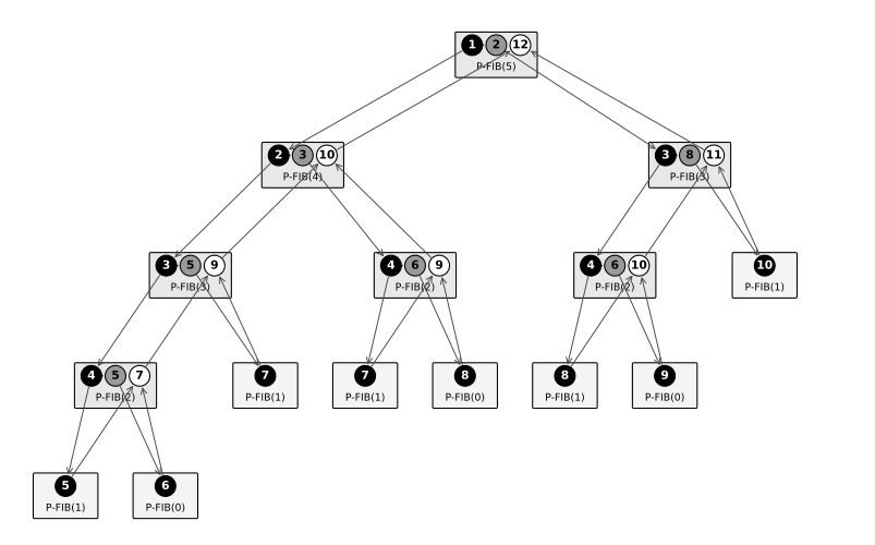
The number of strands run at each step is
| step | 1 | 2 | 3 | 4 | 5 | 6 | 7 | 8 | 9 | 10 | 11 | 12 |
|---|---|---|---|---|---|---|---|---|---|---|---|---|
| strands | 1 | 2 | 3 | 3 | 3 | 3 | 3 | 3 | 3 | 3 | 1 | 1 |
so \(T_3=12\), which is within the bound \(T_3\le 29/3+10\) of Theorem 27.1.
Show that a greedy scheduler satisfies a time bound slightly sharper than the one in Theorem 27.1:
\begin{equation*} T_P\le \frac{T_1-T_\infty}{P}+T_\infty . \qquad (27.5) \end{equation*}
Charge at least one unit of work to each incomplete step. With unit-time strands (as in the proof of Theorem 27.1), let \(c\) and \(k\) be the numbers of complete and incomplete steps, so \(T_P=c+k\).
The proof of Theorem 27.1 shows that every incomplete step lowers the span of the unexecuted dag by 1, so \(k\le T_\infty\). An incomplete step still runs at least one strand, because some strand is always ready while the computation is unfinished, so the incomplete steps do at least \(k\) units of work. The complete steps do exactly \(Pc\) units, hence \(Pc+k\le T_1\). Therefore
\begin{equation*} \begin{aligned} T_P=c+k&\le \frac{T_1-k}{P}+k =\frac{T_1}{P}+k\Bigl(1-\frac1P\Bigr)\\ &\le \frac{T_1}{P}+T_\infty\Bigl(1-\frac1P\Bigr) =\frac{T_1-T_\infty}{P}+T_\infty , \end{aligned} \end{equation*}
where the second inequality uses \(k\le T_\infty\) and \(1-1/P\ge 0\). \(\blacksquare\)
Build a computation dag on which two executions by greedy schedulers, on the same number of processors, can differ in running time by a factor close to 2. Describe how each execution proceeds.
Take a chain of \(k\) strands alongside \((P-1)k\) independent strands. On \(P\) processors one greedy execution takes \(k+2\) steps and another takes \(k(2-1/P)+2\), a ratio that tends to \(2-1/P\) as \(k\to\infty\). That ratio is as close to 2 as we like once \(P\) is large.
The dag, with unit-time strands, \(P\ge 2\), and \(k\) a multiple of \(P\), is as follows. An initial strand \(s\) has edges to \(u_1\) and to each of \(v_1,\dots,v_{(P-1)k}\). The chain runs \(u_1\to u_2\to\cdots\to u_k\). The final strand \(t\) has in-edges from \(u_k\) and from every \(v_i\). (Such a dag arises, for instance, from a parallel loop over \((P-1)k+1\) iterations, one of which is a serial loop of length \(k\).) So \(T_1=Pk+2\) and \(T_\infty=k+2\).
(i) Fast execution. Step 1 runs \(s\). At each of the next \(k\) steps the ready set holds one \(u_j\) plus at least \(P-1\) remaining \(v_i\)’s. The scheduler runs \(u_j\) and \(P-1\) of the \(v_i\)’s; this is a complete step, so it is greedy. After step \(k+1\) the chain and all \(v_i\)’s are finished, and step \(k+2\) runs \(t\):
\begin{equation*} T_P^{\mathrm{fast}}=k+2 . \end{equation*}
This is optimal by the span law (27.3).
(ii) Slow execution. Step 1 runs \(s\). While at least \(P\) of the \(v_i\)’s remain, the ready set has more than \(P\) strands, and the scheduler runs \(P\) of the \(v_i\)’s and leaves \(u_1\) waiting; these are complete steps, so this is greedy. Since \(P\mid (P-1)k\), the \(v_i\)’s are finished after \((P-1)k/P\) such steps. Then only one strand is ready at a time, and the incomplete steps run \(u_1,\dots,u_k\) and then \(t\):
\begin{equation*} T_P^{\mathrm{slow}}=1+\frac{(P-1)k}{P}+k+1=k\Bigl(2-\frac1P\Bigr)+2 . \end{equation*}
Hence
\begin{equation*} \frac{T_P^{\mathrm{slow}}}{T_P^{\mathrm{fast}}}\longrightarrow 2-\frac1P \quad (k\to\infty). \end{equation*}
For example, \(P=10\) and \(k=1000\) give \(1902/1002\approx 1.90\).
Professor Karan times her deterministic multithreaded algorithm with a greedy scheduler on an ideal parallel computer using 4, 10 and 64 processors. She reports \(T_4=80\) seconds, \(T_{10}=42\) seconds and \(T_{64}=10\) seconds. Show that the professor is either lying or incompetent. (Hint: combine the work law (27.2), the span law (27.3), and inequality (27.5) of Exercise 27.1-3.)
The three measurements imply \(T_{10}\le 41\), which contradicts the reported \(T_{10}=42\).
The algorithm is deterministic, so all three runs share the same work \(T_1\) and span \(T_\infty\). The span law (27.3) applied to the 64-processor run gives \(T_\infty\le T_{64}=10\). The work law (27.2) applied to the 4-processor run gives \(T_1\le 4T_4=320\). Since the scheduler is greedy, (27.5) holds with \(P=10\), and its right side \(T_1/P+T_\infty(1-1/P)\) is increasing in both \(T_1\) and \(T_\infty\):
\begin{equation*} T_{10}\le \frac{T_1}{10}+\frac{9}{10}T_\infty\le \frac{320}{10}+\frac{9}{10}\cdot 10=41<42 . \end{equation*}
So at least one of the three reported times is wrong.
Design a multithreaded algorithm that multiplies an \(n\times n\) matrix by an \(n\)-vector with \(\Theta(n^2)\) work and parallelism \(\Theta(n^2/\lg n)\).
Keep the parallel loop over rows in MAT-VEC, but compute each dot product \(y_i=\sum_{j=1}^n a_{ij}x_j\) by a divide-and-conquer parallel sum instead of a serial loop. The work stays \(\Theta(n^2)\) and the span drops to \(\Theta(\lg n)\).
MAT-VEC-FAST(A, x)
1 n = A.rows
2 let y be a new vector of length n
3 parallel for i = 1 to n
4 y[i] = ROW-SUM(A, x, i, 1, n)
5 return y
ROW-SUM(A, x, i, j, j')
1 if j == j'
2 return A[i][j] * x[j]
3 else mid = floor((j + j') / 2)
4 s = spawn ROW-SUM(A, x, i, j, mid)
5 t = ROW-SUM(A, x, i, mid + 1, j')
6 sync
7 return s + t
Correctness. By induction on \(j^{\prime}-j\), ROW-SUM\((A,x,i,j,j^{\prime})\) returns \(\sum_{l=j}^{j^{\prime}}a_{il}x_l\). The base case \(j=j^{\prime}\) is line 2. In the inductive step, \(s\) and \(t\) are the sums over \([j,\mathit{mid}]\) and \([\mathit{mid}+1,j^{\prime}]\) by the inductive hypothesis, and the sync ensures that both are available before line 7 adds them. The algorithm has no determinacy races: \(s\) and \(t\) are local to each instance, and iteration \(i\) of the parallel loop writes only \(y_i\). Hence \(y=Ax\).
Work and span. A call of ROW-SUM on \(m\) terms forms a full binary tree with \(m\) leaves and \(m-1\) internal nodes (Exercise B.5-3), each costing \(\Theta(1)\), so its work is \(\Theta(m)\). Its two halves run in parallel, so by Figure 27.3(b) its span satisfies \(S(m)=S(\lceil m/2\rceil)+\Theta(1)\), giving \(S(m)=\Theta(\lg m)\). The serialization of MAT-VEC-FAST does \(n\) row sums of \(n\) terms each, and the loop overhead is amortized as in the text, so
\begin{equation*} T_1(n)=n\cdot\Theta(n)=\Theta(n^2). \end{equation*}
The span of a parallel loop is \(\Theta(\lg n)\) plus the largest span of an iteration (Section 27.1), so
\begin{equation*} T_\infty(n)=\Theta(\lg n)+\max_{1\le i\le n}\Theta(\lg n)=\Theta(\lg n). \end{equation*}
The parallelism is therefore \(T_1/T_\infty=\Theta(n^2/\lg n)\).
The procedure P-TRANSPOSE\((A)\) transposes an \(n \times n\) matrix \(A\) in place: it sets \(n = A.rows\), then runs a parallel for loop over \(j = 2, \dots, n\), and inside it a parallel for loop over \(i = 1, \dots, j-1\) whose body exchanges \(a_{ij}\) with \(a_{ji}\). Determine the work, the span and the parallelism of this algorithm.
Work \(\Theta(n^2)\), span \(\Theta(\lg n)\), parallelism \(\Theta(n^2/\lg n)\).
The work is the running time of the serialization, which performs one constant-time exchange per pair \(i < j\), plus \(\Theta(n)\) outer-loop overhead:
\begin{equation*} T_1(n) = \Theta(n) + \sum_{j=2}^{n} \Theta(j-1) = \Theta\!\left(\frac{n(n-1)}{2}\right) = \Theta(n^2). \end{equation*}
For the span, use the parallel-loop formula of Section 27.1, \(T_\infty = \Theta(\lg(\text{iterations})) + \max_i \mathit{iter}_\infty(i)\). The inner loop for a fixed \(j\) has \(j-1\) iterations of span \(\Theta(1)\), so its span is \(\Theta(\lg j) + \Theta(1)\); the outer loop has \(n-1\) iterations, hence
\begin{equation*} T_\infty(n) = \Theta(\lg n) + \max_{2 \le j \le n} \bigl(\Theta(\lg j) + \Theta(1)\bigr) = \Theta(\lg n). \end{equation*}
Therefore the parallelism is
\begin{equation*} \frac{T_1(n)}{T_\infty(n)} = \Theta\!\left(\frac{n^2}{\lg n}\right). \end{equation*}
Modify P-TRANSPOSE from Exercise 27.1-7 by turning the parallel for loop of line 3 (the inner loop over \(i\)) into an ordinary serial for loop. Determine the work, the span and the parallelism of the modified algorithm.
Work \(\Theta(n^2)\), span \(\Theta(n)\), parallelism \(\Theta(n)\).
The serialization is unchanged, so as in Exercise 27.1-7 the work is \(T_1(n) = \sum_{j=2}^{n}\Theta(j-1) + \Theta(n) = \Theta(n^2)\). Iteration \(j\) of the outer parallel loop is now a serial loop of \(j-1\) constant-time exchanges, so its span is \(\Theta(j)\). By the parallel-loop span formula of Section 27.1, with \(n-1\) outer iterations,
\begin{equation*} T_\infty(n) = \Theta(\lg n) + \max_{2 \le j \le n} \Theta(j) = \Theta(\lg n) + \Theta(n) = \Theta(n), \end{equation*}
the maximum being attained at \(j = n\). Hence the parallelism is
\begin{equation*} \frac{T_1(n)}{T_\infty(n)} = \frac{\Theta(n^2)}{\Theta(n)} = \Theta(n). \end{equation*}
In the chess lesson of Section 27.1, the original program has work \(T_1 = 2048\) seconds and span \(T_\infty = 1\) second, while the optimized version has work \(T^{\prime}_1 = 1024\) seconds and span \(T^{\prime}_\infty = 8\) seconds. Taking the running time on \(P\) processors to be \(T_P = T_1/P + T_\infty\), find the number of processors at which the two versions run equally fast.
At \(P = 1024/7 \approx 146.3\) processors.
Equating the two approximations,
\begin{equation*} \frac{2048}{P} + 1 = \frac{1024}{P} + 8 \iff \frac{1024}{P} = 7 \iff P = \frac{1024}{7} \approx 146.29 . \end{equation*}
No integer \(P\) gives exactly equal times (\(T_P - T^{\prime}_P = 1024/P - 7\) is decreasing): for \(P \le 146\) the optimized version is faster (at \(P=146\): \(15.014 < 15.027\) seconds), and for \(P \ge 147\) the original is faster (at \(P=147\): \(14.932 < 14.966\) seconds).
27.2 Multithreaded matrix multiplication
Draw the computation dag of P-SQUARE-MATRIX-MULTIPLY run on \(2\times 2\) matrices, and say which part of the execution each vertex (strand) of your drawing stands for. Draw spawn and call edges pointing down, continuation edges pointing right, and return edges pointing up. Taking every strand to cost one unit of time, find the work, the span and the parallelism of this computation.
Work \(T_1 = 19\), span \(T_\infty = 11\), parallelism \(T_1/T_\infty = 19/11 \approx 1.73\).
Each parallel for loop is compiled into a divide-and-conquer helper exactly as MAT-VEC-MAIN-LOOP in Section 27.1, with the strand conventions of Figure 27.4: an internal helper instance with range \([i,i^{\prime}]\), \(i<i^{\prime}\), has three strands (up to the spawn of the first half; the call of the second half; after the sync), and an instance with \(i=i^{\prime}\) executes one iteration of the loop body. Here \(n=2\), so each helper has one internal instance and two leaves.
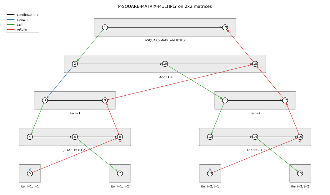
The vertices, numbered in the order of the serial execution:
| strand | part of the execution |
|---|---|
| 1 | lines 1-2, then the call of the loop of line 3 |
| 2, 10, 18 | I-LOOP(1,2): spawn iteration \(i=1\); call iteration \(i=2\); after the sync, return |
| 3, 11 | iteration \(i=1\), \(i=2\) of line 3: call the loop of line 4 |
| 9, 17 | iteration \(i=1\), \(i=2\) of line 3: return after that loop |
| 4, 6, 8 | J-LOOP(1,2) for \(i=1\): spawn \(j=1\); call \(j=2\); after the sync |
| 12, 14, 16 | J-LOOP(1,2) for \(i=2\): the same three strands |
| 5, 7, 13, 15 | lines 5-7 (the serial \(k\)-loop) for \((i,j)=(1,1),(1,2),(2,1),(2,2)\) |
| 19 | line 8, return \(C\) |
The work is the number of strands:
\begin{equation*} \begin{aligned} T_1 &= \underbrace{2}_{\text{main}} + \underbrace{3}_{\text{I-LOOP}} + \underbrace{2\cdot 2}_{i\text{-iterations}}\\ &\quad + \underbrace{2\cdot 3}_{\text{J-LOOPs}} + \underbrace{4}_{\text{bodies}} = 19 . \end{aligned} \end{equation*}
A path from strand 1 to strand 19 uses at most two strands of I-LOOP before descending, one strand of an \(i\)-iteration, at most two strands of a J-LOOP, one body strand, and then one strand each of the J-LOOP, the \(i\)-iteration, I-LOOP and the main procedure on the way back up, so it has at most \(1+2+1+2+1+1+1+1+1 = 11\) vertices. A path attaining this is
\begin{equation*} 1 \to 2 \to 10 \to 11 \to 12 \to 14 \to 15 \to 16 \to 17 \to 18 \to 19, \end{equation*}
so \(T_\infty = 11\) and the parallelism is \(19/11\).
Do Exercise 27.2-1 again, this time for P-MATRIX-MULTIPLY-RECURSIVE: draw its computation dag on \(2\times 2\) matrices (spawn and call edges down, continuation edges right, return edges up), say which part of the execution each strand is, and, with unit-time strands, find the work, span and parallelism.
Work \(T_1 = 35\), span \(T_\infty = 20\), parallelism \(35/20 = 1.75\).
The conventions are those of Exercise 27.2-1 (each parallel for is a divide-and-conquer helper as in Figure 27.4). With \(n=2\), the top-level call takes the recursive branch, and each of its eight recursive calls is on \(1\times 1\) matrices, so it is a single strand (lines 1-3). After the sync, lines 15-17 are the same doubly nested loop as in Exercise 27.2-1, with body \(c_{ij} = c_{ij}+t_{ij}\).
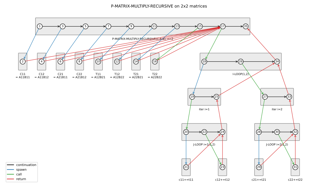
The vertices, numbered in the order of the serial execution:
| strand | part of the execution |
|---|---|
| 1 | lines 1-5, then the spawn in line 6 |
| 3, 5, 7, 9, 11, 13 | the spawns in lines 7-12, one each |
| 15 | the call in line 13 |
| 2, 4, …, 16 | the base cases \(C_{11}, C_{12}, C_{21}, C_{22}, T_{11}, T_{12}, T_{21}, T_{22}\) computed by lines 6-13 |
| 17 | after the sync of line 14, the call of the loop of line 15 |
| 18, 26, 34 | I-LOOP(1,2): spawn \(i=1\); call \(i=2\); after the sync |
| 19, 25 and 27, 33 | iterations \(i=1\) and \(i=2\) of line 15: call the loop of line 16; return |
| 20, 22, 24 and 28, 30, 32 | J-LOOP(1,2) for \(i=1\) and \(i=2\): spawn \(j=1\); call \(j=2\); after the sync |
| 21, 23, 29, 31 | line 17 for \((i,j)=(1,1),(1,2),(2,1),(2,2)\) |
| 35 | return from the procedure |
The work counts the strands:
\begin{equation*} \begin{aligned} T_1 &= \underbrace{10}_{\text{top level}} + \underbrace{8}_{\text{base cases}}\\ &\quad + \underbrace{3+2\cdot 2+2\cdot 3+4}_{\text{lines 15-17}} = 35 . \end{aligned} \end{equation*}
A path reaching strand 17 has at most nine earlier vertices (at most the eight top-level strands 1, 3, …, 15 and one base case), and the counting of Exercise 27.2-1 shows that a path through the loop from strand 18 to strand 34 has at most \(2+1+2+1+1+1+1 = 9\) vertices. Adding strand 35 gives \(T_\infty \le 10+9+1 = 20\), and this bound is reached by
\begin{equation*} \begin{aligned} &1\to3\to5\to7\to9\to11\to13\to15\to16\to17\\ &\quad\to18\to26\to27\to28\to30\to31\to32\to33\to34\to35 . \end{aligned} \end{equation*}
So \(T_\infty = 20\) and the parallelism is \(35/20 = 7/4\).
Write pseudocode for a multithreaded algorithm that multiplies two \(n\times n\) matrices using \(\Theta(n^3)\) work and only \(\Theta(\lg n)\) span, and analyze it.
Compute all \(n^3\) products \(a_{ik}b_{kj}\) at once into a temporary array, then form each \(c_{ij}\) by a divide-and-conquer parallel sum of its \(n\) products, so that the race in the inner loop of P-SQUARE-MATRIX-MULTIPLY disappears.
P-MATRIX-MULTIPLY-LG(A, B)
1 n = A.rows
2 let C be a new n x n matrix and D a new n x n x n array
3 parallel for i = 1 to n
4 parallel for j = 1 to n
5 parallel for k = 1 to n
6 d[i,j,k] = a[i,k] * b[k,j]
7 parallel for i = 1 to n
8 parallel for j = 1 to n
9 c[i,j] = P-SUM(D, i, j, 1, n)
10 return C
P-SUM(D, i, j, lo, hi)
1 if lo == hi
2 return d[i,j,lo]
3 mid = floor((lo + hi) / 2)
4 x = spawn P-SUM(D, i, j, lo, mid)
5 y = P-SUM(D, i, j, mid + 1, hi)
6 sync
7 return x + y
Correctness. By induction on \(hi-lo\), P-SUM returns \(\sum_{k=lo}^{hi} d_{ijk}\): the base case is line 2, and after the sync the two recursive results are the sums over \([lo,mid]\) and \([mid+1,hi]\). Hence line 9 sets \(c_{ij} = \sum_{k=1}^n a_{ik}b_{kj}\). There are no determinacy races: the iterations of lines 3-6 write distinct entries \(d_{ijk}\) and read only \(A\) and \(B\); the iterations of lines 7-9 write distinct entries \(c_{ij}\); and the two branches of P-SUM only read \(D\), each writing its own local variable.
Analysis. For P-SUM on \(m = hi-lo+1\) elements the recursion tree is a full binary tree with \(m\) leaves and \(m-1\) internal nodes (Exercise B.5-3), each doing \(\Theta(1)\) work, and its depth is \(\lceil \lg m\rceil\); so its work is \(\Theta(m)\) and its span is \(\Theta(1+\lg m)\). The work of the whole algorithm is that of its serialization (with loop overhead only a constant factor, Section 27.1), and the span of a parallel loop is \(\Theta(\lg n) + \max_i \mathit{iter}_\infty(i)\) (Section 27.1):
\begin{equation*} \begin{aligned} T_1(n) &= n^3\cdot\Theta(1) + n^2\cdot\Theta(n) = \Theta(n^3),\\ T_\infty(n) &= \underbrace{3\,\Theta(\lg n) + \Theta(1)}_{\text{lines 3-6}} + \underbrace{2\,\Theta(\lg n) + \Theta(\lg n)}_{\text{lines 7-9}}\\ &= \Theta(\lg n), \end{aligned} \end{equation*}
so the parallelism is \(\Theta(n^3/\lg n)\).
Write pseudocode for an efficient multithreaded algorithm that multiplies a \(p\times q\) matrix by a \(q\times r\) matrix, and analyze it. The algorithm must remain highly parallel even when one or more of \(p\), \(q\), \(r\) equals \(1\).
Generalize Exercise 27.2-3: form all \(pqr\) products in parallel, then reduce each of the \(pr\) length-\(q\) sums with P-SUM; this has work \(\Theta(pqr)\) and span \(\Theta(1+\lg(pqr))\).
P-RECT-MATRIX-MULTIPLY(A, B)
1 p = A.rows, q = A.columns, r = B.columns
2 let C be a new p x r matrix and D a new p x r x q array
3 parallel for i = 1 to p
4 parallel for j = 1 to r
5 parallel for k = 1 to q
6 d[i,j,k] = a[i,k] * b[k,j]
7 parallel for i = 1 to p
8 parallel for j = 1 to r
9 c[i,j] = P-SUM(D, i, j, 1, q)
10 return C
Here P-SUM is the procedure of Exercise 27.2-3, which returns \(\sum_{k=lo}^{hi} d_{ijk}\) with work \(\Theta(m)\) and span \(\Theta(1+\lg m)\) on \(m=hi-lo+1\) terms. Correctness and race-freedom are exactly as in Exercise 27.2-3: line 9 sets \(c_{ij} = \sum_{k=1}^q a_{ik}b_{kj}\), and distinct iterations write distinct locations while reading only \(A\), \(B\) or \(D\).
A parallel loop of \(m\) iterations has span \(\Theta(1+\lg m) + \max_i \mathit{iter}_\infty(i)\) by Section 27.1 (the \(1\) covers \(m=1\)). Therefore
\begin{equation*} \begin{aligned} T_1 &= pqr\cdot\Theta(1) + pr\cdot\Theta(q) = \Theta(pqr),\\ T_\infty &= \Theta(1+\lg p) + \Theta(1+\lg r) + \Theta(1+\lg q)\\ &= \Theta(1+\lg(pqr)), \end{aligned} \end{equation*}
and the parallelism is \(\Theta\bigl(pqr/(1+\lg(pqr))\bigr)\). The work equals the \(\Theta(pqr)\) running time of the serial triple loop, so the algorithm is work-efficient, and the parallelism stays nearly linear in the work whichever dimensions are \(1\): an inner product (\(p=r=1\)) gets \(\Theta(q/\lg q)\), a matrix-vector product (\(r=1\)) gets \(\Theta(pq/\lg(pq))\), and an outer product (\(q=1\)) gets \(\Theta(pr/\lg(pr))\).
Write pseudocode for an efficient multithreaded algorithm that transposes an \(n\times n\) matrix in place. It must use divide-and-conquer, recursively splitting the matrix into four \(n/2\times n/2\) submatrices, and it may not use parallel for loops. Analyze it.
Since \(\begin{pmatrix} A_{11} & A_{12}\\ A_{21} & A_{22}\end{pmatrix}^{T} = \begin{pmatrix} A_{11}^T & A_{21}^T\\ A_{12}^T & A_{22}^T\end{pmatrix}\), transpose \(A_{11}\) and \(A_{22}\) recursively in parallel with a recursive exchange of \(A_{12}\) and \(A_{21}^T\); this has work \(\Theta(n^2)\) and span \(\Theta(\lg n)\). Take \(n\) a power of \(2\) and call P-TRANSPOSE-DC\((A,1,n)\); P-SWAP-T\((A,r,c,s,t,n)\) exchanges \(a_{r+x,\,c+y}\) with \(a_{s+y,\,t+x}\) for all \(0\le x,y<n\).
P-TRANSPOSE-DC(A, i, n)
1 if n > 1
2 m = n / 2
3 spawn P-TRANSPOSE-DC(A, i, m)
4 spawn P-TRANSPOSE-DC(A, i + m, m)
5 P-SWAP-T(A, i, i + m, i + m, i, m)
6 sync
P-SWAP-T(A, r, c, s, t, n)
1 if n == 1
2 exchange a[r,c] with a[s,t]
3 else m = n / 2
4 spawn P-SWAP-T(A, r, c, s, t, m)
5 spawn P-SWAP-T(A, r, c + m, s + m, t, m)
6 spawn P-SWAP-T(A, r + m, c, s, t + m, m)
7 P-SWAP-T(A, r + m, c + m, s + m, t + m, m)
8 sync
Correctness. P-SWAP-T meets its specification by induction on \(n\) whenever the blocks \(X\) (corner \((r,c)\)) and \(Y\) (corner \((s,t)\)) are disjoint: writing \((x,y) = (x_0+\alpha m,\, y_0+\beta m)\) with \(\alpha,\beta\in\{0,1\}\), the pair \(a_{r+x,c+y} \leftrightarrow a_{s+y,t+x}\) is handled by exactly one of lines 4-7, namely the call with \(X\)-quadrant \((\alpha,\beta)\) and \(Y\)-quadrant \((\beta,\alpha)\). The four calls touch pairwise disjoint sets of entries, so they do not race. In P-TRANSPOSE-DC, line 5 exchanges \(A_{12}\) with \(A_{21}^T\) (corners \((i,i+m)\) and \((i+m,i)\), disjoint blocks), and by induction lines 3-4 replace \(A_{11}\), \(A_{22}\) by their transposes; the three branches touch the disjoint regions \(A_{11}\), \(A_{22}\) and \(A_{12}\cup A_{21}\), so there are no races and the result is the block form of \(A^T\) above.
Analysis. Let \(S_1, S_\infty\) and \(T_1, T_\infty\) be the work and span of P-SWAP-T and P-TRANSPOSE-DC. The four calls of P-SWAP-T run in parallel on size \(n/2\), as do the three branches of P-TRANSPOSE-DC:
\begin{equation*} \begin{aligned} S_1(n) &= 4S_1(n/2)+\Theta(1) = \Theta(n^2),\\ S_\infty(n) &= S_\infty(n/2)+\Theta(1) = \Theta(\lg n),\\ T_1(n) &= 2T_1(n/2)+S_1(n/2)+\Theta(1) = \Theta(n^2),\\ T_\infty(n) &= \max\{T_\infty(n/2),\, S_\infty(n/2)\}+\Theta(1). \end{aligned} \end{equation*}
The first two are cases 1 and 2 of the master theorem (\(n^{\log_2 4} = n^2\) dominates \(1\); \(n^{\log_2 1} = 1\) matches \(\Theta(1)\)). Then \(T_1(n) = 2T_1(n/2)+\Theta(n^2)\) is case 3 (\(n^2 = \Omega(n^{1+\epsilon})\), regularity \(2(n/2)^2 = \tfrac12 n^2\)). For \(T_\infty\), clearly \(T_\infty(n)\ge S_\infty(n/2) = \Omega(\lg n)\); conversely, if \(S_\infty(m)\le a\lg m+b\) and the \(\Theta(1)\) term is at most \(a\), then with \(B=\max\{b,T_\infty(1)\}\) induction gives
\begin{equation*} T_\infty(n) \le a\lg(n/2) + B + a = a\lg n + B . \end{equation*}
So \(T_\infty(n) = \Theta(\lg n)\) and the parallelism is \(\Theta(n^2/\lg n)\).
Write pseudocode for an efficient multithreaded implementation of the Floyd-Warshall algorithm of Section 25.2, which finds shortest-path weights between every pair of vertices of an edge-weighted directed graph, and analyze it.
Keep the outer \(k\)-loop of FLOYD-WARSHALL (page 695) serial and run the \(n^2\) updates of each round in a doubly nested parallel for, reading \(D^{(k-1)}\) and writing a second buffer for \(D^{(k)}\); this has work \(\Theta(n^3)\) and span \(\Theta(n\lg n)\).
P-FLOYD-WARSHALL(W)
1 n = W.rows
2 let D and E be new n x n matrices
3 parallel for i = 1 to n
4 parallel for j = 1 to n
5 d[i,j] = w[i,j]
6 for k = 1 to n
7 parallel for i = 1 to n
8 parallel for j = 1 to n
9 e[i,j] = min(d[i,j], d[i,k] + d[k,j])
10 exchange the names D and E
11 return D
Correctness. Loop invariant: at the start of each iteration of the loop of lines 6-10, \(D = D^{(k-1)}\). Initialization: lines 3-5 set \(D = W = D^{(0)}\). Maintenance: each iteration of lines 7-9 writes only its own entry \(e_{ij}\) and reads only \(D\), so there are no determinacy races and afterwards \(e_{ij} = \min\{d^{(k-1)}_{ij},\, d^{(k-1)}_{ik} + d^{(k-1)}_{kj}\} = d^{(k)}_{ij}\) by recurrence (25.5); line 10 (a \(\Theta(1)\) pointer exchange) makes \(D = D^{(k)}\). Termination: when \(k = n+1\), \(D = D^{(n)}\), which is the matrix of shortest-path weights by the analysis of Section 25.2.
Analysis. The serialization is FLOYD-WARSHALL with \(\Theta(n^2)\) extra initialization, so \(T_1(n) = \Theta(n^3)\). By the span formula for parallel loops in Section 27.1, lines 3-5 and each round of lines 7-9 have span \(\Theta(\lg n)+\Theta(\lg n)+\Theta(1) = \Theta(\lg n)\), and the \(n\) rounds run one after another:
\begin{equation*} T_\infty(n) = \Theta(\lg n) + n\bigl(\Theta(\lg n) + \Theta(1)\bigr) = \Theta(n\lg n), \end{equation*}
so the parallelism is \(\Theta(n^3/(n\lg n)) = \Theta(n^2/\lg n)\).
27.3 Multithreaded merge sort
Describe how the base case of the multithreaded merging procedure P-MERGE can be coarsened.
Stop recursing once the two subarrays together hold at most a constant grain size \(G\) of elements, and merge them with an ordinary serial merge loop directly into the output subarray \(A[p_3 \mathinner{.\,.} p_3+n_1+n_2-1]\). Everything else in P-MERGE stays the same. Since P-MERGE does not require the inputs to be adjacent, we cannot reuse MERGE’s sentinels, so the serial merge checks indices instead:
P-MERGE-COARSE(T, p1, r1, p2, r2, A, p3)
1 n1 = r1 - p1 + 1
2 n2 = r2 - p2 + 1
3 if n1 + n2 <= G // G = grain size, a constant
4 i = p1; j = p2
5 for k = p3 to p3 + n1 + n2 - 1
6 if j > r2 or (i <= r1 and T[i] <= T[j])
7 A[k] = T[i]; i = i + 1
8 else A[k] = T[j]; j = j + 1
9 return
10 if n1 < n2
11 exchange p1 with p2, r1 with r2, n1 with n2
12 q1 = floor((p1 + r1) / 2)
13 q2 = BINARY-SEARCH(T[q1], T, p2, r2)
14 q3 = p3 + (q1 - p1) + (q2 - p2)
15 A[q3] = T[q1]
16 spawn P-MERGE-COARSE(T, p1, q1 - 1, p2, q2 - 1, A, p3)
17 P-MERGE-COARSE(T, q1 + 1, r1, q2, r2, A, q3 + 1)
18 sync
Lines 4–8 are the usual serial merge: each step writes the smaller remaining front element, taking from the first subarray whenever the second is used up. So a call that hits the base case is correct. When \(n_1+n_2 > G \ge 0\) we have \(n_1 \ge 1\) after lines 10–11, so \(q_1\) is a valid index. Lines 10–18 are lines 3–6 and 8–15 of P-MERGE, and the book’s correctness argument carries over word for word.
The base case now costs \(\Theta(n_1+n_2) = O(G) = O(1)\) work and span. The rest of the analysis in Section 27.3 does not change. Recurrence (27.9) still gives \(\Theta(n)\) work, and recurrence (27.8), \(PM_\infty(n) = PM_\infty(3n/4) + \Theta(\lg n)\), still gives \(\Theta(\lg^2 n)\) span by Exercise 4.6-2. The parallelism stays \(\Theta(n/\lg^2 n)\), but the many tiny leaf calls, each paying a spawn and a binary search to place one element, become short serial loops.
P-MERGE splits the work around a median of the larger of the two subarrays. Consider a variant that instead splits around a median of all the elements of the two sorted subarrays together, found with the result of Exercise 9.3-8. Write pseudocode for an efficient multithreaded merging procedure based on this median-finding step, and analyze it.
Split at rank \(k = \lceil n/2 \rceil\) of the combined input, where \(n = n_1+n_2\). The binary search of Exercise 9.3-8, extended to unequal lengths and an arbitrary rank \(k\), finds in serial time \(O(\lg n)\) a count \(i\) such that the \(k\) smallest elements are exactly \(T[p_1 \mathinner{.\,.} p_1+i-1]\) together with \(T[p_2 \mathinner{.\,.} p_2+k-i-1]\). We then merge the low halves into \(A[p_3 \mathinner{.\,.} p_3+k-1]\) and the high halves into \(A[p_3+k \mathinner{.\,.} p_3+n-1]\) in parallel. The resulting bounds are \(\Theta(n)\) work, \(\Theta(\lg^2 n)\) span and \(\Theta(n/\lg^2 n)\) parallelism.
TWO-SPLIT(T, p1, n1, p2, n2, k)
1 lo = max(0, k - n2); hi = min(k, n1)
2 while lo < hi
3 mid = floor((lo + hi) / 2)
4 if T[p1 + mid] < T[p2 + k - mid - 1]
5 lo = mid + 1
6 else hi = mid
7 return lo
P-MERGE-MED(T, p1, r1, p2, r2, A, p3)
1 n1 = r1 - p1 + 1; n2 = r2 - p2 + 1; n = n1 + n2
2 if n == 0 return
3 if n == 1
4 if n1 == 1 then A[p3] = T[p1] else A[p3] = T[p2]
5 return
6 k = ceil(n / 2); i = TWO-SPLIT(T, p1, n1, p2, n2, k)
7 spawn P-MERGE-MED(T, p1, p1 + i - 1, p2, p2 + k - i - 1, A, p3)
8 P-MERGE-MED(T, p1 + i, r1, p2 + k - i, r2, A, p3 + k)
9 sync
Split correctness: let \(P(i)\) be the predicate “\(i < \min(k,n_1)\) and \(T[p_1+i] < T[p_2+k-i-1]\)”. Inside the loop \(\mathit{mid} < \mathit{hi} \le \min(k,n_1)\) and \(1 \le k-\mathit{mid} \le n_2\), so both indices in line 4 are valid. \(P\) is monotone, because for \(i^{\prime} < i\),
\begin{equation*} T[p_1+i^{\prime}] \le T[p_1+i] < T[p_2+k-i-1] \le T[p_2+k-i^{\prime}-1] . \end{equation*}
Hence TWO-SPLIT returns the least \(i\) in \([\max(0,k-n_2), \min(k,n_1)]\) with \(P(i)\) false. For that \(i\):
- (i) if \(i \ge 1\) and \(k-i < n_2\), then \(P(i-1)\) holds, so \(T[p_1+i-1] < T[p_2+k-i]\);
- (ii) if \(i < n_1\) and \(k-i \ge 1\), then \(i < \min(k,n_1)\) and \(P(i)\) fails, so \(T[p_2+k-i-1] \le T[p_1+i]\).
Both input subarrays are sorted, so (i) and (ii) say that every chosen element is at most every unchosen one. The chosen elements are therefore \(k\) smallest elements overall.
Merge correctness, by strong induction on \(n\). The cases \(n \le 1\) are immediate. For \(n \ge 2\) we have \(1 \le k \le n-1\), so both recursive calls are strictly smaller. By induction they write the sorted low part into \(A[p_3 \mathinner{.\,.} p_3+k-1]\) and the sorted high part after it. Every low element is at most every high element, so the concatenation is sorted. The two calls read only \(T\) and write disjoint parts of \(A\), so they cannot race.
Analysis: each recursive call gets at most \(\lceil n/2 \rceil\) elements, and lines 1–6 cost \(O(\lg n)\). That cost is \(\Theta(\lg n)\) when the inputs interleave perfectly, because then every level of the recursion has \(n_1 \approx n_2\). In the worst case this gives
\begin{equation*} \begin{aligned} MM_\infty(n) &= MM_\infty(\lceil n/2 \rceil) + \Theta(\lg n) = \Theta(\lg^2 n), \\ MM_1(n) &= MM_1(\lceil n/2 \rceil) + MM_1(\lfloor n/2 \rfloor) + \Theta(\lg n) = \Theta(n). \end{aligned} \end{equation*}
The span recurrence is solved by Exercise 4.6-2, with \(a=1\), \(b=2\) and \(f(n) = \Theta(n^{\log_2 1}\lg n)\). The work recurrence is case 1 of the master theorem, since \(\lg n = O(n^{1-\epsilon})\). The parallelism is \(\Theta(n/\lg^2 n)\).
Design an efficient multithreaded algorithm that partitions an array around a pivot, in the way the PARTITION procedure of Section 7.1 (page 171) does: it uses the last element \(x = A[r]\) as the pivot and returns an index \(q\) with every element of the low side \(\le x\), the pivot at position \(q\), and every element of the high side \(> x\). The partition need not be done in place. Make the algorithm as parallel as possible and analyze it. (Hint: an auxiliary array and more than one pass over the input may be needed.)
Flag each element as low (\(\le x\)) or high (\(> x\)), and compute prefix sums of the flags with P-SCAN-3 from Problem 27-4, which takes \(\Theta(n)\) work and \(\Theta(\lg n)\) span. Then scatter every element in parallel to the slot its prefix sum gives it in an output array \(B\). The algorithm has \(\Theta(n)\) work, \(\Theta(\lg n)\) span and \(\Theta(n/\lg n)\) parallelism.
P-PARTITION(A, p, r, B) // partitions A[p..r] into B[p..r]
1 n = r - p + 1; x = A[r]
2 if n == 1
3 B[p] = x; return p
4 let lo[1..n-1] and hi[1..n-1] be new arrays
5 parallel for i = 1 to n - 1
6 if A[p + i - 1] <= x
7 lo[i] = 1; hi[i] = 0
8 else lo[i] = 0; hi[i] = 1
9 L = spawn P-SCAN-3(lo) // L[i] = lo[1] + ... + lo[i]
10 H = P-SCAN-3(hi) // H[i] = hi[1] + ... + hi[i]
11 sync
12 q = p + L[n - 1]; B[q] = x
13 parallel for i = 1 to n - 1
14 if lo[i] == 1
15 B[p + L[i] - 1] = A[p + i - 1]
16 else B[q + H[i]] = A[p + i - 1]
17 return q
Correctness: \(L[n-1]\) counts the low elements of \(A[p \mathinner{.\,.} r-1]\), and \(H[n-1] = (n-1) - L[n-1] = r-q\) counts the high ones. The \(j\)th low element in left-to-right order has \(L[i] = j\), so line 15 maps the low elements one-to-one onto \(B[p \mathinner{.\,.} q-1]\). Likewise line 16 maps the high elements one-to-one onto \(B[q+1 \mathinner{.\,.} r]\), and line 12 puts \(x\) at \(B[q]\). Thus \(B[p \mathinner{.\,.} r]\) is a permutation of \(A[p \mathinner{.\,.} r]\) with
\begin{equation*} B[p \mathinner{.\,.} q-1] \le x = B[q] < B[q+1 \mathinner{.\,.} r] , \end{equation*}
which is exactly PARTITION’s postcondition. The iterations of each parallel loop write distinct locations, and the two scans write different arrays, so there are no determinacy races.
Analysis: by Section 27.1, a parallel for loop over \(n-1\) constant-time iterations has \(\Theta(n)\) work and \(\Theta(\lg n)\) span. Each P-SCAN-3 has \(\Theta(n)\) work and \(\Theta(\lg n)\) span by Problem 27-4(e). The remaining lines are \(\Theta(1)\). In total,
\begin{equation*} T_1(n) = \Theta(n), \qquad T_\infty(n) = \Theta(\lg n), \qquad T_1/T_\infty = \Theta(n/\lg n). \end{equation*}
Write a multithreaded version of the RECURSIVE-FFT procedure of Section 30.2 (page 911), which computes the DFT of a coefficient vector \(a = (a_0, \ldots, a_{n-1})\) with \(n\) a power of 2. Make it as parallel as possible and analyze it.
Spawn the two half-size recursive transforms. Do the even/odd split and the butterfly loop of lines 10–13 as parallel for loops. In the butterfly loop, iteration \(k\) computes its own twiddle factor \(\omega_n^k\) instead of reading the running product \(\omega\), which would chain the iterations together. The result has \(\Theta(n\lg n)\) work, \(\Theta(\lg^2 n)\) span and \(\Theta(n/\lg n)\) parallelism.
P-RECURSIVE-FFT(a)
1 n = a.length // n is a power of 2
2 if n == 1
3 return a
4 let a0[0..n/2-1], a1[0..n/2-1], y[0..n-1] be new arrays
5 parallel for k = 0 to n/2 - 1
6 a0[k] = a[2k]
7 a1[k] = a[2k+1]
8 y0 = spawn P-RECURSIVE-FFT(a0)
9 y1 = P-RECURSIVE-FFT(a1)
10 sync
11 parallel for k = 0 to n/2 - 1
12 w = e^(2 pi i k / n) // w = omega_n^k
13 y[k] = y0[k] + w * y1[k]
14 y[k + n/2] = y0[k] - w * y1[k]
15 return y
Correctness: in RECURSIVE-FFT, lines 4, 5 and 13 make \(\omega = \omega_n^k\) in iteration \(k\). Line 12 here computes the same value directly, at \(O(1)\) cost, the same cost model that line 4 of RECURSIVE-FFT already uses. So every \(y_k\) and \(y_{k+n/2}\) gets the value that RECURSIVE-FFT assigns, and the result is \(\mathrm{DFT}_n(a)\). The two spawned calls work on separate arrays. Within each parallel loop, iteration \(k\) writes only entries indexed by \(k\) and reads only the inputs, so there are no determinacy races.
Analysis: the two parallel loops cost \(\Theta(n)\) work and \(\Theta(\lg n)\) span (Section 27.1), and the two recursive calls run in parallel. Hence
\begin{equation*} \begin{aligned} T_1(n) &= 2T_1(n/2) + \Theta(n) = \Theta(n \lg n), \\ T_\infty(n) &= T_\infty(n/2) + \Theta(\lg n) = \Theta(\lg^2 n). \end{aligned} \end{equation*}
The work recurrence is case 2 of the master theorem. The span recurrence follows from Exercise 4.6-2 with \(a=1\), \(b=2\) and \(f(n)=\Theta(n^{0}\lg n)\). The parallelism is \(T_1/T_\infty = \Theta(n\lg n/\lg^2 n) = \Theta(n/\lg n)\).
Write a multithreaded version of RANDOMIZED-SELECT (Section 9.2, page 216), which returns the \(i\)th smallest element of \(A[p \mathinner{.\,.} r]\). Make it as parallel as possible and analyze it. (Hint: use the partitioning algorithm of Exercise 27.3-3.)
Keep RANDOMIZED-SELECT’s structure but replace RANDOMIZED-PARTITION by a random pivot swap followed by P-PARTITION from Exercise 27.3-3. That partition is not in place, so the input array and a scratch array of the same index range swap roles at each level. For distinct elements, as assumed in Section 9.2, the expected work is \(\Theta(n)\) and the expected span is \(O(\lg^2 n)\).
P-RANDOMIZED-SELECT(A, p, r, i, B) // B: scratch, same index range as A
1 if p == r
2 return A[p]
3 j = RANDOM(p, r)
4 exchange A[j] with A[r]
5 q = P-PARTITION(A, p, r, B)
6 k = q - p + 1
7 if i == k
8 return B[q]
9 elseif i < k
10 return P-RANDOMIZED-SELECT(B, p, q - 1, i, A)
11 else return P-RANDOMIZED-SELECT(B, q + 1, r, i - k, A)
Correctness: by Exercise 27.3-3, \(B[p \mathinner{.\,.} r]\) is a permutation of \(A[p \mathinner{.\,.} r]\) with \(B[p \mathinner{.\,.} q-1] < B[q] < B[q+1 \mathinner{.\,.} r]\), where the pivot \(B[q]\) was chosen uniformly at random. That is the state RANDOMIZED-SELECT has after line 3, except that the data now sits in \(B\). The rest of the argument in Section 9.2 applies unchanged. \(A\) is free to serve as scratch for the recursive call, which touches only the subarray it is given.
Analysis: a call on \(m\) elements costs at most \(cm\) work and at most \(c\lg m + c\) span, by Exercise 27.3-3. Let the pivot’s rank be \(s\), uniform on \(\{1, \ldots, m\}\). The recursive call, if there is one, gets at most \(\max(s-1, m-s)\) elements, and this is \(\le 3m/4\) whenever \(m/4 \le s \le 3m/4+1\). At least \(m/2\) of the \(m\) ranks satisfy this, so
\begin{equation*} \Pr\{\text{next size} \le 3m/4\} \ge 1/2 . \end{equation*}
Say a call belongs to phase \(j\) if its size \(m\) satisfies \((3/4)^{j+1}n < m \le (3/4)^j n\). There are at most \(\log_{4/3} n + 1\) phases. Every call in phase \(j\) ends the phase with probability at least \(1/2\), whatever happened before. So the number of calls in phase \(j\) is dominated by a geometric random variable with success probability \(1/2\), and its expectation is at most 2. Summing over phases,
\begin{equation*} \begin{aligned} \mathrm{E}[T_1(n)] &\le \sum_{j \ge 0} 2c\,(3/4)^j n = 8cn , \\ \mathrm{E}[T_\infty(n)] &\le 2(\log_{4/3} n + 1)(c\lg n + c) = O(\lg^2 n) . \end{aligned} \end{equation*}
The first partition already costs \(\Omega(n)\) work, so \(\mathrm{E}[T_1(n)] = \Theta(n)\). The ratio \(\mathrm{E}[T_1]/\mathrm{E}[T_\infty]\) is therefore \(\Omega(n/\lg^2 n)\).
Show how to multithread the worst-case linear-time selection algorithm SELECT of Section 9.3, which finds the \(i\)th smallest of \(n\) distinct elements. Make the implementation as parallel as possible and analyze it.
Run each of SELECT’s non-recursive steps in parallel with \(\Theta(\lg n)\) span:
- the \(\lceil n/5 \rceil\) group medians are computed by a parallel for loop;
- the median-of-medians \(x\) is moved to the end of the array by a parallel search;
- the partition is done with P-PARTITION from Exercise 27.3-3.
The two recursive calls stay sequential, because the second one depends on \(x\). The work is \(\Theta(n)\) and the span is \(O(n^{p})\), where \(p \approx 0.8398\) is the root of \((1/5)^p + (7/10)^p = 1\).
P-SELECT(A, p, r, i) // ith smallest of distinct A[p..r]
1 n = r - p + 1
2 if n < 140
3 sort A[p..r] serially; return A[p + i - 1]
4 m = ceil(n / 5)
5 let M[1..m] and B[p..r] be new arrays
6 parallel for g = 1 to m // insertion-sort a group of <= 5
7 M[g] = lower median of A[p + 5(g-1) .. min(p + 5g - 1, r)]
8 x = P-SELECT(M, 1, m, floor((m + 1) / 2))
9 parallel for j = p to r
10 if A[j] == x
11 s = j // exactly one iteration writes s
12 exchange A[s] with A[r]
13 q = P-PARTITION(A, p, r, B)
14 k = q - p + 1
15 if i == k
16 return x
17 elseif i < k
18 return P-SELECT(B, p, q - 1, i)
19 else return P-SELECT(B, q + 1, r, i - k)
Correctness: lines 4–8 compute the median-of-medians \(x\) of steps 1–3 of SELECT. The elements are distinct, so exactly one \(j\) has \(A[j] = x\), line 11 has no race, and line 12 makes \(x\) the pivot that P-PARTITION uses. Lines 13–19 are steps 4–5 of SELECT, by Exercise 27.3-3. Each parallel loop iteration reads \(A\) and writes only its own location (\(M[g]\) or \(s\)).
Analysis: Section 9.3 shows that the recursive call in line 18 or 19 gets at most \(7n/10+6\) elements. Lines 6–7, 9–11 and 13 each cost \(\Theta(n)\) work and \(\Theta(\lg n)\) span, by Section 27.1 and Exercise 27.3-3. Lines 8 and 18–19 run one after the other. Assuming monotonicity, as Section 9.3 does, for \(n \ge 140\),
\begin{equation*} \begin{aligned} T_1(n) &\le T_1(\lceil n/5 \rceil) + T_1(7n/10+6) + \Theta(n) , \\ T_\infty(n) &\le T_\infty(\lceil n/5 \rceil) + T_\infty(7n/10+6) + \Theta(\lg n) . \end{aligned} \end{equation*}
The first recurrence is exactly the one solved in Section 9.3, so \(T_1(n) = O(n)\). The work is also \(\Omega(n)\), since every element is read, so \(T_1(n) = \Theta(n)\).
For the span we use the Akra–Bazzi method, recurrence (4.30) in the Chapter 4 notes. In Leighton’s form it tolerates the ceiling and the \(+6\), and it applies with \(a_1 = a_2 = 1\), \(b_1 = 1/5\), \(b_2 = 7/10\) and \(f(u) = \lg u\). The exponent \(p\) solves \((1/5)^p + (7/10)^p = 1\), so \(p = 0.8398\ldots\), and the integral term is bounded:
\begin{equation*} 0 \le \int_1^n \frac{\lg u}{u^{p+1}}\,du \le \int_1^\infty \frac{\lg u}{u^{p+1}}\,du = \frac{1}{p^2 \ln 2} . \end{equation*}
Hence \(T_\infty(n) = O(n^{p}) = O(n^{0.84})\), and the parallelism is \(\Omega(n^{1-p}) = \Omega(n^{0.16})\).
Method (2): use groups of a larger odd constant size \(g\). Each group median then costs \(O(g^2) = O(1)\) serially. The counting argument of Section 9.3 shows that at least \(\frac{g+1}{2}\bigl(\frac{1}{2}\lceil n/g \rceil - 2\bigr)\) elements lie on each side of \(x\), so the recursive call gets at most \((\frac34 - \frac{1}{4g})n + g + 1\) elements. Since \(\frac1g + \frac34 - \frac{1}{4g} < 1\), the Akra–Bazzi exponent for the work is below 1, and the work stays \(\Theta(n)\). The span is \(O(n^{p_g})\), where \(p_g\) solves \(g^{-p} + (\frac34 - \frac{1}{4g})^p = 1\). For example, \(p_{25} \approx 0.573\). As \(g \to \infty\), \(p_g \to 0\), because for any fixed \(\epsilon > 0\) we have \(g^{-\epsilon} + (3/4)^{\epsilon} < 1\) once \(g\) is large. So for every \(\epsilon > 0\) some constant \(g\) gives span \(O(n^{\epsilon})\) with linear work.
Problems for Chapter 27
Implementing parallel loops using nested parallelism: The procedure SUM-ARRAYS\((A,B,C)\) adds two \(n\)-element arrays \(A[1..n]\) and \(B[1..n]\) pairwise into \(C[1..n]\) with a single loop: parallel for \(i = 1\) to \(A.length\), set \(C[i] = A[i] + B[i]\).
(a) Rewrite this parallel loop with nested parallelism (spawn and sync), in the style of MAT-VEC-MAIN-LOOP, and analyze the parallelism of your implementation.
An alternative implementation SUM-ARRAYS’\((A,B,C)\) uses a parameter grain-size, still to be chosen: it sets \(n = A.length\), \(r = \lceil n/\text{grain-size} \rceil\), and then in an ordinary (serial) for loop over \(k = 0, 1, \ldots, r-1\) it spawns ADD-SUBARRAY\((A,B,C,\,k \cdot \text{grain-size} + 1,\,\min((k+1)\cdot\text{grain-size}, n))\); after the loop it syncs. ADD-SUBARRAY\((A,B,C,i,j)\) serially sets \(C[k] = A[k] + B[k]\) for \(k = i, \ldots, j\).
(b) If grain-size \(= 1\), what is the parallelism of this implementation?
(c) Give a formula for the span of SUM-ARRAYS’ in terms of \(n\) and grain-size, and derive the value of grain-size that maximizes parallelism.
(a) Divide and conquer on the index range exactly as MAT-VEC-MAIN-LOOP does; the work is \(\Theta(n)\), the span \(\Theta(\lg n)\), so the parallelism is \(\Theta(n/\lg n)\).
SUM-ARRAYS(A, B, C)
1 ADD-LOOP(A, B, C, 1, A.length)
ADD-LOOP(A, B, C, i, j)
1 if i == j
2 C[i] = A[i] + B[i]
3 else mid = floor((i + j) / 2)
4 spawn ADD-LOOP(A, B, C, i, mid)
5 ADD-LOOP(A, B, C, mid + 1, j)
6 sync
The two recursive calls touch disjoint index ranges, so there is no determinacy race, and by induction on \(j - i\) every \(C[k]\), \(i \le k \le j\), is set. The recursion tree is a full binary tree with \(n\) leaves and \(n-1\) internal nodes, each costing \(\Theta(1)\), and its height is \(\lceil \lg n \rceil\), so
\begin{equation*} \begin{aligned} T_1(n) &= T_1(\lceil n/2 \rceil) + T_1(\lfloor n/2 \rfloor) + \Theta(1) = \Theta(n), \\ T_\infty(n) &= T_\infty(\lceil n/2 \rceil) + \Theta(1) = \Theta(\lg n), \\ T_1(n)/T_\infty(n) &= \Theta(n/\lg n). \end{aligned} \end{equation*}
(b) The parallelism is \(\Theta(1)\). With grain-size \(=1\) we have \(r = n\) and each spawned ADD-SUBARRAY does one addition, so the work is \(\Theta(n)\). But the \(n\) spawns are issued one after another by the serial for loop of the parent strand, so the path through all \(n\) loop iterations to the last spawned child and then the sync has length \(\Theta(n)\); the span is \(\Theta(n)\) and \(T_1/T_\infty = \Theta(1)\).
(c) Writing \(g\) for grain-size (\(1 \le g \le n\)), the span is \(\Theta(n/g + g)\), and \(g = \sqrt n\) is optimal, which gives span \(\Theta(\sqrt n)\) and parallelism \(\Theta(\sqrt n)\). The \(k\)th child (for \(k = 0, \ldots, r-1\)) is spawned after \(k+1\) loop iterations of \(\Theta(1)\) each and then runs serially over \(L_k \le g\) elements, with \(L_0 = \min(g,n) = g\). So
\begin{equation*} \begin{aligned} T_\infty &= \Theta\bigl(\max_{0 \le k < r} (k + 1 + L_k)\bigr), \\ \max(r, g) \le \max_k (k+1+L_k) &\le r + g, \end{aligned} \end{equation*}
(the lower bound comes from the cases \(k = r-1\) and \(k = 0\)). Hence \(T_\infty = \Theta(r + g) = \Theta(\lceil n/g \rceil + g)\). The work is \(\Theta(r + n) = \Theta(n)\) whatever \(g\) is, so maximizing parallelism means minimizing \(n/g + g\). By the AM-GM inequality,
\begin{equation*} \frac{n}{g} + g \ge 2\sqrt{n}, \quad \text{with equality iff } g = \sqrt n . \end{equation*}
So grain-size \(= \sqrt n\) (rounded to an integer) is optimal. It gives \(T_\infty = \Theta(\sqrt n)\) and parallelism \(\Theta(n)/\Theta(\sqrt n) = \Theta(\sqrt n)\).
Saving temporary space in matrix multiplication: P-MATRIX-MULTIPLY-RECURSIVE has to allocate a temporary \(n \times n\) matrix \(T\), which can hurt the constants hidden in the \(\Theta\)-notation. Its parallelism is high, though. Ignoring constants, for \(1000 \times 1000\) matrices it is about \(1000^3/10^2 = 10^7\) (since \(\lg 1000 \approx 10\)), which is far more processors than most parallel machines have.
(a) Describe a recursive multithreaded algorithm that needs no temporary matrix \(T\), at the price of a span of \(\Theta(n)\). (Hint: compute \(C = C + AB\) with the general strategy of P-MATRIX-MULTIPLY-RECURSIVE, but initialize \(C\) in parallel and put a sync in a well-chosen place.)
(b) Give and solve recurrences for the work and the span of your implementation.
(c) Analyze the parallelism of your implementation. Ignoring the constants in the \(\Theta\)-notation, estimate it for \(1000 \times 1000\) matrices and compare it with the parallelism of P-MATRIX-MULTIPLY-RECURSIVE.
(a) Zero \(C\) with a doubly nested parallel loop, then accumulate \(C = C + AB\) recursively. In each call, the four products \(A_{i1}B_{1j}\) are added into the four quadrants \(C_{ij}\) in parallel, then a sync, then the four products \(A_{i2}B_{2j}\) are added in parallel. As in Section 27.2, \(n\) is an exact power of 2, the partition follows equation (27.6), and it takes \(\Theta(1)\) by index calculation.
P-MATRIX-MULTIPLY-NO-TEMP(C, A, B)
1 n = A.rows
2 parallel for i = 1 to n
3 parallel for j = 1 to n
4 c_ij = 0
5 P-MATRIX-MULTIPLY-ADD(C, A, B, n)
P-MATRIX-MULTIPLY-ADD(C, A, B, n) // C = C + A B
1 if n == 1
2 c_11 = c_11 + a_11 b_11
3 else partition A, B, C into n/2 x n/2 submatrices
4 spawn P-MATRIX-MULTIPLY-ADD(C_11, A_11, B_11, n/2)
5 spawn P-MATRIX-MULTIPLY-ADD(C_12, A_11, B_12, n/2)
6 spawn P-MATRIX-MULTIPLY-ADD(C_21, A_21, B_11, n/2)
7 P-MATRIX-MULTIPLY-ADD(C_22, A_21, B_12, n/2)
8 sync
9 spawn P-MATRIX-MULTIPLY-ADD(C_11, A_12, B_21, n/2)
10 spawn P-MATRIX-MULTIPLY-ADD(C_12, A_12, B_22, n/2)
11 spawn P-MATRIX-MULTIPLY-ADD(C_21, A_22, B_21, n/2)
12 P-MATRIX-MULTIPLY-ADD(C_22, A_22, B_22, n/2)
13 sync
Correctness: we show by induction on \(n\) that P-MATRIX-MULTIPLY-ADD replaces \(C\) by \(C + AB\) and has no determinacy race. The case \(n = 1\) is line 2. For \(n > 1\), the four calls in lines 4–7 write four disjoint quadrants of \(C\) and only read \(A\) and \(B\), so they are race-free; the same holds for lines 9–12. The sync in line 8 orders every update to a quadrant \(C_{ij}\) in the first phase before the second-phase update to that quadrant. By the inductive hypothesis, each quadrant therefore ends up as
\begin{equation*} C_{ij} + A_{i1}B_{1j} + A_{i2}B_{2j} = (C + AB)_{ij} \end{equation*}
by equation (27.6). Since lines 2–4 of the driver set \(C = 0\), the driver leaves \(C = AB\). No storage beyond \(C\) is allocated.
(b) The work is \(\Theta(n^3)\) and the span is \(\Theta(n)\). Let \(M_1(n)\) and \(M_\infty(n)\) be the work and span of P-MATRIX-MULTIPLY-ADD. There are eight half-size calls plus \(\Theta(1)\) for partitioning and spawning. The two phases run one after the other because of the sync in line 8, and within a phase the span is that of one call, so
\begin{equation*} \begin{aligned} M_1(n) &= 8M_1(n/2) + \Theta(1) = \Theta(n^3), \\ M_\infty(n) &= 2M_\infty(n/2) + \Theta(1) = \Theta(n). \end{aligned} \end{equation*}
Both recurrences fall under case 1 of the master theorem (Theorem 4.1). For the work, \(n^{\log_2 8} = n^3\) and \(\Theta(1) = O(n^{3-\epsilon})\). For the span, \(n^{\log_2 2} = n\) and \(\Theta(1) = O(n^{1-\epsilon})\). The doubly nested parallel loop that zeroes \(C\) has work \(\Theta(n^2)\) and span \(\Theta(\lg n)\) (Section 27.1), so the whole algorithm has work \(\Theta(n^3) + \Theta(n^2) = \Theta(n^3)\) and span \(\Theta(n) + \Theta(\lg n) = \Theta(n)\).
(c) The parallelism is \(\Theta(n^3)/\Theta(n) = \Theta(n^2)\). Ignoring constants, for \(n = 1000\) it is \(1000^2 = 10^6\). P-MATRIX-MULTIPLY-RECURSIVE, whose parallelism is \(\Theta(n^3/\lg^2 n)\), gets about \(10^7\), so the new algorithm has about one tenth of that parallelism (a factor of \(\lg^2 n / n \approx 1/10\)), which still far exceeds the processor count of almost any machine.
Multithreaded matrix algorithms:
(a) Give multithreaded pseudocode parallelizing the procedure LU-DECOMPOSITION of Section 28.1 (page 821). Make it as parallel as you can, and analyze its work, span and parallelism.
(b) Do the same for LUP-DECOMPOSITION (page 824).
(c) Do the same for LUP-SOLVE (page 817).
(d) Do the same for a multithreaded algorithm that inverts a symmetric positive-definite matrix using equation (28.13), i.e. for \(A = \begin{pmatrix} B & C^{\mathrm T} \\ C & D \end{pmatrix}\) with Schur complement \(S = D - CB^{-1}C^{\mathrm T}\),
\begin{equation*} A^{-1} = \begin{pmatrix} B^{-1} + B^{-1}C^{\mathrm T}S^{-1}CB^{-1} & -B^{-1}C^{\mathrm T}S^{-1} \\ -S^{-1}CB^{-1} & S^{-1} \end{pmatrix}. \end{equation*}
(a) Keep the outer loop over pivots serial and turn every inner loop into a parallel for: work \(\Theta(n^3)\), span \(\Theta(n\lg n)\), parallelism \(\Theta(n^2/\lg n)\).
P-LU-DECOMPOSITION(A)
1 n = A.rows
2 let L and U be new n x n matrices
3 parallel for i = 1 to n
4 parallel for j = 1 to n
5 u_ij = 0
6 if i == j then l_ij = 1 else l_ij = 0
7 for k = 1 to n
8 u_kk = a_kk
9 parallel for i = k + 1 to n
10 l_ik = a_ik / a_kk
11 u_ki = a_ki
12 parallel for i = k + 1 to n
13 parallel for j = k + 1 to n
14 a_ij = a_ij - l_ik * u_kj
15 return L and U
Every parallel loop is free of determinacy races: iterations of lines 9-11 write distinct entries \(l_{ik}, u_{ki}\) and read only \(A\); iterations of lines 12-14 write distinct entries \(a_{ij}\) with \(i,j>k\) and read only \(l_{ik}\) and \(u_{kj}\), which no iteration writes. Hence each loop computes exactly what the serial loop of LU-DECOMPOSITION computes, and correctness is that of Section 28.1 (zeroing all of \(U\) in line 5 is harmless, since every entry with \(i\le j\) is overwritten in line 8 or 11). The step-\(k\) iteration cannot start before step \(k-1\) is finished, because its pivot \(a_{kk}\) is an entry of the Schur complement produced by step \(k-1\).
The parallel-for control adds only work linear in the number of iterations (Section 27.1), so the work is that of the serial code, \(T_1(n)=\Theta(n^3)\). A parallel for with \(m\) iterations of \(\Theta(1)\) span has span \(\Theta(\lg m)\), also when nested, so step \(k\) has span \(\Theta(\lg(n-k+1)+1)\) and lines 3-6 have span \(\Theta(\lg n)\):
\begin{equation*} \begin{aligned} T_\infty(n)&=\Theta(\lg n)+\sum_{k=1}^{n}\Theta(\lg(n-k+1)+1)\\ &=\Theta(\lg n!)+\Theta(n)=\Theta(n\lg n) \end{aligned} \end{equation*}
by equation (3.19). Parallelism: \(T_1/T_\infty=\Theta(n^2/\lg n)\).
(b) In addition, find the pivot with a parallel reduction and swap the rows with a parallel loop: work \(\Theta(n^3)\), span \(\Theta(n\lg n)\), parallelism \(\Theta(n^2/\lg n)\).
P-LUP-DECOMPOSITION(A)
1 n = A.rows
2 let pi[1..n] be a new array
3 parallel for i = 1 to n
4 pi[i] = i
5 for k = 1 to n
6 k' = P-ARGMAX(A, k, k, n)
7 if a_k'k == 0
8 error "singular matrix"
9 exchange pi[k] with pi[k']
10 parallel for i = 1 to n
11 exchange a_ki with a_k'i
12 parallel for i = k + 1 to n
13 a_ik = a_ik / a_kk
14 parallel for i = k + 1 to n
15 parallel for j = k + 1 to n
16 a_ij = a_ij - a_ik * a_kj
17 return pi
Here P-ARGMAX\((A,k,k,n)\) is P-REDUCE from Problem 27-4(a) run on the index sequence \(k,k+1,\dots,n\) with the operator \(p\otimes q = p\) if \(|a_{pk}|\ge|a_{qk}|\) and \(q\) otherwise; this operator returns the leftmost index of maximum \(|a_{\cdot k}|\) among its (ordered) arguments, so it is associative, and P-ARGMAX returns an index \(k^{\prime}\) maximizing \(|a_{ik}|\) over \(k\le i\le n\) in \(\Theta(n)\) work and \(\Theta(\lg n)\) span. As in (a), the loops are race-free: iteration \(i\) of line 10 touches only column \(i\) of rows \(k,k^{\prime}\); line 13 writes distinct \(a_{ik}\), \(i>k\), and reads \(a_{kk}\); line 16 writes distinct \(a_{ij}\), \(i,j>k\), and reads only column \(k\) and row \(k\), which that loop never writes. So the procedure computes exactly what LUP-DECOMPOSITION computes (lines 6-8 replace lines 6-12 there, choosing the same \(k^{\prime}\), the first index of maximum \(|a_{ik}|\), and lines 12-16 split lines 16-19 into two passes, which is valid since line 19 of the serial code at row \(i\) uses only \(a_{ik}\) of the same row and the untouched row \(k\)).
Work is again \(\Theta(n^3)\). Each of the \(n\) pivot steps has span \(\Theta(\lg n)\) (reduction, swap loop over \(n\) columns, division loop, double loop), so
\begin{equation*} T_\infty(n)=\Theta(\lg n)+n\cdot\Theta(\lg n)=\Theta(n\lg n),\qquad \frac{T_1}{T_\infty}=\Theta\!\left(\frac{n^2}{\lg n}\right). \end{equation*}
(c) Keep the two substitution loops serial and compute each inner sum by a parallel reduction: work \(\Theta(n^2)\), span \(\Theta(n\lg n)\), parallelism \(\Theta(n/\lg n)\).
P-LUP-SOLVE(L, U, pi, b)
1 n = L.rows
2 let x and y be new vectors of length n
3 for i = 1 to n
4 y_i = b_pi[i] - P-DOT(L, y, i, 1, i - 1)
5 for i = n downto 1
6 x_i = (y_i - P-DOT(U, x, i, i + 1, n)) / u_ii
7 return x
P-DOT(M, z, i, lo, hi) // sum of m_ij z_j, lo <= j <= hi
1 if lo > hi
2 return 0
3 if lo == hi
4 return m_i,lo * z_lo
5 mid = floor((lo + hi) / 2)
6 s = spawn P-DOT(M, z, i, lo, mid)
7 t = P-DOT(M, z, i, mid + 1, hi)
8 sync
9 return s + t
P-DOT is P-REDUCE of Problem 27-4(a) with \(\otimes=+\) on the terms \(m_{ij}z_j\), so it returns \(\sum_{j=lo}^{hi}m_{ij}z_j\) with work \(\Theta(hi-lo+1)\) and span \(\Theta(\lg(hi-lo+2))\); it only reads, so there are no races, and lines 4 and 6 compute exactly lines 4 and 6 of LUP-SOLVE. The \(i\)-loops must stay serial, since \(y_i\) needs \(y_1,\dots,y_{i-1}\) and \(x_i\) needs \(x_{i+1},\dots,x_n\). Hence
\begin{equation*} \begin{aligned} T_1(n)&=\sum_{i=1}^{n}\Theta(i)=\Theta(n^2),\\ T_\infty(n)&=2\sum_{i=1}^{n}\Theta(\lg(i+1))=\Theta(\lg (n+1)!)=\Theta(n\lg n), \end{aligned} \end{equation*}
and the parallelism is \(\Theta(n/\lg n)\).
(d) Recurse on \(B\) and on \(S\) serially, and do the four multiplications with P-MATRIX-MULTIPLY-RECURSIVE: work \(\Theta(n^3)\), span \(\Theta(n)\), parallelism \(\Theta(n^2)\). Assume \(n\) is a power of 2 (otherwise invert \(\mathrm{diag}(A,I_k)\), which is symmetric positive-definite, and read off \(A^{-1}\), as in the proof of Theorem 28.2; this at most doubles \(n\)). Write P-MULT\((X,Y)\) for P-MATRIX-MULTIPLY-RECURSIVE into a new matrix, and do additions, negations, transposes and block copies with doubly nested parallel for loops (work \(\Theta(n^2)\), span \(\Theta(\lg n)\)).
P-SPD-INVERSE(A)
1 n = A.rows
2 if n == 1
3 return the 1 x 1 matrix (1 / a_11)
4 partition A into n/2 x n/2 blocks B, C^T (top row) and C, D
5 Bi = P-SPD-INVERSE(B)
6 W = P-MULT(C, Bi) // W = C B^-1, W^T = B^-1 C^T
7 X = P-MULT(W, C^T) // C^T is the top-right block of A
8 S = D - X
9 V = P-SPD-INVERSE(S) // V = S^-1
10 Y = P-MULT(V, W) // Y = S^-1 C B^-1
11 Z = P-MULT(W^T, Y) // Z = B^-1 C^T S^-1 C B^-1
12 R = Bi + Z ; U = -Y ; T = -Y^T
13 return the matrix with blocks R, T (top row) and U, V
Correctness, by induction on \(n\): \(B\) and \(S\) are symmetric positive-definite by Lemmas 28.4 and 28.5, so the recursive calls are legal and return \(B^{-1}\) and \(S^{-1}\) (which exist by Lemma 28.3 and are symmetric by Exercise D.2-6). Then \(W^{\mathrm T}=B^{-1}C^{\mathrm T}\), \(Y^{\mathrm T}=B^{-1}C^{\mathrm T}S^{-1}\), and the four blocks returned are exactly those of equation (28.13).
Lines 5-12 form a chain (line 9 needs \(S\), which needs \(B^{-1}\)), so the two recursive calls add in both work and span. P-MATRIX-MULTIPLY-RECURSIVE has work \(\Theta(n^3)\) and span \(\Theta(\lg^2 n)\) (Section 27.2, recurrence (27.7)), and everything else costs \(\Theta(n^2)\) work and \(\Theta(\lg n)\) span:
\begin{equation*} \begin{aligned} I_1(n)&=2I_1(n/2)+\Theta(n^3)=\Theta(n^3),\\ I_\infty(n)&=2I_\infty(n/2)+\Theta(\lg^2 n)=\Theta(n). \end{aligned} \end{equation*}
The first is case 3 of the master theorem (Theorem 4.1): \(n^3=\Omega(n^{\lg 2+\epsilon})\) with \(\epsilon=1\), and regularity holds since \(2(n/2)^3=\tfrac14 n^3\). The second is case 1: \(\lg^2 n=O(n^{1-\epsilon})\) with \(\epsilon=1/2\). Parallelism: \(I_1/I_\infty=\Theta(n^2)\).
Method (2): with multithreaded Strassen (Section 27.2: work \(\Theta(n^{\lg 7})\), span \(\Theta(\lg^2 n)\)) in place of P-MULT, the same recurrences give work \(\Theta(n^{\lg 7})\) (case 3, regularity \(2(n/2)^{\lg 7}=\tfrac27 n^{\lg 7}\)), span \(\Theta(n)\), parallelism \(\Theta(n^{\lg 7-1})\).
Multithreading reductions and prefix computations: let \(\otimes\) be an associative operator. The \(\otimes\)-reduction of \(x[1..n]\) is \(x[1]\otimes x[2]\otimes\cdots\otimes x[n]\); the serial procedure REDUCE\((x,i,j)\) computes the reduction of \(x[i..j]\) by setting \(y=x[i]\) and then \(y=y\otimes x[k]\) for \(k=i+1,\dots,j\).
(a) Using nested parallelism, write a multithreaded P-REDUCE doing the same job in \(\Theta(n)\) work and \(\Theta(\lg n)\) span, and analyze it.
The \(\otimes\)-prefix computation (\(\otimes\)-scan) of \(x[1..n]\) is the array \(y[1..n]\) with \(y[i]=x[1]\otimes\cdots\otimes x[i]\); serially (procedure SCAN) \(y[1]=x[1]\) and \(y[i]=y[i-1]\otimes x[i]\) for \(i=2,\dots,n\). Turning that loop into a parallel for would create races. The procedure P-SCAN-1\((x)\) allocates \(y[1..n]\), runs a parallel for over \(l=1,\dots,n\) setting \(y[l]=\) P-REDUCE\((x,1,l)\), and returns \(y\).
(b) Analyze the work, span and parallelism of P-SCAN-1.
P-SCAN-2\((x)\) allocates \(y[1..n]\), calls P-SCAN-2-AUX\((x,y,1,n)\) below and returns \(y\).
(c) Argue that P-SCAN-2 is correct, and analyze its work, span and parallelism.
A two-pass method first gathers reductions of contiguous pieces of \(x\) into a temporary array \(t\), then uses \(t\) to produce \(y\). P-SCAN-3\((x)\): let \(n=x.length\), allocate \(y[1..n]\) and \(t[1..n]\), set \(y[1]=x[1]\); if \(n>1\), call P-SCAN-UP\((x,t,2,n)\) and then P-SCAN-DOWN\((x[1],x,t,y,2,n)\); return \(y\). The two helpers, with three blanks marked __, are:
P-SCAN-2-AUX(x, y, i, j)
1 if i == j
2 y[i] = x[i]
3 else k = floor((i + j) / 2)
4 spawn P-SCAN-2-AUX(x, y, i, k)
5 P-SCAN-2-AUX(x, y, k + 1, j)
6 sync
7 parallel for l = k + 1 to j
8 y[l] = y[k] (x) y[l]
P-SCAN-UP(x, t, i, j)
1 if i == j
2 return x[i]
3 else
4 k = floor((i + j) / 2)
5 t[k] = spawn P-SCAN-UP(x, t, i, k)
6 right = P-SCAN-UP(x, t, k + 1, j)
7 sync
8 return ____
P-SCAN-DOWN(v, x, t, y, i, j)
1 if i == j
2 y[i] = v (x) x[i]
3 else
4 k = floor((i + j) / 2)
5 spawn P-SCAN-DOWN(____, x, t, y, i, k)
6 P-SCAN-DOWN(____, x, t, y, k + 1, j)
7 sync
Here (x) denotes \(\otimes\).
(d) Fill in the three blanks and argue that P-SCAN-3 is then correct. (Hint: show that the \(v\) passed to P-SCAN-DOWN\((v,x,t,y,i,j)\) equals \(x[1]\otimes\cdots\otimes x[i-1]\).)
(e) Analyze the work, span and parallelism of P-SCAN-3.
Write \(x[i..j]\) for \(x[i]\otimes x[i+1]\otimes\cdots\otimes x[j]\); by associativity \(x[i..k]\otimes x[k+1..j]=x[i..j]\) for \(i\le k<j\).
(a) Split in half, reduce the halves in parallel, and combine with one \(\otimes\).
P-REDUCE(x, i, j)
1 if i == j
2 return x[i]
3 k = floor((i + j) / 2)
4 left = spawn P-REDUCE(x, i, k)
5 right = P-REDUCE(x, k + 1, j)
6 sync
7 return left (x) right
By induction on \(j-i\): the base case returns \(x[i]=x[i..i]\), and otherwise the induction hypothesis gives \(left=x[i..k]\), \(right=x[k+1..j]\), so line 7 returns \(x[i..j]\). There are no races, since the procedure only reads \(x\). With \(m=j-i+1\),
\begin{equation*} \begin{aligned} T_1(m)&=T_1(\lceil m/2\rceil)+T_1(\lfloor m/2\rfloor)+\Theta(1)=\Theta(m),\\ T_\infty(m)&=T_\infty(\lceil m/2\rceil)+\Theta(1)=\Theta(\lg m): \end{aligned} \end{equation*}
the recursion tree has \(m\) leaves and \(m-1\) internal nodes, each costing \(\Theta(1)\), and its height is \(\lceil\lg m\rceil\). The parallelism is \(\Theta(n/\lg n)\).
(b) Work \(\Theta(n^2)\), span \(\Theta(\lg n)\), parallelism \(\Theta(n^2/\lg n)\). Iteration \(l\) runs P-REDUCE\((x,1,l)\), with work \(\Theta(l)\) and span \(\Theta(\lg l)\) by (a); the iterations write distinct \(y[l]\) and only read \(x\), so they are race-free. The parallel-for control adds \(\Theta(n)\) work and \(\Theta(\lg n)\) span (Section 27.1), so
\begin{equation*} T_1(n)=\Theta(n)+\sum_{l=1}^{n}\Theta(l)=\Theta(n^2),\qquad T_\infty(n)=\Theta(\lg n)+\max_{1\le l\le n}\Theta(\lg l)=\Theta(\lg n). \end{equation*}
(c) P-SCAN-2 is correct, with work \(\Theta(n\lg n)\), span \(\Theta(\lg^2 n)\) and parallelism \(\Theta(n/\lg n)\). Claim: P-SCAN-2-AUX\((x,y,i,j)\) writes only \(y[i..j]\), without races, and leaves \(y[l]=x[i..l]\) for \(i\le l\le j\). Induct on \(j-i\); the case \(i=j\) is line 2. For \(i<j\) the two recursive calls write the disjoint ranges \(y[i..k]\) and \(y[k+1..j]\), so they do not race, and after the sync the induction hypothesis gives \(y[l]=x[i..l]\) for \(l\le k\) and \(y[l]=x[k+1..l]\) for \(l>k\). In the loop of lines 7-8, iteration \(l\) writes only \(y[l]\) with \(l>k\) and reads \(y[k]\), which no iteration writes, so the loop is race-free and sets
\begin{equation*} y[l]=x[i..k]\otimes x[k+1..l]=x[i..l]\qquad(k<l\le j). \end{equation*}
With \((i,j)=(1,n)\) this is \(y[l]=x[1..l]\), the scan. The loop has \(\lfloor m/2\rfloor\) iterations for \(m=j-i+1\), hence work \(\Theta(m)\) and span \(\Theta(\lg m)\), and
\begin{equation*} \begin{aligned} T_1(n)&=T_1(\lceil n/2\rceil)+T_1(\lfloor n/2\rfloor)+\Theta(n)=\Theta(n\lg n),\\ T_\infty(n)&=T_\infty(\lceil n/2\rceil)+\Theta(\lg n)=\Theta(\lg^2 n), \end{aligned} \end{equation*}
by case 2 of the master theorem (Theorem 4.1) and by Exercise 4.6-2 respectively (for the span, \(\lg n=\Theta(n^{\log_2 1}\lg n)\)). Parallelism: \(\Theta(n\lg n/\lg^2 n)=\Theta(n/\lg n)\).
(d) The blanks are
\begin{equation*} \text{line 8 of P-SCAN-UP: } t[k]\otimes right;\qquad \text{line 5: } v;\qquad \text{line 6: } v\otimes t[k]. \end{equation*}
UP: by induction on \(j-i\), P-SCAN-UP\((x,t,i,j)\) returns \(x[i..j]\) and, for each call \((i^{\prime},j^{\prime})\) with \(i^{\prime}<j^{\prime}\) in its recursion tree, sets \(t[k^{\prime}]=x[i^{\prime}..k^{\prime}]\) where \(k^{\prime}=\lfloor(i^{\prime}+j^{\prime})/2\rfloor\). Indeed line 5 stores \(t[k]=x[i..k]\), line 6 gives \(right=x[k+1..j]\), and the return value is \(x[i..k]\otimes x[k+1..j]=x[i..j]\). The split points are distinct: a call on \([i,j]\) uses \(k\in[i,j-1]\), while internal calls below it use split points in \([i,k-1]\) (left) or \([k+1,j-1]\) (right), so every \(t\) entry is written by exactly one call and UP is race-free.
DOWN: P-SCAN-DOWN\((v,x,t,y,i,j)\) recurses on exactly the same intervals as P-SCAN-UP\((x,t,i,j)\), so when it is called with \((2,n)\) after P-SCAN-UP\((x,t,2,n)\) has returned, every \(t[k]\) it reads for an interval \([i,j]\) holds \(x[i..k]\). Show by induction on depth that each call receives \(v=x[1..i-1]\). The top call has \(i=2\) and \(v=x[1]=x[1..1]\). If a call on \([i,j]\) has \(v=x[1..i-1]\), its left child on \([i,k]\) receives \(v=x[1..i-1]\), and its right child on \([k+1,j]\) receives
\begin{equation*} v\otimes t[k]=x[1..i-1]\otimes x[i..k]=x[1..k]. \end{equation*}
So the leaf for index \(i\) sets \(y[i]=x[1..i-1]\otimes x[i]=x[1..i]\). Every \(i\in[2,n]\) is exactly one leaf, the leaves write distinct \(y[i]\) and DOWN only reads \(t\) and \(x\), so there are no races. Together with \(y[1]=x[1]\), P-SCAN-3 returns the \(\otimes\)-scan (for \(n=1\) only line 3 runs).
(e) Work \(\Theta(n)\), span \(\Theta(\lg n)\), parallelism \(\Theta(n/\lg n)\). Each of P-SCAN-UP and P-SCAN-DOWN on \(m\) elements does \(\Theta(1)\) work per call outside its recursive calls and has two half-size children run in parallel, so the recurrences of (a) give work \(\Theta(m)\) and span \(\Theta(\lg m)\). P-SCAN-3 runs UP and then DOWN on \(m=n-1\) elements, plus \(\Theta(1)\) (allocating \(y\) and \(t\) is taken as \(\Theta(1)\) span, as in the book’s procedures), giving \(T_1=\Theta(n)\), \(T_\infty=\Theta(\lg n)\), and parallelism \(\Theta(n/\lg n)\).
Multithreading a simple stencil calculation: In a stencil computation the entries of an array are filled in from already computed neighbouring entries (in a fixed pattern, the stencil) plus static data; LCS-LENGTH of Section 15.4 is an example, where \(c[i,j]\) depends on \(c[i-1,j]\), \(c[i,j-1]\), \(c[i-1,j-1]\) and on \(x_i, y_j\). Here we multithread, with nested parallelism, a simple stencil on an \(n\times n\) array \(A\): the value of \(A[i,j]\) depends only on entries \(A[i^{\prime},j^{\prime}]\) with \(i^{\prime}\le i\), \(j^{\prime}\le j\) and \((i^{\prime},j^{\prime})\ne(i,j)\) (entries above and/or to the left), plus static information, and once those are known \(A[i,j]\) can be filled in \(\Theta(1)\) time. Partition \(A\) into four \(n/2\times n/2\) blocks
\begin{equation*} A=\begin{pmatrix} A_{11} & A_{12}\\ A_{21} & A_{22}\end{pmatrix}. \qquad (27.11) \end{equation*}
Then \(A_{11}\) can be filled recursively first; afterwards \(A_{12}\) and \(A_{21}\) can be filled recursively in parallel (each depends on \(A_{11}\) but not on the other); finally \(A_{22}\) is filled recursively.
(a) Give multithreaded pseudocode for a divide-and-conquer algorithm SIMPLE-STENCIL based on (27.11) and this discussion (ignore the details of the base case, which depend on the stencil). Give and solve recurrences for its work and span in terms of \(n\). What is its parallelism?
(b) Modify (a) to split the array into nine \(n/3\times n/3\) blocks, recursing with as much parallelism as possible. Analyze the algorithm. How much more or less parallelism does it have than the algorithm of (a)?
(c) Generalize: for an integer \(b\ge 2\), split the array into \(b^2\) blocks of size \(n/b\times n/b\), recursing with as much parallelism as possible. Give the work, span and parallelism in terms of \(n\) and \(b\). Argue that with this approach the parallelism is \(o(n)\) for every choice of \(b\ge 2\). (Hint: show the exponent of \(n\) in the parallelism is strictly less than \(1\) for every \(b\ge2\).)
(d) Give pseudocode for a multithreaded algorithm for this stencil with \(\Theta(n/\lg n)\) parallelism. Argue, using work and span, that the problem in fact has \(\Theta(n)\) inherent parallelism. (The divide-and-conquer structure of our pseudocode does not let us reach this maximum.)
(a) Fill \(A_{11}\), then \(A_{12}\) and \(A_{21}\) in parallel, then \(A_{22}\); this gives work \(\Theta(n^2)\), span \(\Theta(n^{\lg 3})\) and parallelism \(\Theta(n^{2-\lg 3})\approx\Theta(n^{0.415})\). Here \(n\) is an exact power of the branching factor and a call with arguments \((A,r,c,m)\) fills the \(m\times m\) block with upper-left entry \(A[r,c]\).
SIMPLE-STENCIL(A, r, c, m)
1 if m == 1
2 fill in A[r, c] from its stencil
3 else h = m/2
4 SIMPLE-STENCIL(A, r, c, h) // A11
5 spawn SIMPLE-STENCIL(A, r, c + h, h) // A12
6 SIMPLE-STENCIL(A, r + h, c, h) // A21
7 sync
8 SIMPLE-STENCIL(A, r + h, c + h, h) // A22
Correctness (induction on \(m\)): an entry of block \(A_{pq}\) depends only on entries of blocks \(A_{p^{\prime}q^{\prime}}\) with \(p^{\prime}\le p\), \(q^{\prime}\le q\); those with \((p^{\prime},q^{\prime})\ne(p,q)\) are complete before \(A_{pq}\) starts, and those inside \(A_{pq}\) are handled correctly by the inductive hypothesis. The two parallel calls write disjoint blocks and read only \(A_{11}\) (and their own block), so there is no determinacy race. The recurrences are
\begin{equation*} \begin{aligned} T_1(n) &= 4T_1(n/2)+\Theta(1) = \Theta(n^2),\\ T_\infty(n) &= 3T_\infty(n/2)+\Theta(1) = \Theta(n^{\lg 3}), \end{aligned} \end{equation*}
both by case 1 of the master theorem (\(\Theta(1)=O(n^{2-\epsilon})\) and \(\Theta(1)=O(n^{\lg 3-\epsilon})\); in the span only one of lines 5-6 counts). Hence the parallelism is \(T_1/T_\infty=\Theta(n^{2-\lg 3})\), with \(2-\lg 3\approx 0.415\).
(b) Fill the \(3\times3\) blocks \(A_{pq}\) anti-diagonal by anti-diagonal (\(p+q=2,3,4,5,6\)), the blocks of one anti-diagonal in parallel; work \(\Theta(n^2)\), span \(\Theta(n^{\log_3 5})\), parallelism \(\Theta(n^{2-\log_3 5})\approx\Theta(n^{0.535})\). Below, B(p,q) abbreviates SIMPLE-STENCIL-3(A, r+(p-1)m/3, c+(q-1)m/3, m/3).
SIMPLE-STENCIL-3(A, r, c, m)
1 if m == 1
2 fill in A[r, c] from its stencil
3 else B(1,1)
4 spawn B(1,2); B(2,1); sync
5 spawn B(1,3); spawn B(2,2); B(3,1); sync
6 spawn B(2,3); B(3,2); sync
7 B(3,3)
Correctness is as in (a): a dependency of \(A_{pq}\) outside \(A_{pq}\) lies in a block with \(p^{\prime}+q^{\prime}<p+q\), finished in an earlier phase, while two distinct blocks with \(p+q=p^{\prime}+q^{\prime}\) have \(p<p^{\prime}\) and \(q>q^{\prime}\), so neither depends on the other. Five phases is the most parallelism available at block granularity, since \(A_{11},A_{12},A_{13},A_{23},A_{33}\) is a chain of blocks each of which needs the previous one complete. Then
\begin{equation*} \begin{aligned} T_1(n) &= 9T_1(n/3)+\Theta(1) = \Theta(n^2),\\ T_\infty(n) &= 5T_\infty(n/3)+\Theta(1) = \Theta(n^{\log_3 5}), \end{aligned} \end{equation*}
by case 1 of the master theorem, so the parallelism is \(\Theta(n^{2-\log_3 5})\) with \(2-\log_3 5\approx 0.535\). This is more than in (a), by the factor
\begin{equation*} \Theta(n^{\lg 3-\log_3 5}) \approx \Theta(n^{0.120}). \end{equation*}
(c) Process the \(2b-1\) block anti-diagonals in order, each with a parallel for; work \(\Theta(n^2)\), span \(\Theta(n^{\log_b(2b-1)}\lg b)\) and parallelism \(\Theta(n^{2-\log_b(2b-1)}/\lg b)=o(n)\).
SIMPLE-STENCIL-B(A, r, c, m)
1 if m == 1
2 fill in A[r, c] from its stencil
3 else s = m/b
4 for d = 2 to 2b
5 parallel for p = max(1, d - b) to min(b, d - 1)
6 q = d - p
7 SIMPLE-STENCIL-B(A, r + (p-1)s, c + (q-1)s, s)
Correctness is exactly the anti-diagonal argument of (b), and \(2b-1\) phases is forced by the chain \(A_{11},\dots,A_{1b},A_{2b},\dots,A_{bb}\). Each parallel for has at most \(b\) iterations, so each of the \(2b-1\) phases adds \(\Theta(\lg b)\) span and \(O(b)\) work. With \(a=2b-1\) and \(L=\log_b n\),
\begin{equation*} \begin{aligned} T_1(n) &= b^2T_1(n/b)+\Theta(b^2)\\ &= \Theta(n^2)+\Theta\Big(b^2\sum_{k<L} b^{2k}\Big) = \Theta(n^2),\\ T_\infty(n) &= aT_\infty(n/b)+\Theta(b\lg b) = \Theta(n^{\log_b a}) + \Theta\Big(b\lg b\sum_{k<L}a^k\Big), \end{aligned} \end{equation*}
and \(b\lg b\sum_{k<L}a^k=b\lg b\,(n^{\log_b a}-1)/(2b-2)=\Theta(n^{\log_b a}\lg b)\) (for \(n\ge b\) we have \(n^{\log_b a}\ge a\ge 3\)). So \(T_\infty(n)=\Theta(n^{\log_b(2b-1)}\lg b)\) and the parallelism is
\begin{equation*} \frac{T_1}{T_\infty}=\Theta\Big(\frac{n^{2-\log_b(2b-1)}}{\lg b}\Big). \end{equation*}
For \(b\ge2\) we have \(2b-1>b\), so \(\log_b(2b-1)>1\) and the exponent \(2-\log_b(2b-1)\) is strictly less than \(1\); hence the parallelism is \(O(n^{2-\log_b(2b-1)})=o(n)\).
(d) Fill the whole array anti-diagonal by anti-diagonal, each anti-diagonal with a parallel for; this has work \(\Theta(n^2)\), span \(\Theta(n\lg n)\) and parallelism \(\Theta(n/\lg n)\).
DIAGONAL-STENCIL(A, n)
1 for d = 2 to 2n
2 parallel for i = max(1, d - n) to min(n, d - 1)
3 fill in A[i, d - i] from its stencil
An entry \(A[i,j]\) depends only on entries with \(i^{\prime}+j^{\prime}<i+j\) (as \(i^{\prime}\le i\), \(j^{\prime}\le j\), not both equal), all filled in earlier iterations of line 1; entries with the same \(i+j\) are mutually independent, so the parallel for has no races. Anti-diagonal \(d\) has \(\ell_d=\min(d-1,2n+1-d)\le n\) entries, and a parallel for of \(\ell\) iterations with \(\Theta(1)\) bodies has work \(\Theta(\ell)\) and span \(\Theta(\lg\ell+1)\) (Section 27.1), so
\begin{equation*} \begin{aligned} T_1(n) &= \sum_{d=2}^{2n}\Theta(\ell_d)=\Theta(n^2),\\ T_\infty(n) &= \sum_{d=2}^{2n}\Theta(\lg\ell_d+1)\\ &= \Theta\Big(n+\sum_{k=1}^{n}\lg k\Big)=\Theta(n\lg n), \end{aligned} \end{equation*}
using \(\sum_{k\le n}\lg k=\lg n!=\Theta(n\lg n)\) (equation (3.19)). The parallelism is \(\Theta(n^2/(n\lg n))=\Theta(n/\lg n)\).
Inherent parallelism: model the problem itself as the dag whose vertices are the \(n^2\) entry computations (\(\Theta(1)\) each) with an edge from each entry to every entry depending on it. Its work is \(\Theta(n^2)\). Every edge strictly increases \(i+j\), which ranges over \(2,\dots,2n\), so every path has at most \(2n-1\) vertices and the span is \(O(n)\); and for a stencil such as LCS-LENGTH’s, where \(A[i,j]\) needs \(A[i-1,j]\) and \(A[i,j-1]\), the path \(A[1,1],A[1,2],\dots,A[1,n],A[2,n],\dots,A[n,n]\) has \(2n-1\) vertices, so the span is \(\Theta(n)\). By the work and span laws (27.2) and (27.3), no algorithm can beat parallelism \(T_1/T_\infty=\Theta(n^2)/\Theta(n)=\Theta(n)\), and a schedule of this dag attains it.
Randomized multithreaded algorithms: adapt the performance measures to expected behaviour, and design and analyze a multithreaded randomized quicksort.
(a) Explain how to modify the work law (27.2), the span law (27.3) and the greedy scheduler bound (27.4) so that they work with expectations when \(T_P\), \(T_1\) and \(T_\infty\) are all random variables.
(b) Suppose a randomized multithreaded algorithm has \(T_1 = 10^4\) and \(T_{10{,}000} = 1\) with probability \(1\%\), but \(T_1 = T_{10{,}000} = 10^9\) with probability \(99\%\). Argue that the speedup of a randomized multithreaded algorithm should be defined as \(\mathrm{E}[T_1]/\mathrm{E}[T_P]\) rather than \(\mathrm{E}[T_1/T_P]\).
(c) Argue that the parallelism of a randomized multithreaded algorithm should be defined as \(\mathrm{E}[T_1]/\mathrm{E}[T_\infty]\).
(d) Using nested parallelism, multithread the RANDOMIZED-QUICKSORT procedure of Section 7.3 (page 179), without parallelizing RANDOMIZED-PARTITION. Give pseudocode for the resulting P-RANDOMIZED-QUICKSORT.
(e) Analyze your multithreaded randomized quicksort. (Hint: revisit the analysis of RANDOMIZED-SELECT on page 216.)
(a) Take expectations of the three inequalities, which hold for every outcome of the random choices (each outcome fixes a computation dag, to which (27.2)-(27.4) apply). By monotonicity and linearity of expectation,
\begin{equation*} \mathrm{E}[T_P] \ge \frac{\mathrm{E}[T_1]}{P}, \qquad \mathrm{E}[T_P] \ge \mathrm{E}[T_\infty], \qquad \mathrm{E}[T_P] \le \frac{\mathrm{E}[T_1]}{P} + \mathrm{E}[T_\infty], \end{equation*}
the last for any greedy scheduler.
(b) Here \(\mathrm{E}[T_1]/\mathrm{E}[T_P] \approx 1.0000001\) while \(\mathrm{E}[T_1/T_P] \approx 101\):
\begin{equation*} \begin{aligned} \frac{\mathrm{E}[T_1]}{\mathrm{E}[T_{10{,}000}]} &= \frac{0.01\cdot 10^4 + 0.99\cdot 10^9}{0.01\cdot 1 + 0.99\cdot 10^9} = \frac{990{,}000{,}100}{990{,}000{,}000.01} \approx 1.0000001,\\ \mathrm{E}\!\left[\frac{T_1}{T_{10{,}000}}\right] &= 0.01\cdot 10^4 + 0.99\cdot 1 = 100.99 . \end{aligned} \end{equation*}
In \(99\%\) of runs the 10,000 processors save nothing, so the true gain in expected time is a factor of about 1; \(\mathrm{E}[T_1/T_P]\) reports 101 only because a rare run with a huge ratio dominates the average. The ratio of expectations compares expected serial with expected parallel time, and it obeys the work law of (a), \(\mathrm{E}[T_1]/\mathrm{E}[T_P] \le P\).
(c) With this definition the parallelism plays exactly its deterministic role. By the span law of (a), the speedup satisfies
\begin{equation*} \frac{\mathrm{E}[T_1]}{\mathrm{E}[T_P]} \le \frac{\mathrm{E}[T_1]}{\mathrm{E}[T_\infty]}, \end{equation*}
so it is an upper bound on the (expected) speedup from (b); and by the greedy bound of (a), if \(P \ll \mathrm{E}[T_1]/\mathrm{E}[T_\infty]\) then \(\mathrm{E}[T_P] \le \mathrm{E}[T_1]/P + \mathrm{E}[T_\infty] \approx \mathrm{E}[T_1]/P\), i.e. near-perfect linear speedup. The alternative \(\mathrm{E}[T_1/T_\infty]\) suffers from the pathology of (b) (in that example \(T_1/T_\infty \ge 10^4\) with probability \(1\%\), since \(T_\infty \le T_{10{,}000} = 1\), so its mean exceeds 100 whatever happens in the \(99\%\) of typical runs).
(d) Spawn the first recursive call and execute the second in parallel with it:
P-RANDOMIZED-QUICKSORT(A, p, r)
1 if p < r
2 q = RANDOMIZED-PARTITION(A, p, r)
3 spawn P-RANDOMIZED-QUICKSORT(A, p, q - 1)
4 P-RANDOMIZED-QUICKSORT(A, q + 1, r)
5 sync
The two recursive calls touch the disjoint subarrays \(A[p..q-1]\) and \(A[q+1..r]\), so there is no determinacy race, and the procedure computes exactly what its serialization RANDOMIZED-QUICKSORT computes: a sorted array.
(e) \(\mathrm{E}[T_1] = \Theta(n\lg n)\), \(\mathrm{E}[T_\infty] = \Theta(n)\), so the parallelism is \(\Theta(\lg n)\) and a greedy scheduler gives \(\mathrm{E}[T_P] = O(n\lg n/P + n)\).
Work. The serialization is RANDOMIZED-QUICKSORT, so \(\mathrm{E}[T_1] = \Theta(n\lg n)\) by Section 7.4.2 (upper bound) and Exercise 7.4-2 (every run takes \(\Omega(n\lg n)\)).
Span. RANDOMIZED-PARTITION on \(m \ge 1\) elements has span \(\Theta(m)\), and the two calls run in parallel, so for a constant \(c\) the span \(S(m)\) of a call on \(m\) elements satisfies \(S(0) \le c\) and \(S(m) \le cm + \max(S(\text{left}), S(\text{right}))\). Unrolling, \(S(n)\) is at most \(c\) plus the largest sum of \(c\cdot(\text{subarray size})\) along a root-to-leaf path of the recursion tree. Let \(M_d\) be the largest size of a subarray at depth \(d\) (\(0\) if none), so that
\begin{equation*} S(n) \le c\Bigl(1 + \sum_{d \ge 0} M_d\Bigr). \end{equation*}
For each element \(x\) let \(m_d(x)\) be the size of the depth-\(d\) subarray containing \(x\) (\(0\) once \(x\) has been a pivot). Given \(m_d(x) = m\), the pivot rank \(k\) is uniform on \(\{1,\dots,m\}\) and the next size is at most \(\max(k-1, m-k)\), whose mean is \(\frac1m\sum_{k=1}^m \max(k-1,m-k) \le 3m/4\) (the sum bounded in the analysis of RANDOMIZED-SELECT, Section 9.2; check!). By the tower property and induction, \(\mathrm{E}[m_d(x)] \le n(3/4)^d\). Since the depth-\(d\) subarrays are disjoint,
\begin{equation*} M_d^2 \le \sum_{\text{depth-}d\text{ subarrays } B} |B|^2 = \sum_{x} m_d(x), \end{equation*}
so by Jensen’s inequality
\begin{equation*} \mathrm{E}[M_d] \le \sqrt{\mathrm{E}[M_d^2]} \le \sqrt{n\cdot n(3/4)^d} = n\Bigl(\tfrac{\sqrt 3}{2}\Bigr)^d . \end{equation*}
Summing the geometric series,
\begin{equation*} \mathrm{E}[T_\infty] \le c\Bigl(1 + \frac{n}{1-\sqrt3/2}\Bigr) = O(n), \end{equation*}
and \(T_\infty = \Omega(n)\) always, because of the top-level partition. Hence \(\mathrm{E}[T_\infty] = \Theta(n)\), the parallelism is \(\mathrm{E}[T_1]/\mathrm{E}[T_\infty] = \Theta(\lg n)\), and by (a) \(\mathrm{E}[T_P] \le \mathrm{E}[T_1]/P + \mathrm{E}[T_\infty] = O(n\lg n/P + n)\).
Chapter 28: Matrix Operations
28.1 Solving systems of linear equations
Use forward substitution to solve
\begin{equation*} \begin{pmatrix} 1 & 0 & 0 \\ 4 & 1 & 0 \\ -6 & 5 & 1 \end{pmatrix} \begin{pmatrix} x_1 \\ x_2 \\ x_3 \end{pmatrix}
\begin{pmatrix} 3 \\ 14 \\ -7 \end{pmatrix}. \end{equation*}
\(x = (3, 2, 1)^{\mathrm T}\). The matrix is unit lower-triangular, so forward substitution, \(x_i = b_i - \sum_{j<i} l_{ij} x_j\), gives
\begin{equation*} \begin{aligned} x_1 &= 3, \\ x_2 &= 14 - 4 \cdot 3 = 2, \\ x_3 &= -7 - (-6)\cdot 3 - 5 \cdot 2 = 1 . \end{aligned} \end{equation*}
Compute an LU decomposition of
\begin{equation*} A = \begin{pmatrix} 4 & -5 & 6 \\ 8 & -6 & 7 \\ 12 & -7 & 12 \end{pmatrix}. \end{equation*}
\begin{equation*} A = \begin{pmatrix} 1 & 0 & 0 \\ 2 & 1 & 0 \\ 3 & 2 & 1 \end{pmatrix} \begin{pmatrix} 4 & -5 & 6 \\ 0 & 4 & -5 \\ 0 & 0 & 4 \end{pmatrix} = LU . \end{equation*}
Run LU-DECOMPOSITION. Step \(k=1\): pivot \(4\), \(v/4 = (2,3)^{\mathrm T}\), \(w^{\mathrm T} = (-5, 6)\), and the Schur complement (28.9) is
\begin{equation*} \begin{pmatrix} -6 & 7 \\ -7 & 12 \end{pmatrix} - \begin{pmatrix} 2 \\ 3 \end{pmatrix} (-5 \;\; 6) = \begin{pmatrix} 4 & -5 \\ 8 & -6 \end{pmatrix}. \end{equation*}
Step \(k=2\): pivot \(4\), \(l_{32} = 8/4 = 2\), \(u_{23} = -5\), and the remaining Schur complement is \(-6 - 2(-5) = 4 = u_{33}\). Multiplying out \(LU\) returns \(A\). (Check!)
Using an LUP decomposition, solve
\begin{equation*} \begin{pmatrix} 1 & 5 & 4 \\ 2 & 0 & 3 \\ 5 & 8 & 2 \end{pmatrix} \begin{pmatrix} x_1 \\ x_2 \\ x_3 \end{pmatrix}
\begin{pmatrix} 12 \\ 9 \\ 5 \end{pmatrix}. \end{equation*}
\(x = \left(-\tfrac{3}{19},\; -\tfrac{1}{19},\; \tfrac{59}{19}\right)^{\mathrm T}\). LUP-DECOMPOSITION pivots on \(5\) (row 3) in column 1, then on \(17/5\) (original row 1) in column 2, giving \(\pi = (3, 1, 2)\) and
\begin{equation*} P = \begin{pmatrix} 0 & 0 & 1 \\ 1 & 0 & 0 \\ 0 & 1 & 0 \end{pmatrix}, \quad L = \begin{pmatrix} 1 & 0 & 0 \\ 1/5 & 1 & 0 \\ 2/5 & -16/17 & 1 \end{pmatrix}, \quad U = \begin{pmatrix} 5 & 8 & 2 \\ 0 & 17/5 & 18/5 \\ 0 & 0 & 95/17 \end{pmatrix}, \end{equation*}
with \(PA = LU\). Forward substitution on \(Ly = Pb = (5, 12, 9)^{\mathrm T}\):
\begin{equation*} \begin{aligned} y_1 &= 5, \qquad y_2 = 12 - \tfrac15 \cdot 5 = 11, \\ y_3 &= 9 - \tfrac25 \cdot 5 + \tfrac{16}{17} \cdot 11 = \tfrac{295}{17} . \end{aligned} \end{equation*}
Back substitution on \(Ux = y\):
\begin{equation*} \begin{aligned} x_3 &= \tfrac{295/17}{95/17} = \tfrac{59}{19}, \\ x_2 &= \tfrac{5}{17}\left(11 - \tfrac{18}{5} \cdot \tfrac{59}{19}\right) = -\tfrac{1}{19}, \\ x_1 &= \tfrac15\left(5 - 8\left(-\tfrac{1}{19}\right) - 2 \cdot \tfrac{59}{19}\right) = -\tfrac{3}{19} . \end{aligned} \end{equation*}
What is the LUP decomposition of a diagonal matrix?
For \(D = \mathrm{diag}(d_1, \dots, d_n)\) it is \(P = I_n\), \(L = I_n\), \(U = D\), since \(I_n D = I_n D\) with \(I_n\) unit lower-triangular and \(D\) upper-triangular. This is exactly what LUP-DECOMPOSITION produces when \(D\) is nonsingular: at step \(k\) the only nonzero entry of the current column \(k\) (rows \(k, \dots, n\)) is \(a_{kk} = d_k\), so lines 6–10 choose \(k^{\prime} = k\) and lines 13–15 swap nothing; line 17 sets \(a_{ik} = 0/d_k = 0\) for \(i > k\), so line 19 subtracts \(0\) and the Schur complement is \(\mathrm{diag}(d_{k+1}, \dots, d_n)\) again. (If some \(d_k = 0\) the procedure reports a singular matrix, but \(P = L = I_n\), \(U = D\) is still a factorization \(PD = LU\).)
Let \(A\) be an \(n \times n\) permutation matrix. Describe its LUP decomposition, and prove that this decomposition is unique.
The LUP decomposition is \(P = A^{-1} = A^{\mathrm T}\), \(L = U = I_n\); it is the only triple \((P, L, U)\) with \(P\) a permutation matrix, \(L\) unit lower-triangular, \(U\) upper-triangular and \(PA = LU\).
Existence: \(A^{\mathrm T}\) is a permutation matrix and \(A^{\mathrm T} A = I_n = I_n I_n\).
Uniqueness: let \(PA = LU\) be any such decomposition and put \(Q = PA\), a permutation matrix (Exercise D.1-4), hence nonsingular. Then \(U\) is nonsingular, so \(u_{ii} \neq 0\) for all \(i\). Write \(M_k\) for the leading \(k \times k\) submatrix of a matrix \(M\). Since \(L\) is lower-triangular, \(Q_k = L_k U_k\), so
\begin{equation*} \det Q_k = \det L_k \cdot \det U_k = 1 \cdot u_{11} \cdots u_{kk} \neq 0 \qquad (1 \le k \le n). \end{equation*}
We show \(Q_k = I_k\) by induction on \(k\). For \(k = 1\), \(q_{11} = \det Q_1 \neq 0\) forces \(q_{11} = 1\). If \(Q_{k-1} = I_{k-1}\), then the 1s of rows \(1, \dots, k-1\) and of columns \(1, \dots, k-1\) of \(Q\) all lie in \(Q_{k-1}\), so \(q_{kj} = q_{jk} = 0\) for \(j < k\); thus \(\det Q_k = q_{kk} \neq 0\), i.e. \(q_{kk} = 1\) and \(Q_k = I_k\). Hence \(Q = I_n\), giving
\begin{equation*} P = A^{-1}, \qquad L = U^{-1} . \end{equation*}
Now \(U^{-1}\) is upper-triangular and \(L\) is unit lower-triangular, so \(L\) is diagonal with unit diagonal: \(L = I_n\), and then \(U = L^{-1} = I_n\).
Prove that for every \(n \ge 1\) some singular \(n \times n\) matrix has an LU decomposition.
Take the zero matrix \(0_n\): it is singular, and
\begin{equation*} 0_n = I_n \cdot 0_n \end{equation*}
with \(L = I_n\) unit lower-triangular and \(U = 0_n\) upper-triangular (all its entries, in particular those below the diagonal, are \(0\)).
Consider the outermost for loop (over \(k = 1, \ldots, n\)) of LU-DECOMPOSITION. Must the iteration with \(k = n\) actually be executed? Answer the same question for LUP-DECOMPOSITION.
In LU-DECOMPOSITION the last iteration is needed, because it is the only place \(u_{nn}\) is set; in LUP-DECOMPOSITION it is not needed, because when \(k = n\) it changes neither \(A\) nor \(\pi\).
LU-DECOMPOSITION. With \(k = n\) the loops of lines 7-9 and 10-12 run over \(i = n+1, \ldots, n\) and are empty, but line 6 still executes
\begin{equation*} u_{nn} = a_{nn}, \end{equation*}
where \(a_{nn}\) by then holds the final \(1 \times 1\) Schur complement. The matrix \(U\) is a new matrix that lines 3-4 initialize only below the diagonal, and no earlier iteration writes \(u_{nn}\): iteration \(k < n\) writes only \(u_{kk}\) and \(u_{ki}\) with \(i > k\), i.e. row \(k < n\) of \(U\). Hence skipping \(k = n\) leaves \(u_{nn}\) undefined and \(LU \ne A\).
LUP-DECOMPOSITION. With \(k = n\), lines 7-10 scan only \(i = n\), so \(k^{\prime} = n\); line 13 swaps \(\pi[n]\) with itself and lines 14-15 swap row \(n\) with itself; the loop of lines 16-19 runs over \(i = n+1, \ldots, n\) and is empty. Thus \(A\) and \(\pi\) are the same after iteration \(n-1\) as after iteration \(n\), and since \(L\) and \(U\) are stored in place in \(A\) (with \(u_{nn} = a_{nn}\) already sitting in position \((n,n)\)), the output is identical. The only effect of that iteration is the test at lines 11-12, which reports “singular matrix” exactly when \(a_{nn} = 0\) at that point; for a nonsingular input this never happens, since then
\begin{equation*} 0 \ne \det(PA) = \det L \cdot \det U = u_{11} u_{22} \cdots u_{nn} \end{equation*}
forces \(u_{nn} \ne 0\). So the iteration \(k = n\) is unnecessary for LUP-DECOMPOSITION; it serves only to detect a zero final pivot.
28.2 Inverting matrices
Let \(M(n)\) be the time needed to multiply two \(n \times n\) matrices and \(S(n)\) the time needed to square one \(n \times n\) matrix. Show that the two problems are essentially equally hard: an \(M(n)\)-time multiplication algorithm yields an \(O(M(n))\)-time squaring algorithm, and an \(S(n)\)-time squaring algorithm yields an \(O(S(n))\)-time multiplication algorithm.
Squaring is a special case of multiplication, and multiplication is one squaring of a \(2n \times 2n\) block matrix:
\begin{equation*} \begin{pmatrix} 0 & A \\ B & 0 \end{pmatrix}^{2} = \begin{pmatrix} AB & 0 \\ 0 & BA \end{pmatrix} . \end{equation*}
(i) Given a multiplication algorithm, compute \(A^2 = A \cdot A\) by one call, so \(S(n) \le M(n) = O(M(n))\).
(ii) Given a squaring algorithm, build the \(2n \times 2n\) matrix \(E = \begin{pmatrix} 0 & A \\ B & 0 \end{pmatrix}\) in \(\Theta(n^2)\) time, square it, and read \(AB\) off the upper-left \(n \times n\) block (block multiplication, Check!). The cost is
\begin{equation*} M(n) \le S(2n) + O(n^2) = O(S(n)) , \end{equation*}
under the same kind of technical conditions as in Theorem 28.1: the regularity condition \(S(2n) = O(S(n))\) (true, e.g., whenever \(S(n) = \Theta(n^c \lg^d n)\)), and \(S(n) = \Omega(n^2)\), which holds for every squaring algorithm because it must write all \(n^2\) entries of its output.
Let \(M(n)\) be the time to multiply two \(n \times n\) matrices. Show that an \(M(n)\)-time matrix-multiplication algorithm yields an \(O(M(n))\)-time algorithm for LUP decomposition.
Factor the left half of the columns recursively, eliminate the right half with one triangular inverse and one product, and factor the resulting Schur complement recursively (the Bunch–Hopcroft scheme). The recursion must run on tall \(m \times k\) matrices (\(m \ge k\)) of full column rank \(k\): for such \(A\) it returns a permutation matrix \(P\), an \(m \times k\) unit lower-trapezoidal \(L\) (\(l_{ii} = 1\), \(l_{ij} = 0\) for \(j > i\)) and a nonsingular upper-triangular \(k \times k\) matrix \(U\) with \(PA = LU\); for \(m = k = n\) this is an LUP decomposition. Take \(k\) a power of 2 (otherwise split at \(\lceil k/2 \rceil\); only constants change).
TALL-LUP(A) // A is m x k, m >= k, rank k
1 if k == 1
2 choose i with a[i,1] != 0; let P swap rows 1 and i
3 return (P, (PA)/a[i,1], (a[i,1]))
4 h = k/2
5 (P1, L1, U1) = TALL-LUP(A[1..m, 1..h])
6 A' = P1 A
7 E = A'[1..h, h+1..k]; F = A'[h+1..m, h+1..k]
8 L11 = L1[1..h, 1..h]; L21 = L1[h+1..m, 1..h]
9 G = INVERSE(L11) * E
10 H = F - L21 * G // (m-h) x h Schur complement
11 (P2, L2, U2) = TALL-LUP(H)
12 P = diag(I_h, P2) P1
13 L = [L11, 0; P2 L21, L2]; U = [U1, G; 0, U2]
14 return (P, L, U)
Correctness, by induction on \(k\). For \(k = 1\) the column is nonzero (rank 1), so a pivot exists and the output is as claimed. For \(k > 1\), the call in line 5 is valid (the first \(h\) columns have rank \(h\)), and since \(L_{11} G = E\),
\begin{equation*} P_1 A = \begin{pmatrix} L_{11} & 0 \\ L_{21} & I \end{pmatrix} \begin{pmatrix} U_1 & G \\ 0 & H \end{pmatrix} . \end{equation*}
The left factor is \(m \times m\) unit lower triangular, hence nonsingular, so the right factor has rank \(k\); as \(U_1\) is nonsingular, its rank is \(h + \operatorname{rank} H\), so \(H\) has full column rank \(h\) (and \(m - h \ge h\) rows), and line 11 is valid with \(P_2 H = L_2 U_2\). Then
\begin{equation*} \begin{aligned} \operatorname{diag}(I_h, P_2)\, P_1 A &= \begin{pmatrix} L_{11} & 0 \\ P_2 L_{21} & P_2 \end{pmatrix} \begin{pmatrix} U_1 & G \\ 0 & H \end{pmatrix} \\ &= \begin{pmatrix} L_{11} U_1 & L_{11} G \\ P_2 L_{21} U_1 & P_2 L_{21} G + L_2 U_2 \end{pmatrix} \\ &= \begin{pmatrix} L_{11} & 0 \\ P_2 L_{21} & L_2 \end{pmatrix} \begin{pmatrix} U_1 & G \\ 0 & U_2 \end{pmatrix} = LU , \end{aligned} \end{equation*}
with \(L\) unit lower-trapezoidal and \(U\) upper triangular with the nonsingular diagonal blocks \(U_1, U_2\).
Running time. Assume \(M(n) = \Omega(n^2)\), \(M(n+k) = O(M(n))\) for \(0 \le k \le n\), and \(M(n/2) \le c M(n)\) for a constant \(c < 1/4\) (true for \(M(n) = \Theta(n^{\omega} \lg^d n)\) with \(\omega > 2\), e.g. Strassen’s algorithm or the \(\Theta(n^3)\) method), slightly stronger than the \(c < 1/2\) of Theorem 28.2. In a call of width \(k\) with \(m \le n\) rows, line 9 costs \(O(M(k))\) (Theorem 28.2 inverts the real nonsingular \(L_{11}\)), line 10 is \(\lceil (m-h)/h \rceil \le 4n/k\) products of \(h \times h\) blocks, and permuting, subtracting and assembling cost \(O(nk)\); so the call costs at most \(a\big((n/k) M(k) + nk\big)\) beyond its two recursive calls. Depth \(i\) of the recursion tree has \(2^i\) calls of width \(n/2^i\), hence costs
\begin{equation*} \le a\big(4^i M(n/2^i) + n^2\big) \le a\big((4c)^i M(n) + n^2\big) , \end{equation*}
and summing over the \(\lg n + 1\) levels gives
\begin{equation*} T(n) \le \frac{a}{1 - 4c}\, M(n) + a\, n^2 (\lg n + 1) = O(M(n)) , \end{equation*}
because iterating \(M(n/2) \le c M(n)\) gives \(M(n) \ge n^{\lg(1/c)} M(1)\) with \(\lg(1/c) > 2\), so \(n^2 \lg n = O(M(n))\).
Let \(M(n)\) be the time to multiply two \(n \times n\) matrices and \(D(n)\) the time to compute the determinant of an \(n \times n\) matrix. Show that the two problems are essentially equally hard: an \(M(n)\)-time multiplication algorithm yields an \(O(M(n))\)-time determinant algorithm, and a \(D(n)\)-time determinant algorithm yields an \(O(D(n))\)-time multiplication algorithm.
Multiplication to determinant: \(\det A = \det(P) \prod_{i=1}^{n} u_{ii}\) from an LUP decomposition \(PA = LU\); determinant to multiplication: the partial derivatives of \(\det\) are the cofactors, which give \(A^{-1}\) and hence, by Theorem 28.1, products.
(i) Run TALL-LUP of Exercise 28.2-2 on \(A\), modified so that when line 2 finds an all-zero column it returns SINGULAR (and every caller passes this up). Line 9 always succeeds (\(L_{11}\) is unit lower triangular), so the modified procedure either returns \(PA = LU\) with \(U\) nonsingular, which forces \(\operatorname{rank} A = n\), or returns SINGULAR; and by Exercise 28.2-2 it returns a factorization whenever \(A\) is nonsingular. Hence SINGULAR occurs exactly when \(\det A = 0\), and otherwise
\begin{equation*} \det(P)\det(A) = \det(L)\det(U) = \prod_{i=1}^{n} u_{ii} , \qquad \det(P) = (-1)^{\,n - (\text{number of cycles of the permutation})} , \end{equation*}
where \(\det P = \pm 1 = 1/\det P\) and its cycle count takes \(O(n)\) time. Total: \(O(M(n)) + O(n) = O(M(n))\), under the hypotheses on \(M\) used in Exercise 28.2-2.
(ii) This direction needs the algebraic model in which an algorithm is a straight-line program of \(+, -, \times, \div\) on the entries (defined at the input, e.g. division-free), its time being the number of operations. By the theorem of Baur and Strassen (1983), if a rational function of \(N\) variables has such a program with \(L\) operations, then the function together with all \(N\) of its partial derivatives has one with at most \(5L\) operations. Expanding \(\det A\) along row \(i\), \(\det A = \sum_j a_{ij} C_{ij}\) with cofactors \(C_{ij}\) free of row \(i\), so
\begin{equation*} \frac{\partial \det A}{\partial a_{ij}} = C_{ij} , \qquad A^{-1} = \frac{1}{\det A}\, C^{\mathrm T} . \end{equation*}
Thus a nonsingular matrix can be inverted in \(I(n) \le 5D(n) + n^2 + 1 = O(D(n))\) operations; here \(D(n) \ge n^2/2\), since a program for \(\det\) must read all \(n^2\) entries and each operation reads at most two. Theorem 28.1 now applies to \(I\): \(I(n) = \Omega(n^2)\) as just noted, and \(I(3n) = O(I(n))\) given the regularity condition \(D(3n) = O(D(n))\) (valid whenever \(D(n) = \Theta(n^c \lg^d n)\)); the matrix it inverts has determinant \(1\). Hence \(M(n) = O(I(n)) = O(D(n))\).
Let \(M(n)\) be the time to multiply two \(n \times n\) boolean matrices and \(T(n)\) the time to compute the transitive closure of an \(n \times n\) boolean matrix (Section 25.2). Show that an \(M(n)\)-time boolean multiplication algorithm yields an \(O(M(n) \lg n)\)-time transitive-closure algorithm, and that a \(T(n)\)-time transitive-closure algorithm yields an \(O(T(n))\)-time boolean multiplication algorithm.
The closure is \((I \vee A)^{n-1}\), obtained by \(\lceil \lg(n-1) \rceil\) boolean squarings; conversely, \(AB\) is the upper-right block of the closure of a three-layer graph.
(i) Let \(A\) be the adjacency matrix of \(G = (V, E)\), \(|V| = n\), and \(R = I \vee A\) (boolean sum and product). By induction on \(k\), \((R^k)_{ij} = 1\) iff \(G\) has a path from \(i\) to \(j\) of length at most \(k\): for \(k = 0\) this is \(R^0 = I\), and
\begin{equation*} (R^{k+1})_{ij} = \bigvee_{l} (R^k)_{il} \wedge (r_{lj}) \end{equation*}
is \(1\) iff some path of length \(\le k\) from \(i\) to some \(l\) extends by \(l = j\) or an edge \((l, j)\). A path from \(i\) to \(j\) exists iff a simple one does, of length at most \(n - 1\), and \(R^k = R^{n-1}\) for all \(k \ge n - 1\); so starting from \(R\) and squaring \(r = \lceil \lg(n-1) \rceil\) times (for \(n \ge 2\); for \(n = 1\), \(T = I\)) yields \(R^{2^r} = R^{n-1}\), which is the transitive closure \(T\) of Section 25.2. Cost: \(O(n^2) + r\, M(n) = O(M(n) \lg n)\).
(ii) Given boolean \(A, B\), build in \(\Theta(n^2)\) time the adjacency matrix of a graph on \(3n\) vertices \(V_1 \cup V_2 \cup V_3\) (each of size \(n\)) whose only edges are from \(V_1\) to \(V_2\) according to \(A\) and from \(V_2\) to \(V_3\) according to \(B\):
\begin{equation*} G^{\prime} = \begin{pmatrix} 0 & A & 0 \\ 0 & 0 & B \\ 0 & 0 & 0 \end{pmatrix} , \end{equation*}
\begin{equation*} T^{\prime} = I \vee G^{\prime} \vee {G^{\prime}}^2 = \begin{pmatrix} I & A & AB \\ 0 & I & B \\ 0 & 0 & I \end{pmatrix} , \end{equation*}
since every path advances one layer per edge, so \({G^{\prime}}^3 = 0\) and the closure is as shown. A path from \(u \in V_1\) to \(w \in V_3\) is exactly \(u \to v \to w\) with \(a_{uv} = b_{vw} = 1\), i.e. \((T^{\prime})_{uw} = \bigvee_v a_{uv} \wedge b_{vw} = (AB)_{uw}\). So \(AB\) is the upper-right block of the closure, and
\begin{equation*} M(n) \le T(3n) + O(n^2) = O(T(n)) , \end{equation*}
given the regularity condition \(T(3n) = O(T(n))\) (as in Theorem 28.1) and \(T(n) = \Omega(n^2)\), which holds because a closure algorithm writes \(n^2\) output bits.
Does the matrix-inversion algorithm from the proof of Theorem 28.2 still work when the matrix entries come from the field of integers modulo 2? Explain.
No. The algorithm inverts \(A^{\mathrm T} A\) by recursively inverting its upper-left block \(B\) and the Schur complement \(S\), and these are guaranteed invertible only because \(A^{\mathrm T} A\) is positive-definite (Theorem D.6, then Lemmas 28.4, 28.5 and 28.3). Positive-definiteness means nothing over \(\mathbb{Z}_2\), and the argument of Theorem D.6 collapses there: \(x^{\mathrm T} x = \sum_i x_i^2\) can vanish for \(x \ne 0\), e.g. \(x = (1, 1)^{\mathrm T}\). Concretely, over \(\mathbb{Z}_2\),
\begin{equation*} A = \begin{pmatrix} 1 & 0 \\ 1 & 1 \end{pmatrix} \quad (\det A = 1) , \qquad A^{\mathrm T} A = \begin{pmatrix} 1 & 1 \\ 0 & 1 \end{pmatrix} \begin{pmatrix} 1 & 0 \\ 1 & 1 \end{pmatrix} = \begin{pmatrix} 0 & 1 \\ 1 & 1 \end{pmatrix} , \end{equation*}
so \(B = (0)\) and step 2, which must compute \(B^{-1}\), fails, although \(A\) is nonsingular.
Extend the matrix-inversion algorithm of Theorem 28.2 to matrices with complex entries, and prove that the extension is correct. (Hint: replace the transpose of \(A\) by its conjugate transpose \(A^*\), the transpose with every entry replaced by its complex conjugate, and replace symmetric matrices by Hermitian ones, i.e. matrices with \(A = A^*\).)
Run the same algorithm with \({}^{\mathrm T}\) replaced by \({}^*\) throughout: compute \(A^{-1} = (A^* A)^{-1} A^*\), inverting the Hermitian positive-definite (HPD) matrix \(A^* A\) (one with \(x^* H x > 0\) for all nonzero \(x \in \mathbb{C}^n\)) by the recursion
\begin{equation*} A^* A = \begin{pmatrix} B & C^* \\ C & D \end{pmatrix} , \qquad S = D - C B^{-1} C^* , \end{equation*}
\begin{equation*} (A^* A)^{-1} = \begin{pmatrix} B^{-1} + B^{-1} C^* S^{-1} C B^{-1} & -B^{-1} C^* S^{-1} \\ -S^{-1} C B^{-1} & S^{-1} \end{pmatrix} , \end{equation*}
computed by steps 1–7 of the proof of Theorem 28.2 with \(W = CB^{-1}\), \(W^* = B^{-1}C^*\), \(X = WC^*\), \(S = D - X\), \(Y = S^{-1}W\), \(T = -Y^*\), \(U = -Y\), \(Z = W^*Y\), \(R = B^{-1} + Z\). (The lower-left block of a Hermitian matrix is the conjugate transpose of its upper-right block, so \(A^*A\) does have this form.)
Correctness rests on the complex analogues of the facts the real proof cites; each is a one-line check.
(i) \((PQ)^* = Q^* P^*\) (Exercise D.1-2 with conjugation, since \(\overline{pq} = \bar p\, \bar q\)), and \((H^{-1})^* = (H^*)^{-1}\) because \((H^{-1})^* H^* = (H H^{-1})^* = I\); so the inverse of a Hermitian matrix is Hermitian (analogue of Exercise D.2-6).
(ii) An HPD matrix \(H\) is nonsingular (Lemma 28.3): \(Hx = 0\) with \(x \ne 0\) would give \(x^* H x = 0\).
(iii) If \(A\) is nonsingular, \(A^* A\) is HPD (Theorem D.6): \((A^*A)^* = A^*A\) by (i), and \(x^* A^* A x = \|Ax\|^2 > 0\) for \(x \ne 0\).
(iv) The leading block \(B\) of an HPD \(H\) is HPD (Lemma 28.4): \(B^* = B\), and \(y^* B y = x^* H x > 0\) for \(x = (y, 0) \ne 0\).
(v) The Schur complement \(S\) of an HPD \(H\) is HPD (Lemma 28.5): \(S^* = D^* - C (B^{-1})^* C^* = S\) by (i), and for \(z \ne 0\) put \(y = -B^{-1} C^* z\) and \(x = (y, z) \ne 0\); using \(By = -C^* z\),
\begin{equation*} \begin{aligned} 0 < x^* H x &= y^* B y + y^* C^* z + z^* C y + z^* D z \\ &= z^* C y + z^* D z = z^* \big(D - C B^{-1} C^*\big) z = z^* S z . \end{aligned} \end{equation*}
By (iii)–(v) and induction, every recursive call receives an HPD matrix, so by (ii) \(B^{-1}\) and \(S^{-1}\) exist; by (i) the transposes taken in steps 3 and 6 are \(W^* = (B^{-1})^* C^* = B^{-1} C^*\) and \(Y^* = W^* (S^{-1})^* = B^{-1} C^* S^{-1}\), so the blocks are exactly those displayed. That display is the inverse because multiplying it by \(A^*A\) gives \(I\) by block arithmetic, which uses only ring operations and holds over \(\mathbb{C}\) verbatim (Check!). Finally \(\big((A^*A)^{-1} A^*\big) A = I\), so \((A^*A)^{-1}A^* = A^{-1}\), and padding with \(\operatorname{diag}(A, I_k)\) to a power-of-2 size works unchanged.
Conjugating an \(n \times n\) matrix costs \(\Theta(n^2)\), so with \(M(n)\) now the time to multiply complex matrices (satisfying the hypotheses of Theorem 28.2), the recurrence \(I(n) \le 2I(n/2) + 4M(n/2) + O(n^2)\) and the three steps forming \(A^*A\), inverting it, and multiplying by \(A^*\) give \(O(M(n))\) exactly as in the real case.
28.3 Symmetric positive-definite matrices and least-squares approximation
Show that each diagonal entry of a symmetric positive-definite matrix is positive.
Test the quadratic form on a unit vector: if \(A = (a_{ij})\) is \(n \times n\) positive-definite and \(e_i\) is the \(i\)th unit vector, then \(e_i \ne 0\), so
\begin{equation*} a_{ii} = e_i^{\mathrm T} A e_i > 0 \qquad (i = 1, 2, \ldots, n). \end{equation*}
Let
\begin{equation*} A = \begin{pmatrix} a & b \\ b & c \end{pmatrix} \end{equation*}
be a \(2 \times 2\) symmetric positive-definite matrix. By completing the square, as in the proof of Lemma 28.5, prove that \(\det A = ac - b^2 > 0\).
Exercise 28.3-1 gives \(a > 0\), so for \(x = (x_1, x_2)^{\mathrm T}\)
\begin{equation*} \begin{aligned} x^{\mathrm T} A x &= a x_1^2 + 2b x_1 x_2 + c x_2^2 \\ &= a\Bigl(x_1 + \frac{b}{a} x_2\Bigr)^2 + \frac{ac - b^2}{a}\, x_2^2 . \end{aligned} \end{equation*}
Take \(x = (-b, a)^{\mathrm T}\), which is nonzero because \(a > 0\). The first term vanishes, and positive-definiteness gives
\begin{equation*} 0 < x^{\mathrm T} A x = \frac{ac - b^2}{a}\, a^2 = a\,(ac - b^2). \end{equation*}
Since \(a > 0\), we get \(ac - b^2 > 0\).
Show that the largest entry of a symmetric positive-definite matrix lies on its diagonal.
Every off-diagonal entry is strictly smaller in absolute value than the larger of the two diagonal entries in its row and column: \(|a_{ij}| < \max(a_{ii}, a_{jj})\) for \(i \ne j\). Take \(i \ne j\). The vectors \(e_i \mp e_j\) are nonzero, so by symmetry (\(a_{ij} = a_{ji}\))
\begin{equation*} 0 < (e_i \mp e_j)^{\mathrm T} A (e_i \mp e_j) = a_{ii} + a_{jj} \mp 2 a_{ij} . \end{equation*}
Both signs together give
\begin{equation*} |a_{ij}| < \frac{a_{ii} + a_{jj}}{2} \le \max(a_{ii}, a_{jj}) . \end{equation*}
So no off-diagonal entry reaches the largest diagonal entry, and the maximum entry of \(A\) lies on the diagonal.
Show that every leading submatrix of a symmetric positive-definite matrix has positive determinant.
Each leading submatrix \(A_k\) is symmetric positive-definite by Lemma 28.4, so it suffices to show that \(\det M > 0\) for every symmetric positive-definite matrix \(M\). By Corollary 28.6 and its proof, LU decomposition of \(M\) never divides by 0 and every pivot is strictly positive. So \(M = LU\), where \(L\) is unit lower-triangular and \(U\) is upper-triangular with the pivots \(u_{11}, \ldots, u_{kk}\) on its diagonal. The determinant of a triangular matrix is the product of its diagonal entries, so
\begin{equation*} \det M = \det L \cdot \det U = 1 \cdot \prod_{i=1}^{k} u_{ii} > 0 . \end{equation*}
Applying this to \(M = A_k\) gives \(\det A_k > 0\) for every \(k\).
Let \(A\) be an \(n \times n\) symmetric positive-definite matrix, and let \(A_k\) be its \(k\)th leading submatrix. Using the convention \(\det(A_0) = 1\), prove that the \(k\)th pivot of the LU decomposition of \(A\) equals \(\det(A_k)/\det(A_{k-1})\).
In \(A = LU\), the leading \(k \times k\) block satisfies \(A_k = L_k U_k\), so \(\det A_k = u_{11} u_{22} \cdots u_{kk}\), and the quotient of consecutive leading determinants is the pivot \(u_{kk}\). By Corollary 28.6, LU decomposition of \(A\) runs without division by 0. It produces \(A = LU\) with \(L\) unit lower-triangular and \(U\) upper-triangular, and its \(k\)th pivot is \(u_{kk}\). For \(i, j \le k\), triangularity gives \(l_{im} = 0\) for \(m > i\) and \(u_{mj} = 0\) for \(m > j\), so
\begin{equation*} a_{ij} = \sum_{m=1}^{n} l_{im} u_{mj} = \sum_{m=1}^{\min(i,j)} l_{im} u_{mj} = (L_k U_k)_{ij} , \end{equation*}
where \(L_k, U_k\) are the leading \(k \times k\) submatrices of \(L, U\). Hence \(A_k = L_k U_k\). Here \(L_k\) is unit lower-triangular and \(U_k\) is upper-triangular, so
\begin{equation*} \det A_k = \det L_k \det U_k = \prod_{i=1}^{k} u_{ii} \qquad (0 \le k \le n), \end{equation*}
where the empty product for \(k = 0\) agrees with \(\det A_0 = 1\). By Exercise 28.3-4, \(\det A_{k-1} > 0\), so we may divide:
\begin{equation*} \frac{\det A_k}{\det A_{k-1}} = \frac{\prod_{i=1}^{k} u_{ii}}{\prod_{i=1}^{k-1} u_{ii}} = u_{kk} , \end{equation*}
which is the \(k\)th pivot.
Find the function
\begin{equation*} F(x) = c_1 + c_2\, x \lg x + c_3 e^x \end{equation*}
that best fits the data points \((1,1), (2,1), (3,3), (4,8)\) in the least-squares sense.
The fit is approximately \(F(x) = 0.4117 - 0.2049\, x \lg x + 0.1695\, e^x\). Use the basis functions \(f_1 = 1\), \(f_2 = x \lg x\), \(f_3 = e^x\), and note that \(1 \lg 1 = 0\), \(2 \lg 2 = 2\), \(4 \lg 4 = 8\). The matrix of basis-function values and the data vector are
\begin{equation*} A = \begin{pmatrix} 1 & 0 & e \\ 1 & 2 & e^2 \\ 1 & 3 \lg 3 & e^3 \\ 1 & 8 & e^4 \end{pmatrix} \approx \begin{pmatrix} 1 & 0 & 2.7183 \\ 1 & 2 & 7.3891 \\ 1 & 4.7549 & 20.0855 \\ 1 & 8 & 54.5982 \end{pmatrix}, \qquad y = \begin{pmatrix} 1 \\ 1 \\ 3 \\ 8 \end{pmatrix}. \end{equation*}
The columns of \(A\) are linearly independent, so \(A\) has full column rank. By Theorem D.6, \(A^{\mathrm T} A\) is then positive-definite, and the normal equation (28.19), \(A^{\mathrm T} A c = A^{\mathrm T} y\), reads
\begin{equation*} \begin{pmatrix} 4 & 14.7549 & 84.7910 \\ 14.7549 & 90.6090 & 547.0678 \\ 84.7910 & 547.0678 & 3446.3740 \end{pmatrix} c = \begin{pmatrix} 13 \\ 80.2647 \\ 507.1491 \end{pmatrix}. \end{equation*}
Solving it (by LU decomposition, which is safe by Corollary 28.6) gives
\begin{equation*} c = (c_1, c_2, c_3)^{\mathrm T} \approx (0.4117,\ -0.2049,\ 0.1695)^{\mathrm T} , \end{equation*}
so
\begin{equation*} F(x) \approx 0.4117 - 0.2049\, x \lg x + 0.1695\, e^x . \end{equation*}
Let \(A\) be an \(m \times n\) matrix of full column rank and let \(A^+ = (A^{\mathrm T}A)^{-1}A^{\mathrm T}\) be its pseudoinverse, as defined in Section 28.3. Prove that \(A^+\) satisfies the four identities
\begin{equation*} \begin{aligned} AA^+A &= A, & A^+AA^+ &= A^+,\\ (AA^+)^{\mathrm T} &= AA^+, & (A^+A)^{\mathrm T} &= A^+A. \end{aligned} \end{equation*}
All four follow from \(A^+A = I_n\) together with the symmetry of \((A^{\mathrm T}A)^{-1}\).
Put \(B = A^{\mathrm T}A\). Since \(A\) has full column rank, \(B\) is symmetric (Exercise D.1-2) and positive-definite (Theorem D.6), hence nonsingular, so \(A^+\) is defined. Its inverse is symmetric too, because \((B^{-1})^{\mathrm T} = (B^{\mathrm T})^{-1} = B^{-1}\). Then
\begin{equation*} A^+A = (A^{\mathrm T}A)^{-1}(A^{\mathrm T}A) = I_n , \end{equation*}
and so
\begin{equation*} \begin{aligned} AA^+A &= A(A^+A) = AI_n = A,\\ A^+AA^+ &= (A^+A)A^+ = I_nA^+ = A^+,\\ (A^+A)^{\mathrm T} &= I_n^{\mathrm T} = I_n = A^+A,\\ (AA^+)^{\mathrm T} &= (AB^{-1}A^{\mathrm T})^{\mathrm T} = A(B^{-1})^{\mathrm T}A^{\mathrm T} = AB^{-1}A^{\mathrm T} = AA^+. \qquad\blacksquare \end{aligned} \end{equation*}
Problems for Chapter 28
Tridiagonal systems of linear equations: let
\begin{equation*} A=\begin{pmatrix} 1&-1&0&0&0\\ -1&2&-1&0&0\\ 0&-1&2&-1&0\\ 0&0&-1&2&-1\\ 0&0&0&-1&2 \end{pmatrix}. \end{equation*}
(a) Find an LU decomposition of \(A\).
(b) Using forward and back substitution, solve \(Ax=(1,1,1,1,1)^{\mathrm T}\).
(c) Find \(A^{-1}\).
(d) For an arbitrary \(n\times n\) tridiagonal symmetric positive-definite matrix \(A\) and an \(n\)-vector \(b\), show how an LU decomposition solves \(Ax=b\) in \(O(n)\) time. Argue that, in the worst case, every method that forms \(A^{-1}\) is asymptotically slower.
(e) For an arbitrary \(n\times n\) nonsingular tridiagonal matrix \(A\) and an \(n\)-vector \(b\), show how an LUP decomposition solves \(Ax=b\) in \(O(n)\) time.
(a) \(A=LU\) with \(L\) unit lower bidiagonal with subdiagonal \(-1\), and \(U=L^{\mathrm T}\):
\begin{equation*} L=\begin{pmatrix} 1&0&0&0&0\\ -1&1&0&0&0\\ 0&-1&1&0&0\\ 0&0&-1&1&0\\ 0&0&0&-1&1 \end{pmatrix},\qquad U=\begin{pmatrix} 1&-1&0&0&0\\ 0&1&-1&0&0\\ 0&0&1&-1&0\\ 0&0&0&1&-1\\ 0&0&0&0&1 \end{pmatrix}. \end{equation*}
Row \(1\) of \(LU\) is row \(1\) of \(U\), and for \(i\ge 2\) row \(i\) of \(LU\) is (row \(i\) of \(U\)) minus (row \(i-1\) of \(U\)), which has \(-1,\,2,\,-1\) in columns \(i-1,i,i+1\) (only \(-1,2\) when \(i=5\)). (Check!)
(b) Forward substitution in \(Ly=b\) gives \(y_1=1\), \(y_i=1+y_{i-1}\), so \(y=(1,2,3,4,5)^{\mathrm T}\). Back substitution in \(Ux=y\) gives \(x_5=5\), \(x_i=y_i+x_{i+1}\), so
\begin{equation*} x=(15,\,14,\,12,\,9,\,5)^{\mathrm T}. \end{equation*}
(c) \(L^{-1}\) is the lower triangular matrix with all entries \(1\) (since \((L^{-1}b)_i=b_1+\cdots+b_i\) solves \(Ly=b\)), and \(U^{-1}=(L^{-1})^{\mathrm T}\) is the upper triangular all-ones matrix. Hence
\begin{equation*} (A^{-1})_{ij}=(U^{-1}L^{-1})_{ij}=\sum_{k=1}^{5}[k\ge i][k\ge j]=6-\max(i,j), \end{equation*}
\begin{equation*} A^{-1}=\begin{pmatrix} 5&4&3&2&1\\ 4&4&3&2&1\\ 3&3&3&2&1\\ 2&2&2&2&1\\ 1&1&1&1&1 \end{pmatrix}. \end{equation*}
(d) Run LU-DECOMPOSITION, but touch only the band. The run never divides by \(0\), by Corollary 28.6. Write \(A\)’s subdiagonal, diagonal and superdiagonal as \(a_i=a_{i,i-1}\), \(d_i=a_{ii}\), \(c_i=a_{i,i+1}\). At step \(k\) the vectors \(v\) and \(w^{\mathrm T}\) of (28.8) each have one nonzero entry (\(a_{k+1,k}\) and \(a_{k,k+1}\)). So the Schur complement update changes only the entry \((k+1,k+1)\), and the active matrix stays tridiagonal. Therefore \(L\) is unit lower bidiagonal, \(U\) is upper bidiagonal with \(u_{k,k+1}=c_k\), and
TRIDIAG-SPD-SOLVE(a, d, c, b, n)
1 u[1] = d[1]
2 for k = 1 to n - 1
3 l[k+1] = a[k+1] / u[k] // multiplier, Corollary 28.6
4 u[k+1] = d[k+1] - l[k+1] * c[k] // Schur complement entry
5 y[1] = b[1]
6 for i = 2 to n // forward substitution, Ly = b
7 y[i] = b[i] - l[i] * y[i-1]
8 x[n] = y[n] / u[n]
9 for i = n - 1 downto 1 // back substitution, Ux = y
10 x[i] = (y[i] - c[i] * x[i+1]) / u[i]
11 return x
Lines 1–4 are exactly the steps of LU-DECOMPOSITION with the zero entries skipped (every skipped product has a zero factor). Lines 5–10 are FORWARD and BACK SUBSTITUTION restricted to the single off-diagonal of \(L\) and of \(U\), so \(x\) solves \(LUx=b\). Each loop does \(O(1)\) work per iteration, so the total time is \(O(n)\).
Forming \(A^{-1}\) costs \(\Omega(n^2)\) in the worst case because the output can be dense. Take the \(n\times n\) analogue \(A_n=L_nL_n^{\mathrm T}\) of the matrix above (\(L_n\) unit lower bidiagonal with subdiagonal \(-1\)). It is tridiagonal and symmetric. It is positive-definite because \(x^{\mathrm T}A_nx=\lVert L_n^{\mathrm T}x\rVert^2>0\) for \(x\ne 0\) (\(L_n\) is nonsingular). As in (c),
\begin{equation*} (A_n^{-1})_{ij}=n+1-\max(i,j)\ne 0\quad\text{for all } i,j, \end{equation*}
so just writing down \(A_n^{-1}\) takes \(n^2=\omega(n)\) time.
(e) Run LUP-DECOMPOSITION (partial pivoting). Within the active submatrix, column \(k\) has nonzeros only in rows \(k\) and \(k+1\), so each step does \(O(1)\) work. Precisely, the invariant at the start of step \(k\) is:
(i) the current row \(k\) is supported on columns \(\{k,k+1\}\) within the active columns \(k..n\);
(ii) every row \(i>k\) is still the original row \(i\) of \(A\), supported on \(\{i-1,i,i+1\}\).
Initialization: row \(1\) of \(A\) is supported on \(\{1,2\}\). Maintenance: by (i) and (ii), only rows \(k\) and \(k+1\) can be nonzero in column \(k\). The pivot is the one of larger absolute value. It is nonzero, since otherwise column \(k\) of the active submatrix would be \(0\) and \(A\) would be singular (Section 28.1). After the possible swap, both rows are supported on \(\{k,k+1,k+2\}\). Eliminating column \(k\) from the non-pivot row leaves it supported on \(\{k+1,k+2\}\), which gives (i) for \(k+1\). Rows \(i\ge k+2\) are zero in column \(k\) and are untouched, which gives (ii). Termination: row \(k\) of \(U\) has at most the three entries \(u_{kk},u_{k,k+1},u_{k,k+2}\).
Record each step’s swap and multiplier \(m_k\), so that \(M_{n-1}P_{n-1}\cdots M_1P_1A=U\), where \(P_k\) is the identity or the transposition \((k,k+1)\) and \(M_k=I-m_ke_{k+1}e_k^{\mathrm T}\). This is the LUP decomposition \(PA=LU\) with \(P=P_{n-1}\cdots P_1\), and \(L\) kept implicitly as the sequence \((P_k,M_k)\). Because every \(P_k\) and \(M_k\) is nonsingular, \(Ax=b\) is equivalent to \(Ux=y\) with \(y=M_{n-1}P_{n-1}\cdots M_1P_1b\):
TRIDIAG-LUP-SOLVE(A, b, n) // A tridiagonal, nonsingular
1 for k = 1 to n - 1
2 if |a[k+1,k]| > |a[k,k]|
3 exchange rows k and k+1 of A (columns k..k+2)
4 exchange b[k] with b[k+1]
5 m = a[k+1,k] / a[k,k]
6 for j = k to k + 2 (j <= n)
7 a[k+1,j] = a[k+1,j] - m * a[k,j]
8 b[k+1] = b[k+1] - m * b[k]
9 for i = n downto 1 // back substitution, bandwidth 2
10 x[i] = (b[i] - a[i,i+1] x[i+1] - a[i,i+2] x[i+2]) / a[i,i]
11 return x // terms with index > n are omitted
Lines 1–8 do \(O(1)\) work per \(k\) (at most \(3\) entries per row, by the invariant), and line 10 does \(O(1)\) work per \(i\). So the running time is \(O(n)\).
Splines: we are given \(n+1\) point-value pairs \(\{(x_i,y_i):i=0,1,\ldots,n\}\) with \(x_0<x_1<\cdots<x_n\), and we want a piecewise-cubic curve (a cubic spline) \(f\) through them. The spline consists of \(n\) cubics \(f_i(x)=a_i+b_ix+c_ix^2+d_ix^3\), \(i=0,1,\ldots,n-1\), and \(f(x)=f_i(x-x_i)\) whenever \(x_i\le x\le x_{i+1}\). The points \(x_i\) where the pieces meet are the knots. Assume for now that \(x_i=i\) for every \(i\). Continuity requires \(f(x_i)=f_i(0)=y_i\) and \(f(x_{i+1})=f_i(1)=y_{i+1}\) for \(i=0,\ldots,n-1\). Continuity of the first derivative at the knots requires \(f^{\prime}(x_{i+1})=f_i^{\prime}(1)=f_{i+1}^{\prime}(0)\) for \(i=0,\ldots,n-2\).
(a) Suppose that, besides the pairs \((x_i,y_i)\), we also know the first derivatives \(D_i=f^{\prime}(x_i)\) for \(i=0,\ldots,n\). Express \(a_i,b_i,c_i,d_i\) in terms of \(y_i,y_{i+1},D_i,D_{i+1}\) (recall \(x_i=i\)). How fast can all \(4n\) coefficients be computed from the pairs and the derivatives?
To choose the \(D_i\), also require continuity of the second derivative, \(f^{\prime\prime}(x_{i+1})=f_i^{\prime\prime}(1)=f_{i+1}^{\prime\prime}(0)\) for \(i=0,\ldots,n-2\), together with \(f^{\prime\prime}(x_0)=f_0^{\prime\prime}(0)=0\) and \(f^{\prime\prime}(x_n)=f_{n-1}^{\prime\prime}(1)=0\). The last two conditions make \(f\) a natural cubic spline.
(b) From the second-derivative continuity constraints, show that for \(i=1,2,\ldots,n-1\),
\begin{equation*} D_{i-1}+4D_i+D_{i+1}=3(y_{i+1}-y_{i-1}). \qquad (28.21) \end{equation*}
(c) Show that
\begin{equation*} \begin{aligned} 2D_0+D_1&=3(y_1-y_0), &&(28.22)\\ D_{n-1}+2D_n&=3(y_n-y_{n-1}). &&(28.23) \end{aligned} \end{equation*}
(d) Write (28.21)–(28.23) as one matrix equation in the unknown vector \(D=\langle D_0,D_1,\ldots,D_n\rangle\). What properties does its matrix have?
(e) Argue that a natural cubic spline through \(n+1\) point-value pairs can be found in \(O(n)\) time (see Problem 28-1).
(f) Show how to find a natural cubic spline through \(n+1\) points \((x_i,y_i)\) with \(x_0<x_1<\cdots<x_n\) when \(x_i\) need not equal \(i\). What matrix equation does your method solve, and what is its running time?
(a) With \(\Delta_i=y_{i+1}-y_i\),
\begin{equation*} a_i=y_i,\quad b_i=D_i,\quad c_i=3\Delta_i-2D_i-D_{i+1},\quad d_i=D_i+D_{i+1}-2\Delta_i, \end{equation*}
so all \(4n\) coefficients take \(O(1)\) each, \(\Theta(n)\) in total. Indeed \(f_i(0)=a_i\) and \(f_i^{\prime}(0)=b_i\). The two remaining conditions are linear in \(c_i,d_i\):
\begin{equation*} \begin{aligned} f_i(1)=y_{i+1}&\iff c_i+d_i=\Delta_i-D_i,\\ f_i^{\prime}(1)=D_{i+1}&\iff 2c_i+3d_i=D_{i+1}-D_i, \end{aligned} \end{equation*}
and this system has the unique solution displayed above.
(b) Since \(f_i^{\prime\prime}(t)=2c_i+6d_it\), part (a) gives
\begin{equation*} \begin{aligned} f_i^{\prime\prime}(1)&=2c_i+6d_i=2D_i+4D_{i+1}-6\Delta_i,\\ f_{i+1}^{\prime\prime}(0)&=2c_{i+1}=6\Delta_{i+1}-4D_{i+1}-2D_{i+2}. \end{aligned} \end{equation*}
Setting \(f_i^{\prime\prime}(1)=f_{i+1}^{\prime\prime}(0)\) and dividing by \(2\) gives
\begin{equation*} D_i+4D_{i+1}+D_{i+2}=3(\Delta_i+\Delta_{i+1})=3(y_{i+2}-y_i) \end{equation*}
for \(i=0,\ldots,n-2\). Renaming \(i+1\) as \(i\) gives (28.21) for \(i=1,\ldots,n-1\).
(c) Using the formulas from (b),
\begin{equation*} \begin{aligned} f_0^{\prime\prime}(0)=2c_0=0&\iff 2D_0+D_1=3(y_1-y_0),\\ f_{n-1}^{\prime\prime}(1)=0&\iff D_{n-1}+2D_n=3(y_n-y_{n-1}). \end{aligned} \end{equation*}
(d) The equations form \(MD=r\), where \(M\) is \((n+1)\times(n+1)\):
\begin{equation*} \begin{pmatrix} 2&1&&&&\\ 1&4&1&&&\\ &1&4&1&&\\ &&\ddots&\ddots&\ddots&\\ &&&1&4&1\\ &&&&1&2 \end{pmatrix} \begin{pmatrix}D_0\\D_1\\D_2\\vdots\\D_{n-1}\\D_n\end{pmatrix} =3\begin{pmatrix}y_1-y_0\\y_2-y_0\\y_3-y_1\\vdots\\y_n-y_{n-2}\\y_n-y_{n-1}\end{pmatrix}. \end{equation*}
\(M\) is tridiagonal, symmetric, strictly diagonally dominant, and positive-definite. For the last property, use \(2x_jx_{j+1}\ge-(x_j^2+x_{j+1}^2)\). Each \(x_j\) then loses one unit of its diagonal coefficient for each of its (one or two) neighbours, so for \(x\ne 0\)
\begin{equation*} x^{\mathrm T}Mx=\sum_{j=0}^{n}M_{jj}x_j^2+2\sum_{j=0}^{n-1}x_jx_{j+1} \ge x_0^2+\sum_{j=1}^{n-1}2x_j^2+x_n^2>0 . \end{equation*}
(e) Forming \(M\) and \(r\) takes \(O(n)\) time. By (d), \(M\) is a symmetric positive-definite tridiagonal matrix, so Problem 28-1(d) solves \(MD=r\) in \(O(n)\) time. Part (a) then gives the \(4n\) coefficients in \(O(n)\) time. The total is \(O(n)\).
(f) Let \(h_i=x_{i+1}-x_i>0\) and \(s_i=(y_{i+1}-y_i)/h_i\). Now \(f_i\) is used on \([0,h_i]\), and the conditions \(f_i(0)=y_i\), \(f_i^{\prime}(0)=D_i\), \(f_i(h_i)=y_{i+1}\), \(f_i^{\prime}(h_i)=D_{i+1}\) give
\begin{equation*} a_i=y_i,\quad b_i=D_i,\quad c_i=\frac{3s_i-2D_i-D_{i+1}}{h_i},\quad d_i=\frac{D_i+D_{i+1}-2s_i}{h_i^2}. \end{equation*}
(Apply (a) to \(g(u)=f_i(h_iu)\), which has \(g^{\prime}(0)=h_iD_i\) and \(g^{\prime}(1)=h_iD_{i+1}\), then rescale.) Now
\begin{equation*} \begin{aligned} f_i^{\prime\prime}(h_i)&=2c_i+6d_ih_i=(2D_i+4D_{i+1}-6s_i)/h_i,\\ f_{i+1}^{\prime\prime}(0)&=2c_{i+1}=(6s_{i+1}-4D_{i+1}-2D_{i+2})/h_{i+1}. \end{aligned} \end{equation*}
Equate these, halve, and shift the index. Together with \(2c_0=0\) and \(f_{n-1}^{\prime\prime}(h_{n-1})=0\), each divided by its \(h\), this gives the system \(MD=r\):
\begin{equation*} \begin{aligned} \frac{2D_0+D_1}{h_0}&=\frac{3s_0}{h_0},\\ \frac{D_{j-1}}{h_{j-1}}+2\Bigl(\frac1{h_{j-1}}+\frac1{h_j}\Bigr)D_j+\frac{D_{j+1}}{h_j} &=3\Bigl(\frac{s_{j-1}}{h_{j-1}}+\frac{s_j}{h_j}\Bigr),\quad 1\le j\le n-1,\\ \frac{D_{n-1}+2D_n}{h_{n-1}}&=\frac{3s_{n-1}}{h_{n-1}}. \end{aligned} \end{equation*}
\(M\) is symmetric and tridiagonal with off-diagonal entries \(M_{j,j+1}=1/h_j\). It is positive-definite: by \(2x_jx_{j+1}/h_j\ge-(x_j^2+x_{j+1}^2)/h_j\),
\begin{equation*} x^{\mathrm T}Mx\ge\frac{x_0^2}{h_0}+\sum_{j=1}^{n-1}\Bigl(\frac1{h_{j-1}}+\frac1{h_j}\Bigr)x_j^2+\frac{x_n^2}{h_{n-1}}>0 \end{equation*}
for \(x\ne0\). So the method is: compute the \(h_i\), \(s_i\), \(M\) and \(r\) in \(O(n)\) time, solve \(MD=r\) in \(O(n)\) time by Problem 28-1(d), and read off the coefficients above in \(O(n)\) time. The total is \(O(n)\).
Chapter 29: Linear Programming
29.1 Standard and slack forms
Write the standard-form linear program (29.24)–(29.28),
\begin{equation*} \begin{aligned} \text{maximize}\quad & 2x_1 - 3x_2 + 3x_3\\ \text{subject to}\quad & x_1 + x_2 - x_3 \le 7,\\ & -x_1 - x_2 + x_3 \le -7,\\ & x_1 - 2x_2 + 2x_3 \le 4,\\ & x_1, x_2, x_3 \ge 0, \end{aligned} \end{equation*}
in the compact notation (29.19)–(29.21) (maximize \(c^{T}x\) subject to \(Ax \le b\), \(x \ge 0\)). Identify \(n\), \(m\), \(A\), \(b\) and \(c\).
There are \(n = 3\) variables and \(m = 3\) constraints (29.25)–(29.27), with
\begin{equation*} A = \begin{pmatrix} 1 & 1 & -1\\ -1 & -1 & 1\\ 1 & -2 & 2 \end{pmatrix},\qquad b = \begin{pmatrix} 7\\ -7\\ 4 \end{pmatrix},\qquad c = \begin{pmatrix} 2\\ -3\\ 3 \end{pmatrix}. \end{equation*}
The rows of \(A\) and entries of \(b\) are read off (29.25)–(29.27) in order, \(c\) off the objective (29.24), and (29.28) is \(x \ge 0\).
Exhibit three feasible solutions of the linear program (29.24)–(29.28) (the program displayed in Exercise 29.1-1), and give the objective value of each.
Three feasible solutions are \((6,1,0)\) with value \(9\), \((4,3,0)\) with value \(-1\), and \((0,7,0)\) with value \(-21\).
To find them: constraints (29.25) and (29.26) together say \(x_1 + x_2 - x_3 = 7\). Writing \(d = x_2 - x_3\), this gives \(x_1 = 7 - d\), and then
\begin{equation*} \begin{aligned} x_1 - 2x_2 + 2x_3 = 7 - 3d \le 4 &\iff d \ge 1,\\ x_1 \ge 0 &\iff d \le 7,\\ 2x_1 - 3x_2 + 3x_3 &= 14 - 5d. \end{aligned} \end{equation*}
So \((7-d,\, x_2,\, x_2 - d)\) is feasible whenever \(1 \le d \le 7\) and \(x_2 \ge d\), and its objective value is \(14 - 5d\). Taking \(x_3 = 0\) and \(d = 1, 3, 7\) gives the three solutions above. For example, \((6,1,0)\) satisfies \(6+1-0 = 7\) and \(6 - 2 = 4 \le 4\), and its value is \(12 - 3 = 9\). (Check the other two the same way.)
For the slack form (29.38)–(29.41),
\begin{equation*} \begin{aligned} z &= 2x_1 - 3x_2 + 3x_3\\ x_4 &= 7 - x_1 - x_2 + x_3\\ x_5 &= -7 + x_1 + x_2 - x_3\\ x_6 &= 4 - x_1 + 2x_2 - 2x_3, \end{aligned} \end{equation*}
give the tuple \((N, B, A, b, c, v)\) in the notation of (29.42)–(29.43).
\(N = \{1,2,3\}\), \(B = \{4,5,6\}\), \(v = 0\), and
\begin{equation*} A = \begin{pmatrix} a_{41} & a_{42} & a_{43}\\ a_{51} & a_{52} & a_{53}\\ a_{61} & a_{62} & a_{63} \end{pmatrix} = \begin{pmatrix} 1 & 1 & -1\\ -1 & -1 & 1\\ 1 & -2 & 2 \end{pmatrix}, \end{equation*}
\begin{equation*} b = \begin{pmatrix} b_4\\ b_5\\ b_6 \end{pmatrix} = \begin{pmatrix} 7\\ -7\\ 4 \end{pmatrix},\qquad c = \begin{pmatrix} c_1\\ c_2\\ c_3 \end{pmatrix} = \begin{pmatrix} 2\\ -3\\ 3 \end{pmatrix}. \end{equation*}
The basic variables are the left-hand sides \(x_4, x_5, x_6\), and the nonbasic ones are \(x_1, x_2, x_3\) on the right. Because (29.43) subtracts \(\sum_{j \in N} a_{ij}x_j\), each \(a_{ij}\) is the negative of the coefficient printed in the slack form. For example, (29.39) contains \(+x_3\), so \(a_{43} = -1\); and (29.38) has no constant term, so \(v = 0\).
Rewrite the following linear program in standard form:
\begin{equation*} \begin{aligned} \text{minimize}\quad & 2x_1 + 7x_2 + x_3\\ \text{subject to}\quad & x_1 - x_3 = 7,\\ & 3x_1 + x_2 \ge 24,\\ & x_2 \ge 0,\\ & x_3 \le 0. \end{aligned} \end{equation*}
In standard form the program is
\begin{equation*} \begin{aligned} \text{maximize}\quad & -2x_1 + 2x_2 - 7x_3 + x_4\\ \text{subject to}\quad & x_1 - x_2 + x_4 \le 7,\\ & -x_1 + x_2 - x_4 \le -7,\\ & -3x_1 + 3x_2 - x_3 \le -24,\\ & x_1, x_2, x_3, x_4 \ge 0. \end{aligned} \end{equation*}
We apply the conversions of Section 29.1 one at a time, and each produces an equivalent program.
(i) The variable \(x_1\) has no sign constraint, so we replace it by \(x_1^{\prime} - x_1^{\prime\prime}\) with \(x_1^{\prime}, x_1^{\prime\prime} \ge 0\).
(ii) The constraint \(x_3 \le 0\) is the wrong sign. We substitute \(x_3 = -x_3^{\prime}\) with \(x_3^{\prime} \ge 0\). Feasible solutions correspond one to one, with the same objective value.
(iii) We negate the objective to turn the minimization into a maximization: maximize \(-2x_1^{\prime} + 2x_1^{\prime\prime} - 7x_2 + x_3^{\prime}\).
(iv) We split the equality \(x_1^{\prime} - x_1^{\prime\prime} + x_3^{\prime} = 7\) into a \(\le 7\) constraint and a \(\ge 7\) constraint.
(v) We multiply both \(\ge\) constraints by \(-1\).
Finally we rename \(x_1^{\prime} \to x_1\), \(x_1^{\prime\prime} \to x_2\), \(x_2 \to x_3\) and \(x_3^{\prime} \to x_4\), which gives the program above. In the tuple notation of Section 29.1,
\begin{equation*} A = \begin{pmatrix} 1 & -1 & 0 & 1\\ -1 & 1 & 0 & -1\\ -3 & 3 & -1 & 0 \end{pmatrix},\quad b = \begin{pmatrix} 7\\ -7\\ -24 \end{pmatrix},\quad c = \begin{pmatrix} -2\\ 2\\ -7\\ 1 \end{pmatrix}. \end{equation*}
A solution \(\bar x\) of the new program gives the original solution \((\bar x_1 - \bar x_2,\ \bar x_3,\ -\bar x_4)\). Its original objective value is the negative of its new objective value.
Rewrite the following linear program in slack form, and say which variables are basic and which are nonbasic:
\begin{equation*} \begin{aligned} \text{maximize}\quad & 2x_1 - 6x_3\\ \text{subject to}\quad & x_1 + x_2 - x_3 \le 7,\\ & 3x_1 - x_2 \ge 8,\\ & -x_1 + 2x_2 + 2x_3 \ge 0,\\ & x_1, x_2, x_3 \ge 0. \end{aligned} \end{equation*}
In slack form the program is
\begin{equation*} \begin{aligned} z &= 2x_1 - 6x_3\\ x_4 &= 7 - x_1 - x_2 + x_3\\ x_5 &= -8 + 3x_1 - x_2\\ x_6 &= -x_1 + 2x_2 + 2x_3, \end{aligned} \end{equation*}
with all of \(x_1, \dots, x_6 \ge 0\). The basic variables are \(x_4, x_5, x_6\), and the nonbasic variables are \(x_1, x_2, x_3\).
The program already maximizes and every variable is nonnegative. Multiplying the two \(\ge\) constraints by \(-1\) puts it in standard form:
\begin{equation*} \begin{aligned} -3x_1 + x_2 &\le -8,\\ x_1 - 2x_2 - 2x_3 &\le 0. \end{aligned} \end{equation*}
Each constraint \(\sum_j a_{ij}x_j \le b_i\) then becomes \(x_{3+i} = b_i - \sum_j a_{ij}x_j\) by (29.32), which gives the three equations above.
Prove that the following linear program has no feasible solution:
\begin{equation*} \begin{aligned} \text{maximize}\quad & 3x_1 - 2x_2\\ \text{subject to}\quad & x_1 + x_2 \le 2,\\ & -2x_1 - 2x_2 \le -10,\\ & x_1, x_2 \ge 0. \end{aligned} \end{equation*}
The second constraint says \(x_1 + x_2 \ge 5\), contradicting the first, \(x_1 + x_2 \le 2\). Formally, adding twice the first constraint to the second gives, for any feasible \((x_1, x_2)\),
\begin{equation*} 0 = 2(x_1 + x_2) + (-2x_1 - 2x_2) \le 2\cdot 2 + (-10) = -6, \end{equation*}
which is false. So no point satisfies the constraints, and the program is infeasible.
Prove that the following linear program is unbounded:
\begin{equation*} \begin{aligned} \text{maximize}\quad & x_1 - x_2\\ \text{subject to}\quad & -2x_1 + x_2 \le -1,\\ & -x_1 - 2x_2 \le -2,\\ & x_1, x_2 \ge 0. \end{aligned} \end{equation*}
The points \((x_1,x_2)=(t,0)\) with \(t\ge 2\) are feasible with objective value \(t\). Indeed, for \(t\ge 2\),
\begin{equation*} -2t + 0 \le -4 \le -1,\qquad -t - 0 \le -2,\qquad t\ge 0,\ 0\ge 0, \end{equation*}
and \(x_1 - x_2 = t\to\infty\), so no finite value bounds the objective: the linear program is unbounded. \(\blacksquare\)
A general linear program has \(n\) variables and \(m\) constraints and is converted into standard form. Give an upper bound on the number of variables and the number of constraints of the resulting linear program.
The standard-form program has at most \(2n\) variables and at most \(2m\) constraints (besides the at most \(2n\) nonnegativity constraints), and both bounds are attained. By the four conversion steps of Section 29.1: (i) a minimization objective is negated into a maximization: no change in counts; (ii) each variable \(x_j\) lacking a nonnegativity constraint is replaced by \(x_j^{\prime} - x_j^{\prime\prime}\) with \(x_j^{\prime}, x_j^{\prime\prime}\ge 0\): one variable becomes two, so at most \(2n\) variables; (iii) each equality constraint is replaced by a pair of opposite inequalities \(\le\) and \(\ge\): one constraint becomes two, so at most \(2m\) constraints; (iv) each \(\ge\) constraint is multiplied by \(-1\) to become a \(\le\) constraint: no change in counts. Hence
\begin{equation*} \#\text{variables}\le 2n,\qquad \#\text{constraints}\le 2m. \end{equation*}
Equality holds when none of the \(n\) variables is sign-constrained and all \(m\) constraints are equalities. \(\blacksquare\)
Exhibit a linear program whose feasible region is unbounded but whose optimal objective value is finite.
Take
\begin{equation*} \begin{aligned} \text{maximize}\quad & x_1 - x_2\\ \text{subject to}\quad & x_1 - x_2 \le 1,\\ & x_1, x_2 \ge 0. \end{aligned} \end{equation*}
The feasible region is unbounded, since \((t,t)\) is feasible for every \(t\ge 0\) (\(t - t = 0\le 1\)). The optimal value is finite and equals \(1\): every feasible point has objective \(x_1 - x_2\le 1\) by the first constraint, and the feasible point \((1,0)\) attains it. \(\blacksquare\)
29.2 Formulating problems as linear programs
Convert the single-pair shortest-path linear program (29.44)–(29.46) (maximize \(d_t\) subject to \(d_v \le d_u + w(u,v)\) for every edge \((u,v) \in E\) and \(d_s = 0\)) into standard form.
Split every free variable as \(d_v = d_v^{\prime} - d_v^{\prime\prime}\) and replace the equality by two opposite inequalities:
\begin{equation*} \begin{aligned} \text{maximize}\quad & d_t^{\prime} - d_t^{\prime\prime} \\ \text{subject to}\quad & d_v^{\prime} - d_v^{\prime\prime} - d_u^{\prime} + d_u^{\prime\prime} \le w(u,v) && \text{for each edge } (u,v) \in E ,\\ & d_s^{\prime} - d_s^{\prime\prime} \le 0 , \\ & -d_s^{\prime} + d_s^{\prime\prime} \le 0 , \\ & d_v^{\prime} ,\ d_v^{\prime\prime} \ge 0 && \text{for each } v \in V . \end{aligned} \end{equation*}
These are the conversions of Section 29.1: the objective is already a maximization and the edge constraints are already of “\(\le\)” form; each free \(d_v\) becomes a difference of nonnegative variables, and \(d_s = 0\) becomes \(d_s \le 0\) together with the negated \(-d_s \le 0\). Every feasible \(d\) is recovered by \(d_v^{\prime} = \max(d_v, 0)\), \(d_v^{\prime\prime} = \max(-d_v, 0)\), so the optimal values agree.
Write out explicitly the linear program for the shortest path from \(s\) to \(y\) in the graph of Figure 24.2(a). That graph has vertices \(s, t, x, y, z\) and ten weighted edges: \(w(s,t) = 3\), \(w(s,y) = 5\), \(w(t,x) = 6\), \(w(t,y) = 2\), \(w(y,t) = 1\), \(w(y,x) = 4\), \(w(y,z) = 6\), \(w(x,z) = 2\), \(w(z,x) = 7\), \(w(z,s) = 3\).
Instantiating (29.44)–(29.46) with target \(y\), one constraint per edge:
\begin{equation*} \begin{aligned} \text{maximize}\quad & d_y \\ \text{subject to}\quad & d_t \le d_s + 3 , \qquad d_y \le d_s + 5 , \\ & d_x \le d_t + 6 , \qquad d_y \le d_t + 2 , \\ & d_t \le d_y + 1 , \qquad d_x \le d_y + 4 , \\ & d_z \le d_y + 6 , \qquad d_z \le d_x + 2 , \\ & d_x \le d_z + 7 , \qquad d_s \le d_z + 3 , \\ & d_s = 0 . \end{aligned} \end{equation*}
For the single-source shortest-paths problem we want the weights \(\delta(s,v)\) from a source \(s\) to every vertex \(v \in V\). Given a graph \(G\), write a linear program whose solution has \(d_v = \delta(s,v)\) for every vertex \(v \in V\).
Maximize the sum of all the \(d_v\) under the Bellman-Ford constraints:
\begin{equation*} \begin{aligned} \text{maximize}\quad & \textstyle\sum_{v \in V} d_v \\ \text{subject to}\quad & d_v \le d_u + w(u,v) && \text{for each edge } (u,v) \in E , \\ & d_s = 0 . \end{aligned} \end{equation*}
Here we assume every vertex is reachable from \(s\) (otherwise first delete the unreachable vertices, found by BFS; no edge leads from a reachable vertex to an unreachable one, so the constraints among the remaining vertices are unchanged) and that no negative-weight cycle is reachable, so that every \(\delta(s,v)\) is finite.
Every feasible \(d\) satisfies \(d_v \le \delta(s,v)\): for any path \(p = \langle v_0, v_1, \ldots, v_k \rangle\) with \(s = v_0, v_1, \ldots, v_k = v\), adding the constraints of its edges telescopes to
\begin{equation*} d_v \le d_s + \sum_{i=1}^{k} w(v_{i-1}, v_i) = w(p) , \end{equation*}
and taking \(p\) to be a shortest path gives \(d_v \le \delta(s,v)\). Conversely \(d_v = \delta(s,v)\) is feasible, since \(\delta(s,s) = 0\) and \(\delta(s,v) \le \delta(s,u) + w(u,v)\) by the triangle inequality (Lemma 24.10). Hence the optimal value is \(\sum_v \delta(s,v)\), and any optimal \(d\) has
\begin{equation*} \sum_{v \in V} \bigl(\delta(s,v) - d_v\bigr) = 0 \quad\text{with every term} \ge 0 , \end{equation*}
so \(d_v = \delta(s,v)\) for every \(v\): the optimal solution is unique and equals the shortest-path weights.
Write out explicitly the linear program for the maximum flow in the network of Figure 26.1(a). That network has source \(s\), sink \(t\), intermediate vertices \(v_1, v_2, v_3, v_4\), and nine edges with capacities \(c(s,v_1) = 16\), \(c(s,v_2) = 13\), \(c(v_2,v_1) = 4\), \(c(v_1,v_3) = 12\), \(c(v_3,v_2) = 9\), \(c(v_2,v_4) = 14\), \(c(v_4,v_3) = 7\), \(c(v_3,t) = 20\), \(c(v_4,t) = 4\).
In (29.47)–(29.50) every pair \((u,v) \notin E\) has \(0 \le f_{uv} \le c(u,v) = 0\), so \(f_{uv} = 0\); dropping those variables (and noting that no edge enters \(s\)) leaves nine variables, one per edge:
\begin{equation*} \begin{aligned} \text{maximize}\quad & f_{s v_1} + f_{s v_2} \\ \text{subject to}\quad & f_{s v_1} \le 16 , \quad f_{s v_2} \le 13 , \quad f_{v_2 v_1} \le 4 , \\ & f_{v_1 v_3} \le 12 , \quad f_{v_3 v_2} \le 9 , \quad f_{v_2 v_4} \le 14 , \\ & f_{v_4 v_3} \le 7 , \quad f_{v_3 t} \le 20 , \quad f_{v_4 t} \le 4 , \\ & f_{s v_1} + f_{v_2 v_1} = f_{v_1 v_3} , \\ & f_{s v_2} + f_{v_3 v_2} = f_{v_2 v_1} + f_{v_2 v_4} , \\ & f_{v_1 v_3} + f_{v_4 v_3} = f_{v_3 v_2} + f_{v_3 t} , \\ & f_{v_2 v_4} = f_{v_4 v_3} + f_{v_4 t} , \\ & \text{all nine } f_{uv} \ge 0 . \end{aligned} \end{equation*}
The four equalities are flow conservation (29.49) at \(v_1, v_2, v_3, v_4\) (flow in on the left, flow out on the right).
Reformulate the maximum-flow linear program (29.47)–(29.50) so that it has only \(O(V + E)\) constraints.
Keep a variable \(f_{uv}\) only for each edge \((u,v) \in E\):
\begin{equation*} \begin{aligned} \text{maximize}\quad & \sum_{(s,v) \in E} f_{sv} - \sum_{(v,s) \in E} f_{vs} \\ \text{subject to}\quad & f_{uv} \le c(u,v) && \text{for each } (u,v) \in E , \\ & \sum_{(v,u) \in E} f_{vu} = \sum_{(u,v) \in E} f_{uv} && \text{for each } u \in V - \{s,t\} , \\ & f_{uv} \ge 0 && \text{for each } (u,v) \in E . \end{aligned} \end{equation*}
This has \(|E|\) variables and \(|E| + (|V| - 2) + |E| = 2|E| + |V| - 2 = O(V + E)\) constraints. It is equivalent to (29.47)–(29.50): there, for \((u,v) \notin E\), constraints (29.48) and (29.50) read \(0 \le f_{uv} \le c(u,v) = 0\), forcing \(f_{uv} = 0\) in every feasible solution; substituting \(0\) for those variables deletes them from (29.47) and (29.49) and leaves exactly the program above, while their constraints become the trivial \(0 \le 0\). So feasible solutions correspond one-to-one (extend by zeros), with equal objective values.
Write a linear program that, given a bipartite graph \(G = (V, E)\), solves the maximum-bipartite-matching problem.
Take one variable \(x_e\) per edge and require each vertex to be covered at most once:
\begin{equation*} \begin{aligned} \text{maximize}\quad & \sum_{e \in E} x_e \\ \text{subject to}\quad & \sum_{e \in E :\, v \in e} x_e \le 1 && \text{for each } v \in V , \\ & x_e \ge 0 && \text{for each } e \in E . \end{aligned} \end{equation*}
It is in standard form, feasible (\(x = 0\)) and bounded (\(\sum_e x_e \le |V|/2\), summing the vertex constraints), so by Theorem 29.13 it has an optimal solution, and SIMPLEX returns one that is a vertex (extreme point) of the feasible region.
Integral feasible solutions are exactly matchings: \(x_e \le 1\) by the constraint at an endpoint of \(e\), so an integral \(x\) is the indicator of an edge set \(M\), and the vertex constraints say no two edges of \(M\) share a vertex.
Every vertex \(x\) is integral. Suppose not, and let \(F = \{e : 0 < x_e < 1\} \ne \emptyset\). We find \(y \ne 0\) with \(x \pm \varepsilon y\) feasible for small \(\varepsilon > 0\), so that \(x\) is the midpoint of two feasible points, a contradiction.
(i) \(F\) contains a cycle. It has even length since \(G\) is bipartite; put \(y_e = \pm 1\) alternately around it and \(0\) elsewhere. Each vertex sum is unchanged, since a cycle vertex meets one \(+1\) and one \(-1\) edge.
(ii) \(F\) is a forest. Take a maximal path \(P\) in \(F\), with endpoints \(a \ne b\), and put \(y_e = \pm 1\) alternately along \(P\). Interior vertices are balanced as in (i). An endpoint \(a\) meets exactly one edge \(e\) of \(F\) (by maximality of \(P\) in a forest); every other edge at \(a\) has \(x = 0\) (an edge with \(x = 1\) would make the sum at \(a\) exceed \(1\)), so the sum at \(a\) is \(x_e < 1\), leaving slack that absorbs a change of \(\pm\varepsilon\). Likewise at \(b\).
In both cases only coordinates in \(F\) change, so \(x \pm \varepsilon y \ge 0\) for small \(\varepsilon\). Hence the optimal vertex returned is integral, i.e. a matching, and its value is at least that of every matching (each is feasible). Thus it is a maximum matching, and the optimal value of the linear program equals the size of a maximum matching.
In the minimum-cost multicommodity-flow problem we are given a directed graph \(G = (V, E)\) in which every edge \((u, v) \in E\) has a nonnegative capacity \(c(u, v) \ge 0\) and a cost \(a(u, v)\). As in the multicommodity-flow problem of Section 29.2, there are \(k\) commodities \(K_1, K_2, \ldots, K_k\), commodity \(i\) being specified by a triple \(K_i = (s_i, t_i, d_i)\) (source, sink, demand). The flow \(f_i\) of commodity \(i\) and the aggregate flow \(f_{uv} = \sum_{i=1}^{k} f_{iuv}\) on edge \((u, v)\) are defined as in that problem. A flow is feasible if the aggregate flow on every edge \((u, v)\) is at most \(c(u, v)\). The cost of a flow is \(\sum_{u, v \in V} a(u, v) f_{uv}\), and we seek a feasible flow of minimum cost. Express this problem as a linear program.
Keep the variables and constraints of the multicommodity-flow linear program of Section 29.2 and replace its null objective by the cost of the aggregate flow (with \(c(u, v) = 0\) and \(a(u, v) = 0\) for \((u, v) \notin E\), as in that section):
\begin{equation*} \begin{aligned} \text{minimize} \quad & \sum_{u, v \in V} a(u, v) \sum_{i=1}^{k} f_{iuv} \\ \text{subject to} \quad & \sum_{i=1}^{k} f_{iuv} \le c(u, v) && \text{for } u, v \in V, \\ & \sum_{v \in V} f_{iuv} - \sum_{v \in V} f_{ivu} = 0 && \text{for } 1 \le i \le k,\ u \in V - \{s_i, t_i\}, \\ & \sum_{v \in V} f_{i, s_i, v} - \sum_{v \in V} f_{i, v, s_i} = d_i && \text{for } 1 \le i \le k, \\ & f_{iuv} \ge 0 && \text{for } 1 \le i \le k,\ u, v \in V. \end{aligned} \end{equation*}
The objective equals \(\sum_{i=1}^{k} \sum_{u, v \in V} a(u, v) f_{iuv}\), so it is linear. The constraints are exactly those of the multicommodity-flow program, so the feasible solutions are precisely the feasible flows \(f_1, \ldots, f_k\) (conserved, of value \(d_i\), aggregate within capacity; the capacity constraint forces \(f_{iuv} = 0\) on non-edges), and the objective is their cost \(\sum_{u, v \in V} a(u, v) f_{uv}\). Hence an optimal solution is a minimum-cost feasible flow.
29.3 The simplex algorithm
Finish the proof of Lemma 29.4: given that the two slack forms (29.79)–(29.80) and (29.81)–(29.82) with the same basic set \(B\) have been shown to satisfy \(A = A^{\prime}\) and \(b = b^{\prime}\), show that also \(c = c^{\prime}\) and \(\nu = \nu^{\prime}\).
Both objective rows are identities in the free nonbasic variables, so Lemma 29.3 applies to them exactly as it did to the constraint rows. Write the objective of the original program \((A,b,c)\) as \(\sum_{j=1}^{n} d_j x_j\) (to avoid a clash with the slack-form \(c\)). Fix arbitrary real values \(x_j\), \(j \in N\), and define \(x_i\) for \(i \in B\) by (29.80), which is the same system as (29.82) now that \(A = A^{\prime}\), \(b = b^{\prime}\). This point satisfies the equality constraints of both slack forms; since each slack form is a rewriting of the same program \((A,b,c)\), each objective row equals the original objective at every solution of its constraint equations (the initial slack form does by (29.32), and pivoting preserves this, as shown in Exercise 29.3-3), so
\begin{equation*} \begin{aligned} \nu + \sum_{j \in N} c_j x_j &= \sum_{j=1}^{n} d_j x_j = \nu^{\prime} + \sum_{j \in N} c^{\prime}_j x_j , \quad\text{i.e.}\\ \sum_{j \in N} c_j x_j &= (\nu^{\prime} - \nu) + \sum_{j \in N} c^{\prime}_j x_j \end{aligned} \end{equation*}
for every setting of the \(x_j\), \(j \in N\). Lemma 29.3 with \(I = N\), \(\alpha_j = c_j\), \(\beta_j = c^{\prime}_j\), \(\gamma = \nu^{\prime} - \nu\) gives \(c_j = c^{\prime}_j\) for all \(j \in N\) and \(\nu^{\prime} - \nu = 0\). Hence \(c = c^{\prime}\) and \(\nu = \nu^{\prime}\), and the two slack forms are identical.
Prove that the call to PIVOT in line 12 of SIMPLEX can never make the objective constant \(\nu\) smaller.
The call changes \(\nu\) by \(c_e b_l / a_{le} \ge 0\). Indeed, line 14 of PIVOT and line 3 of PIVOT give
\begin{equation*} \hat\nu - \nu = c_e \hat b_e = \frac{c_e\, b_l}{a_{le}} , \end{equation*}
where \(c_e > 0\) by line 4 of SIMPLEX; \(a_{le} > 0\) because line 12 runs only when \(\Delta_l \ne \infty\), and by lines 6–8 \(\Delta_l\) is finite only if \(a_{le} > 0\); and \(b_l \ge 0\) by part 2 of the loop invariant in the proof of Lemma 29.2 (which holds under that lemma’s hypothesis that INITIALIZE-SIMPLEX returns a slack form with feasible basic solution). Hence \(\hat\nu \ge \nu\).
Prove that the slack form passed to PIVOT and the slack form it returns are equivalent linear programs.
The two slack forms have exactly the same solution set in \(\mathbb{R}^{n+m}\) and the same objective value at each solution, so the identity map is the required correspondence. Write \(E_i\) for the input equation \(x_i = b_i - \sum_{j \in N} a_{ij} x_j\) (\(i \in B\)) and \(\hat E_i\) for the output equation \(x_i = \hat b_i - \sum_{j \in \hat N} \hat a_{ij} x_j\) (\(i \in \hat B\)), where \(\hat N = N - \{e\} \cup \{l\}\), \(\hat B = B - \{l\} \cup \{e\}\).
(i) \(E_l \iff \hat E_e\). Since \(a_{le} \ne 0\), solving \(E_l\) for \(x_e\) and using lines 3, 5, 6 of PIVOT,
\begin{equation*} \begin{aligned} E_l &\iff x_e = \frac{b_l}{a_{le}} - \sum_{j \in N - \{e\}} \frac{a_{lj}}{a_{le}} x_j - \frac{1}{a_{le}} x_l\\ &\iff x_e = \hat b_e - \sum_{j \in \hat N} \hat a_{ej} x_j \iff \hat E_e . \end{aligned} \end{equation*}
(ii) Given \(\hat E_e\), \(E_i \iff \hat E_i\) for each \(i \in B - \{l\}\). Substitute the right side of \(\hat E_e\) for \(x_e\) in \(E_i\) (legitimate, since it equals \(x_e\)) and use lines 9, 11, 12:
\begin{equation*} \begin{aligned} x_i &= b_i - a_{ie}\Bigl(\hat b_e - \sum_{j \in N - \{e\}} \hat a_{ej} x_j - \hat a_{el} x_l\Bigr) - \sum_{j \in N - \{e\}} a_{ij} x_j\\ &= (b_i - a_{ie}\hat b_e) - \sum_{j \in N - \{e\}} (a_{ij} - a_{ie}\hat a_{ej}) x_j - (-a_{ie}\hat a_{el}) x_l\\ &= \hat b_i - \sum_{j \in \hat N} \hat a_{ij} x_j . \end{aligned} \end{equation*}
(iii) Given \(\hat E_e\), the same substitution in the objective with lines 14, 16, 17 gives
\begin{equation*} \begin{aligned} \nu + \sum_{j \in N} c_j x_j &= (\nu + c_e \hat b_e) + \sum_{j \in N - \{e\}} (c_j - c_e \hat a_{ej}) x_j + (-c_e \hat a_{el}) x_l\\ &= \hat\nu + \sum_{j \in \hat N} \hat c_j x_j . \end{aligned} \end{equation*}
By (i) and (ii), a point \(x \in \mathbb{R}^{n+m}\) satisfies all \(E_i\) (\(i \in B\)) iff it satisfies all \(\hat E_i\) (\(i \in \hat B\)); both forms impose \(x \ge 0\) on all \(n+m\) variables, so their feasible sets coincide, and by (iii) each feasible point has the same objective value in both. Hence each feasible solution of one form is a feasible solution of the other with the same objective value, which is equivalence as defined in Section 29.1.
A linear program \((A,b,c)\) in standard form is converted to slack form. Prove that the basic solution of this slack form is feasible exactly when \(b_i \ge 0\) for every \(i = 1, 2, \ldots, m\).
The basic solution is \(\bar x_j = 0\) (\(1 \le j \le n\)), \(\bar x_{n+i} = b_i\) (\(1 \le i \le m\)), so it is feasible iff every \(b_i \ge 0\). Indeed, by (29.32) the slack form has \(N = \{1, \ldots, n\}\), \(B = \{n+1, \ldots, n+m\}\) and constraints \(x_{n+i} = b_i - \sum_{j=1}^{n} a_{ij} x_j\). Setting the nonbasic variables to \(0\) satisfies every equation with \(x_{n+i} = b_i\), so the only remaining constraints are the nonnegativity constraints:
\begin{equation*} \bar x \text{ feasible} \iff \bar x \ge 0 \iff b_i \ge 0 \text{ for } i = 1, 2, \ldots, m , \end{equation*}
since the first \(n\) coordinates are \(0 \ge 0\) automatically.
Use SIMPLEX to solve: maximize \(18x_1 + 12.5x_2\) subject to \(x_1 + x_2 \le 20\), \(x_1 \le 12\), \(x_2 \le 16\), \(x_1, x_2 \ge 0\).
The optimum is \(x_1 = 12\), \(x_2 = 8\), with objective value \(316\). Since \(b \ge 0\), the initial slack form has a feasible basic solution (Exercise 29.3-4), so INITIALIZE-SIMPLEX returns
\begin{equation*} \begin{aligned} z &= 18x_1 + 12.5x_2\\ x_3 &= 20 - x_1 - x_2\\ x_4 &= 12 - x_1\\ x_5 &= 16 - x_2 . \end{aligned} \end{equation*}
Entering \(x_1\) (largest positive coefficient; smallest index too): ratios \(\Delta_3 = 20\), \(\Delta_4 = 12\), \(\Delta_5 = \infty\), so \(x_4\) leaves:
\begin{equation*} \begin{aligned} z &= 216 + 12.5x_2 - 18x_4\\ x_1 &= 12 - x_4\\ x_3 &= 8 - x_2 + x_4\\ x_5 &= 16 - x_2 . \end{aligned} \end{equation*}
Entering \(x_2\): ratios \(\Delta_1 = \infty\), \(\Delta_3 = 8\), \(\Delta_5 = 16\), so \(x_3\) leaves:
\begin{equation*} \begin{aligned} z &= 316 - 12.5x_3 - 5.5x_4\\ x_1 &= 12 - x_4\\ x_2 &= 8 - x_3 + x_4\\ x_5 &= 8 + x_3 - x_4 . \end{aligned} \end{equation*}
All objective coefficients are now negative, so the loop ends and SIMPLEX returns \((\bar x_1, \bar x_2) = (12, 8)\) with \(z = 316\), optimal by Theorem 29.10.
Use SIMPLEX to solve: maximize \(5x_1 - 3x_2\) subject to \(x_1 - x_2 \le 1\), \(2x_1 + x_2 \le 2\), \(x_1, x_2 \ge 0\).
The optimum is \(x_1 = 1\), \(x_2 = 0\), with objective value \(5\). Since \(b \ge 0\), the initial slack form is feasible (Exercise 29.3-4):
\begin{equation*} \begin{aligned} z &= 5x_1 - 3x_2\\ x_3 &= 1 - x_1 + x_2\\ x_4 &= 2 - 2x_1 - x_2 . \end{aligned} \end{equation*}
Entering \(x_1\): ratios \(\Delta_3 = 1/1 = 1\) and \(\Delta_4 = 2/2 = 1\) tie; breaking ties by smallest index (Lemma 29.6), \(x_3\) leaves:
\begin{equation*} \begin{aligned} z &= 5 + 2x_2 - 5x_3\\ x_1 &= 1 + x_2 - x_3\\ x_4 &= 0 - 3x_2 + 2x_3 . \end{aligned} \end{equation*}
Entering \(x_2\): \(\Delta_1 = \infty\) (coefficient of \(x_2\) in the \(x_1\) row is \(+1\)) and \(\Delta_4 = 0/3 = 0\), so \(x_4\) leaves in a degenerate pivot (\(\nu\) stays \(5\)):
\begin{equation*} \begin{aligned} z &= 5 - \tfrac{11}{3}x_3 - \tfrac{2}{3}x_4\\ x_1 &= 1 - \tfrac{1}{3}x_3 - \tfrac{1}{3}x_4\\ x_2 &= 0 + \tfrac{2}{3}x_3 - \tfrac{1}{3}x_4 . \end{aligned} \end{equation*}
All objective coefficients are negative, so SIMPLEX returns \((\bar x_1, \bar x_2) = (1, 0)\) with \(z = 5\), optimal by Theorem 29.10.
Use SIMPLEX to solve the linear program
\begin{equation*} \begin{aligned} \text{minimize}\quad & x_1 + x_2 + x_3\\ \text{subject to}\quad & 2x_1 + 7.5x_2 + 3x_3 \ge 10000,\\ & 20x_1 + 5x_2 + 10x_3 \ge 30000,\\ & x_1, x_2, x_3 \ge 0. \end{aligned} \end{equation*}
The optimum is \((x_1,x_2,x_3) = (1250, 1000, 0)\) with objective value \(2250\).
In standard form we maximize \(-x_1-x_2-x_3\) subject to \(-2x_1-7.5x_2-3x_3 \le -10000\) and \(-20x_1-5x_2-10x_3 \le -30000\). Since some \(b_i<0\), INITIALIZE-SIMPLEX builds \(L_{\text{aux}}\) (maximize \(-x_0\)), with slack form
\begin{equation*} \begin{aligned} z &= -x_0,\\ x_4 &= -10000 + x_0 + 2x_1 + 7.5x_2 + 3x_3,\\ x_5 &= -30000 + x_0 + 20x_1 + 5x_2 + 10x_3 . \end{aligned} \end{equation*}
The most negative \(b_i\) is in the \(x_5\) row, so we pivot \(x_0\) in and \(x_5\) out, giving the feasible slack form
\begin{equation*} \begin{aligned} z &= -30000 + 20x_1 + 5x_2 + 10x_3 - x_5,\\ x_0 &= 30000 - 20x_1 - 5x_2 - 10x_3 + x_5,\\ x_4 &= 20000 - 18x_1 + 2.5x_2 - 7x_3 + x_5 . \end{aligned} \end{equation*}
Now \(x_1\) enters. Its bounds are \(30000/20 = 1500\) from \(x_0\) and \(20000/18 = 10000/9\) from \(x_4\), so \(x_4\) leaves:
\begin{equation*} \begin{aligned} z &= -\tfrac{70000}{9} + \tfrac{70}{9}x_2 + \tfrac{20}{9}x_3 - \tfrac{10}{9}x_4 + \tfrac19 x_5,\\ x_0 &= \tfrac{70000}{9} - \tfrac{70}{9}x_2 - \tfrac{20}{9}x_3 + \tfrac{10}{9}x_4 - \tfrac19 x_5,\\ x_1 &= \tfrac{10000}{9} + \tfrac{5}{36}x_2 - \tfrac{7}{18}x_3 - \tfrac1{18}x_4 + \tfrac1{18}x_5 . \end{aligned} \end{equation*}
Next \(x_2\) enters. Only the \(x_0\) row bounds it (bound \(1000\)), so \(x_0\) leaves:
\begin{equation*} \begin{aligned} z &= -x_0,\\ x_1 &= 1250 - \tfrac1{56}x_0 - \tfrac37 x_3 - \tfrac1{28}x_4 + \tfrac3{56}x_5,\\ x_2 &= 1000 - \tfrac9{70}x_0 - \tfrac27 x_3 + \tfrac17 x_4 - \tfrac1{70}x_5 . \end{aligned} \end{equation*}
The optimal value of \(L_{\text{aux}}\) is \(0\) and \(x_0\) is nonbasic, so the original LP is feasible (Lemma 29.11). We drop \(x_0\) and substitute the \(x_1\) and \(x_2\) rows into \(-x_1-x_2-x_3\):
\begin{equation*} \begin{aligned} z &= -2250 - \tfrac27 x_3 - \tfrac3{28}x_4 - \tfrac{11}{280}x_5,\\ x_1 &= 1250 - \tfrac37 x_3 - \tfrac1{28}x_4 + \tfrac3{56}x_5,\\ x_2 &= 1000 - \tfrac27 x_3 + \tfrac17 x_4 - \tfrac1{70}x_5 . \end{aligned} \end{equation*}
Every objective coefficient is negative, so SIMPLEX stops here. The basic solution \(x_1=1250\), \(x_2=1000\), \(x_3=0\) is optimal by Theorem 29.10, and the value of the original minimization is \(1250+1000+0=2250\).
The proof of Lemma 29.5 uses the fact that there are at most \(\binom{m+n}{n}\) ways to choose a set \(B\) of basic variables. Give a linear program for which the number of possible choices of \(B\) is strictly smaller than \(\binom{m+n}{n}\).
Take \(n=m=2\):
\begin{equation*} \begin{aligned} \text{maximize}\quad & x_1\\ \text{subject to}\quad & x_1 + x_2 \le 1,\\ & x_1 + x_2 \le 2,\\ & x_1, x_2 \ge 0, \end{aligned} \end{equation*}
with slack form
\begin{equation*} \begin{aligned} x_3 &= 1 - x_1 - x_2,\\ x_4 &= 2 - x_1 - x_2 . \end{aligned} \end{equation*}
Here \(\binom{m+n}{n} = \binom42 = 6\), but no equivalent slack form has \(B = \{x_1,x_2\}\). Suppose one did, with rows \(x_1 = b_1 - a_{13}x_3 - a_{14}x_4\) and \(x_2 = b_2 - a_{23}x_3 - a_{24}x_4\). Setting \(x_3=x_4=0\) in it gives a solution \((x_1,x_2,x_3,x_4) = (b_1,b_2,0,0)\) of its equations. Equivalent slack forms have the same solutions, so this would also satisfy the original equations:
\begin{equation*} 0 = 1 - (b_1+b_2) \quad\text{and}\quad 0 = 2 - (b_1+b_2), \end{equation*}
which is impossible. (In the language of matrices, the columns of \(x_1\) and \(x_2\) are both \((1,1)^{\mathsf T}\), so they cannot form a basis.) The other five pairs all give slack forms. For example, \(\{x_1,x_3\}\) gives \(x_1 = 2 - x_2 - x_4\), \(x_3 = -1 + x_4\), and \(\{x_1,x_4\}\), \(\{x_2,x_3\}\), \(\{x_2,x_4\}\), \(\{x_3,x_4\}\) work in the same way (Check!). So there are only \(5 < 6\) ways to choose \(B\).
29.4 Duality
Write down the dual of the linear program of Exercise 29.3-5, namely: maximize \(18x_1 + 12.5x_2\) subject to \(x_1 + x_2 \le 20\), \(x_1 \le 12\), \(x_2 \le 16\) and \(x_1, x_2 \ge 0\).
The dual is
\begin{equation*} \begin{aligned} \text{minimize}\quad & 20y_1 + 12y_2 + 16y_3\\ \text{subject to}\quad & y_1 + y_2 \ge 18,\\ & y_1 + y_3 \ge 12.5,\\ & y_1, y_2, y_3 \ge 0 . \end{aligned} \end{equation*}
The primal is already in standard form with
\begin{equation*} A = \begin{pmatrix} 1 & 1\\ 1 & 0\\ 0 & 1\end{pmatrix},\qquad b = \begin{pmatrix} 20\\ 12\\ 16\end{pmatrix},\qquad c = \begin{pmatrix} 18\\ 12.5\end{pmatrix}, \end{equation*}
so (29.83)–(29.85) give the program above: one variable \(y_i\) per primal constraint, objective \(b^{T}y\), and one constraint \(\sum_i a_{ij} y_i \ge c_j\) per primal variable \(x_j\).
Given a linear program that is not in standard form, we could dualize it by first converting it to standard form. Explain how to write down the dual of an arbitrary linear program directly, without that conversion.
Build the dual from the same data \((A, b, c)\): transpose \(A\), swap the roles of \(b\) and \(c\), turn a maximization into a minimization, and choose each sign from the following correspondence (for a maximization primal):
| primal (maximize \(c^{T}x\)) | dual (minimize \(b^{T}y\)) |
|---|---|
| constraint \(i\): \(a_i x \le b_i\) | variable \(y_i \ge 0\) |
| constraint \(i\): \(a_i x \ge b_i\) | variable \(y_i \le 0\) |
| constraint \(i\): \(a_i x = b_i\) | variable \(y_i\) free |
| variable \(x_j \ge 0\) | constraint \(j\): \(\sum_i a_{ij}y_i \ge c_j\) |
| variable \(x_j \le 0\) | constraint \(j\): \(\sum_i a_{ij}y_i \le c_j\) |
| variable \(x_j\) free | constraint \(j\): \(\sum_i a_{ij}y_i = c_j\) |
For a minimization primal (minimize \(c^{T}x\)) the dual is to maximize \(b^{T}y\), and the table is read right to left. A \(\ge\) constraint gets \(y_i \ge 0\), a \(\le\) constraint gets \(y_i \le 0\), and an equality gets a free \(y_i\). A variable \(x_j \ge 0\) gives \(\sum_i a_{ij} y_i \le c_j\), a variable \(x_j \le 0\) gives \(\ge\), and a free \(x_j\) gives \(=\).
The table is exactly what the conversions of Section 29.1 produce once the standard-form dual (29.83)–(29.85) is simplified. Make the following replacements.
(i) Replace a row \(a_i x \ge b_i\) by \(-a_i x \le -b_i\). Its standard-form dual variable \(y^{\prime}_i \ge 0\) appears everywhere with coefficients \(-a_{ij}\) and \(-b_i\), so \(y_i = -y^{\prime}_i \le 0\) appears with \(a_{ij}\) and \(b_i\).
(ii) Replace a row \(a_i x = b_i\) by the two rows \(a_i x \le b_i\) and \(-a_i x \le -b_i\). Their dual variables \(y^{\prime}_i, y^{\prime\prime}_i \ge 0\) appear only through \(y_i = y^{\prime}_i - y^{\prime\prime}_i\), which can be any real number.
(iii) Replace \(x_j \le 0\) by \(x_j = -x^{\prime}_j\) with \(x^{\prime}_j \ge 0\). This column is \(-a_j\) with cost \(-c_j\), so its dual constraint is \(-\sum_i a_{ij}y_i \ge -c_j\), that is, \(\sum_i a_{ij}y_i \le c_j\).
(iv) Replace a free \(x_j\) by \(x^{\prime}_j - x^{\prime\prime}_j\) with \(x^{\prime}_j, x^{\prime\prime}_j \ge 0\). The two columns give \(\sum_i a_{ij}y_i \ge c_j\) and \(-\sum_i a_{ij}y_i \ge -c_j\), which together mean \(\sum_i a_{ij}y_i = c_j\).
A minimization primal is the maximization of \(-c^{T}x\). The max rules give its dual: minimize \(b^{T}y\), with the same sign rules for \(y\) and with \(-c_j\) on the right-hand side of dual constraint \(j\). The original minimum is the negative of that optimum. Substituting \(w = -y\) therefore gives the dual “maximize \(b^{T}w\)”, and every sign flips, which yields the minimization rules stated above.
Take the maximum-flow linear program (29.47)–(29.50). Its variables are \(f_{uv}\) for all \(u, v \in V\), and the program is to maximize \(\sum_{v \in V} f_{sv} - \sum_{v \in V} f_{vs}\) subject to three families of constraints: \(f_{uv} \le c(u,v)\) for all \(u, v \in V\); \(\sum_{v \in V} f_{vu} = \sum_{v \in V} f_{uv}\) for all \(u \in V - \{s,t\}\); and \(f_{uv} \ge 0\) for all \(u, v \in V\). Here \(c(u,v) = 0\) when \((u,v) \notin E\). Write down the dual of this program, and explain how the dual can be read as a minimum-cut problem.
The dual is the following program in the variables \(y_{uv}\) (for \(u, v \in V\)) and \(q_u\) (for \(u \in V\)):
\begin{equation*} \begin{aligned} \text{minimize}\quad & \sum_{u, v \in V} c(u,v)\, y_{uv}\\ \text{subject to}\quad & y_{uv} \ge q_u - q_v && \text{for each } u, v \in V,\\ & q_s = 1,\quad q_t = 0, &&\\ & y_{uv} \ge 0 && \text{for each } u, v \in V, \end{aligned} \end{equation*}
where \(q_u\) is free for \(u \in V - \{s,t\}\).
Use the rules of Exercise 29.4-2. Each capacity row \(f_{uv} \le c(u,v)\) gets a variable \(y_{uv} \ge 0\). Each conservation row, written as \(\sum_v f_{vu} - \sum_v f_{uv} = 0\), is an equality and gets a free variable \(q_u\) for \(u \ne s,t\). Each \(f_{uv} \ge 0\) yields a \(\ge\) dual constraint. The column of \(f_{uv}\) has the entries \(+1\) in capacity row \((u,v)\), \(+1\) in conservation row \(v\) and \(-1\) in conservation row \(u\) (only when those vertices are not \(s\) or \(t\)). Its objective coefficient is \([u = s] - [v = s]\). The dual constraint for \(f_{uv}\) is therefore
\begin{equation*} y_{uv} - q_u + q_v \ge [u = s] - [v = s], \end{equation*}
with the convention that \(q_s\) and \(q_t\) are absent from the left-hand side. Setting \(q_s = 1\) and \(q_t = 0\) turns every one of these constraints into \(y_{uv} \ge q_u - q_v\). (Check the cases where \(u\) or \(v\) lies in \(\{s,t\}\).)
Min-cut reading: \(q\) labels vertices with 1 (source side) and 0 (sink side), and \(y_{uv}\) charges each edge that goes from the source side to the sink side.
(i) A cut gives a feasible solution of the same value. For a cut \((S, T)\) take \(q_u = [u \in S]\) and \(y_{uv} = [u \in S,\ v \in T]\). These satisfy all the constraints, and the objective equals \(\sum_{u \in S, v \in T} c(u,v) = c(S,T)\).
(ii) Every feasible solution costs at least some cut. Given a feasible solution \((y, q)\), pick \(\theta \in (0,1]\) uniformly at random and set \(S_\theta = \{u : q_u \ge \theta\}\). This always contains \(s\) and never contains \(t\). The pair \((u,v)\) crosses from \(S_\theta\) to \(V - S_\theta\) only if \(q_v < \theta \le q_u\), so
\begin{equation*} \Pr\{(u,v) \text{ crosses}\} \le \max(0,\, q_u - q_v) \le y_{uv}, \qquad \mathrm{E}\bigl[c(S_\theta, V - S_\theta)\bigr] \le \sum_{u,v} c(u,v)\, y_{uv}. \end{equation*}
Some cut therefore has capacity at most the dual objective.
By (i) and (ii), the optimal value of the dual is the capacity of a minimum cut.
Take the minimum-cost-flow linear program (29.51)–(29.52). Its variables are \(f_{uv}\) for all \(u, v \in V\), and the program is to minimize \(\sum_{(u,v) \in E} a(u,v) f_{uv}\) subject to four families of constraints: \(f_{uv} \le c(u,v)\) for all \(u, v \in V\); \(\sum_{v} f_{vu} - \sum_{v} f_{uv} = 0\) for all \(u \in V - \{s,t\}\); \(\sum_{v} f_{sv} - \sum_{v} f_{vs} = d\); and \(f_{uv} \ge 0\) for all \(u, v\). Here \(c(u,v) = 0\) for \((u,v) \notin E\). Write down the dual of this program, and explain how to interpret the dual in terms of graphs and flows.
The dual has a variable \(y_{uv} \ge 0\) for each pair \(u, v\) and a free potential \(\pi_u\) for each vertex, normalized by \(\pi_t = 0\):
\begin{equation*} \begin{aligned} \text{maximize}\quad & d\,(\pi_t - \pi_s) - \sum_{u,v \in V} c(u,v)\, y_{uv}\\ \text{subject to}\quad & \pi_v - \pi_u - y_{uv} \le a(u,v) && (u, v \in V),\\ & y_{uv} \ge 0 && (u, v \in V), \end{aligned} \end{equation*}
with \(a(u,v) = 0\) for \((u,v) \notin E\).
Use the minimization rules of Exercise 29.4-2. Capacity row \((u,v)\) is a \(\le\) constraint and gets a dual variable \(-y_{uv} \le 0\). Conservation row \(u\) gets a free variable \(\pi_u\). The value row gets a free variable \(w\), renamed \(w = -\pi_s\); with \(\pi_t = 0\) every vertex then enters the same way. Each \(f_{uv} \ge 0\) yields a \(\le\) dual constraint whose left-hand side is the column of \(f_{uv}\) multiplied by these variables, namely \(-y_{uv} + \pi_v - \pi_u\). (Check the cases where \(u\) or \(v\) is \(s\) or \(t\).) The dual objective is \(\sum_{u,v} c(u,v)(-y_{uv}) + d\,w\). When \((u,v) \notin E\) we have \(c(u,v) = 0\), so \(y_{uv}\) is free of cost and that constraint is vacuous. Only the edges matter.
Graph reading: \(\pi_v\) is a potential, or price, at vertex \(v\). The constraint says that the potential may rise along an edge by at most its cost \(a(u,v)\), except that any excess \(y_{uv} = \max(0, \pi_v - \pi_u - a(u,v))\) must be paid for at \(c(u,v)\) per unit. The dual value is therefore a certified lower bound on the cost of every \(d\)-unit flow \(f\):
\begin{equation*} \begin{aligned} \sum_{(u,v)} a(u,v) f_{uv} &\ge \sum_{u,v} (\pi_v - \pi_u - y_{uv}) f_{uv}\\ &= \sum_{z \in V} \pi_z \Bigl(\sum_u f_{uz} - \sum_v f_{zv}\Bigr)\\ &\qquad - \sum_{u,v} y_{uv} f_{uv}\\ &= d\,(\pi_t - \pi_s) - \sum_{u,v} y_{uv} f_{uv}\\ &\ge d\,(\pi_t - \pi_s) - \sum_{u,v} c(u,v)\, y_{uv} . \end{aligned} \end{equation*}
The second equality uses conservation: net inflow is \(0\) at each internal vertex, \(-d\) at \(s\) and \(d\) at \(t\). The last step uses \(0 \le f_{uv} \le c(u,v)\).
(i) Without capacities (\(y_{uv} = 0\) on every edge), the program becomes the shortest-path program (29.44)–(29.46) with \(d_v = \pi_v - \pi_s\). Its optimum is \(d \cdot \delta(s,t)\), the cost of sending all \(d\) units along a shortest path.
(ii) In general, equality holds in both steps exactly when complementary slackness holds (the analogue of Problem 29-2). Define the reduced cost \(a(u,v) + \pi_u - \pi_v\). An edge with positive reduced cost carries no flow, and an edge with negative reduced cost (where \(y_{uv} > 0\)) is saturated. This is the usual optimality condition for minimum-cost flow. In Figure 29.3 the potentials \((\pi_s, \pi_x, \pi_y, \pi_t) = (-9, -7, -1, 0)\) give \(y_{sy} = y_{xy} = 3\) and the value \(4 \cdot 9 - (2 \cdot 3 + 1 \cdot 3) = 27\), which matches the optimal cost in the figure.
Prove that if we take the dual of the dual of a linear program, we get back the original (primal) linear program.
Write the dual in standard form and dualize it again: the transpose of \(-A^{T}\) is \(-A\), and two changes of sign cancel. Start from the primal \((A, b, c)\) in standard form (29.16)–(29.18). Its dual (29.83)–(29.85) is to minimize \(b^{T}y\) subject to \(A^{T}y \ge c\) and \(y \ge 0\). In standard form this is the program \((-A^{T}, -c, -b)\):
\begin{equation*} \text{maximize } (-b)^{T}y \quad\text{s.t.}\quad (-A^{T})\,y \le -c,\ \ y \ge 0, \end{equation*}
and its optimal value is the negative of the dual’s optimal value. Apply (29.83)–(29.85) to \((-A^{T}, -c, -b)\) to get its dual:
\begin{equation*} \text{minimize } (-c)^{T}x \quad\text{s.t.}\quad (-A^{T})^{T}x \ge -b,\ \ x \ge 0 . \end{equation*}
Since \((-A^{T})^{T} = -A\), the constraints read \(Ax \le b\) and \(x \ge 0\). Minimizing \(-c^{T}x\) is maximizing \(c^{T}x\), and this second negation of the value cancels the first. The result is exactly the primal: maximize \(c^{T}x\) subject to \(Ax \le b\) and \(x \ge 0\).
The same holds for an arbitrary linear program dualized with the table of Exercise 29.4-2. Reading that table in one direction and then in the other sends a \(\le\) constraint to \(y_i \ge 0\) and back to \(\le\), a \(\ge\) constraint to \(y_i \le 0\) and back to \(\ge\), and an equality to a free variable and back to an equality. The variable rules come back the same way, and \(A\) is transposed twice.
Which result in Chapter 26 can be read as weak duality for the maximum-flow problem?
Corollary 26.5 is the weak duality statement: the value of any flow is at most the capacity of any cut. Exercise 29.4-3 shows that the dual of the maximum-flow program is a minimum-cut program, and that each cut \((S,T)\) is a feasible dual solution with objective value \(c(S,T)\). For any flow \(f\) and any cut \((S,T)\), Corollary 26.5 then says
\begin{equation*} |f| \le c(S,T), \end{equation*}
that is, the primal objective at a feasible primal solution is at most the dual objective at a feasible dual solution. This is exactly Lemma 29.8 specialized to this pair of programs.
29.5 The initial basic feasible solution
Write detailed pseudocode for line 5 of INITIALIZE-SIMPLEX (building the slack form of \(L_{\text{aux}}\)) and for line 14 (deleting \(x_0\) from the final slack form of \(L_{\text{aux}}\) and restoring the original objective of \(L\), with every basic variable in it replaced by the right-hand side of its constraint).
Line 5 copies \(A,b\), adds a column for \(x_0\) with entry \(-1\) in every row and sets the objective to \(-x_0\); line 14 drops index \(0\) from \(N\) and rebuilds \(c\) and \(v\) by substituting each basic original variable. With the book’s convention that row \(i\in B\) of a slack form reads \(x_i=b_i-\sum_{j\in N}a_{ij}x_j\):
AUX-SLACK-FORM(A, b, c) // line 5
1 N = {0, 1, ..., n}; B = {n+1, ..., n+m}; v = 0
2 let A' be a new matrix, rows indexed by B, columns by N
3 for i = 1 to m
4 b'[n+i] = b[i]; A'[n+i, 0] = -1
5 for j = 1 to n
6 A'[n+i, j] = A[i, j]
7 c'[0] = -1; for j = 1 to n: c'[j] = 0
8 return (N, B, A', b', c', v)
RESTORE-OBJECTIVE(N, B, A, b, c) // line 14; x0 nonbasic, c original
1 N = N - {0} // column 0 of A is ignored from now on
2 v' = 0
3 for each j in N
4 if j <= n then c'[j] = c[j] else c'[j] = 0
5 for each i in B such that i <= n
6 v' = v' + c[i] * b[i]
7 for each j in N
8 c'[j] = c'[j] - c[i] * A[i, j]
9 return (N, B, A, b, c', v')
Correctness of AUX-SLACK-FORM: constraint \(i\) of \(L_{\text{aux}}\) is \(\sum_{j=1}^n a_{ij}x_j-x_0\le b_i\), whose slack form is \(x_{n+i}=b_i-\sum_{j=1}^n a_{ij}x_j-(-1)x_0\), exactly row \(n+i\) built in lines 4–6; the objective \(-x_0\) is \(v=0\), \(c_0=-1\), \(c_j=0\).
Correctness of RESTORE-OBJECTIVE: after line 13 of INITIALIZE-SIMPLEX, \(x_0\) is nonbasic, so deleting its column is the same as fixing \(x_0=0\), which turns the constraints of \(L_{\text{aux}}\) into those of \(L\). On solutions of these equations the original objective equals
\begin{equation*} \begin{aligned} \sum_{j=1}^n c_jx_j &=\sum_{j\in N,\,j\le n}c_jx_j+\sum_{i\in B,\,i\le n}c_i\Bigl(b_i-\sum_{j\in N}a_{ij}x_j\Bigr)\\ &=\underbrace{\sum_{i\in B,\,i\le n}c_ib_i}_{v^{\prime}} +\sum_{j\in N}\underbrace{\Bigl([j\le n]\,c_j-\sum_{i\in B,\,i\le n}c_ia_{ij}\Bigr)}_{c^{\prime}_j}x_j , \end{aligned} \end{equation*}
which is what lines 2–8 compute (slack variables have coefficient \(0\) in the original objective). The result is a slack form of \(L\) whose basic solution is that of \(L_{\text{aux}}\) with \(x_0\) removed, hence feasible.
Prove that when INITIALIZE-SIMPLEX (line 10) runs the main loop of SIMPLEX on the auxiliary program \(L_{\text{aux}}\), that loop can never return “unbounded.”
\(L_{\text{aux}}\) is bounded, since every feasible solution has \(x_0\ge0\) and hence objective value \(-x_0\le 0\); so the loop cannot report unboundedness. In detail: by the proof of Lemma 29.12, the slack form produced in line 8 has a feasible basic solution, so the loop of lines 3–12 of SIMPLEX starts from a feasible slack form of \(L_{\text{aux}}\), and the proof of Lemma 29.2 (whose only hypothesis is exactly this) shows that returning “unbounded” in line 11 implies that the program being solved is unbounded. Concretely, if line 10 found \(\Delta_l=\infty\) for entering index \(e\) (so \(c_e>0\) and \(a_{ie}\le0\) for all \(i\in B\), while \(b_i\ge0\) for all \(i\in B\) by the feasibility part of that proof’s loop invariant), then setting \(x_e=t\ge0\), the other nonbasic variables to \(0\) and \(x_i=b_i-a_{ie}t\ge b_i\ge0\) for \(i\in B\) gives, for every \(t\ge0\), a feasible solution of \(L_{\text{aux}}\) of value
\begin{equation*} v+c_et\xrightarrow[t\to\infty]{}\infty, \end{equation*}
contradicting \(-x_0\le0\). Hence “unbounded” is never returned.
Let \(L\) be a linear program in standard form, and assume that both for \(L\) and for its dual, the basic solution of the initial slack form is feasible. Prove that the optimal objective value of \(L\) equals \(0\).
Both \(\bar x=0\) and \(\bar y=0\) are feasible with objective value \(0\), so by Corollary 29.9 they are optimal and the optimal value is \(0\). Indeed, for \(L\) (maximize \(c^{\mathrm T}x\) subject to \(Ax\le b\), \(x\ge0\)) the initial basic solution is \(\bar x=0\) with slacks \(b_i\), so its feasibility means \(b\ge0\). The dual (29.83)–(29.85), minimize \(b^{\mathrm T}y\) subject to \(A^{\mathrm T}y\ge c\), \(y\ge0\), has standard form maximize \(-b^{\mathrm T}y\) subject to \(-A^{\mathrm T}y\le -c\), \(y\ge0\); its initial basic solution is \(\bar y=0\) with slacks \(-c_j\), so its feasibility means \(c\le0\). Thus
\begin{equation*} \begin{aligned} A\bar x=0\le b,\ \bar x\ge0 &\quad\Rightarrow\quad \bar x \text{ is primal feasible},\ \textstyle\sum_j c_j\bar x_j=0,\\ A^{\mathrm T}\bar y=0\ge c,\ \bar y\ge0 &\quad\Rightarrow\quad \bar y \text{ is dual feasible},\ \textstyle\sum_i b_i\bar y_i=0, \end{aligned} \end{equation*}
so the two objective values coincide and Corollary 29.9 applies.
Suppose strict inequalities are permitted as constraints of a linear program. Show that the fundamental theorem of linear programming (Theorem 29.13) then fails.
The program “maximize \(x_1\) subject to \(x_1<1\), \(x_1\ge0\)” falls into none of the three cases of Theorem 29.13. It is feasible (\(x_1=0\)), so case 2 fails. It is not unbounded, since every feasible solution has objective value \(x_1<1\), so case 3 fails. It has no optimal solution: for any feasible \(x_1\), the point \(x_1^{\prime}=(1+x_1)/2\) is feasible and
\begin{equation*} x_1<x_1^{\prime}=\frac{1+x_1}{2}<1 , \end{equation*}
so its objective value is strictly larger; hence case 1 fails too.
Use SIMPLEX to solve the linear program: maximize \(x_1+3x_2\) subject to
\begin{equation*} \begin{aligned} x_1-x_2&\le 8,\\ -x_1-x_2&\le -3,\\ -x_1+4x_2&\le 2,\\ x_1,x_2&\ge 0. \end{aligned} \end{equation*}
The optimum is \((x_1,x_2)=(34/3,\,10/3)\) with objective value \(64/3\). Write \(x_3,x_4,x_5\) for the slacks; we always choose the entering variable of smallest index with positive objective coefficient. Since \(b_2=-3<0\), INITIALIZE-SIMPLEX forms \(L_{\text{aux}}\) (maximize \(-x_0\), each left side gets \(-x_0\)):
\begin{equation*} \begin{aligned} z&=-x_0\\ x_3&=8-x_1+x_2+x_0\\ x_4&=-3+x_1+x_2+x_0\\ x_5&=2+x_1-4x_2+x_0 . \end{aligned} \end{equation*}
Line 6 picks \(l=4\) (most negative \(b\)); pivoting \(x_0\) in and \(x_4\) out gives the feasible slack form
\begin{equation*} \begin{aligned} z&=-3+x_1+x_2-x_4\\ x_0&=3-x_1-x_2+x_4\\ x_3&=11-2x_1+x_4\\ x_5&=5-5x_2+x_4 . \end{aligned} \end{equation*}
Now \(x_1\) enters; the ratios are \(3\) (for \(x_0\)), \(11/2\) (for \(x_3\)), \(\infty\) (for \(x_5\)), so \(x_0\) leaves:
\begin{equation*} \begin{aligned} z&=-x_0\\ x_1&=3-x_0-x_2+x_4\\ x_3&=5+2x_0+2x_2-x_4\\ x_5&=5-5x_2+x_4 . \end{aligned} \end{equation*}
All objective coefficients are \(\le0\) and the optimal value of \(L_{\text{aux}}\) is \(0\), so \(L\) is feasible (Lemma 29.11). Deleting \(x_0\) and substituting \(x_1=3-x_2+x_4\) into \(x_1+3x_2\):
\begin{equation*} \begin{aligned} z&=3+2x_2+x_4\\ x_1&=3-x_2+x_4\\ x_3&=5+2x_2-x_4\\ x_5&=5-5x_2+x_4 . \end{aligned} \end{equation*}
\(x_2\) enters; ratios \(3\) (\(x_1\)), \(\infty\) (\(x_3\)), \(1\) (\(x_5\)), so \(x_5\) leaves:
\begin{equation*} \begin{aligned} z&=5+\tfrac75x_4-\tfrac25x_5\\ x_1&=2+\tfrac45x_4+\tfrac15x_5\\ x_2&=1+\tfrac15x_4-\tfrac15x_5\\ x_3&=7-\tfrac35x_4-\tfrac25x_5 . \end{aligned} \end{equation*}
\(x_4\) enters; only \(x_3\) limits it (ratio \(7/(3/5)=35/3\)), so \(x_3\) leaves:
\begin{equation*} \begin{aligned} z&=\tfrac{64}{3}-\tfrac73x_3-\tfrac43x_5\\ x_1&=\tfrac{34}{3}-\tfrac43x_3-\tfrac13x_5\\ x_2&=\tfrac{10}{3}-\tfrac13x_3-\tfrac13x_5\\ x_4&=\tfrac{35}{3}-\tfrac53x_3-\tfrac23x_5 . \end{aligned} \end{equation*}
Every objective coefficient is negative, so the loop stops (Theorem 29.10 certifies optimality): \(\bar x_1=34/3\), \(\bar x_2=10/3\), and the optimal objective value is \(34/3+3\cdot10/3=64/3\).
Use SIMPLEX to solve the linear program: maximize \(x_1-2x_2\) subject to
\begin{equation*} \begin{aligned} x_1+2x_2&\le 4,\\ -2x_1-6x_2&\le -12,\\ x_2&\le 1,\\ x_1,x_2&\ge 0. \end{aligned} \end{equation*}
The program is infeasible: SIMPLEX returns “infeasible” because the auxiliary program has optimal value \(-2/5\ne0\). With slacks \(x_3,x_4,x_5\) and the smallest-index entering rule, INITIALIZE-SIMPLEX forms \(L_{\text{aux}}\) (since \(b_2=-12<0\)):
\begin{equation*} \begin{aligned} z&=-x_0\\ x_3&=4-x_1-2x_2+x_0\\ x_4&=-12+2x_1+6x_2+x_0\\ x_5&=1-x_2+x_0 . \end{aligned} \end{equation*}
Line 6 picks \(l=4\); pivoting \(x_0\) in and \(x_4\) out:
\begin{equation*} \begin{aligned} z&=-12+2x_1+6x_2-x_4\\ x_0&=12-2x_1-6x_2+x_4\\ x_3&=16-3x_1-8x_2+x_4\\ x_5&=13-2x_1-7x_2+x_4 . \end{aligned} \end{equation*}
\(x_1\) enters; ratios \(6\) (\(x_0\)), \(16/3\) (\(x_3\)), \(13/2\) (\(x_5\)), so \(x_3\) leaves:
\begin{equation*} \begin{aligned} z&=-\tfrac43+\tfrac23x_2-\tfrac23x_3-\tfrac13x_4\\ x_0&=\tfrac43-\tfrac23x_2+\tfrac23x_3+\tfrac13x_4\\ x_1&=\tfrac{16}{3}-\tfrac83x_2-\tfrac13x_3+\tfrac13x_4\\ x_5&=\tfrac73-\tfrac53x_2+\tfrac23x_3+\tfrac13x_4 . \end{aligned} \end{equation*}
\(x_2\) enters; ratios \(2\) (\(x_0\)), \(2\) (\(x_1\)), \(7/5\) (\(x_5\)), so \(x_5\) leaves:
\begin{equation*} \begin{aligned} z&=-\tfrac25-\tfrac25x_3-\tfrac15x_4-\tfrac25x_5\\ x_0&=\tfrac25+\tfrac25x_3+\tfrac15x_4+\tfrac25x_5\\ x_1&=\tfrac85-\tfrac75x_3-\tfrac15x_4+\tfrac85x_5\\ x_2&=\tfrac75+\tfrac25x_3+\tfrac15x_4-\tfrac35x_5 . \end{aligned} \end{equation*}
All objective coefficients are negative, so this is optimal for \(L_{\text{aux}}\) with \(\bar x_0=2/5>0\); by Lemma 29.11 the original program is infeasible, and line 16 returns “infeasible.”
Use SIMPLEX to solve the linear program
\begin{equation*} \begin{aligned} \text{maximize}\quad & x_1 + 3x_2\\ \text{subject to}\quad & -x_1 + x_2 \le -1,\\ & -x_1 - x_2 \le -3,\\ & -x_1 + 4x_2 \le 2,\\ & x_1, x_2 \ge 0. \end{aligned} \end{equation*}
The program is feasible but unbounded: SIMPLEX returns “unbounded”.
Since some \(b_i<0\), INITIALIZE-SIMPLEX forms \(L_{\text{aux}}\) (maximize \(-x_0\)) with slacks \(x_3,x_4,x_5\); the most negative \(b_i\) is \(b_2=-3\), so it pivots \(x_0\) in and \(x_4\) out:
\begin{equation*} \begin{aligned} z &= -3 + x_1 + x_2 - x_4\\ x_0 &= 3 - x_1 - x_2 + x_4\\ x_3 &= 2 - 2x_2 + x_4\\ x_5 &= 5 - 5x_2 + x_4 . \end{aligned} \end{equation*}
Entering \(x_1\) (only \(x_0\) limits it, by \(3\)) gives \(x_1 = 3 - x_0 - x_2 + x_4\) and \(z=-x_0\), which is optimal with value \(0\) and \(x_0\) nonbasic. So \(L\) is feasible (Lemma 29.11); dropping \(x_0\) and substituting \(x_1\) into \(x_1+3x_2\) gives the feasible slack form
\begin{equation*} \begin{aligned} z &= 3 + 2x_2 + x_4\\ x_1 &= 3 - x_2 + x_4\\ x_3 &= 2 - 2x_2 + x_4\\ x_5 &= 5 - 5x_2 + x_4 . \end{aligned} \end{equation*}
Pivot 1: \(x_2\) enters; the bounds are \(3, 1, 1\), and with the tie broken by smallest index \(x_3\) leaves:
\begin{equation*} \begin{aligned} z &= 5 - x_3 + 2x_4\\ x_1 &= 2 + \tfrac12 x_3 + \tfrac12 x_4\\ x_2 &= 1 - \tfrac12 x_3 + \tfrac12 x_4\\ x_5 &= 0 + \tfrac52 x_3 - \tfrac32 x_4 . \end{aligned} \end{equation*}
Pivot 2 (degenerate): \(x_4\) enters; only \(x_5\) bounds it (by \(0\)), so \(x_5\) leaves:
\begin{equation*} \begin{aligned} z &= 5 + \tfrac73 x_3 - \tfrac43 x_5\\ x_1 &= 2 + \tfrac43 x_3 - \tfrac13 x_5\\ x_2 &= 1 + \tfrac13 x_3 - \tfrac13 x_5\\ x_4 &= 0 + \tfrac53 x_3 - \tfrac23 x_5 . \end{aligned} \end{equation*}
Now \(x_3\) has a positive objective coefficient but a nonnegative coefficient in every constraint, so every \(\Delta_i=\infty\) and SIMPLEX returns “unbounded”. Explicitly, for \(\tau\ge 0\) the point \(x_1 = 2+\tfrac43\tau\), \(x_2 = 1+\tfrac13\tau\) is feasible (Check!) and has objective value \(5+\tfrac73\tau\to\infty\).
Solve the political-advertising linear program (29.6)–(29.10):
\begin{equation*} \begin{aligned} \text{minimize}\quad & x_1 + x_2 + x_3 + x_4\\ \text{subject to}\quad & -2x_1 + 8x_2 + 0x_3 + 10x_4 \ge 50,\\ & 5x_1 + 2x_2 + 0x_3 + 0x_4 \ge 100,\\ & 3x_1 - 5x_2 + 10x_3 - 2x_4 \ge 25,\\ & x_1, x_2, x_3, x_4 \ge 0. \end{aligned} \end{equation*}
The optimum is \(x = \left(\tfrac{2050}{111}, \tfrac{425}{111}, 0, \tfrac{625}{111}\right)\) with minimum cost \(\tfrac{3100}{111}\approx 27.93\) (thousand dollars), against the 33 of the trial strategy in the text.
In standard form (negate the objective and the three \(\ge\) constraints) we maximize \(-x_1-x_2-x_3-x_4\) subject to
\begin{equation*} \begin{aligned} 2x_1 - 8x_2 - 10x_4 &\le -50,\\ -5x_1 - 2x_2 &\le -100,\\ -3x_1 + 5x_2 - 10x_3 + 2x_4 &\le -25, \end{aligned} \end{equation*}
with slacks \(x_5,x_6,x_7\). As \(b<0\), INITIALIZE-SIMPLEX pivots \(x_0\) in and \(x_6\) out (the smallest \(b_i\) is \(-100\)), and SIMPLEX on \(L_{\text{aux}}\) then makes the pivots (\(x_1\) in, \(x_5\) out), (\(x_2\) in, \(x_7\) out), (\(x_3\) in, \(x_0\) out), reaching objective \(-x_0\) with value \(0\) and \(x_0\) nonbasic. Restoring the original objective gives
\begin{equation*} \begin{aligned} z &= -\tfrac{1275}{44} + \tfrac{41}{220}x_4 - \tfrac{61}{440}x_5 - \tfrac{43}{220}x_6 - \tfrac1{10}x_7\\ x_1 &= \tfrac{175}{11} + \tfrac5{11}x_4 - \tfrac1{22}x_5 + \tfrac2{11}x_6\\ x_2 &= \tfrac{225}{22} - \tfrac{25}{22}x_4 + \tfrac5{44}x_5 + \tfrac1{22}x_6\\ x_3 &= \tfrac{125}{44} - \tfrac{111}{220}x_4 + \tfrac{31}{440}x_5 - \tfrac7{220}x_6 + \tfrac1{10}x_7 . \end{aligned} \end{equation*}
Only \(x_4\) has a positive objective coefficient; it is bounded by \(x_2\) at \(9\) and by \(x_3\) at \(\tfrac{625}{111}\), so \(x_3\) leaves and we get
\begin{equation*} \begin{aligned} z &= -\tfrac{3100}{111} - \tfrac{41}{111}x_3 - \tfrac{25}{222}x_5 - \tfrac{23}{111}x_6 - \tfrac7{111}x_7\\ x_1 &= \tfrac{2050}{111} - \tfrac{100}{111}x_3 + \tfrac2{111}x_5 + \tfrac{17}{111}x_6 + \tfrac{10}{111}x_7\\ x_2 &= \tfrac{425}{111} + \tfrac{250}{111}x_3 - \tfrac5{111}x_5 + \tfrac{13}{111}x_6 - \tfrac{25}{111}x_7\\ x_4 &= \tfrac{625}{111} - \tfrac{220}{111}x_3 + \tfrac{31}{222}x_5 - \tfrac7{111}x_6 + \tfrac{22}{111}x_7 . \end{aligned} \end{equation*}
All objective coefficients are negative, so this basic solution is optimal: setting the nonbasic \(x_3,x_5,x_6,x_7\) to \(0\) gives the point above, with all three vote constraints tight.
Let \(P\) be the one-variable linear program: maximize \(tx\) subject to \(rx\le s\) and \(x\ge 0\), where \(r,s,t\) are arbitrary reals, and let \(D\) be its dual. Determine for which values of \(r\), \(s\), \(t\) one can assert that
(1) both \(P\) and \(D\) have optimal solutions with finite objective values;
(2) \(P\) is feasible but \(D\) is infeasible;
(3) \(D\) is feasible but \(P\) is infeasible;
(4) neither \(P\) nor \(D\) is feasible.
With \(D\): minimize \(sy\) subject to \(ry\ge t\), \(y\ge 0\) (the dual (29.83)–(29.85) with \(m=n=1\)), the answer is:
(1) \(r>0,\ s\ge 0\); or \(r<0,\ t\le 0\); or \(r=0,\ s\ge 0,\ t\le 0\).
(2) \(r<0,\ t>0\); or \(r=0,\ s\ge 0,\ t>0\).
(3) \(r>0,\ s<0\); or \(r=0,\ s<0,\ t\le 0\).
(4) \(r=0,\ s<0,\ t>0\).
These follow from the two feasibility criteria
\begin{equation*} \begin{aligned} P \text{ feasible} &\iff s\ge 0 \ \text{or}\ r<0,\\ D \text{ feasible} &\iff t\le 0 \ \text{or}\ r>0 . \end{aligned} \end{equation*}
For \(P\): if \(s\ge 0\) take \(x=0\); if \(r<0\) any \(x\ge \max(0,s/r)\) works; if \(s<0\le r\) then \(rx\ge 0>s\) for every \(x\ge 0\). Symmetrically for \(D\): if \(t\le 0\) take \(y=0\); if \(r>0\) take \(y=\max(0,t/r)\); if \(t>0\ge r\) then \(ry\le 0<t\) for every \(y\ge 0\). Cases (2)–(4) are then direct conjunctions of these criteria, split on the sign of \(r\). For (1), when both are feasible, weak duality (Lemma 29.8) bounds \(P\)’s objective above by \(sy\) for a feasible \(y\), so \(P\) is feasible and bounded and has a finite optimum by Theorem 29.13; then Theorem 29.10 gives \(D\) a finite optimum too. Conversely a finite optimum needs feasibility, so (1) holds exactly when both criteria hold, which splits by the sign of \(r\) into the three listed cases.
Problems for Chapter 29
Linear-inequality feasibility: we are given \(m\) linear inequalities in \(n\) variables \(x_1, x_2, \ldots, x_n\); the linear-inequality feasibility problem asks whether some assignment of values to the variables satisfies all of the inequalities at once.
(a) Show that an algorithm for linear programming can be used to solve the linear-inequality feasibility problem, using a linear program whose numbers of variables and constraints are polynomial in \(n\) and \(m\).
(b) Show that an algorithm for the linear-inequality feasibility problem can be used to solve a linear-programming problem, using a feasibility instance whose numbers of variables and linear inequalities are polynomial in \(n\) and \(m\), the numbers of variables and constraints of the linear program.
(a) Solve the linear program with objective \(0\) whose constraints are the given inequalities, the free variables split as \(x_j = x_j^{\prime} - x_j^{\prime\prime}\) with \(x_j^{\prime}, x_j^{\prime\prime} \ge 0\). Writing each inequality (multiplying a \(\ge\) inequality by \(-1\)) as \(\sum_j a_{ij} x_j \le b_i\), the program is
\begin{equation*} \begin{aligned} \text{maximize}\quad & 0\\ \text{subject to}\quad & \sum_{j=1}^n a_{ij}(x_j^{\prime} - x_j^{\prime\prime}) \le b_i \quad (i = 1, \ldots, m),\\ & x_j^{\prime}, x_j^{\prime\prime} \ge 0 \quad (j = 1, \ldots, n), \end{aligned} \end{equation*}
a standard-form program with \(2n\) variables and \(m\) constraints. Its feasible points map onto the solutions of the system via \(x_j = x_j^{\prime} - x_j^{\prime\prime}\) (and every solution \(x\) arises, from \(x_j^{\prime} = \max(x_j,0)\), \(x_j^{\prime\prime} = \max(-x_j,0)\)), and its objective is bounded. So the system is feasible iff the LP algorithm does not report “infeasible”, and in that case the returned \((x^{\prime}, x^{\prime\prime})\) gives the witness \(x = x^{\prime} - x^{\prime\prime}\).
(b) Encode primal feasibility, dual feasibility and the reverse of weak duality in one system. By Section 29.1 we may assume the LP is in standard form (29.16)-(29.18), maximize \(c^{\mathrm T} x\) subject to \(Ax \le b\), \(x \ge 0\) (the conversion at most doubles the variables and constraints). Form the system \(S\) in the \(n + m\) variables \(x, y\):
\begin{equation*} Ax \le b,\quad x \ge 0,\quad A^{\mathrm T} y \ge c,\quad y \ge 0,\quad c^{\mathrm T} x \ge b^{\mathrm T} y, \end{equation*}
which has \(2m + 2n + 1\) inequalities, and also the system \(S_0\): \(Ax \le b\), \(x \ge 0\) (\(m + n\) inequalities, \(n\) variables). Run the feasibility algorithm (taken, like an LP algorithm, to return a satisfying assignment when one exists) on \(S\) and, if needed, on \(S_0\):
(i) \(S\) feasible with solution \((\bar x, \bar y)\): then \(\bar x\) is primal feasible and \(\bar y\) is dual feasible for (29.83)-(29.85), and Lemma 29.8 with the last inequality gives \(c^{\mathrm T}\bar x = b^{\mathrm T}\bar y\), so \(\bar x\) is optimal by Corollary 29.9. Output \(\bar x\).
(ii) \(S\) infeasible, \(S_0\) infeasible: output “infeasible”.
(iii) \(S\) infeasible, \(S_0\) feasible: output “unbounded”.
Case (iii) is correct: by Theorem 29.13 a feasible standard-form LP is either unbounded or has an optimal solution; in the latter case SIMPLEX returns an optimal \(\bar x\) and Theorem 29.10 supplies a dual-feasible \(\bar y\) with \(c^{\mathrm T}\bar x = b^{\mathrm T}\bar y\), so \((\bar x,\bar y)\) would satisfy \(S\), a contradiction. Both instances have size polynomial in \(n\) and \(m\).
Complementary slackness: this relates primal variables to dual constraints and dual variables to primal constraints. Let \(\bar x\) be feasible for the primal linear program (29.16)-(29.18) and \(\bar y\) feasible for the dual (29.83)-(29.85). Complementary slackness asserts that \(\bar x\) and \(\bar y\) are both optimal if and only if
\begin{equation*} \sum_{i=1}^m a_{ij}\bar y_i = c_j \ \text{ or } \ \bar x_j = 0 \quad \text{for } j = 1, 2, \ldots, n, \end{equation*}
and
\begin{equation*} \sum_{j=1}^n a_{ij}\bar x_j = b_i \ \text{ or } \ \bar y_i = 0 \quad \text{for } i = 1, 2, \ldots, m. \end{equation*}
(a) Verify complementary slackness for the linear program (29.53)-(29.57): maximize \(3x_1 + x_2 + 2x_3\) subject to \(x_1 + x_2 + 3x_3 \le 30\), \(2x_1 + 2x_2 + 5x_3 \le 24\), \(4x_1 + x_2 + 2x_3 \le 36\), \(x_1, x_2, x_3 \ge 0\).
(b) Prove that complementary slackness holds for every primal linear program and its dual.
(c) Prove that a feasible solution \(\bar x\) of the primal (29.16)-(29.18) is optimal if and only if there are values \(\bar y = (\bar y_1, \bar y_2, \ldots, \bar y_m)\) such that (1) \(\bar y\) is feasible for the dual (29.83)-(29.85), (2) \(\sum_{i=1}^m a_{ij}\bar y_i = c_j\) for every \(j\) with \(\bar x_j > 0\), and (3) \(\bar y_i = 0\) for every \(i\) with \(\sum_{j=1}^n a_{ij}\bar x_j < b_i\).
(a) The optimal pair is \(\bar x = (8, 4, 0)\) (Section 29.3) and, by (29.91) applied to the final objective \(z = 28 - x_3/6 - x_5/6 - 2x_6/3\), \(\bar y = (0, 1/6, 2/3)\), both with value \(28\). The dual (29.86)-(29.90) constraints evaluate to
\begin{equation*} \begin{aligned} \bar y_1 + 2\bar y_2 + 4\bar y_3 &= 3 = c_1,\\ \bar y_1 + 2\bar y_2 + \bar y_3 &= 1 = c_2,\\ 3\bar y_1 + 5\bar y_2 + 2\bar y_3 &= 13/6 > c_3 = 2, \quad\text{and } \bar x_3 = 0, \end{aligned} \end{equation*}
and the primal constraints to
\begin{equation*} \begin{aligned} &8 + 4 + 0 = 12 < 30 \ \text{with } \bar y_1 = 0,\\ &16 + 8 + 0 = 24 = b_2, \qquad 32 + 4 + 0 = 36 = b_3, \end{aligned} \end{equation*}
so every one of the six conditions holds.
(b) The duality gap is a sum of the complementary products. For feasible \(\bar x, \bar y\),
\begin{equation*} \begin{aligned} &\sum_{i=1}^m b_i \bar y_i - \sum_{j=1}^n c_j \bar x_j\\ &= \sum_{i=1}^m \Bigl(b_i - \sum_{j=1}^n a_{ij}\bar x_j\Bigr)\bar y_i + \sum_{i=1}^m\sum_{j=1}^n a_{ij}\bar x_j \bar y_i - \sum_{j=1}^n c_j\bar x_j\\ &= \sum_{i=1}^m \Bigl(b_i - \sum_{j=1}^n a_{ij}\bar x_j\Bigr)\bar y_i + \sum_{j=1}^n \Bigl(\sum_{i=1}^m a_{ij}\bar y_i - c_j\Bigr)\bar x_j , \end{aligned} \end{equation*}
and by (29.17), (29.18), (29.84), (29.85) every term of both sums is a product of two nonnegative factors. Hence the gap is \(0\) iff every product vanishes, i.e. iff the complementary slackness conditions hold. It remains to see that \(\bar x, \bar y\) are both optimal iff the gap is \(0\). If the gap is \(0\), both are optimal by Corollary 29.9. Conversely, if both are optimal, the primal is feasible and bounded, so by Theorem 29.13 SIMPLEX returns an optimal \(x^*\), and Theorem 29.10 gives a dual-optimal \(y^*\) with \(c^{\mathrm T}x^* = b^{\mathrm T}y^*\); optimality of \(\bar x\) and \(\bar y\) gives \(c^{\mathrm T}\bar x = c^{\mathrm T}x^* = b^{\mathrm T}y^* = b^{\mathrm T}\bar y\).
(c) Conditions 2 and 3 are exactly the complementary slackness conditions (a condition “equality or zero” for a nonnegative quantity is the same as “nonzero forces equality”; here \(\bar x_j \ge 0\) and \(b_i - \sum_j a_{ij}\bar x_j \ge 0\) by feasibility).
(\(\Rightarrow\)) If \(\bar x\) is optimal, the primal is feasible and bounded, so by Theorems 29.13 and 29.10 there is an optimal dual solution \(\bar y\); it satisfies 1, and by (b) the pair satisfies complementary slackness, i.e. 2 and 3.
(\(\Leftarrow\)) If \(\bar y\) satisfies 1-3, then \(\bar x, \bar y\) are feasible and satisfy complementary slackness, so the gap in the display of (b) is \(0\) and \(\bar x\) is optimal by Corollary 29.9.
Integer linear programming: an integer linear program is a linear program with the extra requirement that the variables \(x\) take integer values. (By Exercise 34.5-3, merely deciding whether an integer linear program has a feasible solution is NP-hard, so no polynomial-time algorithm is known.)
(a) Show that weak duality (Lemma 29.8) holds for integer linear programs.
(b) Show that duality (Theorem 29.10) can fail for an integer linear program.
(c) For a primal linear program in standard form, let \(P\) be the optimal value of the primal, \(D\) the optimal value of its dual, \(IP\) the optimal value of the integer version of the primal (the primal plus the constraint that all variables be integers), and \(ID\) the optimal value of the integer version of the dual. Assuming both the primal integer program and the dual integer program are feasible and bounded, show that
\begin{equation*} IP \le P = D \le ID . \end{equation*}
Integrality only shrinks feasible sets. Below, the primal is (29.16)–(29.18), maximize \(c^{T}x\) subject to \(Ax \le b\), \(x \ge 0\), and the dual is (29.83)–(29.85), minimize \(b^{T}y\) subject to \(A^{T}y \ge c\), \(y \ge 0\).
(a) Let \(\bar x\) be feasible for the integer primal and \(\bar y\) feasible for the integer dual. Dropping integrality, \(\bar x\) satisfies (29.17)–(29.18) and \(\bar y\) satisfies (29.84)–(29.85), so Lemma 29.8 applies verbatim:
\begin{equation*} \sum_{j=1}^{n} c_j \bar x_j \le \sum_{i=1}^{m} b_i \bar y_i . \end{equation*}
(b) Take \(n = m = 1\): maximize \(x_1\) subject to \(2x_1 \le 1\), \(x_1 \ge 0\), \(x_1 \in \mathbb{Z}\). The only feasible point is \(x_1 = 0\), so the optimum is \(0\). The integer dual is minimize \(y_1\) subject to \(2y_1 \ge 1\), \(y_1 \ge 0\), \(y_1 \in \mathbb{Z}\), whose feasible points are \(y_1 = 1, 2, \ldots\), so the optimum is \(1\). Since \(0 \ne 1\), the equality (29.92) of Theorem 29.10 fails.
(c) Let \(F_P \supseteq F_{IP}\) be the feasible sets of the primal and of the integer primal, and \(F_D \supseteq F_{ID}\) those of the dual and of the integer dual. Both containments hold because adding the integrality constraint only removes points.
- \(IP \le P\): the primal is a maximization, and \(F_{IP} \subseteq F_P\) gives \(IP = \sup_{F_{IP}} c^{T}x \le \sup_{F_P} c^{T}x = P\).
- \(D \le ID\): the dual is a minimization, and \(F_{ID} \subseteq F_D\) gives \(D = \inf_{F_D} b^{T}y \le \inf_{F_{ID}} b^{T}y = ID\).
- \(P = D\): the primal is feasible, since \(\emptyset \ne F_{IP} \subseteq F_P\). Fix some \(\hat y \in F_{ID} \subseteq F_D\). By Lemma 29.8 every \(x \in F_P\) has \(c^{T}x \le b^{T}\hat y\), so the primal is bounded. By Theorem 29.13 it therefore has a finite optimum, and SIMPLEX returns an optimal \(\bar x\). Theorem 29.10 then gives a dual optimal \(\bar y\) with \(c^{T}\bar x = b^{T}\bar y\), that is, \(P = D\).
Chaining the three gives \(IP \le P = D \le ID\).
Farkas’s lemma: let \(A\) be an \(m \times n\) matrix and \(c\) an \(n\)-vector. Farkas’s lemma asserts that exactly one of the two systems
\begin{equation*} Ax \le 0, \quad c^{T}x > 0 \end{equation*}
(in an \(n\)-vector \(x\)) and
\begin{equation*} A^{T}y = c, \quad y \ge 0 \end{equation*}
(in an \(m\)-vector \(y\)) has a solution. Prove Farkas’s lemma.
The second system is the feasibility condition for the dual of the program that maximizes \(c^{T}x\) subject to \(Ax \le 0\).
At most one is solvable. If \(Ax \le 0\), \(c^{T}x > 0\), \(A^{T}y = c\) and \(y \ge 0\) all held, then, because \(y \ge 0\) and \(Ax \le 0\),
\begin{equation*} 0 < c^{T}x = (A^{T}y)^{T}x = y^{T}(Ax) \le 0 , \end{equation*}
which is a contradiction.
At least one is solvable. Write the free vector \(x\) as \(x = u - v\) with \(u, v \ge 0\). This gives the standard-form program \(L\):
\begin{equation*} \begin{aligned} \text{maximize} \quad & c^{T}u - c^{T}v \\ \text{subject to} \quad & Au - Av \le 0, \quad u, v \ge 0 , \end{aligned} \end{equation*}
that is, \(L = \bigl([A \;\; {-A}],\, 0,\, (c, -c)\bigr)\). By (29.83)–(29.85), its dual is to minimize \(0^{T}y\) subject to \(A^{T}y \ge c\), \(-A^{T}y \ge -c\), \(y \ge 0\). The feasible set of this dual is exactly \(\{y : A^{T}y = c,\ y \ge 0\}\).
Suppose the first system has no solution. Every \(x\) with \(Ax \le 0\) then satisfies \(c^{T}x \le 0\), so every feasible \((u, v)\) of \(L\) has objective value \(c^{T}(u - v) \le 0\). Also \((u, v) = (0, 0)\) is feasible with value \(0\). Hence \(L\) is feasible and bounded, and by Theorem 29.13 SIMPLEX returns an optimal solution of \(L\). Theorem 29.10 then produces an optimal, and in particular feasible, dual solution \(\bar y\). That \(\bar y\) satisfies \(A^{T}\bar y = c\) and \(\bar y \ge 0\), so the second system is solvable.
Minimum-cost circulation: this is a variant of the minimum-cost-flow problem of Section 29.2 with no demand, no source and no sink. We are given a flow network \(G=(V,E)\) with capacities \(c\) and edge costs \(a(u,v)\). A flow is feasible if it obeys the capacity constraint on every edge and flow conservation at every vertex (all of \(V\)). The minimum-cost-circulation problem asks for a feasible flow of minimum cost.
(a) Write the minimum-cost-circulation problem as a linear program.
(b) Assume \(a(u,v)>0\) for every edge \((u,v)\in E\). Characterize an optimal solution.
(c) Express the maximum-flow problem as a minimum-cost-circulation linear program: from a maximum-flow instance \(G=(V,E)\) with source \(s\), sink \(t\) and capacities \(c\), build a (possibly different) network \(G^{\prime}=(V^{\prime},E^{\prime})\) with capacities \(c^{\prime}\) and costs \(a^{\prime}\) such that a maximum flow of \(G\) can be read off from an optimal circulation of \(G^{\prime}\).
(d) Express the single-source shortest-path problem as a minimum-cost-circulation linear program.
(a) With one variable \(f_{uv}\) per edge, it is the min-cost-flow LP of Section 29.2 with the demand constraint removed and conservation imposed at every vertex:
\begin{equation*} \begin{aligned} \text{minimize}\quad & \sum_{(u,v)\in E} a(u,v)\, f_{uv}\\ \text{subject to}\quad & f_{uv}\le c(u,v) && \text{for each } (u,v)\in E,\\ & \sum_{v:(v,u)\in E} f_{vu}-\sum_{v:(u,v)\in E} f_{uv}=0 && \text{for } u\in V,\\ & f_{uv}\ge 0 && \text{for each } (u,v)\in E. \end{aligned} \end{equation*}
(b) The zero flow is the unique optimal solution, with cost \(0\). It is feasible, and any feasible \(f\) has \(f_{uv}\ge 0\) and \(a(u,v)>0\), so
\begin{equation*} \sum_{(u,v)\in E} a(u,v) f_{uv}\ \ge\ 0, \end{equation*}
with equality only when \(f_{uv}=0\) for every edge.
(c) Add a return path from \(t\) to \(s\) that pays \(-1\) per unit. Let \(V^{\prime}=V\cup\{x\}\) for a new vertex \(x\) (the extra vertex means no edge of \(G\) gets duplicated or reversed), let \(E^{\prime}=E\cup\{(t,x),(x,s)\}\), and let \(C=\sum_{(s,v)\in E}c(s,v)\). Set
\begin{equation*} \begin{aligned} c^{\prime}(e)&=c(e),\quad a^{\prime}(e)=0 \qquad (e\in E),\\ c^{\prime}(t,x)&=c^{\prime}(x,s)=C,\quad a^{\prime}(t,x)=-1,\quad a^{\prime}(x,s)=0 . \end{aligned} \end{equation*}
The LP of part (a) for \(G^{\prime}\) therefore minimizes \(-f_{tx}\). A maximum flow of \(G\) is the restriction to \(E\) of an optimal circulation \(f^{\prime}\), and the maximum flow value is \(-(\text{optimal cost})\).
Circulation to flow. Let \(f\) be the restriction of \(f^{\prime}\) to \(E\). It obeys the capacities and conserves flow at every vertex of \(V-\{s,t\}\). Conservation at \(x\) gives \(f^{\prime}(t,x)=f^{\prime}(x,s)\), and conservation at \(s\) gives
\begin{equation*} |f|=\sum_{v}f(s,v)-\sum_{v}f(v,s)=f^{\prime}(x,s)=f^{\prime}(t,x)=-\,\text{cost}(f^{\prime}). \end{equation*}
Flow to circulation. Let \(f\) be a flow in \(G\) with \(|f|\ge 0\). Then \(|f|\le\sum_v f(s,v)\le C\), so setting \(f^{\prime}(t,x)=f^{\prime}(x,s)=|f|\) gives a feasible circulation of cost \(-|f|\). (Conservation at \(t\) holds because the net flow into \(t\) equals \(|f|\).)
A maximum flow \(f^*\) has \(|f^*|\ge 0\), because the zero flow is a flow. By the two directions, the minimum circulation cost is exactly \(-|f^*|\), and the restriction of an optimal circulation is a flow of value \(|f^*|\).
(d) Make one unit return from each vertex \(v\ne s\) to \(s\) along a heavily rewarded edge. Assume, as in Chapter 24, that \(G=(V,E)\) with weights \(w\) has no negative-weight cycle, and let \(n=|V|\). Put \(M=1+\sum_{e\in E}|w(e)|\). Build \(G^{\prime}\) with \(V^{\prime}=V\cup\{x\}\) and the following edges:
\begin{equation*} \begin{aligned} &(u,v)\in E: && c^{\prime}=n-1,\ \ a^{\prime}=w(u,v),\\ &(v,x),\ v\in V-\{s\}: && c^{\prime}=1,\ \ a^{\prime}=-M,\\ &(x,s): && c^{\prime}=n-1,\ \ a^{\prime}=0 . \end{aligned} \end{equation*}
Solve the LP of part (a) on \(G^{\prime}\). Then \(v\) is reachable from \(s\) if and only if \(f_{vx}=1\) (otherwise \(f_{vx}=0\) and \(\delta(s,v)=\infty\)). The optimal cost is \(\sum_{v\in R}(\delta(s,v)-M)\), where \(R\) is the set of vertices \(v\ne s\) that are reachable from \(s\). In a cycle decomposition of an optimal circulation, every cycle through \((v,x)\) carries a shortest path from \(s\) to \(v\).
Lower bound. Let \(f\) be any feasible circulation. Decompose it into positive multiples \(\lambda_Z\) of simple cycles \(Z\). (Pick an edge with positive flow and follow positive-flow edges, which conservation allows, until a vertex repeats. Subtract the minimum flow on that cycle and repeat.) A cycle \(Z\) that avoids \(x\) lies in \(G\), so its cost is at least \(0\). A cycle through \(x\) has the form \(x\to s\leadsto v\to x\) for exactly one \(v\), where \(s\leadsto v\) is a simple path. Such a \(v\) is in \(R\) and the cycle costs at least \(\delta(s,v)-M\). Write \(g_v=f_{vx}\in[0,1]\), which is the total weight of the cycles that use \((v,x)\). Then
\begin{equation*} \begin{aligned} \text{cost}(f)&\ge \sum_{v\in R} g_v\,\bigl(\delta(s,v)-M\bigr)\\ &\ge \sum_{v\in R}\bigl(\delta(s,v)-M\bigr). \end{aligned} \end{equation*}
The second inequality holds because \(\delta(s,v)\le\sum_e|w(e)|<M\), so each coefficient is negative and \(g_v\le 1\).
Attainment. Take a shortest-paths tree rooted at \(s\) (it exists because there is no negative-weight cycle; see Section 24.1). Send one unit along the tree path to each \(v\in R\) and return it via \(v\to x\to s\). Every edge carries at most \(|R|\le n-1\) units, so this circulation is feasible, and its cost is exactly \(\sum_{v\in R}(\delta(s,v)-M)\).
So for an optimal \(f\) both inequalities are equalities. This forces \(g_v=1\) for every \(v\in R\), and every cycle through \((v,x)\) must carry a path of weight exactly \(\delta(s,v)\). Vertices not in \(R\) have no cycle through their return edge, so \(f_{vx}=0\).
Chapter 30: Polynomials and the FFT
30.1 Representing polynomials
Using the coefficient-form product of equations (30.1) and (30.2), compute \(C(x)=A(x)B(x)\) for \(A(x)=7x^3-x^2+x-10\) and \(B(x)=8x^3-6x+3\).
\[ C(x)=56x^6-8x^5-34x^4-53x^3-9x^2+63x-30. \] With \(a=(a_0,a_1,a_2,a_3)=(-10,1,-1,7)\) and \(b=(3,-6,0,8)\), equation (30.2) gives \(c_j=\sum_{k=0}^{j}a_kb_{j-k}\) (terms with an index above 3 vanish):
\begin{equation*} \begin{aligned} c_0 &= (-10)(3) = -30,\\ c_1 &= (-10)(-6)+(1)(3) = 63,\\ c_2 &= (-10)(0)+(1)(-6)+(-1)(3) = -9,\\ c_3 &= (-10)(8)+(1)(0)+(-1)(-6)+(7)(3) = -53,\\ c_4 &= (1)(8)+(-1)(0)+(7)(-6) = -34,\\ c_5 &= (-1)(8)+(7)(0) = -8,\\ c_6 &= (7)(8) = 56, \end{aligned} \end{equation*}
and equation (30.1) assembles \(C(x)=\sum_{j=0}^{6}c_jx^j\), which is the polynomial above.
A polynomial \(A(x)\) of degree-bound \(n\) can also be evaluated at a point \(x_0\) by dividing it by \((x-x_0)\): this yields a quotient \(q(x)\) of degree-bound \(n-1\) and a remainder \(r\) with \[ A(x)=q(x)(x-x_0)+r, \] so that \(A(x_0)=r\). Given \(x_0\) and the coefficients of \(A\), show how to compute \(r\) and the coefficients of \(q(x)\) in \(\Theta(n)\) time.
Use synthetic division: \(q_{n-2}=a_{n-1}\), \(q_{j-1}=a_j+x_0q_j\) for \(j=n-2,\dots,1\), and \(r=a_0+x_0q_0\). To see why, write \(q(x)=\sum_{j=0}^{n-2}q_jx^j\) and set \(q_{n-1}=0\). Then \[ q(x)(x-x_0)+r=(r-x_0q_0)+\sum_{j=1}^{n-1}(q_{j-1}-x_0q_j)\,x^j, \] and matching coefficients with \(A(x)=\sum_{j=0}^{n-1}a_jx^j\) gives \[ q_{j-1}=a_j+x_0q_j\quad(1\le j\le n-1),\qquad r=a_0+x_0q_0 . \] These equations determine \(q_{n-2},q_{n-3},\dots,q_0,r\) in that order; the procedure below (Horner’s rule, keeping its intermediate values) computes them.
LINEAR-DIVIDE(a, n, x0)
1 let q[0..n-2] be a new array
2 s = a[n-1]
3 for j = n-1 downto 1
4 q[j-1] = s
5 s = a[j-1] + x0 * s
6 r = s
7 return (q, r)
Loop invariant: at the start of the iteration for \(j\), \(s=a_j+x_0q_j\), which is the required value of \(q_{j-1}\). Initialization: for \(j=n-1\) we have \(s=a_{n-1}=a_{n-1}+x_0q_{n-1}\). Maintenance: line 4 stores \(q_{j-1}=s\), and line 5 sets \(s=a_{j-1}+x_0q_{j-1}\), which is the invariant for \(j-1\). Termination: when the loop ends, \(j=0\) and \(s=a_0+x_0q_0=r\). With \(n=1\) the loop does not run, \(q\) is empty and \(r=a_0\), which is also correct.
Running time: there are \(n-1\) iterations, each \(O(1)\), so the time is \(O(n)\). It is also \(\Omega(n)\), because every coefficient \(a_j\) has to be read. Hence \(\Theta(n)\).
Suppose you have a point-value representation of \(A(x)=\sum_{j=0}^{n-1}a_jx^j\) in which none of the points is \(0\). Derive from it a point-value representation of the reversed polynomial \(A^{\mathrm{rev}}(x)=\sum_{j=0}^{n-1}a_{n-1-j}x^j\).
If \(\{(x_k,y_k)\}_{k=0}^{n-1}\) represents \(A\), then \[ \bigl\{\bigl(x_k^{-1},\;y_k\,x_k^{-(n-1)}\bigr) : k=0,1,\dots,n-1\bigr\} \] represents \(A^{\mathrm{rev}}\). The reason is that \(A^{\mathrm{rev}}(x)=x^{n-1}A(1/x)\) for every \(x\ne0\): \[ x^{n-1}A(1/x)=\sum_{j=0}^{n-1}a_jx^{n-1-j}=\sum_{i=0}^{n-1}a_{n-1-i}x^{i}=A^{\mathrm{rev}}(x), \] where the middle step substitutes \(i=n-1-j\). Putting \(x=1/x_k\) gives \(A^{\mathrm{rev}}(1/x_k)=x_k^{-(n-1)}A(x_k)=y_k/x_k^{n-1}\). The new points \(1/x_k\) are distinct because \(t\mapsto1/t\) is injective on nonzero numbers. There are \(n\) of them and \(A^{\mathrm{rev}}\) has degree-bound \(n\), so this is a valid point-value representation.
Prove that a polynomial of degree-bound \(n\) is uniquely determined only when at least \(n\) distinct point-value pairs are given: if fewer than \(n\) pairs (with distinct points) are given, then more than one polynomial of degree-bound \(n\) fits them. (Hint: by Theorem 30.1, what happens when you take \(n-1\) point-value pairs and add one more pair chosen arbitrarily?)
If \(m<n\) pairs are given, at least two polynomials of degree-bound \(n\) (in fact infinitely many) agree with all of them. Let \(\{(x_k,y_k)\}_{k=0}^{m-1}\) be the given pairs, with the \(x_k\) distinct. First choose \(n-1-m\) further points that are distinct from each other and from the \(x_k\), and give them arbitrary values (say \(0\)). This produces a set \(S\) of \(n-1\) pairs whose points are distinct. Next choose one more point \(x^*\) that is not among the \(n-1\) points of \(S\), and choose two values \(y\ne y^{\prime}\). By Theorem 30.1, applied to \(S\cup\{(x^*,y)\}\) and to \(S\cup\{(x^*,y^{\prime})\}\) (both have \(n\) distinct points), there are polynomials \(A\) and \(A^{\prime}\) of degree-bound \(n\) with \[ A(x_k)=y_k=A^{\prime}(x_k)\ \ (0\le k<m),\qquad A(x^*)=y\ne y^{\prime}=A^{\prime}(x^*). \] So \(A\ne A^{\prime}\), and both fit the \(m\) given pairs. Therefore those pairs do not determine a unique polynomial of degree-bound \(n\) (and since \(y\) is arbitrary, infinitely many fit).
Show how to interpolate in \(\Theta(n^2)\) time using Lagrange’s formula, equation (30.5). (Hint: first find the coefficients of \(\prod_j(x-x_j)\), then divide by \((x-x_k)\) wherever a term’s numerator needs it, as in Exercise 30.1-2. Each of the \(n\) denominators can be computed in \(O(n)\) time.)
Build \(P(x)=\prod_{j=0}^{n-1}(x-x_j)\) once in \(\Theta(n^2)\) time. Then, for each \(k\), obtain the numerator \(P(x)/(x-x_k)\) with the \(\Theta(n)\) division of Exercise 30.1-2, compute the denominator \(d_k=\prod_{j\ne k}(x_k-x_j)\) in \(\Theta(n)\) time, and add \((y_k/d_k)\,P(x)/(x-x_k)\) into the answer in \(\Theta(n)\) time.
LAGRANGE-INTERPOLATE(x, y, n)
1 let p[0..n] be a new array; p[0] = 1; p[1..n] = 0
2 for j = 0 to n-1 // p = p * (X - x[j])
3 for i = j+1 downto 1
4 p[i] = p[i-1] - x[j] * p[i]
5 p[0] = -x[j] * p[0]
6 let a[0..n-1] be a new array of zeros
7 for k = 0 to n-1
8 (q, r) = LINEAR-DIVIDE(p, n+1, x[k]) // r = 0
9 d = 1
10 for j = 0 to n-1
11 if j != k
12 d = d * (x[k] - x[j])
13 for i = 0 to n-1
14 a[i] = a[i] + y[k] * q[i] / d
15 return a
Correctness. Lines 1-5 maintain the invariant that, at the start of iteration \(j\), \(p\) holds the coefficients of \(\prod_{i<j}(x-x_i)\), which has degree \(j\). Initially the product is empty and equals \(1\). One iteration multiplies by \((x-x_j)\): the new coefficient of \(x^i\) is \(p_{i-1}-x_jp_i\), and because \(i\) runs downward every right-hand side still reads the old values. At termination \(p\) holds \(P\). Since \(x_k\) is a root of \(P\), Exercise 30.1-2 makes line 8 return \(r=0\) and the coefficients \(q\) of \(\prod_{j\ne k}(x-x_j)\), a polynomial of degree-bound \(n\). Lines 9-12 set \(d=\prod_{j\ne k}(x_k-x_j)\), which is nonzero because the \(x_j\) are distinct. After iteration \(k\) of the loop in lines 7-14, \(a\) holds the coefficients of the first \(k+1\) terms of the sum in (30.5). At termination it therefore holds the coefficients of \(A\).
Running time. Iteration \(j\) of lines 2-5 costs \(\Theta(j+1)\), so building \(P\) costs \(\sum_{j<n}\Theta(j+1)=\Theta(n^2)\). Each of the \(n\) iterations of lines 7-14 costs \(\Theta(n)\): line 8 is \(\Theta(n)\) by Exercise 30.1-2, and lines 10-12 and 13-14 are \(\Theta(n)\) each. The total is \(\Theta(n^2)\).
Explain what goes wrong with the “obvious” method of dividing polynomials given in point-value form, namely dividing the corresponding \(y\) values. Treat separately the case in which the division is exact and the case in which it is not.
Write \(A(x)=q(x)B(x)+r(x)\) with \(\deg r<\deg B\), where both \(A\) and \(B\) are given by their values \(y_k=A(x_k)\) and \(y^{\prime}_k=B(x_k)\) at the same \(n\) points. The pointwise ratios satisfy \[ \frac{y_k}{y^{\prime}_k}=q(x_k)+\frac{r(x_k)}{B(x_k)}\qquad(y^{\prime}_k\ne0). \]
(i) The division is exact (\(r=0\)). The ratio \(y_k/y^{\prime}_k\) equals \(q(x_k)\) whenever \(y^{\prime}_k\ne0\). At any root \(x_k\) of \(B\), however, we also have \(y_k=0\), so the ratio is \(0/0\) and that point carries no information about \(q\). Applied blindly, the method fails at such points. The fix is to discard them. \(B\) is nonzero of degree \(\deg B\), so at most \(\deg B\) points are lost. That leaves at least \(n-\deg B\ge\deg A-\deg B+1=\deg q+1\) valid values of \(q\) (using \(n\ge\deg A+1\)), and these determine \(q\) by Theorem 30.1. So the exact case works, but only after the zero points are removed.
(ii) The division is not exact (\(r\ne0\)). Now \(y_k/y^{\prime}_k\) samples the rational function \(A/B=q+r/B\), which is not a polynomial. Interpolating these values yields some polynomial that is neither \(q\) nor related to \(r\). The result even depends on which points were sampled. In addition, if \(B(x_k)=0\) while \(A(x_k)\ne0\), the ratio is undefined. For example, take \(A(x)=x^2\) and \(B(x)=x+1\), so that \(q(x)=x-1\) and \(r=1\). The points \(0,1,2\) give the ratios \(0,\tfrac12,\tfrac43\), which interpolate to \(\tfrac16x^2+\tfrac13x\). The points \(1,2,3\) give \(\tfrac12,\tfrac43,\tfrac94\), which interpolate to \(\tfrac1{24}x^2+\tfrac{17}{24}x-\tfrac14\). Neither result is \(x-1\), and neither yields the remainder.
Let \(A\) and \(B\) be sets of \(n\) integers each, all lying in \(\{0, 1, \ldots, 10n\}\). Their Cartesian sum is
\begin{equation*} C = \{x + y : x \in A \text{ and } y \in B\}, \end{equation*}
whose elements lie in \(\{0, 1, \ldots, 20n\}\). We want to list the elements of \(C\) and, for each one, the number of pairs \((x, y) \in A \times B\) with \(x + y\) equal to it. Show how to do this in \(O(n \lg n)\) time. (Hint: encode \(A\) and \(B\) as polynomials of degree at most \(10n\).)
Encode each set as a polynomial of 0/1 coefficients, multiply them with the FFT, and read the counts off the coefficients of the product:
\begin{equation*} P_A(x) = \sum_{a \in A} x^a, \qquad P_B(x) = \sum_{b \in B} x^b, \qquad P_A(x) P_B(x) = \sum_{k=0}^{20n} c_k x^k . \end{equation*}
Expanding the product, every pair \((a, b) \in A \times B\) contributes exactly one term \(x^{a+b}\), so
\begin{equation*} c_k = \sum_{j=0}^{k} [\, j \in A \,]\,[\, k - j \in B \,] = \bigl|\{(a, b) \in A \times B : a + b = k\}\bigr| . \end{equation*}
Hence \(k \in C\) iff \(c_k > 0\), and \(c_k\) is the number of times \(k\) is realized.
CARTESIAN-SUM(A, B, n)
1 N = smallest power of 2 with N >= 20n + 1
2 let a[0..N-1] and b[0..N-1] be new arrays of zeros
3 for each x in A
4 a[x] = 1
5 for each y in B
6 b[y] = 1
7 c = DFT-inverse(FFT(a) * FFT(b)) // componentwise product
8 for k = 0 to 20n
9 round c[k] to the nearest integer
10 if c[k] > 0
11 output (k, c[k])
Correctness: \(P_A\) and \(P_B\) have degree-bound \(10n + 1\), so the product has degree at most \(20n < N\); padding both coefficient vectors to length \(N\) and applying the convolution theorem (Theorem 30.8, with the FFT of Section 30.2 computing \(\mathrm{DFT}_N\) and \(\mathrm{DFT}_N^{-1}\)) yields exactly the coefficient vector \((c_0, \ldots, c_{N-1})\). Each \(c_k\) is an integer in \([0, n]\), so with floating-point roots of unity we recover it by rounding to the nearest integer (line 9; exact arithmetic needs no rounding).
Running time: \(20n + 1 \le N < 2(20n + 1)\), so \(N = \Theta(n)\). Lines 2 to 6 and 8 to 11 take \(O(N) = O(n)\) time, and line 7 is three FFTs of length \(N\) plus \(N\) multiplications, i.e. \(\Theta(N \lg N) = \Theta(n \lg n)\) by Section 30.2. Total: \(O(n \lg n)\).
30.2 The DFT and FFT
Prove Corollary 30.4: for every even integer \(n > 0\), \(\omega_n^{n/2} = \omega_2 = -1\).
Apply the cancellation lemma (Lemma 30.3) with \(d = n/2\) and \(k = 1\) (legitimate, since \(n\) even gives an integer \(d > 0\)):
\begin{equation*} \omega_n^{n/2} = \omega_{(n/2)\cdot 2}^{(n/2)\cdot 1} = \omega_2^1 = e^{2\pi i/2} = e^{\pi i} = \cos\pi + i\sin\pi = -1 . \end{equation*}
Compute the DFT of the vector \((0, 1, 2, 3)\).
\(\mathrm{DFT}_4(0,1,2,3) = (6,\ -2-2i,\ -2,\ -2+2i)\). Here \(n = 4\) and \(\omega_4 = e^{2\pi i/4} = i\), so by (30.8) \(y_k = \sum_{j=0}^{3} j\, i^{kj} = i^k + 2i^{2k} + 3i^{3k}\):
\begin{equation*} \begin{aligned} y_0 &= 1 + 2 + 3 = 6, \\ y_1 &= i + 2(-1) + 3(-i) = -2 - 2i, \\ y_2 &= -1 + 2(1) + 3(-1) = -2, \\ y_3 &= -i + 2(-1) + 3(i) = -2 + 2i . \end{aligned} \end{equation*}
Redo Exercise 30.1-1 with the \(\Theta(n \lg n)\)-time method (pad, evaluate by FFT, multiply pointwise, interpolate by inverse FFT): multiply \(A(x) = 7x^3 - x^2 + x - 10\) and \(B(x) = 8x^3 - 6x + 3\).
\(A(x)B(x) = 56x^6 - 8x^5 - 34x^4 - 53x^3 - 9x^2 + 63x - 30\). Both have degree-bound \(4\), so we pad to length \(2n = 8\):
\begin{equation*} a = (-10, 1, -1, 7, 0, 0, 0, 0), \qquad b = (3, -6, 0, 8, 0, 0, 0, 0), \end{equation*}
and work at the 8th roots of unity, with \(\omega = \omega_8 = (1+i)/\sqrt2\), \(\omega^2 = i\), \(\omega^3 = (-1+i)/\sqrt2\), \(\omega^4 = -1\). Since \(a, b\) are real, the values at \(\omega^{8-k}\) are the conjugates of those at \(\omega^k\).
Evaluate (\(\mathrm{DFT}_8\) via FFT). The FFT returns \(y_k = A(\omega^k)\) and \(y^{\prime}_k = B(\omega^k)\):
| \(k\) | \(A(\omega^k)\) | \(B(\omega^k)\) | \(C(\omega^k) = A(\omega^k)B(\omega^k)\) |
|---|---|---|---|
| 0 | \(-3\) | \(5\) | \(-15\) |
| 1 | \(-10-3\sqrt2 + (4\sqrt2-1)i\) | \(3-7\sqrt2 + \sqrt2\, i\) | \(4+62\sqrt2 + (9\sqrt2-65)i\) |
| 2 | \(-9-6i\) | \(3-14i\) | \(-111+108i\) |
| 3 | \(-10+3\sqrt2 + (4\sqrt2+1)i\) | \(3+7\sqrt2 + \sqrt2\, i\) | \(4-62\sqrt2 + (65+9\sqrt2)i\) |
| 4 | \(-19\) | \(1\) | \(-19\) |
| 5 | \(-10+3\sqrt2 - (4\sqrt2+1)i\) | \(3+7\sqrt2 - \sqrt2\, i\) | \(4-62\sqrt2 - (65+9\sqrt2)i\) |
| 6 | \(-9+6i\) | \(3+14i\) | \(-111-108i\) |
| 7 | \(-10-3\sqrt2 - (4\sqrt2-1)i\) | \(3-7\sqrt2 - \sqrt2\, i\) | \(4+62\sqrt2 - (9\sqrt2-65)i\) |
For instance, at \(k = 1\),
\begin{equation*} \begin{aligned} A(\omega) &= -10 + \tfrac{1+i}{\sqrt2} - i + 7\cdot\tfrac{-1+i}{\sqrt2} = -10 - 3\sqrt2 + (4\sqrt2 - 1)i, \\ B(\omega) &= 3 - 6\cdot\tfrac{1+i}{\sqrt2} + 8\cdot\tfrac{-1+i}{\sqrt2} = 3 - 7\sqrt2 + \sqrt2\, i, \end{aligned} \end{equation*}
and the rows \(k = 1, 3\) of the product column follow by expanding, e.g. the real part of \(C(\omega)\) is \((-10-3\sqrt2)(3-7\sqrt2) - (4\sqrt2-1)\sqrt2 = 4 + 62\sqrt2\).
Interpolate. Applying \(\mathrm{DFT}_8^{-1}\) (equation (30.11), \(c_j = \frac18 \sum_{k=0}^{7} C(\omega^k)\,\omega^{-kj}\)) to the last column gives
\begin{equation*} c = (-30,\ 63,\ -9,\ -53,\ -34,\ -8,\ 56,\ 0), \end{equation*}
e.g. \(c_0 = \frac18 \sum_k C(\omega^k) = \frac18\bigl(-15 + 2(4+62\sqrt2) - 222 + 2(4-62\sqrt2) - 19\bigr) = \frac{-240}{8} = -30\). Reading off the coefficients gives the product stated above.
Give pseudocode that computes \(\mathrm{DFT}_n^{-1}\) in \(\Theta(n \lg n)\) time (\(n\) a power of 2).
Run RECURSIVE-FFT on \(y\) with \(\omega_n\) replaced by \(\omega_n^{-1} = e^{-2\pi i/n}\), then divide every output by \(n\).
INVERSE-FFT(y)
1 n = y.length
2 a = RECURSIVE-INVERSE-FFT(y)
3 for j = 0 to n - 1
4 a[j] = a[j] / n
5 return a
RECURSIVE-INVERSE-FFT(y)
1 n = y.length // n is a power of 2
2 if n == 1
3 return y
4 wn = e^(-2 pi i / n) // the inverse of omega_n
5 w = 1
6 y0 = (y[0], y[2], ..., y[n-2])
7 y1 = (y[1], y[3], ..., y[n-1])
8 a0 = RECURSIVE-INVERSE-FFT(y0)
9 a1 = RECURSIVE-INVERSE-FFT(y1)
10 for k = 0 to n/2 - 1
11 a[k] = a0[k] + w * a1[k]
12 a[k + n/2] = a0[k] - w * a1[k]
13 w = w * wn
14 return a
Correctness: we claim RECURSIVE-INVERSE-FFT returns \(s_j = Y(\omega_n^{-j})\) for \(j = 0, \dots, n-1\), where \(Y(x) = \sum_{k=0}^{n-1} y_k x^k\); then by (30.11) line 4 of INVERSE-FFT produces \(a_j = \frac1n \sum_k y_k \omega_n^{-kj} = [\mathrm{DFT}_n^{-1}(y)]_j\). The claim is proved by induction on \(n\) exactly as for RECURSIVE-FFT, with \(\omega_n^{-1}\) in place of \(\omega_n\): that argument used only the cancellation lemma, which gives \(\omega_{n/2}^{-k} = \omega_n^{-2k}\), and Corollary 30.4, which gives \(\omega_n^{-(k+n/2)} = -\omega_n^{-k}\). Hence with \(Y = Y^{[0]}(x^2) + xY^{[1]}(x^2)\) as in (30.9) and, by induction, \(a^{[0]}_k = Y^{[0]}(\omega_n^{-2k})\), \(a^{[1]}_k = Y^{[1]}(\omega_n^{-2k})\), and \(w = \omega_n^{-k}\) at lines 11-12,
\begin{equation*} \begin{aligned} a_k &= Y^{[0]}(\omega_n^{-2k}) + \omega_n^{-k}\, Y^{[1]}(\omega_n^{-2k}) = Y(\omega_n^{-k}), \\ a_{k+n/2} &= Y^{[0]}(\omega_n^{-2k}) - \omega_n^{-k}\, Y^{[1]}(\omega_n^{-2k}) \\ &= Y^{[0]}(\omega_n^{-2k-n}) + \omega_n^{-(k+n/2)}\, Y^{[1]}(\omega_n^{-2k-n}) = Y(\omega_n^{-(k+n/2)}) . \end{aligned} \end{equation*}
The base case \(n = 1\) returns \(y_0 = Y(1)\).
Running time: the recursion satisfies \(T(n) = 2T(n/2) + \Theta(n)\), which is \(\Theta(n \lg n)\) (case 2 of the master theorem, as for RECURSIVE-FFT), and the final division loop adds \(\Theta(n)\), for \(\Theta(n \lg n)\) in total.
Explain how the FFT procedure generalizes when \(n\) is a power of 3. Give the recurrence for its running time and solve it.
Split the coefficients by index modulo 3 rather than modulo 2. This gives three recursive DFTs of size \(n/3\) and \(T(n) = 3T(n/3) + \Theta(n) = \Theta(n \lg n)\). Define \(A^{[r]}(x) = \sum_{j=0}^{n/3-1} a_{3j+r}x^j\) for \(r = 0, 1, 2\), so that
\begin{equation*} A(x) = A^{[0]}(x^3) + x\,A^{[1]}(x^3) + x^2 A^{[2]}(x^3) . \end{equation*}
By the cancellation lemma \((\omega_n^k)^3 = \omega_{n/3}^k\), so the cubes of the \(n\)th roots of unity are exactly the \((n/3)\)th roots of unity, each taken three times (the analogue of the halving lemma). Let \(y^{[r]} = \mathrm{DFT}_{n/3}(a^{[r]})\), so \(y^{[r]}_k = A^{[r]}(\omega_n^{3k})\), and let \(\zeta = \omega_n^{n/3} = \omega_3\) (again by Lemma 30.3). For \(0 \le k < n/3\) and \(m \in \{0, 1, 2\}\) we have \(\omega_n^{3(k+mn/3)} = \omega_n^{3k}\) and \(\omega_n^{k+mn/3} = \zeta^m\omega_n^k\), hence
\begin{equation*} y_{k+mn/3} = A(\omega_n^{k+mn/3}) = y^{[0]}_k + \zeta^m \omega_n^k\, y^{[1]}_k + \zeta^{2m}\omega_n^{2k}\, y^{[2]}_k . \end{equation*}
RECURSIVE-FFT3(a)
1 n = a.length // n is a power of 3
2 if n == 1
3 return a
4 wn = e^(2 pi i / n)
5 z = e^(2 pi i / 3)
6 w = 1
7 for r = 0 to 2
8 ar = (a[r], a[r+3], ..., a[r+n-3])
9 yr = RECURSIVE-FFT3(ar)
10 for k = 0 to n/3 - 1
11 p = w * y1[k]
12 q = w * w * y2[k]
13 y[k] = y0[k] + p + q
14 y[k + n/3] = y0[k] + z * p + z * z * q
15 y[k + 2n/3] = y0[k] + z * z * p + z * q
16 w = w * wn
17 return y
Lines 14-15 use \(\zeta^{2m} = \zeta^{2m \bmod 3}\) (\(\zeta^2\) for \(m = 1\), \(\zeta^4 = \zeta\) for \(m = 2\)), and \(w = \omega_n^k\) in each iteration of the loop, so the display above shows that the loop produces \(\mathrm{DFT}_n(a)\). Correctness follows by induction on \(n\), with base case \(y_0 = a_0\) exactly as for RECURSIVE-FFT.
Outside the recursive calls, splitting and the combining loop each take \(\Theta(n)\) time (\(n/3\) iterations of constant work), so
\begin{equation*} T(n) = 3T(n/3) + \Theta(n) . \end{equation*}
Here \(n^{\log_3 3} = n\) and \(f(n) = \Theta(n)\), so case 2 of the master theorem (Theorem 4.1) gives \(T(n) = \Theta(n \lg n)\).
Let \(n\) be even. Instead of an \(n\)-element FFT over the complex numbers, work in the ring \(\mathbb{Z}_m\) of integers modulo \(m\), where \(m = 2^{tn/2} + 1\) for an arbitrary positive integer \(t\), and use \(\omega = 2^t\) in place of \(\omega_n\) as a principal \(n\)th root of unity modulo \(m\). Prove that both the DFT and the inverse DFT are well defined in this setting.
The inverse DFT \(a_j = n^{-1}\sum_{k} y_k\,\omega^{-kj} \bmod m\) of (30.11) is well defined because \(\omega\) and \(n\) are units modulo \(m\) and the summation lemma holds for \(\omega\), provided \(n\) is a power of 2 as Section 30.2 assumes (for \(n = 6\), \(t = 1\) the claim fails: \(m = 9\), \(3 \mid \gcd(n, m)\), and \((2^{kj} \bmod 9)\) has rank 2 modulo 3). So let \(n = 2^s\) with \(s \ge 1\).
The DFT \(y_k = \sum_{j} a_j \omega^{kj} \bmod m\) uses only ring operations, so it is always defined. In addition, \(\omega\) is a principal \(n\)th root of unity modulo \(m\):
\begin{equation*} \omega^{n/2} = 2^{tn/2} = m - 1 \equiv -1, \qquad \omega^n = (\omega^{n/2})^2 \equiv 1 \pmod m . \end{equation*}
Since \(m \ge 3\), \(-1 \not\equiv 1\). Hence \(\omega\) is a unit, with \(\omega^{-1} \equiv \omega^{n-1}\). Also \(m\) is odd and \(n = 2^s\), so \(\gcd(n, m) = 1\) and \(n^{-1} \bmod m\) exists.
Summation lemma modulo \(m\): if \(k \not\equiv 0 \pmod n\), then \(\sum_{j=0}^{n-1}\omega^{kj} \equiv 0\). Since \(\omega^n \equiv 1\) we may take \(1 \le k \le n-1\) and write \(k = 2^r u\) with \(u\) odd and \(0 \le r \le s-1\). With \(x = \omega^k\), the identity \(\sum_{j=0}^{2^s-1} x^j = \prod_{i=0}^{s-1}(1 + x^{2^i})\) (binary expansion of \(j\)) holds in any commutative ring. Its factor \(i = s-1-r\) is
\begin{equation*} 1 + \omega^{k\,2^{s-1-r}} = 1 + \omega^{u\,2^{s-1}} = 1 + (\omega^{n/2})^u \equiv 1 + (-1)^u = 0 \pmod m, \end{equation*}
so the whole product is \(\equiv 0\).
Inverse: let \(V = (\omega^{kj})\) and \(W = (n^{-1}\omega^{-kj})\), for \(j, k = 0, \dots, n-1\). For \(0 \le j, j^{\prime} \le n-1\) we have \(|j^{\prime} - j| \le n-1\), so \(j^{\prime} - j \not\equiv 0 \pmod n\) unless \(j = j^{\prime}\), and as in the proof of Theorem 30.7
\begin{equation*} [WV]_{jj^{\prime}} = n^{-1}\sum_{k=0}^{n-1}\omega^{k(j^{\prime}-j)} \equiv \begin{cases} n^{-1}\cdot n = 1 & j = j^{\prime}, \\ 0 & j \ne j^{\prime}, \end{cases} \end{equation*}
and symmetrically \([VW]_{kk^{\prime}} = n^{-1}\sum_j \omega^{j(k-k^{\prime})} \equiv [k = k^{\prime}]\). So \(V\) is invertible over \(\mathbb{Z}_m\) with \(V^{-1} = W\). The inverse DFT \(a = Wy\) is therefore well defined, and it recovers \(a\) from \(y = Va\) uniquely.
You are given values \(z_0, z_1, \ldots, z_{n-1}\), where repetitions are allowed. Explain how to compute the coefficients of a polynomial \(P(x)\) of degree-bound \(n+1\) whose zeros are exactly \(z_0, z_1, \ldots, z_{n-1}\) (with repetitions counted), using \(O(n \lg^2 n)\) time. (Hint: \(P(x)\) vanishes at \(z_j\) if and only if \((x - z_j)\) divides \(P(x)\).)
Take \(P(x) = \prod_{j=0}^{n-1} (x - z_j)\) and compute it by divide and conquer: multiply out each half of the list recursively, then combine the two half-products with one FFT polynomial multiplication (Theorem 30.8).
ROOTS-TO-POLY(z, lo, hi) // coefficients of (x - z[lo])...(x - z[hi])
1 if lo == hi
2 return (-z[lo], 1)
3 mid = floor((lo + hi) / 2)
4 A = ROOTS-TO-POLY(z, lo, mid)
5 B = ROOTS-TO-POLY(z, mid + 1, hi)
6 return FFT-MULTIPLY(A, B) // pad to power of 2, DFT, pointwise, DFT^-1
Call ROOTS-TO-POLY\((z, 0, n-1)\) (for \(n = 0\) return the constant \(1\)).
Correctness, by induction on \(m = hi - lo + 1\): for \(m = 1\) line 2 returns the coefficients of \(x - z_{lo}\); for \(m \ge 2\) the two calls return \(\prod_{j=lo}^{mid}(x - z_j)\) and \(\prod_{j=mid+1}^{hi}(x - z_j)\) by hypothesis, and line 6 returns their product by Theorem 30.8. Hence the result is \(P\), which has degree \(n\) (so degree-bound \(n+1\)) and, since \(\mathbb{C}\) has no zero divisors,
\begin{equation*} P(w) = 0 \iff \exists j:\ w = z_j , \end{equation*}
with each value a zero of multiplicity equal to the number of times it occurs in the list.
Running time: a call on \(m\) values combines two polynomials of degree-bound at most \(\lceil m/2 \rceil + 1\), padded to a power of \(2\) that is less than \(4(m+1)\), so line 6 costs at most \(c\, m \lg n\) for a constant \(c\) (Section 30.2: \(\Theta(N \lg N)\) for padded length \(N\)). The recursion tree has depth \(\lceil \lg n \rceil\), and the subproblems on any one level partition the \(n\) values, so
\begin{equation*} T(n) \le \sum_{\text{levels}} \ \sum_{\text{nodes}} c\, m \lg n \le \lceil \lg n \rceil \cdot c\, n \lg n = O(n \lg^2 n). \end{equation*}
For a vector \(a = (a_0, a_1, \ldots, a_{n-1})\) and a complex number \(z\), the chirp transform of \(a\) is \(y = (y_0, y_1, \ldots, y_{n-1})\) with \(y_k = \sum_{j=0}^{n-1} a_j z^{kj}\); the DFT is the special case \(z = \omega_n\). Show how to compute the chirp transform in \(O(n \lg n)\) time for an arbitrary complex \(z\). (Hint: use the identity
\begin{equation*} y_k = z^{k^2/2} \sum_{j=0}^{n-1} \left(a_j z^{j^2/2}\right) \left(z^{-(k-j)^2/2}\right) \end{equation*}
to express the chirp transform as a convolution.)
Fix \(w\) with \(w^2 = z\); then \(y_k = w^{k^2} c_{k+n-1}\), where \(c\) is the convolution of \(u_j = a_j w^{j^2}\) (\(0 \le j \le n-1\)) with \(b_s = w^{-(s-n+1)^2}\) (\(0 \le s \le 2n-2\)), and this convolution costs one FFT multiplication (Theorem 30.8).
(i) \(z = 0\): with \(0^0 = 1\), directly \(y_0 = \sum_j a_j\) and \(y_k = a_0\) for \(k \ge 1\), in \(O(n)\) time.
(ii) \(z \ne 0\): then \(w \ne 0\), so negative powers of \(w\) exist, and since \(2kj = k^2 + j^2 - (k-j)^2\),
\begin{equation*} \begin{aligned} y_k &= \sum_{j=0}^{n-1} a_j w^{2kj} = w^{k^2} \sum_{j=0}^{n-1} \left(a_j w^{j^2}\right) w^{-(k-j)^2} \\ &= w^{k^2} \sum_{j=0}^{n-1} u_j\, b_{k+n-1-j} = w^{k^2} c_{k+n-1}, \end{aligned} \end{equation*}
where \(c_t = \sum_{j+s=t} u_j b_s\) is the coefficient vector of \(U(x)B(x)\) with \(U(x) = \sum_{j=0}^{n-1} u_j x^j\) and \(B(x) = \sum_{s=0}^{2n-2} b_s x^s\). The last equality is exact because for \(0 \le j, k \le n-1\) the index \(s = k+n-1-j\) lies in \([0, 2n-2]\), so every term \(u_j b_{k+n-1-j}\) of \(c_{k+n-1}\) is present and none is extra.
Algorithm: compute the powers \(w^{t^2}\) for \(0 \le t \le 2n-2\) by \(w^{(t+1)^2} = w^{t^2} \cdot w^{2t+1}\) and \(w^{2t+1} = w^{2t-1} \cdot z\), together with their reciprocals, in \(O(n)\) operations; form \(u\) and \(b\) in \(O(n)\); compute \(c = u \otimes b\) by padding both to the power of \(2\) at least \(3n-2\), taking DFTs, multiplying pointwise and inverting (Theorem 30.8), in \(O(n \lg n)\); finally output \(y_k = w^{k^2} c_{k+n-1}\) for \(0 \le k \le n-1\) in \(O(n)\). The total is
\begin{equation*} O(n) + O(n \lg n) + O(n) = O(n \lg n). \end{equation*}
30.3 Efficient FFT implementations
Trace the computation that ITERATIVE-FFT performs to obtain the DFT of the input vector \(a = (0, 2, 3, -1, 4, 5, 7, 9)\).
The result is
\begin{equation*} \begin{aligned} y = \bigl(&29,\ -4+\tfrac{7}{\sqrt2} - (4+\tfrac{13}{\sqrt2})i,\\ &-6-i,\ -4-\tfrac{7}{\sqrt2} + (4-\tfrac{13}{\sqrt2})i,\\ &-1,\ -4-\tfrac{7}{\sqrt2} - (4-\tfrac{13}{\sqrt2})i,\\ &-6+i,\ -4+\tfrac{7}{\sqrt2} + (4+\tfrac{13}{\sqrt2})i\bigr), \end{aligned} \end{equation*}
i.e. numerically \(y \approx (29,\ 0.950-13.192i,\ -6-i,\ -8.950-5.192i,\ -1,\ -8.950+5.192i,\ -6+i,\ 0.950+13.192i)\), with \(\omega_n = e^{2\pi i/n}\) as in Section 30.2.
Here \(n = 8\) and BIT-REVERSE-COPY places \(a_k\) in \(A[\mathrm{rev}(k)]\), giving the leaf order \(a_0,a_4,a_2,a_6,a_1,a_5,a_3,a_7\) of Figure 30.4. Stage \(s\) uses \(m = 2^s\) and, in each block \(A[k \,..\, k+m-1]\), the butterflies \(A[k+j], A[k+j+m/2] \leftarrow u \pm \omega_m^j A[k+j+m/2]\) with \(u = A[k+j]\), for \(j = 0,\dots,m/2-1\). The array after each step is
| step | \(A[0]\) | \(A[1]\) | \(A[2]\) | \(A[3]\) | \(A[4]\) | \(A[5]\) | \(A[6]\) | \(A[7]\) |
|---|---|---|---|---|---|---|---|---|
| bit reversal | \(0\) | \(4\) | \(3\) | \(7\) | \(2\) | \(5\) | \(-1\) | \(9\) |
| \(s=1\) (\(\omega_2^0 = 1\)) | \(4\) | \(-4\) | \(10\) | \(-4\) | \(7\) | \(-3\) | \(8\) | \(-10\) |
| \(s=2\) (\(\omega_4 = i\)) | \(14\) | \(-4-4i\) | \(-6\) | \(-4+4i\) | \(15\) | \(-3-10i\) | \(-1\) | \(-3+10i\) |
| \(s=3\) (\(\omega_8 = \frac{1+i}{\sqrt2}\)) | \(y_0\) | \(y_1\) | \(y_2\) | \(y_3\) | \(y_4\) | \(y_5\) | \(y_6\) | \(y_7\) |
For instance, in stage 2 the second butterfly of block \(k=0\) has \(u = -4\), \(t = i\cdot(-4) = -4i\). Stage 3 is one block, with butterflies pairing \(A[j]\) and \(A[j+4]\):
\begin{equation*} \begin{aligned} y_0, y_4 &= 14 \pm 15 = 29,\ -1,\\ y_1, y_5 &= (-4-4i) \pm \tfrac{1+i}{\sqrt2}(-3-10i) = (-4-4i) \pm \tfrac{7-13i}{\sqrt2},\\ y_2, y_6 &= -6 \pm i\cdot(-1) = -6-i,\ -6+i,\\ y_3, y_7 &= (-4+4i) \pm \tfrac{-1+i}{\sqrt2}(-3+10i) = (-4+4i) \mp \tfrac{7+13i}{\sqrt2}. \end{aligned} \end{equation*}
These agree with the direct evaluation \(y_k = \sum_{j=0}^{7} a_j\,\omega_8^{jk}\) (Check!).
Give an FFT algorithm in which the bit-reversal permutation is performed at the end of the computation instead of at the beginning. (Hint: think about the inverse DFT.)
Run the stages of ITERATIVE-FFT in reverse order, \(s = \lg n, \dots, 1\), on the input in natural order, with each butterfly \((u,v) \mapsto (u+\omega_m^j v,\ u-\omega_m^j v)\) replaced by \((x,y) \mapsto (x+y,\ \omega_m^j(x-y))\), and finish with a bit-reversal copy:
FFT-BIT-REVERSE-LAST(a)
1 n = a.length // n is a power of 2
2 copy a into array A[0..n-1]
3 for s = lg n downto 1
4 m = 2^s
5 wm = e^(2 pi i/m)
6 for k = 0 to n-1 by m
7 w = 1
8 for j = 0 to m/2 - 1
9 u = A[k+j]
10 t = A[k+j+m/2]
11 A[k+j] = u + t
12 A[k+j+m/2] = w (u - t)
13 w = w wm
14 BIT-REVERSE-COPY(A, y)
15 return y
Correctness comes from following the hint. Write \(R\) for the bit-reversal permutation (an involution, \(R^{-1} = R\)), and write \(B_s(\omega)\) for the linear map that stage \(s\) (lines 4–13) of ITERATIVE-FFT applies to \(A\) when line 5 uses \(\omega^{n/m}\) in place of \(\omega_m\). ITERATIVE-FFT is correct, so for \(\omega = \omega_n\) and for \(\omega = \omega_n^{-1}\) (both primitive \(n\)th roots of unity; the proof uses only the cancellation and halving lemmas, which hold for either),
\begin{equation*} B_{\lg n}(\omega)\cdots B_1(\omega)\,R = V_n(\omega), \qquad (V_n(\omega))_{kj} = \omega^{kj}. \end{equation*}
By Theorem 30.7 and equation (30.11), \(V_n(\omega_n^{-1}) = n\,V_n^{-1}\), where \(V_n = V_n(\omega_n)\). Inverting,
\begin{equation*} \begin{aligned} V_n &= n\,\bigl(B_{\lg n}(\omega_n^{-1})\cdots B_1(\omega_n^{-1})\,R\bigr)^{-1}\\ &= R\,\bigl(2B_1(\omega_n^{-1})^{-1}\bigr)\cdots\bigl(2B_{\lg n}(\omega_n^{-1})^{-1}\bigr), \end{aligned} \end{equation*}
using \(n = 2^{\lg n}\) to put one factor \(2\) on each stage. A stage acts by independent butterflies on the disjoint pairs \((k+j, k+j+m/2)\), so its inverse is the product of the inverse butterflies. The butterfly of \(B_s(\omega_n^{-1})\) is \((u,v) \mapsto (x,y) = (u+\omega_m^{-j}v,\ u-\omega_m^{-j}v)\), whose inverse, doubled, is
\begin{equation*} (x,y) \mapsto 2\Bigl(\frac{x+y}{2},\ \frac{x-y}{2\,\omega_m^{-j}}\Bigr) = \bigl(x+y,\ \omega_m^{j}(x-y)\bigr), \end{equation*}
which is exactly lines 9–12 with \(w = \omega_m^j\) (lines 7 and 13). Reading the product right to left, we apply the modified stages for \(s = \lg n\) down to \(1\) (lines 3–13) and then \(R\) (line 14), so the procedure returns \(V_n a = \mathrm{DFT}_n(a)\).
The loops have the same trip counts as in ITERATIVE-FFT (\(n/2\) butterflies per stage, \(\lg n\) stages), and BIT-REVERSE-COPY takes \(O(n\lg n)\) time, so the running time is \(\Theta(n \lg n)\).
In each stage, how many times does ITERATIVE-FFT compute a twiddle factor? Modify ITERATIVE-FFT so that stage \(s\) computes twiddle factors only \(2^{s-1}\) times.
ITERATIVE-FFT computes a twiddle factor (line 13, \(\omega = \omega\,\omega_m\)) once per butterfly, i.e.
\begin{equation*} \frac{n}{m}\cdot\frac{m}{2} = \frac{n}{2} \quad\text{times in every stage } s, \end{equation*}
even though only the \(m/2 = 2^{s-1}\) values \(\omega_m^0,\dots,\omega_m^{m/2-1}\) are distinct: the \(n/m\) blocks (values of \(k\)) each regenerate the same powers. Interchanging the \(k\) and \(j\) loops fixes this:
ITERATIVE-FFT'(a)
1 BIT-REVERSE-COPY(a, A)
2 n = a.length // n is a power of 2
3 for s = 1 to lg n
4 m = 2^s
5 wm = e^(2 pi i/m)
6 w = 1
7 for j = 0 to m/2 - 1
8 for k = 0 to n-1 by m
9 t = w A[k+j+m/2]
10 u = A[k+j]
11 A[k+j] = u + t
12 A[k+j+m/2] = u - t
13 w = w wm
14 return A
Line 13 now runs \(m/2 = 2^{s-1}\) times in stage \(s\). The output is unchanged: within stage \(s\) the butterflies indexed by \((k,j)\) act on the pairs \(\{k+j,\ k+j+m/2\}\), which for \(k \in \{0, m, \dots, n-m\}\) and \(0 \le j < m/2\) partition \(\{0,\dots,n-1\}\), so the butterflies of one stage touch disjoint cells and may run in any order; and the butterfly \((k,j)\) still uses \(w = \omega_m^j\), since entering iteration \(j\) of line 7 we have \(w = \omega_m^j\) (true for \(j = 0\) by line 6, and preserved by line 13). The running time remains \(\Theta(n \lg n)\), as the body of lines 9–12 still runs \(n/2\) times per stage.
The adders inside the butterflies of the FFT circuit (Figure 30.5) can fail in a way that makes them output zero no matter what their inputs are. Exactly one adder has failed, and you do not know which. Explain how to locate the failed adder by feeding inputs to the whole FFT circuit and watching its outputs. How efficient is your method?
A single test suffices: feed \(a_j = 2^j\) (\(0 \le j < n\)), subtract the observed output from the correct output \(y_k = (2^n-1)/(2\omega_n^k - 1)\), and read the failed adder off the error vector, in \(O(n)\) extra arithmetic.
Each butterfly has two adders (the sum and the difference in Figure 30.3(a)), so the \(\lg n\) stages contain \(n\lg n\) adders, and the adders of stage \(s\) correspond one-to-one with the wire positions \(p \in \{0,\dots,n-1\}\) whose stage-\(s\) values they produce. Write \(T = 2^s\), \(q = n/T\) and \(p = bT + r\) with \(0 \le r < T\). By the bottom-up description of ITERATIVE-FFT (Figure 30.4), after stage \(s\) the block \(A[bT \,..\, bT+T-1]\) holds \(\mathrm{DFT}_T\) of the subsequence \((a_{c}, a_{c+q}, \dots, a_{c+(T-1)q})\), where \(c = c_b\) is the \((\lg n - s)\)-bit reversal of \(b\). Splitting \(j = c + tq\) in (30.8),
\begin{equation*} y_k = \sum_{c=0}^{q-1} \omega_n^{kc} \sum_{t=0}^{T-1} a_{c+tq}\,\omega_T^{kt} = \sum_{b=0}^{q-1} \omega_n^{k c_b}\, A[bT + (k \bmod T)], \end{equation*}
using \(\omega_n^{q} = \omega_T\) and \(\omega_T^T = 1\). Since \(a \mapsto A\) (after stage \(s\)) is a bijection and stages \(s+1,\dots,\lg n\) are linear, this formula describes those later stages on every array \(Z\). The failure replaces the correct value \(z\) of \(Z[p]\) by \(0\) and changes nothing else up to stage \(s\), so the error \(e = y - (\text{observed})\) is
\begin{equation*} e_k = \begin{cases} z\,\omega_n^{k c_b}, & k \equiv r \pmod T,\\ 0, & \text{otherwise.}\end{cases} \end{equation*}
The input \(a_j = 2^j\) makes every adder output \(z\) nonzero: with \(L = T-1\),
\begin{equation*} \Bigl|\sum_{t=0}^{T-1} 2^{c+tq}\omega_T^{rt}\Bigr| \ge 2^{c}\Bigl(2^{Lq} - \sum_{t=0}^{L-1} 2^{tq}\Bigr) \ge 2^c > 0, \end{equation*}
since \(\sum_{t<L} 2^{tq}\) is a sum of distinct powers of \(2\) below \(2^{Lq}\). Its correct DFT is the geometric sum \(y_k = \sum_j (2\omega_n^k)^j = (2^n - 1)/(2\omega_n^k - 1)\), using \(\omega_n^{kn} = 1\). Hence the support of \(e\) is exactly the residue class \(\{r, r+T, \dots\}\), and decoding goes as follows: (i) \(s = \lg(n/|\mathrm{supp}\,e|)\) and \(r = \min \mathrm{supp}\,e\); (ii) if \(s < \lg n\), then \(e_{r+T}/e_r = \omega_q^{c_b}\) determines \(c_b \in \{0,\dots,q-1\}\), hence \(b\) (if \(s = \lg n\), then \(b = 0\)); (iii) with \(k = bT\), the failed adder is in group \(k\) of stage \(s\): the sum adder of butterfly \(j = r\) if \(r < T/2\), and the difference adder of butterfly \(j = r - T/2\) otherwise.
Efficiency: one run of the circuit (depth \(\Theta(\lg n)\)). Computing \(y\) from the closed form, forming \(e\) and decoding take \(\Theta(n)\) arithmetic operations, against the \(\Theta(n\lg n)\) adders being tested.
Problems for Chapter 30
Divide-and-conquer multiplication:
(a) Show how to compute the product of the linear polynomials \(ax+b\) and \(cx+d\) with only three multiplications. (Hint: one of them is \((a+b)\cdot(c+d)\).)
(b) Give two divide-and-conquer algorithms that multiply two polynomials of degree-bound \(n\) in \(\Theta(n^{\lg 3})\) time: the first splits the coefficients of each input into a high half and a low half, the second splits them by whether their index is even or odd.
(c) Show how to multiply two \(n\)-bit integers in \(O(n^{\lg 3})\) steps, where each step operates on at most a constant number of 1-bit values.
(a) Compute \(p = ac\), \(q = bd\) and \(r = (a+b)(c+d)\); then
\begin{equation*} (ax+b)(cx+d) = p\,x^2 + (r - p - q)\,x + q , \end{equation*}
since \(r - p - q = ad + bc\). This uses three multiplications (and four additions/subtractions).
(b) Both algorithms apply (a) with polynomials as coefficients. Pad both inputs with zero coefficients so that \(n\) is a power of 2 (this at most doubles \(n\), a constant factor in \(\Theta(n^{\lg 3})\)).
High/low split. With \(m = n/2\), write \(A(x) = A_1(x)\,x^{m} + A_0(x)\) and \(B(x) = B_1(x)\,x^{m} + B_0(x)\), where \(A_0, A_1, B_0, B_1\) have degree-bound \(m\) (\(A_0\) holds \(a_0,\ldots,a_{m-1}\), \(A_1\) holds \(a_m,\ldots,a_{n-1}\)). Then
\begin{equation*} \begin{aligned} A(x)B(x) &= A_1B_1\,x^{n} + \bigl[(A_0+A_1)(B_0+B_1) - A_1B_1 - A_0B_0\bigr]\,x^{m}\\ &\quad + A_0B_0 . \end{aligned} \end{equation*}
Even/odd split. Write \(A(x) = A_e(x^2) + x\,A_o(x^2)\) with \(A_e(y) = \sum_{k} a_{2k} y^k\) and \(A_o(y) = \sum_k a_{2k+1} y^k\), both of degree-bound \(m\), and likewise \(B = B_e(x^2) + x\,B_o(x^2)\). Then with \(y = x^2\),
\begin{equation*} \begin{aligned} A(x)B(x) &= A_eB_e(y) + x\bigl[(A_e+A_o)(B_e+B_o) - A_eB_e - A_oB_o\bigr](y)\\ &\quad + x^2 A_oB_o(y) . \end{aligned} \end{equation*}
POLY-MULT(A, B, n) // coefficient arrays A[0..n-1], B[0..n-1]
1 if n == 1
2 return (A[0] * B[0])
3 m = n/2
4 split A into A0, A1 and B into B0, B1 // HI/LO: A0 = A[0..m-1], A1 = A[m..n-1]
// EVEN/ODD: A0 = even-indexed, A1 = odd
5 P = POLY-MULT(A1, B1, m)
6 Q = POLY-MULT(A0, B0, m)
7 R = POLY-MULT(A0 + A1, B0 + B1, m) // coefficientwise sums
8 M = R - P - Q
9 let C[0..2n-2] be a new array of zeros
10 for k = 0 to n - 2 // P, Q, M have 2m - 1 = n - 1 coefficients
11 HI/LO: C[k] += Q[k]; C[k+m] += M[k]; C[k+n] += P[k]
12 EVEN/ODD: C[2k] += Q[k]; C[2k+1] += M[k]; C[2k+2] += P[k]
13 return C
(In the even/odd variant \(A_0 = A_e\) and \(A_1 = A_o\).) Line 11 places the three products at shifts \(0\), \(m\), \(n\) as in the first display; line 12 substitutes \(y = x^2\) (coefficient of \(y^k\) goes to \(x^{2k}\)) and multiplies by \(1\), \(x\), \(x^2\) as in the second display.
Correctness is by strong induction on \(n\): the base case \(n = 1\) is a product of constants; for \(n > 1\) the three recursive calls are on degree-bound \(m < n\) inputs, so by the inductive hypothesis \(P, Q, R\) are the correct products, and the displayed identities (which are just (a) applied over the ring of polynomials) show that \(C\) is \(A(x)B(x)\).
Running time: lines 4, 7, 8 and 10-12 take \(\Theta(n)\), and there are three recursive calls on size \(n/2\), so
\begin{equation*} T(n) = 3T(n/2) + \Theta(n). \end{equation*}
Here \(n^{\log_2 3} = n^{\lg 3}\) and \(f(n) = \Theta(n) = O(n^{\lg 3 - \epsilon})\) with \(\epsilon = \lg 3 - 1 > 0\), so case 1 of the master theorem (Theorem 4.1) gives \(T(n) = \Theta(n^{\lg 3})\), for both variants.
(c) Use the high/low algorithm on bits, taking care of the carry. Pad to \(n\) a power of 2, let \(m = n/2\), and write \(x = x_1 2^{m} + x_0\), \(y = y_1 2^{m} + y_0\) with \(x_0, x_1, y_0, y_1\) of \(m\) bits. Then
\begin{equation*} \begin{aligned} xy &= x_1y_1\,2^{n} + \bigl[(x_0+x_1)(y_0+y_1) - x_1y_1 - x_0y_0\bigr]\,2^{m}\\ &\quad + x_0y_0 . \end{aligned} \end{equation*}
The sums \(x_0 + x_1\) and \(y_0+y_1\) may have \(m+1\) bits, so write them as \(x_0 + x_1 = \gamma 2^{m} + s\) and \(y_0 + y_1 = \delta 2^m + t\) with \(\gamma, \delta \in \{0,1\}\) and \(s, t\) of \(m\) bits; then
\begin{equation*} (x_0+x_1)(y_0+y_1) = (\gamma\wedge\delta)\,2^{2m} + (\gamma t + \delta s)\,2^{m} + st . \end{equation*}
So we make three recursive calls on \(m\)-bit integers (\(x_1y_1\), \(x_0y_0\), \(st\)). Everything else is \(O(n)\) bit steps: adding or subtracting two \(O(n)\)-bit numbers by ripple carry costs \(O(n)\) full-adder steps, each on three bits; \(\gamma t\) is the bitwise AND of \(\gamma\) with each bit of \(t\); and multiplying by \(2^{m}\) or \(2^n\) just places bits at an offset, \(O(n)\) copies. (The intermediate subtraction result \((x_0+x_1)(y_0+y_1) - x_1y_1 - x_0y_0 = x_0y_1 + x_1y_0\) is nonnegative, so no signed arithmetic is needed.) A 1-bit product is a single AND. Hence the number of bit steps satisfies \(T(n) = 3T(n/2) + \Theta(n)\), which is \(\Theta(n^{\lg 3})\) by case 1 of Theorem 4.1 exactly as in (b); in particular it is \(O(n^{\lg 3})\).
Toeplitz matrices: an \(n \times n\) matrix \(A = (a_{ij})\) is a Toeplitz matrix if \(a_{ij} = a_{i-1,j-1}\) for all \(i = 2, 3, \ldots, n\) and \(j = 2, 3, \ldots, n\).
(a) Must the sum of two Toeplitz matrices be Toeplitz? Must the product?
(b) Describe a representation of Toeplitz matrices under which two \(n \times n\) Toeplitz matrices can be added in \(O(n)\) time.
(c) Using your representation from (b), give an \(O(n \lg n)\)-time algorithm that multiplies an \(n \times n\) Toeplitz matrix by a vector of length \(n\).
(d) Give an efficient algorithm for multiplying two \(n \times n\) Toeplitz matrices, and analyze its running time.
(a) The sum is always Toeplitz; the product need not be. For the sum, \((A+B)_{ij} = a_{ij} + b_{ij} = a_{i-1,j-1} + b_{i-1,j-1} = (A+B)_{i-1,j-1}\). For the product, both matrices below are Toeplitz but their product is not, since its diagonal entries \(1\) and \(0\) differ:
\begin{equation*} \begin{pmatrix} 0 & 1 \\ 0 & 0 \end{pmatrix} \begin{pmatrix} 0 & 0 \\ 1 & 0 \end{pmatrix} = \begin{pmatrix} 1 & 0 \\ 0 & 0 \end{pmatrix}. \end{equation*}
(b) Store the \(2n-1\) diagonal values. Iterating the defining relation, \(a_{ij} = a_{i-r,j-r}\) for all valid \(r\), so \(a_{ij}\) depends only on \(j - i\); set
\begin{equation*} t_k = a_{ij} \quad\text{for } j - i = k, \qquad k = -(n-1), \ldots, n-1 , \end{equation*}
i.e. the first row together with the first column. Conversely every vector \((t_{-(n-1)}, \ldots, t_{n-1})\) defines a Toeplitz matrix \(a_{ij} = t_{j-i}\). By (a), the sum of the matrices with vectors \(t\) and \(t^{\prime}\) has vector \(t + t^{\prime}\), computed with \(2n - 1\) additions, i.e. \(O(n)\) time.
(c) A Toeplitz matrix times a vector is a convolution, so one polynomial multiplication (Theorem 30.2) does it. For \(y = Ax\) we need \(y_i = \sum_{j=1}^{n} t_{j-i}\,x_j\). Define
\begin{equation*} T(z) = \sum_{m=0}^{2n-2} t_{n-1-m}\, z^{m}, \qquad X(z) = \sum_{j=1}^{n} x_j\, z^{j-1}. \end{equation*}
The coefficient of \(z^{s}\) in \(T(z)X(z)\) is the sum over \(m + (j - 1) = s\) of \(t_{n-1-m}x_j\), that is \(\sum_j t_{j-(s-n+2)}\,x_j\) (terms with \(j\) outside \(1..n\) are absent). Taking \(s = n + i - 2\) gives exactly \(y_i\).
TOEPLITZ-TIMES-VECTOR(t, x, n) // t[-(n-1)..n-1], x[1..n]
1 let T[0..2n-2] and X[0..n-1] be new arrays
2 for m = 0 to 2n - 2
3 T[m] = t[n-1-m]
4 for j = 1 to n
5 X[j-1] = x[j]
6 C = product of T and X via FFT // Theorem 30.2, degree-bound 2n - 1
7 for i = 1 to n
8 y[i] = C[n + i - 2]
9 return y
Correctness is the coefficient identity above. Lines 1-5 and 7-8 take \(\Theta(n)\); line 6 multiplies two polynomials of degree-bound at most \(2n - 1\) (pad both to degree-bound \(2n\)), which takes \(\Theta(2n \lg 2n) = \Theta(n \lg n)\) by Theorem 30.2. Total: \(O(n \lg n)\).
(d) The product \(C = AB\) can be computed in \(\Theta(n^2)\) time: compute the first row and first column of \(C\) directly, and every other entry in \(O(1)\) from its upper-left neighbour. Since \(C\) is in general not Toeplitz (part (a)), the output has \(n^2\) entries to write, so \(\Theta(n^2)\) is optimal for explicit output. The update rule: for \(1 \le i, j \le n - 1\), using \(a_{i+1,k} = a_{i,k-1}\) and \(b_{k,j+1} = b_{k-1,j}\) for \(k \ge 2\),
\begin{equation*} \begin{aligned} c_{i+1,j+1} &= a_{i+1,1}b_{1,j+1} + \sum_{k=2}^{n} a_{i,k-1}\,b_{k-1,j}\\ &= a_{i+1,1}b_{1,j+1} + \sum_{k=1}^{n-1} a_{ik}\,b_{kj}\\ &= c_{ij} + a_{i+1,1}\,b_{1,j+1} - a_{in}\,b_{nj} . \end{aligned} \end{equation*}
In the representation of (b), \(a_{ij} = t_{j-i}\) and \(b_{ij} = u_{j-i}\), so each entry access is \(O(1)\).
TOEPLITZ-MULT(t, u, n) // A has a[i,j] = t[j-i], B has b[i,j] = u[j-i]
1 let C[1..n, 1..n] be a new matrix
2 for j = 1 to n
3 C[1,j] = sum over k = 1 to n of t[k-1] * u[j-k]
4 for i = 2 to n
5 C[i,1] = sum over k = 1 to n of t[k-i] * u[1-k]
6 for i = 1 to n - 1
7 for j = 1 to n - 1
8 C[i+1,j+1] = C[i,j] + t[-i] * u[j] - t[n-i] * u[j-n]
9 return C
Correctness: lines 2-5 compute the first row and column by definition, and line 8 is the displayed identity (\(a_{i+1,1} = t_{-i}\), \(b_{1,j+1} = u_j\), \(a_{in} = t_{n-i}\), \(b_{nj} = u_{j-n}\)); processing \(i\) in increasing order guarantees \(c_{ij}\) is already known when \(c_{i+1,j+1}\) is computed (induction on \(i\)). Running time: lines 2-5 compute \(2n - 1\) entries at \(\Theta(n)\) each, and lines 6-8 do \((n-1)^2\) constant-time updates, so the total is \(\Theta(n) \cdot (2n-1) + \Theta((n-1)^2) = \Theta(n^2)\).
Multidimensional fast Fourier transform: the 1-dimensional DFT of equation (30.8) generalizes to \(d\) dimensions. The input is a \(d\)-dimensional array \(A = (a_{j_1, j_2, \ldots, j_d})\) with dimensions \(n_1, n_2, \ldots, n_d\), where \(n_1 n_2 \cdots n_d = n\). Its \(d\)-dimensional DFT is defined by
\begin{equation*} \begin{aligned} y_{k_1, \ldots, k_d} &= \sum_{j_1=0}^{n_1-1} \sum_{j_2=0}^{n_2-1} \cdots \sum_{j_d=0}^{n_d-1} a_{j_1, \ldots, j_d} \\ &\qquad \cdot \omega_{n_1}^{j_1 k_1} \omega_{n_2}^{j_2 k_2} \cdots \omega_{n_d}^{j_d k_d} \end{aligned} \end{equation*}
for \(0 \le k_1 < n_1\), \(0 \le k_2 < n_2\), …, \(0 \le k_d < n_d\).
(a) Show that the \(d\)-dimensional DFT can be computed by doing 1-dimensional DFTs along each dimension in turn: first \(n/n_1\) separate 1-dimensional DFTs along dimension 1; then, taking that result as input, \(n/n_2\) separate 1-dimensional DFTs along dimension 2; then \(n/n_3\) along dimension 3 on that result; and so on through dimension \(d\).
(b) Show that the order of the dimensions is irrelevant: the 1-dimensional DFTs may be done in any order of the \(d\) dimensions.
(c) Show that if each 1-dimensional DFT is computed by the FFT, the total time for the \(d\)-dimensional DFT is \(O(n \lg n)\), independent of \(d\).
A pass of 1-dimensional DFTs along dimension \(m\) turns the partial transform \(B^S\) into \(B^{S \cup \{m\}}\), where for \(S \subseteq \{1, \ldots, d\}\) (indexed by \(k_i\) for \(i \in S\), \(j_i\) for \(i \notin S\))
\begin{equation*} B^S = \sum_{j_i,\ i \in S} a_{j_1, \ldots, j_d} \prod_{i \in S} \omega_{n_i}^{j_i k_i} , \end{equation*}
so \(B^{\emptyset} = A\) and \(B^{\{1, \ldots, d\}} = y\). The pass does one DFT of length \(n_m\) for each fixing of the other \(d-1\) indices, i.e. \(n/n_m\) separate DFTs, and for \(m \notin S\), since finite sums commute and \(\omega_{n_m}^{j_m k_m}\) does not involve the \(j_i\), \(i \in S\),
\begin{equation*} \begin{aligned} \sum_{j_m=0}^{n_m-1} B^S\, \omega_{n_m}^{j_m k_m} &= \sum_{j_m} \sum_{j_i,\ i \in S} a_{j_1, \ldots, j_d}\, \omega_{n_m}^{j_m k_m} \prod_{i \in S} \omega_{n_i}^{j_i k_i} \\ &= \sum_{j_i,\ i \in S \cup \{m\}} a_{j_1, \ldots, j_d} \prod_{i \in S \cup \{m\}} \omega_{n_i}^{j_i k_i} = B^{S \cup \{m\}} . \end{aligned} \end{equation*}
(a) Apply the claim with \(S = \emptyset, \{1\}, \{1,2\}, \ldots, \{1, \ldots, d-1\}\) and \(m = 1, 2, \ldots, d\): the passes produce \(B^{\{1\}}, B^{\{1,2\}}, \ldots, B^{\{1, \ldots, d\}} = y\), pass \(m\) consisting of \(n/n_m\) separate DFTs.
(b) For any ordering \(\pi(1), \ldots, \pi(d)\) of the dimensions apply the claim with \(S = \{\pi(1), \ldots, \pi(m-1)\}\) and \(m \to \pi(m)\); after \(d\) passes we have \(B^{\{1, \ldots, d\}} = y\), whatever the order.
(c) Assume (as for the FFT of Section 30.2) each \(n_i\) is a power of 2, and let \(c\) be a constant with the FFT on \(m \ge 2\) points costing at most \(c\, m \lg m\). A dimension with \(n_i = 1\) is a no-op (\(\omega_1 = 1\), so \(B^{S \cup \{i\}} = B^S\)) and is skipped; every remaining \(n_i \ge 2\), so at most \(\lg n\) passes remain, each with \(O(n)\) bookkeeping. Pass \(i\) runs \(n/n_i\) FFTs of length \(n_i\), so the total is
\begin{equation*} \sum_{i:\, n_i \ge 2} \frac{n}{n_i}\, c\, n_i \lg n_i + O(n \lg n) = c\, n \lg (n_1 n_2 \cdots n_d) + O(n \lg n) = O(n \lg n), \end{equation*}
with no dependence on \(d\).
Evaluating all derivatives of a polynomial at a point: for a polynomial \(A(x)\) of degree-bound \(n\), the \(t\)th derivative is defined by
\begin{equation*} A^{(t)}(x) = \begin{cases} A(x) & \text{if } t = 0, \\ \frac{d}{dx} A^{(t-1)}(x) & \text{if } 1 \le t \le n-1, \\ 0 & \text{if } t \ge n. \end{cases} \end{equation*}
Given the coefficient representation \((a_0, a_1, \ldots, a_{n-1})\) of \(A(x)\) and a point \(x_0\), we want \(A^{(t)}(x_0)\) for \(t = 0, 1, \ldots, n-1\).
(a) Given coefficients \(b_0, b_1, \ldots, b_{n-1}\) with \(A(x) = \sum_{j=0}^{n-1} b_j (x - x_0)^j\), show how to compute \(A^{(t)}(x_0)\) for \(t = 0, 1, \ldots, n-1\) in \(O(n)\) time.
(b) Explain how to find \(b_0, b_1, \ldots, b_{n-1}\) in \(O(n \lg n)\) time from the values \(A(x_0 + \omega_n^k)\), \(k = 0, 1, \ldots, n-1\).
(c) Prove that
\begin{equation*} A(x_0 + \omega_n^k) = \sum_{r=0}^{n-1} \left( \frac{\omega_n^{kr}}{r!} \sum_{j=0}^{n-1} f(j)\, g(r-j) \right), \end{equation*}
where \(f(j) = a_j \cdot j!\) and
\begin{equation*} g(l) = \begin{cases} x_0^{-l} / (-l)! & \text{if } -(n-1) \le l \le 0, \\ 0 & \text{if } 1 \le l \le n-1. \end{cases} \end{equation*}
(d) Explain how to evaluate \(A(x_0 + \omega_n^k)\) for \(k = 0, 1, \ldots, n-1\) in \(O(n \lg n)\) time, and conclude that all nontrivial derivatives of \(A(x)\) at \(x_0\) can be evaluated in \(O(n \lg n)\) time.
(a) \(A^{(t)}(x_0) = t!\, b_t\): differentiating \(\sum_j b_j (x - x_0)^j\) \(t\) times kills the terms \(j < t\), and every term \(j > t\) still carries a factor \((x - x_0)^{j-t}\) that vanishes at \(x_0\), leaving \(t!\, b_t\). Keeping a running factorial,
DERIVATIVES(b, n)
1 fact = 1
2 for t = 0 to n - 1
3 if t > 0
4 fact = fact * t
5 D[t] = fact * b[t]
6 return D
uses \(O(1)\) work per \(t\) (the invariant “fact \(= t!\) at line 5” is immediate), so \(O(n)\) time.
(b) Put \(B(y) = \sum_{j=0}^{n-1} b_j y^j\), so \(A(x_0 + y) = B(y)\) and \(A(x_0 + \omega_n^k) = B(\omega_n^k)\). Thus the given values are exactly the DFT \(v = \mathrm{DFT}_n(b)\) with \(v_k = A(x_0 + \omega_n^k)\), and \(b = \mathrm{DFT}_n^{-1}(v)\) by equation (30.11): run the FFT with \(\omega_n\) replaced by \(\omega_n^{-1}\) and divide each output by \(n\), in \(O(n \lg n)\) time (Section 30.2; \(n\) a power of 2, padding with zero coefficients otherwise).
(c) By the binomial theorem, for any \(y\) (with \(x_0^0 = 1\)),
\begin{equation*} \begin{aligned} A(x_0 + y) &= \sum_{j=0}^{n-1} a_j \sum_{r=0}^{j} \binom{j}{r} x_0^{j-r} y^r \\ &= \sum_{r=0}^{n-1} \frac{y^r}{r!} \sum_{j=r}^{n-1} a_j\, j!\, \frac{x_0^{j-r}}{(j-r)!} \\ &= \sum_{r=0}^{n-1} \frac{y^r}{r!} \sum_{j=0}^{n-1} f(j)\, g(r-j), \end{aligned} \end{equation*}
because for \(j \ge r\) we have \(-(n-1) \le r - j \le 0\) and \(g(r-j) = x_0^{j-r}/(j-r)!\), while for \(j < r\) we have \(1 \le r-j \le n-1\) and \(g(r-j) = 0\). Setting \(y = \omega_n^k\) gives the claim.
(d) Compute \(c_r = \sum_{j=0}^{n-1} f(j)\, g(r-j)\) for \(r = 0, \ldots, n-1\) as a convolution. Let \(F(z) = \sum_{j=0}^{n-1} f(j) z^j\) and \(H(z) = \sum_{m=0}^{2n-2} g(m - (n-1))\, z^m\) (the shifted \(g\)). The coefficient of \(z^{r+n-1}\) in \(F H\) is
\begin{equation*} \sum_{j=0}^{n-1} f(j)\, g\bigl((r + n - 1 - j) - (n-1)\bigr) = c_r , \end{equation*}
every \(j \in [0, n-1]\) contributing since \(0 \le r + n - 1 - j \le 2n - 2\). The vectors \(f\) and \(h\) take \(O(n)\) time (running products for \(j!\), \(1/l!\) and \(x_0^l\)), and \(F H\) takes \(O(n \lg n)\) time by the FFT method of Theorem 30.8, padding both to a power of 2 at least \(3n - 2\). By (c), \(A(x_0 + \omega_n^k) = \sum_r b_r \omega_n^{kr}\) with \(b_r = c_r / r!\), so one more FFT of \((b_0, \ldots, b_{n-1})\) yields all \(n\) values in \(O(n \lg n)\) time.
Conclusion: from these values, (b) recovers \(b_0, \ldots, b_{n-1}\) in \(O(n \lg n)\) time and (a) turns them into \(A^{(t)}(x_0)\), \(t = 0, \ldots, n-1\), in \(O(n)\) time; the derivatives with \(t \ge n\) are \(0\). The total is \(O(n \lg n)\).
Polynomial evaluation at multiple points: Horner’s rule evaluates a polynomial of degree-bound \(n\) at one point in \(O(n)\) time, and the FFT evaluates it at the \(n\) complex \(n\)th roots of unity in \(O(n \lg n)\) time. The goal here is to evaluate a polynomial of degree-bound \(n\) at \(n\) arbitrary points in \(O(n \lg^2 n)\) time. Assume, without proof, that the remainder of one polynomial of degree-bound \(n\) divided by another can be computed in \(O(n \lg n)\) time; for instance, \((3x^3 + x^2 - 3x + 1) \bmod (x^2 + x + 2) = -7x + 5\).
We are given the coefficients of \(A(x) = \sum_{k=0}^{n-1} a_k x^k\) and points \(x_0, x_1, \ldots, x_{n-1}\), and want the \(n\) values \(A(x_0), A(x_1), \ldots, A(x_{n-1})\). For \(0 \le i \le j \le n-1\) let \(P_{ij}(x) = \prod_{k=i}^{j} (x - x_k)\) and \(Q_{ij}(x) = A(x) \bmod P_{ij}(x)\); note that \(Q_{ij}(x)\) has degree at most \(j - i\).
(a) Prove that \(A(x) \bmod (x - z) = A(z)\) for every point \(z\).
(b) Prove that \(Q_{kk}(x) = A(x_k)\) and \(Q_{0,n-1}(x) = A(x)\).
(c) Prove that for \(i \le k \le j\) we have \(Q_{ik}(x) = Q_{ij}(x) \bmod P_{ik}(x)\) and \(Q_{kj}(x) = Q_{ij}(x) \bmod P_{kj}(x)\).
(d) Give an \(O(n \lg^2 n)\)-time algorithm that evaluates \(A(x_0), A(x_1), \ldots, A(x_{n-1})\).
(a) Divide by \(x - z\): \(A(x) = q(x)(x - z) + r\) with \(r\) a constant (degree less than \(1\)), and substituting \(x = z\) gives
\begin{equation*} A(z) = q(z)(z - z) + r = r = A(x) \bmod (x - z). \end{equation*}
(b) \(P_{kk}(x) = x - x_k\), so \(Q_{kk}(x) = A(x) \bmod (x - x_k) = A(x_k)\) by (a). And \(P_{0,n-1}\) has degree \(n > n - 1 \ge \deg A\), so the division of \(A\) by \(P_{0,n-1}\) has quotient \(0\) and remainder \(A\): \(Q_{0,n-1}(x) = A(x)\).
(c) Since \(i \le k \le j\), \(P_{ij} = P_{ik} \cdot P_{k+1,j}\) (with \(P_{k+1,j} = 1\) if \(k = j\)), so \(P_{ik} \mid P_{ij}\). Writing \(A = q P_{ij} + Q_{ij}\),
\begin{equation*} \begin{aligned} A &= (q P_{k+1,j}) P_{ik} + Q_{ij},\\ A \bmod P_{ik} &= Q_{ij} \bmod P_{ik}, \end{aligned} \end{equation*}
because adding a multiple of \(P_{ik}\) does not change the remainder modulo \(P_{ik}\) (uniqueness of the remainder). The left side is \(Q_{ik}\). The same argument with \(P_{kj} \mid P_{ij}\) (cofactor \(P_{i,k-1}\), or \(1\) if \(k = i\)) gives \(Q_{kj} = Q_{ij} \bmod P_{kj}\).
(d) Build a binary subproduct tree of the \(P_{ij}\) bottom-up by FFT multiplication, then push \(A = Q_{0,n-1}\) down the tree, replacing each node’s polynomial by its remainders modulo its two children’s \(P\)’s; by (c) every node receives \(Q_{ij}\) and by (b) leaf \(k\) receives \(A(x_k)\). Pad the point set so that \(n\) is a power of \(2\) (at most doubling \(n\); extra values are discarded). Nodes are the dyadic intervals \([i, j]\) of length \(s = 2, 4, \ldots, n\) with midpoint \(m = i + s/2 - 1\).
MULTIPOINT-EVAL(A, x, n) // n is an exact power of 2
1 for k = 0 to n - 1
2 P[k,k] = x - x_k
3 for s = 2, 4, 8, ..., n
4 for i = 0 to n - 1 step s
5 j = i + s - 1; m = i + s/2 - 1
6 P[i,j] = P[i,m] * P[m+1,j] // FFT multiply
7 Q[0,n-1] = A
8 for s = n, n/2, ..., 2
9 for i = 0 to n - 1 step s
10 j = i + s - 1; m = i + s/2 - 1
11 Q[i,m] = Q[i,j] mod P[i,m]
12 Q[m+1,j] = Q[i,j] mod P[m+1,j]
13 return Q[0,0], Q[1,1], ..., Q[n-1,n-1]
Correctness: lines 1-6 compute \(P[i,j] = P_{ij}\) by induction on \(s\), since \(P_{ij} = P_{im} P_{m+1,j}\). For lines 7-12, the invariant is that at the start of each iteration of line 8 every node \([i, j]\) of length \(s\) holds \(Q[i,j] = Q_{ij}\). Initialization: \(Q[0,n-1] = A = Q_{0,n-1}\) by (b). Maintenance: lines 11-12 set \(Q[i,m] = Q_{ij} \bmod P_{im} = Q_{im}\) and \(Q[m+1,j] = Q_{ij} \bmod P_{m+1,j} = Q_{m+1,j}\) by (c) (with \(i \le m \le j\) and \(i \le m + 1 \le j\)). Termination: after \(s = 2\) all leaves hold \(Q[k,k] = Q_{kk} = A(x_k)\) by (b).
Running time: at block size \(s\) there are \(n/s\) nodes, each multiplying two polynomials of degree-bound \(s/2 + 1\) in \(O(s \lg s)\) time (Theorem 30.8 via the FFT), and each taking two remainders of \(Q_{ij}\) (degree-bound \(s\)) in \(O(s \lg s)\) time by the assumption. So each of the \(\lg n\) levels costs
\begin{equation*} \frac{n}{s} \cdot O(s \lg s) = O(n \lg n), \end{equation*}
and lines 1-2 and 13 cost \(O(n)\); the total is \(O(n \lg n) \cdot \lg n = O(n \lg^2 n)\).
FFT using modular arithmetic: the DFT as defined uses complex numbers, so round-off can lose precision. When the answer is known to be integral (for example, multiplying two polynomials with integer coefficients), a modular variant of the FFT computes it exactly. Exercise 30.2-6 does this with a modulus of \(\Omega(n)\) bits for an \(n\)-point DFT; this problem uses a modulus of only \(O(\lg n)\) bits (and relies on Chapter 31). Let \(n\) be a power of \(2\).
(a) Suppose we look for the smallest \(k\) such that \(p = kn + 1\) is prime. Give a simple heuristic argument for expecting \(k\) to be roughly \(\ln n\). (The actual \(k\) may be much larger or smaller, but we can reasonably expect to test \(O(\lg n)\) candidates on average.) How does the expected length of \(p\) compare with the length of \(n\)?
Let \(g\) be a generator of \(\mathbb{Z}_p^*\) and let \(w = g^k \bmod p\).
(b) Argue that the DFT and the inverse DFT are well-defined, mutually inverse operations modulo \(p\) when \(w\) plays the role of the principal \(n\)th root of unity.
(c) Show how to make the FFT and its inverse work modulo \(p\) in \(O(n \lg n)\) time, where operations on words of \(O(\lg n)\) bits take unit time. Assume the algorithm is given \(p\) and \(w\).
(d) Compute the DFT modulo \(p = 17\) of the vector \((0, 5, 3, 7, 7, 2, 1, 6)\), using the fact that \(g = 3\) generates \(\mathbb{Z}_{17}^*\).
(a) By the prime number theorem (Theorem 31.37) a random integer near \(N\) is prime with probability about \(1/\ln N\); treating \(kn + 1\) for small \(k\) as such an integer, with \(\ln(kn + 1) \approx \ln n\) (since \(\ln k\) is negligible for \(k = O(\lg n)\)), each candidate succeeds with probability about \(1/\ln n\). The number of candidates until the first success is then roughly geometric with mean \(\ln n = \Theta(\lg n)\), so \(k \approx \ln n\). Hence \(p \approx n \ln n\) and
\begin{equation*} \lg p \approx \lg n + \lg \ln n = \lg n + O(\lg \lg n), \end{equation*}
so \(p\) is only \(O(\lg \lg n)\) bits longer than \(n\); in particular \(p\) has \(O(\lg n)\) bits.
(b) The element \(w\) has order exactly \(n\) in \(\mathbb{Z}_p^*\): \(g\) has order \(p - 1 = kn\), so
\begin{equation*} w^n = g^{kn} = 1, \qquad w^j = g^{kj} \ne 1 \quad (0 < j < n), \end{equation*}
because \(0 < kj < p - 1\). Since \(\mathbb{Z}_p\) is a field, this gives the facts the chapter uses about \(\omega_n\): (i) cancellation: \(w^{m}\) with \(m \not\equiv 0 \pmod n\) satisfies \(w^m - 1 \ne 0\), hence is invertible, and
\begin{equation*} \sum_{j=0}^{n-1} (w^{m})^j = \frac{(w^{n})^{m} - 1}{w^m - 1} = 0 \pmod p, \end{equation*}
the analogue of Lemma 30.6; (ii) \(n\) is invertible mod \(p\), since \(0 < n < p\); indeed \(n \cdot (-k) = 1 - p \equiv 1\), so \(n^{-1} \equiv p - k\). Define \(y_j = \sum_{i=0}^{n-1} a_i w^{ij} \bmod p\) and its proposed inverse \(a_i = n^{-1} \sum_{j=0}^{n-1} y_j w^{-ij} \bmod p\) (\(w^{-1} = w^{n-1}\) exists). Both are well defined, and the product of the two matrices has \((j, j^{\prime})\) entry
\begin{equation*} n^{-1} \sum_{i=0}^{n-1} w^{i(j^{\prime} - j)} \equiv \begin{cases} n^{-1} \cdot n = 1, & j = j^{\prime},\\ 0, & j \ne j^{\prime}, \end{cases} \end{equation*}
by (i), since \(0 < |j^{\prime} - j| < n\) means \(j^{\prime} - j \not\equiv 0 \pmod n\). This is the proof of Theorem 30.7 verbatim with \(\omega_n\) replaced by \(w\), so the two maps are inverse to each other modulo \(p\).
(c) Run ITERATIVE-FFT (Section 30.3) with every addition, subtraction and multiplication reduced mod \(p\), and with the line that sets \(\omega_m = e^{2\pi i/m}\) replaced by \(\omega_m = w^{n/m} \bmod p\) (precompute \(w_n = w\) and \(w_{m/2} = w_m^2 \bmod p\) by \(\lg n\) squarings). The correctness proof of the FFT uses only two properties of \(\omega_n\): (i) \(\omega_m^2 = \omega_{m/2}\), i.e. squares of the \(m\)th roots are the \((m/2)\)th roots (Lemma 30.5), which holds because \((w^{n/m})^2 = w^{n/(m/2)}\); (ii) \(\omega_m^{m/2} = -1\), used in the butterfly, which holds because \(u = w^{n/2}\) satisfies \(u^2 = 1\) and \(u \ne 1\) by (b), and in the field \(\mathbb{Z}_p\) the only roots of \(x^2 - 1\) are \(\pm 1\). So the modular FFT outputs exactly the DFT of (b). For the inverse, run the same procedure with \(w^{-1} = w^{n-1} \bmod p\) (order \(n\) as well) and multiply each output by \(n^{-1} = p - k\). Every operand is below \(p\), and by (a) \(p\) has \(O(\lg n)\) bits, so each product (below \(p^2\)) and its reduction mod \(p\) are unit-time word operations. ITERATIVE-FFT performs \(\Theta(n \lg n)\) such operations, plus \(O(\lg n)\) for the precomputation and \(O(n)\) for scaling, giving \(O(n \lg n)\) time.
(d) Here \(n = 8\), \(k = (17 - 1)/8 = 2\), and \(w = 3^2 = 9\), whose powers mod \(17\) are
\begin{equation*} w^0, \ldots, w^7 = 1, 9, 13, 15, 16, 8, 4, 2 . \end{equation*}
Computing \(y_j = \sum_{i=0}^{7} a_i\, 9^{ij} \bmod 17\) for \(a = (0, 5, 3, 7, 7, 2, 1, 6)\) gives
\begin{equation*} y = (14, 10, 10, 4, 8, 11, 13, 15). \end{equation*}
For example, \(y_0 = 31 \bmod 17 = 14\), and
\begin{equation*} y_4 = \sum_i a_i (-1)^i = -5 + 3 - 7 + 7 - 2 + 1 - 6 = -9 \equiv 8 . \end{equation*}
Chapter 31: Number-Theoretic Algorithms
31.1 Elementary number-theoretic notions
Let \(a > b > 0\) and put \(c = a + b\). Prove that \(c \bmod a = b\).
The decomposition \(c = 1\cdot a + b\) already has the form required by the division theorem. Since \(a > 0\), Theorem 31.1 says there is exactly one pair \((q, r)\) with
\begin{equation*} c = qa + r, \qquad 0 \le r < a, \end{equation*}
and \(c \bmod a\) is this \(r\). The pair \((q, r) = (1, b)\) satisfies both conditions, because \(c = a + b\) and \(0 < b < a\). By uniqueness, \(c \bmod a = b\).
Prove that there are infinitely many primes. (Hint: if \(p_1, p_2, \ldots, p_k\) are primes, show that none of them divides \(p_1 p_2 \cdots p_k + 1\).)
If \(p_1, \ldots, p_k\) were all the primes, then \(N = p_1 p_2 \cdots p_k + 1 \ge 3\) would have no prime divisor, which is impossible.
No \(p_i\) divides \(N\): otherwise, as \(p_i \mid p_1 \cdots p_k\), equation (31.3) would give
\begin{equation*} p_i \mid N - p_1 p_2 \cdots p_k = 1 . \end{equation*}
Yet \(N\) has a prime divisor: the smallest divisor \(d > 1\) of \(N\) (which exists since \(N \mid N\)) is prime, because a divisor \(1 < e < d\) of \(d\) would divide \(N\) by Exercise 31.1-3, contradicting minimality. So \(d\) is a prime outside \(\{p_1, \ldots, p_k\}\).
Prove that divisibility is transitive: if \(a \mid b\) and \(b \mid c\), then \(a \mid c\).
Write \(b = ka\) and \(c = lb\) with \(k, l \in \mathbb{Z}\). Then
\begin{equation*} c = lb = l(ka) = (lk)\,a \end{equation*}
with \(lk \in \mathbb{Z}\), so \(a \mid c\).
Let \(p\) be prime and let \(k\) be an integer with \(0 < k < p\). Prove that \(\gcd(k, p) = 1\).
Let \(g = \gcd(k, p)\). Since \(g\) is a positive divisor of the prime \(p\), it is a trivial divisor of \(p\), so \(g \in \{1, p\}\). Also \(g \mid k\) with \(k > 0\), so \(g \le k < p\). This rules out \(g = p\), hence \(g = 1\).
Prove Corollary 31.5: for all positive integers \(n\), \(a\), \(b\), if \(n \mid ab\) and \(\gcd(a, n) = 1\), then \(n \mid b\).
Multiply \(ax + ny = 1\) by \(b\), where integers \(x, y\) exist by Theorem 31.2 (\(a, n\) are not both zero):
\begin{equation*} b = b(ax + ny) = (ab)\,x + n\,(by). \end{equation*}
We have \(n \mid ab\) by hypothesis and \(n \mid n\), so equation (31.4) gives \(n \mid (ab)x + n(by) = b\).
Let \(p\) be prime and let \(0 < k < p\). Prove that \(p \mid \binom{p}{k}\). Then deduce that for all integers \(a\) and \(b\) and every prime \(p\),
\begin{equation*} (a + b)^p \equiv a^p + b^p \pmod{p}. \end{equation*}
The prime \(p\) divides \(p! = k!\,(p-k)!\binom{p}{k}\) but shares no factor with \(k!\,(p-k)!\), so it must divide \(\binom{p}{k}\). Indeed, every factor \(j\) of \(k!\,(p-k)!\) has \(1 \le j \le p-1\) (as \(1 \le k, p-k \le p-1\)), so \(\gcd(j, p) = 1\) by Exercise 31.1-4, and Theorem 31.6 applied factor by factor gives
\begin{equation*} \gcd\bigl(k!\,(p-k)!,\ p\bigr) = 1 . \end{equation*}
Corollary 31.5 (all three of \(p\), \(k!\,(p-k)!\), \(\binom{p}{k}\) are positive integers) now yields \(p \mid \binom{p}{k}\).
For the congruence, expand with the binomial theorem (equation (C.4)). Every term with \(0 < k < p\) is \(\equiv 0 \pmod p\) by the first part, so
\begin{equation*} \begin{aligned} (a+b)^p &= a^p + b^p + \sum_{k=1}^{p-1} \binom{p}{k} a^k b^{p-k} \\ &\equiv a^p + b^p \pmod{p}. \end{aligned} \end{equation*}
Let \(a\) and \(b\) be positive integers with \(a \mid b\). Prove that \((x \bmod b) \bmod a = x \bmod a\) for every integer \(x\). Under the same hypotheses, prove that for all integers \(x\) and \(y\), \(x \equiv y \pmod{b}\) implies \(x \equiv y \pmod{a}\).
Both follow from the fact that \(a \mid b\) makes every multiple of \(b\) a multiple of \(a\). Write \(b = ka\). By equation (3.8),
\begin{equation*} x \bmod b = x - b\lfloor x/b \rfloor = x - a\,(k\lfloor x/b \rfloor), \end{equation*}
so \(a \mid x - (x \bmod b)\), i.e. \((x \bmod b) \equiv x \pmod a\). Two integers that are congruent modulo \(a\) have the same remainder modulo \(a\) (that is the definition of congruence in Section 3.2), so \((x \bmod b) \bmod a = x \bmod a\).
For the second claim, \(x \equiv y \pmod b\) means \(b \mid (y - x)\). Since \(a \mid b\), Exercise 31.1-3 gives \(a \mid (y-x)\), which says \(x \equiv y \pmod a\).
For an integer \(k > 0\), an integer \(n\) is a \(k\)th power if \(a^k = n\) for some integer \(a\); an integer \(n > 1\) is a nontrivial power if it is a \(k\)th power for some integer \(k > 1\). Given a \(\beta\)-bit integer \(n\), show how to decide whether \(n\) is a nontrivial power in time polynomial in \(\beta\).
For each exponent \(k = 2, 3, \ldots, \beta\), binary-search for a base \(a \in [2, 2^{\lceil \beta/k \rceil}]\) with \(a^k = n\), computing \(a^k\) by repeated multiplication that stops as soon as the product exceeds \(n\). This takes \(O(\beta^3 \lg \beta)\) time.
NONTRIVIAL-POWER(n, beta)
1 if n <= 1
2 return FALSE
3 for k = 2 to beta
4 lo = 2
5 hi = 2^ceil(beta/k)
6 while lo <= hi
7 mid = floor((lo + hi)/2)
8 p = CAPPED-POWER(mid, k, n)
9 if p == n
10 return TRUE
11 elseif p < n
12 lo = mid + 1
13 else hi = mid - 1
14 return FALSE
CAPPED-POWER(a, k, n) // returns min(a^k, n+1)
1 p = 1
2 for i = 1 to k
3 p = p * a
4 if p > n
5 return n + 1
6 return p
Correctness. Suppose \(n = a^k\) with \(n > 1\) and \(k > 1\). We may take \(a \ge 2\): if \(a < 0\) then \(k\) is even (otherwise \(n < 0\)) and \(|a|^k = n\), and \(|a| \le 1\) would give \(n \le 1\). Then, because \(n < 2^\beta\),
\begin{equation*} \begin{aligned} 2^k &\le a^k = n < 2^\beta,\\ a &= n^{1/k} < 2^{\beta/k} \le 2^{\lceil \beta/k\rceil}, \end{aligned} \end{equation*}
so \(k < \beta\) and \(a\) lies in the initial range of the loop for this \(k\). Since \(m \mapsto m^k\) is strictly increasing on positive integers and CAPPED-POWER compares correctly with \(n\), the binary search keeps the invariant that any root of \(m^k = n\) in \([2, 2^{\lceil\beta/k\rceil}]\) lies in \([lo, hi]\). Initialization holds trivially. For maintenance, if \(p < n\) every \(m \le mid\) has \(m^k < n\), and if \(p > n\) every \(m \ge mid\) has \(m^k > n\). The loop exits only on success or with \([lo,hi]\) empty. Since a root exists here, the range never becomes empty, so the procedure returns TRUE for this \(k\) (or for an earlier one). Conversely, TRUE is returned only when \(mid^k = n\) with \(k \ge 2\), so \(n\) really is a nontrivial power.
Running time. For a fixed \(k\) the search range has \(2^{\lceil \beta/k\rceil}\) elements, so there are at most \(\lceil \beta/k\rceil + 1\) iterations. In CAPPED-POWER each multiplication has \(p \le n\) (at most \(\beta\) bits) and \(mid\) (at most \(\lceil\beta/k\rceil + 1\) bits), so schoolbook multiplication costs \(O(\beta(\beta/k + 1))\). With \(k\) multiplications, one call costs \(O(\beta^2 + k\beta) = O(\beta^2)\). Summing over \(k\),
\begin{equation*} \begin{aligned} \sum_{k=2}^{\beta} O(\beta^2)\left(\frac{\beta}{k} + 2\right) &= O(\beta^3 H_\beta) + O(\beta^3)\\ &= O(\beta^3 \lg \beta) \end{aligned} \end{equation*}
by equation (A.7), which is polynomial in \(\beta\).
Prove the elementary gcd identities (31.6) through (31.10): for all integers \(a, b\),
\begin{equation*} \begin{aligned} \gcd(a,b) &= \gcd(b,a), & \gcd(a,b) &= \gcd(-a,b), & \gcd(a,b) &= \gcd(|a|,|b|),\\ \gcd(a,0) &= |a|, & \gcd(a,ka) &= |a| \ \text{for every } k \in \mathbb{Z}. \end{aligned} \end{equation*}
Each identity follows because the two sides have the same set of common divisors, or one side is \(\gcd(0,0) = 0\). Here \(D(a,b)\) is the set of common divisors of \(a\) and \(b\), whose largest element is \(\gcd(a,b)\) unless \(a = b = 0\).
(31.6) \(D(a,b) = D(b,a)\) by symmetry of the definition, and \((a,b) = (0,0)\) exactly when \((b,a) = (0,0)\).
(31.7) \(d \mid a \iff d \mid -a\), since \(a = dq \iff -a = d(-q)\). Hence \(D(a,b) = D(-a,b)\), and the pair \((-a,b)\) is \((0,0)\) exactly when \((a,b)\) is.
(31.8) Since \(|a| \in \{a, -a\}\), applying (31.7), then (31.6), then (31.7) again, then (31.6) gives
\begin{equation*} \gcd(a,b) = \gcd(|a|,b) = \gcd(b,|a|) = \gcd(|b|,|a|) = \gcd(|a|,|b|). \end{equation*}
(31.9) If \(a = 0\), both sides are \(0\). If \(a \ne 0\), every integer divides \(0\), so \(D(a,0)\) is the set of divisors of \(a\). Now \(|a|\) divides \(a\), and every divisor \(d\) of \(a \ne 0\) satisfies \(d \le |d| \le |a|\) (the remark before (31.5)). So the largest element of \(D(a,0)\) is \(|a|\).
(31.10) If \(a = 0\), then \(ka = 0\) and both sides are \(\gcd(0,0) = 0 = |a|\). If \(a \ne 0\), every divisor of \(a\) divides \(ka\), so \(D(a,ka)\) is again the set of divisors of \(a\), and its largest element is \(|a|\) as in (31.9).
Prove that gcd is associative, i.e. \(\gcd(a, \gcd(b,c)) = \gcd(\gcd(a,b), c)\) for all integers \(a\), \(b\), \(c\).
The two sides \(d = \gcd(a,\gcd(b,c))\) and \(e = \gcd(\gcd(a,b),c)\) divide each other, so \(d = \pm e\) by (31.5), and \(d = e\) since both are nonnegative.
For any \(u, v\), \(\gcd(u,v)\) divides both \(u\) and \(v\). If \(u, v\) are not both zero this is the definition; otherwise \(\gcd(0,0) = 0\) and \(0 \mid 0\). Hence \(d \mid a\) and \(d \mid \gcd(b,c)\), so \(d \mid b\) and \(d \mid c\) by Exercise 31.1-3. Applying Corollary 31.3 (valid for all integers, including \((0,0)\), since every integer divides \(0\)) twice,
\begin{equation*} \begin{aligned} d \mid a,\ d \mid b &\;\Rightarrow\; d \mid \gcd(a,b),\\ d \mid \gcd(a,b),\ d \mid c &\;\Rightarrow\; d \mid e . \end{aligned} \end{equation*}
Symmetrically, \(e \mid \gcd(a,b)\) and \(e \mid c\) give \(e \mid a\), \(e \mid b\), \(e \mid c\), so \(e \mid \gcd(b,c)\) and then \(e \mid d\).
Prove Theorem 31.8 (unique factorization): every composite integer \(a\) can be written in exactly one way as \(a = p_1^{e_1} p_2^{e_2} \cdots p_r^{e_r}\), where the \(p_i\) are primes with \(p_1 < p_2 < \cdots < p_r\) and the \(e_i\) are positive integers.
Existence follows by strong induction from splitting composites, and uniqueness by cancelling a common smallest prime, using Theorem 31.7. We prove both for every integer \(a > 1\), which covers the composite case. A representation of the stated form is the same thing as a nondecreasing list of primes \(q_1 \le q_2 \le \cdots \le q_m\) with product \(a\): group equal primes to get the form, or expand each \(p_i^{e_i}\) into \(e_i\) copies to get the list. So it suffices to prove that such a list exists and is unique.
Existence, by strong induction on \(a \ge 2\). If \(a\) is prime, the list \((a)\) works. Otherwise \(a\) is composite, so \(a = bc\) with \(1 < b, c < a\). By the inductive hypothesis \(b\) and \(c\) are products of primes, and sorting the concatenation of their lists gives a list for \(a\).
A lemma first. If a prime \(p\) divides \(x_1 x_2 \cdots x_n\), then \(p \mid x_i\) for some \(i\). This holds by induction on \(n\): apply Theorem 31.7 to \(x_1 \cdots x_{n-1}\) and \(x_n\).
Uniqueness. We show by induction on \(m \ge 1\) that if
\begin{equation*} q_1 q_2 \cdots q_m = s_1 s_2 \cdots s_n, \qquad q_1 \le \cdots \le q_m,\quad s_1 \le \cdots \le s_n \end{equation*}
are products of primes, then \(m = n\) and \(q_i = s_i\) for all \(i\). Since \(q_1\) divides \(s_1 \cdots s_n\), the lemma gives \(q_1 \mid s_j\) for some \(j\). The only positive divisors of the prime \(s_j\) are \(1\) and \(s_j\), and \(q_1 > 1\), so \(q_1 = s_j \ge s_1\). Symmetrically, \(s_1 = q_i \ge q_1\) for some \(i\). Hence \(q_1 = s_1\). Cancelling it gives
\begin{equation*} q_2 \cdots q_m = s_2 \cdots s_n . \end{equation*}
If \(m = 1\), the left side is the empty product \(1\). A product of primes equals \(1\) only when it is empty, because every prime is at least \(2\), so \(n = 1\). If \(m > 1\), the left side is at least \(2\), so the right side is not empty either (\(n > 1\)), and the inductive hypothesis applied to the \(m - 1\) factors \(q_2, \ldots, q_m\) gives \(m - 1 = n - 1\) and \(q_i = s_i\) for \(i \ge 2\). In both cases the two lists coincide, so the factorization is unique.
Design efficient algorithms that divide a \(\beta\)-bit integer by a shorter integer, and that compute the remainder when a \(\beta\)-bit integer is divided by a shorter integer. Both should run in \(\Theta(\beta^2)\) time.
Use binary long division. Scan the bits of \(a = \langle a_{\beta-1} \cdots a_0 \rangle\) from the most significant end, keeping a running remainder \(r < b\). At each bit, double \(r\) and add the bit; if \(r \ge b\), subtract \(b\) once and set the corresponding quotient bit to \(1\). The remainder operation is the same procedure returning only \(r\).
DIVIDE(a, b) // a has bits a[beta-1..0]; b > 0
1 r = 0
2 for i = beta - 1 downto 0
3 r = 2r + a[i] // shift left, append bit
4 if r >= b
5 r = r - b
6 q[i] = 1
7 else q[i] = 0
8 return (q, r) // q = floor(a/b), r = a mod b
Correctness. Let \(A_i = \lfloor a / 2^{i+1} \rfloor\), the integer formed by bits \(\beta-1, \ldots, i+1\) of \(a\). Loop invariant: at the start of the iteration for \(i\), we have \(0 \le r < b\), \(r = A_i \bmod b\), and the bits \(q[\beta-1..i+1]\) form \(Q_i = \lfloor A_i / b \rfloor\).
Initialization: \(A_{\beta-1} = 0\), \(r = 0\), and the quotient so far is empty, i.e. \(0\).
Maintenance: \(A_{i-1} = 2A_i + a_i\). With \(A_i = bQ_i + r\),
\begin{equation*} A_{i-1} = b\,(2Q_i) + (2r + a_i), \qquad 0 \le 2r + a_i \le 2b - 1 . \end{equation*}
If \(2r + a_i \ge b\), then \(A_{i-1} = b(2Q_i + 1) + (2r + a_i - b)\) with \(0 \le 2r + a_i - b < b\), so lines 5 and 6 produce the new remainder and append quotient bit \(1\). Otherwise \(2r + a_i < b\) is already the remainder and the quotient bit is \(0\). By the uniqueness in the division theorem (Theorem 31.1), the invariant holds for \(i-1\).
Termination: when \(i = -1\), \(A_{-1} = a\), so \(q = \lfloor a/b \rfloor\) and \(r = a \bmod b\).
Running time. Let \(b\) have \(\ell \le \beta\) bits. Then \(r \le 2b - 1\) always has at most \(\ell + 1\) bits, so the shift, the comparison and the subtraction in lines 3 through 5 each cost \(\Theta(\ell)\) bit operations. Over \(\beta\) iterations the total is \(\Theta(\beta \ell) = O(\beta^2)\), and it is \(\Theta(\beta^2)\) when the divisor has \(\Theta(\beta)\) bits.
Design an efficient algorithm that takes a \(\beta\)-bit binary integer and produces its decimal representation. Show that if multiplying or dividing integers of length at most \(\beta\) costs \(M(\beta)\) time, then the conversion can be done in \(\Theta(M(\beta)\lg\beta)\) time. (Hint: divide and conquer, computing the high-order and low-order halves of the decimal output by two separate recursive calls.)
Split on a precomputed power \(10^{k/2}\): if \(0 \le n < 10^k\) with \(k = 2^i\), then \(n = q\cdot 10^{k/2} + r\) with \((q, r) = (\lfloor n/10^{k/2}\rfloor,\ n \bmod 10^{k/2})\), and the \(k\) decimal digits of \(n\) are the \(k/2\) digits of \(q\) followed by the \(k/2\) digits of \(r\) (both zero-padded). We assume, as usual, that \(M(\beta)/\beta\) is nondecreasing and \(M(c\beta) = O(M(\beta))\) for constants \(c\).
BIN-TO-DEC(n) // n has beta bits
1 d = number of decimal digits needed, d <= ceil(beta lg 2 / lg 10) + 1
2 P[0] = 10; k = 1; i = 0
3 while k < d
4 P[i+1] = P[i] * P[i] // P[j] = 10^(2^j)
5 k = 2k; i = i + 1
6 S = CONVERT(n, i, P) // exactly k = 2^i digits
7 return S with leading zeros removed (keep one digit if n = 0)
CONVERT(n, i, P) // requires 0 <= n < 10^(2^i)
1 if i == 0
2 return the single digit n
3 q = floor(n / P[i-1]); r = n - q * P[i-1]
4 return CONVERT(q, i-1, P) concatenated with CONVERT(r, i-1, P)
Correctness, by induction on \(i\): CONVERT\((n, i, P)\) returns the \(2^i\)-digit zero-padded decimal form of \(n\) whenever \(0 \le n < 10^{2^i}\). For \(i = 0\) it returns the digit \(n \in \{0,\dots,9\}\). For \(i > 0\), line 3 gives
\begin{equation*} n = q\cdot 10^{2^{i-1}} + r,\qquad 0 \le r < 10^{2^{i-1}},\qquad 0 \le q \le \frac{n}{10^{2^{i-1}}} < 10^{2^{i-1}}, \end{equation*}
so both recursive calls meet the precondition and, by hypothesis, return the \(2^{i-1}\)-digit forms of \(q\) and \(r\); their concatenation is the \(2^i\)-digit form of \(n\). In BIN-TO-DEC, \(n < 10^d \le 10^k\), so the top call is valid, and stripping leading zeros gives the decimal representation.
Running time. Here \(k < 2d = O(\beta)\), so every \(P[j]\) used has \(O(\beta)\) bits. Precomputation squares numbers of \(O(2^j)\) bits for \(j < i\), costing
\begin{equation*} \sum_{j<i} M\bigl(O(2^j)\bigr) \le \sum_{j<i} 2^{\,j-i} M\bigl(O(2^i)\bigr) = O(M(\beta)), \end{equation*}
using \(M(x)/x\) nondecreasing. At recursion depth \(t\) there are \(2^t\) calls, each dividing and multiplying numbers below \(10^{k/2^t}\), i.e. of \(O(\beta/2^t)\) bits, plus \(O(\beta/2^t)\) work to write the digits into the output array. Hence depth \(t\) costs
\begin{equation*} 2^t\,M\bigl(O(\beta/2^t)\bigr) + O(\beta) \le M(O(\beta)) + O(\beta) = O(M(\beta)), \end{equation*}
again by monotonicity of \(M(x)/x\) and \(M(\beta) = \Omega(\beta)\). There are \(i + 1 = \lg k + 1 = O(\lg\beta)\) levels, so the total is \(O(M(\beta)\lg\beta)\); the book’s \(\Theta\) should be read as this upper bound, which is attained for near-linear \(M\) such as \(M(\beta) = \beta\lg\beta\) (each of the first \(\tfrac12\lg\beta\) levels then costs \(\Omega(M(\beta))\)).
31.2 Greatest common divisor
Let \(a\) and \(b\) be positive integers written over a common list of primes \(p_1, \ldots, p_r\) (zero exponents allowed) as \(a = p_1^{e_1} p_2^{e_2} \cdots p_r^{e_r}\) (equation (31.11)) and \(b = p_1^{f_1} p_2^{f_2} \cdots p_r^{f_r}\) (equation (31.12)). Prove that these imply equation (31.13):
\begin{equation*} \gcd(a,b) = p_1^{\min(e_1,f_1)} p_2^{\min(e_2,f_2)} \cdots p_r^{\min(e_r,f_r)} . \end{equation*}
The positive divisors of \(a\) are exactly the numbers \(p_1^{g_1}\cdots p_r^{g_r}\) with \(0 \le g_i \le e_i\), and the result follows by maximizing over the common ones.
Indeed, each such number divides \(a\) (the cofactor is \(\prod_i p_i^{e_i-g_i}\)). Conversely, if \(d > 0\) and \(a = dc\), then concatenating prime factorizations of \(d\) and \(c\) gives a prime factorization of \(a\), which by unique factorization (Theorem 31.8) is the one in (31.11); hence \(d\) involves only the primes \(p_i\), and the exponent \(g_i\) of \(p_i\) in \(d\) satisfies \(g_i \le g_i + (\text{exponent of } p_i \text{ in } c) = e_i\). The same holds for \(b\) with \(f_i\), so
\begin{equation*} \begin{aligned} \{\text{common divisors } d>0 \text{ of } a,b\} &= \Bigl\{\textstyle\prod_{i=1}^r p_i^{g_i} : 0 \le g_i \le \min(e_i,f_i)\Bigr\} . \end{aligned} \end{equation*}
Since \(\prod_i p_i^{g_i}\) is increasing in each \(g_i\), the largest element of this set takes \(g_i = \min(e_i,f_i)\) for every \(i\), which is (31.13). \(\blacksquare\)
Find the triple \((d, x, y)\) returned by the call EXTENDED-EUCLID\((899, 493)\).
\((d,x,y) = (29, -6, 11)\). In the layout of Figure 31.1 (each row is one level of recursion; \((x,y)\) in a row is \((y^{\prime}, x^{\prime} - \lfloor a/b \rfloor y^{\prime})\) from the row below):
| \(a\) | \(b\) | \(\lfloor a/b \rfloor\) | \(d\) | \(x\) | \(y\) |
|---|---|---|---|---|---|
| 899 | 493 | 1 | 29 | -6 | 11 |
| 493 | 406 | 1 | 29 | 5 | -6 |
| 406 | 87 | 4 | 29 | -1 | 5 |
| 87 | 58 | 1 | 29 | 1 | -1 |
| 58 | 29 | 2 | 29 | 0 | 1 |
| 29 | 0 | – | 29 | 1 | 0 |
Indeed \(899 \cdot (-6) + 493 \cdot 11 = -5394 + 5423 = 29\).
Show that \(\gcd(a, n) = \gcd(a + kn, n)\) for all integers \(a\), \(k\) and \(n\).
The pairs \((a,n)\) and \((a+kn,n)\) have the same common divisors, hence the same gcd. By equation (31.4),
\begin{equation*} \begin{aligned} d \mid a,\ d \mid n &\;\Rightarrow\; d \mid 1\cdot a + k\cdot n = a+kn, \\ d \mid a+kn,\ d \mid n &\;\Rightarrow\; d \mid 1\cdot(a+kn) + (-k)\cdot n = a . \end{aligned} \end{equation*}
Moreover \((a,n) = (0,0)\) if and only if \((a+kn, n) = (0,0)\), so either both gcds are \(0\) by definition, or both are the largest element of the same set of common divisors. \(\blacksquare\)
Give an iterative version of EUCLID that uses only constant memory, i.e. stores only a constant number of integer values.
Replace the tail recursion by a loop that overwrites \((a,b)\) with \((b, a \bmod b)\):
EUCLID-ITERATIVE(a, b)
1 while b != 0
2 r = a mod b
3 a = b
4 b = r
5 return a
Only the three integers \(a\), \(b\), \(r\) are stored. Correctness, with \(a_0, b_0\) the inputs:
- Invariant: at the start of each iteration of the while loop, \(\gcd(a,b) = \gcd(a_0,b_0)\), with \(a, b \ge 0\).
- Initialization: \(a = a_0\), \(b = b_0\).
- Maintenance: lines 2-4 replace \((a,b)\) by \((b, a \bmod b)\), with \(b > 0\) by the loop test, and \(\gcd(b, a \bmod b) = \gcd(a,b)\) by Theorem 31.9; both values stay nonnegative.
- Termination: \(b\) is a nonnegative integer that strictly decreases each iteration (since \(0 \le a \bmod b < b\)), so the loop ends with \(b = 0\), and then \(\gcd(a_0,b_0) = \gcd(a,0) = a\) by equation (31.9). \(\blacksquare\)
Suppose \(a > b \ge 0\). Show that EUCLID\((a, b)\) makes at most \(1 + \log_\phi b\) recursive calls, and then sharpen this to at most \(1 + \log_\phi (b/\gcd(a,b))\) recursive calls.
Both bounds follow from Lemma 31.10 together with \(F_{k+1} \ge \phi^{k-1}\); the sharper one because dividing both arguments by \(g = \gcd(a,b)\) leaves the number of calls unchanged. (For \(b = 0\) there are no recursive calls and the logarithm is undefined, so take \(b \ge 1\).)
First, \(F_{k+1} \ge \phi^{k-1}\) for \(k \ge 1\): \(F_2 = 1 = \phi^0\), \(F_3 = 2 \ge \phi\), and for \(k \ge 3\), using \(\phi^2 = \phi + 1\) (Exercise 3.2-6),
\begin{equation*} F_{k+1} = F_k + F_{k-1} \ge \phi^{k-2} + \phi^{k-3} = \phi^{k-3}(\phi + 1) = \phi^{k-1} . \end{equation*}
Now let EUCLID\((a,b)\) make \(k\) recursive calls. If \(k = 0\) the bound \(1 + \log_\phi b \ge 1\) holds. If \(k \ge 1\), Lemma 31.10 applies (as \(a > b \ge 1\)) and gives
\begin{equation*} b \ge F_{k+1} \ge \phi^{k-1} \quad\Rightarrow\quad k \le 1 + \log_\phi b . \end{equation*}
For the improvement, write \(a = g a^{\prime}\), \(b = g b^{\prime}\). Since \(\lfloor ga^{\prime}/gb^{\prime} \rfloor = \lfloor a^{\prime}/b^{\prime} \rfloor\) when \(b^{\prime} > 0\),
\begin{equation*} g a^{\prime} \bmod g b^{\prime} = g a^{\prime} - g b^{\prime} \lfloor a^{\prime}/b^{\prime} \rfloor = g\,(a^{\prime} \bmod b^{\prime}) , \end{equation*}
and \(gb^{\prime} = 0\) iff \(b^{\prime} = 0\). So by induction on the number of calls, EUCLID\((ga^{\prime}, gb^{\prime})\) and EUCLID\((a^{\prime}, b^{\prime})\) pass through argument pairs that differ by the factor \(g\) and make the same number of recursive calls. Applying the first bound to \(a^{\prime} > b^{\prime} \ge 1\) gives at most \(1 + \log_\phi b^{\prime} = 1 + \log_\phi(b/\gcd(a,b))\) calls. \(\blacksquare\)
Determine the value returned by EXTENDED-EUCLID\((F_{k+1}, F_k)\), where \(F_k\) are the Fibonacci numbers, and prove that your answer is correct.
For every \(k \ge 2\),
\begin{equation*} \text{EXTENDED-EUCLID}(F_{k+1}, F_k) = \bigl(1,\ (-1)^{k+1} F_{k-2},\ (-1)^k F_{k-1}\bigr) . \end{equation*}
(For \(k = 1\) the call EXTENDED-EUCLID\((1,1)\) returns \((1, 0, 1)\), and for \(k = 0\) the call EXTENDED-EUCLID\((1,0)\) returns \((1,1,0)\).)
Induction on \(k\). Base \(k = 2\): EXTENDED-EUCLID\((2,1)\) calls EXTENDED-EUCLID\((1,0)\), which returns \((1,1,0)\), so it returns \((1, 0, 1 - 2\cdot 0) = (1,0,1) = (1, (-1)^3 F_0, (-1)^2 F_1)\).
Step \(k \ge 3\): here \(F_k > F_{k-1} > 0\) and \(F_{k+1} = F_k + F_{k-1}\), so \(\lfloor F_{k+1}/F_k \rfloor = 1\) and \(F_{k+1} \bmod F_k = F_{k-1}\) by Exercise 31.1-1. The recursive call is EXTENDED-EUCLID\((F_k, F_{k-1})\), which by the inductive hypothesis returns
\begin{equation*} (d^{\prime}, x^{\prime}, y^{\prime}) = \bigl(1,\ (-1)^k F_{k-3},\ (-1)^{k-1} F_{k-2}\bigr) . \end{equation*}
Lines 4-5 then return \(d = 1\) and
\begin{equation*} \begin{aligned} x &= y^{\prime} = (-1)^{k-1} F_{k-2} = (-1)^{k+1} F_{k-2} , \\ y &= x^{\prime} - 1\cdot y^{\prime} = (-1)^k F_{k-3} + (-1)^k F_{k-2} = (-1)^k F_{k-1} . \end{aligned} \end{equation*}
\(\blacksquare\)
Extend gcd to more than two arguments by the recursion \(\gcd(a_0, a_1, \ldots, a_n) = \gcd(a_0, \gcd(a_1, a_2, \ldots, a_n))\). Prove that the value does not depend on the order in which the arguments are listed. Then give a method for computing integers \(x_0, x_1, \ldots, x_n\) with \(\gcd(a_0, a_1, \ldots, a_n) = a_0 x_0 + a_1 x_1 + \cdots + a_n x_n\), and prove that your method performs \(O(n + \lg(\max\{a_0, a_1, \ldots, a_n\}))\) divisions.
The value is the unique nonnegative \(g\) whose divisors are exactly the common divisors of \(a_0, \ldots, a_n\), a description symmetric in the arguments; the coefficients come from one EXTENDED-EUCLID call per argument, processed right to left, and the chained products of the returned coefficients.
Order independence. Claim, by induction on \(n\): for every integer \(d\),
\begin{equation*} d \mid \gcd(a_0, \ldots, a_n) \iff d \mid a_i \text{ for all } i . \end{equation*}
For \(n = 0\) (i.e. \(\gcd(a_n) = |a_n|\)) this is trivial. For the step, with \(h = \gcd(a_1, \ldots, a_n)\): if \(d\) divides every \(a_i\), then \(d \mid h\) by the inductive hypothesis, so \(d \mid \gcd(a_0, h)\) by Corollary 31.3; conversely \(d \mid \gcd(a_0, h)\) gives \(d \mid a_0\) and \(d \mid h\), hence \(d \mid a_1, \ldots, a_n\). The right-hand side does not depend on the order of the \(a_i\), and a nonnegative integer is determined by its set of divisors (if \(g, g^{\prime} \ge 0\) have the same divisors then \(g \mid g^{\prime}\) and \(g^{\prime} \mid g\), so \(g = g^{\prime}\)). Hence every ordering gives the same gcd.
Coefficients. Take \(a_i \ge 0\) (for negative inputs run on \(|a_i|\) and negate the corresponding \(x_i\)). Set \(g_n = a_n\) and \(g_i = \gcd(a_i, g_{i+1})\), so \(g_0 = \gcd(a_0, \ldots, a_n)\), and let EXTENDED-EUCLID return \(g_i = a_i s_i + g_{i+1} t_i\).
MULTI-EXTENDED-EUCLID(a, n) // a = a_0, ..., a_n
1 g_n = a_n
2 for i = n - 1 downto 0
3 (g_i, s_i, t_i) = EXTENDED-EUCLID(a_i, g_{i+1})
4 p = 1
5 for i = 0 to n - 1
6 x_i = p * s_i
7 p = p * t_i
8 x_n = p
9 return (g_0, x_0, ..., x_n)
Loop invariant for lines 5-7: at the start of iteration \(i\),
\begin{equation*} g_0 = \sum_{j < i} a_j x_j + p\, g_i . \end{equation*}
Initialization: \(i = 0\), \(p = 1\). Maintenance: substituting \(g_i = a_i s_i + t_i g_{i+1}\) gives \(p g_i = a_i (p s_i) + (p t_i) g_{i+1}\), which is exactly what lines 6-7 record. Termination: \(i = n\) and \(g_n = a_n\), so line 8 yields \(g_0 = \sum_{j=0}^{n} a_j x_j\).
Division count. Only EXTENDED-EUCLID divides, once per recursive call, and it makes the same calls as EUCLID. Let \(k_i\) be the number of calls made by EXTENDED-EUCLID\((a_i, g_{i+1})\). (i) If \(g_{i+1} = 0\), then \(k_i = 0\). (ii) If \(g_{i+1} \ge 1\), write \(a_i = g_i a^{\prime}\), \(g_{i+1} = g_i b^{\prime}\) with \(b^{\prime} \ge 1\). Because \((g_i a^{\prime}) \bmod (g_i b^{\prime}) = g_i (a^{\prime} \bmod b^{\prime})\), the call on \((a_i, g_{i+1})\) makes the same number of recursive calls as the call on \((a^{\prime}, b^{\prime})\). If \(a^{\prime} > b^{\prime}\), Theorem 31.11 (Lame) gives \(b^{\prime} \ge F_{k_i + 1} \ge \phi^{k_i - 1}\); if \(a^{\prime} \le b^{\prime}\), either \(a^{\prime} = b^{\prime} = 1\) and \(k_i = 1\), or the first call swaps the arguments and the same bound applies to the remaining calls. In every case
\begin{equation*} k_i \le 2 + \log_\phi b^{\prime} = 2 + \log_\phi (g_{i+1} / g_i) . \end{equation*}
Since \(g_{i+1} = 0\) forces \(a_{i+1} = \cdots = a_n = 0\), the indices with \(g_{i+1} \ge 1\) are \(i = 0, \ldots, m-1\) for some \(m\), where either \(m = n\) or \(g_{m+1} = 0\). In both cases \(g_m = a_m\), and the sum telescopes:
\begin{equation*} \begin{aligned} \sum_{i=0}^{n-1} k_i &\le 2m + \log_\phi \frac{g_m}{g_0} \le 2n + \log_\phi a_m \\ &= O\bigl(n + \lg \max\{a_0, \ldots, a_n\}\bigr), \end{aligned} \end{equation*}
using \(g_0 \ge 1\) whenever \(m \ge 1\). \(\blacksquare\)
Let \(\mathrm{lcm}(a_1, a_2, \ldots, a_n)\), the least common multiple of the \(n\) integers \(a_1, \ldots, a_n\), be the smallest nonnegative integer that is a multiple of every \(a_i\). Explain how to compute \(\mathrm{lcm}(a_1, a_2, \ldots, a_n)\) efficiently, using the two-argument gcd as a subroutine.
Fold from the left with \(\mathrm{lcm}(L, a) = (L / \gcd(L, a)) \cdot a\). (Read literally, the definition always gives \(0\), which is a multiple of everything; the intended meaning is the smallest positive common multiple when all \(a_i \ne 0\), and \(0\) when some \(a_i = 0\). Take \(a_i \ge 0\), replacing each by \(|a_i|\) otherwise.)
LCM(a, n)
1 L = a_1
2 for i = 2 to n
3 if L == 0 or a_i == 0
4 return 0
5 L = (L / GCD(L, a_i)) * a_i
6 return L
Two facts justify line 5. Throughout, \(a, b, L \ge 1\).
(i) The common multiples of \(a\) and \(b\) are exactly the multiples of \(\mathrm{lcm}(a, b)\). Indeed, if \(m\) is a common multiple and \(m = qL + r\) with \(0 \le r < L = \mathrm{lcm}(a, b)\), then \(r = m - qL\) is a common multiple smaller than \(L\), so \(r = 0\). The same argument works for any number of arguments, so a multiple of \(a_1, \ldots, a_i\) is the same thing as a multiple of \(\mathrm{lcm}(a_1, \ldots, a_{i-1})\) and of \(a_i\), which gives
\begin{equation*} \mathrm{lcm}(a_1, \ldots, a_i) = \mathrm{lcm}\bigl(\mathrm{lcm}(a_1, \ldots, a_{i-1}), a_i\bigr). \end{equation*}
(ii) \(\mathrm{lcm}(a, b) = (a / g)\, b\) with \(g = \gcd(a, b)\). Write \(a = g a^{\prime}\) and \(b = g b^{\prime}\). Then \(\gcd(a^{\prime}, b^{\prime}) = 1\) by Corollary 31.4, so \(a^{\prime} x + b^{\prime} y = 1\) for some integers \(x, y\) (Theorem 31.2). If \(m = a k\) is a multiple of \(b\), then \(b^{\prime} \mid a^{\prime} k\), and
\begin{equation*} k = a^{\prime} k x + b^{\prime} k y \end{equation*}
shows \(b^{\prime} \mid k\). So the positive common multiples are \(a b^{\prime} j\) for \(j \ge 1\), and the smallest is \(a b^{\prime} = ab / g\).
Loop invariant: at the start of iteration \(i\), \(L = \mathrm{lcm}(a_1, \ldots, a_{i-1})\). Initialization is \(L = a_1\). Maintenance is (i) and (ii), or line 4 when a zero appears, since then \(0\) is the only common multiple. Termination with \(i = n + 1\) gives the answer. Dividing before multiplying keeps every intermediate value at most the final lcm.
Cost: \(n - 1\) gcd calls plus \(n - 1\) divisions and multiplications. By Theorem 31.11, EUCLID\((L, a_i)\) makes at most \(2 + \log_\phi a_i\) recursive calls: if \(L > a_i\), Lame gives at most \(1 + \log_\phi a_i\), and if \(L \le a_i\), one extra call either finishes or swaps the arguments. So the total number of division steps is
\begin{equation*} O\Bigl(n + \sum_{i} \lg a_i\Bigr) = O\bigl(n + \lg(a_1 a_2 \cdots a_n)\bigr), \end{equation*}
linear in the total bit length of the input. \(\blacksquare\)
Prove that \(n_1, n_2, n_3, n_4\) are pairwise relatively prime if and only if
\begin{equation*} \gcd(n_1 n_2, n_3 n_4) = \gcd(n_1 n_3, n_2 n_4) = 1 . \end{equation*}
More generally, prove that \(n_1, n_2, \ldots, n_k\) are pairwise relatively prime if and only if a certain set of \(\lceil \lg k \rceil\) pairs of numbers built from the \(n_i\) are each relatively prime.
For \(b = 0, 1, \ldots, \lceil \lg k \rceil - 1\) put \(S_b = \{ i : \text{bit } b \text{ of } i - 1 \text{ is } 1 \}\) and
\begin{equation*} P_b = \prod_{i \in S_b} n_i , \qquad Q_b = \prod_{i \notin S_b} n_i ; \end{equation*}
then \(n_1, \ldots, n_k\) are pairwise relatively prime if and only if \(\gcd(P_b, Q_b) = 1\) for every \(b\). For \(k = 4\) the two pairs are \((P_0, Q_0) = (n_2 n_4, n_1 n_3)\) and \((P_1, Q_1) = (n_3 n_4, n_1 n_2)\), which is the first statement.
(\(\Rightarrow\)) Fix \(b\). For \(j \notin S_b\), every \(n_i\) with \(i \in S_b\) is coprime to \(n_j\), so repeated use of Theorem 31.6 gives \(\gcd(P_b, n_j) = 1\). Applying Theorem 31.6 again over the factors \(n_j\) of \(Q_b\) gives \(\gcd(P_b, Q_b) = 1\).
(\(\Leftarrow\)) Let \(i \ne j\) and \(d \mid n_i\), \(d \mid n_j\). The numbers \(i - 1\) and \(j - 1\) are distinct and lie in \(\{0, \ldots, k-1\} \subseteq \{0, \ldots, 2^{\lceil \lg k \rceil} - 1\}\), so they differ in some bit \(b < \lceil \lg k \rceil\). Then one of \(i, j\) lies in \(S_b\) and the other does not, so
\begin{equation*} d \mid P_b \ \text{ and } \ d \mid Q_b \;\Rightarrow\; d \mid \gcd(P_b, Q_b) = 1 \end{equation*}
by Corollary 31.3. Hence \(\gcd(n_i, n_j) = 1\). \(\blacksquare\)
31.3 Modular arithmetic
Write out the operation tables of the groups \((\mathbb{Z}_4, +_4)\) and \((\mathbb{Z}_5^*, \cdot_5)\). Prove that the two groups are isomorphic by giving a bijection \(\alpha\) from \(\mathbb{Z}_4\) onto \(\mathbb{Z}_5^*\) with the property that \(a + b \equiv c \pmod 4\) holds if and only if \(\alpha(a) \cdot \alpha(b) \equiv \alpha( c) \pmod 5\).
Take \(\alpha(a) = 2^a \bmod 5\), i.e. \(\alpha(0)=1\), \(\alpha(1)=2\), \(\alpha(2)=4\), \(\alpha(3)=3\).
The tables are
| \(+_4\) | 0 | 1 | 2 | 3 |
|---|---|---|---|---|
| 0 | 0 | 1 | 2 | 3 |
| 1 | 1 | 2 | 3 | 0 |
| 2 | 2 | 3 | 0 | 1 |
| 3 | 3 | 0 | 1 | 2 |
| \(\cdot_5\) | 1 | 2 | 3 | 4 |
|---|---|---|---|---|
| 1 | 1 | 2 | 3 | 4 |
| 2 | 2 | 4 | 1 | 3 |
| 3 | 3 | 1 | 4 | 2 |
| 4 | 4 | 3 | 2 | 1 |
The map \(\alpha\) is a bijection onto \(\mathbb{Z}_5^* = \{1,2,3,4\}\), and since \(2^4 = 16 \equiv 1 \pmod 5\), the value \(2^k \bmod 5\) depends only on \(k \bmod 4\). Hence for all \(a, b \in \mathbb{Z}_4\),
\begin{equation*} \alpha(a)\,\alpha(b) \equiv 2^{a+b} \equiv 2^{(a+b) \bmod 4} = \alpha\bigl((a+b) \bmod 4\bigr) \pmod 5 . \end{equation*}
Because \(\alpha\) is injective,
\begin{equation*} \begin{aligned} a + b \equiv c \pmod 4 &\iff (a+b) \bmod 4 = c \\ &\iff \alpha\bigl((a+b) \bmod 4\bigr) = \alpha( c) \\ &\iff \alpha(a)\,\alpha(b) \equiv \alpha( c) \pmod 5 . \end{aligned} \end{equation*}
Determine every subgroup of \(\mathbb{Z}_9\) (under addition modulo 9) and every subgroup of \(\mathbb{Z}_{13}^*\) (under multiplication modulo 13).
The subgroups of \(\mathbb{Z}_9\) are \(\{0\}\), \(\{0,3,6\}\) and \(\mathbb{Z}_9\); the subgroups of \(\mathbb{Z}_{13}^*\) are
\begin{equation*} \begin{aligned} &\{1\}, \quad \{1,12\}, \quad \{1,3,9\}, \quad \{1,5,8,12\}, \\ &\{1,3,4,9,10,12\}, \quad \mathbb{Z}_{13}^* = \{1,2,\dots,12\} . \end{aligned} \end{equation*}
Lemma: the subgroups of \((\mathbb{Z}_n,+_n)\) are exactly \(\langle d \rangle = \{0, d, 2d, \dots, n-d\}\) for the positive divisors \(d\) of \(n\), and these are distinct (\(|\langle d\rangle| = n/d\)). Indeed \(\langle d \rangle\) is a subgroup by Theorem 31.14. Conversely let \(H\) be a subgroup. If \(H = \{0\}\) then \(H = \langle n \rangle\). Otherwise let \(d\) be the least positive element of \(H\); then \(\langle d \rangle \subseteq H\) by closure. For \(h \in H\) write \(h = qd + r\) with \(0 \le r < d\); then \(r \equiv h + (-(qd)) \pmod n\) lies in \(H\), so \(r = 0\) by minimality and \(H = \langle d \rangle\). Applying the same division to \(n = qd + r\) gives \(r \equiv -(qd) \in H\), so \(r = 0\) and \(d \mid n\).
For \(\mathbb{Z}_9\) the divisors \(1, 3, 9\) give \(\mathbb{Z}_9\), \(\{0,3,6\}\), \(\{0\}\).
For \(\mathbb{Z}_{13}^*\), the powers \(2^0, 2^1, \dots, 2^{11} \bmod 13\) are \(1,2,4,8,3,6,12,11,9,5,10,7\), all distinct, and \(2^{12} \equiv 1\). Exactly as in Exercise 31.3-1, \(\beta(i) = 2^i \bmod 13\) is then a bijection \(\mathbb{Z}_{12} \to \mathbb{Z}_{13}^*\) with \(\beta((i+j) \bmod 12) = \beta(i)\beta(j) \bmod 13\), so \(\beta\) carries the subgroups of \(\mathbb{Z}_{12}\) bijectively onto those of \(\mathbb{Z}_{13}^*\), \(\beta(\langle d \rangle) = \langle 2^d \bmod 13 \rangle\). By the lemma, the subgroups are those generated by \(2^d\) for \(d \mid 12\):
| \(d\) | generator \(2^d \bmod 13\) | subgroup | order |
|---|---|---|---|
| 12 | 1 | \(\{1\}\) | 1 |
| 6 | 12 | \(\{1,12\}\) | 2 |
| 4 | 3 | \(\{1,3,9\}\) | 3 |
| 3 | 8 | \(\{1,5,8,12\}\) | 4 |
| 2 | 4 | \(\{1,3,4,9,10,12\}\) | 6 |
| 1 | 2 | \(\mathbb{Z}_{13}^*\) | 12 |
Prove Theorem 31.14: if \((S, \oplus)\) is a finite group and \(S^{\prime}\) is a nonempty subset of \(S\) with \(a \oplus b \in S^{\prime}\) for all \(a, b \in S^{\prime}\), then \((S^{\prime}, \oplus)\) is a subgroup of \((S, \oplus)\).
Closure holds by hypothesis and associativity is inherited from \(S\), so it suffices to show that \(e \in S^{\prime}\) and that every \(a \in S^{\prime}\) has its inverse \(a^{-1}\) (taken in \(S\)) in \(S^{\prime}\).
Fix \(a \in S^{\prime}\) and let \(a^{(k)} = a \oplus a \oplus \dots \oplus a\) (\(k\) copies). By closure and induction on \(k\), \(a^{(k)} \in S^{\prime}\) for every \(k \ge 1\). Since \(S\) is finite, the elements \(a^{(1)}, a^{(2)}, \dots\) cannot all be distinct, so \(a^{(i)} = a^{(j)}\) for some \(1 \le i < j\). Set \(m = j - i \ge 1\). Combining with \((a^{(i)})^{-1}\) in the group \(S\),
\begin{equation*} a^{(i)} = a^{(i)} \oplus a^{(m)} \;\Rightarrow\; e = (a^{(i)})^{-1} \oplus a^{(i)} = (a^{(i)})^{-1} \oplus a^{(i)} \oplus a^{(m)} = a^{(m)} . \end{equation*}
Hence \(e = a^{(m)} \in S^{\prime}\). For the inverse:
(i) if \(m = 1\), then \(a = e\) and \(a^{-1} = e \in S^{\prime}\);
(ii) if \(m \ge 2\), then \(a^{(m-1)} \in S^{\prime}\) and \(a \oplus a^{(m-1)} = a^{(m-1)} \oplus a = a^{(m)} = e\), so \(a^{-1} = a^{(m-1)} \in S^{\prime}\).
Thus \(S^{\prime}\) contains the identity of \(S\) and is closed under inverses, so \((S^{\prime}, \oplus)\) is a group, i.e. a subgroup of \((S, \oplus)\).
Prove that for a prime \(p\) and a positive integer \(e\),
\begin{equation*} \phi(p^e) = p^{e-1}(p-1) . \end{equation*}
\(\phi(p^e) = p^e - p^{e-1}\), because exactly the multiples of \(p\) in \(\mathbb{Z}_{p^e}\) fail to be relatively prime to \(p^e\). Indeed, since \(p\) is prime, the only positive divisors of \(p^e\) are \(1, p, \dots, p^e\), so for \(0 \le x < p^e\),
\begin{equation*} \gcd(x, p^e) > 1 \iff p \mid \gcd(x, p^e) \iff p \mid x . \end{equation*}
The multiples of \(p\) in \(\{0, 1, \dots, p^e - 1\}\) are \(kp\) for \(k = 0, 1, \dots, p^{e-1} - 1\), which is \(p^{e-1}\) numbers. Hence
\begin{equation*} \phi(p^e) = |\mathbb{Z}_{p^e}^*| = p^e - p^{e-1} = p^{e-1}(p-1) . \end{equation*}
Let \(n > 1\) be an integer and \(a \in \mathbb{Z}_n^*\). Prove that the map \(f_a : \mathbb{Z}_n^* \to \mathbb{Z}_n^*\) given by \(f_a(x) = ax \bmod n\) is a permutation of \(\mathbb{Z}_n^*\).
\(f_a\) is an injection of the finite set \(\mathbb{Z}_n^*\) into itself, hence a permutation. By Theorem 31.13, \((\mathbb{Z}_n^*, \cdot_n)\) is a finite group, so \(x \in \mathbb{Z}_n^*\) implies \(ax \bmod n \in \mathbb{Z}_n^*\) (closure), and \(a\) has an inverse \(a^{-1} \in \mathbb{Z}_n^*\). For \(x, y \in \mathbb{Z}_n^*\),
\begin{equation*} f_a(x) = f_a(y) \;\Rightarrow\; ax \equiv ay \pmod n \;\Rightarrow\; x \equiv a^{-1}ax \equiv a^{-1}ay \equiv y \pmod n , \end{equation*}
and since \(x, y \in \{0, \dots, n-1\}\) this gives \(x = y\). Thus \(f_a\) is injective, and an injection of a finite set into itself is a bijection.
31.4 Solving modular linear equations
Determine every solution of the modular linear equation \(35x \equiv 10 \pmod{50}\).
The solutions are \(x \equiv 6, 16, 26, 36, 46 \pmod{50}\).
EXTENDED-EUCLID\((35, 50)\) returns \((d, x^{\prime}, y^{\prime}) = (5, 3, -2)\), since \(35 \cdot 3 + 50 \cdot (-2) = 5\). As \(5 \mid 10\), Theorem 31.23 gives the solution
\begin{equation*} x_0 = x^{\prime}(b/d) \bmod n = 3 \cdot 2 \bmod 50 = 6 \end{equation*}
(indeed \(35 \cdot 6 = 210 = 4 \cdot 50 + 10\)), and by Theorem 31.24 the \(d = 5\) distinct solutions modulo \(50\) are \(x_i = 6 + 10i\) for \(i = 0, 1, 2, 3, 4\), that is, \(6, 16, 26, 36, 46\).
Show that if \(\gcd(a, n) = 1\), then \(ax \equiv ay \pmod{n}\) implies \(x \equiv y \pmod{n}\). Then show the hypothesis \(\gcd(a, n) = 1\) cannot be dropped, by giving a counterexample in which \(\gcd(a, n) > 1\).
Cancellation follows from Corollary 31.5; the counterexample is \(a = 2\), \(n = 4\), \(x = 0\), \(y = 2\).
If \(ax \equiv ay \pmod{n}\) then \(n \mid a(x - y)\). If \(x = y\) there is nothing to prove; otherwise \(n \mid |a|\,|x - y|\) with \(|a|, |x-y| > 0\) (as \(\gcd(a,n)=1\) and \(n \nmid 0\) force \(a \ne 0\) when \(n > 1\); for \(n = 1\) the claim is trivial), and since \(\gcd(|a|, n) = 1\), Corollary 31.5 gives \(n \mid |x - y|\), i.e. \(x \equiv y \pmod{n}\).
For the counterexample, \(\gcd(2, 4) = 2 > 1\) and
\begin{equation*} 2 \cdot 0 \equiv 2 \cdot 2 \pmod{4}, \quad\text{but}\quad 0 \not\equiv 2 \pmod{4}. \end{equation*}
Line 3 of MODULAR-LINEAR-EQUATION-SOLVER\((a, b, n)\) sets \(x_0 = x^{\prime}(b/d) \bmod n\), where \((d, x^{\prime}, y^{\prime})\) = EXTENDED-EUCLID\((a, n)\), and lines 4–5 then print \((x_0 + i(n/d)) \bmod n\) for \(i = 0, 1, \ldots, d-1\). Suppose line 3 is replaced by
\begin{equation*} x_0 = x^{\prime}(b/d) \bmod (n/d). \end{equation*}
Does the procedure still work? Justify your answer.
Yes: the modified procedure still prints exactly the \(d\) solutions of \(ax \equiv b \pmod{n}\).
Let \(x_0 = x^{\prime}(b/d) \bmod n\) be the original value, a solution by Theorem 31.23, and let \(\hat x_0 = x^{\prime}(b/d) \bmod (n/d)\) be the new one. Then \(\hat x_0 = x^{\prime}(b/d) + k(n/d)\) for some integer \(k\), so, using \(d \mid a\),
\begin{equation*} a\hat x_0 = a x^{\prime}(b/d) + k\,(a/d)\, n \equiv a x^{\prime}(b/d) \equiv b \pmod{n}, \end{equation*}
the last step being exactly the computation in the proof of Theorem 31.23. Hence \(\hat x_0\) is itself a solution, and Theorem 31.24 (which holds for any solution \(x_0\)) says the \(d\) distinct solutions modulo \(n\) are \(\hat x_0 + i(n/d)\), \(i = 0, 1, \ldots, d-1\), which is what lines 4 and 5 print.
Let \(p\) be a prime and let \(f(x) \equiv f_0 + f_1 x + \cdots + f_t x^t \pmod{p}\) be a polynomial of degree \(t\) whose coefficients \(f_i\) lie in \(\mathbb{Z}_p\). An element \(a \in \mathbb{Z}_p\) is called a zero of \(f\) when \(f(a) \equiv 0 \pmod{p}\). Show that if \(a\) is a zero of \(f\), then \(f(x) \equiv (x - a)g(x) \pmod{p}\) for some polynomial \(g(x)\) of degree \(t - 1\). Then prove, by induction on \(t\), that for prime \(p\) a polynomial \(f(x)\) of degree \(t\) has at most \(t\) distinct zeros modulo \(p\).
Factor \(x - a\) out of \(f(x) - f(a)\) term by term, then induct by peeling off one zero at a time. Throughout, degree \(t\) means \(f_t \not\equiv 0 \pmod{p}\).
Factorization. Since \(x^i - a^i = (x - a)\sum_{j=0}^{i-1} x^j a^{i-1-j}\) for \(i \ge 1\), and \(f(a) \equiv 0\),
\begin{equation*} \begin{aligned} f(x) \equiv f(x) - f(a) &= \sum_{i=1}^{t} f_i\,(x^i - a^i) \\ &= (x - a) \sum_{i=1}^{t} f_i \sum_{j=0}^{i-1} a^{i-1-j} x^j \\ &= (x - a)\,g(x) \pmod{p}, \end{aligned} \end{equation*}
where \(g(x) = \sum_{j=0}^{t-1} g_j x^j\) with \(g_j = \sum_{i=j+1}^{t} f_i a^{i-1-j}\). Its top coefficient is \(g_{t-1} = f_t \not\equiv 0 \pmod{p}\), so \(g\) has degree exactly \(t - 1\). (This is an identity of polynomials, coefficient by coefficient, and \(t \ge 1\) here because a degree-\(0\) polynomial \(f_0 \not\equiv 0\) has no zero.)
Counting zeros, by induction on \(t\). Base \(t = 0\): \(f \equiv f_0 \not\equiv 0\) has no zeros. Step \(t \ge 1\): if \(f\) has no zero we are done; otherwise pick a zero \(a\) and write \(f \equiv (x - a)g\) with \(\deg g = t - 1\). If \(b \ne a\) in \(\mathbb{Z}_p\) is another zero, then
\begin{equation*} p \mid (b - a)\,g(b) \quad\text{and}\quad p \nmid b - a \;\Longrightarrow\; p \mid g(b) \end{equation*}
by Theorem 31.7 (\(p\) prime). So every zero of \(f\) other than \(a\) is a zero of \(g\), which by the inductive hypothesis has at most \(t - 1\) zeros; hence \(f\) has at most \(1 + (t - 1) = t\) distinct zeros modulo \(p\).
31.5 The Chinese remainder theorem
Find every integer \(x\) satisfying both \(x \equiv 4 \pmod 5\) and \(x \equiv 5 \pmod{11}\).
The solutions are exactly \(x = 49 + 55k\), \(k \in \mathbb{Z}\).
Apply the construction in the proof of Theorem 31.27 with \(n_1 = 5\), \(n_2 = 11\), \(n = 55\), so \(m_1 = 11\), \(m_2 = 5\). Since \(11 \equiv 1 \pmod 5\) we have \(11^{-1} \equiv 1 \pmod 5\), and since \(5 \cdot 9 = 45 \equiv 1 \pmod{11}\) we have \(5^{-1} \equiv 9 \pmod{11}\). By (31.31) and (31.32),
\begin{equation*} \begin{aligned} c_1 &= 11 \cdot 1 = 11, \qquad c_2 = 5 \cdot 9 = 45,\\ x &\equiv 4 \cdot 11 + 5 \cdot 45 = 269 \equiv 49 \pmod{55}. \end{aligned} \end{equation*}
Since \(\gcd(5,11)=1\), Corollary 31.28 says this solution is unique modulo \(55\), so the solution set is \(\{49 + 55k : k \in \mathbb{Z}\}\).
Determine all integers \(x\) whose remainders on division by \(9\), \(8\) and \(7\) are \(1\), \(2\) and \(3\), respectively.
The answer is \(x = 10 + 504k\), \(k \in \mathbb{Z}\).
We need \(x \equiv 1 \pmod 9\), \(x \equiv 2 \pmod 8\), \(x \equiv 3 \pmod 7\); the moduli are pairwise relatively prime and \(n = 9 \cdot 8 \cdot 7 = 504\). With \(m_1 = 56\), \(m_2 = 63\), \(m_3 = 72\) we have \(56 \equiv 2 \pmod 9\), \(63 \equiv 7 \pmod 8\), \(72 \equiv 2 \pmod 7\), whose inverses are \(5\), \(7\), \(4\) respectively (as \(2\cdot 5 = 10 \equiv 1 \pmod 9\), \(7 \cdot 7 = 49 \equiv 1 \pmod 8\), \(2 \cdot 4 = 8 \equiv 1 \pmod 7\)). By (31.31) and (31.32),
\begin{equation*} \begin{aligned} c_1 &= 56 \cdot 5 = 280, \quad c_2 = 63 \cdot 7 = 441, \quad c_3 = 72 \cdot 4 = 288,\\ x &\equiv 1 \cdot 280 + 2 \cdot 441 + 3 \cdot 288 = 2026 \equiv 10 \pmod{504}. \end{aligned} \end{equation*}
By Corollary 31.28 the solution is unique modulo \(504\), so the solutions are exactly \(x = 10 + 504k\).
With \(n = n_1 n_2 \cdots n_k\) (pairwise relatively prime \(n_i\)) and \(a \leftrightarrow (a_1, \ldots, a_k)\) as in Theorem 31.27, show that if \(\gcd(a,n) = 1\) then
\begin{equation*} (a^{-1} \bmod n) \leftrightarrow \bigl((a_1^{-1} \bmod n_1), (a_2^{-1} \bmod n_2), \ldots, (a_k^{-1} \bmod n_k)\bigr). \end{equation*}
Multiplication is componentwise by (31.30), so the image of \(a^{-1}\) is the tuple of componentwise inverses.
Each \(a_i^{-1} \bmod n_i\) exists: a common divisor \(d\) of \(a_i\) and \(n_i\) divides \(n_i \mid n\) and \(a = a_i + q n_i\), so \(d \mid \gcd(a,n) = 1\), and Corollary 31.26 applies. Let \(b = a^{-1} \bmod n\) (Corollary 31.26) and \(b \leftrightarrow (b_1, \ldots, b_k)\). By (31.30),
\begin{equation*} (1 \bmod n_1, \ldots, 1 \bmod n_k) \leftrightarrow ab \bmod n \leftrightarrow (a_1 b_1 \bmod n_1, \ldots, a_k b_k \bmod n_k), \end{equation*}
and since (31.27) is a bijection, \(a_i b_i \equiv 1 \pmod{n_i}\) for every \(i\). By the uniqueness in Corollary 31.26, \(b_i = a_i^{-1} \bmod n_i\), which is the claimed correspondence.
With \(n = n_1 n_2 \cdots n_k\) (pairwise relatively prime \(n_i\)) as in Theorem 31.27, prove that for every polynomial \(f\) (with integer coefficients), the number of roots in \(\mathbb{Z}_n\) of \(f(x) \equiv 0 \pmod n\) is the product, over \(i = 1, \ldots, k\), of the number of roots in \(\mathbb{Z}_{n_i}\) of \(f(x) \equiv 0 \pmod{n_i}\).
The bijection (31.27) maps the root set \(R = \{x \in \mathbb{Z}_n : f(x) \equiv 0 \pmod n\}\) onto \(R_1 \times \cdots \times R_k\), where \(R_i = \{y \in \mathbb{Z}_{n_i} : f(y) \equiv 0 \pmod{n_i}\}\); hence \(|R| = |R_1| \cdots |R_k|\).
Let \(x \in \mathbb{Z}_n\) with \(x \leftrightarrow (x_1, \ldots, x_k)\), \(x_i = x \bmod n_i\). Since \(x \equiv x_i \pmod{n_i}\) and congruence modulo \(n_i\) is preserved by sums and products, \(f(x) \equiv f(x_i) \pmod{n_i}\). Therefore, using Corollary 31.29 with \(a = 0\),
\begin{equation*} \begin{aligned} x \in R &\iff f(x) \equiv 0 \pmod n\\ &\iff f(x) \equiv 0 \pmod{n_i} \text{ for } i = 1, \ldots, k\\ &\iff f(x_i) \equiv 0 \pmod{n_i} \text{ for } i = 1, \ldots, k\\ &\iff (x_1, \ldots, x_k) \in R_1 \times \cdots \times R_k . \end{aligned} \end{equation*}
So the bijection of Theorem 31.27 restricts to a bijection \(R \to R_1 \times \cdots \times R_k\), giving
\begin{equation*} |R| = |R_1 \times \cdots \times R_k| = \prod_{i=1}^{k} |R_i| . \end{equation*}
31.6 Powers of an element
Tabulate \(\mathrm{ord}_{11}(a)\) for every element \(a\) of \(\mathbb{Z}_{11}^*\). Then choose the smallest primitive root \(g\) modulo \(11\) and tabulate the discrete logarithm \(\mathrm{ind}_{11,g}(x)\) for every \(x \in \mathbb{Z}_{11}^*\).
The smallest primitive root is \(g = 2\); the orders and indices are below. Since \(|\mathbb{Z}_{11}^*| = \phi(11) = 10\), every order divides \(10\) (Corollary 31.18 applied to \(a^{10} \equiv 1 \pmod{11}\), which is Theorem 31.30), so \(\mathrm{ord}_{11}(a)\) is the least \(t \in \{1,2,5,10\}\) with \(a^t \equiv 1 \pmod{11}\):
| \(a\) | 1 | 2 | 3 | 4 | 5 | 6 | 7 | 8 | 9 | 10 |
|---|---|---|---|---|---|---|---|---|---|---|
| \(\mathrm{ord}_{11}(a)\) | 1 | 10 | 5 | 5 | 5 | 10 | 10 | 10 | 5 | 2 |
The element \(1\) has order \(1\), and \(2\) has order \(10 = \phi(11)\), so \(g = 2\) is the smallest primitive root. Its successive powers are
\begin{equation*} 2^0, 2^1, \ldots, 2^9 \equiv 1, 2, 4, 8, 5, 10, 9, 7, 3, 6 \pmod{11}, \end{equation*}
and reading these backwards gives \(\mathrm{ind}_{11,2}(x)\), the unique \(z \in \{0,\ldots,9\}\) with \(2^z \equiv x \pmod{11}\) (Theorem 31.33):
| \(x\) | 1 | 2 | 3 | 4 | 5 | 6 | 7 | 8 | 9 | 10 |
|---|---|---|---|---|---|---|---|---|---|---|
| \(\mathrm{ind}_{11,2}(x)\) | 0 | 1 | 8 | 2 | 4 | 9 | 7 | 3 | 6 | 5 |
Design a modular-exponentiation algorithm computing \(a^b \bmod n\) that scans the bits of \(b\) from right to left (least significant first) rather than from left to right as MODULAR-EXPONENTIATION does.
Keep \(s = a^{2^i} \bmod n\) by squaring once per bit, and multiply it into the accumulator \(d\) exactly when \(b_i = 1\), so that \(d\) collects \(\prod_{i : b_i = 1} a^{2^i} = a^b\).
MODULAR-EXPONENTIATION-RL(a, b, n)
1 d = 1
2 s = a mod n
3 let <b_k, b_{k-1}, ..., b_0> be the binary representation of b
4 for i = 0 to k
5 if b_i == 1
6 d = (d * s) mod n
7 s = (s * s) mod n
8 return d
Let \(c_i = \sum_{j=0}^{i-1} b_j 2^j\) (the value of the suffix \(\langle b_{i-1}, \ldots, b_0 \rangle\)). Loop invariant: just prior to the iteration for \(i\), \(s = a^{2^i} \bmod n\) and \(d = a^{c_i} \bmod n\).
Initialization: for \(i = 0\), \(c_0 = 0\), so \(d = 1 = a^0 \bmod n\) and \(s = a \bmod n = a^{2^0} \bmod n\).
Maintenance: since \(c_{i+1} = c_i + b_i 2^i\), lines 5-7 give
\begin{equation*} \begin{aligned} d^{\prime} &= d \cdot s^{b_i} \bmod n = a^{c_i + b_i 2^i} \bmod n = a^{c_{i+1}} \bmod n, \\ s^{\prime} &= s^2 \bmod n = (a^{2^i})^2 \bmod n = a^{2^{i+1}} \bmod n . \end{aligned} \end{equation*}
Termination: the loop ends with \(i = k+1\), and \(c_{k+1} = b\), so \(d = a^b \bmod n\).
Running time: there are \(k + 1\) iterations, each doing at most two multiplications and two reductions modulo \(n\), so for \(\beta\)-bit inputs the procedure makes \(O(\beta)\) arithmetic operations and \(O(\beta^3)\) bit operations, the same as MODULAR-EXPONENTIATION.
Suppose \(\phi(n)\) is known. Explain how the procedure MODULAR-EXPONENTIATION can be used to compute \(a^{-1} \bmod n\) for any \(a \in \mathbb{Z}_n^*\).
Return MODULAR-EXPONENTIATION\((a, \phi(n) - 1, n)\), that is, \(a^{-1} \equiv a^{\phi(n)-1} \pmod n\). Indeed, \(\phi(n) \ge 1\) makes \(\phi(n) - 1 \ge 0\) a legitimate exponent, and since \(a \in \mathbb{Z}_n^*\), Euler’s theorem (Theorem 31.30) gives
\begin{equation*} a \cdot a^{\phi(n)-1} = a^{\phi(n)} \equiv 1 \pmod n , \end{equation*}
so \(a^{\phi(n)-1} \bmod n\) is the multiplicative inverse of \(a\) modulo \(n\), which is unique by Corollary 31.26.
31.7 The RSA public-key cryptosystem
An RSA key set has primes \(p = 11\) and \(q = 29\), modulus \(n = 319\), and public exponent \(e = 3\). Which secret exponent \(d\) goes in the secret key, and what is the encryption of the message \(M = 100\)?
The secret exponent is \(d = 187\), and \(P(100) = 254\). Here \(\phi(n) = (p-1)(q-1) = 10 \cdot 28 = 280\), and \(d\) is the inverse of \(e\) modulo \(280\):
\begin{equation*} 3 \cdot 187 = 561 = 2 \cdot 280 + 1, \qquad\text{so } d = 3^{-1} \bmod 280 = 187 . \end{equation*}
Encryption is \(P(M) = M^e \bmod n\):
\begin{equation*} \begin{aligned} 100^2 &= 10000 = 31 \cdot 319 + 111 \equiv 111 \pmod{319},\\ 100^3 &\equiv 111 \cdot 100 = 11100 = 34 \cdot 319 + 254 \equiv 254 \pmod{319}. \end{aligned} \end{equation*}
Suppose Alice’s RSA public exponent is \(e = 3\), and an adversary learns her secret exponent \(d\), where \(0 < d < \phi(n)\). Show that the adversary can then factor Alice’s modulus \(n\) in time polynomial in the number of bits of \(n\). (The book remarks, without asking for a proof, that the result holds for general \(e\) too; see Miller [255].)
Since \(3d = 1 + k\phi(n)\) with \(k \in \{1, 2\}\), the adversary recovers \(\phi(n) = (3d-1)/k\), hence \(p + q = n - \phi(n) + 1\), and then \(p, q\) as the roots of a quadratic. In detail, \(d\) is the inverse of \(e = 3\) modulo \(\phi(n)\), so \(3d - 1 = k\phi(n)\) for an integer \(k\), and \(0 < d < \phi(n)\) gives
\begin{equation*} 0 < 3d - 1 < 3\phi(n) \quad\Longrightarrow\quad k \in \{1, 2\}. \end{equation*}
For the true \(k\), \(\phi(n) = (p-1)(q-1) = n - (p+q) + 1\), so with \(s = n - \phi(n) + 1 = p + q\) the primes are the roots of
\begin{equation*} x^2 - s x + n = 0, \qquad \{p, q\} = \Bigl\{ \tfrac{s \pm \sqrt{s^2 - 4n}}{2} \Bigr\}. \end{equation*}
The algorithm: for \(k = 1, 2\) (when \(k \mid 3d-1\)), set \(\phi^{\prime} = (3d-1)/k\), \(s = n - \phi^{\prime} + 1\), \(\Delta = s^2 - 4n\); if \(\Delta \ge 0\), compute \(r = \lfloor \sqrt{\Delta} \rfloor\) and, if \(r^2 = \Delta\) and \(s \pm r\) are even, output \(p^{\prime} = (s+r)/2\), \(q^{\prime} = (s-r)/2\) provided \(p^{\prime}q^{\prime} = n\) and \(q^{\prime} > 1\).
Correctness: the true \(k\) passes every test and outputs \(\{p, q\}\). A wrong \(k\) cannot produce a false answer, because the output is checked: integers \(p^{\prime}, q^{\prime} > 1\) with \(p^{\prime}q^{\prime} = n = pq\) must be \(\{p, q\}\) by unique factorization (\(q^{\prime} = 1\) would force \(\phi^{\prime} = 0\), impossible since \(\phi^{\prime} > 0\)).
Running time: with \(\beta = \lg n\) bits, each \(k\) costs a constant number of multiplications and divisions of \(O(\beta)\)-bit numbers, \(O(\beta^2)\) bit operations each, plus one integer square root of an \(O(\beta)\)-bit number, computable by binary search over \([0, \Delta]\) in \(O(\beta)\) squarings, i.e. \(O(\beta^3)\) bit operations. The total is \(O(\beta^3)\), polynomial in \(\beta\).
Show that RSA is multiplicative, that is,
\begin{equation*} P_A(M_1) P_A(M_2) \equiv P_A(M_1 M_2) \pmod{n}. \end{equation*}
Then use this to show: if an adversary had an efficient procedure that correctly decrypts 1 percent of the messages in \(\mathbb{Z}_n\) encrypted with \(P_A\), he could use a probabilistic algorithm that decrypts every message encrypted with \(P_A\) with high probability.
Multiplicativity is immediate from \(P_A(M) = M^e \bmod n\) (equation (31.37)):
\begin{equation*} P_A(M_1) P_A(M_2) \equiv M_1^e M_2^e = (M_1 M_2)^e \equiv P_A(M_1 M_2) \pmod{n}. \end{equation*}
For the second claim, blind the ciphertext with a random factor so that it becomes the encryption of a uniformly random message. Let \(S \subseteq \mathbb{Z}_n\), \(|S| \ge n/100\), be the set of messages \(M\) on which the procedure DEC returns \(M\) when given \(P_A(M)\); on other inputs it may return anything. By Theorem 31.36, \(P_A\) and \(S_A\) are inverse permutations of \(\mathbb{Z}_n\).
BREAK(C, n, e, t)
1 if gcd(C, n) > 1
2 if C == 0 return 0
3 factor n with g = gcd(C, n); return C^d mod n for d = e^-1 mod phi(n)
4 for i = 1 to t
5 r = RANDOM(0, n - 1)
6 g = gcd(r, n)
7 if 1 < g < n
8 factor n with g; return C^d mod n for d = e^-1 mod phi(n)
9 if g == 1
10 C' = C * P_A(r) mod n
11 X = DEC(C')
12 if P_A(X) == C'
13 return X * (r^-1 mod n) mod n
14 return FAIL
Correctness. Lines 3 and 8: a nontrivial divisor \(g\) of \(n = pq\) is \(p\) or \(q\), so \(\phi(n) = (p-1)(q-1)\) and \(d\) are known and \(C^d \bmod n = M\) by Theorem 31.36. Line 13: by multiplicativity \(C^{\prime} = P_A(M) P_A( r) \bmod n = P_A(Mr \bmod n)\), and since \(P_A\) is injective, the test in line 12 holds exactly when \(X = Mr \bmod n\); then \(X r^{-1} \equiv M\). So BREAK never returns a wrong answer.
Success probability. Past line 1, \(\gcd(C, n) = 1\), hence \(\gcd(M, n) = 1\) (as \(C \equiv M^e\)). Then \(r \mapsto Mr \bmod n\) is a permutation of \(\mathbb{Z}_n\), so for uniform \(r\) the value \(Mr \bmod n\) is uniform on \(\mathbb{Z}_n\). An iteration returns the correct \(M\) whenever \(r \ne 0\) and \(Mr \bmod n \in S\) (either line 8 fires or \(\gcd(r,n) = 1\) and DEC succeeds), so for \(n \ge 200\)
\begin{equation*} \Pr[\text{iteration fails}] \le 1 - \frac{|S| - 1}{n} \le 1 - \frac{1}{100} + \frac{1}{n} \le 1 - \frac{1}{200}. \end{equation*}
The iterations use independent \(r\), so
\begin{equation*} \Pr[\text{BREAK returns FAIL}] \le \Bigl(1 - \tfrac{1}{200}\Bigr)^t \le e^{-t/200}, \end{equation*}
which is at most \(\delta\) for \(t = \lceil 200 \ln(1/\delta) \rceil\); for instance \(t = 2000\) gives failure probability below \(e^{-10} < 5 \cdot 10^{-5}\), for every message \(M\).
Running time: each iteration makes one call to DEC plus \(O(1)\) gcds and inverses (EUCLID and EXTENDED-EUCLID) and modular exponentiations (MODULAR-EXPONENTIATION), each polynomial in \(\beta = \lg n\), so BREAK runs in \(t\) times polynomial time; that is, polynomial time for any fixed failure probability \(\delta\).
31.8 Primality testing
Let \(n > 1\) be an odd integer that is neither a prime nor a power of a prime. Prove that 1 has a nontrivial square root modulo \(n\).
Split \(n = n_1 n_2\) with \(\gcd(n_1, n_2) = 1\) and take \(x\) with \(x \equiv 1 \pmod{n_1}\), \(x \equiv -1 \pmod{n_2}\).
Such a split exists: \(n\) has at least two distinct prime factors, so let \(p^e\) be the exact power of one of them dividing \(n\), and put \(n_1 = p^e\), \(n_2 = n/p^e\). Both are odd and greater than 1, hence both are at least 3. By Corollary 31.28 an \(x\) with the two congruences above exists. Then
\begin{equation*} x^2 \equiv 1 \pmod{n_1}, \qquad x^2 \equiv (-1)^2 = 1 \pmod{n_2}, \end{equation*}
so \(x^2 \equiv 1 \pmod{n}\) by Corollary 31.29. Now \(x \not\equiv 1 \pmod n\), since otherwise \(-1 \equiv x \equiv 1 \pmod{n_2}\), which forces \(n_2 \mid 2\), impossible for \(n_2 \ge 3\). Likewise \(x \not\equiv -1 \pmod n\), since otherwise \(1 \equiv x \equiv -1 \pmod{n_1}\), which forces \(n_1 \mid 2\). Hence \(x\) is a nontrivial square root of 1 modulo \(n\). \(\blacksquare\)
Euler’s theorem can be sharpened slightly to \(a^{\lambda(n)} \equiv 1 \pmod n\) for every \(a \in \mathbb{Z}_n^*\). Here \(n = p_1^{e_1} \cdots p_r^{e_r}\) and
\begin{equation*} \lambda(n) = \operatorname{lcm}\bigl(\phi(p_1^{e_1}), \ldots, \phi(p_r^{e_r})\bigr). \qquad (31.42) \end{equation*}
Prove that \(\lambda(n) \mid \phi(n)\). A composite \(n\) is called a Carmichael number when \(\lambda(n) \mid n - 1\). The smallest one is \(561 = 3 \cdot 11 \cdot 17\), for which \(\lambda(561) = \operatorname{lcm}(2, 10, 16) = 80\) divides \(560\). Prove that every Carmichael number is square-free (no prime’s square divides it) and has at least three prime factors.
\(\phi(n)\) is a common multiple of the \(\phi(p_i^{e_i})\), so the least common multiple \(\lambda(n)\) divides it: by the product formula (31.20),
\begin{equation*} \phi(n) = \prod_{i=1}^{r} p_i^{e_i}\Bigl(1 - \frac{1}{p_i}\Bigr) = \prod_{i=1}^{r} \phi(p_i^{e_i}). \end{equation*}
Now let \(n\) be a Carmichael number, so \(\lambda(n) \mid n - 1\).
Square-free: suppose \(e_i \ge 2\) for some \(i\). By (31.20), \(\phi(p_i^{e_i}) = p_i^{e_i - 1}(p_i - 1)\), and \(p_i\) divides this. Hence
\begin{equation*} p_i \mid \phi(p_i^{e_i}) \mid \lambda(n) \mid n - 1 . \end{equation*}
Since also \(p_i \mid n\), we would get \(p_i \mid 1\), a contradiction. So every \(e_i = 1\).
At least three primes: \(n\) is composite and square-free, so \(r \ge 2\). Suppose \(r = 2\), say \(n = pq\) with primes \(p < q\). Then \(q - 1 = \phi(q) \mid \lambda(n) \mid n - 1\), and
\begin{equation*} n - 1 = pq - 1 = p(q - 1) + (p - 1), \end{equation*}
so \(q - 1 \mid p - 1\). But \(0 < p - 1 < q - 1\), a contradiction. Hence \(r \ge 3\). \(\blacksquare\)
Let \(x\) be a nontrivial square root of 1 modulo \(n\). Prove that \(\gcd(x - 1, n)\) and \(\gcd(x + 1, n)\) are both nontrivial divisors of \(n\), that is, each lies strictly between 1 and \(n\).
Each gcd is strictly between 1 and \(n\), because either extreme would make \(x \equiv \pm 1 \pmod n\).
Reduce \(x\) modulo \(n\), so \(2 \le x \le n - 2\). From \(x^2 \equiv 1 \pmod n\),
\begin{equation*} n \mid x^2 - 1 = (x - 1)(x + 1). \end{equation*}
Let \(d = \gcd(x - 1, n)\). There are two extreme cases. (i) If \(d = 1\), Corollary 31.5 gives \(n \mid x + 1\), so \(x \equiv -1 \pmod n\). This contradicts nontriviality. (ii) If \(d = n\), then \(n \mid x - 1\), so \(x \equiv 1 \pmod n\). This also contradicts nontriviality. Hence \(1 < d < n\). Swapping the roles of \(x - 1\) and \(x + 1\) in the same argument shows \(1 < \gcd(x + 1, n) < n\). \(\blacksquare\)
31.9 Integer factorization
Figure 31.7(a) shows the run of POLLARD-RHO on \(n = 1387 = 19 \cdot 73\) with \(x_1 = 2\) and \(x_{i+1} = (x_i^2 - 1) \bmod 1387\): the sequence is \(2, 3, 8, 63, 1194\) (tail) followed by the 12-cycle \(1186, 177, 814, 996, 310, 396, 84, 120, 529, 1053, 595, 339\), in which the factor 19 is printed when \(x_7 = 177\) is reached. At what point in this execution does POLLARD-RHO print the other factor, 73?
POLLARD-RHO first prints 73 in iteration \(i = 12\), when \(x_{12} = 84\) is compared with the saved value \(y = x_8 = 814\).
Modulo 73 the sequence is (Figure 31.7(c))
\begin{equation*} x^{\prime\prime}_1, x^{\prime\prime}_2, \ldots = 2, 3, 8, 63, 26, \underbrace{18, 31, 11, 47}_{\text{cycle}}, 18, 31, 11, 47, \ldots, \end{equation*}
so \(x^{\prime\prime}_i = x^{\prime\prime}_j\) for \(i, j \ge 6\) exactly when \(i \equiv j \pmod 4\). The saved values are \(y = x_1, x_2, x_4, x_8, \ldots\). While \(y\) is \(x_1\), \(x_2\) or \(x_4\) (iterations \(2\) through \(8\)), \(y \bmod 73 \in \{2, 3, 63\}\) lies on the tail and never recurs, so 73 cannot divide \(y - x_i\). At \(i = 8\) line 12 sets \(y = x_8 = 814\) (with \(x^{\prime\prime}_8 = 11\)), and the next index \(i > 8\) with \(i \equiv 8 \pmod 4\) is \(i = 12\). Modulo 19 the cycle is \(8, 6, 16\) of length 3 starting at \(x^{\prime}_3\), and \(3 \nmid 12 - 8\), so \(19 \nmid x_8 - x_{12}\). Hence
\begin{equation*} \gcd(y - x_{12}, n) = \gcd(814 - 84, 1387) = \gcd(730, 1387) = 73, \end{equation*}
a nontrivial divisor, and line 10 prints 73. (Between \(i = 7\) and \(i = 12\) the procedure prints 19 once more, at \(i = 11\), where \(x_{11} = 396 \equiv 16 \equiv x_8 \pmod{19}\).)
Let \(f : \mathbb{Z}_n \to \mathbb{Z}_n\) be a given function and \(x_0 \in \mathbb{Z}_n\) a starting value, and put \(x_i = f(x_{i-1})\) for \(i = 1, 2, \ldots\). Let \(t\) and \(u > 0\) be the smallest values with \(x_{t+i} = x_{t+u+i}\) for all \(i = 0, 1, \ldots\); in the language of Pollard’s rho, \(t\) is the length of the tail and \(u\) the length of the cycle. Give an efficient algorithm that computes \(t\) and \(u\) exactly, and analyze its running time.
Use Floyd’s tortoise-and-hare method: it computes \(t\) and \(u\) with at most \(5t + 4u = O(t + u)\) evaluations of \(f\) (hence \(O(n)\), since \(t + u \le n\)) and a constant number of stored elements of \(\mathbb{Z}_n\).
Key fact: for \(i < j\),
\begin{equation*} x_i = x_j \iff i \ge t \text{ and } u \mid (j - i). \end{equation*}
(\(\Leftarrow\)) is the defining periodicity. (\(\Rightarrow\)): \(x_i = x_j\) forces \(x_{i+k} = x_{j+k}\) for all \(k\) (each term determines the next), so the pair \((i, j - i)\) satisfies the defining condition and \(i \ge t\) by minimality of \(t\); then \(u\) and \(d = j - i\) are both periods of \(x_t, x_{t+1}, \ldots\), so is \(\gcd(u, d)\), and minimality of \(u\) gives \(u \mid d\).
RHO-LENGTHS(f, x0)
1 a = f(x0)
2 b = f(f(x0))
3 while a != b // a = x_i, b = x_2i
4 a = f(a)
5 b = f(f(b))
6 a = x0
7 t = 0
8 while a != b // a = x_t', b = x_(2v+t')
9 a = f(a)
10 b = f(b)
11 t = t + 1
12 u = 1
13 b = f(a)
14 while a != b // a = x_t, b = x_(t+u')
15 b = f(b)
16 u = u + 1
17 return (t, u)
Correctness, one loop at a time. (i) Lines 1-5: after \(i\) iterations of the first loop (counting the initialization as \(i = 1\)), \(a = x_i\) and \(b = x_{2i}\). By the key fact the loop stops at the first \(i \ge 1\) with \(i \ge t\) and \(u \mid i\), namely \(\nu = u \lceil \max(t,1)/u \rceil\), which exists and satisfies \(\nu \le t + u\). (ii) Lines 6-11: after \(t^{\prime}\) iterations, \(a = x_{t^{\prime}}\) and \(b = x_{2\nu + t^{\prime}}\). Since \(u \mid 2\nu\), the key fact gives \(x_{t^{\prime}} = x_{t^{\prime} + 2\nu}\) iff \(t^{\prime} \ge t\), so the loop stops exactly at \(t^{\prime} = t\). (iii) Lines 12-16: with \(a = x_t\) fixed, \(b\) runs through \(x_{t+1}, x_{t+2}, \ldots\) and \(u^{\prime}\) counts the offset; by the key fact \(x_t = x_{t+u^{\prime}}\) first for \(u^{\prime} = u\).
Running time: the three loops evaluate \(f\) exactly \(3\nu\), \(2t\) and \(u\) times, so the total is
\begin{equation*} 3\nu + 2t + u \le 3(t + u) + 2t + u = 5t + 4u = O(t + u), \end{equation*}
plus one comparison per evaluation. Only \(a\), \(b\) and two counters are stored. Since \(x_0, \ldots, x_{t+u-1}\) are distinct elements of \(\mathbb{Z}_n\) (key fact), \(t + u \le n\), so the worst case is \(O(n)\) evaluations of \(f\).
Suppose \(p^e \mid n\) where \(p\) is prime and \(e > 1\). How many steps should POLLARD-RHO be expected to take before it discovers a factor of this form \(p^e\)?
About \(\Theta(\sqrt{p})\) steps, the same as for \(p\) alone, not the \(\Theta(p^{e/2})\) that the rho heuristic would predict for a modulus of size \(p^e\): after \(\Theta(\sqrt{p})\) steps the procedure prints a divisor divisible by \(p\), and the rest of \(p^e\) follows from at most \(\lg n\) divisions.
Reduce the sequence modulo \(p\), as in the text: \(x^{\prime}_i = x_i \bmod p\) satisfies \(x^{\prime}_{i+1} = f_p(x^{\prime}_i)\), since reducing modulo \(p\) commutes with reducing modulo \(n\) (Exercise 31.1-7, applicable because \(p \mid n\)). Under the heuristic that \(f_p\) behaves like a random function on \(\mathbb{Z}_p\), the birthday analysis of Section 5.4.1 gives expected tail and cycle lengths \(t, u = \Theta(\sqrt{p})\) for \(\langle x^{\prime}_i \rangle\). As in the text, once \(y = x_k\) with \(k \ge t\) and \(k > u\), the walk returns to \(y\) modulo \(p\) within one more cycle, at a step \(i\) with
\begin{equation*} x_i \equiv y \pmod p \;\Rightarrow\; p \mid \gcd(y - x_i, n) = d, \end{equation*}
which happens after \(\Theta(\sqrt{p})\) steps. A collision modulo \(p^e\) is a collision modulo \(p\), so it can never come earlier; and at the first collision modulo \(p\) the difference \(y - x_i\) is heuristically a random multiple of \(p\), divisible by \(p^2\) with probability only about \(1/p\). So the factor printed is (heuristically, almost always) \(p\) itself, and waiting for \(x_i \equiv y \pmod{p^e}\) would cost far more. Given \(p\), divide \(n\) by \(p\) repeatedly; the number of exact divisions is the multiplicity \(e \le \lg n\), which yields \(p^e\). The total expected work is therefore \(\Theta(\sqrt{p})\) iterations of the while loop plus \(O(\lg n)\) divisions.
As written, POLLARD-RHO performs one gcd computation per step of the recurrence. One could instead batch these: multiply together the quantities from several consecutive steps and take a single gcd of the product with \(n\) in place of the individual gcds. Explain carefully how to implement this, why it is correct, and which batch size is the most effective for a \(\beta\)-bit number \(n\).
Accumulate \(z = \prod (y - x_i) \bmod n\) over a batch of \(B\) consecutive steps that share the same saved value \(y\), take \(\gcd(z, n)\) once at the end of the batch, and replay the batch with individual gcds only when that gcd equals \(n\); choose \(B = \Theta(\beta)\).
POLLARD-RHO-BATCH(n, B)
1 i = 1; x = RANDOM(0, n-1); y = x; k = 2
2 z = 1; c = 0; s = x // s = x just before the batch
3 while TRUE
4 i = i + 1
5 x = (x*x - 1) mod n
6 z = z * (y - x) mod n
7 c = c + 1
8 if c == B or i == k // end of batch
9 d = gcd(z, n)
10 if d == n // replay the batch one step at a time
11 w = s; j = 0
12 repeat w = (w*w - 1) mod n; j = j + 1; d = gcd(y - w, n)
13 until (d != 1 and d != n) or j == c
14 if d != 1 and d != n
15 print d
16 z = 1; c = 0; s = x
17 if i == k
18 y = x; k = 2k
Why it works. A batch is closed whenever \(y\) is about to change (the test \(i = k\) in line 8), so every factor of \(z\) uses the same \(y\). For each prime \(p \mid n\), Exercise 31.1-7 lets us reduce modulo \(p\) through the reduction modulo \(n\), and \(p\) prime gives (Theorem 31.7)
\begin{equation*} \begin{aligned} p \mid \gcd(z, n) &\iff p \mid \prod_{\text{batch}} (y - x_i) \\ &\iff p \mid y - x_i \text{ for some } i \text{ in the batch}. \end{aligned} \end{equation*}
Hence \(\gcd(z, n) > 1\) exactly when some individual \(\gcd(y - x_i, n)\) in the batch exceeds 1. (i) If \(1 < \gcd(z, n) < n\), it is a nontrivial divisor and is printed. (ii) If \(\gcd(z, n) = n\) (several primes caught in one batch, or a term with \(y \equiv x_i \pmod n\)), lines 11-13 recompute the same \(x_i\) from \(s\) and return the first nontrivial individual gcd, exactly what POLLARD-RHO would print. (iii) If \(\gcd(z, n) = 1\), POLLARD-RHO prints nothing in this batch either. So the batched version prints a nontrivial divisor in a batch iff the original prints one there, at most \(B - 1\) steps later, and it never prints a wrong answer.
Batch size. Count arithmetic operations on \(\beta\)-bit numbers, as the text does. Each step costs one squaring and one extra multiplication, while one gcd costs \(\Theta(\beta)\) divisions in the worst case (by Theorem 31.11, EUCLID makes \(O(\lg n) = O(\beta)\) recursive calls). Finding \(p\) takes \(\Theta(\sqrt{p})\) expected steps, so
\begin{equation*} \text{cost} = \Theta(\sqrt{p}) \Bigl( 2 + \frac{\Theta(\beta)}{B} \Bigr) + O(B) + O(\beta B), \end{equation*}
where \(O(B)\) is the detection delay and \(O(\beta B)\) is an occasional replay. With \(B = \Theta(\beta)\) the gcd term is \(O(1)\) per step, so the total drops from \(\Theta(\beta \sqrt{p})\) for one gcd per step to \(\Theta(\sqrt{p})\), and the overheads are \(O(\beta^2)\), negligible next to \(\sqrt{p}\). A larger \(B\) saves at most a further constant factor, because the two multiplications per step remain. It also makes it more likely that two prime factors fall into the same batch, which forces a replay. So \(B\) should be a small constant multiple of \(\beta = \lg n\). (Counted in bit operations with schoolbook arithmetic, Problem 31-2(c) makes a \(\beta\)-bit gcd cost \(O(\beta^2)\), the same order as one product, and there the gain is a constant factor.)
Problems for Chapter 31
Binary gcd algorithm: on most machines subtraction, testing whether a binary integer is odd or even, and halving are cheaper than computing a remainder. The binary gcd algorithm studied here avoids the remainder operations of Euclid’s algorithm.
(a) Prove that if \(a\) and \(b\) are both even, then \(\gcd(a,b) = 2\cdot\gcd(a/2,b/2)\).
(b) Prove that if \(a\) is odd and \(b\) is even, then \(\gcd(a,b) = \gcd(a,b/2)\).
(c) Prove that if \(a\) and \(b\) are both odd, then \(\gcd(a,b) = \gcd((a-b)/2,\,b)\).
(d) Design an efficient binary gcd algorithm for input integers \(a \ge b\) that runs in \(O(\lg a)\) time, assuming each subtraction, parity test and halving costs unit time.
(a) By Corollary 31.4 with \(n = 2\), \[ \gcd(a,b) = \gcd\bigl(2\cdot\tfrac a2,\ 2\cdot\tfrac b2\bigr) = 2\gcd(a/2,b/2). \]
(b) The pairs \((a,b)\) and \((a,b/2)\) have the same positive common divisors \(d\), hence the same gcd. Indeed a common divisor of \(a\) and \(b/2\) divides \(b = 2\cdot(b/2)\); conversely, if \(d \mid a\) and \(d \mid b\), then \(d\) is odd (it divides the odd number \(a\)), so \(\gcd(2,d) = 1\), and \(d \mid 2\cdot(b/2)\) gives \(d \mid b/2\) by Corollary 31.5 (trivially if \(b = 0\)).
(c) Since \(d \mid a,\ d \mid b \iff d \mid a-b,\ d \mid b\), we have \(\gcd(a,b) = \gcd(a-b,b)\). Now \(a-b\) is even and \(b\) is odd, so by (b) (whose proof works for any integers) and equation (31.6), \[ \gcd(a,b) = \gcd(b,\,a-b) = \gcd\bigl(b,\,(a-b)/2\bigr) = \gcd\bigl((a-b)/2,\,b\bigr). \]
(d) Strip a factor 2 from at least one argument per call, using (a), (b) or (c), and keep the larger argument first.
BINARY-GCD(a, b) // requires a >= b >= 0
1 if b == 0
2 return a
3 if a is even and b is even
4 return 2 * BINARY-GCD(a/2, b/2)
5 if a is even
6 a = a/2
7 elseif b is even
8 b = b/2
9 else a = (a - b)/2
10 if a < b
11 exchange a with b
12 return BINARY-GCD(a, b)
Correctness, by induction on the number of calls: every call receives \(a \ge b \ge 0\) (line 4 halves both; lines 10–11 restore the order otherwise), and every line preserves the gcd: line 2 by equation (31.9), line 4 by (a), line 6 by (b) with (31.6), line 8 by (b), line 9 by (c) (both are odd there), line 11 by (31.6).
Running time: while \(b \ge 1\), the product \(P = ab\) of the arguments at least halves from one call to the next, since lines 4, 6, 8 halve a factor and line 9 gives \(\frac{a-b}{2}\cdot b \le \frac{ab}{2}\) (the exchange does not change \(P\)). As \(1 \le P \le a^2\) for the first such call, there are at most \(1 + \lg a^2 = 2\lg a + 1\) calls with \(b \ge 1\), plus one final call with \(b = 0\). Each call does \(O(1)\) parity tests, halvings, subtractions (the test \(a < b\) is a subtraction and a sign test) and one doubling (\(x + x\)), so the total time is \(O(\lg a)\).
Analysis of bit operations in Euclid’s algorithm:
(a) Consider the ordinary paper-and-pencil long-division algorithm that divides \(a\) by \(b\), producing a quotient \(q\) and a remainder \(r\). Show that it uses \(O((1+\lg q)\lg b)\) bit operations.
(b) Let \(\mu(a,b) = (1+\lg a)(1+\lg b)\). Show that the number of bit operations EUCLID performs to reduce computing \(\gcd(a,b)\) to computing \(\gcd(b, a \bmod b)\) is at most \(c\,(\mu(a,b) - \mu(b, a \bmod b))\) for some sufficiently large constant \(c > 0\).
(c) Show that EUCLID\((a,b)\) uses \(O(\mu(a,b))\) bit operations in general, and \(O(\beta^2)\) bit operations when both inputs are \(\beta\)-bit numbers.
(a) Long division computes the quotient bits from the top down with one compare-and-subtract of \(O(\lg b)\)-bit numbers per bit, and there are \(O(1+\lg q)\) such bits. Let \(a\) have \(n\) bits \(a_{n-1}\dots a_0\) and \(b \ge 2\) have \(m\) bits. Start with \(R\) equal to the top \(m-1\) bits of \(a\) (or \(R = a\) if \(n < m\)) and for \(i = n-m, \dots, 0\) do \[ R \leftarrow 2R + a_i;\quad \text{if } R \ge b:\ q_i = 1,\ R \leftarrow R - b;\ \text{else } q_i = 0. \] The invariant \(0 \le R < b\) after each iteration (so \(R < 2b\) has at most \(m+1\) bits before the comparison) holds by induction, and at the end \(R = a - qb = r\). Each iteration (shift, comparison, subtraction) costs \(O(m)\) bit operations. The number of iterations is \(n-m+1\): if \(q = 0\) it is at most \(1\), and if \(q \ge 1\) then \(n \ge m\) and \[ q = \lfloor a/b \rfloor \ge \lfloor 2^{n-1}/2^{m} \rfloor \ \Rightarrow\ n-m+1 \le \lg q + 2 \] (trivially when \(n = m\)). Hence the cost is \(O((1+\lg q)(1+\lg b)) = O((1+\lg q)\lg b)\), since \(1+\lg b \le 2\lg b\) for \(b \ge 2\) (with \(1+\lg q\) read as \(1\) when \(q = 0\); for \(b = 1\) there is nothing to do).
(b) Assume \(a \ge b \ge 1\), which holds in every call of EUCLID except possibly the first. (If \(a < b\) then \(a \bmod b = a\) and \(\mu(b,a) = \mu(a,b)\), so the claim fails as printed; that first call costs only \(O(1+\lg a+\lg b) = O(\mu(a,b))\), which (c) uses.) Write \(r = a \bmod b\), so \(q = \lfloor a/b \rfloor \ge 1\). By (a), the step costs at most \(c_0\bigl((1+\lg q)(1+\lg b) + (1+\lg a)\bigr)\), the last term covering the test \(b = 0\) and passing the arguments.
(i) \(r = 0\), with \(\mu(b,0)\) read as \(0\): since \(q \le a\), the cost is at most \(2c_0(1+\lg a)(1+\lg b) = 2c_0\,\mu(a,b)\).
(ii) \(r \ge 1\): then \(a = qb + r \ge (q+1)r\) and \(r < b\), so \(\lg(a/r) \ge \max\bigl(\lg(q+1),\ \lg a - \lg b\bigr)\) with \(\lg(q+1) \ge 1\), and
\begin{equation*} \begin{aligned} \mu(a,b) - \mu(b,r) &= (1+\lg b)\lg(a/r) =: D,\\ (1+\lg q)(1+\lg b) &\le 2\lg(q+1)\,(1+\lg b) \le 2D,\\ 1+\lg a &\le 2D, \end{aligned} \end{equation*}
the last because either \(1+\lg b \ge \frac{1+\lg a}{2}\) (use \(\lg(a/r) \ge 1\)) or \(\lg a - \lg b \ge \frac{1+\lg a}{2}\) (use \(1+\lg b \ge 1\)). So the cost is at most \(4c_0 D\).
Thus \(c = 4c_0\) works in both cases.
(c) Let EUCLID\((a,b)\) with \(b \ge 1\) visit \((a_0,b_0), \dots, (a_k,b_k)\) with \(b_k = 0\), where we may take \(a_0 \ge b_0\) (otherwise the first call costs \(O(\mu(a,b))\) and leads to \((b,a)\) with \(\mu(b,a) = \mu(a,b)\)). Then \(a_i \ge b_i\) for all \(i\) (\(a_{i} = b_{i-1} > a_{i-1} \bmod b_{i-1} = b_{i}\)), so (b) applies to each step; steps \(0,\dots,k-2\) fall under case (ii) and step \(k-1\) under case (i), and the sum telescopes:
\begin{equation*} \begin{aligned} \text{cost} &\le c\sum_{i=0}^{k-2}\bigl(\mu(a_i,b_i) - \mu(a_{i+1},b_{i+1})\bigr)\\ &\quad + c\,\mu(a_{k-1},b_{k-1}) + O(1+\lg a_k)\\ &= c\,\mu(a,b) + O(1+\lg a) = O(\mu(a,b)), \end{aligned} \end{equation*}
the final term being the last call’s test \(b = 0\) (and \(a_k \le a\)). For \(\beta\)-bit inputs, \(1+\lg a \le \beta\) and \(1+\lg b \le \beta\), so \(\mu(a,b) \le \beta^2\) and EUCLID uses \(O(\beta^2)\) bit operations.
Three algorithms for Fibonacci numbers: we compare three ways to compute the \(n\)th Fibonacci number \(F_n\) from \(n\). Until part (d), assume that an addition, subtraction or multiplication of two numbers costs \(O(1)\), however large the numbers are.
(a) Show that the naive recursive method based on recurrence (3.22) (for instance the FIB procedure of page 775) runs in time exponential in \(n\).
(b) Show how memoization computes \(F_n\) in \(O(n)\) time.
(c) Show how to compute \(F_n\) in \(O(\lg n)\) time using only integer additions and multiplications. (Hint: look at the powers of the matrix \(M = \begin{pmatrix} 0 & 1 \\ 1 & 1 \end{pmatrix}\).)
(d) Now suppose that adding two \(\beta\)-bit numbers costs \(\Theta(\beta)\) and multiplying two \(\beta\)-bit numbers costs \(\Theta(\beta^2)\). Under this more realistic cost measure, what are the running times of the three methods?
(a) FIB\((n)\) makes exactly \(C(n) = 2F_{n+1} - 1\) calls, so it runs in \(\Theta(\phi^n)\) time. Indeed \(C(0) = C(1) = 1 = 2F_2 - 1 = 2F_1 - 1\), and for \(n \ge 2\) induction gives
\begin{equation*} C(n) = 1 + C(n-1) + C(n-2) = 1 + (2F_n - 1) + (2F_{n-1} - 1) = 2F_{n+1} - 1 . \end{equation*}
Each call does \(\Theta(1)\) work besides its recursive calls, so \(T(n) = \Theta(F_{n+1})\), and by (3.25) \(F_{n+1}\) is \(\phi^{n+1}/\sqrt5\) rounded, i.e. \(T(n) = \Theta(\phi^n)\) with \(\phi = (1+\sqrt5)/2 > 1\).
(b) Store each \(F_k\) the first time it is computed in a table \(r\) and return the stored value on later calls:
MEMO-FIB(n)
1 let r[0..n] be a new array
2 for i = 0 to n
3 r[i] = NIL
4 return MEMO-FIB-AUX(n, r)
MEMO-FIB-AUX(k, r)
1 if r[k] != NIL
2 return r[k]
3 if k <= 1
4 q = k
5 else q = MEMO-FIB-AUX(k-1, r) + MEMO-FIB-AUX(k-2, r)
6 r[k] = q
7 return q
Correctness: every non-NIL entry satisfies \(r[k] = F_k\), since an entry is written only in line 6, with \(q = k = F_k\) for \(k \le 1\), and otherwise (by induction on \(k\)) with \(q = F_{k-1} + F_{k-2} = F_k\). Time: lines 3-6 run at most once per argument \(k \in \{0, \dots, n\}\), since afterwards \(r[k] \ne\) NIL. Each such run makes two calls, so there are at most \(1 + 2(n+1)\) calls in total, each doing \(O(1)\) work besides its recursion. With the \(\Theta(n)\) initialization, the running time is \(O(n)\).
(c) Compute \(M^n\) by repeated squaring and read off \(F_n\), because for \(m \ge 1\)
\begin{equation*} M^m = \begin{pmatrix} F_{m-1} & F_m \\ F_m & F_{m+1} \end{pmatrix} . \end{equation*}
For \(m = 1\) this is \(M\) itself, and
\begin{equation*} M^{m}M = \begin{pmatrix} F_m & F_{m-1}+F_m \\ F_{m+1} & F_m + F_{m+1} \end{pmatrix} = \begin{pmatrix} F_m & F_{m+1} \\ F_{m+1} & F_{m+2} \end{pmatrix}. \end{equation*}
MATRIX-FIB(n)
1 M = ((0, 1), (1, 1))
2 R = ((1, 0), (0, 1))
3 let <b_k, b_{k-1}, ..., b_0> be the binary representation of n
4 for i = k downto 0
5 R = R * R
6 if b_i == 1
7 R = R * M
8 return R[1, 2]
This is MODULAR-EXPONENTIATION (Section 31.6) with matrices in place of residues and no reduction. It keeps the same invariant: after the iteration for bit \(i\), \(R = M^c\), where \(c\) is the number with binary representation \(\langle b_k, \dots, b_i \rangle\). Squaring doubles \(c\), and multiplying by \(M\) adds the bit \(b_i\). At termination \(R = M^n\), so line 8 returns \(F_n\) (for \(n = 0\) it returns \(0 = F_0\)). Each \(2 \times 2\) product uses 8 multiplications and 4 additions. The loop runs \(\lfloor \lg n \rfloor + 1\) times, so the time is \(O(\lg n)\).
(d) The costs become \(\Theta(\phi^n)\) for the naive recursion and \(\Theta(n^2)\) for both memoization and the matrix method. All three bounds use the following fact, which induction with \(\phi^2 = \phi + 1\) proves (Check!):
\begin{equation*} \phi^{j-2} \le F_j \le \phi^{j-1} \qquad (j \ge 1). \end{equation*}
So \(F_j\) has \(\Theta(j)\) bits.
(i) Naive recursion. For \(1 \le k \le n\), the call tree of FIB\((n)\) contains \(F_{n-k+1}\) calls with argument \(k\): this holds for \(k = n\) and \(k = n-1\), and a call on \(k\) comes from a call on \(k+1\) or on \(k+2\). A call on \(k \ge 2\) adds two numbers of \(O(k)\) bits, and the \(F_{n-1}\) calls on \(0\) cost \(O(1)\) each. The total cost is therefore at most
\begin{equation*} \sum_{k=1}^{n} F_{n-k+1}\, O(k + 1) \le \phi^{n} \sum_{k \ge 1} O(k+1)\,\phi^{-k} = O(\phi^n) , \end{equation*}
because the series converges. Part (a) gives \(\Omega(\phi^n)\), so the cost is \(\Theta(\phi^n)\).
(ii) Memoization. Each \(F_k\) with \(2 \le k \le n\) is computed exactly once, by an addition of \(\Theta(k)\)-bit numbers. The total is \(\sum_{k=2}^{n} \Theta(k) = \Theta(n^2)\).
(iii) Matrix method. Let \(c_i = \lfloor n / 2^i \rfloor\). The iteration for bit \(i\) multiplies entries of \(M^{c_{i+1}}\) and \(M^{c_i}\). These entries are at most \(F_{c_i + 1} \le \phi^{c_i}\), so they have \(O(n/2^i + 1)\) bits. The total cost is then
\begin{equation*} \sum_{i=0}^{\lfloor \lg n \rfloor} O\bigl((n/2^i)^2 + 1\bigr) = O(n^2 + \lg n) = O(n^2) . \end{equation*}
The final iteration alone squares \(M^{\lfloor n/2 \rfloor}\), whose entry \(F_{\lfloor n/2 \rfloor}\) has \(\Omega(n)\) bits, so it costs \(\Omega(n^2)\). Hence the matrix method costs \(\Theta(n^2)\): with quadratic-time multiplication it is asymptotically no faster than memoization.
Quadratic residues: let \(p\) be an odd prime. An element \(a \in \mathbb{Z}_p^*\) is a quadratic residue when \(x^2 \equiv a \pmod p\) has a solution \(x\).
(a) Show that exactly \((p-1)/2\) elements are quadratic residues modulo \(p\).
(b) For prime \(p\) and \(a \in \mathbb{Z}_p^*\), the Legendre symbol \(\left(\frac{a}{p}\right)\) is \(1\) if \(a\) is a quadratic residue modulo \(p\) and \(-1\) if it is not. Prove that for every \(a \in \mathbb{Z}_p^*\),
\begin{equation*} \left(\frac{a}{p}\right) \equiv a^{(p-1)/2} \pmod p . \end{equation*}
Then give an efficient algorithm that decides whether a given \(a\) is a quadratic residue modulo \(p\), and analyze its efficiency.
(c) Prove that if \(p = 4k+3\) and \(a\) is a quadratic residue in \(\mathbb{Z}_p^*\), then \(a^{k+1} \bmod p\) is a square root of \(a\) modulo \(p\). How long does it take to find a square root of a quadratic residue \(a\) modulo \(p\)?
(d) For an arbitrary prime \(p\), describe an efficient randomized algorithm that finds a quadratic nonresidue modulo \(p\), i.e. an element of \(\mathbb{Z}_p^*\) that is not a quadratic residue. On average, how many arithmetic operations does it use?
(a) The squaring map \(x \mapsto x^2\) on \(\mathbb{Z}_p^*\) is exactly 2-to-1, so its image, the set of quadratic residues, has \((p-1)/2\) elements. For \(x, y \in \mathbb{Z}_p^*\),
\begin{equation*} x^2 \equiv y^2 \iff (xy^{-1})^2 \equiv 1 \iff xy^{-1} \equiv \pm 1 \iff x \equiv \pm y \pmod p , \end{equation*}
where the middle step is Theorem 31.34 with \(e = 1\) (\(p\) is an odd prime). Moreover \(x \not\equiv -x\), since otherwise \(p \mid 2x\), which is impossible because \(p\) is odd and \(p \nmid x\). So each fiber of the map is exactly \(\{x, -x\}\).
(b) Let \(g\) be a primitive root of \(\mathbb{Z}_p^*\) (Theorem 31.32, since \(p\) is an odd prime), and write \(a = g^j\). The even powers \(g^0, g^2, \dots, g^{p-3}\) are \((p-1)/2\) distinct squares (Theorem 31.33). By (a), they are therefore all the quadratic residues. So \(a\) is a residue iff \(j\) is even. Now
\begin{equation*} a^{(p-1)/2} = g^{j(p-1)/2} \equiv 1 \iff \tfrac{j(p-1)}{2} \equiv 0 \pmod{p-1} \iff j \text{ is even}, \end{equation*}
again by Theorem 31.33. Also \(\bigl(a^{(p-1)/2}\bigr)^2 = a^{p-1} \equiv 1\) (Theorem 31.31), so \(a^{(p-1)/2} \equiv \pm 1\) by Theorem 31.34. Hence \(a^{(p-1)/2} \equiv 1\) when \(a\) is a residue and \(a^{(p-1)/2} \equiv -1\) otherwise, which is exactly \(\left(\frac{a}{p}\right)\).
Algorithm: compute \(d = \) MODULAR-EXPONENTIATION\((a, (p-1)/2, p)\), and report that \(a\) is a quadratic residue iff \(d = 1\). Correctness is the identity just proved. If \(p\) has \(\beta\) bits, the exponent \((p-1)/2\) has fewer than \(\beta\) bits. The algorithm therefore uses \(O(\beta)\) modular multiplications and \(O(\beta^3)\) bit operations (Section 31.6).
(c) Here \((p-1)/2 = 2k+1\), so \(a^{2k+1} \equiv 1\) by (b), and
\begin{equation*} \bigl(a^{k+1}\bigr)^2 = a^{2k+2} = a \cdot a^{2k+1} \equiv a \pmod p . \end{equation*}
So a square root of \(a\) costs one call MODULAR-EXPONENTIATION\((a, k+1, p)\): \(O(\lg p)\) modular multiplications, or \(O(\beta^3)\) bit operations for a \(\beta\)-bit \(p\).
(d) Choose \(a \in \{1, \dots, p-1\}\) uniformly at random, test it with the algorithm of (b), and repeat until the test reports a nonresidue.
FIND-NONRESIDUE(p)
1 repeat
2 a = RANDOM(1, p - 1)
3 until MODULAR-EXPONENTIATION(a, (p - 1)/2, p) == p - 1
4 return a
By (b), the algorithm returns only nonresidues. By (a), exactly half of \(\mathbb{Z}_p^*\) consists of nonresidues, so each trial succeeds independently with probability \(1/2\). The number of trials is therefore geometric with expectation \(2\) (Section C.4). Each trial costs \(O(\lg p)\) arithmetic operations, so the expected total is \(O(\lg p)\) arithmetic operations, or \(O(\beta^3)\) bit operations for a \(\beta\)-bit \(p\).
Chapter 32: String Matching
32.1 The naive string-matching algorithm
List the character comparisons that the naive string matcher performs when the pattern is \(P = 0001\) and the text is \(T = 000010001010001\).
The matcher tries the \(n-m+1 = 12\) shifts \(s = 0,\dots,11\), makes \(31\) comparisons in total, and reports the valid shifts \(1\), \(5\) and \(11\). For each shift, line 4 compares \(P[1], P[2], \dots\) with \(T[s+1], T[s+2], \dots\) and stops at the first mismatch or after a full match:
| shift \(s\) | \(T[s+1 \dots s+4]\) | comparisons | outcome |
|---|---|---|---|
| 0 | 0000 | 4 | mismatch at \(P[4]\) |
| 1 | 0001 | 4 | match |
| 2 | 0010 | 3 | mismatch at \(P[3]\) |
| 3 | 0100 | 2 | mismatch at \(P[2]\) |
| 4 | 1000 | 1 | mismatch at \(P[1]\) |
| 5 | 0001 | 4 | match |
| 6 | 0010 | 3 | mismatch at \(P[3]\) |
| 7 | 0101 | 2 | mismatch at \(P[2]\) |
| 8 | 1010 | 1 | mismatch at \(P[1]\) |
| 9 | 0100 | 2 | mismatch at \(P[2]\) |
| 10 | 1000 | 1 | mismatch at \(P[1]\) |
| 11 | 0001 | 4 | match |
The comparison counts sum to
\begin{equation*} 4+4+3+2+1+4+3+2+1+2+1+4 = 31 . \end{equation*}
Assume the characters of the pattern \(P\) are pairwise distinct. Explain how to speed up NAIVE-STRING-MATCHER so that it runs in \(O(n)\) time on a text \(T\) of length \(n\).
When the comparison at shift \(s\) matches \(j \ge 1\) characters and then stops, jump straight to shift \(s+j\) instead of \(s+1\); when \(j = 0\), move to \(s+1\).
DISTINCT-STRING-MATCHER(T, P)
1 n = T.length
2 m = P.length
3 s = 0
4 while s <= n - m
5 j = 0
6 while j < m and P[j+1] == T[s+j+1]
7 j = j + 1
8 if j == m
9 print "Pattern occurs with shift" s
10 s = s + max(j, 1)
Correctness. Suppose shift \(s\) ends with \(j \ge 1\) matched characters, so \(T[s+1 \dots s+j] = P[1 \dots j]\). For any \(s^{\prime}\) with \(s < s^{\prime} < s+j\), put \(i = s^{\prime}-s \in \{1,\dots,j-1\}\). Then
\begin{equation*} T[s^{\prime}+1] = T[s+i+1] = P[i+1] \ne P[1], \end{equation*}
because \(i+1 \ne 1\) and the characters of \(P\) are distinct. So no shift strictly between \(s\) and \(s+j\) is valid. This covers both the mismatch case (\(j < m\)) and the full-match case (\(j = m\)). By induction on the iterations of the outer loop, every shift the algorithm skips is invalid, and every shift it visits is tested exactly as in line 4 of NAIVE-STRING-MATCHER. Hence it prints exactly the valid shifts.
Running time. An iteration that matches \(j\) characters makes at most \(j+1 \le 2\max(j,1)\) comparisons and increases \(s\) by \(\max(j,1)\). The shift \(s\) grows from \(0\) to at most \(n\), so the total number of comparisons is at most \(2n\), and the algorithm runs in \(O(n)\) time.
Choose a pattern \(P\) of length \(m\) and a text \(T\) of length \(n\) at random, independently and uniformly, over the \(d\)-ary alphabet \(\Sigma_d = \{0, 1, \dots, d-1\}\), where \(d \ge 2\). Prove that the expected total number of character-to-character comparisons made by the implicit loop in line 4 of the naive algorithm, summed over all executions of that loop, is
\begin{equation*} (n-m+1)\,\frac{1-d^{-m}}{1-d^{-1}} \le 2(n-m+1) . \end{equation*}
Assume that for each shift the algorithm stops comparing as soon as it finds a mismatch or has matched the whole pattern. (So the naive algorithm is quite efficient on random strings.)
Each shift costs at most \(1/(1-d^{-1}) \le 2\) comparisons in expectation, and linearity of expectation over the \(n-m+1\) shifts gives the bound.
Fix a shift \(s\) and let \(X_s\) be the number of comparisons made at that shift. For \(1 \le k \le m\), the event \(X_s \ge k\) happens exactly when \(P[i] = T[s+i]\) for \(i = 1, \dots, k-1\). The pairs \((P[i], T[s+i])\) use distinct, independent, uniform characters, and each pair agrees with probability \(1/d\). Therefore
\begin{equation*} \begin{aligned} \Pr\{X_s \ge k\} &= d^{-(k-1)}, \\ \mathrm{E}[X_s] &= \sum_{k=1}^{m} \Pr\{X_s \ge k\} = \sum_{k=0}^{m-1} d^{-k} = \frac{1-d^{-m}}{1-d^{-1}} , \end{aligned} \end{equation*}
using equation (C.25) for the expectation of a nonnegative integer random variable and equation (A.5) for the geometric sum. By linearity of expectation, the expected total is
\begin{equation*} \begin{aligned} \mathrm{E}\Big[\sum_{s=0}^{n-m} X_s\Big] &= (n-m+1)\,\frac{1-d^{-m}}{1-d^{-1}} \\ &\le (n-m+1)\,\frac{1}{1-1/d} \le 2(n-m+1), \end{aligned} \end{equation*}
since \(1 - d^{-m} \le 1\) and \(1/(1-1/d) \le 2\) for \(d \ge 2\).
Let the pattern \(P\) contain a special gap character \(\diamond\) that matches any string of characters, including the empty string. For instance, the pattern \(ab\diamond ba\diamond c\) occurs in the text \(cabccbacbacab\) in two ways. In the first, \(ab\) matches \(T[2 \dots 3]\), the first \(\diamond\) matches \(cc\), \(ba\) matches \(T[6 \dots 7]\), the second \(\diamond\) matches \(cba\), and \(c\) matches \(T[11]\). In the second, \(ab\) matches \(T[2 \dots 3]\), the first \(\diamond\) matches \(ccbac\), \(ba\) matches \(T[9 \dots 10]\), the second \(\diamond\) matches the empty string, and \(c\) matches \(T[11]\). The gap character may appear any number of times in \(P\) but never appears in \(T\). Give a polynomial-time algorithm that decides whether \(P\) occurs in a given text \(T\), and analyze its running time.
Cut \(P\) at its gap characters into gap-free pieces \(Q_1, Q_2, \dots, Q_k\), some possibly empty. Then place each piece greedily at its leftmost occurrence that starts after the end of the previous piece. \(P\) occurs in \(T\) if and only if every piece gets placed. With the naive matcher as the search routine, this takes \(O(n(m+1))\) time, which is \(O(nm)\) for \(m \ge 1\), where \(n = |T|\) and \(m = |P|\).
GAP-MATCH(T, P)
1 split P at each gap character into Q[1..k]
2 i = 0 // T[1..i] is used up
3 for r = 1 to k
4 l = Q[r].length
5 s = smallest shift >= i with s <= n - l and
T[s+1..s+l] == Q[r][1..l], or NIL
(run NAIVE-STRING-MATCHER on T[i+1..n],
stopping at the first valid shift)
6 if s == NIL
7 return FALSE
8 i = s + l
9 return TRUE
Correctness. \(P\) occurs in \(T\) exactly when there are positions \(a_1, \dots, a_k\) such that
\begin{equation*} T[a_r+1 \dots a_r+|Q_r|] = Q_r, \qquad a_{r+1} \ge a_r + |Q_r| . \end{equation*}
The gaps then match the strings between consecutive pieces, together with whatever lies before the first piece and after the last (to the left and right of the occurrence).
Write \(g_r\) for the shift found in line 5 for piece \(Q_r\). If the algorithm returns TRUE, the shifts \(g_r\) satisfy these conditions by line 5 and line 8, so \(P\) occurs in \(T\).
Conversely, suppose an occurrence \(a_1, \dots, a_k\) exists. We show by induction on \(r\) that the algorithm finds \(g_r\) with \(g_r \le a_r\). For \(r = 1\) we have \(i = 0\), and \(a_1\) is a candidate, so the leftmost candidate satisfies \(g_1 \le a_1\). If \(g_r \le a_r\), then
\begin{equation*} a_{r+1} \ge a_r + |Q_r| \ge g_r + |Q_r| = i , \end{equation*}
so \(a_{r+1}\) is a candidate in line 5 and \(g_{r+1} \le a_{r+1}\). Hence the algorithm never returns FALSE, so it returns TRUE.
Running time. Line 1 takes \(O(m)\) time. Searching for piece \(Q_r\) runs the naive matcher on a text of length at most \(n\), which takes \(O(n\,|Q_r| + n)\) time. Since \(k \le m+1\) and \(\sum_r |Q_r| \le m\), the total is
\begin{equation*} O\Big(m + \sum_{r=1}^{k} n\,(|Q_r|+1)\Big) = O(n(m+1)) . \end{equation*}
32.2 The Rabin-Karp algorithm
Using modulus \(q = 11\), determine the number of spurious hits the Rabin-Karp matcher produces when it searches the text \(T = 3141592653589793\) for the pattern \(P = 26\).
There are \(3\) spurious hits (the windows \(15\), \(59\), \(92\)).
Here \(p = 26 \bmod 11 = 4\), and the \(15\) length-2 windows \(t_s\) (\(s = 0, \dots, 14\)) reduce as follows:
| \(s\) | 0 | 1 | 2 | 3 | 4 | 5 | 6 | 7 | 8 | 9 | 10 | 11 | 12 | 13 | 14 |
|---|---|---|---|---|---|---|---|---|---|---|---|---|---|---|---|
| window | 31 | 14 | 41 | 15 | 59 | 92 | 26 | 65 | 53 | 35 | 58 | 89 | 97 | 79 | 93 |
| \(t_s \bmod 11\) | 9 | 3 | 8 | 4 | 4 | 4 | 4 | 10 | 9 | 2 | 3 | 1 | 9 | 2 | 5 |
The residue \(4\) shows up at \(s = 3, 4, 5, 6\). Only \(s = 6\) (window \(26\)) is a valid shift. The other three, \(15 = 11 + 4\), \(59 = 5 \cdot 11 + 4\) and \(92 = 8 \cdot 11 + 4\), are spurious hits.
Extend the Rabin-Karp method to search a text string for an occurrence of any one of a given set of \(k\) patterns. First assume that the \(k\) patterns all have the same length, and then generalize the solution so that the patterns may have different lengths.
Hash all \(k\) patterns modulo \(q\) into a table keyed by residue. Roll a single window hash \(t_s\) over the text as in RABIN-KARP-MATCHER. At each shift, look \(t_s\) up in the table and explicitly check only those patterns whose residue equals \(t_s\). If the patterns have different lengths, run this once for each distinct length.
Equal lengths (\(|P_1| = \dots = |P_k| = m\), text \(T[1 \dots n]\), radix \(d\), prime \(q\)):
MULTI-RABIN-KARP(T, P_1..P_k, d, q)
1 n = T.length; m = P_1.length
2 h = d^(m-1) mod q
3 H = empty hash table mapping residues to lists of patterns
4 for i = 1 to k
5 p = 0
6 for j = 1 to m
7 p = (d*p + P_i[j]) mod q
8 append P_i to H[p]
9 t = 0
10 for j = 1 to m
11 t = (d*t + T[j]) mod q
12 for s = 0 to n - m
13 for each pattern P in H[t]
14 if P[1..m] == T[s+1..s+m]
15 print "pattern" P "occurs with shift" s
16 if s < n - m
17 t = (d*(t - T[s+1]*h) + T[s+m+1]) mod q
Correctness. The loop invariant of RABIN-KARP-MATCHER carries over unchanged: at the start of each iteration of line 12, \(t = t_s \bmod q\), where line 17 is equation (32.2). Pattern \(P_i\) occurs at shift \(s\) if and only if \(P_i = T[s+1 \dots s+m]\). That equality implies \(p_i \equiv t_s \pmod q\), so \(P_i\) is in the list \(H[t_s]\), and line 14 then confirms the occurrence. Line 14 also rejects every spurious hit. Hence the procedure reports exactly the valid pairs (pattern, shift).
Running time. Preprocessing costs \(\Theta(km)\). With a hash table, each lookup takes \(O(1)\) expected time, so the rolling phase costs \(\Theta(n - m + 1)\). Each comparison on line 14 costs \(O(m)\). Under the heuristic of Section 32.2 (a fixed \(t_s\) matches a given residue with probability \(1/q\)), the expected number of spurious comparisons is \(O(kn/q)\). The expected matching time is therefore
\begin{equation*} O\bigl(n + m(v + kn/q)\bigr), \end{equation*}
where \(v\) is the number of valid (pattern, shift) pairs. This is \(O(n)\) when \(v = O(1)\) and \(q \ge km\).
Different lengths. Partition the patterns by length into groups with distinct lengths \(m_1, \dots, m_L\), and run MULTI-RABIN-KARP on each group with its own rolling hash and its own \(h = d^{m_\ell - 1} \bmod q\). Every occurrence of a pattern of length \(m_\ell\) is found by the pass for group \(\ell\), so correctness follows from the equal-length case. The total cost is \(\Theta(\sum_i |P_i|)\) for preprocessing plus \(O(Ln)\) for rolling, plus verification at hits, where \(L \le k\).
Extend the Rabin-Karp method to find a given \(m \times m\) pattern in an \(n \times n\) array of characters. The pattern may be shifted both vertically and horizontally, but it may not be rotated.
Hash each \(m\)-tall column strip as a radix-\(d\) number, and then hash each row of \(m\) consecutive strip values as a radix-\(D\) number with \(D = d^m\). The window hash equals, modulo \(q\), the \(m^2\)-digit radix-\(d\) number read column by column. Both levels roll in \(O(1)\) time per step by equation (32.2).
Fix the array \(A[0 \dots n-1, 0 \dots n-1]\) and the pattern \(P[0 \dots m-1, 0 \dots m-1]\). Define
\begin{equation*} \begin{aligned} c_{i,j} &= \Bigl(\sum_{r=0}^{m-1} A[i+r, j]\, d^{m-1-r}\Bigr) \bmod q,\\ t_{i,j} &= \Bigl(\sum_{c=0}^{m-1} c_{i,j+c}\, D^{m-1-c}\Bigr) \bmod q, \end{aligned} \end{equation*}
and let \(p\) be the same quantity computed for \(P\) at \((0,0)\). Write \(\nu_{i,j}\) for the integer whose radix-\(d\) digits are \(A[i \dots i+m-1, j]\), then \(A[i \dots i+m-1, j+1]\), and so on. Then \(t_{i,j} = \nu_{i,j} \bmod q\), because \(D^{m-1-c} d^{m-1-r} = d^{m(m-1-c) + (m-1-r)}\), which is exactly the place value of digit \((r, c)\). So, as in the one-dimensional case, \(P\) occurs at \((i,j)\) only if \(t_{i,j} = p\), and a hit is verified explicitly.
RABIN-KARP-2D(A, P, n, m, d, q)
1 h = d^(m-1) mod q; D = d^m mod q; H = D^(m-1) mod q
2 compute p from P, and col[j] = c(0,j) for j = 0..n-1, by Horner
3 for i = 0 to n - m
4 t = 0
5 for j = 0 to m - 1
6 t = (D*t + col[j]) mod q
7 for j = 0 to n - m
8 if t == p and A[i..i+m-1, j..j+m-1] == P
9 print "pattern occurs at shift" (i, j)
10 if j < n - m
11 t = (D*(t - col[j]*H) + col[j+m]) mod q
12 if i < n - m
13 for j = 0 to n - 1
14 col[j] = (d*(col[j] - A[i,j]*h) + A[i+m,j]) mod q
Correctness. This uses two loop invariants. At the start of iteration \(i\) of line 3, \(\mathrm{col}[j] = c_{i,j}\) for every \(j\). Initialization is line 2. Maintenance is line 14, which is equation (32.2) applied to column \(j\): it drops the top digit \(A[i,j]\) and appends \(A[i+m,j]\). At the start of iteration \(j\) of line 7, \(t = t_{i,j}\). Initialization is lines 4-6. Maintenance is line 11, which is equation (32.2) in radix \(D\) with digits \(c_{i,\cdot}\). At termination every \((i,j)\) with \(0 \le i, j \le n-m\) has been tested. Line 8 reports \((i,j)\) exactly when the window equals \(P\), because an equal window forces \(t_{i,j} = p\), and the explicit comparison rejects spurious hits.
Running time. Line 2 takes \(\Theta(m^2 + nm)\). For each of the \(n-m+1\) values of \(i\), lines 4-11 take \(\Theta(n)\) and lines 13-14 take \(\Theta(n)\). The hashing therefore costs \(\Theta(nm + (n-m+1)n) = O(n^2)\), plus \(O(m^2)\) for each hit. Under the heuristic of Section 32.2 there are \(O(n^2/q)\) expected spurious hits. The expected time is therefore \(O(n^2 + m^2(v + n^2/q))\), where \(v\) is the number of valid shifts, and this is \(O(n^2)\) when \(v = O(1)\) and \(q \ge m^2\).
Alice holds an \(n\)-bit file \(A = \langle a_{n-1}, a_{n-2}, \dots, a_0 \rangle\) and Bob holds an \(n\)-bit file \(B = \langle b_{n-1}, b_{n-2}, \dots, b_0 \rangle\). They want to test whether the files are identical without sending either file in full. They agree on a prime \(q > 1000n\) and pick an integer \(x\) uniformly at random from \(\{0, 1, \dots, q-1\}\). Alice then computes
\begin{equation*} A(x) = \Bigl(\sum_{i=0}^{n-1} a_i x^i\Bigr) \bmod q, \end{equation*}
and Bob computes \(B(x)\) in the same way. Prove that if \(A \ne B\), then \(A(x) = B(x)\) with probability at most \(1/1000\), whereas if \(A = B\), then \(A(x) = B(x)\) always. (Hint: use Exercise 31.4-4.)
When \(A \ne B\), the fooling values of \(x\) are the zeros of a nonzero polynomial of degree at most \(n-1\) over \(\mathbb{Z}_q\).
Equal files. If \(A = B\), then \(a_i = b_i\) for all \(i\). The two sums are the same integer, so \(A(x) = B(x)\) for every \(x\).
Different files. Let \(f(x) = \sum_{i=0}^{n-1} (a_i - b_i) x^i\), and let \(t\) be the largest index with \(a_t \ne b_t\), which exists because \(A \ne B\). Then \(a_t - b_t = \pm 1 \not\equiv 0 \pmod q\), since \(q > 2\). So, with coefficients reduced into \(\mathbb{Z}_q\), \(f\) is a polynomial of degree exactly \(t \le n-1\). Moreover
\begin{equation*} A(x) = B(x) \iff \sum_i a_i x^i \equiv \sum_i b_i x^i \pmod q \iff f(x) \equiv 0 \pmod q . \end{equation*}
Since \(q\) is prime, Exercise 31.4-4 says \(f\) has at most \(t \le n-1\) distinct zeros in \(\mathbb{Z}_q\). Because \(x\) is uniform over the \(q\) elements of \(\mathbb{Z}_q\),
\begin{equation*} \Pr\{A(x) = B(x)\} \le \frac{n-1}{q} < \frac{n}{1000n} = \frac{1}{1000}. \end{equation*}
32.3 String matching with finite automata
Build the string-matching automaton for the pattern \(P = \texttt{aabab}\) (over \(\Sigma = \{\texttt{a},\texttt{b}\}\)), and show how it processes the text \(T = \texttt{aaababaabaababaab}\).
The automaton has states \(0,1,\dots,5\), start state \(0\), accepting state \(5\), and transition function \(\delta(q,x) = \sigma(P_q x)\) given by
| state \(q\) | \(\delta(q,\texttt{a})\) | \(\delta(q,\texttt{b})\) |
|---|---|---|
| 0 | 1 | 0 |
| 1 | 2 | 0 |
| 2 | 2 | 3 |
| 3 | 4 | 0 |
| 4 | 2 | 5 |
| 5 | 1 | 0 |
(each entry is the length of the longest prefix of \(P\) that is a suffix of \(P_q x\), exactly as computed by COMPUTE-TRANSITION-FUNCTION). For instance \(\delta(2,\texttt{a}) = 2\) because \(P_2\texttt{a} = \texttt{aaa}\) has longest prefix-suffix \(\texttt{aa}\), and \(\delta(4,\texttt{a}) = 2\) because \(\texttt{aabaa}\) ends in \(\texttt{aa}\) but not in \(\texttt{aaba}\) or \(\texttt{aab}\).
Running FINITE-AUTOMATON-MATCHER on \(T\) gives the states \(\phi(T_i)\):
| \(i\) | 0 | 1 | 2 | 3 | 4 | 5 | 6 | 7 | 8 | 9 | 10 | 11 | 12 | 13 | 14 | 15 | 16 | 17 |
|---|---|---|---|---|---|---|---|---|---|---|---|---|---|---|---|---|---|---|
| \(T[i]\) | a | a | a | b | a | b | a | a | b | a | a | b | a | b | a | a | b | |
| \(\phi(T_i)\) | 0 | 1 | 2 | 2 | 3 | 4 | 5 | 1 | 2 | 3 | 4 | 2 | 3 | 4 | 5 | 1 | 2 | 3 |
The accepting state \(5\) is reached at \(i = 6\) and \(i = 14\), so the matcher reports the pattern at shifts \(s = 6 - 5 = 1\) and \(s = 14 - 5 = 9\) (indeed \(T[2\,..\,6] = T[10\,..\,14] = \texttt{aabab}\)).
Draw the state-transition diagram of the string-matching automaton for the pattern \(P = \texttt{ababbabbababbababbabb}\) over the alphabet \(\Sigma = \{\texttt{a},\texttt{b}\}\).
Here \(m = 21\), so the automaton has states \(0,1,\dots,21\) with start state \(0\) and accepting state \(21\); the spine \(q \to q+1\) is labelled \(P[q+1]\), and every other edge \(q \to \sigma(P_q x)\) is drawn in the figure below except, as in Figure 32.7, the edges into state \(0\).
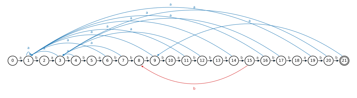
Explicitly, with \(\delta(q,x) = \sigma(P_q x)\) computed by COMPUTE-TRANSITION-FUNCTION, the non-spine transitions with nonzero target are
\begin{equation*} \begin{aligned} &\delta(q,\texttt{a}) = 1 \quad \text{for } q \in \{1,3,6,9,11,14,16,19\},\\ &\delta(q,\texttt{a}) = 3 \quad \text{for } q \in \{4,7,12,17,20\},\\ &\delta(21,\texttt{a}) = 9, \qquad \delta(15,\texttt{b}) = 8, \end{aligned} \end{equation*}
and all remaining non-spine transitions go to state \(0\): namely \(\delta(q,\texttt{b}) = 0\) for \(q \in \{0,2,5,8,10,13,18,21\}\). For example \(\delta(15,\texttt{b}) = 8\) because \(P_{15}\texttt{b} = \texttt{ababbabbababbab}\,\texttt{b}\) ends in \(P_8 = \texttt{ababbabb}\) and in no longer prefix of \(P\), and \(\delta(21,\texttt{a}) = 9\) because \(P\texttt{a}\) ends in \(P_9 = \texttt{ababbabba}\).
Call a pattern \(P\) nonoverlappable if \(P_k \sqsupset P_q\) holds only when \(k = 0\) or \(k = q\). Describe the state-transition diagram of the string-matching automaton for a nonoverlappable pattern \(P[1\,..\,m]\).
Apart from the spine edges \(q \to q+1\) labelled \(P[q+1]\) (\(0 \le q < m\)), every edge goes back to state \(1\) if its label is \(P[1]\) and to state \(0\) otherwise; that is, for every state \(q\) and character \(a\),
\begin{equation*} \delta(q,a) = \begin{cases} q+1 & \text{if } q < m \text{ and } a = P[q+1],\\ 1 & \text{otherwise, if } a = P[1],\\ 0 & \text{otherwise.} \end{cases} \end{equation*}
Indeed, let \(k = \delta(q,a) = \sigma(P_q a)\) for a non-spine pair \((q,a)\), and suppose \(k \ge 2\). Then \(P_k \sqsupset P_q a\) gives \(P[k] = a\) and \(P_{k-1} \sqsupset P_q\) with \(k - 1 \ne 0\), so nonoverlappability forces \(k - 1 = q\). If \(q = m\) this says \(k = m+1\), impossible; if \(q < m\) it says \(P[q+1] = P[k] = a\), so \((q,a)\) is a spine pair, a contradiction. Hence \(k \in \{0,1\}\), and \(k = 1\) exactly when \(P_1 \sqsupset P_q a\), i.e. when \(a = P[1]\).
Given two patterns \(P[1\,..\,m]\) and \(P^{\prime}[1\,..\,m^{\prime}]\), explain how to build a finite automaton that finds every occurrence of either of them in a text, using as few states as you can.
Use as states the set \(S\) of all prefixes of \(P\) or of \(P^{\prime}\), and send state \(x\) on character \(a\) to \(\sigma_S(xa)\), the longest suffix of \(xa\) that lies in \(S\); a state is accepting when it has \(P\) or \(P^{\prime}\) as a suffix. This automaton has
\begin{equation*} |S| = m + m^{\prime} + 1 - \ell \end{equation*}
states, where \(\ell\) is the length of the longest common prefix of \(P\) and \(P^{\prime}\) (the two prefix chains share exactly \(P_0, \dots, P_\ell\)).
TWO-PATTERN-AUTOMATON(P, P', Sigma)
1 S = { P_q : 0 <= q <= m } union { P'_q : 0 <= q <= m' }
2 for each string x in S
3 for each character a in Sigma
4 y = xa
5 while y is not in S
6 remove the first character of y
7 delta(x, a) = y
8 accept(x) = (P is a suffix of x) or (P' is a suffix of x)
9 return delta and accept
The loop of lines 5-6 stops because the empty string is in \(S\), and it tries the suffixes of \(xa\) in decreasing length, so \(\delta(x,a) = \sigma_S(xa)\). The text is then scanned as in FINITE-AUTOMATON-MATCHER, reporting position \(i\) whenever the state after \(T[i]\) is accepting.
Because \(S\) is closed under taking prefixes, the proof of Lemma 32.3 goes through verbatim with \(\sigma_S\) in place of \(\sigma\): if \(r = \sigma_S(wa)\) is nonempty then \(r = r^{\prime}a\) with \(r^{\prime} \in S\) and \(r^{\prime} \sqsupset w\), so \(|r^{\prime}| \le |\sigma_S(w)|\) and \(r \sqsupset \sigma_S(w)a\) by Lemma 32.1; conversely \(\sigma_S(w)a \sqsupset wa\). Hence
\begin{equation*} \sigma_S(wa) = \sigma_S(\sigma_S(w)\,a) \quad \text{for every string } w \text{ and character } a, \end{equation*}
and induction on \(i\) exactly as in Theorem 32.4 shows that the state after reading \(T_i\) is \(\sigma_S(T_i)\). Finally \(P \sqsupset T_i\) iff \(P \sqsupset \sigma_S(T_i)\): one direction is transitivity of \(\sqsupset\), and for the other, \(P \in S\) forces \(|P| \le |\sigma_S(T_i)|\), and both are suffixes of \(T_i\), so Lemma 32.1 applies. The same holds for \(P^{\prime}\), so position \(i\) is reported exactly when an occurrence of \(P\) or \(P^{\prime}\) ends there.
There are \(|S||\Sigma|\) transitions, each found by at most \(m + m^{\prime} + 1\) membership tests costing \(O(m + m^{\prime})\) each (compare \(y\) with the prefix of \(P\) and of \(P^{\prime}\) of length \(|y|\)), so preprocessing takes \(O((m+m^{\prime})^3|\Sigma|)\) time, and matching takes \(\Theta(n)\) time, one transition per text character. If even fewer states are wanted, standard DFA minimization can merge equivalent states of \(S\) (for \(P = \texttt{ab}\), \(P^{\prime} = \texttt{b}\) the states \(\texttt{ab}\) and \(\texttt{b}\) behave identically).
Let \(P\) be a pattern that may contain gap characters \(\diamond\), each matching an arbitrary (possibly empty) string, as in Exercise 32.1-4. Show how to construct a finite automaton that finds an occurrence of \(P\) in a text \(T\) in \(O(n)\) matching time, where \(n = |T|\).
Chain together the string-matching automata of the gap-free pieces of \(P\), jumping to the start of the next piece’s automaton as soon as the current piece is matched. Split \(P\) at its gap characters, discard the empty pieces, and let \(Q_1, \dots, Q_k\) be the remaining ones in order, of lengths \(m_1, \dots, m_k \ge 1\), with string-matching automata \(\delta_1, \dots, \delta_k\). The states are the pairs \((j,q)\) with \(1 \le j \le k\), \(0 \le q < m_j\), plus one absorbing accepting state \(F\), so there are \(m_1 + \cdots + m_k + 1 \le m + 1\) states.
GAP-AUTOMATON(P, Sigma)
1 split P at its gap characters; let Q_1, ..., Q_k be the nonempty pieces
2 for j = 1 to k
3 delta_j = COMPUTE-TRANSITION-FUNCTION(Q_j, Sigma)
4 for q = 0 to m_j - 1
5 for each character a in Sigma
6 r = delta_j(q, a)
7 if r < m_j
8 delta((j, q), a) = (j, r)
9 elseif j < k
10 delta((j, q), a) = (j + 1, 0)
11 else delta((j, q), a) = F
12 delta(F, a) = F for every a in Sigma
13 if k == 0 then start = F else start = (1, 0)
14 return delta, start, and the accepting set {F}
Running FINITE-AUTOMATON-MATCHER with this \(\delta\) and stopping on the first entry into \(F\) reports an occurrence of \(P\) ending at that position.
Since each \(\diamond\) matches any string, \(P\) occurs ending at position \(e\) iff there are positions \(e_1 < \cdots < e_k = e\) with \(Q_j\) ending at \(e_j\) and \(e_j - m_j \ge e_{j-1}\) (put \(e_0 = 0\)): the pieces occur in order without overlapping. Define the greedy positions \(g_0 = 0\) and \(g_j\) = the least \(i\) such that \(Q_j\) ends at \(i\) and \(i - m_j \ge g_{j-1}\).
(i) The automaton enters phase \(j\), in state \((j,0)\), right after reading \(T[g_{j-1}]\), and leaves it right after reading \(T[g_j]\). Indeed, inside phase \(j\) it runs \(\delta_j\) on \(T[g_{j-1}+1\,..\,n]\) from state \(0\), so by Theorem 32.4 it first reaches \(m_j\) at the least \(i\) for which \(Q_j\) is a suffix of \(T[g_{j-1}+1\,..\,i]\), which is \(g_j\).
(ii) The \(g_j\) themselves satisfy the conditions above, so \(P\) occurs ending at \(g_k\); and for any occurrence \(e_1 < \cdots < e_k\), induction gives \(g_j \le e_j\): if \(g_{j-1} \le e_{j-1}\) then \(e_j - m_j \ge e_{j-1} \ge g_{j-1}\), so \(e_j\) is a candidate in the definition of \(g_j\).
Hence the automaton enters \(F\) exactly at the least position at which some occurrence of \(P\) ends, and never enters \(F\) if \(P\) does not occur. (When \(k = 0\), \(P\) matches the empty string and the start state is \(F\).)
Matching makes one table lookup per text character, so it takes \(\Theta(n) = O(n)\) time; preprocessing costs \(O(\sum_j m_j^3 |\Sigma|) = O(m^3|\Sigma|)\) by the bound for COMPUTE-TRANSITION-FUNCTION.
32.4 The Knuth-Morris-Pratt algorithm
Find the prefix function \(\pi\) of the pattern \(P = \texttt{ababbabbabbababbabb}\).
The pattern has length \(m = 19\), and running COMPUTE-PREFIX-FUNCTION gives
| \(i\) | 1 | 2 | 3 | 4 | 5 | 6 | 7 | 8 | 9 | 10 | 11 | 12 | 13 | 14 | 15 | 16 | 17 | 18 | 19 |
|---|---|---|---|---|---|---|---|---|---|---|---|---|---|---|---|---|---|---|---|
| \(P[i]\) | a | b | a | b | b | a | b | b | a | b | b | a | b | a | b | b | a | b | b |
| \(\pi[i]\) | 0 | 0 | 1 | 2 | 0 | 1 | 2 | 0 | 1 | 2 | 0 | 1 | 2 | 3 | 4 | 5 | 6 | 7 | 8 |
For instance, \(\pi[18] = 7\) and \(P[8] = \texttt{b} = P[19]\), so \(\pi[19] = 8\) by Corollary 32.7: \(P_{19}\) ends in \(P_8 = \texttt{ababbabb}\).
Bound the size of the set \(\pi^*[q]\) from above as a function of \(q\), and give an example showing that the bound is tight.
\(|\pi^*[q]| \le q\), with equality for the pattern \(P = \texttt{a}^q\).
Since \(\pi[k] < k\) for every \(k \ge 1\), the iterates satisfy
\begin{equation*} q > \pi[q] > \pi^{(2)}[q] > \cdots > \pi^{(t)}[q] = 0 , \end{equation*}
so \(\pi^*[q]\) consists of \(t\) distinct integers from \(\{0, 1, \ldots, q-1\}\), whence \(t \le q\).
For \(P = \texttt{a}^q\) every prefix \(P_k\) with \(k < q\) is a suffix of \(P_q\), so by Lemma 32.5
\begin{equation*} \pi^*[q] = \{k : k < q \text{ and } P_k \sqsupset P_q\} = \{0, 1, \ldots, q-1\}, \end{equation*}
which has exactly \(q\) elements (concretely \(\pi[k] = k-1\) for all \(k\)).
Let \(P\) have length \(m\) and \(T\) length \(n\). Describe how the occurrences of \(P\) in \(T\) can be read off from the prefix function \(\pi\) of the concatenated string \(PT\) (of length \(m+n\)).
Writing \(S = PT\), the shift \(s\) (\(0 \le s \le n-m\)) is valid exactly when \(m \in \pi^*[2m+s]\), where \(\pi\) is the prefix function of \(S\); this membership is tested for all \(s\) in \(\Theta(m+n)\) total time via the auxiliary array
\begin{equation*} \mu[q] = \text{the largest element of } \pi^*[q] \text{ that is } \le m . \end{equation*}
Correctness. The prefix \(S_m\) of \(S\) is \(P\), and \(S_{2m+s}\) ends in \(S[m+s+1 \,..\, 2m+s] = T[s+1 \,..\, s+m]\). Since \(m < 2m+s\), Lemma 32.5 (applied to the pattern \(S\)) gives
\begin{equation*} m \in \pi^*[2m+s] \iff P \sqsupset S_{2m+s} \iff T[s+1 \,..\, s+m] = P . \end{equation*}
Clearly \(\mu[q] = m\) iff \(m \in \pi^*[q]\). So shift \(s\) is valid iff \(\mu[2m+s] = m\).
Computing \(\mu\). As \(\pi^*[q] = \{\pi[q]\} \cup \pi^*[\pi[q]]\) and \(\pi[q] < q\),
\begin{equation*} \mu[q] = \begin{cases} \pi[q] & \text{if } \pi[q] \le m, \\ \mu[\pi[q]] & \text{if } \pi[q] > m, \end{cases} \end{equation*}
so after COMPUTE-PREFIX-FUNCTION\((S)\), which takes \(\Theta(m+n)\), one pass over \(q = 1, \ldots, m+n\) fills \(\mu\) in \(O(1)\) per entry, and the occurrences are the shifts \(s\) with \(\mu[2m+s] = m\).
Method (2): if a symbol not in \(\Sigma\) is inserted between \(P\) and \(T\), then \(\pi[q] \le m\) for all \(q\), and shift \(s\) is valid iff \(\pi[2m+1+s] = m\).
Show, by aggregate analysis, that KMP-MATCHER runs in \(\Theta(n)\) time.
The value \(q\) rises by at most \(n\) in total, and each execution of line 7 lowers it, so line 7 runs at most \(n\) times overall.
In detail: \(q = 0\) at line 4, and \(q\) increases only in line 9, by \(1\), at most once per iteration of the for loop of line 5, so its total increase is at most \(n\). Each execution of line 7 (where \(q > 0\)) and of line 12 (where \(q = m\)) replaces \(q\) by \(\pi[q] < q\), a decrease of at least \(1\), and \(q \ge 0\) throughout. Hence
\begin{equation*} \begin{aligned} \#\{\text{executions of line 7}\} &\le \text{total decrease of } q \\ &\le \text{total increase of } q \le n . \end{aligned} \end{equation*}
The while test of line 6 is evaluated at most once more than its body per for-iteration, i.e. at most \(2n\) times, and lines 8–12 cost \(O(1)\) per iteration. So lines 4–12 take \(O(n)\), and \(\Omega(n)\) since the for loop makes \(n\) iterations. Line 3 costs \(\Theta(m)\) (shown in the text), which is \(O(n)\) because \(m \le n\) in any meaningful instance. Thus KMP-MATCHER runs in \(\Theta(n)\) time.
Show, using a potential function, that KMP-MATCHER runs in \(\Theta(n)\) time.
Take the potential \(\Phi = q\); every for-loop iteration then has amortized cost at most \(2\).
Charge one unit for the fixed work of an iteration of the for loop (line 5, the final test of line 6, lines 8–12) and one unit per execution of line 7. Consider iteration \(i\), in which line 7 runs \(c_i\) times and line 12 runs \(\ell_i \in \{0, 1\}\) times; its actual cost is \(1 + c_i + \ell_i\). Each execution of line 7 or line 12 replaces \(q\) by \(\pi[q] < q\), lowering \(\Phi\) by at least \(1\), and line 9 raises \(\Phi\) by at most \(1\), so
\begin{equation*} \begin{aligned} \hat c_i &= (1 + c_i + \ell_i) + (\Phi_i - \Phi_{i-1}) \\ &\le (1 + c_i + \ell_i) + (1 - c_i - \ell_i) = 2 . \end{aligned} \end{equation*}
As \(\Phi_0 = 0\) and \(\Phi_i \ge 0\) for all \(i\), the total actual cost of the loop is
\begin{equation*} \sum_{i=1}^n (1 + c_i + \ell_i) = \sum_{i=1}^n \hat c_i - \Phi_n + \Phi_0 \le 2n . \end{equation*}
It is also at least \(n\), so lines 4–12 take \(\Theta(n)\); with the \(\Theta(m) = O(n)\) cost of line 3 (for \(m \le n\)), KMP-MATCHER runs in \(\Theta(n)\) time.
Modify KMP-MATCHER by using \(\pi^{\prime}\) instead of \(\pi\) in line 7 (line 12 keeps \(\pi\)), where for \(q = 1, 2, \ldots, m-1\) the function \(\pi^{\prime}\) is defined recursively by
\begin{equation*} \pi^{\prime}[q] = \begin{cases} 0 & \text{if } \pi[q] = 0, \\ \pi^{\prime}[\pi[q]] & \text{if } \pi[q] \ne 0 \text{ and } P[\pi[q]+1] = P[q+1], \\ \pi[q] & \text{if } \pi[q] \ne 0 \text{ and } P[\pi[q]+1] \ne P[q+1]. \end{cases} \end{equation*}
Explain why the modified matcher is still correct, and in what sense the change is an improvement.
\(\pi^{\prime}[q]\) is the largest \(k \in \pi^*[q]\) with \(k = 0\) or \(P[k+1] \ne P[q+1]\), so the jump in line 7 skips only states whose next character equals \(P[q+1]\), which has just been seen to differ from \(T[i]\); the modified matcher therefore reaches exactly the same state as the original after every while loop, while never comparing \(T[i]\) against a character already known to mismatch.
Characterization. Induct on \(q\) (note \(\pi[q] < q\), so \(\pi^{\prime}[\pi[q]]\) is defined in the middle case). Using \(\pi^*[q] = \{\pi[q]\} \cup \pi^*[\pi[q]]\):
(i) \(\pi[q] = 0\): \(\pi^*[q] = \{0\}\), so the maximum is \(0\).
(ii) \(r = \pi[q] \ne 0\), \(P[r+1] = P[q+1]\): \(r\) is excluded, and by induction \(\pi^{\prime}[r]\) is the largest \(k \in \pi^*[r]\) with \(k = 0\) or \(P[k+1] \ne P[r+1] = P[q+1]\).
(iii) \(r = \pi[q] \ne 0\), \(P[r+1] \ne P[q+1]\): the largest element \(r\) of \(\pi^*[q]\) qualifies.
Correctness. Fix an iteration with text character \(a = T[i]\) and starting state \(q_0 \le m-1\) (after line 12, \(q = \pi[m] < m\)). By the text’s analysis the original while loop runs down \(\pi^*[q_0]\) and stops at
\begin{equation*} k^* = \max\{k \in \{q_0\} \cup \pi^*[q_0] : k = 0 \text{ or } P[k+1] = a\} . \end{equation*}
Claim: the modified loop keeps \(q \in \{q_0\} \cup \pi^*[q_0]\) and \(q \ge k^*\). Initially true. If the loop body runs, then \(q > 0\) and \(P[q+1] \ne a\), so \(q > k^*\) and \(k^* \in \pi^*[q]\) (the elements of \(\pi^*[q_0]\) below \(q\) are exactly \(\pi^*[q]\)). Every \(k \in \pi^*[q]\) with \(k > \pi^{\prime}[q]\) has \(k > 0\) and \(P[k+1] = P[q+1] \ne a\), so \(k \ne k^*\); hence \(k^* \le \pi^{\prime}[q] \in \pi^*[q]\), preserving the claim. The loop exits only when \(q = 0\) or \(P[q+1] = a\), i.e. \(q \le k^*\), so \(q = k^*\), the same state as the original. Lines 8–12 are unchanged, so the outputs coincide. Line 12 must keep \(\pi\): at \(q = m\) no character has mismatched, \(P[m+1]\) does not exist, and \(\pi^{\prime}[m]\) is undefined.
Improvement. \(\pi^{\prime}\) is computed from \(\pi\) in \(\Theta(m)\) time by the recurrence, in increasing \(q\). Each modified while loop visits a subset of the states the original visits, so it never does more comparisons, and it avoids every redundant one. The asymptotic bound stays \(\Theta(n)\), but the work on a single text character can drop sharply: for \(P = \texttt{a}^m\) we have \(\pi^{\prime}[q] = 0\) for all \(q\), so on \(T = \texttt{a}^{m-1}\texttt{b}\) the original executes line 7 \(m-1\) times on the final character, the modified matcher once.
Design a linear-time algorithm that decides whether a text \(T\) is a cyclic rotation of another string \(T^{\prime}\). (For instance, the strings arc and car are cyclic rotations of one another.)
\(T^{\prime}\) is a rotation of \(T\) exactly when \(|T| = |T^{\prime}|\) and \(T^{\prime}\) occurs in the doubled text \(TT\); test this with one KMP run with pattern \(T^{\prime}\) and text \(TT\).
IS-ROTATION(T, T')
1 m = T.length
2 if T'.length != m
3 return FALSE
4 if m == 0
5 return TRUE
6 let T2[1..2m] be T concatenated with T
7 return KMP-MATCHER(T2, T') finds at least one valid shift
Correctness. Say \(|T| = |T^{\prime}| = m\). If \(T = xy\) and \(T^{\prime} = yx\), then \(TT = x\,(yx)\,y\), so \(T^{\prime}\) occurs in \(TT\) at shift \(|x|\). Conversely, if \(T^{\prime} = TT[s+1 \,..\, s+m]\) for some shift \(0 \le s \le m\), put \(x = T[1\,..\,s]\) and \(y = T[s+1\,..\,m]\); then \(TT = xyxy\) and
\begin{equation*} T^{\prime} = TT[s+1\,..\,s+m] = yx , \end{equation*}
so \(T^{\prime}\) is a cyclic rotation of \(T\). Hence the algorithm answers correctly (KMP-MATCHER reports exactly the valid shifts).
Running time. Line 6 takes \(\Theta(m)\); COMPUTE-PREFIX-FUNCTION on \(T^{\prime}\) runs in \(\Theta(m)\) and the matching loop on a text of length \(2m\) runs in \(\Theta(2m)\) (Section 32.4’s aggregate analyses), so the total is \(\Theta(m)\), linear in the input size.
Design an \(O(m\,|\Sigma|)\)-time algorithm that computes the transition function \(\delta\) of the string-matching automaton for a given pattern \(P[1\,..\,m]\). (Hint: show that \(\delta(q, a) = \delta(\pi[q], a)\) whenever \(q = m\) or \(P[q+1] \ne a\).)
Compute \(\pi\) with COMPUTE-PREFIX-FUNCTION, then fill \(\delta\) row by row in increasing \(q\), using \(\delta(q,a) = q+1\) when \(q < m\) and \(P[q+1] = a\), \(\delta(0,a) = 0\) otherwise for \(q = 0\), and the hint’s identity \(\delta(q,a) = \delta(\pi[q],a)\) otherwise; row \(\pi[q] < q\) is already filled.
FAST-COMPUTE-TRANSITION-FUNCTION(P, Sigma)
1 m = P.length
2 pi = COMPUTE-PREFIX-FUNCTION(P)
3 for q = 0 to m
4 for each character a in Sigma
5 if q < m and P[q+1] == a
6 delta(q, a) = q + 1
7 elseif q == 0
8 delta(q, a) = 0
9 else delta(q, a) = delta(pi[q], a)
10 return delta
Proof of the hint. Let \(1 \le q \le m\) with \(q = m\) or \(P[q+1] \ne a\), and let \(k = \sigma(P_q a) = \delta(q,a)\) (equation (32.4)). First \(k \le q\): \(k = q+1\) is impossible, since \(q+1 > m\) or \(P_{q+1} = P_q P[q+1] \not\sqsupset P_q a\); and \(k \le q+1\) always. Now:
(i) \(\sigma(P_{\pi[q]} a) \le k\): \(P_{\pi[q]} \sqsupset P_q\) gives \(P_{\pi[q]} a \sqsupset P_q a\), so any prefix of \(P\) that is a suffix of \(P_{\pi[q]} a\) is a suffix of \(P_q a\).
(ii) \(\sigma(P_{\pi[q]} a) \ge k\): trivial if \(k = 0\). If \(k \ge 1\), then \(P_k \sqsupset P_q a\) gives \(P[k] = a\) and \(P_{k-1} \sqsupset P_q\) with \(k - 1 < q\), so \(k - 1 \le \pi[q]\) by the definition of \(\pi\). Both \(P_{k-1}\) and \(P_{\pi[q]}\) are suffixes of \(P_q\), so \(P_{k-1} \sqsupset P_{\pi[q]}\) by Lemma 32.1, and
\begin{equation*} P_k = P_{k-1}\, a \sqsupset P_{\pi[q]}\, a . \end{equation*}
Hence \(\delta(q,a) = k = \sigma(P_{\pi[q]} a) = \delta(\pi[q], a)\).
Correctness. By induction on \(q\), rows \(0, \dots, q-1\) are correct when row \(q\) is filled. Line 6 is correct since \(P_{q+1} \sqsupset P_q a\) is the longest possible. For \(q = 0\) and \(P[1] \ne a\), no nonempty prefix of \(P\) equals \(a\), so \(\sigma(a) = 0\) (line 8). Otherwise \(q \ge 1\) and (\(q = m\) or \(P[q+1] \ne a\)), so line 9 is correct by the hint and the induction hypothesis, as \(\pi[q] < q\).
Running time. Line 2 takes \(\Theta(m)\) (Section 32.4), and lines 3-9 do \(O(1)\) work for each of the \((m+1)|\Sigma|\) pairs \((q,a)\), for a total of \(O(m\,|\Sigma|)\).
Problems for Chapter 32
String matching based on repetition factors: write \(y^i\) for the string \(y\) concatenated with itself \(i\) times, so for instance \((\mathtt{ab})^3 = \mathtt{ababab}\). A string \(x \in \Sigma^*\) has repetition factor \(r\) if \(x = y^r\) for some \(y \in \Sigma^*\) and some \(r > 0\); let \(\rho(x)\) be the largest such \(r\).
(a) Give an efficient algorithm that, given a pattern \(P[1 \,..\, m]\), computes \(\rho(P_i)\) for every \(i = 1, 2, \ldots, m\). What is its running time?
(b) For a pattern \(P[1 \,..\, m]\) put \(\rho^*(P) = \max_{1 \le i \le m} \rho(P_i)\). Show that when \(P\) is drawn uniformly at random from the binary strings of length \(m\), the expected value of \(\rho^*(P)\) is \(O(1)\).
(c) Argue that the following algorithm (due to Galil and Seiferas) correctly reports every occurrence of \(P\) in a text \(T[1 \,..\, n]\) and runs in time \(O(\rho^*(P)\, n + m)\):
REPETITION-MATCHER(P, T)
1 m = P.length
2 n = T.length
3 k = 1 + rho*(P)
4 q = 0
5 s = 0
6 while s <= n - m
7 if T[s + q + 1] == P[q + 1]
8 q = q + 1
9 if q == m
10 print "Pattern occurs with shift" s
11 if q == m or T[s + q + 1] != P[q + 1]
12 s = s + max(1, ceil(q / k))
13 q = 0
(a) Compute the prefix function \(\pi\) and set \(p_i = i - \pi[i]\); then \(\rho(P_i) = i/p_i\) if \(p_i \mid i\) and \(\rho(P_i) = 1\) otherwise. This takes \(\Theta(m)\) time.
REPETITION-FACTORS(P)
1 m = P.length
2 pi = COMPUTE-PREFIX-FUNCTION(P)
3 let rho[1..m] be a new array
4 for i = 1 to m
5 p = i - pi[i]
6 if i mod p == 0
7 rho[i] = i / p
8 else rho[i] = 1
9 return rho
Call \(d\) a period of a string \(x\) of length \(i\) if \(x[j] = x[j+d]\) for \(1 \le j \le i - d\); \(d\) is a period exactly when \(x_{i-d} \sqsupset x\), so by the definition of \(\pi\) (Section 32.4) the smallest period of \(P_i\) is \(p_i = i - \pi[i]\). Also \(P_i = y^r\) with \(|y| = d\) if and only if \(d \mid i\), \(r = i/d\) and \(d\) is a period of \(P_i\).
If \(p_i \mid i\) then \(P_i = (P_{p_i})^{i/p_i}\), and any \(P_i = y^r\) has \(|y|\) a period, so \(|y| \ge p_i\) and \(r \le i/p_i\); hence \(\rho(P_i) = i/p_i\). If \(p_i \nmid i\), suppose \(P_i = y^r\) with \(r \ge 2\) and \(d = |y| \le i/2\). Then \(p_i < d\) (as \(p_i \ne d\)) and \(p_i + d \le i\), and \(d - p_i\) is again a period:
\begin{equation*} \begin{aligned} j \le i-d &: \quad P[j] = P[j+d] = P[j+d-p_i], \\ i-d < j \le i-d+p_i &: \quad P[j] = P[j-p_i] = P[j-p_i+d], \end{aligned} \end{equation*}
using \(j > i - d \ge p_i\) in the second line. The pair \((p_i, d-p_i)\) again has sum \(d \le i\), so iterating this subtraction (Euclid’s algorithm, Section 31.2) shows \(\gcd(p_i, d)\) is a period. Minimality of \(p_i\) gives \(p_i = \gcd(p_i,d) \mid d \mid i\), a contradiction; so \(\rho(P_i) = 1\).
Lines 1-2 take \(\Theta(m)\) by the analysis of COMPUTE-PREFIX-FUNCTION in Section 32.4, and the loop takes \(\Theta(m)\), for \(\Theta(m)\) in total.
(b) \(E[\rho^*(P)] \le 3\). If \(\rho(P_i) \ge r\), say \(P_i = y^{r^{\prime}}\) with \(r^{\prime} \ge r\) and \(|y| = d\), then \(rd \le m\) and \(P_{rd} = (P_d)^r\). Given the first \(d\) bits, this event fixes the next \((r-1)d\) bits, so it has probability \(2^{-(r-1)d}\). A union bound over \(d\) gives, for \(r \ge 2\),
\begin{equation*} \Pr\{\rho^*(P) \ge r\} \le \sum_{d \ge 1} 2^{-(r-1)d} = \frac{1}{2^{r-1}-1} \le \frac{1}{2^{r-2}} . \end{equation*}
Then by equation (C.25),
\begin{equation*} E[\rho^*(P)] = \sum_{r \ge 1} \Pr\{\rho^*(P) \ge r\} \le 1 + \sum_{r \ge 2} 2^{-(r-2)} = 3 = O(1). \end{equation*}
(c) Correctness. For a fixed value of \(s\), lines 7-8 extend \(q\) while characters match. Line 11 fires exactly when \(q\) equals the length \(q_s\) of the longest prefix of \(P\) matching \(T\) at shift \(s\) (the test after line 8 looks ahead at the next character), and line 10 prints exactly when \(q_s = m\). Since \(q < m\) whenever line 7 runs, every index stays in range (\(s + q + 1 \le s + m \le n\)), and the “or” short-circuits when \(q = m\). Every shift examined is therefore reported correctly. It remains to show that no valid shift is skipped. Suppose \(s + t\) is valid for some \(0 < t < \lceil q_s/k \rceil\), so \(kt < q_s\). For \(t < j \le q_s\), both \(T[s+j] = P[j]\) (match at \(s\)) and \(T[s+j] = P[j-t]\) (match at \(s+t\)) hold. So \(t\) is a period of \(P_{q_s}\), hence of its prefix \(P_{kt}\), which has length divisible by \(t\). Thus \(P_{kt} = (P_t)^k\) with \(kt \le m\), and
\begin{equation*} \rho^*(P) \ge \rho(P_{kt}) \ge k = 1 + \rho^*(P), \end{equation*}
a contradiction.
Running time. Each iteration of the while loop either increments \(q\) or ends the current shift, so shift \(s\) costs at most \(q_s + 1\) iterations. Its step is \(\Delta_s = \max(1, \lceil q_s/k \rceil) \ge q_s/k\). The steps sum to at most \((n - m) + m = n\): every examined shift is \(\le n - m\), and each step is at most \(\lceil m/k \rceil \le m\). Hence
\begin{equation*} \sum_s (q_s + 1) \le \sum_s (k \Delta_s + 1) \le kn + (n - m + 1) = O(\rho^*(P)\, n). \end{equation*}
Line 3 costs \(O(m)\) by part (a), so the total is \(O(\rho^*(P)\, n + m)\).
Chapter 33: Computational Geometry
33.1 Line-segment properties
Show that if the cross product \(p_1 \times p_2\) is positive, then the vector \(p_1\) is clockwise from the vector \(p_2\) with respect to the origin \((0,0)\), and that if \(p_1 \times p_2\) is negative, then \(p_1\) is counterclockwise from \(p_2\).
In polar form \(p_1\times p_2=r_1r_2\sin(\beta-\alpha)\), so its sign is the sign of the counterclockwise angle from \(p_1\) to \(p_2\) measured in \((-\pi,\pi]\). Indeed, write \(p_1=r_1(\cos\alpha,\sin\alpha)\) and \(p_2=r_2(\cos\beta,\sin\beta)\) with \(r_1,r_2>0\) (a zero vector gives cross product \(0\)). Then
\begin{equation*} \begin{aligned} p_1\times p_2 &= x_1y_2-x_2y_1 = r_1r_2(\cos\alpha\sin\beta-\cos\beta\sin\alpha)\\ &= r_1r_2\sin(\beta-\alpha). \end{aligned} \end{equation*}
Here “\(p_1\) is clockwise from \(p_2\)” means that \(p_1\) is obtained from the direction of \(p_2\) by a clockwise rotation through an angle strictly between \(0\) and \(\pi\) (the lightly shaded half-plane of Figure 33.1(b)), i.e. \(\beta-\alpha\in(0,\pi)\pmod{2\pi}\); counterclockwise is the mirror condition \(\alpha-\beta\in(0,\pi)\pmod{2\pi}\).
(i) If \(p_1\times p_2>0\), then \(\sin(\beta-\alpha)>0\), i.e. \(\beta-\alpha\in(0,\pi)\pmod{2\pi}\), so \(p_2\) is a counterclockwise rotation of (the direction of) \(p_1\) by less than \(\pi\): \(p_1\) is clockwise from \(p_2\).
(ii) If \(p_1\times p_2<0\), then \(\sin(\alpha-\beta)>0\), i.e. \(\alpha-\beta\in(0,\pi)\pmod{2\pi}\), so \(p_1\) is a counterclockwise rotation of \(p_2\) by less than \(\pi\): \(p_1\) is counterclockwise from \(p_2\). \(\blacksquare\)
Professor van Pelt suggests that in line 1 of ON-SEGMENT\((p_i,p_j,p_k)\) it suffices to test only the \(x\)-coordinate, i.e. to check just \(\min(x_i,x_j)\le x_k\le\max(x_i,x_j)\). Show that the professor is wrong.
The \(x\)-test fails for vertical segments. Take \(p_i=(0,0)\), \(p_j=(0,1)\), \(p_k=(0,5)\): the point \(p_k\) is colinear with \(\overline{p_ip_j}\) (as ON-SEGMENT assumes), and \(\min(0,0)\le 0\le\max(0,0)\), so the professor’s test returns TRUE, yet \(p_k\) is not on the segment since \(y_k=5>\max(y_i,y_j)=1\).
The error propagates to SEGMENTS-INTERSECT: for the disjoint segments \(\overline{p_1p_2}\) with \(p_1=(0,0)\), \(p_2=(0,1)\) and \(\overline{p_3p_4}\) with \(p_3=(0,5)\), \(p_4=(0,6)\), all four \(d_k\) are \(0\), and line 7 calls ON-SEGMENT\((p_3,p_4,p_1)\), whose \(x\)-only test (\(0\le 0\le 0\)) succeeds, so the procedure wrongly returns TRUE.
The polar angle of a point \(p_1\) with respect to an origin \(p_0\) is the angle, in ordinary polar coordinates, of the vector \(p_1-p_0\). For instance, relative to \((2,4)\) the point \((3,5)\) has polar angle \(45^\circ=\pi/4\) (vector \((1,1)\)), and the point \((3,3)\) has polar angle \(315^\circ=7\pi/4\) (vector \((1,-1)\)). Give pseudocode that sorts a sequence \(\langle p_1,p_2,\ldots,p_n\rangle\) of \(n\) points by polar angle with respect to a given origin \(p_0\), in \(O(n\lg n)\) time, using cross products to compare angles.
Translate so that \(p_0\) is the origin, split the plane into the half-open upper half \(H_0\) (angles in \([0,\pi)\)) and lower half \(H_1\) (angles in \([\pi,2\pi)\)), and merge sort with the comparator “\(a\) precedes \(b\) iff \(a\) lies in an earlier half, or both lie in the same half and \(a\times b>0\)”. We assume no \(p_i\) equals \(p_0\) (its polar angle is undefined).
HALF(v)
1 if v.y > 0 or (v.y == 0 and v.x > 0)
2 return 0 // angle in [0, pi)
3 else return 1 // angle in [pi, 2 pi)
POLAR-LESS(a, b) // a, b already translated by p0
1 if HALF(a) != HALF(b)
2 return HALF(a) < HALF(b)
3 return a.x * b.y - b.x * a.y > 0
POLAR-SORT(p, n, p0)
1 for i = 1 to n
2 q[i] = (p[i].x - p0.x, p[i].y - p0.y)
3 MERGE-SORT(q, 1, n), comparing keys with POLAR-LESS
4 for i = 1 to n
5 p[i] = (q[i].x + p0.x, q[i].y + p0.y)
6 return p
Correctness: it suffices that POLAR-LESS\((a,b)\) holds exactly when \(\theta(a)<\theta(b)\), where \(\theta\in[0,2\pi)\) is the polar angle; then it is the “\(<\)” of a total preorder and MERGE-SORT sorts by \(\theta\). Line 2 of HALF tests exactly \(\theta(v)\in[0,\pi)\), so different halves are ordered correctly by line 2 of POLAR-LESS. If \(a,b\) lie in the same half, then \(|\theta(b)-\theta(a)|<\pi\), and by the computation in Exercise 33.1-1
\begin{equation*} a\times b=|a|\,|b|\sin\bigl(\theta(b)-\theta(a)\bigr)>0 \iff \theta(a)<\theta(b), \end{equation*}
while \(a\times b=0\) forces \(\theta(a)=\theta(b)\) (equal angles are ties, and neither precedes the other).
Running time: translation is \(\Theta(n)\), each comparison is \(O(1)\) arithmetic with no division or trigonometry, and MERGE-SORT makes \(O(n\lg n)\) comparisons, so the total is \(O(n\lg n)\).
Given a set of \(n\) points in the plane, show how to decide in \(O(n^2\lg n)\) time whether some three of them are colinear.
For each point \(p_i\), sort the other \(n-1\) points by the direction (modulo \(\pi\)) of the line through them and \(p_i\), and look for two adjacent points in sorted order whose directions coincide. Concretely, each vector \(v=p_j-p_i\) is replaced by \(-v\) if it lies in the lower half \(H_1\) of Exercise 33.1-3, so that all vectors have angles in \([0,\pi)\); on such vectors “\(a\) precedes \(b\) iff \(a\times b>0\)” orders by angle (Exercise 33.1-3).
ANY-COLINEAR(P, n)
1 for i = 1 to n
2 Q = empty array
3 for j = 1 to n, j != i
4 v = P[j] - P[i]
5 if v.y < 0 or (v.y == 0 and v.x < 0)
6 v = -v
7 append v to Q
8 MERGE-SORT Q so that a precedes b when a x b > 0
9 for k = 1 to n - 2
10 if Q[k] x Q[k+1] == 0
11 return TRUE
12 return FALSE
Correctness: three distinct points \(p_i,p_j,p_k\) are colinear iff \((p_j-p_i)\times(p_k-p_i)=0\), i.e. iff the two vectors are parallel or antiparallel, i.e. iff their normalized versions \(v_j,v_k\) (both with angle in \([0,\pi)\)) have the same angle, i.e. \(v_j\times v_k=0\) (negation does not change \(\vert a\times b\vert\)). (i) If line 11 is reached, then \(Q[k]\) and \(Q[k+1]\) come from two points \(p_j,p_k\) with \(p_i,p_j,p_k\) colinear. (ii) Conversely, if \(p_i,p_j,p_k\) are colinear, then in iteration \(i\) the vectors \(v_j,v_k\) have equal angle; since \(Q\) is sorted by angle, all vectors of that angle form a contiguous block of length \(\ge 2\), and the first two entries of that block are adjacent with cross product \(0\), so line 11 is reached (in iteration \(i\) or earlier).
Running time: each of the \(n\) iterations of line 1 spends \(O(n)\) on lines 2–7 and 9–11 and \(O(n\lg n)\) on the sort (constant-time cross-product comparisons), for a total of \(n\cdot O(n\lg n)=O(n^2\lg n)\).
A polygon is a closed, piecewise-linear curve in the plane: a chain of straight-line segments (its sides) that ends where it starts; a point where two consecutive sides meet is a vertex. A simple polygon (the default assumption) does not cross itself; it encloses its interior, the curve itself is its boundary, and the rest of the plane is its exterior. A simple polygon is convex if the segment joining any two points of its boundary or interior stays within the boundary or interior. A vertex of a convex polygon is never a convex combination of two distinct points of the boundary or interior.
Professor Amundsen proposes the following test of whether the sequence \(\langle p_0,p_1,\ldots,p_{n-1}\rangle\) lists the consecutive vertices of a convex polygon: answer “yes” if the set of angles \(\{\angle p_ip_{i+1}p_{i+2}: i=0,1,\ldots,n-1\}\) (indices mod \(n\)) does not contain both a left turn and a right turn, and “no” otherwise. Show that this linear-time method can give a wrong answer, and modify it so that it is always correct and still runs in linear time.
The professor accepts a pentagram; the fix is to require every turn to be strictly in one direction and the boundary to wind around exactly once, which is detected in linear time by counting the local minima of the vertices in \((y,x)\)-lexicographic order.
Counterexample. The convex pentagon with vertices \((0,0),(2,0),(3,2),(1,3),(-1,2)\), visited every second vertex, gives
\begin{equation*} \langle p_0,\ldots,p_4\rangle=\langle(0,0),(3,2),(-1,2),(2,0),(1,3)\rangle . \end{equation*}
With \(e_i=p_{i+1}-p_i\), the five cross products \(e_i\times e_{i+1}\) are \(8,8,7,6,7\), all positive, so every turn is a left turn and the professor says “yes”; but the sides \(\overline{p_0p_1}\) and \(\overline{p_2p_3}\) cross (at \((1,2/3)\)), so the curve is a self-intersecting star, not a convex polygon.
Fixed method. Write \(q\prec r\) when \((q_y,q_x)<(r_y,r_x)\) lexicographically, so that \(e_i\) lies in the lower half \(H_1\) of Exercise 33.1-3 iff \(p_{i+1}\prec p_i\).
CONVEX-VERTICES(p, n)
1 if n < 3
2 return "no"
3 if (p[1] - p[0]) x (p[2] - p[1]) < 0
4 reverse p // right turns become left turns
5 m = 0
6 for i = 0 to n - 1 // indices mod n
7 if (p[i+1] - p[i]) x (p[i+2] - p[i+1]) <= 0
8 return "no"
9 if p[i+1] precedes both p[i] and p[i+2] in (y, x) order
10 m = m + 1
11 if m == 1 return "yes" else return "no"
Every iteration is \(O(1)\), so the method runs in \(\Theta(n)\) time. After line 4 we may assume (counterclockwise orientation) that a correct answer “yes” means all turns are left turns; lines 7–8 reject a zero cross product, which is right, because then \(p_i,p_{i+1},p_{i+2}\) are colinear and one of them is a convex combination of the other two (or two coincide), so it is not a vertex.
Winding count. Let all turns be strict left turns, so \(e_{i+1}\) is \(e_i\) rotated counterclockwise by \(\delta_i\in(0,\pi)\), and the total turning is \(\sum_i\delta_i=2\pi w\) for an integer \(w\ge 1\). The accumulated direction passes through angle \(0\pmod{2\pi}\) at step \(i\) iff \(e_i\in H_1\) and \(e_{i+1}\in H_0\) (a step of less than \(\pi\) leaves \(H_1\) for \(H_0\) exactly when it crosses \(2\pi\)), i.e. iff \(p_{i+1}\prec p_i\) and \(p_{i+1}\prec p_{i+2}\). So \(m=w\).
Sufficiency (\(m=1\) gives a convex polygon). Fix \(i\) and let \(n_i\) be the left normal of \(e_i\). Going around from \(p_{i+1}\), the directions \(\theta_{i+1}<\theta_{i+2}<\cdots<\theta_{i-1}\) increase within \((\theta_i,\theta_i+2\pi)\) since \(w=1\), and the height of the next vertex above the line of \(e_i\) changes by
\begin{equation*} e_j\cdot n_i=|e_j|\sin(\theta_j-\theta_i), \end{equation*}
which is positive while \(\theta_j<\theta_i+\pi\) and negative afterwards (zero at \(\theta_i+\pi\)). The height starts at \(0\) at \(p_{i+1}\), first increases (the \(e_{i+1}\) step is positive), then never increases again, and returns to \(0\) at \(p_i\) by a negative last step (\(e_{i-1}\)); hence every vertex other than \(p_i,p_{i+1}\) lies strictly to the left of the line through \(p_i,p_{i+1}\). Consequently: the \(p_k\) are distinct; each \(p_{i+1}\) is an extreme point of the convex hull \(\mathrm{conv}(P)\) (all other points lie in the wedge left of the lines of \(e_i\) and \(e_{i+1}\), whose apex \(p_{i+1}\) is an extreme point because the turn is strict); and each \(\overline{p_ip_{i+1}}\) is an edge of the hull (its line supports \(\mathrm{conv}(P)\) and touches it only along that segment). The hull boundary is a simple closed polygon with exactly these \(n\) vertices and \(n\) edges, and the \(n\) distinct sides \(\overline{p_ip_{i+1}}\) are all among them, so the given polygon is the boundary of \(\mathrm{conv}(P)\): convex, with vertices in the given order.
Necessity (a convex polygon listed counterclockwise gives \(m=1\)). All turns are strict left turns, as noted above. A local minimum \(p_{i+1}\) (that is, \(p_{i+1}\prec p_i\) and \(p_{i+1}\prec p_{i+2}\)) is the global \(\prec\)-minimum: every point of the polygon lies left of the supporting lines of \(e_i\) and \(e_{i+1}\), i.e. in the cone \(p_{i+1}+\{a(-e_i)+be_{i+1}:a,b\ge 0\}\); both generators are \(\succ 0\), and the set \(\{v\succ 0\}\) is closed under addition and positive scaling, so every other point of the cone is \(\succ p_{i+1}\). The global minimum is unique and is a local minimum, so \(m=1\).
Hence CONVEX-VERTICES answers “yes” exactly when the sequence lists the consecutive vertices of a convex polygon (in either orientation, by line 4).
For a point \(p_0=(x_0,y_0)\), the right horizontal ray from \(p_0\) is \(\{p_i=(x_i,y_i): x_i\ge x_0 \text{ and } y_i=y_0\}\), the points due right of \(p_0\) together with \(p_0\). Show how to decide in \(O(1)\) time whether the right horizontal ray from \(p_0\) meets a segment \(\overline{p_1p_2}\), by reducing to the question of whether two line segments intersect.
Truncate the ray just past the segment: with
\begin{equation*} q=\bigl(\max(x_0,x_1,x_2)+1,\;y_0\bigr), \end{equation*}
the ray meets \(\overline{p_1p_2}\) iff SEGMENTS-INTERSECT\((p_0,q,p_1,p_2)\) returns TRUE.
RAY-INTERSECTS(p0, p1, p2)
1 q = (max(p0.x, p1.x, p2.x) + 1, p0.y)
2 return SEGMENTS-INTERSECT(p0, q, p1, p2)
Correctness: \(\overline{p_0q}\) is a nondegenerate segment (\(x_q>x_0\)) contained in the ray, so an intersection with \(\overline{p_0q}\) is one with the ray. Conversely, every point of \(\overline{p_1p_2}\) is a convex combination of \(p_1,p_2\) and so has \(x\)-coordinate at most \(\max(x_1,x_2)<x_q\); hence a common point \(r\) of the ray and the segment satisfies \(x_0\le x_r<x_q\) and \(y_r=y_0\), i.e. \(r\in\overline{p_0q}\). So the two questions have the same answer, and SEGMENTS-INTERSECT decides the second correctly (Section 33.1).
Running time: line 1 is a constant number of comparisons and one addition, and SEGMENTS-INTERSECT is \(O(1)\), so the test takes \(O(1)\) time.
To decide whether a point \(p_0\) lies in the interior of a simple (not necessarily convex) polygon \(P\), one can take any ray from \(p_0\) and check that it meets the boundary of \(P\) an odd number of times while \(p_0\) itself is not on the boundary. Show how to decide in \(\Theta(n)\) time whether \(p_0\) is in the interior of an \(n\)-vertex polygon \(P\). (Hint: use Exercise 33.1-6, and make sure the algorithm is correct when the ray passes through a vertex of the polygon and when it overlaps a side.)
Reject if \(p_0\) lies on some side; otherwise cast the right horizontal ray from \(p_0\) and count, with the half-open convention “a vertex with \(y_i = y_0\) counts as below the ray”, the sides \(\overline{ab}\) (with \(a.y \le b.y\)) satisfying \(a.y \le y_0 < b.y\) and lying to the right of \(p_0\); answer “interior” iff the count is odd.
POINT-IN-POLYGON(P, p0) // P = <p_0, ..., p_{n-1}>, p0 = (x0, y0)
1 inside = FALSE
2 for i = 0 to n - 1
3 a = p_i
4 b = p_{(i+1) mod n}
5 if DIRECTION(a, b, p0) == 0 and ON-SEGMENT(a, b, p0)
6 return FALSE // p0 is on the boundary
7 if a.y > b.y
8 exchange a with b // now a is the lower endpoint
9 if a.y <= y0 < b.y and DIRECTION(a, b, p0) < 0
10 inside = not inside
11 return inside
Lines 5-6 are the boundary test used inside SEGMENTS-INTERSECT, so the procedure returns FALSE exactly when \(p_0\) is on the boundary. Suppose now \(p_0\) is on no side, so its distance \(\delta\) to the boundary is positive, and let \(\varepsilon\) satisfy \(0 < \varepsilon < \delta\) and \(\varepsilon < |y_i - y_0|\) for every \(y_i \ne y_0\) (and small enough as needed below). Put \(p_0^{\prime} = (x_0, y_0 + \varepsilon)\). The segment \(\overline{p_0 p_0^{\prime}}\) misses the boundary, so \(p_0\) is interior iff \(p_0^{\prime}\) is. The right horizontal ray \(r^{\prime}\) from \(p_0^{\prime}\) passes through no vertex (no \(y_i\) equals \(y_0 + \varepsilon\)), hence overlaps no side and crosses each side it meets transversally at an interior point of that side; so the parity criterion applies to \(r^{\prime}\) with no degeneracies, and each side is counted at most once. A side \(\overline{ab}\) (\(a.y \le b.y\)) meets the line \(y = y_0 + \varepsilon\) iff
\begin{equation*} a.y < y_0 + \varepsilon < b.y \iff a.y \le y_0 < b.y , \end{equation*}
by the choice of \(\varepsilon\); in particular horizontal sides (both endpoints at the same height, e.g. a side overlapping the original ray) are never counted, and a vertex on the original ray is handled through its two sides like any other point below the line. For such a side, the crossing point is to the right of \(p_0^{\prime}\) iff \(p_0^{\prime}\) is to the left of the directed segment \(a \to b\), i.e. iff \((p_0^{\prime} - a)\times(b - a) < 0\) (this is the test of Exercise 33.1-6 for \(r^{\prime}\)). This cross product is continuous in \(\varepsilon\), and at \(\varepsilon = 0\) it equals DIRECTION\((a, b, p_0) \ne 0\) (a zero value with \(a.y \le y_0 < b.y\) would put \(p_0\) on the side, which lines 5-6 excluded); so for small \(\varepsilon\) its sign is that of DIRECTION\((a, b, p_0)\), which is exactly the test in line 9. Hence line 10 toggles once per crossing of \(r^{\prime}\) with the boundary, and the procedure returns TRUE iff that number is odd, iff \(p_0^{\prime}\), equivalently \(p_0\), is interior.
Running time: the loop makes exactly \(n\) iterations, each a constant number of cross products and comparisons (DIRECTION and ON-SEGMENT are \(O(1)\)), so the time is \(\Theta(n)\).
Show how to compute, in \(\Theta(n)\) time, the area of a simple (not necessarily convex) polygon with \(n\) vertices. (Exercise 33.1-5 gives the definitions concerning polygons.)
With vertices \(p_0, p_1, \ldots, p_{n-1}\) listed in boundary order and indices taken mod \(n\), the area is
\begin{equation*} A(P) = \frac{1}{2}\left| \sum_{i=0}^{n-1} p_i \times p_{i+1} \right| = \frac{1}{2}\left| \sum_{i=0}^{n-1} (x_i y_{i+1} - x_{i+1} y_i) \right| . \end{equation*}
POLYGON-AREA(P) // P = <p_0, ..., p_{n-1}>
1 s = 0
2 for i = 0 to n - 1
3 j = (i + 1) mod n
4 s = s + p_i.x * p_j.y - p_j.x * p_i.y
5 return |s| / 2
Correctness: since \(P\) is simple, its boundary is a simple closed piecewise-linear curve enclosing the interior \(R\), so Green’s theorem gives, with the boundary traversed counterclockwise,
\begin{equation*} \operatorname{area}( R) = \frac{1}{2}\oint_{\partial R} (x\,dy - y\,dx) , \end{equation*}
and traversing it clockwise only flips the sign; the vertex order is one of these two traversals, hence the absolute value. On side \(i\), parametrize \(p = p_i + t(p_{i+1} - p_i)\), \(0 \le t \le 1\), with \(\Delta x = x_{i+1} - x_i\), \(\Delta y = y_{i+1} - y_i\):
\begin{equation*} \begin{aligned} \int_{\text{side } i} (x\,dy - y\,dx) &= \int_0^1 \bigl[(x_i + t\Delta x)\Delta y - (y_i + t\Delta y)\Delta x\bigr]\,dt \\ &= x_i \Delta y - y_i \Delta x = x_i y_{i+1} - x_{i+1} y_i = p_i \times p_{i+1} . \end{aligned} \end{equation*}
Summing over the \(n\) sides gives the formula.
Running time: the loop performs exactly \(n\) iterations of \(O(1)\) arithmetic, so the time is \(\Theta(n)\).
33.2 Determining whether any pair of segments intersects
Show that a set of \(n\) line segments can have \(\Theta(n^2)\) intersections.
A grid of \(\lfloor n/2\rfloor\) horizontal and \(\lceil n/2\rceil\) steep segments has \(\lfloor n/2\rfloor\lceil n/2\rceil = \Theta(n^2)\) intersections, and no set can have more than \(\binom n2\).
Upper bound: two segments meet in at most one point unless they are colinear and overlap, so counting intersecting pairs there are at most \(\binom n2 = O(n^2)\) of them.
Lower bound: let \(k=\lfloor n/2\rfloor\) and take
\begin{equation*} \begin{aligned} h_i &= \overline{(0,i)\,(2n,i)}, && i=1,\dots,k,\\ v_j &= \overline{(2j,0)\,(2j+1,n)}, && j=1,\dots,n-k . \end{aligned} \end{equation*}
The \(h_i\) lie on distinct parallel lines, as do the \(v_j\) (all of slope \(n\)), so no two segments of the same family meet. The segment \(v_j\) crosses height \(y=i\in[0,n]\) at \(x=2j+i/n\in[2j,2j+1]\subset[0,2n]\), so \(h_i\) and \(v_j\) meet at the point \((2j+i/n,\,i)\); these \(k(n-k)\) points are pairwise distinct. Hence there are
\begin{equation*} k(n-k)=\lfloor n/2\rfloor\lceil n/2\rceil\ \ge\ \frac{n^2-1}{4}=\Omega(n^2) \end{equation*}
intersections.
Segments \(a\) and \(b\), neither vertical, are comparable at \(x\). Show how to decide in \(O(1)\) time whether \(a \succcurlyeq_x b\) or \(b \succcurlyeq_x a\). (Hint from the book: if \(a\) and \(b\) do not intersect, cross products suffice; if they do intersect, which cross products can detect, addition, subtraction and multiplication still suffice, with no division. In the sweep application one may in any case stop as soon as \(a\) and \(b\) are found to intersect.)
Compare the heights of \(a\) and \(b\) on the sweep line after clearing the (positive) denominators: with \(a=\overline{p_1p_2}\), \(b=\overline{p_3p_4}\), \(p_i=(x_i,y_i)\), \(x_1<x_2\), \(x_3<x_4\) (strict because neither segment is vertical), put
\begin{equation*} \begin{aligned} A &= \bigl((x_2-x_1)\,y_1+(x-x_1)(y_2-y_1)\bigr)(x_4-x_3),\\ B &= \bigl((x_4-x_3)\,y_3+(x-x_3)(y_4-y_3)\bigr)(x_2-x_1). \end{aligned} \end{equation*}
Then \(a\succcurlyeq_x b \iff A\ge B\) and \(b\succcurlyeq_x a\iff B\ge A\) (both hold exactly when \(a\) and \(b\) meet on the sweep line).
Indeed \(a\) meets the line at height \(y_a(x)=y_1+(x-x_1)(y_2-y_1)/(x_2-x_1)\) and similarly for \(b\), and
\begin{equation*} A-B=(x_2-x_1)(x_4-x_3)\,\bigl(y_a(x)-y_b(x)\bigr) \end{equation*}
with \((x_2-x_1)(x_4-x_3)>0\), so the sign of \(A-B\) is the sign of \(y_a(x)-y_b(x)\), which by definition decides \(\succcurlyeq_x\). Computing \(A\) and \(B\) takes a constant number of additions, subtractions and multiplications (exact on integer coordinates), so the test is \(O(1)\).
In ANY-SEGMENTS-INTERSECT the comparison is made at the \(x\)-coordinate of an endpoint, say \(x=x_3\); then the formula collapses to a single cross product:
\begin{equation*} A-B=-(x_4-x_3)\,\bigl((p_2-p_1)\times(p_3-p_1)\bigr), \end{equation*}
so \(a\succcurlyeq_{x_3} b\) iff \((p_2-p_1)\times(p_3-p_1)\le 0\), that is, iff \(p_3\) lies on or below the line through \(p_1p_2\) (clockwise from \(p_2\) with respect to \(p_1\), Section 33.1).
Professor Mason proposes changing ANY-SEGMENTS-INTERSECT so that, rather than returning when it finds an intersection, it prints the intersecting segments and goes on to the next iteration of the for loop. He calls this PRINT-INTERSECTING-SEGMENTS and claims it prints every intersection, in left-to-right order. Professor Dixon says the idea is wrong. Who is right? Does PRINT-INTERSECTING-SEGMENTS always find the leftmost intersection first? Does it always find all the intersections?
Professor Dixon is right: the procedure need not report the leftmost intersection first, and it need not report every intersection.
The procedure only tests pairs that are consecutive in \(T\) at an endpoint event, and it tests them at that event, possibly long before the intersection point is reached; and \(T\) is never reordered at crossings, so after the first crossing its order is stale.
(i) Not left to right. Take \(a=\overline{(0,0)(10,0)}\), \(b=\overline{(1,1)(9,-1)}\), \(c=\overline{(2,5)(4,3)}\), \(d=\overline{(2,3)(4,5)}\). At the event \((1,1)\) segment \(b\) is inserted next to \(a\) and the pair \(a,b\) is printed, although they meet at \((5,0)\); the pair \(c,d\), which meets at \((3,4)\), is printed only at the event \(x=2\). So the leftmost intersection is not reported first.
(ii) Not all intersections. Take \(a=\overline{(1,1)(5,-1)}\), \(b=\overline{(0,0)(10,0)}\), \(c=\overline{(2,-1)(6,1)}\). Then \(a\cap b=(3,0)\), \(b\cap c=(4,0)\) and \(a\cap c=(3.5,-0.25)\). Running the procedure:
| event | action | \(T\) (top to bottom) | printed |
|---|---|---|---|
| \((0,0)\) left of \(b\) | insert \(b\) | \(b\) | |
| \((1,1)\) left of \(a\) | insert \(a\) | \(a,b\) | \(a,b\) |
| \((2,-1)\) left of \(c\) | insert \(c\) | \(a,b,c\) | \(b,c\) |
| \((5,-1)\) right of \(a\) | delete \(a\) (no segment above it) | \(b,c\) | |
| \((6,1)\) right of \(c\) | delete \(c\) (no segment below it) | \(b\) | |
| \((10,0)\) right of \(b\) | delete \(b\) |
Segments \(a\) and \(c\) are never consecutive in \(T\) at an event, because \(b\) separates them at every event, so the intersection \(a\cap c\) is never printed.
Give an \(O(n\lg n)\)-time algorithm that decides whether a polygon with \(n\) vertices is simple.
Check in \(O(n)\) time that consecutive sides meet only at their shared vertex, then run ANY-SEGMENTS-INTERSECT on the \(n\) sides, counting two sides as intersecting only when they are not consecutive; the polygon is simple iff no such pair is reported.
With vertices \(v_0,\dots,v_{n-1}\) (indices mod \(n\)) and sides \(e_i=\overline{v_iv_{i+1}}\), call a pair of sides bad if they intersect and are not consecutive. Two segments with a common endpoint \(v_i\) meet somewhere else iff they are colinear and point the same way from \(v_i\), so lines 1-4 below test exactly whether consecutive sides meet only at their shared vertex. Line 5 applies the shear \((x,y)\mapsto(x+\varepsilon y,y)\) with \(\varepsilon=\tfrac12\min\{|\Delta x/\Delta y|\}\) over the sides with \(\Delta x\ne0\ne\Delta y\) (\(\varepsilon=1\) if there are none). It is an affine bijection, so it preserves which sides intersect, and afterwards no side is vertical, since \(|\varepsilon\Delta y|<|\Delta x|\) whenever \(\Delta x\ne0\). In the sweep, \(T\) compares sides by their height at the sweep line (Exercise 33.2-2), and a tie at a common point is broken by slope, the steeper side going above, which is the order just to the right.
SIMPLE-POLYGON(v[0..n-1]) // indices mod n
1 for i = 0 to n-1
2 if v[i] == v[i+1] return FALSE
3 if (v[i-1]-v[i]) x (v[i+1]-v[i]) == 0 and
(v[i-1]-v[i]) . (v[i+1]-v[i]) > 0
4 return FALSE // consecutive sides overlap
5 shear all vertices so that no side is vertical
6 S = {e[0], ..., e[n-1]}
7 run ANY-SEGMENTS-INTERSECT(S), where in lines 6 and 9
"s intersects t" means SEGMENTS-INTERSECT(s,t) and
s, t are not consecutive sides
8 return FALSE if it returns TRUE, else TRUE
Correctness. The polygon is simple iff consecutive sides meet only at their shared vertex and there is no bad pair. Lines 1-4 decide the first condition, and a reported pair is always bad, so it remains to show: if lines 1-4 pass and a bad pair exists, line 7 reports one. Let \(p\) be the leftmost point lying on a bad pair, taking the lowest if there are several.
A side \(e_i\) has a consecutive side through \(p\) only if \(p\) is the common vertex of the two sides, and \(p\) cannot be both \(v_i\) and \(v_{i+1}\). So on the set \(C\) of sides through any point, the relation “consecutive” is a matching, and if \(|C|\ge3\) some two sides in \(C\) are not consecutive, which gives a bad pair. Hence each point before \(p\) in \((x,y)\)-lexicographic order lies on at most two sides, and if it lies on two, they are consecutive sides sharing it as an endpoint. Pairs that are not bad never cross.
Look at the moment \(M\) after all events with \(x<p_x\) and all left-endpoint events at \(x=p_x\) with \(y\le p_y\) have been processed; this is a prefix of the event order of line 2 of the book’s procedure, which puts left endpoints first at equal \(x\). Then \(T\) holds exactly the sides whose left endpoint is lexicographically at most \(p\) and whose right endpoint has \(x\ge p_x\); in particular \(T\supseteq C\). Between two sides of \(T\) there is no crossing before \(p\), and any tie at an insertion is a single comparison with the unique other side through that point, settled by slope. So, as in the book’s proof, \(T\) is ordered (weakly) by height on the line \(x=p_x\). The sides through \(p\) are exactly the sides of \(T\) at height \(p_y\) there, so \(C\) forms a contiguous block of \(T\) with \(|C|\ge2\). By the matching remark this block contains two adjacent members \(a,b\) that form a bad pair: if \(|C|=2\), \(C\) itself is the bad pair through \(p\); if \(|C|\ge3\), the two adjacent pairs around a middle element cannot both be matched.
Now \(a\) and \(b\) are consecutive in \(T\) at \(M\). They became consecutive either when the later of them was inserted, and then lines 6-7 test it against both of its neighbours, or when a side between them was deleted, and then lines 9-10 test them. Either way the bad pair is reported, unless the procedure has already stopped with an earlier report.
Running time: lines 1-6 take \(O(n)\). Line 7 is ANY-SEGMENTS-INTERSECT on \(n\) segments, each comparison and test still costs \(O(1)\), so it runs in \(O(n\lg n)\). The total is \(O(n\lg n)\).
Give an \(O(n\lg n)\)-time algorithm that decides whether two simple polygons, having \(n\) vertices between them, intersect.
The polygons \(P\) and \(Q\) (each taken as boundary plus interior) intersect iff some side of \(P\) meets some side of \(Q\), or a vertex of \(P\) lies inside \(Q\), or a vertex of \(Q\) lies inside \(P\). The first condition is tested by an \(O(n\lg n)\) sweep, the other two in \(O(n)\) each.
(1) Boundaries. Run the sweep of Exercise 33.2-4 (after the same shear) on all \(n\) sides of \(P\) and \(Q\), where a pair now counts as bad iff the two sides intersect and come from different polygons. Since \(P\) and \(Q\) are simple, two intersecting sides of the same polygon are consecutive sides that meet only at their shared vertex. So the pairs that are not bad are exactly those the proof of Exercise 33.2-4 allows: on the sides through any point they form a matching, and they never cross. That proof therefore applies word for word, and the sweep reports a bad pair iff the boundaries \(\partial P\) and \(\partial Q\) meet.
(2) Containment. If the boundaries are disjoint, test one vertex of \(P\) for lying in the interior of \(Q\), and one vertex of \(Q\) for lying in the interior of \(P\), using Exercise 33.1-7. Answer “intersect” iff one of the tests succeeds.
Correctness of (2): a positive test clearly gives a common point. Conversely, suppose \(\partial P\cap\partial Q=\emptyset\). The plane minus \(\partial Q\) splits into the open sets \(\operatorname{int}Q\) and \(\operatorname{ext}Q\), and \(\partial P\) is connected, so (i) \(\partial P\subseteq\operatorname{int}Q\) or (ii) \(\partial P\subseteq\operatorname{ext}Q\); likewise (i’) \(\partial Q\subseteq\operatorname{int}P\) or (ii’) \(\partial Q\subseteq\operatorname{ext}P\). (i) Every vertex of \(P\) is inside \(Q\), and the test succeeds. (i’) Symmetric. (ii) and (ii’) Then \(P\cap Q=\emptyset\). Suppose \(z\in P\cap Q\). Since \(\partial P\subseteq\operatorname{ext}Q\), \(z\notin\partial P\), so \(z\in\operatorname{int}P\). The region \(Q\) is connected and meets both \(\operatorname{int}P\) (at \(z\)) and \(\operatorname{ext}P\) (along \(\partial Q\)), so it meets \(\partial P\). That point is not on \(\partial Q\), so it lies in \(\operatorname{int}Q\), contradicting \(\partial P\subseteq\operatorname{ext}Q\).
Running time: (1) costs \(O(n\lg n)\) by Exercise 33.2-4, and (2) costs \(O(n)\) by Exercise 33.1-7, so the total is \(O(n\lg n)\).
A disk is a circle together with its interior, given by its center and its radius; two disks intersect if they share at least one point. Give an \(O(n\lg n)\)-time algorithm that decides whether some two of \(n\) given disks intersect.
Sweep exactly as in ANY-SEGMENTS-INTERSECT. Disk \(d\), with center \((x_d,y_d)\) and radius \(r_d\), enters at \(x=x_d-r_d\) and leaves at \(x=x_d+r_d\). The status \(T\) is a red-black tree keyed by the center height \(y_d\), ties broken by index, and only disks adjacent in \(T\) are tested, by \((x_d-x_e)^2+(y_d-y_e)^2\le(r_d+r_e)^2\).
ANY-DISKS-INTERSECT(D)
1 T = empty red-black tree keyed by (y_d, index of d)
2 sort the 2n events (x_d - r_d, 0, d) and (x_d + r_d, 1, d)
lexicographically (entries before exits at equal x)
3 for each event (x, e, d) in sorted order
4 if e == 0
5 INSERT(T, d)
6 if ABOVE(T,d) or BELOW(T,d) exists and meets d
7 return TRUE
8 else
9 if ABOVE(T,d), BELOW(T,d) both exist and meet
10 return TRUE
11 DELETE(T, d)
12 return FALSE
Correctness. A TRUE answer exhibits two intersecting disks. Conversely, let disks \(a\) and \(b\) share a point \(p\), and let \(M\) be the moment after every event before \((p_x,1,\cdot)\) has been processed, that is, after all exits with \(x<p_x\) and all entries with \(x\le p_x\). Then \(T\) holds exactly the disks \(d\) whose \(x\)-range contains \(p_x\), including \(a\) and \(b\). On the line \(x=p_x\) each such \(d\) cuts out an interval \(I_d\) centred at \(y_d\), and
\begin{equation*} I_d\cap I_e=\emptyset,\ I_d \text{ above } I_e \ \Rightarrow\ y_d\ge\min I_d>\max I_e\ge y_e. \tag{\(*\)} \end{equation*}
Among all pairs in \(T\) whose intervals meet (\(a,b\) is one, because \(p_y\in I_a\cap I_b\)), choose one, \(d\) below \(e\), with as few elements of \(T\) between them as possible. Suppose some \(c\) lies strictly between them in \(T\), so \(y_d\le y_c\le y_e\). By minimality \(I_c\) meets neither \(I_d\) nor \(I_e\). Then (\(*\)) puts \(I_c\) above \(I_d\) (otherwise \(y_c<y_d\)) and below \(I_e\) (otherwise \(y_c>y_e\)), which separates \(I_d\) from \(I_e\), a contradiction. So \(d\) and \(e\) are consecutive in \(T\) at \(M\), and the disks intersect, at a point of the line \(x=p_x\).
Every pair that is consecutive in \(T\) became so at some event: either when the later of the two was inserted (tested in lines 6-7) or when a disk between them was deleted (tested in lines 9-10). So the pair \(d,e\) was tested before \(M\), and the procedure returned TRUE at that test, if not earlier.
Running time: sorting takes \(O(n\lg n)\). There are \(2n\) iterations, each doing \(O(1)\) red-black-tree operations at \(O(\lg n)\) apiece (Chapter 13) and \(O(1)\) arithmetic tests. The total is \(O(n\lg n)\).
You are given \(n\) line segments among which there are \(k\) intersections in total. Show how to report all \(k\) of them in \(O((n+k)\lg n)\) time.
Sweep as in ANY-SEGMENTS-INTERSECT, but make the event-point schedule dynamic: besides the \(2n\) endpoints it holds every intersection point of two segments that have been adjacent in \(T\), and at an intersection event we report the point and swap the two segments in \(T\) (the Bentley-Ottmann sweep). We work under the section’s assumptions (no vertical segment, no three segments through a point) and assume further that no endpoint lies on another segment, so that \(k\) counts crossing pairs. The schedule \(Q\) is a red-black tree keyed lexicographically on \((x,y)\), which supports EXTRACT-MIN, INSERT and a membership test in logarithmic time.
PRINT-ALL-INTERSECTIONS(S)
1 T = empty red-black tree (sweep-line status)
2 Q = red-black tree of the 2n endpoints, keyed on (x, y)
3 while Q is not empty
4 p = EXTRACT-MIN(Q)
5 if p is the left endpoint of a segment s
6 INSERT(T, s)
7 CHECK(ABOVE(T, s), s, p); CHECK(s, BELOW(T, s), p)
8 elseif p is the right endpoint of a segment s
9 a = ABOVE(T, s); b = BELOW(T, s)
10 DELETE(T, s); CHECK(a, b, p)
11 else // p is where s, above t just left of p, meets t
12 print p, s, t
13 swap the positions of s and t in T
14 CHECK(ABOVE(T, t), t, p); CHECK(s, BELOW(T, s), p)
CHECK(u, v, p)
1 if u and v exist and meet at a point q later than p in (x, y) order
2 if q is not already in Q
3 insert q into Q, labelled with u and v
Taking events in lexicographic \((x,y)\) order is the same as sweeping with a line turned through an infinitesimal angle, so in the argument we may assume that all event points have distinct \(x\)-coordinates. The invariant is: after the event at abscissa \(x_e\) has been processed, \(T\) holds exactly the segments that cross the sweep line just to the right of \(x_e\), ordered by height there, and \(Q\) holds every remaining endpoint together with every intersection point to the right of \(x_e\) of each pair that is adjacent in \(T\).
Initialization: \(T=\emptyset\) and \(Q\) holds all the endpoints.
Maintenance: an insertion, a deletion, or a swap at a crossing (which is a genuine swap of order, by the lemma below) makes \(T\) correct for the next interval. The only pairs that become adjacent are \((s,\mathrm{ABOVE})\) and \((s,\mathrm{BELOW})\) at a left endpoint, \((a,b)\) at a right endpoint, and the new outer pairs at a swap. CHECK tests exactly these pairs, and nothing is ever deleted from \(Q\).
Lemma: if \(s\) and \(t\) cross at \(q\) and \(e\) is the last event before \(q\), then \(s\) and \(t\) are adjacent in \(T\) after \(e\). Both segments are active on \((x_e,x_q)\), because their left endpoints are events and are not \(q\). Suppose a segment \(u\) lay between them on that interval. Then \(u\) does not end before \(x_q\), since there are no events in between, and \(u\) does not end at \(q\), since endpoints lie on no other segment. By continuity \(u\) passes through \(q\), which puts three segments through one point, a contradiction.
By the lemma and the invariant, every intersection point enters \(Q\) before the sweep reaches it. The membership test lets it enter only once, so it is reported exactly once. Everything reported is a genuine intersection, so the output is exactly the \(k\) intersections, from left to right.
Time: there are \(2n+k\) events. Each one does \(O(1)\) operations on \(T\) (size \(\le n\)) and \(O(1)\) calls to CHECK, each costing \(O(1)\) for the test of Section 33.1 plus \(O(\lg|Q|)\). Since \(|Q|\le 2n+k\le 2n+\binom n2\), we have \(\lg|Q|=O(\lg n)\), and the total is
\begin{equation*} O\bigl((2n+k)\lg n\bigr)=O\bigl((n+k)\lg n\bigr). \end{equation*}
Show that ANY-SEGMENTS-INTERSECT still gives the correct answer when three or more of the segments pass through a common point.
The procedure stays correct: we replace the one step of the book’s proof (page 1026) that uses the assumption, namely that \(a\) and \(b\) become consecutive. The direction “TRUE \(\Rightarrow\) an intersection exists” does not use the assumption, since lines 7 and 10 return only after an actual intersection test succeeds. For the converse we use two facts.
(F1) Every pair of segments that are ever consecutive in \(T\) was tested for intersection when it became consecutive. A pair becomes consecutive only when one of its segments is inserted next to the other, which line 6 tests, or when the segment between them is deleted, which line 9 tests first. Rotations inside the red-black tree do not change the in-order sequence.
(F2) Let \(x^*\) be the least abscissa of an intersection point. While the events at \(x^*\) are being processed, \(T\) is weakly sorted by height on the line \(x=x^*\). Just before the first event at \(x^*\), \(T\) is correctly and strictly ordered on the open strip between the previous event abscissa and \(x^*\), because no intersections lie left of \(x^*\) (this is the book’s statement that “the order given by \(T\) is correct” left of \(p\)). Letting \(x\to x^*\) turns strict inequalities of heights into weak ones. Each later INSERT at \(x^*\) compares heights at \(x^*\), which keeps \(T\) weakly sorted.
Now let \(p\) be an intersection point on \(x=x^*\) and let \(A\) be the set of segments through \(p\), with \(|A|\ge 2\). All left endpoints at \(x^*\) are processed before any right endpoint there. So once those left endpoints are done (if the procedure has not already returned TRUE), \(T\) contains every segment that meets the line \(x=x^*\), and in particular all of \(A\).
Suppose \(c\) lies between two members of \(A\) in \(T\). By (F2) the height of \(c\) at \(x^*\) is squeezed between \(y_p\) and \(y_p\). So \(c\) passes through \(p\), that is, \(c\in A\). Hence \(A\) is a contiguous block of \(T\). As \(|A|\ge2\), two members of \(A\) are consecutive in \(T\), and by (F1) they were tested and the procedure returned TRUE.
Suppose vertical segments are allowed, and ANY-SEGMENTS-INTERSECT handles each one by treating its lower endpoint as a left endpoint and its upper endpoint as a right endpoint. Show that the procedure is then still correct. How must the comparison of Exercise 33.2-2 be modified to allow vertical segments?
The procedure is still correct, provided that in every comparison a vertical segment \(v\) at abscissa \(x_v\) is represented by its lower endpoint \((x_v,y_v^{\mathrm{bot}})\).
On the line \(x=\xi\), give each segment \(s\) meeting that line the key \(k_\xi(s)\) and the interval \(J_\xi(s)\):
\begin{equation*} \begin{aligned} k_\xi(s)&=y_s(\xi),\quad J_\xi(s)=\{y_s(\xi)\} &&\text{for } s \text{ not vertical},\\ k_\xi(v)&=y_v^{\mathrm{bot}},\quad J_\xi(v)=[y_v^{\mathrm{bot}},y_v^{\mathrm{top}}] &&\text{for } v \text{ vertical}, x_v=\xi. \end{aligned} \end{equation*}
Two segments meeting the line \(x=\xi\) intersect on that line iff their intervals overlap. Every comparison made by INSERT happens at the abscissa \(\xi\) of the current event, and with the rule above it compares exactly these keys. A vertical segment is inserted and deleted at events of its own abscissa, so it is never in \(T\) at any other abscissa.
“TRUE \(\Rightarrow\) an intersection exists” holds as before, because the test SEGMENTS-INTERSECT of Section 33.1 is correct for vertical segments too. For the converse, let \(x^*\) be the least abscissa of an intersection point. Fact (F1) of Exercise 33.2-8 holds unchanged, and so does (F2), with “weakly sorted by \(k_{x^*}\)” in place of “weakly sorted by height”. The limiting argument for (F2) involves only non-vertical segments, since every vertical segment at an abscissa \(\xi<x^*\) was deleted at \(\xi\), and there it met nothing, so every comparison made at \(\xi\) agreed with the true order of the non-vertical segments.
All left events at \(x^*\), including the lower endpoints of vertical segments there, are processed before any right event at \(x^*\). So once they are done, \(T=(s_1,\dots,s_m)\) lists, from bottom to top, every segment meeting the line \(x=x^*\), with
\begin{equation*} k_{x^*}(s_1)\le k_{x^*}(s_2)\le\cdots\le k_{x^*}(s_m). \end{equation*}
Some two intervals \(J_{x^*}(s_i)\), \(J_{x^*}(s_j)\) with \(i<j\) overlap. Writing \(J_{x^*}(s_i)=[l_i,h_i]\), sortedness and the overlap give
\begin{equation*} l_i\le l_{i+1}\le l_j\le h_i . \end{equation*}
So \(J_{x^*}(s_{i+1})\) meets \(J_{x^*}(s_i)\), and the consecutive pair \(s_i,s_{i+1}\) intersects. By (F1) that pair was tested and TRUE was returned.
Change to Exercise 33.2-2: segments are now comparable at \(x\) also when one of them is vertical with abscissa \(x\). Comparisons happen only inside INSERT\((T,b)\), where \(b\) is represented by the event point \(q\), its left endpoint (the lower endpoint if \(b\) is vertical). Comparing \(b\) with a segment \(a\) already in \(T\):
(i) \(a=\overline{p_1p_2}\) not vertical, with \(p_1\) its left endpoint: \(b\) is above \(a\) iff \((p_2-p_1)\times(q-p_1)\ge0\). This is the test of Exercise 33.2-2, and it is unchanged when \(b\) is vertical;
(ii) \(a\) vertical: \(b\) is above \(a\) iff \(q_y\ge y_a^{\mathrm{bot}}\).
Each case is one cross product or one comparison, with no division, so it takes \(O(1)\) time.
33.3 Finding the convex hull
In GRAHAM-SCAN, let \(\langle p_1, p_2, \ldots, p_m\rangle\) be the points of \(Q - \{p_0\}\) sorted by polar angle around \(p_0\) (keeping, for each angle, only the point farthest from \(p_0\)). Prove that \(p_1\) and \(p_m\) are both vertices of \(\mathrm{CH}(Q)\).
All of \(Q\) lies in a closed half-plane bounded by the line \(p_0p_1\) and meets that line only in the segment \(\overline{p_0p_1}\), so \(p_1\) is an endpoint of a hull edge; likewise for \(p_m\).
Let \(\theta_q\in[0,\pi)\) be the polar angle of \(q\ne p_0\) around \(p_0\) (page 1031), so \(\theta_1\le\theta_q\le\theta_m\). Define the affine function \(f(x)=(p_1-p_0)\times(x-p_0)\). For \(q\in Q-\{p_0\}\),
\begin{equation*} f(q)=|p_1-p_0|\,|q-p_0|\sin(\theta_q-\theta_1)\ \ge 0, \end{equation*}
because \(\theta_q-\theta_1\in[0,\pi)\), with equality only when \(\theta_q=\theta_1\), i.e. \(q\) is on the ray from \(p_0\) through \(p_1\); by the tie rule of line 2, \(|q-p_0|\le|p_1-p_0|\), so \(q\in\overline{p_0p_1}\). Hence \(f\ge 0\) on \(Q\) and \(Q\cap\{f=0\}\subseteq\overline{p_0p_1}\). Since \(f\) is affine, \(f\ge0\) on \(\mathrm{CH}(Q)\), and a point of \(\mathrm{CH}(Q)\) with \(f=0\) is a convex combination of points of \(Q\) with \(f=0\) only (any weight on a point with \(f>0\) makes \(f>0\)), so \(\mathrm{CH}(Q)\cap\{f=0\}\subseteq\overline{p_0p_1}\).
Now suppose \(p_1=\lambda a+(1-\lambda)b\) with \(a,b\in\mathrm{CH}(Q)\) and \(0<\lambda<1\). Then
\begin{equation*} 0=f(p_1)=\lambda f(a)+(1-\lambda)f(b),\qquad f(a),f(b)\ge 0, \end{equation*}
so \(f(a)=f(b)=0\) and \(a,b\in\overline{p_0p_1}\). As \(p_1\) is an endpoint of this segment, \(a=b=p_1\). Thus \(p_1\) is not a convex combination of other points of \(\mathrm{CH}(Q)\): it is a vertex.
For \(p_m\) repeat the argument with \(g(x)=(x-p_0)\times(p_m-p_0)\), for which \(g(q)=|q-p_0|\,|p_m-p_0|\sin(\theta_m-\theta_q)\ge0\) with equality only on \(\overline{p_0p_m}\) (again by the tie rule).
Suppose a model of computation allows addition, comparison and multiplication, and in it sorting \(n\) numbers requires \(\Omega(n\lg n)\) time. Prove that, in the same model, computing the vertices of the convex hull of \(n\) points, listed in order around the hull, also requires \(\Omega(n\lg n)\) time.
Sorting reduces to ordered convex hull in \(O(n)\) time by lifting each number \(x\) to the parabola point \((x,x^2)\).
The sorting lower bound holds already for inputs of \(n\) distinct numbers (the lower-bound argument, as in Theorem 8.1, only uses inputs that are permutations of distinct values), and for \(n\le 2\) there is nothing to prove; so let \(x_1,\ldots,x_n\) be distinct, \(n\ge3\). Compute \(q_i=(x_i,x_i^2)\) with \(n\) multiplications. For \(a<b<c\),
\begin{equation*} \bigl((b,b^2)-(a,a^2)\bigr)\times\bigl((c,c^2)-(a,a^2)\bigr)=(b-a)(c-a)(c-b)>0 . \end{equation*}
Let \(y_1<y_2<\cdots<y_n\) be the sorted values and \(r_k=(y_k,y_k^2)\). Every cyclically consecutive triple of \(\langle r_1,\ldots,r_n\rangle\) is a left turn: for \((r_{k-1},r_k,r_{k+1})\) this is the display; \((r_{n-1},r_n,r_1)\) and \((r_n,r_1,r_2)\) are cyclic shifts of \((r_1,r_{n-1},r_n)\) and \((r_1,r_2,r_n)\), and a cyclic shift does not change the cross product’s sign. Moreover each \(r_k\) is a vertex of the hull: the line \(y=2y_kx-y_k^2\) passes through \(r_k\) and every other \(q_i\) lies strictly above it, since \(x_i^2-2y_kx_i+y_k^2=(x_i-y_k)^2>0\). In particular the points are not all collinear. So \(\langle r_1,\ldots,r_n\rangle\) is a convex polygon traversed counterclockwise whose vertex set is all of \(\{q_i\}\), and the counterclockwise vertex order of \(\mathrm{CH}(\{q_i\})\) is a cyclic rotation of the sorted order.
Hence: run the hull algorithm on \(q_1,\ldots,q_n\); if it lists the vertices clockwise (one cross product of three consecutive output vertices tells), reverse the list; find the vertex with the smallest \(x\)-coordinate (\(n-1\) comparisons) and read the \(x\)-coordinates cyclically from there. This outputs \(y_1,\ldots,y_n\). If the hull algorithm took \(T(n)\) time, sorting would take \(T(n)+O(n)\), so \(T(n)+O(n)=\Omega(n\lg n)\), i.e. \(T(n)=\Omega(n\lg n)\).
Let \(Q\) be a set of points. Prove that the two points of \(Q\) at maximum distance from each other are both vertices of \(\mathrm{CH}(Q)\).
A non-vertex of the hull is a proper convex combination of two hull points, and strict convexity of squared distance then produces a hull point even farther away, which is impossible.
Let \(p,q\in Q\) realize the maximum distance \(D=|p-q|\); by symmetry it suffices to show \(p\) is a vertex. First, every \(c\in\mathrm{CH}(Q)\) has \(|c-q|\le D\): writing \(c=\sum_i\mu_iq_i\) as a convex combination of points \(q_i\in Q\),
\begin{equation*} |c-q|=\Bigl|\sum_i\mu_i(q_i-q)\Bigr|\le\sum_i\mu_i|q_i-q|\le D . \end{equation*}
Suppose \(p\) is not a vertex. Then \(p\) lies in the interior of \(\mathrm{CH}(Q)\) or in the relative interior of an edge, so \(p=\lambda a+(1-\lambda)b\) for some distinct \(a,b\in\mathrm{CH}(Q)\) and \(0<\lambda<1\). By the identity \(|\lambda u+(1-\lambda)v|^2=\lambda|u|^2+(1-\lambda)|v|^2-\lambda(1-\lambda)|u-v|^2\) with \(u=a-q\), \(v=b-q\),
\begin{equation*} \begin{aligned} D^2=|p-q|^2&=\lambda|a-q|^2+(1-\lambda)|b-q|^2-\lambda(1-\lambda)|a-b|^2\\ &<\max\{|a-q|^2,|b-q|^2\}\le D^2, \end{aligned} \end{equation*}
a contradiction. Hence \(p\), and likewise \(q\), is a vertex of \(\mathrm{CH}(Q)\).
For a polygon \(P\) and a point \(q\) on its boundary, the shadow of \(q\) is the set of points \(r\) for which the whole segment \(\overline{qr}\) lies in \(P\) (on its boundary or in its interior). \(P\) is star-shaped if some point \(p\) in the interior of \(P\) lies in the shadow of every boundary point; the set of all such \(p\) is the kernel of \(P\). (Figure 33.10(a) shows a star-shaped polygon with a kernel point \(p\): the segment from \(p\) to any boundary point \(q\) meets the boundary only at \(q\). Figure 33.10(b) shows a polygon with two boundary points \(q,q^{\prime}\) whose shadows are disjoint, so its kernel is empty.) Given an \(n\)-vertex star-shaped polygon \(P\) by its vertices in counterclockwise order, show how to compute \(\mathrm{CH}(P)\) in \(O(n)\) time.
Run Graham’s stack scan directly on the boundary order, starting from the lowest vertex and wrapping around to it: the vertices are already sorted by angle around a kernel point \(p\), which is all the scan needs.
STAR-HULL(P)
1 let u0 be the vertex of P with minimum y-coordinate,
or the leftmost such vertex in case of a tie
2 let <u0, u1, ..., u(n-1)> be the vertices of P in
counterclockwise order starting at u0; u(n) = u0
3 let S be an empty stack
4 PUSH(u0, S); PUSH(u1, S)
5 for i = 2 to n
6 while S has at least 2 points and NEXT-TO-TOP(S),
TOP(S), u(i) make a nonleft turn
7 POP(S)
8 PUSH(u(i), S)
9 POP(S) // discard the second copy of u0
10 return S
Fix a kernel point \(p\) and write \(o(a,b,c)=(b-a)\times(c-a)\). For each edge \(\overline{ab}\) of \(P\), \(o(p,a,b)\ge0\) (if \(p\) were strictly right of \(a\to b\), the segment from \(p\) to a point inside edge \(\overline{ab}\) would arrive from outside \(P\)), and \(p\notin\overline{ab}\) as \(p\) is interior; so the counterclockwise angular gap at \(p\) from \(a\) to \(b\) lies in \([0,\pi)\), and the gaps sum to \(2\pi\). Call a cyclic subsequence \(C\) of the boundary order a \(p\)-fan if its gaps lie in \([0,\pi)\) and sum to \(2\pi\); the vertices of \(P\) form one. Two facts: (i) \(p\in\mathrm{conv}( C)\) for a \(p\)-fan \(C\): otherwise a line through \(p\) has all of \(C\) strictly on one side, and the gap across the other side exceeds \(\pi\). (ii) Pop lemma: if \(r,t,x\) are consecutive in a \(p\)-fan \(C\) with \(|C|\ge3\) and \(o(r,t,x)\le0\), then \(C-\{t\}\) is a \(p\)-fan and \(t\in\mathrm{conv}(C-\{t\})\). By the identity \(o(r,t,x)=o(p,r,t)+o(p,t,x)+o(p,x,r)\) (Check!), \(o(p,r,x)\ge o(p,r,t)+o(p,t,x)\ge0\), so the gap \(\gamma\) from \(r\) to \(x\) (the sum of the two gaps, less than \(2\pi\)) is in \([0,\pi]\), and \(\gamma=\pi\) would force both gaps to be \(0\). (a) If \(0<\gamma<\pi\), then \(t=p+\alpha(r-p)+\beta(x-p)\) with \(\alpha,\beta\ge0\), and since \(o(r,x,\cdot)\) is affine, vanishing at \(r,x\),
\begin{equation*} 0\le -o(r,t,x)=o(r,x,t)=(1-\alpha-\beta)\,o(p,r,x), \end{equation*}
so \(\alpha+\beta\le1\) and \(t\in\mathrm{conv}\{p,r,x\}\subseteq\mathrm{conv}(C-\{t\})\) by (i). (b) If \(\gamma=0\), the boundary of \(P\) from \(r\) through \(t\) to \(x\) stays on one ray from \(p\); being part of a simple polygon it is monotone along the ray, so \(t\in\overline{rx}\).
Loop invariant: at the start of iteration \(i\), (a) \(C_i=\langle S\text{ bottom to top},u_i,\ldots,u_{n-1}\rangle\), closed cyclically, is a \(p\)-fan, (b) \(\mathrm{conv}(C_i)=\mathrm{CH}(P)\), and (c) every three consecutive points of \(S\) make a left turn.
Initialization: \(C_2\) is the vertex sequence of \(P\); \(S=\langle u_0,u_1\rangle\). Maintenance: in iteration \(i\) the point after TOP(S) in \(C_i\) is \(u_i\) (for \(i=n\) it is the bottom \(u_0\)), so each pop removes \(t=\) TOP(S) with \(r,t,x\) consecutive in the current fan, and by (ii) preserves (a) and (b) (the fan has at least 3 points, since it contains the at least 3 vertices of \(\mathrm{CH}(P)\)). When the while loop stops, the turn at TOP(S) is left or \(|S|=1\), so pushing \(u_i\) preserves (c); \(C_{i+1}\) is the same cyclic sequence. Termination: after iteration \(n\), line 9 leaves \(S=\langle s_0=u_0,s_1,\ldots,s_k\rangle\), a \(p\)-fan with hull \(\mathrm{CH}(P)\), left turns at \(s_1,\ldots,s_k\) (the last tested against \(u_0\) in iteration \(n\)). The turn \((s_k,s_0,s_1)\) is also left: otherwise (ii) puts \(u_0\) in the hull of the other points, but \(u_0\) is a vertex of \(\mathrm{CH}(P)\) (page 1031). With all turns left no three consecutive points of \(S\) lie on one ray, so this \(p\)-fan bounds a simple polygon, and a simple polygon with all left turns is convex, so \(S\) lists, counterclockwise, the vertices of the convex polygon \(\mathrm{conv}(S)=\mathrm{CH}(P)\); no hull vertex was lost, since each popped point lies in the hull of the remaining ones.
Running time: lines 1-2 take \(O(n)\); each of the \(n+1\) points is pushed once and popped at most once, each test is \(O(1)\), so the total is \(O(n)\) by the aggregate argument of page 1036.
In the on-line convex-hull problem the \(n\) points of \(Q\) arrive one at a time, and after each arrival we must output the convex hull of all points received so far. Rerunning Graham’s scan after every arrival costs \(O(n^2\lg n)\) in total. Show how to solve the on-line problem in \(O(n^2)\) total time.
Keep the points received so far in an array sorted lexicographically (by \(x\), ties by \(y\)); on each arrival insert the new point by a linear scan and shift, then rerun the linear-time chain pass of Exercise 33.3-6 on the already sorted array.
After the \(i\)th arrival the array holds the \(i\) points seen so far in lexicographic order: the insertion finds the first entry larger than the new point \(q_i\) and shifts the suffix one place right, which takes \(O(i)\) time. CHAIN-HULL of Exercise 33.3-6 spends \(O(n\lg n)\) only in its sorting line; lines 2-10, given points already in lexicographic order, take \(O(i)\) time and output the vertices of the hull of those points in counterclockwise order (as proved there; while all points seen so far are collinear the output is the two endpoints of the segment they span). Hence the hull after the \(i\)th arrival is correct and costs \(O(i)\), and the total is
\begin{equation*} \sum_{i=1}^{n}O(i)=O(n^2). \end{equation*}
Show how to implement the incremental method for the convex hull (sort the \(n\) points from left to right, then at stage \(i\) update \(\mathrm{CH}(\{p_1,\ldots,p_{i-1}\})\) to \(\mathrm{CH}(\{p_1,\ldots,p_i\})\) using the \(i\)th point) so that the total running time is \(O(n\lg n)\).
Store the hull as its lower chain \(L\) and upper chain \(U\), each a stack ordered left to right; the new point \(p_i\) is the rightmost so far, so the update pops the chain tops that stop being convex and pushes \(p_i\), which is \(O(1)\) amortized per point.
CHAIN-HULL(Q)
1 sort Q lexicographically (by x, ties by y) into <p1, ..., pn>
2 let L and U be empty stacks
3 for i = 1 to n
4 while L has at least 2 points and NEXT-TO-TOP(L),
TOP(L), p(i) make a nonleft turn
5 POP(L)
6 PUSH(p(i), L)
7 while U has at least 2 points and NEXT-TO-TOP(U),
TOP(U), p(i) make a nonright turn
8 POP(U)
9 PUSH(p(i), U)
10 return L bottom to top, then U top to bottom without
its first and last points
A sufficiently small clockwise rotation of the plane makes all \(x\)-coordinates distinct, turns the lexicographic order into \(x\)-order, and changes no cross product; so assume distinct \(x\)-coordinates. Then for \(u_x<v_x\), a point is to the left of (on) the directed line \(u\to v\) iff it is above (on) that line, and a turn \((u,v,w)\) with \(u_x<v_x<w_x\) is left iff slope\((vw)>\) slope\((uv)\). For a set \(S\), \(|S|\ge2\), with leftmost point \(a\) and rightmost \(b\), let \(\ell_S(x)=\min\{y:(x,y)\in\mathrm{CH}(S)\}\) on \([a_x,b_x]\), a convex piecewise-linear function; its graph runs from \(a\) to \(b\) counterclockwise along the hull, and its breakpoints together with \(a,b\) form the lower chain \(\mathrm{LC}(S)\). Symmetrically the upper chain \(\mathrm{UC}(S)\) (left to right). The hull’s counterclockwise vertex list is \(\mathrm{LC}(S)\) followed by \(\mathrm{UC}(S)\) reversed without \(b\) and \(a\), which is what line 10 returns once \(L=\mathrm{LC}(Q)\), \(U=\mathrm{UC}(Q)\).
(K) If \(c_1=a,c_2,\ldots,c_k=b\) are points of \(S\) with increasing \(x\), strictly increasing edge slopes, and every point of \(S\) on or above each edge’s line, then \(\langle c_1,\ldots,c_k\rangle=\mathrm{LC}(S)\). Indeed the chain’s function \(\lambda\) is convex, hence the maximum of its edge lines, so \(S\) lies in the convex set \(\{y\ge\lambda(x)\}\), giving \(\ell_S\ge\lambda\); and \(\lambda\ge\ell_S\) because the chain lies in \(\mathrm{CH}(S)\). So \(\lambda=\ell_S\), with breakpoints exactly \(c_2,\ldots,c_{k-1}\).
Invariant: after stage \(i\), \(L=\mathrm{LC}(P_i)\) and \(U=\mathrm{UC}(P_i)\), where \(P_i=\{p_1,\ldots,p_i\}\) (for \(i\le2\), \(L=U=\langle p_1,\ldots,p_i\rangle\), trivially). Let \(i\ge3\), \(L=\langle c_1,\ldots,c_k\rangle=\mathrm{LC}(P_{i-1})\), \(q=p_i\). Lines 4-5 pop \(c_k,\ldots,c_{j+1}\), each with a nonleft turn \((c_{m-1},c_m,q)\), and stop at \(c_j\) with \(j=1\) or \((c_{j-1},c_j,q)\) a left turn. We check (K) for \(C^{\prime}=\langle c_1,\ldots,c_j,q\rangle\) and \(P_i\), with \(g\) the line through \(c_j\) and \(q\): (i) slopes strictly increase along \(C^{\prime}\): the old ones do, and the last turn is left by the stopping rule; (ii) points of \(P_{i-1}\) are on or above the old edge lines (by (K) for \(P_{i-1}\)), and \(q\) is too, since the convex function of \(C^{\prime}\) lies on or above the line of each of its pieces; (iii) points of \(P_{i-1}\) are on or above \(g\): put \(h=\ell_{P_{i-1}}-g\), convex on \([a_x,b_x]\) with \(h(c_{j,x})=0\). If \(j<k\) then \(h(c_{j+1,x})\ge0\) (the pop of \(c_{j+1}\) says \(c_{j+1}\) is on or above \(g\)), \(h\) is linear on \([c_{j,x},c_{j+1,x}]\) and, by convexity, \(h\ge h(c_{j+1,x})\,(x-c_{j,x})/(c_{j+1,x}-c_{j,x})\ge0\) beyond; likewise to the left, using \(h(c_{j-1,x})>0\) when \(j>1\). So \(h\ge0\), and every \(s\in P_{i-1}\) has \(s_y\ge\ell_{P_{i-1}}(s_x)\ge g(s_x)\). Hence \(L=\mathrm{LC}(P_i)\) after line 6. Reflecting in the \(x\)-axis keeps \(x\)-order, swaps left and right turns, and swaps lower and upper chains, so lines 7-9 likewise give \(U=\mathrm{UC}(P_i)\). At \(i=n\) line 10 returns \(\mathrm{CH}(Q)\) counterclockwise.
Running time: line 1 takes \(O(n\lg n)\) by merge sort; each point is pushed once onto each stack and popped at most once from each, and every test is \(O(1)\), so lines 2-10 take \(O(n)\) (aggregate analysis, as for GRAHAM-SCAN). Total: \(O(n\lg n)\).
33.4 Finding the closest pair of points
Professor Williams proposes a way to let the closest-pair algorithm examine only the 5 points that follow each point of \(Y^{\prime}\): always put every point lying on the dividing line \(l\) into \(P_L\). Then no coincident pair on \(l\) can be split with one point in \(P_L\) and the other in \(P_R\), so (he argues) the \(\delta \times 2\delta\) rectangle holds at most 6 points. What is wrong with this scheme?
The scheme destroys the balanced split: the Divide step needs \(|P_L| = \lceil |P|/2 \rceil\) and \(|P_R| = \lfloor |P|/2 \rfloor\), but \(l\) must pass through the median \(x\)-coordinate, and if many points share that coordinate, putting all of them into \(P_L\) makes \(|P_L|\) far larger than \(\lceil |P|/2 \rceil\). With \(\Theta(n)\) such points the recurrence \(T(n) = 2T(n/2) + O(n)\) no longer holds, and if all \(n\) points are covertical then \(P_L = P\) and \(P_R = \emptyset\), so the recursion makes no progress at all.
The counting claim is also false. With \(\delta_L = \delta_R = \delta = 1\) and \(l\) the line \(x = 0\), take \(P_L \supseteq \{(-1,0), (-1,1), (0,0), (0,1)\}\) (the corners of the closed left square, the two on \(l\) belonging to \(P_L\) as the professor prescribes) and \(P_R \supseteq \{(1,0), (1,1), (0.1, 0.5)\}\); the points on each side are pairwise at least \(1\) apart (e.g. \(0.9^2 + 0.5^2 = 1.06 \ge 1\)), yet all 7 lie in the \(\delta \times 2\delta\) rectangle, so his own counting argument would require checking 6 following points, not 5.
Prove that, in the closest-pair algorithm, it is in fact enough to compare each point of \(Y^{\prime}\) with the points in the 5 array positions that follow it.
In a half-open square \([u, u+\delta] \times [v, v+\delta)\) at most 3 points can be pairwise at distance \(\ge \delta\); applying this to each half of the rectangle above the earlier point gives at most 6 points, hence at most 5 positions to look ahead.
Lemma. If 4 points of the closed square \([0,1]^2\) are pairwise at distance \(\ge 1\), they are its 4 corners. Each closed quadrant of side \(\tfrac12\) has diameter \(\tfrac{\sqrt 2}{2} < 1\), so the points lie one in each quadrant; write them by their offsets from the nearest corner,
\begin{equation*} \begin{aligned} a &= (\alpha_1, \alpha_2), & b &= (\beta_1, 1-\beta_2), \\ c &= (1-\gamma_1, \gamma_2), & d &= (1-\varepsilon_1, 1-\varepsilon_2), \end{aligned} \end{equation*}
all offsets in \([0, \tfrac12]\). For \(a, b\) put \(s = \alpha_2 + \beta_2 \in [0,1]\); then
\begin{equation*} \begin{aligned} 1 \le |a-b|^2 &= (\alpha_1 - \beta_1)^2 + (1-s)^2 \\ \Rightarrow\ (\alpha_1-\beta_1)^2 &\ge s(2-s) \ge \alpha_2 + \beta_2 , \end{aligned} \end{equation*}
and likewise \((\alpha_2-\gamma_2)^2 \ge \alpha_1+\gamma_1\), \((\gamma_1-\varepsilon_1)^2 \ge \gamma_2+\varepsilon_2\), \((\beta_2-\varepsilon_2)^2 \ge \beta_1+\varepsilon_1\). For \(x, y \in [0,\tfrac12]\) we have \((x-y)^2 \le \max(x,y)^2 \le \tfrac12 (x+y)\), so adding the four inequalities gives \(S \le \tfrac12 S\), where \(S\) is the sum of all eight offsets. Hence \(S = 0\) and the points are the corners.
Consequently a half-open square \([u,u+\delta] \times [v, v+\delta)\) (scale by \(\delta\)) holds at most 3 points pairwise \(\ge \delta\) apart: any 4 of them would have to be the corners, but the top corners are excluded.
Now let \(p = Y^{\prime}[i]\) and \(q = Y^{\prime}[j]\), \(j > i\), with \(\|p - q\| < \delta\) (in particular the pair \(p_L, p_R\) of the book’s argument). Since \(Y^{\prime}\) is sorted by \(y\), every point of \(S = \{Y^{\prime}[i], \ldots, Y^{\prime}[j]\}\) has \(p.y \le y \le q.y < p.y + \delta\), and lies in the strip, so
\begin{equation*} S \subseteq [l-\delta,\, l+\delta] \times [p.y,\, p.y+\delta). \end{equation*}
The points of \(S \cap P_L\) lie in \([l-\delta, l] \times [p.y, p.y+\delta)\) and are pairwise \(\ge \delta_L \ge \delta\) apart, so there are at most 3 of them; symmetrically \(|S \cap P_R| \le 3\) using \([l, l+\delta] \times [p.y, p.y+\delta)\). Thus \(j - i + 1 = |S| \le 6\), i.e. \(q\) is among the 5 positions following \(p\), and the closest cross pair (if closer than \(\delta\)) is still found.
Distances other than the euclidean one can be used. For points \(p_1 = (x_1, y_1)\) and \(p_2 = (x_2, y_2)\) in the plane, the \(L_m\)-distance is \(\left(|x_1 - x_2|^m + |y_1 - y_2|^m\right)^{1/m}\), so euclidean distance is the \(L_2\)-distance. Modify the closest-pair algorithm so that it works with the \(L_1\)-distance (the Manhattan distance).
Run the same algorithm with every distance computed as \(d_1(p,q) = |p.x - q.x| + |p.y - q.y|\) (in the brute-force base case and in the strip), keep the strip \(|x - l| \le \delta\), and still compare each point of \(Y^{\prime}\) with the 7 points that follow it.
Only the Combine step needs rechecking. If \(p_L \in P_L\), \(p_R \in P_R\) have \(d_1(p_L, p_R) < \delta\), then \(|p_L.x - p_R.x| < \delta\) and \(|p_L.y - p_R.y| < \delta\), so both lie in the strip, and with \(p = Y^{\prime}[i]\) the earlier and \(q = Y^{\prime}[j]\) the later of the two, exactly as in Exercise 33.4-2,
\begin{equation*} S = \{Y^{\prime}[i], \ldots, Y^{\prime}[j]\} \subseteq [l-\delta,\, l+\delta] \times [p.y,\, p.y+\delta). \end{equation*}
Split the left half \([l-\delta, l] \times [p.y, p.y+\delta)\) into four cells
\begin{equation*} [l-\delta, l-\tfrac{\delta}{2}) \text{ or } [l-\tfrac{\delta}{2}, l] \quad\times\quad [p.y, p.y+\tfrac{\delta}{2}) \text{ or } [p.y+\tfrac{\delta}{2}, p.y+\delta). \end{equation*}
Two points of one cell have \(|\Delta x| \le \tfrac{\delta}{2}\) and \(|\Delta y| < \tfrac{\delta}{2}\), hence \(d_1 < \delta\); since points of \(P_L\) are pairwise at \(d_1\)-distance \(\ge \delta_L \ge \delta\), each cell holds at most one of them, so \(|S \cap P_L| \le 4\). Symmetrically \(|S \cap P_R| \le 4\). Hence \(j - i + 1 \le 8\): \(q\) is among the 7 positions after \(p\).
Dividing, the strip filter and the merge-like splitting of \(X\) and \(Y\) are unchanged, so the recurrence \(T(n) = 2T(n/2) + O(n)\) and the \(O(n \lg n)\) bound of Section 33.4 still hold.
For points \(p_1 = (x_1, y_1)\) and \(p_2 = (x_2, y_2)\) in the plane, the \(L_\infty\)-distance is \(\max(|x_1 - x_2|, |y_1 - y_2|)\). Modify the closest-pair algorithm so that it works with the \(L_\infty\)-distance.
Run the same algorithm with every distance computed as \(d_\infty(p,q) = \max(|p.x - q.x|, |p.y - q.y|)\), keep the strip \(|x - l| \le \delta\), and compare each point of \(Y^{\prime}\) with only the 3 points that follow it.
If \(p_L \in P_L\), \(p_R \in P_R\) have \(d_\infty(p_L, p_R) < \delta\), then \(|\Delta x| < \delta\) and \(|\Delta y| < \delta\), so both lie in the strip and, with \(p = Y^{\prime}[i]\) the earlier and \(q = Y^{\prime}[j]\) the later of them,
\begin{equation*} S = \{Y^{\prime}[i], \ldots, Y^{\prime}[j]\} \subseteq [l-\delta,\, l+\delta] \times [p.y,\, p.y+\delta). \end{equation*}
Split the left half into the two cells \([l-\delta, l-\tfrac{\delta}{2}) \times [p.y, p.y+\delta)\) and \([l-\tfrac{\delta}{2}, l] \times [p.y, p.y+\delta)\). Two points of one cell have \(|\Delta x| \le \tfrac{\delta}{2}\) and \(|\Delta y| < \delta\), hence \(d_\infty < \delta \le \delta_L\), so each cell holds at most one point of \(P_L\) and \(|S \cap P_L| \le 2\); symmetrically \(|S \cap P_R| \le 2\). Hence \(j - i + 1 \le 4\), so \(q\) is among the 3 positions after \(p\).
Nothing else changes, so the running time remains \(T(n) = 2T(n/2) + O(n) = O(n \lg n)\) after the \(O(n \lg n)\) presort.
Suppose that \(\Omega(n)\) of the input points to the closest-pair algorithm share the same \(x\)-coordinate. Explain how to choose the sets \(P_L\) and \(P_R\), and how to decide for each point of \(Y\) whether it belongs to \(P_L\) or \(P_R\), so that the closest-pair algorithm still runs in \(O(n \lg n)\) time.
Presort \(X\) lexicographically by \((x, y)\), breaking any remaining ties arbitrarily, store in each point its rank \(r\) (its index in this global \(X\)), and always split \(X\) by position: \(P_L\) is the first \(\lceil |P|/2 \rceil\) points of \(X\), \(P_R\) the rest, and \(l\) is the vertical line through the last point of \(P_L\); a point of \(Y\) is in \(P_L\) exactly when its rank is at most that point’s rank.
Since each call splits its \(X\) into a prefix and a suffix, by induction every recursive call receives a contiguous block \(X[lo \,..\, hi]\) of the presorted array. With \(mid = lo + \lceil (hi - lo + 1)/2 \rceil - 1\) we take \(P_L = X[lo \,..\, mid]\), \(P_R = X[mid+1 \,..\, hi]\) and \(l : x = X[mid].x\). Then:
(i) the sizes are exactly \(\lceil |P|/2 \rceil\) and \(\lfloor |P|/2 \rfloor\), however many points are covertical;
(ii) every point of \(P_L\) has \(x \le X[mid].x\) and every point of \(P_R\) has \(x \ge X[mid].x\), because \(X\) is sorted by \(x\) first, which is all the correctness proof of Section 33.4 uses (points on \(l\) may lie on either side);
(iii) the test “\(Y[i] \in P_L\)” in the book’s splitting pseudocode becomes \(Y[i].r \le mid\), an \(O(1)\) comparison, so \(Y_L\), \(Y_R\) and \(Y^{\prime}\) are still formed in linear time. (Comparing coordinates alone would fail for coincident points; the rank separates them.)
Computing the ranks costs \(O(n)\) after the \(O(n \lg n)\) presort, each call still does \(O(n)\) work outside its recursive calls, and \(T(n) = 2T(n/2) + O(n) = O(n \lg n)\).
Propose a modification of the closest-pair algorithm that does not presort the array \(Y\) yet still runs in \(O(n \lg n)\) time. (Hint: obtain the sorted array \(Y\) by merging the sorted arrays \(Y_L\) and \(Y_R\).)
Let each recursive call return, besides its closest pair, its own points sorted by \(y\), exactly as merge sort does: the call receives only \(X\), recurses on \(X_L\) and \(X_R\), obtains \(Y_L\) and \(Y_R\) from the two calls, and merges them with MERGE (Section 2.3.1) into \(Y\) before the Combine step.
CLOSEST(X) // X sorted by x; returns (delta, pair, Y)
1 if X.length <= 3
2 (delta, pair) = brute force on X
3 Y = X sorted by y // at most 3 elements
4 return (delta, pair, Y)
5 m = ceil(X.length / 2)
6 split X into X_L = X[1..m] and X_R = X[m+1..X.length]
7 l = X[m].x
8 (dL, pairL, Y_L) = CLOSEST(X_L)
9 (dR, pairR, Y_R) = CLOSEST(X_R)
10 Y = MERGE of Y_L and Y_R by y-coordinate
11 (delta, pair) = the smaller of (dL, pairL), (dR, pairR)
12 Y' = points of Y with |x - l| <= delta, in order
13 for i = 1 to Y'.length
14 for j = i + 1 to min(i + 7, Y'.length)
15 if dist(Y'[i], Y'[j]) < delta
16 (delta, pair) = (dist(Y'[i], Y'[j]), (Y'[i], Y'[j]))
17 return (delta, pair, Y)
Correctness: by induction on \(|P|\), each call returns its point set sorted by \(y\) (base case: sorted directly; inductive step: MERGE of two \(y\)-sorted arrays whose union is \(P\) is \(y\)-sorted). Hence lines 12–16 see exactly the array \(Y^{\prime}\) the original algorithm builds, and its correctness proof (Section 33.4) applies unchanged; the recursive calls never needed \(Y\) as input, since \(X\) alone determines \(P_L\) and \(P_R\).
Running time: lines 6, 10, 12 and 13–16 take \(O(n)\) (MERGE is linear, and the inner loop runs at most 7 times), lines 1–4 take \(O(1)\), so \(T(n) = 2T(n/2) + O(n) = O(n \lg n)\) by case 2 of the master theorem (Theorem 4.1, \(f(n) = \Theta(n^{\log_2 2})\)); adding the \(O(n \lg n)\) presort of \(X\) keeps the total at \(O(n \lg n)\).
Problems for Chapter 33
Convex layers: For a set \(Q\) of points in the plane, the convex layers of \(Q\) are defined inductively. Layer 1 is the set of points of \(Q\) that are vertices of \(\mathrm{CH}(Q)\). For \(i > 1\), let \(Q_i\) be what remains of \(Q\) after deleting every point lying in layers \(1, 2, \ldots, i-1\); the \(i\)th convex layer is \(\mathrm{CH}(Q_i)\) when \(Q_i \ne \emptyset\), and is undefined otherwise.
(a) Give an algorithm that finds the convex layers of \(n\) points in \(O(n^2)\) time.
(b) Prove that, in any model of computation in which sorting \(n\) real numbers needs \(\Omega(n \lg n)\) time, computing the convex layers of \(n\) points also needs \(\Omega(n \lg n)\) time.
(a) Peel the hull off repeatedly with Jarvis’s march (Section 33.3): compute the hull vertices of the surviving points, report them as the next layer, delete them, and repeat until nothing is left.
CONVEX-LAYERS(Q)
1 i = 0
2 while Q is not empty
3 i = i + 1
4 L[i] = JARVIS-MARCH(Q) // vertices of CH(Q), in order
5 Q = Q - L[i] // mark and compact, O(|Q|)
6 return L[1..i]
Correctness is the definition itself: by induction on \(i\), the set \(Q\) at the start of iteration \(i\) is exactly \(Q_i\) (for \(i=1\) it is the input; line 5 removes precisely layer \(i\)), so line 4 outputs layer \(i\). Jarvis’s march returns only the vertices of the hull when, among candidates at the same polar angle, it chooses the one farthest away, so collinear points interior to a hull edge stay for later layers; a set of one or two points is its own vertex set. A nonempty set has at least one hull vertex, so each iteration deletes at least one point and the loop runs at most \(n\) times.
Running time: let \(m_i = |Q_i| \le n\) and \(h_i = |L_i|\). Jarvis’s march takes \(O(m_i h_i)\) time and line 5 takes \(O(m_i)\), while the layers partition \(Q\), so
\begin{equation*} \sum_i O(m_i h_i + m_i) \le O\Bigl(n \sum_i h_i\Bigr) = O(n \cdot n) = O(n^2). \end{equation*}
(b) Any convex-layers algorithm outputs \(\mathrm{CH}(Q)\) as its first layer, so it is at least as hard as computing the convex hull, which needs \(\Omega(n \lg n)\) time in such a model by Exercise 33.3-2. Explicitly: given distinct reals \(x_1, \ldots, x_n\), build \(Q = \{(x_i, x_i^2)\}\) in \(O(n)\) time. Every point lies on the strictly convex parabola \(y = x^2\), so all \(n\) points are vertices of \(\mathrm{CH}(Q)\) and the first layer is the whole of \(Q\), reported (like every hull in Section 33.3) as a polygon in counterclockwise order. All of \(Q\) is on the lower boundary of the hull, and a counterclockwise walk of the lower boundary goes left to right; so finding the leftmost vertex in \(O(n)\) time and walking counterclockwise from it lists the \(x_i\) in increasing order. Thus a convex-layers algorithm running in time \(T(n)\) gives a sorting algorithm running in time \(T(n) + O(n)\), and therefore
\begin{equation*} T(n) + O(n) = \Omega(n \lg n) \quad\Rightarrow\quad T(n) = \Omega(n \lg n). \end{equation*}
Maximal layers: Let \(Q\) be a set of \(n\) points in the plane. Point \((x, y)\) dominates point \((x^{\prime}, y^{\prime})\) if \(x \ge x^{\prime}\) and \(y \ge y^{\prime}\). A point of \(Q\) is maximal if no other point of \(Q\) dominates it. The maximal layers are defined as follows: \(L_1\) is the set of maximal points of \(Q\), and for \(i > 1\), \(L_i\) is the set of maximal points of \(Q - \bigcup_{j=1}^{i-1} L_j\). Suppose \(Q\) has \(k\) nonempty maximal layers, and let \(y_i\) be the \(y\)-coordinate of the leftmost point of \(L_i\), for \(i = 1, \ldots, k\). Assume for now that no two points of \(Q\) share an \(x\)-coordinate or a \(y\)-coordinate.
(a) Show that \(y_1 > y_2 > \cdots > y_k\).
Now let \((x, y)\) be a point to the left of every point of \(Q\) whose \(y\) differs from every \(y\)-coordinate in \(Q\), and put \(Q^{\prime} = Q \cup \{(x, y)\}\).
(b) Let \(j\) be the smallest index with \(y_j < y\), or \(j = k+1\) if \(y < y_k\). Show that the maximal layers of \(Q^{\prime}\) are as follows. If \(j \le k\), they are the layers of \(Q\), except that \(L_j\) also contains \((x, y)\), as its new leftmost point. If \(j = k+1\), the first \(k\) layers of \(Q^{\prime}\) are those of \(Q\), and \(Q^{\prime}\) has one more nonempty layer, \(L_{k+1} = \{(x, y)\}\).
(c) Describe an algorithm that computes the maximal layers of \(n\) points in \(O(n \lg n)\) time. (Hint: sweep a vertical line from right to left.)
(d) If input points may now share \(x\)- or \(y\)-coordinates, does anything go wrong? Suggest a way to fix it.
Write \(R_i = Q - \bigcup_{j<i} L_j\), so \(L_i\) is the set of maximal points of \(R_i\) and \(R_{i+1} = R_i - L_i\). Two points of one layer do not dominate each other, so with distinct coordinates a layer is a staircase: \(x_a < x_b\) implies \(y_a > y_b\). Hence the leftmost point of \(L_i\) is its highest point. The highest point of \(R_i\) is maximal in \(R_i\) (no point of \(R_i\) has a larger \(y\)), so it lies in \(L_i\), and therefore
\begin{equation*} y_i = \max\{\, y_q : q \in R_i \,\}. \qquad (\ast) \end{equation*}
(a) By \((\ast)\), \(y_{i+1}\) is the largest \(y\)-coordinate in \(R_{i+1} \subseteq R_i\). The point of \(R_i\) of height \(y_i\) lies in \(L_i\), so it is not in \(R_{i+1}\), and the \(y\)-coordinates are distinct; hence \(y_i > y_{i+1}\).
(b) Let \(p = (x, y)\), and write \(R^{\prime}_i, L^{\prime}_i\) for the corresponding sets for \(Q^{\prime}\). Since \(p\) is to the left of every point of \(Q\), it dominates no point of \(Q\), and a point \(q \in Q\) dominates \(p\) exactly when \(y_q > y\). So for any \(S \subseteq Q\), the maximal points of \(S \cup \{p\}\) are the maximal points of \(S\), plus \(p\) if and only if \(\max_{q \in S} y_q < y\) (or \(S = \emptyset\)). By \((a)\) and the choice of \(j\), \(y_i > y\) for \(i < j\), and \(y_i < y\) for \(j \le i \le k\). Induction on \(i\):
(i) \(i < j\): \(R^{\prime}_i = R_i \cup \{p\}\), and \(\max_{R_i} y_q = y_i > y\) by \((\ast)\), so \(L^{\prime}_i = L_i\).
(ii) \(i = j \le k\): \(R^{\prime}_j = R_j \cup \{p\}\), and \(\max_{R_j} y_q = y_j < y\), so \(L^{\prime}_j = L_j \cup \{p\}\), with \(p\) as its leftmost point. After this, \(R^{\prime}_i = R_i\) for every \(i > j\), so all later layers agree.
(iii) \(j = k+1\): by (i), \(L^{\prime}_i = L_i\) for all \(i \le k\), so \(R^{\prime}_{k+1} = R_{k+1} \cup \{p\} = \{p\}\) and \(L^{\prime}_{k+1} = \{p\}\).
(c) Sweep from right to left. Keep an array \(Y[1..k]\) holding the \(y\)-coordinate of the leftmost point of each layer of the points seen so far. By (a), \(Y\) is decreasing, so binary search finds the \(j\) of part (b).
MAXIMAL-LAYERS(Q)
1 sort Q by x-coordinate into decreasing order p_1, ..., p_n
2 k = 0
3 for t = 1 to n
4 y = p_t.y
5 binary-search the decreasing array Y[1..k] for the
smallest j with Y[j] < y; if there is none, j = k + 1
6 if j == k + 1
7 k = k + 1
8 Y[j] = y
9 append p_t to list L[j]
10 return L[1..k]
Loop invariant: at the start of iteration \(t\), \(L[1..k]\) are the maximal layers of \(P_{t-1} = \{p_1, \ldots, p_{t-1}\}\), and \(Y[i]\) is the \(y\)-coordinate of the leftmost point of \(L[i]\). Initialization: \(P_0 = \emptyset\) and \(k = 0\). Maintenance: \(p_t\) is to the left of every point of \(P_{t-1}\), and its \(y\) is new, so part (b) applies to \(Q = P_{t-1}\), \(Q^{\prime} = P_t\). That is exactly what lines 5 to 9 do: \(p_t\) joins layer \(j\) (a new layer if \(j = k+1\)) as its new leftmost point, and nothing else changes. Termination: at \(t = n+1\) the lists are the maximal layers of \(P_n = Q\).
Running time: sorting takes \(O(n \lg n)\), and each of the \(n\) iterations does one \(O(\lg n)\) binary search plus \(O(1)\) other work, for \(O(n \lg n)\) in total.
(d) Yes, two things break. First, (a) is only non-strict: for \(Q = \{(1,0), (2,0)\}\), the point \((2,0)\) dominates \((1,0)\), so \(L_1 = \{(2,0)\}\) and \(L_2 = \{(1,0)\}\), giving \(y_1 = y_2 = 0\). Second, the sweep point is no longer strictly to the left of the earlier points, and (b) can fail. If \((1,0)\) is processed before \((1,5)\), then \((1,5)\) is placed in layer 1, yet it dominates \((1,0)\), which really belongs to layer 2.
Fix: sort decreasingly by \(x\), and break ties by decreasing \(y\) (lexicographic order), and keep the strict test \(Y[j] < y\) in line 5. With this order, a new point \(p = (x, y)\) satisfies \(x \le x_q\) for every earlier point \(q\), and \(y < y_q\) whenever \(x = x_q\). So \(p\) dominates no earlier point, and \(q\) dominates \(p\) exactly when \(y_q \ge y\). Distinct points of a layer still form a strict staircase, since two points with equal \(x\) or equal \(y\) are comparable. So \((\ast)\) still holds: the highest point of \(R_i\) with the largest \(x\) is maximal. The proof of (b) then goes through with \(y_i > y\) replaced by \(y_i \ge y\). \(Y\) is now nonincreasing, which still supports binary search for the first entry below \(y\), and the running time stays \(O(n \lg n)\).
Ghostbusters and ghosts: \(n\) Ghostbusters face \(n\) ghosts. Each Ghostbuster has a proton pack that fires a stream along a straight line, which stops when it reaches the ghost it is aimed at and destroys it. The Ghostbusters will split into \(n\) Ghostbuster-ghost pairs and then all fire at once, each at his own ghost. Streams must never cross, so the pairing has to be chosen so that no two streams intersect. Every Ghostbuster and every ghost is a fixed point in the plane, and no three of these \(2n\) points are collinear.
(a) Show that some line through one Ghostbuster and one ghost has, on one of its sides, as many Ghostbusters as ghosts. Show how to find such a line in \(O(n\lg n)\) time.
(b) Give an \(O(n^2\lg n)\)-time algorithm that pairs Ghostbusters with ghosts so that no streams cross.
(a) Let \(p\) be the lowest point (leftmost among the lowest), sort the other \(2n-1\) points by polar angle about \(p\), and take the first point \(q_k\) of the opposite kind from \(p\) at which the prefix before it is balanced. The line \(pq_k\) is the required line.
Say \(p\) is a Ghostbuster; the case where \(p\) is a ghost is symmetric. Every other point lies in the half-plane above \(p\) (or level with it and to its right), so its polar angle about \(p\) is in \([0,\pi)\). No three points are collinear, so the angles are distinct, and the order \(q_1,\dots,q_{2n-1}\) comes from cross-product comparisons as in Graham’s scan (Section 33.3, Section 33.1). Because the angles lie in \([0,\pi)\), for every \(k\) the points \(q_1,\dots,q_{k-1}\) lie strictly on one side of the line \(pq_k\) and \(q_{k+1},\dots,q_{2n-1}\) lie strictly on the other side. Give a Ghostbuster weight \(+1\) and a ghost weight \(-1\), and let \(s_j=\sum_{i\le j}w(q_i)\). Then
\begin{equation*} s_0=0,\qquad s_{2n-1}=(n-1)-n=-1,\qquad |s_j-s_{j-1}|=1 . \end{equation*}
Hence there is a first index \(k\) with \(s_k=-1\). For it, \(s_{k-1}=0\) and \(w(q_k)=-1\), so \(q_k\) is a ghost. The side \(\{q_1,\dots,q_{k-1}\}\) then holds equally many Ghostbusters and ghosts. The two sides together hold \(n-1\) of each kind, so the other side is balanced too. Finding \(p\) takes \(O(n)\) time, sorting takes \(O(n\lg n)\) and the prefix scan takes \(O(n)\), for \(O(n\lg n)\) in total.
(b) Divide and conquer: pair \(p\) with \(q_k\) as in (a), then solve the two sides recursively.
PAIR(S) // S: equally many busters and ghosts
1 if S is empty
2 return the empty set
3 p = lowest point of S (leftmost on ties)
4 sort S - {p} by polar angle about p into q[1..m]
5 s = 0
6 for k = 1 to m
7 if s == 0 and q[k] is of the other kind than p
8 L = PAIR({q[1..k-1]})
9 R = PAIR({q[k+1..m]})
10 return {(p, q[k])} + L + R
11 if q[k] is of the same kind as p
12 s = s + 1
13 else s = s - 1
Correctness, by induction on \(|S|\): by (a), line 7 fires, and both recursive inputs are balanced and still have no three collinear points. So by induction they return non-crossing pairings, and every point gets paired. Each segment from the call on \(\{q_1,\dots,q_{k-1}\}\) lies in the convex hull of those points, which lies in the open half-plane \(H_1\) on one side of the line \(pq_k\). Likewise the segments from the other call lie in the opposite open half-plane \(H_2\), and the segment \(pq_k\) lies on the line itself. Since \(H_1\), \(H_2\) and the line are pairwise disjoint, no two streams from different groups meet, and within each group none cross by the inductive hypothesis.
Running time: every call apart from the empty base cases removes one pair, so there are \(n\) such calls. Each of them costs \(O(n\lg n)\) by (a), and the \(O(n)\) empty calls cost \(O(1)\) each. The total is \(n\cdot O(n\lg n)=O(n^2\lg n)\).
Picking up sticks: Professor Charon has a pile of \(n\) sticks. Each stick is given by its two endpoints, and each endpoint is a triple \((x,y,z)\) of coordinates. No stick is vertical. He wants to pick up every stick, one at a time, but he may pick up a stick only when no other stick lies on top of it.
(a) Give a procedure that, given two sticks \(a\) and \(b\), reports whether \(a\) is above \(b\), below \(b\), or unrelated to \(b\).
(b) Give an efficient algorithm that decides whether all the sticks can be picked up and, if they can, outputs a legal order in which to pick them up.
(a) Project both sticks onto the \(xy\)-plane (a genuine segment, as no stick is vertical); if the projections do not intersect, the sticks are unrelated, and otherwise pick a point \(P\) common to both projections, compare the heights of \(a\) and \(b\) above \(P\), and report “above” if \(a\) is higher and “below” otherwise.
Write \(a=A_0+s(A_1-A_0)\) and \(b=B_0+t(B_1-B_0)\) with \(s,t\in[0,1]\). Let \(d_a,d_b,w\) be the \(xy\)-parts of \(A_1-A_0\), \(B_1-B_0\) and \(B_0-A_0\), and let \(u\times v=u_1v_2-u_2v_1\).
STICK-RELATION(a, b)
1 if not SEGMENTS-INTERSECT(xy(A0), xy(A1), xy(B0), xy(B1))
2 return UNRELATED
3 if cross(da, db) != 0 // projections meet in one point
4 s = cross(w, db) / cross(da, db)
5 t = cross(w, da) / cross(da, db)
6 else // collinear, overlapping projections
7 P = an endpoint of one stick whose projection
lies on the other projection (ON-SEGMENT test)
8 s, t = parameters of P along a and along b
9 za = A0.z + s (A1.z - A0.z)
10 zb = B0.z + t (B1.z - B0.z)
11 if za > zb return ABOVE else return BELOW
Correctness: \(a\) is above \(b\) when some vertical line meets both and meets \(a\) higher; physical sticks are pairwise disjoint. The vertical line through a point \((x,y)\) meets a non-vertical stick at most once, and it meets the stick exactly when \((x,y)\) lies on the stick’s projection. So \(a\) and \(b\) are related exactly when their projections intersect, which is what SEGMENTS-INTERSECT tests (Section 33.1).
(i) If \(d_a\times d_b\neq 0\), the projections meet in exactly one point. Solving \(s\,d_a-t\,d_b=w\) by Cramer’s rule gives lines 4 and 5, and the comparison at that single point decides the relation.
(ii) If \(d_a\times d_b=0\), the projections are collinear. Their intersection is then an interval, and one of its ends is an endpoint of one of the projections, so the point \(P\) of line 7 exists. A parameter of \(P\) is found by dividing along a coordinate in which the direction is nonzero. Above the interval, \(z_a-z_b\) is a linear function of position, and it never vanishes because the sticks are disjoint. So it has constant sign, and its sign at \(P\) decides the relation.
Every step is \(O(1)\) arithmetic, so the procedure takes \(O(1)\) time.
(b) Build the directed graph \(G\) with one vertex per stick and an edge \(a\to b\) whenever \(a\) is above \(b\). All the sticks can be picked up if and only if \(G\) is acyclic, and then a topological sort of \(G\) (Section 22.4) is a legal order.
If \(G\) is acyclic, TOPOLOGICAL-SORT orders the sticks so that every edge \(a\to b\) has \(a\) before \(b\). So when \(b\) comes up, every stick above \(b\) has already been removed, and the order is legal. Conversely, suppose \(G\) has a cycle and the sticks are picked up in some order. Let \(b\) be the first stick of the cycle to be picked up, and let \(a\to b\) be the cycle edge entering \(b\). At that moment \(a\) is still in the pile and lies above \(b\), so the move is illegal, and no legal order exists. To detect a cycle, run the DFS inside TOPOLOGICAL-SORT and report “impossible” if it finds a back edge: by Lemma 22.11, \(G\) is acyclic exactly when DFS yields no back edges.
Running time: building \(G\) takes \(\binom{n}{2}\) calls of the \(O(1)\) procedure from (a), and \(G\) has \(O(n^2)\) edges. DFS then takes \(\Theta(V+E)=O(n^2)\) time, so the whole algorithm runs in \(O(n^2)\) time.
Sparse-hulled distributions: Suppose the points whose convex hull we want are drawn in the plane according to a known random distribution. For some distributions the expected number of hull vertices (the hull’s size) among \(n\) drawn points is \(O(n^{1-\epsilon})\) for a constant \(\epsilon > 0\); such distributions are called sparse-hulled. Examples: points uniform in a disk of radius \(1\) (expected hull size \(\Theta(n^{1/3})\)); points uniform inside a convex polygon with a constant number \(k\) of sides (expected hull size \(\Theta(\lg n)\)); points from a two-dimensional normal distribution (expected hull size \(\Theta(\sqrt{\lg n})\)).
(a) Given two convex polygons, with \(n_1\) and \(n_2\) vertices, show how to compute the convex hull of all \(n_1 + n_2\) vertices in \(O(n_1 + n_2)\) time. The polygons may overlap.
(b) Show how to compute the convex hull of \(n\) points drawn independently from a sparse-hulled distribution in \(O(n)\) average-case time. (Hint: recursively compute the hulls of the first \(n/2\) and the last \(n/2\) points, then combine.)
(a) Merge the vertices of both polygons into one lexicographically sorted list in linear time, then run the monotone-chain form of Graham’s scan, which is linear on presorted input.
Write \(p \prec q\) iff \(x_p < x_q\), or \(x_p = x_q\) and \(y_p < y_q\). Take each polygon’s vertices in counterclockwise order, with \(\prec\)-least vertex \(a\) and \(\prec\)-greatest vertex \(b\). Counterclockwise from \(a\) to \(b\) runs the lower chain (plus possibly a vertical edge up at \(x = x_b\)), which is strictly \(\prec\)-increasing; counterclockwise from \(b\) to \(a\) runs the upper chain, strictly \(\prec\)-decreasing. Cutting at \(a\) and \(b\) and reversing the second chain gives two sorted lists per polygon, and three calls of MERGE (Section 2.3.1) combine the four lists into \(q_1 \prec \cdots \prec q_m\) (duplicates removed, \(m \le n_1 + n_2\)) in \(O(n_1 + n_2)\) time. A stack scan of \(q_1, \dots, q_m\) gives the lower hull, the same scan of \(q_m, \dots, q_1\) the upper hull, and concatenating them, each without its last point, gives the hull in counterclockwise order.
LOWER-HULL(q, m) // q[1..m] sorted lexicographically
1 let S be an empty stack
2 for i = 1 to m
3 while S has >= 2 points and
4 (q[i] - NEXT-TO-TOP(S)) x (TOP(S) - NEXT-TO-TOP(S)) >= 0
5 POP(S)
6 PUSH(q[i], S)
7 return S
MERGE-HULLS(P1, P2)
1 split P1 and P2 into four lexicographically sorted chains
2 merge the four chains into q[1..m], removing duplicates
3 L = LOWER-HULL(q, m); U = LOWER-HULL(reverse of q, m)
4 return L without its last point, followed by U without its last point
Line 4 is the cross-product test of Section 33.1. It pops TOP(S) unless the path NEXT-TO-TOP(S), TOP(S), q[i] makes a strict left turn.
Loop invariant: at the start of iteration \(i\) the stack holds, bottom to top, the lower hull of \(Q_{i-1} = \{q_1, \dots, q_{i-1}\}\), a chain from \(q_1\) to \(q_{i-1}\) with a strict left turn at each interior vertex and all of \(Q_{i-1}\) on or left of each directed edge.
- Initialization: for \(i \le 2\) the stack is \(Q_{i-1}\) itself.
- Maintenance: \(q_i\) is \(\prec\)-largest in \(Q_i\), so it ends the lower hull of \(Q_i\). The edge lines of the convex stack chain have increasing slopes and meet at its vertices, so \(q_i\) lies strictly left of a prefix of the edges and on or right of the rest; the while loop pops exactly the vertices after the last edge of that prefix, each lying on or above the segment from the new top \(s\) to \(q_i\). The kept prefix still supports \(Q_{i-1}\), and all of \(Q_{i-1}\) lies on or left of \(s \to q_i\) (Check!), so pushing \(q_i\) gives the lower hull of \(Q_i\).
- Termination: at \(i = m + 1\) the stack is the lower hull of all points; the reversed scan gives the upper hull.
Each point is pushed once per scan and popped at most once, so the scans, and with them MERGE-HULLS, take \(O(n_1 + n_2)\) time.
(b) Use divide and conquer: if \(n \le 3\), return the hull directly. Otherwise recursively compute the hull \(H_1\) of the first \(\lfloor n/2 \rfloor\) points and the hull \(H_2\) of the remaining \(\lceil n/2 \rceil\) points, and return MERGE-HULLS\((H_1, H_2)\) from part (a). Correctness follows by induction on \(n\), since \(\mathrm{CH}(A \cup B) = \mathrm{CH}(\mathrm{CH}(A) \cup \mathrm{CH}(B))\).
Splitting by index range costs \(O(1)\) and, by part (a), the merge costs \(O(|H_1| + |H_2| + 1)\). Let \(h_k\) be the hull size of \(k\) independent draws; \(\mathrm{E}[h_k] \le C k^{1-\epsilon}\) for \(k \ge k_0\), and \(h_k \le k < k_0\) otherwise, so \(\mathrm{E}[h_k] \le C^{\prime} k^{1-\epsilon}\) for all \(k \ge 1\) with \(C^{\prime} = \max(C, k_0)\). Each half is a set of independent draws from the same distribution, so by linearity of expectation the expected running time \(t(n)\) satisfies
\begin{equation*} \begin{aligned} t(n) &\le t(\lfloor n/2 \rfloor) + t(\lceil n/2 \rceil) \\ &\quad + c\,(\mathrm{E}[h_{\lfloor n/2 \rfloor}] + \mathrm{E}[h_{\lceil n/2 \rceil}] + 1) \\ &\le t(\lfloor n/2 \rfloor) + t(\lceil n/2 \rceil) + f(n), \\ f(n) &= c\,(2C^{\prime} n^{1-\epsilon} + 1) = O(n^{1-\epsilon}), \end{aligned} \end{equation*}
using \(\epsilon \le 1\) (as \(h_n \ge 1\)) for the last bound. With \(a = b = 2\), \(n^{\log_b a} = n\) and \(f(n) = O(n^{\log_2 2 - \epsilon})\) for \(\epsilon > 0\), so case 1 of the master theorem (Theorem 4.1, floors and ceilings as in Section 4.6.2) gives \(t(n) = O(n)\) average-case time.
Chapter 34: NP-Completeness
34.1 Polynomial time
Let LONGEST-PATH-LENGTH be the optimization problem (a relation) that maps an instance consisting of an undirected graph and two of its vertices to the number of edges of a longest simple path joining those two vertices. Let the decision problem be
\begin{equation*} \begin{aligned} \text{LONGEST-PATH} = \{\langle G,u,v,k\rangle :\ & G=(V,E) \text{ undirected},\ u,v\in V,\\ & k\ge 0 \text{ an integer},\\ & G \text{ has a simple } u\text{-}v \text{ path with at least } k \text{ edges}\}. \end{aligned} \end{equation*}
Prove that LONGEST-PATH-LENGTH is solvable in polynomial time if and only if LONGEST-PATH \(\in\) P.
Each problem reduces to the other with polynomial overhead, because a simple path has at most \(|V|-1\) edges, so only \(|V|\) values of \(k\) matter. (When \(u\) and \(v\) are in different components the optimization problem answers “no path”; this is detected below with \(k=0\).)
(\(\Rightarrow\)) Suppose an algorithm \(A\) computes \(\ell(G,u,v)\), the longest simple \(u\)-\(v\) path length (or “no path”), in time polynomial in \(|\langle G,u,v\rangle|\). On input \(\langle G,u,v,k\rangle\) run \(A\) on \(\langle G,u,v\rangle\) and accept iff it returned a number \(\ell\) with \(\ell\ge k\). Comparing two binary integers takes time linear in their lengths, so this decides LONGEST-PATH in polynomial time, and LONGEST-PATH \(\in\) P.
(\(\Leftarrow\)) Suppose \(B\) decides LONGEST-PATH in time \(O(m^c)\) on inputs of length \(m\). On input \(\langle G,u,v\rangle\) of length \(n\), run \(B\) on \(\langle G,u,v,k\rangle\) for \(k=0,1,\dots,|V|-1\); output “no path” if \(B\) rejects at \(k=0\), and otherwise the largest \(k\) that \(B\) accepts. Correctness: \(B\) accepts \(k=0\) iff some simple \(u\)-\(v\) path exists, the set of accepted \(k\) is downward closed, and every simple path has at most \(|V|-1\) edges, so the largest accepted \(k\) is exactly \(\ell(G,u,v)\). Time: \(|V|\le n\), and each query has length \(m\le n+O(\lg|V|)=O(n)\), so the total is
\begin{equation*} |V|\cdot O(m^c)=O(n\cdot n^c)=O(n^{c+1}), \end{equation*}
plus \(O(n)\) per iteration to write the query. Hence LONGEST-PATH-LENGTH is solvable in polynomial time. \(\blacksquare\)
State formally the problem of finding a longest simple cycle in an undirected graph. State a related decision problem, and give the language that corresponds to that decision problem.
The optimization problem LONGEST-CYCLE-LENGTH is the relation that associates with each undirected graph \(G=(V,E)\) the largest \(k\) such that \(G\) contains a simple cycle \(\langle v_0,v_1,\dots,v_k\rangle\) with \(v_0=v_k\), \(k\ge 3\), \(v_1,\dots,v_k\) distinct and \((v_{i-1},v_i)\in E\) for \(1\le i\le k\) (Appendix B.4), and the value \(0\) when \(G\) is acyclic. (As a search problem it relates \(G\) to every simple cycle of maximum length.)
The related decision problem asks, given an undirected graph \(G\) and an integer \(k\ge 0\), whether \(G\) has a simple cycle with at least \(k\) edges. Its language is
\begin{equation*} \begin{aligned} \text{LONGEST-CYCLE} = \{\langle G,k\rangle :\ & G=(V,E) \text{ is an undirected graph},\\ & k\ge 0 \text{ is an integer},\\ & G \text{ contains a simple cycle with at least } k \text{ edges}\}. \end{aligned} \end{equation*}
Define a formal encoding of directed graphs as binary strings based on the adjacency-matrix representation, and another based on the adjacency-list representation. Show that these two encodings are polynomially related.
Matrix encoding (with \(V=\{1,\dots,n\}\), \(m=|E|\)): \(e_M(G)=a_{11}a_{12}\cdots a_{1n}a_{21}\cdots a_{nn}\), the \(n^2\) entries of the adjacency matrix in row-major order (\(a_{ij}=1\) iff \((i,j)\in E\)). Its length is \(N=n^2\), and \(n=\sqrt N\) is recovered from the length; a string whose length is not a perfect square is a noninstance.
List encoding: let \(b=\lceil\lg(n+1)\rceil\) and write \([v]_b\) for the \(b\)-bit binary form of \(v\). First write \(n\) in binary with every bit doubled, followed by the delimiter \(01\); then for \(u=1,\dots,n\) in turn, write \(1[v]_b\) for each \(v\in\mathit{Adj}[u]\) in increasing order, and close the list of \(u\) with a single \(0\). Its length is
\begin{equation*} L=2b+2+n+m(b+1),\qquad n\le L=O(n^2\lg n), \end{equation*}
using \(m\le n^2\). A string not of this form (no delimiter, wrong field widths, an index outside \(1..n\), a list not strictly increasing, too few or too many lists) is a noninstance; one left-to-right scan detects this.
Polynomially related (in the sense of Lemma 34.1, noninstances being sent to a fixed noninstance of the other encoding, e.g. \(10\) and \(1\)):
(i) \(e_M\to e_L\): compute \(n=\sqrt N\) in \(O(N)\) time, then scan row \(u\) and emit \(1[v]_b\) for each \(a_{uv}=1\) and a \(0\) at the end of the row. This costs
\begin{equation*} O(N)+O(N\,b)=O(N\lg N), \end{equation*}
polynomial in \(N\).
(ii) \(e_L\to e_M\): parse \(n\) and \(b\), write a block of \(n^2\) zeros, and while parsing each entry \(1[v]_b\) of list \(u\) set position \((u-1)n+v\) to \(1\). This costs
\begin{equation*} O(L)+O(n^2)=O(L^2), \end{equation*}
since \(n\le L\), again polynomial.
Hence \(e_M\) and \(e_L\) are polynomially related. \(\blacksquare\)
Exercise 16.2-2 asks for a dynamic-programming algorithm for the 0-1 knapsack problem. Is that algorithm a polynomial-time algorithm? Justify your answer.
No: it runs in \(\Theta(nW)\) time, which is polynomial in the numeric value of the capacity \(W\) but exponential in the length of its binary encoding (it is only pseudo-polynomial).
The algorithm of Exercise 16.2-2 fills the table \(c[i,w]\) for \(0\le i\le n\), \(0\le w\le W\), spending \(\Theta(1)\) per entry, so it takes at least \((n+1)(W+1)\) steps. Under the standard (binary) encoding of Section 34.1, however, \(W\) contributes only \(\lceil\lg(W+1)\rceil\) bits to the input. Consider the instances with one item of weight \(1\) and value \(1\) and capacity \(W=2^b\): the input length is \(s=\Theta(b)\), while the running time is
\begin{equation*} \ge W+1 = 2^b+1 = 2^{\Theta(s)}, \end{equation*}
which is not \(O(s^k)\) for any constant \(k\). So the algorithm is not polynomial time.
Prove that an algorithm which makes at most a constant number of calls to polynomial-time subroutines, and otherwise does only a polynomial amount of additional work, runs in polynomial time. Prove also that polynomially many calls to polynomial-time subroutines can yield an algorithm that takes exponential time.
The running time is bounded by a constant-fold composition of polynomials, which is a polynomial. This holds because one step writes only \(O(1)\) symbols, so after \(t\) steps every string held has length at most \(n+t\) (input length \(n\)). With polynomially many calls the compositions are no longer constant in number, and the data can double at each call.
Constant number of calls. Let the input have length \(n\), and fix one polynomial \(q(x)=a x^k+a\) (\(a,k\ge 1\)) that bounds the running time of every subroutine, and of every stretch of extra work between calls, on data of length \(x\). The run splits into at most \(r=2c+1\) phases: the extra work before the first call, then a call, then more extra work, and so on, where \(c\) is the constant bound on the number of calls. Let \(T_i\) be the time spent in the first \(i\) phases (\(T_0=0\)). At the start of phase \(i+1\) every string held has length at most \(n+T_i\), so
\begin{equation*} n+T_{i+1}\le (n+T_i)+q(n+T_i)=p(n+T_i),\qquad p(x)=x+q(x). \end{equation*}
By induction \(n+T_r\le p^{( r)}(n)\), the \(r\)-fold composition of \(p\). This is a polynomial of degree \(k^{r}\), and \(r\) is a constant, so the total running time \(T_r=O(n^{k^{2c+1}})\) is polynomial.
Polynomially many calls. Let DOUBLE\((x)\) return the concatenation \(xx\). It takes \(\Theta(|x|)\) time, which is polynomial. The algorithm that, on input \(x\) of length \(n\), executes \(x\leftarrow\) DOUBLE\((x)\) \(n\) times makes only \(n\) calls, but the \(i\)th call receives a string of length \(n2^{i-1}\). The total time is therefore
\begin{equation*} \sum_{i=1}^{n}\Theta(n2^{i-1})=\Theta(n(2^n-1))=\Theta(n2^n), \end{equation*}
and the final output alone has length \(n2^n\). This is exponential in \(n\). \(\blacksquare\)
Prove that P, regarded as a class of languages, is closed under union, intersection, concatenation, complement and Kleene star. In other words, show that whenever \(L_1,L_2\in\) P, each of \(L_1\cup L_2\), \(L_1\cap L_2\), \(L_1L_2\), \(\overline{L_1}\) and \(L_1^*\) is in P.
Combine polynomial-time deciders. Let \(A_1\) and \(A_2\) decide \(L_1\) and \(L_2\) in times \(O(n^{k_1})\) and \(O(n^{k_2})\) with \(k_1,k_2\ge 1\) (they exist by the definition of P), let \(k=\max(k_1,k_2)\), and let \(x=x_1x_2\cdots x_n\) be the input. Write \(x[i..j]=x_i\cdots x_j\), with \(x[i+1..i]\) the empty string \(\varepsilon\).
(i) Union and intersection: run \(A_1(x)\) and \(A_2(x)\), then accept iff at least one accepts (for \(\cup\)) or iff both accept (for \(\cap\)). Both runs halt, so this decides the language in \(O(n^k)\) time.
(ii) Complement: run \(A_1(x)\) and output the opposite bit. Since \(A_1\) is a decider it always halts with \(0\) or \(1\), so this decides \(\overline{L_1}=\{0,1\}^*-L_1\) in \(O(n^{k_1})\) time.
(iii) Concatenation: \(x\in L_1L_2\) iff \(x[1..i]\in L_1\) and \(x[i+1..n]\in L_2\) for some split \(0\le i\le n\). Try all \(n+1\) splits, each with one call to \(A_1\) and one to \(A_2\) on strings of length at most \(n\) (copied in \(O(n)\) time). The total time is \((n+1)\cdot O(n^k)=O(n^{k+1})\).
(iv) Kleene star: dynamic programming over prefixes. Let \(s[j]\) be TRUE iff \(x[1..j]\in L_1^*\).
STAR-DECIDE(x, A1)
1 n = x.length
2 s[0] = TRUE
3 for j = 1 to n
4 s[j] = FALSE
5 for i = 0 to j - 1
6 if s[i] and A1(x[i+1..j]) == 1
7 s[j] = TRUE
8 return s[n]
Correctness: empty factors can be dropped from any factorization, so \(x[1..j]\in L_1^*\) iff \(j=0\) or \(x[1..j]=y\,z\) with \(y\in L_1^*\) and \(z\in L_1\) nonempty, where \(z\) is the last factor. With \(y=x[1..i]\) for some \(i<j\), this gives
\begin{equation*} \begin{aligned} s[0]&=\text{TRUE},\\ s[j]&=\bigvee_{0\le i<j}\bigl(s[i]\wedge x[i+1..j]\in L_1\bigr)\quad (j\ge 1). \end{aligned} \end{equation*}
Lines 3–7 compute exactly this, in increasing order of \(j\), so every \(s[i]\) is final before it is read. By induction on \(j\), each \(s[j]\) is correct, and line 8 returns the answer.
Time: there are \(\binom{n+1}{2}=O(n^2)\) calls to \(A_1\), each on a string of length at most \(n\), and copying each substring costs \(O(n)\). The total is \(O(n^2\cdot n^{k_1})=O(n^{k_1+2})\).
Each of the five languages is decided in polynomial time, so each lies in P. \(\blacksquare\)
34.2 Polynomial-time verification
Let GRAPH-ISOMORPHISM \(= \{\langle G_1, G_2\rangle : G_1 \text{ and } G_2 \text{ are isomorphic graphs}\}\). Show that GRAPH-ISOMORPHISM \(\in\) NP by giving a polynomial-time algorithm that verifies this language.
The certificate is the isomorphism itself: a table \(\pi\) listing, for each vertex of \(G_1 = (V_1, E_1)\), its image in \(G_2 = (V_2, E_2)\). With \(n = |V_1|\) this table has \(O(n \lg n)\) bits, polynomial in the input size. The verifier is:
VERIFY-ISO(G1, G2, pi)
1 if |V1| != |V2| or pi is not a table V1 -> V2
2 return 0
3 mark all vertices of V2 unused
4 for each u in V1
5 if pi(u) is marked used
6 return 0 // pi not injective
7 mark pi(u) used
8 for each pair of distinct u, v in V1
9 if ((u,v) in E1) != ((pi(u),pi(v)) in E2)
10 return 0
11 return 1
Lines 1-7 accept exactly when \(\pi\) is a bijection \(V_1 \to V_2\) (an injection between sets of equal size), and lines 8-10 accept exactly when
\begin{equation*} (u,v) \in E_1 \iff (\pi(u), \pi(v)) \in E_2 \quad \text{for all } u, v \in V_1, \end{equation*}
which is the definition of an isomorphism. Hence VERIFY-ISO outputs 1 on some certificate if and only if \(G_1 \cong G_2\), so it verifies GRAPH-ISOMORPHISM in the sense of Section 34.2. Using adjacency matrices, lines 1-7 take \(O(n)\) time and lines 8-10 take \(O(n^2)\) constant-time lookups, so it runs in \(O(n^2)\) time, polynomial in the input length. Therefore GRAPH-ISOMORPHISM \(\in\) NP.
Show that an undirected bipartite graph \(G\) with an odd number of vertices has no hamiltonian cycle.
Every cycle in a bipartite graph has even length, while a hamiltonian cycle of \(G = (V, E)\) has length \(|V|\), which is odd. Indeed, let \(V = L \cup R\) be the bipartition, so every edge joins \(L\) to \(R\), and let \(\langle v_0, v_1, \ldots, v_k \rangle\) with \(v_k = v_0\) be a cycle. Since consecutive vertices lie on opposite sides, induction on \(i\) gives
\begin{equation*} v_i \text{ lies on the same side as } v_0 \iff i \text{ is even}. \end{equation*}
As \(v_k = v_0\) lies on the same side as \(v_0\), the length \(k\) is even. A hamiltonian cycle visits each of the \(|V|\) vertices exactly once, so it has \(k = |V|\) edges, and \(|V|\) is odd. Hence \(G\) is nonhamiltonian.
Suppose HAM-CYCLE \(\in\) P. Show that then there is a polynomial-time algorithm that, given a graph, lists the vertices of a hamiltonian cycle in order (or reports that none exists).
Use the polynomial-time decider \(D\) for HAM-CYCLE to delete edges one at a time, keeping a deletion whenever the graph stays hamiltonian; what survives is exactly one hamiltonian cycle, which we then walk.
FIND-HAM-CYCLE(G)
1 if D(G) == 0
2 return "no hamiltonian cycle"
3 H = G
4 for each edge e of G
5 if D(H - e) == 1
6 H = H - e
7 // H is now a single cycle through all of V
8 u = any vertex; list u
9 follow the edges of H from u, listing each new
10 vertex, until returning to u
11 return the list
Correctness. The loop in lines 4-6 preserves the invariant that \(H\) is hamiltonian: it holds after line 3 because \(D(G) = 1\), and an edge is removed only when \(D\) certifies that \(H - e\) is still hamiltonian. So at termination \(H\) contains some hamiltonian cycle \(C\). Suppose \(H\) had an edge \(e \notin C\). When \(e\) was examined in line 5 the current graph \(H^{\prime}\) satisfied \(H^{\prime} \supseteq H \supseteq C\) (edges are only ever removed), and \(e \notin C\), so
\begin{equation*} C \subseteq H^{\prime} - e, \end{equation*}
whence \(D(H^{\prime} - e) = 1\) and \(e\) would have been deleted, a contradiction. Thus \(H = C\): every vertex has degree exactly 2 in \(H\) and \(H\) is one cycle through all of \(V\), so lines 8-10 list the vertices of a hamiltonian cycle in order.
Running time. The algorithm makes \(|E| + 1\) calls to \(D\), each on a subgraph of \(G\) whose encoding is no longer than that of \(G\), so each call takes time polynomial in the input length \(n\); the walk in lines 8-10 takes \(O(V + E)\) time. The total is \((|E| + 1) \cdot n^{O(1)} + O(V + E) = n^{O(1)}\), so the listing problem is polynomial-time solvable.
Show that NP is closed under union, intersection, concatenation and Kleene star. What can be said about closure of NP under complement?
In each case, glue together the certificates of the constituent languages; closure under complement is equivalent to NP \(=\) co-NP and is an open problem.
Let \(L_1, L_2 \in\) NP be verified by polynomial-time algorithms \(A_1, A_2\) with certificates of length at most \(c\,|x|^k\) (one pair of constants \(c, k \ge 1\) serves both). All certificates below are encoded as tuples \(\langle \cdot \rangle\) of polynomial length; each verifier rejects a malformed certificate. Write \(n = |x|\).
(i) Union. Certificate \(\langle i, y \rangle\) with \(i \in \{1, 2\}\); accept iff \(A_i(x, y) = 1\). Then \(x \in L_1 \cup L_2\) iff some \(\langle i, y\rangle\) is accepted.
(ii) Intersection. Certificate \(\langle y_1, y_2 \rangle\); accept iff \(A_1(x, y_1) = 1\) and \(A_2(x, y_2) = 1\).
(iii) Concatenation. Certificate \(\langle j, y_1, y_2 \rangle\) with \(0 \le j \le n\); accept iff
\begin{equation*} A_1(x[1..j],\, y_1) = 1 \quad\text{and}\quad A_2(x[j+1..n],\, y_2) = 1 . \end{equation*}
This accepts for some certificate iff \(x = x_1 x_2\) with \(x_1 \in L_1\), \(x_2 \in L_2\).
(iv) Kleene star of \(L = L_1\). If \(x = \varepsilon\), accept. Otherwise \(x \in L^*\) iff \(x = x_1 x_2 \cdots x_m\) with every \(x_i \in L\) and, after discarding empty pieces, every \(x_i\) nonempty, so \(1 \le m \le n\). Certificate \(\langle j_0, j_1, \ldots, j_m, y_1, \ldots, y_m \rangle\) with \(0 = j_0 < j_1 < \cdots < j_m = n\); accept iff \(A(x[j_{i-1}+1..j_i],\, y_i) = 1\) for every \(i\).
In every case the certificate has length at most
\begin{equation*} O(n \lg n) + n \cdot c\, n^k = O(n^{k+1}), \end{equation*}
and the verifier makes at most \(n\) calls to \(A_1\) or \(A_2\), each on an input of length \(O(n^k)\), plus polynomial bookkeeping, so it runs in polynomial time. Each verifier accepts some certificate exactly when \(x\) lies in the target language, so all four languages are in NP.
Complement. NP is closed under complement iff NP \(=\) co-NP: if \(\overline{L} \in\) NP for every \(L \in\) NP then every co-NP language \(\overline{L}\) is in NP, and conversely. Whether NP \(=\) co-NP is open (Figure 34.3), so closure under complement is unknown. It would follow from P \(=\) NP, since P is closed under complement (swap the decider’s output), whence NP \(=\) P \(=\) co-P \(=\) co-NP.
Show that every language in NP can be decided by an algorithm whose running time is \(2^{O(n^k)}\) for some constant \(k\).
Try every possible certificate. Let \(L \in\) NP be verified by a polynomial-time algorithm \(A\) (running time \(O(m^t)\) on inputs of total length \(m\)) with certificates of length at most \(c\, n^k\), where \(n = |x|\); enlarging constants, assume \(c, k \ge 1\). Given \(x\), the decider runs \(A(x, y)\) for every binary string \(y\) with \(|y| \le c\, n^k\) and accepts iff some run outputs 1. By the definition of NP in Section 34.2, \(x \in L\) iff such a \(y\) exists, so this decides \(L\).
There are \(\sum_{\ell=0}^{c n^k} 2^\ell < 2^{c n^k + 1}\) candidate strings, and each run of \(A\) has input length \(O(n + c\,n^k) = O(n^k)\) and so costs \(O(n^{kt})\). Since \(n^{kt} = 2^{kt \lg n}\) and \(\lg n \le n^k\),
\begin{equation*} \begin{aligned} T(n) &\le 2^{c n^k + 1} \cdot O(n^{kt}) \\ &= 2^{c n^k + 1 + kt \lg n + O(1)} = 2^{O(n^k)} . \end{aligned} \end{equation*}
A hamiltonian path in a graph is a simple path visiting every vertex exactly once. Show that HAM-PATH \(= \{\langle G, u, v\rangle :\) graph \(G\) has a hamiltonian path from \(u\) to \(v\}\) is in NP.
The certificate is the path itself, a sequence \(\langle w_1, w_2, \ldots, w_m \rangle\) of vertices of \(G = (V, E)\), of length \(O(V \lg V)\) bits. The verifier checks:
(i) \(m = |V|\), \(w_1 = u\) and \(w_m = v\);
(ii) the \(w_i\) are pairwise distinct (mark each vertex in an array as it is read; reject on a repeat), so together with (i) every vertex appears exactly once;
(iii) \((w_i, w_{i+1}) \in E\) for \(i = 1, \ldots, m - 1\).
Conditions (i)-(iii) say precisely that \(\langle w_1, \ldots, w_m \rangle\) is a simple path from \(u\) to \(v\) through all vertices, i.e. a hamiltonian path from \(u\) to \(v\); hence the verifier accepts some certificate iff \(\langle G, u, v\rangle \in\) HAM-PATH. With an adjacency matrix, (i) and (ii) take \(O(V)\) time and (iii) takes \(O(V)\) lookups (or \(O(V + E)\) with adjacency lists), so the verifier runs in polynomial time and HAM-PATH \(\in\) NP.
Consider the language HAM-PATH of Exercise 34.2-6, HAM-PATH \(= \{\langle G,u,v\rangle :\) \(G\) has a hamiltonian path from \(u\) to \(v\}\), where a hamiltonian path is a simple path visiting every vertex exactly once. Show that when \(G\) is restricted to be a directed acyclic graph, this problem is solvable in polynomial time, and give an efficient algorithm for it.
Topologically sort \(G\) into \(v_1, v_2, \ldots, v_n\); then \(\langle G,u,v\rangle \in\) HAM-PATH if and only if \(v_1 = u\), \(v_n = v\) and \((v_i, v_{i+1}) \in E\) for every \(i = 1, \ldots, n-1\).
DAG-HAM-PATH(G, u, v)
1 L = TOPOLOGICAL-SORT(G) // L = v_1, v_2, ..., v_n
2 if v_1 != u or v_n != v
3 return FALSE
4 for i = 1 to n - 1
5 found = FALSE
6 for each w in G.Adj[v_i]
7 if w == v_{i+1}
8 found = TRUE
9 if not found
10 return FALSE
11 return TRUE
If the test succeeds, \(\langle v_1, \ldots, v_n\rangle\) is itself a path from \(u\) to \(v\) through all \(n\) distinct vertices, i.e. a hamiltonian path. Conversely, suppose \(\langle w_1, \ldots, w_n\rangle\) is a hamiltonian path with \(w_1 = u\), \(w_n = v\). Every topological order places the tail of each edge before its head (Section 22.4), so applying this to the path edges \((w_i, w_{i+1})\),
\begin{equation*} w_1 \prec w_2 \prec \cdots \prec w_n \quad\text{in every topological order.} \end{equation*}
Since \(\{w_1,\ldots,w_n\} = V\), this chain fixes the whole order: the only topological order is \(w_1, \ldots, w_n\). Hence the order \(L\) returned in line 1 is \(v_i = w_i\) for all \(i\), so \(v_1 = u\), \(v_n = v\), and each \((v_i, v_{i+1}) = (w_i, w_{i+1}) \in E\); the algorithm returns TRUE.
TOPOLOGICAL-SORT takes \(\Theta(V+E)\) (Section 22.4) and lines 4-10 scan each list \(\mathrm{Adj}[v_i]\) once, so the total is \(\Theta(V+E)\), polynomial in \(|\langle G,u,v\rangle|\).
Let \(\phi\) be a boolean formula built from input variables \(x_1, x_2, \ldots, x_k\) using negation (\(\neg\)), AND (\(\wedge\)), OR (\(\vee\)) and parentheses. Call \(\phi\) a tautology if it evaluates to \(1\) under every assignment of \(0\)s and \(1\)s to its variables, and let TAUTOLOGY be the language of all boolean formulas that are tautologies. Show that TAUTOLOGY \(\in\) co-NP.
The complement \(\overline{\text{TAUTOLOGY}}\) is in NP, with a falsifying assignment as the certificate. A string \(x\) lies in \(\overline{\text{TAUTOLOGY}}\) iff either \(x\) is not the encoding of a well-formed formula, or \(x = \langle\phi\rangle\) and some assignment makes \(\phi\) evaluate to \(0\). Define the two-input algorithm \(A(x, y)\): if \(x\) is not well formed, accept; otherwise read \(y\) as an assignment \((a_1, \ldots, a_k) \in \{0,1\}^k\) and accept iff \(\phi(a_1, \ldots, a_k) = 0\). Then
\begin{equation*} x \in \overline{\text{TAUTOLOGY}} \iff \exists\, y \text{ with } |y| = O(|x|) \text{ such that } A(x,y) = 1 , \end{equation*}
since \(k \le |\langle\phi\rangle|\). \(A\) runs in polynomial time: well-formedness is checked by parsing, and evaluating \(\phi\) under a given assignment takes one bottom-up pass over its parse tree, \(O(|\langle\phi\rangle|)\) operations. Hence \(A\) verifies \(\overline{\text{TAUTOLOGY}}\) in polynomial time, so \(\overline{\text{TAUTOLOGY}} \in\) NP, which by the definition of co-NP (Section 34.2) means TAUTOLOGY \(\in\) co-NP.
Prove that \(\mathrm{P} \subseteq \text{co-NP}\).
Let \(L \in \mathrm{P}\); then \(\overline{L} \in \mathrm{P}\), and \(\overline{L} \in \mathrm{NP}\). Indeed, P is closed under complement (Exercise 34.1-6: run the polynomial-time decider for \(L\) and flip its answer), and \(\mathrm{P} \subseteq \mathrm{NP}\) (Section 34.2: a polynomial-time decider for a language is a verifier that ignores its certificate). So
\begin{equation*} L \in \mathrm{P} \;\Rightarrow\; \overline{L} \in \mathrm{P} \subseteq \mathrm{NP} \;\Rightarrow\; L \in \text{co-NP}, \end{equation*}
by the definition of co-NP as \(\{L : \overline{L} \in \mathrm{NP}\}\). Hence \(\mathrm{P} \subseteq \text{co-NP}\).
Prove that \(\mathrm{NP} \ne \text{co-NP}\) implies \(\mathrm{P} \ne \mathrm{NP}\).
We prove the contrapositive: \(\mathrm{P} = \mathrm{NP}\) implies \(\mathrm{NP} = \text{co-NP}\). Assume \(\mathrm{P} = \mathrm{NP}\), and use that P is closed under complement (Exercise 34.1-6).
(i) \(\mathrm{NP} \subseteq \text{co-NP}\): for \(L \in \mathrm{NP}\),
\begin{equation*} L \in \mathrm{NP} = \mathrm{P} \;\Rightarrow\; \overline{L} \in \mathrm{P} = \mathrm{NP} \;\Rightarrow\; L \in \text{co-NP}. \end{equation*}
(ii) \(\text{co-NP} \subseteq \mathrm{NP}\): for \(L \in \text{co-NP}\),
\begin{equation*} \overline{L} \in \mathrm{NP} = \mathrm{P} \;\Rightarrow\; L = \overline{\overline{L}} \in \mathrm{P} = \mathrm{NP}. \end{equation*}
Thus \(\mathrm{NP} = \text{co-NP}\), and so \(\mathrm{NP} \ne \text{co-NP}\) forces \(\mathrm{P} \ne \mathrm{NP}\).
Let \(G\) be a connected undirected graph on at least \(3\) vertices, and let \(G^3\) be the graph on the same vertices in which two vertices are adjacent whenever \(G\) contains a path of length at most \(3\) between them. Prove that \(G^3\) is hamiltonian. (Hint: take a spanning tree of \(G\) and argue by induction.)
Claim: for every tree \(T\) with at least \(2\) vertices and every edge \((u,v)\) of \(T\), the graph \(T^3\) has a hamiltonian path from \(u\) to \(v\). Given the claim, let \(T\) be a spanning tree of \(G\) (it exists since \(G\) is connected) and \((u,v)\) any edge of \(T\). Distances in \(G\) are at most distances in \(T\), so \(T^3\) is a subgraph of \(G^3\); the hamiltonian path \(u = x_1, \ldots, x_n = v\) of \(T^3\) together with the edge \((v,u) \in T \subseteq G^3\) is a simple cycle through all \(n \ge 3\) vertices, so \(G^3\) is hamiltonian.
Proof of the claim, by induction on \(n = |V(T)|\). For \(n = 2\) the path \(u, v\) works. For \(n > 2\), deleting the edge \((u,v)\) splits \(T\) into two trees \(T_u \ni u\) and \(T_v \ni v\), each with fewer than \(n\) vertices. Since paths in a tree are unique, distances inside \(T_u\) and \(T_v\) equal distances in \(T\), so \(T_u^3\) and \(T_v^3\) are subgraphs of \(T^3\).
(i) If \(|T_u| = 1\), let \(P_u = \langle u\rangle\) and \(u^{\prime} = u\); otherwise pick a neighbour \(u^{\prime}\) of \(u\) in \(T_u\) and let \(P_u\) be a hamiltonian path of \(T_u^3\) from \(u\) to \(u^{\prime}\) (induction hypothesis).
(ii) Symmetrically, \(P_v = \langle v\rangle\) with \(v^{\prime} = v\), or \(P_v\) is a hamiltonian path of \(T_v^3\) from a neighbour \(v^{\prime}\) of \(v\) in \(T_v\) to \(v\).
The concatenation \(P_u, P_v\) runs from \(u\) to \(v\), visits every vertex of \(T\) exactly once, and its one new step \((u^{\prime}, v^{\prime})\) is an edge of \(T^3\) because
\begin{equation*} \delta_T(u^{\prime}, v^{\prime}) \le \delta_T(u^{\prime},u) + \delta_T(u,v) + \delta_T(v,v^{\prime}) \le 1 + 1 + 1 = 3 . \end{equation*}
This proves the claim, and hence the result.
34.3 NP-completeness and reducibility
Check that the circuit of Figure 34.8(b) has no satisfying assignment. That circuit has inputs \(x_1, x_2, x_3\) and is wired as follows: a NOT gate computes \(\neg x_3\); a second NOT gate is fed by \(\neg x_3\); an OR gate computes \(x_1 \vee x_2\); a three-input AND gate is fed by \(x_1\), \(\neg x_3\) and \(x_2\); a two-input AND gate is fed by the OR gate and the second NOT gate; a two-input OR gate is fed by the second NOT gate and the three-input AND gate; and the output gate is an AND of the two-input AND gate, the two-input OR gate and the three-input AND gate. (Figure 34.8(a) is the same circuit with the two-input AND gate replaced by an OR gate.)
The output is identically \(0\), because the three-input AND gate forces \(x_3 = 0\) while the two-input AND gate forces \(x_3 = 1\). Writing out the gates, the second NOT gate outputs \(\neg\neg x_3 = x_3\), and the three-input AND gate outputs \(a = x_1 \wedge x_2 \wedge \neg x_3\), so the circuit output is
\begin{equation*} \begin{aligned} z &= \bigl((x_1 \vee x_2) \wedge x_3\bigr) \wedge (x_3 \vee a) \wedge a \\ &= (x_1 \vee x_2) \wedge (x_3 \vee a) \wedge x_1 \wedge x_2 \wedge (x_3 \wedge \neg x_3) = 0 . \end{aligned} \end{equation*}
Since \(x_3 \wedge \neg x_3 = 0\) for both values of \(x_3\), none of the \(2^3 = 8\) assignments gives \(z = 1\), so the circuit is unsatisfiable.
Prove that \(\le_{\mathrm P}\) is transitive on languages: whenever \(L_1 \le_{\mathrm P} L_2\) and \(L_2 \le_{\mathrm P} L_3\), also \(L_1 \le_{\mathrm P} L_3\).
The composition \(h = g \circ f\) of the two reduction functions is a reduction from \(L_1\) to \(L_3\). Let \(f\) be a polynomial-time reduction function from \(L_1\) to \(L_2\), computed in time at most \(c\,n^{k}\) (for \(n \ge 2\)), and let \(g\) be one from \(L_2\) to \(L_3\), computed in time at most \(d\,m^{l}\). These exist by the definition of \(\le_{\mathrm P}\) (equation (34.1)). Then for every \(x \in \{0,1\}^*\),
\begin{equation*} x \in L_1 \iff f(x) \in L_2 \iff g(f(x)) \in L_3 , \end{equation*}
so \(h\) satisfies (34.1) for \(L_1\) and \(L_3\). To compute \(h(x)\), with \(|x| = n\), first compute \(f(x)\). This takes at most \(c\,n^k\) steps, and one step writes at most one output symbol, so \(|f(x)| \le c\,n^k\). Then run the algorithm for \(g\) on \(f(x)\). The total time is
\begin{equation*} c\,n^k + d\,|f(x)|^l \le c\,n^k + d\,c^l n^{kl} = O(n^{kl}), \end{equation*}
which is polynomial. Hence \(L_1 \le_{\mathrm P} L_3\).
Prove that \(L \le_{\mathrm P} \overline{L}\) holds if and only if \(\overline{L} \le_{\mathrm P} L\), where \(\overline{L} = \{0,1\}^* - L\).
One function \(f\) works in both directions: \(f\) reduces \(L\) to \(\overline{L}\) exactly when it reduces \(\overline{L}\) to \(L\). Suppose \(f\) is a polynomial-time reduction function from \(L\) to \(\overline{L}\). Then for every \(x\),
\begin{equation*} x \in \overline{L} \iff x \notin L \iff f(x) \notin \overline{L} \iff f(x) \in L , \end{equation*}
where the middle step is the negation of \(x \in L \iff f(x) \in \overline{L}\). So the same polynomial-time \(f\) shows \(\overline{L} \le_{\mathrm P} L\). The converse is the same argument with \(L\) replaced by \(\overline{L}\), using \(\overline{\overline{L}} = L\).
Show that Lemma 34.5 (CIRCUIT-SAT is in NP) can also be proved by taking a satisfying assignment, meaning values for the circuit inputs only, as the certificate. Which choice of certificate gives the easier proof?
A satisfying assignment to the inputs is a valid certificate: the verifier just evaluates the circuit on it. The book’s certificate, which gives a value for every wire, makes the easier proof.
With the input assignment, the verifier \(A^{\prime}\) takes \(\langle C \rangle\) and a string \(y\) of one bit per circuit input. It builds the directed graph \(G\) of the circuit, which is acyclic (Section 34.3), and sorts it topologically in linear time (Section 22.4). It then visits the gates in that order. When a gate is visited, all of its input wires are either circuit inputs, whose values \(y\) gives, or outputs of gates visited earlier, so the gate’s output can be computed. Finally \(A^{\prime}\) outputs the value on the circuit’s output wire. Hence \(A^{\prime}(\langle C \rangle, y) = 1\) exactly when \(y\) is a satisfying assignment.
The certificate has length at most the size of \(C\), and \(A^{\prime}\) runs in time linear in the size of the encoding, because each wire is read a constant number of times. A satisfiable \(C\) therefore has a short certificate that \(A^{\prime}\) accepts, and no \(y\) makes \(A^{\prime}\) accept an unsatisfiable \(C\). So CIRCUIT-SAT \(\in\) NP.
The book’s proof is easier because it only needs local checks. Each gate is checked against the certificate’s values on its own wires, in any order, so there is no topological sort and no argument that the evaluation order is consistent. The price is a longer certificate (one bit per wire instead of one bit per input).
The proof of Lemma 34.6 assumes that the working storage of the verification algorithm \(A\) is a contiguous region of polynomial size. Identify the step of the proof that uses this assumption, and show that making it loses no generality.
The assumption is used to show that one configuration has polynomially many bits. That bound in turn makes the hardware circuit \(M\), and so the whole circuit \(C\) of \(T(n)\) copies of \(M\), polynomial in size and constructible in polynomial time.
In more detail, a configuration consists of the program for \(A\) (constant size), the program counter and auxiliary state, \(x\) (\(n\) bits), \(y\) (\(O(n^k)\) bits) and the working storage. Only the last of these could be large. If \(A\) could scatter its \(O(n^k)\) memory accesses over an address range of, say, \(2^{n}\) cells, a configuration would have to include that whole range. Then \(M\) would have exponential size. Worse, the set of cells touched could depend on \(x\) and \(y\), so \(F\) could not know in advance which bits of memory to wire into the circuit. Contiguity bounds the working storage by the polynomial running time, and this is the only place the argument needs that bound.
No generality is lost. In \(T(n) = O(n^k)\) steps, \(A\) writes to at most \(O(n^k)\) distinct cells, since each instruction touches a constant number of words. Each address and value that \(A\) produces has at most polynomially many bits. Replace \(A\) by an algorithm \(A^{\prime}\) that stores memory as a table of (address, value) pairs in one contiguous region. Each memory access of \(A\) becomes a linear scan of the table, which either reads the matching entry, or updates it or appends a new pair on a write. An unwritten cell reads as its initial value.
The table has \(O(n^k)\) entries of polynomial length, so its region is contiguous and polynomial in size. Each simulated step costs polynomial time, so \(A^{\prime}\) runs in polynomial time: \(O(n^k)\) scans of \(O(n^k)\) polynomial-length entries each. Also \(A^{\prime}(x, y) = A(x, y)\) for all \(x, y\), so \(A^{\prime}\) verifies the same language \(L\). Running the proof of Lemma 34.6 with \(A^{\prime}\) in place of \(A\) therefore gives the same reduction.
A language \(L\) is called complete for a language class \(C\) under polynomial-time reductions when \(L \in C\) and \(L^{\prime} \le_{\mathrm P} L\) for every \(L^{\prime} \in C\). Prove that \(\emptyset\) and \(\{0,1\}^*\) are the only languages in P that fail to be complete for P under polynomial-time reductions.
Every \(L \in\) P other than \(\emptyset\) and \(\{0,1\}^*\) is complete for P. The reason is that such an \(L\) contains a string \(a\) and misses a string \(b\), and the reduction simply decides \(L^{\prime}\) and outputs \(a\) or \(b\).
(i) \(L \in\) P and \(L \ne \emptyset, \{0,1\}^*\). Fix \(a \in L\) and \(b \notin L\). Given any \(L^{\prime} \in\) P, let \(A^{\prime}\) decide \(L^{\prime}\) in polynomial time, and define
\begin{equation*} f(x) = \begin{cases} a & \text{if } A^{\prime}(x) = 1, \\ b & \text{if } A^{\prime}(x) = 0. \end{cases} \end{equation*}
Computing \(f\) takes the polynomial running time of \(A^{\prime}\) plus the constant time to write \(a\) or \(b\). Moreover \(x \in L^{\prime} \iff f(x) = a \iff f(x) \in L\). So \(L^{\prime} \le_{\mathrm P} L\), and since \(L \in\) P, \(L\) is complete for P.
(ii) \(L = \emptyset\). This language is in P, but \(\{0,1\}^* \in\) P does not reduce to it. A reduction \(f\) would need \(f(x) \in \emptyset\) for every \(x \in \{0,1\}^*\), which is impossible.
(iii) \(L = \{0,1\}^*\). This language is in P, but \(\emptyset \in\) P does not reduce to it. A reduction would need \(f(x) \notin \{0,1\}^*\) for every \(x\), which is impossible because \(f\) maps into \(\{0,1\}^*\).
So exactly \(\emptyset\) and \(\{0,1\}^*\) fail to be complete for P.
Using the notion of completeness with respect to polynomial-time reductions from Exercise 34.3-6, prove that a language \(L\) is complete for NP if and only if its complement \(\overline{L}\) is complete for co-NP.
A reduction function \(f\) from \(L_1\) to \(L_2\) is, unchanged, a reduction from \(\overline{L_1}\) to \(\overline{L_2}\): for every \(x\in\{0,1\}^*\),
\begin{equation*} x\in\overline{L_1}\iff x\notin L_1\iff f(x)\notin L_2\iff f(x)\in\overline{L_2}, \end{equation*}
so \(L_1\le_P L_2 \iff \overline{L_1}\le_P\overline{L_2}\) (apply this to the complements to get the reverse direction, since \(\overline{\overline{L}}=L\)). Also, by the definition of co-NP, \(L^{\prime}\in\text{co-NP}\iff\overline{L^{\prime}}\in\text{NP}\).
(\(\Rightarrow\)) Let \(L\) be complete for NP. Since \(L\in\text{NP}\), \(\overline{L}\in\text{co-NP}\). Take any \(L^{\prime}\in\text{co-NP}\). Then \(\overline{L^{\prime}}\in\text{NP}\), so \(\overline{L^{\prime}}\le_P L\) by completeness, and therefore \(L^{\prime}=\overline{\overline{L^{\prime}}}\le_P\overline{L}\). Hence \(\overline{L}\) is complete for co-NP.
(\(\Leftarrow\)) Let \(\overline{L}\) be complete for co-NP. Since \(\overline{L}\in\text{co-NP}\), \(L=\overline{\overline{L}}\in\text{NP}\). Take any \(L^{\prime}\in\text{NP}\). Then \(\overline{L^{\prime}}\in\text{co-NP}\), so \(\overline{L^{\prime}}\le_P\overline{L}\), and therefore \(L^{\prime}\le_P L\). Hence \(L\) is complete for NP. \(\blacksquare\)
In the proof of Lemma 34.6, the reduction algorithm \(F\) builds the circuit \(C=f(x)\) using \(x\), the verification algorithm \(A\), and the exponent \(k\). Professor Sartre notes that \(F\) receives only the string \(x\) as input; all that is known about \(A\), \(k\), and the constant hidden in the \(O(n^k)\) running time is that they exist (because \(L\in\text{NP}\)), not what they actually are. He concludes that \(F\) cannot possibly build \(C\), so CIRCUIT-SAT need not be NP-hard. Explain what is wrong with this reasoning.
The reduction \(F\) is allowed to depend on \(L\): NP-hardness only requires that for each fixed \(L\in\text{NP}\) there exist some polynomial-time algorithm computing a reduction \(f\) with \(L\le_P\text{CIRCUIT-SAT}\), not that one algorithm can find \(A\), \(k\) and the constant from a description of \(L\).
Fix \(L\in\text{NP}\). By the definition of NP there are a specific verification algorithm \(A\), exponent \(k\) and constant \(c\) such that \(A\) verifies \(L\) in time at most \(c\,n^k\) (with certificates of length \(O(|x|^k)\)). The reduction for this \(L\) is a single algorithm \(F_L\) with \(A\) (and the combinational circuit \(M\) implementing one step of \(A\)), \(k\) and \(c\) hard-wired into its code; its only input is \(x\). On input \(x\) it lays down \(c\,|x|^k\) copies of \(M\), wires in \(x\) and the program of \(A\) as constants, and outputs \(C\), exactly as in the proof of Lemma 34.6, in polynomial time. So \(F_L\) exists for every \(L\in\text{NP}\), which is all that the definition of NP-hardness demands; different languages simply get different reduction algorithms.
34.4 NP-completeness proofs
The proof of Theorem 34.9 first mentions a direct (but not polynomial-time) reduction from CIRCUIT-SAT to SAT: write the formula for the output gate, recursively substituting the formulas for each gate’s inputs. Give a circuit of size \(n\) whose formula under this method has size exponential in \(n\).
Take a single input wire \(g_0\) and a chain of \(n\) AND gates \(g_1,\dots,g_n\), where both inputs of \(g_i\) are the output wire of \(g_{i-1}\) (fan-out 2), and \(g_n\) is the circuit output. The circuit has \(n\) gates and \(n+1\) wires, so its size is \(\Theta(n)\).
The direct method expresses \(g_i\) by the formula \(F_i\) with
\begin{equation*} F_0 = x_0, \qquad F_i = (F_{i-1} \wedge F_{i-1}) \quad (1 \le i \le n), \end{equation*}
because each of the two inputs of \(g_i\) is replaced by its own copy of \(F_{i-1}\). Writing \(L_i\) for the number of symbols of \(F_i\) (variables, connectives, parentheses),
\begin{equation*} L_0 = 1, \qquad L_i = 2L_{i-1} + 3 \quad\Longrightarrow\quad L_i = 2^{i+2} - 3, \end{equation*}
as an induction confirms (\(2(2^{i+1}-3)+3 = 2^{i+2}-3\)). In particular \(F_n\) contains \(2^n\) occurrences of \(x_0\) and has length \(2^{n+2}-3\), exponential in the size \(n\) of the circuit.
Apply the reduction in the proof of Theorem 34.10 to the formula (34.3),
\begin{equation*} \phi = ((x_1 \rightarrow x_2) \vee \neg((\neg x_1 \leftrightarrow x_3) \vee x_4)) \wedge \neg x_2 , \end{equation*}
and write down the 3-CNF formula it produces.
The result is the conjunction \(\phi^{\prime\prime\prime}\) of the 28 three-literal clauses below, over \(x_1,\dots,x_4\), the node variables \(y_1,\dots,y_6\) of Figure 34.11, and the auxiliary \(p,q\).
Step 1 gives the formula \(\phi^{\prime}\) displayed after Figure 34.11. Step 2 replaces each clause \(\phi^{\prime}_i\) by the AND of one clause per 0-row of its truth table, the clause being the negation of that row (so the row \(y_1 y_2 x_2 = 1\,1\,1\) of Figure 34.12 gives \(\neg y_1 \vee \neg y_2 \vee \neg x_2\)). Step 3 pads a two-literal clause \(C\) into \((C \vee p)\wedge(C\vee \neg p)\) and the single literal \(y_1\) into the four clauses \(y_1 \vee \pm p \vee \pm q\). The 0-rows are: one for \(y_1\), two for \(y_4 \leftrightarrow \neg y_5\) (namely \(y_4=y_5\)), and four for each of the five three-variable clauses.
| clause of \(\phi^{\prime}\) | clauses of \(\phi^{\prime\prime\prime}\) |
|---|---|
| \(y_1\) | \(y_1 \vee p \vee q\), \(y_1 \vee p \vee \neg q\), \(y_1 \vee \neg p \vee q\), \(y_1 \vee \neg p \vee \neg q\) |
| \(y_1 \leftrightarrow (y_2 \wedge \neg x_2)\) | \(\neg y_1 \vee \neg y_2 \vee \neg x_2\), \(\neg y_1 \vee y_2 \vee \neg x_2\), \(\neg y_1 \vee y_2 \vee x_2\), \(y_1 \vee \neg y_2 \vee x_2\) |
| \(y_2 \leftrightarrow (y_3 \vee y_4)\) | \(\neg y_2 \vee y_3 \vee y_4\), \(y_2 \vee \neg y_3 \vee \neg y_4\), \(y_2 \vee \neg y_3 \vee y_4\), \(y_2 \vee y_3 \vee \neg y_4\) |
| \(y_3 \leftrightarrow (x_1 \rightarrow x_2)\) | \(\neg y_3 \vee \neg x_1 \vee x_2\), \(y_3 \vee \neg x_1 \vee \neg x_2\), \(y_3 \vee x_1 \vee \neg x_2\), \(y_3 \vee x_1 \vee x_2\) |
| \(y_4 \leftrightarrow \neg y_5\) | \(\neg y_4 \vee \neg y_5 \vee p\), \(\neg y_4 \vee \neg y_5 \vee \neg p\), \(y_4 \vee y_5 \vee p\), \(y_4 \vee y_5 \vee \neg p\) |
| \(y_5 \leftrightarrow (y_6 \vee x_4)\) | \(\neg y_5 \vee y_6 \vee x_4\), \(y_5 \vee \neg y_6 \vee \neg x_4\), \(y_5 \vee \neg y_6 \vee x_4\), \(y_5 \vee y_6 \vee \neg x_4\) |
| \(y_6 \leftrightarrow (\neg x_1 \leftrightarrow x_3)\) | \(\neg y_6 \vee \neg x_1 \vee \neg x_3\), \(\neg y_6 \vee x_1 \vee x_3\), \(y_6 \vee \neg x_1 \vee x_3\), \(y_6 \vee x_1 \vee \neg x_3\) |
Professor Jagger wants to prove SAT \(\le_{\text{P}}\) 3-CNF-SAT using only the truth-table step of the proof of Theorem 34.10: given a boolean formula \(\phi\), build the truth table of \(\phi\) over all its variables, read off from it a 3-DNF formula equivalent to \(\neg\phi\), then negate it and apply DeMorgan’s laws to get a 3-CNF formula equivalent to \(\phi\). Show that this does not give a polynomial-time reduction.
On \(\phi_n = x_1 \wedge x_2 \wedge \cdots \wedge x_n\), a formula of length \(O(n \lg n)\), the method produces \(2^n - 1\) clauses, so its output (and running time) is exponential in the input length.
Indeed, the truth table of \(\phi\) has \(2^n\) rows, one per assignment to the \(n\) variables, and the DNF for \(\neg\phi\) read off from it has one term per 0-row; each such term is the conjunction of all \(n\) literals fixing that row. For \(\phi_n\) every row except \(1\cdots1\) is a 0-row, so the DNF has \(2^n-1\) terms, and after negation and DeMorgan’s laws the CNF has \(2^n - 1\) clauses of \(n\) literals each:
\begin{equation*} \phi_n \equiv \bigwedge_{a \in \{0,1\}^n \setminus \{1^n\}} \ \bigvee_{i=1}^{n} \ell_i(a), \qquad \ell_i(a) = \begin{cases} \neg x_i & a_i = 1,\\ x_i & a_i = 0.\end{cases} \end{equation*}
Since a polynomial-time reduction can write only polynomially many symbols, this is not one. (For \(n > 3\) the clauses even have \(n\) literals, so the output is not in 3-CNF either.)
Prove that deciding whether a boolean formula is a tautology (evaluates to 1 under every truth assignment) is co-NP-complete. (Hint: use Exercise 34.3-7.)
Let TAUTOLOGY \(= \{\langle\phi\rangle : \phi \text{ is a tautology}\}\); it lies in co-NP, and \(\overline{\text{SAT}} \le_{\text{P}}\) TAUTOLOGY via \(\phi \mapsto \neg\phi\), where \(\overline{\text{SAT}}\) is co-NP-complete.
TAUTOLOGY \(\in\) co-NP. Its complement consists of the strings that do not encode a formula, together with the formulas \(\phi\) having a falsifying assignment. A verifier accepts \((x, y)\) if \(x\) is not a well-formed formula encoding, or if \(x = \langle\phi\rangle\) and \(y\) is an assignment with \(\phi(y) = 0\); both checks take polynomial time (evaluation as in the proof of Theorem 34.9), and the certificate has length at most the number of variables. So \(\overline{\text{TAUTOLOGY}} \in\) NP.
Hardness. SAT is NP-complete (Theorem 34.9), so by Exercise 34.3-7 its complement \(\overline{\text{SAT}}\) (non-encodings and unsatisfiable formulas) is co-NP-complete. Define
\begin{equation*} f(x) = \begin{cases} \langle \neg\phi \rangle & x = \langle\phi\rangle, \\ \langle x_1 \vee \neg x_1 \rangle & x \text{ not a formula encoding,}\end{cases} \end{equation*}
computable in linear time. For a formula \(\phi\),
\begin{equation*} \langle\phi\rangle \in \overline{\text{SAT}} \iff \forall a:\ \phi(a) = 0 \iff \forall a:\ \neg\phi(a) = 1 \iff \langle\neg\phi\rangle \in \text{TAUTOLOGY}, \end{equation*}
and a non-encoding lies in \(\overline{\text{SAT}}\) and is sent to a tautology. Thus \(\overline{\text{SAT}} \le_{\text{P}}\) TAUTOLOGY, and since \(\le_{\text{P}}\) is transitive (Exercise 34.3-2), every \(L \in\) co-NP reduces to TAUTOLOGY. With membership, TAUTOLOGY is co-NP-complete.
Prove that satisfiability of boolean formulas in disjunctive normal form (an OR of terms, each term an AND of literals) can be decided in polynomial time.
A DNF formula \(\phi = D_1 \vee \cdots \vee D_k\) is satisfiable if and only if some term \(D_j\) contains no complementary pair \(x_i, \neg x_i\); this is checkable in linear time.
Claim. If \(D_j\) has no complementary pair, set \(x_i = 1\) when \(x_i\) occurs in \(D_j\), \(x_i = 0\) when \(\neg x_i\) occurs, and \(x_i\) arbitrary otherwise; this is consistent and makes every literal of \(D_j\) true, so \(D_j = 1\) and \(\phi = 1\). Conversely, a satisfying assignment makes some \(D_j = 1\), i.e. all its literals true, which is impossible if \(D_j\) contains both \(x_i\) and \(\neg x_i\).
The algorithm scans each term once, recording in an array \(M[1..n]\) (initially all 0) the sign \(+1\) or \(-1\) with which each variable has occurred in the current term, then clears the entries it touched.
DNF-SAT(phi, n) // phi = D_1 or ... or D_k
1 let M[1..n] be a new array, all entries 0
2 for j = 1 to k
3 ok = TRUE
4 for each literal l in D_j // l = x_i (s = +1) or not x_i (s = -1)
5 if M[i] == -s
6 ok = FALSE
7 M[i] = s
8 for each literal l in D_j
9 M[i] = 0
10 if ok
11 return TRUE
12 return FALSE
When term \(D_j\) is scanned, \(M\) is all 0 at line 3 (lines 8-9 restore it), so after lines 4-7, ok is FALSE exactly when some variable appeared with both signs in \(D_j\); by the claim the procedure returns TRUE iff \(\phi\) is satisfiable. Each literal is handled twice in \(O(1)\) time, so the running time is \(O(n + |\phi|)\), polynomial (indeed linear) in the input length.
You are handed a polynomial-time algorithm that decides formula satisfiability. Explain how to use it to compute a satisfying assignment, also in polynomial time.
Fix the variables one at a time: keep a satisfiable formula \(\psi = \phi \wedge \ell_1 \wedge \cdots \wedge \ell_{i-1}\), and append \(\ell_i = x_i\) if the decider says \(\psi \wedge x_i\) is satisfiable, otherwise \(\ell_i = \neg x_i\).
Let SAT-DECIDE be the given algorithm, running in time \(O(m^c)\) on formulas of length \(m\), and let \(x_1, \dots, x_n\) be the variables of \(\phi\).
SAT-SEARCH(phi)
1 if SAT-DECIDE(phi) == FALSE
2 return NIL // no satisfying assignment
3 psi = phi
4 for i = 1 to n
5 if SAT-DECIDE(psi AND x_i) == TRUE
6 a_i = 1
7 psi = psi AND x_i
8 else a_i = 0
9 psi = psi AND (NOT x_i)
10 return (a_1, ..., a_n)
Correctness. If line 1 rejects, \(\phi\) is unsatisfiable and NIL is right. Otherwise use the loop invariant: at the start of iteration \(i\), \(\psi = \phi \wedge \ell_1 \wedge \cdots \wedge \ell_{i-1}\) is satisfiable, where \(\ell_j = x_j\) if \(a_j = 1\) and \(\ell_j = \neg x_j\) if \(a_j = 0\). (i) Initialization: \(\psi = \phi\), satisfiable by line 1. (ii) Maintenance: if \(\psi \wedge x_i\) is satisfiable the new \(\psi\) is satisfiable by line 5; if not, every satisfying assignment of \(\psi\) has \(x_i = 0\), so \(\psi \wedge \neg x_i\) is satisfiable. (iii) Termination: at \(i = n+1\), \(\psi = \phi \wedge \ell_1 \wedge \cdots \wedge \ell_n\) is satisfiable, and its only possible satisfying assignment is \((a_1, \dots, a_n)\); hence \(\phi(a_1,\dots,a_n) = 1\).
Running time. There are \(n+1 \le |\phi| + 1\) calls, each on a formula of length at most \(|\phi| + O(n \lg n) = O(|\phi| \lg |\phi|)\) (each appended literal costs \(O(\lg n)\) symbols), so the total time is
\begin{equation*} O\big((n+1)\,(|\phi| \lg |\phi|)^c\big) = O\big(|\phi|^{\,2c+1}\big), \end{equation*}
which is polynomial.
Let 2-CNF-SAT be the language of satisfiable boolean formulas in conjunctive normal form in which every clause has exactly 2 literals. Prove that 2-CNF-SAT \(\in\) P, and make the algorithm as efficient as you can. (Hint: \(x \vee y\) is equivalent to \(\neg x \rightarrow y\); reduce 2-CNF-SAT to an efficiently solvable problem on a directed graph.)
2-CNF-SAT is decidable in linear time, \(\Theta(n+m)\) for \(n\) variables and \(m\) clauses: \(\phi\) is satisfiable if and only if no variable \(x\) lies in the same strongly connected component as \(\neg x\) in the implication graph below.
Implication graph. \(G_\phi = (V,E)\) has one vertex for each of the \(2n\) literals \(x_1,\neg x_1,\ldots,x_n,\neg x_n\). Each clause \((a \vee b)\) adds the two edges \(\neg a \to b\) and \(\neg b \to a\) (identifying \(\neg\neg x\) with \(x\)). These edges encode \(a \vee b \equiv (\neg a \rightarrow b) \equiv (\neg b \rightarrow a)\), so \(|V| = 2n\) and \(|E| = 2m\). Under any assignment satisfying \(\phi\), every edge \(u \to v\) has the property that \(u\) true forces \(v\) true.
2-SAT(phi)
1 build G with a vertex per literal and, for each
clause (a OR b), edges (NOT a -> b) and (NOT b -> a)
2 run STRONGLY-CONNECTED-COMPONENTS(G); number the
components 1, 2, ..., k in the order the second DFS
produces them, and let t(l) be the number of l's component
3 for i = 1 to n
4 if t(x_i) == t(NOT x_i)
5 return UNSATISFIABLE
6 for i = 1 to n
7 x_i = TRUE if t(x_i) > t(NOT x_i), else FALSE
8 return SATISFIABLE (and the assignment)
The second DFS in STRONGLY-CONNECTED-COMPONENTS visits \(G^{\mathrm T}\) in decreasing order of the first-pass finishing times. So it outputs the components in decreasing order of \(f( C)\). By Lemma 22.14, an edge \(C \to C^{\prime}\) of the acyclic component graph \(G^{\mathrm{SCC}}\) (Lemma 22.13) forces \(f( C) > f(C^{\prime})\), which makes this order a topological sort of \(G^{\mathrm{SCC}}\). Hence every edge \(u \to v\) of \(G_\phi\) satisfies \(t(u) \le t(v)\).
Line 5 is correct. Suppose \(x\) and \(\neg x\) share a component, so there are paths \(x \leadsto \neg x\) and \(\neg x \leadsto x\). Truth propagates along edges under any satisfying assignment. If \(x\) is true, the first path makes \(\neg x\) true. If \(x\) is false, then \(\neg x\) is true and the second path makes \(x\) true. Either way we get a contradiction, so \(\phi\) is unsatisfiable.
Line 7 gives a satisfying assignment. By line 4, \(t(x_i) \ne t(\neg x_i)\), so for every literal \(l\) exactly one of \(l\), \(\neg l\) is true: \(l\) is true iff \(t(l) > t(\neg l)\). Suppose some clause \((a \vee b)\) had both literals false, so \(t(a) < t(\neg a)\) and \(t(b) < t(\neg b)\). The clause’s edges \(\neg a \to b\) and \(\neg b \to a\) give \(t(\neg a) \le t(b)\) and \(t(\neg b) \le t(a)\). Then
\begin{equation*} t(a) < t(\neg a) \le t(b) < t(\neg b) \le t(a), \end{equation*}
which is impossible. So every clause is satisfied.
Running time. Building \(G_\phi\) takes \(\Theta(n+m)\). STRONGLY-CONNECTED-COMPONENTS runs in \(\Theta(|V|+|E|) = \Theta(n+m)\) (Section 22.5). Lines 3 to 7 take \(\Theta(n)\). The total, \(\Theta(n+m)\), is linear in the size of the formula, so 2-CNF-SAT \(\in\) P.
34.5 NP-complete problems
In the subgraph-isomorphism problem we are given two undirected graphs \(G_1\) and \(G_2\) and must decide whether \(G_1\) is isomorphic to some subgraph of \(G_2\). Prove that this problem is NP-complete.
SUBGRAPH-ISOMORPHISM is in NP, and CLIQUE reduces to it by \(\langle G,k\rangle \mapsto \langle K_k, G\rangle\); by Theorem 34.11 and Lemma 34.8 it is NP-complete.
Membership in NP: for \(G_1=(V_1,E_1)\), \(G_2=(V_2,E_2)\) the certificate is a map \(f:V_1\to V_2\) (size \(O(|V_1|\log|V_2|)\)). The verifier checks that \(f\) is injective and that \((f(u),f(v))\in E_2\) for every \((u,v)\in E_1\), in \(O(|V_1|^2+|E_1|\,|E_2|)\) time. Such an \(f\) exists exactly when \(G_1\) is isomorphic to the subgraph \((f(V_1),f(E_1))\) of \(G_2\).
Hardness: given an instance \(\langle G,k\rangle\) of CLIQUE with \(G=(V,E)\), output \(\langle K_k, G\rangle\) if \(k\le |V|\), where \(K_k\) is the complete graph on \(k\) vertices. If \(k>|V|\), output a fixed no-instance such as \(\langle K_2, K_1\rangle\). Since \(K_k\) has \(\binom{k}{2}\le |V|^2\) edges, the map runs in polynomial time. (The case split is needed because \(k\) is written in binary, so \(K_k\) could otherwise be exponentially large.) For correctness, note that \(K_k\) is isomorphic to a subgraph of \(G\) if and only if there is an injective \(f\) whose image consists of \(k\) vertices that are pairwise adjacent in \(G\), i.e., if and only if \(G\) has a \(k\)-clique. When \(k>|V|\) both instances are no-instances.
We are given an \(m\times n\) integer matrix \(A\) and an integer \(m\)-vector \(b\). The 0-1 integer-programming problem asks whether some integer \(n\)-vector \(x\) with every entry in \(\{0,1\}\) satisfies \(Ax\le b\). Prove that 0-1 integer programming is NP-complete. (Hint: reduce from 3-CNF-SAT.)
Write each clause as a linear inequality saying that at least one of its literals is true. Then 3-CNF-SAT \(\le_P\) 0-1 IP, so by Theorem 34.10 and Lemma 34.8 the problem is NP-complete, given that it is in NP.
Membership in NP: the certificate is \(x\in\{0,1\}^n\). Each entry \((Ax)_i\) is a sum of at most \(n\) entries of \(A\), so it has polynomially many bits. Computing \(Ax\) and comparing it with \(b\) therefore takes polynomial time.
Hardness: let \(\phi=C_1\wedge\cdots\wedge C_k\) be a 3-CNF formula over \(x_1,\dots,x_n\). Use one 0-1 variable per boolean variable. Under an assignment, a literal \(x_i\) has value \(x_i\) and a literal \(\neg x_i\) has value \(1-x_i\). Let \(p_{ji}\) and \(q_{ji}\) count the occurrences of \(x_i\) and of \(\neg x_i\) in \(C_j\), and let \(q_j=\sum_i q_{ji}\) count the negative literals of \(C_j\). Clause \(C_j\) is satisfied if and only if
\begin{equation*} \begin{aligned} 1 &\le \sum_i p_{ji}x_i+\sum_i q_{ji}(1-x_i)\\ &= q_j-\sum_i (q_{ji}-p_{ji})\,x_i . \end{aligned} \end{equation*}
Set \(A_{ji}=q_{ji}-p_{ji}\) and \(b_j=q_j-1\). Then row \(j\) of \(Ax\le b\) holds exactly when \(C_j\) is satisfied by the assignment \(x\). So \(\phi\) is satisfiable if and only if some \(x\in\{0,1\}^n\) satisfies \(Ax\le b\). The \(k\times n\) matrix has entries in \(\{-3,\dots,3\}\) and is built in \(O(kn)\) time.
The integer linear-programming problem is the same as the 0-1 integer-programming problem of Exercise 34.5-2, except that the entries of \(x\) may be arbitrary integers instead of only \(0\) or \(1\). Assuming that 0-1 integer programming is NP-hard, prove that integer linear programming is NP-complete.
Add the box constraints \(0\le x\le 1\). This gives 0-1 IP \(\le_P\) ILP, so ILP is NP-hard. ILP is in NP because a feasible system always has a solution of polynomial bit length.
Hardness: map \(\langle A,b\rangle\) to \(\langle A^{\prime},b^{\prime}\rangle\), where \(I\) is the \(n\times n\) identity matrix and \(\mathbf 1\) is the all-ones \(n\)-vector:
\begin{equation*} A^{\prime}=\begin{pmatrix}A\\ I\\ -I\end{pmatrix},\qquad b^{\prime}=\begin{pmatrix}b\\ \mathbf 1\\ \mathbf 0\end{pmatrix}. \end{equation*}
An integer vector \(x\) satisfies \(A^{\prime}x\le b^{\prime}\) if and only if \(Ax\le b\) and \(0\le x_i\le 1\) for every \(i\). For an integer \(x_i\) the last condition means \(x_i\in\{0,1\}\). So the two instances have the same answer. The map takes \(O(mn+n^2)\) time, and Lemma 34.8 (with the assumed NP-hardness) makes ILP NP-hard.
Membership in NP: the certificate is a feasible integer \(x\). The issue is its length, because a feasible system could have only huge solutions. A theorem of Papadimitriou (1981; see also Borosh and Treybig) rules this out. Suppose \(A\) is \(m\times N\), every entry of \(A\) and \(b\) has absolute value at most \(a\ge 1\), and \(Ax=b\) has a solution with \(x\ge 0\) and \(x\) integral. Then it has such a solution with every entry at most \(N(ma)^{2m+1}\).
Rewrite \(Ax\le b\) as \(Ay-Az+s=b\) with integer \(y,z,s\ge 0\), setting \(x=y-z\) and adding slack \(s\). The integer solutions of the two systems correspond to each other, and the new system has \(N=2n+m\) columns and the same bound \(a\). So if \(Ax\le b\) has an integer solution, it has one with
\begin{equation*} |x_i|\le (2n+m)(ma)^{2m+1}\quad\text{for all } i . \end{equation*}
Each such entry has \(O(m\log(ma)+\log(n+m))\) bits, which is polynomial in the input length, since the input has at least \(mn\) entries and at least \(\log a\) bits. Given such an \(x\), the verifier computes \(Ax\) and compares it with \(b\) in polynomial time, so ILP \(\in\) NP. Together with NP-hardness, ILP is NP-complete.
Give a polynomial-time algorithm for the subset-sum problem in the case where the target \(t\) is written in unary.
Use dynamic programming over the reachable sums \(0,1,\dots,t\). This takes \(O(nt)\) time, where \(n=|S|\). Because \(t\) is written in unary, the input has length at least \(t\), so the running time is polynomial.
Let \(S=\{s_1,\dots,s_n\}\) be the positive integers of the instance. Keep a boolean array \(R[0\,..\,t]\) in which \(R[v]\) records whether some subset of the elements processed so far sums to \(v\). Each \(s_i\) is added in turn, scanning \(v\) downward so that \(s_i\) is used at most once.
UNARY-SUBSET-SUM(S, n, t)
1 let R[0..t] be a new array
2 R[0] = TRUE
3 for v = 1 to t
4 R[v] = FALSE
5 for i = 1 to n
6 for v = t downto s_i // no iterations if s_i > t
7 if R[v - s_i]
8 R[v] = TRUE
9 return R[t]
Correctness: the loop invariant for lines 5-8 is that, at the start of iteration \(i\), \(R[v]\) is TRUE exactly when some subset of \(\{s_1,\dots,s_{i-1}\}\) sums to \(v\), for every \(0\le v\le t\).
Initialization: before the first iteration only the empty subset is available, and its sum is \(0\), which matches lines 2-4.
Maintenance: a subset of \(\{s_1,\dots,s_i\}\) that sums to \(v\) either leaves out \(s_i\), or contains it and sums to \(v-s_i\) without it. So the new value is \(R_{\rm new}[v]=R_{\rm old}[v]\vee R_{\rm old}[v-s_i]\) for \(v\ge s_i\). When line 7 reads \(R[v-s_i]\), that entry still holds its old value, because \(v\) decreases and \(v-s_i<v\).
Termination: after iteration \(n\) the entry \(R[t]\) answers the question.
Running time: lines 5-8 take \(O(nt)\) time, plus \(O(\log s_i)\) per element for the comparisons with \(t\). With input length \(L\) we have \(t\le L\), \(n\le L\) and \(\sum_i\log s_i\le L\), so the total time is \(O(L^2)\).
In the set-partition problem the input is a set \(S\) of numbers, and the question is whether \(S\) can be split into two sets \(A\) and \(\overline{A}=S-A\) with \(\sum_{x\in A}x=\sum_{x\in\overline{A}}x\). Prove that the set-partition problem is NP-complete.
SUBSET-SUM \(\le_P\) SET-PARTITION: let \(\sigma=\sum_{x\in S}x\) and add the two numbers \(a=3\sigma\) and \(b=2\sigma+2t\) to \(S\). Theorem 34.15 and Lemma 34.8 then show that SET-PARTITION is NP-complete.
Membership in NP: the certificate is the set \(A\). The verifier adds up both sides and compares them in polynomial time.
Hardness: let \(\langle S,t\rangle\) be an instance of SUBSET-SUM, where \(S\) is a finite set of nonnegative integers. If \(\sigma=0\), the answer is yes exactly when \(t=0\), so output the yes-instance \(\emptyset\) or the no-instance \(\{1\}\) accordingly. From now on assume \(\sigma\ge 1\).
(i) If \(\sigma=2t\), output \(S\) itself. In this case a subset \(X\subseteq S\) has sum \(t\) if and only if \(S-X\) also has sum \(\sigma-t=t\), i.e., if and only if \(X\) is one side of a partition of \(S\).
(ii) If \(\sigma\ne 2t\), output \(S^{\prime}=S\cup\{a,b\}\). Then \(a\ne b\), and both exceed \(\sigma\ge\max S\), so \(S^{\prime}\) is a set of \(|S|+2\) distinct numbers. The total and half-total of \(S^{\prime}\) are
\begin{equation*} \sum_{x\in S^{\prime}}x=6\sigma+2t,\qquad\tfrac12\sum_{x\in S^{\prime}}x=3\sigma+t<5\sigma+2t=a+b . \end{equation*}
Suppose \(X\subseteq S\) has sum \(t\). Then \(A=X\cup\{a\}\) has sum \(3\sigma+t\), which is half the total, so \(S^{\prime}\) can be partitioned.
Conversely, suppose \(S^{\prime}\) has a partition. Since \(a+b\) exceeds half the total, \(a\) and \(b\) lie on opposite sides. Let \(X\subseteq S\) be the part of \(S\) on the side of \(a\). Then
\begin{equation*} 3\sigma+\textstyle\sum_{x\in X}x=3\sigma+t\quad\Longrightarrow\quad \textstyle\sum_{x\in X}x=t . \end{equation*}
The output has bit length \(O(|S|\log\sigma+\log t)\) and is computed in polynomial time.
Prove that the hamiltonian-path problem is NP-complete. This is the language \(\text{HAM-PATH}=\{\langle G,u,v\rangle : G\) has a hamiltonian path from \(u\) to \(v\}\) of Exercise 34.2-6, where a hamiltonian path is a simple path that visits every vertex exactly once.
HAM-CYCLE \(\le_P\) HAM-PATH: clone one vertex \(u\) of \(G\) into a copy \(u^{\prime}\), and hang a new pendant vertex \(s\) on \(u\) and another, \(t\), on \(u^{\prime}\). Since HAM-PATH \(\in\) NP by Exercise 34.2-6, Theorem 34.13 and Lemma 34.8 make HAM-PATH NP-complete.
The reduction: let \(\langle G\rangle\) with \(G=(V,E)\) be an instance of HAM-CYCLE, and let \(n=|V|\). If \(n<3\), \(G\) has no hamiltonian cycle (a simple cycle needs at least \(3\) vertices), so output a fixed no-instance such as \(\langle G_0,s,t\rangle\), where \(G_0\) consists of the two vertices \(s,t\) and no edges. Otherwise fix \(u\in V\) and let \(G^{\prime}=(V^{\prime},E^{\prime})\) with
\begin{equation*} \begin{aligned} V^{\prime}&=V\cup\{u^{\prime},s,t\},\\ E^{\prime}&=E\cup\{(u^{\prime},w):(u,w)\in E\}\cup\{(s,u),(u^{\prime},t)\}, \end{aligned} \end{equation*}
and output \(\langle G^{\prime},s,t\rangle\). The map runs in \(O(V+E)\) time.
Suppose \(G\) has a hamiltonian cycle \(\langle u,w_1,\dots,w_{n-1},u\rangle\). Then \((w_{n-1},u)\in E\) gives \((w_{n-1},u^{\prime})\in E^{\prime}\), so \(\langle s,u,w_1,\dots,w_{n-1},u^{\prime},t\rangle\) is a hamiltonian path from \(s\) to \(t\) in \(G^{\prime}\).
Conversely, suppose \(G^{\prime}\) has a hamiltonian path from \(s\) to \(t\). The only neighbour of \(s\) is \(u\) and the only neighbour of \(t\) is \(u^{\prime}\), so the path has the form \(\langle s,u,w_1,\dots,w_{n-1},u^{\prime},t\rangle\), where \(w_1,\dots,w_{n-1}\) are the vertices of \(V-\{u\}\) in some order. Each edge \((w_i,w_{i+1})\) lies in \(E\), and so does \((u,w_1)\). The vertex \(u^{\prime}\) is adjacent to \(w_{n-1}\) only if \(u\) is. So \(\langle u,w_1,\dots,w_{n-1},u\rangle\) is a cycle in \(G\) through all \(n\ge 3\) vertices, with no repeated vertex. It is a hamiltonian cycle.
In the longest-simple-cycle problem we must find, in a given graph, a simple cycle (one that repeats no vertex) of maximum length. State a decision version of this problem and prove that the decision version is NP-complete.
Take the decision problem
\begin{equation*} \text{LONGEST-CYCLE} = \{\langle G,k\rangle : G=(V,E) \text{ has a simple cycle of length at least } k\}, \end{equation*}
which is NP-complete by the reduction \(\langle G\rangle \mapsto \langle G,|V|\rangle\) from HAM-CYCLE.
LONGEST-CYCLE \(\in\) NP: a certificate is the cycle \(\langle v_1,\dots,v_\ell\rangle\); the verifier checks in \(O(V^2)\) time (via an adjacency matrix) that the \(v_i\) are distinct, that \((v_i,v_{i+1})\in E\) for \(1\le i<\ell\) and \((v_\ell,v_1)\in E\), and that \(\ell\ge k\).
LONGEST-CYCLE is NP-hard: HAM-CYCLE is NP-complete (Theorem 34.13), and \(f(\langle G\rangle)=\langle G,|V|\rangle\) is computable in linear time. A simple cycle of length \(\ell\) has exactly \(\ell\) distinct vertices, so \(\ell\le |V|\), and therefore
\begin{equation*} \begin{aligned} \langle G\rangle\in\text{HAM-CYCLE} &\iff G \text{ has a simple cycle through all } |V| \text{ vertices}\\ &\iff G \text{ has a simple cycle of length} \ge |V|\\ &\iff \langle G,|V|\rangle\in\text{LONGEST-CYCLE}. \end{aligned} \end{equation*}
Hence HAM-CYCLE \(\le_P\) LONGEST-CYCLE, and by Lemma 34.8 LONGEST-CYCLE is NP-complete.
In the half 3-CNF satisfiability problem the input is a 3-CNF formula \(\phi\) with \(n\) variables and \(m\) clauses, \(m\) even, and the question is whether some truth assignment to the variables of \(\phi\) makes exactly half of the clauses evaluate to \(0\) and the other half evaluate to \(1\). Prove that half 3-CNF satisfiability is NP-complete.
Reduce from 3-CNF-SAT by padding: with fresh variables \(p,q,y_1,y_2,y_3\), map a 3-CNF formula \(\phi=C_1\wedge\dots\wedge C_m\) to
\begin{equation*} \phi^{\prime} = \phi \;\wedge\; \underbrace{T\wedge\dots\wedge T}_{m} \;\wedge\; \underbrace{F\wedge\dots\wedge F}_{2m}, \qquad T=(p\vee\neg p\vee q),\quad F=(y_1\vee y_2\vee y_3). \end{equation*}
Each of \(T,F\) has three distinct literals, so \(\phi^{\prime}\) is a 3-CNF formula with \(n+5\) variables and \(4m\) clauses (an even number; clauses are counted with multiplicity), built in \(O(m+n)\) time.
HALF-3-CNF-SAT \(\in\) NP: the certificate is an assignment; the verifier evaluates each clause and checks that exactly half of them are true, in time linear in \(|\phi|\).
Correctness of the reduction. Every assignment makes all \(m\) copies of \(T\) true, and makes the \(2m\) copies of \(F\) either all true or all false. Let \(t\) be the number of true clauses of \(\phi\) under an assignment.
(i) If \(\phi\) is satisfiable, extend a satisfying assignment by \(y_1=y_2=y_3=0\) and \(p,q\) arbitrary; then the true clauses of \(\phi^{\prime}\) number \(m+m+0=2m=\tfrac12(4m)\).
(ii) If some assignment makes exactly \(2m\) clauses of \(\phi^{\prime}\) true, the \(F\)-copies cannot all be true (that alone gives \(2m+m>2m\) true clauses), so they are all false and
\begin{equation*} t + m + 0 = 2m \;\Rightarrow\; t = m, \end{equation*}
i.e. the assignment restricted to the variables of \(\phi\) satisfies \(\phi\).
Thus \(\phi\in\) 3-CNF-SAT \(\iff \phi^{\prime}\in\) HALF-3-CNF-SAT, so 3-CNF-SAT \(\le_P\) HALF-3-CNF-SAT. Since 3-CNF-SAT is NP-complete (Theorem 34.10), Lemma 34.8 gives that half 3-CNF satisfiability is NP-complete.
Problems for Chapter 34
Independent set: an independent set of a graph \(G=(V,E)\) is a vertex subset \(V^{\prime}\subseteq V\) such that every edge of \(E\) has at most one endpoint in \(V^{\prime}\). The independent-set problem asks for an independent set of maximum size in \(G\).
(a) State a decision problem related to the independent-set problem and prove it NP-complete. (Hint: reduce from CLIQUE.)
(b) Given a black-box subroutine deciding the problem of part (a), give an algorithm that finds a maximum independent set, in time polynomial in \(|V|\) and \(|E|\) when each black-box query counts as one step.
The decision problem is NP-complete in general, but some special cases are polynomial-time solvable.
(c) Give an efficient algorithm for the independent-set problem when every vertex of \(G\) has degree 2; analyze its running time and prove it correct.
(d) Give an efficient algorithm for the independent-set problem when \(G\) is bipartite; analyze its running time and prove it correct. (Hint: use the results of Section 26.3.)
(a) Take \(\mathrm{INDEP\text{-}SET}=\{\langle G,k\rangle : G \text{ has an independent set of size } k\}\); it is NP-complete via \(\langle G,k\rangle\mapsto\langle \overline G,k\rangle\) from CLIQUE.
In NP: the certificate is \(V^{\prime}\); checking \(|V^{\prime}|= k\) and that no edge has both endpoints in \(V^{\prime}\) takes \(O(V^2+E)\) time. NP-hard: CLIQUE is NP-complete (Theorem 34.11), and for the complement graph \(\overline G=(V,\overline E)\), \(\overline E=\{(u,v):u\ne v,\ (u,v)\notin E\}\),
\begin{equation*} \begin{aligned} V^{\prime} \text{ is a clique in } G &\iff \forall u\ne v\in V^{\prime}:\ (u,v)\in E\\ &\iff V^{\prime} \text{ is independent in } \overline G . \end{aligned} \end{equation*}
So \(\langle G,k\rangle\in\mathrm{CLIQUE}\iff\langle\overline G,k\rangle\in\mathrm{INDEP\text{-}SET}\), and \(\overline G\) is built in \(O(V^2)\) time. By Lemma 34.8, INDEP-SET is NP-complete.
(b) Find the optimum size \(k^*\) with at most \(|V|+1\) queries, then delete each vertex in turn whenever the remaining graph still has an independent set of size \(k^*\); the vertices that survive form a maximum independent set. Here \(G-v\) means \(G\) with \(v\) and its incident edges deleted.
MAX-INDEP-SET(G)
1 k = |G.V|
2 while BLACK-BOX(G, k) == FALSE
3 k = k - 1
4 H = G
5 for each vertex v in G.V
6 if BLACK-BOX(H - v, k) == TRUE
7 H = H - v
8 return H.V
Since \(\emptyset\) is independent, lines 1–3 stop at \(k=k^*\). Line 7 runs only when \(H-v\) has a \(k^*\)-independent set, and \(G\) has one at the start, so the final \(H\) has a \(k^*\)-independent set \(S\), which is also independent in \(G\) because \(H\) is an induced subgraph of \(G\). Suppose \(u\in V(H)\), and let \(H_u\) be the graph tested when \(u\) was examined. Then \(H_u-u\) had no \(k^*\)-independent set, so every \(k^*\)-independent set of \(H_u\) contains \(u\). Since \(H\subseteq H_u\) is induced, \(S\) is a \(k^*\)-independent set of \(H_u\), so \(u\in S\). Hence \(V(H)\subseteq S\subseteq V(H)\), and the output \(V(H)=S\) is independent of size \(k^*\). The algorithm makes at most \(2|V|+1\) queries, and each \(H-v\) is built in \(O(V+E)\), so the total time is \(O(V(V+E))\).
(c) A graph in which every vertex has degree 2 is a disjoint union of simple cycles, and a cycle \(C_m\) has maximum independent set size \(\lfloor m/2\rfloor\). So walk each cycle and take every other vertex, dropping the last vertex when \(m\) is odd.
DEGREE-2-INDEP-SET(G)
1 S = EMPTY; mark every vertex unvisited
2 for each vertex s in G.V
3 if s is unvisited
4 walk the cycle through s, listing its
vertices v_1 = s, v_2, ..., v_m and marking each visited
5 for i = 1 to m - 1 by 2
6 S = S + {v_i}
7 return S
Every component is connected and 2-regular, so it is a cycle \(v_1v_2\cdots v_mv_1\) with \(m\ge 3\). Line 6 picks \(v_1,v_3,\dots,v_{2\lfloor m/2\rfloor-1}\). No two of these are consecutive, and \(v_m\) is never picked when \(v_1\) is (for odd \(m\), the last index picked is \(m-2\)), so \(S\) is independent and contains \(\lfloor m/2\rfloor\) vertices of each cycle. This is optimal: if \(T\) is independent, each vertex of \(T\cap C\) lies on exactly 2 of the \(m_C\) edges of the cycle \(C\), and no edge is counted twice, so
\begin{equation*} \begin{aligned} 2\,|T\cap C|\le m_C \quad\Longrightarrow\quad |T|&=\sum_C |T\cap C|\\ &\le \sum_C \lfloor m_C/2\rfloor=|S| . \end{aligned} \end{equation*}
Each vertex and edge is handled \(O(1)\) times, and \(|E|=|V|\), so the running time is \(\Theta(V)\).
(d) Compute a maximum matching \(M\) with the flow network of Section 26.3, read a vertex cover \(C\) of size \(|M|\) off the final residual network, and return \(V\setminus C\), which has size \(|V|-|M|\).
First 2-color \(G\) by BFS to get a bipartition \(V=L\cup R\), in \(O(V+E)\). Build the flow network \(G^{\prime}\) of Section 26.3: edges \(s\to u\) for \(u\in L\), \(u\to v\) for \((u,v)\in E\), and \(v\to t\) for \(v\in R\), all with capacity 1. Run Ford–Fulkerson to get an integer maximum flow \(f\). By Corollary 26.11, \(|f|=|M|\) for a maximum matching \(M\). Let \(Z\) be the set of vertices reachable from \(s\) in \(G^{\prime}_f\), and let
\begin{equation*} C=(L\setminus Z)\cup(R\cap Z),\qquad S=V\setminus C=(L\cap Z)\cup(R\setminus Z). \end{equation*}
\(C\) is a vertex cover. Take an edge \((u,v)\) with \(u\in L\) and \(v\in R\), and suppose \(u\in Z\). (i) If \(f(u,v)=0\), then \(c_f(u,v)=1\), so \(v\in Z\). (ii) If \(f(u,v)=1\), then conservation and \(c(s,u)=1\) force \(f(s,u)=1\) and make \(v\) the only out-neighbour of \(u\) carrying flow. So the last edge of a residual path from \(s\) to \(u\) cannot be \((s,u)\), nor a reverse edge \((v^{\prime},u)\) with \(v^{\prime}\ne v\). It must be \((v,u)\), so \(v\in Z\). Either way \(v\in R\cap Z\subseteq C\). In particular, no edge of \(G^{\prime}\) runs from \(L\cap Z\) to \(R\setminus Z\). The proof of Theorem 26.6 shows the cut \((Z,V^{\prime}\setminus Z)\) of \(G^{\prime}\) has capacity \(|f|\), and its crossing edges are exactly \(s\to u\) for \(u\in L\setminus Z\) and \(v\to t\) for \(v\in R\cap Z\), so
\begin{equation*} |C|=|L\setminus Z|+|R\cap Z|=c(Z,V^{\prime}\setminus Z)=|f|=|M| . \end{equation*}
Every edge has an endpoint in \(C\), so \(S\) is independent, and \(|S|=|V|-|M|\). This is optimal: the \(|M|\) edges of \(M\) are vertex-disjoint, and each has at least one endpoint outside any independent set \(T\), so \(|T|\le|V|-|M|\). Ford–Fulkerson takes \(O(VE)\) time here (Section 26.3), and the final BFS for \(Z\) takes \(O(V+E)\), so the total is \(O(VE)\).
Bonnie and Clyde: two robbers want to split a bag of money. For each scenario below, give a polynomial-time algorithm or prove the problem NP-complete. In every case the input is a list of the \(n\) items in the bag, together with the value of each.
(a) The bag holds \(n\) coins of only two denominations, \(x\) dollars and \(y\) dollars, and they want to split the money exactly evenly.
(b) The bag holds \(n\) coins of arbitrarily many denominations, but every denomination is a nonnegative integer power of 2 (1 dollar, 2 dollars, 4 dollars, and so on), and they want to split the money exactly evenly.
(c) The bag holds \(n\) checks, each payable to either of them, and they want to divide the checks so that both receive exactly the same amount.
(d) The bag holds \(n\) checks as in (c), but they will accept any split in which the two amounts differ by at most \$100.
(a) Polynomial: try every split of the coin counts. Let the bag hold \(a\) coins worth \(x\) and \(b\) coins worth \(y\), so \(a+b=n\) and the total is \(T=ax+by\). Bonnie’s share is determined by how many coins of each kind she gets, so an even split exists if and only if
\begin{equation*} \exists\, i\in\{0,\dots,a\},\ j\in\{0,\dots,b\}:\quad 2(ix+jy)=T . \end{equation*}
Counting \(a\) and \(b\) takes \(O(n)\). There are \((a+1)(b+1)=O(n^2)\) pairs, and each test is a constant number of multiplications and additions on numbers of input length, so the algorithm runs in polynomial time.
(b) Polynomial: if \(T\) is odd, answer no. Otherwise set \(t=T/2\), scan the coins in nonincreasing order, and take each coin whose value is at most the current \(t\), subtracting it from \(t\). Answer yes exactly when \(t\) ends at 0. Sorting costs \(O(n\lg n)\) comparisons, and the scan is \(O(n)\) subtractions.
If the greedy reaches \(t=0\), the coins it took sum to \(T/2\). For the converse, we show the invariant that some subset of the not-yet-scanned coins sums to the current \(t\), provided an even split exists. It holds initially. Let \(c\) be the next coin scanned, and let \(S\) be a subset of the remaining coins with sum \(t\).
(i) If \(c>t\), then \(c\notin S\), the greedy skips \(c\), and \(S\) still works.
(ii) If \(c\le t\) and \(c\in S\), then \(S\setminus\{c\}\) sums to \(t-c\).
(iii) If \(c\le t\) and \(c\notin S\), list \(S\) as \(s_1\ge s_2\ge\cdots\). Every \(s_i\le c\), and all are powers of 2, so each \(s_{k+1}\) divides \(c\) and every \(s_i\) with \(i\le k\). Hence for the partial sums \(P_k=s_1+\cdots+s_k\),
\begin{equation*} \begin{aligned} P_k<c &\;\Longrightarrow\; s_{k+1}\mid c-P_k\\ &\;\Longrightarrow\; P_{k+1}=P_k+s_{k+1}\le c . \end{aligned} \end{equation*}
So the partial sums never skip over \(c\). Since \(P_{|S|}=t\ge c\), some \(P_k=c\), and \(\{s_{k+1},s_{k+2},\dots\}\) sums to \(t-c\).
In every case the invariant survives the greedy’s step. When the scan ends, the empty set must sum to \(t\), so \(t=0\).
(c) NP-complete: this is the set-partition problem of Exercise 34.5-5. It is in NP, because the certificate is the set \(A\) of checks that Bonnie takes and comparing the two sums takes polynomial time. For NP-hardness, reduce from SUBSET-SUM (Theorem 34.15). Given positive integers \(S\) and a target \(t\), let \(\sigma=\sum_{s\in S}s\). If \(t>\sigma\), output the fixed no-instance \(\{1\}\). Otherwise output
\begin{equation*} S^{\prime}=S\cup\{\,2\sigma-t,\ \sigma+t\,\},\qquad \textstyle\sum S^{\prime}=4\sigma . \end{equation*}
This takes polynomial time, and both new values are positive. If \(A\subseteq S\) sums to \(t\), then \(A\cup\{2\sigma-t\}\) and \((S\setminus A)\cup\{\sigma+t\}\) both sum to \(2\sigma\). Conversely, in an even split each side sums to \(2\sigma\). The two new checks together are worth \(3\sigma>2\sigma\), so they lie on opposite sides, and the original checks on the side holding \(2\sigma-t\) sum to \(2\sigma-(2\sigma-t)=t\). Hence \(\langle S,t\rangle\in\text{SUBSET-SUM}\) if and only if \(S^{\prime}\) splits evenly.
(d) NP-complete. It is in NP, because the certificate is the split and checking that the two amounts differ by at most 100 takes polynomial time. For NP-hardness, reduce from (c) by multiplying every check by 101, which adds only \(O(1)\) bits per check. For any split \((A,\overline A)\) of the scaled checks,
\begin{equation*} \Bigl|\sum_{A}101\,v-\sum_{\overline A}101\,v\Bigr| = 101\,\Bigl|\sum_{A}v-\sum_{\overline A}v\Bigr| , \end{equation*}
which is a multiple of 101. So it is at most 100 exactly when it is 0, that is, exactly when the corresponding split of the original checks is even.
Graph coloring: model a map by an undirected graph \(G=(V,E)\) whose vertices are countries, two being adjacent when the countries share a border. A \(k\)-coloring is a function \(c : V \to \{1,2,\dots,k\}\) with \(c(u) \ne c(v)\) for every edge \((u,v) \in E\). The graph-coloring problem asks for the minimum number of colors with which \(G\) can be colored.
(a) Give an efficient algorithm that finds a 2-coloring of a graph whenever one exists.
(b) Formulate graph coloring as a decision problem, and show that this decision problem is polynomial-time solvable if and only if the graph-coloring problem is.
(c) Let 3-COLOR be the language of 3-colorable graphs. Show that if 3-COLOR is NP-complete, then the decision problem of part (b) is NP-complete.
To show 3-COLOR is NP-complete, reduce from 3-CNF-SAT. From a formula \(\phi\) with \(m\) clauses over variables \(x_1,\dots,x_n\), build \(G=(V,E)\): \(V\) has a vertex for each \(x_i\), a vertex for each \(\neg x_i\), 5 vertices per clause, and 3 special vertices TRUE, FALSE, RED. The clause-independent “literal” edges form a triangle on TRUE, FALSE, RED and, for each \(i=1,\dots,n\), a triangle on \(x_i\), \(\neg x_i\), RED.
(d) Argue that in every 3-coloring \(c\) of a graph containing the literal edges, one of \(x_i, \neg x_i\) gets color \(c(\text{TRUE})\) and the other gets \(c(\text{FALSE})\). Argue also that every truth assignment for \(\phi\) yields a 3-coloring of the graph consisting of the literal edges alone.
For each clause \((x \vee y \vee z)\), a private copy of the 5-vertex widget of Figure 34.20 is added: widget vertices \(a,b,o,d,e\) with edges \(x\)-\(a\), \(y\)-\(b\), a triangle \(a,b,o\), the edge \(o\)-\(d\), a triangle \(d,e,\text{TRUE}\), and the edge \(e\)-\(z\) (here \(x,y,z\) are the literal vertices of the clause).
(e) Argue that if each of \(x,y,z\) is colored \(c(\text{TRUE})\) or \(c(\text{FALSE})\), then the widget is 3-colorable if and only if at least one of \(x,y,z\) is colored \(c(\text{TRUE})\).
(f) Complete the proof that 3-COLOR is NP-complete.
(a) Run breadth-first search from each uncolored vertex, giving every newly discovered vertex the color opposite to its discoverer, and report failure if some edge joins two vertices of the same color.
2-COLOR(G)
1 for each vertex u in G.V
2 u.color = NIL
3 for each vertex s in G.V
4 if s.color == NIL
5 s.color = 1
6 Q = empty queue; ENQUEUE(Q, s)
7 while Q is not empty
8 u = DEQUEUE(Q)
9 for each v in G.Adj[u]
10 if v.color == NIL
11 v.color = 3 - u.color
12 ENQUEUE(Q, v)
13 elseif v.color == u.color
14 return "no 2-coloring exists"
15 return the colors u.color
Each vertex gets its color once, and the color never changes. Within the component of the root \(s\), a child gets the color opposite to its parent, so \(v\) gets color 1 exactly when its depth in the breadth-first tree is even. Let \(c^{\prime}\) be any 2-coloring. Colors alternate along each tree path from \(s\), so on this component \(c^{\prime}\) equals our coloring or our coloring with the two colors swapped. Hence if line 14 finds a monochromatic edge, every 2-coloring has one too, and so no 2-coloring exists. If the algorithm reaches line 15, every vertex has been dequeued. Every edge \((u,v)\) was examined when \(u\) was dequeued, and at that moment \(v\) either got the opposite color (line 11) or was checked to have a different one (line 13). So the output is a 2-coloring. As in BFS (Section 22.2), each vertex is enqueued once and each adjacency list is scanned once, so the time is \(O(V+E)\).
(b) The decision problem is
\begin{equation*} \text{GRAPH-COLORING} = \{\langle G,k\rangle : G \text{ has a } k\text{-coloring}\}. \end{equation*}
If \(\chi(G)\), the minimum number of colors, can be computed in polynomial time, then we decide \(\langle G,k\rangle\) by checking whether \(\chi(G) \le k\). Conversely, \(G\) always has a \(|V|\)-coloring (give every vertex its own color). So \(\chi(G)\) is the least \(k \in \{0,1,\dots,|V|\}\) for which \(\langle G,k\rangle\) is accepted. This takes at most \(|V|+1\) calls to the decision procedure, each on an input of size polynomial in \(|\langle G\rangle|\), so the total time is polynomial.
(c) GRAPH-COLORING \(\in\) NP: the certificate is \(c\) itself, of size \(O(V \lg k)\). If \(k \ge |V|\) we accept outright, so we may assume \(k<|V|\). Checking that \(c(v)\in\{1,\dots,k\}\) for every \(v\) and that \(c(u)\ne c(v)\) for every edge takes polynomial time. The map \(\langle G\rangle \mapsto \langle G,3\rangle\) is computable in polynomial time and satisfies \(G \in \text{3-COLOR} \iff \langle G,3\rangle \in \text{GRAPH-COLORING}\), so \(\text{3-COLOR} \le_P \text{GRAPH-COLORING}\). If 3-COLOR is NP-complete, then GRAPH-COLORING is NP-complete by Lemma 34.8.
(d) The triangle TRUE, FALSE, RED forces three distinct colors, so these are all 3 colors. Write \(T=c(\text{TRUE})\), \(F=c(\text{FALSE})\), \(R=c(\text{RED})\). Both \(x_i\) and \(\neg x_i\) are adjacent to RED and to each other. So their colors lie in \(\{T,F\}\) and are distinct, which means one is \(T\) and the other is \(F\). Conversely, given a truth assignment, set
\begin{equation*} c(\text{TRUE})=1,\quad c(\text{FALSE})=2,\quad c(\text{RED})=3, \end{equation*}
and color each literal vertex 1 if the literal is true and 2 if it is false. Each triangle \(x_i,\neg x_i,\text{RED}\) then gets colors \(\{1,2,3\}\), as does the special triangle. So \(c\) is a 3-coloring of the literal edges.
(e) Use the colors \(T,F,R\) of part (d), with \(x,y,z \in \{T,F\}\) and \(c(\text{TRUE})=T\). First look at the triangle \(a,b,o\), where \(a\ne x\) and \(b\ne y\). Let \(S(x,y)\) be the set of colors \(o\) can receive. Then:
(i) \(x=y=F\): \(a,b \in \{T,R\}\) are distinct, so \(o=F\) and \(S=\{F\}\).
(ii) \(x=y=T\): \(a,b\in\{F,R\}\), so \(S=\{T\}\).
(iii) \(x\ne y\), say \(x=T\), \(y=F\): the triples \((a,b,o)=(F,R,T),(R,T,F),(F,T,R)\) show that \(S=\{T,F,R\}\).
So \(T\in S\) if and only if \(x\) or \(y\) is \(T\), and \(S=\{F\}\) otherwise. Next, \(d,e\) are adjacent to TRUE and to each other, so \((d,e)\) is \((F,R)\) or \((R,F)\). The choice \((F,R)\) is valid exactly when \(o\ne F\), since \(e=R\ne z\) always holds. The choice \((R,F)\) is valid exactly when \(o\ne R\) and \(z=T\). Hence the widget is 3-colorable if and only if
\begin{equation*} \bigl(S \not\subseteq \{F\}\bigr) \;\vee\; \bigl(z=T \wedge S\not\subseteq\{R\}\bigr). \end{equation*}
If \(x\) or \(y\) is \(T\), the first disjunct holds with \(o=T\). If \(x=y=F\), then \(S=\{F\}\): the first disjunct fails, and the second holds exactly when \(z=T\). So the widget is 3-colorable if and only if at least one of \(x,y,z\) is colored \(T\).
(f) 3-COLOR \(\in\) NP, as in part (c). For NP-hardness we reduce from 3-CNF-SAT, which is NP-complete by Theorem 34.10. Given \(\phi\), build \(G\) as described: the literal edges plus one widget per clause, joined to that clause’s literal vertices and to TRUE. \(G\) has \(2n+5m+3\) vertices and \(3+3n+10m\) edges, so it can be built in polynomial time.
If \(\phi\) has a satisfying assignment, color the literal edges as in part (d). The widgets share no vertices with one another, and each touches only its clause’s literal vertices and TRUE. Each clause has a true literal, whose vertex has color \(T\), so by part (e) every widget extends the coloring independently. Thus \(G\) is 3-colorable.
Conversely, let \(c\) be a 3-coloring of \(G\). By part (d), each \(x_i\) is colored \(T\) or \(F\), and \(\neg x_i\) gets the other color. Set \(x_i\) true if and only if \(c(x_i)=T\). Then a literal vertex is colored \(T\) exactly when that literal is true. Each widget is properly colored, so by part (e) each clause has a literal colored \(T\), that is, a true literal, and \(\phi\) is satisfied. Hence \(\text{3-CNF-SAT}\le_P\text{3-COLOR}\), and 3-COLOR is NP-complete by Lemma 34.8.
Scheduling with profits and deadlines: one machine must process \(n\) tasks \(a_1,\dots,a_n\). Task \(a_j\) needs \(t_j\) consecutive time units without interruption (its processing time), has profit \(p_j\) and deadline \(d_j\), and the machine runs one task at a time. Finishing \(a_j\) by time \(d_j\) earns \(p_j\), and finishing it later earns nothing. In the optimization problem we are given all the \(t_j\), \(p_j\), \(d_j\) (all nonnegative numbers) and want a schedule that completes all the tasks and earns the greatest total profit.
(a) State this problem as a decision problem.
(b) Show that the decision problem is NP-complete.
(c) Give a polynomial-time algorithm for the decision problem when every processing time is an integer in \(\{1,\dots,n\}\). (Hint: dynamic programming.)
(d) Give a polynomial-time algorithm for the optimization problem under the same assumption.
(a) The decision problem is the language
\begin{equation*} \begin{aligned} \text{SCHEDULE}=\{\langle t,p,d,k\rangle :{}& \text{some schedule of all } n \text{ tasks}\\ &\text{earns profit at least } k\}. \end{aligned} \end{equation*}
Here a schedule assigns each task a start time \(s_j\ge 0\) such that the intervals \([s_j,s_j+t_j)\) are pairwise disjoint.
Two facts are used throughout. Deleting idle time and running the tasks back to back in the same order only makes completion times earlier. So we may assume that a schedule is an ordering of the tasks run back to back from time 0. Call a set \(A\) of tasks feasible if some schedule finishes every task of \(A\) by its deadline. The best profit is then \(\max\{p(A) : A \text{ feasible}\}\): run the tasks of \(A\) on time, then all other tasks afterwards.
Claim: \(A\) is feasible if and only if running \(A\) back to back in nondecreasing order of deadline (with any fixed tie-breaking) meets every deadline in \(A\). To see this, take an on-time schedule of \(A\) and suppose \(a_i\) runs immediately before \(a_j\) although \(a_j\) comes first in the fixed order, so \(d_j\le d_i\). Swap them, and let \(f\) be the time at which \(a_j\) used to finish. Now \(a_j\) finishes earlier than \(f\), and \(a_i\) finishes at \(f\le d_j\le d_i\). Each swap removes one inversion, so after finitely many swaps we reach the fixed order with all deadlines still met.
(b) SCHEDULE \(\in\) NP: the certificate is an ordering of the tasks. The verifier computes the prefix sums of processing times (the completion times), adds up the profits of the tasks that finish on time, and compares the total with \(k\), all in polynomial time. By the remark in part (a), an ordering with profit at least \(k\) exists whenever some schedule earns at least \(k\).
For NP-hardness, reduce SUBSET-SUM, which is NP-complete by Theorem 34.15. Given a set \(S=\{s_1,\dots,s_n\}\) of positive integers and a target \(w\), create tasks with
\begin{equation*} t_j=p_j=s_j,\qquad d_j=w \quad (j=1,\dots,n), \end{equation*}
and set \(k=w\). This takes polynomial time.
If \(S^{\prime}\subseteq S\) sums to \(w\), run the tasks of \(S^{\prime}\) first. They finish by time \(w\), so the profit is \(w\).
Conversely, suppose some schedule earns profit at least \(w\), and let \(A\) be its set of on-time tasks. These tasks occupy disjoint intervals inside \([0,w]\), so
\begin{equation*} w\le p(A)=\sum_{a_j\in A}s_j=\sum_{a_j\in A}t_j\le w. \end{equation*}
Hence \(\{s_j : a_j\in A\}\) sums to exactly \(w\). So \(\text{SUBSET-SUM}\le_P\text{SCHEDULE}\), and SCHEDULE is NP-complete by Lemma 34.8.
(c) Sort the tasks so that \(d_1\le\cdots\le d_n\) and let \(S=\sum_j t_j\le n^2\). For \(0\le j\le n\) and \(0\le T\le S\), let \(P[j,T]\) be the maximum profit of a feasible subset of \(\{a_1,\dots,a_j\}\) whose total processing time is exactly \(T\), with \(P[j,T]=-\infty\) if there is none. Then \(P[0,0]=0\), \(P[0,T]=-\infty\) for \(T>0\), and
\begin{equation*} P[j,T]=\max\bigl(P[j-1,T],\; P[j-1,T-t_j]+p_j\bigr), \end{equation*}
where the second option is allowed only if \(t_j\le T\le d_j\). Accept if and only if \(\max_T P[n,T]\ge k\).
Correctness: by the claim in part (a), \(A\subseteq\{a_1,\dots,a_j\}\) is feasible if and only if, for each \(a_i\in A\), the total processing time of \(A\cap\{a_1,\dots,a_i\}\) is at most \(d_i\). Suppose \(a_j\in A\) and \(A\) has total time \(T\). Then \(a_j\) is last in deadline order, so it finishes at time \(T\). Thus \(A\) is feasible if and only if \(T\le d_j\) and \(A\setminus\{a_j\}\) (total time \(T-t_j\)) is feasible. If \(a_j\notin A\), then \(A\) is a feasible subset of the first \(j-1\) tasks. Induction on \(j\) proves the recurrence, and by part (a) the optimum profit is \(\max_T P[n,T]\).
Running time: sorting takes \(O(n\lg n)\), and the table has \((n+1)(S+1)=O(n^3)\) entries, each filled in \(O(1)\) time. The total is \(O(n^3)\), which is polynomial because \(S\le n^2\).
(d) Fill the same table, keeping a bit that records which option achieved each entry, then trace back to recover an optimal feasible set \(A\). Output \(A\) in deadline order, followed by the remaining tasks in any order.
SCHEDULE-PROFIT(t, p, d, n)
1 sort the tasks so that d_1 <= d_2 <= ... <= d_n
2 S = t_1 + t_2 + ... + t_n
3 let P[0..n, 0..S] and keep[1..n, 0..S] be new tables
4 P[0,0] = 0; P[0,T] = -infinity for T = 1 to S
5 for j = 1 to n
6 for T = 0 to S
7 P[j,T] = P[j-1,T]; keep[j,T] = FALSE
8 if t_j <= T <= d_j and P[j-1,T-t_j] + p_j > P[j,T]
9 P[j,T] = P[j-1,T-t_j] + p_j; keep[j,T] = TRUE
10 T = an index maximizing P[n,T]; best = P[n,T]; A = empty
11 for j = n downto 1
12 if keep[j,T]
13 A = A + {a_j}; T = T - t_j
14 return (tasks of A in increasing j, then all others), best
Correctness: the traceback follows the choices that achieved the maximum, so \(A\) is a feasible set with \(p(A)=\max_T P[n,T]\), which is the optimum by part (c). Running \(A\) in deadline order meets every deadline of \(A\) by the claim in part (a). The tasks placed after \(A\) can only add profit, but \(A\) is already optimal, so the schedule earns exactly the optimum. The table takes \(O(n^3)\) time, as in part (c), and the traceback takes \(O(n)\), so the whole algorithm runs in \(O(n^3)\) time.
Chapter 35: Approximation Algorithms
35.1 The vertex-cover problem
Exhibit a graph on which APPROX-VERTEX-COVER returns a non-optimal vertex cover no matter which edges it picks.
Any star \(K_{1,n}\) with \(n \ge 1\) (in particular the single edge \(K_2\)). The optimal cover is \(\{c\}\), the centre, of size \(1\). Every edge contains \(c\), so whichever edge \((c,x)\) line 4 picks first, line 6 then deletes all edges, and the algorithm returns \(\{c,x\}\) of size \(2 > 1\).
Show that the edges chosen in line 4 of APPROX-VERTEX-COVER form a maximal matching of \(G\).
Let \(A\) be the set of edges picked in line 4. Edges leave \(E^{\prime}\) only in line 6, and the picked edge \((u,v)\) is itself incident on \(u\), so it is removed there too.
\(A\) is a matching: when \((u,v)\) is picked, line 6 removes from \(E^{\prime}\) every edge incident on \(u\) or \(v\), so no later pick shares an endpoint with \((u,v)\) (the observation in the proof of Theorem 35.1).
\(A\) is maximal: let \(e = (x,y) \in E \setminus A\). Initially \(e \in E^{\prime}\) (line 2) and at termination \(E^{\prime} = \emptyset\), so \(e\) was deleted in line 6 during the iteration that picked some \((u,v) \in A\), i.e. \(\{x,y\} \cap \{u,v\} \ne \emptyset\). Hence \(A \cup \{e\}\) contains two edges sharing an endpoint and is not a matching. As \(e\) was arbitrary, \(A\) is not a proper subset of any matching.
(Starred.) A proposed vertex-cover heuristic repeatedly chooses a vertex of maximum degree, puts it in the cover, and deletes all edges incident on it. Exhibit a graph showing that this heuristic is not a 2-approximation. (Hint: use a bipartite graph whose left vertices all have the same degree and whose right vertices have various degrees.)
Take \(k = 11\), \(m = \operatorname{lcm}(2,3,\dots,11) = 27720\), and the bipartite graph \(G\) with left side \(L = \{l_1,\dots,l_m\}\) and right side \(R = R_2 \cup \dots \cup R_{11}\), where for each \(j\) the block \(R_j\) has \(m/j\) vertices, the \(b\)-th of which is joined to the \(j\) consecutive left vertices \(l_{(b-1)j+1},\dots,l_{bj}\). Each block partitions \(L\) into groups of size \(j\), so every left vertex has exactly one neighbour in each block and degree \(k-1 = 10\); a vertex of \(R_j\) has degree \(j\).
Since \(L\) covers every edge, \(\mathrm{OPT} \le m\).
The heuristic picks all of \(R\), block \(R_{11}\) first, then \(R_{10}\), and so on down to \(R_2\), with no ties. Claim: when blocks \(R_{11},\dots,R_{t+1}\) have been taken (\(2 \le t \le 11\)), every left vertex has degree \(t-1\), every remaining vertex of \(R_j\) has degree \(j\), and the remaining vertices of maximum degree are exactly those of \(R_t\) (degree \(t > t-1\), while \(R_j\) for \(j<t\) has degree \(j < t\)). Removing one vertex of \(R_t\) lowers only the degrees of its \(t\) left neighbours, and those are not adjacent to the other vertices of \(R_t\); so the other vertices of \(R_t\) keep degree \(t\) and stay the unique maximum, and the left degrees never exceed \(t-1\). After the whole block, the left degrees are \(t-2\), which is the claim for \(t-1\). (Check!) Hence the heuristic returns all of \(R\):
\begin{equation*} \begin{aligned} |C| = \sum_{j=2}^{11} \frac{m}{j} = m\,(H_{11}-1) = 55991 > 55440 = 2m \ge 2\,\mathrm{OPT}. \end{aligned} \end{equation*}
Method (2): if ties may be broken adversarially (the heuristic only says “a vertex of highest degree”), a small example suffices: \(m = 12\), blocks \(R_1,R_2,R_3,R_4\) (sizes \(12,6,4,3\)), every left vertex of degree \(4\). Breaking each tie in favour of \(R\) picks \(R_4,R_3,R_2,R_1\) in turn, giving \(|C| = 3+4+6+12 = 25 > 24 = 2\,\mathrm{OPT}\), where \(\mathrm{OPT} = 12\) (\(L\) is a cover, and \(R_1\) gives a perfect matching of size \(12\)).
Design an efficient greedy algorithm that computes an optimal vertex cover of a tree in linear time.
Repeatedly take a leaf of the forest of still-uncovered edges and put its neighbour (not the leaf) into the cover. Implemented by visiting the vertices in postorder from a root \(r\): a non-root vertex \(v\) whose edge to its parent is still uncovered is such a leaf, so add \(v.p\).
TREE-VERTEX-COVER(T, r)
1 for each vertex v in T.V
2 v.inC = FALSE
3 let v_1, v_2, ..., v_n be the vertices of T in
postorder of a depth-first search from r
4 for i = 1 to n
5 v = v_i
6 if v != r and not v.inC and not v.p.inC
7 v.p.inC = TRUE
8 return { v in T.V : v.inC }
Correctness. Let \(R\) be the forest of edges of \(T\) not yet covered by \(C = \{v : v.\mathit{inC}\}\), and \(\mathrm{OPT}(F)\) the minimum cover size of a forest \(F\). Invariant at the start of iteration \(i\): for every \(j < i\) with \(v_j \ne r\) the edge \((v_j, v_j.p)\) is covered, and
\begin{equation*} |C| + \mathrm{OPT}( R) = \mathrm{OPT}(T). \end{equation*}
Initialization: \(C = \emptyset\), \(R = T\).
Maintenance: in postorder all children of \(v = v_i\) precede it, so all edges from \(v\) to its children are covered, and if line 6 fires, \((v, v.p)\) is the only edge of \(R\) at \(v\): \(v\) is a leaf of \(R\) with neighbour \(p = v.p\). Let \(C^*\) be an optimal cover of \(R\); it contains \(v\) or \(p\), and \((C^* \setminus \{v\}) \cup \{p\}\) is still a cover of \(R\) (the only edge at \(v\) contains \(p\)), so we may assume \(p \in C^*\). Writing \(R^{\prime}\) for \(R\) minus the edges at \(p\), \(C^* \setminus \{p\}\) covers \(R^{\prime}\), and any cover of \(R^{\prime}\) plus \(p\) covers \(R\):
\begin{equation*} \mathrm{OPT}(R^{\prime}) = \mathrm{OPT}( R) - 1 , \end{equation*}
so adding \(p\) to \(C\) (and replacing \(R\) by \(R^{\prime}\)) preserves the equation. If line 6 does not fire, \((v,p)\) is already covered (or \(v = r\)) and nothing changes. Either way \((v, v.p)\) is now covered, extending the first part to \(j = i\).
Termination: after \(i = n\) every edge \((v, v.p)\) is covered, so \(R = \emptyset\), \(C\) is a vertex cover and \(|C| = \mathrm{OPT}(T)\).
Running time: the DFS takes \(O(V + E) = O(V)\) since \(|E| = |V| - 1\) (Section 22.3 and Theorem B.2), and each iteration of lines 4–7 is \(O(1)\), so the total is \(\Theta(V)\). (For a forest, run it from a root of each component.)
The proof of Theorem 34.12 shows that vertex cover and the NP-complete clique problem are complementary: an optimal vertex cover of a graph is the complement of a maximum clique of its complement graph. Does this give a polynomial-time approximation algorithm with a constant approximation ratio for the clique problem? Justify your answer.
No: the complement map preserves optimality but not approximation ratios. Given a clique instance \(H\) on \(n\) vertices with maximum clique size \(c^*\), by the proof of Theorem 34.12 the optimal cover of \(\overline{H}\) has size \(n - c^*\), and a vertex cover \(C\) of \(\overline{H}\) yields the clique \(V \setminus C\) of \(H\). A 2-approximate cover only guarantees
\begin{equation*} |V \setminus C| \ge n - 2(n - c^*) = 2c^* - n , \end{equation*}
which is \(\le 0\) whenever \(c^* \le n/2\), so there is no bound of the form \(|V\setminus C| \ge c^*/\rho\).
Concretely, let \(n = 2s\) and \(H\) be a clique on \(A = \{a_1,\dots,a_s\}\) plus \(s\) isolated vertices \(B = \{b_1,\dots,b_s\}\), so \(c^* = s\). Then \(\overline{H}\) is the complete graph on \(B\) joined completely to the independent set \(A\), with optimal cover \(B\) of size \(s\). APPROX-VERTEX-COVER on \(\overline{H}\) may pick \((a_1,b_1),\dots,(a_s,b_s)\) in line 4 (each pick deletes only edges at \(a_i, b_i\), so \((a_{i+1}, b_{i+1})\) is still in \(E^{\prime}\)), returning \(C = V\) with \(|C| = 2s\), within its guaranteed factor 2 (Theorem 35.1). The derived clique \(V \setminus C = \emptyset\) has size \(0\) against \(c^* = s\), so no constant ratio holds.
35.2 The traveling-salesman problem
Let \(G=(V,E)\) be a complete undirected graph on at least 3 vertices, and let its cost function \(c\) satisfy the triangle inequality. Prove that \(c(u,v)\ge 0\) for all \(u,v\in V\).
Fix distinct \(u,v\in V\) (for \(u=v\) there is no edge, and the convention \(c(u,u)=0\) applies); since \(|V|\ge 3\) there is a third vertex \(w\notin\{u,v\}\). Applying the triangle inequality to the triples \((u,v,w)\) and \((v,u,w)\) and using the symmetry of \(c\) on an undirected graph,
\begin{equation*} \begin{aligned} c(u,w) &\le c(u,v)+c(v,w),\\ c(v,w) &\le c(v,u)+c(u,w). \end{aligned} \end{equation*}
Adding the two lines gives \(c(u,w)+c(v,w)\le 2c(u,v)+c(v,w)+c(u,w)\), that is, \(c(u,v)\ge 0\). \(\blacksquare\)
Give a polynomial-time transformation that turns any instance of the traveling-salesman problem into an instance whose cost function satisfies the triangle inequality, such that both instances have exactly the same optimal tours. Assuming \(\mathrm{P}\ne\mathrm{NP}\), explain why the existence of such a transformation is consistent with Theorem 35.3.
Add a large constant to every edge: with \(M=\max_{(u,v)\in E}c(u,v)\), set \(c^{\prime}(u,v)=c(u,v)+M\) for every edge.
Triangle inequality: for distinct \(u,v,w\), since \(0\le c\le M\),
\begin{equation*} c^{\prime}(u,w)=c(u,w)+M\le 2M\le c(u,v)+c(v,w)+2M=c^{\prime}(u,v)+c^{\prime}(v,w). \end{equation*}
Same optimal tours: every tour \(H\) has exactly \(|V|\) edges, so \(c^{\prime}(H)=c(H)+|V|M\) for every tour; the two cost functions differ by a constant on the set of tours and hence have the same minimizers. The transformation computes one maximum over \(\binom{|V|}{2}\) edges and one addition per edge, and each new cost has at most one more bit than the largest old cost, so it runs in polynomial time.
No contradiction with Theorem 35.3: the transformation preserves optimality, but not approximation ratios. If \(H\) is a \(\rho\)-approximate tour for \(c^{\prime}\), then
\begin{equation*} c(H)+|V|M\le\rho\bigl(c(H^*)+|V|M\bigr) \iff c(H)\le\rho\,c(H^*)+(\rho-1)|V|M, \end{equation*}
an additive error \((\rho-1)|V|M\) that need not be bounded by any constant multiple of \(c(H^*)\). (In the instance built in the proof of Theorem 35.3, \(c(H^*)=|V|\) while \(M=\rho|V|+1\), so the guarantee says nothing useful.) Hence a \(\rho\)-approximation algorithm for the triangle-inequality case, such as APPROX-TSP-TOUR with \(\rho=2\) (Theorem 35.2), yields no constant-ratio approximation for general TSP, and Theorem 35.3 is untouched. \(\blacksquare\)
The closest-point heuristic for TSP with a cost function satisfying the triangle inequality works as follows. Start with the trivial cycle on one arbitrarily chosen vertex. Repeatedly, among all vertices not yet on the cycle, choose a vertex \(u\) whose distance to some vertex on the cycle is smallest; let \(v\) be the cycle vertex nearest to \(u\), and insert \(u\) into the cycle immediately after \(v\). Stop when every vertex is on the cycle. Prove that the resulting tour costs at most twice an optimal tour.
Each insertion raises the cycle cost by at most \(2c(u,v)\), and the inserted edges \((u,v)\) form a minimum spanning tree, so the tour costs at most \(2c(T)\le 2c(H^*)\).
Let \(S\) be the vertex set of the current cycle (a single vertex has cost \(0\); two vertices \(v,x\) form the cycle \(v,x,v\) of cost \(2c(v,x)\)). The chosen pair \((u,v)\) is a minimum-cost edge with \(v\in S\), \(u\notin S\), which is exactly the choice MST-PRIM makes; equivalently, if \(A\) is the set of previously chosen pairs (all inside \(S\)), then \((S,V-S)\) respects \(A\) and \((u,v)\) is a light edge crossing it, so by Theorem 23.1 \(A\cup\{(u,v)\}\) stays inside some minimum spanning tree. After \(|V|-1\) insertions the chosen pairs form a spanning tree \(T\), hence a minimum spanning tree.
Cost of one insertion: (i) if \(S=\{v\}\), the new cycle \(v,u,v\) costs \(2c(u,v)\). (ii) Otherwise \(v\) has a successor \(x\ne v\) on the cycle, and the edge \((v,x)\) is replaced by \((v,u),(u,x)\); by the triangle inequality on the distinct vertices \(u,v,x\),
\begin{equation*} c(v,u)+c(u,x)-c(v,x)\le c(v,u)+\bigl(c(u,v)+c(v,x)\bigr)-c(v,x)=2c(u,v). \end{equation*}
Summing over all insertions and using inequality (35.4), the returned tour \(H\) satisfies
\begin{equation*} c(H)\le 2\sum_{(u,v)\in T}c(u,v)=2c(T)\le 2c(H^*). \qquad\blacksquare \end{equation*}
In the bottleneck traveling-salesman problem the goal is a hamiltonian cycle whose most expensive edge is as cheap as possible. Assuming the cost function satisfies the triangle inequality, show that this problem has a polynomial-time approximation algorithm with approximation ratio 3. (Hint from the book: show recursively that a full walk of a bottleneck spanning tree, as in Problem 23-3, can be shortcut so that every vertex is visited exactly once while never skipping more than two consecutive intermediate vertices; and show that the most expensive edge of a bottleneck spanning tree costs at most the most expensive edge of an optimal bottleneck hamiltonian cycle.)
Take a minimum spanning tree \(T\), rooted at \(r\), and list the vertices with those at even depth in preorder and those at odd depth in postorder; consecutive vertices of this cyclic list are at most 3 apart in \(T\), so every tour edge costs at most \(3b(T)\le 3b(H^*)\), where \(b(\cdot)\) denotes the largest edge cost.
APPROX-BOTTLENECK-TSP(G, c)
1 select a vertex r in G.V to be the root
2 compute a minimum spanning tree T of G from root r using MST-PRIM(G, c, r)
3 L = empty list
4 VISIT(T, r, 0)
5 return the hamiltonian cycle H that visits the vertices in the order L
VISIT(T, x, d)
1 if d is even
2 append x to L
3 for each child y of x in T
4 VISIT(T, y, d + 1)
5 if d is odd
6 append x to L
Lower bound. By Problem 23-3(a) an MST is a bottleneck spanning tree. Deleting any edge of an optimal bottleneck cycle \(H^*\) leaves a hamiltonian path, which is a spanning tree with largest edge at most \(b(H^*)\); hence \(b(T)\le b(H^*)\).
Ordering. Write \(F(x)\) for the list VISIT\((T,x,d)\) appends when \(d\) is even and \(B(x)\) when \(d\) is odd; if \(x\) has children \(y_1,\dots,y_k\) then \(F(x)=x,B(y_1),\dots,B(y_k)\) and \(B(x)=F(y_1),\dots,F(y_k),x\). Claim, by induction on the height of \(x\): each list contains every vertex of the subtree \(T_x\) once; \(F(x)\) starts at \(x\) and ends at \(x\) or a child of \(x\); \(B(x)\) starts at \(x\) or a child of \(x\) and ends at \(x\); consecutive entries are at tree distance at most 3. For a leaf both lists are \(x\). In the inductive step the subtrees \(T_{y_i}\) partition \(T_x-\{x\}\), the endpoints follow from the hypothesis, and the junctions have tree distance
\begin{equation*} \begin{aligned} F(x)&: \quad d(x,\text{first of }B(y_1))\le 2,\quad d(y_i,\text{first of }B(y_{i+1}))\le 3,\\ B(x)&: \quad d(\text{last of }F(y_i),y_{i+1})\le 3,\quad d(\text{last of }F(y_k),x)\le 2. \end{aligned} \end{equation*}
Since \(|V|\ge 3\), \(r\) has a child, so \(L=F( r)\) ends at a child of \(r\) and the closing edge of \(H\) has tree distance 1.
Ratio. A tour edge \((x,y)\) with tree path \(x=a_0,a_1,\dots,a_j=y\), \(j\le 3\), satisfies, by the triangle inequality applied \(j-1\) times along distinct vertices,
\begin{equation*} c(x,y)\le\sum_{i=1}^{j}c(a_{i-1},a_i)\le 3b(T)\le 3b(H^*), \end{equation*}
so \(b(H)\le 3b(H^*)\).
Running time: MST-PRIM with an array-based queue on the complete graph takes \(O(V^2)\) time (or \(O(E\lg V)\) with a binary heap), and VISIT touches each vertex once, so the algorithm is polynomial, \(O(V^2)\). \(\blacksquare\)
Let the vertices of a traveling-salesman instance be points in the plane, with \(c(u,v)\) the euclidean distance between \(u\) and \(v\). Show that an optimal tour never crosses itself.
A crossing can be uncrossed by a 2-exchange that strictly shortens the tour, so an optimal tour has none. Here two tour edges \((a,b)\), \((c,d)\) cross when their segments meet in a single point \(p\) interior to both. (Overlaps of collinear edges are not crossings.)Then \(a,b,c,d\) are distinct (a shared endpoint would be the only common point, which is not interior), and the lines \(ab\) and \(cd\) are distinct.
Orient the tour as \(a,b,\dots,c,d,\dots,a\), naming \(c,d\) so that \(c\) is met first after \(b\). Remove \((a,b),(c,d)\), traverse the stretch \(b,\dots,c\) backwards, and add \((a,c),(b,d)\): the result \(a,c,\dots,b,d,\dots,a\) is again a hamiltonian cycle. Since \(|ab|=|ap|+|pb|\) and \(|cd|=|cp|+|pd|\),
\begin{equation*} |ac|+|bd|\le\bigl(|ap|+|pc|\bigr)+\bigl(|bp|+|pd|\bigr)=|ab|+|cd|. \end{equation*}
The first inequality is strict: \(|ac|=|ap|+|pc|\) would put \(p\) on segment \(ac\), so \(c\) would lie on the line through \(a\) and \(p\), which is line \(ab\); then line \(ab\) contains the two distinct points \(c,p\) of line \(cd\), forcing the lines to coincide, a contradiction. So the new tour is strictly cheaper, and a tour with a crossing is not optimal. \(\blacksquare\)
35.3 The set-covering problem
Regard each of the words arid, dash, drain, heard, lost, nose, shun, slate, snare, thread as the set of its letters, so that \(X\) is the set of all letters occurring in them and \(\mathcal{F}\) is the family of these ten sets. Determine the set cover that GREEDY-SET-COVER returns when ties in line 4 are broken in favour of the word that comes first alphabetically.
GREEDY-SET-COVER returns \(\mathcal{C} = \{\text{thread}, \text{lost}, \text{drain}, \text{shun}\}\).
Here \(X = \{a,d,e,h,i,l,n,o,r,s,t,u\}\), which has 12 letters. In the table, each entry is \(|S \cap U|\) at the start of that iteration, and the starred entry is the set that gets picked:
| iteration | arid | dash | drain | heard | lost | nose | shun | slate | snare | thread | letters newly covered |
|---|---|---|---|---|---|---|---|---|---|---|---|
| 1 | 4 | 4 | 5 | 5 | 4 | 4 | 4 | 5 | 5 | 6* | a, d, e, h, r, t |
| 2 | 1 | 1 | 2 | 0 | 3* | 3 | 3 | 2 | 2 | 0 | l, o, s |
| 3 | 1 | 0 | 2* | 0 | 0 | 1 | 2 | 0 | 1 | 0 | i, n |
| 4 | 0 | 0 | 0 | 0 | 0 | 0 | 1* | 0 | 0 | 0 | u |
Three iterations involve ties. In iteration 2, lost, nose and shun each cover 3 new letters, and lost comes first alphabetically. In iteration 3, drain and shun each cover 2, and drain comes first. In iteration 4 only shun still covers anything, since \(U = \{u\}\). After that \(U = \emptyset\) and the loop stops.
The decision version of set covering is SET-COVER \(= \{\langle X, \mathcal{F}, k\rangle :\) some \(\mathcal{C} \subseteq \mathcal{F}\) with \(|\mathcal{C}| \le k\) covers \(X\}\). Prove that it is NP-complete by reducing the vertex-cover problem to it.
SET-COVER is NP-complete. It lies in NP, and VERTEX-COVER \(\le_{\mathrm{P}}\) SET-COVER via the map that sends each vertex to the set of edges incident on it.
SET-COVER \(\in\) NP: the certificate is \(\mathcal{C}\) itself. A verifier checks that \(\mathcal{C} \subseteq \mathcal{F}\), that \(|\mathcal{C}| \le k\) and that \(\bigcup_{S \in \mathcal{C}} S = X\), all in time polynomial in the input length.
NP-hardness: VERTEX-COVER is NP-complete (Theorem 34.12). Given an instance \(\langle G, k\rangle\) with \(G = (V,E)\), output \(\langle X, \mathcal{F}, k\rangle\) with
\begin{equation*} \begin{aligned} X &= E, \qquad \mathcal{F} = \{S_v : v \in V\}, \\ S_v &= \{e \in E : v \text{ is an endpoint of } e\}. \end{aligned} \end{equation*}
This takes \(O(V+E)\) time. It is a valid instance, because each edge \((u,v)\) belongs to \(S_u\), so \(\bigcup_{v} S_v = E\). For every \(V^{\prime} \subseteq V\),
\begin{equation*} \begin{aligned} V^{\prime} \text{ is a vertex cover of } G &\iff \forall (u,v) \in E:\ u \in V^{\prime} \vee v \in V^{\prime} \\ &\iff \forall e \in E\ \exists v \in V^{\prime}:\ e \in S_v \iff \textstyle\bigcup_{v \in V^{\prime}} S_v = X . \end{aligned} \end{equation*}
- (\(\Rightarrow\)) If \(G\) has a vertex cover \(V^{\prime}\) with \(|V^{\prime}| \le k\), then \(\{S_v : v \in V^{\prime}\}\) covers \(X\) and has at most \(k\) members.
- (\(\Leftarrow\)) If \(\mathcal{C} \subseteq \mathcal{F}\) covers \(X\) and \(|\mathcal{C}| \le k\), choose for each \(S \in \mathcal{C}\) one vertex \(v_S\) with \(S_{v_S} = S\). (Several vertices can give the same set, so a choice is needed.) Then \(V^{\prime} = \{v_S : S \in \mathcal{C}\}\) has \(|V^{\prime}| \le k\), and by the display it is a vertex cover.
So \(\langle G,k\rangle \in\) VERTEX-COVER \(\iff \langle X,\mathcal{F},k\rangle \in\) SET-COVER. By Lemma 34.8, SET-COVER is NP-complete.
Give an implementation of GREEDY-SET-COVER that runs in time \(O\bigl(\sum_{S \in \mathcal{F}} |S|\bigr)\).
Store, for each set \(T\), the value \(\mathit{count}[T] = |T \cap U|\), and keep \(T\) in bucket \(B[\mathit{count}[T]]\). Each bucket is a doubly linked list, and each set keeps a pointer to its own list node. Also store, for each element \(x\), the list \(L[x]\) of the sets that contain \(x\). Counts only ever go down, so the index \(m\) of the highest nonempty bucket only ever moves down as well. Assume every \(S \in \mathcal{F}\) is nonempty, since empty sets can be dropped while the input is read. Then \(|\mathcal{F}| \le N\) and \(|X| \le N\), where \(N = \sum_{S \in \mathcal{F}} |S|\); the second inequality holds because \(\mathcal{F}\) covers \(X\).
LINEAR-GREEDY-SET-COVER(X, F)
1 for each x in X
2 covered[x] = FALSE; L[x] = empty list
3 for each S in F
4 count[S] = |S|; insert S into list B[|S|]
5 for each x in S
6 append S to L[x]
7 m = max size of a set in F; C = empty; r = |X|
8 while r > 0
9 while B[m] is empty
10 m = m - 1
11 S = any set in B[m]; add S to C
12 for each x in S
13 if covered[x] == FALSE
14 covered[x] = TRUE; r = r - 1
15 for each T in L[x]
16 remove T from B[count[T]]
17 count[T] = count[T] - 1
18 insert T into B[count[T]]
19 return C
Correctness. Let \(U = \{x : \mathit{covered}[x] = \text{FALSE}\}\). At the test in line 8 the following invariant holds: \(r = |U|\); every \(T \in \mathcal{F}\) satisfies \(\mathit{count}[T] = |T \cap U|\) and lies in \(B[\mathit{count}[T]]\); and \(m \ge \max_T \mathit{count}[T]\).
- Initialization: \(U = X\) and \(\mathit{count}[T] = |T|\) after lines 1-7.
- Maintenance: lines 13-18 remove each newly covered \(x\) from \(U\) and decrement the count of exactly the sets that contain \(x\). Counts never rise, so the max of the counts never rises either, and \(m\) stays an upper bound. When \(U \ne \emptyset\), some set contains an element of \(U\), so the max is at least 1 and lines 9-10 stop at \(m = \max_T |T \cap U| \ge 1\).
- Termination: the loop ends when \(r = |U| = 0\), that is, when \(\mathcal{C}\) covers \(X\).
Line 11 therefore picks a set that maximizes \(|S \cap U|\), exactly as line 4 of GREEDY-SET-COVER does. Once \(S\) has been picked, \(\mathit{count}[S] = 0\), so no set is picked twice.
Running time. Lines 1-7 take \(O(|X| + |\mathcal{F}| + N) = O(N)\). Over the whole run:
- Line 12 scans each picked set once, which is at most \(N\) steps.
- Lines 15-18 run once for each pair \((x, T)\) with \(x \in T\), because each \(x\) becomes covered only once. That is at most \(N\) steps, each \(O(1)\) thanks to the doubly linked buckets.
- Line 10 runs at most \(\max_S |S| \le N\) times in total, because \(m\) never increases.
The total is \(O\bigl(\sum_{S \in \mathcal{F}} |S|\bigr)\).
Prove that the following weaker version of Theorem 35.4 holds for trivial reasons: if \(\mathcal{C}\) is the cover returned by GREEDY-SET-COVER and \(\mathcal{C}^*\) is an optimal cover, then
\begin{equation*} |\mathcal{C}| \le |\mathcal{C}^*| \max\{|S| : S \in \mathcal{F}\}. \end{equation*}
Each iteration covers at least one new element (while \(U \ne \emptyset\), some set of \(\mathcal{F}\) meets \(U\), since \(\mathcal{F}\) covers \(X\)), so there are at most \(|X|\) iterations, and \(\mathcal{C}^*\) covers \(X\):
\begin{equation*} \begin{aligned} |\mathcal{C}| \le |X| = \Bigl|\bigcup_{S \in \mathcal{C}^*} S\Bigr| &\le \sum_{S \in \mathcal{C}^*} |S| \\ &\le |\mathcal{C}^*| \max\{|S| : S \in \mathcal{F}\}. \end{aligned} \end{equation*}
Depending on how line 4 of GREEDY-SET-COVER breaks ties, the algorithm can return different covers. Give a procedure BAD-SET-COVER-INSTANCE\((n)\) that outputs a set-covering instance with \(n\) elements on which the number of different covers GREEDY-SET-COVER can return, over all ways of breaking the ties in line 4, is exponential in \(n\).
Use \(\lfloor n/3 \rfloor\) disjoint triangles: for each triple \(\{a,b,c\}\), put its three 2-element subsets into \(\mathcal{F}\). Greedy can return any two of the three pairs from each triple independently, so there are \(3^{\lfloor n/3 \rfloor} = 2^{\Omega(n)}\) possible outputs.
BAD-SET-COVER-INSTANCE(n)
1 X = {1, 2, ..., n}; F = empty; k = floor(n/3)
2 for j = 0 to k - 1
3 a = 3j + 1; b = 3j + 2; c = 3j + 3
4 F = F + { {a,b}, {b,c}, {a,c} }
5 if n > 3k
6 F = F + { {3k + 1, ..., n} }
7 return (X, F)
\(\mathcal{F}\) covers \(X\). Call the triples \(T_0, \dots, T_{k-1}\) and the leftover set \(R\), which has at most 2 elements. All of these are pairwise disjoint.
What greedy can return. Every set has at most 2 elements. Suppose no pair from \(T_j\) has been chosen yet. Then all three pairs of \(T_j\) still cover 2 new elements. Once one pair \(P_j\) of \(T_j\) is chosen, exactly one element of \(T_j\) is still uncovered, so the other two pairs cover 1 new element each. So:
- (i) Every set greedy chooses covers at least one new element, and greedy stops with \(U = \emptyset\). So for each \(j\) the output contains a first pair \(P_j\) and then exactly one more pair \(Q_j\) from \(T_j\) (a third pair would cover nothing new). It also contains \(R\) if \(n > 3k\). Hence the output is \(\bigcup_j \{P_j, Q_j\}\), together with \(\{R\}\) when \(n > 3k\).
- (ii) Every one of these outputs is achievable. Fix any 2-subset \(\{P_j, Q_j\}\) of the pairs of each \(T_j\). First break ties toward \(P_0, \dots, P_{k-1}\), each of which covers 2, the maximum. Then take \(R\). At that point every remaining set covers at most 1 new element, so break ties toward \(Q_0, \dots, Q_{k-1}\). Each \(Q_j\) covers the last uncovered element of \(T_j\), since \(P_j \cup Q_j = T_j\).
Distinct choices give distinct families. Each triple allows \(\binom{3}{2} = 3\) choices, independently of the others, so the number of possible outputs is
\begin{equation*} 3^{\lfloor n/3 \rfloor} \ge 3^{n/3 - 1} = \tfrac{1}{3}\,(3^{1/3})^{n} = 2^{\Omega(n)}. \end{equation*}
35.4 Randomization and linear programming
Suppose that in MAX-3-CNF satisfiability we drop the assumption that no clause contains both a variable and its negation (each clause still consists of exactly three distinct literals). Show that the algorithm that independently sets each variable to 1 with probability \(1/2\) and to 0 with probability \(1/2\) is still a randomized \(8/7\)-approximation algorithm.
Every clause is still satisfied with probability at least \(7/8\), so the proof of Theorem 35.6 goes through with \(\mathrm{E}[Y_i] \ge 7/8\) in place of \(\mathrm{E}[Y_i] = 7/8\). Let \(Y_i = \mathrm{I}\{\text{clause } i \text{ is satisfied}\}\) and split on clause \(i\):
(i) Clause \(i\) contains some \(x_j\) and \(\neg x_j\). Exactly one of these two literals is 1 under every assignment, so \(\Pr\{\text{clause } i \text{ is satisfied}\} = 1\).
(ii) It does not. Its three distinct literals then involve three distinct variables, whose settings are independent, so as in Theorem 35.6 \(\Pr\{\text{clause } i \text{ is satisfied}\} = 1 - (1/2)^3 = 7/8\).
In both cases \(\mathrm{E}[Y_i] \ge 7/8\) by Lemma 5.1. With \(Y = \sum_{i=1}^m Y_i\), linearity of expectation gives
\begin{equation*} \mathrm{E}[Y] = \sum_{i=1}^m \mathrm{E}[Y_i] \ge \frac{7m}{8} . \end{equation*}
The optimum satisfies \(C^* \le m\) clauses, and \(\mathrm{E}[Y] \le C^*\), so the ratio in (35.13) is
\begin{equation*} \begin{aligned} \max\left(\frac{\mathrm{E}[Y]}{C^*}, \frac{C^*}{\mathrm{E}[Y]}\right) &= \frac{C^*}{\mathrm{E}[Y]} \\ &\le \frac{m}{7m/8} = \frac{8}{7} . \end{aligned} \end{equation*}
In the MAX-CNF satisfiability problem the input is a CNF formula whose clauses may have any number of literals (not necessarily exactly 3), and the goal is an assignment maximizing the number of satisfied clauses. Give a randomized 2-approximation algorithm for MAX-CNF satisfiability.
Use the same algorithm: set each variable independently to 1 or 0 with probability \(1/2\) each. Every nonempty clause is then satisfied with probability at least \(1/2\).
RANDOM-MAX-CNF(x_1, ..., x_n, clauses C_1, ..., C_m)
1 for j = 1 to n
2 x_j = RANDOM(0, 1)
3 return (x_1, ..., x_n)
An empty clause is false under every assignment, so discard it from the count: let \(m\) be the number of nonempty clauses, so that \(C^* \le m\). Let \(Y_i = \mathrm{I}\{\text{clause } i \text{ is satisfied}\}\) for a nonempty clause \(i\); repeated literals change nothing, so view the clause as a set of \(k \ge 1\) distinct literals.
(i) The clause contains some \(x_j\) and \(\neg x_j\): it is always satisfied, so \(\Pr\{Y_i = 1\} = 1\).
(ii) Otherwise its \(k\) literals involve \(k\) distinct, independently set variables, and the clause fails only if all \(k\) literals are 0:
\begin{equation*} \Pr\{Y_i = 1\} = 1 - 2^{-k} \ge \frac{1}{2} . \end{equation*}
Hence \(\mathrm{E}[Y_i] \ge 1/2\) by Lemma 5.1, and for \(Y = \sum_i Y_i\), by linearity of expectation,
\begin{equation*} \mathrm{E}[Y] = \sum_{i=1}^m \mathrm{E}[Y_i] \ge \frac{m}{2} \ge \frac{C^*}{2} , \end{equation*}
so \(C^*/\mathrm{E}[Y] \le 2\) (if \(m = 0\), every assignment is optimal). Since \(\mathrm{E}[Y] \le C^*\), the ratio (35.13) is at most 2, and the algorithm runs in \(\Theta(n)\) time.
In the MAX-CUT problem the input is an unweighted undirected graph \(G = (V, E)\); a cut \((S, V - S)\) is as defined in Chapter 23, and its weight is the number of edges crossing it. We seek a cut of maximum weight. Consider the algorithm that, independently for each vertex \(v\), puts \(v\) in \(S\) with probability \(1/2\) and in \(V - S\) with probability \(1/2\). Show that it is a randomized 2-approximation algorithm.
Each edge crosses the random cut with probability exactly \(1/2\), so the expected cut weight is \(|E|/2 \ge C^*/2\). For \((u, v) \in E\) let \(X_{uv} = \mathrm{I}\{(u, v) \text{ crosses } (S, V - S)\}\). Since \(G\) has no self-loops, \(u \ne v\) and their placements are independent, so
\begin{equation*} \begin{aligned} \Pr\{X_{uv} = 1\} &= \Pr\{u \in S, v \notin S\} + \Pr\{u \notin S, v \in S\} \\ &= \tfrac{1}{4} + \tfrac{1}{4} = \tfrac{1}{2} . \end{aligned} \end{equation*}
With \(X = \sum_{(u,v) \in E} X_{uv}\) the weight of the cut, Lemma 5.1 and linearity of expectation give
\begin{equation*} \mathrm{E}[X] = \sum_{(u, v) \in E} \mathrm{E}[X_{uv}] = \frac{|E|}{2} . \end{equation*}
No cut has weight greater than \(|E|\), so \(C^* \le |E|\). Also \(\mathrm{E}[X] \le C^*\). Hence, when \(E \ne \emptyset\), the ratio (35.13) is
\begin{equation*} \frac{C^*}{\mathrm{E}[X]} \le \frac{|E|}{|E|/2} = 2 , \end{equation*}
and when \(E = \emptyset\) every cut is optimal.
Show that the constraints (35.19), \(x(v) \le 1\) for each \(v \in V\), are redundant: if they are removed from the linear program (35.17)–(35.20) (minimize \(\sum_{v \in V} w(v)\, x(v)\) subject to \(x(u) + x(v) \ge 1\) for each \((u, v) \in E\), \(x(v) \le 1\) and \(x(v) \ge 0\) for each \(v \in V\)), then every optimal solution of the resulting linear program satisfies \(x(v) \le 1\) for each \(v \in V\).
Capping any coordinate above 1 at 1 keeps the solution feasible and strictly lowers the cost, so no optimal solution has such a coordinate. Let \(\bar{x}\) be optimal for the program with constraints (35.18) and (35.20) only, and suppose \(\bar{x}(v_0) > 1\) for some \(v_0 \in V\). Define \(x^{\prime}(v_0) = 1\) and \(x^{\prime}(v) = \bar{x}(v)\) for \(v \ne v_0\).
Feasibility of \(x^{\prime}\): (35.20) holds, since \(x^{\prime}(v_0) = 1 \ge 0\). For an edge \((u, v_0)\) incident on \(v_0\), \(x^{\prime}(u) + x^{\prime}(v_0) = \bar{x}(u) + 1 \ge 1\) because \(\bar{x}(u) \ge 0\); every other edge constraint is unchanged.
Cost: since the weight \(w(v_0)\) is positive,
\begin{equation*} \begin{aligned} \sum_{v \in V} w(v)\, x^{\prime}(v) &= \sum_{v \in V} w(v)\, \bar{x}(v) - w(v_0)\bigl(\bar{x}(v_0) - 1\bigr) \\ &< \sum_{v \in V} w(v)\, \bar{x}(v) , \end{aligned} \end{equation*}
contradicting the optimality of \(\bar{x}\). Hence \(\bar{x}(v) \le 1\) for every \(v \in V\).
35.5 The subset-sum problem
Let \(P_i\) be the set of all sums of (possibly empty) subsets of \(\{x_1, \ldots, x_i\}\). Prove the identity (35.23), \(P_i = P_{i-1} \cup (P_{i-1} + x_i)\). Then show that, after line 5 of EXACT-SUBSET-SUM has executed in iteration \(i\), the list \(L_i\) is sorted and contains every element of \(P_i\) that is at most \(t\).
A subset of \(\{x_1,\ldots,x_i\}\) either omits \(x_i\) or is \(A \cup \{x_i\}\) with \(A \subseteq \{x_1,\ldots,x_{i-1}\}\), and every such set is a subset of \(\{x_1,\ldots,x_i\}\). Taking sums,
\begin{equation*} \begin{aligned} P_i &= \{\textstyle\sum A : A \subseteq \{x_1,\ldots,x_{i-1}\}\} \\ &\quad \cup \{\textstyle\sum A + x_i : A \subseteq \{x_1,\ldots,x_{i-1}\}\} \\ &= P_{i-1} \cup (P_{i-1}+x_i). \end{aligned} \end{equation*}
For the list we prove the stronger claim that after line 5, \(L_i\) is the sorted, duplicate-free list of the set \(Q_i = \{y \in P_i : y \le t\}\), by induction on \(i\).
Base case: \(L_0 = \langle 0 \rangle\) and \(P_0 = \{0\}\), so \(Q_0 = \{0\}\) because \(t > 0\).
Inductive step: suppose \(L_{i-1}\) is the sorted list of \(Q_{i-1}\). Adding \(x_i\) to every entry keeps a list sorted, so \(L_{i-1}+x_i\) is the sorted list of \(Q_{i-1}+x_i\). MERGE-LISTS returns the sorted list of \(Q_{i-1} \cup (Q_{i-1}+x_i)\) with duplicates removed, and line 5 deletes entries without reordering. So after line 5, \(L_i\) is the sorted list of
\begin{equation*} R_i = \bigl(Q_{i-1} \cup (Q_{i-1}+x_i)\bigr) \cap [0,t]. \end{equation*}
By (35.23), \(R_i \subseteq P_i \cap [0,t] = Q_i\). For the reverse inclusion, take \(y \in Q_i\). We have two cases: (i) \(y \in P_{i-1}\): then \(y \in Q_{i-1} \subseteq R_i\). (ii) \(y = p + x_i\) with \(p \in P_{i-1}\): then \(p < y \le t\) because \(x_i > 0\), so \(p \in Q_{i-1}\) and \(y \in (Q_{i-1}+x_i)\cap[0,t] \subseteq R_i\). So \(R_i = Q_i\), which completes the induction.
Prove inequality (35.26) by induction on \(i\). The inequality says that in APPROX-SUBSET-SUM, for every \(y \in P_i\) with \(y \le t\) there is some \(z \in L_i\) (the list after line 6 of iteration \(i\)) such that
\begin{equation*} \frac{y}{(1+\epsilon/2n)^i} \le z \le y . \end{equation*}
Write \(\delta = \epsilon/2n\). We use induction on \(i\). In the base case \(P_0 = \{0\}\) and \(L_0 = \langle 0\rangle\), so \(z = 0\) works.
Inductive step: fix \(i \ge 1\) and assume the claim for \(i-1\). Let \(y \in P_i\) with \(y \le t\), and let \(M_i\) be the list produced by line 4. We first find a \(w \in M_i\) with
\begin{equation*} \frac{y}{(1+\delta)^{i-1}} \le w \le y . \end{equation*}
By (35.23) there are two cases. (i) \(y \in P_{i-1}\): the hypothesis gives \(w \in L_{i-1} \subseteq M_i\) with the required bounds. (ii) \(y = p + x_i\) with \(p \in P_{i-1}\): here \(p < y \le t\), so the hypothesis gives \(z^{\prime} \in L_{i-1}\) with \(p/(1+\delta)^{i-1} \le z^{\prime} \le p\). Take \(w = z^{\prime} + x_i \in L_{i-1}+x_i \subseteq M_i\). Then
\begin{equation*} \begin{aligned} \frac{y}{(1+\delta)^{i-1}} &= \frac{p}{(1+\delta)^{i-1}} + \frac{x_i}{(1+\delta)^{i-1}} \\ &\le z^{\prime} + x_i = w \le p + x_i = y . \end{aligned} \end{equation*}
Line 5 then runs TRIM. If TRIM keeps \(w\), let \(z = w\). Otherwise \(z\) is the element that represents \(w\), which satisfies (35.24): \(w/(1+\delta) \le z \le w\). (TRIM deletes \(w\) only when \(\mathit{last} \le w \le \mathit{last}\cdot(1+\delta)\), and in that case \(z = \mathit{last}\).) In either case
\begin{equation*} \frac{y}{(1+\delta)^{i}} \le \frac{w}{1+\delta} \le z \le w \le y \le t , \end{equation*}
so line 6 does not remove \(z\), and \(z \in L_i\). This proves (35.26) for \(i\).
Prove inequality (35.29): for \(0 < \epsilon < 1\), the function \(n \mapsto (1+\epsilon/2n)^n\) has positive derivative with respect to \(n\) (with \(n\) treated as a positive real variable), that is,
\begin{equation*} \frac{d}{dn}\Bigl(1+\frac{\epsilon}{2n}\Bigr)^n > 0 . \end{equation*}
Let \(a = \epsilon/2 > 0\) and \(f(n) = (1+a/n)^n = e^{n\ln(1+a/n)}\). Put \(u = a/n > 0\). Then
\begin{equation*} \begin{aligned} f^{\prime}(n) &= f(n)\Bigl(\ln\Bigl(1+\frac{a}{n}\Bigr) - \frac{a/n}{1+a/n}\Bigr) = f(n)\, g(u), \\ g(u) &= \ln(1+u) - \frac{u}{1+u} . \end{aligned} \end{equation*}
We have \(g(0) = 0\) and
\begin{equation*} g^{\prime}(u) = \frac{1}{1+u} - \frac{1}{(1+u)^2} = \frac{u}{(1+u)^2} > 0 \quad (u > 0), \end{equation*}
so \(g(u) > 0\) for every \(u > 0\). Since \(f(n) > 0\), it follows that \(f^{\prime}(n) = f(n)\,g(a/n) > 0\).
How should the approximation scheme of this section be changed so that it gives a good approximation to the smallest value that is at least \(t\) and is the sum of some subset of the input list?
Run the same scheme but reverse two things. First, trim from above, so that each deleted \(y\) is represented by a kept \(z\) with \(y \le z \le (1+\delta)y\). Second, do not discard sums that reach \(t\); record them as candidates and stop extending them, since adding further elements can only make them larger. The output \(b\) is a subset sum with \(y^* \le b \le (1+\epsilon)y^*\), where \(y^*\) is the smallest subset sum that is at least \(t\).
TRIM-UP scans a sorted list from its largest element downward. It starts from the largest element and keeps \(y_j\) only if \(y_j < \mathit{last}/(1+\delta)\), setting \(\mathit{last} = y_j\) whenever it keeps one. So a deleted \(y_j\) satisfies \(\mathit{last}/(1+\delta) \le y_j \le \mathit{last}\), which means \(\mathit{last}\) represents it from above.
APPROX-SUBSET-SUM-ABOVE(S, t, eps)
1 n = |S|
2 L_0 = <0>
3 best = infinity
4 for i = 1 to n
5 L_i = MERGE-LISTS(L_{i-1}, L_{i-1} + x_i)
6 for each element y of L_i with y >= t
7 best = min(best, y)
8 remove from L_i every element that is >= t
9 L_i = TRIM-UP(L_i, eps/2n)
10 return best // infinity means sum(S) < t
Let \(\delta = \epsilon/2n\), and let \(B_i\) be the set of values given to \(\mathit{best}\) in lines 6-7 during iterations \(1,\ldots,i\). Every element of \(L_i \cup B_i\) is an actual subset sum (the lines only shift, delete or record elements). The elements of \(L_i\) are \(< t\), and those of \(B_i\) are \(\ge t\).
Invariant: for every \(y \in P_i\) there is a \(w \in L_i \cup B_i\) with \(w \le (1+\delta)^i y\), and if \(w \in L_i\) then also \(w \ge y\).
This holds for \(i = 0\) with \(w = 0\). For the step, take \(y \in P_i\) and use (35.23). (i) \(y \in P_{i-1}\): let \(w\) be its witness. If \(w \in B_{i-1} \subseteq B_i\), we are done. If \(w \in L_{i-1}\), then \(v = w\) lies in the merged list with \(y \le v \le (1+\delta)^{i-1}y\). (ii) \(y = p + x_i\) with \(p \in P_{i-1}\): let \(w\) be the witness for \(p\). If \(w \in B_{i-1}\), then \(w \le (1+\delta)^{i-1}p \le (1+\delta)^{i}y\). If \(w \in L_{i-1}\), then \(v = w + x_i\) lies in the merged list with \(y \le v \le (1+\delta)^{i-1}p + x_i \le (1+\delta)^{i-1}y\). In the remaining cases we have such a \(v\). If \(v \ge t\), then \(v \in B_i\). Otherwise TRIM-UP either keeps \(v\) or keeps a \(u \in L_i\) with \(v \le u \le (1+\delta)v \le (1+\delta)^i y\).
Now suppose \(y^*\) exists, and let \(w\) be its witness at \(i = n\). It cannot lie in \(L_n\): that would give \(w \ge y^* \ge t\), but every element of \(L_n\) is \(< t\). So \(w \in B_n\). Because \(\mathit{best}\) is a subset sum that is at least \(t\), minimality of \(y^*\) gives
\begin{equation*} \begin{aligned} y^* \le \mathit{best} \le w &\le \Bigl(1+\frac{\epsilon}{2n}\Bigr)^n y^* \\ &\le (1+\epsilon)\, y^* \end{aligned} \end{equation*}
by (35.29) and (35.30). If no subset sum reaches \(t\), then \(B_n = \emptyset\) and the procedure returns \(\infty\).
Running time: each \(L_i\) holds \(0\) and integers in \([1,t)\), and successive kept elements differ by a factor greater than \(1+\delta\). The counting in the proof of Theorem 35.8 therefore bounds \(|L_i|\) by \(3n\ln t/\epsilon + 2\). Each iteration takes time linear in the list lengths, so the total is \(O(n^2 \ln t/\epsilon)\), which is a fully polynomial-time approximation scheme.
Change the APPROX-SUBSET-SUM procedure so that it also returns a subset of \(S\) whose elements sum to the value \(z^*\) that it returns.
Store each list entry as a record \((val, prev, item)\), where \(prev\) points to the record of \(L_{i-1}\) that the entry came from and \(item\) is the index added at that step. At the end, follow the \(prev\) pointers from the largest record of \(L_n\) and collect the items along the way.
APPROX-SUBSET-SUM-WITH-SET(S, t, eps)
1 n = |S|
2 L_0 = <(0, NIL, 0)> // record (val, prev, item)
3 for i = 1 to n
4 L' = empty list
5 for each record r of L_{i-1}, in order
6 append the new record (r.val + x_i, r, i) to L'
7 L_i = MERGE-LISTS(L_{i-1}, L') // keyed on val
8 L_i = TRIM(L_i, eps/2n) // keyed on val
9 remove from L_i every record with val > t
10 let r be the record of L_n with the largest val
11 z = r.val
12 A = empty set
13 while r.prev != NIL
14 A = A + {x_{r.item}}
15 r = r.prev
16 return (z, A)
Records are never modified. Lines 7-9 only choose which records to keep, and each comparison uses \(val\), so the sequence of \(val\) fields is exactly the sequence of lists that APPROX-SUBSET-SUM computes. In particular \(z = z^*\), and Theorem 35.8 still holds.
For a record \(r\), let \(C( r)\) be the set of \(item\) indices of the non-root records on its \(prev\) chain, starting at \(r\). Claim: the indices in \(C( r)\) are distinct, and \(r.val = \sum_{j \in C( r)} x_j\). We prove this by induction on the iteration in which \(r\) is created. The root \((0,\mathrm{NIL},0)\) has \(C = \emptyset\) and value \(0\). A record created in line 6 of iteration \(i\) has chain \(C(r^{\prime}) \cup \{i\}\), where \(r^{\prime}\) is the record it points to. Every index in \(C(r^{\prime})\) is at most \(i-1\), so \(i\) is new, and
\begin{equation*} r.val = r^{\prime}.val + x_i = \sum_{j \in C(r^{\prime})} x_j + x_i = \sum_{j \in C( r)} x_j . \end{equation*}
Lines 13-15 walk exactly this chain, so they return \(A = \{x_j : j \in C( r)\}\) with sum \(z^*\).
Running time: line 6 creates \(|L_{i-1}|\) records, which is within the cost of line 7. The walk takes at most \(n\) steps because the indices on the chain strictly decrease. So the time stays within that of APPROX-SUBSET-SUM plus \(O(n)\), and the space is \(O(\sum_i |L_i|)\), both polynomial in \(n\), \(\lg t\) and \(1/\epsilon\).
Problems for Chapter 35
Bin packing: we are given \(n\) objects, the \(i\)th of size \(s_i\) with \(0 < s_i < 1\), and want to pack them into as few unit-capacity bins as possible, where a bin may hold any subset of objects of total size at most \(1\).
(a) Prove that determining the minimum number of bins is NP-hard. (Hint: reduce from subset sum.)
The first-fit heuristic considers the objects in turn and puts each into the lowest-numbered bin that still has room for it. Let \(S = \sum_{i=1}^n s_i\).
(b) Argue that an optimal packing uses at least \(\lceil S \rceil\) bins.
(c) Argue that first-fit leaves at most one bin less than half full.
(d) Prove that first-fit never uses more than \(\lceil 2S \rceil\) bins.
(e) Prove that first-fit has approximation ratio \(2\).
(f) Give an efficient implementation of first-fit and analyze its running time.
(a) Already deciding whether the objects fit into \(2\) bins is NP-hard, by a reduction from SUBSET-SUM (NP-complete by Theorem 34.15). Given an instance \((S^{\prime}, t)\) with \(S^{\prime}\) a finite set of positive integers and \(\sigma = \sum_{a \in S^{\prime}} a\): if \(t \le 0\), \(t = \sigma\) or \(t > \sigma\) the answer is trivial, so output a fixed yes- or no-instance; otherwise \(0 < t < \sigma\), and output the objects
\begin{equation*} s_a = \frac{a}{2\sigma}\ (a \in S^{\prime}), \qquad x = \frac{2\sigma - t}{2\sigma}, \qquad y = \frac{\sigma + t}{2\sigma}. \end{equation*}
All sizes lie in \((0,1)\) (as \(a \le \sigma\) and \(0 < t < \sigma\)), the total size is \((\sigma + 2\sigma - t + \sigma + t)/(2\sigma) = 2\), and the encoding has polynomial length. Since the total is exactly \(2\), a \(2\)-bin packing must fill both bins exactly, and \(x + y = 3/2 > 1\) puts \(x\) and \(y\) in different bins. So a \(2\)-bin packing exists iff some \(T \subseteq S^{\prime}\) satisfies \((2\sigma - t + \sum_{a \in T} a)/(2\sigma) = 1\), i.e. \(\sum_{a \in T} a = t\) (for the converse, put \(T \cup \{x\}\) in one bin and the rest in the other). An algorithm computing the minimum number of bins would answer this question, so that problem is NP-hard.
(b) Each bin holds total size at most \(1\), so \(k\) bins hold at most \(k\); thus \(\mathrm{OPT} \ge S\), and \(\mathrm{OPT}\) is an integer, so \(\mathrm{OPT} \ge \lceil S \rceil\).
(c) Write \(\ell_j\) for the final load of bin \(B_j\). The key property is: for \(i < j\), the first object \(z\) placed into \(B_j\) did not fit into \(B_i\), whose load at that moment was at most \(\ell_i\), so
\begin{equation*} \ell_i + \ell_j \ \ge\ \ell_i + z \ >\ 1 \qquad (i < j). \tag{\(*\)} \end{equation*}
(Bins are opened in index order, so \(B_i\) was already open when \(z\) arrived.) If two bins had \(\ell_i, \ell_j < 1/2\) then \(\ell_i + \ell_j < 1\), contradicting \((*)\).
(d) Let first-fit use \(m\) bins. If \(m = 1\), then \(m \le \lceil 2S \rceil\) since \(S > 0\). Let \(m \ge 2\). (i) No bin is less than half full: \(S \ge m/2\), so \(m \le 2S \le \lceil 2S \rceil\). (ii) Exactly one bin \(B_j\) has \(\ell_j < 1/2\) (by (c) there is no other case): pick any other bin \(B_i\); by \((*)\), \(\ell_i + \ell_j > 1\), and the remaining \(m - 2\) bins have load at least \(1/2\), so
\begin{equation*} S > 1 + \frac{m-2}{2} = \frac m2, \quad\text{hence } m < 2S \le \lceil 2S \rceil . \end{equation*}
(e) Since \(2\lceil S \rceil\) is an integer at least \(2S\), we have \(\lceil 2S \rceil \le 2 \lceil S \rceil\). By (d) and (b),
\begin{equation*} \mathrm{FF} \le \lceil 2S \rceil \le 2 \lceil S \rceil \le 2\,\mathrm{OPT} . \end{equation*}
(f) Idea: there are at most \(n\) bins. Keep a complete binary tree (a tournament tree) whose leaves are bins \(1, \dots, m\), \(m\) the least power of \(2\) that is \(\ge n\). Each leaf holds the residual capacity of its bin, starting at \(1\), and each internal node holds the maximum of its two children. To place object \(j\), walk down from the root, going left whenever the left child’s maximum is at least \(s_j\). This finds the leftmost bin with room for \(s_j\). Subtract \(s_j\) from that leaf and recompute the maxima on the path back to the root.
FIRST-FIT(s, n)
1 m = least power of 2 with m >= n
2 let T[1 .. 2m-1] be a new array, every entry 1
3 let bin[1 .. n] be a new array
4 for j = 1 to n
5 v = 1
6 while v < m
7 if T[2v] >= s[j]
8 v = 2v
9 else v = 2v + 1
10 T[v] = T[v] - s[j]
11 bin[j] = v - m + 1
12 v = floor(v / 2)
13 while v >= 1
14 T[v] = max(T[2v], T[2v + 1])
15 v = floor(v / 2)
16 return bin
Correctness. Invariant: at the start of each iteration of line 4, every \(T[v]\) is the largest residual capacity among the leaves below \(v\). Initialization: all entries are \(1\). Maintenance: only leaf \(v\) changes, and lines 12–15 recompute exactly its ancestors. At line 5 some leaf is still unused, since at most \(j - 1 < m\) have been touched, so \(T[1] = 1 > s_j\). If at node \(v\) we have \(T[v] \ge s_j\), then either \(T[2v] \ge s_j\) and the leftmost fitting leaf is in the left subtree, or no left leaf fits and \(T[2v+1] = T[v] \ge s_j\). So the descent reaches the leftmost leaf with residual at least \(s_j\). The used leaves always form a prefix, since an unused leaf has residual \(1 > s_j\) and so blocks any later leaf from being chosen. Hence the leftmost fitting leaf is the first open bin with room, or, if no open bin has room, the next new bin. This is exactly the choice first-fit makes, and the number of bins used is \(\max_j \mathrm{bin}[j]\). (Termination: the loop ends after the \(n\) objects.)
Running time. Line 2 takes \(\Theta(m) = \Theta(n)\). Each iteration of line 4 walks one root-to-leaf path twice, which takes \(\Theta(\lg m) = \Theta(\lg n)\). The total is \(O(n \lg n)\).
Approximating the size of a maximum clique: let \(G = (V, E)\) be an undirected graph. For \(k \ge 1\), let \(G^{(k)} = (V^{(k)}, E^{(k)})\) be the undirected graph whose vertices are the ordered \(k\)-tuples of vertices of \(V\). Two tuples \((v_1, \dots, v_k)\) and \((w_1, \dots, w_k)\) are adjacent exactly when, for every \(i = 1, 2, \dots, k\), either \(v_i = w_i\) or \(v_i\) is adjacent to \(w_i\) in \(G\).
(a) Prove that the size of a maximum clique of \(G^{(k)}\) is the \(k\)th power of the size of a maximum clique of \(G\).
(b) Argue that if some polynomial-time approximation algorithm for maximum clique has a constant approximation ratio, then maximum clique has a polynomial-time approximation scheme.
(a) Let \(\omega(H)\) denote the size of a maximum clique of \(H\); we show \(\omega(G^{(k)}) = \omega(G)^k\). Two inequalities: (i) If \(C\) is a clique of \(G\), then \(C^k\) is a clique of \(G^{(k)}\): for distinct tuples \(v, w \in C^k\), each pair of coordinates \(v_i, w_i \in C\) is either equal or adjacent. Hence \(\omega(G^{(k)}) \ge |C|^k = \omega(G)^k\) for a maximum clique \(C\). (ii) Let \(K\) be a clique of \(G^{(k)}\) and let \(\pi_i(K) = \{v_i : v \in K\}\) be its \(i\)th projection. Each \(\pi_i(K)\) is a clique of \(G\). Indeed, distinct \(a, b \in \pi_i(K)\) come from tuples \(v \ne w\) in \(K\) with \(v_i = a\) and \(w_i = b\), and since \(v\) and \(w\) are adjacent while \(a \ne b\), \(a\) is adjacent to \(b\). As \(K \subseteq \pi_1(K) \times \cdots \times \pi_k(K)\),
\begin{equation*} |K| \le \prod_{i=1}^k |\pi_i(K)| \le \Bigl(\max_i |\pi_i(K)|\Bigr)^k \le \omega(G)^k. \tag{\(\dagger\)} \end{equation*}
(b) Let \(A\) run in polynomial time and always return a clique of size at least \(\omega/\rho\), for a constant \(\rho \ge 1\). Given \(\epsilon > 0\), fix
\begin{equation*} k = \Bigl\lceil \frac{\ln \rho}{\ln(1+\epsilon)} \Bigr\rceil \ (\text{or } k = 1 \text{ if } \rho = 1), \qquad\text{so}\qquad \rho^{1/k} \le 1 + \epsilon . \end{equation*}
Build \(G^{(k)}\), run \(A\) on it to get a clique \(K\), and output the largest projection \(\pi_i(K)\). This is a clique of \(G\) by (a)(ii). By \((\dagger)\), the guarantee for \(A\), and (a),
\begin{equation*} \max_i |\pi_i(K)| \ \ge\ |K|^{1/k} \ \ge\ \Bigl(\frac{\omega(G)^k}{\rho}\Bigr)^{1/k} = \frac{\omega(G)}{\rho^{1/k}} \ \ge\ \frac{\omega(G)}{1+\epsilon}, \end{equation*}
so the ratio is \(1 + \epsilon\). The graph \(G^{(k)}\) has \(n^k\) vertices and at most \(n^{2k}\) edges and is built in \(O(k\, n^{2k})\) time. \(A\) then runs in time polynomial in \(n^k\), and the projections take \(O(k |K|)\). For each fixed \(\epsilon\), \(k\) is a constant (depending only on \(\epsilon\) and \(\rho\)), so the total time \(n^{O(k)}\) is polynomial in \(n\). This is a polynomial-time approximation scheme in the sense of Section 35.5.
Weighted set-covering problem: Generalize set cover so that every set \(S_i\) in the family \(\mathcal{F}\) carries a weight \(w_i\), and a cover \(\mathcal{C}\) has weight \(\sum_{S_i \in \mathcal{C}} w_i\); the goal is a cover of minimum weight. (Section 35.3 treats the special case \(w_i = 1\) for every \(i\).)
Generalize the greedy set-covering heuristic in a natural way so that it gives an approximate solution to every instance of weighted set cover, and prove that your heuristic has approximation ratio \(H(d)\), where \(d\) is the largest size of a set \(S_i\).
Greedily pick the set with the smallest weight per newly covered element, \(w_S/|S \cap U|\); this is a polynomial-time \(H(d)\)-approximation (weights \(w_S \ge 0\)).
GREEDY-WEIGHTED-SET-COVER(X, F, w)
1 U = X
2 C = empty set
3 while U is not empty
4 select S in F with S and U intersecting that
minimizes w(S) / |S intersect U|
5 U = U - S
6 C = C union {S}
7 return C
With all \(w_S = 1\), line 4 maximizes \(|S \cap U|\), which is GREEDY-SET-COVER. The output is a cover exactly as in Section 35.3. Each iteration covers at least one new element, and a chosen set is never chosen again, so there are at most \(\min(|X|, |\mathcal{F}|)\) iterations, each taking \(O(|X|\,|\mathcal{F}|)\) time. That makes the running time \(O(|X|\,|\mathcal{F}| \min(|X|, |\mathcal{F}|))\).
Ratio: follow the proof of Theorem 35.4. Let \(S_1, \dots, S_k\) be the sets in the order chosen, with \(U_{i} = X - (S_1 \cup \dots \cup S_{i})\). When \(x\) is covered for the first time by \(S_i\), give it the price \(c_x = w_{S_i}/|S_i \cap U_{i-1}|\). Each step’s weight is split among the elements it newly covers. Every element lies in some set of an optimal cover \(\mathcal{C}^*\), and so
\begin{equation*} w(\mathcal{C}) = \sum_{x \in X} c_x \le \sum_{S \in \mathcal{C}^*} \sum_{x \in S} c_x . \end{equation*}
Claim: \(\sum_{x \in S} c_x \le w_S\, H(|S|)\) for every \(S \in \mathcal{F}\). Let \(u_i = |S \cap U_i|\), so \(u_0 = |S|\), and let \(j\) be the least index with \(u_j = 0\). At step \(i \le j\) we have \(u_{i-1} > 0\), so \(S\) was a candidate in line 4. Hence \(w_{S_i}/|S_i \cap U_{i-1}| \le w_S/u_{i-1}\), and \(S_i\) newly covers \(u_{i-1} - u_i\) elements of \(S\). Thus
\begin{equation*} \begin{aligned} \sum_{x \in S} c_x &= \sum_{i=1}^{j} (u_{i-1} - u_i)\,\frac{w_{S_i}}{|S_i \cap U_{i-1}|} \\ &\le w_S \sum_{i=1}^{j} \frac{u_{i-1} - u_i}{u_{i-1}} \\ &\le w_S \sum_{i=1}^{j} \bigl(H(u_{i-1}) - H(u_i)\bigr) \\ &= w_S\, H(u_0) = w_S\, H(|S|), \end{aligned} \end{equation*}
where the second inequality is the term-by-term bound \(\frac{u_{i-1}-u_i}{u_{i-1}} \le \sum_{t = u_i + 1}^{u_{i-1}} \frac1t\) from the proof of Theorem 35.4. Since \(|S| \le d\),
\begin{equation*} w(\mathcal{C}) \le \sum_{S \in \mathcal{C}^*} w_S\, H(|S|) \le H(d)\, w(\mathcal{C}^*) . \end{equation*}
Maximum matching: In an undirected graph \(G\), a matching is a set of edges in which no two edges share a vertex. Section 26.3 finds maximum matchings in bipartite graphs. This problem treats general undirected graphs, which need not be bipartite.
(a) A maximal matching is a matching that is not a proper subset of another matching. Give an undirected graph \(G\) and a maximal matching \(M\) in \(G\) that is not a maximum matching, which shows that the two notions differ. (Hint: four vertices suffice.)
(b) For an undirected graph \(G = (V, E)\), give a greedy algorithm that finds a maximal matching in \(O(E)\) time.
The aim of the rest of the problem is to show that the linear-time greedy algorithm of part (b) is a 2-approximation algorithm for maximum matching. The fastest known exact algorithm for maximum matching runs in polynomial but superlinear time.
(c) Prove that every vertex cover of \(G\) has at least as many vertices as a maximum matching of \(G\) has edges.
(d) Let \(M\) be a maximal matching in \(G = (V, E)\), and let \(T = \{v \in V : \text{some edge of } M \text{ is incident on } v\}\). What can be said about the subgraph of \(G\) induced by the vertices not in \(T\)?
(e) Deduce from part (d) that \(2|M|\) is the size of a vertex cover for \(G\).
(f) Use parts (c) and (e) to prove that the greedy algorithm of part (b) is a 2-approximation algorithm for maximum matching.
(a) Take the path \(G\) with vertices \(a, b, c, d\) and edges \((a,b), (b,c), (c,d)\), and let \(M = \{(b,c)\}\). Every other edge shares an endpoint with \((b,c)\), so \(M\) is maximal. But \(\{(a,b), (c,d)\}\) is a matching of size \(2 > 1\), so \(M\) is not maximum.
(b) Scan the edges once and keep an edge whenever both of its endpoints are still unmatched.
GREEDY-MAXIMAL-MATCHING(G)
1 M = empty set
2 for each vertex v in G.V
3 v.matched = FALSE
4 for each edge (u, v) in G.E
5 if u.matched == FALSE and v.matched == FALSE
6 M = M union {(u, v)}
7 u.matched = TRUE
8 v.matched = TRUE
9 return M
Loop invariant of lines 4-8: \(M\) is a matching, the flagged vertices are exactly those covered by \(M\), and every edge scanned so far has an endpoint covered by \(M\). Initialization: \(M = \emptyset\) and no edges have been scanned. Maintenance: an edge is added only when neither endpoint is covered, which keeps \(M\) a matching. If the edge is skipped, one of its endpoints is already covered. Flags are never cleared, so earlier edges stay blocked. Termination: every edge has an endpoint covered by \(M\), so no edge can be added to \(M\), and \(M\) is maximal. Each edge costs \(O(1)\), so the time is \(O(V + E)\), which is \(O(E)\) once isolated vertices (irrelevant to matchings) are dropped.
(c) Let \(M^*\) be a maximum matching and \(C\) a vertex cover. Each edge of \(M^*\) has an endpoint in \(C\), and because the edges of \(M^*\) are pairwise disjoint, these endpoints are distinct. Hence \(|C| \ge |M^*|\).
(d) \(V - T\) is an independent set: the induced subgraph \(G[V - T]\) has no edges. If an edge \((u, v)\) had \(u, v \notin T\), then \(M \cup \{(u,v)\}\) would be a larger matching, which contradicts maximality.
(e) By (d), every edge of \(G\) has an endpoint in \(T\), so \(T\) is a vertex cover. Its size is exactly \(|T| = 2|M|\), because the \(|M|\) edges are pairwise disjoint and each contributes two vertices.
(f) Let \(M\) be the output of part (b), which is a maximal matching, and let \(M^*\) be a maximum matching. By (c) applied to the vertex cover \(T\) of (e),
\begin{equation*} |M^*| \le |T| = 2|M|, \qquad\text{that is,}\qquad \frac{|M^*|}{|M|} \le 2, \end{equation*}
so the linear-time greedy algorithm is a 2-approximation algorithm for maximum matching (if \(E = \emptyset\), then \(M = M^* = \emptyset\) trivially).
Parallel machine scheduling: There are \(n\) jobs \(J_1, \dots, J_n\), job \(J_k\) having a nonnegative processing time \(p_k\), and \(m\) identical machines \(M_1, \dots, M_m\), any of which can run any job. A schedule assigns each job \(J_k\) a machine \(M_i\) and a period of \(p_k\) consecutive time units on it, during which no other job runs on \(M_i\). The completion time \(C_k\) is the time at which \(J_k\) finishes, and the makespan of a schedule is \(C_{\max} = \max_{1 \le j \le n} C_j\); we want a schedule of minimum makespan, and \(C^*_{\max}\) denotes the optimal makespan. (Example: with two machines and \(p_1 = 2\), \(p_2 = 12\), \(p_3 = 4\), \(p_4 = 5\), running \(J_1, J_2\) on \(M_1\) and \(J_4, J_3\) on \(M_2\) gives \(C_1 = 2\), \(C_2 = 14\), \(C_3 = 9\), \(C_4 = 5\) and \(C_{\max} = 14\); running \(J_2\) on \(M_1\) and \(J_1, J_3, J_4\) on \(M_2\) gives \(C_1 = 2\), \(C_2 = 12\), \(C_3 = 6\), \(C_4 = 11\) and the optimal \(C_{\max} = 12\).)
(a) Show that \(C^*_{\max} \ge \max_{1 \le k \le n} p_k\).
(b) Show that \(C^*_{\max} \ge \frac{1}{m} \sum_{1 \le k \le n} p_k\).
Now consider the greedy algorithm: whenever a machine is idle, schedule on it any job not yet scheduled.
(c) Write pseudocode for this greedy algorithm and give its running time.
(d) Show that the greedy schedule satisfies
\begin{equation*} C_{\max} \le \frac{1}{m} \sum_{1 \le k \le n} p_k + \max_{1 \le k \le n} p_k , \end{equation*}
and conclude that the greedy algorithm is a polynomial-time 2-approximation algorithm.
(a) In any schedule (in particular an optimal one), a job \(J_k\) with maximum \(p_k\) starts at some time \(s_k \ge 0\), so
\begin{equation*} C^*_{\max} \ge C_k = s_k + p_k \ge p_k = \max_{1 \le j \le n} p_j . \end{equation*}
(b) In an optimal schedule let \(P_i\) be the total processing time of the jobs on \(M_i\). Those jobs occupy disjoint subintervals of \([0, C^*_{\max}]\), so \(P_i \le C^*_{\max}\) for every \(i\), and
\begin{equation*} \sum_{1 \le k \le n} p_k = \sum_{i=1}^{m} P_i \le m \, C^*_{\max} . \end{equation*}
(c) Keep the machines in a min-priority queue keyed by the time at which each becomes free; the next job always goes to the machine that is idle earliest.
GREEDY-SCHEDULE(p, n, m)
1 let Q be a new min-priority queue
2 for i = 1 to m
3 M[i].free = 0
4 INSERT(Q, M[i]) // key M[i].free
5 for k = 1 to n
6 M[i] = EXTRACT-MIN(Q)
7 run J[k] on M[i] starting at s[k] = M[i].free
8 C[k] = s[k] + p[k]
9 M[i].free = C[k]
10 INSERT(Q, M[i])
11 return the assignments, s, C, and max of C[1..n]
Every key inserted in line 10 is at least the key just extracted, so the extracted free times are nondecreasing: the loop simulates time forward, and each job is started on a machine at the moment that machine becomes idle, which is exactly the greedy rule. With a binary min-heap (Section 6.5), building \(Q\) takes \(O(m)\) (BUILD-MIN-HEAP on \(m\) zero keys) and each of the \(n\) iterations does one EXTRACT-MIN and one INSERT in \(O(\lg m)\), for a total of \(O(m + n \lg m)\); since at most \(n\) machines are ever used, replacing \(m\) by \(\min(m, n)\) gives \(O(n \lg n)\), polynomial in the input size.
(d) Let \(J_l\) be a job with \(C_l = C_{\max}\) in the greedy schedule, started at \(s_l = C_{\max} - p_l\). Each machine runs its jobs back to back from time \(0\) (line 7 starts a job exactly when the machine frees), and when \(J_l\) was assigned, \(s_l\) was the minimum free time, so every machine is busy throughout \([0, s_l)\) with jobs other than \(J_l\). Hence
\begin{equation*} \begin{aligned} m \, s_l &\le \sum_{k \ne l} p_k \le \sum_{1 \le k \le n} p_k , \\ C_{\max} = s_l + p_l &\le \frac{1}{m} \sum_{1 \le k \le n} p_k + \max_{1 \le k \le n} p_k \le C^*_{\max} + C^*_{\max} = 2 C^*_{\max} , \end{aligned} \end{equation*}
the last step by (b) and (a). Since the algorithm runs in \(O(n \lg n)\) time by (c), it is a polynomial-time 2-approximation algorithm.
Approximating a maximum spanning tree: Let \(G = (V, E)\) be an undirected graph whose edge weights \(w(u, v)\) are all distinct. For each vertex \(v \in V\) let \(\max(v) = \operatorname{argmax}_{(u,v) \in E} \{ w(u, v) \}\) be the heaviest edge incident on \(v\), let \(S_G = \{ \max(v) : v \in V \}\), and let \(T_G\) be the maximum-weight spanning tree of \(G\) (the spanning tree of largest total weight). For \(E^{\prime} \subseteq E\) write \(w(E^{\prime}) = \sum_{(u,v) \in E^{\prime}} w(u, v)\).
(a) Give an example of a graph with at least 4 vertices for which \(S_G = T_G\).
(b) Give an example of a graph with at least 4 vertices for which \(S_G \ne T_G\).
(c) Prove that \(S_G \subseteq T_G\) for every graph \(G\).
(d) Prove that \(w(S_G) \ge w(T_G)/2\) for every graph \(G\).
(e) Give an \(O(V + E)\)-time algorithm that computes a 2-approximation to the maximum spanning tree.
We assume, as the problem intends, that \(G\) is connected (so \(T_G\) exists) and weights are positive (for the path \(a - b - c\) with weights \(-1, -2\), part (d) fails).
(a) Take the star with centre \(c\) and leaves \(a, b, d\), with \(w(c,a) = 1\), \(w(c,b) = 2\), \(w(c,d) = 3\). Each leaf has only one incident edge and \(\max( c) = (c,d)\), so \(S_G = E\); and \(G\) is a tree, so \(T_G = E = S_G\).
(b) Take the path \(a - b - c - d\) with \(w(a,b) = 3\), \(w(b,c) = 1\), \(w(c,d) = 2\). Then \(\max(a) = \max(b) = (a,b)\) and \(\max( c) = \max(d) = (c,d)\), so \(S_G = \{(a,b), (c,d)\}\), while \(G\) is a tree, so \(T_G = E \ne S_G\).
(c) Suppose \(e = \max(v) = (v, u) \notin T_G\). Adding \(e\) to \(T_G\) closes a cycle through \(v\), which contains a second edge \(e^{\prime} \ne e\) of \(T_G\) incident on \(v\); by the definition of \(\max(v)\) and distinctness, \(w(e^{\prime}) < w(e)\). Then \(T_G \cup \{e\} - \{e^{\prime}\}\) is a spanning tree (removing a cycle edge keeps it connected, and it has \(|V| - 1\) edges) of weight
\begin{equation*} w(T_G) + w(e) - w(e^{\prime}) > w(T_G), \end{equation*}
contradicting the maximality of \(T_G\). Hence \(\max(v) \in T_G\) for every \(v\), that is, \(S_G \subseteq T_G\).
(d) Root \(T_G\) at any vertex \(r\) and, for \(v \ne r\), let \(e_v\) be the tree edge from \(v\) to its parent; \(v \mapsto e_v\) is a bijection from \(V - \{r\}\) onto \(T_G\). Since \(e_v\) is incident on \(v\), \(w(e_v) \le w(\max(v))\); and an edge of \(S_G\) equals \(\max(v)\) only for \(v\) one of its two endpoints, so with positive weights
\begin{equation*} w(T_G) = \sum_{v \ne r} w(e_v) \le \sum_{v \ne r} w(\max(v)) \le 2 \sum_{e \in S_G} w(e) = 2 \, w(S_G) . \end{equation*}
(e) Compute \(S_G\) by one scan of the adjacency lists, then extend the forest \(S_G\) (acyclic by (c)) to a spanning tree using arbitrary edges joining its components.
APPROX-MAX-SPANNING-TREE(G, w)
1 S = empty set
2 for each vertex v in G.V
3 best = NIL
4 for each vertex u in G.Adj[v]
5 if best == NIL or w(v, u) > w(v, best)
6 best = u
7 if (v, best) is not yet marked
8 mark (v, best) and add it to S
9 run DFS on the graph (G.V, S); set comp[v] = label of v's tree
10 let H have vertices = the component labels
11 for each edge (u, v) in G.E
12 if comp[u] != comp[v]
13 add edge (comp[u], comp[v]) to H, tagged with (u, v)
14 run BFS on H from any label; let F = tags of BFS-tree edges
15 return T = S together with F
Correctness: by (c), \(S_G\) is a forest whose components are trees, and they are the vertices of \(H\); \(H\) is connected because \(G\) is, so the BFS tree of \(H\) (Lemma 22.6) has one edge per component beyond the first, and joining the component trees along a tree on the components yields a spanning tree \(T\) of \(G\) with \(T \supseteq S_G\). With positive weights and (d),
\begin{equation*} w(T) \ge w(S_G) \ge w(T_G)/2 , \end{equation*}
so \(T\) is a 2-approximation. Running time: lines 1–8 examine each adjacency-list entry once, \(O(V + E)\); the DFS on a graph with at most \(|V|\) edges is \(O(V)\); building \(H\) is \(O(E)\) and BFS on it is \(O(V + E)\); total \(O(V + E)\).
An approximation algorithm for the 0-1 knapsack problem: as in Section 16.2, there are \(n\) items, item \(i\) having value \(v_i\) dollars and weight \(w_i\) pounds, and a knapsack of capacity \(W\) pounds. Assume in addition that every \(w_i \le W\) and that the items are indexed so that \(v_1 \ge v_2 \ge \cdots \ge v_n\). The 0-1 problem asks for a subset of items of total weight at most \(W\) and maximum total value; the fractional problem instead allows taking a fraction \(x_i \in [0,1]\) of item \(i\), which contributes weight \(x_i w_i\) and value \(x_i v_i\). The goal is a polynomial-time 2-approximation algorithm for the 0-1 problem.
For an instance \(I\) and \(j = 1, 2, \ldots, n\), the restricted instance \(I_j\) is obtained by deleting items \(1, \ldots, j-1\) and forcing item \(j\) to be taken whole (in both the fractional and the 0-1 versions); \(I_1\) deletes nothing. Let \(P_j\) be an optimal 0-1 solution and \(Q_j\) an optimal fractional solution of \(I_j\).
(a) Argue that some member of \(\{P_1, P_2, \ldots, P_n\}\) is an optimal 0-1 solution of \(I\).
(b) Prove that an optimal \(Q_j\) is obtained by taking item \(j\) and then running the greedy algorithm that repeatedly takes as much as possible of the not-yet-chosen item of \(\{j+1, j+2, \ldots, n\}\) with the largest value per pound \(v_i/w_i\).
(c) Prove that some optimal \(Q_j\) contains at most one item fractionally, i.e. every other item is taken entirely or not at all.
(d) Given an optimal \(Q_j\), let \(R_j\) be \(Q_j\) with its fractionally taken items deleted, and let \(v(S)\) be the total value of a solution \(S\). Prove that \(v(R_j) \ge v(Q_j)/2 \ge v(P_j)/2\).
(e) Give a polynomial-time algorithm returning a solution of maximum value among \(R_1, R_2, \ldots, R_n\), and prove that it is a polynomial-time 2-approximation algorithm for the 0-1 knapsack problem.
Throughout, \(w_i > 0\) (so that \(v_i/w_i\) is defined), and for \(I_j\) write \(W_j = W - w_j \ge 0\) for the capacity left after item \(j\).
(a) If \(S^*\) is optimal for \(I\) and \(j = \min S^*\), then \(P_j\) is optimal for \(I\). Indeed \(S^*\) uses only items \(\ge j\) and contains \(j\), so it is feasible for \(I_j\); and \(P_j\) is feasible for \(I\). Hence
\begin{equation*} v(S^*) \le v(P_j) \le v(S^*). \end{equation*}
If \(S^* = \emptyset\), then \(P_1\) (feasible for \(I\) since \(w_1 \le W\)) has \(v(P_1) \ge 0 = v(S^*)\), so \(P_1\) is optimal.
(b) The fractional problem \(I_j\) is: take item \(j\) whole, then maximize \(\sum_{i>j} x_i v_i\) subject to \(\sum_{i>j} x_i w_i \le W_j\), \(0 \le x_i \le 1\). List items \(j+1, \ldots, n\) as \(i_1, \ldots, i_m\) with densities \(d_k = v_{i_k}/w_{i_k}\) in the greedy order \(d_1 \ge \cdots \ge d_m\), and put \(d_{m+1} = 0\). For a feasible \(x\) let \(y_k = x_{i_k} w_{i_k}\) and \(Y_k = y_1 + \cdots + y_k\). Summation by parts gives
\begin{equation*} \sum_{i>j} x_i v_i = \sum_{k=1}^{m} d_k y_k = \sum_{k=1}^{m} (d_k - d_{k+1})\, Y_k , \end{equation*}
with every coefficient \(d_k - d_{k+1} \ge 0\). Every feasible \(x\) has \(Y_k \le \min(W_j,\ w_{i_1} + \cdots + w_{i_k})\), and the greedy algorithm (taking as much as possible of \(i_1\), then of \(i_2\), …) attains exactly \(Y_k = \min(W_j,\ w_{i_1} + \cdots + w_{i_k})\) for every \(k\). So the greedy choice maximizes each \(Y_k\) simultaneously, hence maximizes the sum, and item \(j\) together with the greedy fractions is an optimal \(Q_j\).
(c) The greedy \(Q_j\) of (b) has this property. Item \(j\) is whole. Greedy takes \(i_1, i_2, \ldots\) whole as long as each fits in the remaining capacity. At the first \(i_k\) that does not fit, it takes the fraction that fills the knapsack exactly, which leaves capacity \(0\), so all of \(i_{k+1}, \ldots, i_m\) get \(x = 0\). Hence at most one item, \(i_k\), is fractional.
(d) Take \(Q_j\) to be the solution built in (c); for an arbitrary optimal \(Q_j\) the claim can fail (with \(W = 10\), \(v = (1,1,1,1)\), \(w = (1,5,5,5)\), the optimal \(Q_1\) with \(x_2 = x_3 = x_4 = 3/5\) has value \(14/5\) but \(v(R_1) = 1\)). Let \(f\) be the fractional item, if there is one, taken with \(0 < x_f < 1\). Then \(R_j\) contains item \(j\), and \(f > j\), so \(v_f \le v_j\). Because \(P_j\) is a feasible fractional solution of \(I_j\),
\begin{equation*} \begin{aligned} v(Q_j) &= v(R_j) + x_f v_f \le v(R_j) + v_j \le 2\, v(R_j), \\ v(Q_j) &\ge v(P_j). \end{aligned} \end{equation*}
(With no fractional item, \(v(R_j) = v(Q_j)\).) Also \(R_j \subseteq Q_j\), so \(R_j\) is a feasible 0-1 solution of \(I_j\). Hence \(v(R_j) \ge v(Q_j)/2 \ge v(P_j)/2\).
(e) Sort once by density. For each \(j\), run the greedy of (b) on items \(> j\), stopping at the first item that does not fit; that is exactly \(R_j\). Return the best \(R_j\).
APPROX-KNAPSACK(v, w, n, W)
1 let L be the items 1..n sorted by v[i]/w[i], decreasing
2 best = empty set
3 bestval = -1
4 for j = 1 to n
5 R = {j}
6 val = v[j]
7 cap = W - w[j]
8 for each item i of L, in order
9 if i > j
10 if w[i] <= cap
11 R = R + {i}
12 val = val + v[i]
13 cap = cap - w[i]
14 else break
15 if val > bestval
16 best = R
17 bestval = val
18 return best
Correctness: lines 5-14 replay the greedy of (b) and (c) on \(I_j\) (line 9 drops the deleted items \(1, \ldots, j-1\)). They stop at the first item that does not fit, which is the one item that greedy would take fractionally (or with fraction \(0\) when cap is \(0\)), and every later item would get fraction \(0\). So the set \(R\) after line 14 is exactly \(R_j\), with value val. Lines 15-17 keep a maximum over all \(j\), so the output is a maximum-value member of \(\{R_1, \ldots, R_n\}\).
Ratio: by (a) there is a \(j^*\) with \(v(P_{j^*}) = \mathrm{OPT}\). By (d),
\begin{equation*} v(\text{output}) \ge v(R_{j^*}) \ge v(P_{j^*})/2 = \mathrm{OPT}/2 , \end{equation*}
and the output is feasible for \(I\) because it is feasible for some \(I_j\). So the ratio is at most 2.
Running time: sorting costs \(O(n \lg n)\). Each iteration of the outer loop scans \(L\) once in \(O(n)\) time (set insertions are \(O(1)\) with a bit vector or list), so the total is \(O(n^2)\), which is polynomial.
Appendix A: Summations
A.1 Summation formulas and properties
Give a simple closed form for \(\sum_{k=1}^{n} (2k-1)\).
The sum is \(n^2\). By linearity and the arithmetic series (A.1),
\begin{equation*} \sum_{k=1}^{n}(2k-1) = 2\sum_{k=1}^{n}k - \sum_{k=1}^{n}1 = n(n+1) - n = n^2 . \end{equation*}
(Starred.) By manipulating the harmonic series, show that \(\sum_{k=1}^{n} 1/(2k-1) = \ln(\sqrt{n}) + O(1)\).
The odd-denominator terms of \(H_{2n}\) are what is left after removing the even ones, and the even ones sum to \(\tfrac12 H_n\). Hence, using (A.7) twice,
\begin{equation*} \begin{aligned} \sum_{k=1}^{n}\frac{1}{2k-1} &= \sum_{j=1}^{2n}\frac1j - \sum_{k=1}^{n}\frac{1}{2k} = H_{2n} - \tfrac12 H_n \\ &= \ln(2n) + O(1) - \tfrac12\bigl(\ln n + O(1)\bigr) \\ &= \tfrac12\ln n + \ln 2 + O(1) = \ln(\sqrt{n}) + O(1) . \end{aligned} \end{equation*}
Prove that \(\sum_{k=0}^{\infty} k^2 x^k = x(1+x)/(1-x)^3\) whenever \(|x| < 1\).
Differentiate (A.8) and multiply by \(x\). A power series may be differentiated term by term inside its interval of convergence \(|x|<1\), so
\begin{equation*} \begin{aligned} \sum_{k=0}^{\infty} k^2 x^{k-1} &= \frac{d}{dx}\,\frac{x}{(1-x)^2} = \frac{(1-x)^2 + 2x(1-x)}{(1-x)^4} \\ &= \frac{(1-x) + 2x}{(1-x)^3} = \frac{1+x}{(1-x)^3} , \end{aligned} \end{equation*}
and multiplying by \(x\) gives \(\sum_{k=0}^{\infty} k^2 x^k = x(1+x)/(1-x)^3\).
(Starred.) Prove that \(\sum_{k=0}^{\infty} (k-1)/2^k = 0\).
Both \(\sum k/2^k\) and \(\sum 1/2^k\) converge, so linearity for convergent series applies; with \(x = 1/2\) in (A.8) and (A.6),
\begin{equation*} \sum_{k=0}^{\infty}\frac{k-1}{2^k} = \sum_{k=0}^{\infty} k\Bigl(\frac12\Bigr)^k - \sum_{k=0}^{\infty}\Bigl(\frac12\Bigr)^k = \frac{1/2}{(1/2)^2} - \frac{1}{1/2} = 2 - 2 = 0 . \end{equation*}
(Starred.) For \(|x| < 1\), evaluate \(\sum_{k=1}^{\infty} (2k+1)x^{2k}\).
The sum equals \(\dfrac{x^2(3-x^2)}{(1-x^2)^2}\). Put \(y = x^2\), so \(0 \le y < 1\); by linearity, (A.8), and (A.6) with its \(k=0\) term removed,
\begin{equation*} \begin{aligned} \sum_{k=1}^{\infty}(2k+1)y^k &= 2\sum_{k=0}^{\infty} k y^k + \Bigl(\sum_{k=0}^{\infty} y^k - 1\Bigr) = \frac{2y}{(1-y)^2} + \frac{y}{1-y} \\ &= \frac{2y + y(1-y)}{(1-y)^2} = \frac{y(3-y)}{(1-y)^2} = \frac{x^2(3-x^2)}{(1-x^2)^2} . \end{aligned} \end{equation*}
Using the linearity property of summations, prove that \(\sum_{k=1}^{n} O(f_k(i)) = O\bigl(\sum_{k=1}^{n} f_k(i)\bigr)\).
The left side is a sum \(\sum_{k=1}^{n} g_k(i)\) with each \(g_k(i) = O(f_k(i))\) as \(i \to \infty\), with one pair of constants \(c > 0\), \(i_0\) serving every \(k\) (the convention for an \(O\) inside a summation; for fixed \(n\) such a pair exists by taking \(c = \max_k c_k\) and \(i_0 = \max_k i_k\) over the finitely many individual constants). Thus \(0 \le g_k(i) \le c f_k(i)\) for all \(i \ge i_0\) and \(1 \le k \le n\), and summing these inequalities and applying linearity,
\begin{equation*} 0 \le \sum_{k=1}^{n} g_k(i) \le \sum_{k=1}^{n} c f_k(i) = c\sum_{k=1}^{n} f_k(i) \qquad (i \ge i_0), \end{equation*}
which is exactly \(\sum_{k=1}^{n} g_k(i) = O\bigl(\sum_{k=1}^{n} f_k(i)\bigr)\).
Find the value of the product \(\prod_{k=1}^{n} 2 \cdot 4^k\).
\(\prod_{k=1}^{n} 2\cdot 4^k = 2^{n(n+2)}\). Taking logarithms with the product identity of Section A.1 (the lg of a product is the sum of the lgs) and using the arithmetic series (A.1),
\begin{equation*} \begin{aligned} \lg \prod_{k=1}^{n} 2\cdot 4^k &= \sum_{k=1}^{n} (1 + 2k) = n + 2\cdot\frac{n(n+1)}{2} \\ &= n^2 + 2n = n(n+2). \end{aligned} \end{equation*}
Find the value of the product \(\prod_{k=2}^{n} (1 - 1/k^2)\), for \(n \ge 2\).
\(\prod_{k=2}^{n} (1 - 1/k^2) = \dfrac{n+1}{2n}\). Factor each term as \(1 - 1/k^2 = \frac{k-1}{k}\cdot\frac{k+1}{k}\); both resulting products telescope:
\begin{equation*} \begin{aligned} \prod_{k=2}^{n}\Bigl(1-\frac{1}{k^2}\Bigr) &= \prod_{k=2}^{n}\frac{k-1}{k}\cdot\prod_{k=2}^{n}\frac{k+1}{k} \\ &= \frac{1}{n}\cdot\frac{n+1}{2} = \frac{n+1}{2n}. \end{aligned} \end{equation*}
A.2 Bounding summations
Prove that the partial sums \(\sum_{k=1}^{n} 1/k^2\) are bounded above by a constant independent of \(n\).
The sum is less than \(2\) for every \(n\). Split off the \(k=1\) term and apply the decreasing-function bound (A.12) with \(m=2\) to \(f(x)=1/x^2\):
\begin{equation*} \begin{aligned} \sum_{k=1}^{n}\frac{1}{k^2} &= 1+\sum_{k=2}^{n}\frac{1}{k^2} \le 1+\int_{1}^{n}\frac{dx}{x^2} \\ &= 1+\Bigl(1-\frac{1}{n}\Bigr) = 2-\frac{1}{n} < 2 . \end{aligned} \end{equation*}
Give an asymptotic upper bound on \(\sum_{k=0}^{\lfloor \lg n\rfloor} \lceil n/2^k\rceil\).
The sum is \(O(n)\) (indeed \(\Theta(n)\)). Using \(\lceil x\rceil < x+1\) and the geometric series (A.6),
\begin{equation*} \begin{aligned} \sum_{k=0}^{\lfloor \lg n\rfloor}\Bigl\lceil \frac{n}{2^k}\Bigr\rceil &< \sum_{k=0}^{\lfloor \lg n\rfloor}\Bigl(\frac{n}{2^k}+1\Bigr) < n\sum_{k=0}^{\infty}\frac{1}{2^k}+\lfloor \lg n\rfloor+1 \\ &= 2n+\lfloor \lg n\rfloor+1 = O(n) . \end{aligned} \end{equation*}
Since the \(k=0\) term alone equals \(n\), the bound is tight: the sum is \(\Theta(n)\).
By splitting the summation into pieces, prove that the \(n\)th harmonic number \(H_n=\sum_{k=1}^{n}1/k\) is \(\Omega(\lg n)\).
\(H_n \ge (\lg n)/2\) for all \(n\ge 1\). Let \(L=\lfloor \lg n\rfloor\), so \(2^L\le n\). Keep the term \(k=1\) and group \(k=2^i+1,\dots,2^{i+1}\) for \(i=0,1,\dots,L-1\); these pieces are disjoint and lie in \(\{2,\dots,n\}\), and each of the \(2^i\) terms of piece \(i\) is at least \(1/2^{i+1}\):
\begin{equation*} \begin{aligned} H_n &\ge 1+\sum_{i=0}^{L-1}\sum_{j=1}^{2^i}\frac{1}{2^i+j} \ge 1+\sum_{i=0}^{L-1} 2^i\cdot\frac{1}{2^{i+1}} \\ &= 1+\frac{L}{2} > 1+\frac{\lg n-1}{2} > \frac{\lg n}{2} . \end{aligned} \end{equation*}
Hence \(H_n=\Omega(\lg n)\) (with constant \(c=1/2\) and \(n_0=1\)).
Use an integral to approximate \(\sum_{k=1}^{n} k^3\).
\(\sum_{k=1}^{n}k^3 = n^4/4 + O(n^3)\), so it is \(\Theta(n^4)\). Since \(f(x)=x^3\) is monotonically increasing, (A.11) with \(m=1\) gives
\begin{equation*} \begin{aligned} \frac{n^4}{4}=\int_{0}^{n}x^3\,dx \le \sum_{k=1}^{n}k^3 &\le \int_{1}^{n+1}x^3\,dx = \frac{(n+1)^4-1}{4} \\ &= \frac{n^4}{4}+n^3+\frac{3n^2}{2}+n . \end{aligned} \end{equation*}
Explain why the integral approximation (A.12) was not applied directly to the whole sum \(\sum_{k=1}^{n}1/k\) (starting at \(k=1\)) to get an upper bound on the \(n\)th harmonic number.
Because with \(m=1\) the upper bound in (A.12) is \(\int_{0}^{n}dx/x\), which diverges at \(x=0\):
\begin{equation*} \int_{0}^{n}\frac{dx}{x}=\lim_{\epsilon\to 0^+}\bigl(\ln n-\ln\epsilon\bigr)=\infty , \end{equation*}
so it yields the useless bound \(H_n\le\infty\). Splitting off the term \(k=1\) and applying (A.12) only to \(\sum_{k=2}^{n}1/k\) moves the lower limit to \(1\), where the integral \(\ln n\) is finite, giving (A.14).
Problems for Appendix A
Bounding summations: let \(r \ge 0\) and \(s \ge 0\) be constants. Find asymptotically tight bounds for each of the following sums.
(a) \(\sum_{k=1}^{n} k^r\).
(b) \(\sum_{k=1}^{n} \lg^s k\).
(c) \(\sum_{k=1}^{n} k^r \lg^s k\).
(a) \(\Theta(n^{r+1})\); (b) \(\Theta(n \lg^s n)\); (c) \(\Theta(n^{r+1} \lg^s n)\).
Parts (a) and (b) are the cases \(s = 0\) and \(r = 0\) of (c) (with \(\lg^0 k = 1\)), so it suffices to prove (c). Since \(r, s \ge 0\), the term \(f(k) = k^r \lg^s k\) is nondecreasing in \(k \ge 1\). Bound every term above by \(f(n)\), and, splitting the sum as in Section A.2, keep only the at least \(n/2\) terms with \(k \ge \lceil n/2 \rceil\), each at least \(f(n/2)\). For \(n \ge 4\) we have \(\lg(n/2) = \lg n - 1 \ge \tfrac12 \lg n\), so
\begin{equation*} \begin{aligned} \sum_{k=1}^{n} k^r \lg^s k &\le n \cdot n^r \lg^s n = n^{r+1} \lg^s n, \\ \sum_{k=1}^{n} k^r \lg^s k &\ge \sum_{k=\lceil n/2 \rceil}^{n} k^r \lg^s k \ge \frac{n}{2} \left(\frac{n}{2}\right)^{r} \left(\frac{\lg n}{2}\right)^{s} = \frac{n^{r+1} \lg^s n}{2^{r+s+1}} . \end{aligned} \end{equation*}
The constants \(1\) and \(2^{-(r+s+1)}\) do not depend on \(n\), so the sum is \(\Theta(n^{r+1} \lg^s n)\).
Appendix B: Sets, Etc.
B.1 Sets
Using Venn diagrams, illustrate the first distributive law of (B.1), namely \(A \cap (B \cup C) = (A \cap B) \cup (A \cap C)\).
Both sides shade exactly the part of circle \(A\) that also lies in \(B\) or in \(C\). In the style of Figure B.1, intersecting the shaded \(A\) with the shaded \(B \cup C\) leaves the region of \(A\) covered by \(B\) or \(C\); the union of the two lenses \(A \cap B\) and \(A \cap C\) is the same region.

Prove that DeMorgan’s laws extend to every finite collection of sets \(A_1, A_2, \ldots, A_n\) (all subsets of a universe \(U\)):
\begin{equation*} \begin{aligned} \overline{A_1 \cap A_2 \cap \cdots \cap A_n} &= \overline{A_1} \cup \overline{A_2} \cup \cdots \cup \overline{A_n} , \\ \overline{A_1 \cup A_2 \cup \cdots \cup A_n} &= \overline{A_1} \cap \overline{A_2} \cap \cdots \cap \overline{A_n} . \end{aligned} \end{equation*}
Induct on \(n\), using the two-set laws \(\overline{B \cap C} = \overline{B} \cup \overline{C}\) and \(\overline{B \cup C} = \overline{B} \cap \overline{C}\) (the complement form of (B.2)) together with the associative laws. For \(n = 1\) both identities read \(\overline{A_1} = \overline{A_1}\). For \(n \ge 2\), put \(B = A_1 \cap \cdots \cap A_{n-1}\); then
\begin{equation*} \begin{aligned} \overline{A_1 \cap \cdots \cap A_n} = \overline{B \cap A_n} &= \overline{B} \cup \overline{A_n} \\ &= (\overline{A_1} \cup \cdots \cup \overline{A_{n-1}}) \cup \overline{A_n} , \end{aligned} \end{equation*}
the last step by the inductive hypothesis. Similarly, with \(B^{\prime} = A_1 \cup \cdots \cup A_{n-1}\),
\begin{equation*} \begin{aligned} \overline{A_1 \cup \cdots \cup A_n} = \overline{B^{\prime} \cup A_n} &= \overline{B^{\prime}} \cap \overline{A_n} \\ &= (\overline{A_1} \cap \cdots \cap \overline{A_{n-1}}) \cap \overline{A_n} . \end{aligned} \end{equation*}
By associativity these are the claimed right-hand sides. \(\blacksquare\)
Prove the principle of inclusion and exclusion, which generalizes equation (B.3): for finite sets \(A_1, \ldots, A_n\),
\begin{equation*} \begin{aligned} |A_1 \cup A_2 \cup \cdots \cup A_n| ={}& |A_1| + |A_2| + \cdots + |A_n| \\ &- |A_1 \cap A_2| - |A_1 \cap A_3| - \cdots \quad \text{(all pairs)} \\ &+ |A_1 \cap A_2 \cap A_3| + \cdots \quad \text{(all triples)} \\ &\;\;\vdots \\ &+ (-1)^{n-1} |A_1 \cap A_2 \cap \cdots \cap A_n| , \end{aligned} \end{equation*}
that is, \(|A_1 \cup \cdots \cup A_n| = \sum_{k=1}^{n} (-1)^{k-1} \sum_{|I| = k} \bigl| \bigcap_{i \in I} A_i \bigr|\), the inner sum over all \(k\)-subsets \(I \subseteq \{1, \ldots, n\}\).
Count each element’s contribution to the right-hand side. The term \(|\bigcap_{i \in I} A_i|\) counts \(x\) once exactly when \(I \subseteq J_x = \{i : x \in A_i\}\). An element outside the union has \(J_x = \emptyset\) and contributes \(0\). If \(x\) lies in the union, \(m = |J_x| \ge 1\), and \(J_x\) has \(\binom{m}{k}\) subsets of size \(k\), so \(x\) contributes
\begin{equation*} \begin{aligned} \sum_{k=1}^{m} (-1)^{k-1} \binom{m}{k} &= 1 - \sum_{k=0}^{m} \binom{m}{k} (-1)^{k} 1^{m-k} \\ &= 1 - (1 - 1)^{m} = 1 \end{aligned} \end{equation*}
by the binomial expansion (C.4) with \(x = -1\), \(y = 1\) (and \(m \ge 1\)). So the right-hand side counts every element of \(A_1 \cup \cdots \cup A_n\) exactly once and nothing else, which is the left-hand side. \(\blacksquare\)
Prove that the odd natural numbers form a countable set.
The map \(f : \mathbb{N} \to O = \{1, 3, 5, \ldots\}\), \(f(n) = 2n + 1\), is a one-to-one correspondence (with \(\mathbb{N} = \{0, 1, 2, \ldots\}\)). Indeed \(f(n)\) is odd; \(f(n) = f(n^{\prime})\) gives \(n = n^{\prime}\); and each odd \(m \in O\) equals \(f\bigl((m-1)/2\bigr)\) with \((m-1)/2 \in \mathbb{N}\). Hence \(O\) is countably infinite, so countable. \(\blacksquare\)
Prove that if \(S\) is a finite set then its power set \(2^S\) contains exactly \(2^{|S|}\) elements, i.e., \(S\) has \(2^{|S|}\) distinct subsets.
Subsets of \(S = \{s_1, \ldots, s_n\}\) correspond one-to-one with \(\{0,1\}^n\), so \(|2^S| = |\{0,1\}^n| = 2^n\). The correspondence sends \(T \subseteq S\) to its characteristic tuple \((b_1, \ldots, b_n)\) with \(b_i = 1\) iff \(s_i \in T\); its inverse sends \((b_1, \ldots, b_n)\) to \(\{s_i : b_i = 1\}\), and the two maps undo each other. (Check!) The count \(|\{0,1\}^n| = |\{0,1\}|^n = 2^n\) is the cardinality formula \(|A^n| = |A|^n\) for \(n\)-fold Cartesian products (following (B.4)). \(\blacksquare\)
Using the set-theoretic definition of an ordered pair, give an inductive definition of an \(n\)-tuple.
Define \((a_1) = a_1\) and, for \(n \ge 2\),
\begin{equation*} (a_1, a_2, \ldots, a_n) = \bigl( (a_1, \ldots, a_{n-1}), \, a_n \bigr), \end{equation*}
where the outer pair is the ordered pair \((a, b) = \{a, \{a, b\}\}\) of Section B.1. For \(n = 2\) this is the ordinary pair \((a_1, a_2)\), and, for example, \((a_1, a_2, a_3) = ((a_1, a_2), a_3)\).
This has the defining property of tuples: \((a_1, \ldots, a_n) = (b_1, \ldots, b_n)\) iff \(a_i = b_i\) for all \(i\). The case \(n = 1\) is immediate. For \(n \ge 2\), equality of the outer pairs gives \((a_1, \ldots, a_{n-1}) = (b_1, \ldots, b_{n-1})\) and \(a_n = b_n\) (pairs are equal only when their components are, which for \(\{a, \{a, b\}\}\) uses the axiom of foundation), and the inductive hypothesis does the rest. \(\blacksquare\)
B.2 Relations
Show that the inclusion relation \(\subseteq\) on the collection of all subsets of \(\mathbb{Z}\) is a partial order, and that it is not a total order.
It is reflexive, antisymmetric and transitive, but \(\{1\}\) and \(\{2\}\) are incomparable. For subsets \(A, B, C \subseteq \mathbb{Z}\):
\begin{equation*} \begin{aligned} &\text{reflexive:} && A \subseteq A;\\ &\text{antisymmetric:} && A \subseteq B,\ B \subseteq A \Rightarrow A = B;\\ &\text{transitive:} && x \in A \Rightarrow x \in B \Rightarrow x \in C. \end{aligned} \end{equation*}
Hence \(\subseteq\) is a partial order. It is not a total relation, because \(1 \in \{1\} \setminus \{2\}\) gives \(\{1\} \not\subseteq \{2\}\), and \(2 \in \{2\} \setminus \{1\}\) gives \(\{2\} \not\subseteq \{1\}\). So \(\subseteq\) is not a total order.
Fix a positive integer \(n\). Write \(a \equiv b \pmod{n}\) when \(a - b = qn\) for some integer \(q\). Show that this congruence relation is an equivalence relation on \(\mathbb{Z}\), and determine the equivalence classes into which it partitions \(\mathbb{Z}\).
It is an equivalence relation, and its \(n\) classes are the residue classes \([r] = \{r + qn : q \in \mathbb{Z}\}\) for \(r = 0, 1, \ldots, n-1\). For \(a, b, c \in \mathbb{Z}\):
\begin{equation*} \begin{aligned} &\text{reflexive:} && a - a = 0 \cdot n;\\ &\text{symmetric:} && a - b = qn \Rightarrow b - a = (-q)n;\\ &\text{transitive:} && a - b = qn,\ b - c = q^{\prime}n \Rightarrow a - c = (q + q^{\prime})n. \end{aligned} \end{equation*}
By the division theorem (Theorem 31.1), every \(a \in \mathbb{Z}\) can be written \(a = qn + r\) with \(0 \le r < n\), so \(a \equiv r \pmod{n}\) and \(a \in [r]\). Distinct \(r, r^{\prime} \in \{0, \ldots, n-1\}\) are inequivalent, since \(0 < |r - r^{\prime}| < n\) is not a multiple of \(n\). By Theorem B.1 the classes therefore partition \(\mathbb{Z}\) into exactly \(n\) sets
\begin{equation*} [r] = \{\ldots, r - 2n, r - n, r, r + n, r + 2n, \ldots\}, \qquad 0 \le r \le n - 1, \end{equation*}
namely the integers with remainder \(r\) on division by \(n\).
Give an example of a relation that is (a) reflexive and symmetric, but not transitive; (b) reflexive and transitive, but not symmetric; (c) symmetric and transitive, but not reflexive.
(a) On \(\mathbb{Z}\), let \(a \mathrel{R} b\) iff \(|a - b| \le 1\). It is reflexive (\(|a - a| = 0\)) and symmetric (\(|a - b| = |b - a|\)), but \(0 \mathrel{R} 1\) and \(1 \mathrel{R} 2\) while \(|0 - 2| = 2\), so \(0 \not\mathrel{R} 2\).
(b) On \(\mathbb{Z}\), take \(\le\). It is reflexive and transitive, but \(1 \le 2\) and \(2 \not\le 1\).
(c) On \(A = \{1, 2\}\), take \(R = \{(1, 1)\}\). Its only pair is \((1,1)\), whose reverse \((1,1)\) lies in \(R\), and the only chain \(1 \mathrel{R} 1 \mathrel{R} 1\) gives \((1,1) \in R\); so \(R\) is symmetric and transitive. But \((2, 2) \notin R\), so \(R\) is not reflexive.
Let \(S\) be a finite set and let \(R \subseteq S \times S\) be an equivalence relation on \(S\). Show that if \(R\) is also antisymmetric, then every equivalence class of \(S\) under \(R\) is a singleton.
Each class is \([a] = \{a\}\) (reading “on \(S \times S\)” as a relation on \(S\), i.e. \(R \subseteq S \times S\)). Reflexivity gives \(a \in [a]\), and for any \(b \in [a]\),
\begin{equation*} a \mathrel{R} b \ \Rightarrow\ b \mathrel{R} a \text{ (symmetry)} \ \Rightarrow\ a = b \text{ (antisymmetry)}. \end{equation*}
Hence \([a] = \{a\}\) for every \(a \in S\).
Professor Narcissus asserts that every symmetric, transitive relation \(R\) is reflexive, arguing: by symmetry \(a \mathrel{R} b\) gives \(b \mathrel{R} a\), and then transitivity gives \(a \mathrel{R} a\). Is he right?
No. His argument assumes that each \(a\) is related to some \(b\), which need not happen. Counterexample: the empty relation \(R = \emptyset\) on \(A = \{1\}\) is vacuously symmetric and transitive, but \((1, 1) \notin R\), so it is not reflexive.
B.3 Functions
Let \(A\) and \(B\) be finite sets and let \(f : A \to B\) be a function. Prove that (a) if \(f\) is injective, then \(|A| \le |B|\); (b) if \(f\) is surjective, then \(|A| \ge |B|\).
Count \(A\) by fibres. The sets \(f^{-1}(b) = \{a \in A : f(a) = b\}\), \(b \in B\), are pairwise disjoint (each \(a\) has exactly one value \(f(a)\)) and their union is \(A\), so
\begin{equation*} |A| = \sum_{b \in B} |f^{-1}(b)| . \end{equation*}
(a) If \(f\) is injective, no two elements of \(A\) share a value, so \(|f^{-1}(b)| \le 1\) for every \(b\), and
\begin{equation*} |A| = \sum_{b \in B} |f^{-1}(b)| \le \sum_{b \in B} 1 = |B| . \end{equation*}
(b) If \(f\) is surjective, every \(b \in B\) is \(f(a)\) for some \(a\), so \(|f^{-1}(b)| \ge 1\) for every \(b\), and
\begin{equation*} |A| = \sum_{b \in B} |f^{-1}(b)| \ge \sum_{b \in B} 1 = |B| . \end{equation*}
Is \(f(x) = x + 1\) a bijection when both its domain and its codomain are \(\mathbb{N}\)? Is it a bijection when both are \(\mathbb{Z}\)?
On \(\mathbb{N}\): no; on \(\mathbb{Z}\): yes. In both cases \(f\) is injective, since \(x + 1 = x^{\prime} + 1 \Rightarrow x = x^{\prime}\).
On \(\mathbb{N} = \{0, 1, 2, \ldots\}\) (the book’s convention, Section B.1), \(f\) is not surjective: \(f(x) = 0\) would force \(x = -1 \notin \mathbb{N}\). So \(f\) is an injection but not a bijection.
On \(\mathbb{Z}\), every \(y \in \mathbb{Z}\) is hit, because \(y - 1 \in \mathbb{Z}\) and \(f(y - 1) = y\). So \(f\) is a bijection, with inverse \(f^{-1}(y) = y - 1\).
Define the inverse of a binary relation in a natural way, so that whenever the relation happens to be a bijective function, its inverse as a relation coincides with its inverse as a function.
For a relation \(R \subseteq A \times B\), define \(R^{-1} \subseteq B \times A\) by
\begin{equation*} R^{-1} = \{ (b, a) : (a, b) \in R \} , \end{equation*}
i.e. \(b \mathrel{R^{-1}} a\) if and only if \(a \mathrel{R} b\).
Now let \(R\) be a bijective function \(f : A \to B\), so \(R = \{(a, f(a)) : a \in A\}\). For each \(b \in B\) surjectivity gives at least one \(a\) with \(f(a) = b\) and injectivity at most one, so \(R^{-1}\) relates each \(b\) to exactly one \(a\): \(R^{-1}\) is a function \(B \to A\). Its value is fixed by
\begin{equation*} R^{-1}(b) = a \iff (b, a) \in R^{-1} \iff (a, b) \in R \iff f(a) = b , \end{equation*}
which is exactly the book’s definition \(f^{-1}(b) = a\) if and only if \(f(a) = b\). Hence \(R^{-1} = f^{-1}\).
Exhibit a bijection from \(\mathbb{Z}\) to \(\mathbb{Z} \times \mathbb{Z}\).
Take \(h = (s \times s) \circ \pi^{-1} \circ g\), where
\begin{equation*} \begin{aligned} g(m) &= \begin{cases} 2m & \text{if } m \ge 0 , \\ -2m - 1 & \text{if } m < 0 , \end{cases} \\ \pi(a, b) &= \frac{(a + b)(a + b + 1)}{2} + b , \\ s(n) &= (-1)^n \lceil n/2 \rceil , \end{aligned} \end{equation*}
and \((s \times s)(a, b) = (s(a), s(b))\). A composition of bijections is a bijection, so it suffices that each factor is one.
\(s : \mathbb{N} \to \mathbb{Z}\) is the bijection shown in Section B.3, and \(g = s^{-1} : \mathbb{Z} \to \mathbb{N}\) is its inverse computed there; hence \(s \times s : \mathbb{N} \times \mathbb{N} \to \mathbb{Z} \times \mathbb{Z}\) is a bijection too (its inverse is \(g \times g\)).
\(\pi : \mathbb{N} \times \mathbb{N} \to \mathbb{N}\) (Cantor’s pairing) is a bijection. Write \(T_w = w(w+1)/2\). The pairs with \(a + b = w\) are \((w - b, b)\) for \(0 \le b \le w\), and \(\pi\) sends them to \(T_w, T_w + 1, \ldots, T_w + w = T_{w+1} - 1\). Since \(0 = T_0 < T_1 < T_2 < \cdots\) is unbounded, the blocks \([T_w, T_{w+1})\) partition \(\mathbb{N}\), and each block is hit exactly once by the pairs of its diagonal. Explicitly, for \(n \in \mathbb{N}\),
\begin{equation*} \pi^{-1}(n) = (w - b, \, b), \quad w = \left\lfloor \frac{\sqrt{8n + 1} - 1}{2} \right\rfloor, \quad b = n - T_w , \end{equation*}
where \(w\) is the unique integer with \(T_w \le n < T_{w+1}\).
B.4 Graphs
At a faculty party the professors greet one another by shaking hands, and each professor keeps count of how many handshakes he or she took part in. At the end the department head totals these counts. Prove that the total is even by establishing the handshaking lemma: for every undirected graph \(G = (V, E)\),
\begin{equation*} \sum_{v \in V} \operatorname{degree}(v) = 2\,|E| . \end{equation*}
Count the incident pairs \(I = \{(v, e) : v \in V,\ e \in E,\ e \text{ is incident on } v\}\) in two ways. Grouping by vertex, \(v\) lies in exactly \(\operatorname{degree}(v)\) pairs; grouping by edge, each \(e = (u, w)\) lies in exactly two pairs, \((u, e)\) and \((w, e)\), because self-loops are forbidden in an undirected graph, so \(u \ne w\). Hence
\begin{equation*} \sum_{v \in V} \operatorname{degree}(v) = |I| = \sum_{e \in E} 2 = 2\,|E| . \end{equation*}
For the party, let \(V\) be the professors and put an edge \((u, w)\) for each handshake between \(u\) and \(w\) (nobody shakes his or her own hand). A professor’s count is his or her degree, so the department head’s total is \(2|E|\), which is even.
Prove that if a graph (directed or undirected) has a path between vertices \(u\) and \(v\), then it has a simple path between \(u\) and \(v\). Prove also that a directed graph containing a cycle contains a simple cycle.
Take a shortest object of the required kind; any repeated vertex would let us cut out a loop and get a shorter one.
Paths: among all paths from \(u\) to \(v\) choose one, \(p = \langle v_0, v_1, \dots, v_k \rangle\), of minimum length \(k\). Suppose \(v_i = v_j\) for some \(0 \le i < j \le k\). Then
\begin{equation*} p^{\prime} = \langle v_0, \dots, v_i, v_{j+1}, \dots, v_k \rangle \end{equation*}
is again a path from \(u\) to \(v\): its only new consecutive pair is \((v_i, v_{j+1}) = (v_j, v_{j+1}) \in E\) (if \(j = k\) then \(p^{\prime}\) simply ends at \(v_i = v_k = v\)). Its length is \(k - (j - i) < k\), contradicting minimality. So the vertices of \(p\) are distinct, i.e. \(p\) is simple. The argument never uses the direction of edges, so it holds for directed and undirected graphs alike.
Cycles: among all cycles of the directed graph choose one, \(c = \langle v_0, v_1, \dots, v_k \rangle\) with \(v_0 = v_k\) and \(k \ge 1\), of minimum length \(k\). Suppose \(v_i = v_j\) for some \(1 \le i < j \le k\). Then \(\langle v_i, v_{i+1}, \dots, v_j \rangle\) is a path whose ends coincide and which has \(j - i \ge 1\) edges, so it is a cycle, of length \(j - i \le k - 1 < k\), contradicting minimality. Hence \(v_1, \dots, v_k\) are distinct, which is exactly the definition of a simple cycle.
Prove that every connected undirected graph \(G = (V, E)\) satisfies \(|E| \ge |V| - 1\).
Build \(G\) by adding its edges one at a time to the edgeless graph \((V, \emptyset)\); each added edge lowers the number of connected components by at most one, and we must go from \(|V|\) components down to \(1\).
Let \(H = (V, F)\) be any undirected graph and \(H^{\prime} = (V, F \cup \{(u, w)\})\). Write \(\kappa(H)\) for the number of connected components of \(H\) and \(C(x)\) for the component of \(x\) in \(H\). If \(x\) and \(y\) are joined by a path in \(H^{\prime}\), then either the path avoids \((u, w)\), so \(y \in C(x)\), or, cutting the path at its first and last use of the new edge, \(x\) and \(y\) each lie in \(C(u) \cup C(w)\). Hence the components of \(H^{\prime}\) are those of \(H\), except that \(C(u)\) and \(C(w)\) merge into one (when they differ):
\begin{equation*} \kappa(H^{\prime}) \ \ge\ \kappa(H) - 1 . \end{equation*}
Starting from \((V, \emptyset)\), which has \(|V|\) components (one per vertex), and adding the \(|E|\) edges of \(G\) one by one, we reach \(G\), which has exactly one component since it is connected. Therefore
\begin{equation*} 1 = \kappa(G) \ \ge\ |V| - |E| , \qquad\text{i.e.}\qquad |E| \ge |V| - 1 . \end{equation*}
Check that in an undirected graph the relation “is reachable from” is an equivalence relation on the vertex set. For the same relation on the vertices of a directed graph, which of the three defining properties of an equivalence relation (reflexivity, symmetry, transitivity) hold in general?
Undirected: all three properties hold. Directed: reflexivity and transitivity hold, symmetry fails.
(i) Reflexive (both cases): the 0-length path \(\langle v \rangle\) shows \(v\) is reachable from \(v\).
(ii) Transitive (both cases): if \(\langle u = v_0, \dots, v_k = w \rangle\) and \(\langle w = w_0, \dots, w_m = x \rangle\) are paths, then \(\langle v_0, \dots, v_k, w_1, \dots, w_m \rangle\) is a path from \(u\) to \(x\), since every consecutive pair is an edge of one of the two paths.
(iii) Symmetric (undirected): if \(\langle v_0, \dots, v_k \rangle\) is a path from \(u\) to \(w\), then \(\langle v_k, \dots, v_0 \rangle\) is a path from \(w\) to \(u\), because \((v_i, v_{i-1})\) and \((v_{i-1}, v_i)\) are the same undirected edge.
(iv) Symmetric (directed) fails: in Figure B.2(a) the edge \((6, 3)\) makes \(3\) reachable from \(6\), but vertex \(3\) has no leaving edges, so the only vertex reachable from \(3\) is \(3\) itself and \(6\) is not reachable from \(3\).
Find the undirected version of the directed graph of Figure B.2(a), and the directed version of the undirected graph of Figure B.2(b). Here Figure B.2(a) is the directed graph on \(V = \{1, 2, 3, 4, 5, 6\}\) with edge set \(\{(1,2), (2,2), (2,4), (2,5), (4,1), (4,5), (5,4), (6,3)\}\), and Figure B.2(b) is the undirected graph on \(V = \{1, 2, 3, 4, 5, 6\}\) with edge set \(\{(1,2), (1,5), (2,5), (3,6)\}\).
Undirected version of (a): on \(V = \{1, \dots, 6\}\),
\begin{equation*} E^{\prime} = \{(1,2), (1,4), (2,4), (2,5), (4,5), (3,6)\} ; \end{equation*}
the self-loop \((2,2)\) is dropped, \((4,1)\) becomes \((1,4)\), \((6,3)\) becomes \((3,6)\), and the antiparallel pair \((4,5), (5,4)\) yields the single edge \((4,5)\).
Directed version of (b): on \(V = \{1, \dots, 6\}\), each undirected edge becomes a pair of opposite directed edges,
\begin{equation*} E^{\prime} = \{(1,2), (2,1), (1,5), (5,1), (2,5), (5,2), (3,6), (6,3)\} , \end{equation*}
and vertex \(4\) remains isolated.
Show that a hypergraph can be represented by a bipartite graph in which incidence in the hypergraph becomes adjacency in the bipartite graph. (Hint: let one side of the bipartition stand for the vertices of the hypergraph and the other side for its hyperedges.)
Given a hypergraph \(H = (V, E)\), where each hyperedge \(e \in E\) is a subset of \(V\) (hyperedges labelled, so repeated subsets are allowed), take the undirected graph
\begin{equation*} B(H) = (V \cup E,\ F), \qquad F = \{(v, e) : v \in V,\ e \in E,\ v \in e\} , \end{equation*}
with \(V\) and \(E\) treated as disjoint sets of vertices.
(i) \(B(H)\) is bipartite with parts \(V_1 = V\) and \(V_2 = E\): every edge of \(F\) joins some \(v \in V_1\) to some \(e \in V_2\), and no edge is a self-loop since \(V \cap E = \emptyset\).
(ii) Incidence becomes adjacency: for \(v \in V\) and \(e \in E\),
\begin{equation*} v \text{ is incident on } e \text{ in } H \iff v \in e \iff (v, e) \in F . \end{equation*}
(iii) Nothing is lost: \(H\) is recovered from \(B(H)\) and its bipartition, since each hyperedge is the neighbourhood of the corresponding vertex,
\begin{equation*} e = \{v \in V : (v, e) \in F\} \qquad (e \in E) . \end{equation*}
B.5 Trees
Using the three vertices \(x\), \(y\), \(z\), draw every free tree on them. Then draw every rooted tree on the nodes \(x\), \(y\), \(z\) whose root is \(x\), every ordered tree on these nodes with root \(x\), and every binary tree on these nodes with root \(x\).
There are 3 free trees, 3 rooted trees, 4 ordered trees and 10 binary trees; all are drawn below.
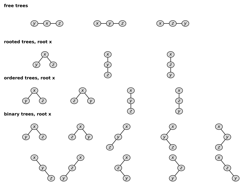
(i) Free trees. A tree on 3 vertices has 2 edges (Theorem B.2), so it is a path, determined by its middle vertex: \(y - x - z\), \(x - y - z\), \(x - z - y\).
(ii) Rooted trees with root \(x\). Rooting each free tree at \(x\) gives: \(x\) with children \(y\) and \(z\); the chain \(x \to y \to z\); the chain \(x \to z \to y\).
(iii) Ordered trees with root \(x\). The rooted tree in which \(x\) has two children splits into two ordered trees (children in order \(y, z\) or \(z, y\)); each chain has only one ordering, giving \(2 + 1 + 1 = 4\).
(iv) Binary trees with root \(x\). When \(x\) has two children, either \(y\) or \(z\) is the left child (2 trees). In each of the two chains, each of the 2 edges independently goes to a left or a right child, giving \(2 \cdot 2^2 = 8\) trees. Total \(2 + 8 = 10\).
Let \(G = (V, E)\) be a directed acyclic graph containing a vertex \(v_0 \in V\) from which every vertex \(v \in V\) is reached by exactly one path. Prove that the undirected version of \(G\) is a tree.
Every vertex other than \(v_0\) has in-degree exactly 1 and \(v_0\) has in-degree 0, so the undirected version \(G^{\prime}\) is connected with \(|V| - 1\) edges, hence a tree by Theorem B.2 ((4) \(\Rightarrow\) (1)).
In-degree of \(v_0\): if \((u, v_0) \in E\), then the path from \(v_0\) to \(u\) followed by the edge \((u, v_0)\) is a cycle, contradicting acyclicity.
In-degree of \(v \ne v_0\): the unique path from \(v_0\) to \(v\) has positive length, and its last edge enters \(v\), so the in-degree is at least 1. If \((u, v), (w, v) \in E\) with \(u \ne w\), then
\begin{equation*} \langle v_0 \leadsto u, v \rangle \quad\text{and}\quad \langle v_0 \leadsto w, v \rangle \end{equation*}
are two paths from \(v_0\) to \(v\) with different last edges, contradicting uniqueness. Summing in-degrees,
\begin{equation*} |E| = \sum_{v \in V} \text{in-degree}(v) = 0 + (|V| - 1) \cdot 1 = |V| - 1 . \end{equation*}
A dag has no self-loops and never contains both \((u, v)\) and \((v, u)\) (that would be a cycle), so distinct edges of \(E\) give distinct edges of \(G^{\prime}\) and \(|E^{\prime}| = |E| = |V| - 1\). Finally \(G^{\prime}\) is connected: any two vertices \(u, v\) are joined through \(v_0\) by the paths \(v_0 \leadsto u\) and \(v_0 \leadsto v\) with directions removed.
Prove by induction that in every nonempty binary tree the number of nodes of degree 2 is one less than the number of leaves. Deduce that a full binary tree has one fewer internal node than it has leaves.
Write \(\ell(T)\) for the number of leaves and \(d_2(T)\) for the number of degree-2 nodes; we prove \(\ell(T) = d_2(T) + 1\) by induction on the number \(n\) of nodes.
For \(n = 1\) the root is a leaf: \(\ell = 1\), \(d_2 = 0\). For \(n > 1\) let the root \(r\) have left and right subtrees \(T_L, T_R\), not both empty; each has fewer than \(n\) nodes, the leaves of \(T\) are the leaves of \(T_L\) and \(T_R\), and the degree-2 nodes of \(T\) are those of \(T_L\) and \(T_R\) plus possibly \(r\).
(i) Both subtrees nonempty (\(r\) has degree 2):
\begin{equation*} \ell(T) = \ell(T_L) + \ell(T_R) = (d_2(T_L) + 1) + (d_2(T_R) + 1) = d_2(T) + 1 . \end{equation*}
(ii) Exactly one subtree \(T^{\prime}\) nonempty (\(r\) has degree 1, not a leaf):
\begin{equation*} \ell(T) = \ell(T^{\prime}) = d_2(T^{\prime}) + 1 = d_2(T) + 1 . \end{equation*}
In a full binary tree every internal node has degree exactly 2, so the number of internal nodes is \(d_2(T) = \ell(T) - 1\).
Prove by induction that a nonempty binary tree with \(n\) nodes has height at least \(\lfloor \lg n \rfloor\).
Induct on \(n\); for \(n = 1\) the height is \(0 = \lfloor \lg 1 \rfloor\).
For \(n \ge 2\) the root’s two subtrees have \(a + b = n - 1\) nodes, so the larger one has \(m \ge \lceil (n-1)/2 \rceil = \lfloor n/2 \rfloor \ge 1\) nodes and, by the induction hypothesis, height at least \(\lfloor \lg m \rfloor\). Since the tree’s height is at least 1 plus the height of each nonempty subtree, and \(\lfloor \lg \cdot \rfloor\) is nondecreasing,
\begin{equation*} h(T) \ge 1 + \lfloor \lg m \rfloor \ge 1 + \lfloor \lg \lfloor n/2 \rfloor \rfloor = \lfloor \lg n \rfloor , \end{equation*}
where the last equality holds because \(2^k \le n < 2^{k+1}\) implies \(2^{k-1} \le \lfloor n/2 \rfloor \le n/2 < 2^k\).
For a full binary tree, the internal path length is the sum of the depths of its internal nodes, and the external path length is the sum of the depths of its leaves. Suppose a full binary tree has \(n\) internal nodes, internal path length \(i\) and external path length \(e\). Prove that \(e = i + 2n\).
Induct on \(n\); for \(n = 0\) the tree is a single leaf at depth 0, so \(e = i = 0\).
For \(n \ge 1\) let \(x\) be an internal node of maximum depth \(d\). Its two children are deeper than every internal node, so both are leaves. Deleting them yields a full binary tree \(T^{\prime}\) with \(n - 1\) internal nodes in which \(x\) is a leaf; its path lengths satisfy \(i = i^{\prime} + d\) (the internal node \(x\) is lost) and \(e = e^{\prime} - d + 2(d+1)\) (leaf \(x\) is replaced by two leaves at depth \(d + 1\)). By the induction hypothesis \(e^{\prime} = i^{\prime} + 2(n-1)\), so
\begin{equation*} e = e^{\prime} + d + 2 = i^{\prime} + 2(n-1) + d + 2 = (i^{\prime} + d) + 2n = i + 2n . \end{equation*}
In a binary tree \(T\) with leaf set \(L\), give each leaf \(x\) of depth \(d\) the weight \(w(x) = 2^{-d}\). Prove the Kraft inequality
\begin{equation*} \sum_{x \in L} w(x) \le 1 . \end{equation*}
Write \(K(T) = \sum_{x \in L} 2^{-\text{depth}(x)}\); we prove \(K(T) \le 1\) by induction on the number of nodes.
If \(T\) is empty, \(K(T) = 0\); if \(T\) is a single node, its root is a leaf of depth 0 and \(K(T) = 1\). Otherwise the root has subtrees \(T_L, T_R\) (possibly one empty), the root is not a leaf, and every leaf of \(T\) is a leaf of \(T_L\) or \(T_R\) whose depth in \(T\) is one more than its depth in the subtree. Hence, by the induction hypothesis applied to the smaller trees \(T_L, T_R\),
\begin{equation*} K(T) = \tfrac12 K(T_L) + \tfrac12 K(T_R) \le \tfrac12 + \tfrac12 = 1 . \end{equation*}
Let \(L \ge 2\). Prove that any binary tree with \(L\) leaves has a subtree (a node together with all of its descendants) whose number of leaves lies in the closed interval \([L/3,\, 2L/3]\).
Walk down from the root, always stepping to the child whose subtree has more leaves, and stop at the first node whose subtree has at most \(2L/3\) leaves; that subtree works.
Write \(\ell(x)\) for the number of leaves in the subtree rooted at \(x\). If \(x\) is not a leaf, its subtree’s leaves are exactly the leaves of its (one or two) children’s subtrees, so
\begin{equation*} \ell(x) = \sum_{c \text{ a child of } x} \ell( c), \qquad\text{hence}\qquad \max_{c} \ell( c) \ge \tfrac{1}{2}\,\ell(x), \end{equation*}
because \(x\) has at most two children.
Start at the root \(r\), where \(\ell( r) = L > 2L/3\) since \(L > 0\). While the current node \(x\) has \(\ell(x) > 2L/3\), move to a child \(c\) of \(x\) maximizing \(\ell( c)\). This is always possible: \(\ell(x) > 2L/3 \ge 4/3 > 1\) (using \(L \ge 2\)), so \(x\) is not a leaf. Every step increases the depth, so the walk stops at some node \(y \ne r\) with \(\ell(y) \le 2L/3\), whose parent \(x\) satisfies \(\ell(x) > 2L/3\) and \(y\) was chosen to maximize \(\ell\) among the children of \(x\). Therefore
\begin{equation*} \frac{L}{3} < \frac{1}{2}\,\ell(x) \le \ell(y) \le \frac{2L}{3}, \end{equation*}
so the subtree rooted at \(y\) has between \(L/3\) and \(2L/3\) leaves. \(\blacksquare\)
Problems for Appendix B
Graph coloring: for an undirected graph \(G=(V,E)\), a \(k\)-coloring is a map \(c : V \to \{0,1,\ldots,k-1\}\) with \(c(u) \ne c(v)\) for every edge \((u,v) \in E\); that is, the \(k\) numbers are colors and the endpoints of each edge get different colors.
(a) Prove that every tree is 2-colorable.
(b) Prove that the following three conditions are equivalent: (1) \(G\) is bipartite; (2) \(G\) is 2-colorable; (3) \(G\) contains no cycle of odd length.
(c) If \(d\) is the largest degree of a vertex of \(G\), prove that \(G\) can be colored with \(d+1\) colors.
(d) Prove that if \(G\) has \(O(|V|)\) edges, then \(G\) can be colored with \(O(\sqrt{|V|})\) colors.
(a) Root the tree at any vertex \(r\) and color each vertex by the parity of its depth, \(c(v) = \operatorname{depth}(v) \bmod 2\). Every edge of a rooted tree joins a node to its parent, whose depths differ by exactly \(1\), so its endpoints get different colors.
(b) (1) \(\Rightarrow\) (2): if \(V = V_1 \cup V_2\) with every edge between \(V_1\) and \(V_2\), put \(c = 0\) on \(V_1\) and \(c = 1\) on \(V_2\).
(2) \(\Rightarrow\) (3): along a cycle \(\langle v_0, v_1, \ldots, v_k = v_0 \rangle\) the colors alternate, so \(c(v_i) \equiv c(v_0) + i \pmod 2\); at \(i = k\) this gives \(k \equiv 0 \pmod 2\).
(3) \(\Rightarrow\) (1): first, a closed walk of odd length contains an odd cycle. Induct on the length \(\ell\). There are no self-loops, so \(\ell \ge 3\). If no vertex repeats apart from the shared endpoint, the walk is itself a cycle. Otherwise, splitting it at a repeated vertex gives two shorter closed walks whose lengths add up to \(\ell\), so one of them has odd length, and induction applies to it. Now, in each connected component pick a vertex \(r\), and let \(V_1\) be the vertices whose distance \(\delta(r,v)\) from \(r\) is even and \(V_2\) the rest. If some edge \((u,v)\) had \(\delta(r,u) \equiv \delta(r,v) \pmod 2\), then a shortest path from \(r\) to \(u\), the edge \((u,v)\), and a shortest path from \(v\) back to \(r\) would form a closed walk of odd length
\begin{equation*} \delta(r,u) + 1 + \delta(r,v), \end{equation*}
which contains an odd cycle, contradicting (3). So every edge goes between \(V_1\) and \(V_2\).
(c) Color the vertices greedily in any order, giving each vertex the smallest color in \(\{0,1,\ldots,d\}\) not already used by one of its colored neighbors. A vertex has at most \(d\) neighbors, so they block at most \(d\) of the \(d+1\) colors and one is always free. Each edge \((u,v)\) is checked when the later of \(u,v\) is colored, so the coloring is proper.
(d) Let \(n = |V|\) and \(|E| \le an\) for a constant \(a\). Let \(H = \{v : \deg(v) \ge \sqrt n\}\) and \(L = V - H\). By the handshaking lemma (Exercise B.4-1),
\begin{equation*} |H|\sqrt n \le \sum_{v \in V} \deg(v) = 2|E| \le 2an, \qquad\text{so}\qquad |H| \le 2a\sqrt n . \end{equation*}
Give each vertex of \(H\) its own color. The induced subgraph \(G[L]\) has maximum degree below \(\sqrt n\), so by (c) it can be colored with at most \(\sqrt n + 1\) further colors, taken from a separate palette. Edges inside \(H\) have distinct colors at their ends, edges between \(H\) and \(L\) use disjoint palettes, and edges inside \(L\) are handled by (c). In total
\begin{equation*} |H| + \sqrt n + 1 \le (2a+1)\sqrt n + 1 = O(\sqrt{|V|}) \end{equation*}
colors are used.
Friendly graphs: restate each claim below as a theorem about undirected graphs and prove it. Friendship is taken to be symmetric and not reflexive.
(a) In any group of two or more people, some two people have the same number of friends within the group.
(b) In any group of six people there are three who are all friends with one another, or three who are all strangers to one another.
(c) Any group of people can be split into two subgroups so that, for each person, at least half of that person’s friends lie in the subgroup the person does not belong to.
(d) If each person in a group is friends with at least half of the people in the group, then the group can be seated around a table so that every person sits between two friends.
(a) Theorem: every simple undirected graph \(G=(V,E)\) (people as vertices, friendships as edges) with \(n = |V| \ge 2\) vertices has two vertices of equal degree. Each degree lies in \(\{0,1,\ldots,n-1\}\). The values \(0\) and \(n-1\) cannot both occur, since a vertex of degree \(n-1\) is adjacent to every other vertex, so no vertex is isolated. The \(n\) degrees therefore take at most \(n-1\) values, and by the pigeonhole principle two of them are equal.
(b) Theorem: every graph on \(6\) vertices contains a triangle or an independent set of size \(3\) (in other words, \(G\) or its complement contains a \(K_3\)). Fix a vertex \(v\). Of the other \(5\) vertices, at least \(3\) are neighbors of \(v\) or at least \(3\) are non-neighbors. (i) Say \(a,b,c\) are neighbors of \(v\). If some pair of them is adjacent, that pair together with \(v\) is a triangle; otherwise \(\{a,b,c\}\) is independent. (ii) Say \(a,b,c\) are non-neighbors of \(v\). If some pair of them is non-adjacent, that pair together with \(v\) is independent; otherwise \(\{a,b,c\}\) is a triangle.
(c) Theorem: every graph has a partition \(V = S \cup (V - S)\) in which each vertex \(v\) has at least \(\deg(v)/2\) neighbors on the side not containing \(v\). Choose \(S\) so that the number of edges crossing the cut \((S, V-S)\) is as large as possible; there are finitely many choices, so a maximizer exists. Suppose some \(v\) has \(s\) neighbors on its own side and \(t\) on the other, with \(t < \deg(v)/2\), that is, \(s > t\). Moving \(v\) to the other side turns those \(s\) edges into crossing edges and the \(t\) edges into non-crossing ones, so the cut grows by \(s - t > 0\). This contradicts maximality. (If both subgroups must be non-empty and \(n \ge 2\): a maximum cut with an empty side crosses \(0\) edges, so \(E = \emptyset\) and any split into two non-empty parts works.)
(d) Theorem (Dirac): if \(n \ge 3\) and \(\deg(v) \ge n/2\) for every \(v\), then \(G\) has a Hamiltonian cycle, that is, a cycle through all \(n\) vertices. (For \(n = 2\) the hypothesis makes the two people friends, and each is seated between the other on both sides; for \(n = 1\) the hypothesis cannot hold, because there are no self-loops.)
\(G\) is connected: two non-adjacent vertices \(u,w\) have \(\deg(u) + \deg(w) \ge n\) neighbors counted with multiplicity, all among the other \(n-2\) vertices, so they share a neighbor. Let \(P = \langle v_0, v_1, \ldots, v_k \rangle\) be a longest simple path. By maximality every neighbor of \(v_0\) and every neighbor of \(v_k\) lies on \(P\). Define
\begin{equation*} \begin{aligned} A &= \{\, i \in \{1,\ldots,k\} : (v_0, v_i) \in E \,\},\\ B &= \{\, i \in \{1,\ldots,k\} : (v_{i-1}, v_k) \in E \,\}. \end{aligned} \end{equation*}
Then \(|A| = \deg(v_0) \ge n/2\) and \(|B| = \deg(v_k) \ge n/2\), so \(|A| + |B| \ge n > k\), because \(k \le n-1\). Hence there is some \(i \in A \cap B\), and
\begin{equation*} C = \langle v_0, v_i, v_{i+1}, \ldots, v_k, v_{i-1}, v_{i-2}, \ldots, v_1, v_0 \rangle \end{equation*}
is a cycle through all \(k+1\) vertices of \(P\). When \(i = 1\) this reads \(v_0, v_1, \ldots, v_k, v_0\). It is a genuine cycle because \(k \ge |A| \ge n/2 > 1\), so it has \(k+1 \ge 3\) vertices. If \(k+1 < n\), connectivity gives a vertex \(w \notin C\) adjacent to some \(v_j \in C\). Starting at \(w\), stepping to \(v_j\), and then walking once around \(C\) gives a simple path with \(k+1\) edges, which contradicts the maximality of \(P\). So \(k+1 = n\) and \(C\) is Hamiltonian. Seating the people in the order of \(C\) places everyone between two friends.
Bisecting trees: divide-and-conquer algorithms on graphs often need to split the vertex set into two parts of nearly equal size. Here we split a tree by deleting a few edges, subject to the rule that any two vertices lying in the same component of the remaining forest must be placed in the same part.
(a) Prove that for any binary tree with \(n\) vertices, deleting a single edge suffices to partition the vertices into sets \(A\) and \(B\) with \(|A| \le 3n/4\) and \(|B| \le 3n/4\).
(b) Prove that the constant \(3/4\) in part (a) cannot be improved in the worst case: exhibit a simple binary tree for which the most balanced partition obtainable by deleting one edge has \(|A| = 3n/4\).
(c) Prove that by deleting at most \(O(\lg n)\) edges one can partition the vertices of any \(n\)-vertex binary tree into sets \(A\) and \(B\) with \(|A| = \lfloor n/2 \rfloor\) and \(|B| = \lceil n/2 \rceil\).
(a) Delete the edge above a vertex \(v\) of minimum \(s(v)\) among those with \(s(v) > n/4\), where \(s(v)\) is the size of the subtree rooted at \(v\) and \(n \ge 2\); this splits the tree into two rooted binary trees of sizes \(s(v)\) and \(n - s(v)\). If \(n \le 4\), any edge works, since both parts have sizes between \(1\) and \(n - 1 \le 3n/4\). Let \(n \ge 5\). The root qualifies (\(s = n > n/4\)), so \(v\) exists; each child \(c\) of \(v\) has \(s( c) \le n/4\) by minimality, and \(v\) has at most two children, so
\begin{equation*} \frac{n}{4} < s(v) \le 1 + 2 \cdot \frac{n}{4} = \frac{n}{2} + 1 \le \frac{3n}{4} \qquad (n \ge 4). \end{equation*}
In particular \(s(v) < n\), so \(v\) is not the root and the edge to its parent exists. Put \(B\) = subtree of \(v\) and \(A\) = the rest: \(|B| = s(v) \le 3n/4\) and \(|A| = n - s(v) < 3n/4\).
(b) Take \(n = 4\): a root \(r\) with a single child \(a\), and \(a\) with two children \(b\) and \(c\). The three edges \(ra\), \(ab\), \(ac\) each cut off a single vertex (\(r\), \(b\), \(c\) respectively), so every one-edge partition has part sizes \(1\) and \(3\); the most balanced has \(|A| = 3 = 3n/4\).
(c) Repeatedly apply part (a) to the piece still to be divided; this uses at most \(\log_{4/3}(n/2) + 1 = O(\lg n)\) deletions. Let \(k = \lfloor n/2 \rfloor\). Maintain sets \(A_0, B_0\) of already-assigned vertices, a current rooted binary tree \(T\) (a component of the current forest) of size \(m\), and a target \(t\), with the invariant
\begin{equation*} V = A_0 \cup B_0 \cup V(T) \ \text{(disjoint)}, \qquad |A_0| + t = k, \qquad 0 \le t \le m, \end{equation*}
and every component of the forest other than \(T\) lies wholly in \(A_0\) or wholly in \(B_0\). Initially \(A_0 = B_0 = \emptyset\), \(T\) is the whole tree, \(t = k \le n\).
While \(0 < t < m\) (so \(m \ge 2\)), delete one edge of \(T\) by part (a), splitting it into trees \(P, Q\) with \(|P|, |Q| \le 3m/4\). (i) If \(t \le |P|\): move \(Q\) into \(B_0\) and continue with \(T := P\), target \(t\). (ii) If \(t > |P|\): move \(P\) into \(A_0\) and continue with \(T := Q\), target \(t - |P|\), which lies in \((0, |Q|]\) because \(t \le m = |P| + |Q|\). In both cases \(P\) or \(Q\) becomes an untouched component assigned wholesale, so the invariant is preserved.
When \(t = 0\) put \(T\) into \(B_0\); when \(t = m\) put \(T\) into \(A_0\). Now every component lies in one part, and \(|A| = |A_0| + t = k = \lfloor n/2 \rfloor\), \(|B| = n - k = \lceil n/2 \rceil\).
After \(i\) deletions the current tree has \(m \le (3/4)^i n\), and a further deletion happens only if \(m \ge 2\). Hence if \(d\) deletions occur in total, \(2 \le (3/4)^{d-1} n\), so
\begin{equation*} d \le \log_{4/3}\frac{n}{2} + 1 = O(\lg n). \end{equation*}
Appendix C: Counting and Probability
C.1 Counting
Count the \(k\)-substrings of an \(n\)-string, treating equal \(k\)-substrings that sit at different positions as distinct. Then count all substrings of an \(n\)-string.
An \(n\)-string has \(n-k+1\) \(k\)-substrings (for \(1 \le k \le n\)), and \(n(n+1)/2\) nonempty substrings in total.
A \(k\)-substring is a block of \(k\) consecutive positions \(s_i s_{i+1} \cdots s_{i+k-1}\), determined by its starting index \(i\), and \(i\) ranges over \(1 \le i \le n-k+1\). Summing over the lengths,
\begin{equation*} \sum_{k=1}^{n} (n-k+1) = \sum_{j=1}^{n} j = \frac{n(n+1)}{2} \end{equation*}
by the arithmetic series (A.1).
A boolean function with \(n\) inputs and \(m\) outputs is a function \(\{\text{TRUE}, \text{FALSE}\}^n \to \{\text{TRUE}, \text{FALSE}\}^m\). How many boolean functions with \(n\) inputs and \(1\) output exist? How many with \(n\) inputs and \(m\) outputs?
There are \(2^{2^n}\) functions with one output and \(2^{m 2^n}\) with \(m\) outputs.
The domain \(\{\text{TRUE}, \text{FALSE}\}^n\) has \(2^n\) elements and the codomain \(\{\text{TRUE}, \text{FALSE}\}^m\) has \(2^m\). A function picks one codomain element for each domain element, independently, so the number of functions is
\begin{equation*} \left(2^m\right)^{2^n} = 2^{m 2^n}, \end{equation*}
and \(m=1\) gives \(2^{2^n}\).
Count the ways \(n\) professors can be seated around a circular conference table, where two seatings are identified if a rotation carries one to the other.
There are \((n-1)!\) seatings.
The \(n\) rotations of a seating are all distinct seatings of the table (the professors are distinct people, so a nontrivial rotation moves professor \(1\) to a different seat), so each rotation class of the \(n!\) linear seatings has exactly \(n\) elements, and there are \(n!/n = (n-1)!\) classes.
Method (2): rotate professor \(1\) into a fixed seat, and the remaining \(n-1\) professors fill the other seats in \((n-1)!\) ways (by (C.1) for an \((n-1)\)-set with \(k=n-1\)).
Count the ways to choose three distinct numbers from \(\{1, 2, \ldots, 99\}\) whose sum is even.
There are \(78449\) ways.
The set has \(50\) odd and \(49\) even numbers. A sum of three integers is even exactly when the number of odd summands is even, i.e. \(0\) or \(2\):
\begin{equation*} \begin{aligned} \binom{49}{3} + \binom{50}{2}\binom{49}{1} &= 18424 + 1225 \cdot 49 \\ &= 18424 + 60025 = 78449 . \end{aligned} \end{equation*}
Prove that
\begin{equation*} \binom{n}{k} = \frac{n}{k}\binom{n-1}{k-1} \qquad (\text{C.8}) \end{equation*}
whenever \(0 < k \le n\).
Both sides equal \(n!/(k!\,(n-k)!)\). Since \(0 \le k-1 \le n-1\), (C.2) applies to \(\binom{n-1}{k-1}\), and \((n-1)-(k-1) = n-k\):
\begin{equation*} \frac{n}{k}\binom{n-1}{k-1} = \frac{n}{k}\cdot\frac{(n-1)!}{(k-1)!\,(n-k)!} = \frac{n!}{k!\,(n-k)!} = \binom{n}{k}, \end{equation*}
using \(n\,(n-1)! = n!\) and \(k\,(k-1)! = k!\) (valid as \(k \ge 1\)).
Prove that
\begin{equation*} \binom{n}{k} = \frac{n}{n-k}\binom{n-1}{k} \end{equation*}
whenever \(0 \le k < n\).
Both sides equal \(n!/(k!\,(n-k)!)\). Since \(0 \le k \le n-1\), (C.2) applies to \(\binom{n-1}{k}\), and \((n-1)-k = n-k-1 \ge 0\):
\begin{equation*} \frac{n}{n-k}\binom{n-1}{k} = \frac{n}{n-k}\cdot\frac{(n-1)!}{k!\,(n-k-1)!} = \frac{n!}{k!\,(n-k)!} = \binom{n}{k}, \end{equation*}
using \(n\,(n-1)! = n!\) and \((n-k)\,(n-k-1)! = (n-k)!\) (valid as \(n-k \ge 1\)).
Method (2): apply (C.3), then C.1-5 with \(n-k\) in place of \(k\) (allowed since \(0 < n-k \le n\)), then (C.3) again:
\begin{equation*} \begin{aligned} \binom{n}{k} = \binom{n}{n-k} &= \frac{n}{n-k}\binom{n-1}{n-k-1} \\ &= \frac{n}{n-k}\binom{n-1}{k}. \end{aligned} \end{equation*}
One way to pick \(k\) of \(n\) objects is to single out one object and split according to whether it is picked. Using this idea, prove Pascal’s rule
\begin{equation*} \binom{n}{k} = \binom{n-1}{k} + \binom{n-1}{k-1}. \end{equation*}
Fix \(n \ge 1\), an \(n\)-set \(S\), and a distinguished element \(x \in S\); the \(k\)-subsets of \(S\) split into two disjoint classes.
(i) Those not containing \(x\): these are exactly the \(k\)-subsets of the \((n-1)\)-set \(S - \{x\}\), so there are \(\binom{n-1}{k}\) of them.
(ii) Those containing \(x\): \(T \mapsto T - \{x\}\) is a bijection onto the \((k-1)\)-subsets of \(S - \{x\}\) (inverse \(U \mapsto U \cup \{x\}\)), so there are \(\binom{n-1}{k-1}\) of them.
Adding the two counts gives \(\binom{n}{k} = \binom{n-1}{k} + \binom{n-1}{k-1}\). This holds for all \(0 \le k \le n\) with the convention that \(\binom{m}{j} = 0\) when \(j < 0\) or \(j > m\) (at \(k = 0\) class (ii) is empty, at \(k = n\) class (i) is empty).
Use the result of Exercise C.1-7 to tabulate the binomial coefficients \(\binom{n}{k}\) for \(n = 0, 1, \ldots, 6\) and \(0 \le k \le n\), arranged with \(\binom{0}{0}\) on the top row, \(\binom{1}{0}\) and \(\binom{1}{1}\) on the next row, and so on. This table is known as Pascal’s triangle.
Each row starts and ends with \(\binom{n}{0} = \binom{n}{n} = 1\), and every interior entry is the sum of the two entries above it, \(\binom{n}{k} = \binom{n-1}{k} + \binom{n-1}{k-1}\) by Exercise C.1-7:
| \(n\) | \(k=0\) | \(k=1\) | \(k=2\) | \(k=3\) | \(k=4\) | \(k=5\) | \(k=6\) |
|---|---|---|---|---|---|---|---|
| 0 | 1 | ||||||
| 1 | 1 | 1 | |||||
| 2 | 1 | 2 | 1 | ||||
| 3 | 1 | 3 | 3 | 1 | |||
| 4 | 1 | 4 | 6 | 4 | 1 | ||
| 5 | 1 | 5 | 10 | 10 | 5 | 1 | |
| 6 | 1 | 6 | 15 | 20 | 15 | 6 | 1 |
Prove that
\begin{equation*} \sum_{i=1}^{n} i = \binom{n+1}{2}. \end{equation*}
Count the 2-subsets \(\{i, j\}\), \(i < j\), of \(\{1, 2, \ldots, n+1\}\) by their larger element \(j\): for each \(j \in \{2, \ldots, n+1\}\) there are exactly \(j - 1\) choices of \(i \in \{1, \ldots, j-1\}\), so
\begin{equation*} \binom{n+1}{2} = \sum_{j=2}^{n+1} (j-1) = \sum_{i=1}^{n} i . \end{equation*}
Method (2): induction on \(n\) with Exercise C.1-7. For \(n = 0\) both sides are \(0\) (as \(\binom{1}{2} = 0\)), and
\begin{equation*} \binom{n+1}{2} = \binom{n}{2} + \binom{n}{1} = \sum_{i=1}^{n-1} i + n = \sum_{i=1}^{n} i . \end{equation*}
Show that for all integers \(n \ge 0\) and \(0 \le k \le n\), the value of \(\binom{n}{k}\) is largest when \(k = \lfloor n/2 \rfloor\) or \(k = \lceil n/2 \rceil\).
The sequence \(\binom{n}{0}, \ldots, \binom{n}{n}\) rises strictly up to \(k = \lfloor n/2 \rfloor\), is constant from \(\lfloor n/2 \rfloor\) to \(\lceil n/2 \rceil\), and falls strictly afterwards. Indeed, for \(0 \le k < n\) the formula (C.2) gives
\begin{equation*} \frac{\binom{n}{k+1}}{\binom{n}{k}} = \frac{k!\,(n-k)!}{(k+1)!\,(n-k-1)!} = \frac{n-k}{k+1}, \end{equation*}
which is \(> 1\), \(= 1\) or \(< 1\) according as \(k < (n-1)/2\), \(k = (n-1)/2\) or \(k > (n-1)/2\). Hence:
(i) \(n\) even: the ratio exceeds \(1\) for \(k \le n/2 - 1\) and is below \(1\) for \(k \ge n/2\), so the unique maximum is at \(k = n/2 = \lfloor n/2 \rfloor = \lceil n/2 \rceil\).
(ii) \(n\) odd: the ratio exceeds \(1\) for \(k < (n-1)/2\), equals \(1\) at \(k = (n-1)/2\), and is below \(1\) for \(k > (n-1)/2\), so the maximum value is attained at both \(k = (n-1)/2 = \lfloor n/2 \rfloor\) and \(k = (n+1)/2 = \lceil n/2 \rceil\).
Show that for all integers \(n \ge 0\), \(j \ge 0\), \(k \ge 0\) with \(j + k \le n\),
\begin{equation*} \binom{n}{j+k} \le \binom{n}{j}\binom{n-j}{k}. \qquad \text{(C.9)} \end{equation*}
Give an algebraic proof and also a proof based on a procedure for selecting \(j + k\) of the \(n\) items. Exhibit a case where the inequality is strict.
In fact \(\binom{n}{j}\binom{n-j}{k} = \binom{n}{j+k}\binom{j+k}{j}\), and \(\binom{j+k}{j} \ge 1\).
Algebraic proof. By (C.2),
\begin{equation*} \begin{aligned} \binom{n}{j}\binom{n-j}{k} &= \frac{n!}{j!\,(n-j)!}\cdot\frac{(n-j)!}{k!\,(n-j-k)!} = \frac{n!}{(j+k)!\,(n-j-k)!}\cdot\frac{(j+k)!}{j!\,k!} \\ &= \binom{n}{j+k}\binom{j+k}{j} \ \ge\ \binom{n}{j+k}. \end{aligned} \end{equation*}
Combinatorial proof. Choose \(j + k\) items in two rounds: first a \(j\)-subset \(J\) of the \(n\) items, then a \(k\)-subset \(K\) of the remaining \(n - j\). There are \(\binom{n}{j}\binom{n-j}{k}\) pairs \((J, K)\), and each yields the \((j+k)\)-subset \(J \cup K\). Every \((j+k)\)-subset \(T\) arises this way (take any \(j\)-subset \(J \subseteq T\) and \(K = T - J\)), so the number of \((j+k)\)-subsets, \(\binom{n}{j+k}\), is at most the number of pairs.
Strict example: \(n = 2\), \(j = k = 1\) gives \(\binom{2}{2} = 1 < 2 = \binom{2}{1}\binom{1}{1}\); the subset \(\{a, b\}\) arises from both \((J,K) = (\{a\},\{b\})\) and \((\{b\},\{a\})\).
Prove inequality (C.6),
\begin{equation*} \binom{n}{k} \le \frac{n^n}{k^k (n-k)^{n-k}} \qquad (\text{with } 0^0 = 1), \end{equation*}
by induction over the integers \(k\) with \(0 \le k \le n/2\), and then use the symmetry (C.3) to extend it to every integer \(k\) with \(0 \le k \le n\).
Fix \(n \ge 0\) and induct on \(k\). For \(k = 0\) both sides equal \(1\), since \(n^n / (0^0 n^n) = 1\) (also when \(n = 0\)).
Suppose (C.6) holds for some \(k\) with \(k + 1 \le n/2\), and put \(m = n - k - 1\), so \(m \ge k + 1\). Using \(\binom{n}{k+1} = \binom{n}{k}\frac{n-k}{k+1}\) (from (C.2)) and the hypothesis,
\begin{equation*} \binom{n}{k+1} \le \frac{n^n}{k^k (n-k)^{n-k}}\cdot\frac{n-k}{k+1} = \frac{n^n}{(k+1)\,k^k\,(m+1)^{m}} , \end{equation*}
and this is at most the desired bound \(n^n / \bigl((k+1)^{k+1} m^{m}\bigr)\) exactly when
\begin{equation*} (k+1)^k\, m^m \le k^k\, (m+1)^m . \qquad (*) \end{equation*}
(i) \(k = 0\): \((*)\) reads \(m^m \le (m+1)^m\), true.
(ii) \(k \ge 1\): \((*)\) is \(a_k \le a_m\) for \(a_t = (1 + 1/t)^t\), which holds because \(m > k\) and \(a_t\) is nondecreasing in the integer \(t \ge 1\): by the AM-GM inequality applied to \(t\) copies of \(1 + 1/t\) and one \(1\),
\begin{equation*} a_t = \Bigl(1 + \frac1t\Bigr)^t \cdot 1 \le \Bigl(\frac{t(1 + 1/t) + 1}{t+1}\Bigr)^{t+1} = \Bigl(1 + \frac{1}{t+1}\Bigr)^{t+1} = a_{t+1}. \end{equation*}
This completes the induction, so (C.6) holds for \(0 \le k \le n/2\).
For \(n/2 < k \le n\) we have \(0 \le n - k < n/2\), so by (C.3) and the case just proved (applied to \(n - k\)),
\begin{equation*} \binom{n}{k} = \binom{n}{n-k} \le \frac{n^n}{(n-k)^{n-k}\,\bigl(n-(n-k)\bigr)^{n-(n-k)}} = \frac{n^n}{k^k (n-k)^{n-k}} . \end{equation*}
Using Stirling’s approximation, prove equation (C.10):
\begin{equation*} \binom{2n}{n} = \frac{2^{2n}}{\sqrt{\pi n}}\bigl(1 + O(1/n)\bigr). \end{equation*}
Substitute Stirling’s approximation (3.18), \(m! = \sqrt{2\pi m}\,(m/e)^m(1+\Theta(1/m))\), for \((2n)!\) and \(n!\). Write the error factors as \(1+a_n\) for \((2n)!\) and \(1+b_n\) for \(n!\), where \(|a_n|,|b_n| \le c/n\) for some constant \(c\) and all \(n \ge 1\). Then
\begin{equation*} \begin{aligned} \binom{2n}{n} = \frac{(2n)!}{(n!)^2} &= \frac{\sqrt{4\pi n}\,(2n/e)^{2n}(1+a_n)}{2\pi n\,(n/e)^{2n}(1+b_n)^2} \\ &= \frac{2\sqrt{\pi n}\,2^{2n}}{2\pi n}\cdot\frac{1+a_n}{(1+b_n)^2} = \frac{2^{2n}}{\sqrt{\pi n}}\cdot\frac{1+a_n}{(1+b_n)^2}. \end{aligned} \end{equation*}
It remains to show that the last factor is \(1+O(1/n)\). For \(n \ge 2c\) we have \(|b_n| \le 1/2\), so \((1+b_n)^2 \ge 1/4\) and
\begin{equation*} \left|\frac{1+a_n}{(1+b_n)^2} - 1\right| = \frac{|a_n - 2b_n - b_n^2|}{(1+b_n)^2} \le 4\left(\frac{c}{n} + \frac{2c}{n} + \frac{c^2}{n^2}\right) \le \frac{12c + 4c^2}{n}. \end{equation*}
Hence \(\frac{1+a_n}{(1+b_n)^2} = 1 + O(1/n)\), and (C.10) follows. \(\blacksquare\)
Differentiate the entropy function \(H(\lambda) = -\lambda\lg\lambda - (1-\lambda)\lg(1-\lambda)\) of (C.7) to show that its maximum is attained at \(\lambda = 1/2\). What is \(H(1/2)\)?
\(H\) is maximized at \(\lambda = 1/2\), where \(H(1/2) = 1\). For \(0 < \lambda < 1\), using \(\frac{d}{d\lambda}\lg\lambda = \frac{1}{\lambda\ln 2}\),
\begin{equation*} H^{\prime}(\lambda) = -\lg\lambda - \frac{1}{\ln 2} + \lg(1-\lambda) + \frac{1}{\ln 2} = \lg\frac{1-\lambda}{\lambda}. \end{equation*}
So \(H^{\prime}(\lambda) = 0 \iff \lambda = 1/2\), with \(H^{\prime} > 0\) on \((0,1/2)\) and \(H^{\prime} < 0\) on \((1/2,1)\): \(H\) strictly increases up to \(1/2\) and strictly decreases after it. As \(H\) is continuous on \([0,1]\) (\(\lambda\lg\lambda \to 0\) as \(\lambda \to 0^+\), matching \(0\lg 0 = 0\)), \(\lambda = 1/2\) is the global maximum, and
\begin{equation*} H(1/2) = -\tfrac12\lg\tfrac12 - \tfrac12\lg\tfrac12 = -\lg\tfrac12 = 1. \end{equation*}
Prove that every integer \(n \ge 0\) satisfies equation (C.11):
\begin{equation*} \sum_{k=0}^{n} \binom{n}{k} k = n2^{n-1}. \end{equation*}
Use the absorption identity (C.8), \(k\binom{n}{k} = n\binom{n-1}{k-1}\) for \(0 < k \le n\), and then the special case \(2^m = \sum_{j=0}^{m}\binom{m}{j}\) of the binomial expansion (C.4). When \(n = 0\), both sides equal \(0\). When \(n \ge 1\), the \(k = 0\) term is \(0\), so
\begin{equation*} \begin{aligned} \sum_{k=0}^{n}\binom{n}{k}k &= \sum_{k=1}^{n} n\binom{n-1}{k-1} = n\sum_{j=0}^{n-1}\binom{n-1}{j} = n2^{n-1}. \qquad \blacksquare \end{aligned} \end{equation*}
C.2 Probability
Professor Rosencrantz tosses a fair coin one time, and Professor Guildenstern tosses a fair coin two times. Find the probability that Rosencrantz gets strictly more heads than Guildenstern.
The probability is \(1/8\). Rosencrantz has at most one head, so he wins exactly when he gets a head and Guildenstern gets none; the three tosses are independent, so
\begin{equation*} \Pr\{\text{R wins}\} = \Pr\{\text{R: H}\}\cdot\Pr\{\text{G: TT}\} = \frac12\cdot\frac14 = \frac18 . \end{equation*}
Prove Boole’s inequality: for every finite or countably infinite sequence of events \(A_1, A_2, \ldots\),
\begin{equation*} \Pr\{A_1 \cup A_2 \cup \cdots\} \le \Pr\{A_1\} + \Pr\{A_2\} + \cdots . \qquad \text{(C.19)} \end{equation*}
Disjointify: put \(B_1 = A_1\) and \(B_i = A_i - (A_1 \cup \cdots \cup A_{i-1})\) for \(i \ge 2\). Then the \(B_i\) are pairwise mutually exclusive (if \(j < i\) then \(B_i \cap A_j = \emptyset\) and \(B_j \subseteq A_j\)), \(B_i \subseteq A_i\), and \(\bigcup_i B_i = \bigcup_i A_i\) (a point of \(\bigcup_i A_i\) lies in \(B_i\) for the least \(i\) with that point in \(A_i\)). Hence, by axiom 3 (for a finite or countable sequence) and monotonicity (\(B \subseteq A \Rightarrow \Pr\{B\} \le \Pr\{A\}\), noted after the axioms in Section C.2),
\begin{equation*} \Pr\Big\{\bigcup_i A_i\Big\} = \Pr\Big\{\bigcup_i B_i\Big\} = \sum_i \Pr\{B_i\} \le \sum_i \Pr\{A_i\} . \end{equation*}
\(\blacksquare\)
A deck of 10 cards, carrying the distinct numbers \(1, 2, \ldots, 10\), is shuffled thoroughly. Three cards are then drawn from the deck one after another. What is the probability that the three cards come out in increasing order?
The probability is \(1/6\). After a uniform shuffle, every ordered triple of distinct cards is equally likely to be the sequence drawn, so there are \(10\cdot 9\cdot 8 = 720\) equally likely outcomes. Each \(3\)-element set of cards appears in exactly one increasing order, so the favourable outcomes number \(\binom{10}{3} = 120\) and
\begin{equation*} \Pr\{\text{increasing}\} = \frac{\binom{10}{3}}{10\cdot 9\cdot 8} = \frac{120}{720} = \frac{1}{3!} = \frac16 . \end{equation*}
Prove that \(\Pr\{A \mid B\} + \Pr\{\overline{A} \mid B\} = 1\).
Assume \(\Pr\{B\} \neq 0\), as the definition (C.14) of conditional probability requires. The events \(A \cap B\) and \(\overline{A} \cap B\) are mutually exclusive with union \(B\), so by (C.14) and axiom 3,
\begin{equation*} \Pr\{A \mid B\} + \Pr\{\overline{A} \mid B\} = \frac{\Pr\{A \cap B\} + \Pr\{\overline{A} \cap B\}}{\Pr\{B\}} = \frac{\Pr\{B\}}{\Pr\{B\}} = 1 . \qquad \blacksquare \end{equation*}
Prove that for any events \(A_1, A_2, \ldots, A_n\),
\begin{equation*} \begin{aligned} \Pr\{A_1 \cap A_2 \cap \cdots \cap A_n\} &= \Pr\{A_1\}\cdot\Pr\{A_2 \mid A_1\}\cdot\Pr\{A_3 \mid A_1 \cap A_2\} \cdots \\ &\qquad \Pr\{A_n \mid A_1 \cap A_2 \cap \cdots \cap A_{n-1}\} . \end{aligned} \end{equation*}
Write \(C_k = A_1 \cap \cdots \cap A_k\) (so \(C_1 = A_1\)), and assume \(\Pr\{C_{n-1}\} > 0\) so that every conditional probability on the right is defined; since \(C_{n-1} \subseteq C_{k}\) for \(k \le n-1\), also \(\Pr\{C_k\} \ge \Pr\{C_{n-1}\} > 0\). By (C.14), \(\Pr\{A_k \mid C_{k-1}\} = \Pr\{A_k \cap C_{k-1}\}/\Pr\{C_{k-1}\} = \Pr\{C_k\}/\Pr\{C_{k-1}\}\), so the product telescopes:
\begin{equation*} \Pr\{C_1\}\prod_{k=2}^{n} \Pr\{A_k \mid C_{k-1}\} = \Pr\{C_1\}\prod_{k=2}^{n}\frac{\Pr\{C_k\}}{\Pr\{C_{k-1}\}} = \Pr\{C_n\} . \qquad \blacksquare \end{equation*}
Give a procedure whose input is two integers \(a, b\) with \(0 < a < b\) and which, using only fair coin flips, outputs heads with probability \(a/b\) and tails with probability \((b-a)/b\). Bound the expected number of coin flips it uses; the bound should be \(O(1)\). (Hint: write \(a/b\) in binary.)
Flip coins to generate the binary digits \(x_1 x_2 \ldots\) of a uniform random number \(U = 0.x_1x_2\ldots\), generate the binary digits \(c_1 c_2 \ldots\) of \(a/b\) by long division alongside, and stop at the first position \(i\) where \(x_i \ne c_i\): output heads if \(c_i = 1\) (then \(U < a/b\)) and tails if \(c_i = 0\). The expected number of flips is exactly \(2\).
BIASED-COIN(a, b)
1 r = a
2 while TRUE
3 r = 2r // next binary digit c of a/b
4 if r >= b
5 c = 1
6 r = r - b
7 else c = 0
8 x = FAIR-COIN() // 0 or 1, each with probability 1/2
9 if x != c
10 if c == 1
11 return HEADS
12 else return TAILS
Correctness. At the start of the \(k\)th iteration \(0 \le r < b\) (initially \(r = a < b\); and \(0 \le 2r < 2b\), so lines 3-7 leave \(0 \le r < b\)), and after \(k\) iterations the digits satisfy the long-division identity
\begin{equation*} \frac ab = \sum_{i=1}^{k} c_i 2^{-i} + \frac{r_k}{b\,2^{k}}, \qquad 0 \le \frac{r_k}{b\,2^k} < 2^{-k}, \end{equation*}
(check by induction on \(k\)), so \(\sum_{i \ge 1} c_i 2^{-i} = a/b\). The flips are independent and fair, so the procedure returns HEADS in iteration \(i\) exactly when \(x_j = c_j\) for \(j < i\), \(x_i = 0\) and \(c_i = 1\), an event of probability \(c_i 2^{-i}\). These events are mutually exclusive, and the procedure halts with probability \(1\) (it survives \(k\) iterations with probability \(2^{-k}\)), so by axiom 3
\begin{equation*} \begin{aligned} \Pr\{\text{HEADS}\} &= \sum_{i\ge 1} c_i 2^{-i} = \frac ab, \\ \Pr\{\text{TAILS}\} &= 1 - \frac ab = \frac{b-a}{b}. \end{aligned} \end{equation*}
Expected flips. Let \(N\) be the number of flips; \(N \ge i\) iff the first \(i-1\) flips all matched, so \(\Pr\{N \ge i\} = 2^{-(i-1)}\) and by (C.25)
\begin{equation*} \mathrm{E}[N] = \sum_{i \ge 1} \Pr\{N \ge i\} = \sum_{i\ge 1} 2^{-(i-1)} = 2 = O(1), \end{equation*}
independent of \(a\) and \(b\).
Construct, for a given \(n\), a collection of \(n\) events that are pairwise independent, yet such that no subcollection of \(k > 2\) of them is mutually independent.
Use a sample space in which every outcome lies in at most two of the events, with the pairwise intersections weighted so that \(\Pr\{A_i \cap A_j\} = \Pr\{A_i\}\Pr\{A_j\}\). (For \(n \le 2\) there is nothing to prove beyond pairwise independence, so take \(n \ge 3\).)
Let the sample space consist of an outcome \(s_\emptyset\), an outcome \(s_i\) for each \(i \in \{1,\dots,n\}\), and an outcome \(s_{ij}\) for each pair \(1 \le i < j \le n\), with
\begin{equation*} \Pr\{s_i\} = \Pr\{s_{ij}\} = \frac{1}{n^2}, \qquad \Pr\{s_\emptyset\} = \frac{n-1}{2n}, \end{equation*}
and let \(A_i = \{s_i\} \cup \{s_{ij} : j \ne i\}\) (writing \(s_{ij} = s_{ji}\)). This is a probability distribution, since
\begin{equation*} n \cdot \frac{1}{n^2} + \binom{n}{2}\frac{1}{n^2} + \frac{n-1}{2n} = \frac{1}{n} + \frac{n-1}{2n} + \frac{n-1}{2n} = 1 . \end{equation*}
For \(i \ne j\),
\begin{equation*} \begin{aligned} \Pr\{A_i\} &= \frac{1}{n^2} + (n-1)\frac{1}{n^2} = \frac{1}{n}, \\ \Pr\{A_i \cap A_j\} &= \Pr\{s_{ij}\} = \frac{1}{n^2} = \Pr\{A_i\}\Pr\{A_j\}, \end{aligned} \end{equation*}
so the events are pairwise independent. But for any \(k \ge 3\) distinct indices \(i_1,\dots,i_k\), no outcome lies in three of the events, so
\begin{equation*} \Pr\{A_{i_1} \cap \cdots \cap A_{i_k}\} = 0 \ne \frac{1}{n^k} = \Pr\{A_{i_1}\}\cdots\Pr\{A_{i_k}\}, \end{equation*}
and the product condition defining mutual independence fails for the whole subcollection. Hence no \(k > 2\) of the events are mutually independent.
Call events \(A\) and \(B\) conditionally independent given an event \(C\) when
\begin{equation*} \Pr\{A \cap B \mid C\} = \Pr\{A \mid C\} \cdot \Pr\{B \mid C\} . \end{equation*}
Give a simple but nontrivial example of two events that fail to be independent but are conditionally independent given some third event.
Choose one of two coins uniformly at random, a fair coin or a two-headed coin, and flip it twice; let \(A\) = the first flip is heads, \(B\) = the second flip is heads, \(C\) = the fair coin was chosen.
Given \(C\), the two flips are independent fair flips, so
\begin{equation*} \Pr\{A \cap B \mid C\} = \frac14 = \frac12 \cdot \frac12 = \Pr\{A \mid C\}\Pr\{B \mid C\} . \end{equation*}
Unconditionally, conditioning on the coin choice,
\begin{equation*} \begin{aligned} \Pr\{A\} = \Pr\{B\} &= \tfrac12 \cdot \tfrac12 + \tfrac12 \cdot 1 = \tfrac34, \\ \Pr\{A \cap B\} &= \tfrac12 \cdot \tfrac14 + \tfrac12 \cdot 1 = \tfrac58 \ne \tfrac{9}{16} = \Pr\{A\}\Pr\{B\}, \end{aligned} \end{equation*}
so \(A\) and \(B\) are not independent (a first head makes the two-headed coin more likely, which raises the chance of a second head). All of \(A\), \(B\), \(C\) have probability strictly between \(0\) and \(1\), so the example is nontrivial.
In a game show a prize is hidden behind one of three curtains, and you win it if you choose the right one. After you choose a curtain, but before it is raised, the host (who knows where the prize is) raises one of the two other curtains, deliberately revealing an empty stage, and offers you the chance to switch to the one remaining unopened curtain. How do your chances change if you switch? (This is the famous Monty Hall problem.)
Switching doubles your chance of winning, from \(1/3\) to \(2/3\).
The host always opens an empty curtain other than yours, so switching wins exactly when your first choice was wrong:
\begin{equation*} \Pr\{\text{switch wins}\} = \Pr\{\text{first pick is empty}\} = \frac23, \qquad \Pr\{\text{stay wins}\} = \frac13 . \end{equation*}
The same holds conditionally on which curtain is opened, assuming the host picks uniformly between two empty curtains when he has a choice. Say you pick curtain 1 and he opens curtain 3, and let \(P_i\) be the event that the prize is behind curtain \(i\). By Bayes’s theorem (C.17), with \(\Pr\{\text{opens }3\}\) expanded over the three cases, \(\Pr\{P_i\} = 1/3\) and \(\Pr\{\text{opens }3 \mid P_1, P_2, P_3\} = 1/2, 1, 0\),
\begin{equation*} \Pr\{P_1 \mid \text{opens } 3\} = \frac{\frac13 \cdot \frac12}{\frac13 \cdot \frac12 + \frac13 \cdot 1 + \frac13 \cdot 0} = \frac13 , \end{equation*}
so \(\Pr\{P_2 \mid \text{opens } 3\} = 2/3\): switching to curtain 2 wins with probability \(2/3\).
A warden chooses one of three prisoners, \(X\), \(Y\), \(Z\), uniformly at random to be freed; the other two will be executed. The guard knows who goes free but may not tell any prisoner about his own fate. \(X\) privately asks the guard to name one of \(Y\), \(Z\) who will be executed, reasoning that since at least one of them must die, the answer reveals nothing about \(X\) himself. The guard says \(Y\) will be executed. \(X\) is now happier, figuring that the survivor is either himself or \(Z\), so his chance of going free is \(1/2\). Is he right, or is his chance still \(1/3\)? Explain.
He is wrong: his chance of going free is still \(1/3\) (and \(Z\)’s has risen to \(2/3\)), assuming the guard names \(Y\) or \(Z\) uniformly at random when both are to be executed.
Let \(F_X, F_Y, F_Z\) be the events that \(X\), \(Y\), \(Z\) goes free, each of probability \(1/3\), and let \(G\) be the event that the guard names \(Y\). If \(F_X\) the guard picks either name, if \(F_Z\) he must name \(Y\), and if \(F_Y\) he cannot name \(Y\):
\begin{equation*} \Pr\{G \mid F_X\} = \tfrac12, \qquad \Pr\{G \mid F_Z\} = 1, \qquad \Pr\{G \mid F_Y\} = 0 . \end{equation*}
By Bayes’s theorem (C.17), with \(\Pr\{G\}\) expanded over the three cases,
\begin{equation*} \Pr\{F_X \mid G\} = \frac{\frac13 \cdot \frac12}{\frac13 \cdot \frac12 + \frac13 \cdot 0 + \frac13 \cdot 1} = \frac13 , \qquad \Pr\{F_Z \mid G\} = \frac{\frac13 \cdot 1}{\frac12} = \frac23 . \end{equation*}
The flaw in \(X\)’s reasoning is treating the two remaining possibilities \(F_X\) and \(F_Z\) as equally likely after the answer: the guard is twice as likely to say \(Y\) when \(Z\) is the one to go free (he is then forced to) as when \(X\) is.
C.3 Discrete random variables
Two fair 6-sided dice are rolled. Find the expected value of the sum of the two numbers that come up, and the expected value of the larger of the two numbers.
The sum has expectation \(7\) and the maximum has expectation \(161/36 \approx 4.47\).
Let \(D_1, D_2\) be the two values, so \(\mathrm{E}[D_i] = (1+2+\cdots+6)/6 = 7/2\). By linearity of expectation (C.21),
\begin{equation*} \mathrm{E}[D_1 + D_2] = \mathrm{E}[D_1] + \mathrm{E}[D_2] = 7 . \end{equation*}
For \(M = \max(D_1, D_2)\), which takes values in \(\{1,\dots,6\}\), we have \(\Pr\{M \ge k\} = 1 - \Pr\{D_1 \le k-1\}\Pr\{D_2 \le k-1\} = 1 - (k-1)^2/36\) by independence, so by (C.25)
\begin{equation*} \mathrm{E}[M] = \sum_{k=1}^{6} \Bigl(1 - \frac{(k-1)^2}{36}\Bigr) = 6 - \frac{0+1+4+9+16+25}{36} = 6 - \frac{55}{36} = \frac{161}{36} . \end{equation*}
An array \(A[1 \,..\, n]\) holds \(n\) distinct numbers in random order, every one of the \(n!\) permutations being equally likely. Find the expected index of the maximum element, and the expected index of the minimum element.
Both expectations equal \((n+1)/2\).
Let \(I\) be the index of the maximum. Each permutation is equally likely, and for each \(i\) exactly \((n-1)!\) permutations place the maximum in position \(i\), so \(\Pr\{I = i\} = (n-1)!/n! = 1/n\) for \(i = 1, \dots, n\). Hence
\begin{equation*} \mathrm{E}[I] = \sum_{i=1}^{n} i \cdot \frac{1}{n} = \frac{1}{n} \cdot \frac{n(n+1)}{2} = \frac{n+1}{2} . \end{equation*}
The same count applies verbatim to the minimum (or to any fixed element), so its index is also uniform on \(\{1, \dots, n\}\) and has expectation \((n+1)/2\).
In a carnival game, three dice are shaken in a cage. A player bets \$1 on one of the numbers \(1, \dots, 6\). If that number shows on none of the dice, he loses his dollar; if it shows on exactly \(k\) of the three dice (\(k = 1, 2, 3\)), he keeps his dollar and wins \(k\) additional dollars. What is his expected gain from one play?
His expected gain is \(-17/216\) dollars, a loss of about 7.9 cents per play.
The number \(K\) of dice showing the chosen number is binomial with \(n = 3\) and \(p = 1/6\), so \(\Pr\{K = k\} = \binom{3}{k} 5^{3-k}/216\), which gives \(125, 75, 15, 1\) (over \(216\)) for \(k = 0, 1, 2, 3\). The gain is \(-1\) when \(K = 0\) and \(k\) when \(K = k \ge 1\), so
\begin{equation*} \mathrm{E}[\text{gain}] = \frac{-1 \cdot 125 + 1 \cdot 75 + 2 \cdot 15 + 3 \cdot 1}{216} = \frac{-17}{216} . \end{equation*}
Show that for nonnegative random variables \(X\) and \(Y\),
\begin{equation*} \mathrm{E}[\max(X, Y)] \le \mathrm{E}[X] + \mathrm{E}[Y] . \end{equation*}
Pointwise \(\max(X,Y) \le X + Y\), and expectation is monotone.
Indeed, for every outcome \(s\), \(\max(X(s), Y(s))\) equals one of \(X(s), Y(s)\), and the other is \(\ge 0\), so \(\max(X(s), Y(s)) \le X(s) + Y(s)\). Thus \(Z = X + Y - \max(X,Y)\) is a nonnegative random variable, so \(\mathrm{E}[Z] = \sum_z z \Pr\{Z = z\} \ge 0\), and by linearity (C.21), (C.23)
\begin{equation*} \mathrm{E}[X] + \mathrm{E}[Y] - \mathrm{E}[\max(X,Y)] = \mathrm{E}[Z] \ge 0 . \end{equation*}
Let \(X\) and \(Y\) be independent random variables. Prove that \(f(X)\) and \(g(Y)\) are independent, whatever the functions \(f\) and \(g\).
The event \(\{f(X) = a\}\) is the disjoint union of the events \(\{X = x\}\) over \(x \in f^{-1}(a)\), and similarly for \(g(Y)\), so the joint probability factors term by term.
Fix values \(a, b\) and write \(A = \{x : f(x) = a\}\), \(B = \{y : g(y) = b\}\) (sets of values taken by \(X\), \(Y\)). Using the independence of \(X\) and \(Y\) (the definition on page 1197),
\begin{equation*} \begin{aligned} \Pr\{f(X) = a \text{ and } g(Y) = b\} &= \sum_{x \in A} \sum_{y \in B} \Pr\{X = x \text{ and } Y = y\} \\ &= \sum_{x \in A} \sum_{y \in B} \Pr\{X = x\} \Pr\{Y = y\} \\ &= \Bigl(\sum_{x \in A} \Pr\{X = x\}\Bigr) \Bigl(\sum_{y \in B} \Pr\{Y = y\}\Bigr) \\ &= \Pr\{f(X) = a\} \Pr\{g(Y) = b\} . \end{aligned} \end{equation*}
Since this holds for all \(a\) and \(b\), \(f(X)\) and \(g(Y)\) are independent.
Let \(X\) be a nonnegative random variable whose expectation \(\mathrm{E}[X]\) is well defined. Prove Markov’s inequality,
\begin{equation*} \Pr\{X \ge t\} \le \mathrm{E}[X]/t \qquad \text{(C.30)} \end{equation*}
for every \(t > 0\).
Drop the terms with \(x < t\) from the sum defining \(\mathrm{E}[X]\), then bound each remaining \(x\) below by \(t\).
By (C.20), since every term \(x \Pr\{X = x\}\) is nonnegative,
\begin{equation*} \mathrm{E}[X] = \sum_{x} x \Pr\{X = x\} \ge \sum_{x \ge t} x \Pr\{X = x\} \ge t \sum_{x \ge t} \Pr\{X = x\} = t \Pr\{X \ge t\} , \end{equation*}
and dividing by \(t > 0\) gives (C.30).
Let \(S\) be a sample space and let \(X\) and \(X^{\prime}\) be random variables on \(S\) with \(X(s) \ge X^{\prime}(s)\) for every \(s \in S\). Prove that every real constant \(t\) satisfies
\begin{equation*} \Pr\{X \ge t\} \ge \Pr\{X^{\prime} \ge t\} . \end{equation*}
The event \(\{X^{\prime} \ge t\}\) is contained in the event \(\{X \ge t\}\), so monotonicity of probability gives the inequality. For every \(s \in S\),
\begin{equation*} X^{\prime}(s) \ge t \;\Rightarrow\; X(s) \ge X^{\prime}(s) \ge t , \end{equation*}
so \(\{s \in S : X^{\prime}(s) \ge t\} \subseteq \{s \in S : X(s) \ge t\}\). By the consequence of the probability axioms in Section C.2 that \(A \subseteq B\) implies \(\Pr\{A\} \le \Pr\{B\}\),
\begin{equation*} \Pr\{X^{\prime} \ge t\} \le \Pr\{X \ge t\} . \qquad \blacksquare \end{equation*}
Which is larger: the expected value of the square of a random variable, or the square of its expected value?
The expectation of the square is at least as large: \(\mathrm{E}[X^2] \ge \mathrm{E}^2[X]\), with equality exactly when \(\mathrm{Var}[X] = 0\) (that is, \(X\) equals the constant \(\mathrm{E}[X]\) with probability \(1\)). By equation (C.27),
\begin{equation*} \mathrm{E}[X^2] - \mathrm{E}^2[X] = \mathrm{Var}[X] = \mathrm{E}\big[(X - \mathrm{E}[X])^2\big] \ge 0 , \end{equation*}
since the expectation of the nonnegative random variable \((X - \mathrm{E}[X])^2\) is nonnegative.
Method (2): \(f(x) = x^2\) is convex, so Jensen’s inequality (C.26) (with both expectations finite) gives \(\mathrm{E}[X^2] \ge (\mathrm{E}[X])^2\) directly.
Show that every random variable \(X\) taking only the values \(0\) and \(1\) satisfies \(\mathrm{Var}[X] = \mathrm{E}[X]\,\mathrm{E}[1 - X]\).
Since \(x^2 = x\) for \(x \in \{0, 1\}\), we have \(X^2 = X\), and so by (C.27) and linearity (C.23),
\begin{equation*} \begin{aligned} \mathrm{Var}[X] &= \mathrm{E}[X^2] - \mathrm{E}^2[X] = \mathrm{E}[X] - \mathrm{E}^2[X] \\ &= \mathrm{E}[X]\,(1 - \mathrm{E}[X]) = \mathrm{E}[X]\,\mathrm{E}[1 - X] . \qquad \blacksquare \end{aligned} \end{equation*}
Using the definition (C.27) of variance, prove that \(\mathrm{Var}[aX] = a^2\,\mathrm{Var}[X]\) for any real constant \(a\).
Apply the definition \(\mathrm{Var}[Y] = \mathrm{E}[(Y - \mathrm{E}[Y])^2]\) from (C.27) to \(Y = aX\) and pull constants out with (C.22), once inside and once outside:
\begin{equation*} \begin{aligned} \mathrm{Var}[aX] &= \mathrm{E}\big[(aX - \mathrm{E}[aX])^2\big] = \mathrm{E}\big[(aX - a\,\mathrm{E}[X])^2\big] \\ &= \mathrm{E}\big[a^2 (X - \mathrm{E}[X])^2\big] = a^2\, \mathrm{E}\big[(X - \mathrm{E}[X])^2\big] \\ &= a^2\,\mathrm{Var}[X] . \qquad \blacksquare \end{aligned} \end{equation*}
C.4 The geometric and binomial distributions
Check that the geometric distribution satisfies the second probability axiom, i.e. that its probabilities over the whole sample space sum to \(1\).
The geometric distribution puts mass \(\Pr\{X=k\}=q^{k-1}p\) on each \(k\ge 1\), where \(0<p\le 1\) and \(q=1-p\). Since \(0\le q<1\), the geometric series (A.6) gives
\begin{equation*} \Pr\{S\}=\sum_{k=1}^{\infty} q^{k-1}p = p\sum_{j=0}^{\infty} q^{j} = \frac{p}{1-q} = \frac{p}{p} = 1 . \end{equation*}
We repeatedly toss \(6\) fair coins together. On average, how many tosses of the six coins are needed until a toss shows exactly \(3\) heads and \(3\) tails?
On average \(16/5=3.2\) tosses. A single toss of the six coins succeeds (3 heads, 3 tails) with probability
\begin{equation*} p=\binom{6}{3}\Bigl(\frac12\Bigr)^{6}=\frac{20}{64}=\frac{5}{16}, \end{equation*}
and tosses are independent, so the number of tosses until the first success is geometric with parameter \(p\). By (C.32) its expectation is
\begin{equation*} \frac1p=\frac{16}{5}=3.2 . \end{equation*}
Prove that \(b(k;n,p)=b(n-k;n,q)\), with \(q=1-p\).
It follows from the symmetry \(\binom{n}{k}=\binom{n}{n-k}\) (equation (C.3)) together with \(1-q=p\):
\begin{equation*} b(n-k;n,q)=\binom{n}{n-k}q^{\,n-k}(1-q)^{\,n-(n-k)} =\binom{n}{k}p^{k}q^{\,n-k}=b(k;n,p). \end{equation*}
Prove that the largest value of the binomial distribution \(b(k;n,p)\), taken over \(k\), is approximately \(1/\sqrt{2\pi npq}\), with \(q=1-p\).
For fixed \(0<p<1\), \(\max_k b(k;n,p)=\bigl(1+O(1/n)\bigr)/\sqrt{2\pi npq}\) as \(n\to\infty\). By the discussion after (C.41), a maximizing \(k\) satisfies \(np-q\le k\le (n+1)p\), so \(k=np+\delta\) and \(n-k=nq-\delta\) with \(|\delta|\le 1\); in particular \(k\) and \(n-k\) are \(\Theta(n)\). Applying Stirling’s approximation (3.18) to \(n!\), \(k!\) and \((n-k)!\),
\begin{equation*} \begin{aligned} b(k;n,p) &=\sqrt{\frac{n}{2\pi k(n-k)}}\;\frac{n^{n}}{k^{k}(n-k)^{n-k}}\;p^{k}q^{n-k}\,\bigl(1+O(1/n)\bigr)\\ &=\sqrt{\frac{n}{2\pi k(n-k)}}\Bigl(\frac{np}{k}\Bigr)^{k}\Bigl(\frac{nq}{n-k}\Bigr)^{n-k}\bigl(1+O(1/n)\bigr). \end{aligned} \end{equation*}
Now \(k(n-k)=(np+\delta)(nq-\delta)=n^{2}pq\,(1+O(1/n))\), so the square root is \((1+O(1/n))/\sqrt{2\pi npq}\). Using \(\ln(1+x)=x+O(x^{2})\) for small \(x\),
\begin{equation*} \begin{aligned} \ln\Bigl[\Bigl(\frac{np}{k}\Bigr)^{k}\Bigl(\frac{nq}{n-k}\Bigr)^{n-k}\Bigr] &=k\ln\Bigl(1-\frac{\delta}{k}\Bigr)+(n-k)\ln\Bigl(1+\frac{\delta}{n-k}\Bigr)\\ &=\Bigl(-\delta+O(1/k)\Bigr)+\Bigl(\delta+O\bigl(1/(n-k)\bigr)\Bigr)=O(1/n), \end{aligned} \end{equation*}
so the product of the two powers is \(e^{O(1/n)}=1+O(1/n)\). Hence
\begin{equation*} \max_k b(k;n,p)=\frac{1+O(1/n)}{\sqrt{2\pi npq}}\approx\frac{1}{\sqrt{2\pi npq}} . \end{equation*}
In \(n\) Bernoulli trials, each succeeding with probability \(p=1/n\), prove that the probability of zero successes is approximately \(1/e\), and that the probability of exactly one success is approximately \(1/e\) as well.
Both probabilities tend to \(1/e\) as \(n\to\infty\). By equation (3.14) with \(x=-1\), \((1-1/n)^{n}\to e^{-1}\), so
\begin{equation*} \begin{aligned} b(0;n,1/n)&=\Bigl(1-\frac1n\Bigr)^{n}\longrightarrow\frac1e,\\ b(1;n,1/n)&=n\cdot\frac1n\Bigl(1-\frac1n\Bigr)^{n-1} =\frac{(1-1/n)^{n}}{1-1/n}\longrightarrow\frac{1/e}{1}=\frac1e . \end{aligned} \end{equation*}
Two professors, Rosencrantz and Guildenstern, each toss a fair coin \(n\) times. Prove that the probability that their numbers of heads coincide equals \(\binom{2n}{n}/4^{n}\). (Hint: count heads as successes for Rosencrantz but tails as successes for Guildenstern.) Then use the same reasoning to establish
\begin{equation*} \sum_{k=0}^{n}\binom{n}{k}^{2}=\binom{2n}{n}. \end{equation*}
Let \(R\) be Rosencrantz’s number of heads and \(T\) Guildenstern’s number of tails, so Guildenstern has \(n-T\) heads. Then
\begin{equation*} \{\text{same number of heads}\}=\{R=n-T\}=\{R+T=n\}, \end{equation*}
and \(R+T\) counts the successes in \(2n\) independent fair Bernoulli trials (Rosencrantz’s \(n\) tosses with success = head, Guildenstern’s \(n\) with success = tail), so
\begin{equation*} \Pr\{R+T=n\}=b(n;2n,1/2)=\binom{2n}{n}2^{-2n}=\frac{\binom{2n}{n}}{4^{n}} . \end{equation*}
Computing the same probability by conditioning on the common head count \(k\), with \(R\) and \(n-T\) independent and each \(b(\cdot\,;n,1/2)\),
\begin{equation*} \Pr\{R=n-T\}=\sum_{k=0}^{n}\Pr\{R=k\}\Pr\{n-T=k\} =\sum_{k=0}^{n}\binom{n}{k}2^{-n}\binom{n}{k}2^{-n} =\frac{1}{4^{n}}\sum_{k=0}^{n}\binom{n}{k}^{2}. \end{equation*}
Equating the two expressions and multiplying by \(4^{n}\) gives \(\sum_{k=0}^{n}\binom{n}{k}^{2}=\binom{2n}{n}\).
Prove that for every \(0 \le k \le n\),
\begin{equation*} b(k; n, 1/2) \le 2^{nH(k/n) - n}, \end{equation*}
with \(H\) the binary entropy function of equation (C.7).
This is the bound (C.6) on \(\binom{n}{k}\), rewritten via (C.7) with \(\lambda = k/n\), divided by \(2^n\). Indeed \(b(k;n,1/2) = \binom{n}{k}(1/2)^k(1/2)^{n-k} = \binom{n}{k}2^{-n}\), and taking \(\lambda = k/n \in [0,1]\) in the derivation following (C.6) (with the conventions \(0^0 = 1\) and \(0 \lg 0 = 0\), which cover \(k = 0\) and \(k = n\)) gives \(\binom{n}{k} \le 2^{nH(k/n)}\). Therefore
\begin{equation*} b(k; n, 1/2) = \binom{n}{k}\, 2^{-n} \le 2^{nH(k/n)}\, 2^{-n} = 2^{nH(k/n) - n}. \end{equation*}
Perform \(n\) independent Bernoulli trials, the \(i\)th succeeding with probability \(p_i\) (\(i = 1, 2, \ldots, n\)), and let \(X\) count the successes. Suppose \(p \ge p_i\) for every \(i = 1, 2, \ldots, n\). Prove that for \(1 \le k \le n\),
\begin{equation*} \Pr\{X < k\} \ge \sum_{i=0}^{k-1} b(i; n, p). \end{equation*}
Apply Exercise C.4-9 with \(A\) the given trials and \(A^{\prime}\) a set of \(n\) trials each of success probability \(p^{\prime}_i = p \ge p_i\). The success count \(X^{\prime}\) of \(A^{\prime}\) is binomial with parameters \(n, p\), so for \(1 \le k \le n\),
\begin{equation*} \begin{aligned} \Pr\{X < k\} &= 1 - \Pr\{X \ge k\} \\ &\ge 1 - \Pr\{X^{\prime} \ge k\} \qquad \text{(Exercise C.4-9)} \\ &= \Pr\{X^{\prime} < k\} = \sum_{i=0}^{k-1} b(i; n, p). \end{aligned} \end{equation*}
Let \(X\) count the successes in a set \(A\) of \(n\) independent Bernoulli trials whose \(i\)th trial succeeds with probability \(p_i\), and let \(X^{\prime}\) count the successes in a second set \(A^{\prime}\) of \(n\) independent Bernoulli trials whose \(i\)th trial succeeds with probability \(p^{\prime}_i \ge p_i\). Prove that for \(0 \le k \le n\),
\begin{equation*} \Pr\{X^{\prime} \ge k\} \ge \Pr\{X \ge k\}. \end{equation*}
(Hint: realize the trials of \(A^{\prime}\) by an experiment built on top of the trials of \(A\), then invoke Exercise C.3-7.)
Build \(A^{\prime}\) from \(A\) so that every success of \(A\) is also a success of \(A^{\prime}\); then \(X^{\prime} \ge X\) pointwise and Exercise C.3-7 finishes. Run the trials of \(A\), and alongside them \(n\) further independent auxiliary trials \(C_1, \ldots, C_n\) (independent of \(A\)), where \(C_i\) succeeds with probability
\begin{equation*} r_i = \begin{cases} (p^{\prime}_i - p_i)/(1 - p_i) & \text{if } p_i < 1, \\ 0 & \text{if } p_i = 1, \end{cases} \end{equation*}
which lies in \([0,1]\) because \(p_i \le p^{\prime}_i \le 1\). Declare trial \(i\) of \(A^{\prime}\) a success iff trial \(i\) of \(A\) succeeds or (\(A_i\) fails and \(C_i\) succeeds). Then
\begin{equation*} \Pr\{A^{\prime}_i \text{ succeeds}\} = p_i + (1 - p_i)\, r_i = p^{\prime}_i \end{equation*}
(for \(p_i = 1\) both sides equal \(1\)), and since the outcome of \(A^{\prime}_i\) is a function of the pair \((A_i, C_i)\) alone and these pairs are mutually independent over \(i\), the trials \(A^{\prime}_1, \ldots, A^{\prime}_n\) are mutually independent. So this experiment realizes exactly the trials \(A^{\prime}\), and \(X^{\prime}\) has the stated distribution.
On every outcome \(s\) of the combined sample space, each success of \(A\) is a success of \(A^{\prime}\), so \(X^{\prime}(s) \ge X(s)\). By Exercise C.3-7 with \(t = k\),
\begin{equation*} \Pr\{X^{\prime} \ge k\} \ge \Pr\{X \ge k\}, \qquad 0 \le k \le n. \end{equation*}
C.5 The tails of the binomial distribution
Compare two events for a fair coin: getting no heads at all in \(n\) flips, and getting fewer than \(n\) heads in \(4n\) flips. Which of the two has the smaller probability?
It depends on \(n\): for \(1 \le n \le 17\) getting fewer than \(n\) heads in \(4n\) flips is less likely, while for every \(n \ge 18\) getting no heads in \(n\) flips is less likely.
The two probabilities are \(A_n = 2^{-n}\) and \(B_n = 2^{-4n} S_n\) with \(S_n = \sum_{i=0}^{n-1} \binom{4n}{i}\), so
\begin{equation*} B_n < A_n \iff S_n < 8^n . \end{equation*}
(i) \(n \le 19\): exact integer computation gives \(S_n < 8^n\) for \(n \le 17\) (for example \(S_1 = 1 < 8\), and \(S_{17} = 2076978797223820 < 2^{51} = 2251799813685248\)), and \(S_n > 8^n\) for \(n = 18, 19\) (for example \(S_{18} = 19220104372823340 > 2^{54} = 18014398509481984\)).
(ii) \(n \ge 20\): keep only the last term, \(S_n \ge \binom{4n}{n-1}\), and put \(c_n = \binom{4n}{n-1}/8^n\). Then
\begin{equation*} \begin{aligned} \frac{c_{n+1}}{c_n} &= \frac{(4n+4)(4n+3)(4n+2)(4n+1)}{8\, n(3n+4)(3n+3)(3n+2)} \\ &= \frac{(4n+3)(2n+1)(4n+1)}{3n(3n+4)(3n+2)} , \\ (4n+3)(2n+1)(4n+1) - 3n(3n+4)(3n+2) &= 5n^3 - 6n^2 - 2n + 3 \;>\; 0 \qquad (n \ge 2), \end{aligned} \end{equation*}
because \(5n^2 \ge 10n > 6n + 2\) for \(n \ge 2\). So \(c_n\) increases for \(n \ge 2\). Since \(\binom{80}{19} = 1159120046626942400 > 2^{60} = 8^{20}\), we have \(c_{20} > 1\). Hence for all \(n \ge 20\),
\begin{equation*} S_n \ge c_n 8^n \ge c_{20} 8^n > 8^n , \end{equation*}
and so \(A_n < B_n\).
Prove Corollaries C.6 and C.7. That is, for \(n\) Bernoulli trials with success probability \(p\) (failure probability \(q = 1 - p\)) and \(X\) the number of successes:
(C.6) if \(np < k < n\), then \(\Pr\{X > k\} = \sum_{i=k+1}^{n} b(i;n,p) < \dfrac{(n-k)p}{k-np}\, b(k;n,p)\);
(C.7) if \((np+n)/2 < k < n\), then the probability of more than \(k\) successes is less than half the probability of more than \(k-1\) successes.
Both follow by applying the left-tail results to the number of failures \(Y = n - X\). These are \(n\) Bernoulli trials whose success probability is \(q\), and \(X > j \iff Y < n - j\).
Corollary C.6: put \(k^{\prime} = n - k\). Then \(0 < k^{\prime} < nq\), because \(k < n\) and \(n - k < n - np = nq\). So Theorem C.4 applies to \(Y\):
\begin{equation*} \begin{aligned} \Pr\{X > k\} = \Pr\{Y < k^{\prime}\} &< \frac{k^{\prime} p}{nq - k^{\prime}}\, b(k^{\prime};n,q) = \frac{(n-k)p}{k - np}\, b(n-k;n,q) \\ &= \frac{(n-k)p}{k - np}\, b(k;n,p), \end{aligned} \end{equation*}
using \(nq - (n-k) = k - np\) and \(b(n-k;n,q) = b(k;n,p)\) (Exercise C.4-3).
Corollary C.7: again put \(k^{\prime} = n - k\). Then \(0 < k^{\prime} < n - (np+n)/2 = nq/2\), so Corollary C.5 applies to \(Y\) with \(k^{\prime}\):
\begin{equation*} \Pr\{X > k\} = \Pr\{Y < n-k\} < \tfrac12 \Pr\{Y < n-k+1\} = \tfrac12 \Pr\{X > k-1\} . \end{equation*}
Prove that for every \(a > 0\) and every \(k\) with \(0 < k < na/(a+1)\),
\begin{equation*} \sum_{i=0}^{k-1} \binom{n}{i} a^i \;<\; (a+1)^n\, \frac{k}{na - k(a+1)}\, b\bigl(k;n,a/(a+1)\bigr) . \end{equation*}
This is Theorem C.4 with \(p = a/(a+1)\) and \(q = 1/(a+1)\). With these values \(b(i;n,p) = \binom{n}{i} a^i/(a+1)^n\), and the condition \(0 < k < np\) is exactly the hypothesis \(0 < k < na/(a+1)\). So
\begin{equation*} \begin{aligned} \sum_{i=0}^{k-1} \binom{n}{i} a^i &= (a+1)^n \sum_{i=0}^{k-1} b(i;n,p) < (a+1)^n \frac{kq}{np - k}\, b(k;n,p) \\ &= (a+1)^n \frac{k/(a+1)}{(na - k(a+1))/(a+1)}\, b(k;n,p) \\ &= (a+1)^n \frac{k}{na - k(a+1)}\, b\bigl(k;n,\tfrac{a}{a+1}\bigr) . \end{aligned} \end{equation*}
Let \(0 < p < 1\), \(q = 1 - p\), and \(0 < k < np\). Prove that
\begin{equation*} \sum_{i=0}^{k-1} p^i q^{n-i} \;<\; \frac{kq}{np-k} \left(\frac{np}{k}\right)^{k} \left(\frac{nq}{n-k}\right)^{n-k} . \end{equation*}
Bound each term by \(b(i;n,p)\), then use Theorem C.4 and then Lemma C.1. Since \(\binom{n}{i} \ge 1\), we have \(p^i q^{n-i} \le b(i;n,p)\). Theorem C.4 applies because \(0 < k < np\). Lemma C.1 applies because \(0 < k < np < n\). Therefore
\begin{equation*} \sum_{i=0}^{k-1} p^i q^{n-i} \le \sum_{i=0}^{k-1} b(i;n,p) < \frac{kq}{np-k}\, b(k;n,p) \le \frac{kq}{np-k} \left(\frac{np}{k}\right)^{k} \left(\frac{nq}{n-k}\right)^{n-k} . \end{equation*}
In the setting of Theorem C.8 (\(n\) independent Bernoulli trials, the \(i\)th succeeding with probability \(p_i\), \(X\) the number of successes, \(\mu = \mathrm{E}[X]\)), use Theorem C.8 to prove that
\begin{equation*} \Pr\{\mu - X \ge r\} \le \left(\frac{(n-\mu)e}{r}\right)^{r} \quad \text{for } r > n - \mu . \end{equation*}
In the same way, when every trial has success probability \(p\) (and \(q = 1 - p\)), use Corollary C.9 to prove that
\begin{equation*} \Pr\{np - X \ge r\} \le \left(\frac{nqe}{r}\right)^{r} \quad \text{for } r > n - np . \end{equation*}
Apply the right-tail bounds to the number of failures \(Y = n - X\). This is the number of successes in \(n\) independent Bernoulli trials whose \(i\)th success probability is \(q_i = 1 - p_i\). Its mean is \(\mathrm{E}[Y] = n - \mu\), and
\begin{equation*} Y - \mathrm{E}[Y] = (n - X) - (n - \mu) = \mu - X . \end{equation*}
For \(r > n - \mu = \mathrm{E}[Y]\), Theorem C.8 applied to these trials gives
\begin{equation*} \begin{aligned} \Pr\{\mu - X \ge r\} &= \Pr\{Y - \mathrm{E}[Y] \ge r\} \\ &\le \left(\frac{\mathrm{E}[Y]\, e}{r}\right)^{r} = \left(\frac{(n-\mu)e}{r}\right)^{r} . \end{aligned} \end{equation*}
When every \(p_i = p\), \(Y\) counts the successes of \(n\) trials with success probability \(q\), and \(np - X = Y - nq\). For \(r > n - np = nq\), Corollary C.9 (with \(q\) in the role of \(p\)) gives
\begin{equation*} \Pr\{np - X \ge r\} = \Pr\{Y - nq \ge r\} \le \left(\frac{nqe}{r}\right)^{r} . \end{equation*}
In the setting of Theorem C.8 (\(n\) independent Bernoulli trials, the \(i\)th succeeding with probability \(p_i\) and failing with probability \(q_i = 1 - p_i\), \(X\) the number of successes, \(\mu = \mathrm{E}[X]\)), prove that for all \(r \ge 0\),
\begin{equation*} \Pr\{X - \mu \ge r\} \le e^{-r^2/2n} . \end{equation*}
(Hint: first prove \(p_i e^{\alpha q_i} + q_i e^{-\alpha p_i} \le e^{\alpha^2/2}\), then repeat the proof of Theorem C.8 with this inequality replacing inequality (C.45).)
Choose \(\alpha = r/n\) in the bound \(\Pr\{X - \mu \ge r\} \le e^{n\alpha^2/2 - \alpha r}\), which follows from the hint.
Proof of the hint. Fix \(p \in [0,1]\) and \(q = 1 - p\). Let \(A = p e^{\alpha q}\), \(B = q e^{-\alpha p}\) and \(L(\alpha) = \ln(A + B)\). If \(p \in \{0,1\}\) then \(A + B = 1\) and there is nothing to prove, so assume \(0 < p < 1\), which makes \(A, B > 0\). Since \(A^{\prime} = qA\) and \(B^{\prime} = -pB\),
\begin{equation*} \begin{aligned} L^{\prime}(\alpha) &= \frac{qA - pB}{A+B}, \qquad L(0) = 0, \quad L^{\prime}(0) = \frac{qp - pq}{1} = 0, \\ L^{\prime\prime}(\alpha) &= \frac{(q^2A + p^2B)(A+B) - (qA - pB)^2}{(A+B)^2} = \frac{(p+q)^2 AB}{(A+B)^2} = u(1-u) \le \frac14 , \end{aligned} \end{equation*}
where \(u = A/(A+B) \in (0,1)\). By Taylor’s theorem with the Lagrange remainder, \(L(\alpha) = L^{\prime\prime}(\xi)\alpha^2/2 \le \alpha^2/8 \le \alpha^2/2\) for some \(\xi\) between \(0\) and \(\alpha\). So \(p e^{\alpha q} + q e^{-\alpha p} \le e^{\alpha^2/2}\).
The tail bound. For \(r = 0\) the right side is \(1\), so assume \(r > 0\) and let \(\alpha > 0\). Follow the proof of Theorem C.8 through the product formula for \(\mathrm{E}[e^{\alpha(X-\mu)}]\), which uses the independence of the trials, and put the hint where (C.45) was used:
\begin{equation*} \begin{aligned} \mathrm{E}\bigl[e^{\alpha(X-\mu)}\bigr] &= \prod_{i=1}^{n} \bigl(p_i e^{\alpha q_i} + q_i e^{-\alpha p_i}\bigr) \le e^{n\alpha^2/2} , \\ \Pr\{X - \mu \ge r\} &\le \mathrm{E}\bigl[e^{\alpha(X-\mu)}\bigr] e^{-\alpha r} \le e^{n\alpha^2/2 - \alpha r} , \end{aligned} \end{equation*}
where the second line is (C.43) together with Markov’s inequality (C.44). Taking \(\alpha = r/n > 0\) gives
\begin{equation*} \Pr\{X - \mu \ge r\} \le e^{r^2/2n - r^2/n} = e^{-r^2/2n} . \end{equation*}
In the proof of Theorem C.8 (where \(X\) counts the successes in \(n\) independent Bernoulli trials with success probabilities \(p_i\), \(\mu = \mathrm{E}[X] = \sum_{i=1}^n p_i\), and \(r > \mu\)), inequality (C.47) states that for every \(\alpha > 0\),
\begin{equation*} \Pr\{X - \mu \ge r\} \le \exp(\mu e^{\alpha} - \alpha r) . \end{equation*}
Show that the choice \(\alpha = \ln(r/\mu)\) minimizes the right-hand side of (C.47).
Since \(\exp\) is increasing, it suffices to minimize \(f(\alpha) = \mu e^{\alpha} - \alpha r\) (with \(\mu > 0\), so that \(\ln(r/\mu)\) is defined), and
\begin{equation*} \begin{aligned} f^{\prime}(\alpha) &= \mu e^{\alpha} - r , \\ f^{\prime\prime}(\alpha) &= \mu e^{\alpha} > 0 . \end{aligned} \end{equation*}
So \(f\) is strictly convex, and its unique stationary point is its global minimum:
\begin{equation*} f^{\prime}(\alpha) = 0 \iff e^{\alpha} = \frac{r}{\mu} \iff \alpha = \ln(r/\mu) . \end{equation*}
Since \(r > \mu\) (hypothesis of Theorem C.8), \(\ln(r/\mu) > 0\), so this minimizer is admissible.
Problems for Appendix C
Balls and bins: we study how the count of ways to put \(n\) balls into \(b\) distinct bins depends on the assumptions made.
(a) The \(n\) balls are distinct and the order of balls inside a bin is irrelevant. Argue that there are \(b^n\) placements.
(b) The balls are distinct and the balls inside each bin are ordered. Prove that there are exactly \((b+n-1)!/(b-1)!\) placements. (Hint: count the rows formed from \(n\) distinct balls and \(b-1\) indistinguishable sticks.)
(c) The balls are identical, so order inside a bin is irrelevant. Show that there are \(\binom{b+n-1}{n}\) placements. (Hint: when the balls of part (b) are made identical, how many of its arrangements coincide?)
(d) The balls are identical and no bin may hold more than one ball, so \(n \le b\). Show that there are \(\binom{b}{n}\) placements.
(e) The balls are identical and no bin may be empty. Assuming \(n \ge b\), show that there are \(\binom{n-1}{b-1}\) placements.
(a) A placement is exactly a function from the \(n\) balls to the \(b\) bins: each ball independently picks one of \(b\) bins, so by the rule of product (Appendix C.1) there are \(b^n\) placements.
(b) Encode a placement as a row of the \(n\) balls and \(b-1\) identical sticks: read bin 1’s balls in order, then a stick, then bin 2’s balls in order, a stick, and so on up to bin \(b\). Conversely every such row decodes uniquely (the sticks cut the row into \(b\) ordered, possibly empty, segments), so this is a bijection. Rows of \(b+n-1\) objects in which the \(b-1\) sticks are interchangeable number
\begin{equation*} \frac{(b+n-1)!}{(b-1)!}, \end{equation*}
since each of the \((b+n-1)!\) permutations of distinguishable objects is counted once for each of the \((b-1)!\) orderings of the sticks.
(c) Making the balls identical merges rows of part (b) that differ only by a permutation of the balls, and the \(n!\) permutations of the balls give \(n!\) distinct rows, so each identical-ball placement comes from exactly \(n!\) rows of (b). Hence the count is
\begin{equation*} \frac{(b+n-1)!}{(b-1)!\,n!} = \binom{b+n-1}{n}. \end{equation*}
(d) With identical balls and at most one ball per bin, a placement is determined by the set of occupied bins, which is an arbitrary \(n\)-subset of the \(b\) bins; there are \(\binom{b}{n}\) of these (equation (C.2)).
(e) Put one ball into each bin first; this uses \(b \le n\) balls and is forced. The placements with no empty bin are then in bijection with the placements of the remaining \(n-b\) identical balls into \(b\) bins with no restriction (add one ball per bin / remove one ball per bin). By part (c) with \(n-b\) balls, the count is
\begin{equation*} \binom{b+(n-b)-1}{n-b} = \binom{n-1}{n-b} = \binom{n-1}{b-1}, \end{equation*}
using the symmetry (C.3).
Appendix D: Matrices
D.1 Matrices and matrix operations
Let \(A\) and \(B\) be symmetric \(n \times n\) matrices. Show that \(A + B\) and \(A - B\) are symmetric as well.
Transposition is entrywise linear, so \((A \pm B)^{\mathrm T} = A^{\mathrm T} \pm B^{\mathrm T} = A \pm B\). Explicitly, for all \(i, j\),
\begin{equation*} (A \pm B)_{ij} = a_{ij} \pm b_{ij} = a_{ji} \pm b_{ji} = (A \pm B)_{ji}, \end{equation*}
using \(a_{ij} = a_{ji}\) and \(b_{ij} = b_{ji}\). Hence \(A + B\) and \(A - B\) are symmetric. \(\blacksquare\)
Prove the identity \((AB)^{\mathrm T} = B^{\mathrm T} A^{\mathrm T}\), and prove that the matrix \(A^{\mathrm T} A\) is symmetric for every matrix \(A\).
Compare entries using equation (D.2). Let \(A\) be \(m \times n\) and \(B\) be \(n \times p\); then both sides are \(p \times m\), and for all \(i, j\)
\begin{equation*} \begin{aligned} \bigl((AB)^{\mathrm T}\bigr)_{ij} = (AB)_{ji} &= \sum_{k=1}^{n} a_{jk} b_{ki} \\ &= \sum_{k=1}^{n} (B^{\mathrm T})_{ik} (A^{\mathrm T})_{kj} = (B^{\mathrm T} A^{\mathrm T})_{ij}. \end{aligned} \end{equation*}
For any \(m \times n\) matrix \(A\), the product \(A^{\mathrm T}A\) is defined (\(n \times n\)), and by the identity just proved together with \((A^{\mathrm T})^{\mathrm T} = A\),
\begin{equation*} (A^{\mathrm T} A)^{\mathrm T} = A^{\mathrm T} (A^{\mathrm T})^{\mathrm T} = A^{\mathrm T} A, \end{equation*}
so \(A^{\mathrm T} A\) is symmetric. \(\blacksquare\)
Prove that multiplying two lower-triangular matrices gives a lower-triangular matrix.
Let \(L = (l_{ij})\) and \(M = (m_{ij})\) be lower-triangular \(n \times n\) matrices, so \(l_{ik} = 0\) whenever \(i < k\) and \(m_{kj} = 0\) whenever \(k < j\). Fix \(i < j\). In each term of (D.2), either \(k > i\), so \(l_{ik} = 0\), or \(k \le i < j\), so \(m_{kj} = 0\). Therefore
\begin{equation*} \begin{aligned} (LM)_{ij} &= \sum_{k=1}^{i} l_{ik} \underbrace{m_{kj}}_{=0} + \sum_{k=i+1}^{n} \underbrace{l_{ik}}_{=0} m_{kj} \\ &= 0 \qquad (i < j), \end{aligned} \end{equation*}
so \(LM\) is lower-triangular. \(\blacksquare\)
Let \(P\) be an \(n \times n\) permutation matrix and \(A\) an \(n \times n\) matrix. Prove that \(PA\) is obtained from \(A\) by permuting its rows, and that \(AP\) is obtained from \(A\) by permuting its columns. Also prove that a product of two permutation matrices is again a permutation matrix.
A permutation matrix has exactly one 1 in each row and each column and 0 elsewhere, so there is a permutation \(\pi\) of \(\{1, \dots, n\}\) with \(p_{ij} = 1\) iff \(j = \pi(i)\); equivalently \(p_{kj} = 1\) iff \(k = \pi^{-1}(j)\). By (D.2), only one term of each sum survives:
\begin{equation*} \begin{aligned} (PA)_{ij} &= \sum_{k=1}^{n} p_{ik} a_{kj} = a_{\pi(i),\,j}, \\ (AP)_{ij} &= \sum_{k=1}^{n} a_{ik} p_{kj} = a_{i,\,\pi^{-1}(j)}. \end{aligned} \end{equation*}
Hence row \(i\) of \(PA\) is row \(\pi(i)\) of \(A\), so \(PA\) is \(A\) with its rows permuted by \(\pi\); and column \(j\) of \(AP\) is column \(\pi^{-1}(j)\) of \(A\), so \(AP\) is \(A\) with its columns permuted by \(\pi^{-1}\).
Now let \(P, Q\) be permutation matrices, with permutations \(\pi, \sigma\). By the first part, row \(i\) of \(PQ\) is row \(\pi(i)\) of \(Q\), which has a single 1, in column \(\sigma(\pi(i))\):
\begin{equation*} (PQ)_{ij} = q_{\pi(i),\,j} = \begin{cases} 1 & \text{if } j = \sigma(\pi(i)), \\ 0 & \text{otherwise.} \end{cases} \end{equation*}
Since \(\sigma \circ \pi\) is a permutation, each row of \(PQ\) has exactly one 1 and each column \(j\) has exactly one 1 (in row \((\sigma \circ \pi)^{-1}(j)\)), with zeros elsewhere. So \(PQ\) is a permutation matrix. \(\blacksquare\)
D.2 Basic matrix properties
Show that an \(n \times n\) matrix has at most one inverse: if \(B\) and \(C\) are both inverses of \(A\), then \(B = C\).
Using \(BA = I\) and \(AC = I\) together with associativity of matrix multiplication,
\begin{equation*} B = BI = B(AC) = (BA)C = IC = C . \end{equation*}
Show that the determinant of a triangular matrix (lower or upper) equals the product of its diagonal entries. Show also that if a lower-triangular matrix has an inverse, that inverse is itself lower-triangular.
In both cases \(\det(A) = a_{11}a_{22}\cdots a_{nn}\), by induction on \(n\). For \(n = 1\) the definition gives \(\det(A) = a_{11}\). Now let \(n > 1\) and \(A\) be lower-triangular. Its first row is \((a_{11}, 0, \ldots, 0)\), so the only term left in the cofactor expansion defining the determinant is \(j = 1\). The minor \(A_{[11]}\) is lower-triangular with diagonal \(a_{22}, \ldots, a_{nn}\), so by the inductive hypothesis
\begin{equation*} \begin{aligned} \det(A) &= \sum_{j=1}^{n} (-1)^{1+j} a_{1j} \det(A_{[1j]}) \\ &= a_{11}\det(A_{[11]}) = a_{11}a_{22}\cdots a_{nn} . \end{aligned} \end{equation*}
When \(A\) is upper-triangular, \(A^{\mathrm T}\) is lower-triangular and has the same diagonal, so \(\det(A) = \det(A^{\mathrm T})\) (Theorem D.4) gives the same product.
Now let \(L\) be lower-triangular and invertible, and put \(X = L^{-1}\). By Theorem D.5, \(\det(L) = \prod_i l_{ii} \ne 0\), so every \(l_{ii} \ne 0\). Fix a column index \(j\). Column \(j\) of \(LX = I\) says \(\sum_{k \le i} l_{ik} x_{kj} = \delta_{ij}\) for each row \(i\) (because \(l_{ik} = 0\) when \(k > i\)). We show by induction on \(i\) that \(x_{ij} = 0\) for \(i = 1, \ldots, j-1\). Suppose \(x_{1j} = \cdots = x_{i-1,j} = 0\) and \(i < j\); this hypothesis is vacuous when \(i = 1\). Then row \(i\) reduces to
\begin{equation*} l_{ii}\, x_{ij} = \delta_{ij} = 0 , \end{equation*}
and \(l_{ii} \ne 0\) forces \(x_{ij} = 0\). So \(x_{ij} = 0\) whenever \(i < j\), which means \(L^{-1}\) is lower-triangular.
Let \(P\) be a permutation matrix. Show that \(P\) is invertible with \(P^{-1} = P^{\mathrm T}\), and that \(P^{\mathrm T}\) is also a permutation matrix.
\(P^{\mathrm T}P = PP^{\mathrm T} = I\), and so \(P^{-1} = P^{\mathrm T}\). Every row and every column of \(P\) contains exactly one \(1\), and all its other entries are \(0\). Hence
\begin{equation*} (P^{\mathrm T}P)_{ij} = \sum_{k=1}^{n} p_{ki}p_{kj} = \#\{k : p_{ki} = p_{kj} = 1\} = \begin{cases} 1 & \text{if } i = j, \\ 0 & \text{if } i \ne j. \end{cases} \end{equation*}
When \(i = j\), column \(i\) has exactly one \(1\). When \(i \ne j\), no row \(k\) can have a \(1\) in two different columns. The same argument applied to rows gives \((PP^{\mathrm T})_{ij} = \sum_k p_{ik}p_{jk} = \delta_{ij}\). So \(P^{\mathrm T}\) is an inverse of \(P\), and it is the only one by Exercise D.2-1. The rows of \(P^{\mathrm T}\) are the columns of \(P\), and its columns are the rows of \(P\). Each therefore contains exactly one \(1\) with zeros elsewhere, so \(P^{\mathrm T}\) is a permutation matrix.
Let \(A\) and \(B\) be \(n \times n\) matrices with \(AB = I\). Form \(A^{\prime}\) from \(A\) by adding row \(j\) to row \(i\). Show that the inverse \(B^{\prime}\) of \(A^{\prime}\) is obtained from \(B\) by subtracting column \(i\) from column \(j\).
Write \(E = e_i e_j^{\mathrm T}\), the matrix whose only nonzero entry is a \(1\) in position \((i,j)\), with \(i \ne j\) as the operation intends. Then \(EA\) has row \(j\) of \(A\) in row \(i\) and zeros elsewhere. Likewise \(BE\) has column \(i\) of \(B\) in column \(j\) and zeros elsewhere. Therefore
\begin{equation*} A^{\prime} = (I + E)A, \qquad B^{\prime} = B(I - E) . \end{equation*}
Because \(i \ne j\), \(E^2 = e_i (e_j^{\mathrm T} e_i) e_j^{\mathrm T} = 0\), and so \((I+E)(I-E) = (I-E)(I+E) = I - E^2 = I\). The matrices are square, so \(AB = I\) also gives \(BA = I\). Indeed, \(\det(A)\det(B) = \det(I) = 1\) (Theorem D.4), so \(A\) is nonsingular (Theorem D.5), and then \(B = A^{-1}(AB) = A^{-1}\). Hence
\begin{equation*} \begin{aligned} A^{\prime}B^{\prime} &= (I+E)\,AB\,(I-E) = (I+E)(I-E) = I, \\ B^{\prime}A^{\prime} &= B(I-E)(I+E)A = BA = I, \end{aligned} \end{equation*}
so \(B^{\prime}\) is the inverse of \(A^{\prime}\), and it is unique by Exercise D.2-1.
Let \(A\) be a nonsingular \(n \times n\) matrix with complex entries. Show that all entries of \(A^{-1}\) are real exactly when all entries of \(A\) are real.
Conjugation commutes with inversion, \(\overline{A^{-1}} = (\overline{A})^{-1}\), where \(\overline{M}\) is the matrix of entrywise complex conjugates. This holds because conjugation preserves sums and products of complex numbers, so \(\overline{MN} = \overline{M}\,\overline{N}\), and \(\overline{I} = I\). Hence
\begin{equation*} \begin{aligned} \overline{A}\;\overline{A^{-1}} &= \overline{AA^{-1}} = I, \\ \overline{A^{-1}}\;\overline{A} &= \overline{A^{-1}A} = I , \end{aligned} \end{equation*}
and Exercise D.2-1 gives \(\overline{A^{-1}} = (\overline{A})^{-1}\). Now suppose \(A\) is real. Then \(\overline{A} = A\), so \(\overline{A^{-1}} = A^{-1}\), which says every entry of \(A^{-1}\) is real. For the converse, apply the same argument to the nonsingular matrix \(A^{-1}\), whose inverse is \(A\): if \(A^{-1}\) is real, then \(A = (A^{-1})^{-1}\) is real.
Let \(A\) be a nonsingular symmetric \(n \times n\) matrix. Show that \(A^{-1}\) is symmetric. Show also that for any \(m \times n\) matrix \(B\), the \(m \times m\) matrix \(BAB^{\mathrm T}\) is symmetric.
Inversion commutes with transposition, \((A^{-1})^{\mathrm T} = (A^{\mathrm T})^{-1}\) (Section D.2). Using \(A^{\mathrm T} = A\),
\begin{equation*} (A^{-1})^{\mathrm T} = (A^{\mathrm T})^{-1} = A^{-1} , \end{equation*}
so \(A^{-1}\) is symmetric. For the second claim, apply \((XY)^{\mathrm T} = Y^{\mathrm T}X^{\mathrm T}\) (Exercise D.1-2) twice, together with \(A^{\mathrm T} = A\):
\begin{equation*} (BAB^{\mathrm T})^{\mathrm T} = (B^{\mathrm T})^{\mathrm T}(BA)^{\mathrm T} = B\,A^{\mathrm T}B^{\mathrm T} = BAB^{\mathrm T} . \end{equation*}
So the \(m \times m\) matrix \(BAB^{\mathrm T}\) is symmetric.
Prove Theorem D.2: an \(m \times n\) matrix \(A\) has full column rank exactly when the only solution of \(Ax = 0\) is \(x = 0\) (that is, when \(A\) has no null vector). (Hint: write the linear dependence of one column on the others as a matrix-vector equation.)
Both conditions say that the columns \(a_1, \dots, a_n\) of \(A\) are linearly independent, because for every \(x = (x_1, \dots, x_n)^{\mathrm T}\)
\begin{equation*} Ax = x_1 a_1 + x_2 a_2 + \cdots + x_n a_n . \end{equation*}
Full column rank means \(\operatorname{rank}(A) = n\), i.e. the largest linearly independent set of columns has size \(n\), i.e. the whole set \(\{a_1, \dots, a_n\}\) is linearly independent. By the definition of linear dependence and the display,
\begin{equation*} \begin{aligned} \text{columns dependent} &\iff \exists\, c \ne 0 :\ c_1 a_1 + \cdots + c_n a_n = 0 \\ &\iff \exists\, c \ne 0 :\ Ac = 0 \\ &\iff A \text{ has a null vector}. \end{aligned} \end{equation*}
Negating both ends, \(A\) has full column rank if and only if \(Ax = 0\) implies \(x = 0\). \(\blacksquare\)
Show that whenever the product \(AB\) of two matrices is defined,
\begin{equation*} \operatorname{rank}(AB) \le \min(\operatorname{rank}(A), \operatorname{rank}(B)), \end{equation*}
and that equality holds when \(A\) or \(B\) is a nonsingular square matrix. (Hint: use the alternate definition of rank.)
Factor through the ranks: \(AB = U(VB) = (AU^{\prime})V^{\prime}\) for rank factorizations \(A = UV\), \(B = U^{\prime}V^{\prime}\). Let \(A\) be \(m \times n\) and \(B\) be \(n \times p\). By the alternate definition of rank (Section D.2), any \(M = XY\) with \(X\) of size \(m \times k\) and \(Y\) of size \(k \times p\) has \(\operatorname{rank}(M) \le k\) (trivially if \(M = 0\)).
Inequality. Let \(r = \operatorname{rank}(A)\) and \(s = \operatorname{rank}(B)\), and write \(A = UV\) (\(U\) is \(m \times r\), \(V\) is \(r \times n\)) and \(B = U^{\prime}V^{\prime}\) (\(U^{\prime}\) is \(n \times s\), \(V^{\prime}\) is \(s \times p\)). If \(A = 0\) or \(B = 0\) then \(AB = 0\) and there is nothing to prove. Otherwise
\begin{equation*} \begin{aligned} AB = U\,(VB),\ \ VB \text{ is } r \times p &\ \Rightarrow\ \operatorname{rank}(AB) \le r, \\ AB = (AU^{\prime})\,V^{\prime},\ \ AU^{\prime} \text{ is } m \times s &\ \Rightarrow\ \operatorname{rank}(AB) \le s, \end{aligned} \end{equation*}
so \(\operatorname{rank}(AB) \le \min(r, s)\).
Equality. (i) \(A\) nonsingular \(n \times n\): since \(B = A^{-1}(AB)\), the inequality gives \(\operatorname{rank}(B) \le \operatorname{rank}(AB)\); also \(\operatorname{rank}(A) = n \ge \operatorname{rank}(B)\) (Theorem D.1, and rank is at most \(\min(n, p)\) by Section D.2), so
\begin{equation*} \min(\mathrm{rank}\,A, \mathrm{rank}\,B) = \mathrm{rank}\,B \le \mathrm{rank}(AB). \end{equation*}
(ii) \(B\) nonsingular \(n \times n\): since \(A = (AB)B^{-1}\), we get \(\operatorname{rank}(A) \le \operatorname{rank}(AB)\), and \(\operatorname{rank}(B) = n \ge \operatorname{rank}(A)\) (Theorem D.1, and rank is at most \(\min(m, n)\) by Section D.2), so
\begin{equation*} \min(\mathrm{rank}\,A, \mathrm{rank}\,B) = \mathrm{rank}\,A \le \mathrm{rank}(AB). \end{equation*}
Combined with the inequality, equality holds in both cases. \(\blacksquare\)
Problems for Appendix D
Vandermonde matrix: For numbers \(x_0, x_1, \ldots, x_{n-1}\), the Vandermonde matrix \(V(x_0, x_1, \ldots, x_{n-1})\) is the \(n \times n\) matrix whose row \(r\) (for \(r = 0, 1, \ldots, n-1\)) is \((1, x_r, x_r^2, \ldots, x_r^{n-1})\). Prove that
\begin{equation*} \det(V(x_0, x_1, \ldots, x_{n-1})) = \prod_{0 \le j < k \le n-1} (x_k - x_j) . \end{equation*}
(Hint: for \(i = n-1, n-2, \ldots, 1\), add \(-x_0\) times column \(i\) to column \(i+1\); then use induction.)
Induct on \(n\). For \(n = 1\), \(\det(V(x_0)) = \det(1) = 1\), the empty product.
Let \(n > 1\) and number the columns \(1, \ldots, n\), so column \(c\) holds the powers \(x_r^{c-1}\). Adding \(-x_0\) times column \(i\) to column \(i+1\) is right multiplication by \(E_i = I - x_0 e_i e_{i+1}^{\mathrm T}\), which is unit upper-triangular, so \(\det(E_i) = 1\) by Exercise D.2-2 and the operation leaves the determinant unchanged (since \(\det(AB) = \det(A)\det(B)\), as stated after Theorem D.4). Doing it for \(i = n-1, n-2, \ldots, 1\) in that order, each step uses a column \(i\) not yet modified, so the entry in row \(r\), column \(i+1\) becomes
\begin{equation*} x_r^{i} - x_0 x_r^{i-1} = (x_r - x_0)\, x_r^{i-1}, \qquad 1 \le i \le n-1 . \end{equation*}
Row \(0\) is now \((1, 0, \ldots, 0)\), so expanding the determinant along the first row (the definition of \(\det\)) leaves only the \((1,1)\) minor, whose row \(r\) (\(1 \le r \le n-1\)) is \((x_r - x_0)(1, x_r, \ldots, x_r^{n-2})\). Factoring \(x_r - x_0\) out of each of these rows (Theorem D.4, second property) and applying the inductive hypothesis to the \((n-1) \times (n-1)\) Vandermonde matrix \(V(x_1, \ldots, x_{n-1})\):
\begin{equation*} \begin{aligned} \det(V(x_0, \ldots, x_{n-1})) &= \prod_{k=1}^{n-1} (x_k - x_0) \cdot \det(V(x_1, \ldots, x_{n-1})) \\ &= \prod_{k=1}^{n-1} (x_k - x_0) \prod_{1 \le j < k \le n-1} (x_k - x_j) \\ &= \prod_{0 \le j < k \le n-1} (x_k - x_j) , \end{aligned} \end{equation*}
the last product splitting by whether \(j = 0\) or \(j \ge 1\). \(\blacksquare\)
Permutations defined by matrix-vector multiplication over \(GF(2)\): Let \(S_n = \{0, 1, \ldots, 2^n - 1\}\). Identify each \(x \in S_n\) with the column vector \((x_0, x_1, \ldots, x_{n-1})^{\mathrm T}\) of its bits, where \(x = \sum_{i=0}^{n-1} x_i 2^i\) (so the least significant bit is on top). An \(n \times n\) 0-1 matrix \(A\) sends \(x\) to the number whose bit vector is \(Ax\), with all arithmetic done over \(GF(2)\) (ordinary arithmetic except \(1 + 1 = 0\), i.e. keep only the low bit). For example, with \(n = 2\) and \(A\) having rows \((1, 0)\) and \((1, 1)\), the map is \(\pi_A(0) = 0\), \(\pi_A(1) = 3\), \(\pi_A(2) = 2\), \(\pi_A(3) = 1\); indeed \(A(1,1)^{\mathrm T} = (1, 0)^{\mathrm T}\), the bit vector of 1.
From now on all arithmetic is over \(GF(2)\), and the rank of a 0-1 matrix is defined as usual but with linear independence taken over \(GF(2)\). The range of \(A\) is \(R(A) = \{y : y = Ax \text{ for some } x \in S_n\}\).
(a) Prove that if \(A\) has rank \(r\) then \(|R(A)| = 2^r\), and conclude that \(A\) defines a permutation of \(S_n\) only if \(A\) has full rank.
For \(y \in R(A)\) the preimage of \(y\) is \(P(A, y) = \{x : Ax = y\}\).
(b) Prove that if \(A\) has rank \(r\) and \(y \in R(A)\), then \(|P(A, y)| = 2^{n-r}\).
Fix \(0 \le m \le n\) and cut \(S_n\) into blocks of \(2^m\) consecutive numbers, block \(i\) being \(i 2^m, i 2^m + 1, \ldots, (i+1) 2^m - 1\). For \(S \subseteq S_n\) let \(B(S, m)\) be the set of size-\(2^m\) blocks that contain at least one element of \(S\). (For instance, with \(n = 3\), \(m = 1\), \(S = \{1, 4, 5\}\), \(B(S, m)\) consists of blocks 0 and 2.)
(c) Let \(r\) be the rank of the lower-left \((n-m) \times m\) submatrix of \(A\) (bottom \(n - m\) rows, leftmost \(m\) columns). Let \(S\) be any size-\(2^m\) block of \(S_n\) and \(S^{\prime} = \{y : y = Ax \text{ for some } x \in S\}\). Prove that \(|B(S^{\prime}, m)| = 2^r\) and that, for each block in \(B(S^{\prime}, m)\), exactly \(2^{m-r}\) elements of \(S\) are mapped into that block.
Since \(A \cdot 0 = 0\), full-rank matrices cannot produce every permutation of \(S_n\), so enlarge the class: map \(x \mapsto Ax + c\) for a fixed \(n\)-bit vector \(c\) (addition over \(GF(2)\)). With the \(2 \times 2\) matrix \(A\) above and \(c = (0, 1)^{\mathrm T}\) this gives \(\pi_{A,c}(0) = 2\), \(\pi_{A,c}(1) = 1\), \(\pi_{A,c}(2) = 0\), \(\pi_{A,c}(3) = 3\). A permutation of the form \(x \mapsto Ax + c\) with \(A\) a full-rank \(n \times n\) 0-1 matrix is called a linear permutation.
(d) Use a counting argument to show that there are far fewer linear permutations of \(S_n\) than permutations of \(S_n\).
(e) Give a value of \(n\) and a permutation of \(S_n\) that is not a linear permutation. (Hint: relate multiplying a matrix by a unit vector to the columns of the matrix.)
(a) For any \(p \times q\) 0-1 matrix \(M\) of rank \(r\), the map \(f_M(u) = Mu\) from \(GF(2)^q\) to \(GF(2)^p\) has exactly \(2^r\) image points (this generality, also used in (b), is needed for the non-square matrix in (c)). Writing \(M = (m_1 \cdots m_q)\) by columns, \(Mu = \sum_j u_j m_j\), so the image is the set of all \(GF(2)\)-combinations of columns. Let \(m_{j_1}, \ldots, m_{j_r}\) be a maximal linearly independent set of columns (it has size \(r\) by the definition of rank in Section D.2). By maximality every other column is a combination of these, so the image is
\begin{equation*} \{\, a_1 m_{j_1} + \cdots + a_r m_{j_r} : a \in GF(2)^r \,\} , \end{equation*}
and the \(2^r\) choices of \(a\) give distinct vectors: if \(a \ne a^{\prime}\) gave the same vector, then \(\sum_k (a_k + a^{\prime}_k) m_{j_k} = 0\) with some coefficient \(1\), contradicting independence (over \(GF(2)\), \(-1 = 1\)). Hence \(|R(A)| = 2^r\) for \(M = A\). A permutation of \(S_n\) must hit all \(2^n\) values, so \(2^r = 2^n\), i.e. \(r = n\): \(A\) defines a permutation only if it has full rank.
(b) Every fibre of \(f_M\) over its image has \(2^{q-r}\) elements. Let \(N = \{u : Mu = 0\}\). If \(Mu_0 = y\) then
\begin{equation*} Mu = y \iff M(u + u_0) = y + y = 0 \iff u + u_0 \in N , \end{equation*}
so \(u \mapsto u + u_0\) is a bijection from \(P(M, y)\) onto \(N\), and all fibres have the common size \(|N|\). The fibres over the \(2^r\) points of the image (part (a)) partition \(GF(2)^q\), so \(2^r |N| = 2^q\) and \(|P(M, y)| = |N| = 2^{q-r}\). For \(M = A\) (\(p = q = n\)) this is \(|P(A, y)| = 2^{n-r}\).
(c) Split bit vectors into low and high parts, \(x = (u; v)\) with \(u = (x_0, \ldots, x_{m-1})^{\mathrm T}\) and \(v = (x_m, \ldots, x_{n-1})^{\mathrm T}\), and partition \(A\) conformally:
\begin{equation*} A = \begin{pmatrix} A_{11} & A_{12} \\ A_{21} & A_{22} \end{pmatrix}, \qquad Ax = \begin{pmatrix} A_{11} u + A_{12} v \\ A_{21} u + A_{22} v \end{pmatrix}, \end{equation*}
where \(A_{21}\) is the lower-left \((n-m) \times m\) submatrix, of rank \(r\). Since \(x = \sum_{i<m} x_i 2^i + 2^m \sum_{i \ge m} x_i 2^{i-m}\) with the first sum in \([0, 2^m)\), the block containing \(x\) is the number whose bit vector is the high part \(v\). So block \(S\) is \(\{(u; v_0) : u \in GF(2)^m\}\) for a fixed \(v_0\), and \(Ax\) lies in the block with high part \(w\) iff
\begin{equation*} A_{21} u = w + A_{22} v_0 . \end{equation*}
Hence the blocks met by \(S^{\prime}\) are those with \(w \in \{A_{21} u : u \in GF(2)^m\} + A_{22} v_0\), a translate of the image of \(f_{A_{21}}\), which has \(2^r\) elements by (a) with \(M = A_{21}\); so \(|B(S^{\prime}, m)| = 2^r\). For such a block, the elements of \(S\) landing in it are the \((u; v_0)\) with \(u \in P(A_{21}, w + A_{22} v_0)\), and by (b) with \(M = A_{21}\), \(q = m\), there are exactly \(2^{m-r}\) of them. (When \(m = 0\) or \(m = n\) the submatrix is empty, \(r = 0\), and the statement holds trivially: one block is hit by all \(2^m\) elements.)
(d) There are at most \(2^{n^2+n}\) linear permutations but \((2^n)!\) permutations, and
\begin{equation*} \frac{2^{n^2+n}}{(2^n)!} \le \frac{2^{n^2+n}}{(2^{n-1})^{2^{n-1}}} = 2^{\,n^2 + n - (n-1)2^{n-1}} \longrightarrow 0 . \end{equation*}
Indeed a linear permutation is determined by the pair \((A, c)\), and there are at most \(2^{n^2}\) 0-1 matrices and \(2^n\) vectors \(c\); for the denominator, the largest \(2^{n-1}\) factors of \((2^n)!\) are each at least \(2^{n-1}\). The exponent \(n^2 + n - (n-1)2^{n-1}\) is negative for \(n \ge 4\) and tends to \(-\infty\), so the fraction of permutations that are linear vanishes superexponentially.
(e) Take \(n = 3\) and the permutation \(\pi\) of \(S_3\) that swaps \(3\) and \(4\) and fixes \(0, 1, 2, 5, 6, 7\). Suppose \(\pi(x) = Ax + c\). Then \(c = A \cdot 0 + c = \pi(0) = 0\), and multiplying by the unit vectors \(e_0 = 1\) and \(e_1 = 2\) reads off columns of \(A\):
\begin{equation*} A e_0 = \pi(1) = 1, \qquad A e_1 = \pi(2) = 2 . \end{equation*}
But \(3 = e_0 + e_1\), so by linearity
\begin{equation*} \pi(3) = A e_0 + A e_1 = (1,0,0)^{\mathrm T} + (0,1,0)^{\mathrm T} = (1,1,0)^{\mathrm T} = 3 \ne 4 , \end{equation*}
a contradiction. So \(\pi\) is not a linear permutation.
Backlinks (2)
1. Introduction to Algorithms /words/library/books/clrs/
2. Books /words/library/books/
Here are the books that I have taken the time to create metadata and/or notes for.
Comments