Solutions to Blum, Hopcroft & Kannan’s Foundations of Data Science
Solutions to every end-of-chapter exercise in Foundations of Data Science by Avrim Blum, John Hopcroft and Ravindran Kannan (Cambridge University Press, 2020; freely available draft of 4 January 2018). Computational exercises were run for real in Python; the reported numbers and figures come from those runs. The book itself: Foundations of Data Science.
High-Dimensional Space
Exercises 2.1–2.7
(1) Let \(x\) and \(y\) be independent random variables with uniform distribution in \([0,1]\). What is the expected value \(E(x)\), \(E(x^2)\), \(E(x-y)\), \(E(xy)\), and \(E(x-y)^2\)?
(2) Let \(x\) and \(y\) be independent random variables with uniform distribution in \([-\frac12,\frac12]\). What is the expected value \(E(x)\), \(E(x^2)\), \(E(x-y)\), \(E(xy)\), and \(E(x-y)^2\)?
(3) What is the expected squared distance between two points generated at random inside a unit \(d\)-dimensional cube?
(1) \(E(x)=\frac12\), \(E(x^2)=\frac13\), \(E(x-y)=0\), \(E(xy)=\frac14\), \(E(x-y)^2=\frac16\). Indeed \(E(x^2)=\int_0^1 t^2\,dt=\frac13\), independence gives \(E(xy)=E(x)E(y)=\frac14\), and
\begin{equation*} E(x-y)^2=E(x^2)-2E(x)E(y)+E(y^2)=\tfrac13-\tfrac12+\tfrac13=\tfrac16 . \end{equation*}
(2) \(E(x)=0\), \(E(x^2)=\frac1{12}\), \(E(x-y)=0\), \(E(xy)=0\), \(E(x-y)^2=\frac16\):
\begin{equation*} E(x^2)=\int_{-1/2}^{1/2}t^2\,dt=\tfrac1{12},\qquad E(x-y)^2=\tfrac1{12}-0+\tfrac1{12}=\tfrac16 . \end{equation*}
(3) \(d/6\). The coordinates of the two points \(\mathbf x,\mathbf y\) are independent uniforms on \([0,1]\), so by linearity and part 1,
\begin{equation*} E|\mathbf x-\mathbf y|^2=\sum_{i=1}^d E(x_i-y_i)^2=\frac d6 . \end{equation*}
Randomly generate 30 points inside the cube \([-\frac12,\frac12]^{100}\) and plot distance between points and the angle between the vectors from the origin to the points for all pairs of points.
All \(\binom{30}{2}=435\) distances cluster tightly around \(\sqrt{100/6}\approx 4.08\) and all angles cluster around \(90^\circ\). The program (seed 0):
import numpy as np, matplotlib.pyplot as plt
from itertools import combinations
rng = np.random.default_rng(0)
X = rng.uniform(-0.5, 0.5, size=(30, 100))
dist, ang = [], []
for i, j in combinations(range(30), 2):
    dist.append(np.linalg.norm(X[i] - X[j]))
    c = X[i] @ X[j] / (np.linalg.norm(X[i]) * np.linalg.norm(X[j]))
    ang.append(np.degrees(np.arccos(c)))
fig, ax = plt.subplots(1, 2, figsize=(9, 3.5))
ax[0].hist(dist, bins=30); ax[0].set_xlabel('pairwise distance')
ax[1].hist(ang, bins=30); ax[1].set_xlabel('pairwise angle (degrees)')
plt.tight_layout()
for ext in ('svg', 'pdf'): plt.savefig('fds-ch02-cube-pairs.' + ext)
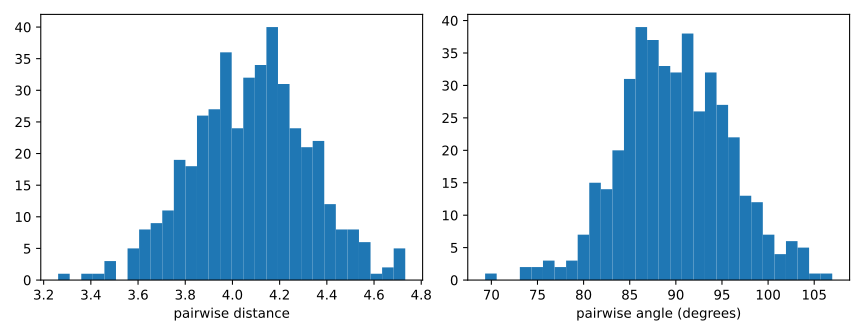
The distances have mean \(4.080\), standard deviation \(0.245\) and range \([3.26,\,4.73]\); the angles have mean \(89.93^\circ\), standard deviation \(5.91^\circ\) and range \([69.3^\circ,\,107.0^\circ]\); the mean norm is \(2.889\). This matches Exercise 2.1 (part 3, shifted cube) with \(d=100\):
\begin{equation*} \begin{aligned} E|\mathbf x-\mathbf y|^2&=\tfrac{d}{6},\quad &\sqrt{100/6}&\approx 4.082,\\ E|\mathbf x|^2&=\tfrac{d}{12},\quad &\sqrt{100/12}&\approx 2.887, \end{aligned} \end{equation*}
and \(|\mathbf x-\mathbf y|^2\) is a sum of \(d\) independent terms, so by the law of large numbers (Theorem 2.4) its relative fluctuation is \(O(1/\sqrt d)\): since \(\operatorname{Var}(x_i-y_i)^2=\frac1{15}-\frac1{36}=\frac7{180}\), the distance has standard deviation \(\approx\sqrt{100\cdot 7/180}\,/\,(2\cdot 4.082)\approx 0.24\). Likewise \(\cos\theta=\mathbf x\cdot\mathbf y/(|\mathbf x||\mathbf y|)\) has mean \(0\) and standard deviation \(\approx\sqrt{d}\,\frac1{12}/\frac{d}{12}=1/\sqrt d=0.1\), i.e. about \(5.7^\circ\) around \(90^\circ\).
Show that for any \(a\ge 1\) there exist distributions for which Markov’s inequality is tight by showing the following:
(1) For each \(a=2,3\), and \(4\) give a probability distribution \(p(x)\) for a nonnegative random variable \(x\) where \(\mathrm{Prob}(x\ge a)=\frac{E(x)}{a}\).
(2) For arbitrary \(a\ge 1\) give a probability distribution for a nonnegative random variable \(x\) where \(\mathrm{Prob}(x\ge a)=\frac{E(x)}{a}\).
Put mass \(\frac1a\) at \(a\) and the rest at \(0\).
(1)
| \(a\) | distribution | \(E(x)\) | \(\mathrm{Prob}(x\ge a)\) | \(E(x)/a\) |
|---|---|---|---|---|
| \(2\) | \(p(0)=\frac12,\ p(2)=\frac12\) | \(1\) | \(\frac12\) | \(\frac12\) |
| \(3\) | \(p(0)=\frac23,\ p(3)=\frac13\) | \(1\) | \(\frac13\) | \(\frac13\) |
| \(4\) | \(p(0)=\frac34,\ p(4)=\frac14\) | \(1\) | \(\frac14\) | \(\frac14\) |
(2) For \(a\ge1\) let \(p(0)=1-\frac1a\) and \(p(a)=\frac1a\); this is a probability distribution because \(0<\frac1a\le 1\), and \(x\ge0\). Then
\begin{equation*} E(x)=a\cdot\tfrac1a=1,\qquad \mathrm{Prob}(x\ge a)=\tfrac1a=\frac{E(x)}{a}, \end{equation*}
so equality holds in Markov’s inequality (Theorem 2.1).
Show that for any \(c\ge 1\) there exist distributions for which Chebyshev’s inequality is tight, in other words, \(\mathrm{Prob}(|x-E(x)|\ge c)=\mathrm{Var}(x)/c^2\).
Take \(p( c)=p(-c)=\frac1{2c^2}\) and \(p(0)=1-\frac1{c^2}\), a probability distribution because \(c\ge1\) gives \(0<\frac1{c^2}\le1\). By symmetry \(E(x)=0\), and
\begin{equation*} \mathrm{Var}(x)=E(x^2)=c^2\cdot\tfrac1{c^2}=1,\qquad \mathrm{Prob}(|x-E(x)|\ge c)=\mathrm{Prob}(x=\pm c)=\tfrac1{c^2}=\frac{\mathrm{Var}(x)}{c^2}, \end{equation*}
so Chebyshev’s inequality (Theorem 2.3) holds with equality.
Let \(x\) be a random variable with probability density \(\frac14\) for \(0\le x\le 4\) and zero elsewhere.
(1) Use Markov’s inequality to bound the probability that \(x\ge 3\).
(2) Make use of \(\mathrm{Prob}(|x|\ge a)=\mathrm{Prob}(x^2\ge a^2)\) to get a tighter bound.
(3) What is the bound using \(\mathrm{Prob}(|x|\ge a)=\mathrm{Prob}(x^r\ge a^r)\)?
The true value is \(\mathrm{Prob}(x\ge3)=\frac14\), and \(x\ge0\) so \(|x|=x\). All three parts use \(E(x^r)=\frac14\int_0^4 t^r\,dt=\frac{4^r}{r+1}\) and Markov’s inequality (Theorem 2.1) applied to the nonnegative variable \(x^r\).
(1) \(\mathrm{Prob}(x\ge3)\le \frac{E(x)}{3}=\frac23\).
(2) \(\mathrm{Prob}(x\ge3)=\mathrm{Prob}(x^2\ge9)\le\frac{E(x^2)}{9}=\frac{16/3}{9}=\frac{16}{27}\approx0.593\).
(3) For \(r>0\),
\begin{equation*} \mathrm{Prob}(x\ge3)=\mathrm{Prob}(x^r\ge3^r)\le\frac{E(x^r)}{3^r}=\frac{(4/3)^r}{r+1}. \end{equation*}
Setting the derivative of \(r\ln\frac43-\ln(r+1)\) to zero gives \(r+1=1/\ln\frac43\), i.e. \(r\approx2.476\), where the bound attains its minimum
\begin{equation*} \frac{(4/3)^r}{r+1}=\tfrac34\,e\,\ln\tfrac43\approx0.587 . \end{equation*}
Among integers, \(r=2\) and \(r=3\) tie at \(\frac{16}{27}\), while \(r=4\) gives \(\frac{256}{405}\approx0.632\) and the bound tends to \(\infty\) as \(r\to\infty\); so no moment bound gets below \(0.587\).
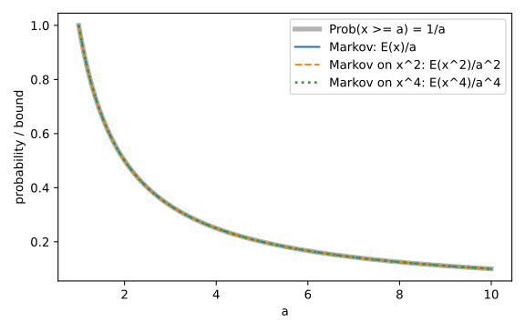
Consider the probability distribution \(p(x=0)=1-\frac1a\) and \(p(x=a)=\frac1a\). Plot the probability that \(x\) is greater than or equal to \(a\) as a function of \(a\) for the bound given by Markov’s inequality and by Markov’s inequality applied to \(x^2\) and \(x^4\).
All three bounds equal the true probability \(\frac1a\) for every \(a\ge1\). Indeed \(E(x^k)=a^k\cdot\frac1a=a^{k-1}\), so Markov’s inequality (Theorem 2.1) applied to \(x^k\) gives
\begin{equation*} \mathrm{Prob}(x\ge a)=\mathrm{Prob}(x^k\ge a^k)\le\frac{E(x^k)}{a^k}=\frac{a^{k-1}}{a^k}=\frac1a, \qquad k=1,2,4, \end{equation*}
and \(\mathrm{Prob}(x\ge a)=p(x=a)=\frac1a\). The plot (for \(1\le a\le10\); numerically the curves differ by at most \(10^{-16}\)) therefore shows four coincident curves:
Consider the probability density function \(p(x)=0\) for \(x<1\) and \(p(x)=c\frac1{x^4}\) for \(x\ge1\).
(1) What should \(c\) be to make \(p\) a legal probability density function?
(2) Generate \(100\) random samples from this distribution. How close is the average of the samples to the expected value of \(x\)?
(1) \(c=3\), since \(\int_1^\infty c\,x^{-4}\,dx=\frac c3\) must equal \(1\).
(2) With seed 0 the sample mean was \(1.4779\), within \(0.022\) of \(E(x)=\frac32\). The relevant moments are
\begin{equation*} E(x)=\int_1^\infty \frac{3}{x^3}\,dx=\frac32,\qquad E(x^2)=\int_1^\infty \frac{3}{x^2}\,dx=3,\qquad \mathrm{Var}(x)=3-\tfrac94=\tfrac34 . \end{equation*}
Samples come from the inverse CDF: \(F(x)=1-x^{-3}\), so \(x=u^{-1/3}\) with \(u\) uniform on \((0,1)\).
import numpy as np
rng = np.random.default_rng(0)
x = rng.uniform(size=100) ** (-1/3)     # inverse CDF of 3/x^4 on [1, inf)
print(x.mean(), x.mean() - 1.5, x.std(ddof=1))
The output was mean \(1.4779\), error \(-0.0221\), sample standard deviation \(0.825\) (largest sample \(7.15\)). The error is of the expected size: the variance is finite, so by the law of large numbers (Theorem 2.4) the average of \(n=100\) samples has standard deviation
\begin{equation*} \sqrt{\mathrm{Var}(x)/n}=\sqrt{0.75/100}\approx0.087, \end{equation*}
and \(|{-0.022}|\) is about a quarter of that.
Exercises 2.8–2.14
Let \(G\) be a \(d\)-dimensional spherical Gaussian with variance \(\frac12\) in each direction, centered at the origin. Derive the expected squared distance to the origin.
\(\mathbb{E}|\mathbf{x}|^2 = d/2\). For \(\mathbf{x}=(x_1,\dots,x_d)\sim G\) each \(x_i \sim N(0,\tfrac12)\), so by linearity
\begin{equation*} \begin{aligned} \mathbb{E}|\mathbf{x}|^2&=\sum_{i=1}^d \mathbb{E}\,x_i^2 =\sum_{i=1}^d \Big(\operatorname{Var}(x_i)+(\mathbb{E}x_i)^2\Big)\\ &=d\cdot\tfrac12=\frac d2 . \end{aligned} \end{equation*}
Consider drawing a random point \(\mathbf{x}\) on the surface of the unit sphere in \(\mathbb{R}^d\). What is the variance of \(x_1\) (the first coordinate of \(\mathbf{x}\))? See if you can give an argument without doing any integrals.
\(\operatorname{Var}(x_1)=1/d\). The uniform distribution on the sphere is invariant under the reflection \(x_1\mapsto -x_1\), so \(\mathbb{E}x_1=0\); it is also invariant under permutations of the coordinates, so \(\mathbb{E}x_1^2=\cdots=\mathbb{E}x_d^2\). Since \(|\mathbf{x}|=1\) always,
\begin{equation*} d\,\mathbb{E}x_1^2=\sum_{i=1}^d\mathbb{E}x_i^2=\mathbb{E}|\mathbf{x}|^2=1 \quad\Longrightarrow\quad \operatorname{Var}(x_1)=\mathbb{E}x_1^2-(\mathbb{E}x_1)^2=\frac1d . \end{equation*}
How large must \(\varepsilon\) be for \(99\%\) of the volume of a \(1000\)-dimensional unit-radius ball to lie in the shell of \(\varepsilon\)-thickness at the surface of the ball?
\(\varepsilon \ge 1-0.01^{1/1000}\approx 0.00459\). The shell is \(S\setminus(1-\varepsilon)S\), and by the scaling identity of Section 2.3, \(\operatorname{vol}((1-\varepsilon)S)=(1-\varepsilon)^{d}\operatorname{vol}(S)\). With \(d=1000\),
\begin{equation*} \begin{aligned} 1-(1-\varepsilon)^{1000}\ge 0.99 &\iff (1-\varepsilon)^{1000}\le 0.01\\ &\iff \varepsilon\ge 1-e^{-\ln 100/1000}=0.0045946\ldots \end{aligned} \end{equation*}
Prove that \(1+x\le e^x\) for all real \(x\). For what values of \(x\) is the approximation \(1+x\approx e^x\) within \(0.01\)?
Let \(g(x)=e^x-1-x\). Then \(g^{\prime}(x)=e^x-1\) is negative for \(x<0\) and positive for \(x>0\), so \(g\) decreases on \((-\infty,0]\), increases on \([0,\infty)\), and
\begin{equation*} g(x)\ge g(0)=0\quad\text{for all }x,\qquad\text{i.e.}\quad 1+x\le e^x . \end{equation*}
Since \(g\ge 0\), the error is \(|e^x-(1+x)|=g(x)\), and by the monotonicity just shown \(\{x: g(x)\le 0.01\}\) is the interval between the two roots of \(e^x-1-x=0.01\). Solving numerically (bisection),
\begin{equation*} -0.1448\le x\le 0.1382 . \end{equation*}
For what value of \(d\) does the volume, \(V(d)\), of a \(d\)-dimensional unit ball take on its maximum? Hint: Consider the ratio \(\frac{V(d)}{V(d-1)}\).
\(d=5\), with \(V(5)=8\pi^2/15\approx 5.264\). By Lemma 2.6, \(V(d)=2\pi^{d/2}/(d\,\Gamma(\frac d2))=\pi^{d/2}/\Gamma(\frac d2+1)\), and \(\Gamma(x+1)=x\Gamma(x)\) gives
\begin{equation*} \frac{V(d)}{V(d-1)}=\frac{\sqrt\pi\,\Gamma(\frac{d+1}{2})}{\Gamma(\frac d2+1)},\qquad \frac{V(d)}{V(d-2)}=\frac{\pi\,\Gamma(\frac d2)}{\Gamma(\frac d2+1)}=\frac{2\pi}{d}. \end{equation*}
From \(V(1)=2\), \(V(2)=\pi\), \(V(3)=\frac43\pi\), \(V(4)=\frac{\pi^2}{2}\), \(V(5)=\frac{8\pi^2}{15}\), \(V(6)=\frac{\pi^3}{6}\) the successive ratios are
\begin{equation*} \frac{V(d)}{V(d-1)}=\frac\pi2,\ \frac43,\ \frac{3\pi}{8},\ \frac{16}{15},\ \frac{5\pi}{16} \qquad(d=2,\dots,6), \end{equation*}
so \(V\) increases up to \(d=5\) and \(V(6)<V(5)\). For \(d\ge 7\) we have \(2\pi/d<1\), so \(V(d)<V(d-2)\); iterating within each parity class,
\begin{equation*} V(d)<V(5)\ (d\ge 7\text{ odd}),\qquad V(d)<V(6)<V(5)\ (d\ge 8\text{ even}). \end{equation*}
Hence \(\max_d V(d)=V(5)\).
A 3-dimensional cube has vertices, edges, and faces. In a \(d\)-dimensional cube, these components are called faces. A vertex is a 0-dimensional face, an edge a 1-dimensional face, etc. (1) For \(0\le k\le d\), how many \(k\)-dimensional faces does a \(d\)-dimensional cube have? (2) What is the total number of faces of all dimensions? The \(d\)-dimensional face is the cube itself which you can include in your count. (3) What is the surface area of a unit cube in \(d\)-dimensions (a unit cube has side-length one in each dimension)? (4) What is the surface area of the cube if the length of each side was 2? (5) Prove that the volume of a unit cube is close to its surface.
Take the cube \([0,1]^d\); a \(k\)-face is obtained by choosing \(k\) free coordinates and fixing each of the other \(d-k\) at \(0\) or \(1\).
(1) \(\binom dk 2^{d-k}\) (choose the free coordinates, then one of \(2^{d-k}\) fixings).
(2) By the binomial theorem,
\begin{equation*} \sum_{k=0}^d\binom dk 2^{d-k}1^k=(2+1)^d=3^d . \end{equation*}
(3) The surface consists of the \(\binom{d}{d-1}2^1=2d\) facets, each a unit \((d-1)\)-cube of area \(1\), so the surface area is \(2d\).
(4) Each of the \(2d\) facets is a \((d-1)\)-cube of side 2, of area \(2^{d-1}\), so the surface area is \(2d\cdot 2^{d-1}=d\,2^d\).
(5) For \(\mathbf{x}\in[0,1]^d\) the distance to the boundary is \(\min_i\min(x_i,1-x_i)\), so the points at distance at least \(\varepsilon\) from the surface form \([\varepsilon,1-\varepsilon]^d\). Using \(1+x\le e^x\) (Exercise 2.11),
\begin{equation*} \operatorname{vol}\big([\varepsilon,1-\varepsilon]^d\big)=(1-2\varepsilon)^d\le e^{-2\varepsilon d}. \end{equation*}
Hence at least a \(1-e^{-2\varepsilon d}\) fraction of the unit volume lies within distance \(\varepsilon\) of the surface; taking \(\varepsilon=c/d\), all but \(e^{-2c}\) of the volume lies within \(c/d\) of the surface.
Consider the portion of the surface area of a unit radius, 3-dimensional ball with center at the origin that lies within a circular cone whose vertex is at the origin. What is the formula for the incremental unit of area when using polar coordinates to integrate the portion of the surface area of the ball that is lying inside the circular cone? What is the formula for the integral? What is the value of the integral if the angle of the cone is \(36^\circ\)? The angle of the cone is measured from the axis of the cone to a ray on the surface of the cone.
\(dA=\sin\theta\,d\theta\,d\phi\), the area is \(2\pi(1-\cos\alpha)\), and for \(\alpha=36^\circ\) it equals \(\pi(3-\sqrt5)/2\approx 1.200\). Put the cone’s axis along the \(z\)-axis and use spherical coordinates with polar angle \(\theta\) (from the axis) and azimuth \(\phi\); on the unit sphere a \(d\theta\) step has length \(d\theta\) and a \(d\phi\) step has length \(\sin\theta\,d\phi\), giving the area element above. The cone of half-angle \(\alpha\) is \(\{\theta\le\alpha\}\), so
\begin{equation*} \begin{aligned} A(\alpha)&=\int_0^{2\pi}\!\!\int_0^{\alpha}\sin\theta\,d\theta\,d\phi=2\pi(1-\cos\alpha),\\ A(36^\circ)&=2\pi\Big(1-\tfrac{1+\sqrt5}{4}\Big)=\frac{\pi(3-\sqrt5)}{2}\approx 1.19998, \end{aligned} \end{equation*}
using \(\cos 36^\circ=\frac{1+\sqrt5}{4}\).
Exercises 2.15–2.21
Consider a unit radius, circular cylinder in 3-dimensions of height one. The top of the cylinder could be an horizontal plane or half of a circular ball. Consider these two possibilities for a unit radius, circular cylinder in 4-dimensions. In 4-dimensions the horizontal plane is 3-dimensional and the half circular ball is 4-dimensional. In each of the two cases, what is the surface area of the top face of the cylinder? You can use \(V(d)\) for the volume of a unit radius, \(d\)-dimension ball and \(A(d)\) for the surface area of a unit radius, \(d\)-dimensional ball. An infinite length, unit radius, circular cylinder in 4-dimensions would be the set \(\{(x_1,x_2,x_3,x_4) \mid x_2^2+x_3^2+x_4^2 \le 1\}\) where the coordinate \(x_1\) is the axis.
Flat top: \(V(3) = \tfrac43\pi\); hemispherical top: \(\tfrac12 A(4) = \pi^2\).
(i) The flat top is the slice \(\{x_1 = 1,\ x_2^2+x_3^2+x_4^2 \le 1\}\), a solid unit 3-ball, so its 3-dimensional measure is \(V(3) = \tfrac43\pi\).
(ii) The rounded top is the boundary of the half 4-ball \(\{x_1 \ge 1,\ (x_1-1)^2+x_2^2+x_3^2+x_4^2 \le 1\}\) minus its flat base, i.e. half of the unit 3-sphere in \(\mathbb{R}^4\); by Lemma 2.6
\begin{equation*} \tfrac12 A(4) = \frac12\cdot\frac{2\pi^{2}}{\Gamma(2)} = \pi^2 . \end{equation*}
Given a \(d\)-dimensional circular cylinder of radius \(r\) and height \(h\): (1) What is the surface area in terms of \(V(d)\) and \(A(d)\)? (2) What is the volume?
(1)
\begin{equation*} \text{area} = h\, r^{d-2} A(d-1) + 2\, r^{d-1} V(d-1). \end{equation*}
(2)
\begin{equation*} \text{volume} = h\, r^{d-1} V(d-1). \end{equation*}
For the cylinder \(\{x : 0 \le x_1 \le h,\ x_2^2+\cdots+x_d^2 \le r^2\}\) the cross-section is a \((d-1)\)-ball of radius \(r\), with volume \(r^{d-1}V(d-1)\) and surface \(r^{d-2}A(d-1)\); the lateral surface is \(h\) times the latter, the two end caps are cross-sections, and the volume is \(h\) times the cross-section.
How does the volume of a ball of radius two behave as the dimension of the space increases? What if the radius was larger than two but a constant independent of \(d\)? What function of \(d\) would the radius need to be for a ball of radius \(r\) to have approximately constant volume as the dimension increases? Hint: you may want to use Stirling’s approximation, \(n! \approx \left(\frac{n}{e}\right)^n\), for factorial.
Every constant radius gives volume tending to \(0\); constant volume needs \(r \approx \sqrt{d/(2\pi e)}\).
A ball of radius \(r\) has volume \(r^d V(d)\), and by Lemma 2.6, \(V(d) = \pi^{d/2}/\Gamma(\tfrac d2+1)\). Stirling with \(n = d/2\) gives
\begin{equation*} r^d V(d) \approx r^d \pi^{d/2}\left(\frac{2e}{d}\right)^{d/2} = \left(\frac{2\pi e\, r^2}{d}\right)^{d/2}. \end{equation*}
- Radius \(2\): the volume is \(\approx (8\pi e/d)^{d/2}\). Exactly, \(r^dV(d)/\big(r^{d-2}V(d-2)\big) = 2\pi r^2/d = 8\pi/d\), which exceeds \(1\) exactly when \(d < 8\pi \approx 25.1\); the volume therefore rises, peaks at \(d = 24\) (volume \(\approx 3.24\times 10^4\)), falls below \(1\) at \(d = 63\), and then tends to \(0\) faster than any exponential (e.g. \(\approx 3.0\times10^{-10}\) at \(d=100\)).
- Constant radius \(r > 2\): the same picture with the peak moved to \(d \approx 2\pi r^2\); the base \(2\pi e r^2/d\) drops below \(1\) once \(d > 2\pi e r^2\), so the volume still tends to \(0\).
- Constant volume: the base must stay at \(1\), i.e.
\begin{equation*} r = \sqrt{\frac{d}{2\pi e}} \approx 0.242\sqrt d . \end{equation*}
If \(\lim_{d\to\infty} V(d) = 0\), the volume of a \(d\)-dimensional ball for sufficiently large \(d\) must be less than \(V(3)\). How can this be if the \(d\)-dimensional ball contains the three dimensional ball?
There is no contradiction: \(V(d)\) and \(V(3)\) are measured in different units, so they cannot be compared.
\(V(3)\) is a 3-dimensional measure (in units of length cubed) and \(V(d)\) is a \(d\)-dimensional measure (in units of length to the \(d\)). The containment does give an inequality, but between \(d\)-dimensional measures: the copy \(\{x : x_4=\cdots=x_d=0,\ x_1^2+x_2^2+x_3^2\le 1\}\) of the 3-ball lies in a 3-dimensional subspace, so its \(d\)-dimensional volume is \(0 \le V(d)\). The numbers \(V(d) < V(3)\) only mean that the \(d\)-ball holds fewer unit \(d\)-cubes than the 3-ball holds unit 3-cubes. The two counts are unrelated: the unit \(d\)-cube \([-\tfrac12,\tfrac12]^d\) has volume \(1\) but its corners are at distance \(\sqrt d/2\), so for large \(d\) it sticks far outside the unit ball.
(1) Write a recurrence relation for \(V(d)\) in terms of \(V(d-1)\) by integrating over \(x_1\). Hint: At \(x_1 = t\), the \((d-1)\)-dimensional volume of the slice is the volume of a \((d-1)\)-dimensional sphere of radius \(\sqrt{1-t^2}\). Express this in terms of \(V(d-1)\) and write down the integral. You need not evaluate the integral. (2) Verify the formula for \(d=2\) and \(d=3\) by integrating and comparing with \(V(2) = \pi\) and \(V(3) = \frac43\pi\).
(1)
\begin{equation*} V(d) = V(d-1)\int_{-1}^{1} (1-t^2)^{\frac{d-1}{2}}\, dt . \end{equation*}
The slice \(\{x_1 = t\}\) of the unit ball is a \((d-1)\)-ball of radius \(\sqrt{1-t^2}\), whose volume is \((\sqrt{1-t^2})^{d-1}V(d-1)\); integrating over \(t \in [-1,1]\) gives the display.
(2) With \(V(1) = 2\) (the interval \([-1,1]\)):
\begin{equation*} \begin{aligned} V(2) &= 2\int_{-1}^{1}\sqrt{1-t^2}\,dt = 2\cdot\frac{\pi}{2} = \pi,\\ V(3) &= \pi\int_{-1}^{1}(1-t^2)\,dt = \pi\left(2-\frac23\right) = \frac43\pi, \end{aligned} \end{equation*}
where \(\int_{-1}^1\sqrt{1-t^2}\,dt = \int_{-\pi/2}^{\pi/2}\cos^2\theta\,d\theta = \pi/2\) by \(t = \sin\theta\).
Consider a unit ball \(A\) centered at the origin and a unit ball \(B\) whose center is at distance \(s\) from the origin. Suppose that a random point \(x\) is drawn from the mixture distribution: “with probability \(1/2\), draw at random from \(A\); with probability \(1/2\), draw at random from \(B\)”. Show that a separation \(s \gg 1/\sqrt{d-1}\) is sufficient so that \(\mathrm{Prob}(x \in A\cap B) = o(1)\); i.e., for any \(\epsilon > 0\) there exists \(c\) such that if \(s \ge c/\sqrt{d-1}\), then \(\mathrm{Prob}(x \in A \cap B) < \epsilon\). In other words, this extent of separation means that nearly all of the mixture distribution is identifiable.
Take \(c \ge 2\) with \(\frac{8}{c}e^{-c^2/8} < \epsilon\); then \(s \ge c/\sqrt{d-1}\) gives (for \(d = 2\), \(s \ge c \ge 2\) makes \(A\cap B\) null, so take \(d \ge 3\)) \(\mathrm{Prob}(x\in A\cap B) \le \frac8c e^{-c^2/8} < \epsilon\).
Let \(u\) be the unit vector with \(B\) centered at \(su\), and \(H = \{x : u\cdot x \ge s/2\}\). Each component is uniform on a ball of volume \(V(d)\), so
\begin{equation*} \mathrm{Prob}(x \in A\cap B) = \tfrac12\frac{\mathrm{vol}(A\cap B)}{V(d)} + \tfrac12\frac{\mathrm{vol}(A\cap B)}{V(d)} = \frac{\mathrm{vol}(A\cap B)}{V(d)} . \end{equation*}
The reflection \(R(x) = x + (s - 2u\cdot x)u\) in the hyperplane \(u\cdot x = s/2\) swaps \(0\) and \(su\), hence maps \(A\cap B\) onto itself and \((A\cap B)\setminus H\) into \((A\cap B)\cap H\). Therefore
\begin{equation*} \begin{aligned} \mathrm{vol}(A\cap B) &\le 2\,\mathrm{vol}(A \cap H) \le 2\,\mathrm{vol}\big(A\cap\{|u\cdot x| \ge s/2\}\big)\\ &\le 2\cdot\frac{2}{c^{\prime}}e^{-c^{\prime\,2}/2}\,V(d), \qquad c^{\prime} = \frac{s\sqrt{d-1}}{2}, \end{aligned} \end{equation*}
by Theorem 2.7 applied in direction \(u\) (rotational symmetry of the ball), which needs \(c^{\prime} \ge 1\) and \(d \ge 3\). If \(s \ge c/\sqrt{d-1}\) then \(c^{\prime} \ge c/2 \ge 1\), and since \(\frac{4}{c^{\prime}}e^{-c^{\prime\,2}/2}\) is decreasing in \(c^{\prime}\),
\begin{equation*} \mathrm{Prob}(x\in A\cap B) \le \frac{4}{c/2}e^{-c^2/8} = \frac8c e^{-c^2/8} < \epsilon . \end{equation*}
Consider the upper hemisphere of a unit-radius ball in \(d\)-dimensions. What is the height of the maximum volume cylinder that can be placed entirely inside the hemisphere? As you increase the height of the cylinder, you need to reduce the cylinder’s radius so that it will lie entirely within the hemisphere.
The height is \(h = 1/\sqrt d\) (with radius \(r = \sqrt{(d-1)/d}\)).
As the statement intends, the cylinder’s axis is the north direction \(x_d\); let its base be a \((d-1)\)-ball of radius \(r\) centred at \((c,a)\) with \(a \ge 0\), and let its height be \(h\). Its farthest point from the origin is on the top rim, so it lies in the hemisphere iff \((|c|+r)^2 + (a+h)^2 \le 1\); taking \(c = 0\), \(a = 0\) loosens this, so the optimal cylinder stands on the flat face, centred, with \(r^2 + h^2 = 1\). By Exercise 2.16 its volume is
\begin{equation*} h\,r^{d-1}V(d-1) = V(d-1)\, h\,(1-h^2)^{\frac{d-1}{2}}, \qquad 0 < h < 1 . \end{equation*}
Maximise \(g(h) = \ln h + \frac{d-1}{2}\ln(1-h^2)\), which is strictly concave:
\begin{equation*} g^{\prime}(h) = \frac1h - \frac{(d-1)h}{1-h^2} = 0 \iff 1 - h^2 = (d-1)h^2 \iff h = \frac{1}{\sqrt d}, \end{equation*}
and then \(r = \sqrt{1 - 1/d}\).
Exercises 2.22–2.28
What is the volume of the maximum size \(d\)-dimensional hypercube that can be placed entirely inside a unit radius \(d\)-dimensional ball?
The volume is \(\left(2/\sqrt{d}\right)^{d} = (4/d)^{d/2}\).
A hypercube of side \(s\) has two opposite vertices \(u, w\) with \(|u-w| = s\sqrt{d}\) (its main diagonal). If the cube lies in the unit ball then both vertices do, so
\begin{equation*} s\sqrt{d} = |u-w| \le |u| + |w| \le 2, \qquad\text{i.e.}\qquad s \le \frac{2}{\sqrt{d}} . \end{equation*}
Conversely the cube \([-1/\sqrt{d},\,1/\sqrt{d}]^d\) has side \(2/\sqrt{d}\) and every point satisfies \(|x|^2 \le d\cdot \frac1d = 1\), so it fits. Hence the largest cube has side \(2/\sqrt d\) and volume
\begin{equation*} \left(\frac{2}{\sqrt d}\right)^{d} = \left(\frac{4}{d}\right)^{d/2}. \end{equation*}
Calculate the ratio of area above the plane \(x_1 = \epsilon\) to the area of the upper hemisphere of a unit radius ball in \(d\)-dimensions for \(\epsilon = 0.001, 0.01, 0.02, 0.03, 0.04, 0.05\) and for \(d = 100\) and \(d = 1{,}000\).
The ratio is
\begin{equation*} R_d(\epsilon) = \frac{\int_\epsilon^1 (1-t^2)^{\frac{d-1}{2}}\,dt}{\int_0^1 (1-t^2)^{\frac{d-1}{2}}\,dt}, \end{equation*}
with the values in the table below (rows “vol” read “area” as the \(d\)-dimensional volume, as in the proof of Theorem 2.7; rows “surf” read it as surface area, which replaces the exponent by \(\frac{d-3}{2}\)).
As in the proof of Theorem 2.7, the slice of the ball at \(x_1 = t\) is a \((d-1)\)-ball of radius \(\sqrt{1-t^2}\), of volume \((1-t^2)^{\frac{d-1}{2}}V(d-1)\); the factor \(V(d-1)\) cancels in the ratio. Substituting \(u = t^2\) turns the numerator and denominator into incomplete and complete Beta integrals, so \(R_d(\epsilon) = 1 - I_{\epsilon^2}\!\left(\tfrac12, \tfrac{d+1}{2}\right)\) (surface: \(1 - I_{\epsilon^2}(\tfrac12, \tfrac{d-1}{2})\)) with \(I\) the regularized incomplete Beta function, evaluated numerically:
| \(\epsilon\) | \(0.001\) | \(0.01\) | \(0.02\) | \(0.03\) | \(0.04\) | \(0.05\) |
|---|---|---|---|---|---|---|
| \(d=100\), vol | 0.9920 | 0.9201 | 0.8411 | 0.7636 | 0.6883 | 0.6160 |
| \(d=100\), surf | 0.9921 | 0.9209 | 0.8426 | 0.7658 | 0.6913 | 0.6195 |
| \(d=1000\), vol | 0.9748 | 0.7518 | 0.5269 | 0.3426 | 0.2056 | 0.1135 |
| \(d=1000\), surf | 0.9748 | 0.7520 | 0.5274 | 0.3430 | 0.2061 | 0.1139 |
Almost all of the volume of a ball in high dimensions lies in a narrow slice of the ball at the equator. However, the narrow slice is determined by the point on the surface of the ball that is designated the North Pole. Explain how this can be true if several different locations are selected for the location of the North Pole giving rise to different equators.
There is no conflict: the equatorial slabs for different poles overlap, and almost all of the volume lies in all of them at once.
Fix poles (unit vectors) \(v_1,\dots,v_k\) and let \(S_j = \{x : |x\cdot v_j| \le c/\sqrt{d-1}\}\) be the slab about the equator of \(v_j\). By rotational symmetry Theorem 2.7 applies to each \(v_j\) (it was proved for \(v = e_1\) only for convenience), so each \(S_j\) misses at most a \(\frac2c e^{-c^2/2}\) fraction of the volume, and by the union bound
\begin{equation*} \begin{aligned} \frac{\mathrm{vol}\big(B \setminus (S_1\cap\cdots\cap S_k)\big)}{\mathrm{vol}(B)} &\le \sum_{j=1}^k \frac{\mathrm{vol}(B\setminus S_j)}{\mathrm{vol}(B)}\\ &\le \frac{2k}{c}\, e^{-c^2/2}. \end{aligned} \end{equation*}
Taking \(c = \sqrt{2\ln(4k)}\) (so \(c \ge 1\)) makes the right side at most \(\frac12\) for every \(d \ge 3\), so more than half the ball lies within \(\sqrt{2\ln (4k)}/\sqrt{d-1}\) of every one of the \(k\) equators simultaneously; for any fixed \(k\) this width tends to \(0\) as \(d\to\infty\). This is exactly the box argument after Theorem 2.8 with the \(d\) coordinate directions as poles.
The low-dimensional picture misleads because there a point near one equator is far from another. In high dimensions a typical point \(x\) of the ball has all its coordinates of size \(O(1/\sqrt d)\) in any orthonormal frame (the Discussion after Theorem 2.8), so \(x\cdot v = O(1/\sqrt d)\) for each fixed direction \(v\): a typical point is nearly orthogonal to every fixed direction, and so it sits near every equator.
Explain how the volume of a ball in high dimensions can simultaneously be in a narrow slice at the equator and also be concentrated in a narrow annulus at the surface of the ball.
The volume lives in the intersection of the slab and the annulus, a thin belt around the equator just under the surface, and that intersection is large because the slab is thin in only one of the \(d\) directions.
Let \(S = \{|x_1| \le c/\sqrt{d-1}\}\) and \(A = \{1-\epsilon \le |x| \le 1\}\). By Section 2.3 the complement of \(A\) holds at most an \(e^{-\epsilon d}\) fraction of the volume, and by Theorem 2.7 (with \(c\ge1\), \(d\ge3\)) the complement of \(S\) holds at most \(\frac2c e^{-c^2/2}\), so
\begin{equation*} \frac{\operatorname{vol}(S\cap A)}{\operatorname{vol}(B)} \;\ge\; 1 - e^{-\epsilon d} - \frac{2}{c}\,e^{-c^2/2}, \end{equation*}
which tends to \(1\) for, e.g., \(\epsilon = \frac{\ln d}{d}\) and \(c = \sqrt{2\ln d}\): both the slab width \(\sqrt{2\ln d}/\sqrt{d-1}\) and the annulus width \(\ln d/d\) go to \(0\).
The two constraints barely interact. A point of \(S\) has \(x_1^2 \le c^2/(d-1) = O\!\left(\tfrac{\ln d}{d}\right)\) in
\begin{equation*} |x|^2 = x_1^2 + (x_2^2 + \cdots + x_d^2), \end{equation*}
so being near the surface is a condition on the other \(d-1\) coordinates, which are free: the slab contains the whole \((d-1)\)-ball \(\{x_1 = 0\}\), whose volume is itself concentrated near its boundary sphere by Section 2.3. In the picture of the Discussion after Theorem 2.8, a typical point looks like \((\pm\frac1{\sqrt d},\dots,\pm\frac1{\sqrt d})\): norm about \(1\) and first coordinate \(O(1/\sqrt d)\) at once.
Generate 500 points uniformly at random on the surface of a unit-radius ball in 50 dimensions. Then randomly generate five additional points. For each of the five new points, calculate a narrow band of width \(\frac{2}{\sqrt{50}}\) at the equator, assuming the point was the North Pole. How many of the 500 points are in each band corresponding to one of the five equators? How many of the points are in all five bands? How wide do the bands need to be for all points to be in all five bands?
With seed 0 the five bands contain \(326, 336, 334, 348, 334\) of the 500 points, \(53\) points lie in all five, and the bands must have width \(1.002 \approx 7.08/\sqrt{50}\) to contain every point.
Points are generated as in Section 2.5 (normalized Gaussian vectors); point \(x\) is in the band of pole \(p\) when \(|x\cdot p| \le 1/\sqrt{50}\):
import numpy as np
rng = np.random.default_rng(0)
d, n = 50, 500
def sphere(m):
    g = rng.standard_normal((m, d))
    return g / np.linalg.norm(g, axis=1, keepdims=True)
X, P = sphere(n), sphere(5)
D = np.abs(X @ P.T)                 # |x . pole|, shape (500, 5)
inband = D <= 1 / np.sqrt(d)        # band of width 2/sqrt(d)
print("per band:", inband.sum(axis=0))
print("in all five:", inband.all(axis=1).sum())
print("width for all:", 2 * D.max())
For a uniform point \(x\) and fixed unit \(p\), \((x\cdot p)^2 \sim \mathrm{Beta}\big(\tfrac12,\tfrac{d-1}{2}\big)\) (the surface version of the slice computation in Theorem 2.7), so
\begin{equation*} \Pr\big(|x\cdot p| \le \tfrac{1}{\sqrt{50}}\big) = I_{1/50}\big(\tfrac12, \tfrac{49}{2}\big) = 0.678, \end{equation*}
predicting \(339\) points per band; given \(x\) the five independent poles act independently, so \(500\cdot 0.678^5 = 71.5\) points are expected in all five (the run’s \(53\) is a low draw). To capture all \(2500\) pairs the half-width must exceed \(\max|x\cdot p|\), which by the union-bound reasoning of Theorem 2.8 is about \(\sqrt{2\ln 2500}/\sqrt{d} \approx 0.56\); the run needed width \(2\max|x\cdot p| = 1.002\), about seven times \(2/\sqrt{50}\).
Place 100 points at random on a \(d\)-dimensional unit-radius ball. Assume \(d\) is large. Pick a random vector and let it define two parallel hyperplanes on opposite sides of the origin that are equal distance from the origin. How close can the hyperplanes be moved and still have at least a \(.99\) probability that all of the 100 points land between them?
Each hyperplane can be brought to distance \(t \approx 3.89/\sqrt d\) from the origin (gap \(\approx 7.8/\sqrt d\)); Theorem 2.7 certifies the slightly larger \(t = 4.13/\sqrt{d-1}\).
Let \(v\) be the unit normal and the hyperplanes \(x\cdot v = \pm t\). By rotational symmetry \(x_i\cdot v\) has the law of the first coordinate \(x_1\) of a uniform point of the ball, whatever \(v\) is, so with \(q(t) = \Pr(|x_1| > t)\) the union bound gives
\begin{equation*} \Pr\big(\exists i : |x_i\cdot v| > t\big) \le 100\, q(t). \end{equation*}
Guaranteed bound. Theorem 2.7 (with \(c\ge 1\), \(d\ge3\)) gives \(q\big(c/\sqrt{d-1}\big) \le \frac2c e^{-c^2/2}\), so it suffices that
\begin{equation*} 100\cdot\frac{2}{c}\,e^{-c^2/2} \le 0.01 \iff \frac{2}{c}\,e^{-c^2/2} \le 10^{-4} \Longleftarrow c \ge 4.13 , \end{equation*}
i.e. \(t = 4.13/\sqrt{d-1}\) works for every \(d \ge 3\).
Sharp value. Given \(v\), the 100 points are independent, so the success probability is exactly \((1-q(t))^{100}\), and
\begin{equation*} (1-q(t))^{100} \ge 0.99 \iff q(t) \le 1 - 0.99^{1/100} = 1.005\times 10^{-4}. \end{equation*}
For large \(d\), \(\sqrt d\,x_1 \to N(0,1)\) (Section 2.5: \(x_1 = \rho\, g_1/|g|\) with \(|g| \approx \sqrt d\) by Theorem 2.9 and \(\rho \to 1\)), so \(q(t) \approx 2\big(1-\Phi(t\sqrt d)\big)\) and the condition becomes \(t\sqrt d \ge \Phi^{-1}(1 - 5.02\times10^{-5}) = 3.89\). The exact Beta law \(x_1^2 \sim \mathrm{Beta}\big(\tfrac12,\tfrac{d+1}{2}\big)\) gives \(t\sqrt d = 3.74,\ 3.87,\ 3.89\) for \(d = 10^2, 10^3, 10^4\).
Let \(\mathbf{x}\) and \(\mathbf{y}\) be \(d\)-dimensional zero mean, unit variance Gaussian vectors. Prove that \(\mathbf{x}\) and \(\mathbf{y}\) are almost orthogonal by considering their dot product.
The dot product is only \(O(\sqrt d)\) while \(|\mathbf x||\mathbf y| \approx d\), so \(\cos\theta = O(1/\sqrt d)\) with high probability (taking \(\mathbf x, \mathbf y\) independent, as intended).
Since the \(2d\) coordinates are independent \(N(0,1)\), the cross terms vanish and
\begin{equation*} \begin{aligned} E(\mathbf x\cdot\mathbf y) &= \sum_{i=1}^d E(x_i)E(y_i) = 0,\\ \operatorname{Var}(\mathbf x\cdot\mathbf y) &= \sum_{i,j} E(x_ix_j)E(y_iy_j) = \sum_{i=1}^d E(x_i^2)E(y_i^2) = d . \end{aligned} \end{equation*}
By Chebyshev’s inequality (Theorem 2.3), for every \(k>0\),
\begin{equation*} \Pr\big(|\mathbf x\cdot\mathbf y| \ge k\sqrt d\big) \le \frac{1}{k^2}. \end{equation*}
By the Gaussian Annulus Theorem (Theorem 2.9) with \(\beta = \sqrt d/2 \le \sqrt d\), each of \(|\mathbf x|, |\mathbf y|\) is at least \(\sqrt d/2\) except with probability \(3e^{-cd/4}\). On the intersection of the three good events, which has probability at least \(1 - \frac1{k^2} - 6e^{-cd/4}\),
\begin{equation*} |\cos\theta| = \frac{|\mathbf x\cdot\mathbf y|}{|\mathbf x|\,|\mathbf y|} \le \frac{k\sqrt d}{d/4} = \frac{4k}{\sqrt d}. \end{equation*}
Taking \(k = d^{1/4}\) gives \(|\cos\theta| \le 4d^{-1/4}\) with probability at least \(1 - d^{-1/2} - 6e^{-cd/4}\), so as \(d\to\infty\) the bound tends to \(0\) and the probability to \(1\): \(\mathbf x\) and \(\mathbf y\) are almost orthogonal, with \(\theta = \frac\pi2 \pm O(k/\sqrt d)\).
Exercises 2.29–2.35
Prove that with high probability, the angle between two random vectors in a high-dimensional space is at least \(45^\circ\). Hint: use Theorem 2.8.
With probability \(1-O(1/d)\) the angle \(\theta\) satisfies \(\cos\theta\le \sqrt{6\ln d/(d-1)}\,/(1-2\ln d/d)^2\), which is below \(1/\sqrt2\) for every \(d\ge 85\), so \(\theta\ge 45^\circ\).
Take the two vectors uniform in the unit ball (the angle depends only on their directions, which are uniform on the sphere also for Gaussian or sphere-uniform vectors). Regard them as \(\mathbf x_1,\mathbf x_2\) among \(n=d\) independent uniform points \(\mathbf x_1,\dots,\mathbf x_d\) of the ball. By Theorem 2.8 with \(n=d\), with probability \(1-O(1/d)\) we have \(|\mathbf x_i|\ge 1-\frac{2\ln d}{d}\) for \(i=1,2\) and \(|\mathbf x_1\cdot\mathbf x_2|\le \frac{\sqrt{6\ln d}}{\sqrt{d-1}}\). On this event
\begin{equation*} \begin{aligned} \cos\theta\le\frac{|\mathbf x_1\cdot\mathbf x_2|}{|\mathbf x_1|\,|\mathbf x_2|} &\le \frac{\sqrt{6\ln d/(d-1)}}{\left(1-2\ln d/d\right)^2} \xrightarrow[d\to\infty]{}0 . \end{aligned} \end{equation*}
The right side is at most \(1/\sqrt2=\cos 45^\circ\) for all \(d\ge 85\) (Check!), hence
\begin{equation*} \operatorname{Prob}\left(\theta\ge 45^\circ\right)\ge 1-O(1/d)\longrightarrow 1 . \end{equation*}
Project the volume of a \(d\)-dimensional ball of radius \(\sqrt d\) onto a line through the center. For large \(d\), give an intuitive argument that the projected volume should behave like a Gaussian.
The projected volume has density proportional to \((1-t^2/d)^{(d-1)/2}\), which tends to \(e^{-t^2/2}\): the projection is asymptotically the standard Gaussian \(N(0,1)\).
Take the line to be the \(x_1\)-axis. As in the proof of Theorem 2.7, the slice \(x_1=t\) of the ball of radius \(\sqrt d\) is a \((d-1)\)-ball of radius \(\sqrt{d-t^2}\), so the projected volume at \(t\in[-\sqrt d,\sqrt d]\) is
\begin{equation*} \begin{aligned} V(d-1)\,(d-t^2)^{\frac{d-1}{2}} &= V(d-1)\,d^{\frac{d-1}{2}}\left(1-\frac{t^2}{d}\right)^{\frac{d-1}{2}},\\ \left(1-\frac{t^2}{d}\right)^{\frac{d-1}{2}} &=\exp\left(\frac{d-1}{2}\ln\left(1-\frac{t^2}{d}\right)\right) \longrightarrow e^{-t^2/2}. \end{aligned} \end{equation*}
Since \(\ln(1-u)\le -u\), the integrand is dominated by \(e^{-t^2(d-1)/(2d)}\le e^{-t^2/4}\) for \(d\ge2\), so its integral tends to \(\int e^{-t^2/2}\,dt=\sqrt{2\pi}\) and the normalized projected density tends to \(\frac{1}{\sqrt{2\pi}}e^{-t^2/2}\).
Intuition: almost all the volume of the ball of radius \(\sqrt d\) lies in a thin shell at radius about \(\sqrt d\) (Section 2.3), which is exactly where a unit-variance spherical Gaussian puts almost all its mass (Theorem 2.9). Both distributions are rotation invariant, so uniform-in-the-ball and \(N(0,I_d)\) are nearly the same distribution, and the projection of \(N(0,I_d)\) on any unit direction is exactly \(N(0,1)\).
(1) Write a computer program that generates \(n\) points uniformly distributed over the surface of a unit-radius \(d\)-dimensional ball. (2) Generate 200 points on the surface of a sphere in 50 dimensions. (3) Create several random lines through the origin and project the points onto each line. Plot the distribution of points on each line. (4) What does your result from (3) say about the surface area of the sphere in relation to the lines, i.e., where is the surface area concentrated relative to each line?
(1) Normalize spherical Gaussian vectors, as in Section 2.5: \(\mathbf x=\mathbf g/|\mathbf g|\) with \(\mathbf g\sim N(0,I_d)\) is uniform on the unit sphere because the Gaussian density is rotation invariant.
import numpy as np, matplotlib.pyplot as plt
rng = np.random.default_rng(2031)
def sphere_points(n, d):
    g = rng.standard_normal((n, d))
    return g / np.linalg.norm(g, axis=1, keepdims=True)
X = sphere_points(200, 50)                      # part 2
fig, axes = plt.subplots(1, 4, figsize=(11, 2.8), sharey=True)
for k, ax in enumerate(axes):                   # part 3
    u = sphere_points(1, 50)[0]                 # random line through 0
    p = X @ u                                   # projections onto the line
    print(k, p.mean(), p.std(), abs(p).max())
    ax.hist(p, bins=np.linspace(-1, 1, 41))
    ax.set_xlim(-1, 1); ax.set_title(f'line {k+1}')
plt.show()
(2) The call sphere_points(200, 50) produces the \(200\times 50\) matrix X of points.
(3) For four random lines the projections had standard deviations \(0.149,\ 0.133,\ 0.144,\ 0.135\) (against \(1/\sqrt{50}=0.141\)), means within \(0.016\) of \(0\), and largest absolute value between \(0.40\) and \(0.48\). Between \(92.5\%\) and \(98\%\) of the points fell within \(2/\sqrt{50}=0.283\) of the origin. All four histograms are bell-shaped around \(0\) and leave the ends \(\pm1\) of the line empty.
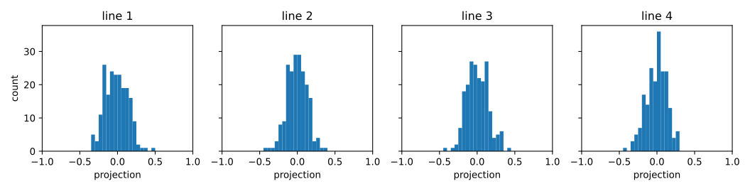
(4) Relative to every line, the surface area is concentrated near the equator perpendicular to it: the projection onto a unit direction is approximately \(N(0,1/d)\), so almost all of the area lies within \(O(1/\sqrt d)\) of the hyperplane through the origin orthogonal to the line, and the polar caps near \(\pm1\) carry almost none (Theorem 2.7 and Section 2.4; the surface analogue holds by the same calculation).
If one generates points in \(d\)-dimensions with each coordinate a unit variance Gaussian, the points will approximately lie on the surface of a sphere of radius \(\sqrt d\). (1) What is the distribution when the points are projected onto a random line through the origin? (2) If one uses a Gaussian with variance four, where in \(d\)-space will the points lie?
(1) The projection is exactly \(N(0,1)\), whatever the line. For a unit vector \(\mathbf u\) along the line and \(\mathbf x\) with i.i.d. \(N(0,1)\) coordinates,
\begin{equation*} \mathbf u\cdot\mathbf x=\sum_{i=1}^d u_ix_i \sim N\left(0,\sum_{i=1}^d u_i^2\right)=N(0,1), \end{equation*}
a linear combination of independent Gaussians (this is the computation in the proof of Theorem 2.10). If \(\mathbf u\) is itself random and independent of \(\mathbf x\), conditioning on \(\mathbf u\) gives \(N(0,1)\) for every value of \(\mathbf u\), so the projection is still \(N(0,1)\). (2) Near the sphere of radius \(2\sqrt d\). Writing \(\mathbf x=2\mathbf z\) with \(\mathbf z\sim N(0,I_d)\), we get \(E|\mathbf x|^2=4d\), and by Theorem 2.9 applied to \(\mathbf z\), for \(\beta\le\sqrt d\),
\begin{equation*} \operatorname{Prob}\left(\bigl||\mathbf x|-2\sqrt d\bigr|\le 2\beta\right) \ge 1-3e^{-c\beta^2}, \end{equation*}
so the points lie in an annulus of width \(O(1)\) around radius \(2\sqrt d\).
Randomly generate 100 points on the surface of a sphere in 3-dimensions and in 100-dimensions. Create a histogram of all distances between the pairs of points in both cases.
In 3 dimensions the \(4950\) pairwise distances spread over all of \([0,2]\) with density rising linearly; in 100 dimensions they cluster tightly at \(\sqrt2\).
import numpy as np, matplotlib.pyplot as plt
from scipy.spatial.distance import pdist
rng = np.random.default_rng(2033)
fig, axes = plt.subplots(1, 2, figsize=(9, 3), sharex=True)
for ax, d in zip(axes, (3, 100)):
    g = rng.standard_normal((100, d))
    X = g / np.linalg.norm(g, axis=1, keepdims=True)   # uniform on sphere
    D = pdist(X)                                        # all 4950 distances
    print(d, D.mean(), D.std(), D.min(), D.max())
    ax.hist(D, bins=np.linspace(0, 2, 51), density=True)
    ax.set_title(f'd = {d}')
plt.show()
The run gave:
| \(d\) | mean | std. dev. | min | max |
|---|---|---|---|---|
| 3 | 1.334 | 0.474 | 0.025 | 2.000 |
| 100 | 1.410 | 0.070 | 1.159 | 1.650 |
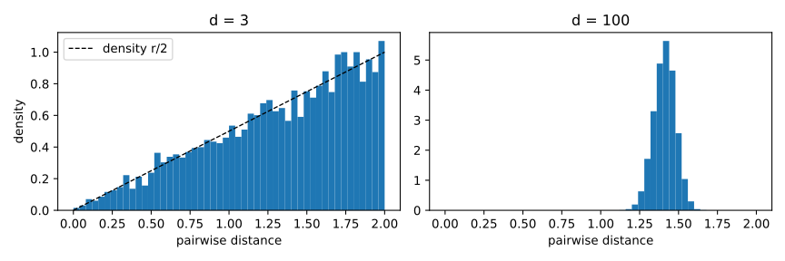
Both match the exact picture. For unit vectors \(|\mathbf x-\mathbf y|^2=2-2\,\mathbf x\cdot\mathbf y\). In \(d=3\), \(\mathbf x\cdot\mathbf y\) is uniform on \([-1,1]\) (Archimedes), so \(r=|\mathbf x-\mathbf y|\) has density \(r/2\) on \([0,2]\), with mean \(4/3\) and standard deviation \(\sqrt{2-16/9}=0.471\) (the dashed line in the left panel). In \(d=100\), \(\mathbf x\cdot\mathbf y\) is the projection of \(\mathbf y\) on the direction \(\mathbf x\), approximately \(N(0,1/d)\) (Exercises 2.31 and 2.32), so
\begin{equation*} r=\sqrt{2-2\,\mathbf x\cdot\mathbf y} \approx\sqrt2-\frac{\mathbf x\cdot\mathbf y}{\sqrt2}, \qquad \operatorname{sd}( r)\approx\frac{1}{\sqrt{2d}}=0.0707 . \end{equation*}
We have claimed that a randomly generated point on a ball lies near the equator of the ball, independent of the point picked to be the North Pole. Is the same claim true for a randomly generated point on a cube? To test this claim, randomly generate ten \(\pm1\) valued vectors in 128 dimensions. Think of these ten vectors as ten choices for the North Pole. Then generate some additional \(\pm1\) valued vectors. To how many of the original vectors is each of the new vectors close to being perpendicular; that is, how many of the equators is each new vector close to?
Yes: a new random vertex is close to perpendicular to essentially all ten poles, on average \(9.6\) of the ten within \(10^\circ\) of \(90^\circ\) and \(9.97\) of the ten within \(15^\circ\).
For a fixed pole \(\mathbf p\in\{\pm1\}^d\) and an independent uniform \(\mathbf q\in\{\pm1\}^d\), the products \(p_iq_i\) are independent uniform \(\pm1\) variables, whatever \(\mathbf p\) is, so
\begin{equation*} \cos\theta=\frac{\mathbf p\cdot\mathbf q}{d}=\frac1d\sum_{i=1}^d p_iq_i, \qquad E\cos\theta=0,\qquad \operatorname{Var}\cos\theta=\frac1d , \end{equation*}
and by Chebyshev (Theorem 2.3) \(\operatorname{Prob}(|\cos\theta|>t/\sqrt d)\le 1/t^2\); exactly, since \((\mathbf p\cdot\mathbf q+d)/2\sim\mathrm{Bin}(d,1/2)\), for \(d=128\) the probabilities of \(|\cos\theta|\le 2/\sqrt d=0.177\) and \(|\cos\theta|\le 3/\sqrt d=0.265\) are \(0.958\) and \(0.997\). As for the ball, the claim holds for every choice of pole.
Experiment (seed 2034): ten random poles, \(1000\) new random \(\pm1\) vectors, \(d=128\). The \(10\,000\) cosines had standard deviation \(0.0879\) (theory \(1/\sqrt{128}=0.0884\)) and largest absolute value \(0.359\), so every angle lay between \(68.9^\circ\) and \(111.1^\circ\). Counting, for each new vector, the poles it is close to perpendicular to:
| closeness | 6 | 7 | 8 | 9 | 10 | average |
|---|---|---|---|---|---|---|
| \(\lvert\cos\theta\rvert\le 2/\sqrt d\) (within \(10.2^\circ\)) | 1 | 6 | 45 | 266 | 682 | 9.62 |
| \(\lvert\cos\theta\rvert\le 3/\sqrt d\) (within \(15.4^\circ\)) | 0 | 0 | 0 | 27 | 973 | 9.97 |
The averages agree with \(10\times0.958=9.58\) and \(10\times0.997=9.97\).
Define the equator of a \(d\)-dimensional unit cube to be the hyperplane \(\left\{\mathbf x \,\middle|\, \sum_{i=1}^d x_i=\frac d2\right\}\). (1) Are the vertices of a unit cube concentrated close to the equator? (2) Is the volume of a unit cube concentrated close to the equator? (3) Is the surface area of a unit cube concentrated close to the equator?
Yes to all three: in each case all but a \(O(1/t^2)\) fraction lies within distance \(t\) of the equator, while the cube reaches distance \(\sqrt d/2\) from it (at the vertices \(\mathbf 0\) and \(\mathbf 1\)).
The cube is \([0,1]^d\) and the distance from \(\mathbf x\) to the equator is \(|S-d/2|/\sqrt d\) with \(S=\sum_i x_i\). Pick a point uniformly from the relevant set; by Chebyshev (Theorem 2.3),
\begin{equation*} \operatorname{Prob}\left(\frac{|S-d/2|}{\sqrt d}\ge t\right) \le\frac{\operatorname{Var}S}{t^2d} \qquad\text{when } ES=\frac d2 . \end{equation*}
(1) A uniform vertex has independent coordinates \(x_i\in\{0,1\}\) with \(\operatorname{Var}x_i=\frac14\), so \(ES=\frac d2\), \(\operatorname{Var}S=\frac d4\), and all but a \(\frac{1}{4t^2}\) fraction of the \(2^d\) vertices lie within distance \(t\) of the equator. (2) A uniform point of the cube has independent \(x_i\sim U[0,1]\) with \(\operatorname{Var}x_i=\frac1{12}\), so \(\operatorname{Var}S=\frac d{12}\) and all but a \(\frac{1}{12t^2}\) fraction of the volume lies within distance \(t\) of the equator. (3) The surface is the union of the \(2d\) facets \(\{x_i=b\}\), \(b\in\{0,1\}\), each of area \(1\), so it suffices to treat one facet. On it \(S=b+\sum_{j\ne i}x_j\) with the \(d-1\) free coordinates uniform, so \(ES=\frac d2\pm\frac12\), \(\operatorname{Var}S=\frac{d-1}{12}\), and for \(t>\frac{1}{2\sqrt d}\)
\begin{equation*} \begin{aligned} \operatorname{Prob}\left(\frac{|S-d/2|}{\sqrt d}\ge t\right) &\le\operatorname{Prob}\left(|S-ES|\ge t\sqrt d-\tfrac12\right)\\ &\le\frac{(d-1)/12}{\left(t\sqrt d-\frac12\right)^2} \le\frac{1}{12\left(t-\frac1{2\sqrt d}\right)^2}. \end{aligned} \end{equation*}
Averaging over the facets, all but this fraction of the surface area lies within distance \(t\) of the equator.
Exercises 2.36–2.42
Consider a nonorthogonal basis \(\mathbf{e_1},\mathbf{e_2},\dots,\mathbf{e_d}\). The \(\mathbf{e_i}\) are a set of linearly independent unit vectors that span the space.
(1) Prove that the representation of any vector in this basis is unique. (2) Calculate the squared length of \(\mathbf{z}=\left(\frac{\sqrt2}{2},1\right)_e\) where \(\mathbf{z}\) is expressed in the basis \(\mathbf{e_1}=(1,0)\) and \(\mathbf{e_2}=\left(-\frac{\sqrt2}{2},\frac{\sqrt2}{2}\right)\). (3) If \(\mathbf{y}=\sum_i a_i\mathbf{e_i}\) and \(\mathbf{z}=\sum_i b_i\mathbf{e_i}\), with \(0<a_i<b_i\), is it necessarily true that the length of \(\mathbf{z}\) is greater than the length of \(\mathbf{y}\)? Why or why not? (4) Consider the basis \(\mathbf{e_1}=(1,0)\) and \(\mathbf{e_2}=\left(-\frac{\sqrt2}{2},\frac{\sqrt2}{2}\right)\).
- (a) What is the representation of the vector \((0,1)\) in the basis \((\mathbf{e_1},\mathbf{e_2})\)?
- (b) What is the representation of the vector \(\left(\frac{\sqrt2}{2},\frac{\sqrt2}{2}\right)\)?
- (c) What is the representation of the vector \((1,2)\)?
(The accompanying figure shows three copies of the axes with \(\mathbf{e_1}\) along the positive \(x\)-axis and \(\mathbf{e_2}\) at \(135^\circ\), together with the vectors \((0,1)\), \(\left(\frac{\sqrt2}{2},\frac{\sqrt2}{2}\right)\) and \((1,2)\) respectively.)
(1) If \(\mathbf{v}=\sum_i a_i\mathbf{e_i}=\sum_i b_i\mathbf{e_i}\) then \(\sum_i (a_i-b_i)\mathbf{e_i}=\mathbf{0}\), so linear independence forces \(a_i=b_i\) for every \(i\).
(2) \(|\mathbf{z}|^2=\frac12\):
\begin{equation*} \begin{aligned} \mathbf{z}&=\tfrac{\sqrt2}{2}(1,0)+\left(-\tfrac{\sqrt2}{2},\tfrac{\sqrt2}{2}\right) =\left(0,\tfrac{\sqrt2}{2}\right),\\ |\mathbf{z}|^2&=\tfrac12 . \end{aligned} \end{equation*}
(3) No: the cross terms \(2a_ia_j\,\mathbf{e_i}\cdot\mathbf{e_j}\) in \(|\sum_i a_i\mathbf{e_i}|^2\) can be negative. In the basis of part 2 take
\begin{equation*} \begin{aligned} \mathbf{y}&=\tfrac{\sqrt2}{10}\mathbf{e_1}+\mathbf{e_2} =\left(-\tfrac{2\sqrt2}{5},\tfrac{\sqrt2}{2}\right), &|\mathbf{y}|^2&=\tfrac{41}{50},\\ \mathbf{z}&=\tfrac{3\sqrt2}{5}\mathbf{e_1}+\tfrac65\,\mathbf{e_2} =\left(0,\tfrac{3\sqrt2}{5}\right), &|\mathbf{z}|^2&=\tfrac{36}{50}. \end{aligned} \end{equation*}
Here \(0<\frac{\sqrt2}{10}<\frac{3\sqrt2}{5}\) and \(0<1<\frac65\), yet \(|\mathbf{z}|<|\mathbf{y}|\).
(4) Solving \((x,y)=a_1\mathbf{e_1}+a_2\mathbf{e_2}=\left(a_1-\frac{\sqrt2}{2}a_2,\ \frac{\sqrt2}{2}a_2\right)\) gives
\begin{equation*} a_2=\sqrt2\,y,\qquad a_1=x+y . \end{equation*}
- (a) \((0,1)=1\cdot\mathbf{e_1}+\sqrt2\,\mathbf{e_2}\), i.e. \((1,\sqrt2)_e\).
- (b) \(\left(\frac{\sqrt2}{2},\frac{\sqrt2}{2}\right)=\sqrt2\,\mathbf{e_1}+1\cdot\mathbf{e_2}\), i.e. \((\sqrt2,1)_e\).
- (c) \((1,2)=3\,\mathbf{e_1}+2\sqrt2\,\mathbf{e_2}\), i.e. \((3,2\sqrt2)_e\).
Generate 20 points uniformly at random on a 900-dimensional sphere of radius 30. Calculate the distance between each pair of points. Then, select a method of projection and project the data onto subspaces of dimension \(k=100,50,10,5,4,3,2,1\) and calculate the difference between \(\sqrt k\) times the original distances and the new pair-wise distances. For each value of \(k\) what is the maximum difference as a percent of \(\sqrt k\)?
With the Gaussian projection \(f(\mathbf v)=(\mathbf u_1\cdot\mathbf v,\dots,\mathbf u_k\cdot\mathbf v)\) of Section 2.7 (seed 0), the maximum over the \(\binom{20}{2}=190\) pairs of the relative error \(\big||f(\mathbf v_i)-f(\mathbf v_j)|-\sqrt k\,|\mathbf v_i-\mathbf v_j|\big|/(\sqrt k\,|\mathbf v_i-\mathbf v_j|)\) is:
| \(k\) | 100 | 50 | 10 | 5 | 4 | 3 | 2 | 1 |
|---|---|---|---|---|---|---|---|---|
| max error (%) | 22.9 | 28.6 | 57.7 | 88.2 | 81.5 | 85.6 | 119.9 | 189.4 |
| median error (%) | 5.1 | 6.0 | 16.2 | 20.0 | 20.7 | 26.6 | 34.0 | 49.3 |
import numpy as np
from scipy.spatial.distance import pdist
rng = np.random.default_rng(0)
d, n = 900, 20
X = rng.standard_normal((n, d))
X = 30 * X / np.linalg.norm(X, axis=1, keepdims=True)   # uniform on sphere of radius 30
D = pdist(X)                                             # original distances
for k in [100, 50, 10, 5, 4, 3, 2, 1]:
    U = rng.standard_normal((k, d))                      # rows u_1, ..., u_k
    Dk = pdist(X @ U.T)                                  # |f(v_i) - f(v_j)|
    rel = np.abs(Dk - np.sqrt(k) * D) / (np.sqrt(k) * D)
    print(k, 100 * rel.max(), 100 * np.median(rel))
The original distances lie in \([40.8,44.2]\), near \(30\sqrt2\) (Theorem 2.8). For fixed \(\mathbf w=\mathbf v_i-\mathbf v_j\) the vector \(f(\mathbf w)/|\mathbf w|\) is standard Gaussian in \(\mathbb R^k\) (proof of Theorem 2.10), so its length is \(\sqrt k\pm O(1)\) by Theorem 2.9 and the relative error has standard deviation about \(1/\sqrt{2k}\) (\(7\%\) at \(k=100\)): the error decays like \(1/\sqrt k\), as the Johnson-Lindenstrauss Lemma (Theorem 2.11) predicts, and is useless for \(k\le5\).
In \(d\) dimensions there are exactly \(d\) unit vectors that are pairwise orthogonal. However, if you wanted a set of vectors that were almost orthogonal you might squeeze in a few more. For example, in 2 dimensions if almost orthogonal meant at least 45 degrees apart, you could fit in three almost orthogonal vectors. Suppose you wanted to find 1000 almost orthogonal vectors in 100 dimensions. Here are two ways you could do it:
(1) Begin with 1,000 orthonormal 1,000-dimensional vectors, and then project them to a random 100-dimensional space. (2) Generate 1000 100-dimensional random Gaussian vectors.
Implement both ideas and compare them to see which does a better job.
Both methods give 1000 vectors pairwise more than \(60^\circ\) apart; the projection method is slightly better on every measure. Over the \(\binom{1000}{2}=499{,}500\) pairs (seed 0, angles measured after normalising):
| method | max \(\lvert\cos\theta\rvert\) | min angle | RMS \(\lvert\cos\theta\rvert\) | pairs below \(80^\circ\) |
|---|---|---|---|---|
| 1. project \(\mathbf e_1,\dots,\mathbf e_{1000}\) | 0.442 | \(63.8^\circ\) | 0.0950 | 6.7% |
| 2. Gaussian vectors | 0.456 | \(62.9^\circ\) | 0.0999 | 8.2% |
import numpy as np
rng = np.random.default_rng(0)
def stats(V):
    V = V / np.linalg.norm(V, axis=1, keepdims=True)
    C = np.abs(V @ V.T)[np.triu_indices(len(V), 1)]
    ang = np.degrees(np.arccos(C))
    return C.max(), ang.min(), np.sqrt((C**2).mean()), (ang < 80).mean()
Q, _ = np.linalg.qr(rng.standard_normal((1000, 100)))  # orthonormal basis of a random subspace
A = np.eye(1000) @ Q            # method 1: row i = coordinates of the projection of e_i
B = rng.standard_normal((1000, 100))                    # method 2
print(stats(A)); print(stats(B))
For method 2, \(E\cos^2\theta=1/100\) for independent Gaussian directions (Section 2.4.2), so the RMS is \(0.1\). For method 1 the rows \(\mathbf q_i\) of \(Q\) form a tight frame, \(\sum_i\mathbf q_i\mathbf q_i^T=Q^TQ=I_{100}\), hence
\begin{equation*} \sum_{i,j}(\mathbf q_i\cdot\mathbf q_j)^2=\operatorname{tr}\big((QQ^T)^2\big)=\operatorname{tr}(QQ^T)=100, \end{equation*}
the minimum possible for a rank-100 Gram matrix of trace 100; with \(|\mathbf q_i|^2\approx\frac1{10}\) the average off-diagonal \(\cos^2\theta\) is about \(\frac{9}{999}\), RMS \(0.0949\), matching the observed \(0.0950\).
Suppose there is an object moving at constant velocity along a straight line. You receive the gps coordinates corrupted by Gaussian noise every minute. How do you estimate the current position?
Fit the line \(\mathbf x(t)=\mathbf a+\mathbf b\,t\) to all readings by least squares and report \(\hat{\mathbf a}+\hat{\mathbf b}\,n\). With readings \(\mathbf y_t=\mathbf a+\mathbf b t+\boldsymbol\eta_t\) at minutes \(t=1,\dots,n\) and independent spherical noise \(\boldsymbol\eta_t\sim N(\mathbf 0,\sigma^2I)\), the likelihood is
\begin{equation*} c\,\exp\Big(-\frac{1}{2\sigma^2}\sum_{t=1}^n|\mathbf y_t-\mathbf a-\mathbf b t|^2\Big), \end{equation*}
so, exactly as in Section 2.9, the maximum likelihood \((\mathbf a,\mathbf b)\) minimises the sum of squared distances. Setting the gradient to zero (as in Lemma 2.12), with \(\bar t=\frac{n+1}{2}\) and \(\bar{\mathbf y}=\frac1n\sum_t\mathbf y_t\),
\begin{equation*} \begin{aligned} \hat{\mathbf b}&=\frac{\sum_t (t-\bar t)(\mathbf y_t-\bar{\mathbf y})}{\sum_t (t-\bar t)^2},\qquad \hat{\mathbf a}=\bar{\mathbf y}-\hat{\mathbf b}\,\bar t,\\ \hat{\mathbf x}(n)&=\bar{\mathbf y}+\tfrac{n-1}{2}\,\hat{\mathbf b}. \end{aligned} \end{equation*}
This is unbiased, and since \(\sum_t(t-\bar t)^2=\frac{n(n^2-1)}{12}\) each coordinate has variance
\begin{equation*} \begin{aligned} \sigma^2\Big(\frac1n+\frac{(n-\bar t)^2}{\sum_t(t-\bar t)^2}\Big) &=\sigma^2\Big(\frac1n+\frac{3(n-1)}{n(n+1)}\Big)\\ &=\frac{2(2n-1)}{n(n+1)}\,\sigma^2\approx\frac{4\sigma^2}{n}, \end{aligned} \end{equation*}
far below the variance \(\sigma^2\) of the latest reading alone.
(1) What is the maximum size rectangle that can be fitted under a unit variance Gaussian? (2) What unit area rectangle best approximates a unit variance Gaussian if one measures goodness of fit by the symmetric difference of the Gaussian and the rectangle?
Write \(\varphi(x)=\frac{1}{\sqrt{2\pi}}e^{-x^2/2}\) and \(\Phi\) for its distribution function.
(1) The rectangle \([-1,1]\times[0,\varphi(1)]\), of area \(2\varphi(1)=\sqrt{2/(\pi e)}\approx0.4839\). A rectangle \([l,l+w]\times[0,h]\) lies under the curve iff \(h\le\min\big(\varphi(l),\varphi(l+w)\big)\) (\(\varphi\) is unimodal), and one endpoint is at distance at least \(w/2\) from \(0\), so
\begin{equation*} \text{area}\le w\,\varphi(w/2)=2a\varphi(a)\quad(a=w/2),\qquad \frac{d}{da}\,2a\varphi(a)=2(1-a^2)\varphi(a), \end{equation*}
which is positive for \(a<1\) and negative for \(a>1\); the maximum is at \(a=1\).
(2) The rectangle \([-a,a]\times[0,\frac1{2a}]\) with \(a\approx1.486\) (width \(2.973\), height \(0.3364\)), whose symmetric difference with the Gaussian is about \(0.370\). Both regions have area \(1\), so
\begin{equation*} |\,\text{Gaussian}\ \triangle\ \text{rectangle}\,|=\int|\varphi-R|=2-2\int\min(\varphi,R)\,dx, \end{equation*}
and we maximise the overlap. For fixed width \(w\) and height \(h=1/w\) the overlap \(\int_l^{l+w}\min(\varphi,h)\) integrates the symmetric unimodal function \(\min(\varphi,h)\) over a window of length \(w\), which is largest for the centred window \(l=-a\). Since part 1 rules out \(h\le\varphi(a)\), two cases remain:
- (i) \(h\ge\varphi(0)\), i.e. \(a\le\sqrt{\pi/2}\): overlap \(=2\Phi(a)-1\), increasing in \(a\), so not optimal;
- (ii) \(h<\varphi(0)\): with \(\varphi( c)=h=\frac1{2a}\), \(0<c<a\), overlap
\begin{equation*} G(a)=2ch+2\big(\Phi(a)-\Phi( c)\big). \end{equation*}
The \(c\)-derivative \(2h-2\varphi( c)\) vanishes, so
\begin{equation*} \begin{aligned} G^{\prime}(a)=2\varphi(a)-\frac{c}{a^2}=0&\iff 2a^2\varphi(a)=c,\\ c&=\sqrt{2\ln\frac{2a}{\sqrt{2\pi}}}. \end{aligned} \end{equation*}
Solving numerically gives \(a=1.4864\), \(c=0.5841\), \(h=0.3364\), \(G=0.8149\), so the symmetric difference is \(2-2G=0.3701\) (confirmed by direct numerical integration, which also increases when the rectangle is shifted or rescaled).
Let \(x_1,x_2,\dots,x_n\) be independent samples of a random variable \(x\) with mean \(\mu\) and variance \(\sigma^2\). Let \(m_s=\frac1n\sum_{i=1}^n x_i\) be the sample mean. Suppose one estimates the variance using the sample mean rather than the true mean, that is,
\begin{equation*} \sigma_s^2=\frac1n\sum_{i=1}^n(x_i-m_s)^2 . \end{equation*}
Prove that \(E(\sigma_s^2)=\frac{n-1}{n}\sigma^2\) and thus one should have divided by \(n-1\) rather than \(n\).
Hint: First calculate the variance of the sample mean and show that \(\operatorname{var}(m_s)=\frac1n\operatorname{var}(x)\). Then calculate \(E(\sigma_s^2)=E\big[\frac1n\sum_{i=1}^n(x_i-m_s)^2\big]\) by replacing \(x_i-m_s\) with \((x_i-\mu)-(m_s-\mu)\).
By independence the variances add, so
\begin{equation*} \operatorname{var}(m_s)=\frac1{n^2}\sum_{i=1}^n\operatorname{var}(x_i)=\frac{\sigma^2}{n}, \qquad E(m_s)=\mu . \end{equation*}
Using \(x_i-m_s=(x_i-\mu)-(m_s-\mu)\) and \(\sum_i(x_i-\mu)=n(m_s-\mu)\),
\begin{equation*} \begin{aligned} \sum_{i=1}^n(x_i-m_s)^2&=\sum_i(x_i-\mu)^2-2(m_s-\mu)\sum_i(x_i-\mu)+n(m_s-\mu)^2\\ &=\sum_i(x_i-\mu)^2-n(m_s-\mu)^2 , \end{aligned} \end{equation*}
hence
\begin{equation*} E(\sigma_s^2)=\frac1n\Big(n\sigma^2-n\operatorname{var}(m_s)\Big) =\frac{n-1}{n}\,\sigma^2 . \end{equation*}
Therefore \(\frac{1}{n-1}\sum_i(x_i-m_s)^2=\frac{n}{n-1}\sigma_s^2\) has expectation exactly \(\sigma^2\), i.e. dividing by \(n-1\) gives an unbiased estimator.
Generate ten values by a Gaussian probability distribution with zero mean and variance one. What is the center determined by averaging the points? What is the variance? In estimating the variance, use both the real center and the estimated center. When using the estimated center to estimate the variance, use both \(n=10\) and \(n=9\). How do the three estimates compare?
With seed 0 the ten values are
\begin{equation*} 0.126,\ -0.132,\ 0.640,\ 0.105,\ -0.536,\ 0.362,\ 1.304,\ 0.947,\ -0.704,\ -1.265, \end{equation*}
the averaged center is \(m=0.0847\), and the three variance estimates are
\begin{equation*} \begin{aligned} \tfrac1{10}\textstyle\sum_i x_i^2&=0.5566 &&\text{(real center 0)},\\ \tfrac1{10}\textstyle\sum_i (x_i-m)^2&=0.5494 &&\text{(estimated center, }n=10),\\ \tfrac1{9}\textstyle\sum_i (x_i-m)^2&=0.6105 &&\text{(estimated center, }n=9). \end{aligned} \end{equation*}
import numpy as np
rng = np.random.default_rng(0)
x = rng.standard_normal(10)
m = x.mean()
print(m, (x**2).sum() / 10, ((x - m)**2).sum() / 10, ((x - m)**2).sum() / 9)
X = rng.standard_normal((100000, 10)); M = X.mean(1, keepdims=True)   # repeat 100000 times
for v in (X**2).mean(1), ((X - M)**2).sum(1) / 10, ((X - M)**2).sum(1) / 9:
    print(v.mean(), ((v - 1)**2).mean())
The estimated-center sum is always the smaller one, by Lemma 2.12 (the centroid minimises the sum of squared distances); precisely \(\sum_i(x_i-m)^2=\sum_i x_i^2-10m^2=5.566-0.072=5.494\). One sample of ten is too noisy to rank the estimators (all three are well below the true value \(1\) here), so the run was repeated \(100{,}000\) times:
| estimator | mean | mean squared error | theory (mean, MSE) |
|---|---|---|---|
| real center, divide by 10 | 1.0013 | 0.2007 | \(1\), \(\frac{2}{10}\) |
| estimated center, divide by 10 | 0.9016 | 0.1905 | \(\frac{9}{10}\), \(\frac{19}{100}\) |
| estimated center, divide by 9 | 1.0018 | 0.2232 | \(1\), \(\frac{2}{9}\) |
Dividing by \(10\) after estimating the center is biased low by the factor \(\frac{n-1}{n}=0.9\) of Exercise 2.41; dividing by \(9\) removes the bias, at the price of slightly larger variance. (Theory column: \(\sum_i x_i^2\sim\chi^2_{10}\), \(\sum_i(x_i-m)^2\sim\chi^2_9\), and \(\operatorname{var}\chi^2_k=2k\).)
Exercises 2.43–2.46
Suppose you want to estimate the unknown center of a Gaussian in \(d\)-space which has variance one in each direction. Show that \(O(\log d/\varepsilon^2)\) random samples from the Gaussian are sufficient to get an estimate \(\mathbf{m}_s\) of the true center \(\boldsymbol{\mu}\), so that with probability at least \(99\%\),
\begin{equation*} \|\boldsymbol{\mu}-\mathbf{m}_s\|_\infty \le \varepsilon . \end{equation*}
How many samples are sufficient to ensure that with probability at least \(99\%\)
\begin{equation*} \|\boldsymbol{\mu}-\mathbf{m}_s\|_2 \le \varepsilon \, ? \end{equation*}
\(n \ge 2\ln(200d)/\varepsilon^2 = O(\log d/\varepsilon^2)\) samples suffice for the \(\ell_\infty\) guarantee, and \(n \ge 100\,d/\varepsilon^2 = O(d/\varepsilon^2)\) suffice for the \(\ell_2\) guarantee, where \(\mathbf{m}_s=\frac1n\sum_{j=1}^n \mathbf{x}_j\) is the sample mean.
Since the \(\mathbf{x}_j\) are independent \(N(\boldsymbol{\mu},I_d)\), the vector \(\mathbf{z}=\sqrt n\,(\mathbf{m}_s-\boldsymbol{\mu})\) is a standard Gaussian in \(\mathbf{R}^d\), so each coordinate \(z_i\sim N(0,1)\). For \(Z\sim N(0,1)\) and \(\lambda>0\), \(E(e^{\lambda Z})=e^{\lambda^2/2}\), so Markov’s inequality (Theorem 2.1, applied to the nonnegative \(e^{\lambda Z}\)) with \(\lambda=t\) gives \(\text{Prob}(Z\ge t)\le e^{-t^2/2}\), hence \(\text{Prob}(|Z|\ge t)\le 2e^{-t^2/2}\). A union bound over the \(d\) coordinates with \(t=\varepsilon\sqrt n\) gives
\begin{equation*} \begin{aligned} \text{Prob}\big(\|\boldsymbol{\mu}-\mathbf{m}_s\|_\infty>\varepsilon\big) &\le \sum_{i=1}^d \text{Prob}\big(|z_i|>\varepsilon\sqrt n\big) \le 2d\,e^{-n\varepsilon^2/2}\\ &\le 0.01 \iff n\ge \frac{2\ln(200d)}{\varepsilon^2}. \end{aligned} \end{equation*}
For the Euclidean norm, \(E\|\mathbf{m}_s-\boldsymbol{\mu}\|_2^2=\frac1n E|\mathbf{z}|^2=\frac dn\), so Markov’s inequality applied to the nonnegative variable \(\|\mathbf{m}_s-\boldsymbol{\mu}\|_2^2\) gives
\begin{equation*} \text{Prob}\big(\|\boldsymbol{\mu}-\mathbf{m}_s\|_2>\varepsilon\big) \le \frac{d}{n\varepsilon^2}\le 0.01 \iff n\ge \frac{100\,d}{\varepsilon^2}. \end{equation*}
Method (2): For \(\beta=\sqrt{\ln(300)/c}\) (with \(c\) the constant of Theorem 2.9, and \(d\ge\beta^2\) so that \(\beta\le\sqrt d\)), the Gaussian Annulus Theorem gives \(|\mathbf{z}|\le\sqrt d+\beta\) with probability at least \(1-3e^{-c\beta^2}=0.99\). So \(n\ge(\sqrt d+\beta)^2/\varepsilon^2=(1+o(1))\,d/\varepsilon^2\) suffices.
Use the probability distribution \(\frac{1}{3\sqrt{2\pi}}e^{-\frac12\frac{(x-5)^2}{9}}\) to generate ten points.
(a) From the ten points estimate \(\mu\). How close is the estimate of \(\mu\) to the true mean of \(5\)?
(b) Using the true mean of \(5\), estimate \(\sigma^2\) by the formula \(\sigma^2=\frac1{10}\sum_{i=1}^{10}(x_i-5)^2\). How close is the estimate of \(\sigma^2\) to the true variance of \(9\)?
(c) Using your estimate \(m\) of the mean, estimate \(\sigma^2\) by the formula \(\sigma^2=\frac1{10}\sum_{i=1}^{10}(x_i-m)^2\). How close is the estimate of \(\sigma^2\) to the true variance of \(9\)?
(d) Using your estimate \(m\) of the mean, estimate \(\sigma^2\) by the formula \(\sigma^2=\frac19\sum_{i=1}^{10}(x_i-m)^2\). How close is the estimate of \(\sigma^2\) to the true variance of \(9\)?
With seed 2044 the estimates are \(m=4.887\), then \(5.828\), \(5.816\) and \(6.462\) for \(\sigma^2\). The density is \(N(5,9)\), so we draw ten points with \(\sigma=3\):
import numpy as np
rng = np.random.default_rng(2044)
x = rng.normal(loc=5, scale=3, size=10)
m = x.mean()
print(m, abs(m - 5))                 # (a)
print(np.sum((x - 5)**2) / 10)       # (b)
print(np.sum((x - m)**2) / 10)       # (c)
print(np.sum((x - m)**2) / 9)        # (d)
The sample, rounded, is \(2.651, 5.091, 3.713, 3.927, 4.670, 6.621, 11.417, 3.355, 3.757, 3.666\).
(a) \(m=4.887\), so \(|m-5|=0.113\). The standard deviation of \(m\) is \(3/\sqrt{10}=0.949\) (Theorem 2.4), so this draw came out unusually close.
(b) \(\frac1{10}\sum(x_i-5)^2=5.828\), an error of \(-3.17\). The estimator is unbiased, but its standard deviation is \(\sqrt{2\cdot 81/10}=4.02\), so this error is typical for ten points.
(c) \(\frac1{10}\sum(x_i-m)^2=5.816\), an error of \(-3.18\). By Lemma 2.12, \(m\) minimizes \(\sum(x_i-\mu)^2\), and in fact
\begin{equation*} \sum_{i=1}^{10}(x_i-m)^2=\sum_{i=1}^{10}(x_i-5)^2-10(m-5)^2 = 58.283-0.128=58.155, \end{equation*}
so (c) is never larger than (b). By Exercise 2.41 its mean is \(\frac{9}{10}\cdot 9=8.1\).
(d) \(\frac19\sum(x_i-m)^2=6.462\), an error of \(-2.54\). This is the unbiased estimator (Exercise 2.41), and it is the closest of the three here.
Create a list of the five most important things that you learned about high dimensions.
(1) Volume lives at the surface. Shrinking a body by a factor \(1-\varepsilon\) multiplies its volume by \((1-\varepsilon)^d\le e^{-\varepsilon d}\) (Section 2.3). So almost all of the unit ball lies in a shell of width \(O(1/d)\), and the volume \(V(d)=\pi^{d/2}/\Gamma(\frac d2+1)\) of the unit ball goes to \(0\) (Section 2.4.1).
(2) Volume also lives at every equator. By Theorem 2.7, all but a \(\frac2c e^{-c^2/2}\) fraction of the ball has \(|x_1|\le c/\sqrt{d-1}\). Since any direction can serve as north, two random points are nearly orthogonal with high probability (Theorem 2.8).
(3) A Gaussian is a thin annulus, not a bump. By the Gaussian Annulus Theorem 2.9, a standard \(d\)-dimensional Gaussian puts nearly all its mass within \(O(1)\) of the sphere of radius \(\sqrt d\), even though the density is largest at the origin. A spherical Gaussian therefore looks like a uniform distribution on a sphere.
(4) Distances survive drastic compression. By the Random Projection Theorem 2.10 and the Johnson-Lindenstrauss Lemma (Theorem 2.11), projecting onto \(k=O(\varepsilon^{-2}\ln n)\) random Gaussian directions keeps all \(\binom n2\) pairwise distances within a factor \(1\pm\varepsilon\) (after scaling by \(\sqrt k\)). The target dimension depends on \(n\), not on \(d\), which makes nearest-neighbor search in huge dimensions practical.
(5) Concentration turns randomness into near-certainty. The Law of Large Numbers (Theorem 2.4) and the Master Tail Bounds Theorem 2.5 make sums of many independent coordinates concentrate sharply. Two unit-variance Gaussians whose centers are \(\Omega(d^{1/4})\) apart can therefore be separated by distance alone (Section 2.8). Fitting a spherical Gaussian reduces to the sample mean and sample spread (Lemmas 2.12 and 2.13), with the \(n-1\) correction of Exercise 2.41.
Write a short essay whose purpose is to excite a college freshman to learn about high dimensions.
Your intuition was built in three dimensions, and in a thousand dimensions it will lie to you. That is exactly why the subject is worth learning.
Start with an orange. In three dimensions the peel is a small part of the fruit. In a hundred dimensions, shrinking an orange by just \(5\%\) throws away more than \(99\%\) of its volume, because volume scales like \((0.95)^{100}\approx 0.006\). A high-dimensional orange is almost all peel. Stranger still, almost all of it also sits near the equator, whichever direction you call north. Pick two random directions and they will be nearly perpendicular.
Who cares about a thousand dimensions? You do, every day. A photo is a point whose coordinates are its pixel values. A song, a document described by its word counts, and your movie ratings are points too. Search engines, recommendation systems and face recognition all work by measuring distances between such points in spaces with thousands or millions of coordinates.
High dimensions are not only a curse; they also contain hidden gifts. A bell curve in high dimensions is not a bump but a thin soap bubble of radius \(\sqrt d\). Because of this, two overlapping clouds of data can still be told apart. And the Johnson-Lindenstrauss Lemma says you can squash a million-dimensional data set into a few hundred random directions while keeping every pairwise distance almost exact. That one fact makes many large-scale computations possible.
The tools are things you already know or will soon learn: calculus, linear algebra and basic probability. Combined, they let you reason confidently about places you can never draw. Few subjects give you surprises this deep for so little machinery. Come and find out where your intuition breaks.
Best-Fit Subspaces and Singular Value Decomposition (SVD)
Exercises 3.1–3.7
(Least squares vertical error) In many experiments one collects the value of a parameter at various instances of time. Let \(y_i\) be the value of the parameter \(y\) at time \(x_i\). Suppose we wish to construct the best linear approximation to the data in the sense that we wish to minimize the mean square error. Here error is measured vertically rather than perpendicular to the line. Develop formulas for \(m\) and \(b\) to minimize the mean square error of the points \(\{(x_i,y_i) \mid 1\le i\le n\}\) to the line \(y=mx+b\).
With \(\bar x=\frac1n\sum_i x_i\) and \(\bar y=\frac1n\sum_i y_i\), the minimizer is
\begin{equation*} m=\frac{\sum_i (x_i-\bar x)(y_i-\bar y)}{\sum_i (x_i-\bar x)^2} =\frac{n\sum_i x_iy_i-\sum_i x_i\sum_i y_i}{n\sum_i x_i^2-\left(\sum_i x_i\right)^2}, \qquad b=\bar y-m\bar x, \end{equation*}
valid whenever the \(x_i\) are not all equal (if all \(x_i\) equal \(\bar x\), every pair with \(b=\bar y-m\bar x\) is optimal).
The error \(E(m,b)=\frac1n\sum_i (y_i-mx_i-b)^2\) is a convex quadratic in \((m,b)\), so the minimum is where both partial derivatives vanish:
\begin{equation*} \begin{aligned} \frac{\partial E}{\partial b}=0 &\iff \sum_i (y_i-mx_i-b)=0 \iff b=\bar y-m\bar x,\\ \frac{\partial E}{\partial m}=0 &\iff \sum_i x_i(y_i-mx_i-b)=0 \iff \sum_i x_i\bigl((y_i-\bar y)-m(x_i-\bar x)\bigr)=0, \end{aligned} \end{equation*}
and since \(\sum_i \bar x\bigl((y_i-\bar y)-m(x_i-\bar x)\bigr)=0\) we may replace \(x_i\) by \(x_i-\bar x\) in the last sum, giving \(\sum_i (x_i-\bar x)(y_i-\bar y)=m\sum_i (x_i-\bar x)^2\), i.e. the formula for \(m\). The Hessian is \(\frac2n\begin{pmatrix}\sum x_i^2 & \sum x_i\\ \sum x_i & n\end{pmatrix}\), positive definite exactly when the \(x_i\) are not all equal (its determinant is \(\frac4{n^2}\, n\sum_i(x_i-\bar x)^2>0\)), so this critical point is the unique minimizer.
Given five observed variables, height, weight, age, income, and blood pressure of \(n\) people, how would one find the best least squares fit affine subspace of the form
\begin{equation*} a_1(\text{height})+a_2(\text{weight})+a_3(\text{age})+a_4(\text{income})+a_5(\text{blood pressure})=a_6 ? \end{equation*}
Here \(a_1,a_2,\dots,a_6\) are the unknown parameters. If there is a good best fit 4-dimensional affine subspace, then one can think of the points as lying close to a 4-dimensional sheet rather than points lying in 5 dimensions. Why might it be better to use the perpendicular distance to the affine subspace rather than vertical distance where vertical distance is measured along the coordinate axis corresponding to one of the variables?
Center the data and take the last right-singular vector: \((a_1,\dots,a_5)=v_5\) and \(a_6=v_5\cdot c\). Here the \(n\) people are the rows \(p_1,\dots,p_n\in\mathbb{R}^5\), \(c=\frac1n\sum_i p_i\) is the centroid, and \(v_1,\dots,v_5\) are the right-singular vectors of the centered \(n\times 5\) matrix \(A\) with rows \(p_i-c\). By Lemma 3.14 the best 4-dimensional affine subspace passes through \(c\), so it is \(c+V_4\) for the best 4-dimensional subspace \(V_4\) of the centered data. By Theorem 3.1 that is \(V_4=\operatorname{span}(v_1,\dots,v_4)\). Its unit normal is \(v_5\), which gives
\begin{equation*} c+V_4=\{x\in\mathbb{R}^5 : v_5\cdot(x-c)=0\}=\{x : v_5\cdot x=v_5\cdot c\}, \end{equation*}
and the sum of squared perpendicular distances is \(\sum_i (v_5\cdot(p_i-c))^2=\sigma_5^2\). A good 4-dimensional fit means \(\sigma_5\) is small compared with \(\sigma_1,\dots,\sigma_4\). In practice each variable is first rescaled (say to unit variance), since the five variables are in incomparable units.
Why perpendicular distance: (i) Symmetry. Vertical distance along, say, the blood-pressure axis means regressing blood pressure on the other four. That treats blood pressure as the only noisy variable and the other four as exact. The fitted sheet then depends on which variable is singled out (five choices give five different answers). Perpendicular distance treats all five measurements, each of them noisy, in the same way, and the answer does not depend on how the axes are labelled (it is invariant under rotations). (ii) Degeneracy. If the true relation hardly involves the chosen variable (\(a_5\approx 0\)), the sheet is nearly parallel to that axis. Vertical distances to it are then huge or undefined (when \(a_5=0\) the sheet cannot even be written as blood pressure \(=\) a function of the rest), while perpendicular distances stay small and the SVD finds the sheet anyway. (iii) Optimality. The perpendicular criterion is exactly the one for which the SVD is optimal (Theorem 3.1, Lemma 3.14). It finds the sheet carrying the most variance of the data, which is the “4-dimensional sheet” picture in the question.
Manually find the best fit lines (not subspaces which must contain the origin) through the points in the sets below. Subtract the center of gravity of the points in the set from each of the points in the set and find the best fit line for the resulting points. Does the best fit line for the original data go through the origin? (1) \((4,4),\ (6,2)\) (2) \((4,2),\ (4,4),\ (6,2),\ (6,4)\) (3) \((3,2.5),\ (3,5),\ (5,1),\ (5,3.5)\)
The best fit lines are (1) \(x+y=8\); (2) every line through \((5,3)\); (3) \(y=-2x+11\). Only in case 2 does a best fit line, namely \(y=\tfrac35x\), pass through the origin. In each case let \(A\) be the matrix of centered points. By Lemma 3.13 the best fit line passes through the centroid \(c\). Its direction is the top right-singular vector of \(A\), i.e. the top eigenvector of \(A^TA\) (Section 3.8). The best fit line of the centered points is the line through \(0\) in that direction.
(1) Here \(c=(5,3)\) and the centered points are \(\pm(-1,1)\), so \(A^TA=\begin{pmatrix}2&-2\\-2&2\end{pmatrix}\), with top eigenvector \(\frac1{\sqrt2}(1,-1)\) (eigenvalue \(4\)). The centered fit is \(y=-x\), which contains both centered points. The original fit is \((5,3)+\lambda(1,-1)\), i.e. \(x+y=8\). It does not pass through the origin.
(2) Here \(c=(5,3)\) and the centered points are \((\pm1,\pm1)\), so \(A^TA=4I\). Every unit \(v\) gives \(|Av|^2=4\), so every line through \(0\) is a best fit for the centered data. Every line through \((5,3)\) is a best fit for the original data, each with sum of squared distances \(|A|_F^2-4=4\). The fit is not unique, and exactly one best fit line, \(y=\tfrac35 x\), passes through the origin.
(3) Here \(c=(4,3)\) and the centered points are \((-1,-\tfrac12),\ (-1,2),\ (1,-2),\ (1,\tfrac12)\), so
\begin{equation*} A^TA=\begin{pmatrix}4&-3\\-3&8.5\end{pmatrix},\qquad \lambda^2-12.5\lambda+25=0\ \Rightarrow\ \lambda\in\{10,\ 2.5\}. \end{equation*}
For \(\lambda=10\), \((4-10)x-3y=0\) gives \(v_1=\frac1{\sqrt5}(1,-2)\). The centered fit is \(y=-2x\) (sum of squared distances \(2.5\)). The original fit is \(y-3=-2(x-4)\), i.e.
\begin{equation*} y=-2x+11, \end{equation*}
which does not pass through the origin.
Manually determine the best fit line through the origin for each of the following sets of points. Is the best fit line unique? Justify your answer for each of the subproblems. (1) \(\{(0,1),\ (1,0)\}\) (2) \(\{(0,1),\ (2,0)\}\)
In (1) every line through the origin is a best fit, so the fit is not unique. In (2) the unique best fit is the \(x\)-axis. By Section 3.2 the best fit line through \(0\) maximizes \(|Av|^2=v^TA^TAv\) over unit vectors \(v\), where \(A\) has the points as rows.
(1) Here \(A=I\), so \(|Av|^2=v_1^2+v_2^2=1\) for every unit \(v\). Every line through the origin has the same sum of squared distances \(2-1=1\), so the best fit line is not unique.
(2) Here \(A=\begin{pmatrix}0&1\\2&0\end{pmatrix}\), so for \(|v|=1\)
\begin{equation*} |Av|^2=4v_1^2+v_2^2=1+3v_1^2\le 4, \end{equation*}
with equality iff \(v=\pm(1,0)\). The best fit line is the \(x\)-axis \(\{y=0\}\), with sum of squared distances \(5-4=1\). It is unique because the maximizer \(v\) is unique up to sign (\(\sigma_1=2>\sigma_2=1\)).
Manually find the left and right-singular vectors, the singular values, and the SVD decomposition of the matrices in Figure 3.6:
(a) Figure 3.6a: the points \((1,1),\ (0,3),\ (3,0)\), i.e. \(M=\begin{pmatrix}1&1\\0&3\\3&0\end{pmatrix}\);
(b) Figure 3.6b: the points \((0,2),\ (2,0),\ (1,3),\ (3,1)\), i.e. \(M=\begin{pmatrix}0&2\\2&0\\1&3\\3&1\end{pmatrix}\).
In both cases \(v_1=\frac1{\sqrt2}(1,1)\) and \(v_2=\frac1{\sqrt2}(1,-1)\). The \(v_i\) are the eigenvectors of \(M^TM\) and \(\sigma_i^2\) its eigenvalues (Section 3.8). The \(u_i=Mv_i/\sigma_i\) come from Lemma 3.10, and \(M=\sum_i\sigma_iu_iv_i^T\) by Theorem 3.4.
(a) Here
\begin{equation*} M^TM=\begin{pmatrix}10&1\\1&10\end{pmatrix},\qquad \sigma_1^2=11,\ \sigma_2^2=9, \end{equation*}
so \(\sigma_1=\sqrt{11}\), \(\sigma_2=3\), and
\begin{equation*} u_1=\frac{M v_1}{\sqrt{11}}=\frac{1}{\sqrt{22}}\begin{pmatrix}2\\3\\3\end{pmatrix},\qquad u_2=\frac{M v_2}{3}=\frac{1}{\sqrt2}\begin{pmatrix}0\\-1\\1\end{pmatrix}. \end{equation*}
Hence
\begin{equation*} M=\sqrt{11}\,u_1v_1^T+3\,u_2v_2^T =\begin{pmatrix}\frac{2}{\sqrt{22}}&0\\ \frac{3}{\sqrt{22}}&-\frac1{\sqrt2}\\ \frac{3}{\sqrt{22}}&\frac1{\sqrt2}\end{pmatrix} \begin{pmatrix}\sqrt{11}&0\\0&3\end{pmatrix} \begin{pmatrix}\frac1{\sqrt2}&\frac1{\sqrt2}\\ \frac1{\sqrt2}&-\frac1{\sqrt2}\end{pmatrix}. \end{equation*}
(b) Here
\begin{equation*} M^TM=\begin{pmatrix}14&6\\6&14\end{pmatrix},\qquad \sigma_1^2=20,\ \sigma_2^2=8, \end{equation*}
so \(\sigma_1=2\sqrt5\), \(\sigma_2=2\sqrt2\), and
\begin{equation*} u_1=\frac{M v_1}{2\sqrt5}=\frac{1}{\sqrt{10}}\begin{pmatrix}1\\1\\2\\2\end{pmatrix},\qquad u_2=\frac{M v_2}{2\sqrt2}=\frac{1}{2}\begin{pmatrix}-1\\1\\-1\\1\end{pmatrix}. \end{equation*}
Hence
\begin{equation*} M=2\sqrt5\,u_1v_1^T+2\sqrt2\,u_2v_2^T =\begin{pmatrix}\frac1{\sqrt{10}}&-\frac12\\ \frac1{\sqrt{10}}&\frac12\\ \frac2{\sqrt{10}}&-\frac12\\ \frac2{\sqrt{10}}&\frac12\end{pmatrix} \begin{pmatrix}2\sqrt5&0\\0&2\sqrt2\end{pmatrix} \begin{pmatrix}\frac1{\sqrt2}&\frac1{\sqrt2}\\ \frac1{\sqrt2}&-\frac1{\sqrt2}\end{pmatrix}. \end{equation*}
(Check!) Multiplying out recovers \(M\) in both cases.
Consider the matrix
\begin{equation*} A=\begin{pmatrix}1&2\\-1&2\\1&-2\\-1&-2\end{pmatrix}. \end{equation*}
(1) Run the power method starting from \(x=\begin{pmatrix}1\\1\end{pmatrix}\) for \(k=3\) steps. What does this give as an estimate of \(v_1\)? (2) What actually are the \(v_i\)’s, \(\sigma_i\)’s, and \(u_i\)’s? It may be easiest to do this by computing the eigenvectors of \(B=A^TA\). (3) Suppose matrix \(A\) is a database of restaurant ratings: each row is a person, each column is a restaurant, and \(a_{ij}\) represents how much person \(i\) likes restaurant \(j\). What might \(v_1\) represent? What about \(u_1\)? How about the gap \(\sigma_1-\sigma_2\)?
(1) The estimate is \(v_1\approx\frac{1}{\sqrt{4097}}(1,64)\approx(0.0156,\ 0.9999)\). The columns of \(A\) are orthogonal (\(1\cdot2-1\cdot2-1\cdot2+1\cdot2=0\)), so with the power method of Section 3.7,
\begin{equation*} B=A^TA=\begin{pmatrix}4&0\\0&16\end{pmatrix},\qquad B^3x=\begin{pmatrix}64\\4096\end{pmatrix},\qquad \frac{B^3x}{|B^3x|}=\frac{1}{\sqrt{4097}}\begin{pmatrix}1\\64\end{pmatrix}. \end{equation*}
(2) \(B\) is diagonal, so its eigenvectors are the coordinate vectors and, by Lemma 3.10,
\begin{equation*} \begin{aligned} v_1&=(0,1),& \sigma_1&=\sqrt{16}=4,& u_1&=\tfrac{Av_1}{4}=\tfrac12(1,1,-1,-1)^T,\\ v_2&=(1,0),& \sigma_2&=\sqrt4=2,& u_2&=\tfrac{Av_2}{2}=\tfrac12(1,-1,1,-1)^T, \end{aligned} \end{equation*}
so \(A=4u_1v_1^T+2u_2v_2^T\).
(3) \(v_1=(0,1)\) is the dominant direction in restaurant space, the “taste axis” that explains most of the variation in ratings. Here it is simply restaurant 2, the one people disagree about most strongly. \(u_1=\frac12(1,1,-1,-1)\) gives each person’s score on that axis (up to the factor \(\sigma_1\)): persons 1 and 2 love restaurant 2 and persons 3 and 4 dislike it, so \(u_1\) splits the diners into two taste groups. The gap \(\sigma_1-\sigma_2=2\) measures how dominant this single factor is. A large gap means the ratings are close to the rank-one matrix \(\sigma_1u_1v_1^T\) (Theorem 3.6: the error is \(\sigma_2^2\) out of \(\sigma_1^2+\sigma_2^2\) in squared Frobenius norm), so one “liking” score per person explains most of the data. A small gap means a second taste factor (here restaurant 1, which splits persons \(\{1,3\}\) from \(\{2,4\}\)) matters almost as much.
Let \(A\) be a square \(n\times n\) matrix whose rows are orthonormal. Prove that the columns of \(A\) are orthonormal.
Orthonormal rows mean \(AA^T=I\), and for a square matrix this forces \(A^TA=I\), i.e. orthonormal columns:
\begin{equation*} \begin{aligned} AA^T=I &\Rightarrow \det(A)\det(A^T)=\det(A)^2=1\ \Rightarrow\ A \text{ is invertible},\\ &\Rightarrow A^T=A^{-1}(AA^T)=A^{-1}\\ &\Rightarrow A^TA=A^{-1}A=I. \end{aligned} \end{equation*}
The \((i,j)\) entry of \(A^TA\) is the dot product of columns \(i\) and \(j\), so the columns are orthonormal.
Exercises 3.8–3.14
Suppose \(A\) is an \(n\times n\) matrix with block diagonal structure with \(k\) equal size blocks where all entries of the \(i^{\text{th}}\) block are \(a_i\) with \(a_1>a_2>\cdots>a_k>0\). Show that \(A\) has exactly \(k\) nonzero singular vectors \(\mathbf{v}_1,\mathbf{v}_2,\ldots,\mathbf{v}_k\) where \(\mathbf{v}_i\) has the value \((\frac{k}{n})^{1/2}\) in the coordinates corresponding to the \(i^{\text{th}}\) block and \(0\) elsewhere. In other words, the singular vectors exactly identify the blocks of the diagonal. What happens if \(a_1=a_2=\cdots=a_k\)? In the case where the \(a_i\) are equal, what is the structure of the set of all possible singular vectors?
Hint: By symmetry, the top singular vector’s components must be constant in each block.
The singular vectors are \(\mathbf{v}_i=\mathbf{w}_i\) (up to sign) with singular values \(\sigma_i=a_in/k\), where \(\mathbf{w}_i\) is \((k/n)^{1/2}\) on block \(B_i\) and \(0\) elsewhere; when all \(a_i=a\), the singular vectors are an arbitrary orthonormal basis of \(W=\operatorname{span}(\mathbf{w}_1,\ldots,\mathbf{w}_k)\).
Each block has size \(m=n/k\), and the \(i^{\text{th}}\) block is \(a_i\mathbf{1}_{B_i}\mathbf{1}_{B_i}^T=a_im\,\mathbf{w}_i\mathbf{w}_i^T\). The \(\mathbf{w}_i\) are orthonormal (disjoint supports, \(m\cdot\frac kn=1\)), so with \(c_j=\mathbf{w}_j^T\mathbf{v}\) and \(\sigma_j=a_jn/k\),
\begin{equation*} A=\sum_{j=1}^k\sigma_j\mathbf{w}_j\mathbf{w}_j^T,\qquad |A\mathbf{v}|^2=\sum_{j=1}^k\sigma_j^2c_j^2,\qquad \sum_{j=1}^kc_j^2\le|\mathbf{v}|^2 . \end{equation*}
Now run the greedy definition of Section 3.3 by induction on \(i\). If \(\mathbf{v}\) is a unit vector orthogonal to \(\mathbf{w}_1,\ldots,\mathbf{w}_{i-1}\), then \(c_j=0\) for \(j<i\), and
\begin{equation*} \begin{aligned} \sigma_i^2-|A\mathbf{v}|^2 &=\sigma_i^2\Bigl(1-\sum_{j\ge i}c_j^2\Bigr) +\sum_{j>i}(\sigma_i^2-\sigma_j^2)c_j^2\ \ge 0 . \end{aligned} \end{equation*}
Since \(\sigma_i>\sigma_j\) for \(j>i\), equality forces \(c_j=0\) for \(j>i\) and \(c_i^2=1\), i.e. \(\mathbf{v}=\pm\mathbf{w}_i\). So the maximum is \(\sigma_i\), attained only at \(\mathbf{v}_i=\pm\mathbf{w}_i\). After \(k\) steps any \(\mathbf{v}\perp\mathbf{w}_1,\ldots,\mathbf{w}_k\) has \(A\mathbf{v}=0\), so the process stops: there are exactly \(k\) singular vectors, and \(\mathbf{u}_i=A\mathbf{v}_i/\sigma_i=\mathbf{v}_i\).
If \(a_1=\cdots=a_k=a\), then \(A=\sigma P_W\), where \(\sigma=an/k\) and \(P_W=\sum_j\mathbf{w}_j\mathbf{w}_j^T\) is the orthogonal projection onto \(W\). So \(|A\mathbf{v}|=\sigma|P_W\mathbf{v}|\), which equals \(\sigma\) for every unit \(\mathbf{v}\in W\) and is smaller otherwise. At step \(i\) the greedy algorithm can therefore pick any unit vector of \(W\) orthogonal to \(\mathbf{v}_1,\ldots,\mathbf{v}_{i-1}\). The possible singular vector lists \((\mathbf{v}_1,\ldots,\mathbf{v}_k)\) are exactly the orthonormal bases of \(W\), i.e. \(\mathbf{v}_i=\sum_jQ_{ji}\mathbf{w}_j\) with \(Q\) any \(k\times k\) orthogonal matrix. All singular values equal \(an/k\), and \(\mathbf{u}_i=\mathbf{v}_i\). Each such vector is constant on every block, but it can mix blocks, so the singular vectors no longer single out individual blocks; only their span \(W\) is determined.
Interpret the first right and left-singular vectors for the document term matrix.
\(\mathbf{v}_1\) is the dominant topic, a nonnegative weighting of the terms. \(\mathbf{u}_1\) scores each document by how strongly it expresses that topic, and this is the intrinsic-relevance ranking of Section 3.9.4.
As in Section 3.5, the \(n\times d\) matrix \(A\) has a row \(\mathbf{a}_i\) for each document, and \(a_{ij}\) is the number of times term \(j\) occurs in document \(i\). Then
\begin{equation*} \mathbf{v}_1=\arg\max_{|\mathbf{v}|=1}\sum_{i=1}^n(\mathbf{a}_i\cdot\mathbf{v})^2,\qquad \mathbf{u}_1=\frac{A\mathbf{v}_1}{\sigma_1},\qquad A^T\mathbf{u}_1=\sigma_1\mathbf{v}_1 , \end{equation*}
where the last identity is Lemma 3.10. (i) Right singular vector. \(\mathbf{v}_1\in\mathbb{R}^d\) spans the best-fit line through the documents (Theorem 3.1 with \(k=1\)). It is the single synthetic query that agrees best, in the sum-of-squares sense, with the whole collection. The entries of \(A\) are nonnegative, so \(|(A|\mathbf{v}|)_i|\ge|(A\mathbf{v})_i|\) for every \(i\), and \(|\mathbf{v}_1|\) (taken coordinatewise) is also a maximizer. Hence we may take \(\mathbf{v}_1\ge0\). Its large coordinates are the terms that co-occur heavily across the collection, i.e. the vocabulary of the main topic. (ii) Left singular vector. \(\mathbf{u}_1\ge0\) and \((\mathbf{u}_1)_i=\mathbf{a}_i\cdot\mathbf{v}_1/\sigma_1\), so \((\mathbf{u}_1)_i\) is proportional to the projection of document \(i\) onto the topic direction. This is the score by which Section 3.9.4 ranks documents. By Exercise 3.11, \(\mathbf{u}_1\) also maximizes \(|\mathbf{u}^TA|\), so it gives the weighting of the documents whose combined term vector \(\mathbf{u}^TA\) is longest. The two vectors reinforce each other: \((\mathbf{v}_1)_j\propto\sum_i a_{ij}(\mathbf{u}_1)_i\), so a term is important when it occurs often in relevant documents, and \((\mathbf{u}_1)_i\propto\sum_ja_{ij}(\mathbf{v}_1)_j\), so a document is relevant when it uses important terms often. This is the same circular hub/authority definition as in Section 3.9.4.
Verify that the sum of \(r\) rank-one matrices \(\sum_{i=1}^r c_i\mathbf{x}_i\mathbf{y}_i^T\) can be written as \(XCY^T\), where the \(\mathbf{x}_i\) are the columns of \(X\), the \(\mathbf{y}_i\) are the columns of \(Y\), and \(C\) is a diagonal matrix with the constants \(c_i\) on the diagonal.
Compare entries. Let \(X\) be \(n\times r\) and \(Y\) be \(d\times r\), so \(X_{ai}=(\mathbf{x}_i)_a\) and \(Y_{bi}=(\mathbf{y}_i)_b\), and \(C_{ij}=c_i\delta_{ij}\). For every \(a,b\),
\begin{equation*} (XCY^T)_{ab}=\sum_{i=1}^r\sum_{j=1}^rX_{ai}C_{ij}Y_{bj} =\sum_{i=1}^rc_i(\mathbf{x}_i)_a(\mathbf{y}_i)_b =\Bigl(\sum_{i=1}^rc_i\mathbf{x}_i\mathbf{y}_i^T\Bigr)_{ab}. \end{equation*}
Hence \(XCY^T=\sum_{i=1}^rc_i\mathbf{x}_i\mathbf{y}_i^T\). \(\blacksquare\)
Let \(\sum_{i=1}^r\sigma_i\mathbf{u}_i\mathbf{v}_i^T\) be the SVD of \(A\). Show that \(|\mathbf{u}_1^TA|=\sigma_1\) and that \(|\mathbf{u}_1^TA|=\max_{|\mathbf{u}|=1}|\mathbf{u}^TA|\).
\(\mathbf{u}_1^TA=\sigma_1\mathbf{v}_1^T\). The \(\mathbf{u}_i\) are orthonormal (Theorem 3.7) and so are the \(\mathbf{v}_i\). For any unit \(\mathbf{u}\),
\begin{equation*} \begin{aligned} \mathbf{u}^TA&=\sum_{i=1}^r\sigma_i(\mathbf{u}^T\mathbf{u}_i)\mathbf{v}_i^T \quad\Rightarrow\quad \mathbf{u}_1^TA=\sigma_1\mathbf{v}_1^T,\ \ |\mathbf{u}_1^TA|=\sigma_1,\\ |\mathbf{u}^TA|^2&=\sum_{i=1}^r\sigma_i^2(\mathbf{u}^T\mathbf{u}_i)^2 \le\sigma_1^2\sum_{i=1}^r(\mathbf{u}^T\mathbf{u}_i)^2\le\sigma_1^2|\mathbf{u}|^2=\sigma_1^2 . \end{aligned} \end{equation*}
The last inequality is Bessel’s inequality for the orthonormal set \(\{\mathbf{u}_i\}\). Hence \(\max_{|\mathbf{u}|=1}|\mathbf{u}^TA|\le\sigma_1\), and \(\mathbf{u}=\mathbf{u}_1\) attains this bound. \(\blacksquare\)
If \(\sigma_1,\sigma_2,\ldots,\sigma_r\) are the singular values of \(A\) and \(\mathbf{v}_1,\mathbf{v}_2,\ldots,\mathbf{v}_r\) are the corresponding right-singular vectors, show that (1) \(A^TA=\sum_{i=1}^r\sigma_i^2\mathbf{v}_i\mathbf{v}_i^T\); (2) \(\mathbf{v}_1,\mathbf{v}_2,\ldots,\mathbf{v}_r\) are eigenvectors of \(A^TA\); (3) assuming that the eigenvectors of \(A^TA\) are unique up to multiplicative constants, conclude that the singular vectors of \(A\) (which by definition must be unit length) are unique up to sign.
(1) Write \(A=\sum_i\sigma_i\mathbf{u}_i\mathbf{v}_i^T\) (Theorem 3.4). The \(\mathbf{u}_i\) are orthonormal (Theorem 3.7), so
\begin{equation*} \begin{aligned} A^TA&=\sum_{i,j}\sigma_i\sigma_j\mathbf{v}_i(\mathbf{u}_i^T\mathbf{u}_j)\mathbf{v}_j^T =\sum_{i=1}^r\sigma_i^2\mathbf{v}_i\mathbf{v}_i^T . \end{aligned} \end{equation*}
(2) The \(\mathbf{v}_i\) are orthonormal, so \(A^TA\mathbf{v}_j=\sum_i\sigma_i^2\mathbf{v}_i(\mathbf{v}_i^T\mathbf{v}_j)=\sigma_j^2\mathbf{v}_j\). Thus \(\mathbf{v}_j\) is an eigenvector of \(A^TA\) with eigenvalue \(\sigma_j^2\). (3) By part 1, completing \(\mathbf{v}_1,\ldots,\mathbf{v}_r\) to an orthonormal basis gives the spectral decomposition of \(A^TA\). So for every SVD of \(A\), the list \(\sigma_1^2\ge\cdots\ge\sigma_r^2\) is the list of nonzero eigenvalues of \(A^TA\) in decreasing order, with multiplicity. The singular values are therefore determined by \(A\). Under the hypothesis, each eigenspace \(E_j=\{\mathbf{x}:A^TA\mathbf{x}=\sigma_j^2\mathbf{x}\}\) is a line \(\mathbb{R}\mathbf{e}_j\). Then:
- (i) any right singular vector \(\mathbf{v}_j\) is a unit vector in \(E_j\) by part 2, so \(\mathbf{v}_j=\pm\mathbf{e}_j/|\mathbf{e}_j|\);
- (ii) the corresponding left singular vector is \(\mathbf{u}_j=A\mathbf{v}_j/\sigma_j\), so it is determined up to the same sign.
So the singular vectors are unique up to sign. \(\blacksquare\)
Let \(\sum_i\sigma_i\mathbf{u}_i\mathbf{v}_i^T\) be the singular value decomposition of a rank \(r\) matrix \(A\). Let \(A_k=\sum_{i=1}^k\sigma_i\mathbf{u}_i\mathbf{v}_i^T\) be a rank \(k\) approximation to \(A\) for some \(k<r\). Express the following quantities in terms of the singular values \(\{\sigma_i,1\le i\le r\}\). (1) \(\|A_k\|_F^2\) (2) \(\|A_k\|_2^2\) (3) \(\|A-A_k\|_F^2\) (4) \(\|A-A_k\|_2^2\)
\begin{equation*} \|A_k\|_F^2=\sum_{i=1}^k\sigma_i^2,\qquad \|A_k\|_2^2=\sigma_1^2,\qquad \|A-A_k\|_F^2=\sum_{i=k+1}^r\sigma_i^2,\qquad \|A-A_k\|_2^2=\sigma_{k+1}^2 . \end{equation*}
Let \(S\subseteq\{1,\ldots,r\}\) and \(B=\sum_{i\in S}\sigma_i\mathbf{u}_i\mathbf{v}_i^T\). The \(\mathbf{u}_i\) are orthonormal (Theorem 3.7) and so are the \(\mathbf{v}_i\), so with \(\mathbf{e}_j\) the standard basis,
\begin{equation*} \begin{aligned} |B\mathbf{v}|^2&=\sum_{i\in S}\sigma_i^2(\mathbf{v}_i^T\mathbf{v})^2 \le\max_{i\in S}\sigma_i^2\,|\mathbf{v}|^2 \quad(\text{equality at }\mathbf{v}=\mathbf{v}_{\min S}),\\ \|B\|_F^2&=\sum_j|B\mathbf{e}_j|^2 =\sum_{i\in S}\sigma_i^2\sum_j(\mathbf{v}_i^T\mathbf{e}_j)^2 =\sum_{i\in S}\sigma_i^2 . \end{aligned} \end{equation*}
So \(\|B\|_2^2=\max_{i\in S}\sigma_i^2\) and \(\|B\|_F^2=\sum_{i\in S}\sigma_i^2\). Take \(S=\{1,\ldots,k\}\) for \(A_k\) and \(S=\{k+1,\ldots,r\}\) for \(A-A_k\); the \(\sigma_i\) are nonincreasing, so the maxima are \(\sigma_1^2\) and \(\sigma_{k+1}^2\) (the last also being Lemma 3.8). \(\blacksquare\)
If \(A\) is a symmetric matrix with distinct singular values, show that the left and right singular vectors are the same and that \(A=VDV^T\).
\(\mathbf{u}_i=\varepsilon_i\mathbf{v}_i\) with \(\varepsilon_i=\pm1\), and \(A=VDV^T\) with \(D=\operatorname{diag}(\varepsilon_1\sigma_1,\ldots,\varepsilon_r\sigma_r)\); the book’s claim holds only up to these signs (for \(A=\operatorname{diag}(1,-2)\), \(\mathbf{v}_1=\mathbf{e}_2\) but \(\mathbf{u}_1=A\mathbf{v}_1/2=-\mathbf{e}_2\)), with \(\mathbf{u}_i=\mathbf{v}_i\) for all \(i\) exactly when \(A\) is positive semidefinite.
By Lemma 3.10 and \(A^T=A\), we have \(A\mathbf{v}_i=\sigma_i\mathbf{u}_i\) and \(A\mathbf{u}_i=\sigma_i\mathbf{v}_i\). Hence
\begin{equation*} A(\mathbf{v}_i+\mathbf{u}_i)=\sigma_i(\mathbf{v}_i+\mathbf{u}_i),\qquad A(\mathbf{v}_i-\mathbf{u}_i)=-\sigma_i(\mathbf{v}_i-\mathbf{u}_i). \end{equation*}
Suppose both vectors were nonzero. They would be eigenvectors of the symmetric \(A\) for the distinct eigenvalues \(\pm\sigma_i\), hence orthogonal. Both would lie in \(E_i=\{\mathbf{x}:A^TA\mathbf{x}=A^2\mathbf{x}=\sigma_i^2\mathbf{x}\}\), so \(\dim E_i\ge2\). But by Exercise 3.12, \(A^TA=\sum_j\sigma_j^2\mathbf{v}_j\mathbf{v}_j^T\) with the \(\sigma_j\) distinct and positive, so \(E_i=\mathbb{R}\mathbf{v}_i\) is one-dimensional. Therefore \(\mathbf{u}_i=\mathbf{v}_i\) or \(\mathbf{u}_i=-\mathbf{v}_i\); write \(\mathbf{u}_i=\varepsilon_i\mathbf{v}_i\). Theorem 3.4 then gives, with \(V=[\mathbf{v}_1,\ldots,\mathbf{v}_r]\),
\begin{equation*} \begin{aligned} A&=\sum_{i=1}^r\sigma_i\mathbf{u}_i\mathbf{v}_i^T =\sum_{i=1}^r\varepsilon_i\sigma_i\mathbf{v}_i\mathbf{v}_i^T=VDV^T, \qquad D=\operatorname{diag}(\varepsilon_i\sigma_i). \end{aligned} \end{equation*}
Here \(\varepsilon_i\sigma_i=\mathbf{v}_i^TA\mathbf{v}_i\). If \(A\) is positive semidefinite this is nonnegative, so every \(\varepsilon_i=+1\) and the left and right singular vectors coincide. \(\blacksquare\)
Exercises 3.15–3.21
Let \(A\) be a matrix. How would you compute
\begin{equation*} \mathbf{v}_1=\arg\max_{|\mathbf{v}|=1}|A\mathbf{v}| ? \end{equation*}
How would you use or modify your algorithm for finding \(\mathbf{v}_1\) to compute the first few singular vectors of \(A\)?
Use the power method of Section 3.7: draw a random Gaussian \(\mathbf{x}\), normalize, and iterate \(\mathbf{x}\leftarrow A^TA\mathbf{x}/|A^TA\mathbf{x}|\), computing each step as two matrix-vector products (\(A\mathbf{x}\), then \(A^T(A\mathbf{x})\)), never forming \(A^TA\) (Section 3.7.1).
Write \(\mathbf{x}=\sum_{i=1}^d c_i\mathbf{v}_i\) in the right singular basis (completed to an orthonormal basis of \(\mathbb{R}^d\)). Since \(A^TA=\sum_i\sigma_i^2\mathbf{v}_i\mathbf{v}_i^T\),
\begin{equation*} \begin{aligned} (A^TA)^k\mathbf{x}&=\sum_{i}\sigma_i^{2k}c_i\mathbf{v}_i\\ &=\sigma_1^{2k}\Bigl(c_1\mathbf{v}_1 +\sum_{i\ge 2}\bigl(\tfrac{\sigma_i}{\sigma_1}\bigr)^{2k}c_i\mathbf{v}_i\Bigr), \end{aligned} \end{equation*}
so if \(\sigma_1>\sigma_2\) and \(c_1\ne0\) the normalized iterate tends to \(\pm\mathbf{v}_1\) geometrically at rate \((\sigma_2/\sigma_1)^2\). Without a gap, Theorem 3.11 still applies: if \(|\mathbf{x}^T\mathbf{v}_1|\ge\delta\), then after \(k=\ln(1/(\varepsilon\delta))/(2\varepsilon)\) steps the unit iterate \(\mathbf{w}\) has component at most \(\varepsilon\) orthogonal to the span \(V\) of singular vectors with \(\sigma_i>(1-\varepsilon)\sigma_1\), hence \(|A\mathbf{w}|^2\ge(1-\varepsilon^2)(1-\varepsilon)^2\sigma_1^2\); and by Lemma 3.12 a normalized Gaussian start has \(\delta\ge 1/(20\sqrt d)\) with probability at least \(9/10-3e^{-d/96}\). Then \(\sigma_1\approx|A\mathbf{w}|\) and \(\mathbf{u}_1=A\mathbf{v}_1/\sigma_1\).
For the next singular vectors, any of the following works.
(i) Deflation. By Theorem 3.4, \(A-\sigma_1\mathbf{u}_1\mathbf{v}_1^T=\sum_{i\ge2}\sigma_i\mathbf{u}_i\mathbf{v}_i^T\), whose first singular vector is \(\mathbf{v}_2\); run the power method on it (as \(\mathbf{x}\mapsto A\mathbf{x}-\sigma_1\mathbf{u}_1(\mathbf{v}_1^T\mathbf{x})\), keeping sparsity), and repeat.
(ii) Orthogonal restriction. By the greedy definition of Section 3.3, \(\mathbf{v}_2=\arg\max_{\mathbf{v}\perp\mathbf{v}_1,|\mathbf{v}|=1}|A\mathbf{v}|\); run the power method but project each iterate onto \(\{\mathbf{v}_1\}^\perp\). This is the same iteration as (i), since \(A^TA\) maps \(\mathbf{v}_1^\perp\) into itself.
(iii) Subspace (block) iteration, as in Section 3.7.1: start with \(k\) random vectors, and repeatedly multiply the current orthonormal basis by \(A^TA\) and re-orthonormalize (Gram-Schmidt/QR); the orthonormalization prevents the block collapsing onto \(\mathbf{v}_1\), and the span converges to \(\mathrm{span}(\mathbf{v}_1,\dots,\mathbf{v}_k)\) (when \(\sigma_k>\sigma_{k+1}\)), which by Theorem 3.1 is the best-fit \(k\)-dimensional subspace; a final SVD of the small \(n\times k\) matrix \(AQ\) (\(Q\) the current basis) gives the individual vectors.
Use the power method to compute the singular value decomposition of the matrix
\begin{equation*} A=\begin{pmatrix}1&2\\3&4\end{pmatrix}. \end{equation*}
\(\sigma_1=\sqrt{15+\sqrt{221}}\approx5.4650\), \(\sigma_2=\sqrt{15-\sqrt{221}}\approx0.3660\), and
\begin{equation*} \begin{aligned} A&=\sigma_1\begin{pmatrix}0.4046\\0.9145\end{pmatrix} \begin{pmatrix}0.5760&0.8174\end{pmatrix}\\ &\quad+\sigma_2\begin{pmatrix}0.9145\\-0.4046\end{pmatrix} \begin{pmatrix}-0.8174&0.5760\end{pmatrix}. \end{aligned} \end{equation*}
Iterate with \(B=A^TA=\begin{pmatrix}10&14\\14&20\end{pmatrix}\) from \(\mathbf{x}_0=(1,0)^T\):
\begin{equation*} \begin{aligned} B\mathbf{x}_0&=(10,\,14), & B^2\mathbf{x}_0&=(296,\,420),\\ B^3\mathbf{x}_0&=(8840,\,12544), & B^4\mathbf{x}_0&=(264016,\,374640), \end{aligned} \end{equation*}
with second-to-first ratios \(1.4,\ 1.41892,\ 1.419005,\ 1.4190049\); normalizing \(B^4\mathbf{x}_0\) gives \(\mathbf{v}_1=(0.57605,\,0.81742)^T\), already correct to 7 digits because the error contracts by \((\sigma_2/\sigma_1)^2\approx0.0045\) per step (Section 3.7). The limit is exact: \(\mathbf{v}_1\) is the eigenvector of \(B\) for its top eigenvalue \(\lambda_1=15+\sqrt{221}\) (roots of \(\lambda^2-30\lambda+4=0\)), namely \(\mathbf{v}_1\propto(14,\ 5+\sqrt{221})\), ratio \((5+\sqrt{221})/14=1.4190049\ldots\). Then
\begin{equation*} \sigma_1=|A\mathbf{v}_1|=\sqrt{\lambda_1}\approx5.46499,\qquad \mathbf{u}_1=\frac{A\mathbf{v}_1}{\sigma_1}=(0.40455,\,0.91451)^T . \end{equation*}
In \(\mathbb{R}^2\) the second right singular vector is forced to be the unit vector orthogonal to \(\mathbf{v}_1\) (Section 3.3), \(\mathbf{v}_2=(-0.81742,\,0.57605)^T\) (equivalently, power iteration on the deflated \(B-\sigma_1^2\mathbf{v}_1\mathbf{v}_1^T\) returns it in one step), so
\begin{equation*} \sigma_2=|A\mathbf{v}_2|=\sqrt{15-\sqrt{221}}\approx0.36597,\qquad \mathbf{u}_2=\frac{A\mathbf{v}_2}{\sigma_2}=(0.91451,\,-0.40455)^T, \end{equation*}
and \(A=\sigma_1\mathbf{u}_1\mathbf{v}_1^T+\sigma_2\mathbf{u}_2\mathbf{v}_2^T\) by Theorem 3.4.
(1) Write a program to implement the power method for computing the first singular vector of a matrix. Apply your program to the \(10\times10\) matrix
\begin{equation*} A=\begin{pmatrix} 1&2&3&\cdots&9&10\\ 2&3&4&\cdots&10&0\\ \vdots&\vdots&\vdots&&&\vdots\\ 9&10&0&\cdots&0&0\\ 10&0&0&\cdots&0&0 \end{pmatrix}, \end{equation*}
i.e. \(a_{ij}=i+j-1\) if \(i+j-1\le10\) and \(a_{ij}=0\) otherwise.
(2) Modify the power method to find the first four singular vectors of a matrix \(A\) as follows. Randomly select four vectors and find an orthonormal basis for the space spanned by the four vectors. Then multiply each of the basis vectors times \(A\) and find a new orthonormal basis for the space spanned by the resulting four vectors. Apply your method to find the first four singular vectors of matrix \(A\) from part 1. In Matlab the command orth finds an orthonormal basis for the space spanned by a set of vectors.
\(\sigma_1=43.4304\) with
\begin{equation*} \mathbf{v}_1=(0.3198,\,0.3696,\,0.3981,\,0.4039,\,0.3873,\,0.3500,\,0.2951,\,0.2272,\,0.1514,\,0.0736)^T, \end{equation*}
and the next three singular values are \(23.9832,\ 14.1109,\ 10.4970\). Program (seed 0; each step applies \(A^TA\) as \(A^T(A\,\cdot)\), and np.linalg.qr plays the role of orth):
import numpy as np
rng = np.random.default_rng(0)
n = 10
A = np.array([[i+j+1 if i+j+1 <= n else 0 for j in range(n)] for i in range(n)], float)

def power(A, iters=100):
    x = rng.standard_normal(A.shape[1])
    for _ in range(iters):
        x = A.T @ (A @ x); x /= np.linalg.norm(x)
    return x, np.linalg.norm(A @ x)

def block_power(A, k=4, iters=100):
    Q, _ = np.linalg.qr(rng.standard_normal((A.shape[1], k)))
    for _ in range(iters):
        Q, _ = np.linalg.qr(A.T @ (A @ Q))
    return Q, np.linalg.norm(A @ Q, axis=0)

v1, s1 = power(A)
Q, s = block_power(A)
(1) power returns the \(\mathbf{v}_1\) and \(\sigma_1=|A\mathbf{v}_1|=43.43043\) above, and \(\mathbf{u}_1=A\mathbf{v}_1/\sigma_1=\mathbf{v}_1\). It agrees with a library SVD to \(4\times10^{-16}\) (up to sign), as expected from Section 3.7: the error contracts by \((\sigma_2/\sigma_1)^2=0.305\) per step, so 100 steps are far more than enough.
(2) block_power returns (columns, up to sign)
| \(\mathbf{v}_1\) | \(\mathbf{v}_2\) | \(\mathbf{v}_3\) | \(\mathbf{v}_4\) |
|---|---|---|---|
| 0.3198 | 0.4578 | 0.4242 | 0.3936 |
| 0.3696 | 0.3937 | 0.2429 | 0.0285 |
| 0.3981 | 0.2550 | -0.0704 | -0.3615 |
| 0.4039 | 0.0698 | -0.3394 | -0.3832 |
| 0.3873 | -0.1245 | -0.4123 | -0.0144 |
| 0.3500 | -0.2888 | -0.2478 | 0.3738 |
| 0.2951 | -0.3897 | 0.0627 | 0.3908 |
| 0.2272 | -0.4068 | 0.3455 | 0.0200 |
| 0.1514 | -0.3359 | 0.4427 | -0.3646 |
| 0.0736 | -0.1909 | 0.3006 | -0.3750 |
with \(|A\mathbf{v}_i|=43.4304,\ 23.9832,\ 14.1109,\ 10.4970\); each column matches the library singular vector to within \(2\times10^{-15}\). Re-orthonormalizing after each multiplication keeps the four vectors from collapsing onto \(\mathbf{v}_1\) (Section 3.7.1): the span converges to \(\mathrm{span}(\mathbf{v}_1,\dots,\mathbf{v}_4)\) at rate \((\sigma_5/\sigma_4)^2=(8.392/10.497)^2=0.639\) per step, and because the QR basis is nested (column \(j\) spans the same space as the first \(j\) columns of the iterated block), column \(j\) converges to \(\mathbf{v}_j\) individually. Since \(A\) is symmetric, \(\mathbf{u}_i=A\mathbf{v}_i/\sigma_i=\pm\mathbf{v}_i\); here \(\mathbf{u}_i=\mathbf{v}_i\) for \(i=1,3\) and \(\mathbf{u}_i=-\mathbf{v}_i\) for \(i=2,4\), because \(A\) has eigenvalues \(43.43,\,-23.98,\,14.11,\,-10.50\). Multiplying by \(A\) as the exercise says, instead of \(A^TA\), gives the same subspaces, since two applications of \(A\) are one application of \(A^TA=A^2\).
A matrix \(A\) is positive semi-definite if for all \(\mathbf{x}\), \(\mathbf{x}^TA\mathbf{x}\ge0\).
(1) Let \(A\) be a real valued matrix. Prove that \(B=AA^T\) is positive semi-definite.
(2) Let \(A\) be the adjacency matrix of a graph. The Laplacian of \(A\) is \(L=D-A\) where \(D\) is a diagonal matrix whose diagonal entries are the row sums of \(A\). Prove that \(L\) is positive semi-definite by showing that \(L=B^TB\) where \(B\) is an \(m\)-by-\(n\) matrix with a row for each edge in the graph, a column for each vertex, and we define
\begin{equation*} b_{ei}=\begin{cases} -1 & \text{if } i \text{ is the endpoint of } e \text{ with lesser index},\\ 1 & \text{if } i \text{ is the endpoint of } e \text{ with greater index},\\ 0 & \text{if } i \text{ is not an endpoint of } e. \end{cases} \end{equation*}
(1) For every \(\mathbf{x}\),
\begin{equation*} \mathbf{x}^TAA^T\mathbf{x}=(A^T\mathbf{x})^T(A^T\mathbf{x})=|A^T\mathbf{x}|^2\ge0 . \end{equation*}
(2) Take the graph simple and undirected (so \(a_{ij}=a_{ji}\in\{0,1\}\), \(a_{ii}=0\), and \(d_{ii}=\deg i\)). Each row of \(B\) has exactly two nonzero entries, \(\pm1\), in the columns of the two endpoints of \(e\). Hence
\begin{equation*} (B^TB)_{ij}=\sum_{e}b_{ei}b_{ej}= \begin{cases} \sum_e b_{ei}^2=\#\{e: i\in e\}=\deg i=d_{ii}, & i=j,\\ -1 \ \text{ if } \{i,j\}\in E,\ \ 0 \text{ otherwise}, & i\ne j, \end{cases} \end{equation*}
since for \(i\ne j\) the only edge with \(b_{ei}b_{ej}\ne0\) is \(e=\{i,j\}\), where one endpoint carries \(-1\) and the other \(+1\). So \((B^TB)_{ij}=d_{ij}-a_{ij}\) for all \(i,j\), i.e. \(L=B^TB\), and by part 1 (applied to the real matrix \(B^T\))
\begin{equation*} \mathbf{x}^TL\mathbf{x}=|B\mathbf{x}|^2=\sum_{\{i,j\}\in E}(x_i-x_j)^2\ge0 . \end{equation*}
Prove that the eigenvalues of a symmetric real valued matrix are real.
Let \(A=A^T\) be real, \(A\mathbf{v}=\lambda\mathbf{v}\) with \(\mathbf{v}\in\mathbb{C}^n\setminus\{0\}\), \(\lambda\in\mathbb{C}\), and put \(q=\bar{\mathbf{v}}^TA\mathbf{v}\). Then \(q=\lambda\,\bar{\mathbf{v}}^T\mathbf{v}=\lambda|\mathbf{v}|^2\), while, using \(\bar A=A\) and that a \(1\times1\) matrix equals its transpose,
\begin{equation*} \begin{aligned} \bar q&=\mathbf{v}^TA\bar{\mathbf{v}}=(\mathbf{v}^TA\bar{\mathbf{v}})^T\\ &=\bar{\mathbf{v}}^TA^T\mathbf{v}=\bar{\mathbf{v}}^TA\mathbf{v}=q . \end{aligned} \end{equation*}
So \(q\in\mathbb{R}\), and since \(|\mathbf{v}|^2=\sum_i|v_i|^2>0\), \(\lambda=q/|\mathbf{v}|^2\in\mathbb{R}\).
Suppose \(A\) is a square invertible matrix and the SVD of \(A\) is \(A=\sum_i\sigma_i\mathbf{u}_i\mathbf{v}_i^T\). Prove that the inverse of \(A\) is \(\sum_i\frac1{\sigma_i}\mathbf{v}_i\mathbf{u}_i^T\).
Let \(C=\sum_i\frac1{\sigma_i}\mathbf{v}_i\mathbf{u}_i^T\) (well defined, as all singular values are positive). An invertible \(n\times n\) matrix has rank \(n\), so there are \(r=n\) terms and \(\mathbf{v}_1,\dots,\mathbf{v}_n\) is an orthonormal basis of \(\mathbb{R}^n\); the \(\mathbf{u}_i\) are orthonormal by Theorem 3.7. Hence
\begin{equation*} \begin{aligned} CA&=\sum_{i,j}\frac{\sigma_j}{\sigma_i} \mathbf{v}_i(\mathbf{u}_i^T\mathbf{u}_j)\mathbf{v}_j^T\\ &=\sum_{i=1}^n\mathbf{v}_i\mathbf{v}_i^T=VV^T=I, \end{aligned} \end{equation*}
where \(V=(\mathbf{v}_1\cdots\mathbf{v}_n)\) is orthogonal, so \(V^TV=I\) forces \(VV^T=I\). A left inverse of an invertible matrix is its inverse: \(C=CAA^{-1}=A^{-1}\).
Suppose \(A\) is square, but not necessarily invertible and has SVD \(A=\sum_{i=1}^r\sigma_i\mathbf{u}_i\mathbf{v}_i^T\). Let \(B=\sum_{i=1}^r\frac1{\sigma_i}\mathbf{v}_i\mathbf{u}_i^T\). Show that \(BA\mathbf{x}=\mathbf{x}\) for all \(\mathbf{x}\) in the span of the right-singular vectors of \(A\). For this reason \(B\) is sometimes called the pseudo inverse of \(A\) and can play the role of \(A^{-1}\) in many applications.
\(BA=\sum_{i=1}^r\mathbf{v}_i\mathbf{v}_i^T\), the orthogonal projection onto \(\mathrm{span}(\mathbf{v}_1,\dots,\mathbf{v}_r)\). Indeed, by orthonormality of the \(\mathbf{u}_i\) (Theorem 3.7),
\begin{equation*} \begin{aligned} BA&=\sum_{i,j=1}^r\frac{\sigma_j}{\sigma_i} \mathbf{v}_i(\mathbf{u}_i^T\mathbf{u}_j)\mathbf{v}_j^T\\ &=\sum_{i=1}^r\mathbf{v}_i\mathbf{v}_i^T, \end{aligned} \end{equation*}
so for \(\mathbf{x}=\sum_{j=1}^r c_j\mathbf{v}_j\), by orthonormality of the \(\mathbf{v}_i\),
\begin{equation*} BA\mathbf{x}=\sum_{i=1}^r\mathbf{v}_i\sum_{j=1}^r c_j\,\mathbf{v}_i^T\mathbf{v}_j =\sum_{i=1}^r c_i\mathbf{v}_i=\mathbf{x}. \end{equation*}
Exercises 3.22–3.28
(1) For any matrix \(A\), show that \(\sigma_k \le \dfrac{\|A\|_F}{\sqrt{k}}\).
(2) Prove that there exists a matrix \(B\) of rank at most \(k\) such that \(\|A-B\|_2 \le \dfrac{\|A\|_F}{\sqrt{k}}\).
(3) Can the 2-norm on the left hand side in (2) be replaced by the Frobenius norm?
(1) Since \(\sigma_1\ge\sigma_2\ge\cdots\), Lemma 3.2 gives
\begin{equation*} k\sigma_k^2 \le \sigma_1^2+\cdots+\sigma_k^2 \le \sum_{i}\sigma_i^2 = \|A\|_F^2 , \end{equation*}
so \(\sigma_k\le \|A\|_F/\sqrt{k}\) (with \(\sigma_k=0\) if \(k>\operatorname{rank}A\)).
(2) Take \(B=A_k\) (or \(B=A\) if \(\operatorname{rank}A\le k\)). By Lemma 3.8 and part 1 applied to index \(k+1\),
\begin{equation*} \|A-A_k\|_2=\sigma_{k+1}\le \frac{\|A\|_F}{\sqrt{k+1}}\le \frac{\|A\|_F}{\sqrt{k}} . \end{equation*}
(3) No, except for \(k=1\). For \(k=1\), \(\|A-A_1\|_F^2=\|A\|_F^2-\sigma_1^2\le\|A\|_F^2\). For \(k\ge 2\) take \(A=I_{2k+1}\), all of whose \(2k+1\) singular values equal \(1\). By Theorem 3.6, every \(B\) of rank at most \(k\) has
\begin{equation*} \|A-B\|_F^2\ge\|A-A_k\|_F^2=\sum_{i>k}\sigma_i^2=k+1>2+\frac1k=\frac{\|A\|_F^2}{k}, \end{equation*}
because \(k^2-k-1>0\) for \(k\ge2\).
Suppose an \(n\times d\) matrix \(A\) is given and you are allowed to preprocess \(A\). Then you are given a number of \(d\)-dimensional vectors \(\mathbf{x}_1,\mathbf{x}_2,\ldots,\mathbf{x}_m\) and for each of these vectors you must find the vector \(A\mathbf{x}_j\) approximately, in the sense that you must find a vector \(\mathbf{y}_j\) satisfying \(|\mathbf{y}_j-A\mathbf{x}_j|\le\varepsilon\|A\|_F|\mathbf{x}_j|\). Here \(\varepsilon>0\) is a given error bound. Describe an algorithm that accomplishes this in time \(O\!\left(\frac{d+n}{\varepsilon^2}\right)\) per \(\mathbf{x}_j\), not counting the preprocessing time. Hint: use Exercise 3.22.
Preprocess by computing the SVD and storing \(A_k=\sum_{i=1}^k\sigma_i\mathbf{u}_i\mathbf{v}_i^T\) in factored form, with \(k=\min(\lceil 1/\varepsilon^2\rceil,\operatorname{rank}A)\): keep the \(d\times k\) matrix \(V_k=[\mathbf{v}_1,\ldots,\mathbf{v}_k]\) and the \(n\times k\) matrix \(W_k=[\sigma_1\mathbf{u}_1,\ldots,\sigma_k\mathbf{u}_k]\). For each query output
\begin{equation*} \mathbf{y}_j=W_k\,(V_k^T\mathbf{x}_j)=A_k\mathbf{x}_j . \end{equation*}
Computing \(\mathbf{z}=V_k^T\mathbf{x}_j\in\mathbb{R}^k\) takes \(O(dk)\) operations and \(W_k\mathbf{z}\) takes \(O(nk)\), so with \(k\le 1/\varepsilon^2+1\) the cost is \(O\big((d+n)/\varepsilon^2\big)\) per query (for \(\varepsilon\le1\); for \(\varepsilon>1\) the output \(\mathbf{y}_j=0\) already works, since \(|A\mathbf{x}_j|\le\|A\|_2|\mathbf{x}_j|\le\|A\|_F|\mathbf{x}_j|\)).
If \(k=\operatorname{rank}A\) then \(A_k=A\) and \(\mathbf{y}_j=A\mathbf{x}_j\) exactly. Otherwise \(k=\lceil1/\varepsilon^2\rceil\), and by Lemma 3.8 and Exercise 3.22(1) applied to index \(k+1\),
\begin{equation*} \begin{aligned} |\mathbf{y}_j-A\mathbf{x}_j|=|(A-A_k)\mathbf{x}_j| &\le\|A-A_k\|_2\,|\mathbf{x}_j|=\sigma_{k+1}|\mathbf{x}_j|\\ &\le\frac{\|A\|_F}{\sqrt{k+1}}\,|\mathbf{x}_j|\le\varepsilon\|A\|_F|\mathbf{x}_j| , \end{aligned} \end{equation*}
since \(k+1>1/\varepsilon^2\).
Find the values of \(c_i\) to maximize \(\sum_{i=1}^r c_i^2\sigma_i^2\) where \(\sigma_1\ge\sigma_2\ge\cdots\) and \(\sum_{i=1}^r c_i^2=1\).
Take \(c_1=\pm1\) and \(c_i=0\) for \(i\ge2\); the maximum is \(\sigma_1^2\). Indeed, for any feasible \(c\),
\begin{equation*} \sum_{i=1}^r c_i^2\sigma_i^2\le\sigma_1^2\sum_{i=1}^r c_i^2=\sigma_1^2 , \end{equation*}
with equality if and only if \(c_i=0\) for every \(i\) with \(\sigma_i<\sigma_1\). Thus the maximizers are exactly the unit vectors \(c\) supported on \(\{i:\sigma_i=\sigma_1\}\); when \(\sigma_1>\sigma_2\) these are only \(c=\pm\mathbf{e}_1\).
(Document-Term Matrices) Suppose we have an \(m\times n\) document-term matrix \(A\) where each row corresponds to a document and has been normalized to length one. Define the “similarity” between two such documents by their dot product.
(1) Consider a “synthetic” document whose sum of squared similarities with all documents in the matrix is as high as possible. What is this synthetic document and how would you find it?
(2) How does the synthetic document in (1) differ from the center of gravity?
(3) Building on (1), given a positive integer \(k\), find a set of \(k\) synthetic documents such that the sum of squares of the \(mk\) similarities between each document in the matrix and each synthetic document is maximized. To avoid the trivial solution of selecting \(k\) copies of the document in (1), require the \(k\) synthetic documents to be orthogonal to each other. Relate these synthetic documents to singular vectors.
(4) Suppose that the documents can be partitioned into \(k\) subsets (often called clusters), where documents in the same cluster are similar and documents in different clusters are not very similar. Consider the computational problem of isolating the clusters. This is a hard problem in general. But assume that the terms can also be partitioned into \(k\) clusters so that for \(i\ne j\), no term in the \(i\)-th cluster occurs in a document in the \(j\)-th cluster. If we knew the clusters and arranged the rows and columns in them to be contiguous, then the matrix would be a block-diagonal matrix. Of course the clusters are not known. By a “block” of the document-term matrix, we mean a submatrix with rows corresponding to the \(i\)-th cluster of documents and columns corresponding to the \(i\)-th cluster of terms. We can also partition any \(n\)-vector into blocks. Show that any right-singular vector of the matrix must have the property that each of its blocks is a right-singular vector of the corresponding block of the document-term matrix.
(5) Suppose now that the \(k\) singular values are all distinct. Show how to solve the clustering problem.
Hint: (4) Use the fact that the right-singular vectors must be eigenvectors of \(A^TA\). Show that \(A^TA\) is also block-diagonal and use properties of eigenvectors.
(1) It is the first right-singular vector \(\mathbf{v}_1\) of \(A\) (synthetic documents are taken of unit length, else the objective is unbounded). For a unit \(\mathbf{x}\) with rows \(\mathbf{a}_1,\ldots,\mathbf{a}_m\) of \(A\),
\begin{equation*} \sum_{i=1}^m(\mathbf{a}_i\cdot\mathbf{x})^2=|A\mathbf{x}|^2 , \end{equation*}
which by definition (Section 3.3) is maximized by \(\mathbf{x}=\mathbf{v}_1\), with value \(\sigma_1^2\). Find it by the power method (Section 3.7, Theorem 3.11) or any SVD routine.
(2) The center of gravity \(\mathbf{c}=\frac1m\sum_i\mathbf{a}_i\) maximizes, in direction, the sum of the (signed) similarities, since \(\sum_i\mathbf{a}_i\cdot\mathbf{x}=m\,\mathbf{c}\cdot\mathbf{x}\) is maximized over unit \(\mathbf{x}\) by \(\mathbf{c}/|\mathbf{c}|\); \(\mathbf{v}_1\) maximizes the sum of squared similarities instead, and is the best-fit line through the origin rather than a mean (it is the best-fit line through \(\mathbf{c}\) only after centering, Section 3.9.1). They differ in general: for the three documents \(\mathbf{e}_1,\mathbf{e}_1,\mathbf{e}_2\) we get \(\mathbf{v}_1=\mathbf{e}_1\) (since \(A^TA=\operatorname{diag}(2,1)\)), with value \(2\), whereas \(\mathbf{c}=(\tfrac23,\tfrac13)\) and \(\mathbf{c}/|\mathbf{c}|=(2,1)/\sqrt5\) scores only \(\tfrac45+\tfrac45+\tfrac15=\tfrac95\).
(3) Take \(\mathbf{v}_1,\ldots,\mathbf{v}_k\), the top \(k\) right-singular vectors. For orthonormal \(\mathbf{x}_1,\ldots,\mathbf{x}_k\) spanning a subspace \(V\),
\begin{equation*} \begin{aligned} \sum_{j=1}^k\sum_{i=1}^m(\mathbf{a}_i\cdot\mathbf{x}_j)^2 &=\sum_{i=1}^m|\operatorname{proj}_V\mathbf{a}_i|^2 , \end{aligned} \end{equation*}
and by Theorem 3.1 this is maximized by \(V=V_k=\operatorname{span}(\mathbf{v}_1,\ldots,\mathbf{v}_k)\), with value \(\sigma_1^2+\cdots+\sigma_k^2\). Any orthonormal basis of \(V_k\) is optimal; the singular vectors are the canonical one.
(4) Permuting rows and columns only relabels coordinates, so assume \(A=\operatorname{diag}(A_1,\ldots,A_k)\) with \(A_i\) the \(i\)-th block. Then
\begin{equation*} A^TA=\operatorname{diag}(A_1^TA_1,\ldots,A_k^TA_k). \end{equation*}
A right-singular vector \(\mathbf{v}\) with singular value \(\sigma>0\) satisfies \(A^TA\mathbf{v}=\sigma^2\mathbf{v}\) (Section 3.8). Writing \(\mathbf{v}=(\mathbf{w}_1,\ldots,\mathbf{w}_k)\) in blocks, the block-diagonal form splits this into
\begin{equation*} A_i^TA_i\,\mathbf{w}_i=\sigma^2\mathbf{w}_i\qquad(i=1,\ldots,k). \end{equation*}
So every nonzero block \(\mathbf{w}_i\) is an eigenvector of \(A_i^TA_i\) with eigenvalue \(\sigma^2\), which means \(\mathbf{w}_i/|\mathbf{w}_i|\) is a right-singular vector of \(A_i\) with singular value \(\sigma\) (the right-singular vectors of \(A_i\) for \(\sigma\) are exactly the unit vectors of this eigenspace). Blocks that are zero are the degenerate case, and \(\mathbf{u}=A\mathbf{v}/\sigma\) splits the same way.
(5) Read “distinct” as all nonzero singular values of \(A\) being distinct, and “similar” as: within a cluster any two documents are joined by a chain of documents, consecutive ones sharing a term. Then:
(i) Each singular pair \((\mathbf{u}_j,\mathbf{v}_j)\) of \(A\) lives in a single block. If \(\mathbf{v}_j\) had nonzero blocks \(\mathbf{w}_i,\mathbf{w}_l\) with \(i\ne l\), then by (4) the vectors \((0,\ldots,\mathbf{w}_i,\ldots,0)\) and \((0,\ldots,\mathbf{w}_l,\ldots,0)\) would be independent eigenvectors of \(A^TA\) for \(\sigma_j^2\), so \(\sigma_j\) would be a repeated singular value. Hence \(\mathbf{v}_j\) is supported on one term cluster, and \(\mathbf{u}_j=A\mathbf{v}_j/\sigma_j\) on the matching document cluster.
(ii) Each cluster is covered by one support. \(A_iA_i^T\ge0\) entrywise, and it is irreducible by the chain assumption, so by Perron-Frobenius its top eigenvalue \(\sigma_1(A_i)^2\) is simple, with an eigenvector \(\mathbf{p}_i\) that is strictly positive on all documents of cluster \(i\). Because \(\sigma_1(A_i)\) is a simple singular value of \(A\), the corresponding \(\mathbf{u}_j\) is \(\pm(0,\ldots,\mathbf{p}_i,\ldots,0)\), so its support is exactly cluster \(i\).
Algorithm: compute the SVD \(A=\sum_{j=1}^r\sigma_j\mathbf{u}_j\mathbf{v}_j^T\) and merge documents that lie in a common support \(\operatorname{supp}(\mathbf{u}_j)\) (union-find). By (i) no merge crosses clusters, and by (ii) each cluster gets fully merged. So the classes are exactly the \(k\) document clusters. Each term goes to the cluster of any document containing it (equivalently, by the supports of the \(\mathbf{v}_j\)). When the \(k\) largest singular values are the block tops \(\sigma_1(A_i)\), which is the typical case of strong within-cluster similarity, the \(k\) supports of \(\mathbf{u}_1,\ldots,\mathbf{u}_k\) already are the clusters.
Let \(\mathbf{u}\) be a fixed vector. Show that maximizing \(\mathbf{x}^T\mathbf{u}\mathbf{u}^T(\mathbf{1}-\mathbf{x})\) subject to \(x_i\in\{0,1\}\) is equivalent to partitioning the coordinates of \(\mathbf{u}\) into two subsets where the sum of the elements in both subsets are as equal as possible.
With \(S=\{i:x_i=1\}\), \(s_1=\sum_{i\in S}u_i=\mathbf{u}^T\mathbf{x}\), \(s_2=\sum_{i\notin S}u_i=\mathbf{u}^T(\mathbf{1}-\mathbf{x})\) and \(T=s_1+s_2=\sum_iu_i\) (fixed),
\begin{equation*} \begin{aligned} \mathbf{x}^T\mathbf{u}\mathbf{u}^T(\mathbf{1}-\mathbf{x}) &=(\mathbf{u}^T\mathbf{x})\big(\mathbf{u}^T(\mathbf{1}-\mathbf{x})\big)\\ &=s_1s_2=\frac{T^2-(s_1-s_2)^2}{4}. \end{aligned} \end{equation*}
Since \(x\leftrightarrow S\) is a bijection between \(\{0,1\}^n\) and partitions \((S,\bar S)\) of the coordinates, maximizing the objective is the same as minimizing \(|s_1-s_2|\), i.e. making the two subset sums as equal as possible.
Read in a photo and convert it to a matrix. Perform a singular value decomposition of the matrix. Reconstruct the photo using only 5%, 10%, 25%, 50% of the singular values.
(1) Print the reconstructed photo. How good is the quality of the reconstructed photo?
(2) What percent of the Frobenius norm is captured in each case?
Hint: If you use Matlab, the command to read a photo is imread. The types of files that can be read are given by imformats. To print the file use imwrite. Print using jpeg format. To access the file afterwards you may need to add the file extension .jpg. The command imread will read the file in uint8 and you will need to convert to double for the SVD code. Afterwards you will need to convert back to uint8 to write the file. If the photo is a color photo you will get three matrices for the three colors used.
At 5% of the singular values the photo is already recognizable but blurred and streaky. It looks essentially perfect from 25% on, and in every case over 97.5% of \(\|A\|_F^2\) is captured. I used the \(600\times512\) colour photo grace_hopper.jpg bundled with matplotlib. Each RGB channel \(A^{( c)}\) was converted to double and replaced by its best rank-\(k\) approximation \(A^{( c)}_k\) (Theorem 3.6), with \(k\) equal to 5%, 10%, 25%, 50% of the \(r=512\) singular values.
import numpy as np, matplotlib; import matplotlib.pyplot as plt
A = plt.imread(matplotlib.cbook.get_sample_data('grace_hopper.jpg')).astype(float)
r = min(A.shape[:2])
svd = [np.linalg.svd(A[:, :, c], full_matrices=False) for c in range(3)]
tot = sum((s**2).sum() for _, s, _ in svd)
for p in [5, 10, 25, 50]:
    k = round(p * r / 100)
    R = np.stack([U[:, :k] * s[:k] @ Vt[:k] for U, s, Vt in svd], axis=2)
    en = sum((s[:k]**2).sum() for _, s, _ in svd) / tot
    print(p, k, en, np.sqrt(en), np.linalg.norm(A - R) / np.linalg.norm(A))
    plt.imsave('recon%d.jpg' % p, np.clip(R, 0, 255).astype(np.uint8))
(1) At \(k=26\) (5%) the face, cap and flag are clearly recognizable, but fine texture is blurred and there are visible horizontal/vertical streaks. These are typical rank-\(k\) artifacts, since each term \(\sigma_i\mathbf{u}_i\mathbf{v}_i^T\) is an outer product. At \(k=51\) (10%) the streaks are faint and the image is good. At \(k=128\) and \(k=256\) the reconstructions cannot be told apart from the original by eye.
(2) Pooling the three channels, the captured fraction \(\sum_{i\le k}\sigma_i^2/\sum_i\sigma_i^2=\|A_k\|_F^2/\|A\|_F^2\) (Lemma 3.2) and the relative error are as follows; the ratio of norms \(\|A_k\|_F/\|A\|_F\) is the square root of the first column.
| kept | \(k\) | \(\lVert A_k\rVert_F^2/\lVert A\rVert_F^2\) | \(\lVert A_k\rVert_F/\lVert A\rVert_F\) | \(\lVert A-A_k\rVert_F/\lVert A\rVert_F\) |
|---|---|---|---|---|
| 5% | 26 | 97.55% | 98.77% | 15.65% |
| 10% | 51 | 98.96% | 99.48% | 10.18% |
| 25% | 128 | 99.79% | 99.89% | 4.60% |
| 50% | 256 | 99.98% | 99.99% | 1.55% |
The fraction is so high even at 5% because a nonnegative photo has a huge \(\sigma_1\) (the mean brightness pattern). Visual quality is tracked better by the relative error \(\sqrt{\sum_{i>k}\sigma_i^2}/\|A\|_F\), which only drops below about 5% at \(k=128\).
(1) Create a \(100\times100\) matrix \(A\) of random numbers between 0 and 1 such that each entry is highly correlated with the adjacent entries. Find the SVD of \(A\). What fraction of the Frobenius norm of \(A\) is captured by the top 10 singular vectors? How many singular vectors are required to capture 95% of the Frobenius norm?
(2) Repeat (1) with a \(100\times100\) matrix of statistically independent random numbers between 0 and 1.
Correlated: the top 10 singular vectors capture 99.2% of \(\|A\|_F^2\) and 3 already reach 95%. Independent: the top 10 capture 82.5% and 95% needs 40. Here “fraction captured by the top \(k\)” is \(\sum_{i\le k}\sigma_i^2/\|A\|_F^2=\|A_k\|_F^2/\|A\|_F^2\) (Lemma 3.2). Seed 0 was used, and the correlated matrix was made by replacing each entry of an i.i.d. uniform matrix by the average of its \(9\times9\) neighbourhood and then rescaling to \([0,1]\).
import numpy as np
from scipy.ndimage import uniform_filter
rng = np.random.default_rng(0)
X = rng.random((100, 100))                       # independent U(0,1)
C = uniform_filter(X, size=9, mode='reflect')    # 9x9 local averages
C = (C - C.min()) / (C.max() - C.min())          # rescale to [0,1]
for name, A in [('correlated', C), ('independent', X)]:
    s = np.linalg.svd(A, compute_uv=False)
    e = np.cumsum(s**2) / (s**2).sum()
    adj = np.corrcoef(A[:, :-1].ravel(), A[:, 1:].ravel())[0, 1]
    print(name, adj, e[0], e[9], np.searchsorted(e, 0.95) + 1)
| matrix | corr. of horizontal neighbours | top 1 | top 10 | \(k\) for 95% |
|---|---|---|---|---|
| correlated | 0.894 | 92.4% | 99.2% | 3 |
| independent | \(-0.024\) | 75.4% | 82.5% | 40 |
If the fraction is measured instead by \(\|A_k\|_F/\|A\|_F\), the top 10 give 99.6% and 90.9%, and 95% needs 1 and 25 vectors.
(1) Smoothing removes the high-frequency content, so \(A\) is close to a low-rank matrix: one singular vector (essentially the mean level) carries 92% of the energy and the next two bring it past 95%. By Theorem 3.6, \(A_{10}\) is then a near-perfect approximation, with \(\|A-A_{10}\|_F/\|A\|_F=\sqrt{1-0.992}\approx0.09\).
(2) Write \(A=\tfrac12 J+E\), where \(J\) is the all-ones matrix and \(E\) has i.i.d. mean-zero entries of variance \(\tfrac1{12}\). The rank-one part gives \(\sigma_1^2\approx\|\tfrac12J\|_F^2=n^2/4\), out of \(\mathbb{E}\|A\|_F^2=n^2/3\), i.e. 75%, matching the observed 75.4%. The remaining \(n^2/12\) is noise spread over all 100 directions with no preferred low-dimensional subspace. Its singular values decay slowly, so reaching 95% requires capturing 80% of the noise energy, which takes 40 singular vectors.
Exercises 3.29–3.32
Show that the running time for the maximum cut algorithm in Section 3.9.5 can be carried out in time \(O(n^3 + \mathrm{poly}(n)k^k)\), where poly is some polynomial.
Compute \(A_k\) in \(O(n^3)\) time, then replace the dynamic program by \((k+1)^k\le e\,k^k\) linear programs of polynomial size, one for each guess of the vector \((\mathbf u_1^T\mathbf x,\dots,\mathbf u_k^T\mathbf x)\) on a grid of mesh \(2\sqrt n/k\). (The book’s list of \(\tilde w(S)\) can hold \((2n^{3/2}k^2)^{2k}=n^{\Theta(k)}\) vectors, so the second phase has to change.) We may assume \(k\le n\) (otherwise enumerate all \(2^n\le k^k\) cuts) and \(a_{ii}=0\) (self-loops are never cut). Write
\begin{equation*} \begin{aligned} f(\mathbf x)&=\mathbf x^TA(\mathbf 1-\mathbf x)=\sum_{i\ne j}a_{ij}x_i(1-x_j),\\ g(\mathbf x)&=\mathbf x^TA_k(\mathbf 1-\mathbf x)=\sum_{i=1}^k\sigma_i\,\alpha_i(\mathbf x)\beta_i(\mathbf x), \end{aligned} \end{equation*}
where \(\alpha_i(\mathbf x)=\mathbf u_i^T\mathbf x\) and \(\beta_i(\mathbf x)=\mathbf v_i^T(\mathbf 1-\mathbf x)\). For \(\mathbf x\in[0,1]^n\) we have \(|\mathbf x|,|\mathbf 1-\mathbf x|\le\sqrt n\), so \(|\alpha_i|,|\beta_i|\le\sqrt n\), and as in the proof of Item 1 (via Lemma 3.8), \(|f(\mathbf x)-g(\mathbf x)|\le n\sigma_{k+1}\le n^2/\sqrt{k+1}\). Also \(\sum_i\sigma_i\le\sqrt k\,\|A\|_F\le\sqrt k\,n\) by Cauchy-Schwarz.
Algorithm. Let \(T=\{-\sqrt n+2j\sqrt n/k: j=0,\dots,k\}\), so every \(t\in[-\sqrt n,\sqrt n]\) is within \(\sqrt n/k\) of \(T\). For each \(\mathbf a\in T^k\): (i) solve the LP: maximize \(h_{\mathbf a}(\mathbf x)=\sum_i\sigma_ia_i\beta_i(\mathbf x)\) over \(\mathbf x\in[0,1]^n\) with \(|\alpha_i(\mathbf x)-a_i|\le\sqrt n/k\) for all \(i\) (skip if infeasible), getting \(\hat{\mathbf x}\); (ii) round \(\hat{\mathbf x}\) to \(\mathbf x^{\prime}\in\{0,1\}^n\) one coordinate at a time, each time choosing the endpoint that does not decrease \(f\). Since \(a_{ii}=0\), \(f\) is affine in each coordinate, so \(f(\mathbf x^{\prime})\ge f(\hat{\mathbf x})\). Output the best \(\mathbf x^{\prime}\) found.
Accuracy. Let \(\mathbf x^*\) be a maximum cut and pick \(\mathbf a\in T^k\) with \(|\alpha_i(\mathbf x^*)-a_i|\le\sqrt n/k\); then \(\mathbf x^*\) is LP-feasible. For every feasible \(\mathbf x\),
\begin{equation*} |g(\mathbf x)-h_{\mathbf a}(\mathbf x)|\le\sum_i\sigma_i|\alpha_i-a_i||\beta_i|\le\frac{\sqrt n}{k}\sqrt n\cdot\sqrt k\,n=\frac{n^2}{\sqrt k}. \end{equation*}
Hence
\begin{equation*} \begin{aligned} f(\mathbf x^{\prime})\ge f(\hat{\mathbf x})&\ge g(\hat{\mathbf x})-\tfrac{n^2}{\sqrt{k+1}}\ge h_{\mathbf a}(\hat{\mathbf x})-\tfrac{2n^2}{\sqrt k}\\ &\ge h_{\mathbf a}(\mathbf x^*)-\tfrac{2n^2}{\sqrt k}\ge g(\mathbf x^*)-\tfrac{3n^2}{\sqrt k}\ge f(\mathbf x^*)-\tfrac{4n^2}{\sqrt k}, \end{aligned} \end{equation*}
which is the guarantee of Theorem 3.19.
Time. The top \(k\) singular triples cost \(O(n^3)\). Each of the \((k+1)^k=k^k(1+1/k)^k\le e\,k^k\) guesses costs one LP with \(n\) variables and \(2n+2k\le 4n\) constraints, solvable in \(\mathrm{poly}(n)\) time (interior point), plus \(O(n^2)\) for the rounding (keep the \(n\) partial derivatives of \(f\) and update them in \(O(n)\) per fixed coordinate). Total: \(O(n^3+\mathrm{poly}(n)\,k^k)\). \(\blacksquare\)
Let \(\mathbf x_1,\mathbf x_2,\dots,\mathbf x_n\) be \(n\) points in \(d\)-dimensional space and let \(X\) be the \(n\times d\) matrix whose rows are the \(n\) points. Suppose we know only the matrix \(D\) of pairwise distances between points and not the coordinates of the points themselves. The set of points \(\mathbf x_1,\dots,\mathbf x_n\) giving rise to the distance matrix \(D\) is not unique since any translation, rotation, or reflection of the coordinate system leaves the distances invariant. Fix the origin of the coordinate system so that the centroid of the set of points is at the origin. That is, \(\sum_{i=1}^n\mathbf x_i=0\).
(1) Show that the elements of \(XX^T\) are given by
\begin{equation*} \mathbf x_i\mathbf x_j^T=-\frac12\left[d_{ij}^2-\frac1n\sum_{k=1}^n d_{ik}^2-\frac1n\sum_{k=1}^n d_{kj}^2+\frac1{n^2}\sum_{k=1}^n\sum_{l=1}^n d_{kl}^2\right]. \end{equation*}
(2) Describe an algorithm for determining the matrix \(X\) whose rows are the \(\mathbf x_i\).
(1) Put \(s=\sum_k|\mathbf x_k|^2\). Expanding \(d_{ij}^2=|\mathbf x_i|^2+|\mathbf x_j|^2-2\mathbf x_i\mathbf x_j^T\) and using \(\sum_k\mathbf x_k=0\) to kill the cross terms in the sums,
\begin{equation*} \begin{aligned} \frac1n\sum_k d_{ik}^2&=|\mathbf x_i|^2+\frac sn,\qquad \frac1n\sum_k d_{kj}^2=|\mathbf x_j|^2+\frac sn,\qquad \frac1{n^2}\sum_{k,l}d_{kl}^2=\frac{2s}n, \end{aligned} \end{equation*}
so the bracket equals \(|\mathbf x_i|^2+|\mathbf x_j|^2-2\mathbf x_i\mathbf x_j^T-|\mathbf x_i|^2-|\mathbf x_j|^2-\frac{2s}n+\frac{2s}n=-2\mathbf x_i\mathbf x_j^T\), as claimed. In matrix form, with \(J=I-\frac1n\mathbf 1\mathbf 1^T\) and \(D^{(2)}=(d_{ij}^2)\),
\begin{equation*} B:=XX^T=-\tfrac12\,J D^{(2)} J . \end{equation*}
(2) (Classical multidimensional scaling.) (i) Form \(B=-\frac12 JD^{(2)}J\) from part 1 (\(O(n^2)\) work: subtract row and column means of \(D^{(2)}\), add back the grand mean, multiply by \(-\frac12\)). (ii) \(B=XX^T\) is symmetric positive semidefinite of rank at most \(d\), so compute its spectral decomposition (for a PSD matrix this is its SVD, Theorem 3.4) \(B=\sum_{t=1}^{d}\lambda_t\mathbf w_t\mathbf w_t^T\) with \(\lambda_1\ge\dots\ge\lambda_d\ge0\). (iii) Output \(\hat X=[\sqrt{\lambda_1}\mathbf w_1,\dots,\sqrt{\lambda_d}\mathbf w_d]\), an \(n\times d\) matrix with \(\hat X\hat X^T=B\). Then \(\hat X=XQ\) for an orthogonal \(d\times d\) matrix \(Q\): from \(\hat X\hat X^T=XX^T\) we get \(|\hat X^T\mathbf y|=|X^T\mathbf y|\) for all \(\mathbf y\), so \(X^T\mathbf y\mapsto\hat X^T\mathbf y\) is a well-defined isometry between the row spaces, which extends to an orthogonal \(Q^T\) on \(\mathbf R^d\). Thus \(\hat X\) recovers the points up to exactly the rotation/reflection ambiguity in the statement. If \(D\) is only approximately Euclidean, \(B\) may have small negative eigenvalues; use the top \(d\) eigenvalues, clipped at \(0\). \(\blacksquare\)
(1) Consider the pairwise distance matrix for twenty US cities given below. Use the algorithm of Exercise 3.30 to place the cities on a map of the US. The algorithm is called classical multidimensional scaling, cmdscale, in Matlab. Alternatively use the pairwise distance matrix of 12 Chinese cities to place the cities on a map of China. Note: Any rotation or a mirror image of the map will have the same pairwise distances. (2) Suppose you had airline distances for 50 cities around the world. Could you use these distances to construct a 3-dimensional world model?
| BOS | BUF | CHI | DAL | DEN | HOU | LA | MEM | MIA | MIN | - | ||
|---|---|---|---|---|---|---|---|---|---|---|---|---|
| Boston | - | 400 | 851 | 1551 | 1769 | 1605 | 2596 | 1137 | 1255 | 1123 | ||
| Buffalo | 400 | - | 454 | 1198 | 1370 | 1286 | 2198 | 803 | 1181 | 731 | ||
| Chicago | 851 | 454 | - | 803 | 920 | 940 | 1745 | 482 | 1188 | 355 | ||
| Dallas | 1551 | 1198 | 803 | - | 663 | 225 | 1240 | 420 | 1111 | 862 | ||
| Denver | 1769 | 1370 | 920 | 663 | - | 879 | 831 | 879 | 1726 | 700 | ||
| Houston | 1605 | 1286 | 940 | 225 | 879 | - | 1374 | 484 | 968 | 1056 | ||
| Los Angeles | 2596 | 2198 | 1745 | 1240 | 831 | 1374 | - | 1603 | 2339 | 1524 | ||
| Memphis | 1137 | 803 | 482 | 420 | 879 | 484 | 1603 | - | 872 | 699 | ||
| Miami | 1255 | 1181 | 1188 | 1111 | 1726 | 968 | 2339 | 872 | - | 1511 | ||
| Minneapolis | 1123 | 731 | 355 | 862 | 700 | 1056 | 1524 | 699 | 1511 | - | ||
| New York | 188 | 292 | 713 | 1374 | 1631 | 1420 | 2451 | 957 | 1092 | 1018 | ||
| Omaha | 1282 | 883 | 432 | 586 | 488 | 794 | 1315 | 529 | 1397 | 290 | ||
| Philadelphia | 271 | 279 | 666 | 1299 | 1579 | 1341 | 2394 | 881 | 1019 | 985 | ||
| Phoenix | 2300 | 1906 | 1453 | 887 | 586 | 1017 | 357 | 1263 | 1982 | 1280 | ||
| Pittsburgh | 483 | 178 | 410 | 1070 | 1320 | 1137 | 2136 | 660 | 1010 | 743 | ||
| Saint Louis | 1038 | 662 | 262 | 547 | 796 | 679 | 1589 | 240 | 1061 | 466 | ||
| Salt Lake City | 2099 | 1699 | 1260 | 999 | 371 | 1200 | 579 | 1250 | 2089 | 987 | ||
| San Francisco | 2699 | 2300 | 1858 | 1483 | 949 | 1645 | 347 | 1802 | 2594 | 1584 | ||
| Seattle | 2493 | 2117 | 1737 | 1681 | 1021 | 1891 | 959 | 1867 | 2734 | 1395 | ||
| Washington D.C. | 393 | 292 | 597 | 1185 | 1494 | 1220 | 2300 | 765 | 923 | 934 |
| NY | OMA | PHI | PHO | PIT | StL | SLC | SF | SEA | DC | - | ||
|---|---|---|---|---|---|---|---|---|---|---|---|---|
| Boston | 188 | 1282 | 271 | 2300 | 483 | 1038 | 2099 | 2699 | 2493 | 393 | ||
| Buffalo | 292 | 883 | 279 | 1906 | 178 | 662 | 1699 | 2300 | 2117 | 292 | ||
| Chicago | 713 | 432 | 666 | 1453 | 410 | 262 | 1260 | 1858 | 1737 | 597 | ||
| Dallas | 1374 | 586 | 1299 | 887 | 1070 | 547 | 999 | 1483 | 1681 | 1185 | ||
| Denver | 1631 | 488 | 1579 | 586 | 1320 | 796 | 371 | 949 | 1021 | 1494 | ||
| Houston | 1420 | 794 | 1341 | 1017 | 1137 | 679 | 1200 | 1645 | 1891 | 1220 | ||
| Los Angeles | 2451 | 1315 | 2394 | 357 | 2136 | 1589 | 579 | 347 | 959 | 2300 | ||
| Memphis | 957 | 529 | 881 | 1263 | 660 | 240 | 1250 | 1802 | 1867 | 765 | ||
| Miami | 1092 | 1397 | 1019 | 1982 | 1010 | 1061 | 2089 | 2594 | 2734 | 923 | ||
| Minneapolis | 1018 | 290 | 985 | 1280 | 743 | 466 | 987 | 1584 | 1395 | 934 | ||
| New York | - | 1144 | 83 | 2145 | 317 | 875 | 1972 | 2571 | 2408 | 230 | ||
| Omaha | 1144 | - | 1094 | 1036 | 836 | 354 | 833 | 1429 | 1369 | 1014 | ||
| Philadelphia | 83 | 1094 | - | 2083 | 259 | 811 | 1925 | 2523 | 2380 | 123 | ||
| Phoenix | 2145 | 1036 | 2083 | - | 1828 | 1272 | 504 | 653 | 1114 | 1973 | ||
| Pittsburgh | 317 | 836 | 259 | 1828 | - | 559 | 1668 | 2264 | 2138 | 192 | ||
| Saint Louis | 875 | 354 | 811 | 1272 | 559 | - | 1162 | 1744 | 1724 | 712 | ||
| Salt Lake City | 1972 | 833 | 1925 | 504 | 1668 | 1162 | - | 600 | 701 | 1848 | ||
| San Francisco | 2571 | 1429 | 2523 | 653 | 2264 | 1744 | 600 | - | 678 | 2442 | ||
| Seattle | 2408 | 1369 | 2380 | 1114 | 2138 | 1724 | 701 | 678 | - | 2329 | ||
| Washington D.C. | 230 | 1014 | 123 | 1973 | 192 | 712 | 1848 | 2442 | 2329 | - |
| Beijing | Tianjin | Shanghai | Chongqing | Hohhot | Urumqi | Lhasa | Yinchuan | Nanning | Harbin | Changchun | Shenyang | - | ||
|---|---|---|---|---|---|---|---|---|---|---|---|---|---|---|
| Beijing | 0 | 125 | 1239 | 3026 | 480 | 3300 | 3736 | 1192 | 2373 | 1230 | 979 | 684 | ||
| Tianjin | 125 | 0 | 1150 | 1954 | 604 | 3330 | 3740 | 1316 | 2389 | 1207 | 955 | 661 | ||
| Shanghai | 1239 | 1150 | 0 | 1945 | 1717 | 3929 | 4157 | 2092 | 1892 | 2342 | 2090 | 1796 | ||
| Chongqing | 3026 | 1954 | 1945 | 0 | 1847 | 3202 | 2457 | 1570 | 993 | 3156 | 2905 | 2610 | ||
| Hohhot | 480 | 604 | 1717 | 1847 | 0 | 2825 | 3260 | 716 | 2657 | 1710 | 1458 | 1164 | ||
| Urumqi | 3300 | 3330 | 3929 | 3202 | 2825 | 0 | 2668 | 2111 | 4279 | 4531 | 4279 | 3985 | ||
| Lhasa | 3736 | 3740 | 4157 | 2457 | 3260 | 2668 | 0 | 2547 | 3431 | 4967 | 4715 | 4421 | ||
| Yinchuan | 1192 | 1316 | 2092 | 1570 | 716 | 2111 | 2547 | 0 | 2673 | 2422 | 2170 | 1876 | ||
| Nanning | 2373 | 2389 | 1892 | 993 | 2657 | 4279 | 3431 | 2673 | 0 | 3592 | 3340 | 3046 | ||
| Harbin | 1230 | 1207 | 2342 | 3156 | 1710 | 4531 | 4967 | 2422 | 3592 | 0 | 256 | 546 | ||
| Changchun | 979 | 955 | 2090 | 2905 | 1458 | 4279 | 4715 | 2170 | 3340 | 256 | 0 | 294 | ||
| Shenyang | 684 | 661 | 1796 | 2610 | 1164 | 3985 | 4421 | 1876 | 3046 | 546 | 294 | 0 |
(1) Both maps come out recognisable: the US one is a \(180^\circ\) rotation of the true map and the Chinese one a mirror image. The program implements Exercise 3.30, part 2, with \(d=2\):
import numpy as np
def cmdscale(D, d=2):
    n = len(D)
    J = np.eye(n) - np.ones((n, n)) / n
    B = -0.5 * J @ (D**2) @ J          # B = X X^T, Exercise 3.30(1)
    w, V = np.linalg.eigh(B)
    idx = np.argsort(w)[::-1]
    w, V = w[idx], V[:, idx]
    return V[:, :d] * np.sqrt(w[:d]), w
# D_us: 20x20 table above (diagonal 0); D_cn: 12x12 table
X_us, w_us = cmdscale(D_us)
X_cn, w_cn = cmdscale(D_cn)
In the figure, the US coordinates are plotted as \((-x_1,-x_2)\) and the Chinese ones as \((-x_1,x_2)\), so that north is up and west is left.
(i) US cities. The eigenvalues of \(B\) are \(\lambda_1=1.460\times10^7\), \(\lambda_2=2.797\times10^6\), then \(\lambda_3=2.14\times10^4\), \(\lambda_4=1.85\times10^4\), down to \(\lambda_{20}=-4.93\times10^4\). The top two carry \(99.7\%\) of the positive eigenvalue mass, and the negative eigenvalues total only \(0.46\%\) of it. So the data are almost exactly a planar Euclidean configuration (Exercise 3.30). The map has Seattle, San Francisco, Los Angeles and Phoenix on the west, Boston, New York, Philadelphia and Washington in the north-east, and Miami in the south-east. Distances recomputed from the map match the table with median relative error \(0.10\%\) (worst \(9.2\%\)). The leftover non-Euclidean part comes from inconsistent entries (for example, \(d(\mathrm{NY},\mathrm{DC})=230>83+123=d(\mathrm{NY},\mathrm{PHI})+d(\mathrm{PHI},\mathrm{DC})\)) and from the Earth’s curvature. (ii) Chinese cities. The eigenvalues are \(2.49\times10^7\), \(1.06\times10^7\), \(2.99\times10^6\), \(2.21\times10^6,\dots\), down to \(-2.53\times10^6\). The top two carry only \(86.7\%\) of the positive mass, and the negative eigenvalues total \(8.1\%\), so this table is far from Euclidean. The main culprit is the entry \(d(\mathrm{Beijing},\mathrm{Chongqing})=3026\), which violates the triangle inequality by \(947\) km, since \(d(\mathrm{Beijing},\mathrm{Tianjin})+d(\mathrm{Tianjin},\mathrm{Chongqing})=125+1954=2079\). This is almost certainly a misprint, and \(28\) ordered triples violate the triangle inequality in all. Even so, the mirrored map is geographically right. Harbin, Changchun and Shenyang lie in the north-east. Beijing and Tianjin are next to each other, with Hohhot and Yinchuan to their west. Shanghai is on the east coast, Chongqing and Nanning are in the south-west and south, and Lhasa and Urumqi are far to the west. The median relative distance error is \(4.2\%\).
(2) Yes, but not by feeding the airline distances in directly. An airline distance is a great-circle arc \(s_{ij}=R\theta_{ij}\) on the sphere of radius \(R\approx3959\) miles, not a straight-line distance in \(\mathbf R^3\). First convert each arc to the chord
\begin{equation*} c_{ij}=2R\sin\frac{s_{ij}}{2R}=|\mathbf p_i-\mathbf p_j| , \end{equation*}
which is the Euclidean distance between the cities’ positions \(\mathbf p_i\in\mathbf R^3\). Then apply Exercise 3.30 with \(d=3\). The matrix \(B\) has rank \(3\), and its top three eigenvectors give the \(\mathbf p_i\) (shifted to their centroid) up to a rotation or reflection. The cities then lie on a sphere of radius \(R\), which is the globe. Feeding in the raw arcs instead gives a non-Euclidean \(D\) (arcs exceed chords), so \(B\) generally has rank above \(3\) and negative eigenvalues and the model is distorted.
One’s data in a high dimensional space may lie on a lower dimensional sheath. To test for this one might for each data point find the set of closest data points and calculate the vector distance from the data point to each of the close points. If the set of these distance vectors is a lower dimensional space than the number of distance points, then it is likely that the data is on a low dimensional sheath. To test the dimension of the space of the distance vectors one might use the singular value decomposition to find the singular values. The dimension of the space is the number of large singular values. The low singular values correspond to noise or slight curvature of the sheath. To test this concept generate a data set of points that lie on a one dimensional curve in three space. For each point find maybe ten nearest points, form the matrix of distance, and do a singular value decomposition on the matrix. Report what happens.
Using code such as the following to create the data.
function [ data, distance ] = create_sheath( n )
% creates n data points on a one dimensional sheath in three dimensional space
if nargin==0
    n=100;
end
data=zeros(3,n);
for i=1:n
    x=sin((pi/100)*i);
    y=sqrt(1-x^2);
    z=0.003*i;
    data(:,i)=[x;y;z];
end
% subtract adjacent vertices
distance=zeros(3,10);
for i=1:5
    distance(:,i)=data(:,i)-data(:,6);
    distance(:,i+5)=data(:,i+6)-data(:,6);
end
end
Wherever the ten nearest neighbours of a point are its neighbours along the curve, there is one large singular value and the test correctly reports dimension \(1\). The book’s curve, however, folds back on itself, and where neighbours from the other branch are close the test reports dimension \(2\).
import numpy as np
i = np.arange(1, 101)
x = np.sin(np.pi / 100 * i)
data = np.c_[x, np.sqrt(1 - x**2), 0.003 * i]   # book's create_sheath, n=100

def local_svals(data, k=10):
    out = []
    for p in range(len(data)):
        d = np.linalg.norm(data - data[p], axis=1)
        nb = np.argsort(d)[1:k + 1]             # k nearest neighbours
        M = data[nb] - data[p]                  # k x 3 matrix of difference vectors
        out.append(np.linalg.svd(M, compute_uv=False))
    return np.array(out)

S = local_svals(data)
print(np.median(S[5:23], 0), np.median(S[23:46], 0), S[49])
(i) The book’s own matrix (point \(6\) against points \(1\) to \(5\) and \(7\) to \(11\)) has singular values \(0.330,\ 0.0218,\ 3.9\times10^{-5}\). That is one large value, \(\sigma_2/\sigma_1=0.066\) coming from the curvature of the arc, and \(\sigma_3\) essentially zero. (ii) Since \(y=\sqrt{1-\sin^2t}=|\cos t|\) with \(t=\pi i/100\), the \((x,y)\) projection runs along the quarter circle up to \(i=50\) and then retraces it backwards, while \(z\) keeps increasing. So points \(i\) and \(100-i\) differ only by \(0.003|100-2i|\) in \(z\). Neighbours along the curve are \(\approx0.031\) apart, so for \(24\le i\le46\) and \(54\le i\le76\) two to five of the ten nearest neighbours come from the other branch. (iii) The table gives the medians over the groups (the curve’s two ends are left out).
| points \(i\) | neighbours | \(\sigma_1\) | \(\sigma_2\) | \(\sigma_3\) | apparent dimension | - | |
|---|---|---|---|---|---|---|---|
| \(6\) to \(23\), \(77\) to \(95\) | along the curve | \(0.330\) | \(0.0218\) | \(\approx 0\) | \(1\) | ||
| \(24\) to \(46\), \(54\) to \(76\) | both branches | \(0.201\) | \(0.157\) | \(0.007\) | \(2\) | ||
| \(50\) (the crease) | both sides of the crease | \(0.329\) | \(0.032\) | \(0.005\) | \(1\) |
In the middle group \(\sigma_2/\sigma_1\) reaches \(0.80\). The test cannot tell a curve that doubles back within the neighbourhood radius from a genuine surface. (iv) On the unfolded curve \((\sin t,\cos t,0.003i)\), every point has the profile \((0.330,\,0.0218,\,4\times10^{-5})\). The curvature term \(\sigma_2/\sigma_1\) grows with the neighbourhood size: it is \(0.029\), \(0.066\) and \(0.127\) for \(4\), \(10\) and \(20\) neighbours. (v) Adding Gaussian noise of standard deviation \(0.001\) and \(0.01\) to the unfolded data (numpy default_rng(0)) gives median singular values \((0.330,\,0.022,\,0.0030)\) and \((0.334,\,0.051,\,0.024)\): noise lifts the small singular values to roughly the noise level times \(\sqrt{10}\). \(\blacksquare\)
Random Walks and Markov Chains
Exercises 4.1–4.7
The Fundamental Theorem of Markov chains says that for a connected Markov chain, the long-term average distribution \(\mathbf{a}(t)\) converges to a stationary distribution. Does the \(t\) step distribution \(\mathbf{p}(t)\) also converge for every connected Markov chain? Consider the following examples: (i) A two-state chain with \(p_{12}=p_{21}=1\). (ii) A three state chain with \(p_{12}=p_{23}=p_{31}=1\) and the other \(p_{ij}=0\). Generalize these examples to produce Markov chains with many states.
No. Both examples are connected, so Theorem 4.2 gives \(\mathbf{a}(t)\to\pi\), but \(\mathbf{p}(t)\) cycles.
(i) \(P=\begin{pmatrix}0&1\\1&0\end{pmatrix}\) and \(\mathbf{p}(0)=(1,0)\) give
\begin{equation*} \mathbf{p}(t)=\begin{cases}(1,0), & t \text{ even},\\ (0,1), & t \text{ odd},\end{cases} \qquad \mathbf{a}(t)\to\pi=\left(\tfrac12,\tfrac12\right), \end{equation*}
so \(\mathbf{p}(t)\) has no limit.
(ii) Here \(\mathbf{p}(0)=(1,0,0)\) gives \(\mathbf{p}(1)=(0,1,0)\), \(\mathbf{p}(2)=(0,0,1)\), \(\mathbf{p}(3)=(1,0,0)\), and so on with period 3, while \(\mathbf{a}(t)\to\pi=(\tfrac13,\tfrac13,\tfrac13)\).
Generalization: the directed \(n\)-cycle \(p_{i,i+1}=1\) (indices mod \(n\)) is connected. Starting at state \(1\) it has \(\mathbf{p}(t)=\mathbf{e}_{1+(t \bmod n)}\), which has period \(n\), while \(\pi\) is uniform. Another family is the random walk on any connected bipartite graph with sides \(L,R\), for example an even cycle \(C_{2m}\) or a grid. Starting in \(L\), \(\mathbf{p}(t)\) is supported on \(L\) for even \(t\) and on \(R\) for odd \(t\). So the mass on \(L\) alternates between \(1\) and \(0\), and \(\mathbf{p}(t)\) has no limit.
Does \(\lim_{t\to\infty} \left(a(t)-a(t+1)\right)=0\) imply that \(a(t)\) converges to some value? Hint: consider the average cumulative sum of the digits in the sequence \(1\,0^2\,1^4\,0^8\,1^{16}\cdots\)
No. Let \(d_1,d_2,\dots\) be the digit sequence: blocks \(B_0,B_1,B_2,\dots\) of lengths \(2^0,2^1,2^2,\dots\), where block \(B_k\) is all \(1\)’s for even \(k\) and all \(0\)’s for odd \(k\). Let \(a(t)=\frac1t\sum_{s\le t}d_s\). Then
\begin{equation*} |a(t)-a(t+1)|=\frac{|a(t)-d_{t+1}|}{t+1}\le\frac{1}{t+1}\to0 . \end{equation*}
Block \(B_k\) ends at \(t_k=2^{k+1}-1\). The number of \(1\)’s up to \(t_k\) is \(\sum_{j\le k,\ j\text{ even}}2^j\), which gives
\begin{equation*} \begin{aligned} k\text{ even}:&\quad a(t_k)=\frac{(2^{k+2}-1)/3}{2^{k+1}-1}\ \longrightarrow\ \frac23,\\ k\text{ odd}:&\quad a(t_k)=\frac{(2^{k+1}-1)/3}{2^{k+1}-1}=\frac13 . \end{aligned} \end{equation*}
Hence \(\limsup a(t)\ge\frac23>\frac13\ge\liminf a(t)\), and \(a(t)\) does not converge.
What is the stationary probability for the following networks? Both are paths on states \(1,2,3,4,5\).
(a) Every edge \(\{i,i+1\}\) is labelled \(0.6\) at its left end and \(0.4\) at its right end, so \(p_{i,i+1}=0.6\) and \(p_{i+1,i}=0.4\). State \(1\) has a self-loop of probability \(0.4\) and state \(5\) has a self-loop of probability \(0.6\).
(b) Every edge \(\{i,i+1\}\) is labelled \(0.5\) at its left end and \(0\) at its right end, so \(p_{i,i+1}=0.5\) and \(p_{i+1,i}=0\). States \(1,2,3,4\) have self-loops of probability \(0.5\) and state \(5\) has a self-loop of probability \(1\).
(a) \(\pi=\frac{1}{211}(16,24,36,54,81)\). The chain is connected, so by Lemma 4.3 it is enough to solve detailed balance \(\pi_i\,p_{i,i+1}=\pi_{i+1}\,p_{i+1,i}\):
\begin{equation*} \pi_{i+1}=\frac{0.6}{0.4}\,\pi_i=\frac32\,\pi_i \ \Rightarrow\ \pi\propto\left(1,\tfrac32,\tfrac94,\tfrac{27}{8},\tfrac{81}{16}\right)\propto(16,24,36,54,81), \end{equation*}
and \(16+24+36+54+81=211\).
(b) \(\pi=(0,0,0,0,1)\). This chain is not strongly connected, so Theorem 4.2 does not apply. Solving \(\pi P=\pi\) directly instead, column by column,
\begin{equation*} \begin{aligned} \pi_1&=0.5\,\pi_1 &&\Rightarrow\ \pi_1=0,\\ \pi_{i}&=0.5\,\pi_{i-1}+0.5\,\pi_i &&\Rightarrow\ \pi_i=\pi_{i-1}=0\quad(i=2,3,4),\\ \pi_5&=0.5\,\pi_4+\pi_5, && \end{aligned} \end{equation*}
so \(\pi_5=1\) is forced and the stationary distribution is unique.
A Markov chain is said to be symmetric if for all \(i\) and \(j\), \(p_{ij}=p_{ji}\). What is the stationary distribution of a connected symmetric chain? Prove your answer.
The uniform distribution \(\pi_i=\frac1n\), where \(n\) is the number of states. For all \(i,j\),
\begin{equation*} \pi_i\,p_{ij}=\frac{p_{ij}}{n}=\frac{p_{ji}}{n}=\pi_j\,p_{ji}, \qquad \sum_i\pi_i=1 . \end{equation*}
The chain is connected, and symmetry makes it strongly connected. So Lemma 4.3 shows that \(\pi\) is the stationary distribution, and it is unique by Theorem 4.2.
Prove \(|\mathbf{p}-\mathbf{q}|_1=2\sum_i(p_i-q_i)^+\) for probability distributions \(\mathbf{p}\) and \(\mathbf{q}\) (Proposition 4.4).
Let \(S=\{i:p_i>q_i\}\). Since \(\sum_i p_i=\sum_i q_i=1\), we have \(\sum_{i\in S}(p_i-q_i)=\sum_{i\notin S}(q_i-p_i)\). Therefore
\begin{equation*} \begin{aligned} |\mathbf{p}-\mathbf{q}|_1 &=\sum_{i\in S}(p_i-q_i)+\sum_{i\notin S}(q_i-p_i) =2\sum_{i\in S}(p_i-q_i)\\ &=2\sum_i(p_i-q_i)^+ , \end{aligned} \end{equation*}
because \((p_i-q_i)^+\) equals \(p_i-q_i\) on \(S\) and \(0\) off \(S\).
Let \(p(\mathbf{x})\), where \(\mathbf{x}=(x_1,x_2,\dots,x_d)\) and \(x_i\in\{0,1\}\), be a multivariate probability distribution. For \(d=100\), how would you estimate the marginal distribution
\begin{equation*} p(x_1)=\sum_{x_2,\dots,x_d}p(x_1,x_2,\dots,x_d)\,? \end{equation*}
Use MCMC (Section 4.2): run a chain with stationary distribution \(p\) and report the fraction of visited states with \(x_1=1\). The exact sum has \(2^{99}\approx6.3\times10^{29}\) terms, so it is out of reach.
The chain is Gibbs sampling (Section 4.2.2) on \(\{0,1\}^{100}\). At each step, pick a coordinate \(i\) and resample \(x_i\) from its conditional distribution given the other coordinates:
\begin{equation*} \Pr(x_i=1\mid \mathbf{x}_{-i})=\frac{p(\mathbf{x}^{i\leftarrow1})}{p(\mathbf{x}^{i\leftarrow0})+p(\mathbf{x}^{i\leftarrow1})} . \end{equation*}
Only a ratio of two values of \(p\) is needed, so \(p\) may be known only up to its normalizing constant.
Take \(f(\mathbf{x})=\mathbf{1}[x_1=1]\), so that \(E(f)=p(x_1=1)\) and \(f_{\max}=1\). Let \(\gamma\) be the average of \(f\) over the states of a \(t\)-step walk. By (4.2),
\begin{equation*} \left|\,p(x_1=1)-E(\gamma)\,\right|\le\|p-\mathbf{a}(t)\|_1 , \end{equation*}
and this tends to \(0\) by Theorem 4.2. The bias is small once \(t\) exceeds the \(\varepsilon\)-mixing time (Definition 4.1), which Theorem 4.5 bounds through the conductance. Then \(\hat p(x_1=1)=\gamma\) and \(\hat p(x_1=0)=1-\gamma\). To control the variance as well, run \(N\) independent walks of length beyond the mixing time and average their final values of \(f\). By a Chernoff bound, \(N=O(\varepsilon^{-2}\log(1/\delta))\) walks give error at most \(\varepsilon\) with probability at least \(1-\delta\).
Using the Metropolis-Hastings algorithm, create a Markov chain whose stationary probability is that given in the following table. Use the \(3\times3\) lattice for the underlying graph.
| \(x_1x_2\) | 00 | 01 | 02 | 10 | 11 | 12 | 20 | 21 | 22 |
|---|---|---|---|---|---|---|---|---|---|
| Prob | 1/16 | 1/8 | 1/16 | 1/8 | 1/4 | 1/8 | 1/16 | 1/8 | 1/16 |
The maximum degree of the lattice is \(r=4\) (at \(11\)). The Metropolis-Hastings rule of Section 4.2.1, \(p_{ij}=\frac14\min(1,p_j/p_i)\) for lattice neighbours \(i,j\), gives the following chain:
| state | prob | moves | stay |
|---|---|---|---|
| corner \(00,02,20,22\) | 1/16 | to each of its 2 neighbours (prob 1/8): \(\frac14\cdot1=\frac14\) | 1/2 |
| edge \(01,10,12,21\) | 1/8 | to each of its 2 corners: \(\frac14\cdot\frac12=\frac18\); to \(11\): \(\frac14\cdot1=\frac14\) | 1/2 |
| centre \(11\) | 1/4 | to each of its 4 edge neighbours: \(\frac14\cdot\frac12=\frac18\) | 1/2 |
For example, \(p_{00,01}=p_{00,10}=\frac14\) and \(p_{01,00}=p_{01,02}=\frac18\). Every row sums to \(1\). Detailed balance holds on the two kinds of edges:
\begin{equation*} \begin{aligned} \text{corner–edge}:&\quad \tfrac1{16}\cdot\tfrac14=\tfrac1{64}=\tfrac18\cdot\tfrac18,\\ \text{edge–centre}:&\quad \tfrac18\cdot\tfrac14=\tfrac1{32}=\tfrac14\cdot\tfrac18 . \end{aligned} \end{equation*}
The lattice is connected and the probabilities sum to \(1\), so by Lemma 4.3 the table is the stationary distribution of this chain.
Exercises 4.8–4.14
Using Gibbs sampling create a \(4 \times 4\) lattice where vertices in rows and columns are cliques whose stationary probability is that given in the following table.
| \(x/y\) | 1 | 2 | 3 | 4 |
|---|---|---|---|---|
| 1 | \(1/16\) | \(1/32\) | \(1/32\) | \(1/16\) |
| 2 | \(1/32\) | \(1/8\) | \(1/8\) | \(1/32\) |
| 3 | \(1/32\) | \(1/8\) | \(1/8\) | \(1/32\) |
| 4 | \(1/16\) | \(1/32\) | \(1/32\) | \(1/16\) |
Note by symmetry there are only three types of vertices and only two types of rows or columns.
With the random-coordinate scheme of Section 4.2.2, \(p_{(x,y),(x^{\prime},y)} = \tfrac12\, p(x^{\prime} \mid y)\) and \(p_{(x,y),(x,y^{\prime})} = \tfrac12\, p(y^{\prime} \mid x)\), the self-loop collecting the two terms with \(x^{\prime}=x\), \(y^{\prime}=y\). Rows and columns \(1,4\) are outer lines \((\tfrac1{16},\tfrac1{32},\tfrac1{32},\tfrac1{16})\) with mass \(\tfrac3{16}\); rows and columns \(2,3\) are inner lines \((\tfrac1{32},\tfrac18,\tfrac18,\tfrac1{32})\) with mass \(\tfrac5{16}\). Hence the conditionals are
\begin{equation*} \text{outer: } \bigl(\tfrac13,\tfrac16,\tfrac16,\tfrac13\bigr), \qquad \text{inner: } \bigl(\tfrac1{10},\tfrac25,\tfrac25,\tfrac1{10}\bigr), \end{equation*}
and the three vertex types (corner \(\tfrac1{16}\), edge \(\tfrac1{32}\), center \(\tfrac18\)) get the following transitions; all others follow by the symmetries of the square.
| from | moves along its row | moves along its column | stay |
|---|---|---|---|
| corner \((1,1)\) | \((1,2),(1,3)\): \(\tfrac1{12}\) each; \((1,4)\): \(\tfrac16\) | \((2,1),(3,1)\): \(\tfrac1{12}\) each; \((4,1)\): \(\tfrac16\) | \(\tfrac13\) |
| edge \((1,2)\) | \((1,1),(1,4)\): \(\tfrac16\) each; \((1,3)\): \(\tfrac1{12}\) | \((2,2),(3,2)\): \(\tfrac15\) each; \((4,2)\): \(\tfrac1{20}\) | \(\tfrac2{15}\) |
| center \((2,2)\) | \((2,1),(2,4)\): \(\tfrac1{20}\) each; \((2,3)\): \(\tfrac15\) | \((1,2),(4,2)\): \(\tfrac1{20}\) each; \((3,2)\): \(\tfrac15\) | \(\tfrac25\) |
Each row of the table sums to \(1\) (Check!). Edges joining two vertices of the same type carry equal probability both ways, and the two mixed types satisfy detailed balance:
\begin{equation*} \begin{aligned} \text{corner–edge: } & \tfrac1{16}\cdot\tfrac1{12} = \tfrac1{192} = \tfrac1{32}\cdot\tfrac16, \\ \text{edge–center: } & \tfrac1{32}\cdot\tfrac15 = \tfrac1{160} = \tfrac18\cdot\tfrac1{20}. \end{aligned} \end{equation*}
Every transition along a row or column is positive, so the chain is connected, and by Lemma 4.3 its stationary distribution is the table.
How would you integrate a high dimensional multivariate polynomial distribution over some convex region?
Reduce the integral to a volume times a telescoping product of expectations, each estimated by an MCMC walk on a grid of the region. Let \(f \ge 0\) be the polynomial on the convex body \(R \subset \mathbb{R}^d\); if \(f\) vanishes somewhere on \(R\), integrate \(f+\eta\) for a small \(\eta>0\) and subtract \(\eta\,\mathrm{Vol}( R)\), so assume \(0 < f_{\min} \le f \le f_{\max}\) on \(R\). Put \(Z(\beta) = \int_R f^{\beta}\,dx\) and pick \(0=\beta_0<\beta_1<\cdots<\beta_k=1\) with steps \(\beta_i-\beta_{i-1} \le \delta = 1/\ln(f_{\max}/f_{\min})\) and \(k = \lceil \ln(f_{\max}/f_{\min})\rceil\). Then
\begin{equation*} \begin{aligned} \int_R f\,dx = Z(1) &= Z(0)\prod_{i=1}^{k}\frac{Z(\beta_i)}{Z(\beta_{i-1})} = \mathrm{Vol}( R)\prod_{i=1}^{k} \mathbb{E}_{\pi_{i-1}}\bigl[f^{\beta_i-\beta_{i-1}}\bigr],\\ \pi_{i-1}(x) &\propto f(x)^{\beta_{i-1}} \text{ on } R . \end{aligned} \end{equation*}
(i) \(\mathrm{Vol}( R)\) is estimated exactly as in Section 4.3, with concentric spheres and uniform samples from \(S_i \cap R\).
(ii) For each factor, impose a grid on \(R\) and run Metropolis-Hastings (Section 4.2.1) on the grid graph with target \(\pi_{i-1}\), i.e. accept a move \(x \to y\) with probability \(\min\bigl(1, (f(y)/f(x))^{\beta_{i-1}}\bigr)\). Average \(g = f^{\beta_i-\beta_{i-1}}\) over the states visited. By (4.2) the bias is at most \(g_{\max}\,\|\pi_{i-1}-a(t)\|_1\), which Theorem 4.5 makes small once \(t\) exceeds the mixing time. Since \(g_{\max}/g_{\min} \le (f_{\max}/f_{\min})^{\delta} = e\), the estimated quantity never exceeds \(e\) times its mean. So \(O(1/{\varepsilon^{\prime}}^2)\) samples give each factor to within \(1 \pm \varepsilon^{\prime}\), and taking \(\varepsilon^{\prime} = \varepsilon/k\) gives the whole product to within \(1 \pm O(\varepsilon)\), just as the sphere ratios bounded by \(e\) do in Section 4.3.
The total cost is polynomial in \(d\), \(\ln(f_{\max}/f_{\min})\) and \(1/\varepsilon\), provided each walk mixes rapidly. For the uniform target this is the convex-body result cited in Section 4.3. For \(\pi \propto f^{\beta}\) it holds when \(f^{\beta}\) is log-concave on \(R\) (for example, a product of nonnegative linear forms); for a general polynomial, rapid mixing has to be checked through the normalized conductance \(\Phi\) of Theorem 4.5.
Given a time-reversible Markov chain, modify the chain as follows. At the current state, stay put (no move) with probability \(1/2\). With the other probability \(1/2\), move as in the old chain. Show that the new chain has the same stationary distribution. What happens to the convergence time in this modification?
The new chain is \(P^{\prime} = \tfrac12(I+P)\). It has the same stationary distribution \(\pi\), and it converges at most about twice as slowly, with the gain that \(p(t)\) itself now converges. For \(x \ne y\),
\begin{equation*} \pi_x p^{\prime}_{xy} = \tfrac12\,\pi_x p_{xy} = \tfrac12\,\pi_y p_{yx} = \pi_y p^{\prime}_{yx}, \end{equation*}
and \(P^{\prime}\) is connected because \(P\) is, so by Lemma 4.3 \(\pi\) is the stationary distribution of \(P^{\prime}\). (Directly: \(\pi P^{\prime} = \tfrac12(\pi + \pi P) = \pi\).)
Convergence time. Self-loops do not enter the flow in Definition 4.2, so \(\Phi^{\prime}(S) = \tfrac12\Phi(S)\) for every \(S\). Hence \(\Phi^{\prime} = \Phi/2\), and the bound of Theorem 4.5 grows only by the constant factor \(4\). More precisely, reversibility makes \(P\) similar to the symmetric matrix \(D^{1/2}PD^{-1/2}\) with \(D = \mathrm{diag}(\pi)\), so \(P\) has real eigenvalues \(1 = \lambda_1 > \lambda_2 \ge \cdots \ge \lambda_n \ge -1\). Then \(P^{\prime}\) has eigenvalues
\begin{equation*} \lambda_i^{\prime} = \tfrac12(1+\lambda_i) \in [0,1], \qquad 1-\lambda_2^{\prime} = \tfrac12(1-\lambda_2), \end{equation*}
and \(\|p(t)-\pi\|\) decays like \(\max_{i\ge 2}|\lambda^{\prime}_i|^{t} = \bigl(\tfrac{1+\lambda_2}{2}\bigr)^{t}\). The spectral gap halves, so the convergence time at most doubles: after \(t\) lazy steps the walk has made a \(\mathrm{Bin}(t,\tfrac12)\) number of real moves. In exchange there are no negative eigenvalues. When \(\lambda_n\) is at or near \(-1\) (a bipartite or nearly periodic chain such as the two-state chain of Exercise 4.1), \(p(t)\) under \(P\) oscillates and does not converge, while under \(P^{\prime}\) it converges at rate \(\bigl(\tfrac{1+\lambda_2}{2}\bigr)^{t}\).
Let \(\mathbf{p}\) be a probability vector (nonnegative components adding up to 1) on the vertices of a connected graph which is sufficiently large that it cannot be stored in a computer. Set \(p_{ij}\) (the transition probability from \(i\) to \(j\)) to \(p_j\) for all \(i \ne j\) which are adjacent in the graph. Show that the stationary probability vector is \(\mathbf{p}\). Is a random walk an efficient way to sample according to a probability distribution that is close to \(\mathbf{p}\)? Think, for example, of the graph \(G\) being the \(n\)-dimensional hypercube with \(2^n\) vertices, and \(\mathbf{p}\) as the uniform distribution over those vertices.
The stationary vector is \(\mathbf{p}\), but the walk is not efficient: on the hypercube it mixes in time at least \(2^n\). The chain is well defined because \(p_{ii} = 1 - \sum_{j \sim i} p_j \ge 1 - (1 - p_i) \ge 0\). For adjacent \(i \ne j\),
\begin{equation*} p_i\,p_{ij} = p_i\,p_j = p_j\,p_{ji}, \end{equation*}
and the chain is connected (take \(p_j > 0\) for all \(j\)), so by Lemma 4.3 \(\mathbf{p}\) is the stationary distribution.
On the hypercube with \(p_j = 2^{-n}\), the walk leaves its current vertex with probability \(n2^{-n}\) per step, so it waits \(2^n/n\) steps on average before its first move. Quantitatively, let \(S = \{x : x_1 = 0\}\). Then \(\pi(S) = \tfrac12\), and \(2^{n-1}\) edges cross the cut, each with \(\pi_x p_{xy} = 2^{-n}\cdot 2^{-n}\), so
\begin{equation*} \Phi \le \Phi(S) = \frac{2^{n-1}\cdot 2^{-2n}}{1/2} = 2^{-n}. \end{equation*}
By the lower bound of Section 4.4 the mixing time is at least \(1/\Phi(S) = 2^n\), exponential in \(n\).
Construct the edge probability for a three state Markov chain where each pair of states is connected by an undirected edge so that the stationary probability is \(\left(\tfrac12, \tfrac13, \tfrac16\right)\). Repeat adding a self loop with probability \(\tfrac12\) to the vertex with probability \(\tfrac12\).
Without self-loops the forced chain is \(p_{12} = \tfrac23\), \(p_{13} = \tfrac13\), \(p_{21} = p_{31} = 1\), \(p_{23} = p_{32} = 0\), so the edge \(\{2,3\}\) must get probability \(0\). With the self-loop \(p_{11} = \tfrac12\) all three edges can be used: \(p_{12} = \tfrac5{12}\), \(p_{13} = \tfrac1{12}\), \(p_{21} = \tfrac58\), \(p_{23} = \tfrac38\), \(p_{31} = \tfrac14\), \(p_{32} = \tfrac34\).
Work with edge weights as in Section 4.4, normalized so that \(\pi_x = w_x = \sum_y w_{xy}\). The flow of each edge is \(w_{xy} = \pi_x p_{xy}\), and \(p_{xy} = w_{xy}/\pi_x\).
(i) No self-loops. Write \(a = w_{12}\), \(b = w_{13}\), \(c = w_{23}\). Then
\begin{equation*} a+b = \tfrac12,\quad a+c = \tfrac13,\quad b+c = \tfrac16 \;\Longrightarrow\; a = \tfrac13,\ b = \tfrac16,\ c = 0 . \end{equation*}
Dividing by \(\pi_x\) gives the chain above. The edge \(\{2,3\}\) cannot carry positive probability, even for a non-reversible chain. With no self-loops, \(\pi_1 = \pi_2 p_{21} + \pi_3 p_{31} \le \pi_2 + \pi_3 = \tfrac12\), and \(\pi_1 = \tfrac12\) forces \(p_{21} = p_{31} = 1\). So as printed the requirement that every pair be joined is unattainable, and the self-loop of the second part removes the obstruction.
(ii) Self-loop with \(p_{11} = \tfrac12\), i.e. \(w_{11} = \pi_1 p_{11} = \tfrac14\). Then
\begin{equation*} \tfrac14 + a + b = \tfrac12,\quad a+c = \tfrac13,\quad b+c = \tfrac16 \;\Longrightarrow\; a = \tfrac5{24},\ b = \tfrac1{24},\ c = \tfrac18 . \end{equation*}
Dividing by \(\pi_x\) gives the chain stated above, whose rows sum to \(1\). All three edges are positive, so the chain is connected, and \(\pi_x p_{xy} = w_{xy} = \pi_y p_{yx}\) shows by Lemma 4.3 that \(\left(\tfrac12,\tfrac13,\tfrac16\right)\) is stationary. Check:
\begin{equation*} \begin{aligned} \pi_1 &= \tfrac12\cdot\tfrac12 + \tfrac13\cdot\tfrac58 + \tfrac16\cdot\tfrac14 = \tfrac12,\\ \pi_2 &= \tfrac12\cdot\tfrac5{12} + \tfrac16\cdot\tfrac34 = \tfrac13 . \end{aligned} \end{equation*}
Consider a three state Markov chain with stationary probability \(\left(\tfrac12, \tfrac13, \tfrac16\right)\). Consider the Metropolis-Hastings algorithm with \(G\) the complete graph on these three vertices. For each edge and each direction what is the expected probability that we would actually make a move along the edge?
\(p_{ij} = \tfrac12\min\left(1, \tfrac{p_j}{p_i}\right)\): by Section 4.2.1 with maximum degree \(r = 2\), each neighbour is proposed with probability \(\tfrac12\) and accepted with probability \(\min(1, p_j/p_i)\).
| edge | acceptance \(\min(1,p_j/p_i)\) | move probability \(p_{ij}\) | stationary flow \(p_i p_{ij}\) |
|---|---|---|---|
| \(1 \to 2\) | \(\tfrac23\) | \(\tfrac13\) | \(\tfrac16\) |
| \(2 \to 1\) | \(1\) | \(\tfrac12\) | \(\tfrac16\) |
| \(1 \to 3\) | \(\tfrac13\) | \(\tfrac16\) | \(\tfrac1{12}\) |
| \(3 \to 1\) | \(1\) | \(\tfrac12\) | \(\tfrac1{12}\) |
| \(2 \to 3\) | \(\tfrac12\) | \(\tfrac14\) | \(\tfrac1{12}\) |
| \(3 \to 2\) | \(1\) | \(\tfrac12\) | \(\tfrac1{12}\) |
The self-loops are \(p_{11} = \tfrac12\), \(p_{22} = \tfrac14\), \(p_{33} = 0\). The equal flows in the two directions of each edge are the detailed balance that, by Lemma 4.3, makes \(\left(\tfrac12,\tfrac13,\tfrac16\right)\) stationary. In stationarity a step moves along \(\{1,2\}\) with probability \(\tfrac13\), along \(\{1,3\}\) with probability \(\tfrac16\) and along \(\{2,3\}\) with probability \(\tfrac16\), and it stays put with probability \(\tfrac12\cdot\tfrac12 + \tfrac13\cdot\tfrac14 = \tfrac13\).
Consider a distribution \(\mathbf{p}\) over \(\{0,1\}^2\) with \(p(00) = p(11) = \tfrac12\) and \(p(01) = p(10) = 0\). Give a connected graph on \(\{0,1\}^2\) that would be bad for running Metropolis-Hastings and a graph that would be good for running Metropolis-Hastings. What would be the problem with Gibbs sampling?
The square (4-cycle) \(00 - 01 - 11 - 10 - 00\) is bad, and the path \(01 - 00 - 11 - 10\) is good. Gibbs sampling is stuck in the same way as the bad graph, because its graph is that square.
Bad: on the square every neighbour of \(00\) and of \(11\) has probability \(0\). Every proposal from \(00\) is accepted with probability \(\min(1, 0/\tfrac12) = 0\), so
\begin{equation*} p_{00,00} = p_{11,11} = 1 . \end{equation*}
A walk started in the support never leaves its starting state, and both \(\delta_{00}\) and \(\delta_{11}\) are stationary. The set \(S = \{00\}\) has \(\Phi(S) = 0\), so the mixing time, bounded below by \(1/\Phi(S)\) (Section 4.4), is infinite. Averages such as \(\mathbb{E}(x_1) = \tfrac12\) are estimated as \(0\) or \(1\).
Good: on the path (\(r = 2\)), \(00\) proposes \(11\) with probability \(\tfrac12\) and accepts it, and it rejects \(01\), so
\begin{equation*} p_{00,11} = p_{11,00} = \tfrac12, \qquad p_{00,00} = p_{11,11} = \tfrac12 . \end{equation*}
From either support state the distribution after a single step is exactly \(\left(\tfrac12,\tfrac12\right)\) on \(\{00,11\}\), so the chain mixes in one step. The two zero-probability leaves are left at the first accepted move (ratio \(p_j/p_i\) read as \(1\) when \(p_i = 0\)) and never revisited.
Gibbs: Section 4.2.2 changes one coordinate at a time, so its graph is the square. The conditionals are point masses, \(p(x_1 \mid x_2) = \mathbf{1}[x_1 = x_2]\), and likewise for \(x_2\), so resampling either coordinate of \(00\) returns \(00\), and similarly for \(11\). Gibbs never moves between the two modes, because that requires changing both perfectly correlated coordinates at once.
Exercises 4.15–4.21
Consider \(p(\mathbf{x})\) where \(\mathbf{x}\in\{0,1\}^{100}\) such that \(p(\mathbf{0})=\frac12\) and \(p(\mathbf{x})=\frac{1/2}{2^{100}-1}\) for \(\mathbf{x}\neq\mathbf{0}\). How does Gibbs sampling behave?
Gibbs sampling has the right stationary distribution but mixes exponentially slowly: it leaves \(\mathbf{0}\) with probability exactly \(2^{-100}\) per step, so a run stays in whichever of the two halves \(\{\mathbf{0}\}\), \(\{0,1\}^{100}\setminus\{\mathbf{0}\}\) it starts in for about \(2^{100}\) steps.
Write \(N=2^{100}\) and \(q=\frac{1}{2(N-1)}\). With a random coordinate \(i\) updated from its conditional (Section 4.2.2), the three kinds of states behave as follows.
(i) At \(\mathbf{x}=\mathbf{0}\): the new \(x_i\) is \(1\) with probability
\begin{equation*} \frac{q}{\tfrac12+q}=\frac{1/(2(N-1))}{N/(2(N-1))}=\frac1N=2^{-100}, \end{equation*}
whatever \(i\) is, so \(\Pr(\text{leave }\mathbf{0})=2^{-100}\) and the expected stay is \(2^{100}\) steps.
(ii) At \(\mathbf{x}\) of weight \(\ge 2\): both values of \(x_i\) give nonzero states of probability \(q\), so \(x_i\) is set to a fair coin, exactly as in the lazy random walk on the hypercube.
(iii) At \(\mathbf{x}=\mathbf{e}_j\): updating \(i=j\) moves to \(\mathbf{0}\) with probability \(\frac{1/2}{1/2+q}=1-2^{-100}\). Any other \(i\) is a fair coin as in (ii).
By Lemma 4.3 the chain is reversible with stationary distribution \(p\), so it is correct in the limit. Take \(S=\{\mathbf{0}\}\), so \(\pi(S)=\pi(\bar S)=\frac12\). Then Definition 4.2 gives
\begin{equation*} \Phi(S)=\frac{p(\mathbf{0})\cdot 2^{-100}}{1/2}=2^{-100}, \end{equation*}
and by the argument after Definition 4.2 the mixing time is at least \(1/\Phi(S)=2^{100}\). In practice:
(i) A run started at \(\mathbf{0}\) stays at \(\mathbf{0}\) for about \(2^{100}\) steps, which is a sample from the point mass and not from \(p\).
(ii) A run started elsewhere samples uniformly from the nonzero states. Its rate of entering \(\mathbf{0}\) is \(2^{-101}/\tfrac12=2^{-100}\) per step, so it never sees the state that carries half the mass.
Estimates such as \(\Pr(\mathbf{x}=\mathbf{0})\) come out as \(0\) or \(1\) instead of \(\frac12\) unless the run is far longer than \(2^{100}\) steps.
Given a connected graph \(G\) and an integer \(k\), how would you generate connected subgraphs of \(G\) with \(k\) vertices with probability proportional to the number of edges in the subgraph? A subgraph of \(G\) does not need to have all edges of \(G\) that join vertices of the subgraph. The probabilities need not be exactly proportional to the number of edges and you are not expected to prove your algorithm for this problem.
Run Metropolis-Hastings (Section 4.2.1) on edge sets \(F\subseteq E(G)\), with target \(\pi(F)\propto|F|\) and a symmetric toggle/swap proposal.
For \(k\ge2\) a connected subgraph is determined by its edge set \(F\), because its vertices are the endpoints of \(F\). The state space is therefore
\begin{equation*} \Omega=\{F\subseteq E(G): (V(F),F)\text{ is connected and } |V(F)|=k\}, \end{equation*}
and every state has \(|F|\ge k-1\ge1\). (For \(k=1\) every subgraph has \(0\) edges, so the request is empty.) Let \(m=|E(G)|\). Start from any \(F_0\in\Omega\), for example the edges of a BFS tree on the first \(k\) vertices reached from some vertex, and repeat:
pick e uniformly from E(G)
with prob 1/2:  F' = F xor {e}                 (toggle e)
otherwise:      pick f uniformly from E(G);
                if e in F and f not in F:  F' = F - {e} + {f}   (swap)
                else F' = F
if F' is in Omega (k vertices, connected):
    accept F' with probability min(1, |F'|/|F|)
output F after many steps
The proposal is symmetric. A toggle and its reverse both have probability \(\frac1{2m}\), and the swap \(F\to F-e+f\) and its reverse \(F^{\prime}\to F^{\prime}-f+e\) both have probability \(\frac1{2m^2}\). Hence for neighbouring states
\begin{equation*} \begin{aligned} \pi(F)\,p_{FF^{\prime}}&=c\,|F|\cdot q\cdot\min\!\Big(1,\frac{|F^{\prime}|}{|F|}\Big)\\ &=c\,q\,\min(|F|,|F^{\prime}|)=\pi(F^{\prime})\,p_{F^{\prime}F}, \end{aligned} \end{equation*}
so by Lemma 4.3 the stationary distribution is \(\pi(F)\propto|F|\), provided the move graph on \(\Omega\) is connected.
Why the move graph should be connected:
(i) Toggles inside a fixed vertex set \(U\) connect all connected spanning edge sets of \(G[U]\), since one can add edges up to \(E(G[U])\) and then delete down to any target.
(ii) Swaps move the vertex set: remove the edge of a leaf of a spanning tree and attach a new neighbour by one edge.
We do not prove that (ii) connects all connected \(k\)-sets of vertices (the exercise waives proofs). A valid proposal is accepted with probability at least \(\frac{k-1}{k}\), since a deletion goes from \(|F|\ge k\) to \(|F|-1\) edges.
Suppose one wishes to generate uniformly at random a regular, degree three, undirected, not necessarily connected multi-graph with 1,000 vertices. A multi-graph may have multiple edges between a pair of vertices and self loops. One decides to do this by a Markov Chain Monte Carlo technique. In particular, consider a (very large) network where each vertex corresponds to a regular degree three, 1,000 vertex multi-graph. For edges, say that the vertices corresponding to two graphs are connected by an edge if one graph can be obtained from the other by a flip of a pair of edges. In a flip, a pair of edges \((a,b)\) and \((c,d)\) are replaced by \((a,c)\) and \((b,d)\).
(1) Prove that the network whose vertices correspond to the desired graphs is connected. That is, for any two 1000-vertex degree-3 multigraphs, it is possible to walk from one to the other in this network. (2) Prove that the stationary probability of the random walk is uniform over all vertices. (3) Give an upper bound on the diameter of the network. (4) How would you modify the process if you wanted to uniformly generate connected degree three multi-graphs?
In order to use a random walk to generate the graphs in a reasonable amount of time, the random walk must rapidly converge to the stationary probability. Proving this is beyond the material in this book.
Treat a multigraph as a multiset of \(1500\) edges on the labelled vertex set \([1000]\), where a loop adds \(2\) to the degree. The key fact is that whenever \(G\neq H\), some flip of \(G\) increases the multiset intersection \(|G\cap H|\).
(1) Let \(G\neq H\). Pick an edge \(\{u,v\}\) whose multiplicity in \(H\) exceeds its multiplicity in \(G\). Degrees agree, and \(\deg_G=\deg_{G\cap H}+\deg_{G\setminus H}\) (likewise for \(H\)), so for every vertex \(w\)
\begin{equation*} \deg_{G\setminus H}(w)=\deg_{H\setminus G}(w). \end{equation*}
Two cases:
(i) \(u\neq v\). Both \(u\) and \(v\) have positive degree in \(G\setminus H\), so there are edges \(\{u,x\},\{v,y\}\in G\setminus H\). They are distinct, because the only edge containing both \(u\) and \(v\) is \(\{u,v\}\), which is not in \(G\setminus H\). Flip \((u,x),(v,y)\to(u,v),(x,y)\).
(ii) \(u=v\). Then \(\deg_{G\setminus H}(u)\ge2\), and \(G\setminus H\) has no loop at \(u\) because \(m_G(u,u)<m_H(u,u)\). So there are two distinct edges \(\{u,x\},\{u,y\}\in G\setminus H\). Flip \((u,x),(u,y)\to(u,u),(x,y)\).
Either way two edges of \(G\setminus H\) are removed, which costs nothing in \(|G\cap H|\), and a needed copy of \(\{u,v\}\) is gained. So \(|G\cap H|\) rises by at least \(1\). Induction reaches \(H\), and every flip can be undone by a flip, so the network is connected.
(2) Moves must be counted with care. The naive walk (“pick two edges and a re-pairing uniformly”) is not uniform over multigraphs, because edge multiplicities make the number of choices from \(G\) to \(G^{\prime}\) differ from the number from \(G^{\prime}\) to \(G\). On \(2\) vertices, the triple edge \(A\) and \(B=\{11,22,12\}\) give \(P(A\to B)=\frac12\) but \(P(B\to A)=\frac13\), so \(\pi_A/\pi_B=\frac23\). Instead let \(D=1500\cdot1499\), which bounds the number of (unordered pair, re-pairing) choices and hence every network degree. Use
\begin{equation*} \begin{aligned} p_{GG^{\prime}}&=\frac1D \quad (G^{\prime}\text{ a network neighbour of }G),\\ p_{GG}&=1-\frac{\deg(G)}{D}. \end{aligned} \end{equation*}
This is implementable by proposing a uniform (pair, re-pairing) choice and accepting the resulting \(G^{\prime}\neq G\) with probability \(1/N(G,G^{\prime})\), where \(N(G,G^{\prime})\) is the number of choices that produce \(G^{\prime}\). Since \(p_{GG^{\prime}}=p_{G^{\prime}G}\), the uniform vector satisfies \(\pi_Gp_{GG^{\prime}}=\pi_{G^{\prime}}p_{G^{\prime}G}\). The network is connected by part 1, so Lemma 4.3 (with Theorem 4.2) makes the uniform distribution the unique stationary one.
(3) Each flip in part 1 raises \(|G\cap H|\) by at least \(1\), starting from at least \(0\) and ending at \(1500\). Hence
\begin{equation*} \operatorname{diam}\le 1500=\tfrac32\cdot1000 . \end{equation*}
(4) Use rejection: run the chain of part 2, and if the output is disconnected discard it and draw again. The uniform distribution on all cubic multigraphs, conditioned on connectedness, is the uniform distribution on connected ones. The expected number of draws is \(1/\Pr(\text{connected})\).
Construct, program, and execute an algorithm to estimate the volume of a unit radius sphere in 20 dimensions by carrying out a random walk on a 20 dimensional grid with \(0.1\) spacing.
The walk estimates \(1.0032\) times the true number of grid points in the ball, which gives \(\mathrm{Vol}\approx 0.02720\). The exact value is \(V_{20}=\pi^{10}/10!=0.025807\), and the \(5\%\) gap is almost entirely the bias of a \(0.1\) grid.
The algorithm is the multi-phase method of Section 4.3 with boxes in place of spheres (footnote 15). In grid units the ball is \(B=\{k\in\mathbb{Z}^{20}:|k|^2\le100\}\), and \(\mathrm{Vol}\approx|B|\cdot 0.1^{20}\). Let
\begin{equation*} A(b)=\{k\in B:|k_i|\le b_i\ \forall i\}. \end{equation*}
Start from \(b=(2,\dots,2)\). Here \(|A(b)|=5^{20}\) exactly, since \(20\cdot2^2\le100\). Then raise one coordinate of \(b\) by \(1\) at a time, \(160\) times, until \(b=(10,\dots,10)\) and \(A(b)=B\). In each phase run the walk of Section 4.3 on \(A(b_{\rm new})\): pick one of the \(40\) grid neighbours, move there if it lies in the set, otherwise stay. Its transition matrix is symmetric, so its stationary distribution is uniform by Lemma 4.3. The phase records the fraction of samples lying in \(A(b_{\rm old})\). Ball slices shrink as \(|k_i|\) grows, so each ratio is at least
\begin{equation*} \frac{|A(b_{\rm old})|}{|A(b_{\rm new})|}\ge\frac{2b_i+1}{2b_i+3}\ge\frac57, \end{equation*}
and rejection sampling stays efficient. The estimate is \(|B|\approx5^{20}\big/\prod(\text{fractions})\). In the program, \(2000\) walkers are warm-started from the previous phase, run \(1500\) steps per phase, and are sampled every \(25\) steps in the second half:
import numpy as np, math
rng = np.random.default_rng(0)
d, R2, W, STEPS = 20, 100, 2000, 1500        # grid units: spacing 0.1, radius 10
b = np.full(d, 2)                            # start box |k_i| <= 2 (inside ball)
x = np.zeros((W, d), dtype=int); log_ratio = 0.0
for i in np.repeat(np.arange(d), 8):         # enlarge coordinate i by one unit
    old = b.copy(); b[i] += 1; hits = tot = 0
    for t in range(STEPS):
        j = rng.integers(d, size=W); s = rng.choice([-1, 1], size=W)
        y = x.copy(); y[np.arange(W), j] += s
        ok = (np.abs(y) <= b).all(1) & ((y**2).sum(1) <= R2)
        x[ok] = y[ok]
        if t >= STEPS // 2 and t % 25 == 0:
            hits += (np.abs(x) <= old).all(1).sum(); tot += W
    log_ratio += math.log(hits / tot)        # |A_old| / |A_new|
count = 5.0**d / math.exp(log_ratio)          # grid points in the ball
print(count, count * 0.1**d, math.pi**10 / math.factorial(10))
With seed \(0\) the \(4.8\times10^{8}\) proposals gave
\begin{equation*} \begin{aligned} |B|_{\rm est}&=2.7202\times10^{18}, &\qquad |B|_{\rm exact}&=2.7114\times10^{18},\\ \mathrm{Vol}_{\rm est}&=|B|_{\rm est}\,10^{-20}=0.027202, & V_{20}&=0.025807, \end{aligned} \end{equation*}
where the exact count comes from expanding \(\big(\sum_{|j|\le10}q^{j^2}\big)^{20}\) up to \(q^{100}\).
What is the mixing time for the undirected graphs
(1) Two cliques connected by a single edge? (2) A graph consisting of an \(n\) vertex clique plus one additional vertex connected to one vertex in the clique.
(1) \(\Theta(n^2)\) for fixed \(\varepsilon\): the bridge is crossed only once every \(\approx n^2\) steps. (2) \(O(1/\varepsilon)\), independent of \(n\). Take both cliques in (1) to have \(n\) vertices, since the exercise does not fix the sizes. Every edge carries flow \(\pi_xp_{xy}=\frac1{2m}\) (Section 4.4.1, connected undirected graph).
(1) Here \(m=n(n-1)+1\). Let \(S\) be one clique. By symmetry \(\pi(S)=\frac12\), and only the bridge leaves \(S\), so
\begin{equation*} \Phi(S)=\frac{1/(2m)}{1/2}=\frac1m . \end{equation*}
Section 4.4.1 gives \(\Phi\ge\frac1m\) for every connected graph, so \(\Phi=\frac1m\approx n^{-2}\). The bound after Definition 4.2 gives mixing time at least \(1/\Phi=m=\Omega(n^2)\). Theorem 4.5, with \(\pi_{\min}=\frac{n-1}{2m}\), gives the upper bound \(O(m^2\ln n/\varepsilon^3)=O(n^4\ln n/\varepsilon^3)\). The truth is the lower bound. Computing \(\mathbf{a}(t)\) exactly from the worst start (by linearity the worst start is a vertex) gives these values of the \(\frac14\)-mixing time:
| \(n\) | 10 | 20 | 40 | 80 | 160 |
|---|---|---|---|---|---|
| \(t_{\rm mix}(1/4)\) | 215 | 822 | 3214 | 12702 | 50498 |
| \(t_{\rm mix}/n^2\) | 2.15 | 2.06 | 2.01 | 1.98 | 1.97 |
So \(t_{\rm mix}(1/4)\approx2n^2\). (These are numerical values. We have no proof of a matching \(O(n^2)\) upper bound with this chapter’s tools.)
(2) Let the clique be \(K\), let \(u\in K\), and let \(v\) be the pendant vertex, so \(m=\binom n2+1\). Take \(S\) with \(\pi(S)\le\frac12\) and put \(s=|S\cap K|\).
(i) \(s=0\). Then \(S=\{v\}\) and \(\Phi(S)=1\).
(ii) \(s\ge1\). From \(s(n-1)\le\mathrm{vol}(S)\le m\) we get \(s\le n/2\) (for \(n\ge4\)). At least \(s(n-s)\) edges leave \(S\), and \(\mathrm{vol}(S)\le s(n-1)+2\le s(n+1)\), so
\begin{equation*} \Phi(S)\ge\frac{s(n-s)}{s(n+1)}\ge\frac{n/2}{n+1}\ge\frac13 . \end{equation*}
So \(\Phi\ge\frac13\), and Theorem 4.5 with \(\pi_{\min}=\frac1{2m}\ge n^{-2}\) gives \(O(\ln n/\varepsilon^3)\). From \(v\) the walk is at \(u\) after one step and is essentially uniform on \(K\) after two, so \(\|\mathbf{a}(t)-\pi\|_1\approx4/t\). From the start \(v\) we also have \(a_v(t)\ge1/t\), which forces \(t\ge1/(\varepsilon+\frac1{2m})\). Exact computation gives \(t_{\rm mix}(1/4)=15,16,16,16,16\) and \(t_{\rm mix}(1/10)=37,39,40,40,40\) for \(n=10,20,40,80,160\), so the mixing time is \(\Theta(1/\varepsilon)\), about \(4/\varepsilon\) (the lower bound is proved above; the matching upper bound is numerical).
What is the mixing time for
(1) \(G(n,p)\) with \(p=\frac{\log n}{n}\)? (2) A circle with \(n\) vertices where at each vertex an edge has been added to another vertex chosen at random. On average each vertex will have degree four, two circle edges, and an edge from that vertex to a vertex chosen at random, and possibly some edges that are the ends of the random edges from other vertices.
Both graphs have \(\Phi=\Omega(1)\) with high probability, so by Theorem 4.5 both mix in \(O(\ln n/\varepsilon^3)\) steps; both also need \(\Omega(\ln n/\ln\ln n)\). As printed, (1) sits exactly at the isolated-vertex threshold of Theorem 8.6, where the graph is disconnected (infinite mixing time) with probability \(\to1-e^{-1}\), so we treat the intended \(p=c\ln n/n\) with \(c>16\).
Throughout, for \(|S|=s\le n/2\) we use \(\min(\pi(S),\pi(\bar S))\le\pi(S)\), so \(\Phi(S)\ge e(S,\bar S)/\mathrm{vol}(S)\). For \(|S|>n/2\) we use \(\Phi(S)=\Phi(\bar S)\).
(1) Let \(\mu=(n-1)p\approx c\ln n\). By Theorem 12.3 (\(\delta=1\)) and Theorem 12.4 (\(\gamma=\frac12\)),
\begin{equation*} \begin{aligned} \Pr\big(\exists x:\ d_x\notin[\tfrac\mu2,2\mu]\big) &\le n\big((e/4)^{\mu}+e^{-\mu/8}\big)\to0 . \end{aligned} \end{equation*}
For fixed \(S\), \(e(S,\bar S)\sim\mathrm{Bin}(s(n-s),p)\) has mean at least \(\frac{snp}2\), so Theorem 12.4 and a union bound give
\begin{equation*} \sum_{s\le n/2}\binom ns e^{-snp/16}\le\sum_{s\ge1}n^{s(1-c/16)}\to0 . \end{equation*}
Hence with high probability every \(S\) with \(s\le n/2\) satisfies \(e(S,\bar S)\ge\frac{snp}{4}\) and \(\mathrm{vol}(S)\le2s\mu\), so
\begin{equation*} \Phi(S)\ge\frac{snp/4}{2s(n-1)p}\ge\frac18 . \end{equation*}
Also \(\pi_{\min}\ge\frac{\mu/2}{2n\mu}=\frac1{4n}\), so Theorem 4.5 gives \(O(\ln n/\varepsilon^3)\). In the other direction, \(\mathbf{a}(t)\) started at \(x\) lives on the ball \(B(x,t)\). That ball has \(|B|\le(2\mu+1)^t\) vertices, each of stationary probability at most \(\frac4n\), so \(\|\mathbf{a}(t)-\pi\|_1\ge2(1-4(2\mu+1)^t/n)\). Being \(\varepsilon\)-close therefore forces \(t=\Omega(\ln n/\ln\ln n)\).
(2) Let \(f(x)\) be the random endpoint chosen by \(x\), so \(m=2n\) and \(d_x=3+\mathrm{in}(x)\). Let \(S\) consist of \(k\) arcs of the circle, let \(\mathrm{in}(S)=\#\{x:f(x)\in S\}\), and let \(s_{\rm in}=\#\{x\in S:f(x)\in S\}\). Then
\begin{equation*} \begin{aligned} \Phi(S)&\ge\frac{e(S,\bar S)}{\mathrm{vol}(S)}\\ &=\frac{2k+(s-s_{\rm in})+(\mathrm{in}(S)-s_{\rm in})}{3s+\mathrm{in}(S)} . \end{aligned} \end{equation*}
Fix \(\beta=\delta=0.02\).
(i) If \(\mathrm{in}(S)>2s\), the numerator is at least \(\mathrm{in}(S)-s\), so \(\Phi(S)\ge\frac15\).
(ii) If \(\mathrm{in}(S)\le2s\) and either \(k\ge\delta s\) or \(s_{\rm in}\le(1-\beta)s\), the numerator is at least \(\beta s\), so \(\Phi(S)\ge\frac{\beta s}{5s}=\frac1{250}\).
(iii) Otherwise \(S\) has fewer than \(\delta s\) arcs and more than \((1-\beta)s\) of its own choices fall in \(S\). For fixed \(S\) this has probability at most \(\binom s{\beta s}(s/(n-1))^{(1-\beta)s}\le e^{1/2}\binom s{\beta s}(s/n)^{(1-\beta)s}\) (as \(s\le n/2\)); the constant \(e^{1/2}\) is dropped below. There are at most \(s\binom n{\delta s}\binom s{\delta s}\) sets with \(|S|=s\) and fewer than \(\delta s\) arcs, so
\begin{equation*} \begin{aligned} \Pr(\text{(iii) for some }S) &\le\sum_{s\le n/2}s\Big[(e/\beta)^{\beta}(e/\delta)^{2\delta} \big(\tfrac sn\big)^{1-\beta-\delta}\Big]^s\\ &=\sum_{s\le n/2}s\Big[1.343\big(\tfrac sn\big)^{0.96}\Big]^s\to0, \end{aligned} \end{equation*}
since the bracket is at most \(0.69\) for \(s\le n/2\) and is \(O(n^{-0.96})\) at \(s=1\). Numerically the sum is \(1.9\times10^{-4}\) at \(n=10^4\) and \(2.3\times10^{-6}\) at \(n=10^6\).
So with high probability \(\Phi\ge\frac1{250}\). With \(\pi_{\min}\ge\frac3{4n}\), Theorem 4.5 gives \(O(\ln n/\varepsilon^3)\). Every in-degree is at most \(\ln n\) with high probability, because \(\Pr(\mathrm{in}(x)\ge L)\le1/L!\). The ball argument of part 1 then again gives \(\Omega(\ln n/\ln\ln n)\).
Find the \(\varepsilon\)-mixing time for a 2-dimensional lattice with \(n\) vertices in each coordinate direction with a uniform probability distribution. To do this solve the following problems.
(1) The minimum number of edges leaving a set \(S\) of size greater than or equal to \(n^2/4\) is \(n\). (2) The minimum number of edges leaving a set \(S\) of size less than or equal to \(n^2/4\) is \(\lfloor\sqrt{|S|}\rfloor\). (3) Compute \(\Phi(S)\). (4) Compute \(\Phi\). (5) Compute the \(\varepsilon\)-mixing time.
\(\Phi\ge\frac1{2n}\), with equality for even \(n\), so the \(\varepsilon\)-mixing time is \(O(n^2\ln n/\varepsilon^3)\). As printed, parts 1 and 2 are lower bounds rather than exact minima, and part 1 also needs \(|\bar S|\ge n^2/4\) (otherwise \(S=V\) is a counterexample). We prove these corrected forms.
The chain is the one of Section 4.4.1: \(p_{ij}=\frac14\) between lattice neighbours, self-loops on the boundary, and \(\pi_i=\frac1{n^2}\). Call a row or column pure if it lies entirely in \(S\) or entirely in \(\bar S\), and mixed otherwise. A mixed line contains at least one boundary edge, and these edges are distinct for distinct lines.
(1) Suppose \(|S|,|\bar S|\ge n^2/4\). If no row or no column is pure, there are \(n\) mixed lines, giving at least \(n\) edges. Otherwise a pure row and a pure column meet, so all pure lines have the same type, say \(S\). Let \(a\) rows and \(b\) columns be pure. Then \(\bar S\) lies in the other \((n-a)(n-b)\) cells, and AM-GM gives
\begin{equation*} \#\text{edges}\ge(n-a)+(n-b)\ge2\sqrt{(n-a)(n-b)}\ge2\sqrt{|\bar S|}\ge n . \end{equation*}
(With type \(\bar S\), use \(|S|\ge n^2/4\).) The first \(\lfloor n/2\rfloor\) columns attain \(n\).
(2) Let \(s=|S|\le n^2/4\), and let \(R\) and \(C\) be the numbers of rows and columns that meet \(S\), so \(s\le RC\).
(i) No line is pure-\(S\). Then all \(R+C\) such lines are mixed, so \(\#\text{edges}\ge R+C\ge2\sqrt{RC}\ge2\sqrt s\).
(ii) Some row is pure-\(S\) (columns are symmetric). Then every column meets \(S\), and at most \(s/n\le n/4\) columns are pure. So \(\#\text{edges}\ge\frac{3n}4\ge\frac32\sqrt s\), using \(\sqrt s\le n/2\).
Either way \(\#\text{edges}\ge\sqrt s\ge\lfloor\sqrt s\rfloor\).
(3) Each boundary edge carries flow \(\frac1{n^2}\cdot\frac14\). For \(|S|\le n^2/2\), Definition 4.2 gives
\begin{equation*} \Phi(S)=\frac{\#\text{edges}(S,\bar S)}{4|S|}\ge \begin{cases} \dfrac{\sqrt{|S|}}{4|S|}=\dfrac1{4\sqrt{|S|}}\ge\dfrac1{2n}, & |S|\le n^2/4,\\[2ex] \dfrac{n}{4\cdot n^2/2}=\dfrac1{2n}, & n^2/4\le|S|\le n^2/2, \end{cases} \end{equation*}
and \(\Phi(S)=\Phi(\bar S)\) when \(|S|>n^2/2\).
(4) By part 3, \(\Phi\ge\frac1{2n}\). For even \(n\), the left \(n/2\) columns have \(n\) boundary edges and \(\pi(S)=\frac12\), so
\begin{equation*} \Phi=\frac{n/(4n^2)}{1/2}=\frac1{2n}. \end{equation*}
For odd \(n\), \(\Phi=\Theta(1/n)\).
(5) Here \(\pi_{\min}=n^{-2}\), so Theorem 4.5 gives
\begin{equation*} \begin{aligned} t_{\rm mix}(\varepsilon) &=O\!\left(\frac{\ln(n^2)}{(1/(2n))^2\varepsilon^3}\right) =O\!\left(\frac{n^2\ln n}{\varepsilon^3}\right). \end{aligned} \end{equation*}
Exercises 4.22–4.28
Find the \(\epsilon\)-mixing time for a \(d\)-dimensional lattice with \(n\) vertices in each coordinate direction with a uniform probability distribution. To do this, solve the following problems.
(1) Select a direction say \(x_1\) and push all elements of \(S\) in each column perpendicular to \(x_1=0\) as close to \(x_1=0\) as possible. Prove that the number of edges leaving \(S\) is at least as large as the number leaving the modified version of \(S\). (2) Repeat step one for each direction. Argue that for a direction say \(x_1\), as \(x_1\) gets larger a set in the perpendicular plane is contained in the previous set. (3) Optimize the arrangements of elements in the plane \(x_1=0\) and move elements from farthest out plane in to make all planes the same shape as \(x_1=0\) except for some leftover elements of \(S\) in the last plane. Argue that this does not increase the number of edges out. (4) What configurations might we end up with? (5) Argue that for a given size, \(S\) has at least as many edges as the modified version of \(S\). (6) What is \(\Phi(S)\) for a modified form \(S\)? (7) What is \(\Phi\) for a \(d\)-dimensional lattice? (8) What is the \(\epsilon\)-mixing time?
\(\Phi=\Theta\!\left(\frac{1}{dn}\right)\) and the \(\epsilon\)-mixing time is \(O\!\left(d^3n^2\ln n/\epsilon^3\right)\).
As in Section 4.4 (A lattice in d-dimensions), take vertices \([n]^d=\{0,\dots,n-1\}^d\), \(N=n^d\), each lattice edge has \(p_{xy}=\frac1{2d}\), the rest is a self-loop, and \(\pi_x=n^{-d}\). Write \(\partial S\) for the set of lattice edges with exactly one end in \(S\). Since \(\pi_xp_{xy}=\frac{n^{-d}}{2d}\) on every such edge, for \(|S|\le N/2\)
\begin{equation*} \Phi(S)=\frac{|\partial S|\,n^{-d}/(2d)}{|S|\,n^{-d}}=\frac{|\partial S|}{2d\,|S|}. \end{equation*}
(1) Let \(C_1(S)\) replace \(S\cap\ell\), on every line \(\ell\) parallel to the \(x_1\)-axis, by the initial segment \(\{x_1<k_\ell\}\) of the same size \(k_\ell=|S\cap\ell|\). Then \(|C_1(S)|=|S|\), and edges are counted line by line: (i) \(x_1\)-edges inside \(\ell\): at least \(1\) if \(0<k_\ell<n\), otherwise \(0\); after compression exactly \(1\) or \(0\). (ii) \(x_j\)-edges (\(j\ne1\)) between neighbouring parallel lines \(\ell,\ell^{\prime}\): they join points with equal \(x_1\), so their number is \(|(S\cap\ell)\,\triangle\,(S\cap\ell^{\prime})|\ge|k_\ell-k_{\ell^{\prime}}|\), with equality for two initial segments. Hence \(|\partial C_1(S)|\le|\partial S|\).
(2) Apply \(C_1,\dots,C_d\) repeatedly. A compression that changes \(S\) strictly lowers the integer \(\sum_{x\in S}\sum_i x_i\ge0\), so the process stops at a set \(S^*\) fixed by every \(C_i\). Every axis-parallel line meets \(S^*\) in an initial segment, so \(x\in S^*\) and \(x_i>0\) imply \(x-e_i\in S^*\). That is, \(S^*\) is a down-set. Its slices \(T_t=\{y:(t,y)\in S^*\}\) therefore satisfy \(T_0\supseteq T_1\supseteq\cdots\supseteq T_{n-1}\). By part 1, \(|S^*|=|S|\) and \(|\partial S^*|\le|\partial S|\).
(3) For a down-set, the \(x_1\)-edges between slices \(t\) and \(t+1\) number \(|T_t\setminus T_{t+1}|\), so they contribute exactly \(|T_0|-|T_{n-1}|\), and the in-plane edges contribute \(\sum_t|\partial_{d-1}T_t|\). With the direction \(x_1\) fixed in advance, the claim is false. Take \(d=2\), \(n=10\) and the down-set with column sizes \((k_0,\dots,k_9)=(5,4,4,\dots,4)\), so \(|S|=41\le50\). Here \(T_0=\{0,\dots,4\}\) is already optimal in one dimension, and \(|\partial S|=(5-4)+10=11\). Filling the slices up to the shape of \(T_0\) gives column sizes \((5,5,5,5,5,5,5,5,1,0)\), with \(|\partial|=5+9=14>11\) (checked by direct count). Compressing along \(x_2\) instead leaves this \(S\) unchanged (four full rows and one cell). So step 3 needs a good choice of direction, and proving that such a direction always exists is the edge-isoperimetric theorem for the grid (Bollobas-Leader). The argument does not need it: part 5 bounds every \(S\) directly.
(4) We may end up with corner boxes \([0,a)^r\times[0,n)^{d-r}\) (up to permuting coordinates) with one partial layer. With \(r=d\) this is a sub-cube of side \(a\), for which \(|\partial S|=d\,a^{d-1}\). With \(r=1\) it is a slab of width \(a\), for which \(|\partial S|=n^{d-1}\).
(5) Every \(S\) with \(|S|\le N/2\), modified or not, satisfies \(|\partial S|\ge|S|/n\). Route each ordered pair \((u,v)\) along the dimension-ordered path, which corrects \(x_1\), then \(x_2\), and so on. The path uses the edge \(\{x,x+e_i\}\) only if \(v_j=x_j\) for \(j<i\), \(u_j=x_j\) for \(j>i\), and \(u_i,v_i\) lie on opposite sides of \(x_i+\frac12\). So at most
\begin{equation*} n^{i-1}\,n^{d-i}\cdot2(x_i+1)(n-1-x_i)\le n^{d-1}\cdot\frac{n^2}{2}=\frac{n^{d+1}}{2} \end{equation*}
paths use any one edge. Each of the \(|S||\bar S|\) paths from \(S\) to \(\bar S\) uses an edge of \(\partial S\), and \(|\bar S|\ge N/2\), so
\begin{equation*} |S|\frac{N}{2}\le|S||\bar S|\le|\partial S|\frac{n^{d+1}}{2} \;\Longrightarrow\;|\partial S|\ge\frac{|S|}{n}. \end{equation*}
(6) By the formula \(\Phi(S)=|\partial S|/(2d|S|)\) above, a sub-cube of side \(a\) has \(\Phi(S)=\frac{d\,a^{d-1}}{2d\,a^d}=\frac1{2a}\), and a slab of width \(a\le n/2\) has \(\Phi(S)=\frac{n^{d-1}}{2d\,a\,n^{d-1}}=\frac1{2da}\).
(7) Part 5 gives the lower bound and the half-slab (\(a=\lfloor n/2\rfloor\)) gives the upper bound:
\begin{equation*} \frac1{2dn}\le\Phi\le\frac{1}{2d\lfloor n/2\rfloor}, \qquad\text{so}\qquad \Phi=\Theta\!\left(\frac1{dn}\right) \end{equation*}
(for even \(n\) the upper bound is \(\frac1{dn}\)).
(8) By Theorem 4.5, which applies to this random walk on an undirected graph, with \(\pi_{\min}=n^{-d}\):
\begin{equation*} t_\epsilon=O\!\left(\frac{\ln(1/\pi_{\min})}{\Phi^2\epsilon^3}\right) =O\!\left(\frac{d\ln n\cdot 4d^2n^2}{\epsilon^3}\right) =O\!\left(\frac{d^3n^2\ln n}{\epsilon^3}\right). \end{equation*}
(1) What is the set of possible harmonic functions on a connected graph if there are only interior vertices and no boundary vertices that supply the boundary condition? (2) Let \(q_x\) be the stationary probability of vertex \(x\) in a random walk on an undirected graph where all edges at a vertex are equally likely and let \(d_x\) be the degree of vertex \(x\). Show that \(\frac{q_x}{d_x}\) is a harmonic function. (3) If there are multiple harmonic functions when there are no boundary conditions, why is the stationary probability of a random walk on an undirected graph unique? (4) What is the stationary probability of a random walk on an undirected graph?
(1) The constant functions, and only those. Let \(g_x=\sum_yp_{xy}g_y\) at every vertex, with \(p_{xy}>0\) exactly on edges, and let \(S\) be the set where \(g\) attains its maximum \(M\). If \(S\ne V\), connectedness gives an edge \((x,y)\) with \(x\in S\) and \(y\notin S\), and then
\begin{equation*} M=g_x=\sum_yp_{xy}g_y<\sum_yp_{xy}M=M, \end{equation*}
which is a contradiction. So \(S=V\), which is the max-principle argument of Section 4.5 with an empty boundary. Every constant is clearly harmonic.
(2) Here \(p_{xy}=1/d_x\) for \(y\sim x\). Stationarity gives \(q_x=\sum_{y\sim x}q_y/d_y\), so
\begin{equation*} \frac{q_x}{d_x}=\sum_{y\sim x}\frac1{d_x}\cdot\frac{q_y}{d_y}=\sum_yp_{xy}\frac{q_y}{d_y}. \end{equation*}
This is the Example in Section 4.5 with all \(c_{xy}=1\).
(3) On a connected graph, parts 1 and 2 force every stationary \(q\) to have \(q_x/d_x=c\) for a constant \(c\), so \(q=c\,d\). The harmonic functions form the one-parameter family of constants, and the normalisation \(\sum_xq_x=1\) selects the single value \(c=1/\sum_xd_x\).
(4) With \(m\) edges, \(\sum_xd_x=2m\), so
\begin{equation*} q_x=\frac{d_x}{2m}. \end{equation*}
In Section 4.5, given an electrical network, we define an associated Markov chain such that voltages and currents in the electrical network corresponded to properties of the Markov chain. Can we go in the reverse order and for any Markov chain construct the equivalent electrical network?
No. It works exactly for the connected reversible chains, that is, those with a \(\pi\) satisfying \(\pi_xp_{xy}=\pi_yp_{yx}\) for all \(x,y\).
(i) Necessity. A network chain has \(p_{xy}=c_{xy}/c_x\), so
\begin{equation*} c_xp_{xy}=c_{xy}=c_{yx}=c_yp_{yx}, \end{equation*}
and \(\pi_x=c_x/c_0\) is a reversible stationary distribution (Section 4.5, Lemma 4.3).
(ii) Sufficiency. Given a reversible \(\pi\), put \(c_{xy}=\pi_xp_{xy}\), which is symmetric by detailed balance and positive exactly on the edges with \(p_{xy}>0\). Then
\begin{equation*} c_x=\sum_y\pi_xp_{xy}=\pi_x, \qquad \frac{c_{xy}}{c_x}=p_{xy}, \end{equation*}
so the network with resistances \(r_{xy}=1/(\pi_xp_{xy})\) reproduces the chain. A self-loop \(p_{xx}>0\) becomes a resistor from \(x\) to itself, which carries no current.
A counterexample is the directed 3-cycle \(p_{12}=p_{23}=p_{31}=1\). It is connected with \(\pi=(\frac13,\frac13,\frac13)\), but \(\pi_1p_{12}=\frac13\ne0=\pi_2p_{21}\), so by (i) no electrical network has it as its random walk. More generally, any chain with \(p_{xy}>0=p_{yx}\) fails.
What is the probability of reaching vertex 1 before vertex 5 when starting a random walk at vertex 4 in each of the following graphs.
(1) The path \(1-2-3-4-5\). (2) The graph on vertices \(1,\dots,6\) with edges \(\{1,2\},\{1,3\},\{2,3\},\{2,4\},\{2,6\},\{3,4\},\{3,6\},\{4,6\},\{4,5\},\{6,5\}\). Vertex 1 is joined to 2 and 3; vertices \(2,3,4,6\) form a complete graph \(K_4\); and 4 and 6 are joined to 5.
(1) \(\frac14\). By Section 4.5 the probability is the voltage \(v_x\) with \(v_1=1\) and \(v_5=0\). On a path, harmonicity means \(v_x=\frac12(v_{x-1}+v_{x+1})\), so \(v\) is linear:
\begin{equation*} v_x=\frac{5-x}{4},\qquad v_4=\frac14. \end{equation*}
(2) \(\frac25\). The swap \(2\leftrightarrow3\), \(4\leftrightarrow6\) is a graph automorphism fixing \(1\) and \(5\). By uniqueness of the harmonic function (Section 4.5), \(v_2=v_3=\alpha\) and \(v_4=v_6=\beta\). Vertices \(2,3,4,6\) all have degree \(4\), so
\begin{equation*} \begin{aligned} \alpha&=\tfrac14(1+\alpha+2\beta)\;\Rightarrow\;3\alpha=1+2\beta,\\ \beta&=\tfrac14(2\alpha+\beta+0)\;\Rightarrow\;3\beta=2\alpha, \end{aligned} \end{equation*}
which gives \(\beta=\frac25\) and \(\alpha=\frac35\). Hence the probability is \(v_4=\frac25\).
Consider the electrical resistive network in Figure 4.14 consisting of vertices connected by resistors. Kirchoff’s law states that the currents at each vertex sum to zero. Ohm’s law states that the voltage across a resistor equals the product of the resistance times the current through it. Using these laws calculate the effective resistance of the network.
(Figure 4.14: between the two terminals there are two parallel branches. The upper branch carries current \(i_1\) through \(R_1\) and then \(R_3\) in series. The lower branch carries current \(i_2\) through \(R_2\).)
\begin{equation*} R_{\mathrm{eff}}=\frac{(R_1+R_3)R_2}{R_1+R_2+R_3}. \end{equation*}
Apply a voltage \(V\) across the terminals. Kirchhoff’s law at the node between \(R_1\) and \(R_3\) forces the same current \(i_1\) through both resistors, and Ohm’s law on each branch gives
\begin{equation*} V=i_1R_1+i_1R_3,\qquad V=i_2R_2. \end{equation*}
Kirchhoff’s law at a terminal gives the total current \(i=i_1+i_2\), so
\begin{equation*} \begin{aligned} i&=V\left(\frac1{R_1+R_3}+\frac1{R_2}\right)=V\,\frac{R_1+R_2+R_3}{(R_1+R_3)R_2},\\ R_{\mathrm{eff}}&=\frac Vi=\frac{(R_1+R_3)R_2}{R_1+R_2+R_3}. \end{aligned} \end{equation*}
Consider the electrical network of Figure 4.15. It has vertices \(a,b,c,d\) and resistors \(r_{ac}=1\), \(r_{cb}=2\), \(r_{cd}=1\), \(r_{ad}=2\), \(r_{db}=1\).
(1) Set the voltage at \(a\) to one and at \(b\) to zero. What are the voltages at \(c\) and \(d\)? (2) What is the current in the edges \(a\) to \(c\), \(a\) to \(d\), \(c\) to \(d\), \(c\) to \(b\) and \(d\) to \(b\)? (3) What is the effective resistance between \(a\) and \(b\)? (4) Convert the electrical network to a graph. What are the edge probabilities at each vertex so that the probability of a walk starting at \(c\) (\(d\)) reaches \(a\) before \(b\) equals the voltage at \(c\) (the voltage at \(d\))? (5) What is the probability of a walk starting at \(c\) reaching \(a\) before \(b\)? a walk starting at \(d\) reaching \(a\) before \(b\)? (6) What is the net frequency that a walk from \(a\) to \(b\) goes through the edge from \(c\) to \(d\)? (7) What is the probability that a random walk starting at \(a\) will return to \(a\) before reaching \(b\)?
(1) \(v_c=\frac47\) and \(v_d=\frac37\). The conductances are \(c_{ac}=1\), \(c_{cb}=\frac12\), \(c_{cd}=1\), \(c_{ad}=\frac12\), \(c_{db}=1\). Kirchhoff’s law at \(c\) and at \(d\) gives
\begin{equation*} \begin{aligned} (1-v_c)+(v_d-v_c)-\tfrac12v_c=0&\;\Rightarrow\;\tfrac52v_c=1+v_d,\\ \tfrac12(1-v_d)+(v_c-v_d)-v_d=0&\;\Rightarrow\;\tfrac52v_d=\tfrac12+v_c, \end{aligned} \end{equation*}
whose solution is \(v_c=\frac47\), \(v_d=\frac37\).
(2) By Ohm’s law \(i_{xy}=(v_x-v_y)c_{xy}\):
| edge | \(ac\) | \(ad\) | \(cd\) | \(cb\) | \(db\) |
|---|---|---|---|---|---|
| current | \(\frac37\) | \(\frac27\) | \(\frac17\) | \(\frac27\) | \(\frac37\) |
Kirchhoff’s law checks: at \(c\), \(\frac37=\frac17+\frac27\); at \(d\), \(\frac27+\frac17=\frac37\).
(3) The current into \(a\) is \(i_a=\frac37+\frac27=\frac57\), so \(r_{\mathrm{eff}}=v_a/i_a=\frac75\).
(4) Take \(p_{xy}=c_{xy}/c_x\) (Section 4.5), with \(c_a=c_b=\frac32\) and \(c_c=c_d=\frac52\):
| from | to \(a\) | to \(b\) | to \(c\) | to \(d\) |
|---|---|---|---|---|
| \(a\) | \(\frac23\) | \(\frac13\) | ||
| \(b\) | \(\frac13\) | \(\frac23\) | ||
| \(c\) | \(\frac25\) | \(\frac15\) | \(\frac25\) | |
| \(d\) | \(\frac15\) | \(\frac25\) | \(\frac25\) |
(5) \(\frac47\) from \(c\) and \(\frac37\) from \(d\): these are the voltages of part 1, by the probabilistic interpretation of voltages in Section 4.5. (Check: \(\frac47=\frac25+\frac25\cdot\frac37\).)
(6) \(\frac15\). The current \(i_{cd}\) is the net number of \(c\to d\) traversals when the current into \(a\) is one walk, so we rescale by \(i_a\):
\begin{equation*} \frac{i_{cd}}{i_a}=\frac{1/7}{5/7}=\frac15. \end{equation*}
(7) \(\frac{11}{21}\). By Section 4.5, \(p_{\mathrm{escape}}=c_{\mathrm{eff}}/c_a\), so
\begin{equation*} 1-p_{\mathrm{escape}}=1-\frac{5/7}{3/2}=\frac{11}{21} =\sum_yp_{ay}v_y=\frac23\cdot\frac47+\frac13\cdot\frac37. \end{equation*}
Consider a graph corresponding to an electrical network with vertices \(a\) and \(b\). Prove directly that \(\frac{c_{\mathrm{eff}}}{c_a}\) must be less than or equal to one. We know that this is the escape probability and must be at most 1. But, for this exercise, do not use that fact.
Set \(v_a=1\) and \(v_b=0\). The voltages are harmonic with boundary \(\{a,b\}\) (Section 4.5), so by the maximum and minimum principles of Section 4.5, \(0\le v_y\le1\) for every vertex \(y\). Then
\begin{equation*} c_{\mathrm{eff}}=\frac{i_a}{v_a}=i_a=\sum_y(1-v_y)\,c_{ay}\le\sum_yc_{ay}=c_a, \end{equation*}
so \(c_{\mathrm{eff}}/c_a\le1\).
Exercises 4.29–4.35
(Thomson’s Principle) The energy dissipated by the resistance of edge \(xy\) in an electrical network is given by \(i_{xy}^2 r_{xy}\). The total energy dissipation in the network is \(E=\frac12\sum_{x,y} i_{xy}^2 r_{xy}\), where the \(\frac12\) accounts for the fact that the dissipation in each edge is counted twice in the summation. Show that the actual current distribution is the distribution satisfying Ohm’s law that minimizes energy dissipation.
Among all flows that carry a current \(i_a\) into the network at \(a\) and out at \(b\) while obeying Kirchhoff’s law, the one that minimizes \(E\) is the actual current \(i\), which is the unique one that also obeys Ohm’s law, \(i_{xy}=(v_x-v_y)/r_{xy}\). Here a flow is a function \(f\) on ordered adjacent pairs with \(f_{yx}=-f_{xy}\), and Kirchhoff’s law means \(\sum_y f_{xy}\) equals \(i_a\) at \(a\), \(-i_a\) at \(b\), and \(0\) elsewhere.
Let \(f\) be any such flow and put \(d=f-i\). Then \(d_{yx}=-d_{xy}\) and \(\sum_y d_{xy}=0\) at every vertex \(x\), \(a\) and \(b\) included. Expanding the square gives
\begin{equation*} \begin{aligned} E(f)&=E(i)+\sum_{x,y} i_{xy}d_{xy}r_{xy}+E(d),\\ \sum_{x,y} i_{xy}r_{xy}d_{xy}&=\sum_{x,y}(v_x-v_y)d_{xy} =\sum_x v_x\sum_y d_{xy}+\sum_y v_y\sum_x d_{yx}=0 . \end{aligned} \end{equation*}
The first equality in the second line is Ohm’s law, and the next uses \(d_{xy}=-d_{yx}\). Hence
\begin{equation*} E(f)=E(i)+\tfrac12\sum_{x,y}d_{xy}^2r_{xy}\ \ge\ E(i), \end{equation*}
with equality iff \(d\equiv0\), since every \(r_{xy}>0\). So the actual current is the unique minimizer of the energy dissipation. \(\blacksquare\)
(Rayleigh’s law) Prove that reducing the value of a resistor in a network cannot increase the effective resistance. Prove that increasing the value of a resistor cannot decrease the effective resistance. You may use Thomson’s principle, Exercise 4.29.
Pass a unit current from \(a\) to \(b\). The current then dissipates exactly \(r_{\mathrm{eff}}\). Indeed, Ohm’s law and the Kirchhoff conditions from Exercise 4.29 give
\begin{equation*} E(i)=\tfrac12\sum_{x,y}i_{xy}(v_x-v_y)=\sum_x v_x\sum_y i_{xy}=v_a-v_b=r_{\mathrm{eff}} . \end{equation*}
The last step holds because \(r_{\mathrm{eff}}=(v_a-v_b)/i_a\) and \(i_a=1\).
Now let \(r^{\prime}\le r\) edgewise, and let \(i\) and \(i^{\prime}\) be the unit currents in the networks with resistances \(r\) and \(r^{\prime}\). The Kirchhoff conditions do not involve the resistances, so \(i\) is also an admissible unit flow for the network \(r^{\prime}\). Thomson’s principle (Exercise 4.29) applied in that network gives
\begin{equation*} r^{\prime}_{\mathrm{eff}}=E_{r^{\prime}}(i^{\prime})\le E_{r^{\prime}}(i)=\tfrac12\sum_{x,y}i_{xy}^2r^{\prime}_{xy} \le\tfrac12\sum_{x,y}i_{xy}^2r_{xy}=E_r(i)=r_{\mathrm{eff}} . \end{equation*}
So reducing a resistor (or any set of resistors) cannot increase the effective resistance. Swapping the roles of \(r\) and \(r^{\prime}\) gives the second claim: if \(r\le r^{\prime}\), then \(r_{\mathrm{eff}}\le r^{\prime}_{\mathrm{eff}}\), so increasing a resistor cannot decrease the effective resistance. \(\blacksquare\)
What is the hitting time \(h_{uv}\) for two adjacent vertices on a cycle of length \(n\)? What is the hitting time if the edge \((u,v)\) is removed?
\(h_{uv}=n-1\) on the cycle, and \(h_{uv}=(n-1)^2\) once the edge \((u,v)\) is removed.
The cycle has \(m=n\) unit resistors. Between \(u\) and \(v\) the edge \(uv\) (resistance \(1\)) is in parallel with the path of the other \(n-1\) edges (resistance \(n-1\)), so
\begin{equation*} r_{uv}=\frac{1\cdot(n-1)}{1+(n-1)}=\frac{n-1}{n},\qquad \operatorname{commute}(u,v)=2m\,r_{uv}=2(n-1) \end{equation*}
by Theorem 4.9 (the cycle is connected and all its edges have unit weight). The reflection of the cycle that swaps \(u\) and \(v\) is a graph automorphism, so \(h_{uv}=h_{vu}\), and each equals \(n-1\).
Removing \((u,v)\) leaves a path on \(n\) vertices with \(u\) and \(v\) at its two ends. Lemma 4.7, whose proof computes \(h_{1n}\) exactly, gives \(h_{uv}=(n-1)^2\).
What is the hitting time \(h_{uv}\) for the three graphs of Figure 4.16? The three graphs are trees in which \(v\) is a leaf whose only neighbour is \(u\): (i) the path \(w - u - v\); (ii) \(u\) is adjacent to \(v\) and to two further leaves \(a,b\); (iii) \(u\) is adjacent to \(v\), \(a\) and \(b\), and \(a\) is adjacent to one further leaf \(c\).
\(h_{uv}=3,\ 5,\ 7\) for graphs (i), (ii) and (iii).
In each graph \(v\) hangs off \(u\) by a single edge, and the rest of the graph (all vertices except \(v\)) is connected, with \(m=1,2,3\) edges. Exercise 4.34 therefore applies and gives
\begin{equation*} h_{uv}=2m+1=3,\quad 5,\quad 7 . \end{equation*}
Show that adding an edge can either increase or decrease hitting time by calculating \(h_{24}\) for the three graphs in Figure 4.17. All three graphs have vertex set \(\{1,2,3,4\}\): (a) edges \(\{2,3\},\{3,4\}\), with vertex \(1\) isolated; (b) edges \(\{1,2\},\{2,3\},\{3,4\}\), the path \(1-2-3-4\); (c) edges \(\{2,3\},\{3,4\},\{2,4\}\), a triangle on \(2,3,4\), with vertex \(1\) isolated.
\(h_{24}=4\) in (a), \(8\) in (b) and \(2\) in (c). Going from (a) to (b) adds the edge \(\{1,2\}\) and increases \(h_{24}\). Going from (a) to (c) adds the edge \(\{2,4\}\) and decreases it.
A walk from \(2\) never leaves its connected component, so the isolated vertex \(1\) is irrelevant in (a) and (c).
(a) The walk runs on the path \(2-3-4\) of \(3\) vertices from one end to the other. Lemma 4.7 gives \(h_{24}=(3-1)^2=4\).
(b) The proof of Lemma 4.7 gives \(h_{i,i+1}=2i-1\) on the path \(1-2-3-4\), so
\begin{equation*} h_{24}=h_{23}+h_{34}=3+5=8 . \end{equation*}
(c) The walk runs on a triangle, the cycle of length \(3\), and \(2,4\) are adjacent on it. Exercise 4.31 gives \(h_{24}=3-1=2\).
Consider the \(n\)-vertex connected graph shown in Figure 4.18, consisting of an edge \((u,v)\) plus a connected graph on \(n-1\) vertices and \(m\) edges. In the figure, \(u\) belongs to the \((n-1)\)-vertex subgraph and \(v\) is joined to the rest of the graph only through the edge \((u,v)\). Prove that \(h_{uv}=2m+1\), where \(m\) is the number of edges in the \((n-1)\)-vertex subgraph.
The whole graph has \(m+1\) edges, and the walk from \(v\) moves to \(u\) on its first step, so \(h_{vu}=1\). Apply Theorem 4.9; its hypotheses hold because the graph is connected and undirected with unit resistances. The edge \((u,v)\) is the only edge at \(v\), so all current between \(u\) and \(v\) flows through it and \(r_{uv}=1\). Therefore
\begin{equation*} \begin{aligned} h_{uv}&=\operatorname{commute}(u,v)-h_{vu}=2(m+1)\,r_{uv}-1\\ &=2(m+1)-1=2m+1 . \end{aligned} \end{equation*}
\(\blacksquare\)
Consider a random walk on a clique of size \(n\). What is the expected number of steps before a given vertex is reached?
\(n-1\) steps, starting from any other vertex.
At each step the walk on \(K_n\) moves to a uniformly random one of the \(n-1\) vertices other than its current one. So whenever it is not yet at the target \(y\), its next step hits \(y\) with probability \(\frac1{n-1}\), independently of the past. The hitting time is therefore geometric with success probability \(\frac1{n-1}\), and
\begin{equation*} h_{xy}=\sum_{t\ge1}t\Bigl(1-\tfrac1{n-1}\Bigr)^{t-1}\tfrac1{n-1}=n-1 \qquad (x\ne y). \end{equation*}
Exercises 4.36–4.42
What is the most general solution to the difference equation \(t(i+2) - 5t(i+1) + 6t(i) = 0\)? How many boundary conditions do you need to make the solution unique?
The general solution is \(t(i) = c_1 2^i + c_2 3^i\) with \(c_1, c_2\) arbitrary constants, and two boundary conditions make it unique.
Trying \(t(i) = \lambda^i\) gives the characteristic equation
\begin{equation*} \lambda^{i}\left(\lambda^2 - 5\lambda + 6\right) = \lambda^{i}(\lambda - 2)(\lambda - 3) = 0, \end{equation*}
so \(2^i\) and \(3^i\) are solutions, and by linearity so is every combination \(c_1 2^i + c_2 3^i\). Conversely, the recurrence \(t(i+2) = 5t(i+1) - 6t(i)\) fixes the whole sequence once \(t(0), t(1)\) are given, so the solution space has dimension \(2\). The two independent solutions \(2^i, 3^i\) therefore span it.
Two values at distinct indices \(i \ne j\) pin down \(c_1, c_2\), because
\begin{equation*} \begin{aligned} \det\begin{pmatrix} 2^i & 3^i \\ 2^j & 3^j \end{pmatrix} &= 2^i 3^j - 3^i 2^j \\ &= 2^i 2^j\left(\left(\tfrac32\right)^j - \left(\tfrac32\right)^i\right) \ne 0 . \end{aligned} \end{equation*}
For example, \(t(0) = a\) and \(t(1) = b\) give \(t(i) = (3a - b)\,2^i + (b - 2a)\,3^i\). So \(\boxed{t(i) = c_1 2^i + c_2 3^i,\ \text{two boundary conditions}}\).
Given the difference equation \(a_k t(i+k) + a_{k-1} t(i+k-1) + \cdots + a_1 t(i+1) + a_0 t(i) = 0\), the polynomial \(a_k t^k + a_{k-1} t^{k-1} + \cdots + a_1 t + a_0 = 0\) is called the characteristic polynomial.
(1) If the equation has a set of \(r\) distinct roots, what is the most general form of the solution? (2) If the roots of the characteristic polynomial are not distinct, what is the most general form of the solution? (3) What is the dimension of the solution space? (4) If the difference equation is not homogeneous (i.e., the right hand side is not \(0\)) and \(f(i)\) is a specific solution to the nonhomogeneous difference equation, what is the full set of solutions to the nonhomogeneous difference equation?
The answers are: (1) \(t(i) = \sum_{j=1}^{k} c_j \lambda_j^i\); (2) \(t(i) = \sum_j p_j(i)\lambda_j^i\) with \(\deg p_j < m_j\); (3) \(k\); (4) \(f\) plus the homogeneous solutions. The book prints \(a_{k-i}t^{k-1}\), which should read \(a_{k-1}t^{k-1}\). Throughout, write \(p(\lambda) = \sum_{s=0}^k a_s \lambda^s\) and assume \(a_k \ne 0\) and \(a_0 \ne 0\), so the order really is \(k\) and every root is nonzero.
(1) “Distinct roots” means \(p\) has \(k\) distinct roots \(\lambda_1,\dots,\lambda_k\) (so \(r = k\)). Each \(\lambda_j^i\) is a solution because \(\sum_s a_s \lambda_j^{i+s} = \lambda_j^i p(\lambda_j) = 0\). They are linearly independent: the Vandermonde matrix \((\lambda_j^{i})_{0\le i<k,\,1\le j\le k}\) is nonsingular. By the dimension count in (3) they form a basis, so
\begin{equation*} \boxed{t(i) = c_1\lambda_1^i + c_2\lambda_2^i + \cdots + c_k\lambda_k^i .} \end{equation*}
(2) Suppose the distinct roots are \(\lambda_1,\dots,\lambda_r\) with multiplicities \(m_1+\cdots+m_r = k\). If \(\lambda\) is a root of multiplicity \(m\) and \(0 \le l < m\), then \(i^l\lambda^i\) is a solution. With \(D = d/d\lambda\), \(\sum_s a_s s^q\lambda^s = ((\lambda D)^q p)(\lambda)\), which vanishes for \(q < m\). Hence
\begin{equation*} \begin{aligned} \sum_{s} a_s (i+s)^l \lambda^{i+s} &= \lambda^i \sum_{q=0}^{l}\binom{l}{q} i^{\,l-q}\sum_s a_s s^q\lambda^s \\ &= \lambda^i \sum_{q=0}^{l}\binom{l}{q} i^{\,l-q}\,\big((\lambda D)^q p\big)(\lambda) = 0 . \end{aligned} \end{equation*}
These \(k\) sequences \(i^l\lambda_j^i\) (\(0 \le l < m_j\)) are linearly independent. Their generating functions \(\sum_{i\ge0} i^l\lambda_j^i z^i\) are rational, with a pole of order exactly \(l+1\) at \(z = 1/\lambda_j\) and no other pole, so a nontrivial combination cannot be identically \(0\). By the dimension count in (3) they form a basis:
\begin{equation*} \boxed{t(i) = \sum_{j=1}^{r} \big(c_{j,0} + c_{j,1} i + \cdots + c_{j,m_j-1} i^{m_j-1}\big)\lambda_j^i .} \end{equation*}
(3) Since \(a_k \ne 0\), the recurrence \(t(i+k) = -a_k^{-1}\sum_{s<k} a_s t(i+s)\) determines the sequence from \(t(0), \dots, t(k-1)\), and those \(k\) values can be anything. The map \(t \mapsto (t(0),\dots,t(k-1))\) is therefore a linear bijection onto \(\mathbb{R}^k\), so the solution space has \(\boxed{\dim = k}\).
(4) If \(L t = g\) and \(L f = g\), where \(L\) is the linear difference operator, then \(L(t - f) = 0\). So the full solution set is the affine space
\begin{equation*} \boxed{\{\, f + h : h \text{ solves the homogeneous equation} \,\}}, \end{equation*}
that is, \(f(i)\) plus the general form from (2). It has dimension \(k\).
Show that adding an edge to a graph can either increase or decrease commute time.
Use Theorem 4.9, \(\operatorname{commute}(x,y) = 2m\,r_{xy}\). One added edge can lower \(r_{xy}\) a lot, or leave \(r_{xy}\) unchanged while raising \(m\).
(i) Decrease. Take the path \(x - z - y\), so \(m = 2\) and \(r_{xy} = 2\). Adding the edge \(\{x,y\}\) gives a triangle with \(m = 3\) and \(r_{xy} = 1 \parallel 2 = \tfrac23\):
\begin{equation*} \operatorname{commute}(x,y) = 2\cdot 2\cdot 2 = 8 \;\longrightarrow\; 2\cdot 3\cdot \tfrac23 = 4 . \end{equation*}
(ii) Increase. Take the path \(x - y - z - w\), so \(m = 3\) and \(r_{xy} = 1\). Adding the edge \(\{y,w\}\) keeps \(\{x,y\}\) a bridge. All current from \(x\) to \(y\) still flows through that one resistor, so \(r_{xy} = 1\), but now \(m = 4\):
\begin{equation*} \operatorname{commute}(x,y) = 2\cdot 3\cdot 1 = 6 \;\longrightarrow\; 2\cdot 4\cdot 1 = 8 . \end{equation*}
Both graphs are connected before and after the edge is added, as Theorem 4.9 requires.
Consider the set of integers \(\{1, 2, \dots, n\}\).
(1) What is the expected number of draws with replacement until the integer \(1\) is drawn? (2) What is the expected number of draws with replacement so that every integer is drawn?
The answers are (1) \(n\) and (2) \(nH_n = n\sum_{k=1}^n \frac1k \approx n\ln n\). This is the coupon collector problem of Section 4.6.
(1) Each draw is \(1\) independently with probability \(p = 1/n\), so the number of draws \(T\) is geometric with mean \(1/p\):
\begin{equation*} \mathbb{E}[T] = \sum_{t\ge1} t\,(1-p)^{t-1}p = \frac1p = \boxed{n}. \end{equation*}
(2) Let \(T_k\) be the number of draws taken while exactly \(k-1\) distinct integers have been seen. Each of those draws is new with probability \(\frac{n-k+1}{n}\), so \(T_k\) is geometric with mean \(\frac{n}{n-k+1}\). By linearity,
\begin{equation*} \mathbb{E}\Big[\sum_{k=1}^n T_k\Big] = \sum_{k=1}^{n}\frac{n}{n-k+1} = n\sum_{j=1}^{n}\frac1j = \boxed{nH_n = n\ln n + O(n)}. \end{equation*}
For each of the three graphs below, what is the return time starting at vertex \(A\)? Express your answer as a function of the number of vertices, \(n\), and then express it as a function of the number of edges \(m\).
- (a) A path on \(n\) vertices, with \(A\) an endpoint and \(B\) its neighbour.
- (b) A star: \(A\) is joined only to \(B\), and \(B\) is also joined to \(n-2\) further leaves (\(n\) vertices in all).
- (c) \(A\) is joined only to \(B\), and \(B\) is one vertex of a clique on \(n-1\) vertices (\(n\) vertices in all).
In every case the return time to \(A\) is \(1/\pi_A = 2m/d_A = 2m\), because \(d_A = 1\). The return time is the reciprocal of the stationary probability (Section 4.8), and \(\pi_x = d_x/2m\) for a walk on a connected undirected graph (Section 4.4, via Lemma 4.3). Each graph is connected and has \(d_A = 1\).
(a) \(m = n-1\), so the return time is \(\boxed{2(n-1) = 2m}\).
(b) \(m = 1 + (n-2) = n-1\), so the return time is \(\boxed{2(n-1) = 2m}\).
(c) \(m = 1 + \binom{n-1}{2}\), so the return time is
\begin{equation*} \boxed{2m = 2 + (n-1)(n-2) = n^2 - 3n + 4}. \end{equation*}
Suppose that the clique in Exercise 4.40 was replaced by an arbitrary graph with \(m-1\) edges. What would be the return time to \(A\) in terms of \(m\), the total number of edges?
The return time is \(\boxed{2m}\), assuming the replacement graph is connected so that the whole walk is connected.
The whole graph has \(m\) edges and \(d_A = 1\). As in Exercise 4.40, the return time is \(1/\pi_A = 2m/d_A = 2m\).
Method (2): the first step goes from \(A\) to \(B\). By Exercise 4.34, applied with \(m-1\) edges in the attached subgraph, \(h_{BA} = 2(m-1)+1\). So the return time is \(1 + h_{BA} = 2m\).
Suppose that the clique in Exercise 4.40 was replaced by an arbitrary graph with \(m-d\) edges and there were \(d\) edges from \(A\) to the graph. What would be the expected length of a random path starting at \(A\) and ending at \(A\) after returning to \(A\) exactly \(d\) times?
The expected length is \(\boxed{2m}\), assuming the whole graph is connected.
The whole graph has \(m\) edges and \(d_A = d\), so one return to \(A\) takes expected time \(1/\pi_A = 2m/d\) (Sections 4.4 and 4.8). Write \(R_1, \dots, R_d\) for the lengths of the successive excursions from \(A\) back to \(A\). By the Markov property at each return, every \(R_j\) has the law of a single return time. Hence
\begin{equation*} \mathbb{E}\Big[\sum_{j=1}^{d} R_j\Big] = d\cdot\frac{2m}{d} = 2m . \end{equation*}
Exercises 4.43–4.49
Given an undirected graph with a component consisting of a single edge, find two eigenvalues of the Laplacian \(L = D - A\), where \(D\) is the diagonal matrix with the vertex degrees on the diagonal and \(A\) is the adjacency matrix of the graph.
The eigenvalues are \(0\) and \(2\). Let the component be the edge \(\{u,v\}\), so \(d_u = d_v = 1\) and \(u,v\) have no other neighbours. Ordering \(u,v\) first, \(L\) is block diagonal with the block
\begin{equation*} L_{\{u,v\}} = \begin{pmatrix} 1 & -1 \\ -1 & 1 \end{pmatrix}, \qquad L(e_u + e_v) = 0, \qquad L(e_u - e_v) = 2\,(e_u - e_v), \end{equation*}
since rows of \(L\) outside \(\{u,v\}\) vanish on vectors supported on \(\{u,v\}\). Hence \(0\) and \(2\) are eigenvalues of \(L\), with eigenvectors \(e_u + e_v\) and \(e_u - e_v\).
A researcher was interested in determining the importance of various edges in an undirected graph. He computed the stationary probability for a random walk on the graph and let \(p_i\) be the probability of being at vertex \(i\). If vertex \(i\) was of degree \(d_i\), the frequency that edge \((i,j)\) was traversed from \(i\) to \(j\) would be \(\frac{1}{d_i} p_i\) and the frequency that the edge was traversed in the opposite direction would be \(\frac{1}{d_j} p_j\). Thus, he assigned an importance of \(\left| \frac{1}{d_i} p_i - \frac{1}{d_j} p_j \right|\) to the edge. What is wrong with his idea?
His measure assigns importance \(0\) to every edge. For the random walk on an undirected graph with \(m\) edges the stationary probability is \(p_i = d_i/2m\) (Section 4.4, via Lemma 4.3), so for every edge \((i,j)\)
\begin{equation*} \frac{1}{d_i}\, p_i = \frac{1}{2m} = \frac{1}{d_j}\, p_j, \qquad\text{hence}\qquad \left| \frac{1}{d_i} p_i - \frac{1}{d_j} p_j \right| = 0 . \end{equation*}
(On a disconnected graph \(p_i = \lambda_c d_i/2m_c\) on each component \(c\), and the same cancellation holds.) This is detailed balance: in stationarity every edge is traversed equally often in both directions, so his net flow carries no information about the edge.
Prove that two independent random walks starting at the origin on a two-dimensional lattice will eventually meet with probability one.
Let \(X_t, Y_t\) be the walks (both stepping at each time \(t\)) and \(D_t = X_t - Y_t\); they meet at time \(t \ge 1\) iff \(D_t = 0\). Each increment of \(D\) is \(\xi - \eta\) with \(\xi,\eta\) independent and uniform on \(\{\pm e_1, \pm e_2\}\), so \(D_t\) lies in \(\{(x,y) : x+y \text{ even}\}\), and the bijection \((x,y) \mapsto \big(\tfrac{x+y}{2}, \tfrac{x-y}{2}\big)\) onto \(\mathbb{Z}^2\) turns \(D\) into a walk \(D^{\prime}\) on \(\mathbb{Z}^2\) with
\begin{equation*} P(\text{stay}) = \tfrac{4}{16}, \qquad P(\pm e_1) = P(\pm e_2) = \tfrac{2}{16}, \qquad P(\pm e_1 \pm e_2) = \tfrac{1}{16}. \end{equation*}
Deleting the holding steps (geometric, hence a.s. finite) leaves the random walk on the electrical network \(\mathbb{Z}^2\) with conductance \(2\) on lattice edges and \(1\) on the diagonal edges of each square (transition probabilities \(2/12\) and \(1/12\), Section 4.5); so \(c_a = 12\) at every vertex and it suffices that the escape probability \(p_{\text{escape}} = c_{\text{eff}}/c_a\) of this network tends to \(0\) (Section 4.5).
Let \(S_k = \{z : \|z\|_\infty = k\}\) and short each \(S_k\), which can only decrease \(r_{\text{eff}}\) (Section 4.7). Every edge joins shells differing by at most \(1\), so the shorted network is a series chain \(S_0, S_1, \dots, S_n = b\) whose \(k\)-th link is the conductance \(C_k\) of all edges from \(S_k\) to \(S_{k+1}\). On the side of the square \(S_k\) a non-corner vertex has one outward lattice edge and two outward diagonals, and each of the \(4\) corners has two and three, so
\begin{equation*} \begin{aligned} C_k &= 2\big[4(2k-1) + 4\cdot 2\big] + \big[4(2k-1)\cdot 2 + 4\cdot 3\big] = 32k + 12, \\ r_{\text{eff}} &\ge \sum_{k=0}^{n-1} \frac{1}{32k+12} \longrightarrow \infty \quad (n \to \infty), \end{aligned} \end{equation*}
(also correct for \(k = 0\)). Hence \(p_{\text{escape}} = 1/(12\, r_{\text{eff}}) \to 0\), so \(D^{\prime}\), and therefore \(D\), returns to \(0\) with probability one: the two walks meet with probability one. \(\blacksquare\)
Suppose two individuals are flipping balanced coins and each is keeping track of the number of heads minus the number of tails. At some time will both individuals’ counts be the same?
Yes, with probability one. Let \(A_t, B_t\) be the two counts after \(t\) flips each and \(D_t = (A_t - B_t)/2 \in \mathbb{Z}\). Each round changes \(A_t - B_t\) by \(0\) (probability \(\tfrac12\)) or by \(\pm 2\) (probability \(\tfrac14\) each), so
\begin{equation*} P(D_{t+1} - D_t = 0) = \tfrac12, \qquad P(D_{t+1} - D_t = \pm 1) = \tfrac14 . \end{equation*}
Removing the holding steps (each run of them is geometric, hence a.s. finite) leaves the simple random walk on \(\mathbb{Z}\), whose escape probability \(1/(2 r_{\text{eff}})\) tends to \(0\) because \(r_{\text{eff}} = n/2 \to \infty\) (Section 4.7, one dimension). So \(D\) returns to \(0\) with probability one, i.e. at some time \(t \ge 1\) the counts agree.
Consider the lattice in two dimensions. In each square add the two diagonal edges. What is the escape probability for the resulting graph?
The escape probability is \(0\): the walk returns to the origin with probability one. Every vertex has degree \(c_a = 8\) (four lattice and four diagonal unit resistors), so \(p_{\text{escape}} = 1/(8\, r_{\text{eff}})\) (Section 4.5). Short each square shell \(S_k = \{z : \|z\|_\infty = k\}\), which only decreases \(r_{\text{eff}}\) (Section 4.7); since every edge joins shells differing by at most \(1\), this gives a series chain \(S_0, S_1, \dots, S_n\) whose \(k\)-th link consists of \(C_k\) unit resistors in parallel. A non-corner vertex of \(S_k\) has \(3\) edges into \(S_{k+1}\) and each of the \(4\) corners has \(5\), so
\begin{equation*} \begin{aligned} C_k &= 3 \cdot 4(2k-1) + 5 \cdot 4 = 24k + 8 \qquad (k \ge 0), \\ r_{\text{eff}} &\ge \sum_{k=0}^{n-1} \frac{1}{24k+8} \ge \frac{1}{24} \ln n \longrightarrow \infty . \end{aligned} \end{equation*}
Hence \(p_{\text{escape}} \le 3/\ln n \to 0\).
Determine by simulation the escape probability for the three-dimensional lattice.
The simulation gives \(p_{\text{escape}} \approx 0.66\). Following Section 4.5, the escape probability for the box \(\{\|z\|_\infty < n\}\) is the probability that a walk from the origin reaches \(\|z\|_\infty = n\) before returning; the program estimates it from \(10^5\) walks for each \(n\) (seed \(0\)).
import numpy as np
rng = np.random.default_rng(0)
steps = np.vstack([np.eye(3, dtype=int), -np.eye(3, dtype=int)])
def escape(n, walks):
    pos = steps[rng.integers(0, 6, walks)]       # first step away from 0
    alive = np.ones(walks, bool); esc = 0
    while alive.any():
        idx = np.flatnonzero(alive)
        pos[idx] += steps[rng.integers(0, 6, idx.size)]
        out = np.abs(pos[idx]).max(axis=1) >= n  # reached the boundary
        back = ~pos[idx].any(axis=1)             # returned to the origin
        esc += out.sum(); alive[idx[out | back]] = False
    return esc / walks
for n in [2, 5, 10, 20, 40, 80]:
    print(n, escape(n, 100000))
The estimates (standard error about \(0.0015\) each) are
| \(n\) | 2 | 5 | 10 | 20 | 40 | 80 |
|---|---|---|---|---|---|---|
| \(\hat p_{\text{escape}}(n)\) | 0.7735 | 0.6995 | 0.6791 | 0.6708 | 0.6615 | 0.6609 |
Solving the harmonic equations exactly for small boxes gives \(p_{\text{escape}}(2) = 17/22 \approx 0.7727\) and \(p_{\text{escape}}(5) \approx 0.6982\), within one standard error of the simulation. The estimates decrease in \(n\) and level off near \(0.66\) (the classical value is \(1 - 0.3405 = 0.6595\)), inside the bounds \(\tfrac16 \le p_{\text{escape}} \le \tfrac56\) of Section 4.7.
What is the escape probability for a random walk starting at the root of an infinite binary tree?
\(p_{\text{escape}} = \tfrac12\). Make each edge a unit resistor and, as in Section 4.5, merge all vertices at depth \(n\) into \(b\). Level \(k\) has \(2^k\) vertices, and by symmetry all vertices of one level have the same voltage, so shorting each level leaves \(r_{\text{eff}}\) unchanged; the link between levels \(k-1\) and \(k\) is then \(2^k\) unit resistors in parallel. With \(c_a = 2\) at the root,
\begin{equation*} \begin{aligned} r_{\text{eff}}(n) &= \sum_{k=1}^{n} 2^{-k} = 1 - 2^{-n}, \\ p_{\text{escape}}(n) &= \frac{c_{\text{eff}}}{c_a} = \frac{1}{2\,(1 - 2^{-n})} \longrightarrow \frac12 . \end{aligned} \end{equation*}
Method (2): after the first step the depth performs a walk that moves down with probability \(\tfrac23\) and up with probability \(\tfrac13\), and by gambler’s ruin it ever reaches depth \(0\) from depth \(1\) with probability \((1/3)/(2/3) = \tfrac12\); so the walk never returns with probability \(\tfrac12\).
Exercises 4.50–4.56
Consider a random walk on the positive half line, that is the integers \(0, 1, 2, \ldots\). At the origin, always move right one step. At all other integers move right with probability \(2/3\) and left with probability \(1/3\). What is the escape probability?
The escape probability is \(\boxed{1/2}\).
The walk is the random walk on the path \(0 - 1 - 2 - \cdots\) with conductance \(c_{i,i+1} = 2^i\) on edge \(\{i, i+1\}\): at \(i \ge 1\) this gives
\begin{equation*} p_{i,i+1} = \frac{2^i}{2^{i-1} + 2^i} = \frac23, \qquad p_{i,i-1} = \frac13, \end{equation*}
and at \(0\) the only edge forces \(p_{01} = 1\), with \(c_0 = c_{01} = 1\). As in Section 4.5, merge all vertices at distance \(\ge d\) from \(0\) into one vertex \(b\). The resistors \(1/c_{i,i+1} = 2^{-i}\) are in series, so
\begin{equation*} r_{\mathrm{eff}}(d) = \sum_{i=0}^{d-1} 2^{-i} = 2\left(1 - 2^{-d}\right) \to 2 , \end{equation*}
and the formula \(p_{\mathrm{escape}} = c_{\mathrm{eff}}/c_a\) of Section 4.5 gives
\begin{equation*} p_{\mathrm{escape}} = \lim_{d \to \infty} \frac{1}{c_0\, r_{\mathrm{eff}}(d)} = \frac{1}{1 \cdot 2} = \frac12 . \end{equation*}
Method (2): the first step goes to \(1\), and from \(1\) a walk with up-probability \(p = 2/3\) ever reaches \(0\) with probability \((q/p)^1 = 1/2\) (gambler’s ruin against an infinitely rich opponent), so it escapes with probability \(1 - 1/2 = 1/2\).
Consider the graphs in Figure 4.19: an undirected graph on vertices \(A, B, C, D, E\) with edges \(AB\), \(BC\), \(CD\), \(DA\), \(DE\), \(EC\) (a square \(ABCD\) with a roof vertex \(E\) joined to \(C\) and \(D\)), and a directed graph on vertices \(A, B, C, D\) with edges \(A \to B\), \(A \to C\), \(B \to C\), \(C \to D\), \(D \to A\). Calculate the stationary distribution for a random walk on each graph and the flow through each edge. What condition holds on the flow through edges in the undirected graph? In the directed graph?
Undirected: \(\pi = \left(\pi_A, \pi_B, \pi_C, \pi_D, \pi_E\right) = \left(\tfrac16, \tfrac16, \tfrac14, \tfrac14, \tfrac16\right)\), every edge carries flow \(\tfrac1{12}\) in each direction. Directed: \(\pi = \left(\pi_A, \pi_B, \pi_C, \pi_D\right) = \left(\tfrac27, \tfrac17, \tfrac27, \tfrac27\right)\).
Undirected graph. The degrees are \(d_A = d_B = d_E = 2\), \(d_C = d_D = 3\), with \(m = 6\) edges, so by Section 4.4 (Lemma 4.3 applied to \(\pi_x p_{xy} = \pi_y p_{yx}\)) \(\pi_x = d_x/2m = d_x/12\). The flow along \(x \to y\) is
\begin{equation*} \pi_x p_{xy} = \frac{d_x}{12}\cdot\frac1{d_x} = \frac1{12} = \pi_y p_{yx} \qquad \text{for every edge } \{x,y\}. \end{equation*}
The condition is detailed balance: the flow through each edge is the same in both directions (so the net flow on every edge is \(0\)), and here it is even the same, \(1/2m\), on every edge.
Directed graph. The out-degrees are \(2, 1, 1, 1\), and \(\pi = \pi P\) reads
\begin{equation*} \begin{aligned} \pi_A &= \pi_D, & \pi_B &= \tfrac12\pi_A, \\ \pi_C &= \tfrac12\pi_A + \pi_B, & \pi_D &= \pi_C, \end{aligned} \end{equation*}
so \(\pi_A = \pi_C = \pi_D = 2\pi_B\) and normalising gives \(\pi = (2,1,2,2)/7\) (unique by Theorem 4.2, the graph being strongly connected). The edge flows \(\pi_x p_{xy}\) are
| edge | \(A \to B\) | \(A \to C\) | \(B \to C\) | \(C \to D\) | \(D \to A\) |
|---|---|---|---|---|---|
| flow | \(1/7\) | \(1/7\) | \(1/7\) | \(2/7\) | \(2/7\) |
Edges carry flow in one direction only, so detailed balance fails; the condition is conservation of flow (Kirchhoff’s current law): at every vertex the total flow in equals the total flow out, both equal to \(\pi_x\) (e.g. at \(C\): \(1/7 + 1/7 = 2/7\)). This conservation also holds in the undirected graph, where it is implied by detailed balance.
Create a random directed graph with \(200\) vertices and roughly eight edges per vertex. Add \(k\) new vertices and calculate the pagerank with and without directed edges from the \(k\) added vertices to vertex \(1\). How much does adding the \(k\) edges change the pagerank of vertices for various values of \(k\) and restart frequency? How much does adding a loop at vertex \(1\) change the pagerank? To do the experiment carefully one needs to consider the pagerank of a vertex to which the star is attached. If it has low pagerank its page rank is likely to increase a lot.
A star of \(k\) pages raises the pagerank of its centre by almost exactly \(k\,r(1-r)/N\) (\(N = 200 + k\)), which is a factor of about \(30\) for a low-pagerank centre but only about \(5.5\) for a high-pagerank one at \(k = 100\), \(r = 0.15\); a self-loop multiplies pagerank by only \(1/\left(1 - \frac{1-r}{d+1}\right) \approx 1.06\) to \(1.13\) for out-degree \(d \approx 8\).
The program builds \(G(200, 8/199)\) with seed \(0\) (mean out-degree \(7.79\)), keeps the \(k\) new vertices in both versions (without the star they have no out-edges and so restart with probability \(1\), as in Section 4.8), and computes pagerank by the power method. The star centre \(v\) is taken to be the vertex of lowest pagerank (\(200\,\pi_v = 0.32\), in-degree \(3\), out-degree \(8\)) and of highest pagerank (\(200\,\pi_v = 2.07\), in-degree \(12\), out-degree \(7\)).
import numpy as np
rng = np.random.default_rng(0); n = 200
A0 = (rng.random((n, n)) < 8/199).astype(float); np.fill_diagonal(A0, 0)
def pagerank(A, r):                      # power method, restart prob r
    N = len(A); d = A.sum(1); P = np.full((N, N), 1/N)   # dangling: restart
    P[d > 0] = (1-r)*A[d > 0]/d[d > 0, None] + r/N
    p = np.ones(N)/N
    for _ in range(3000): p = p @ P
    return p
def graph(k, v, star, loop=False):       # k extra vertices, optional star/loop
    A = np.zeros((n+k, n+k)); A[:n, :n] = A0
    if star: A[n:, v] = 1
    if loop: A[v, v] += 1
    return A
pr = pagerank(A0, .15); lo, hi = pr.argmin(), pr.argmax()
for v in (lo, hi):
    for r in (.05, .15, .3, .5):
        gain = [pagerank(graph(k, v, 1), r)[v] / pagerank(graph(k, v, 0), r)[v]
                for k in (1, 5, 10, 20, 50, 100)]
        loop = pagerank(graph(0, v, 0, 1), r)[v] / pagerank(A0, r)[v]
        print(v, r, np.round(gain, 2), round(loop, 3))
The ratio \(\pi_v(\text{star})/\pi_v(\text{no star})\) came out as follows.
| centre | \(r\) | \(k=1\) | \(k=5\) | \(k=10\) | \(k=20\) | \(k=50\) | \(k=100\) | self-loop |
|---|---|---|---|---|---|---|---|---|
| low | 0.05 | 1.21 | 2.03 | 3.01 | 4.84 | 9.51 | 15.37 | 1.118 |
| low | 0.15 | 1.40 | 2.95 | 4.82 | 8.35 | 17.53 | 29.56 | 1.104 |
| low | 0.30 | 1.46 | 3.28 | 5.48 | 9.67 | 20.92 | 36.53 | 1.084 |
| low | 0.50 | 1.40 | 2.99 | 4.93 | 8.69 | 19.14 | 34.60 | 1.059 |
| high | 0.05 | 1.02 | 1.11 | 1.21 | 1.39 | 1.88 | 2.48 | 1.133 |
| high | 0.15 | 1.06 | 1.31 | 1.60 | 2.15 | 3.60 | 5.50 | 1.117 |
| high | 0.30 | 1.12 | 1.57 | 2.12 | 3.17 | 5.98 | 9.90 | 1.094 |
| high | 0.50 | 1.16 | 1.80 | 2.58 | 4.09 | 8.28 | 14.50 | 1.066 |
Each star vertex \(u\) has no in-edges, so \(\pi_u = r/N\) (measured: \(N\pi_u = 0.150\) at \(r = 0.15\)), and it pushes \((1-r)\pi_u\) into \(v\) per step:
\begin{equation*} \begin{aligned} &\Delta \pi_v \approx \frac{k\,r(1-r)}{N}, \\ &k = 10,\ r = 0.15:\quad k\,r(1-r) = 1.275, \\ &N\,\Delta\pi_v = 1.27 \text{ (low)},\quad 1.29 \text{ (high)} . \end{aligned} \end{equation*}
The absolute gain is thus the same for every centre, so the relative gain is large exactly when \(\pi_v\) is small, as the exercise warns; it grows linearly in \(k\), vanishes as \(r \to 0\) (the countermeasure of Section 4.8: rarer restarts) and per star vertex is largest near \(r = 1/2\). Other vertices change much less: at \(r = 0.15\) the out-neighbours of the low centre rise by a median \(10\%\) (\(k = 10\)) and \(80\%\) (\(k = 100\)), while the remaining vertices fall by a median \(1.5\%\) and \(9\%\), since the \(k\) restart sources that spread mass uniformly have become feeders of \(v\).
For the self-loop, the loop takes a share \(1/(d+1)\) of \(v\)’s out-edges, so with in-flow \(I\) essentially unchanged, \(\pi_v = I + (1-r)\pi_v/(d+1)\) and
\begin{equation*} \begin{aligned} &\frac{\pi_v(\text{loop})}{\pi_v} \approx \frac{1}{1 - \frac{1-r}{d+1}}, \\ &d = 8:\ 1.118,\ 1.104,\ 1.084,\ 1.059 \text{ for } r = 0.05, 0.15, 0.3, 0.5, \end{aligned} \end{equation*}
matching the low-centre column exactly; for \(d = 1\) the same formula gives the book’s factor \(1/(1 - 0.85/2) = 1.74\).
Repeat the experiment in Exercise 4.52 for hitting time.
The star cuts the hitting time of its centre roughly as \(1/h \approx 1/h_0 + k\,r(1-r)/N\) (at \(r = 0.15\), \(k = 100\): \(672 \to 22.8\) for the low-pagerank centre, \(106 \to 19.3\) for the high one), whereas a self-loop at the centre leaves the hitting time exactly unchanged.
Here \(h_v = \frac1N\sum_x h_{xv}\) is the hitting time of Section 4.8, computed with restarts from the linear system \(h = \mathbf 1 + Q h\), where \(Q\) is the transition matrix with row and column \(v\) deleted; the graph, the \(k\) extra vertices and the two centres are those of Exercise 4.52 (same seed, reusing its A0 and graph).
def hitting(A, r, v):                  # mean over starts of E[time to hit v]
    N = len(A); d = A.sum(1); P = np.full((N, N), 1/N)
    P[d > 0] = (1-r)*A[d > 0]/d[d > 0, None] + r/N
    keep = np.arange(N) != v
    h = np.linalg.solve(np.eye(N-1) - P[np.ix_(keep, keep)], np.ones(N-1))
    return np.r_[h, 0].mean(), h[:n-1].mean()   # all N starts / original x != v
for v in (lo, hi):
    for r in (.05, .15, .3, .5):
        print(v, r, [(hitting(graph(k, v, 0), r, v), hitting(graph(k, v, 1), r, v))
                     for k in (1, 10, 100)],
              hitting(graph(0, v, 0, 1), r, v)[0] - hitting(A0, r, v)[0])
Entries are \(h_v\) without the star / with the star (averaged over all \(N\) starts) / with the star (averaged over the \(199\) original vertices other than \(v\)).
| centre | \(r\) | \(k = 1\) | \(k = 10\) | \(k = 100\) |
|---|---|---|---|---|
| low | 0.05 | 885.0 / 728.5 / 735.6 | 887.1 / 281.7 / 296.5 | 907.4 / 40.3 / 59.3 |
| low | 0.15 | 625.2 / 445.8 / 449.9 | 629.5 / 125.3 / 131.2 | 672.1 / 16.3 / 22.8 |
| low | 0.30 | 441.5 / 301.1 / 303.7 | 447.5 / 79.0 / 82.1 | 507.5 / 10.7 / 14.0 |
| low | 0.50 | 323.0 / 229.9 / 231.6 | 330.3 / 65.4 / 67.3 | 403.2 / 9.7 / 11.7 |
| high | 0.05 | 90.8 / 88.4 / 89.3 | 91.0 / 72.1 / 75.8 | 93.5 / 25.8 / 37.7 |
| high | 0.15 | 98.1 / 92.0 / 92.8 | 98.8 / 59.3 / 62.0 | 105.9 / 13.8 / 19.3 |
| high | 0.30 | 110.3 / 98.6 / 99.4 | 111.9 / 51.0 / 53.0 | 127.2 / 9.8 / 12.9 |
| high | 0.50 | 129.6 / 111.3 / 112.1 | 132.5 / 50.2 / 51.7 | 162.1 / 9.3 / 11.2 |
Without the star, a walk from the original vertices reaches \(v\) at rate about \(1/h_0\); the star adds a second route, since each step restarts with probability \(r\), lands in the star with probability \(k/N\) and then steps to \(v\) with probability \(1-r\). Adding the rates,
\begin{equation*} \begin{aligned} &\frac1{h} \approx \frac1{h_0} + \frac{k\,r(1-r)}{N}, \\ &\text{low}, r = 0.15, k = 100:\ \Big(\tfrac1{672.1} + \tfrac{0.1275}{3}\Big)^{-1} = 22.7 , \end{aligned} \end{equation*}
against the measured \(22.8\); the same formula gives \(59.0, 13.9, 11.7\) (low, \(r = 0.05, 0.3, 0.5\)) and \(37.7, 19.3, 12.8, 11.2\) (high) against \(59.3, 14.0, 11.7\) and \(37.7, 19.3, 12.9, 11.2\). So, as for pagerank in Exercise 4.52, the star helps a poorly linked centre far more (low, \(r = 0.15\): hitting time divided by \(29\), pagerank multiplied by \(30\)) than a well linked one (divided by \(5.5\); pagerank \(\times 5.5\)), and its effect grows with \(k\) and with \(r(1-r)\). The self-loop difference was \(0\) in every run, as it must be: a loop only changes row \(v\) of the transition matrix, and that row is deleted from the hitting-time system. This is the contrast Section 4.8 uses to detect spam: short cycles at \(v\) raise pagerank without lowering hitting time, while a star moves both.
Search engines ignore self loops in calculating pagerank. Thus, to increase pagerank one needs to resort to loops of length two. By how much can you increase the page rank of a page by adding a number of loops of length two?
By at most a factor \(\boxed{1/\left(1-(1-r)^2\right) = 1/\left(r(2-r)\right)}\), which is \(3.60\) at \(r = 0.15\), however many loops are added; any further gain comes from the new pages acting as a star, not from the loops.
Let page \(v\) have \(d\) out-links and receive pagerank flow \(J\) per step from the rest of the graph (restarts included), held fixed as in the self-loop calculation of Section 4.8. Add new pages \(u_1, \dots, u_m\) with edges \(v \to u_i\) and \(u_i \to v\). Each \(u_i\) is entered only by restart or from \(v\), so
\begin{equation*} \begin{aligned} \pi_{u_i} &= \frac rN + \frac{(1-r)\,\pi_v}{d+m}, \\ \pi_v &= J + (1-r)\sum_{i=1}^m \pi_{u_i} = J + \frac{m\,r(1-r)}{N} + (1-r)^2\frac{m}{d+m}\,\pi_v , \end{aligned} \end{equation*}
hence
\begin{equation*} \pi_v = \frac{J + m\,r(1-r)/N}{1 - (1-r)^2\,\frac{m}{d+m}} . \end{equation*}
The numerator is the pagerank \(v\) would get if the \(u_i\) only pointed to \(v\) (a star, Exercise 4.52); the loops multiply it by
\begin{equation*} \frac{1}{1 - (1-r)^2\frac{m}{d+m}} \ \le\ \frac1{1-(1-r)^2} = \frac{1}{r(2-r)} , \end{equation*}
with equality when \(v\) drops its \(d\) original out-links (the capture of Section 4.8) and in the limit \(m \to \infty\) otherwise. For \(r = 0.05, 0.15, 0.5\) the cap is \(10.26, 3.60, 1.33\), roughly half the factor \(1/r\) that unlimited self-loops would give (in Section 4.8, \(k \to \infty\) self-loops turn \(\pi_i = 0.85\,\pi_j p_{ji}\) into \(5.67\,\pi_j p_{ji}\), a factor \(6.67\)), since each excursion now costs two steps that must both avoid a restart. On the graph of Exercise 4.52 (low-pagerank centre, \(d = 8\), \(r = 0.15\)) the measured loop factor (against the plain star) was \(1.384\) for \(m = 5\) against the formula’s \(1.385\), and \(3.593\) against \(3.604\) once the original out-links were deleted.
Number the vertices of a graph \(\{1, 2, \ldots, n\}\). Define hitting time to be the expected time from vertex \(1\). In (2) assume that the vertices in the cycle are sequentially numbered.
(1) What is the hitting time for a vertex in a complete directed graph with self loops? (2) What is the hitting time for a vertex in a directed cycle with \(n\) vertices?
The printed exercise continues with the authors’ draft notes: “Create exercise relating strongly connected and full rank. Full rank implies strongly connected. Strongly connected does not necessarily imply full rank:
\begin{equation*} \begin{pmatrix} 0 & 0 & 1 \\ 0 & 0 & 1 \\ 1 & 1 & 0 \end{pmatrix}. \end{equation*}
Is graph aperiodic iff \(\lambda_1 > \lambda_2\)?”
(1) \(h_{1j} = n\) for every \(j \ne 1\) (and \(h_{11} = 0\)); (2) \(h_{1j} = j - 1\). The two notes are answered after these, the first one being false as printed.
(1) With self-loops each vertex has out-degree \(n\), so every step goes to a uniformly random vertex, independently of the past. The time \(T\) to reach \(j \ne 1\) is therefore geometric with success probability \(1/n\):
\begin{equation*} h_{1j} = \mathbb E\, T = \sum_{t \ge 1} t\left(1 - \tfrac1n\right)^{t-1}\tfrac1n = n . \end{equation*}
(2) On the cycle \(1 \to 2 \to \cdots \to n \to 1\) the walk is deterministic, reaching \(j\) at time exactly \(j - 1\), so \(h_{1j} = j - 1\), the largest being \(h_{1n} = n - 1\).
Full rank versus strong connectivity. Neither implies the other, so the note “full rank implies strongly connected” is false. The printed matrix is the adjacency matrix of the undirected path \(1 - 3 - 2\), which is strongly connected, yet rows \(1\) and \(2\) coincide, so its rank is \(2 < 3\) (its eigenvalues are \(\pm\sqrt2, 0\)). Conversely, two disjoint \(2\)-cycles have adjacency matrix
\begin{equation*} \begin{pmatrix} 0 & 1 \\ 1 & 0 \end{pmatrix} \oplus \begin{pmatrix} 0 & 1 \\ 1 & 0 \end{pmatrix}, \qquad \det = 1 , \end{equation*}
which is of full rank, but the graph is not strongly connected.
Aperiodicity. Let \(P\) be the walk on a strongly connected graph, with eigenvalues ordered so that \(1 = \lambda_1 \ge |\lambda_2| \ge \cdots\); the proof of Lemma 4.1 shows the eigenspace of \(\lambda_1 = 1\) is spanned by \(\mathbf 1\). By the Perron-Frobenius theorem for irreducible nonnegative matrices, \(\lambda_1 = 1\) is in fact a simple root, and if the graph has period \(p\) then the eigenvalues of modulus \(1\) are exactly the \(p\)-th roots of unity \(e^{2\pi i k/p}\), \(k = 0, \dots, p-1\), each simple. Hence
\begin{equation*} \text{aperiodic} \iff p = 1 \iff \lambda_1 > |\lambda_2| . \end{equation*}
Read with the real ordering \(\lambda_1 > \lambda_2\), the statement is false: \(\lambda_1 = 1\) being simple, \(\lambda_1 > \lambda_2\) always holds, yet a single undirected edge has eigenvalues \(1, -1\) and period \(2\). The modulus is essential.
Using a web browser bring up a web page and look at the source html. How would you extract the url’s of all hyperlinks on the page if you were doing a crawl of the web? With Internet Explorer click on “source” under “view” to access the html representation of the web page. With Firefox click on “page source” under “view”.
Parse the HTML into tags (not with a regular expression), take the href of every <a> and <area> tag (and the src of <frame> / <iframe>), resolve each against the page’s base URL, strip the #fragment, keep only http(s) links, and deduplicate; these URLs become the crawl’s out-edges of the page.
The page source shows hyperlinks as <a href=...>anchor text</a>; the details a crawler must get right are:
- Parsing: tag and attribute names are case-insensitive, attribute values may use single, double or no quotes, and real pages are malformed, so a tolerant HTML tokenizer is used rather than pattern matching on the text.
- Resolution: relative links (
intro.html,../index.html,/docs/,//host/path) are joined to the page URL, or to the URL in a<base href>tag if one is present, and the result is normalised (lower-case host, default port and#fragmentdropped), so that one page is one vertex of the web graph. - Filtering:
mailto:,javascript:and similar schemes are not pages; links markedrel=nofollow, and every link of a page whose<meta name=robots>saysnofollow, are not followed, and before fetching a target the crawler checks its site’srobots.txt.
A minimal extractor with Python’s standard-library tokenizer, run on a small sample page (no live fetch):
from html.parser import HTMLParser
from urllib.parse import urljoin, urldefrag
class Links(HTMLParser):
    def __init__(self, url):
        super().__init__(); self.base, self.out = url, []
    def handle_starttag(self, tag, attrs):
        a = dict(attrs)
        if tag == 'base' and a.get('href'): self.base = urljoin(self.base, a['href'])
        if tag in ('a', 'area', 'frame', 'iframe'):
            ref = a.get('href') or a.get('src')
            if ref and 'nofollow' not in (a.get('rel') or ''):
                u = urldefrag(urljoin(self.base, ref.strip()))[0]
                if u.startswith(('http://', 'https://')) and u not in self.out:
                    self.out.append(u)
page = '''<html><head><base href="/docs/"></head><body>
<a href="intro.html#s2">Intro</a> <A HREF='../index.html'>Home</A>
<a href="https://example.org/x?q=1">Ext</a> <a href="mailto:me@x.org">Mail</a>
<a href="javascript:void(0)">JS</a> <a rel="nofollow" href="ad.html">Ad</a>
<iframe src="frame.html"></iframe> <a href="intro.html">Intro again</a></body></html>'''
p = Links('https://www.site.edu/a/page.html'); p.feed(page); print(p.out)
It returns, in order, https://www.site.edu/docs/intro.html, https://www.site.edu/index.html, https://example.org/x?q=1 and https://www.site.edu/docs/frame.html: the base tag redirected the relative links, the fragment and the duplicate intro.html collapsed to one URL, and the mailto:, javascript: and nofollow links were dropped.
Exercise 4.57
Sketch an algorithm to crawl the World Wide Web. There is a time delay between the time you seek a page and the time you get it. Thus, you cannot wait until the page arrives before starting another fetch. There are conventions that must be obeyed if one were to actually do a search. Sites specify information as to how long or which files can be searched. Do not attempt an actual search without guidance from a knowledgeable person.
Run a breadth-first search of the web graph of Section 4.8 in which fetches are asynchronous: keep a frontier of discovered URLs, keep up to \(K\) requests in flight at once, and process each page whenever its response arrives, so that the latency \(L\) of one fetch overlaps with \(K-1\) others and the throughput is about \(K/L\) pages per second instead of \(1/L\).
seen     = set of seed URLs          (hash set of normalized URLs)
frontier = one FIFO queue per host, filled with the seeds
inflight = 0
loop:
  while inflight < K and some host h is ready:
      if robots(h) not yet known:
          fetch_async(h + "/robots.txt"); inflight += 1
          ready_time[h] = infinity   (until the rules arrive)
      else:
          u = pop(frontier[h])
          if robots(h) allows u:
              fetch_async(u); inflight += 1
              ready_time[h] = now + crawl_delay(h)
  r = wait_for_any_response()        (event loop / callback)
  inflight -= 1
  if r is robots.txt: store rules and crawl_delay, set ready_time = now
  else if r is HTML, status 200 and its content hash is new:
      store page r; links = extract_links(r)   (Exercise 4.56)
      for v in normalize(links) not in seen, allowed by nofollow:
          add v to seen; push v onto frontier[host(v)]
until frontier empty or the page budget is reached
The pieces, in order:
(i) Concurrency: \(K\) simultaneous non-blocking requests (an event loop or a pool of \(K\) worker threads), each with a timeout, so a slow or dead server never stalls the crawl; DNS lookups are cached and also made asynchronously.
(ii) Politeness conventions: before touching host \(h\), fetch and obey h/robots.txt (the Robots Exclusion Protocol, which lists the disallowed paths and an optional Crawl-delay); at most one connection per host and at least the crawl delay (say 1 to 10 seconds) between requests to it, which is why the frontier is split into per-host queues with a ready_time; honour nofollow and noindex meta tags; send an identifying User-Agent with contact details.
(iii) Duplicates and traps: normalize URLs (lower-case host, drop #fragments, resolve relative links, strip session ids) before the seen test; skip pages whose content hash was already stored (mirrors); cap the depth and the number of pages per host to escape infinitely generated URL spaces (calendars, query strings).
(iv) Output: record each directed edge \(u \to v\); the stored graph is exactly the input to the PageRank computation of Section 4.8, the stationary distribution of the random walk with restarts on it.
Since each URL enters seen once, every reachable page within the budget is fetched at most once, and the crawl takes time
\begin{equation*} T \approx \max\Bigl(\frac{N L}{K},\ \max_h n_h d_h\Bigr), \end{equation*}
where \(N\) is the number of pages, \(n_h\) the number of pages on host \(h\) and \(d_h\) its crawl delay; the second term shows that interleaving many hosts, not hammering one, is what makes the crawl fast.
Machine Learning
Exercises 5.1–5.7
(Section 5.5 and 5.6) Consider the instance space \(\mathcal{X} = \{0,1\}^d\) and let \(\mathcal{H}\) be the class of 3-CNF formulas. That is, \(\mathcal{H}\) is the set of concepts that can be described as a conjunction of clauses where each clause is an OR of up to 3 literals. (These are also called 3-SAT formulas.) For example \(c^*\) might be \((x_1 \vee \bar{x}_2 \vee x_3)(x_2 \vee x_4)(\bar{x}_1 \vee x_3)(x_2 \vee x_3 \vee x_4)\). Assume we are in the PAC learning setting, so examples are drawn from some underlying distribution \(D\) and labeled by some 3-CNF formula \(c^*\).
(1) Give a number of samples \(m\) that would be sufficient to ensure that with probability \(\ge 1-\delta\), all 3-CNF formulas consistent with the sample have error at most \(\epsilon\) with respect to \(D\). (2) Give a polynomial-time algorithm for PAC-learning the class of 3-CNF formulas.
(1) Take
\begin{equation*} m \ge \frac{1}{\epsilon}\left(8d^3\ln 2 + \ln\frac{1}{\delta}\right). \end{equation*}
A clause is a nonempty set of at most 3 of the \(2d\) literals, so the number \(N\) of possible clauses is
\begin{equation*} N = \binom{2d}{1}+\binom{2d}{2}+\binom{2d}{3} \le (2d)^3 = 8d^3 . \end{equation*}
A 3-CNF formula is determined by which of these clauses it contains, so \(|\mathcal{H}| \le 2^N \le 2^{8d^3}\). Theorem 5.3 with \(\ln|\mathcal{H}| \le 8d^3\ln 2\) now says that with probability \(\ge 1-\delta\) every \(h\in\mathcal{H}\) with \(err_S(h)=0\) has \(err_D(h) < \epsilon\).
(2) Treat each of the \(N\) clauses \(C_1,\dots,C_N\) as a Boolean feature and learn a conjunction of them by elimination (the dual of the Simple Disjunction Learner of Section 5.6.1):
h := C_1 AND C_2 AND ... AND C_N        (all N clauses)
for each positive example x in S:
    delete from h every clause C_j with C_j(x) = 0
output h
The output is a 3-CNF formula consistent with \(S\) whenever \(c^*\in\mathcal{H}\): (i) every clause of \(c^*\) is satisfied by every positive example, so it is never deleted; hence \(h\) contains all clauses of \(c^*\), so \(h(x)=1 \Rightarrow c^*(x)=1\) and every negative example is labeled negative; (ii) every surviving clause is satisfied by every positive example, so every positive example is labeled positive. Evaluating one clause on one example costs \(O(1)\), so the running time is \(O(mN) = O(m d^3)\), polynomial in \(d\), \(1/\epsilon\) and \(\ln(1/\delta)\) for \(m\) as in part 1. By part 1 (Theorem 5.3), with probability \(\ge 1-\delta\) the output has \(err_D(h) < \epsilon\), so this is a polynomial-time PAC learner for 3-CNF.
(Section 5.5) Consider the instance space \(\mathcal{X}=\mathbb{R}\), and the class of functions \(\mathcal{H} = \{f_a : f_a(x) = 1 \text{ iff } x \ge a\}\) for \(a\in\mathbb{R}\). That is, \(\mathcal{H}\) is the set of all threshold functions on the line. Prove that for any distribution \(\mathcal{D}\), a sample \(S\) of size \(O(\frac{1}{\epsilon}\log(\frac{1}{\delta}))\) is sufficient to ensure that with probability \(\ge 1-\delta\), any \(f_{a^{\prime}}\) such that \(err_S(f_{a^{\prime}}) = 0\) has \(err_{\mathcal{D}}(f_{a^{\prime}}) \le \epsilon\). Note that you can answer this question from first principles, without using the concept of VC-dimension.
\(|S| = m \ge \frac{1}{\epsilon}\ln\frac{2}{\delta}\) suffices. Let the target be \(c^* = f_{a^*}\); then \(err_{\mathcal{D}}(f_{a^{\prime}}) = \mathcal{D}([a^*,a^{\prime}))\) if \(a^{\prime}\ge a^*\) and \(\mathcal{D}([a^{\prime},a^*))\) if \(a^{\prime}<a^*\). Define
\begin{equation*} \beta = \sup\{b\ge a^* : \mathcal{D}([a^*,b)) \le \epsilon\},\qquad \alpha = \inf\{b\le a^* : \mathcal{D}([b,a^*)) \le \epsilon\}. \end{equation*}
By monotonicity and continuity of \(\mathcal{D}\) along increasing unions and decreasing intersections of intervals, when these are finite,
\begin{equation*} \begin{aligned} \mathcal{D}([a^*,\beta)) &\le \epsilon, & \mathcal{D}([a^*,\beta]) &\ge \epsilon,\\ \mathcal{D}((\alpha,a^*)) &\le \epsilon, & \mathcal{D}([\alpha,a^*)) &\ge \epsilon . \end{aligned} \end{equation*}
(If \(\beta=\infty\) then \(\mathcal{D}([a^*,\infty))\le\epsilon\) and no \(a^{\prime}\ge a^*\) is bad; likewise if \(\alpha=-\infty\).) Now let \(f_{a^{\prime}}\) be consistent with \(S\) and have error \(>\epsilon\):
(i) If \(a^{\prime} \ge a^*\), the error bound forces \(a^{\prime} > \beta\). Any sample point in \([a^*,\beta] \subseteq [a^*,a^{\prime})\) has \(c^*=1\) but \(f_{a^{\prime}}=0\), so \(S\cap[a^*,\beta]=\emptyset\).
(ii) If \(a^{\prime} < a^*\), the error bound forces \(a^{\prime}\le\alpha\). Any sample point in \([\alpha,a^*)\subseteq[a^{\prime},a^*)\) has \(c^*=0\) but \(f_{a^{\prime}}=1\), so \(S\cap[\alpha,a^*)=\emptyset\).
Each of these two fixed intervals has probability \(\ge\epsilon\), so
\begin{equation*} \Pr\big(\exists\, a^{\prime} : err_S(f_{a^{\prime}})=0,\ err_{\mathcal{D}}(f_{a^{\prime}})>\epsilon\big) \le 2(1-\epsilon)^m \le 2e^{-\epsilon m} \le \delta \end{equation*}
for \(m \ge \frac{1}{\epsilon}\ln\frac{2}{\delta}\), which is \(O(\frac{1}{\epsilon}\log\frac{1}{\delta})\) for \(\delta\le\frac12\).
(Perceptron; Section 5.8.3) Consider running the Perceptron algorithm in the online model on some sequence of examples \(S\). Let \(S^{\prime}\) be the same set of examples as \(S\) but presented in a different order. Does the Perceptron algorithm necessarily make the same number of mistakes on \(S\) as it does on \(S^{\prime}\)? If so, why? If not, show such an \(S\) and \(S^{\prime}\) (consisting of the same set of examples in a different order) where the Perceptron algorithm makes a different number of mistakes on \(S^{\prime}\) than it does on \(S\).
No. Take three positive examples in \(\mathbb{R}^2\),
\begin{equation*} a=(1,0),\qquad b=(1,1),\qquad c=(0,1), \end{equation*}
(separable with \(w^*=(1,1)\), since \(x^Tw^*\ge 1\) for each), and count \(x^Tw = 0\) as a mistake, as in Section 5.13. Running the online Perceptron of Section 5.8.3 from \(w=0\):
(i) \(S=(a,b,c)\): mistake on \(a\), \(w=(1,0)\); \(b^Tw=1>0\); \(c^Tw=0\), mistake, \(w=(1,1)\). Two mistakes.
(ii) \(S^{\prime}=(b,a,c)\): mistake on \(b\), \(w=(1,1)\); \(a^Tw=1>0\); \(c^Tw=1>0\). One mistake.
(representation and linear separators) Show that any disjunction (see Section 5.6.1) over \(\{0,1\}^d\) can be represented as a linear separator. Show that moreover the margin of separation is \(\Omega(1/\sqrt{d})\).
For \(c^* = \bigvee_{i\in I} x_i\) with \(|I| = k \ge 1\), use \(u = \sum_{i\in I} e_i\) and the hyperplane \(u^Tx = \frac12\). Since \(u^Tx = \sum_{i\in I}x_i\) is a nonnegative integer that is \(0\) exactly when \(c^*(x)=0\),
\begin{equation*} c^*(x)=1 \iff u^Tx \ge 1 \iff u^Tx - \tfrac12 > 0, \qquad c^*(x)=0 \iff u^Tx - \tfrac12 = -\tfrac12 , \end{equation*}
so the hyperplane is a linear separator for \(c^*\) (the empty disjunction \(k=0\) is the constant \(0\), cut off by \(x_1+\dots+x_d=-\frac12\) at distance \(\ge\frac{1}{2\sqrt d}\)). Every \(x\in\{0,1\}^d\) has \(|u^Tx-\frac12|\ge\frac12\), so its distance to the hyperplane is
\begin{equation*} \frac{|u^Tx - \frac12|}{|u|} \ge \frac{1/2}{\sqrt{k}} \ge \frac{1}{2\sqrt d} = \Omega\!\left(\frac{1}{\sqrt d}\right). \end{equation*}
For a separator through the origin as in Section 5.2, append the constant coordinate \(x_0=1\) and take \(w=(-\frac12,u)\in\mathbb{R}^{d+1}\): then \(w^T(1,x)=u^Tx-\frac12\) and the margin is at least \(\frac{1/2}{\sqrt{k+1/4}} \ge \frac{1}{2\sqrt{d+1}} = \Omega(1/\sqrt d)\).
(Linear separators; easy) Show that the parity function on \(d\ge 2\) Boolean variables cannot be represented by a linear threshold function. The parity function is \(1\) if and only if an odd number of inputs is \(1\).
Suppose \(\mathrm{par}(x)=1 \iff w^Tx \ge b\) on \(\{0,1\}^d\). Evaluate at the four points with \(x_3=\dots=x_d=0\) and \((x_1,x_2)\in\{0,1\}^2\), whose parities are \(0,1,1,0\) for \(00,10,01,11\):
\begin{equation*} 0 < b,\qquad w_1 \ge b,\qquad w_2 \ge b,\qquad w_1+w_2 < b . \end{equation*}
Adding the middle two gives \(w_1+w_2 \ge 2b > b\), contradicting the last. With a strict threshold (\(w^Tx > b\)) the four conditions become \(0\le b\), \(w_1>b\), \(w_2>b\), \(w_1+w_2\le b\), and \(w_1+w_2 > 2b \ge b\) is again a contradiction. So no linear threshold function computes parity.
(Perceptron; Section 5.8.3) We know the Perceptron algorithm makes at most \(1/\gamma^2\) mistakes on any sequence of examples that is separable by margin \(\gamma\) (we assume all examples are normalized to have length 1). However, it need not find a separator of large margin. If we also want to find a separator of large margin, a natural alternative is to update on any example \(\mathbf{x}\) such that \(f^*(\mathbf{x})(\mathbf{w}\cdot\mathbf{x}) < 1\); this is called the margin perceptron algorithm.
(1) Argue why margin perceptron is equivalent to running stochastic gradient descent on the class of linear predictors (\(f_{\mathbf{w}}(\mathbf{x}) = \mathbf{w}\cdot\mathbf{x}\)) using hinge loss as the loss function and using \(\lambda_t = 1\). (2) Prove that on any sequence of examples that are separable by margin \(\gamma\), this algorithm will make at most \(3/\gamma^2\) updates. (3) In part 2 you probably proved that each update increases \(|\mathbf{w}|^2\) by at most 3. Use this (and your result from part 2) to conclude that if you have a dataset \(S\) that is separable by margin \(\gamma\), and cycle through the data until the margin perceptron algorithm makes no more updates, that it will find a separator of margin at least \(\gamma/3\).
Throughout, \(y = f^*(\mathbf{x})\in\{-1,1\}\), \(|\mathbf{x}|=1\), \(\mathbf{w}\) starts at \(0\), and the margin-perceptron update is \(\mathbf{w}\leftarrow\mathbf{w}+y\mathbf{x}\) whenever \(y\,\mathbf{w}\cdot\mathbf{x}<1\).
(1) The hinge loss of Section 5.13 is \(L(\mathbf{w}) = \max(0,\,1-y\,\mathbf{w}\cdot\mathbf{x})\), whose gradient in \(\mathbf{w}\) is
\begin{equation*} \nabla L(\mathbf{w}) = \begin{cases} -y\,\mathbf{x}, & y\,\mathbf{w}\cdot\mathbf{x} < 1,\\ 0, & y\,\mathbf{w}\cdot\mathbf{x} > 1 . \end{cases} \end{equation*}
(At the kink \(y\,\mathbf{w}\cdot\mathbf{x}=1\) take the subgradient \(0\), as the loss is already \(0\) there.) So the SGD step \(\mathbf{w}\leftarrow\mathbf{w}-\lambda_t\nabla L\) with \(\lambda_t=1\) is \(\mathbf{w}\leftarrow\mathbf{w}+y\mathbf{x}\) exactly when \(y\,\mathbf{w}\cdot\mathbf{x}<1\), and no change otherwise: this is the margin perceptron, just as the loss \(\max(0,-yf_{\mathbf{w}}(\mathbf{x}))\) gives the Perceptron in Section 5.13.
(2) Fix \(\mathbf{w}^*\) with \(y\,\mathbf{x}\cdot\mathbf{w}^*\ge1\) for all examples and \(|\mathbf{w}^*| = 1/\gamma\). On an update,
\begin{equation*} \begin{aligned} (\mathbf{w}+y\mathbf{x})\cdot\mathbf{w}^* &= \mathbf{w}\cdot\mathbf{w}^* + y\,\mathbf{x}\cdot\mathbf{w}^* \ge \mathbf{w}\cdot\mathbf{w}^*+1,\\ |\mathbf{w}+y\mathbf{x}|^2 &= |\mathbf{w}|^2 + 2y\,\mathbf{w}\cdot\mathbf{x} + |\mathbf{x}|^2 < |\mathbf{w}|^2 + 2 + 1 = |\mathbf{w}|^2+3, \end{aligned} \end{equation*}
using \(y\,\mathbf{w}\cdot\mathbf{x}<1\) (the update condition). After \(M\) updates \(\mathbf{w}\cdot\mathbf{w}^*\ge M\) and \(|\mathbf{w}|^2\le 3M\), so, as in the proof of Theorem 5.10,
\begin{equation*} M \le \mathbf{w}\cdot\mathbf{w}^* \le |\mathbf{w}|\,|\mathbf{w}^*| \le \frac{\sqrt{3M}}{\gamma} \quad\Longrightarrow\quad M \le \frac{3}{\gamma^2}. \end{equation*}
(3) Each pass through \(S\) that is not the last makes at least one update, so by part 2 the procedure halts after at most \(3/\gamma^2+1\) passes, with a final \(\mathbf{w}\) satisfying \(y\,\mathbf{w}\cdot\mathbf{x}\ge1\) for every \((\mathbf{x},y)\in S\) (so \(\mathbf{w}\ne0\) when \(S\neq\emptyset\)). With \(M\le 3/\gamma^2\) total updates, part 2 gives \(|\mathbf{w}|^2 \le 3M \le 9/\gamma^2\), so every \(\mathbf{x}\in S\) lies at distance
\begin{equation*} \frac{y\,\mathbf{w}\cdot\mathbf{x}}{|\mathbf{w}|} \ge \frac{1}{|\mathbf{w}|} \ge \frac{1}{3/\gamma} = \frac{\gamma}{3} \end{equation*}
on the correct side of the hyperplane \(\mathbf{w}\cdot\mathbf{x}=0\), i.e. \(\mathbf{w}\) separates \(S\) with margin at least \(\gamma/3\).
(Decision trees, regularization; Section 5.6) Pruning a decision tree: Let \(S\) be a labeled sample drawn iid from some distribution \(\mathcal{D}\) over \(\{0,1\}^n\), and suppose we have used \(S\) to create some decision tree \(T\). However, the tree \(T\) is large, and we are concerned we might be overfitting. Give a polynomial-time algorithm for pruning \(T\) that finds the pruning \(h\) of \(T\) that optimizes the right-hand-side of Corollary 5.8, i.e., that for a given \(\delta>0\) minimizes:
\begin{equation*} err_S(h) + \sqrt{\frac{\mathrm{size}(h)\ln(4)+\ln(2/\delta)}{2|S|}} . \end{equation*}
To discuss this, we need to define what we mean by a “pruning” of \(T\) and what we mean by the “size” of \(h\). A pruning \(h\) of \(T\) is a tree in which some internal nodes of \(T\) have been turned into leaves, labeled “\(+\)” or “\(-\)” depending on whether the majority of examples in \(S\) that reach that node are positive or negative. Let \(\mathrm{size}(h) = L(h)\log(n)\) where \(L(h)\) is the number of leaves in \(h\).
Hint #1: it is sufficient, for each integer \(L = 1,2,\dots,L(T)\), to find the pruning of \(T\) with \(L\) leaves of lowest empirical error on \(S\), that is, \(h_L = \operatorname{argmin}_{h: L(h)=L} err_S(h)\). Then you can just plug them all into the displayed formula above and pick the best one.
Hint #2: use dynamic programming.
Compute, bottom-up over the nodes \(v\) of \(T\), the table
\begin{equation*} E_v(\ell) = \min\{\text{mistakes on } S_v \text{ of a pruning of } T_v \text{ with } \ell \text{ leaves}\}, \qquad 1\le\ell\le L(T_v), \end{equation*}
where \(T_v\) is the subtree rooted at \(v\) and \(S_v\subseteq S\) the examples reaching \(v\). A pruning of \(T_v\) is either \(v\) made a leaf, or \(v\) kept with children \(l,r\) and independent prunings of \(T_l\) and \(T_r\), whose leaves and mistakes add. Hence, with \(p_v,q_v\) the numbers of positive and negative examples in \(S_v\):
(i) \(v\) a leaf of \(T\): \(E_v(1)\) = mistakes of \(v\)’s label on \(S_v\);
(ii) \(v\) internal, \(\ell=1\): \(E_v(1) = \min(p_v,q_v)\) (majority label);
(iii) \(v\) internal, \(\ell\ge2\):
\begin{equation*} E_v(\ell) = \min_{\substack{\ell_1+\ell_2=\ell\\ 1\le \ell_1\le L(T_l),\ 1\le\ell_2\le L(T_r)}} \big(E_l(\ell_1)+E_r(\ell_2)\big). \end{equation*}
Recording the minimizing split in each cell lets us rebuild \(h_L\) from the root, and \(err_S(h_L) = E_{\mathrm{root}}(L)/|S|\).
route every x in S down T; store p_v, q_v at each node v
for v in T in post-order:
    fill E_v by rules (i)-(iii), keep argmin splits
for L = 1 .. L(T):
    F(L) = E_root(L)/|S| + sqrt((L log(n) ln 4 + ln(2/delta)) / (2|S|))
L* = argmin F(L);  rebuild h_{L*} from the stored splits; output it
Correctness: the objective depends on \(h\) only through \(err_S(h)\) and \(L(h)\), and is increasing in \(err_S(h)\) for fixed \(L(h)\), so its minimizer over all prunings is among the \(h_L\) (Hint 1), and the recursion computes each \(h_L\) exactly by the decomposition above. Running time: routing costs \(O(|S|\cdot\mathrm{depth}(T))\), and rule (iii) at \(v\) costs \(O(L(T_l)L(T_r))\); each pair of leaves of \(T\) is charged at most once, at its lowest common ancestor, so
\begin{equation*} \sum_{v} L(T_l)\,L(T_r) \le \binom{L(T)}{2}, \end{equation*}
giving total time \(O(|S|\cdot\mathrm{depth}(T) + L(T)^2)\), polynomial in \(|S|\) and the size of \(T\).
Exercises 5.8–5.14
(Decision trees, sleeping experts; Sections 5.6, 5.14) “Pruning” a decision tree online via sleeping experts: suppose that, as in Exercise 5.7, we are given a decision tree \(T\), but now we are faced with a sequence of examples that arrive online. One interesting way we can make predictions is as follows. For each node \(v\) of \(T\) (internal node or leaf) create two sleeping experts: one that predicts positive on any example that reaches \(v\) and one that predicts negative on any example that reaches \(v\). So, the total number of sleeping experts is \(O(L(T))\).
(1) Say why any pruning \(h\) of \(T\), and any assignment of \(\{+,-\}\) labels to the leaves of \(h\), corresponds to a subset of sleeping experts with the property that exactly one sleeping expert in the subset makes a prediction on any given example. (2) Prove that for any sequence \(S\) of examples, and any given number of leaves \(L\), if we run the sleeping-experts algorithm using \(\epsilon = \sqrt{L\log(L(T))/|S|}\), then the expected error rate of the algorithm on \(S\) (the total number of mistakes of the algorithm divided by \(|S|\)) will be at most \(err_S(h_L) + O\big(\sqrt{L\log(L(T))/|S|}\big)\), where \(h_L = \arg\min_{h: L(h)=L} err_S(h)\) is the pruning of \(T\) with \(L\) leaves of lowest error on \(S\). (3) In the above question, we assumed \(L\) was given. Explain how we can remove this assumption and achieve a bound of \(\min_L \big[err_S(h_L) + O\big(\sqrt{L\log(L(T))/|S|}\big)\big]\) by instantiating \(L(T)\) copies of the above algorithm (one for each value of \(L\)) and then combining these algorithms using the experts algorithm (in this case, none of them will be sleeping).
(1) If \(h\) has leaves \(u_1,\dots,u_L\) (nodes of \(T\)) with labels \(\ell_1,\dots,\ell_L\), take the \(L\) experts \(E_j=\) “predict \(\ell_j\) on examples reaching \(u_j\)”. Every example follows a unique root-to-leaf path of \(T\), and the leaves of a pruning form a cut of \(T\) (each root-to-leaf path of \(T\) meets exactly one of them), so exactly one \(E_j\) is awake on each \(x\), and its prediction is \(h(x)\). Consequently, with \(S_j\) the examples reaching \(u_j\), the \(S_j\) partition \(S\) and \(\mathrm{mistakes}(h,S)=\sum_j \mathrm{mistakes}(E_j,S_j)\).
(2) A tree with \(L(T)\) leaves has \(2L(T)-1\) nodes, so there are \(n=4L(T)-2\) experts and \(\log n = O(\log L(T))\). Apply Theorem 5.22 to each of the \(L\) experts \(E_1,\dots,E_L\) that part 1 attaches to \(h_L\) (with its leaf labels), and sum over the partition \(S=\bigsqcup_j S_j\):
\begin{equation*} \begin{aligned} E[\mathrm{mistakes}(A,S)] &= \sum_{j=1}^L E[\mathrm{mistakes}(A,S_j)]\\ &\le (1+\epsilon)\sum_{j=1}^L \mathrm{mistakes}(E_j,S_j) + L\cdot O\Big(\frac{\log n}{\epsilon}\Big)\\ &= (1+\epsilon)\,|S|\,err_S(h_L) + O\Big(\frac{L\log L(T)}{\epsilon}\Big). \end{aligned} \end{equation*}
Dividing by \(|S|\) and using \(err_S(h_L)\le 1\),
\begin{equation*} \begin{aligned} \frac{E[\mathrm{mistakes}(A,S)]}{|S|} &\le err_S(h_L) + \epsilon + O\Big(\frac{L\log L(T)}{\epsilon |S|}\Big)\\ &= err_S(h_L) + O\Big(\sqrt{\tfrac{L\log L(T)}{|S|}}\Big) \end{aligned} \end{equation*}
for \(\epsilon=\sqrt{L\log(L(T))/|S|}\). (Theorem 5.22 needs \(\epsilon\in(0,1)\); if \(\epsilon\ge 1\) the bound exceeds \(1\) and holds trivially.)
(3) Let \(A_L\) be the algorithm of part 2 with \(\epsilon_L=\sqrt{L\log(L(T))/|S|}\), \(L=1,\dots,L(T)\), and let \(B\) run the Combining Sleeping Experts Algorithm on the \(N=L(T)\) experts \(A_1,\dots,A_{L(T)}\), all always awake, with \(\epsilon^{\prime}=\sqrt{\log(L(T))/|S|}\). Each \(A_L\) sees only the examples and true labels, so its coins are independent of \(B\)’s; conditioning on all the \(A_L\)’s coins, their prediction sequences are fixed and Theorem 5.22 (with \(S_i=S\)) gives, after taking expectations, for every \(L\):
\begin{equation*} \begin{aligned} \frac{E[\mathrm{mistakes}(B,S)]}{|S|} &\le (1+\epsilon^{\prime})\frac{E[\mathrm{mistakes}(A_L,S)]}{|S|} + O\Big(\frac{\log L(T)}{\epsilon^{\prime}|S|}\Big)\\ &\le \frac{E[\mathrm{mistakes}(A_L,S)]}{|S|} + O\Big(\sqrt{\tfrac{\log L(T)}{|S|}}\Big)\\ &\le err_S(h_L) + O\Big(\sqrt{\tfrac{L\log L(T)}{|S|}}\Big), \end{aligned} \end{equation*}
by part 2 and \(L\ge 1\). Minimizing over \(L\),
\begin{equation*} \boxed{\frac{E[\mathrm{mistakes}(B,S)]}{|S|} \le \min_L\Big[err_S(h_L) + O\Big(\sqrt{\tfrac{L\log L(T)}{|S|}}\Big)\Big].} \end{equation*}
(Kernels; Section 5.3) Prove Theorem 5.2: suppose \(K_1\) and \(K_2\) are kernel functions. Then (1) for any constant \(c\ge 0\), \(cK_1\) is a legal kernel; in fact, for any scalar function \(f\), the function \(K_3(\mathbf{x},\mathbf{x}^{\prime})=f(\mathbf{x})f(\mathbf{x}^{\prime})K_1(\mathbf{x},\mathbf{x}^{\prime})\) is a legal kernel; (2) the sum \(K_1+K_2\) is a legal kernel; (3) the product \(K_1K_2\) is a legal kernel.
Write \(K_1(\mathbf{x},\mathbf{x}^{\prime})=\phi_1(\mathbf{x})^T\phi_1(\mathbf{x}^{\prime})\) and \(K_2(\mathbf{x},\mathbf{x}^{\prime})=\phi_2(\mathbf{x})^T\phi_2(\mathbf{x}^{\prime})\) with \(\phi_1:\mathbb{R}^d\to\mathbb{R}^{N_1}\), \(\phi_2:\mathbb{R}^d\to\mathbb{R}^{N_2}\) (the definition of a kernel in Section 5.3); in each case we exhibit the feature map.
(1) Take \(\phi_3(\mathbf{x})=f(\mathbf{x})\phi_1(\mathbf{x})\); then \(\phi_3(\mathbf{x})^T\phi_3(\mathbf{x}^{\prime})=f(\mathbf{x})f(\mathbf{x}^{\prime})K_1(\mathbf{x},\mathbf{x}^{\prime})\). The constant \(f\equiv\sqrt{c}\) (legal since \(c\ge 0\)) gives \(cK_1\).
(2) Take the concatenation \(\phi(\mathbf{x})=(\phi_1(\mathbf{x}),\phi_2(\mathbf{x}))\in\mathbb{R}^{N_1+N_2}\):
\begin{equation*} \begin{aligned} \phi(\mathbf{x})^T\phi(\mathbf{x}^{\prime}) &= \phi_1(\mathbf{x})^T\phi_1(\mathbf{x}^{\prime})+\phi_2(\mathbf{x})^T\phi_2(\mathbf{x}^{\prime})\\ &= K_1(\mathbf{x},\mathbf{x}^{\prime})+K_2(\mathbf{x},\mathbf{x}^{\prime}). \end{aligned} \end{equation*}
(3) Take the tensor product \(\phi(\mathbf{x})\in\mathbb{R}^{N_1N_2}\) with coordinates \(\phi(\mathbf{x})_{(i,j)}=\phi_{1}(\mathbf{x})_i\,\phi_{2}(\mathbf{x})_j\):
\begin{equation*} \begin{aligned} \phi(\mathbf{x})^T\phi(\mathbf{x}^{\prime}) &= \sum_{i=1}^{N_1}\sum_{j=1}^{N_2}\phi_1(\mathbf{x})_i\phi_1(\mathbf{x}^{\prime})_i\,\phi_2(\mathbf{x})_j\phi_2(\mathbf{x}^{\prime})_j\\ &= \Big(\sum_{i}\phi_1(\mathbf{x})_i\phi_1(\mathbf{x}^{\prime})_i\Big)\Big(\sum_{j}\phi_2(\mathbf{x})_j\phi_2(\mathbf{x}^{\prime})_j\Big)\\ &= K_1(\mathbf{x},\mathbf{x}^{\prime})K_2(\mathbf{x},\mathbf{x}^{\prime}). \end{aligned} \end{equation*}
\(\blacksquare\)
What is the VC-dimension of right corners with axis-aligned edges that are oriented with one edge going to the right and the other edge going up? (A right corner with apex \((a,b)\) labels \((x,y)\) positive iff \(x\ge a\) and \(y\ge b\).)
The VC-dimension is \(\boxed{2}\).
Two points are shattered. Take \(S=\{p,q\}\) with \(p=(0,1)\), \(q=(1,0)\). Apex \((2,2)\) captures \(\emptyset\); apex \((0,0)\) captures \(\{p,q\}\); apex \((0,1)\) captures \(p\) but not \(q\) (since \(0<1\) in the \(y\)-coordinate); apex \((1,0)\) captures \(q\) but not \(p\).
No three points are shattered. Let \(S\) have three points, \(a=\min_S x\), \(b=\min_S y\). A corner with apex \((a^{\prime},b^{\prime})\) containing a set \(A\subseteq S\) has \(a^{\prime}\le\min_A x\), \(b^{\prime}\le\min_A y\).
(i) Some \(r\in S\) has \(r=(a,b)\). Every point of \(S\) dominates \(r\) coordinatewise, so any corner containing \(r\) contains \(S\): the labeling \(A=\{r\}\) fails.
(ii) Otherwise pick \(p\in S\) with \(x_p=a\) and \(q\in S\) with \(y_q=b\), so \(p\neq q\), and let \(r\) be the third point. Any corner containing \(\{p,q\}\) has \(a^{\prime}\le a\le x_r\) and \(b^{\prime}\le b\le y_r\), so contains \(r\): the labeling \(A=\{p,q\}\) fails.
(VC-dimension; Section 5.11) What is the VC-dimension \(V\) of the class \(\mathcal{H}\) of axis-parallel boxes in \(\mathbb{R}^d\)? That is, \(\mathcal{H}=\{h_{\mathbf{a},\mathbf{b}}:\mathbf{a},\mathbf{b}\in\mathbb{R}^d\}\) where \(h_{\mathbf{a},\mathbf{b}}(\mathbf{x})=1\) if \(a_i\le x_i\le b_i\) for all \(i=1,\dots,d\) and \(h_{\mathbf{a},\mathbf{b}}(\mathbf{x})=-1\) otherwise. (1) Prove that the VC-dimension is at least your chosen \(V\) by giving a set of \(V\) points that is shattered by the class (and explaining why it is shattered). (2) Prove that the VC-dimension is at most your chosen \(V\) by proving that no set of \(V+1\) points can be shattered.
\(V=\boxed{2d}\).
(1) Take \(S=\{\pm\mathbf{e}_1,\dots,\pm\mathbf{e}_d\}\). Given \(A\subseteq S\) set
\begin{equation*} a_i=\begin{cases}-1 & -\mathbf{e}_i\in A\\ -\tfrac12 & -\mathbf{e}_i\notin A\end{cases}, \end{equation*}
\begin{equation*} b_i=\begin{cases}1 & \mathbf{e}_i\in A\\ \tfrac12 & \mathbf{e}_i\notin A\end{cases}. \end{equation*}
Since \(a_j<0<b_j\) for every \(j\), the point \(\pm\mathbf{e}_i\) satisfies every constraint except possibly the \(i\)-th, and \(1\le b_i\iff \mathbf{e}_i\in A\), \(-1\ge a_i\iff -\mathbf{e}_i\in A\). So \(h_{\mathbf{a},\mathbf{b}}\) is positive exactly on \(A\), and \(S\) is shattered (Definition 5.1).
(2) As for rectangles in Section 5.11.1, let \(|S|=2d+1\). For each \(i\) designate one point of \(S\) attaining \(\min_S x_i\) and one attaining \(\max_S x_i\); at most \(2d\) points \(D\) are designated, so some \(\mathbf{z}\in S\setminus D\) exists. Any box containing \(D\) has, for every \(i\),
\begin{equation*} a_i\le \min_{S} x_i\le z_i\le \max_{S} x_i\le b_i, \end{equation*}
so it contains \(\mathbf{z}\); the labeling “\(D\) positive, \(\mathbf{z}\) negative” is not achieved and \(S\) is not shattered.
(VC-dimension, Perceptron, and margins; Sections 5.8.3, 5.11) Say that a set of points \(S\) is shattered by linear separators of margin \(\gamma\) if every labeling of the points in \(S\) is achievable by a linear separator of margin at least \(\gamma\). Prove that no set of \(1/\gamma^2+1\) points in the unit ball is shattered by linear separators of margin \(\gamma\).
Hint: think about the Perceptron algorithm and try a proof by contradiction.
Feed the Perceptron the points of \(S\) once each, labelled adversarially against its own predictions; it errs \(|S|\) times, contradicting Theorem 5.10.
Suppose \(S=\{\mathbf{x}_1,\dots,\mathbf{x}_n\}\), \(n=1/\gamma^2+1\), \(|\mathbf{x}_t|\le 1\), is shattered. Run the (deterministic) online Perceptron of Section 5.8.3 on \(\mathbf{x}_1,\dots,\mathbf{x}_n\) and, at step \(t\), declare the label of \(\mathbf{x}_t\) to be \(\ell_t=-1\) if \(\mathbf{x}_t^T\mathbf{w}>0\) and \(\ell_t=+1\) if \(\mathbf{x}_t^T\mathbf{w}\le 0\). Every step is a mistake in the sense of the proof of Theorem 5.10 (a positive example with \(\mathbf{x}_t^T\mathbf{w}\le 0\) or a negative one with \(\mathbf{x}_t^T\mathbf{w}\ge 0\)), so the Perceptron makes \(n\) mistakes. The labels \((\ell_1,\dots,\ell_n)\) form one labeling of \(S\), so by shattering there is \(\mathbf{w}^*\) with \(\ell_t\,\mathbf{x}_t^T\mathbf{w}^*\ge 1\) for all \(t\) and \(1/|\mathbf{w}^*|\ge\gamma\). The hypotheses of Theorem 5.10 hold with \(R=\max_t|\mathbf{x}_t|\le 1\), hence
\begin{equation*} n\le R^2|\mathbf{w}^*|^2\le \frac{1}{\gamma^2} < \frac{1}{\gamma^2}+1 = n, \end{equation*}
a contradiction. \(\blacksquare\)
(Linear separators) Suppose the instance space \(\mathcal{X}\) is \(\{0,1\}^d\) and consider the target function \(c^*\) that labels an example \(\mathbf{x}\) as positive if the least index \(i\) for which \(x_i=1\) is odd, else labels \(\mathbf{x}\) as negative. In other words, \(c^*(\mathbf{x})=\) “if \(x_1=1\) then positive else if \(x_2=1\) then negative else if \(x_3=1\) then positive else \(\dots\) else negative”. Show that the rule can be represented by a linear threshold function.
Take \(w_i=(-1)^{i+1}2^{d-i}\) and predict positive iff \(\mathbf{w}^T\mathbf{x}>0\). If \(\mathbf{x}=\mathbf{0}\) then \(\mathbf{w}^T\mathbf{x}=0\) and \(\mathbf{x}\) is negative, as required. Otherwise let \(i\) be the least index with \(x_i=1\); then
\begin{equation*} \Big|\sum_{j>i}w_jx_j\Big|\le\sum_{j>i}2^{d-j}=2^{d-i}-1<2^{d-i}=|w_i|, \end{equation*}
so \(\mathrm{sgn}(\mathbf{w}^T\mathbf{x})=\mathrm{sgn}(w_i)=(-1)^{i+1}\), which is \(+\) iff \(i\) is odd. Hence
\begin{equation*} \boxed{c^*(\mathbf{x})=+\iff \sum_{i=1}^d(-1)^{i+1}2^{d-i}x_i\ge \tfrac12.} \end{equation*}
(Linear separators; harder) Prove that for the problem of Exercise 5.13, we cannot have a linear separator with margin at least \(1/f(d)\) where \(f(d)\) is bounded above by a polynomial function of \(d\).
Every separator of \(c^*\) has margin at most \(\sqrt d/F_{d+1}\le\sqrt d\,\varphi^{-(d-1)}\) (\(F_n\) the Fibonacci numbers, \(\varphi=(1+\sqrt5)/2\)), which is eventually below \(1/p(d)\) for every polynomial \(p\).
Let \(f(\mathbf{x})=\mathbf{w}^T\mathbf{x}-\theta\) separate \(c^*\) with \(\sigma(\mathbf{x})f(\mathbf{x})\ge\gamma>0\) for all \(\mathbf{x}\in\{0,1\}^d\), where \(\sigma=c^*\in\{\pm1\}\); its margin is \(\gamma/|\mathbf{w}|\). (A threshold is needed since \(\mathbf{0}\) is negative; a homogeneous separator on the augmented points \((\mathbf{x},1)\) has margin \(\gamma/|(\mathbf{w},-\theta)|\le\gamma/|\mathbf{w}|\), so the bound covers it too.) For \(k=1,\dots,d+1\) let \(C_k=\{\mathbf{x}: x_j=0 \text{ for } j<k\}\) and
\begin{equation*} a_k=\max_{C_k}f,\qquad b_k=-\min_{C_k}f,\qquad s_k=a_k+b_k . \end{equation*}
Points of \(C_k\setminus C_{k+1}\) are \(\mathbf{e}_k+\mathbf{y}\), \(\mathbf{y}\in C_{k+1}\), all with label \((-1)^{k+1}\), and \(C_{k+1}\subseteq C_k\):
(i) \(k\) odd: \(w_k-b_{k+1}\ge\gamma\), so \(a_k\ge w_k+a_{k+1}\ge\gamma+s_{k+1}\), and \(b_k\ge b_{k+1}\).
(ii) \(k\) even: \(w_k+a_{k+1}\le-\gamma\), so \(b_k\ge -w_k+b_{k+1}\ge\gamma+s_{k+1}\), and \(a_k\ge a_{k+1}\).
The side bounded in (i)/(ii) alternates with \(k\), so for \(k\le d-1\) the other side at \(k\) is at least the bounded side at \(k+1\), which is \(\ge\gamma+s_{k+2}\):
\begin{equation*} s_k\ge s_{k+1}+s_{k+2}+2\gamma\quad(k\le d-1),\qquad s_{d+1}=0,\quad s_d\ge 0 . \end{equation*}
With \(u_j=s_{d+1-j}+2\gamma\) this reads \(u_0=2\gamma\), \(u_1\ge2\gamma\), \(u_j\ge u_{j-1}+u_{j-2}\), so \(u_j\ge 2\gamma F_{j+1}\) by induction and \(s_1\ge 2\gamma(F_{d+1}-1)\). On the other hand, by Cauchy-Schwarz,
\begin{equation*} s_1=\max_{\mathbf{x},\mathbf{x}^{\prime}}\mathbf{w}^T(\mathbf{x}-\mathbf{x}^{\prime})\le|\mathbf{w}|\sqrt d . \end{equation*}
For \(d\ge2\), \(F_{d+1}\ge2\) gives \(F_{d+1}-1\ge F_{d+1}/2\), and \(F_{d+1}\ge\varphi^{d-1}\), so
\begin{equation*} \boxed{\frac{\gamma}{|\mathbf{w}|}\le\frac{\sqrt d}{2(F_{d+1}-1)}\le\frac{\sqrt d}{F_{d+1}}\le\sqrt d\,\varphi^{-(d-1)}.} \end{equation*}
If the margin were \(\ge1/f(d)\) with \(f(d)\le p(d)\) for a polynomial \(p\), then \(\varphi^{d-1}\le\sqrt d\,p(d)\) for all \(d\), false for large \(d\). The same holds after rescaling the cube into the unit ball (margin divided by \(\sqrt d\)), since that changes the bound only by a polynomial factor. \(\blacksquare\)
Exercises 5.15–5.21
(VC-dimension) Prove that the VC-dimension of circles in the plane is three. (A circle here means the closed disk \(\{x : |x-c| \le r\}\) it bounds.)
The vertices \(a,b,c\) of an equilateral triangle of side \(1\) are shattered, and by Radon’s theorem (Theorem 5.18) no four points are, so the VC-dimension is \(3\) (Definition 5.2).
Three points are shattered. The empty set and each singleton are cut out by tiny disks; the pair \(\{a,b\}\) by the disk centred at the midpoint of \(ab\) with radius \(\tfrac12\) (it misses \(c\), at distance \(\tfrac{\sqrt3}{2} > \tfrac12\)), and likewise for the other pairs; \(\{a,b,c\}\) by the circumscribed disk.
Four points are not shattered. Suppose disks \(D_i = \{x : |x-c_i|^2 \le r_i^2\}\), \(i=1,2\), satisfy \(D_1 \cap S = A\) and \(D_2 \cap S = S \setminus A\). The quadratic terms cancel in
\begin{equation*} f(x) = \bigl(|x-c_1|^2 - r_1^2\bigr) - \bigl(|x-c_2|^2 - r_2^2\bigr) = 2(c_2-c_1)\cdot x + |c_1|^2 - |c_2|^2 - r_1^2 + r_2^2 , \end{equation*}
so \(f\) is affine. For \(x \in A\) the first bracket is \(\le 0\) and the second is \(> 0\) (\(x \notin D_2\)), and for \(x \in S\setminus A\) the reverse holds, so
\begin{equation*} A \subseteq \{f < 0\}, \qquad S \setminus A \subseteq \{f > 0\} . \end{equation*}
Both sets on the right are convex and disjoint, so \(\operatorname{convex}(A) \cap \operatorname{convex}(S\setminus A) = \emptyset\). But by Theorem 5.18 (with \(d=2\), \(|S| = 4 \ge d+2\)) some \(A \subseteq S\) has \(\operatorname{convex}(A)\cap\operatorname{convex}(S\setminus A) \neq \emptyset\); for that \(A\) one of the labelings \(A\), \(S\setminus A\) is not realized, so \(S\) is not shattered. \(\blacksquare\)
(VC-dimension) Show that the VC-dimension of arbitrary right triangles in the plane is seven. (A right triangle in any position and orientation, as a closed region.)
The seven vertices \(p_k = (\cos\tfrac{2\pi k}{7}, \sin\tfrac{2\pi k}{7})\), \(k = 0,\dots,6\), of the regular heptagon are shattered by right triangles, and no eight points are, so the VC-dimension is \(7\).
At most seven. Right triangles are a subclass of triangles, and a subclass shatters only sets that the class shatters; by Exercise 5.17 triangles shatter no set of eight points.
Seven points are shattered. Rotations and reflections of the plane carry right triangles to right triangles and permute the \(p_k\) by the dihedral group, so it suffices to realize one subset \(A\) from each of the \(18\) symmetry classes. (i) \(A = \emptyset\): a tiny right triangle far away. \(A = \) all seven: a huge right triangle containing the unit disk. (ii) \(A = \{p_j\}\): a tiny right triangle around \(p_j\). (iii) \(A = \{p_i, p_j\}\): the right triangle with right angle at a point \(\varepsilon\) beyond \(p_i\) on the line \(p_ip_j\), one leg running along that line to \(\varepsilon\) beyond \(p_j\), the other leg of length \(\varepsilon\); it lies within \(2\varepsilon\) of the chord \(p_ip_j\), which meets the circle only at \(p_i,p_j\), so for small \(\varepsilon\) it contains exactly \(A\). (iv) \(3 \le |A| \le 6\) (\(12\) classes): the triangles in the table, with the right angle at \(V\); in each row \(C - V\) is a multiple of \((B-V)\) rotated by \(90^\circ\), so \((B-V)\cdot(C-V) = 0\) (Check!), and computing barycentric coordinates of all seven \(p_k\) shows that the triangle contains exactly \(A\), every barycentric coordinate being off zero by at least \(0.012\).
| \(A\) (indices \(k\)) | \(V\) | \(B\) | \(C\) |
|---|---|---|---|
| \(0,1,2\) | \((-0.8, 0.9)\) | \((1.7, -1.1)\) | \((0.8, 2.9)\) |
| \(0,1,3\) | \((1, 1.1)\) | \((1.4, -0.7)\) | \((-2.06, 0.42)\) |
| \(0,1,4\) | \((0.7, 1.3)\) | \((1.8, -0.1)\) | \((-2.38, -1.12)\) |
| \(0,2,4\) | \((-0.3, 1.1)\) | \((-1.5, -1.3)\) | \((1.62, 0.14)\) |
| \(0,1,2,3\) | \((0.1, 2.9)\) | \((2.8, -0.8)\) | \((-3.23, 0.47)\) |
| \(0,1,2,4\) | \((1.7, 0)\) | \((0.5, 3.1)\) | \((-1.71, -1.32)\) |
| \(0,1,3,4\) | \((2.4, -0.7)\) | \((-4, -0.4)\) | \((2.52, 1.86)\) |
| \(0,1,3,5\) | \((-1.1, 0.7)\) | \((2.2, 1.4)\) | \((-0.54, -1.94)\) |
| \(0,1,2,3,4\) | \((-2.3, -1.1)\) | \((2.6, 0)\) | \((-3.4, 3.8)\) |
| \(0,1,2,3,5\) | \((-1.3, 1)\) | \((-0.3, -1.6)\) | \((3.9, 3)\) |
| \(0,1,2,4,5\) | \((2.6, 0.9)\) | \((0.7, 3.4)\) | \((-2.15, -2.71)\) |
| \(0,1,2,3,4,5\) | \((1.5, 0.1)\) | \((-3, -3.5)\) | \((-0.3, 2.35)\) |
The twelve rows are the classes of sizes \(3,4,5,6\) (gap patterns \((1,1,5),(1,2,4),(1,3,3),(2,2,3)\) for \(|A| = 3\), and the complements of these for \(|A| = 4\); three classes for \(|A| = 5\) and one for \(|A| = 6\)), so every one of the \(2^7\) labelings is realized. \(\blacksquare\)
(VC-dimension) Prove that the VC-dimension of triangles in the plane is seven. (Triangles are closed, of arbitrary shape, position and orientation.)
Seven points on a circle are shattered and no eight points are, so the VC-dimension is \(7\).
Key fact. If points \(q_1,\dots,q_m\) are in convex position (each is a vertex of their convex hull, listed in cyclic order around it), then for every closed half-plane \(H\) the points outside \(H\) form a cyclically contiguous block. Otherwise there are \(a<b<c<d\) (cyclically) with \(q_a, q_c \notin H\) and \(q_b, q_d \in H\); the diagonals \(q_aq_c\) and \(q_bq_d\) of the convex quadrilateral \(q_aq_bq_cq_d\) cross, yet \(q_aq_c\) lies in the open half-plane \(\mathbb{R}^2\setminus H\) and \(q_bq_d\) in the convex set \(H\).
No eight points are shattered. Let \(|S| = 8\). (i) Some \(s\in S\) lies in \(\operatorname{convex}(S\setminus\{s\})\) (this includes three collinear points): a triangle containing \(S \setminus \{s\}\) is convex, so it contains \(s\), and the labeling \(S\setminus\{s\}\) is not realized. (ii) \(S\) is in convex position, \(q_1,\dots,q_8\) in cyclic order: take \(A = \{q_1,q_3,q_5,q_7\}\) and suppose a triangle \(T = H_1\cap H_2\cap H_3\) (closed half-planes) has \(T\cap S = A\). Each \(H_i \supseteq A\), and each of \(q_2,q_4,q_6,q_8\) lies outside some \(H_i\). By the key fact the points outside \(H_i\) form a contiguous block containing no odd-indexed point, so it contains at most one even-indexed point; three half-planes then exclude at most \(3 < 4\) even points, a contradiction.
Seven points are shattered. Let \(p_0,\dots,p_6\) be the vertices of a regular heptagon on the unit circle \(\Gamma\), and \(A \subseteq P = \{p_0,\dots,p_6\}\), \(B = P \setminus A\). (i) \(A = \emptyset\) or \(|A| = 1\): a tiny triangle; \(|A| = 2\): a thin triangle around the chord, which meets \(\Gamma\) only at its ends; \(|A| = 3\): the triangle with vertices \(A\), which meets \(\Gamma\) only at its vertices since the disk is strictly convex. (ii) \(|A| \ge 4\), so \(|B| \le 3\) and \(B\) splits into \(k \le 3\) maximal runs of cyclically consecutive points. A run \(R\) sits on the arc between two consecutive points \(a,a^{\prime}\) of \(A\), strictly beyond the chord \(aa^{\prime}\), so the closed half-plane bounded by a line parallel to \(aa^{\prime}\) and slightly beyond it contains \(\Gamma\setminus(\text{that arc})\supseteq A\) and excludes \(R\); the lines that do this form an open set, so their outward normals \(n_R\) may be tilted slightly. Choose them, and if \(k<3\) add \(3-k\) half-planes \(\{x: n\cdot x\le 2\}\) (which contain the whole disk), so that the three outward normals are pairwise at angles less than \(\pi\) and positively span \(\mathbb{R}^2\):
\begin{equation*} \begin{aligned} k=3&: \text{singleton runs } p_i,p_j,p_l, \text{ gaps} \le 3 \text{ steps} = \tfrac{6\pi}{7} < \pi;\\ k=2&: \text{tilt so } n_1 \neq -n_2, \text{ add } n_3 = -(n_1+n_2)/|n_1+n_2| ;\\ k=1&: \text{add the rotations of } n_1 \text{ by } \tfrac{2\pi}{3} \text{ and } \tfrac{4\pi}{3}. \end{aligned} \end{equation*}
Three closed half-planes whose outward normals positively span the plane intersect in a bounded set with three sides, i.e. a triangle \(T\); \(T \supseteq A\) since every half-plane contains \(A\), and each \(b \in B\) is excluded by the half-plane of its run. So every labeling of \(P\) is realized. \(\blacksquare\)
(VC-dimension) Prove that the VC dimension of convex polygons in the plane is infinite.
For every \(n\), any \(n\) points \(P\) on the unit circle \(\Gamma\) are shattered by convex polygons, so no finite \(d\) is the size of the largest shattered set (Definition 5.2).
Given \(A \subseteq P\): (i) \(|A| \ge 3\): take the polygon \(\operatorname{convex}(A)\), whose vertices are the points of \(A\). It contains \(A\), and it misses \(P\setminus A\) because the closed unit disk is strictly convex: a point of \(\Gamma\) is not a convex combination of other points of the disk, so \(\operatorname{convex}(A) \cap \Gamma = A\). (ii) \(|A| \le 2\): a triangle (a convex polygon) of width \(\varepsilon\) around the point or chord \(A\); the chord meets \(\Gamma\) only at its ends, so for small \(\varepsilon\) it contains no other point of \(P\); for \(A = \emptyset\) a tiny triangle far away.
Hence \(P\) is shattered for every \(n\), the VC-dimension is infinite. \(\blacksquare\)
At present there are many interesting research directions in deep learning that are being explored. This exercise focuses on whether gates in networks learn the same thing independent of the architecture or how the network is trained. On the web there are several copies of Alexnet that have been trained starting from different random initial weights. Select two copies and form a matrix where the columns of the matrix correspond to gates in the first copy of Alexnet and the rows of the matrix correspond to gates of the same level in the second copy. The \(ij^{\text{th}}\) entry of the matrix is the covariance of the activation of the \(j^{\text{th}}\) gate in the first copy of Alexnet with the \(i^{\text{th}}\) gate in the second copy. The covariance is the expected value over all images in the data set. (1) Match the gates in the two copies of the network using a bipartite graph matching algorithm. What is the fraction of matches that have a high covariance? (2) It is possible that there is no good one to one matching of gates but that some small set of gates in the first copy of the network learn what some small set of gates in the second copy learn. Explore a clustering technique to match sets of gates and carry out an experiment to do this.
About half the gates have a convincing one-to-one partner (matched correlation \(>0.7\) for \(48\%\) of pairs, against \(1\%\) for an untrained network), and sets of gates match much better than single gates: a co-cluster of about \(20\) gates predicts its partner gates with held-out \(R^2 = 0.74\) against \(0.49\) for the matched single gate.
Setup. No AlexNet copies are available offline, so the experiment uses two copies of a \(784\)-\(100\)-\(10\) ReLU network (Section 5.15) trained on the real MNIST training set (\(60{,}000\) images, \(5\) epochs of Adam-type SGD, Section 5.13), identical except for the random seed of the initial weights and of the minibatch order; their test accuracies are \(97.00\%\) and \(97.08\%\). Activations of the \(100\) hidden gates are recorded on the \(10{,}000\) test images. Raw covariance ranks gates by their variance, so the entries used are correlations \(R_{ij} = \operatorname{Cov}(h^{(2)}_i, h^{(1)}_j)/(\sigma_i\sigma_j)\) (matching on raw covariance picks the same partner for \(60\%\) of the gates).
import numpy as np
from scipy.optimize import linear_sum_assignment
from sklearn.cluster import SpectralCoclustering
z = lambda H: (H - H.mean(0)) / (H.std(0) + 1e-12)
R = z(H2).T @ z(H1) / len(H1)          # rows: net 2 gates, cols: net 1 gates
r, c = linear_sum_assignment(-R)        # max-weight perfect matching
m = R[r, c]
print([(t, (m > t).mean()) for t in (0.5, 0.7, 0.8, 0.9)])
def r2(Y, X):                           # fit on 5000 images, test on 5000
    X1 = np.c_[X, np.ones(len(X))]
    B = np.linalg.lstsq(X1[:5000], Y[:5000], rcond=None)[0]
    e = Y[5000:] - X1[5000:] @ B
    return 1 - e.var(0) / Y[5000:].var(0)
for k in (5, 10, 20):
    sc = SpectralCoclustering(n_clusters=k, random_state=0).fit(abs(R) + 1e-9)
    rl, cl = sc.row_labels_, sc.column_labels_
    print(k, np.mean(np.concatenate([r2(H2[:, rl == q], H1[:, cl == q])
                                     for q in range(k)])))
1. The Hungarian algorithm (maximum-weight bipartite matching on \(R\)) gives matched correlations with mean \(0.682\) and median \(0.691\):
| threshold \(t\) | \(0.5\) | \(0.7\) | \(0.8\) | \(0.9\) |
|---|---|---|---|---|
| fraction of matched pairs with \(R > t\), trained vs trained | \(0.88\) | \(0.48\) | \(0.23\) | \(0.07\) |
| same, trained vs untrained random network | \(0.15\) | \(0.01\) | \(0.00\) | \(0.00\) |
So with “high” meaning \(R>0.7\), about half the matches are high, a few gates (\(7\%\)) are near-exact copies, and two gates of the first copy are dead (constant zero) and cannot be matched at all. Dropping the one-to-one constraint barely helps (the best partner of each gate has mean correlation \(0.726\)), so the misfit is not caused by the matching itself.
2. Treat \(|R|\) as the weight matrix of the bipartite gate graph and co-cluster it (spectral co-clustering, the bipartite form of the spectral clustering of Section 7.5: rows and columns are partitioned together by \(k\)-means on the top singular vectors of the degree-normalized matrix), then regress each net-2 gate on the net-1 gates of its own co-cluster, scoring on held-out images:
| clusters \(k\) | \(5\) | \(10\) | \(20\) |
|---|---|---|---|
| mean held-out \(R^2\), gate from its co-cluster | \(0.740\) | \(0.633\) | \(0.556\) |
| mean \(\lvert R\rvert\) inside co-clusters (overall mean \(0.218\)) | \(0.362\) | \(0.424\) | \(0.465\) |
For comparison, the best single matched gate gives \(R^2 = \overline{m^2} = 0.493\), and all \(100\) gates of net 1 give \(R^2 = 0.894\). So the two copies learn nearly the same \(100\)-dimensional representation (the activation spaces almost coincide) but only partly the same basis of it. Groups of \(5\) to \(10\) gates in one copy jointly carry what a corresponding group carries in the other (with \(k=20\), clusters of \(2\) to \(8\) gates already beat the best single partner), which supports the many-to-many hypothesis of part 2.
(1) Input an image to a deep learning network. Reproduce the image from the activation vector, \(a_{\text{image}}\), it produced by inputting a random image and producing an activation vector \(a_{\text{random}}\). Then by gradient descent modify the pixels in the random image to minimize the error function \(|a_{\text{image}} - a_{\text{random}}|^2\). (2) Train a deep learning network to produce an image from an activation network.
Gradient descent on the pixels matches the activation vector essentially exactly but returns a noisy “metamer” of the image (pixel correlation \(0.48\) at the \(200\)-gate level, \(0.23\) at the \(100\)-gate level), while a trained decoder network reproduces the image well (pixel correlation \(0.93\)).
Network. The \(784\)-\(200\)-\(100\)-\(10\) ReLU network of Exercise 5.21(2), trained on MNIST (\(96.96\%\) test accuracy); \(a(x)\) is the vector of gates at level \(1\) (\(200\) gates) or level \(2\) (\(100\) gates). The experiment uses \(100\) random test images.
1. Starting from \(x_0\) with i.i.d. uniform \([0,1]\) pixels, minimize \(E(x) = |a(x) - a_{\text{image}}|^2\) by \(6000\) Adam-type gradient steps (Section 5.13), backpropagating \(\nabla_x E\) through the network and clipping pixels to \([0,1]\). A gate that is off in \(x\) but on in the target has zero ReLU derivative, so at the target level the error is passed through the ReLU unchanged.
def invert(level, X, steps=6000, lr=0.005):
    tgt = dense_fwd(P, X, nm[:level])[-1]          # a_image
    Q = {'x': rng.uniform(0, 1, X.shape)}          # random image
    opt = Adam(Q, lr)
    for _ in range(steps):
        a = dense_fwd(P, Q['x'], nm[:level])       # a_random and hidden levels
        dh = 2 * (a[-1] - tgt)                     # dE / d a_random
        for i in range(level - 1, -1, -1):
            dz = dh if i == level - 1 else dh * (a[i + 1] > 0)
            dh = dz @ P['W' + nm[i]].T
        opt.step({'x': dh})
        np.clip(Q['x'], 0, 1, out=Q['x'])
    return Q['x']
| target level | median \(\frac{\lvert a(x)-a_{\text{image}}\rvert}{\lvert a_{\text{image}}\rvert}\) | max | mean pixel correlation with the image | same predicted label |
|---|---|---|---|---|
| \(200\) gates | \(3.8\times 10^{-7}\) | \(5.6\times 10^{-7}\) | \(0.484\) | \(97\%\) |
| \(100\) gates | \(0.018\) | \(0.169\) | \(0.234\) | \(97\%\) |
The activations are reproduced, yet the pictures (rows 3 and 4 of the figure) are faint digits buried in noise. The reason is linear algebra: on the set of active gates, level \(1\) is \(a = W_1^T x + b_1\) with \(200\) equations in \(784\) unknowns, so the solution set is an affine space of dimension at least \(584\). All images in this space have the same activation vector, so descent from noise stops at whichever one it reaches first and keeps most of the noise of \(x_0\) in the \(584\) directions the activations do not see. At level \(2\) the map has discarded still more of the image, so the solution set is larger and the recovery worse: the activation vector does not determine the image.
2. A decoder network \(100 \to 400 \to 784\) (ReLU hidden level, sigmoid output) was trained by SGD on the \(60{,}000\) pairs \((a_2(x), x)\) with squared pixel error, \(10\) epochs. On the \(10{,}000\) test images its mean squared pixel error is \(0.0126\) (against \(0.0675\) for predicting the mean training image), the mean pixel correlation is \(0.928\), and \(96.1\%\) of the decoded images are given the original label by the classifier (row 5). The decoder succeeds where part 1 fails because, among all images with the given activation vector, it learns to output the typical digit-like one; this is a prior on images that pure gradient descent from noise lacks.
(1) Create and train a simple deep learning network consisting of a convolution level with pooling, a fully connected level, and then softmax. Keep the network small. For input data use the MNIST data set http://yann.lecun.com/exdb/mnist/ with \(28\times 28\) images of digits. Use maybe \(20\) channels for the convolution level and \(100\) gates for the fully connected level. (2) Create and train a second network with two fully connected levels, the first level with \(200\) gates and the second level with \(100\) gates. How does the accuracy of the second network compare to the first? (3) Train the second network again but this time use the activation vector of the \(100\) gate level and train the second network to produce that activation vector and only then train the softmax. How does the accuracy compare to direct training of the second network and the first network?
(Figure: the first network is input \(\to\) convolution level \(\to\) fully connected level \(\to\) softmax; the second network is input \(\to\) fully connected level \(\to\) fully connected level \(\to\) softmax.)
The convolutional network is best (\(98.40\%\) test accuracy), the fully connected network is about \(1.3\) points worse (\(96.96\%\), \(97.24\%\) over two seeds), and the network trained to reproduce the convolutional network’s \(100\)-gate activations and then given a softmax is slightly worse still (\(96.68\%\), \(96.89\%\)).
Setup. Real MNIST (\(60{,}000\) training, \(10{,}000\) test images, pixels scaled to \([0,1]\)), numpy implementation, ReLU gates, cross-entropy loss on the softmax, minibatch SGD with Adam steps (Section 5.13; batch \(128\), step \(10^{-3}\), \(3\) epochs for every training phase), He-normal initial weights.
1. Network 1: \(20\) convolution filters of size \(5\times5\) (output \(24\times24\times20\)), ReLU, \(2\times2\) max-pooling (\(12\times12\times20 = 2880\) values), a fully connected level of \(100\) gates, softmax over \(10\) classes; \(289{,}630\) weights. Test accuracy after epochs \(1,2,3\): \(96.99\%\), \(98.21\%\), \(98.40\%\).
from numpy.lib.stride_tricks import sliding_window_view as swv
def conv_fwd(P, X):                              # X: (n, 28, 28)
    pt = swv(X, (5, 5), axis=(1, 2)).reshape(len(X), 24, 24, 25)
    c = np.maximum(0, pt @ P['K'] + P['kb'])     # 20 channels, ReLU
    c4 = c.reshape(len(X), 12, 2, 12, 2, 20)
    pool = c4.max((2, 4))                        # 2x2 max-pooling
    return pool.reshape(len(X), -1), (pt, c, c4, pool)
def conv_bwd(P, cache, dh):                      # gradient reaches the argmax
    pt, c, c4, pool = cache
    dp = dh.reshape(pool.shape)
    mask = c4 == pool[:, :, None, :, None, :]
    dc = (mask * dp[:, :, None, :, None, :]).reshape(c.shape) * (c > 0)
    return {'K': pt.reshape(-1, 25).T @ dc.reshape(-1, 20),
            'kb': dc.sum((0, 1, 2))}
# part 3: mimic loss for the 784-200-100 levels, then a softmax on top
#   a = dense_fwd(P, Xb, ['0', '1']);  grad = 2 * (a[-1] - A_cnn[b]) / len(b)
2. Network 2: \(784 \to 200 \to 100 \to\) softmax, \(178{,}110\) weights; test accuracy \(96.96\%\) (seed \(0\)) and \(97.24\%\) (seed \(1\)), i.e. about \(1.2\) to \(1.4\) points below network 1, so network 1 makes roughly \(1.6/3.0 \approx\) half as many errors with only \(1.6\) times as many weights. The convolution level shares each \(5\times5\) filter across all positions, so the same stroke detector works wherever the stroke falls, and pooling adds tolerance to small shifts; the fully connected network must learn each feature separately at each position.
3. Network 3 has the architecture of network 2. Its two levels are trained to minimize \(|a_{\text{net 3}}(x) - a_{\text{net 1}}(x)|^2\), the squared distance to the \(100\)-gate activation vector of network 1 (labels unused); then these levels are frozen and only the softmax is trained on the labels.
| network | test accuracy, seed \(0\) | seed \(1\) |
|---|---|---|
| 1: convolution + pooling, \(100\) gates, softmax | \(98.40\%\) | |
| 2: \(200\), \(100\) gates, softmax, trained directly | \(96.96\%\) | \(97.24\%\) |
| 3: network 2 trained to copy network 1’s \(100\) gates, then softmax | \(96.68\%\) | \(96.89\%\) |
The copy is good but not exact: on test images the mimicked activations explain \(94.3\%\) (seed \(0\)) and \(91.2\%\) (seed \(1\)) of the variance of network 1’s activations. Network 3 is therefore roughly as accurate as network 2 (about \(0.3\) points lower) and clearly below network 1: training the fully connected levels toward the convolutional network’s representation does not transfer the convolutional network’s advantage, because a fully connected architecture can only approximate the convolutional features, and with the levels frozen the softmax cannot correct the residual error, whereas direct training of network 2 optimizes all levels for classification.
Algorithms for Massive Data Problems: Streaming, Sketching, and Sampling
Exercises 6.1–6.7
Let \(a_1, a_2, \dots, a_n\) be a stream of symbols, each an integer in \(\{1, \dots, m\}\). (1) Give an algorithm that will select a symbol uniformly at random from the stream. How much memory does your algorithm require? (2) Give an algorithm that will select a symbol with probability proportional to \(a_i^2\).
(1) Keep the first symbol; on seeing \(a_j\) (\(j \ge 2\)) replace the stored symbol by \(a_j\) with probability \(1/j\), otherwise keep it. This is the weighted sampler of Section 6.1 with every weight equal to \(1\) (so the running sum after \(j\) symbols is \(s = j\) and the switching probability is \(1/(s+1)\)), hence after \(j\) symbols each position \(i \le j\) is held with probability \(1/j\):
\begin{equation*} \Pr[\text{position } i \text{ held after } n] = \frac{1}{i}\prod_{j=i+1}^{n}\Big(1-\frac1j\Big) = \frac1i\cdot\frac{i}{n} = \frac1n . \end{equation*}
The algorithm stores the current symbol and the counter \(j \le n\), i.e. \(O(\log m + \log n)\) bits.
(2) Run the Section 6.1 sampler with weights \(a_i^2\) (all positive since \(a_i \ge 1\)): keep \(s = a_1^2 + \dots + a_j^2\) and the selected index; on seeing \(a_{j+1}\) switch to index \(j+1\) with probability \(a_{j+1}^2/(s + a_{j+1}^2)\) (draw a uniform integer in \(\{1,\dots,s+a_{j+1}^2\}\) and switch iff it is \(\le a_{j+1}^2\)), then set \(s \leftarrow s + a_{j+1}^2\). By the argument of Section 6.1, at the end index \(i\) is selected with probability
\begin{equation*} \frac{a_i^2}{\sum_{k=1}^n a_k^2}. \end{equation*}
Since \(s \le n m^2\), the memory is again \(O(\log n + \log m)\) bits (for the sum, the index and the stored symbol).
How would one pick a random word from a very large book where the probability of picking a word is proportional to the number of occurrences of the word in the book?
Pick a uniformly random word position in the book and output the word found there. If the book has \(N\) word positions and word \(w\) occurs \(f_w\) times, the events “the chosen position is the \(k\)-th occurrence of \(w\)” are disjoint, so
\begin{equation*} \Pr[\text{output } w] = \frac{f_w}{N} \propto f_w . \end{equation*}
If \(N\) is not known in advance, read the book once as a stream and pick the position with the uniform sampler of Exercise 6.1(1) (keep the current word, replace it by the \(j\)-th word with probability \(1/j\)), which needs only the current word and a counter, \(O(\log N)\) bits plus one word.
Consider a matrix where each element has a probability of being selected. Can you select a row according to the sum of probabilities of elements in that row by just selecting an element according to its probability and selecting the row that the element is in?
Yes. Let element \((i,j)\) be selected with probability \(p_{ij}\), where \(\sum_{i,j} p_{ij} = 1\). The events “element \((i,j)\) is selected” are disjoint for different \((i,j)\), so
\begin{equation*} \Pr[\text{row } i \text{ is output}] = \Pr\Big[\bigcup_j \{(i,j) \text{ selected}\}\Big] = \sum_j p_{ij}, \end{equation*}
which is exactly the row sum.
For the streaming model give an algorithm to draw \(t\) independent samples of indices \(i\), each with probability proportional to the value of \(a_i\). Some indices may be drawn multiple times. What is its memory usage?
Run \(t\) copies of the Section 6.1 sampler in parallel, sharing one running sum. Keep \(s = a_1 + \dots + a_j\) and indices \(i_1, \dots, i_t\) (all initially \(1\)); on seeing \(a_{j+1}\), for each \(r = 1, \dots, t\) independently set \(i_r \leftarrow j+1\) with probability \(a_{j+1}/(s + a_{j+1})\), then set \(s \leftarrow s + a_{j+1}\). Each copy is exactly the sampler of Section 6.1, so at the end
\begin{equation*} \Pr[i_r = i] = \frac{a_i}{a_1 + \dots + a_n} \qquad (r = 1, \dots, t), \end{equation*}
and since the copies use disjoint, independent coin flips (and the shared \(s\) is deterministic), \(i_1, \dots, i_t\) are independent; repeats are allowed (sampling with replacement). Memory: \(t\) indices of \(O(\log n)\) bits and one sum \(s \le nm\) of \(O(\log n + \log m)\) bits, i.e. \(O(t \log n + \log m)\) bits.
For some constant \(c > 0\), it is possible to create \(2^{cm}\) subsets of \(\{1, \dots, m\}\), each with \(m/2\) elements, such that no two of the subsets share more than \(3m/8\) elements in common. (For example, choosing them randomly will work with high probability: two random subsets of size \(m/2\) are expected to share \(m/4\) elements, and with high probability they share no more than \(3m/8\).) Use this fact to argue that any deterministic algorithm that even guarantees to approximate the number of distinct elements in a data stream with error less than \(m/16\) must use \(\Omega(m)\) bits of memory on some input sequence of length \(n \le 2m\).
Any such algorithm must use at least \(cm\) bits on some input of length \(m\). Let \(S_1, \dots, S_N\), \(N = 2^{cm}\), be the given sets, and suppose for contradiction that the algorithm uses fewer than \(cm\) bits on every input of length at most \(m\); then it has fewer than \(2^{cm}\) possible memory states. Feeding the elements of \(S_k\) (in increasing order, \(m/2\) symbols) therefore drives two different sets \(S_k \ne S_l\) to the same state. Now continue both streams with the elements of \(S_k\) once more, giving the streams \(\sigma_1 = (S_k, S_k)\) and \(\sigma_2 = (S_l, S_k)\) of length \(m \le 2m\) with distinct-element counts
\begin{equation*} \begin{aligned} d(\sigma_1) &= d(S_k, S_k) = |S_k| = \tfrac m2,\\ d(\sigma_2) &= d(S_l, S_k) = |S_k \cup S_l| = m - |S_k \cap S_l|\\ &\ge m - \tfrac{3m}{8} = \tfrac{5m}{8}. \end{aligned} \end{equation*}
The algorithm is deterministic and is in the same state after the two prefixes, and it then reads the same suffix, so it outputs the same number \(x\) on \(\sigma_1\) and \(\sigma_2\). But
\begin{equation*} \begin{aligned} |x - d(\sigma_1)| + |x - d(\sigma_2)| &\ge d(\sigma_2) - d(\sigma_1)\\ &\ge \tfrac{5m}{8} - \tfrac m2 = \tfrac m8, \end{aligned} \end{equation*}
so on one of the two streams the error is at least \(m/16\), contradicting the guarantee. Hence some input of length \(n = m \le 2m\) forces at least \(cm = \Omega(m)\) bits of memory.
Consider an algorithm that uses a random hash function and gives an estimate \(\hat x\) of the true value \(x\) of some variable. Suppose that \(\frac x4 \le \hat x \le 4x\) with probability at least \(0.6\). The probability of the estimate is with respect to choice of the hash function. How would you improve the probability that \(\frac x4 \le \hat x \le 4x\) to \(0.8\)? Hint: Since we do not know the variance, taking an average may not help and we need to use some other function of multiple runs.
Take the median of \(k = 17\) independent runs. Run the algorithm \(k = 2r+1\) times with independently chosen hash functions, getting \(\hat x_1, \dots, \hat x_k\), and output their median \(\hat x_{(r+1)}\). Call run \(i\) bad if \(\hat x_i \notin [x/4, 4x]\); the runs are independent and each is bad with probability \(q \le 0.4\). If the median is below \(x/4\) then the \(r+1\) smallest estimates are all below \(x/4\), and if it is above \(4x\) then the \(r+1\) largest are above \(4x\); either way at least \(r+1\) runs are bad. So with \(B \sim \mathrm{Bin}(k, q)\), whose tail is increasing in \(q\),
\begin{equation*} \Pr\Big[\hat x_{(r+1)} \notin \big[\tfrac x4, 4x\big]\Big] \le \Pr[B \ge r+1] \le \sum_{j=r+1}^{k} \binom kj (0.4)^j (0.6)^{k-j}. \end{equation*}
Numerically the right-hand side is \(0.352\) for \(k=3\), \(0.2131\) for \(k = 15\) and \(0.1989\) for \(k = 17\), so \(17\) runs give success probability at least \(0.8\).
Give an example of a set \(H\) of hash functions such that \(h(x)\) is equally likely to be any element of \(\{0, \dots, M-1\}\) (\(H\) is 1-universal) but \(H\) is not 2-universal.
Take the constant functions \(H = \{h_b : b = 0, \dots, M-1\}\), \(h_b(x) = b\) for every \(x \in \{1, \dots, m\}\) (with \(m, M \ge 2\)). For each \(x\) and \(w\),
\begin{equation*} \Pr_{h \sim H}[h(x) = w] = \Pr[b = w] = \tfrac1M, \end{equation*}
so \(H\) is 1-universal; but for \(x \ne y\),
\begin{equation*} \Pr_{h \sim H}[h(x) = 0,\ h(y) = 1] = 0 \ne \tfrac{1}{M^2}, \end{equation*}
so \(h(x), h(y)\) are not independent and \(H\) is not 2-universal.
Exercises 6.8–6.14
Let \(p\) be a prime. A set of hash functions
\begin{equation*} H=\bigl\{h \mid h:\{0,1,\dots,p-1\}\to\{0,1,\dots,p-1\}\bigr\} \end{equation*}
is 3-universal if for all \(x,y,z,u,v,w\) in \(\{0,1,\dots,p-1\}\), where \(x,y,z\) are distinct, we have
\begin{equation*} \mathrm{Prob}\bigl(h(x)=u,\ h(y)=v,\ h(z)=w\bigr)=\frac{1}{p^3}. \end{equation*}
(a) Is the set \(\{h_{ab}(x)=ax+b \bmod p \mid 0\le a,b<p\}\) of hash functions 3-universal?
(b) Give a 3-universal set of hash functions.
(a) No (for \(p\ge3\); when \(p=2\) there are no three distinct points and the condition is vacuous). The values \(h_{ab}(x),h_{ab}(y)\) at two distinct points already determine \((a,b)\) (the \(2\times2\) system of Section 6.2.1 is invertible mod \(p\)), so \(h(z)\) is a function of \((h(x),h(y))\). Concretely, with \((x,y,z)=(0,1,2)\) and \((u,v,w)=(0,0,1)\),
\begin{equation*} h_{ab}(0)=h_{ab}(1)=0\ \Rightarrow\ b=0,\ a=0\ \Rightarrow\ h_{ab}(2)=0\ne1, \end{equation*}
so this probability is \(0\ne 1/p^3\).
(b) Take the quadratics
\begin{equation*} H=\{h_{abc}(x)=ax^2+bx+c \bmod p \mid 0\le a,b,c<p\}, \end{equation*}
with \(h_{abc}\) chosen uniformly (\(|H|=p^3\)). For distinct \(x,y,z\), the condition \((h(x),h(y),h(z))=(u,v,w)\) is
\begin{equation*} \begin{pmatrix}x^2&x&1\\ y^2&y&1\\ z^2&z&1\end{pmatrix} \begin{pmatrix}a\\ b\\ c\end{pmatrix} \equiv\begin{pmatrix}u\\ v\\ w\end{pmatrix}\pmod p, \end{equation*}
and the Vandermonde determinant is \(\pm(x-y)(x-z)(y-z)\not\equiv0 \pmod p\), since \(\mathbb{Z}_p\) is a field and the factors are nonzero residues. Hence exactly one \((a,b,c)\) works for each \((u,v,w)\), and the probability is \(1/p^3\).
Select a value for \(k\) and create a set
\begin{equation*} H=\bigl\{\mathbf{x}\mid \mathbf{x}=(x_1,x_2,\dots,x_k),\ x_i\in\{0,1,\dots,k-1\}\bigr\} \end{equation*}
where the set of vectors \(H\) is pairwise independent and \(|H|<k^k\). We say that a set of vectors is pairwise independent if for any subset of two of the coordinates, all of the \(k^2\) possible pairs of values that could appear in those coordinates, such as \((0,0),(0,1),\dots,(1,0),(1,1),\dots\), occur the exact same number of times.
Take \(k=3\) and
\begin{equation*} H=\{\mathbf{x}\in\{0,1,2\}^3 : x_1+x_2+x_3\equiv0 \pmod 3\} =\{000,\,012,\,021,\,102,\,111,\,120,\,201,\,210,\,222\}. \end{equation*}
Then \(|H|=9<27=3^3\), and for any two coordinates \(i\ne j\) and any values \((u,v)\in\{0,1,2\}^2\) the remaining coordinate is forced to be \(-u-v \bmod 3\), so the pair \((u,v)\) appears in coordinates \((i,j)\) of exactly one vector of \(H\). Hence all \(9\) pairs occur equally often (once) in every pair of coordinates, and \(H\) is pairwise independent.
Consider a coin that comes down heads with probability \(p\). Prove that the expected number of flips needed to see a heads is \(1/p\).
Let \(N\) be the number of flips up to and including the first heads, with \(0<p\le1\) and \(q=1-p\). The first heads is on flip \(n\) exactly when the first \(n-1\) flips are tails and flip \(n\) is heads, so \(\mathrm{Prob}(N=n)=q^{n-1}p\) for \(n\ge1\), and differentiating the geometric series \(\sum_{n\ge0}q^n=1/(1-q)\) (valid for \(0\le q<1\)) term by term,
\begin{equation*} E(N)=\sum_{n\ge1}n\,q^{n-1}p=p\,\frac{d}{dq}\Bigl(\frac{1}{1-q}\Bigr)=\frac{p}{(1-q)^2}=\frac{p}{p^2}=\frac1p . \end{equation*}
Method (2): by the tail-sum formula, \(N>n\) exactly when the first \(n\) flips are tails, so
\begin{equation*} E(N)=\sum_{n\ge0}\mathrm{Prob}(N>n)=\sum_{n\ge0}q^n=\frac{1}{1-q}=\frac1p . \end{equation*}
Randomly generate a string \(x_1x_2\cdots x_n\) of \(10^6\) 0’s and 1’s with probability \(1/2\) of \(x_i\) being a 1. Count the number of ones in the string and also estimate the number of ones by the coin-flip approximate counting algorithm, in Section 6.2.2. Repeat the process for \(p=1/4\), \(1/8\), and \(1/16\). How close is the approximation?
Only to within a constant factor: the estimate \(2^k-1\) is unbiased but its standard deviation is about \(m/\sqrt2\), so a single run is typically off by a factor up to \(2\) and occasionally \(4\). The program (seed 611) runs the algorithm of Section 6.2.2 literally, incrementing \(k\) with probability \(2^{-k}\) at each 1:
import numpy as np
rng = np.random.default_rng(611)
n = 10**6
for p in [1/2, 1/4, 1/8, 1/16]:
    x = rng.random(n) < p                 # the bit string
    m = int(x.sum())                      # exact count
    k = 0
    for bit in x:                         # coin-flip approximate counter
        if bit and rng.random() < 2.0**-k:
            k += 1
    print(p, m, k, 2**k - 1, (2**k - 1)/m)
It produced:
| \(p\) | true count \(m\) | final \(k\) | estimate \(2^k-1\) | ratio estimate\(/m\) |
|---|---|---|---|---|
| 1/2 | 500743 | 19 | 524287 | 1.05 |
| 1/4 | 250575 | 20 | 1048575 | 4.18 |
| 1/8 | 125270 | 18 | 262143 | 2.09 |
| 1/16 | 62553 | 16 | 65535 | 1.05 |
Since the estimate is always of the form \(2^k-1\), it can only land on a power of two; here two runs are within \(5\%\), one is off by a factor \(2\) and one by a factor \(4\).
To quantify this, let \(k_j\) be the counter after \(j\) ones. Conditioning on \(k_j\) (increment with probability \(2^{-k_j}\)),
\begin{equation*} \begin{aligned} E\bigl(2^{k_{j+1}}\mid k_j\bigr)&=2^{k_j}+2^{-k_j}\bigl(2^{k_j+1}-2^{k_j}\bigr)=2^{k_j}+1,\\ E\bigl(4^{k_{j+1}}\mid k_j\bigr)&=4^{k_j}+2^{-k_j}\bigl(4^{k_j+1}-4^{k_j}\bigr)=4^{k_j}+3\cdot2^{k_j}, \end{aligned} \end{equation*}
so by the tower property, starting from \(k_0=0\),
\begin{equation*} \begin{aligned} E\bigl(2^{k_m}\bigr)&=m+1,\qquad E\bigl(4^{k_m}\bigr)=1+3\sum_{j=0}^{m-1}(j+1)=1+\tfrac32 m(m+1),\\ \mathrm{Var}\bigl(2^{k_m}-1\bigr)&=1+\tfrac32m(m+1)-(m+1)^2=\tfrac12m(m-1). \end{aligned} \end{equation*}
Thus \(2^k-1\) is an unbiased estimate of \(m\) (the book’s heuristic \(1+2+\cdots+2^{k-1}=2^k-1\) made exact) with relative standard deviation \(\sqrt{(m-1)/(2m)}\approx0.707\), independent of \(m\): with \(O(\log\log n)\) bits the counter gets only the order of magnitude, and a \(1\pm\varepsilon\) approximation needs averaging \(O(1/\varepsilon^2)\) independent counters, as in Theorem 6.3.
(1) Construct an example in which the majority algorithm gives a false positive, i.e., stores a non majority element at the end.
(2) Construct an example in which the frequent algorithm in fact does as badly as in the theorem, i.e., it under counts some item by \(n/(k+1)\).
(1) The stream \(1,2,3\) (\(n=3\)). The majority algorithm of Section 6.2.3 stores \(1\) with counter \(1\); on \(2\) the counter drops to \(0\); on \(3\) (counter zero) it stores \(3\) with counter \(1\). It ends storing \(3\), which occurs once, not more than \(n/2=3/2\) times; indeed no element is a majority.
(2) Repeat the block \(1,2,\dots,k,k+1\) of \(k+1\) distinct items \(t\) times, so \(n=t(k+1)\) and every item has \(f_s=t=n/(k+1)\). Within each block, starting from an empty list, items \(1,\dots,k\) enter with counter \(1\); item \(k+1\) is not on the full list, so every counter drops to \(0\) and all are deleted. The list is empty after each block, hence at the end
\begin{equation*} \tilde f_s=0=f_s-\frac{n}{k+1}\qquad(s=1,\dots,k+1), \end{equation*}
attaining the lower end of the interval in Theorem 6.2 for every item at once.
Let \(p\) be a prime and \(n\ge2\) be an integer. What representation do you use to do arithmetic in the finite field with \(p^n\) elements? How do you do addition? How do you do multiplication?
Represent \(\mathbb{F}_{p^n}\) as \(\mathbb{Z}_p[x]/(q(x))\), where \(q\) is a fixed monic irreducible polynomial of degree \(n\) over \(\mathbb{Z}_p\) (one exists for every \(n\ge1\)). An element is a polynomial of degree less than \(n\),
\begin{equation*} c(x)=c_0+c_1x+\dots+c_{n-1}x^{n-1},\qquad c_i\in\{0,1,\dots,p-1\}, \end{equation*}
stored as the coefficient vector \((c_0,\dots,c_{n-1})\), i.e. \(n\lceil\log_2p\rceil\) bits; there are exactly \(p^n\) of them. This is a field because \(q\) irreducible makes the ideal \((q)\) maximal in the principal ideal domain \(\mathbb{Z}_p[x]\).
(i) Addition: add coefficientwise mod \(p\), \((c+d)_i=c_i+d_i \bmod p\); no reduction is needed since the degree stays below \(n\). For \(p=2\) this is bitwise XOR of the \(n\)-bit strings.
(ii) Multiplication: multiply \(c(x)d(x)\) as ordinary polynomials with coefficients mod \(p\) (degree at most \(2n-2\)), then replace the product by its remainder on division by \(q(x)\), i.e. repeatedly use \(x^n\equiv x^n-q(x)\) to eliminate the high powers. This costs \(O(n^2)\) operations in \(\mathbb{Z}_p\), matching the \(O(k^2)\) time quoted for \(\mathbb{F}_{2^k}\) in Section 6.2.4.
Example: \(\mathbb{F}_4=\mathbb{Z}_2[x]/(x^2+x+1)\) has elements \(0,1,x,x+1\); addition is XOR, e.g. \(x+(x+1)=1\), and multiplication uses \(x^2=x+1\):
\begin{equation*} x\cdot x=x+1,\qquad x(x+1)=x^2+x=1,\qquad (x+1)^2=x^2+1=x . \end{equation*}
Let \(F\) be a field. Prove that for any four distinct points \(a_1,a_2,a_3\), and \(a_4\) in \(F\) and any four possibly not distinct values \(b_1,b_2,b_3\), and \(b_4\) in \(F\), there is a unique polynomial \(f(x)=f_0+f_1x+f_2x^2+f_3x^3\) of degree at most three so that \(f(a_i)=b_i\), \(1\le i\le4\), with all computations done over \(F\). If you use the Vandermonde matrix you can use the fact that the matrix is nonsingular.
The conditions \(f(a_i)=b_i\) are the linear system \(V\mathbf{f}=\mathbf{b}\) over \(F\) in the unknown coefficient vector \(\mathbf{f}=(f_0,f_1,f_2,f_3)^T\):
\begin{equation*} \underbrace{\begin{pmatrix} 1&a_1&a_1^2&a_1^3\\ 1&a_2&a_2^2&a_2^3\\ 1&a_3&a_3^2&a_3^3\\ 1&a_4&a_4^2&a_4^3 \end{pmatrix}}_{V} \begin{pmatrix}f_0\\ f_1\\ f_2\\ f_3\end{pmatrix} =\begin{pmatrix}b_1\\ b_2\\ b_3\\ b_4\end{pmatrix}. \end{equation*}
The Vandermonde matrix \(V\) is nonsingular, since \(\det V=\prod_{1\le i<j\le4}(a_j-a_i)\) is a product of nonzero elements of a field (\(a_i\) distinct), hence nonzero. So \(\mathbf{f}=V^{-1}\mathbf{b}\) exists and is the only solution; as polynomials of degree at most three correspond bijectively to coefficient vectors in \(F^4\), \(f\) exists and is unique.
Method (2): existence by Lagrange interpolation,
\begin{equation*} f(x)=\sum_{i=1}^4 b_i\prod_{j\ne i}\frac{x-a_j}{a_i-a_j}, \end{equation*}
which has degree at most three and satisfies \(f(a_i)=b_i\) because the \(i\)-th product is \(1\) at \(a_i\) and \(0\) at every \(a_j\), \(j\ne i\) (the denominators are nonzero as the \(a_i\) are distinct). Uniqueness: if \(f,g\) both interpolate, \(f-g\) has degree at most three and the four roots \(a_1,\dots,a_4\); by the factor theorem over a field a nonzero polynomial of degree \(d\) has at most \(d\) roots, so \(f-g=0\).
Exercises 6.15–6.21
Suppose we want to pick a row of a matrix at random where the probability of picking row \(i\) is proportional to the sum of squares of the entries of that row. How would we do this in the streaming model?
(a) Do the problem when the matrix is given in column order.
(b) Do the problem when the matrix is represented in sparse notation: it is just presented as a list of triples \((i,j,a_{ij})\), in arbitrary order.
Pick an entry \((i,j)\) with probability proportional to \(a_{ij}^2\) and output its row index \(i\). Run the on-the-fly primitive of Section 6.1 on the stream of weights \(a_{ij}^2\) (one weight per entry, in whatever order the entries arrive), storing only the running sum \(s\) and the label \(i\) of the currently selected entry; on reading an entry with weight \(w=a_{ij}^2\) switch the label to \(i\) with probability \(w/(s+w)\), then set \(s\leftarrow s+w\) (zero entries have weight \(0\) and are never selected). By Section 6.1 the final entry is \((i,j)\) with probability \(a_{ij}^2/\|A\|_F^2\), so
\begin{equation*} \mathrm{Prob}(\text{row } i)=\sum_j \frac{a_{ij}^2}{\|A\|_F^2}=\frac{|A(i,:)|^2}{\|A\|_F^2}, \end{equation*}
which is the required distribution, in one pass with \(O(1)\) words of memory.
(a) In column order the stream is \(a_{11},a_{21},\dots,a_{m1},a_{12},\dots,a_{mn}\); the label of \(a_{ij}\) is its position \(i\) within the current column, known from a counter mod \(m\). Feed \(a_{ij}^2\) to the primitive as above.
(b) For sparse triples the label is read directly off the triple \((i,j,a_{ij})\); the order is irrelevant because the Section 6.1 primitive works for any order of the stream, and absent entries are zeros.
In both cases, if the entries of the chosen row (not just its index) are needed, a second pass collects the entries with first index \(i\) (entry \(i\) of every column in (a), the triples \((i,\cdot,\cdot)\) in (b)), as in the two-pass scheme of Section 6.3.2.
Suppose \(A\) and \(B\) are two matrices (\(A\) is \(m\times n\), \(B\) is \(n\times p\)). Prove that
\begin{equation*} AB=\sum_{k=1}^{n} A(:,k)\,B(k,:). \end{equation*}
Compare the \((i,j)\) entries. The outer product \(A(:,k)B(k,:)\) is the \(m\times p\) matrix with \((i,j)\) entry \(a_{ik}b_{kj}\), so for every \(1\le i\le m\), \(1\le j\le p\),
\begin{equation*} \Bigl(\sum_{k=1}^{n}A(:,k)B(k,:)\Bigr)_{ij}=\sum_{k=1}^{n}\bigl(A(:,k)B(k,:)\bigr)_{ij} =\sum_{k=1}^{n}a_{ik}b_{kj}=(AB)_{ij}, \end{equation*}
the last equality being the definition of the matrix product. Since all entries agree, \(AB=\sum_{k=1}^n A(:,k)B(k,:)\). \(\blacksquare\)
Generate two \(100\times100\) matrices \(A\) and \(B\) with integer values between \(1\) and \(100\). Compute the product \(AB\) both directly and by sampling. Plot the difference in \(L_2\) norm between the results as a function of the number of samples. In generating the matrices make sure that they are skewed. One method would be the following. First generate two \(100\)-dimensional vectors \(a\) and \(b\) with integer values between \(1\) and \(100\). Next generate the \(i\)th row of \(A\) with integer values between \(1\) and \(a_i\) and the \(i\)th column of \(B\) with integer values between \(1\) and \(b_i\).
The sampled product \(CR\) of Theorem 6.5 (length-squared column sampling, \(p_k=|A(:,k)|^2/\|A\|_F^2\)) has error decaying like \(s^{-1/2}\): with seed \(0\) the mean relative error \(\|AB-CR\|_F/\|AB\|_F\) was \(0.876,\ 0.273,\ 0.088,\ 0.061\) at \(s=1,10,100,200\), and the fitted log-log slope over \(1\le s\le200\) was \(-0.499\). The program (50 independent trials for each \(s\); the “\(L_2\) norm” is taken to be the Frobenius norm, the norm of Theorem 6.5):
import numpy as np, matplotlib.pyplot as plt
rng = np.random.default_rng(0); n = 100
a, b = rng.integers(1, 101, n), rng.integers(1, 101, n)
A = np.array([rng.integers(1, a[i]+1, n) for i in range(n)]).astype(float)
B = np.array([rng.integers(1, b[j]+1, n) for j in range(n)]).T.astype(float)
AB = A @ B
p = (A**2).sum(0); p /= p.sum()          # length-squared probabilities
def approx(s):                           # C R with s sampled columns/rows
    k = rng.choice(n, s, p=p)
    return (A[:, k] / (s*p[k])) @ B[k, :]
S = np.arange(1, 201)
err = [np.mean([np.linalg.norm(AB-approx(s)) for _ in range(50)]) for s in S]
bound = np.linalg.norm(A)*np.linalg.norm(B)/np.sqrt(S)
plt.loglog(S, err/np.linalg.norm(AB), label='mean ||AB-CR||_F / ||AB||_F')
plt.loglog(S, bound/np.linalg.norm(AB), '--', label='Theorem 6.5 bound (rms)')
plt.xlabel('number of samples s'); plt.ylabel('relative Frobenius error')
plt.legend()
plt.savefig('fds-ch06-sampled-matmul.svg')
plt.savefig('fds-ch06-sampled-matmul.pdf')
Here \(\|AB\|_F\approx9.55\times10^{6}\). The dashed line is \(\sqrt{\|A\|_F^2\|B\|_F^2/s}\), the square root of the bound \(E\|AB-CR\|_F^2\le\|A\|_F^2\|B\|_F^2/s\) of Theorem 6.5; by Jensen \(E\|AB-CR\|_F\le\sqrt{E\|AB-CR\|_F^2}\), and the measured curve runs parallel to it at about \(0.66\) of its height (relative values \(1.33,\ 0.42,\ 0.13,\ 0.094\) at the same \(s\)). Both lines have slope \(-\tfrac12\): the \(s\) samples are independent, so the variance falls like \(1/s\) and the error like \(1/\sqrt s\).
Suppose \(a_1,a_2,\dots,a_m\) are nonnegative reals. Show that the minimum of \(\sum_{k=1}^{m}\frac{a_k}{x_k}\) subject to the constraints \(x_k\ge0\) and \(\sum_k x_k=1\) is attained when the \(x_k\) are proportional to \(\sqrt{a_k}\).
The minimum is \(\bigl(\sum_k\sqrt{a_k}\bigr)^2\), attained exactly at \(x_k=\sqrt{a_k}/\sum_j\sqrt{a_j}\). (Use the conventions \(a/0=+\infty\) for \(a>0\) and \(0/0=0\); assume some \(a_k>0\), the all-zero case being trivial.) Any feasible \(x\) with finite objective has \(x_k>0\) whenever \(a_k>0\); let \(K=\{k: x_k>0\}\). By Cauchy-Schwarz applied to the vectors \((\sqrt{a_k/x_k})_{k\in K}\) and \((\sqrt{x_k})_{k\in K}\),
\begin{equation*} \Bigl(\sum_{k}\sqrt{a_k}\Bigr)^2=\Bigl(\sum_{k\in K}\sqrt{\tfrac{a_k}{x_k}}\,\sqrt{x_k}\Bigr)^2 \le\sum_{k\in K}\frac{a_k}{x_k}\,\sum_{k\in K}x_k=\sum_{k=1}^m\frac{a_k}{x_k}, \end{equation*}
with equality iff \(\sqrt{a_k/x_k}=c\sqrt{x_k}\) for a constant \(c\) and all \(k\in K\), i.e. \(x_k=\sqrt{a_k}/c\); the constraint \(\sum_kx_k=1\) forces \(c=\sum_j\sqrt{a_j}\) (and then \(x_k=0\) exactly when \(a_k=0\)). The point \(x_k=\sqrt{a_k}/\sum_j\sqrt{a_j}\) is feasible and gives
\begin{equation*} \sum_{k:\,a_k>0}\frac{a_k\sum_j\sqrt{a_j}}{\sqrt{a_k}}=\Bigl(\sum_k\sqrt{a_k}\Bigr)^2, \end{equation*}
so the lower bound is attained there, and only there. \(\blacksquare\)
Construct two different strings of 0’s and 1’s having the same set of substrings of length \(k=3\).
Take \(x=00100\) and \(y=01001\) (same length, different strings). Reading off the three windows of length \(3\),
\begin{equation*} \begin{aligned} S_3(x)&=\{001,\ 010,\ 100\},\\ S_3(y)&=\{010,\ 100,\ 001\}, \end{aligned} \end{equation*}
so \(S_3(x)=S_3(y)\).
Method (2): \(x=0001\) and \(y=00001\) both have \(S_3=\{000,001\}\); repeating a run longer than \(k-1\) never creates a new \(k\)-substring.
(Random strings, empirical analysis.) Consider random strings of length \(n\) composed of the integers \(0\) through \(9\), where we represent a string \(\mathbf{x}\) by its set \(S_k(\mathbf{x})\) of length-\(k\) substrings. Perform the following experiment: choose two random strings \(\mathbf{x}\) and \(\mathbf{y}\) of length \(n=10{,}000\) and compute their resemblance
\begin{equation*} \frac{|S_k(\mathbf{x})\cap S_k(\mathbf{y})|}{|S_k(\mathbf{x})\cup S_k(\mathbf{y})|} \end{equation*}
for \(k=1,2,3,\dots\). What does the graph of resemblance as a function of \(k\) look like?
It is a step down at \(k\approx\log_{10}n=4\): resemblance exactly \(1\) for \(k\le3\), about \(0.46\) at \(k=4\), about \(0.05\) at \(k=5\), and essentially \(0\) from \(k=6\) on (exactly \(0\) for \(k\ge9\)). One run with seed \(0\):
import numpy as np
rng = np.random.default_rng(0); n = 10000
x = ''.join(map(str, rng.integers(0, 10, n)))
y = ''.join(map(str, rng.integers(0, 10, n)))
S = lambda s, k: {s[i:i+k] for i in range(len(s)-k+1)}
for k in range(1, 13):
    X, Y = S(x, k), S(y, k)
    print(k, len(X), len(Y), len(X & Y), len(X & Y)/len(X | Y))
| \(k\) | \(\lvert S_k(x)\rvert\) | \(\lvert S_k(y)\rvert\) | \(\lvert S_k(x)\cap S_k(y)\rvert\) | resemblance |
|---|---|---|---|---|
| 1 | 10 | 10 | 10 | 1 |
| 2 | 100 | 100 | 100 | 1 |
| 3 | 1000 | 1000 | 1000 | 1 |
| 4 | 6281 | 6346 | 3998 | 0.4633 |
| 5 | 9475 | 9525 | 907 | 0.0501 |
| 6 | 9938 | 9945 | 111 | 0.00561 |
| 7 | 9987 | 9990 | 13 | 0.00065 |
| 8 | 9991 | 9993 | 2 | 0.00010 |
| 9-12 | \(\approx9990\) | \(\approx9990\) | 0 | 0 |
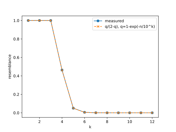
The shape is explained by occupancy. A string has \(n-k+1\approx n\) windows spread over \(10^k\) possible substrings, so a fixed substring occurs with probability about \(q_k=1-e^{-n/10^k}\), roughly independently in \(\mathbf{x}\) and \(\mathbf{y}\); hence
\begin{equation*} \text{resemblance}\approx\frac{10^kq_k^2}{10^k(2q_k-q_k^2)}=\frac{q_k}{2-q_k}, \end{equation*}
which gives \(1.000,\ 0.462,\ 0.0499,\ 0.0050,\ 0.0005\) for \(k=3,\dots,7\) (dashed curve), matching the run: \(q_k\to1\) for \(10^k\ll n\), and the resemblance is about \(n/(2\cdot10^k)\) for \(10^k\gg n\).
(Random strings, theoretical analysis.) Consider random strings of length \(n\) composed of the integers \(0\) through \(9\), where we represent a string \(\mathbf{x}\) by its set \(S_k(\mathbf{x})\) of length-\(k\) substrings. Consider now drawing two random strings \(\mathbf{x}\) and \(\mathbf{y}\) of length \(n\) and computing their resemblance \(\frac{|S_k(\mathbf{x})\cap S_k(\mathbf{y})|}{|S_k(\mathbf{x})\cup S_k(\mathbf{y})|}\).
(1) Prove that for \(k\le\frac12\log_{10}(n)\), with high probability as \(n\) goes to infinity the two strings have resemblance equal to \(1\).
(2) Prove that for \(k\ge3\log_{10}(n)\), with high probability as \(n\) goes to infinity the two strings have resemblance equal to \(0\).
(1) Whp both \(S_k(\mathbf{x})\) and \(S_k(\mathbf{y})\) equal all of \(\{0,\dots,9\}^k\), so the resemblance is \(1\). Here \(1\le k\le\frac12\log_{10}n\), so \(10^k\le\sqrt n\) and \(k\le\log_{10}n\). The \(\lfloor n/k\rfloor\) disjoint windows starting at positions \(1,k+1,2k+1,\dots\) of \(\mathbf{x}\) are independent uniform elements of \(\{0,\dots,9\}^k\), and \(\lfloor n/k\rfloor\ge n/(2k)\) once \(n\ge2k\). For a fixed \(w\in\{0,\dots,9\}^k\), using \(1-t\le e^{-t}\),
\begin{equation*} \begin{aligned} \mathrm{Prob}\bigl(w\notin S_k(\mathbf{x})\bigr) &\le(1-10^{-k})^{\lfloor n/k\rfloor}\le\exp\Bigl(-\frac{n}{2k\,10^k}\Bigr)\\ &\le\exp\Bigl(-\frac{n}{\log_{10}n\cdot\sqrt n}\Bigr)=\exp\Bigl(-\frac{\sqrt n}{\log_{10}n}\Bigr). \end{aligned} \end{equation*}
A union bound over the \(10^k\le\sqrt n\) choices of \(w\) and the two strings gives
\begin{equation*} \mathrm{Prob}\bigl(S_k(\mathbf{x})\ne\{0,\dots,9\}^k\ \text{or}\ S_k(\mathbf{y})\ne\{0,\dots,9\}^k\bigr) \le2\sqrt n\,e^{-\sqrt n/\log_{10}n}\to0, \end{equation*}
uniformly in \(k\) in the range. Off this event \(S_k(\mathbf{x})=S_k(\mathbf{y})\), so the resemblance is \(1\).
(2) Whp \(S_k(\mathbf{x})\cap S_k(\mathbf{y})=\emptyset\); the union is nonempty (assume \(k\le n\), so both strings have at least one window), so the resemblance is \(0\). Here \(10^k\ge n^3\). For any start positions \(i,j\), the window of \(\mathbf{y}\) at \(j\) is uniform on \(\{0,\dots,9\}^k\) and independent of \(\mathbf{x}\), so
\begin{equation*} \mathrm{Prob}\bigl(\mathbf{x}[i..i+k-1]=\mathbf{y}[j..j+k-1]\bigr)=10^{-k}. \end{equation*}
A common substring means some pair \((i,j)\) of the at most \(n^2\) start pairs matches, so
\begin{equation*} \mathrm{Prob}\bigl(S_k(\mathbf{x})\cap S_k(\mathbf{y})\ne\emptyset\bigr)\le n^2\,10^{-k}\le\frac{n^2}{n^3}=\frac1n\to0. \end{equation*}
Hence the resemblance is \(0\) with probability at least \(1-1/n\). \(\blacksquare\)
Exercises 6.22–6.25
Describe an approach for detecting plagiarism in term papers.
Turn each paper into a set of word shingles, estimate each paper’s containment in every source document from small min-hash sketches (Section 6.4), and hand only the pairs with high containment to a human or to an exact alignment step.
(i) Normalization. Remove formatting, punctuation and case, and stem the words, so that small cosmetic edits do not change the shingles. Then, as in Section 6.4, view the paper \(D\) as a sequence of words and let \(S(D)\) be the set of its runs of \(k\) consecutive words. Take \(k\) around \(5\) to \(8\). With a vocabulary of thousands of words, two independent texts share a given \(k\)-word run with negligible probability once \(k\) is a small multiple of the logarithm of the text length (the same calculation as Exercise 6.21). A shorter \(k\) produces chance matches on stock phrases, and a longer \(k\) is broken by every light rewording.
(ii) The right measure. A plagiarist usually copies a fragment of a source into a paper that is otherwise new, so resemblance can be small even when the copying is blatant. The quantity to test is
\begin{equation*} \text{containment}(P, Q) = \frac{|S(P)\cap S(Q)|}{|S(P)|}, \end{equation*}
the fraction of the paper \(P\) that also appears in the source \(Q\). It is asymmetric: it may be large for \(P\) in \(Q\) and small for \(Q\) in \(P\).
(iii) Scaling. Comparing every paper with every source (the web, earlier years’ papers, the other papers in the class) is impossible in full. Fix a random permutation (in practice a hash) \(\pi\) of the shingles and store only the sketch \(V(D)\), the shingles whose rank under \(\pi\) is \(0 \bmod m\). By Section 6.4, \(|V(P)\cap V(Q)|/|V(P)|\) is an unbiased estimate of the containment. The sketch \(F(D)\) of the \(s\) smallest shingles does not give this, because it estimates resemblance only. Index the sketches in an inverted table from shingle to documents. Each sampled shingle of \(P\) then retrieves the candidate sources directly, and only pairs that share several sampled shingles are scored.
(iv) Filtering and confirmation. Discard shingles found in many documents, such as stock phrases, the assignment prompt and standard citations, and discard text inside quotation marks that carries a citation. Flag the pairs whose estimated containment is above a threshold, recompute the exact \(|S(P)\cap S(Q)|\) for those pairs, and show the matching passages side by side. The final judgment is left to the instructor.
You are given a collection of one billion web pages and want to eliminate duplicates among them. Describe how you could do this.
Never compare pairs: hash exact copies into buckets, replace each page by a short min-hash sketch of its shingle set (Section 6.4), and use banded locality-sensitive hashing of the sketches so that only pages with high resemblance ever meet. Comparing all pairs is hopeless, since there are \(\binom{10^9}{2}\approx 5\times 10^{17}\) of them.
(i) Exact duplicates. Normalise each page (strip markup, collapse whitespace, lower-case), compute a 64-bit fingerprint, and sort or hash-partition by fingerprint (one MapReduce pass, \(O(n\log n)\) work). Keep one page per bucket. Among \(10^9\) pages the chance that two distinct pages share a fingerprint is at most \(\binom{10^9}{2}2^{-64}\approx 0.03\), and a byte comparison inside each bucket removes even that.
(ii) Near duplicates (mirrors, pages that differ only in ads or timestamps). As in Section 6.4, turn page \(D\) into the set \(S(D)\) of its length-\(k\) shingles (word \(k\)-grams, \(k\approx 5\)), and measure closeness by \(\mathrm{resemblance}(A,B)=|A\cap B|/|A\cup B|\). For a random permutation (in practice a random hash) \(\pi\) of the shingle universe,
\begin{equation*} \Pr\bigl[\min \pi(S(A))=\min \pi(S(B))\bigr]=\frac{|S(A)\cap S(B)|}{|S(A)\cup S(B)|}, \end{equation*}
because the minimum of \(\pi\) over \(S(A)\cup S(B)\) is equally likely to be any element of the union, and the two minima agree exactly when it falls in the intersection. With \(200\) independent hashes the sketch of a page is \(200\) numbers (800 bytes at 32 bits each, about 800 GB for the whole collection), and the fraction of agreeing coordinates estimates the resemblance with standard deviation at most \(1/\sqrt{4\cdot 200}\approx 0.035\).
(iii) Finding candidate pairs. Split the \(200\) coordinates into \(b=20\) bands of \(r=10\) and hash each band; two pages become candidates if some band matches exactly. A pair of resemblance \(s\) becomes a candidate with probability \(1-(1-s^{10})^{20}\):
| \(s\) | 0.9 | 0.8 | 0.7 | 0.5 | 0.3 |
|---|---|---|---|---|---|
| probability | 0.9998 | 0.897 | 0.436 | 0.019 | 0.0001 |
The threshold sits near \((1/20)^{1/10}\approx 0.74\), and each band costs one sort of \(10^9\) keys.
(iv) Verify and merge. For each candidate pair compute the sketch agreement (or the exact resemblance), keep the pairs above a threshold such as \(0.9\), join them with union-find, and keep one representative per connected component (for instance the oldest or most-linked URL).
The book prints the lyric of the song You’ll Never Walk Alone (Rodgers and Hammerstein, Carousel, 1945). Read it as a single string of 359 symbols over a 27-symbol alphabet (case-sensitive letters, comma, period, apostrophe and blank), with every line break read as one blank. How large must \(k\) be for the lyric to be uniquely recoverable from the set of all its length-\(k\) shingles (contiguous substrings of \(k\) symbols, Section 6.4)? Treat the blank as a symbol.
\(k=26\): two more than the length \(L=24\) of the longest window that occurs twice, so that every window of length \(k-1=25\) is unique.
Let \(s\) have length \(n\), let \(S_k\) be its set of length-\(k\) shingles, and let \(G_k\) be the graph whose vertices are the length-\((k-1)\) strings and whose edges are the shingles \(w\in S_k\), each joining its prefix to its suffix. The string \(s\) is a walk in \(G_k\) that uses every edge.
(i) If the \(n-k+2\) windows \(s[i,i+k-1)\) of length \(k-1\) are pairwise distinct, then \(G_k\) is a simple path. Every string \(t\) with shingle set \(S_k\) is a walk using every edge, so it starts at the unique vertex of in-degree \(0\) and follows the path; hence \(t=s\).
(ii) If some length-\((k-1)\) window occurs at positions \(i<j\), the walk revisits that vertex, so \(s[i,j)\) is a cycle in \(G_k\). Then
\begin{equation*} t=s[0,j)\,s[i,n) \end{equation*}
traverses the cycle twice: \(t\neq s\) has the same shingle set \(S_k\).
So \(s\) is recoverable exactly when all length-\((k-1)\) windows are distinct, that is when \(k-1>L\), with \(L\) the length of the longest substring occurring at least twice. Here the longest repeat is the 24-symbol window " you’ll never walk alone" (leading blank included), which ends both of the closing phrases; every repeat in the “walk on” lines is shorter. Hence \(L=24\) and the threshold is \(k=L+2=26\). Lower-casing the text first does not change \(L\), so the answer is the same if case is ignored. (Check! A python scan of all windows confirms that the 25-symbol windows are distinct while two 24-symbol windows coincide, and that at \(k=25\) the spliced string of (ii) has the same shingle set.)
(Blast.) A long string \(A\) (length about \(10^9\)) and a shorter string \(B\) (length about \(10^5\)) are given. We want a position in \(A\) at which a substring \(B^{\prime}\) close to \(B\) begins. Dynamic programming solves this in polynomial time; give a faster algorithm. Hint (shingling): fix a small length, say \(7\), and compare the length-\(7\) shingles of \(A\) and \(B\). If a close approximation of \(B\) is a substring of \(A\), many shingles of \(B\) must also be shingles of \(A\), which locates the approximate position of the match; a final step can then find the best match.
Seed with shingles, vote by diagonal, then run the DP only on the few windows that win the vote. Write \(n=|A|\), \(m=|B|\), alphabet size \(\sigma\), shingle length \(k\) (as in Section 6.4), and target edit distance \(e\) (insertions, deletions, substitutions). Full semi-global DP costs \(\Theta(nm)=10^{14}\).
1. Put every k-shingle B[j..j+k) in a hash table T (value: list of j).
2. Slide a rolling (Karp-Rabin) hash over A; for each position i
   and each j in T[A[i..i+k)] with equal strings, record a hit on
   diagonal d = i - j:  count[floor(d / W)] += 1,  where W = 2e+1.
3. Candidates: buckets b with count[b] + count[b+1] >= tau,
   tau = m - k + 1 - k*e.
4. For each candidate b run semi-global edit-distance DP of B
   against the window A[bW .. (b+2)W + m + e); return the best
   start position found over all candidates.
Correctness. Let \(B^{\prime}=A[p..p+L)\) with \(\mathrm{ed}(B,B^{\prime})\le e\) and fix an optimal alignment. Each edit operation at position \(t\) of \(B\) touches only the shingles starting in \([t-k+1,t]\), so at most \(k\) shingles; every other shingle \(B[j..j+k)\) is copied verbatim into \(A\) at position \(i=p+(\#\text{ins}-\#\text{del before } j)\). Hence
\begin{equation*} \begin{aligned} \#\{\text{hits with } d\in[p-e,p+e]\} &\ge (m-k+1)-ke=\tau , \end{aligned} \end{equation*}
and an interval of \(2e+1=W\) consecutive diagonals meets at most two adjacent buckets, so the bucket pair containing it passes step 3. Since \(p\in[bW,(b+2)W)\) and \(L\le m+e\), \(B^{\prime}\) lies inside the step-4 window, and the DP finds a match at least as good as \(B^{\prime}\). Thus every match within distance \(e\) (in particular the best one, if its distance is \(\le e\)) is found deterministically; this needs \(\tau>0\), i.e. \(e<(m-k+1)/k\), about \(14\%\) errors for \(k=7\) (use smaller \(k\) for noisier matches).
Running time. Steps 1-2 cost \(O(n+m+H)\), \(H\) the number of hits. In the random model (independent uniform letters), two fixed shingles agree with probability \(\sigma^{-k}\); take \(\sigma=26\), \(k=7\) and \(e=10^4\) (\(10\%\) errors), so \(W=20001\) and \(\tau=29994\). Then
\begin{equation*} \begin{aligned} \mathbb{E}H &\le m+\frac{nm}{\sigma^{k}} \approx 10^{5}+\frac{10^{14}}{26^{7}}\approx 1.1\times10^{5},\\ \mathbb{E}\,(\text{false hits per bucket pair}) &\le \frac{2Wm}{\sigma^{k}}\approx 0.50, \end{aligned} \end{equation*}
and by Markov’s inequality and linearity over the \(n/W\approx 5\times10^4\) bucket pairs,
\begin{equation*} \begin{aligned} \mathbb{E}\,\#\{\text{false candidates}\} &\le \frac{n}{W}\cdot\frac{2Wm\,\sigma^{-k}}{\tau} =\frac{2nm}{\sigma^{k}\tau}\approx 0.83 . \end{aligned} \end{equation*}
(This is why \(k\approx\log_\sigma n\): then \(\sigma^{k}\gtrsim n\).) The true match passes in at most \(3\) bucket pairs (those meeting buckets \(b,b+1\)), so the expected number of DPs is below \(4\), each costing \(O(m(m+2W+e))\approx1.5\times10^{10}\) cell updates; the expected total is
\begin{equation*} \boxed{\;O\!\Big(n+\frac{nm}{\sigma^{k}}+m(m+e)\Big) \approx 6\times10^{10}\ \ll\ nm=10^{14},\;} \end{equation*}
with the best match within distance \(e\) guaranteed.
Clustering
Exercises 7.1–7.7
Construct examples where using distances instead of distance squared gives bad results for Gaussian densities. For example, pick samples from two 1-dimensional unit variance Gaussians, with their centers 10 units apart. Cluster these samples by trial and error into two clusters, first according to \(k\)-means and then according to the \(k\)-median criteria. The \(k\)-means clustering should essentially yield the centers of the Gaussians as cluster centers. What cluster centers do you get when you use the \(k\)-median criterion?
For two equal-weight Gaussians the \(k\)-median centers are the two cluster medians, which also sit near the true centers but are noisier estimates. Give the Gaussians unequal weights and \(k\)-median breaks down: it splits the big Gaussian in two and lumps the small one in with a piece of it.
Since the clusters on a line are contiguous (Section 7.2.5), “trial and error” can be done exhaustively: try every split point of the sorted sample, give each side its optimal center (the mean for \(k\)-means by Corollary 7.2, the median for \(k\)-median by Exercise 7.3), and keep the cheapest split.
import numpy as np
def best(x, kind):                       # exhaustive 2-clustering on the line
    x = np.sort(x); out = None
    for s in range(1, len(x)):
        L, R = x[:s], x[s:]
        if kind == 'mean':
            c = (L.mean(), R.mean()); f = lambda v, m: ((v - m)**2).sum()
        else:
            c = (np.median(L), np.median(R)); f = lambda v, m: abs(v - m).sum()
        cost = f(L, c[0]) + f(R, c[1])
        if out is None or cost < out[0]: out = (cost, c, s)
    return out
rng = np.random.default_rng(0)
x = np.r_[rng.normal(0, 1, 100), rng.normal(10, 1, 100)]
print(best(x, 'mean'), best(x, 'med'))
rng = np.random.default_rng(1)
y = np.r_[rng.normal(0, 1, 1000), rng.normal(10, 1, 10)]
print(best(y, 'mean'), best(y, 'med'))
(i) Equal weights, 100 points from each of \(N(0,1)\) and \(N(10,1)\): both criteria split the sample into the two Gaussians. The \(k\)-means centers are \((0.081,\,9.949)\) and the \(k\)-median centers are \((0.073,\,9.987)\). Over 2000 repetitions the mean squared center error was \(0.0101\) for \(k\)-means and \(0.0160\) for \(k\)-median. Their ratio is \(0.633\approx 2/\pi\), the asymptotic efficiency of the sample median relative to the sample mean for a Gaussian. Section 7.2.1 says the \(k\)-means centers are the maximum-likelihood estimates, so \(k\)-median is strictly worse here.
(ii) Unequal weights, 1000 points from \(N(0,1)\) and 10 points from \(N(10,1)\):
| criterion | split | centers | cost (natural split) | cost (found split) |
|---|---|---|---|---|
| \(k\)-means | 1000 / 10 | \(-0.05,\ 9.90\) | 986.9 | 986.9 |
| \(k\)-median | 494 / 516 | \(-0.72,\ 0.63\) | 791.9 | 559.1 |
Under \(k\)-median the ten far points cost only about \(10\cdot 10=100\) in total when they join the right half of the big Gaussian. Splitting \(N(0,1)\) at its median saves far more than that: the cost per point falls from \(\mathbb{E}|X|=\sqrt{2/\pi}\approx 0.80\) to about \(0.47\) (the half-normal’s mean absolute deviation about its median), a saving of about 325. Under \(k\)-means the same ten points would cost about \(10\cdot 10^2=1000\), which is more than the split saves: the cost per point falls from \(1\) to \(1-2/\pi\approx 0.36\), a saving of about 637. So \(k\)-means keeps the true clusters and \(k\)-median does not. The same happened with 20 far points; with 40 far points \(k\)-median recovers the true clusters again.
Let \(v=(1,3)\). What is the \(L_1\) norm of \(v\)? The \(L_2\) norm? The square of the \(L_1\) norm?
\begin{equation*} |v|_1=|1|+|3|=4,\qquad |v|_2=\sqrt{1^2+3^2}=\sqrt{10},\qquad |v|_1^2=16. \end{equation*}
Show that in 1-dimension, the center of a cluster that minimizes the sum of distances of data points to the center is in general not unique. Suppose we now require the center also to be a data point; then show that it is the median element (not the mean). Further in 1-dimension, show that if the center minimizes the sum of squared distances to the data points, then it is unique.
The minimizers of \(f(x)=\sum_i|a_i-x|\) are the medians of the sorted data \(a_{(1)}\le\cdots\le a_{(n)}\), a whole interval when \(n\) is even. Indeed \(f\) is convex and piecewise linear, and wherever \(x\) is not a data point its slope is
\begin{equation*} f^{\prime}(x)=\#\{i: a_i<x\}-\#\{i: a_i>x\}, \end{equation*}
which is negative for \(x<a_{(\lceil n/2\rceil)}\) and positive for \(x>a_{(\lfloor n/2\rfloor+1)}\).
(i) Non-uniqueness. If \(n=2m\), the slope is \(m-m=0\) on \((a_{(m)},a_{(m+1)})\), so every point of \([a_{(m)},a_{(m+1)}]\) minimizes \(f\). For example, with data \(\{0,1\}\) we get \(f(x)=1\) for every \(x\in[0,1]\). (If \(n=2m+1\), the minimizer is the unique point \(a_{(m+1)}\).)
(ii) Data-point centers. \(f\) decreases up to \(a_{(\lceil n/2\rceil)}\), increases from \(a_{(\lfloor n/2\rfloor+1)}\) on, and is constant between them. So among the data points the minimizers are exactly the median elements: \(a_{(m+1)}\) when \(n=2m+1\), and \(a_{(m)}\) or \(a_{(m+1)}\) when \(n=2m\). The mean need not even be a candidate. For \(\{0,0,3\}\) the mean \(1\) is not a data point, and \(f(0)=3<f(3)=6\), so the optimal center is the median \(0\).
(iii) Squared distances. With \(c=\frac1n\sum_i a_i\), Lemma 7.1 gives
\begin{equation*} \sum_i(a_i-x)^2=\sum_i(a_i-c)^2+n(x-c)^2, \end{equation*}
which is strictly larger than its value at \(x=c\) for every \(x\ne c\). So the minimizer \(x=c\) is unique.
Construct a block diagonal matrix \(A\) with three blocks of size 50. Each matrix element in a block has value \(p=0.7\) and each matrix element not in a block has value \(q=0.3\). Generate a \(150\times 150\) matrix \(B\) of random numbers in the range \([0,1]\). If \(b_{ij}\ge a_{ij}\) replace \(a_{ij}\) with the value one. Otherwise replace \(a_{ij}\) with value zero. The rows of \(A\) have three natural clusters. Generate a random permutation and use it to permute the rows and columns of the matrix \(A\) so that the rows and columns of each cluster are randomly distributed. (1) Apply the \(k\)-means algorithm to \(A\) with \(k=3\). Do you find the correct clusters? (2) Apply the \(k\)-means algorithm to \(A\) for \(1\le k\le 10\). Plot the value of the sum of squares to the cluster centers versus \(k\). Was three the correct value for \(k\)?
(1) Yes: \(k\)-means with \(k=3\) recovered the three planted clusters exactly (adjusted Rand index \(1.0\)). (2) Yes: the curve has a sharp elbow at \(k=3\).
The printed rule \(b_{ij}\ge a_{ij}\) makes in-block entries one with probability \(1-p=0.3\), so I use the intended \(b_{ij}\le a_{ij}\) (the printed rule gives the complement \(1-A\), and the same clusters).
import numpy as np, matplotlib.pyplot as plt
from sklearn.cluster import KMeans
from sklearn.metrics import adjusted_rand_score
rng = np.random.default_rng(0)
lab = np.repeat([0, 1, 2], 50)
P = np.where(lab[:, None] == lab[None, :], 0.7, 0.3)
A = (rng.random((150, 150)) <= P).astype(float)
pi = rng.permutation(150); A = A[pi][:, pi]; lab = lab[pi]
km = KMeans(3, n_init=10, random_state=0).fit(A)
print(adjusted_rand_score(lab, km.labels_))
ks = range(1, 11)
sse = [KMeans(k, n_init=10, random_state=0).fit(A).inertia_ for k in ks]
plt.plot(ks, sse, 'o-'); plt.xlabel('k'); plt.ylabel('sum of squares')
plt.savefig('fds-ch07-blockelbow.svg')
The sum of squared distances to the cluster centers was:
| \(k\) | 1 | 2 | 3 | 4 | 5 | 6 | 7 | 8 | 9 | 10 |
|---|---|---|---|---|---|---|---|---|---|---|
| SSE | 5476.2 | 5006.6 | 4584.9 | 4533.2 | 4490.3 | 4446.2 | 4397.2 | 4361.5 | 4318.5 | 4273.4 |
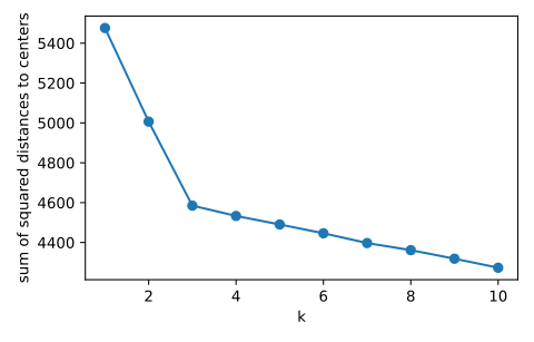
Going from \(k=1\) to \(k=3\) removes about 470 and 422. After that each extra center removes only 36 to 52, because it just fits noise. By Lemma 7.1 the model predicts this:
- With the three true clusters, the cost is pure Bernoulli noise: \(150^2\cdot p(1-p)(1-\tfrac1{50})\approx 4630\).
- With one cluster, the noise is \(150^2\cdot 0.21\,(1-\tfrac1{150})\approx 4694\), and each row also pays \(50(0.7-\tfrac{13}{30})^2+100(0.3-\tfrac{13}{30})^2\approx 5.33\) to the overall mean, about 800 in all, for a total near 5490.
Let \(M\) be a \(k\times k\) matrix whose elements are numbers in the range \([0,1]\). A matrix entry close to one indicates that the row and column of the entry correspond to closely related items and an entry close to zero indicates unrelated entities. Develop an algorithm to match each row with a closely related column where a column can be matched with only one row.
Pose it as a maximum-weight perfect matching in the complete bipartite graph between rows and columns, where edge \((i,j)\) has weight \(m_{ij}\). That is, find a permutation \(\sigma\) that solves
\begin{equation*} \max_{\sigma\in S_k}\ \sum_{i=1}^k m_{i\sigma(i)}. \end{equation*}
This is the assignment problem. The Hungarian (Kuhn-Munkres) algorithm, run on costs \(1-m_{ij}\), solves it exactly in \(O(k^3)\) time.
Method (2): if “closely related” should hold for every matched pair, not just on average, maximize the worst matched entry \(\min_i m_{i\sigma(i)}\) instead. That needs only augmenting paths:
sort the distinct entries of M:  t_1 > t_2 > ... > t_s
binary search for the largest threshold t = t_j such that
    G_t = { (i,c) : M[i][c] >= t }  has a perfect matching
perfect-matching test (Kuhn's augmenting paths):
    match[c] = none for every column c
    for each row i:
        clear visited; if not TRY(i) then return FAIL
    return match
TRY(i):
    for each column c with (i,c) in G_t and c not visited:
        mark c visited
        if match[c] = none or TRY(match[c]):
            match[c] = i; return TRUE
    return FALSE
(i) Binary search is valid: raising \(t\) only deletes edges, so the property “\(G_t\) has a perfect matching” is monotone in \(t\). At \(t=t_s\) the graph is complete, so a perfect matching exists.
(ii) The matching test is correct: by Berge’s theorem a matching is maximum if and only if it has no augmenting path, and TRY searches for exactly such a path from each row.
(iii) Running time: each test costs \(O(k\cdot k^2)\), and there are \(O(\log k^2)\) thresholds to try, so the total is \(O(k^3\log k)\). The matching returned at the optimal threshold pairs every row with a distinct column, and every matched entry is at least \(t^\ast\), the largest value for which that is possible.
The simple greedy algorithm of Section 7.3 assumes that we know the clustering radius \(r\). Suppose we do not. Describe how we might arrive at the correct \(r\)?
Run farthest traversal itself and read \(r\) off its output. Let \(c_1,\dots,c_k\) be the centers it picks, and let
\begin{equation*} R=\max_x d(x,\{c_1,\dots,c_k\}), \end{equation*}
attained at some point \(x^\ast\). Then \(R/2\le \mathrm{OPT}\le R\), where \(\mathrm{OPT}\) is the optimal \(k\)-center radius. The upper bound holds because the traversal produces a \(k\)-clustering of radius \(R\). For the lower bound, consider the step at which \(c_t\) was chosen. The distance from \(x^\ast\) to the current centers at that step is at least its final value \(R\), and \(c_t\) was the farthest point, so \(d(c_t,\{c_1,\dots,c_{t-1}\})\ge R\). Therefore the \(k+1\) points \(c_1,\dots,c_k,x^\ast\) are pairwise at distance at least \(R\). Two of them lie in the same cluster of an optimal clustering, so by the triangle inequality \(R\le 2\,\mathrm{OPT}\). This is the argument of Theorem 7.3, and no value of \(r\) is needed as input.
Method (2): search over \(r\). Suppose instead the greedy procedure is the threshold version: repeatedly make an uncovered point a center and cover every point within \(2r\) of it, and call the run a success if it uses at most \(k\) centers. Let \(\mathrm{OPT}_D\) be the optimal radius when the centers must be data points. Then:
(i) The run succeeds for every \(r\ge \mathrm{OPT}_D\). Its centers are pairwise more than \(2r\) apart, and each optimal ball of radius \(\mathrm{OPT}_D\le r\) has diameter at most \(2r\), so each such ball contains at most one center.
(ii) \(\mathrm{OPT}_D\) belongs to the finite candidate set \(D=\{0\}\cup\{d(x,y): x,y \text{ data points}\}\).
Sort \(D\) and binary search for adjacent candidates \(r^{\prime}<\hat r\) such that the run at \(r^{\prime}\) fails and the run at \(\hat r\) succeeds. (The largest distance always succeeds; if \(0\) also succeeds, take \(\hat r=0\).) By (i), failure at \(r^{\prime}\) means \(r^{\prime}<\mathrm{OPT}_D\). By (ii), \(\mathrm{OPT}_D\in D\) and \(\mathrm{OPT}_D>r^{\prime}\), so \(\hat r\le \mathrm{OPT}_D\). Hence \(O(\log n)\) greedy runs give a \(k\)-clustering of radius
\begin{equation*} 2\hat r\le 2\,\mathrm{OPT}_D\le 4\,\mathrm{OPT}, \end{equation*}
where \(\mathrm{OPT}_D\le 2\,\mathrm{OPT}\) is the \(k\)-center version of Exercise 7.7. (Moving each center to a point of its own cluster at most doubles every radius, by the triangle inequality.)
For the \(k\)-median problem, show that there is at most a factor of two ratio between the optimal value when we either require all cluster centers to be data points or allow arbitrary points to be centers.
Move each optimal center to the data point of its cluster that is nearest to it. This at most doubles the cost.
Let \(\mathrm{OPT}\) be the optimal value with arbitrary centers, achieved by clusters \(C_1,\dots,C_k\) with centers \(c_1,\dots,c_k\), and let \(\mathrm{OPT}_D\) be the optimal value with data-point centers. Since data-point centers are a special case of arbitrary centers, \(\mathrm{OPT}\le\mathrm{OPT}_D\). For each \(j\) pick \(a_j^\ast\in C_j\) minimizing \(d(a,c_j)\) over \(a\in C_j\). The triangle inequality then gives
\begin{equation*} \begin{aligned} \sum_{a\in C_j} d(a,a_j^\ast) &\le \sum_{a\in C_j}\bigl(d(a,c_j)+d(c_j,a_j^\ast)\bigr)\\ &\le \sum_{a\in C_j}\bigl(d(a,c_j)+d(c_j,a)\bigr) =2\sum_{a\in C_j} d(a,c_j). \end{aligned} \end{equation*}
Summing over \(j\) shows that the data-point centers \(a_1^\ast,\dots,a_k^\ast\) with the same clusters cost at most \(2\,\mathrm{OPT}\). Reassigning each point to its nearest center can only lower the cost further. Hence
\begin{equation*} \mathrm{OPT}\le \mathrm{OPT}_D\le 2\,\mathrm{OPT}. \end{equation*}
Exercises 7.8–7.14
For the \(k\)-means problem, show that there is at most a factor of four ratio between the optimal value when we either require all cluster centers to be data points or allow arbitrary points to be centers.
The ratio is in fact at most \(2\), hence at most \(4\). Let \(\mathrm{OPT}\) be the optimum with arbitrary centers and \(\mathrm{OPT}_{D}\) the optimum with data-point centers; trivially \(\mathrm{OPT}\le\mathrm{OPT}_D\). Take an optimal unrestricted clustering \(C_1,\dots,C_k\) (nonempty clusters, \(|C_j|=n_j\)); by Corollary 7.2 its centers are the centroids \(c_j\). In each \(C_j\) pick the data point \(a^{(j)}\in C_j\) nearest to \(c_j\), so \(|a^{(j)}-c_j|^2\le\frac1{n_j}\sum_{a_i\in C_j}|a_i-c_j|^2\). By Lemma 7.1,
\begin{equation*} \begin{aligned} \sum_{a_i\in C_j}|a_i-a^{(j)}|^2 &=\sum_{a_i\in C_j}|a_i-c_j|^2+n_j\,|c_j-a^{(j)}|^2\\ &\le 2\sum_{a_i\in C_j}|a_i-c_j|^2 . \end{aligned} \end{equation*}
Summing over \(j\), the clustering \(C_1,\dots,C_k\) with data-point centers \(a^{(1)},\dots,a^{(k)}\) costs at most \(2\,\mathrm{OPT}\), so
\begin{equation*} \mathrm{OPT}\le\mathrm{OPT}_D\le 2\,\mathrm{OPT}\le 4\,\mathrm{OPT}. \end{equation*}
Consider clustering points in the plane according to the \(k\)-median criterion, where cluster centers are required to be data points. Enumerate all possible clusterings and select the one with the minimum cost. The number of possible ways of labeling \(n\) points, each with a label from \(\{1,2,\dots,k\}\) is \(k^n\) which is prohibitive. Show that we can find the optimal clustering in time at most a constant times \(\binom{n}{k}+k^2\). Note that \(\binom{n}{k}\le n^k\) which is much smaller than \(k^n\) when \(k\ll n\).
Enumerate the \(\binom nk\) possible center sets instead of the \(k^n\) labelings: this finds the optimum in time \(O\bigl(nk\binom nk\bigr)=O(kn^{k+1})\). (The printed bound \(\binom nk+k^2\) omits the \(O(nk)\) cost of scoring each candidate center set; we prove the intended bound \(O(nk\binom nk)\), i.e. a constant times \(\binom nk\) candidates.)
For a set \(S\) of \(k\) data points put
\begin{equation*} \mathrm{cost}(S)=\sum_{i=1}^n\min_{c\in S}d(a_i,c). \end{equation*}
(i) For a fixed center set \(S\), assigning every point to its nearest center minimizes \(\Phi_{\mathrm{kmedian}}\) term by term, so the best clustering with centers \(S\) costs exactly \(\mathrm{cost}(S)\).
(ii) An optimal clustering uses at most \(k\) distinct data points as centers; padding with further data points (which can only lower \(\mathrm{cost}\)) gives a \(k\)-set \(S^\ast\) with \(\mathrm{cost}(S^\ast)=\mathrm{OPT}\).
Hence
\begin{equation*} \mathrm{OPT}=\min_{S\subseteq\{a_1,\dots,a_n\},\ |S|=k}\mathrm{cost}(S), \end{equation*}
and the minimizing \(S\) with its nearest-center assignment is an optimal clustering. Listing the \(k\)-subsets in lexicographic order costs \(O(k)\) each, and evaluating \(\mathrm{cost}(S)\) costs \(nk\) distance computations and comparisons, for a total of
\begin{equation*} O\Bigl(nk\binom nk\Bigr)\le O\bigl(kn^{k+1}\bigr). \end{equation*}
Suppose in the previous exercise, we allow any point in space (not necessarily data points) to be cluster centers. Show that the optimal clustering may be found in time at most a constant times \(n^{2k^2}\).
Enumerate Voronoi-type partitions: every pair of optimal clusters is cut off from each other by a line, and a line splits \(n\) points in at most \(3n^3\) ways, so there are at most \(O\bigl(n^{3\binom k2}\bigr)\) candidate clusterings. Throughout, computing the optimal center of one cluster (its Fermat-Weber point for \(k\)-median, its centroid for \(k\)-means) is counted as an \(O(n)\) primitive, as the operation count of the exercise intends; \(k\) is fixed and \(k\ge2\) (for \(k=1\) there is one clustering).
(i) Structure. Let \(c_1,\dots,c_k\) be optimal centers and assign each point to its nearest center, ties to the smallest index; this does not change the cost. For \(j<l\) let \(L_{jl}\) be the perpendicular bisector of \(c_jc_l\). Then \(C_j\) lies in the closed side of \(L_{jl}\) containing \(c_j\) and \(C_l\) in the open side containing \(c_l\), so moving \(L_{jl}\) slightly toward \(c_l\) gives a line \(\ell_{jl}\) through no data point with \(C_j\) and \(C_l\) on opposite sides (if \(c_j=c_l\) then \(C_l=\emptyset\) and a line with all of \(P\) on one side will do).
(ii) Few line-splits. If a line through no data point splits the point set \(P\) into \((U,P\setminus U)\) with both parts nonempty, translate it until it meets a data point and rotate it about that point until it meets a second one (if all points are collinear, use their common line). The resulting line \(\ell\) through data points \(p,q\) has \(U\) and \(P\setminus U\) in its opposite closed sides, and on \(\ell\) the two parts are separated by a single cut point (the original line meets \(\ell\) at most once). Hence a split is determined by the pair \((p,q)\), a cut among at most \(n+1\) positions on \(\ell\), which closed side of \(\ell\) holds \(U\), and which side of the cut holds \(U\cap\ell\); adding the two trivial splits,
\begin{equation*} \#\{\text{line splits of }P\}\le 4\binom n2(n+1)+2\le 3n^3, \end{equation*}
and they can all be listed in \(O(n^4)\) time.
(iii) Algorithm. For every choice of one split \((U_{jl},P\setminus U_{jl})\) for each pair \(j<l\), put
\begin{equation*} D_j=\{a\in P:\ a\in U_{jl}\ \forall l>j,\ a\notin U_{lj}\ \forall l<j\}. \end{equation*}
The \(D_j\) are pairwise disjoint (a point of \(D_j\cap D_l\), \(j<l\), would be both in and out of \(U_{jl}\)). Keep the choice when they cover \(P\), compute the optimal center of each \(D_j\) and the cost, and return the cheapest. Choosing \(U_{jl}\) as the \(c_j\)-side of \(\ell_{jl}\) from (i) gives \(C_j\subseteq D_j\) for every \(j\), hence \(D_j=C_j\); so the optimum is among the candidates.
(iv) Time. Each candidate costs \(O(k^2n)\) to form plus \(k\) center primitives of total cost \(O(n)\), so the total is
\begin{equation*} \begin{aligned} O(n^4)+O\bigl((3n^3)^{\binom k2}\,k^2n\bigr) &=O\bigl(n^{\frac32k(k-1)+1}+n^4\bigr)\\ &\le O\bigl(n^{2k^2}\bigr), \end{aligned} \end{equation*}
because \(2k^2-\tfrac32k(k-1)-1=\tfrac12(k^2+3k-2)\ge0\) and \(2k^2\ge8\) for \(k\ge2\).
Corollary 7.2 shows that for a set of points \(\{a_1,a_2,\dots,a_n\}\), there is a unique point \(x\), namely their centroid, which minimizes \(\sum_{i=1}^n|a_i-x|^2\). Show examples where the \(x\) minimizing \(\sum_{i=1}^n|a_i-x|\) is not unique. (Consider just points on the real line.) Show examples where the \(x\) defined as above are far apart from each other.
Take \(\{0,M\}\) with \(M>0\): every \(x\in[0,M]\) minimizes, since
\begin{equation*} f(x)=|x|+|M-x|= \begin{cases} M, & 0\le x\le M,\\ M+2\,\mathrm{dist}(x,[0,M]), & \text{otherwise}. \end{cases} \end{equation*}
So the minimizer of \(\sum_i|a_i-x|\) is not unique, and two minimizers (\(0\) and \(M\)) are \(M\) apart, arbitrarily far.
For the minimizers of the two criteria, take \(\{0,0,M\}\). Then \(g(x)=2|x|+|M-x|\) has slope \(-3\) on \((-\infty,0)\), \(+1\) on \((0,M)\) and \(+3\) on \((M,\infty)\), so its unique minimizer is the median \(x=0\), while the minimizer of \(\sum_i|a_i-x|^2\) is the centroid \(M/3\); they are
\begin{equation*} \Bigl|0-\frac M3\Bigr|=\frac M3\xrightarrow[M\to\infty]{}\infty \end{equation*}
apart.
Let \(\{\mathbf a_1,\mathbf a_2,\dots,\mathbf a_n\}\) be a set of unit vectors in a cluster. Let \(\mathbf c=\frac1n\sum_{i=1}^n\mathbf a_i\) be the cluster centroid. The centroid \(\mathbf c\) is not in general a unit vector. Define the similarity between two points \(\mathbf a_i\) and \(\mathbf a_j\) as their dot product. Show that the average cluster similarity \(\frac1{n^2}\sum_{i,j}\mathbf a_i\mathbf a_j^T\) is the same whether it is computed by averaging all pairs or computing the average similarity of each point with the centroid of the cluster.
Both equal \(|\mathbf c|^2\). (Reading the \(\mathbf a_i\) as row vectors, \(\mathbf a_i\mathbf a_j^T=\mathbf a_i\cdot\mathbf a_j\) is the dot product.) By bilinearity,
\begin{equation*} \begin{aligned} \frac1{n^2}\sum_{i,j}\mathbf a_i\cdot\mathbf a_j &=\Bigl(\frac1n\sum_i\mathbf a_i\Bigr)\cdot\Bigl(\frac1n\sum_j\mathbf a_j\Bigr)\\ &=\mathbf c\cdot\mathbf c,\\ \frac1n\sum_i\mathbf a_i\cdot\mathbf c &=\Bigl(\frac1n\sum_i\mathbf a_i\Bigr)\cdot\mathbf c=\mathbf c\cdot\mathbf c . \end{aligned} \end{equation*}
For some synthetic data estimate the number of local minima for \(k\)-means by using the birthday estimate. Is your estimate an unbiased estimate of the number? an upper bound? a lower bound? Why?
The birthday estimate is not unbiased: it estimates \(1/\sum_i p_i^2\), which is at most the number of local minima, so it is (up to small-sample noise) a lower bound, and on our data a severe one: \(207\), while \(2882\) distinct minima were actually observed.
Data: \(n=100\) points in the plane, \(20\) from each of five unit-variance Gaussians centred at \((0,0),(6,0),(0,6),(6,6),(3,3)\), clustered with \(k=7\). Each run starts Lloyd’s algorithm (Section 7.2.3) at \(7\) random data points and runs it to a fixed point; the final partition, with labels canonicalised, identifies the local minimum.
import numpy as np
from collections import Counter
rng = np.random.default_rng(0)
X = np.vstack([rng.normal(m, 1.0, (20, 2)) for m in [(0,0),(6,0),(0,6),(6,6),(3,3)]])
k = 7
def lloyd():                      # random data-point start, run to a fixed point
    C, lab = X[rng.choice(len(X), k, replace=False)], None
    while True:
        new = ((X[:, None] - C[None]) ** 2).sum(2).argmin(1)
        if lab is not None and (new == lab).all(): break
        lab = new
        C = np.array([X[lab == j].mean(0) if (lab == j).any() else C[j] for j in range(k)])
    first = {}                    # canonical labels identify the local minimum
    return tuple(first.setdefault(l, len(first)) for l in lab)
R = [lloyd() for _ in range(1000)]
cnt = Counter(R)
coll = sum(c * (c - 1) // 2 for c in cnt.values())
print(len(cnt), coll, 1000 * 999 / 2 / coll)        # distinct, collisions, birthday estimate
R += [lloyd() for _ in range(19000)]
cnt = Counter(R)
p = np.array(list(cnt.values())) / len(R)
print(len(cnt), sum(c == 1 for c in cnt.values()), 1 / (p ** 2).sum())
If each of \(N\) minima were reached with probability \(1/N\), the number \(C\) of pairs of runs (out of \(m\)) ending at the same minimum would have \(\mathbb E\,C=\binom m2/N\), giving the birthday estimate \(\hat N=\binom m2/C\). With \(m=1000\) runs we got \(512\) distinct minima and \(C=2418\) colliding pairs, so
\begin{equation*} \hat N=\frac{\binom{1000}{2}}{2418}=\frac{499500}{2418}\approx 207 . \end{equation*}
Extending to \(20000\) runs produced \(2882\) distinct minima, \(1178\) of them seen only once (so many more remain unseen), and the empirical value of \(1/\sum_i p_i^2\) was \(\approx218\).
Why. If run \(r\) lands on minimum \(i\) with probability \(p_i\) (the size of its basin under the random start), then exactly
\begin{equation*} \mathbb E\,C=\binom m2\sum_i p_i^2, \qquad \sum_i p_i^2\ \ge\ \frac{\bigl(\sum_i p_i\bigr)^2}{N_+}=\frac1{N_+} \end{equation*}
by Cauchy-Schwarz, where \(N_+\le N\) counts the minima with \(p_i>0\); equality holds only for equal basins. So \(\hat N\) concentrates around \(1/\sum_ip_i^2\le N_+\le N\): unequal basins (a few large ones collect most collisions) and minima that the initialisation never reaches both push it down. The only upward effect is the Jensen bias \(\mathbb E[1/C]\ge1/\mathbb E[C]\), negligible once \(C\) is in the thousands. Hence the birthday estimate is a lower bound in practice, neither unbiased nor an upper bound.
Examine the example in Figure 7.9 and discuss how to fix it. Optimizing according to the \(k\)-center or \(k\)-median criteria would seem to produce clustering B while clustering A seems more desirable.
(Figure 7.9: on the left a small, tight group of about seven points; to its right, after a clear gap, a larger and more spread-out group of about twenty points. Clustering A (\(k=2\)) is the solid vertical line in the gap, separating the two groups; clustering B is a dashed vertical line through the middle of the large group, so the small group is clustered with the left half of the large group.)
Fix it by clustering on separation rather than spread: single linkage (Section 7.7.1), or any method that cuts a sparse region of a neighbourhood graph (Sections 7.5, 7.9), returns A, because the gap between the groups is wider than every gap inside the large group.
Why the center criteria fail. \(\Phi_{\mathrm{kcenter}}\) and \(\Phi_{\mathrm{kmedian}}\) (Section 7.1.2) charge each cluster for its spread and never reward a gap. If the large group has half-width \(W\) and the gap is \(s<W\), then for \(k\)-center A pays about \(W\) (one center for the whole large group), while B pays about \(\max\bigl(\tfrac{s+W}2,\tfrac W2\bigr)<W\); for \(k\)-median, B halves the distances of the twenty large-group points at the price of moving only the seven small-group points, which wins when the small group has few points. The criteria, like the equal-variance Gaussian model of Section 7.2.1 behind them, implicitly assume clusters of similar scale.
A concrete check: \(7\) points \(N(0,0.1^2 I)\) at the origin and \(20\) points uniform on \([1.2,7.2]\times[-0.6,0.6]\) (seed \(1\)), \(k=2\), centers restricted to data points.
| criterion | optimum | value of A |
|---|---|---|
| \(k\)-center | \(2.00\) (B-type: small group plus part of the large one) | \(2.65\) |
| \(k\)-median | \(29.34\) (B-type: small group plus two large-group points) | \(29.83\) |
The smallest distance from the small group to the large one is \(1.83\), while the large group stays connected through steps of length at most \(1.11\) (its longest minimum-spanning-tree edge); single linkage stopped at two clusters, and spectral clustering on the \(3\)- to \(6\)-nearest-neighbour graph, both return exactly A.
Fixes, each removing the equal-scale assumption: (i) Single linkage or a threshold graph: join points within distance \(r\) for any \(r\in(1.11,1.83)\) here and take connected components; more robustly, density-based clustering (Section 7.7). (ii) Graph cuts with normalisation: on a nearest-neighbour graph the cut between the groups has few or no edges, so sparse-cut / low-conductance partitioning (Section 7.9) or spectral clustering on the graph Laplacian (Section 7.5.4) chooses A, whereas cutting the dense large group crosses many edges. (iii) Keep a center-based method but let each cluster carry its own scale, i.e. normalise each cluster’s cost by its own radius or variance, or over-cluster with a larger \(k\) and then merge clusters whose closest points are near each other.
Exercises 7.15–7.21
Prove that for any two vectors \(\mathbf{a}\) and \(\mathbf{b}\),
\begin{equation*} |\mathbf{a}-\mathbf{b}|^2 \ge \tfrac12 |\mathbf{a}|^2 - |\mathbf{b}|^2 . \end{equation*}
Write \(\mathbf{a} = (\mathbf{a}-\mathbf{b}) + \mathbf{b}\) and use \(|\mathbf{x}+\mathbf{y}|^2 \le 2|\mathbf{x}|^2 + 2|\mathbf{y}|^2\), which holds because \(2|\mathbf{x}|^2+2|\mathbf{y}|^2 - |\mathbf{x}+\mathbf{y}|^2 = |\mathbf{x}-\mathbf{y}|^2 \ge 0\):
\begin{equation*} |\mathbf{a}|^2 = |(\mathbf{a}-\mathbf{b})+\mathbf{b}|^2 \le 2|\mathbf{a}-\mathbf{b}|^2 + 2|\mathbf{b}|^2 . \end{equation*}
Dividing by \(2\) and rearranging gives \(|\mathbf{a}-\mathbf{b}|^2 \ge \frac12|\mathbf{a}|^2 - |\mathbf{b}|^2\). \(\blacksquare\)
Let \(A\) be an \(n\times d\) data matrix, \(B\) its best rank-\(k\) approximation, and \(C\) the optimal centers for \(k\)-means clustering of the rows of \(A\) (so row \(i\) of the \(n\times d\) matrix \(C\) is the center of the cluster containing row \(i\) of \(A\)). How is it possible that \(\|A-B\|_F^2 < \|A-C\|_F^2\)?
Because \(C\) is itself a matrix of rank at most \(k\), so the \(k\)-means optimum is a rank-\(k\) approximation chosen from a much smaller family, and Theorem 3.6 makes \(B = A_k\) at least as good as any member of the larger family.
Indeed, \(C\) has at most \(k\) distinct rows (the \(k\) centers), so its row space is spanned by those centers and \(\operatorname{rank} C \le k\). Theorem 3.6 then gives
\begin{equation*} \|A-B\|_F^2 = \|A-A_k\|_F^2 \le \|A-C\|_F^2 . \end{equation*}
The inequality is usually strict. By Lemma 3.5 the rows of \(B\) are the projections of the rows of \(A\) onto the best-fit \(k\)-dimensional subspace, and each row can land anywhere in that subspace. The rows of \(C\) can only take \(k\) values. For example, take \(k=1\) and rows \(\mathbf{a}_1=(1,0)\), \(\mathbf{a}_2=(2,0)\). Then \(A\) has rank \(1\), so \(B=A\) and \(\|A-B\|_F^2=0\). The single center is the centroid \((1.5,0)\) (Corollary 7.2), so \(\|A-C\|_F^2 = 0.5^2+0.5^2 = 0.5 > 0\).
Suppose \(S\) is a finite set of points in space with centroid \(\mu(S)\). If a set \(T\) of points is added to \(S\), show that the centroid \(\mu(S\cup T)\) of \(S\cup T\) is at distance at most
\begin{equation*} \frac{|T|}{|S|+|T|}\,|\mu(T)-\mu(S)| \end{equation*}
from \(\mu(S)\).
The distance is exactly \(\frac{|T|}{|S|+|T|}|\mu(T)-\mu(S)|\). Here \(T\) is disjoint from \(S\), which is what adding the points means. Since \(\sum_{x\in S}x = |S|\mu(S)\) and \(\sum_{x\in T}x = |T|\mu(T)\),
\begin{equation*} \begin{aligned} \mu(S\cup T)-\mu(S) &= \frac{|S|\mu(S)+|T|\mu(T)}{|S|+|T|} - \mu(S)\\ &= \frac{|T|}{|S|+|T|}\bigl(\mu(T)-\mu(S)\bigr). \end{aligned} \end{equation*}
Taking norms gives
\begin{equation*} |\mu(S\cup T)-\mu(S)| = \frac{|T|}{|S|+|T|}\,|\mu(T)-\mu(S)|. \qquad\blacksquare \end{equation*}
(Recursive Clustering, Section 7.9: a cluster \(W\) is split into \(S\) and \(W\setminus S\) whenever some \(S\subseteq W\) has \(d(S)\le \frac12 d(W)\) and \(\Phi(S,W\setminus S)\le\varepsilon\), where
\begin{equation*} \Phi(S,T)=\frac{\text{number of edges from } S \text{ to } T}{d(S)} \end{equation*}
and \(d(S)\) is the sum of the degrees in \(G\) of the vertices in \(S\).) What happens if we relax this restriction, for example, if we allow for \(S\) the entire set?
Without it the algorithm degenerates; we read the unspecified restriction as the condition \(d(S)\le\frac12 d(W)\) of Recursive Clustering (Section 7.9), the only restriction on \(S\) there.
(i) \(S=W\). Then \(W\setminus S=\emptyset\), so \(\Phi(W,\emptyset)=0\le\varepsilon\) for every cluster. A split is always available, it does nothing, and the rule “repeat until no split is possible” never terminates. At the very least we must require \(\emptyset\ne S\subsetneq W\).
(ii) \(S\subsetneq W\) but with \(d(S)>\frac12 d(W)\) allowed. Now the algorithm can shatter graphs that have no sparse cut. Take \(G=K_n\) with \(n\ge 1+1/\varepsilon\), a cluster \(W\) with \(|W|=w\ge 2\), a vertex \(v\in W\), and \(S=W\setminus\{v\}\). Then
\begin{equation*} \Phi(S,\{v\}) = \frac{w-1}{(w-1)(n-1)} = \frac{1}{n-1}\le\varepsilon . \end{equation*}
So vertices can be peeled off one at a time until every cluster is a singleton, and all \(m=\binom n2\) edges are cut. With the restriction, no split of \(K_n\) ever happens when \(\varepsilon<\frac12\). An allowed \(S\) has \(|S|=s\le n/2\), so
\begin{equation*} \Phi(S,V\setminus S)=\frac{s(n-s)}{s(n-1)}=\frac{n-s}{n-1}\ge\frac12 . \end{equation*}
Theorem 7.9 fails: its proof charges the vertices of \(S\), and when \(S\) is the larger side \(d(W)\) need not halve between two charges to a vertex (in \(K_n\) the last survivor is charged \(n-1\) times). Indeed, with \(\varepsilon=\frac1{n-1}\) all \(m=\binom n2\) edges are cut, whereas \(\varepsilon m\ln n=\frac n2\ln n=o(m)\).
Given the graph \(G=(V,E)\) of a social network where vertices represent individuals and edges represent relationships of some kind, one would like to define the concept of a community. A number of different definitions are possible. (1) A subgraph \(S=(V_S,E_S)\) whose density \(\frac{E_S}{V_S^2}\) is greater than that of the graph, \(\frac{E}{V^2}\). (2) A subgraph \(S\) with a low-conductance-like property, such as the number of graph edges leaving the subgraph normalized by the minimum size of \(S\) or \(V-S\), where size is measured by the sum of degrees of vertices in \(S\) or in \(V-S\). (3) A subgraph that has more internal edges than in a random graph with the same degree distribution. Which would you use and why?
Use definition 3, the degree-corrected excess of internal edges, measured against the size of \(S\). Definitions 1 and 2 each fail in a way the chapter makes concrete.
Definition 1 alone is too weak. Any single edge has \(E_S/V_S^2 = 1/4\), and a clique on \(s\) vertices has \(\binom s2/s^2\to\frac12\). So in a sparse network almost every edge or triangle counts as a “community”, and maximizing the ratio returns a tiny clique. Section 7.11 also shows the scale problem. To recover the planted \(1{,}000\)-vertex set in the \(10^6\)-vertex example you must maximize \(A(S,S)/|S|^2\), because \(A(S,S)/|S|\) prefers the whole graph. Maximizing \(A(S,S)/|S|^2\) in turn rewards very small sets.
Definition 2 is the sparse-cut criterion \(\Phi\) of Section 7.9. It is the right tool for splitting a graph into a few large pieces, and Theorem 7.9 bounds the edges such a scheme cuts. But Section 7.12 lists the features of real social communities: they have size \(20\) to \(50\) inside \(10^8\) vertices, they overlap, and they are nested. A member of a family group has most of their ties outside it, so a genuine small community can have conductance near \(1\). Meanwhile the minimum-conductance cut is typically a huge chunk of the network.
Definition 3 compares \(E(S,S)\) with its expectation in a random graph with the same degrees, which is roughly \(d(S)^2/(4m)\). It therefore discounts edges among hubs that are explained by degree alone. This is exactly the heterogeneity that makes raw density misleading. It also does not penalize a small set for having many external ties, and a set can satisfy it while overlapping other sets, so overlapping communities are allowed. Candidate sets can be found locally, e.g. by the minimum 1-norm vectors of Section 7.12, and then scored by this excess.
A stochastic matrix is a matrix with nonnegative entries in which each row sums to one. Show that for a stochastic matrix, the largest eigenvalue is one. Show that the eigenvalue has multiplicity one if and only if the corresponding Markov chain is connected.
\(P\mathbf 1=\mathbf 1\), so \(1\) is an eigenvalue, and every eigenvalue has \(|\lambda|\le 1\). As printed, the “only if” direction is false. For \(P=\begin{pmatrix}1&0\\ 1/2&1/2\end{pmatrix}\) the chain is not strongly connected, yet its eigenvalues are \(1\) and \(\frac12\). The correct statement is that eigenvalue \(1\) is simple if and only if the chain has exactly one closed class. A closed class is a strongly connected component with no out-edges, that is, a persistent class in Section 4.1. We prove that statement. It gives “connected \(\Rightarrow\) simple”. It also gives the printed “iff” whenever \(p_{ij}>0 \iff p_{ji}>0\), for example random walks on undirected graphs. In that case every connected component is closed, so a disconnected chain has at least two closed classes.
Largest eigenvalue. Let \(P\mathbf x=\lambda\mathbf x\) with \(\mathbf x\ne 0\), and choose \(i\) with \(|x_i|=\max_j|x_j|\). Then
\begin{equation*} |\lambda|\,|x_i| = \Bigl|\sum_j p_{ij}x_j\Bigr| \le \sum_j p_{ij}|x_j| \le |x_i| . \end{equation*}
So \(|\lambda|\le 1\).
No Jordan block at \(1\). Suppose \((P-I)^2\mathbf y=0\) and \(\mathbf z=(P-I)\mathbf y\ne0\). Then \(P\mathbf z=\mathbf z\), so \(P\mathbf y=\mathbf y+\mathbf z\), and by induction \(P^t\mathbf y=\mathbf y+t\mathbf z\). But \(P^t\) is stochastic, so its entries lie in \([0,1]\) and \(|P^t\mathbf y|_\infty\le|\mathbf y|_\infty\) for every \(t\), a contradiction. Hence algebraic multiplicity equals geometric multiplicity, and it is enough to count independent fixed vectors. Since \(P\) is real, we may take them real.
(i) Exactly one closed class \(C\) \(\Rightarrow\) simple. Let \(P\mathbf x=\mathbf x\) with \(\mathbf x\) real, and let \(M=\{i: x_i=\max_j x_j\}\). For \(i\in M\), the identity \(x_i=\sum_j p_{ij}x_j\) with every \(x_j\le x_i\) forces \(x_j=x_i\) whenever \(p_{ij}>0\). So \(M\) has no edges leaving it. Every set with no out-edges contains a closed class, namely a sink component of the condensation of the subgraph it induces. Hence \(C\subseteq M\). The same argument with the minimum gives \(C\subseteq\{i:x_i=\min_j x_j\}\). So \(\max_j x_j=\min_j x_j\), the vector \(\mathbf x\) is a multiple of \(\mathbf 1\), and the multiplicity is \(1\). A connected chain has the single closed class \(V\).
(ii) Two or more closed classes \(C_1,C_2\) \(\Rightarrow\) not simple. Each restriction \(P|_{C_r}\) is stochastic, because no mass leaves \(C_r\), and it is connected. By Theorem 4.2 it has a stationary \(\pi^{( r)}\). Extend \(\pi^{( r)}\) by zero outside \(C_r\). For \(j\notin C_r\) we get \((\pi^{( r)}P)_j=\sum_{i\in C_r}\pi^{( r)}_ip_{ij}=0\), because \(C_r\) is closed. So \(\pi^{(1)}P=\pi^{(1)}\) and \(\pi^{(2)}P=\pi^{(2)}\). These are left fixed vectors with disjoint supports, so they are independent. Left and right geometric multiplicities agree because \(\operatorname{rank}(P-I)=\operatorname{rank}(P-I)^T\). So eigenvalue \(1\) has multiplicity at least \(2\). \(\blacksquare\)
Show that if \(P\) is a stochastic matrix and \(\pi\) satisfies \(\pi_i p_{ij}=\pi_j p_{ji}\), then for any left eigenvector \(\mathbf v\) of \(P\), the vector \(\mathbf u\) with components \(u_i=\frac{v_i}{\pi_i}\) is a right eigenvector with the same eigenvalue.
\(P\mathbf u=\lambda\mathbf u\). We assume all \(\pi_i>0\), which is needed for \(\mathbf u\) to be defined. Let \(\mathbf vP=\lambda\mathbf v\), that is, \(\sum_j v_jp_{ji}=\lambda v_i\) for every \(i\). Substituting \(p_{ij}=\pi_jp_{ji}/\pi_i\) from the hypothesis,
\begin{equation*} \begin{aligned} (P\mathbf u)_i &= \sum_j p_{ij}\frac{v_j}{\pi_j} = \sum_j \frac{\pi_j p_{ji}}{\pi_i}\cdot\frac{v_j}{\pi_j}\\ &= \frac{1}{\pi_i}\sum_j v_jp_{ji} = \frac{\lambda v_i}{\pi_i} = \lambda u_i . \end{aligned} \end{equation*}
Also \(\mathbf u\ne0\) because \(\mathbf v\ne0\). So \(\mathbf u\) is a right eigenvector of \(P\) with eigenvalue \(\lambda\). \(\blacksquare\)
Exercises 7.22–7.28
Give an example of a clustering problem where the clusters are not linearly separable in the original space, but are separable in a higher dimensional space.
Hint: Look at the example for Gaussian kernels in the chapter on learning.
Take a disk and a ring around it in \(\mathbb{R}^2\):
\begin{equation*} C_1=\{x : |x|\le 1\},\qquad C_2=\{x : 2\le |x|\le 3\} \end{equation*}
(or any finite samples of them containing \(0\), \((2,0)\) and \((-2,0)\)).
Not linearly separable in \(\mathbb{R}^2\). Suppose \(w\cdot x+b>0\) on \(C_1\) and \(<0\) on \(C_2\) (the other orientation is the same with \((w,b)\) negated). Since \(0\in C_1\) and \((\pm 2,0)\in C_2\),
\begin{equation*} b>0,\qquad 2w_1+b<0,\qquad -2w_1+b<0\ \Rightarrow\ 2b<0, \end{equation*}
a contradiction; so \(k\)-means, whose clusters are separated by Voronoi hyperplanes (Section 7.8), cannot return \(C_1,C_2\).
Separable after lifting. Map \(\varphi(x_1,x_2)=(x_1,x_2,x_1^2+x_2^2)\in\mathbb{R}^3\). Then
\begin{equation*} \varphi(C_1)\subseteq\{z_3\le 1\},\qquad \varphi(C_2)\subseteq\{z_3\ge 4\}, \end{equation*}
so the plane \(z_3=5/2\) separates them. This \(\varphi\) is a linear image of the feature map \((1,\sqrt2x_1,\sqrt2x_2,x_1^2,\sqrt2x_1x_2,x_2^2)\) of the kernel \((1+x\cdot x^{\prime})^2\) in Section 5.3 (Figure 5.2).
Method (2): with the Gaussian kernel \(K(x,y)=e^{-c|x-y|^2}\), the Gram matrix \((K(x_i,x_j))\) of any distinct points \(x_1,\dots,x_m\) is positive definite (Schoenberg’s theorem), so \(\varphi(x_1),\dots,\varphi(x_m)\) are linearly independent; solving \((K(x_i,x_j))\alpha=\ell\) for the labels \(\ell_i=\pm1\) and setting \(w=\sum_j\alpha_j\varphi(x_j)\) gives \(w\cdot\varphi(x_i)=\ell_i\). Hence every finite sample of the disk/ring problem (indeed every labelling) is linearly separable in the Gaussian feature space.
The Gaussian kernel maps points to a higher dimensional space. What is this mapping?
For \(K(x,x^{\prime})=e^{-c|x-x^{\prime}|^2}\) on \(\mathbb{R}^d\) (Section 7.8 uses \(c=1/(2\sigma^2)\)), \(\varphi\) maps into the infinite-dimensional sequence space \(\ell^2\) indexed by multi-indices \(\alpha=(\alpha_1,\dots,\alpha_d)\in\mathbb{N}^d\):
\begin{equation*} \varphi_\alpha(x)=e^{-c|x|^2}\sqrt{\frac{(2c)^{|\alpha|}}{\alpha_1!\cdots\alpha_d!}}\;x_1^{\alpha_1}\cdots x_d^{\alpha_d}, \qquad |\alpha|=\alpha_1+\cdots+\alpha_d . \end{equation*}
Indeed, following Section 5.3, write \(K(x,x^{\prime})=f(x)f(x^{\prime})e^{2c\,x\cdot x^{\prime}}\) with \(f(x)=e^{-c|x|^2}\), and expand the exponential and then \((x\cdot x^{\prime})^k\) by the multinomial theorem:
\begin{equation*} \begin{aligned} e^{2c\,x\cdot x^{\prime}} &=\sum_{k\ge 0}\frac{(2c)^k}{k!}\,(x\cdot x^{\prime})^k\\ &=\sum_{k\ge0}\frac{(2c)^k}{k!}\sum_{|\alpha|=k}\frac{k!}{\alpha_1!\cdots\alpha_d!} \prod_{i=1}^d (x_ix_i^{\prime})^{\alpha_i}\\ &=\sum_{\alpha\in\mathbb{N}^d}\frac{(2c)^{|\alpha|}}{\alpha_1!\cdots\alpha_d!}\,x^\alpha\,{x^{\prime}}^{\alpha}, \end{aligned} \end{equation*}
all series converging absolutely, so \(\varphi(x)\cdot\varphi(x^{\prime})=\sum_\alpha\varphi_\alpha(x)\varphi_\alpha(x^{\prime})=K(x,x^{\prime})\). In \(d=1\) this is \(\varphi_k(x)=e^{-cx^2}\sqrt{(2c)^k/k!}\,x^k\), \(k=0,1,2,\dots\)
Method (2): map \(x\) to a Gaussian bump in \(L^2(\mathbb{R}^d)\), \(\varphi(x)=\big(\tfrac{4c}{\pi}\big)^{d/4}e^{-2c|\cdot-x|^2}\). With \(m=(x+x^{\prime})/2\) one has \(|z-x|^2+|z-x^{\prime}|^2=2|z-m|^2+\tfrac12|x-x^{\prime}|^2\), so
\begin{equation*} \langle\varphi(x),\varphi(x^{\prime})\rangle =\Big(\frac{4c}{\pi}\Big)^{d/2}e^{-c|x-x^{\prime}|^2}\int_{\mathbb{R}^d}e^{-4c|z-m|^2}\,dz =e^{-c|x-x^{\prime}|^2}. \end{equation*}
Agglomerative clustering requires that one calculate the distances between all pairs of points. If the number of points is a million or more, then this is impractical. One might try speeding up the agglomerative clustering algorithm by maintaining 100 clusters at each unit of time. Start by randomly selecting a hundred points and place each point in a cluster by itself. Each time a pair of clusters is merged randomly select one of the remaining data points and create a new cluster containing that point. Suggest some other alternatives.
Coarsen first, agglomerate the summaries, then assign; some concrete schemes:
(i) Sample, cluster, assign. Run ordinary agglomeration on a random sample of \(m\approx 10^4\) points (\(O(m^2)\) work), stop at \(k\) clusters, then send each of the remaining \(n\) points to the cluster of its nearest sampled point or centroid (\(O(nk)\) or \(O(nm)\)). A cluster holding a fraction \(\epsilon\) of the data gets about \(\epsilon m\) sample points, so every non-tiny cluster is represented.
(ii) Micro-clusters (BIRCH style). In one pass keep, for each of a few thousand micro-clusters, the summary (count \(n_C\), sum \(\sum x\), sum \(\sum |x|^2\)), inserting each point into the nearest micro-cluster or opening a new one. Ward’s merge cost (Section 7.2.4) is computable from summaries alone, \(\frac{n_An_B}{n_A+n_B}|c_A-c_B|^2\), so agglomerate the micro-clusters exactly.
(iii) \(k\)-means as a front end. Run \(k\)-means++ / Lloyd (Section 7.2.3) with \(k^{\prime}\approx 1000\gg k\) centers in \(O(nk^{\prime})\) per iteration, then do Ward or complete linkage on the \(k^{\prime}\) weighted centers.
(iv) Single linkage via a sparse graph. Single linkage is Kruskal’s algorithm halted at \(k\) trees (Section 7.7.1), so it only needs the MST: build a \(t\)-nearest-neighbor graph with kd-trees or locality-sensitive hashing (\(O(nt\log n)\) edges/time), or in low dimension the Delaunay graph, and run Kruskal on it. Wishart’s robust variant (Section 7.7.1) works on the same graph.
(v) Divide and conquer. Split the data into \(n/m\) chunks, cluster each chunk down to \(c\) representatives (CURE keeps several well-scattered points per cluster), then agglomerate the \(cn/m\) representatives.
(vi) Memory instead of time. The nearest-neighbor-chain algorithm does exact Ward linkage (distances recomputed from centroids and counts) in \(O(n^2)\) time but only \(O(n)\) memory, never storing the distance matrix.
Let \(A\) be the adjacency matrix of an undirected graph. Let \(d(S,S)=\frac{A(S,S)}{|S|}\) be the density of the subgraph induced by the set of vertices \(S\). Prove that \(d(S,S)\) is the average degree of a vertex in \(S\). Recall that \(A(S,T)=\sum_{i\in S,\,j\in T}a_{ij}\).
Let \(\deg_S(i)=|\{j\in S: ij\in E\}|\) be the degree of \(i\) in the induced subgraph \(G[S]\), and assume no self-loops, so \(a_{ij}\in\{0,1\}\) with \(a_{ii}=0\). Summing row by row,
\begin{equation*} d(S,S)=\frac{1}{|S|}\sum_{i\in S}\sum_{j\in S}a_{ij}=\frac{1}{|S|}\sum_{i\in S}\deg_S(i), \end{equation*}
which is the average degree of the vertices of \(G[S]\).
Suppose \(A\) is a matrix with nonnegative entries. Show that \(A(S,T)/(|S||T|)\) is maximized by the single edge with highest \(a_{ij}\). Recall that \(A(S,T)=\sum_{i\in S,\,j\in T}a_{ij}\).
\(A(S,T)/(|S||T|)\) is the average of the \(|S||T|\) entries of the submatrix \(S\times T\), so with \(a_{i^*j^*}=\max_{i,j}a_{ij}\),
\begin{equation*} \begin{aligned} \frac{A(S,T)}{|S||T|}&=\frac{1}{|S||T|}\sum_{i\in S,\,j\in T}a_{ij} \le \frac{|S||T|\,a_{i^*j^*}}{|S||T|}\\ &=a_{i^*j^*}=\frac{A(\{i^*\},\{j^*\})}{1\cdot 1} \end{aligned} \end{equation*}
for all nonempty \(S,T\); the maximum is attained by \(S=\{i^*\}\), \(T=\{j^*\}\), the single heaviest edge.
Suppose \(A\) is an \(n\times d\) matrix with nonnegative entries and
\begin{equation*} \sigma_1(A)=x^TAy=\sum_{i,j}x_ia_{ij}y_j,\qquad |x|=|y|=1 . \end{equation*}
Zero out all \(x_i\) less than \(\frac{1}{2\sqrt n}\) and all \(y_j\) less than \(\frac{1}{2\sqrt d}\). Show that the loss is no more than \(\frac14\) of \(\sigma_1(A)\).
Each of the two zeroings costs at most \(\frac14\sigma_1(A)\), so the total loss is at most \(\frac12\sigma_1(A)\); the printed claim that the total loss is at most \(\frac14\sigma_1(A)\) is false (counterexample below), and with the correct \(\frac12\) the proof of Theorem 7.10 gives \(d(A)\ge\sigma_1(A)/(8\log n\log d)\).
Here \(x,y\) are the top left/right singular vectors, so \(Ay=\sigma_1x\), \(A^Tx=\sigma_1y\), and \(x,y\ge0\) (as in the proof of Theorem 7.10). Let \(I=\{i:x_i<\frac1{2\sqrt n}\}\), \(J=\{j:y_j<\frac1{2\sqrt d}\}\), and split \(x=x^{\prime}+x^{\prime\prime}\), \(y=y^{\prime}+y^{\prime\prime}\) with \(x^{\prime\prime}\) supported on \(I\) and \(y^{\prime\prime}\) on \(J\); the retained value is \({x^{\prime}}^TAy^{\prime}\). Since all entries of \(A,x^{\prime},x^{\prime\prime},y^{\prime\prime}\) are nonnegative, \({x^{\prime}}^TAy^{\prime\prime}\le x^TAy^{\prime\prime}\), and
\begin{equation*} \begin{aligned} \text{loss}&=x^TAy-{x^{\prime}}^TAy^{\prime}={x^{\prime\prime}}^TAy+{x^{\prime}}^TAy^{\prime\prime}\\ &\le {x^{\prime\prime}}^T(Ay)+(A^Tx)^Ty^{\prime\prime}=\sigma_1\big(|x^{\prime\prime}|^2+|y^{\prime\prime}|^2\big), \end{aligned} \end{equation*}
where the row zeroing alone costs \({x^{\prime\prime}}^TAy=\sigma_1|x^{\prime\prime}|^2\) and the subsequent column zeroing costs \({x^{\prime}}^TAy^{\prime\prime}\le\sigma_1|y^{\prime\prime}|^2\). Finally
\begin{equation*} |x^{\prime\prime}|^2=\sum_{i\in I}x_i^2\le\frac{|I|}{4n}\le\frac14,\qquad |y^{\prime\prime}|^2\le\frac{|J|}{4d}\le\frac14, \end{equation*}
so each step loses at most \(\frac14\sigma_1\) and the total is at most \(\frac12\sigma_1\).
The total can exceed \(\frac14\sigma_1\). Take \(n=d\), \(0<\delta<1\), \(a=\frac{(1-\delta)(n-1)}{4n}\), and the unit vector \(x\) with \(x_1=\sqrt{1-a}\), \(x_i=\sqrt{a/(n-1)}\) for \(i\ge2\); let \(A=xx^T\ge0\). Then \(\sigma_1=1\) with \(y=x\), and \(x_i^2=\frac{1-\delta}{4n}<\frac1{4n}\) for \(i\ge2\), so only \(x_1,y_1\) survive:
\begin{equation*} \text{loss}=1-x_1a_{11}x_1=1-x_1^4=1-(1-a)^2\ \longrightarrow\ 1-\Big(\frac34\Big)^2=\frac7{16} \end{equation*}
as \(n\to\infty,\ \delta\to0\); e.g. \(n=100\), \(\delta=0.01\) gives \(a=0.245025\) and loss \(\approx0.4300\,\sigma_1>\frac14\sigma_1\).
Consider other measures of density such as \(\frac{A(S,T)}{|S|^\rho|T|^\rho}\) for different values of \(\rho\). Discuss the significance of the densest subgraph according to these measures.
Small \(\rho\) finds broad, loose communities, large \(\rho\) finds tight cores, and \(\rho=\frac12\) is the balanced point that is both meaningful and efficiently approximable; \(\rho\) sets the exchange rate between size and density, since a block with \(|S|=|T|=s\) and average entry \(p\) has \(A(S,T)=ps^2\), so
\begin{equation*} \frac{A(S,T)}{|S|^\rho|T|^\rho}=p\,s^{2-2\rho}, \end{equation*}
and doubling the size is worth exactly a factor \(2^{2-2\rho}\) loss in density.
(i) \(\rho=0\): the score is \(A(S,T)\), maximized by all rows and columns; no community structure (Section 7.10).
(ii) \(0<\rho<\frac12\): size is rewarded faster than linearly, so the optimum is a giant, sparse set, typically most of the graph; only a very dense core beats it.
(iii) \(\rho=\frac12\): the book’s \(d(S,T)\), which for \(S=T\) is the average degree \(ps\) (Exercise 7.25). It is the natural choice spectrally: with unit vectors \(u=1_S/\sqrt{|S|}\), \(v=1_T/\sqrt{|T|}\) one has \(u^TAv=d(S,T)\), which is why \(\sigma_1(A)\) brackets \(d(A)\) within \(O(\log n\log d)\) (Theorem 7.10), and the maximum-average-degree subgraph is computable exactly by flows (Section 7.11). Large moderately dense communities win.
(iv) \(\frac12<\rho<1\): interpolates toward small, tight groups; a \(k\)-clique scores about \(k^{2-2\rho}\), still increasing in \(k\), so big cliques beat small ones, but a large sparse set (\(p\sim\delta/s\), average degree \(\delta\)) scores \(\delta s^{1-2\rho}\to0\).
(v) \(\rho=1\): the score is the average entry, maximized by the single heaviest edge (Exercise 7.26); for a \(0\)-\(1\) matrix every all-ones block ties at \(1\), so the meaningful question becomes the largest biclique/clique, which is NP-hard.
(vi) \(\rho>1\): the score is at most \(\max a_{ij}\,(|S||T|)^{1-\rho}\), so singletons win outright.
Exercises 7.29–7.35
Let \(A\) be the adjacency matrix of an undirected graph with \(m\) edges and degrees \(d_1,\dots,d_n\). Let \(M\) be the matrix whose \(ij\)-th element is \(a_{ij}-\frac{d_id_j}{2m}\). Partition the vertices into two groups \(S\) and \(\bar S\). Let \(\mathbf s\) be the indicator vector for the set \(S\) and let \(\bar{\mathbf s}\) be the indicator vector for \(\bar S\). Then \(\mathbf s^TM\mathbf s\) is the number of edges in \(S\) above the expected number given the degree distribution and \(\mathbf s^TM\bar{\mathbf s}\) is the number of edges from \(S\) to \(\bar S\) above the expected number given the degree distribution. Prove that if \(\mathbf s^TM\mathbf s\) is positive, \(\mathbf s^TM\bar{\mathbf s}\) must be negative.
In fact \(\mathbf s^TM\bar{\mathbf s}=-\mathbf s^TM\mathbf s\), because every row of \(M\) sums to zero: with \(\mathbf d=(d_1,\dots,d_n)^T\) and \(\sum_j d_j=2m\),
\begin{equation*} (M\mathbf 1)_i=\sum_j a_{ij}-\frac{d_i}{2m}\sum_j d_j=d_i-d_i=0 . \end{equation*}
Since \(\mathbf s+\bar{\mathbf s}=\mathbf 1\),
\begin{equation*} \mathbf s^TM\bar{\mathbf s}=\mathbf s^TM(\mathbf 1-\mathbf s)=\mathbf s^T(M\mathbf 1)-\mathbf s^TM\mathbf s=-\mathbf s^TM\mathbf s . \end{equation*}
Hence \(\mathbf s^TM\mathbf s>0\) forces \(\mathbf s^TM\bar{\mathbf s}<0\). \(\blacksquare\)
Which of the three axioms, scale invariance, richness, and consistency, are satisfied by the following clustering algorithms? (1) \(k\)-means (2) Spectral Clustering.
Both satisfy scale invariance and violate richness and consistency (for fixed \(k\ge 2\)). Here a clustering function \(f\) maps a distance function \(d\) on \(n\) points to a partition; the axioms are: scale invariance, \(f(\alpha d)=f(d)\) for all \(\alpha>0\); richness, every partition of the \(n\) points is \(f(d)\) for some \(d\); consistency, if \(d^{\prime}\) is obtained from \(d\) by not increasing any distance inside a cluster of \(f(d)\) and not decreasing any distance between clusters, then \(f(d^{\prime})=f(d)\). “\(k\)-means” means the optimal \(k\)-means clustering (Section 7.2, ties broken by a fixed rule) and spectral clustering is the outline of Section 7.5 (project onto the top-\(k\) right singular space, then cluster by \(k\)-means).
Scale invariance (both: yes). Replacing the points \(\mathbf a_i\) by \(\alpha\mathbf a_i\) multiplies the cost of every partition by \(\alpha^2\), so the minimiser is unchanged. For spectral clustering, \(\alpha A\) has the same right singular vectors as \(A\), so \((\alpha A)_k=\alpha A_k\) and the \(k\)-means step sees scaled points.
Richness (both: no). Both always output exactly \(k\) clusters, so for \(n>k\) the partition into one cluster or into \(n\) singletons is never produced.
Consistency (both: no). Take \(k=2\) and the points
\begin{equation*} \mathbf a=(0,1),\quad \mathbf b=(2,0),\quad \mathbf c=(2,2),\quad \mathbf d=(1,4). \end{equation*}
Of the seven 2-partitions, the two cheapest are
\begin{equation*} \begin{aligned} \mathrm{cost}(\{\mathbf a,\mathbf b,\mathbf c\},\{\mathbf d\})&=\tfrac{16}{9}+\tfrac{13}{9}+\tfrac{13}{9}=\tfrac{14}{3},\\ \mathrm{cost}(\{\mathbf a,\mathbf b\},\{\mathbf c,\mathbf d\})&=\tfrac52+\tfrac52=5, \end{aligned} \end{equation*}
and the other five cost at least \(\tfrac{20}{3}\) (Check!), so \(f(d)=\{\{\mathbf a,\mathbf b,\mathbf c\},\{\mathbf d\}\}\). Now move \(\mathbf a\) to \(\mathbf a^{\prime}=(1,0)\). Within the cluster \(|\mathbf a\mathbf b|=\sqrt5\to1\) and \(|\mathbf a\mathbf c|=\sqrt5\to\sqrt5\); between clusters \(|\mathbf a\mathbf d|=\sqrt{10}\to4\); all other distances are unchanged. So this is a consistent transformation, yet
\begin{equation*} \begin{aligned} \mathrm{cost}(\{\mathbf a^{\prime},\mathbf b,\mathbf c\},\{\mathbf d\})&=\tfrac89+\tfrac59+\tfrac{17}{9}=\tfrac{10}{3},\\ \mathrm{cost}(\{\mathbf a^{\prime},\mathbf b\},\{\mathbf c,\mathbf d\})&=\tfrac12+\tfrac52=3, \end{aligned} \end{equation*}
and the remaining partitions cost at least \(\tfrac{26}{3}\), so the optimal clustering changes to \(\{\{\mathbf a^{\prime},\mathbf b\},\{\mathbf c,\mathbf d\}\}\). For spectral clustering, both \(4\times2\) data matrices have rank 2, so the top-2 right singular space is all of \(\mathbb R^2\), the projection is the identity, and spectral clustering coincides with 2-means on these points. The same example therefore breaks consistency for it as well. \(\blacksquare\)
(Research Problem): What are good measures of density that are also effectively computable? Is there empirical/theoretical evidence that some are better than others?
The measures worth using are those that sit between “one heavy edge” and “the whole graph” and come with an exact or provably approximate algorithm. The main candidates, from easiest to hardest to compute:
| measure | value for a set \(S\) (or \(S,T\)) | computability |
|---|---|---|
| average degree | \(E(S,S)/\lvert S\rvert\) | exact by max-flow plus binary search (Section 7.11); greedy peeling gives a factor-2 approximation in linear time |
| bipartite density | \(A(S,T)/\sqrt{\lvert S\rvert\lvert T\rvert}\) | no exact polynomial algorithm known; within \(4\log n\log d\) of \(\sigma_1(A)\), with \(S,T\) read off the top singular vectors (Theorem 7.10) |
| \(\rho\)-density | \(A(S,T)/(\lvert S\rvert\lvert T\rvert)^{\rho}\) | \(\rho=1\): a single edge wins (Exercise 7.26); \(\rho\to0\): everything wins (Exercise 7.28) |
| \(k\)-core / \(k\)-truss | every vertex (edge) in \(\ge k\) edges (triangles) | linear / near-linear time by peeling |
| triangle or \(h\)-clique density | triangles in \(S\) over \(\lvert S\rvert\) | exact by flow, approximable by peeling (Tsourakakis, 2015) |
| conductance | \(E(S,\bar S)/\min(\mathrm{vol}\,S,\mathrm{vol}\,\bar S)\) | NP-hard; Cheeger-type spectral guarantee and local random-walk methods (Sections 7.5.5, 7.9) |
| modularity | \(\mathbf s^TM\mathbf s\) (Exercise 7.29) | NP-hard; spectral and greedy heuristics |
| densest \(k\)-subgraph | \(E(S,S)\) with \(\lvert S\rvert=k\) | NP-hard; best known ratio about \(n^{1/4}\) |
The theoretical evidence points one way. Average degree is the only natural size-free criterion that can be optimised exactly, but its optimum tends to be large and loose. Because it weights every edge linearly, it rewards joining a moderately dense periphery to the core. Normalising by \(\sqrt{\lvert S\rvert\lvert T\rvert}\) (the \(\rho=1/2\) case) is exactly what makes the measure track \(\sigma_1\), so it inherits SVD computability (Theorem 7.10). Fixing the size, as densest \(k\)-subgraph does, makes the problem hard to approximate.
The empirical evidence points the same way. Leskovec, Lang, Dasgupta and Mahoney (2009) computed network-community profiles with conductance on dozens of real networks. The best communities had only about \(10^2\) vertices, and quality got steadily worse at larger scales, which supports local measures over global ones. Yang and Leskovec (2012) scored thirteen measures against ground-truth communities, and conductance and triangle participation were the most faithful. Clique-density objectives return near-cliques where average degree returns large diffuse sets.
So the practical recommendation is: use average degree or the spectral density of Theorem 7.10 for a global dense core, and triangle density or local conductance, found by short random walks, for small tight communities.
Create a graph with a small community and start a random walk in the community. Calculate the frequency distribution over the vertices of the graph and normalize the frequency distribution by the stationary probability. Plot the ratio of the normalized frequency for the vertices of the graph. What is the shape of the plot for vertices in the small community?
On the small community the plot is a flat-topped plateau: the ratio is roughly constant and far above 1, and it falls abruptly to well below 1 on the rest of the graph. This is the behaviour predicted in Section 7.5.5 (“Local communities”): after a few steps the walk’s distribution is proportional to the stationary distribution restricted to the community, scaled up by a constant.
The graph is a block model on \(n=300\) vertices. The community is vertices \(0,\dots,19\), with edge probability \(0.8\) inside it, \(0.04\) among the other \(280\) vertices, and \(0.005\) between the two groups. The realised graph is connected and has \(34\) edges leaving the community. We ran \(50{,}000\) walks of \(8\) steps from vertex \(0\), counted the visits to each vertex, normalised the counts to a distribution \(f\), and divided by \(\pi_v=d_v/2m\) (Chapter 4).
import numpy as np, matplotlib.pyplot as plt
rng = np.random.default_rng(0)
n, c = 300, 20
P = np.full((n, n), 0.04); P[:c, :c] = 0.8; P[:c, c:] = P[c:, :c] = 0.005
A = np.triu(rng.random((n, n)) < P, 1); A = (A | A.T).astype(int)
deg = A.sum(1); pi = deg / deg.sum()
nbrs = [np.flatnonzero(A[v]) for v in range(n)]
freq = np.zeros(n)
for _ in range(50000):
    v = 0
    for t in range(8):
        v = rng.choice(nbrs[v]); freq[v] += 1
ratio = (freq / freq.sum()) / pi
plt.bar(range(n), ratio, width=1.0, color=['C3']*c + ['C0']*(n-c))
plt.axhline(1, ls='--'); plt.savefig('fds-ch07-localwalk.svg')
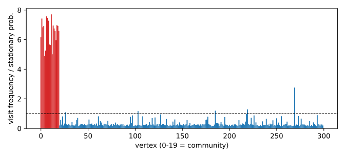
The sampled numbers are below. The exact averages \(\frac18\sum_{t=1}^{8}p_t/\pi\) give the same means, \(6.53\) and \(0.32\), and every vertex is within \(0.14\) of its sampled ratio.
\begin{equation*} \begin{aligned} \text{community: }&\ f_v/\pi_v\in[4.90,\,7.71],\ \text{mean } 6.53,\ \text{coefficient of variation } 0.13,\\ \text{rest: }&\ \text{mean } f_v/\pi_v=0.32,\\ &\ f( C)=0.707\ \text{versus}\ \pi( C)=0.108 . \end{aligned} \end{equation*}
The walk mixes inside the dense community within a couple of steps, but it leaks out only through the \(34\) boundary edges. So \(f\approx\lambda\,\pi|_C\) with \(\lambda\approx f( C)/\pi( C)\approx6.5\), which is the plateau. The residual ripple on the plateau comes from boundary vertices: a vertex with more edges to the outside has a larger \(\pi_v\) but no extra visits, so its ratio is lower (the correlation between ratio and inside-degree fraction is \(0.49\)). Outside \(C\) the ratio is below 1 except at a few vertices adjacent to \(C\), such as the spike of \(2.76\). Thresholding the ratio therefore recovers the community. As \(t\to\infty\) every ratio tends to 1 (Theorem 4.2), so the plateau only appears for short walks. \(\blacksquare\)
(1) Create a random graph with the following two structures imbedded in it. The first structure has three equal size communities with no edges between communities and the second structure has five equal size communities with no edges between communities. (2) Apply a clustering algorithm to find the dominant structure. Which structure did you get? (3) Weaken the dominant structure by removing a fraction of its edges and see if you can find the hidden structure.
Spectral clustering finds the 3-community structure exactly. Once about \(75\%\) of the edges inside the found communities are removed, it finds the hidden 5-community structure.
(1) Take \(n=300\). Structure 1 consists of the blocks \(\{0..99\},\{100..199\},\{200..299\}\), and each pair inside a block is joined with probability \(p_1=0.3\). Structure 2 is five blocks of \(60\) vertices, taken in a random permutation so that it is incoherent with structure 1, and each pair inside a block is joined with probability \(p_2=0.15\). The graph is the union of the two edge sets, so each structure on its own has no edges between its communities. (2) The clustering is the spectral clustering of Section 7.5: project the rows of \(A\) onto the top-\(k\) singular vectors, then run \(k\)-means. The top singular values are \(38.3,\,29.9,\,29.0\), followed by \(11.7,10.9,10.6,10.5,10.5\). These match the expected matrix, whose eigenvalues are approximately \(100p_1+60p_2=39\) (the shared all-ones direction), \(100p_1=30\) twice, and \(60p_2=9\) four times, plus noise. With \(k=3\) the adjusted Rand index (ARI) against structure 1 is \(1.000\) and against structure 2 is \(0.005\), so the algorithm returns the dominant structure. Even with \(k=5\) the result is dominated by structure 1 (ARI \(0.738\) against it, \(0.092\) against structure 2). (3) Remove each edge inside a found 3-community independently with probability \(f\), then rerun with \(k=5\):
| \(f\) | ARI vs hidden (5) | ARI vs dominant (3) |
|---|---|---|
| 0.25 | 0.059 | 0.737 |
| 0.50 | 0.082 | 0.743 |
| 0.75 | 0.893 | 0.010 |
| 0.90 | 0.942 | 0.004 |
Weakening scales the dominant block signal to about \(30(1-f)\). At \(f=0.5\) the second and third singular values are \(14.4,14.3\), with vectors lying mostly in the span of the structure-1 indicators, so they still crowd the top five. At \(f=0.75\) the dominant signal \(7.5\) has sunk into the noise. Singular values 2 to 5 are then \(9.2,8.7,8.5,8.1\), with vectors lying mostly in the structure-2 span, so \(k\)-means recovers structure 2 almost perfectly. This is the weaken-and-recluster procedure of Section 7.12.
import numpy as np
from sklearn.cluster import KMeans
from sklearn.metrics import adjusted_rand_score as ari
rng = np.random.default_rng(1)
n, p1, p2 = 300, 0.30, 0.15
g1 = np.repeat(np.arange(3), n // 3)
g2 = rng.permutation(np.repeat(np.arange(5), n // 5))
E1 = np.triu((g1[:, None] == g1) & (rng.random((n, n)) < p1), 1)
E2 = np.triu((g2[:, None] == g2) & (rng.random((n, n)) < p2), 1)
A = E1 | E2; A = (A | A.T).astype(float)
def spec(A, k):
    U, s, Vt = np.linalg.svd(A)
    return KMeans(k, n_init=20, random_state=0).fit_predict(U[:, :k] * s[:k])
def weaken(A, lab, keep):
    M = np.triu(rng.random(A.shape) < keep, 1); M = M | M.T
    return A * np.where(lab[:, None] == lab, M, 1)
d = spec(A, 3); print(ari(g1, d), ari(g2, d))
for f in (0.25, 0.5, 0.75, 0.9):
    l = spec(weaken(A, d, 1 - f), 5); print(f, ari(g2, l), ari(g1, l))
\(\blacksquare\)
Experiment with finding hidden communities.
Weaken-and-recluster (Section 7.12) recovers a hidden structure when its spectral signal is clearly weaker than the dominant one but not far below the noise edge \(2\sqrt{n\bar p}\). Alternating the procedure then sharpens both levels.
Setup. Take \(n=600\) vertices with background edge probability \(q=0.01\). The dominant structure is \(3\) blocks of \(200\) vertices, adding \(p_1=0.06\) to the edge probability of pairs inside a block. The hidden structure is \(4\) blocks of \(150\) vertices in a random permutation, adding \(p_2\). Each block contributes an eigenvalue of about \((\text{block size})\cdot(\text{added probability})\): \(12\) for the dominant blocks and \(150p_2\) for the hidden ones. The random part contributes a spectral norm of about \(2\sqrt{n\bar p}\approx 10\), where \(\bar p\) is the realised edge density.
Method. Run spectral clustering with \(k=3\) to get \(D_0\). Thin the edges inside the clusters of \(D_0\) down to the density outside them, and recluster with \(k=4\) to get \(H_1\). Go back to the original graph, thin the edges inside the clusters of \(H_1\), and recluster with \(k=3\) to get \(D_1\). Repeat this alternation. The table gives the ARI of each clustering against the true structure it targets.
import numpy as np
from scipy.sparse.linalg import eigsh
from sklearn.cluster import KMeans
from sklearn.metrics import adjusted_rand_score as ari
def spec(A, k):
    w, V = eigsh(A, k, which='LA'); return KMeans(k, n_init=20, random_state=0).fit_predict(V * w)
def weaken(A, lab, rng):          # thin edges inside found clusters to the outside density
    S = lab[:, None] == lab; keep = A[~S].mean() / A[S].mean()
    M = np.triu(rng.random(A.shape) < keep, 1); M = M | M.T
    return A * np.where(S, M, 1)
def run(p1, p2, q=0.01, n=600):
    rng = np.random.default_rng(7)
    gD = np.repeat(np.arange(3), n // 3); gH = rng.permutation(np.repeat(np.arange(4), n // 4))
    P = q + p1 * (gD[:, None] == gD) + p2 * (gH[:, None] == gH)
    A = np.triu(rng.random((n, n)) < P, 1); A = (A | A.T).astype(float)
    D = spec(A, 3); out = [ari(gD, D)]
    for r in range(2):            # alternate: weaken D -> find H; weaken H -> refind D
        H = spec(weaken(A, D, rng), 4); D = spec(weaken(A, H, rng), 3)
        out += [ari(gH, H), ari(gD, D)]
    print(p1, p2, np.round(out, 3))
for p2 in (0.04, 0.06, 0.08, 0.10): run(0.06, p2)
| \(p_2\) | hidden signal \(150p_2\) | noise \(2\sqrt{n\bar p}\) | \(D_0\) | \(H_1\) | \(D_1\) | \(H_2\) | \(D_2\) |
|---|---|---|---|---|---|---|---|
| 0.04 | 6.0 | 9.7 | 0.980 | 0.298 | 0.965 | 0.367 | 0.941 |
| 0.06 | 9.0 | 10.3 | 0.946 | 0.735 | 0.970 | 0.837 | 0.960 |
| 0.08 | 12.0 | 10.9 | 0.229 | 0.260 | 0.209 | 0.274 | 0.154 |
| 0.10 | 15.0 | 11.4 | 0.006 | 0.125 | 0.006 | 0.095 | 0.006 |
The ARI of the hidden structure found directly with \(k=4\) on the unweakened graph, at \(p_2=0.04\), is only \(0.024\).
Each row of the table shows a different regime.
- (i) \(p_2=0.04\): the hidden signal \(6\) is well below the noise edge \(9.7\). Weakening still lifts the hidden ARI from \(0.02\) to about \(0.3\), but recovery stays partial. Thinning also removes many of the hidden edges that lie inside dominant blocks (a third of all hidden edges), which weakens the hidden signal further.
- (ii) \(p_2=0.06\): the hidden signal \(9\) is just below the noise edge \(10.3\). Weakening finds the hidden structure (ARI \(0.735\)), and one more alternation improves it to \(0.837\). Removing the hidden structure also sharpens the dominant one, from \(0.946\) to \(0.970\). This is the “go back and weaken the hidden structure” improvement described in Section 7.12.
- (iii) \(p_2=0.08\): the two signals are equal (\(12\)). The top singular space mixes the 3- and 4-block indicators, so neither structure is “dominant” and both ARIs stay below \(0.3\).
- (iv) \(p_2=0.10\): the 4-block structure is now the dominant one. Clustering with \(k=3\) no longer matches structure 1 (ARI \(0.006\)), and weakening the wrong partition gains nothing. \(\blacksquare\)
Generate a bloc model with two equal size communities where \(p\) and \(q\) are the probabilities for the edge density within communities and the edge density between communities. Then generate a GNP model with probability \((p+q)/2\). Which of the two models most likely generates a community with half of the vertices?
The bloc model, overwhelmingly so once \(n\) is moderately large. Write \(r=\frac{p+q}{2}\). Let \(N_{\rm in}=2\binom{n/2}{2}\) be the number of pairs inside a half and \(N_{\rm out}=n^2/4\) the number of crossing pairs. For a bisection \(S\), let \(\Lambda(S)=\log\frac{P_{p,q}(G\mid S)}{P_r(G)}\) be the log-likelihood ratio (LLR) of the bloc model with communities \(S,\bar S\) against \(G(n,r)\), as described at the end of Section 7.5.5.
Bloc graph. If \(G\) comes from the bloc model with communities \(S\), then
\begin{equation*} \begin{aligned} \mathbb E\,\Lambda(S)&=N_{\rm in}\,\mathrm{KL}(p\Vert r)+N_{\rm out}\,\mathrm{KL}(q\Vert r)=:K\\ &\approx\tfrac{n^2}{4}\bigl(\mathrm{KL}(p\Vert r)+\mathrm{KL}(q\Vert r)\bigr). \end{aligned} \end{equation*}
\(G(n,r)\) graph. If \(G\sim G(n,r)\), then for each fixed \(S\) we have \(\mathbb E_r\,e^{\Lambda(S)}=1\), so Markov’s inequality gives \(P_r(\Lambda(S)\ge t)\le e^{-t}\). A union bound over the fewer than \(2^n\) bisections gives
\begin{equation*} P_r\Bigl(\max_S\Lambda(S)\ge t\Bigr)\le 2^n e^{-t}. \end{equation*}
So \(G(n,r)\) produces a half-size community as convincing as a bloc-model one with probability at most \(2^ne^{-K}=e^{-\Theta(n^2)}\). The comparison becomes decisive once \(K>n\ln2\), i.e. once \(n>4\ln 2/(\mathrm{KL}(p\Vert r)+\mathrm{KL}(q\Vert r))\).
Experiment. We took \(p=0.10\), \(q=0.05\), so \(r=0.075\) and \(\mathrm{KL}(p\Vert r)+\mathrm{KL}(q\Vert r)=0.00917\), which puts the threshold at \(n\approx302\). In the \(G(n,r)\) graph the half-size community is the best one found by spectral bisection (the second eigenvector split at its median), and \(\Lambda\) uses the true \((p,q)\):
import numpy as np
rng = np.random.default_rng(0)
n, p, q = 200, 0.10, 0.05; r = (p + q) / 2
g = np.repeat([0, 1], n // 2)
def graph(P): A = np.triu(rng.random((n, n)) < P, 1); return (A | A.T).astype(float)
def ll(e, N, x): return e * np.log(x) + (N - e) * np.log(1 - x)
def llr(A, lab, pq=None):          # log P(G | bloc) - log P(G | G(n,r))
    S = np.triu(lab[:, None] == lab, 1); X = np.triu(lab[:, None] != lab)
    ei, eo = A[S].sum(), A[X].sum(); Ni, No = S.sum(), X.sum()
    pi_, qi = pq if pq else (ei / Ni, eo / No)          # given (p,q) or fitted
    return ll(ei, Ni, pi_) + ll(eo, No, qi) - ll(ei + eo, Ni + No, r), ei / Ni, eo / No
def bisect(A):                     # spectral bisection: split 2nd eigenvector at its median
    w, V = np.linalg.eigh(A); v = V[:, -2]; return (v > np.median(v)).astype(int)
B, G = graph(np.where(g[:, None] == g, p, q)), graph(r)
print('bloc, planted  ', llr(B, g, (p, q)), llr(B, g))
print('bloc, spectral ', llr(B, bisect(B), (p, q)))
print('gnp, spectral  ', llr(G, bisect(G), (p, q)), llr(G, bisect(G)))
kl = lambda a, b: a * np.log(a / b) + (1 - a) * np.log((1 - a) / (1 - b))
Ni, No = 2 * (n // 2) * (n // 2 - 1) / 2, (n // 2) ** 2
print('theory', Ni * kl(p, r) + No * kl(q, r))
| \(n\) | \(K\) | \(n\ln 2\) | bloc, planted halves | bloc, spectral halves | \(G(n,r)\), spectral halves |
|---|---|---|---|---|---|
| 200 | 91.3 | 138.6 | 113.4 | 131.3 | 83.4 |
| 400 | 366.0 | 277.3 | 396.6 | 397.4 | 110.3 |
| 800 | 1465.7 | 554.5 | 1486.2 | 1481.7 | -154.5 |
The densities inside and across the halves in the bloc graphs were \((0.106,0.049)\), \((0.101,0.049)\) and \((0.101,0.050)\). In the \(G(n,r)\) graphs the best halves found had \((0.097,0.050)\), \((0.092,0.059)\) and \((0.087,0.064)\).
The planted LLR tracks \(K\propto n^2\). The \(G(n,r)\) value stays below the \(n\ln2\) ceiling and becomes negative at \(n=800\). In other words, spectral bisection of a random graph finds a half-size “community” whose contrast shrinks toward \(r\) as \(n\) grows, as expected when there is no planted signal. At \(n=200\) (below the threshold) the two cases are close (\(113\) against \(83\)), and a single graph cannot be classified reliably there. Above the threshold, a half-size community with densities \(p,q\) is \(e^{\Theta(n^2)}\) times more likely to come from the bloc model. \(\blacksquare\)
Random Graphs
Exercises 8.1–8.7
Search the World Wide Web to find some real world graphs in machine readable form or data bases that could automatically be converted to graphs. (1) Plot the degree distribution of each graph. (2) Count the number of connected components of each size in each graph. (3) Count the number of cycles in each graph. (4) Describe what you find. (5) What is the average vertex degree in each graph? If the graph were a \(G(n,p)\) graph, what would the value of \(p\) be? (6) Spot differences between your graphs and \(G(n,p)\) for \(p\) from Item 5. Look at sizes of connected components, cycles, size of giant component.
All three real graphs are connected, have far more triangles and a far larger maximum degree than \(G(n,p)\) at the matched \(p\), and have heavy-tailed rather than binomial degree distributions. The run was offline, so the graphs are three machine-readable real networks available locally: Zachary’s karate club and the Les Miserables character co-occurrence network (both bundled with networkx), and the undirected package-dependency graph of a local Anaconda install (512 packages plus 11 virtual dependency names, an edge whenever one package declares the other as a dependency). Listing all simple cycles takes exponential time, so for Item 3 we report the cycle rank \(m-n+c\) (the number of independent cycles, i.e. edges beyond a spanning forest) and the number of triangles. Each graph was compared with 200 samples of \(G(n,p)\) with \(p = \bar d/(n-1)\), using seeded generators.
(1) Degree distributions (log-log):
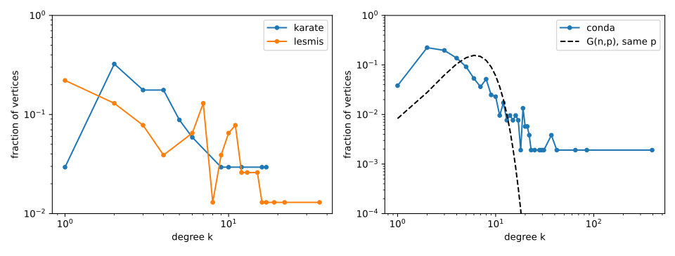
2.–5. The measured values:
| graph | \(n\) | \(m\) | components | avg degree \(\bar d\) | \(p=\bar d/(n-1)\) | max degree | cycle rank | triangles |
|---|---|---|---|---|---|---|---|---|
| karate | 34 | 78 | one of 34 | 4.59 | 0.1390 | 17 | 45 | 45 |
| Les Mis | 77 | 254 | one of 77 | 6.60 | 0.0868 | 36 | 178 | 467 |
| conda deps | 523 | 1741 | one of 523 | 6.66 | 0.0128 | 394 | 1219 | 1674 |
(4) In every graph a few hubs carry a large share of the edges: the instructor and president in the karate club (degrees 16 and 17), Valjean in Les Miserables (36), and python in the dependency graph (394 of 522 possible neighbours, ahead of libcxx at 85), while the median degrees are only \(3\), \(6\) and \(4\). The dependency graph’s distribution falls off roughly like a power law across two decades. All three are highly clustered: two neighbours of a vertex tend to be adjacent (friends of friends, characters sharing scenes, packages in one software stack).
(6) The averages over 200 samples of \(G(n,p)\) with the same \(n\) and \(p\):
| graph | giant component | components | cycle rank | triangles | max degree | transitivity (real / \(G(n,p)\)) |
|---|---|---|---|---|---|---|
| karate | 33.7 | 1.26 | 45.3 | 16.0 | 9.0 | 0.256 / 0.135 |
| Les Mis | 76.9 | 1.10 | 177.9 | 48.1 | 13.3 | 0.499 / 0.087 |
| conda deps | 522.4 | 1.63 | 1213.9 | 48.8 | 15.8 | 0.051 / 0.013 |
- Components and giant component. \(\bar d > 1\) in every case, so \(G(n,p)\) also has a giant component covering almost every vertex (Section 8.3). The only difference is the occasional isolated vertex in \(G(n,p)\); the real graphs have none, because every package or character is by construction tied to something.
- Cycles. The cycle rank is \(m-n+c\) and \(m\) is matched, so it agrees by construction. The short cycles differ: the expected triangle count of \(G(n,p)\) is \(\binom n3 p^3 \approx \bar d^3/6\) (Section 8.1.2), giving \(16\), \(48\) and \(49\). The real graphs have \(45\), \(467\) and \(1674\) triangles, about \(3\) to \(34\) times as many.
- Degrees. Theorem 8.1 concentrates \(G(n,p)\) degrees within \(O(\sqrt{np})\) of \(np\), and the maximum degree is only \(9\)–\(16\). The real maxima are \(17\), \(36\) and \(394\). In the right panel the binomial pmf of \(G(n,p)\) has fallen below \(10^{-4}\) by \(k=19\), while the conda graph still has vertices of degree \(19\)–\(394\). That is the heavy tail of Section 8.1.1, which \(G(n,p)\) cannot produce.
In \(G(n,p)\) the probability of a vertex having degree \(k\) is \(\binom nk p^k(1-p)^{n-k}\). (1) Show by direct calculation that the expected degree is \(np\). (2) Compute directly the variance of the degree distribution. (3) Where is the mode of the binomial distribution for a given value of \(p\)? The mode is the point at which the probability is maximum.
The mean is \(np\), the variance is \(np(1-p)\), and for \(0<p<1\) the mode is \(\lfloor (n+1)p\rfloor\). When \((n+1)p\) is an integer, \((n+1)p-1\) is a mode as well. Write \(P(k)=\binom nk p^k(1-p)^{n-k}\), \(q=1-p\), and use \(k\binom nk = n\binom{n-1}{k-1}\) together with the binomial theorem.
(1) Mean:
\begin{equation*} \begin{aligned} \sum_{k=0}^n kP(k) &= np\sum_{k=1}^{n}\binom{n-1}{k-1}p^{k-1}q^{(n-1)-(k-1)}\\ &= np\,(p+q)^{n-1} = np . \end{aligned} \end{equation*}
(2) Variance. Applying the same identity twice, \(k(k-1)\binom nk = n(n-1)\binom{n-2}{k-2}\), so
\begin{equation*} \begin{aligned} \sum_{k} k(k-1)P(k) &= n(n-1)p^2(p+q)^{n-2} = n(n-1)p^2,\\ \operatorname{Var} &= \sum_k k(k-1)P(k) + np - (np)^2\\ &= n(n-1)p^2 + np - n^2p^2 = np(1-p). \end{aligned} \end{equation*}
(3) Mode. For \(0\le k<n\),
\begin{equation*} \frac{P(k+1)}{P(k)} = \frac{(n-k)\,p}{(k+1)\,q} \ge 1 \iff (n-k)p \ge (k+1)(1-p) \iff k+1 \le (n+1)p . \end{equation*}
So \(P\) strictly increases up to \(k=\lfloor (n+1)p\rfloor\) and strictly decreases after it. The mode is therefore \(\lfloor (n+1)p\rfloor\), within \(1\) of the mean \(np\). When \((n+1)p\) is an integer the ratio at \(k=(n+1)p-1\) equals \(1\), and the two values \((n+1)p-1\) and \((n+1)p\) tie. \(\blacksquare\)
(1) Plot the degree distribution for \(G(1000, 0.003)\). (2) Plot the degree distribution for \(G(1000, 0.030)\).
In both graphs the empirical degree histogram follows the binomial \(\mathrm{Bin}(999,p)\) curve of Section 8.1.1. For \(p=0.003\) it is a skewed, Poisson-like distribution with mean about \(3\). For \(p=0.030\) it is a nearly symmetric bell around \(30\). One graph was sampled for each \(p\) (seed 1), and its degree histogram is plotted against the pmf:
import numpy as np, networkx as nx, matplotlib.pyplot as plt
from scipy.stats import binom
fig, ax = plt.subplots(1, 2, figsize=(10, 3.8))
for a, p in zip(ax, [0.003, 0.030]):
    G = nx.gnp_random_graph(1000, p, seed=1)
    deg = np.array([d for _, d in G.degree()])
    k = np.arange(deg.max() + 2)
    a.bar(k, np.bincount(deg, minlength=len(k)) / 1000, alpha=.6, label='G(1000, %.3f)' % p)
    a.plot(k, binom.pmf(k, 999, p), 'ko-', ms=3, label='Binomial(999, p)')
    a.set_xlabel('degree k'); a.set_ylabel('fraction of vertices'); a.legend()
plt.savefig('fds-ch08-gnpdeg.svg')
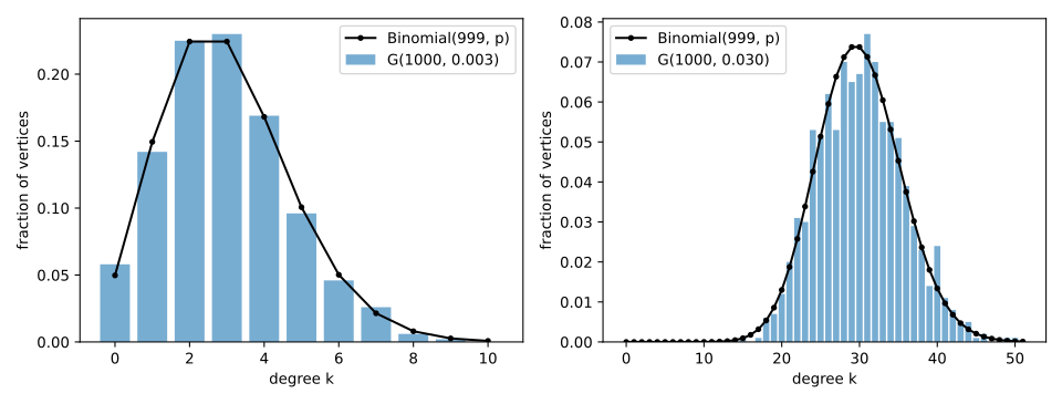
(1) \(G(1000,0.003)\): the expected degree is \(999p = 2.997\) and the variance is \(999p(1-p)=2.988\) (Exercise 8.2). The sample has mean \(2.962\), variance \(2.919\), degrees from \(0\) to \(9\) and mode \(3\). Of the vertices, \(58\) are isolated; the prediction is \(1000(1-p)^{999}\approx 49.7\). This is the sparse regime \(p=d/n\) with \(d=3\), where the binomial is close to the Poisson law \(e^{-3}3^k/k!\).
(2) \(G(1000,0.030)\): the expected degree is \(29.97\) and the variance is \(29.07\). The sample has mean \(30.16\), variance \(29.99\), mode \(31\), and degrees from \(15\) to \(50\), with no isolated vertices. Every degree lies within \(3.7\sqrt{np}\) of \(np\), and the distribution is close to the normal \(N(30,\,29)\).
To better understand the binomial distribution plot \(\binom nk p^k(1-p)^{n-k}\) as a function of \(k\) for \(n=50\) and \(k = 0.05, 0.5, 0.95\). For each value of \(p\) check the sum over all \(k\) to ensure that the sum is one.
In floating point the three sums are \(0.999999999999998\), \(1.0\) and \(1.0\), which is one up to rounding error. The printed “\(k = 0.05, 0.5, 0.95\)” should read \(p = 0.05, 0.5, 0.95\), and we use that.
import numpy as np, matplotlib.pyplot as plt
from math import comb
n = 50; k = np.arange(n + 1)
for p in [0.05, 0.5, 0.95]:
    P = np.array([comb(n, j) * p**j * (1 - p)**(n - j) for j in k])
    plt.plot(k, P, 'o-', ms=3, label='p = %.2f' % p)
    print(p, P.sum(), P.argmax())
plt.xlabel('k'); plt.legend(); plt.savefig('fds-ch08-binom50.svg')
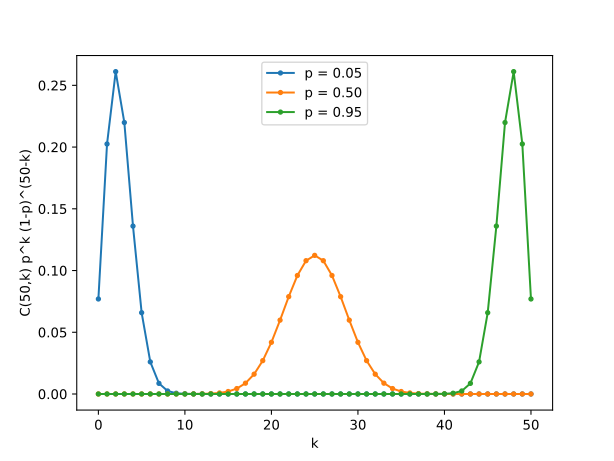
Exactly, the sum is one for every \(p\) by the binomial theorem:
\begin{equation*} \sum_{k=0}^{50}\binom{50}{k}p^k(1-p)^{50-k} = \bigl(p+(1-p)\bigr)^{50} = 1 . \end{equation*}
The three curves have their peaks at \(k=2\), \(25\) and \(48\), which are \(\lfloor 51p\rfloor\) as in Exercise 8.2. The peak heights are \(0.261\), \(0.112\) and \(0.261\); the outer curves are mirror images since \(P_p(k)=P_{1-p}(50-k)\).
In \(G\left(n,\frac1n\right)\), argue that with high probability there is no vertex of degree greater than \(\frac{6\log n}{\log\log n}\) (i.e., the probability that such a vertex exists goes to zero as \(n\) goes to infinity). You may use the Poisson approximation and may wish to use the fact that \(k! \ge \left(\frac ke\right)^k\).
The probability is at most \(1/n\) for every \(n\ge 3\), by a union bound over vertices and over possible sets of neighbours. With an exact tail bound we do not need the Poisson approximation. Take logarithms natural (any other base only changes \(\log n/\log\log n\) by a factor \(1+o(1)\), and the constant \(6\) leaves room for that), put \(t=6\ln n/\ln\ln n\), and let \(k=\lfloor t\rfloor+1\), so that “degree \(>t\)” means “degree \(\ge k\)”. A vertex \(v\) has degree \(\ge k\) only if, for some \(k\)-set \(S\) of other vertices, all \(k\) edges from \(v\) to \(S\) are present. So
\begin{equation*} \begin{aligned} \Pr(\deg v\ge k) &\le \binom{n-1}{k}\frac1{n^k} \le \frac{(n-1)^k}{k!\,n^k}\\ &\le \frac1{k!} \le \Bigl(\frac ek\Bigr)^k . \end{aligned} \end{equation*}
The function \(x\mapsto x\ln(x/e)\) is increasing for \(x>1\), and \(k\ge t\ge 6e>1\) because \(y/\ln y\ge e\) for \(y>1\). Using \(\ln 6>1\) and \(\ln y/y\le 1/e<\frac23\) with \(y=\ln\ln n\),
\begin{equation*} \begin{aligned} k\ln\frac ke \ge t\ln\frac te &= \frac{6\ln n}{\ln\ln n}\bigl(\ln 6-1+\ln\ln n-\ln\ln\ln n\bigr)\\ &\ge 6\ln n\Bigl(1-\frac{\ln\ln\ln n}{\ln\ln n}\Bigr) \ge 2\ln n . \end{aligned} \end{equation*}
The union bound over the \(n\) vertices then gives
\begin{equation*} \begin{aligned} \Pr\Bigl(\exists v:\ \deg v > \tfrac{6\ln n}{\ln\ln n}\Bigr) &\le n\Bigl(\frac ek\Bigr)^k\\ &\le n\cdot n^{-2} = \frac1n \to 0 . \qquad\blacksquare \end{aligned} \end{equation*}
The example of Section 8.1.1 showed that if the degrees in \(G\left(n,\frac1n\right)\) were independent there would almost surely be a vertex of degree \(\Omega(\log n/\log\log n)\). However, the degrees are not independent. Show how to overcome this difficulty.
Split the vertices into two halves \(A\) and \(B\) and count, for each \(a\in A\), only its edges into \(B\). Let \(|B|=m=\lfloor n/2\rfloor\) and \(|A|=n-m\ge n/2\), and for \(a\in A\) let \(d_B(a)\) be the number of edges from \(a\) to \(B\). Each \(d_B(a)\) is \(\mathrm{Bin}(m,1/n)\) and depends only on the \(m\) edges \(\{a,b\}\), \(b\in B\); these edge sets are disjoint for distinct \(a\), so the \(d_B(a)\), \(a\in A\), are independent.
Let \(k=\lceil \ln n/(2\ln\ln n)\rceil\) and \(q=\Pr(d_B(a)=k)\). For large \(n\) we have \(m-k\ge n/3\) and \(3k\le \ln n\). Then \(\binom mk\ge (m-k)^k/k!\), \((1-\frac1n)^{m-k}\ge(1-\frac1n)^n\ge\frac14\) and \(k!\le k^k\) give
\begin{equation*} \begin{aligned} q &= \binom mk\frac1{n^k}\Bigl(1-\frac1n\Bigr)^{m-k} \ge \frac{1}{4\cdot 3^k k!} \ge \frac{1}{4(3k)^k},\\ \ln\,(3k)^k &= k\ln(3k) \le \Bigl(\frac{\ln n}{2\ln\ln n}+1\Bigr)\ln\ln n\\ &= \tfrac12\ln n+\ln\ln n , \end{aligned} \end{equation*}
so \(q\ge 1/(4\sqrt n\,\ln n)\). Every vertex satisfies \(\deg a\ge d_B(a)\). By independence and \(1-q\le e^{-q}\),
\begin{equation*} \begin{aligned} \Pr\bigl(\text{every vertex has degree}<k\bigr) &\le \Pr\bigl(d_B(a)\ne k\ \ \forall a\in A\bigr) = (1-q)^{|A|}\\ &\le e^{-qn/2} \le \exp\Bigl(-\frac{\sqrt n}{8\ln n}\Bigr) \to 0 . \end{aligned} \end{equation*}
Hence almost surely some vertex has degree at least \(k\ge \frac12\ln n/\ln\ln n=\Omega(\log n/\log\log n)\). \(\blacksquare\)
Let \(f(n)\) be a function that is asymptotically less than \(n\). Some such functions are \(1/n\), a constant \(d\), \(\log n\) or \(n^{1/3}\). Show that
\begin{equation*} \Bigl(1+\frac{f(n)}{n}\Bigr)^n \simeq e^{f(n)(1\pm o(1))} \end{equation*}
for large \(n\). That is
\begin{equation*} \lim_{n\to\infty}\frac{\ln\Bigl[\bigl(1+\frac{f(n)}{n}\bigr)^n\Bigr]}{f(n)} = 1 . \end{equation*}
Put \(x_n=f(n)/n\). Then the ratio in question is \(\ln(1+x_n)/x_n\), which tends to \(1\) because \(x_n\to 0\). Here “asymptotically less than \(n\)” means \(f(n)/n\to 0\), and \(f(n)\ne 0\) so that the ratio is defined. Thus
\begin{equation*} \frac{\ln\bigl[(1+f(n)/n)^n\bigr]}{f(n)} = \frac{n\ln(1+x_n)}{n\,x_n} = \frac{\ln(1+x_n)}{x_n} . \end{equation*}
For \(|x|\le\frac12\) the Taylor series of \(\ln(1+x)\) gives
\begin{equation*} \begin{aligned} \bigl|\ln(1+x)-x\bigr| &= \Bigl|\sum_{j\ge 2}\frac{(-1)^{j+1}x^j}{j}\Bigr| \le \frac12\sum_{j\ge2}|x|^j\\ &= \frac{x^2}{2(1-|x|)} \le x^2 . \end{aligned} \end{equation*}
Since \(|x_n|\le\frac12\) for all large \(n\),
\begin{equation*} \Bigl|\frac{\ln(1+x_n)}{x_n}-1\Bigr| \le |x_n| = \frac{|f(n)|}{n} \to 0 . \end{equation*}
So \(\ln\bigl[(1+f(n)/n)^n\bigr] = f(n)(1+\varepsilon_n)\) with \(|\varepsilon_n|\le |f(n)|/n=o(1)\). Exponentiating,
\begin{equation*} \Bigl(1+\frac{f(n)}{n}\Bigr)^n = e^{f(n)(1\pm o(1))} . \qquad\blacksquare \end{equation*}
Exercises 8.8–8.14
(1) In the limit as \(n\) goes to infinity, how does \(\left(1-\frac1n\right)^{n\ln n}\) behave? (2) What is \(\displaystyle\lim_{n\to\infty}\left(\frac{n+1}{n}\right)^n\)?
(1) It tends to \(0\) like \(1/n\): \(\left(1-\frac1n\right)^{n\ln n} = \frac1n\,(1+o(1))\). Using \(\ln(1-x) = -x - \frac{x^2}{2} - O(x^3)\),
\begin{equation*} \begin{aligned} \ln\left(1-\tfrac1n\right)^{n\ln n} &= n\ln n\left(-\tfrac1n - \tfrac{1}{2n^2} - O(n^{-3})\right)\\ &= -\ln n - \frac{\ln n}{2n} - O\!\left(\frac{\ln n}{n^2}\right) = -\ln n + o(1), \end{aligned} \end{equation*}
so \(n\left(1-\frac1n\right)^{n\ln n} = e^{o(1)} \to 1\).
(2) \(\displaystyle\lim_{n\to\infty}\left(\frac{n+1}{n}\right)^n = \lim_{n\to\infty}\left(1+\frac1n\right)^n = e\), since
\begin{equation*} n\ln\left(1+\tfrac1n\right) = n\left(\tfrac1n - \tfrac{1}{2n^2} + O(n^{-3})\right) = 1 - \tfrac{1}{2n} + O(n^{-2}) \to 1 . \end{equation*}
Consider a random permutation of the integers \(1\) to \(n\). The integer \(i\) is said to be a fixed point of the permutation if \(i\) is the integer in the \(i^{\text{th}}\) position of the permutation. Use indicator variables to determine the expected number of fixed points in a random permutation.
The expected number of fixed points is \(1\), for every \(n\). Let \(\pi\) be uniform over the \(n!\) permutations, let \(I_i\) indicate \(\pi(i)=i\), and let \(x=\sum_{i=1}^n I_i\) count the fixed points. Exactly \((n-1)!\) permutations fix \(i\), so by linearity of expectation (which needs no independence of the \(I_i\)),
\begin{equation*} E(x) = \sum_{i=1}^n E(I_i) = \sum_{i=1}^n \frac{(n-1)!}{n!} = n\cdot\frac1n = 1 . \end{equation*}
Generate a graph \(G\left(n,\frac dn\right)\) with \(n=1000\) and \(d=2\), \(3\), and \(6\). Count the number of triangles in each graph. Try the experiment with \(n=100\).
One graph per setting (seed 2018) gave \(1\), \(2\), \(38\) triangles for \(n=1000\) and \(2\), \(1\), \(24\) triangles for \(n=100\) (\(d=2,3,6\)); averaging \(1000\) graphs per setting shows the count stays near \(\binom n3(d/n)^3\to d^3/6\) (Section 8.1.2) at both sizes:
import numpy as np, networkx as nx
from math import comb
rng = np.random.default_rng(2018)
for n in (1000, 100):
    for d in (2, 3, 6):
        tri = lambda: sum(nx.triangles(nx.fast_gnp_random_graph(
            n, d/n, seed=int(rng.integers(1e9)))).values()) // 3
        one = tri()
        many = [tri() for _ in range(1000)]
        print(n, d, one, round(comb(n, 3)*(d/n)**3, 3), np.mean(many))
| \(n\) | \(d\) | one graph | exact \(E(x)\) | \(d^3/6\) | mean of 1000 |
|---|---|---|---|---|---|
| 1000 | 2 | 1 | 1.329 | 1.333 | 1.250 |
| 1000 | 3 | 2 | 4.487 | 4.5 | 4.544 |
| 1000 | 6 | 38 | 35.892 | 36 | 35.947 |
| 100 | 2 | 2 | 1.294 | 1.333 | 1.334 |
| 100 | 3 | 1 | 4.366 | 4.5 | 4.399 |
| 100 | 6 | 24 | 34.927 | 36 | 35.366 |
What is the expected number of squares (4-cycles) in \(G\left(n,\frac dn\right)\)? What is the expected number of 4-cliques in \(G\left(n,\frac dn\right)\)? A 4-clique consists of four vertices with all \(\binom42\) edges present.
The expected number of 4-cycles is \(3\binom n4\left(\frac dn\right)^4 \to \frac{d^4}{8}\). The expected number of 4-cliques is \(\binom n4\left(\frac dn\right)^6 \sim \frac{d^6}{24n^2} \to 0\).
A set of \(4\) vertices carries \(3\) distinct 4-cycles, since there are \(4!/8\) cyclic orders up to rotation and reflection. Each 4-cycle needs \(4\) particular edges, which are present with probability \(p^4\). It carries exactly one 4-clique, which needs \(6\) edges. By linearity of expectation over these indicator variables, as in Section 8.1.2,
\begin{equation*} \begin{aligned} E(\#\text{4-cycles}) &= 3\binom n4\frac{d^4}{n^4} = \frac{(n-1)(n-2)(n-3)}{8n^3}\,d^4 \to \frac{d^4}{8},\\ E(\#\text{4-cliques}) &= \binom n4\frac{d^6}{n^6} = \frac{(n-1)(n-2)(n-3)}{24n^5}\,d^6 \sim \frac{d^6}{24n^2}. \end{aligned} \end{equation*}
Carry out an argument, similar to the one used for triangles, to show that \(p=\frac{1}{n^{2/3}}\) is a threshold for the existence of a 4-clique. A 4-clique consists of four vertices with all \(\binom42\) edges present.
Let \(x=\sum_S \Delta_S\), where \(S\) ranges over the \(4\)-subsets of vertices and \(\Delta_S\) indicates that all \(6\) edges inside \(S\) are present. Then \(E(x)=\binom n4 p^6\).
(i) Suppose \(p = o(n^{-2/3})\). Then \(E(x)\le n^4p^6/24 = (pn^{2/3})^6/24 \to 0\), and by Markov’s inequality (the first moment method of Section 8.2) \(\operatorname{Prob}(x\ge1)\le E(x)\to0\). So almost surely there is no 4-clique.
(ii) Suppose \(pn^{2/3}\to\infty\). Then \(E(x)\ge n^4p^6/30\to\infty\) (for large \(n\), \(\binom n4\ge n^4/30\)). We split \(E(x^2)=\sum_{S,T}E(\Delta_S\Delta_T)\) by \(k=|S\cap T|\):
- \(k\le1\): the two 4-sets share no edge, so \(\Delta_S\) and \(\Delta_T\) are independent and these terms sum to at most \(E^2(x)\).
- \(k=2\): there are at most \(\binom n4\binom42\binom{n-4}2\le n^6/8\) such pairs, and they span \(11\) edges, giving a total of at most \(n^6p^{11}/8\).
- \(k=3\): there are at most \(\binom n4\cdot4\cdot(n-4)\le n^5/6\) pairs, spanning \(9\) edges, giving at most \(n^5p^9/6\).
- \(k=4\): here \(S=T\), and these terms sum to \(E(x)\).
With \(E^2(x)\ge n^8p^{12}/900\) this gives
\begin{equation*} \begin{aligned} \frac{\operatorname{Var}(x)}{E^2(x)} = \frac{E(x^2)-E^2(x)}{E^2(x)} &\le \frac{900\,n^6p^{11}/8}{n^8p^{12}} + \frac{900\,n^5p^{9}/6}{n^8p^{12}} + \frac{1}{E(x)}\\ &= \frac{112.5}{n^2p} + \frac{150}{(np)^3} + \frac{1}{E(x)} \to 0 . \end{aligned} \end{equation*}
Each term vanishes: \(n^2p\ge n^{4/3}\to\infty\), \(np \ge n^{1/3}\to\infty\) (both for large \(n\)), and \(E(x)\to\infty\). Since \(E(x)>0\) and \(\operatorname{Var}(x)=o(E^2(x))\), Theorem 8.3 gives that \(x>0\) almost surely.
Together, (i) and (ii) show that \(p=n^{-2/3}\) is a threshold for the existence of a 4-clique.
What is the expected number of simple paths of length \(3\), \(\log n\), \(\sqrt n\), and \(n-1\) in \(G\left(n,\frac dn\right)\)? A simple path is a path where no vertex appears twice as in a cycle. The expected number of simple paths of a given length being infinite does not imply that a graph selected at random has such a path.
A path of length \(k\) has \(k\) edges on \(k+1\) distinct vertices. \(K_n\) contains \(n(n-1)\cdots(n-k)/2\) such paths: ordered vertex sequences, with each path counted once per direction. Each path is present with probability \((d/n)^k\), so by linearity
\begin{equation*} E(x_k) = \frac{n(n-1)\cdots(n-k)}{2}\left(\frac dn\right)^k = \frac{n\,d^k}{2}\prod_{i=1}^{k}\left(1-\frac in\right). \end{equation*}
Let \(P_k=\prod_{i=1}^k(1-i/n)\). Then \(\ln P_k = -\frac{k(k+1)}{2n} - O\!\left(\frac{k^3}{n^2}\right)\) for \(k\le n/2\). Take \(\log=\ln\); for \(\log_2\), replace \(n^{\ln d}\) by \(n^{\log_2 d}\).
- \(k=3\): \(E(x_3) = \frac{(n-1)(n-2)(n-3)}{2n^2}\,d^3 \sim \frac{d^3 n}{2}\).
- \(k=\ln n\): \(\ln P_k = O(\ln^2 n/n)\to0\), so \(E(x_k)\sim \frac n2 d^{\ln n} = \frac12 n^{1+\ln d}\).
- \(k=\sqrt n\): \(\ln P_k = -\frac12 + O(n^{-1/2})\), so \(E(x_k)\sim \frac{n\,d^{\sqrt n}}{2\sqrt e}\).
- \(k=n-1\) (Hamilton paths): \(E(x_{n-1}) = \frac{n!}{2}\left(\frac dn\right)^{n-1}\), and Stirling’s formula \(n!\sim\sqrt{2\pi n}\,(n/e)^n\) gives
\begin{equation*} E(x_{n-1}) \sim \frac{\sqrt{2\pi}\,n^{3/2}}{2d}\left(\frac de\right)^n . \end{equation*}
So the expected number tends to infinity in these cases: \(k=3\) for every \(d>0\); \(k=\ln n\) for \(d>1/e\); \(k=\sqrt n\) for \(d\ge1\); and \(k=n-1\) for \(d\ge e\). The last case is the warning in the statement: for constant \(d\), \(p=d/n=o(\ln n/n)\) lies below the sharp threshold of Theorem 8.6, so \(G(n,d/n)\) almost surely has an isolated vertex and hence no Hamilton path, although for \(d\ge e\) the expected number of Hamilton paths is infinite in the limit.
Let \(x\) be an integer chosen uniformly at random from \(\{1,2,\ldots,n\}\). Count the number of distinct prime factors of \(n\). The exercise is to show that the number of prime factors almost surely is \(\Theta(\ln\ln n)\). Let \(p\) stand for a prime number between \(2\) and \(n\). (1) For each fixed prime \(p\), let \(I_p\) be the indicator function of the event that \(p\) divides \(x\). Show that \(E(I_p)=\frac1p+O\left(\frac1n\right)\). (2) The random variable of interest, \(y=\sum_p I_p\), is the number of prime divisors of \(x\) picked at random. Show that the variance of \(y\) is \(O(\ln\ln n)\). For this, assume the known result that the number of primes \(p\) between \(2\) and \(n\) is \(O(n/\ln n)\) and that \(\sum_p\frac1p=\ln\ln n\). To bound the variance of \(y\), think of what \(E(I_pI_q)\) is for \(p\ne q\), both primes. (3) Use (1) and (2) to prove that the number of prime factors is almost surely \(\Theta(\ln\ln n)\).
Erratum: the count intended is of the prime factors of \(x\), not of \(n\). Write \(\pi(n)=O(n/\ln n)\) for the number of primes up to \(n\).
(1) The multiples of \(p\) in \(\{1,\ldots,n\}\) number \(\lfloor n/p\rfloor\), so
\begin{equation*} E(I_p) = \frac{\lfloor n/p\rfloor}{n}\in\left(\frac1p-\frac1n,\ \frac1p\right] \quad\Longrightarrow\quad E(I_p)=\frac1p+O\!\left(\frac1n\right). \end{equation*}
(2) For distinct primes \(p\ne q\), \(I_pI_q\) indicates \(pq\mid x\), so \(E(I_pI_q)=\lfloor n/pq\rfloor/n\le \frac1{pq}\). Together with part 1,
\begin{equation*} \operatorname{Cov}(I_p,I_q) \le \frac1{pq} - \left(\frac1p-\frac1n\right)\left(\frac1q-\frac1n\right) \le \frac1n\left(\frac1p+\frac1q\right). \end{equation*}
Also \(\operatorname{Var}(I_p)\le E(I_p^2)=E(I_p)\le \frac1p\). Summing over ordered pairs,
\begin{equation*} \begin{aligned} \operatorname{Var}(y) &= \sum_p \operatorname{Var}(I_p) + \sum_{p\ne q}\operatorname{Cov}(I_p,I_q) \le \sum_p\frac1p + \frac{2\pi(n)}{n}\sum_p\frac1p\\ &= \ln\ln n + O\!\left(\frac{\ln\ln n}{\ln n}\right) = O(\ln\ln n). \end{aligned} \end{equation*}
(3) By part 1, \(E(y)=\sum_p\frac1p + O(\pi(n)/n) = \ln\ln n + O(1/\ln n)\). Chebyshev’s inequality and part 2 then give
\begin{equation*} \operatorname{Prob}\left(|y-E(y)|\ge\tfrac12\ln\ln n\right) \le \frac{4\operatorname{Var}(y)}{(\ln\ln n)^2} = O\!\left(\frac{1}{\ln\ln n}\right)\to 0 . \end{equation*}
So almost surely \(\left(\frac12-o(1)\right)\ln\ln n\le y\le\left(\frac32+o(1)\right)\ln\ln n\). That is, the number of distinct prime factors of \(x\) is almost surely \(\Theta(\ln\ln n)\).
Exercises 8.15–8.21
Suppose one hides a clique of size \(k\) in a random graph \(G\left(n,\frac12\right)\). I.e., in the random graph, choose some subset \(S\) of \(k\) vertices and put in the missing edges to make \(S\) a clique. Presented with the modified graph, the goal is to find \(S\). The larger \(S\) is, the easier it should be to find. In fact, if \(k\) is more than \(c\sqrt{n\ln n}\), then with high probability the clique leaves a telltale sign identifying \(S\) as the \(k\) vertices of largest degree. Prove this statement by appealing to Theorem 8.1. It remains a puzzling open problem to find such hidden cliques when \(k\) is smaller, say, \(O(n^{1/3})\).
With \(c=12\) (any \(c>8\sqrt2\) works) and \(S\) fixed before the graph is drawn, every vertex of \(S\) ends up with larger degree than every vertex outside \(S\), with probability at least \(1-6/n\).
Write \(d_0(v)\) for the degree of \(v\) in the original \(G(n,\frac12)\), and \(d_{\rm in}(v)\) for the number of original edges from \(v\in S\) into \(S\). After planting, \(v\notin S\) keeps degree \(d_0(v)\), and \(v\in S\) has degree \(d_0(v)+(k-1-d_{\rm in}(v))\). Apply Theorem 8.1 with \(p=\frac12\) and \(\alpha=4\sqrt{\ln n}\) (this is in \((0,\sqrt{n/2})\) for large \(n\)) to each vertex of \(G(n,\frac12)\). Apply it again with \(n\) replaced by \(k\) to each vertex of the induced graph on \(S\), which is a \(G(k,\frac12)\) (here \(\alpha<\sqrt{k/2}\) because \(k\ge12\sqrt{n\ln n}>32\ln n\)). The union bound over the \(n+k\) vertices gives
\begin{equation*} \begin{aligned} &\Big|d_0(v)-\tfrac n2\Big|<\Delta:=\sqrt{8n\ln n}\ \ \forall v, \qquad d_{\rm in}(v)<\tfrac k2+\sqrt{8k\ln n}\ \ \forall v\in S,\\ &\text{failure probability}\le 3(n+k)e^{-2\ln n}\le 6/n . \end{aligned} \end{equation*}
On this event, for \(u\in S\) and \(w\notin S\),
\begin{equation*} \begin{aligned} \deg(u)-\deg(w)&>\Big(\tfrac n2-\Delta+\tfrac k2-1-\sqrt{8k\ln n}\Big)\\ &\quad-\Big(\tfrac n2+\Delta\Big)\\ &=\tfrac k2-2\sqrt{8n\ln n}-1-\sqrt{8k\ln n}. \end{aligned} \end{equation*}
Here \(\sqrt{8k\ln n}+1=o(k)\), and \(k\ge 12\sqrt{n\ln n}\) gives \(\frac k2\ge 6\sqrt{n\ln n}>2\sqrt8\sqrt{n\ln n}\approx5.66\sqrt{n\ln n}\). So the difference is positive for large \(n\). Hence with high probability the \(k\) vertices of largest degree are exactly \(S\). \(\blacksquare\)
The clique problem in a graph is to find the maximal size clique. This problem is known to be NP-hard and so a polynomial time algorithm is thought unlikely. We can ask the corresponding question about random graphs. For example, in \(G\left(n,\frac12\right)\) there almost surely is a clique of size \((2-\varepsilon)\log n\) for any \(\varepsilon>0\). But it is not known how to find one in polynomial time. (1) Show that in \(G(n,\frac12)\) there almost surely are no cliques of size greater than or equal to \(2\log_2 n\). (2) Use the second moment method to show that in \(G(n,\frac12)\), almost surely there are cliques of size \((2-\varepsilon)\log_2 n\). (3) Show that for any \(\varepsilon>0\), a clique of size \((2-\varepsilon)\log n\) can be found in \(G\left(n,\frac12\right)\) in time \(n^{O(\ln n)}\) if one exists. (4) Give an \(O(n^2)\) algorithm that finds a clique of size \(\Omega(\log n)\) in \(G(n,\frac12)\) with high probability. Hint: use a greedy algorithm. Apply your algorithm to \(G\left(1000,\frac12\right)\). What size clique do you find? (5) An independent set in a graph is a set of vertices such that no two of them are connected by an edge. Give a polynomial time algorithm for finding an independent set in \(G\left(n,\frac12\right)\) of size \(\Omega(\log n)\) with high probability.
(1) The expected number of \(k\)-cliques tends to \(0\) at \(k=k_0:=\lceil 2\log_2 n\rceil\). A clique of size at least \(2\log_2 n\) contains one of size \(k_0\). Using \(2^{-(k_0-1)/2}\le\sqrt2/n\),
\begin{equation*} E(x_{k_0})=\binom n{k_0}2^{-\binom{k_0}2}\le\frac{\big(n\,2^{-(k_0-1)/2}\big)^{k_0}}{k_0!}\le\frac{(\sqrt2)^{k_0}}{k_0!}\to0 , \end{equation*}
so by the first moment method (Section 8.2) almost surely \(x_{k_0}=0\).
(2) Let \(k=\lfloor(2-\varepsilon)\log_2 n\rfloor\) and let \(x\) be the number of \(k\)-cliques. Two \(k\)-sets sharing \(i\) vertices are both cliques with probability \(2^{-2\binom k2+\binom i2}\). With the hypergeometric weights \(h_i=\binom ki\binom{n-k}{k-i}/\binom nk\),
\begin{equation*} \frac{E(x^2)}{E^2(x)}=\sum_{i=0}^k h_i\,2^{\binom i2} =(h_0+h_1)+\sum_{i=2}^k h_i 2^{\binom i2}. \end{equation*}
Here \(h_0+h_1\le1\). For \(i\ge2\) use \(\binom ki\le k^i\), \(\binom{n-k}{k-i}/\binom nk\le (k/(n-k))^i\) and \(2^{(i-1)/2}\le2^{(k-1)/2}\le n^{1-\varepsilon/2}\):
\begin{equation*} h_i2^{\binom i2}\le\Big(\frac{k^2\,2^{(i-1)/2}}{n-k}\Big)^i\le\big(2k^2n^{-\varepsilon/2}\big)^i , \qquad\sum_{i\ge2}\le 2\big(2k^2n^{-\varepsilon/2}\big)^2\to0 . \end{equation*}
So \(E(x^2)\le E^2(x)(1+o(1))\) with \(E(x)>0\). By Corollary 8.4, almost surely \(x>0\).
(3) Let \(k=\lceil(2-\varepsilon)\log n\rceil\). Enumerate all \(\binom nk\le n^k\) vertex subsets of size \(k\) and test each for being a clique in \(O(k^2)\) time. The total is \(O(n^kk^2)=n^{O(\ln n)}\), since \(\log n\) and \(\ln n\) differ by a constant factor. The search finds a \(k\)-clique whenever one exists.
(4) Greedy: scan the vertices in order, keeping a clique \(C\), and add \(v\) to \(C\) when \(v\) is adjacent to every vertex of \(C\). Each scan step costs \(O(|C|)\le O(n)\) adjacency-matrix lookups, so the time is \(O(n^2)\).
def greedy_clique(A):          # A: boolean adjacency matrix
    C = []
    for v in range(len(A)):
        if all(A[v, u] for u in C):
            C.append(v)
    return C
Analysis: when \(v\) is tested, its edges to \(C\) have never been looked at, because they lead to earlier vertices and were not examined before. So while \(|C|=j\) each new vertex is accepted independently with probability \(2^{-j}\), and the waiting time \(T_j\) is Geometric\((2^{-j})\) with \(E(T_j)=2^j\). The greedy clique reaches size \(j\) unless \(T_0+\dots+T_{j-1}>n\). By Markov’s inequality, with \(j=\lfloor\log_2 n-\log_2\log_2 n\rfloor\),
\begin{equation*} \text{Prob}(|C|<j)\le\frac{\sum_{i<j}2^i}{n}<\frac{2^j}{n}\le\frac1{\log_2 n}\to0 , \end{equation*}
so \(|C|\ge\log_2 n-\log_2\log_2 n-1=\Omega(\log n)\) with high probability. Run on \(G(1000,\frac12)\) with seed 0, the first graph gave a clique of size \(9\) (vertices \(0,1,2,3,11,108,120,323,731\)). Over 20 graphs the sizes ranged from \(9\) to \(12\) with mean \(9.8\approx\log_2 1000=9.97\). That is about half of the \(2\log_2 n\approx 20\) ceiling from part 1.
(5) Run the greedy of part 4 on the complement \(\bar G\): add \(v\) to \(I\) when \(v\) is adjacent to no vertex of \(I\). The complement of \(G(n,\frac12)\) is again distributed as \(G(n,\frac12)\), and an independent set of \(G\) is a clique of \(\bar G\). So part 4 gives, in \(O(n^2)\) time, an independent set of size \(\Omega(\log n)\) with high probability.
Suppose \(H\) is a fixed graph on \(cn\) vertices with \(\frac14c^2(\log n)^2\) edges. Show that if \(c\ge2\), with high probability, \(H\) does not occur as a vertex-induced subgraph of \(G(n,1/4)\). In other words, there is no subset of \(cn\) vertices of \(G\) such that the graph \(G\) restricted to these vertices is isomorphic to \(H\). Or, equivalently, for any subset \(S\) of \(cn\) vertices of \(G\) and any 1-1 mapping \(f\) between these vertices and the vertices of \(H\), there is either an edge \((i,j)\) within \(S\) such that the edge \((f(i),f(j))\) does not exist in \(H\) or there is a non-edge \(i,j\) in \(S\) such that \((f(i),f(j))\) does exist in \(H\).
The vertex count \(cn\) is a misprint: with \(c\ge2\) it exceeds \(n\), and the edge count \(\frac14c^2(\log n)^2\) fits \(k:=c\log_2 n\) vertices. So we prove the statement for \(H\) on \(k=c\log_2 n\) vertices with \(m=\frac14k^2\) edges.
Let \(x\) count pairs \((S,f)\) with \(|S|=k\) and \(f:S\to V(H)\) a bijection under which \(G[S]\) equals \(H\) exactly. There are \(\binom nk k!\le n^k=2^{k^2/c}\) such pairs. For a fixed pair, the \(m\) edges and \(\binom k2-m\) non-edges of \(H\) must all be matched by independent pairs of \(G(n,\frac14)\). Hence
\begin{equation*} \begin{aligned} \log_2E(x)&\le\frac{k^2}{c}+m\log_2\tfrac14+\Big(\tbinom k2-m\Big)\log_2\tfrac34\\ &=k^2\Big(\frac1c-\frac12\Big)-\Big(\frac{k^2}4-\frac k2\Big)\log_2\tfrac43\\ &\le-\Big(\frac{k^2}4-\frac k2\Big)\log_2\tfrac43\to-\infty\qquad(c\ge2). \end{aligned} \end{equation*}
So \(E(x)\to0\), and by the first moment method (Section 8.2) with high probability \(x=0\): \(H\) is not an induced subgraph of \(G(n,\frac14)\). \(\blacksquare\)
Given two instances, \(G_1\) and \(G_2\) of \(G(n,\frac12)\), consider the size of the largest vertex-induced subgraph common to both \(G_1\) and \(G_2\). In other words, consider the largest \(k\) such that for some subset \(S_1\) of \(k\) vertices of \(G_1\) and some subset \(S_2\) of \(k\) vertices of \(G_2\), the graph \(G_1\) restricted to \(S_1\) is isomorphic to the graph \(G_2\) restricted to \(S_2\). Prove that with high probability, \(k<4\log_2 n\).
Let \(k_0=\lceil4\log_2 n\rceil\), and let \(x\) count triples \((S_1,S_2,f)\) with \(|S_1|=|S_2|=k_0\) and \(f:S_1\to S_2\) a bijection that is an isomorphism \(G_1[S_1]\to G_2[S_2]\). A common induced subgraph on at least \(4\log_2 n\) vertices restricts to one on exactly \(k_0\) vertices, so it suffices to show \(E(x)\to0\).
There are \(\binom n{k_0}^2k_0!\le n^{2k_0}/k_0!\) triples. For a fixed triple, each of the \(\binom{k_0}2\) pairs \(\{i,j\}\) must agree, meaning \((i,j)\in G_1\) iff \((f(i),f(j))\in G_2\). These events are independent and each has probability \(\frac12\), because \(G_1\) and \(G_2\) are independent. Using \(2^{-(k_0-1)/2}\le\sqrt2/n^2\),
\begin{equation*} E(x)\le\frac{n^{2k_0}}{k_0!}\,2^{-\binom{k_0}2}=\frac{\big(n^2\,2^{-(k_0-1)/2}\big)^{k_0}}{k_0!}\le\frac{(\sqrt2)^{k_0}}{k_0!}\to0 . \end{equation*}
By the first moment method (Section 8.2), with high probability \(x=0\), i.e. \(k<4\log_2 n\). \(\blacksquare\)
(Birthday problem) What is the number of integers that must be drawn with replacement from a set of \(n\) integers so that some integer, almost surely, will be selected twice?
\(m\) must grow faster than \(\sqrt n\): a repeat is almost sure exactly when \(m/\sqrt n\to\infty\), and \(m=c\sqrt n\) gives a repeat with probability \(\to1-e^{-c^2/2}\).
The probability of no repeat in \(m\) draws is \(\prod_{i=1}^{m-1}(1-i/n)\). Use \(-x-x^2\le\ln(1-x)\le-x\) for \(0\le x\le\frac12\), and take \(m\le n/2\):
\begin{equation*} -\frac{m^2}{2n}-\frac{m^3}{3n^2}\le\ln\text{Prob(no repeat)}\le-\frac{m(m-1)}{2n}. \end{equation*}
If \(m/\sqrt n\to\infty\), the upper bound tends to \(-\infty\), so a repeat occurs almost surely. If \(m=c\sqrt n\), both bounds tend to \(-c^2/2\). Thus \(m\approx\sqrt{2n\ln2}\approx1.18\sqrt n\) draws give even odds, and no \(m=O(\sqrt n)\) makes a repeat almost sure. \(\blacksquare\)
Suppose you have an algorithm for finding communities in a social network. Assume that the way the algorithm works is that given the graph \(G\) for the social network, it finds a subset of vertices satisfying a desired property \(P\). The specifics of property \(P\) are unimportant for this question. If there are multiple subsets \(S\) of vertices that satisfy property \(P\), assume that the algorithm finds one such set \(S\) at random.
In running the algorithm you find thousands of communities and wonder how many communities there are in the graph. Finally, when you find the \(10{,}000^{th}\) community, it is a duplicate. It is the same community as one found earlier. Use the birthday problem to derive an estimate of the total number of communities in \(G\).
\(N\approx m^2/2=5\times10^7\) communities, where \(m=10^4\).
Each run of the algorithm is a uniform draw with replacement from the \(N\) communities. By Exercise 8.19, the first repeat occurs after about \(\sqrt N\) draws. To fix the constant, use maximum likelihood: the probability that the first repeat occurs at draw \(m\) is
\begin{equation*} L(N)=\prod_{i=1}^{m-2}\Big(1-\frac iN\Big)\cdot\frac{m-1}{N}\approx\frac{m}{N}\,e^{-m^2/(2N)}, \qquad \frac{d\ln L}{dN}=-\frac1N+\frac{m^2}{2N^2}=0 . \end{equation*}
This gives \(\hat N=m^2/2=5\times10^7\). A numerical maximization of the exact product gives \(4.999\times10^7\). The same value comes from setting the expected number of coinciding pairs, \(\binom m2/N\), equal to \(1\).
Method (2): the expected time of the first repeat is \(\sqrt{\pi N/2}\). Setting it equal to \(10^4\) gives \(N=2m^2/\pi\approx6.4\times10^7\), the same order of magnitude.
Do a breadth first search in \(G(n,\frac dn)\) with \(d>1\) starting from some vertex. The number of discovered vertices, \(z_i\), after \(i\) steps has distribution Binomial\((n,p_i)\) where \(p_i=1-\left(1-\frac dn\right)^i\). If the connected component containing the start vertex has \(i\) vertices, then \(z_i=i\). Show that as \(n\to\infty\) (and \(d\) is a fixed constant), \(\text{Prob}(z_i=i)\) is \(o(1/n)\) unless \(i\le c_1\ln n\) or \(i\ge c_2n\) for some constants \(c_1,c_2\).
Take \(\delta=d-1-\ln d>0\) (positive since \(d>1\)), \(c_1=4/\delta\) and \(c_2=\delta/(2d)\). Then \(\text{Prob}(z_i=i)\le n^{-2}\) for \(c_1\ln n\le i\le c_2n\).
Let \(q=(1-\frac dn)^i\le e^{-di/n}\), so \(1-q=p_i\le\frac{di}n\). Using \(\binom ni\le(en/i)^i\),
\begin{equation*} \begin{aligned} \text{Prob}(z_i=i)&=\binom ni p_i^{\,i}q^{\,n-i} \le\Big(\frac{en}{i}\Big)^i\Big(\frac{di}{n}\Big)^ie^{-di(n-i)/n}\\ &=\exp\Big(i\big[1+\ln d-d+d\,\tfrac in\big]\Big)\\ &=\exp\Big(i\big[-\delta+d\,\tfrac in\big]\Big). \end{aligned} \end{equation*}
For \(i\le c_2n\) the bracket is at most \(-\delta+\delta/2=-\delta/2\). If also \(i\ge c_1\ln n\), then
\begin{equation*} \text{Prob}(z_i=i)\le e^{-\delta i/2}\le e^{-2\ln n}=n^{-2}=o(1/n). \end{equation*}
So \(\text{Prob}(z_i=i)=o(1/n)\) unless \(i<c_1\ln n\) or \(i>c_2n\). \(\blacksquare\)
Exercises 8.22–8.28
For \(f(x) = 1 - e^{-dx} - x\), what is the value of \(x_{max} = \arg\max f(x)\)? What is the value of \(f(x_{max})\)? Recall from the text that in a breadth first search of \(G(n, \frac{d}{n})\), \(f(x)\) is the expected normalized size of the frontier (size of frontier divided by \(n\)) at normalized time \(x\) (\(x = t/n\)). Where does the maximum expected value of the frontier of a breadth first search in \(G(n, \frac{d}{n})\) occur as a function of \(n\)?
\(x_{max} = \frac{\ln d}{d}\) and \(f(x_{max}) = \frac{d - 1 - \ln d}{d}\) (for \(d > 1\)). Indeed \(f\) is strictly concave, so its maximum is at the unique zero of the derivative:
\begin{equation*} \begin{aligned} f^{\prime}(x) &= d e^{-dx} - 1 = 0 \iff e^{-dx} = \frac{1}{d} \iff x = \frac{\ln d}{d},\\ f\Big(\frac{\ln d}{d}\Big) &= 1 - \frac{1}{d} - \frac{\ln d}{d} = \frac{d - 1 - \ln d}{d} > 0, \end{aligned} \end{equation*}
the positivity because \(\ln d < d - 1\) for \(d \neq 1\). (For \(d \le 1\), \(x_{max} \le 0\) and the frontier only shrinks on \(x \ge 0\).) Undoing the normalization \(x = t/n\), the expected frontier \(F\) is largest after \(t_{max}\) steps:
\begin{equation*} t_{max} = \frac{\ln d}{d}\, n, \qquad |F(t_{max})| \approx \frac{d - 1 - \ln d}{d}\, n, \end{equation*}
so the peak occurs at a time linear in \(n\), a constant fraction \(\frac{\ln d}{d}\) of the way through the \(n\) vertices.
Generate a random graph on 50 vertices by starting with the empty graph and then adding random edges one at a time. How many edges do you need to add until cycles first appear (repeat the experiment a few times and take the average)? How many edges do you need to add until the graph becomes connected (repeat the experiment a few times and take the average)?
About \(29\) edges for the first cycle and about \(107\) edges for connectivity. The program adds the \(\binom{50}{2} = 1225\) possible edges in a uniformly random order and tracks components with union-find: an edge inside one component closes the first cycle, and the graph is connected when the component count reaches \(1\).
import numpy as np, itertools
rng = np.random.default_rng(0)
n = 50
pairs = list(itertools.combinations(range(n), 2))
def run():
    parent = list(range(n))
    def find(a):
        while parent[a] != a:
            parent[a] = parent[parent[a]]; a = parent[a]
        return a
    comps, first_cycle = n, None
    for m, idx in enumerate(rng.permutation(len(pairs)), 1):
        u, v = pairs[idx]; ru, rv = find(u), find(v)
        if ru == rv:
            first_cycle = first_cycle or m
        else:
            parent[ru] = rv; comps -= 1
            if comps == 1:
                return first_cycle, m
for T in (5, 10000):
    print(T, np.array([run() for _ in range(T)]).mean(0))
Five runs gave (first cycle, connected) \(= (35,107), (28,120), (30,58), (23,107), (33,99)\), averages \(29.8\) and \(98.2\). Over \(10{,}000\) runs the averages are \(28.6\) (standard deviation \(7.0\)) and \(107.1\) (standard deviation \(27.2\)).
With \(m\) edges the graph is close to \(G(n, m/\binom{n}{2})\), so these sit at the thresholds \(p = 1/n\) for cycles (Theorem 8.9), i.e. \(m \approx n/2 = 25\), and \(p = \ln n/n\) for connectivity (Theorems 8.6 and 8.11), i.e. \(m \approx \frac{n}{2}\ln n \approx 97.8\).
Consider \(G(n,p)\) with \(p = \frac{1}{3n}\).
(1) Use the second moment method to show that with high probability there exists a simple path of length 10. In a simple path no vertex appears twice.
(2) Argue that on the other hand, it is unlikely there exists any cycle of length 10.
(1) Let \(x\) count the paths with \(10\) edges (on \(11\) distinct vertices) in \(G(n,p)\); there are \(N = n(n-1)\cdots(n-10)/2\) candidate paths, so
\begin{equation*} E(x) = \frac{n(n-1)\cdots(n-10)}{2}\,(3n)^{-10} \sim \frac{n}{2\cdot 3^{10}} \to \infty . \end{equation*}
Write \(E(x^2) = \sum_{(P,Q)} \text{Prob}(P \cup Q \subseteq G)\) over ordered pairs of candidate paths, grouped by \(s = |V(P) \cap V(Q)|\).
(i) \(s = 0\): \(P,Q\) are edge-disjoint, the probability is \(p^{20}\), and these terms sum to at most \(N^2 p^{20} = E^2(x)\).
(ii) \(1 \le s \le 11\): a common edge has both ends among the \(s\) common vertices and is an edge of the path \(P\), so the common edges form a forest on \(s\) vertices and number \(e \le s - 1\). Hence \(|E(P \cup Q)| = 20 - e \ge 21 - s\). Choosing \(P\) (\(\le n^{11}\) ways), which positions of \(Q\) are shared (\(\le 2^{11}\)), which vertices of \(P\) they are (\(\le 11^{11}\)) and the other \(11-s\) vertices (\(\le n^{11-s}\)), these terms sum to at most
\begin{equation*} 2^{11}\, 11^{11}\, n^{22-s}\, p^{21-s} = 2^{11}\, 11^{11}\, 3^{s-21}\, n = O(n). \end{equation*}
Summing over \(s\),
\begin{equation*} E(x^2) \le E^2(x) + O(n) = E^2(x)\,(1 + o(1)), \end{equation*}
because \(E^2(x) = \Theta(n^2)\). By Corollary 8.4, \(x > 0\) almost surely: \(G(n, \frac{1}{3n})\) has a simple path of length \(10\) with high probability.
(2) There are \(n(n-1)\cdots(n-9)\cdot\frac{9!}{2\cdot 10!} \le \frac{n^{10}}{20}\) possible \(10\)-cycles, so if \(y\) is the number of \(10\)-cycles, by Markov’s inequality
\begin{equation*} \begin{aligned} \text{Prob}(y \ge 1) \le E(y) &\le \frac{n^{10}}{20}\,(3n)^{-10}\\ &= \frac{1}{20\cdot 3^{10}} \approx 8.5\times 10^{-7} \end{aligned} \end{equation*}
for every \(n\), so a \(10\)-cycle is very unlikely.
Complete the second moment argument of Theorem 8.9 to show that for \(p = \frac{d}{n}\), \(d > 1\), \(G(n,p)\) almost surely has a cycle. Hint: If two cycles share one or more edges, then the union of the two cycles is at least one greater than the union of the vertices.
Apply Corollary 8.4 to the number \(x\) of cycles of length exactly \(k = \lceil \ln\ln n \rceil\). There are \(n(n-1)\cdots(n-k+1)/(2k)\) possible \(k\)-cycles (Theorem 8.9), and \(n(n-1)\cdots(n-k+1) \ge n^k\big(1 - \frac{k^2}{2n}\big)\), so for large \(n\)
\begin{equation*} E(x) = \frac{n(n-1)\cdots(n-k+1)}{2k}\Big(\frac{d}{n}\Big)^k \ge \frac{d^k}{4k} \to \infty, \end{equation*}
since \(d > 1\) and \(k \to \infty\). Write \(E(x^2) = \sum_{(C,D)} \text{Prob}(C \cup D \subseteq G)\) over ordered pairs of possible \(k\)-cycles.
(i) \(C = D\): these terms sum to \(E(x)\).
(ii) \(C, D\) share no edge: the probability is \(p^{2k}\), and these terms sum to at most \(E^2(x)\).
(iii) \(C \neq D\) share an edge: \(H = C \cup D\) is connected with \(v\) vertices and contains two distinct cycles, so it is neither a tree nor unicyclic and \(|E(H)| \ge v + 1\) (the hint, read as: edges of the union exceed its vertices by at least one); also \(|E(H)| \le 2k\). As \(d > 1\),
\begin{equation*} \text{Prob}(H \subseteq G) = \Big(\frac{d}{n}\Big)^{|E(H)|} \le d^{2k}\, n^{-(v+1)} . \end{equation*}
Choosing \(C\) (\(\le n^k\) ways), which positions of \(D\) are shared (\(\le 2^k\)), which vertices of \(C\) they are (\(\le k^k\)) and the other \(v - k\) vertices (\(\le n^{v-k}\)) gives at most \((2k)^k n^v\) pairs with \(|V(H)| = v\), so these terms sum to at most
\begin{equation*} \sum_{v \le 2k} (2k)^k\, n^v\, d^{2k}\, n^{-(v+1)} \le \frac{2k\,(2k)^k\, d^{2k}}{n}. \end{equation*}
Therefore
\begin{equation*} \begin{aligned} \frac{E(x^2)}{E^2(x)} &\le 1 + \frac{1}{E(x)} + \frac{2k(2k)^k d^{2k}}{n}\cdot\frac{16k^2}{d^{2k}}\\ &\le 1 + \frac{4k}{d^k} + \frac{32\,k^3 e^{k\ln(2k)}}{n} = 1 + o(1), \end{aligned} \end{equation*}
because \(d^k/k \to \infty\) and \(k^3 e^{k \ln (2k)} = e^{O(\ln\ln n \cdot \ln\ln\ln n)} = n^{o(1)}\). By Corollary 8.4, \(x > 0\) almost surely, so \(G(n, \frac{d}{n})\) almost surely has a cycle (indeed one of length \(\lceil \ln\ln n\rceil\)).
What is the expected number of isolated vertices in \(G(n,p)\) for \(p = \frac{1}{2}\frac{\ln n}{n}\) as a function of \(n\)?
\(E(x) = n(1-p)^{n-1} = \sqrt{n}\,(1 + o(1))\). As in Theorem 8.6, \(E(x) = n(1-p)^{n-1}\), and \(e^{-p-p^2} \le 1 - p \le e^{-p}\) for \(0 \le p \le \frac12\) gives
\begin{equation*} \begin{aligned} n(1-p)^{n-1} &\le n\, e^{-(n-1)p} = n\, e^{-\frac{1}{2}\ln n}\, e^{p} = \sqrt{n}\,(1 + o(1)),\\ n(1-p)^{n-1} &\ge \sqrt{n}\, e^{p - (n-1)p^2} = \sqrt{n}\,(1 + o(1)), \end{aligned} \end{equation*}
since \(p \to 0\) and \(np^2 = \frac{(\ln n)^2}{4n} \to 0\). So there are about \(\sqrt{n}\) isolated vertices.
Theorem 8.13 shows that for some \(c > 0\) and \(p = c\ln n/n\), \(G(n,p)\) has diameter \(O(\ln n)\). Tighten the argument to pin down as low a value as possible for \(c\).
Every \(c > 1\) works, and this is best possible: for \(c < 1\) the graph almost surely has isolated vertices (Theorem 8.6), so it is disconnected and has infinite diameter. We show that for \(p = c\ln n/n\), \(c > 1\), almost surely every two vertices are at distance at most \(2\lceil \log_2 n\rceil + 1\); this property is increasing, so it persists for larger \(p\) (Lemma 8.14).
Fix \(v\) and let \(S_0 = \{v\}, S_1, S_2, \dots\) be the BFS layers, \(T_i = |S_0| + \cdots + |S_i|\). The only change to Theorem 8.13 is to start doubling at \(S_0\) rather than at a layer of size \(20\ln n\): let \(F_i\) be the event \(|S_{i+1}| < 2|S_i|\). Given the layers through \(S_i\), with \(|S_i| = k\) and \(T_i \le n/1000\), the edges from \(S_i\) to the unvisited vertices are unexposed, so \(X = |S_{i+1}| \sim \text{Binomial}(n - T_i, 1 - (1-p)^k)\), with mean \(\mu\). If no \(F_j\) occurred for \(j < i\) then \(T_i \le 2k\). Two regimes:
(i) \(k \ge \ln n\): the proof of Lemma 8.12 (valid for every \(c > 0\)) gives \(\mu \ge 200k\), so the Chernoff bound \(\text{Prob}(X \le (1-\delta)\mu) \le e^{-\delta^2\mu/2}\) with \(\delta = 0.99\) gives \(\text{Prob}(F_i) \le e^{-98k} \le n^{-98}\).
(ii) \(k < \ln n\): here \(pk \to 0\), \(1 - (1-p)^k \ge pk - (pk)^2/2\) and \(n - T_i \ge n - 2\ln n\), so \(\mu \ge \mu_0 = (1 - \eta_n)\, ck\ln n\) with \(\eta_n = O((\ln n)^2/n)\). The Chernoff bound \(\text{Prob}(X \le a) \le e^{-\mu}(e\mu/a)^a\) (for \(a \le \mu\); take \(t = \ln(\mu/a)\) in \(e^{ta}E(e^{-tX})\)), whose right side decreases in \(\mu \ge a\), gives with \(a = 2k\)
\begin{equation*} \begin{aligned} \text{Prob}(F_i) &\le e^{-\mu_0}\Big(\frac{e\mu_0}{2k}\Big)^{2k} \le \Big[n^{-c(1-\eta_n)}(2c\ln n)^2\Big]^k\\ &\le 2\,(2c\ln n)^2\, n^{-c}, \end{aligned} \end{equation*}
using \(n^{c\eta_n} \to 1\) and \(k \ge 1\).
If no \(F_i\) occurs then \(|S_i| \ge 2^i\), so \(T_i > n/1000\) within \(\lceil\log_2 n\rceil\) layers. A union bound over the \(n\) choices of \(v\) and the at most \(\lceil \log_2 n\rceil\) layers gives
\begin{equation*} \begin{aligned} \text{Prob}(\text{some } F_i \text{ for some } v) &\le n\lceil\log_2 n\rceil\big(2(2c\ln n)^2 n^{-c} + n^{-98}\big)\\ &\to 0, \end{aligned} \end{equation*}
precisely because \(c > 1\). So almost surely every vertex has more than \(n/1000\) vertices within distance \(\lceil\log_2 n\rceil\). The end of the proof of Theorem 8.13 works for any \(c > 0\): two such balls either meet or, with failure probability at most \(2^{2n}(1-p)^{n^2/10^6} = e^{O(n) - \Omega(n\ln n)} \to 0\) over all pairs of disjoint sets of size \(n/1000\), are joined by an edge. Hence almost surely
\begin{equation*} \text{diam}\, G(n, c\ln n/n) \le 2\lceil\log_2 n\rceil + 1 = O(\ln n) \quad (c > 1) . \end{equation*}
What is the diameter of \(G(n,p)\) for various values of \(p\)? Remember that the graph becomes fully connected at \(\frac{\ln n}{n}\) and has diameter two at \(\sqrt{2}\sqrt{\frac{\ln n}{n}}\).
Once the graph is connected, the diameter is about \(\frac{\ln n}{\ln(np)}\), the number of BFS layers of size \(\approx (np)^i\) needed to cover \(n\) vertices; almost surely:
| \(p\) | diameter |
|---|---|
| \(p \le (1-\varepsilon)\frac{\ln n}{n}\) | \(\infty\) (isolated vertices, Theorem 8.6) |
| \(p = c\frac{\ln n}{n}\), \(c > 1\) | \(O(\ln n)\) (Theorem 8.13, Exercise 8.27) and \(\ge (1-o(1))\frac{\ln n}{\ln\ln n}\) |
| \(np = n^{\alpha}\), \(\frac{1}{D} < \alpha < \frac{1}{D-1}\) | exactly \(D\) |
| \(p \ge (1+\varepsilon)\sqrt{\frac{2\ln n}{n}}\), incl. \(p\) constant \(< 1\) | \(2\) (Theorem 8.5) |
| \(1 - p = o(n^{-2})\) | \(1\) (complete graph) |
The general rule behind the table: almost surely
\begin{equation*} \begin{aligned} \text{diam}\, G(n,p) = D \quad &\text{when} \quad \frac{(np)^{D-1}}{n} \to 0\\ &\text{and} \quad \frac{(np)^{D}}{n} - 2\ln n \to \infty . \end{aligned} \end{equation*}
Lower bound: the expected number of paths of length \(j\) between two fixed vertices is at most \(n^{j-1}p^j\), so
\begin{equation*} \text{Prob}\big(\text{dist}(u,w) \le D-1\big) \le \sum_{j=1}^{D-1}\frac{(np)^j}{n} \to 0, \end{equation*}
and almost all pairs are at distance at least \(D\). Upper bound: the ball of radius \(D-1\) about \(u\) has about \((np)^{D-1}\) vertices, each adjacent to \(w\) with probability \(p\), so
\begin{equation*} \text{Prob}\big(\text{dist}(u,w) > D\big) \approx (1-p)^{(np)^{D-1}} \approx e^{-(np)^D/n}, \end{equation*}
and the expected number of pairs at distance more than \(D\), about \(\frac{n^2}{2}e^{-(np)^D/n}\), tends to \(0\) exactly when \((np)^D/n - 2\ln n \to \infty\); making this rigorous is the computation of Theorem 8.5 for \(D = 2\) (where the condition is \(np^2 \ge (2+\varepsilon)\ln n\), i.e. the \(\sqrt{2\ln n/n}\) threshold) and Bollobas’s theorem in general. With \(np = n^{\alpha}\) both conditions hold for \(\frac{1}{D} < \alpha < \frac{1}{D-1}\), so as \(p\) rises from \(\frac{\ln n}{n}\) to \(\sqrt{2\ln n/n}\) the diameter falls through the values \(\approx\frac{\ln n}{\ln\ln n}, \dots, 4, 3, 2\), each holding on a window of \(p\) between consecutive thresholds \(n^{1/D - 1}\); it stays \(2\) for all constant \(p < 1\) and becomes \(1\) only for the complete graph, since \(\text{Prob}(G = K_n) = p^{\binom{n}{2}}\).
Exercises 8.29–8.35
(1) List five increasing properties of \(G(n,p)\). (2) List five non increasing properties.
(1) Increasing (Section 8.5: adding an edge never destroys them):
- \(G\) is connected (paths are kept);
- \(G\) contains a cycle (the cycle is kept);
- \(G\) contains a triangle, or more generally a copy of any fixed graph \(H\);
- \(G\) has no isolated vertices (degrees only go up);
- \(G\) has diameter at most \(2\) (distances only go down).
(2) Not increasing (for each, adding a suitable edge destroys it):
- \(G\) is a forest (close a path on \(3\) vertices into a triangle);
- \(G\) has an isolated vertex (join the isolated vertices to others);
- \(G\) is bipartite (add an edge inside one side, or close an odd cycle);
- \(G\) is planar (\(K_5\) is obtained from a planar graph on \(5\) vertices by adding edges);
- \(G\) has exactly \(k\) edges (any added edge changes the edge count).
If \(y\) and \(z\) are independent, nonnegative, integer valued random variables, then the generating function of the sum \(y+z\) is the product of the generating function of \(y\) and \(z\). Show that this follows from \(E(x^{y+z}) = E(x^y x^z) = E(x^y)E(x^z)\).
With \(g_w(x)=\sum_{k\ge 0}\text{Prob}(w=k)\,x^k = E(x^w)\) for \(|x|\le 1\), and since \(x^y\), \(x^z\) are bounded functions of the independent \(y\), \(z\) (hence independent),
\begin{equation*} \begin{aligned} g_{y+z}(x) &= E\big(x^{y+z}\big) = E\big(x^y x^z\big)\\ &= E\big(x^y\big)\,E\big(x^z\big) = g_y(x)\,g_z(x). \end{aligned} \end{equation*}
Let \(f_j(x)\) be the \(j^{th}\) iterate of the generating function \(f(x)\) of a branching process. When \(m>1\), \(\lim_{j\to\infty} f_j(x) = q\) for \(0\le x<1\). In the limit this implies \(\text{Prob}(z_j=0)=q\) and \(\text{Prob}(z_j=i)=0\) for all nonzero finite values of \(i\). Shouldn’t the probabilities add up to 1? Why is this not a contradiction?
No contradiction: for every \(j\) the probabilities of \(z_j\) do sum to \(1\), but the limit of the sums is not the sum of the limits, because mass \(1-q\) escapes to \(z_j=\infty\). Indeed \(f_j(1)=1\) for every \(j\), while \(\lim_j f_j(x)=q\) only for \(x<1\) (Lemma 8.16), so the limit function jumps at \(x=1\). Concretely,
\begin{equation*} \begin{aligned} \sum_{i\ge 0}\lim_{j\to\infty}\text{Prob}(z_j=i) &= q+0+0+\cdots = q,\\ \lim_{j\to\infty}\sum_{i\ge 0}\text{Prob}(z_j=i) &= 1, \end{aligned} \end{equation*}
and the two differ since the interchange of limit and infinite sum needs tightness, which fails here: for each fixed \(K\), \(\text{Prob}(1\le z_j\le K)\to 0\) while \(\text{Prob}(z_j\ge 1)\to 1-q\), so \(\text{Prob}(z_j>K)\to 1-q\) for every \(K\). The limit is a distribution on \(\{0,1,2,\dots\}\cup\{\infty\}\) with mass \(q\) at \(0\) (extinction) and mass \(1-q\) at \(\infty\) (the process grows without bound), exactly as stated after Lemma 8.16.
Try to create a probability distribution for a branching process which varies with the current population in which future generations neither die out, nor grow to infinity.
Take a target size \(N\ge 2\), start from \(z_0=1\), and let each individual of a generation of size \(z\) have, independently,
\begin{equation*} \text{children}=\begin{cases} 1 \text{ or } 2 \text{ with probability } 1/2 \text{ each}, & z<N,\\ 1 \text{ with probability } 1, & z\ge N. \end{cases} \end{equation*}
(i) It never dies out: no individual ever has \(0\) children, so \(z_{j+1}\ge z_j\ge 1\).
(ii) It does not grow to infinity: while \(z_j<N\) we have \(z_{j+1}=z_j+\text{Bin}(z_j,1/2)\), so \(\text{Prob}(z_{j+1}=z_j)=2^{-z_j}\le 1/2\) and the population passes \(N\) after finitely many generations a.s.; it arrives at a value at most \(2(N-1)\), and from then on \(z_{j+1}=z_j\). So \(z_j\) is eventually constant in \([N,2N-2]\).
Consider generating the edges of a random graph by flipping two coins, one with probability \(p_1\) of heads and the other with probability \(p_2\) of heads. Add the edge to the graph if either coin comes down heads. What is the value of \(p\) for the generated \(G(n,p)\) graph?
\(p = p_1+p_2-p_1p_2\). An edge is absent exactly when both coins show tails, so
\begin{equation*} p = 1-(1-p_1)(1-p_2) = p_1+p_2-p_1p_2 , \end{equation*}
and each edge uses its own pair of coin flips, so the edges are independent and the graph is \(G(n,\,p_1+p_2-p_1p_2)\).
In the proof of Theorem 8.15 that every increasing property has a threshold, we proved for \(p_0(n)\) such that \(\lim_{n\to\infty}\frac{p_0(n)}{p(n)}=0\) that \(G(n,p_0)\) almost surely did not have property \(Q\). Give the symmetric argument that for any \(p_1(n)\) such that \(\lim_{n\to\infty}\frac{p(n)}{p_1(n)}=0\), \(G(n,p_1)\) almost surely has property \(Q\).
With \(p(n)\) as in Theorem 8.15, Lemma 8.14 gives \(\text{Prob}(G(n,a)\text{ has }Q)\ge 1/2\) for all \(a\ge p(n)\). Suppose the claim fails: there are \(\varepsilon>0\) and an infinite set \(I\) with \(\text{Prob}(G(n,p_1)\text{ lacks }Q)\ge\varepsilon\) for \(n\in I\). Choose \(m\) with \(\varepsilon^{1/m}>1/2\), and let \(r=1-(1-p_1)^{1/m}\in[0,1]\), so that the \(m\)-fold replication \(H\) of \(G(n,r)\) is distributed as \(G(n,1-(1-r)^m)=G(n,p_1)\). If \(H\) lacks the increasing property \(Q\), then every copy lacks \(Q\) (a copy with \(Q\) would give \(Q\) to its supergraph \(H\)), so by independence of the copies, for \(n\in I\),
\begin{equation*} \begin{aligned} \varepsilon &\le \text{Prob}(H\text{ lacks }Q)\\ &\le \text{Prob}(G(n,r)\text{ lacks }Q)^m,\\ \text{Prob}(G(n,r)\text{ has }Q) &\le 1-\varepsilon^{1/m} < 1/2 . \end{aligned} \end{equation*}
Hence \(r<p(n)\). Since \(p_1=1-(1-r)^m\le mr\) (the inequality preceding (8.3)),
\begin{equation*} \frac{p(n)}{p_1(n)} > \frac{r}{mr} = \frac1m \quad\text{for all } n\in I, \end{equation*}
i.e. infinitely often, contradicting \(\lim_{n\to\infty} p(n)/p_1(n)=0\). So \(\text{Prob}(G(n,p_1)\text{ has }Q)\to 1\).
Consider a model of a random subset \(N(n,p)\) of integers \(\{1,2,\dots,n\}\) defined by independently at random including each of \(\{1,2,\dots,n\}\) into the set with probability \(p\). Define what an “increasing property” of \(N(n,p)\) means. Prove that every increasing property of \(N(n,p)\) has a threshold.
Definition: a property \(Q\) is a family \(Q_n\) of subsets of \([n]=\{1,\dots,n\}\) for each \(n\); it is increasing if \(S\in Q_n\) and \(S\subseteq T\subseteq[n]\) imply \(T\in Q_n\) (adding integers preserves \(Q\)). Assume \(Q\) is nontrivial: \(\emptyset\notin Q_n\) and \([n]\in Q_n\). The threshold is as defined in Section 8.2 for \(G(n,p)\), and the proof of Theorem 8.15 transfers with “edge” replaced by “integer”; the three ingredients are:
(a) \(\pi_n(a)=\text{Prob}(N(n,a)\in Q_n)=\sum_{S\in Q_n}a^{|S|}(1-a)^{n-|S|}\) is a polynomial with \(\pi_n(0)=0\) and \(\pi_n(1)=1\).
(b) Monotonicity (Lemma 8.14): for \(a\le b\) with \(a<1\), the union of \(N(n,a)\) and an independent \(N\big(n,\frac{b-a}{1-a}\big)\) is distributed as \(N(n,b)\) and contains \(N(n,a)\), so \(\pi_n(a)\le\pi_n(b)\).
(c) Replication: the union of \(m\) independent copies of \(N(n,a)\) is \(N(n,1-(1-a)^m)\); it lies in \(Q_n\) if some copy does, and lies outside \(Q_n\) only if every copy does.
By (a) and continuity, \(p(n)=\min\{a:\pi_n(a)=1/2\}\) exists, and by the intermediate value theorem and (b), \(\pi_n(a)<1/2\) for \(a<p(n)\) and \(\pi_n(a)\ge 1/2\) for \(a\ge p(n)\). We show that \(p(n)\) is a threshold.
(i) \(p_0/p\to 0\). If \(\pi_n(p_0)\ge\varepsilon\) on an infinite set \(I\), take \(m=\lceil 1/\varepsilon\rceil\) and \(q=1-(1-p_0)^m\le mp_0\). By (c) and (b), for \(n\in I\),
\begin{equation*} \pi_n(\min(mp_0,1))\ge\pi_n(q)\ge 1-(1-\varepsilon)^m\ge 1-e^{-1}>1/2, \end{equation*}
so \(mp_0\ge p(n)\) and \(p_0/p\ge 1/m\) infinitely often, a contradiction. Thus \(\pi_n(p_0)\to 0\).
(ii) \(p/p_1\to 0\). If \(1-\pi_n(p_1)\ge\varepsilon\) on an infinite set \(I\), choose \(m\) with \(\varepsilon^{1/m}>1/2\) and \(r=1-(1-p_1)^{1/m}\). By (c), \(N(n,p_1)\) is the union of \(m\) copies of \(N(n,r)\), so for \(n\in I\)
\begin{equation*} \varepsilon\le 1-\pi_n(p_1)\le\big(1-\pi_n( r)\big)^m \;\Rightarrow\; \pi_n( r)\le 1-\varepsilon^{1/m}<1/2, \end{equation*}
so \(r<p(n)\), and \(p_1\le mr<m\,p(n)\) gives \(p/p_1>1/m\) infinitely often, a contradiction. Thus \(\pi_n(p_1)\to 1\), exactly as in Exercise 8.34.
So every nontrivial increasing property of \(N(n,p)\) has the threshold \(p(n)\).
Exercises 8.36–8.42
\(N(n,p)\) is a model of a random subset of the integers \(\{1,2,\ldots,n\}\) defined by independently at random including each of \(1,2,\ldots,n\) in the set with probability \(p\). What is the threshold for \(N(n,p)\) to contain (1) a perfect square, (2) a perfect cube, (3) an even number, (4) three numbers such that \(x+y=z\)?
The thresholds are (1) \(n^{-1/2}\), (2) \(n^{-1/3}\), (3) \(1/n\), (4) \(n^{-2/3}\), in the sense of Section 8.2.
(1)-(3). If the property is “some element of a fixed set \(S_n\) is chosen”, with \(|S_n|=s_n\to\infty\), then
\begin{equation*} \begin{aligned} \text{Prob(has it)} &\le p\,s_n \to 0 \quad\text{if } p\,s_n\to 0,\\ \text{Prob(lacks it)} &= (1-p)^{s_n}\le e^{-p s_n}\to 0 \quad\text{if } p\,s_n\to\infty, \end{aligned} \end{equation*}
so the threshold is \(1/s_n\). Here \(s_n=\lfloor\sqrt n\rfloor\), \(\lfloor n^{1/3}\rfloor\) and \(\lfloor n/2\rfloor\) respectively, giving \(n^{-1/2}\), \(n^{-1/3}\) and \(1/n\) (up to the constant factor \(2\), which the definition ignores).
(4). Let \(T\) be the set of triples \(x<y<z\le n\) with \(x+y=z\) (allowing \(x=y\) adds only the \(n/2\) pairs \(\{x,2x\}\), whose threshold \(n^{-1/2}\) is larger, so the answer is unchanged) and \(X\) the number of them inside \(N(n,p)\). Then
\begin{equation*} |T|=\sum_{z=1}^{n}\Big\lfloor\frac{z-1}{2}\Big\rfloor=\frac{n^2}{4}(1+o(1)), \qquad E(X)=|T|\,p^3 . \end{equation*}
If \(p\,n^{2/3}\to0\) then \(E(X)\to0\), so \(X=0\) almost surely (first moment method). Suppose \(p\,n^{2/3}\to\infty\), so \(E(X)\to\infty\) and \(pn\to\infty\). Disjoint triples are independent, so only overlapping ordered pairs contribute to the variance. An integer lies in at most \(3n\) triples, so at most \(9n^3\) pairs share one element (probability \(p^5\)), and two elements determine at most \(3\) triples, so at most \(9|T|\le 3n^2\) pairs share two elements (probability \(p^4\)). Hence
\begin{equation*} \begin{aligned} \frac{\mathrm{Var}(X)}{E^2(X)} &\le \frac{E(X)+9n^3p^5+3n^2p^4}{E^2(X)}\\ &\le \frac{1}{E(X)}+\frac{C}{pn}+\frac{C}{p^2n^2}\;\to\;0 , \end{aligned} \end{equation*}
and by Theorem 8.3, \(X>0\) almost surely.
Explain why the property that \(N(n,p)\) contains the integer \(1\) has a threshold. What is the threshold?
The threshold is the constant \(p(n)=1/2\) (any constant would do equally well). The property is increasing (adding integers to a set containing \(1\) keeps \(1\) in it), and Section 8.2 notes that every increasing property of any such combinatorial structure has a threshold; the replication proof of Theorem 8.15 carries over verbatim (the union of \(m\) copies of \(N(n,p)\) is \(N(n,1-(1-p)^m)\)) and puts the threshold where the probability is \(1/2\), and here
\begin{equation*} \text{Prob}\big(1\in N(n,p)\big)=p , \end{equation*}
independent of \(n\), so that point is \(p=1/2\). Directly: if \(p_1(n)/p(n)\to0\) then \(\text{Prob}(1\in N(n,p_1))=p_1(n)\to0\), while the condition \(p_2(n)/p(n)\to\infty\) can never hold because \(p_2\le 1\), so the other half of the definition is vacuous.
The Sudoku game consists of a \(9\times9\) array of squares. The array is partitioned into nine \(3\times3\) squares. Each small square should be filled with an integer between \(1\) and \(9\) so that each row, each column, and each \(3\times3\) square contains exactly one copy of each integer. Initially the board has some of the small squares filled in in such a way that there is exactly one way to complete the assignments of integers to squares. Some simple rules can be developed to fill in the remaining squares, such as: if a row does not contain a given integer and if every column except one in which the square in the row is blank contains the integer, then place the integer in the remaining blank square in the row. Explore phase transitions for the Sudoku game. Some possibilities are: (1) Start with a \(9\times9\) array of squares with each square containing a number between \(1\) and \(9\) such that no row, column, or \(3\times3\) square has two copies of any integer. Develop a set of simple rules for filling in squares, such as the one above. How many integers can you randomly erase so that your rules will still completely fill in the board? (2) Generalize the Sudoku game to arrays of size \(n^2\times n^2\). Develop a simple set of rules for completing the game. Start with a legitimate completed array and erase \(k\) entries at random. Experimentally determine the threshold for the integer \(k\) such that if only \(k\) entries of the array are erased, your set of rules will find a solution.
Erasing about \(38\) of the \(81\) entries of a \(9\times9\) board gives a \(50\%\) chance that the rules finish it. For \(n^2\times n^2\) boards the \(50\%\) point is about \(k\approx 0.62n^4,\ 0.47n^4,\ 0.37n^4,\ 0.32n^4\) for \(n=2,3,4,5\). The transition is gradual at these sizes, and its location as a fraction of the board falls as \(n\) grows.
Rules. Each blank cell’s candidates are the digits missing from its row, column and box. (R1) Naked single: a cell with exactly one candidate gets it. (R2) Hidden single: a digit that has exactly one possible cell in some row, column or box goes there; the book’s rule is R2 for rows. Both are repeated until nothing changes, and success means the board is full. Every placement is forced, so it agrees with every completion and in particular with the original grid. Completed grids were generated by randomized backtracking (most-constrained cell first, random digit order), then \(k\) cells chosen uniformly were erased (\(400/300/150/60\) trials per \(k\) for \(n=2,3,4,5\), a fresh seed per trial counting up from \(2018\)).
import numpy as np
def rules_complete(G, erased, n, hidden=True):
    N = n*n; B = (np.arange(N)[:, None]//n)*n + np.arange(N)[None, :]//n
    P = np.eye(N, dtype=bool)[G]                 # P[r,c,d]: digit d placed at (r,c)
    P.reshape(-1, N)[erased] = False
    masks = [B == b for b in range(N)]
    while True:
        blank = ~P.any(2)
        if not blank.any(): return True
        box = np.array([P[m].any(0) for m in masks])
        C = blank[:, :, None] & ~P.any(1)[:, None, :] & ~P.any(0)[None] & ~box[B]
        new = C & (C.sum(2) == 1)[:, :, None]                    # R1
        if hidden:                                               # R2
            new |= C & (C.sum(1) == 1)[:, None, :] | C & (C.sum(0) == 1)[None]
            new |= C & (np.array([C[m].sum(0) for m in masks])[B] == 1)
        if not new.any(): return False
        P |= new
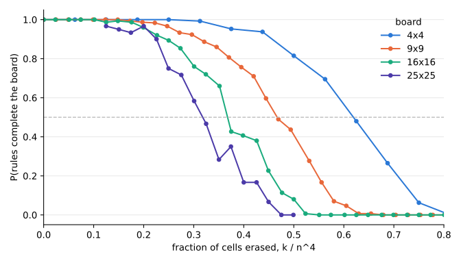
| board | cells \(n^4\) | \(k\) at \(90\%\) success | \(k\) at \(50\%\) success | \(k_{50}/n^4\) |
|---|---|---|---|---|
| \(4\times4\) | 16 | 7 | 9.9 | 0.62 |
| \(9\times9\) | 81 | 25 | 38 | 0.47 |
| \(16\times16\) | 256 | 62 | 94 | 0.37 |
| \(25\times25\) | 625 | 141 | 199 | 0.32 |
Three findings.
(i) Rule R2 barely matters. Success rates with R1 alone and with R1+R2 differ by at most \(12\) percentage points, and by at most \(6\) below \(25\times25\) (largest gap: \(0.05\) versus \(0.17\) on \(25\times25\) at \(k=266\)).
(ii) The rules fail essentially only when the puzzle has more than one completion. For \(9\times9\) boards (\(300\) trials each) a full solution counter found the erased board uniquely completable in \(98\%,\ 80\%,\ 40\%,\ 12\%\) of cases at \(k=20,30,40,46\), and the rules succeeded in exactly the same trials. So the transition measured is the loss of uniqueness, caused by erasing a whole unavoidable set (for example a rectangle \(\{(r,c),(r,c^{\prime}),(r^{\prime},c),(r^{\prime},c^{\prime})\}\) holding \(a,b,b,a\) with \(r,r^{\prime}\) in one band), not weakness of the rules.
(iii) As in Section 8.2, the quantity is a sum of many rare local events. An unavoidable set of size \(s\) is erased with probability about \((k/n^4)^s\), and larger boards contain many more small unavoidable sets, so the \(50\%\) fraction drifts down with \(n\). The \(90\%\to10\%\) window, e.g. \(k\approx 25\) to \(46\) for \(9\times9\), is wide at these sizes: the curves show a threshold but no evidence that it is sharp.
In a square \(n\times n\) grid, each of the \(O(n^2)\) edges is randomly chosen to be present with probability \(p\) and absent with probability \(1-p\). Consider the increasing property that there is a path from the bottom left corner to the top right corner which always goes to the right or up. Show that \(p=1/2\) is a threshold for the property. Is it a sharp threshold?
\(p=1/2\) is a threshold in the sense of Section 8.2, but not a sharp one. Take the grid with vertices \(\{0,\ldots,n\}^2\); a right/up path from \((0,0)\) to \((n,n)\) has \(2n\) edges and is fixed by choosing which \(n\) of its steps go right, so the number \(X\) of present such paths has, using \(\binom{2n}{n}\le 4^n/\sqrt{3n+1}\),
\begin{equation*} E(X)=\binom{2n}{n}p^{2n}\le\frac{(4p^2)^n}{\sqrt{3n+1}}\le\frac{1}{\sqrt{3n+1}}\to0 \qquad(p\le 1/2). \end{equation*}
So for every \(p_1(n)\le 1/2\), in particular whenever \(p_1(n)/(1/2)\to0\), the path almost surely does not exist (first moment method). The other half of the definition, \(p_2(n)/(1/2)\to\infty\), is impossible since \(p_2\le1\), so it holds vacuously (as in Exercise 8.37), and \(1/2\) is a threshold.
Not sharp: sharpness would need the property almost surely for \(p=c/2\) with \(c>1\). But the path needs one of the two edges leaving \((0,0)\) and one of the two edges entering \((n,n)\), four distinct independent edges, so for every constant \(p<1\)
\begin{equation*} \text{Prob(path exists)}\le\big(1-(1-p)^2\big)^2<1 . \end{equation*}
The threshold property seems to be related to uniform distributions. What if we considered other distributions? Consider a model where \(i\) is selected from the set \(\{1,2,\ldots,n\}\) with probability proportional to \(\frac1i\). Is there a threshold for perfect squares? Is there a threshold for arithmetic progressions?
Yes to both: with \(m\) independent draws from \(q_i=1/(iH_n)\), where \(H_n=\sum_{i\le n}1/i=\ln n+O(1)\), both properties have threshold \(m(n)=\ln n\), and neither threshold is sharp. Here “arithmetic progression” means three distinct drawn values \(a,a+d,a+2d\) with \(d\ge1\).
Squares. One draw is a perfect square with probability \(s_n/H_n\), where \(s_n=\sum_{j\le\sqrt n}1/j^2\to\pi^2/6\). Hence
\begin{equation*} \text{Prob(no square)}=\Big(1-\frac{s_n}{H_n}\Big)^{m} \;\to\; \begin{cases}1, & m/\ln n\to0,\\ 0, & m/\ln n\to\infty,\\ e^{-c\pi^2/6}, & m=c\ln n.\end{cases} \end{equation*}
Progressions. If \(m/\ln n\to\infty\) then each of \(1,2,3\) is missed with probability at most \((1-1/(3H_n))^m\le e^{-m/(3H_n)}\to0\), so \(\{1,2,3\}\) is drawn almost surely. If \(m/\ln n\to0\), a union bound over ordered triples of draws gives
\begin{equation*} \begin{aligned} \text{Prob(AP)}&\le m^3\sum_{a,d\ge1}q_aq_{a+d}q_{a+2d} \le\frac{m^3}{H_n^3}\sum_{a\ge1}\frac1a\sum_{d\ge1}\frac{1}{(a+d)^2}\\ &\le\frac{m^3}{H_n^3}\sum_{a\ge1}\frac{1}{a^2}=\frac{\pi^2}{6}\Big(\frac{m}{H_n}\Big)^3\to0 . \end{aligned} \end{equation*}
Not sharp: at \(m=c\ln n\) the numbers of draws equal to \(1,2,3\) converge to independent Poisson\(( c)\), Poisson\((c/2)\), Poisson\((c/3)\) variables, so
\begin{equation*} (1-e^{-c})(1-e^{-c/2})(1-e^{-c/3})\;\le\;\liminf\,\text{Prob(AP)}\;\le\;\frac{\pi^2}{6}c^3 , \end{equation*}
which is bounded away from \(0\) for every \(c>0\) and below \(1\) for small \(c\).
(If instead each \(i\) is included independently with probability \(c/i\), \(0<c\le1\), then \(\text{Prob(square)}\in[c,\,c\pi^2/6]\) and \(\text{Prob(AP)}\in[c^3/6,\,c^3\pi^2/6]\) for all \(n\): no \(n\)-dependent threshold exists at all.)
Modify the proof that every increasing property of \(G(n,p)\) has a threshold to apply to the 3-CNF satisfiability problem.
Let \(F(n,m)\) be the random 3-CNF formula of Section 8.7.2: \(m\) clauses drawn independently and uniformly from the \(8\binom n3\) clauses on \(n\) variables. The increasing property is unsatisfiability, and the threshold is
\begin{equation*} m(n)=\min\{m:\ \text{Prob}(F(n,m)\text{ unsatisfiable})\ge 1/2\}. \end{equation*}
This exists: \(m(n)\ge1\) because the empty formula is satisfiable, and \(m(n)<\infty\) because once all \(8\) sign patterns on \(\{x_1,x_2,x_3\}\) have been drawn the formula is unsatisfiable, which happens with probability tending to \(1\) as \(m\to\infty\). The two ingredients of Section 8.5 become simpler.
(i) Monotonicity, the analogue of Lemma 8.14: the first \(m\) clauses of \(F(n,m^{\prime})\), \(m\le m^{\prime}\), form a copy of \(F(n,m)\), and adding clauses preserves unsatisfiability, so \(\text{Prob}(F(n,m)\text{ unsat})\) is nondecreasing in \(m\).
(ii) Replication, the analogue of (8.3) but now an identity: the conjunction of \(k\) independent copies of \(F(n,m)\) is exactly \(F(n,km)\). An assignment satisfying the conjunction satisfies every copy, so
\begin{equation*} \text{Prob}(F(n,km)\text{ sat})\le\big(\text{Prob}(F(n,m)\text{ sat})\big)^k . \end{equation*}
Below: let \(m_1(n)/m(n)\to0\) and suppose \(\text{Prob}(F(n,m_1)\text{ unsat})\ge\varepsilon\) for \(n\) in an infinite set \(I\). With \(k=\lceil1/\varepsilon\rceil\), (ii) gives \(\text{Prob}(F(n,km_1)\text{ sat})\le(1-\varepsilon)^k\le e^{-1}<1/2\), so \(km_1(n)\ge m(n)\) by minimality, i.e. \(m_1/m\ge1/k\) on \(I\), contradicting \(m_1/m\to0\). So \(F(n,m_1)\) is almost surely satisfiable.
Above: let \(m_2(n)/m(n)\to\infty\) and \(k=\lfloor m_2/m\rfloor\to\infty\). By (i) and (ii), with \(\text{Prob}(F(n,m)\text{ sat})\le1/2\),
\begin{equation*} \text{Prob}(F(n,m_2)\text{ sat})\le\text{Prob}(F(n,km)\text{ sat})\le 2^{-k}\to0 , \end{equation*}
so \(F(n,m_2)\) is almost surely unsatisfiable. Hence \(m(n)\) is a threshold for 3-CNF unsatisfiability, as claimed in Section 8.7.2.
Evaluate \(\left(1-\frac{1}{2^k}\right)^{2^k}\) for \(k=3,5\) and \(7\). How close is it to \(1/e\)?
The values are \(0.343609\), \(0.362055\), \(0.366438\), below \(1/e=0.367879\) by a relative gap of about \(1/(2N)\), \(N=2^k\):
| \(k\) | \(N=2^k\) | \((1-1/N)^N\) | \(1/e-(1-1/N)^N\) | relative gap | \(1/(2N)\) |
|---|---|---|---|---|---|
| 3 | 8 | 0.343609 | 0.024271 | 6.60% | 6.25% |
| 5 | 32 | 0.362055 | 0.005824 | 1.58% | 1.56% |
| 7 | 128 | 0.366438 | 0.001442 | 0.39% | 0.39% |
This follows from
\begin{equation*} N\ln\Big(1-\frac1N\Big)=-1-\frac{1}{2N}-O\Big(\frac{1}{N^2}\Big) \;\Rightarrow\; \Big(1-\frac1N\Big)^N=\frac1e\Big(1-\frac{1}{2N}+O\Big(\frac{1}{N^2}\Big)\Big). \end{equation*}
Exercises 8.43–8.49
For a random 3-CNF formula with \(n\) variables and \(cn\) clauses for some constant \(c\), what is the expected number of satisfying assignments?
The expected number of satisfying assignments is \(2^n(7/8)^{cn}=\bigl(2\,(7/8)^c\bigr)^n\).
By Section 8.7.2 with \(k=3\), a fixed assignment satisfies each of the \(cn\) independent random clauses with probability \(1-2^{-3}\), so by linearity of expectation over the \(2^n\) assignments the number \(X\) of satisfying assignments has
\begin{equation*} E(X)=\sum_{a}\Bigl(1-\tfrac18\Bigr)^{cn}=2^n\Bigl(\tfrac78\Bigr)^{cn}. \end{equation*}
Which of the following variants of the SC algorithm admit a theorem like Theorem 8.20?
(1) Among all clauses of least length, pick the first one in the order in which they appear in the formula. (2) Set the literal appearing in most clauses independent of length to 1.
Variant 1 does, word for word; variant 2 does not. (The exercise’s Theorem 8.20 is the SC theorem, numbered Theorem 8.19 in this draft.)
(1) The proof of Theorem 8.19 uses three facts. Each still holds for variant 1.
- Lemma 8.20. Under deferred decisions, the algorithm may choose the clause to satisfy using anything already revealed. “The first shortest clause in input order” depends only on residual lengths and clause indices, and both are revealed. The clauses are i.i.d., so an index carries no information about unrevealed contents. The literal put into the chosen clause is still a uniformly random unset variable with a fair sign, and every other clause is still decided independently with probability \(l/(n-i)\). So the computation in Lemma 8.20 goes through unchanged: the \(T_i\) are independent and \(\mathrm{Prob}(T_i=t)\le 3/(2(n-2))\).
- Lemma 8.21. Its proof uses only Lemma 8.20 and the fact that every busy step removes one 1- or 2-clause. Variant 1 still always works on a shortest clause, so this holds.
- The final counting. A 0-clause still requires two complementary 1-clauses \(w,\bar w\), because a 1-clause is always served first. During \([t_1,t]\) the literals set true are still independent of these two clauses, so the \(O(n^4(\ln n)^4/n^6)=o(1)\) count is unchanged.
Hence variant 1 succeeds with probability \(1-o(1)\) for \(c<2/3\).
(2) Both ingredients of the proof fail for variant 2.
- Deferred decisions fail. Choosing the most frequent literal requires revealing every clause’s contents, and the chosen literal is by construction over-represented. So no analogue of Lemma 8.20 (independent \(T_i\) with the \(3/(2(n-2))\) bound) is available.
- The length rule is gone. A 1-clause \((w)\) is not served first. It becomes a 0-clause as soon as \(\bar w\) is the most frequent literal, with no complementary 1-clause needed, so the last step of the proof also fails.
Simulation confirms the failure: at \(c=1/2\), variant 2 found a satisfying assignment in \(94\%\) of 100 seeded formulas with \(n=200\), \(70\%\) of 40 with \(n=1000\) and \(20\%\) of 30 with \(n=3000\), a success rate falling with \(n\) rather than tending to 1.
Suppose we have a queue of jobs serviced by one server. There is a total of \(n\) jobs in the system. At time \(t\), each remaining job independently decides to join the queue to be serviced with probability \(p=d/n\), where \(d<1\) is a constant. Each job has a processing time of 1 and at each time the server services one job, if the queue is nonempty. Show that with high probability, no job waits more than \(\Omega(\ln n)\) time to be serviced once it joins the queue.
With \(\kappa=d-1-\ln d>0\) and \(\ell=\lceil (3/\kappa)\ln n\rceil\), with probability \(1-O(\ln n/n^2)\) no job waits \(\ell\) or more steps, so every wait is \(O(\ln n)\). (The printed \(\Omega(\ln n)\) should read \(O(\ln n)\).)
At time \(t=1,2,\dots\) the arrivals \(A_t\) join the queue, and then the server serves one job if the queue is nonempty. Let \(Q_t\) be the queue length after service, so \(Q_0=0\) and \(Q_t=\max(Q_{t-1}+A_t-1,0)\). Couple the process with i.i.d. coins \(B_{t,j}\sim\mathrm{Bernoulli}(d/n)\), \(1\le j\le n\): job \(j\), if it has not yet joined, joins at time \(t\) exactly when \(B_{t,j}=1\). Then \(A_t\le\sum_j B_{t,j}\). For every \(r\) the window sum \(S_r=\sum_{t=r+1}^{r+\ell}\sum_j B_{t,j}\) is distributed as \(\mathrm{Bin}(n\ell,d/n)\), with mean \(m=d\ell\).
Suppose a job joins at time \(t_0\) and is still unserved after time \(t_0+\ell-1\). Then \(Q_t\ge 1\) for \(t\in[t_0,t_0+\ell-1]\). Let \(r=\max\{t<t_0:Q_t=0\}\). Then \(Q_t\ge1\) on \((r,t_0+\ell-1]\), so on that range \(Q_t=Q_{t-1}+A_t-1\). Since \(r+\ell\le t_0+\ell-1\),
\begin{equation*} 1\le Q_{r+\ell}=\sum_{t=r+1}^{r+\ell}A_t-\ell\le S_r-\ell . \end{equation*}
Apply Theorem 12.3 with \(1+\delta=1/d\), so that \((1+\delta)m=\ell\):
\begin{equation*} \begin{aligned} \mathrm{Prob}(S_r>\ell) &<\Bigl(\frac{e^{\delta}}{(1+\delta)^{1+\delta}}\Bigr)^{m} =\exp\bigl(d\ell(\tfrac1d-1)-\ell\ln\tfrac1d\bigr)\\ &=e^{-\kappa\ell}\le n^{-3}. \end{aligned} \end{equation*}
Here \(\kappa>0\) because \(\ln d<d-1\) for \(0<d<1\).
Let \(T=\lceil (3/d)\,n\ln n\rceil\). A given job is still outside the queue after time \(T\) with probability \((1-d/n)^T\le e^{-dT/n}\le n^{-3}\). So all jobs have joined by time \(T\) with probability at least \(1-n^{-2}\). On that event every job has \(t_0\le T\), so \(r<T\). A union bound over \(r\in\{0,\dots,T-1\}\) gives
\begin{equation*} \begin{aligned} \mathrm{Prob}(\text{some job waits}\ge\ell) &\le n^{-2}+T\,n^{-3}\\ &=O\Bigl(\frac{\ln n}{n^{2}}\Bigr)\to 0 . \end{aligned} \end{equation*}
Consider \(G(n,p)\). Show that there is a threshold (not necessarily sharp) for 2-colorability at \(p=1/n\). In particular, first show that for \(p=d/n\) with \(d<1\), with high probability \(G(n,p)\) is acyclic, so it is bipartite and hence 2-colorable. Next, when \(pn\to\infty\), the expected number of triangles goes to infinity. Show that in that case, there is a triangle almost surely and therefore almost surely the graph is not 2-colorable.
\(p=1/n\) is a threshold: if \(pn\to 0\) the graph is almost surely acyclic, hence 2-colorable, and if \(pn\to\infty\) it almost surely contains a triangle, hence is not 2-colorable. The first half as printed is false for fixed \(d<1\). There the number of cycles converges to a Poisson variable with mean \(\lambda(d)=\tfrac12\ln\tfrac1{1-d}-\tfrac d2-\tfrac{d^2}4>0\), so \(\mathrm{Prob}(\text{acyclic})\to e^{-\lambda(d)}<1\); at \(d=0.9\), 400 seeded samples with \(n=3000\) gave \(0.62\) against \(e^{-\lambda}=0.61\). This is why the book calls the threshold in Theorem 8.9 not sharp. So we prove the intended statement, with \(p=o(1/n)\).
(i) Suppose \(pn\to0\). Let \(x\) be the number of cycles. The proof of Theorem 8.9 gives \(E(x)\le 2(np)^3\to0\) (valid once \(np<1/2\)), so \(\mathrm{Prob}(x\ge1)\le E(x)\to 0\) by the first moment method. An acyclic graph is a forest, so it is bipartite and therefore 2-colorable.
(ii) Suppose \(pn\to\infty\). Let \(x=\sum_{ijk}\Delta_{ijk}\) count triangles. Then \(E(x)=\binom n3p^3\ge (np)^3/12\) for \(n\ge6\), which tends to \(\infty\). In \(E(x^2)\), the ordered pairs of triangles split into three kinds.
- Pairs sharing at most one vertex share no edge, so they are independent and contribute at most \(E(x)^2\).
- Pairs sharing one edge span 4 vertices. There are \(\binom n4\cdot 6\cdot 2\) such pairs, each present with probability \(p^5\), so they contribute at most \(n^4p^5/2\).
- Identical pairs contribute \(E(x)\).
Hence
\begin{equation*} \frac{\mathrm{Var}(x)}{E(x)^2}\le\frac{1}{E(x)}+\frac{n^4p^5/2}{E(x)^2} \le\frac{12}{(np)^3}+\frac{72}{n^2p}\to0 , \end{equation*}
because \(np\to\infty\) forces \(n^2p\to\infty\). By Theorem 8.3 (whose hypothesis \(E(x)>0\) holds), \(x>0\) almost surely. A triangle is an odd cycle, so the graph is almost surely not 2-colorable.
A vertex cover of size \(k\) for a graph is a set of \(k\) vertices such that one end of each edge is in the set. Experimentally play with the following problem. For \(G(20,\tfrac12)\), for what value of \(k\) is there a vertex cover of size \(k\)?
A vertex cover of size \(k\) exists exactly when \(k\ge\tau(G)=20-\alpha(G)\). For \(G(20,\tfrac12)\) the minimum cover size \(\tau\) is usually 15, often 14, and rarely 13 or 16. So \(k\ge16\) works for essentially every graph and \(k\le12\) essentially never.
The identity holds because \(S\) is a vertex cover iff \(V\setminus S\) is an independent set, and any superset of a cover is still a cover. The program computes \(\alpha\) exactly as the clique number of the complement for 1000 seeded samples.
import networkx as nx, numpy as np
from collections import Counter
rng = np.random.default_rng(0)
mins = []
for _ in range(1000):
    G = nx.gnp_random_graph(20, 0.5, seed=int(rng.integers(1 << 30)))
    alpha = max(len(c) for c in nx.find_cliques(nx.complement(G)))
    mins.append(20 - alpha)          # minimum vertex cover = n - alpha
print(sorted(Counter(mins).items()), np.mean(mins))
The minimum cover sizes it reports are:
| \(k\) | 13 | 14 | 15 | 16 |
|---|---|---|---|---|
| fraction of graphs with \(\tau(G)=k\) | 0.015 | 0.343 | 0.602 | 0.040 |
| fraction with a cover of size \(k\) | 0.015 | 0.358 | 0.960 | 1.000 |
The mean is \(14.67\).
The first moment method (Section 8.2) explains these numbers. The expected number of independent sets of size \(a\) is \(\binom{20}{a}2^{-\binom a2}\), which equals \(15.1\), \(1.18\) and \(0.037\) for \(a=5,6,7\). So \(\alpha\ge7\), that is \(\tau\le13\), has probability at most \(0.037\) (observed \(0.015\)). Sets of size 5 are plentiful (observed \(\alpha\ge5\), i.e. \(\tau\le15\), in \(96\%\) of graphs), and size 6 sits right at the transition (observed in \(36\%\)).
Construct an example of a formula which is satisfiable, but the SC heuristic fails to find a satisfying assignment.
Take \(f=(x_1\vee x_2)(\bar x_1\vee x_2)(x_1\vee\bar x_2)\). It is satisfied only by \(x_1=x_2=1\), and SC fails on it with probability \(1/3\).
All three clauses are shortest, so SC picks one of the 6 (clause, literal) pairs uniformly at random.
- (i) It picks \(\bar x_1\) in clause 2. Clauses 1 and 3 shrink to \((x_2)\) and \((\bar x_2)\). Whichever of them SC satisfies next turns the other into a 0-clause: failure.
- (ii) It picks \(\bar x_2\) in clause 3. Clauses 1 and 2 shrink to \((x_1)\) and \((\bar x_1)\): failure, by the same argument.
- (iii) It picks any of the other four pairs, which set \(x_1=1\) or \(x_2=1\). The single remaining clause becomes the unit clause of the other variable, and SC sets it true: success.
So \(\mathrm{Prob}(\text{SC fails})=2/6=1/3\).
In \(G(n,p)\), let \(x_k\) be the number of connected components of size \(k\). Using \(x_k\), write down the probability that a randomly chosen vertex is in a connected component of size \(k\). Also write down the expected size of the connected component containing a randomly chosen vertex.
The probability is \(k x_k/n\), and the expected size is \(\tfrac1n\sum_k k^2x_k\).
For a fixed graph, the components of size \(k\) contain exactly \(k x_k\) of the \(n\) vertices. So for a uniformly random vertex \(v\) with component \(C(v)\),
\begin{equation*} \mathrm{Prob}\bigl(|C(v)|=k\bigr)=\frac{k\,x_k}{n},\qquad E\,|C(v)|=\sum_{k=1}^{n}k\cdot\frac{k\,x_k}{n}=\frac1n\sum_{k=1}^{n}k^2x_k . \end{equation*}
Averaging also over \(G(n,p)\) replaces \(x_k\) by \(E(x_k)\), which Lemma 8.10 bounds:
\begin{equation*} \begin{aligned} \mathrm{Prob}\bigl(|C(v)|=k\bigr)&=\frac{k\,E(x_k)}{n},\qquad E\,|C(v)|=\frac1n\sum_{k=1}^{n}k^2E(x_k),\\ E(x_k)&\le\binom nk k^{k-2}p^{k-1}(1-p)^{kn-k^2}. \end{aligned} \end{equation*}
Exercises 8.50–8.56
Describe several methods of generating a random graph with a given degree distribution. Describe differences in the graphs generated by the different methods.
Five standard methods, given a degree sequence \(d_1,\dots,d_n\) with \(\sum_i d_i\) even:
(1) Configuration (pairing) model. Give vertex \(i\) exactly \(d_i\) half-edges (“stubs”) and pair all \(\sum_i d_i\) stubs by a uniformly random perfect matching. Every vertex gets exactly its degree, but the result is a multigraph. Conditioned on being simple, it is uniform over simple graphs with this degree sequence. This is the model of Section 8.8, and it is the one the Molloy-Reed criterion \(\sum_i i(i-2)\lambda_i>0\) of Section 8.8.1 describes. Rejecting non-simple outcomes keeps uniformity but becomes hopeless when \(\max_i d_i\) is large. Erasing loops and repeated edges instead lowers the degrees of the hubs. (2) Expected-degree (Chung-Lu) model. Join \(i\) and \(j\) independently with probability \(p_{ij}=\min(1,d_id_j/\sum_k d_k)\). This is the \(G(n,p)\) of Section 8.1 with nonuniform \(p\). Edges are independent, so it is easy to analyse, but \(d_i\) is only the mean degree: the realised degrees are roughly Poisson\((d_i)\), and some vertices come out isolated. (3) Havel-Hakimi. Repeatedly join the vertex of largest residual degree to the vertices of next-largest residual degree. This is deterministic, not random. Hubs link to hubs, giving a dense rich club full of triangles, while the low-degree vertices pair off among themselves into many small components. (4) Edge-switching Markov chain. Start from any realisation (for example Havel-Hakimi) and repeatedly replace edges \(\{a,b\},\{c,d\}\) by \(\{a,d\},\{c,b\}\) when that creates no loop or multi-edge. Degrees are preserved exactly, and the stationary distribution is uniform over simple realisations. The only cost is mixing time. (5) Growth models (Section 8.9). Preferential attachment fixes only the shape of the distribution: a power law, with exponent set by the model. A vertex’s degree is correlated with its age, the oldest vertices are the hubs, and with one edge per new vertex the graph is a tree.
Power-law sequence (\(n=2000\), \(d_i=\lfloor 2(1+X_i)\rfloor\) with \(X_i\) Pareto of index \(1.5\), so \(\mathrm{Prob}(d_i=k)\sim k^{-2.5}\), capped at \(200\); mean degree \(5.47\); networkx, seed 0):
| method | degree sequence exact? | assortativity | transitivity | components |
|---|---|---|---|---|
| configuration | yes, with 22 loops and 202 repeated edges | \(-0.094\) (erased) | \(0.034\) | 1 |
| Chung-Lu | for 23% of vertices; 161 isolated | \(-0.062\) | \(0.058\) | 165 |
| Havel-Hakimi | yes, simple | \(+0.048\) | \(0.352\) | 470 |
| Havel-Hakimi + swaps | yes, simple | \(-0.141\) | \(0.034\) | 1 |
The methods that sample (approximately) uniformly (configuration, Chung-Lu, swap chain) produce statistically similar graphs. These are locally tree-like, mildly disassortative, and have vanishing clustering. The deterministic and growth constructions add structure that the degree sequence does not determine: clustering and fragmentation for Havel-Hakimi, age-degree correlation and tree structure for preferential attachment.
Consider generating a random graph adding one edge at a time. Let \(n(i,t)\) be the number of components of size \(i\) at time \(t\).
\begin{equation*} \begin{aligned} n(1,1)&=n\\ n(1,t)&=0\qquad t>1\\ n(i,t)&=n(i,t-1)+\sum \frac{j(i-j)}{n^2}\,n(j,t-1)\,n(i-j,t-1)-\frac{2i}{n}\,n(i) \end{aligned} \end{equation*}
Compute \(n(i,t)\) for a number of values of \(i\) and \(t\). What is the behavior? What is the sum of \(n(i,t)\) for fixed \(t\) and all \(i\)? Can you write a generating function for \(n(i,t)\)?
The behaviour is that of Erdos-Renyi with mean degree \(s=2t/n\). Below the critical time \(t=n/2\) the component sizes follow the Borel law and there are exactly \(n-t\) components. Above it, the mass that leaves the finite sizes is the giant component.
Conventions. The printed initial condition “\(n(1,t)=0\), \(t>1\)” should read “\(n(i,1)=0\), \(i>1\)” (all vertices start isolated); we shift time so that \(t\) counts the edges added, i.e. \(n(1,0)=n\) and \(n(i,0)=0\) for \(i\ge2\). The sum runs over \(1\le j\le i-1\), and the final \(n(i)\) means \(n(i,t-1)\). The recursion is the mean-field (expected) count. The new edge joins a size-\(j\) component to a size-\((i-j)\) component with probability \(j(i-j)n(j)n(i-j)/n^2\), and it touches a given size-\(i\) component with probability about \(2i/n\). Edges falling inside a single component are ignored.
Computation (\(n=1000\), sizes truncated at \(i\le n/2\) so that \(2i/n\le1\); an untruncated run goes negative and diverges shortly after \(t=n/2\)):
import numpy as np
n, I = 1000, 500
N = np.zeros(I+1); N[1] = n; j = np.arange(I+1)
for t in range(1, 801):
    gain = np.convolve(j*N, j*N)[:I+1] / n**2
    N = N + gain - 2*j*N/n
    if t in (100, 250, 400, 500, 600, 800):
        print(t, N.sum(), n - (j*N).sum(), N[1], N[2])
Results, with means over 200 actual union-find simulations shown after the slash:
| \(t\) | \(\sum_i n(i,t)\) | \(n(1,t)\) | \(n(2,t)\) | mass in sizes \(>n/2\) | \(n\theta\) |
|---|---|---|---|---|---|
| 100 | 900.0 / 900.1 | 818.6 / 818.5 | 67.3 / 67.9 | 0 | 0 |
| 250 | 750.0 / 750.3 | 606.2 / 605.9 | 92.2 / 93.4 | 0 | 0 |
| 400 | 600.0 / 600.7 | 449.0 / 449.3 | 80.9 / 81.7 | 0 | 0 |
| 600 | 403.5 / 405.7 | 300.8 / 300.7 | 54.5 / 55.4 | 312.0 | 313.7 |
| 800 | 255.1 / 257.1 | 201.6 / 201.8 | 32.6 / 33.5 | 642.4 | 642.0 |
Here \(\theta\) is the root in \((0,1)\) of \(1-\theta=e^{-s\theta}\). The recursion tracks the true process closely. Isolated vertices decay like \(ne^{-2t/n}\), and small components first grow and then are absorbed. From \(t\approx n/2\) on, mass escapes to a giant component of the size given by the branching-process prediction for \(G(n,s/n)\). The simulated largest component has \(640.5\) vertices at \(t=800\).
Sum. Let \(M_1=\sum_i i\,n(i,t-1)\) and \(M_2=\sum_i i^2n(i,t-1)\), with \(M_1=n\) at \(t=0\). Summing the recursion over \(i\) (the convolution factorises) gives
\begin{equation*} \begin{aligned} \sum_i i\,n(i,t)&=M_1+\frac{2M_1M_2}{n^2}-\frac{2M_2}{n}=M_1=n,\\ \sum_i n(i,t)&=\sum_i n(i,t-1)+\frac{M_1^2}{n^2}-\frac{2M_1}{n}=\sum_i n(i,t-1)-1, \end{aligned} \end{equation*}
so \(\sum_i n(i,t)=n-t\): each edge merges two components. This holds exactly until \(t\approx n/2\). After that the giant component absorbs mass, and the edges that close cycles keep the true count above \(n-t\), as the table shows.
Generating function. Put \(F_t(x)=\frac1n\sum_i i\,n(i,t)x^i\), so \(F_0(x)=x\) and \(F_t(1)=1\). Multiplying the recursion by \(ix^i/n\) and summing gives
\begin{equation*} F_t(x)=F_{t-1}(x)+\frac{2}{n}\,x\,F_{t-1}^{\prime}(x)\bigl(F_{t-1}(x)-1\bigr). \end{equation*}
With \(\tau=t/n\) this becomes \(\partial_\tau F=2x\,\partial_xF\,(F-1)\). Its solution is given implicitly by
\begin{equation*} F(x,t)=x\,e^{(2t/n)(F(x,t)-1)} \end{equation*}
(check by implicit differentiation: both sides equal \(2F(F-1)/(1-sF)\)). By Lagrange inversion,
\begin{equation*} n(i,t)\approx n\,\frac{i^{\,i-2}}{i!}\Bigl(\frac{2t}{n}\Bigr)^{i-1}e^{-2ti/n}, \end{equation*}
the Borel distribution, which agrees with every tabulated \(n(1,t)\) and \(n(2,t)\) to within \(0.4\). For \(s=2t/n\le1\) we have \(F(1)=1\). For \(s>1\), \(F(1)=1-\theta\) is the fraction of vertices in finite components.
The global clustering coefficient of a graph is defined as follows. Let \(d_v\) be the degree of vertex \(v\) and let \(e_v\) be the number of edges connecting pairs of vertices that are adjacent to vertex \(v\). The global clustering coefficient \(c\) is given by
\begin{equation*} c=\sum_v \frac{2e_v}{d_v(d_v-1)}. \end{equation*}
In a social network, for example, it measures what fraction of pairs of friends of each person are themselves friends. If many are, the clustering coefficient is high. What is \(c\) for a random graph with \(p=\frac dn\) in the limit as \(n\) goes to infinity? For a denser graph? Compare this value to that for some social network.
In \(G(n,d/n)\) we have \(E( c)=\frac dn\bigl(1-(1+d)e^{-d}\bigr)(1+o(1))\to0\). In a dense \(G(n,p)\), \(c\to p\). Real social networks have \(c\) far above their edge density.
The printed \(c\) is a sum, and a sum grows with \(n\). We take the intended average \(c=\frac1n\sum_v c_v\), where \(c_v=2e_v/(d_v(d_v-1))\) and \(c_v=0\) when \(d_v<2\).
Condition on the neighbourhood \(N(v)\) with \(|N(v)|=k\ge2\). The \(\binom k2\) pairs inside \(N(v)\) are disjoint from the edges at \(v\), so in \(G(n,p)\) each is present independently with probability \(p\). Hence \(E(e_v\mid N(v))=p\binom k2\), and
\begin{equation*} \begin{aligned} E( c)=E(c_v)&=p\,\mathrm{Prob}(d_v\ge2)\\ &=\frac dn\Bigl(1-\bigl(1-\tfrac dn\bigr)^{n-1} -\tfrac{(n-1)d}{n}\bigl(1-\tfrac dn\bigr)^{n-2}\Bigr). \end{aligned} \end{equation*}
Since \(d_v\to\mathrm{Poisson}(d)\) (Section 8.1.1), this is \(\frac dn(1-(1+d)e^{-d})(1+o(1))\). Because \(c\ge0\), Markov’s inequality gives \(c\to0\) in probability. Simulation agrees: averaged over 10 seeds with \(d=5\), \(c=0.00233\) for \(n=2000\) (formula \(0.00240\)) and \(c=0.000271\) for \(n=20000\) (formula \(0.000240\)).
For a denser graph with \(p\) constant, \(E(c_v)=p\,(1-o(1))\). Each \(c_v\to p\) in probability (since \(d_v\sim pn\to\infty\) and \(e_v\sim\mathrm{Bin}(\binom{d_v}2,p)\)), and \(0\le c_v\le1\), so \(E|c-p|\le E|c_v-p|\to0\). Thus \(c\to p\); in general \(c\approx\) edge density. A simulation of \(G(400,0.3)\) (seed 0) gave \(c=0.302\).
Social networks (computed in networkx):
| network | \(n\) | edges | density \(p\) | \(c\) |
|---|---|---|---|---|
| Zachary karate club | 34 | 78 | 0.139 | 0.571 |
| Les Miserables co-appearance | 77 | 254 | 0.087 | 0.573 |
For a much larger example, Watts and Strogatz (1998) report \(c=0.79\) for the film-actor network, against \(0.00027\) for a random graph with the same \(n\) and mean degree. A random graph cannot reproduce the clustering of a social network. Its \(c\) equals the density, which tends to \(0\) for sparse graphs, while friends of friends in a real social network are friends with constant probability.
Consider a structured graph, such as a grid or cycle, and gradually add edges or reroute edges at random. Let \(L\) be the average distance between all pairs of vertices in a graph and let \(C\) be the ratio of triangles to connected sets of three vertices. Plot \(L\) and \(C\) as a function of the randomness introduced.
A small amount of rewiring collapses \(L\) while \(C\) stays put. At \(p\approx0.014\), \(L\) has fallen to about 15% of its lattice value while \(C\) is still about 91% of its lattice value. This is the small-world regime.
A plain cycle or grid has no triangles (\(C\equiv0\)), so the structured graph is the ring lattice: \(n=1000\) vertices on a cycle, each joined to its \(5\) nearest neighbours on each side (\(k=10\)). Each edge is rerouted to a uniformly random endpoint with probability \(p\) (networkx’s connected Watts-Strogatz model). \(C\) is the number of triangles divided by the number of connected 3-vertex sets, which equals \(T/(P-2T)\), where \(T\) is the number of triangles and \(P=\sum_v\binom{d_v}2\).
import numpy as np, networkx as nx
def C3(G):
    T = sum(nx.triangles(G).values())/3
    P = sum(d*(d-1)/2 for _, d in G.degree())
    return T/(P - 2*T)
for p in np.logspace(-4, 0, 14):
    Gs = [nx.connected_watts_strogatz_graph(1000, 10, p, seed=s) for s in range(3)]
    L = np.mean([nx.average_shortest_path_length(G) for G in Gs])
    C = np.mean([C3(G) for G in Gs])
    print(p, L, C)
At \(p=0\) the lattice has \(L(0)=50.45\) and \(C(0)=0.4\). Means over three seeds:
| \(p\) | \(10^{-4}\) | \(8.4\cdot10^{-4}\) | \(0.0035\) | \(0.014\) | \(0.059\) | \(0.24\) | \(1\) |
|---|---|---|---|---|---|---|---|
| \(L\) | 48.53 | 26.96 | 14.24 | 7.50 | 5.00 | 3.75 | 3.27 |
| \(C\) | 0.400 | 0.398 | 0.392 | 0.366 | 0.289 | 0.120 | 0.003 |
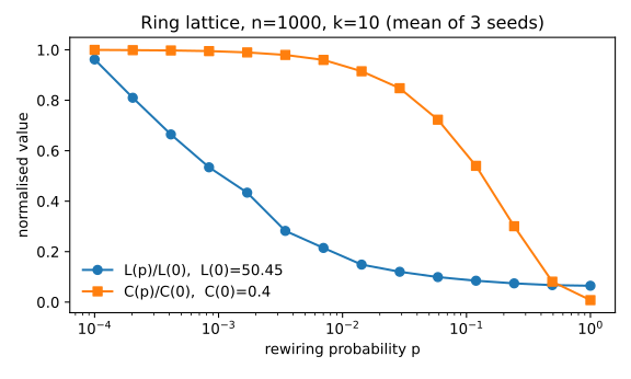
\(L\) drops as soon as the number of shortcuts, \(5000p\), is of order one: about 17 shortcuts at \(p=0.0035\) already cut \(L\) by 72%. Each shortcut joins two random far-apart points, and these random edges give the logarithmic diameter of Theorem 8.13 and of the \(r=0\) small-world graph in Section 8.10. At \(p=1\), \(L=3.27\), compared with \(\ln n/\ln k=3.0\) for a random graph of the same degree.
\(C\) falls only when a constant fraction of each vertex’s local edges has been rewired, because a triangle survives as long as its three local edges are untouched. At \(p=1\) the graph is essentially \(G(n,k/n)\), and \(C=0.0031\) matches \(T/P\approx\frac13\cdot\frac kn=0.0033\), a third of the clustering \(c\approx p\) of Exercise 8.52.
Consider an \(n\times n\) grid in the plane. (1) Prove that for any vertex \(u\), there are at least \(k\) vertices at distance \(k\) for \(1\le k\le n/2\). (2) Prove that for any vertex \(u\), there are at most \(4k\) vertices at distance \(k\). (3) Prove that for one half of the pairs of points, the distance between them is at least \(n/4\).
Take vertices \((x,y)\) with \(1\le x,y\le n\). Grid distance is \(d((a,b),(x,y))=|x-a|+|y-b|\), and \(u=(a,b)\).
(1) Choose a horizontal direction \(\sigma\in\{\pm1\}\) with room \(\max(a-1,n-a)\ge\lceil (n-1)/2\rceil=\lfloor n/2\rfloor\ge k\), and a vertical direction \(\tau\) in the same way. The \(k\) points
\begin{equation*} (a+\sigma i,\;b+\tau(k-i)),\qquad i=1,\dots,k, \end{equation*}
are distinct (different \(i\) give different first coordinates). They lie in the grid (\(0\le i,k-i\le k\)), and each is at distance \(i+(k-i)=k\) from \(u\).
(2) Even in all of \(\mathbb Z^2\), the points at distance \(k\ge1\) are the solutions of \(|\Delta x|+|\Delta y|=k\). For each \(\Delta x\in\{-k,\dots,k\}\) there are two choices \(\Delta y=\pm(k-|\Delta x|)\), except one choice when \(|\Delta x|=k\). That gives \(2(2k+1)-2=4k\) points, and the grid contains at most these.
(3) In fact at least \(3/4\) of the pairs of distinct points are at distance at least \(n/4\). Let \(m\) be the largest integer below \(n/4\), so \(4m\le n-1\). By part 2, each \(u\) has at most \(\sum_{k=1}^m 4k=2m(m+1)\) points \(v\ne u\) with \(d(u,v)<n/4\). The fraction of the \(n^2-1\) partners \(v\ne u\) that are this close is therefore
\begin{equation*} \begin{aligned} \frac{2m(m+1)}{n^2-1} &\le\frac{2\cdot\frac{n-1}4\cdot\frac{n+3}4}{(n-1)(n+1)}\\ &=\frac{n+3}{8(n+1)}\le\frac14 . \end{aligned} \end{equation*}
The last step uses \(n+3\le 2(n+1)\). Averaging over \(u\), at most a quarter of all pairs are at distance less than \(n/4\).
Recall the definition of a small-world graph in Section 8.10. Show that in a small-world graph with \(r\le2\), that there exist short paths with high probability. The proof for \(r=0\) is in the text.
For \(0\le r<2\), with high probability every ordered pair has a directed path of length \(O(\ln n)\). For \(r=2\), every pair has one of length \(O(\ln^3 n)\). Both are polylogarithmic, against grid distances of order \(n\). We take \(r\ge0\), which is the family of Section 8.10.
Write \(N=n^2\) and \(P(u\to v)=d^{-r}(u,v)/c_r(u)\).
(i) Case \(0\le r<2\): a uniform floor. We have \(d(u,v)<2n\), and by Exercise 8.54(2) there are at most \(4k\) vertices at distance \(k\). Also \(\sum_{k=1}^{2n}k^{1-r}\le 2(2n)^{2-r}/(2-r)\): for \(r\le1\) bound each term by \((2n)^{1-r}\); for \(1<r<2\) compare with \(1+\int_1^{2n}x^{1-r}dx\). Therefore
\begin{equation*} \begin{aligned} c_r(u)&\le\sum_{k=1}^{2n}4k\cdot k^{-r}\le\frac{8(2n)^{2-r}}{2-r},\\ P(u\to v)&\ge\frac{(2n)^{-r}(2-r)}{8(2n)^{2-r}}=\frac{\alpha}{N},\\ \alpha&=\frac{2-r}{32}. \end{aligned} \end{equation*}
Coupling: let \(\beta=\alpha(N-1)/N\ge\alpha/2\). Then \(P(u\to\cdot)=\beta\,U_u+(1-\beta)Q_u\), where \(U_u\) is uniform on \(V\setminus\{u\}\) and \(Q_u\ge0\) is a probability vector. So each \(u\) can flip a \(\beta\)-coin and, on heads, draw its long edge from \(U_u\). Deleting the tails edges leaves a subgraph \(H\): the grid plus, independently for each \(u\) with probability \(\beta\), one uniform long edge. Distances in the small-world graph are at most those in \(H\). The text’s \(r=0\) case is \(\beta=1\). Lemma \((\ast)\) below makes that argument quantitative for any constant \(\beta>0\). It applies here with \(a=\frac12\), \(A=5\), using Exercise 8.54: \(|B(v,\rho)|\ge1+\sum_{k\le\rho}k\ge\rho^2/2\) and \(|B(v,\rho)|\le1+\sum_{k\le\rho}4k\le5\rho^2\).
Lemma \((\ast)\). Let \(\Gamma\) be an undirected graph on \(N=n^2\) vertices with \(a\rho^2\le|B(v,\rho)|\le A\rho^2\) for all \(v\) and \(1\le\rho\le n/2\). Independently, let each \(u\) have, with probability \(\beta\), a directed edge to a uniform vertex of \(V\setminus\{u\}\). Then with probability \(1-O(1/n)\) every ordered pair is joined by a directed path of length \(O(\ln n)\).
Proof. Fix constants: \(\rho_0\) with \(\beta a\rho_0^2\ge4\), \(B=A\rho_0^2\), \(K=72/\beta\) and \(\gamma=1/(32B^2)\).
Growth. Fix \(s\) and let \(A_0=E_0=B(s,\rho_1)\) with \(\rho_1=\lceil\sqrt{K\ln n/a}\,\rceil\), so \(|A_0|\ge K\ln n\). In round \(j\), process the vertices \(u\in A_j\) one at a time. Reveal \(u\)’s coin and endpoint \(w_u\). Call \(u\) good if the coin is heads and \(B(w_u,\rho_0)\) misses \(X\), the union of \(E_j\) and the balls already added this round. Put \(B(w_u,\rho_0)\) into \(A_{j+1}\) when \(u\) is good, and set \(E_{j+1}=E_j\cup A_{j+1}\). By induction every vertex of \(A_j\) is reachable from \(s\) in at most \(\rho_1+j(\rho_0+1)\) steps, and every \(u\in A_j\) is fresh: its coin and endpoint have not been revealed yet. Since \(|X|\le(1+B)|E_j|\), the endpoints \(w\) with \(B(w,\rho_0)\cap X\ne\emptyset\) lie in \(\bigcup_{x\in X}B(x,\rho_0)\), a set of size at most \(2B^2|E_j|\). So while \(|E_j|\le(N-1)/(8B^2)\), each \(u\) is good with conditional probability at least \(3\beta/4\). Hence the number of good vertices dominates \(\mathrm{Bin}(|A_j|,3\beta/4)\). By Chernoff, with probability at least \(1-e^{-\beta|A_j|/24}\) at least \(\beta|A_j|/2\) vertices are good. The balls of good vertices are disjoint, so
\begin{equation*} |A_{j+1}|\ge\frac{\beta|A_j|}2\,a\rho_0^2\ge2|A_j| . \end{equation*}
Let \(J\) be the first round with \(|E_J|>(N-1)/(8B^2)\). Doubling gives \(|A_j|\ge2^jK\ln n\), so \(J\le\log_2N\). It also gives \(|E_J|\le2|A_J|\), so \(|A_J|\ge\gamma N\). The growth fails with probability at most
\begin{equation*} \sum_{j\ge0}n^{-\beta K2^j/24}\le2n^{-3}, \end{equation*}
which is \(O(n^{-1})\) after a union bound over the \(n^2\) sources.
Connection. Fix \(t\) and let \(\rho_2=\lceil\sqrt{K^{\prime}\ln n/a}\,\rceil\) with \(K^{\prime}=10/(\gamma\beta)\). Conditional on the exploration, the \(|A_J|\ge\gamma N\) fresh vertices independently send an edge into \(B(t,\rho_2)\), each with probability at least \(\beta K^{\prime}\ln n/(2N)\). All of them miss with probability at most
\begin{equation*} e^{-\gamma\beta K^{\prime}\ln n/2}=n^{-5}, \end{equation*}
which is \(O(n^{-1})\) after a union bound over the \(n^4\) pairs. Otherwise \(s\to u\in A_J\to w\in B(t,\rho_2)\to t\) is a path of length at most \(\rho_1+J(\rho_0+1)+1+\rho_2=O(\ln n)\). \(\square\)
(ii) Case \(r=2\). Use the greedy walk of Section 8.10: always move to the neighbour, grid or long-distance, that is closest to \(t\). Distance to \(t\) strictly decreases, so no vertex is visited twice and each long edge examined is fresh. When the current distance \(k^{\prime}\) lies in \((k/2,k]\), the text’s computation shows that the long edge lands in \(B(t,k^{\prime}/2)\subseteq B(t,k/2)\) with probability at least \(c/\ln n\). This uses the \(\Omega(k^{\prime\,2})\) such vertices, each at distance at most \(3k^{\prime}/2\), and \(c_2(u)=O(\ln n)\). So a halving phase lasts more than \(M=\lceil(6/c)\ln^2n\rceil\) steps with probability at most \((1-c/\ln n)^M\le n^{-6}\). There are at most \(\log_2(2n)+1\) phases, so a union bound over phases and \(n^4\) pairs leaves failure probability \(O(n^{-2}\ln n)\). Every pair is then joined by a path of length at most \(M(\log_2 2n+1)=O(\ln^3n)\).
Change the small worlds graph as follows. Start with a \(n\times n\) grid where each vertex has one long-distance edge to a vertex chosen uniformly at random. These are exactly like the long-distance edges for \(r=0\). Instead of having grid edges, we have some other graph with the property that for each vertex, there are \(\Theta(t^2)\) vertices at distance \(t\) from the vertex for \(t\le n\). Show that, almost surely, the diameter is \(O(\ln n)\).
This is Lemma \((\ast)\) of Exercise 8.55 with \(\beta=1\).
As printed, the hypothesis is impossible: \(\Theta(t^2)\) vertices at each distance \(t\le n\) would give \(\sum_{t\le n}\Theta(t^2)=\Theta(n^3)\) vertices, but there are only \(n^2\). The intended grid-like condition is that the ball of radius \(t\) has \(\Theta(t^2)\) vertices. That is, there are constants \(0<a\le A\) such that the undirected local graph \(\Gamma\) satisfies
\begin{equation*} a t^2\le|B_\Gamma(v,t)|\le At^2,\qquad 1\le t\le n/2, \end{equation*}
for every vertex \(v\). (Only radii \(t=O(\sqrt{\ln n})\) are used.)
Lemma \((\ast)\) needs exactly the following:
- the two-sided ball bound for \(\Gamma\);
- undirected local edges, so that \(B(t,\rho_2)\) reaches \(t\) within \(\rho_2\) steps and \(w\in B(x,\rho_0)\iff x\in B(w,\rho_0)\);
- independent long edges with \(P(u\to v)\ge\beta/(N-1)\).
With uniform long-distance edges the last condition holds with \(\beta=1\), and no coupling is needed. The lemma then gives that, with probability \(1-O(1/n)\), every ordered pair \((s,t)\) is joined by a directed path of length
\begin{equation*} \rho_1+J(\rho_0+1)+1+\rho_2=O(\sqrt{\ln n})+O(\log_2 n^2)+O(\sqrt{\ln n})=O(\ln n). \end{equation*}
Hence the diameter is \(O(\ln n)\) almost surely.
Exercises 8.57–8.60
Consider an \(n\)-node directed graph with two random out-edges from each node. For two vertices \(s\) and \(t\) chosen at random, prove that with high probability there exists a path of length at most \(O(\ln n)\) from \(s\) to \(t\).
As printed the claim is false, and the intended statement is: with high probability, either no path from \(s\) to \(t\) exists, or one of length \(O(\ln n)\) does. To see the failure, note the in-degree of \(t\) is \(\text{Bin}(2n,1/n)\), so \(\text{Prob}(\text{in-deg}(t)=0)=(1-1/n)^{2n}\to e^{-2}\approx 0.135\), and then \(t\) cannot be reached at all.
Write \(e_1(u),e_2(u)\) for the out-edges of \(u\), which are i.i.d. uniform on \(V\). Fix \(C=16\), and set \(K=C\ln n\), \(m=3C\ln n\) and \(M=mK=O(\ln^2 n)\).
Backward exploration. Let \(L_j\) be the set of vertices at distance exactly \(j\) to \(t\), with \(\ell_j=|L_j|\) and \(B_j=L_0\cup\dots\cup L_j\). To find \(L_{j+1}\) we ask each \(u\notin B_j\) whether \(e_1(u)\) or \(e_2(u)\) lies in \(L_j\). Up to this point the history only tells us that the edges of such a \(u\) avoid \(B_{j-1}\), so its edges are i.i.d. uniform on \(V\setminus B_{j-1}\). Hence
\begin{equation*} \ell_{j+1}\sim \text{Bin}\Big(n-|B_j|,\;1-\big(1-\tfrac{\ell_j}{n-|B_{j-1}|}\big)^2\Big). \end{equation*}
While \(|B_j|\le M\) and \(\ell_j\le K\), this law is within total variation \(O(KM/n)\) of \(\text{Poisson}(2\ell_j)\). That is Le Cam’s bound \(d_{TV}(\text{Bin}(N,p),\text{Poi}(Np))\le p\), plus \(|Np-2\ell_j|=O(\ell_j M/n)\). So the layer sizes can be coupled with the generations \(Z_j\) of a Poisson(2) branching process (Section 8.6), with failure probability \(O(mKM/n)=o(1)\).
That process has \(f(x)=e^{2(x-1)}\) and extinction probability \(q\approx0.203\) (Theorem 8.17), and \(Z_m\) has generating function \(f_m\), the \(m\)-th iterate of \(f\). Since \(f\) maps \([q,\tfrac12]\) into itself and \(f^{\prime}\) is increasing, \(f^{\prime}\le f^{\prime}(\tfrac12)=2/e\) there and \(f^{\prime}\le f^{\prime}(q)=2q<2/e\) on \([0,q]\). Therefore
\begin{equation*} \begin{aligned} \text{Prob}(1\le Z_m<K)&\le 2^{K}\big(f_m(\tfrac12)-f_m(0)\big)\\ &\le 2^{K}\Big[(\tfrac2e)^m(\tfrac12-q)+(2q)^m q\Big]\\ &\le 2\,e^{C\ln n\,(\ln 2+3\ln(2/e))}=2\,n^{-0.228\,C}\to0 . \end{aligned} \end{equation*}
Meeting. Suppose \(t\) is reachable from \(s\) with \(d(s,t)>m\). Then every layer \(L_1,\dots,L_m\) is nonempty. By the bound above, outside an \(o(1)\) event some \(\ell_j\ge K\) with \(j\le m\); stop the backward exploration at the first such \(j\). If \(s\in B_j\) we are done. Otherwise, explore forward from \(s\) by BFS. Every draw from a vertex \(u\notin B_j\) is a fresh uniform point of \(V\setminus B_{j-1}\), and hitting \(B_j\) gives a path of length at most \((\text{forward depth})+1+m\).
(i) For depth \(d_0=\lceil 2\log_2\ln n\rceil\), the first \(\le 4\ln^2 n\) draws collide with each other or with \(B_j\) with probability at most \(4\ln^2 n\,(4\ln^2n+M)/(n-M)=o(1)\). So the BFS tree is binary and its frontier has \(F\ge\ln^2 n\) vertices.
(ii) Let \(D\) be the set discovered so far. While \(|D|\le n/8\) and \(F\le|D|\), each of the \(2F\) frontier draws is new with conditional probability at least \(1-(3n/8+M)/(n-M)\ge 0.6\). So the number of new vertices dominates \(\text{Bin}(2F,0.6)\), of mean \(1.2F\), and by Theorem 12.4 with \(\gamma=1/12\),
\begin{equation*} \text{Prob}\big(\text{new frontier}<1.1F\big)\le e^{-(1/12)^2(1.2F)/2}=e^{-F/240}\le e^{-\ln^2 n/240}. \end{equation*}
So after \(h=d_0+\log_{1.1}n+1=O(\ln n)\) levels we have \(|D|\ge n/8\), which gives at least \(n/8-1\) draws, each conditionally landing in \(L_j\) with probability at least \(K/n\).
(iii) Hence
\begin{equation*} \text{Prob}(\text{no draw hits }L_j)\le(1-K/n)^{n/8-1}\le e\cdot e^{-K/8}=e\,n^{-2}. \end{equation*}
Adding up the failure events,
\begin{equation*} \text{Prob}\big(m+h+1<d(s,t)<\infty\big)=o(1), \end{equation*}
so with high probability, whenever \(t\) is reachable from \(s\) it is reachable by a path of length \(O(\ln n)\). \(\blacksquare\)
Explore the concept of small world by experimentally determining the answers to the following questions: (1) How many edges are needed to disconnect a small world graph? By disconnect we mean at least two pieces each of reasonable size. Is this connected to the emergence of a giant component? (2) How does the diameter of a graph consisting of a cycle change as one adds a few random long-distance edges?
In the \(r=0\) small world you have to cut \(\Theta(N)\) edges to split it into two large pieces, between a quarter and a half of its long-distance edges, against \(\Theta(\sqrt N)\) for the bare grid. Removing random edges does not split it into two large pieces except near the percolation threshold: it keeps one giant component until the giant itself dissolves. Adding \(k\) random chords to an \(N\)-cycle cuts the diameter from \(N/2\) to about \((N/k)\ln k\).
The graph is Kleinberg’s model of Section 8.10: a \(40\times40\) grid (\(N=1600\)) plus one long-distance edge per vertex, ending at \(v\) with probability proportional to \(d(u,v)^{-r}\), treated as undirected. The program below (seed 58) does three things. It upper-bounds the minimum bisection with the best of 5 Kernighan-Lin runs. It lower-bounds it by \(\lambda_2(L)\,N/4\), because a bisection \((A,B)\) cuts at least \(\lambda_2|A||B|/N\) edges. It also keeps each edge independently with probability \(p\) and records the two largest components.
import numpy as np, networkx as nx, matplotlib; matplotlib.use('Agg'); import matplotlib.pyplot as plt
from networkx.algorithms.community import kernighan_lin_bisection as kl
rng = np.random.default_rng(58); n = 40; xy = np.array([(i, j) for i in range(n) for j in range(n)])
def kleinberg(r):                       # n x n grid + one long edge per vertex, Prob ~ d^-r
    G = nx.convert_node_labels_to_integers(nx.grid_2d_graph(n, n), ordering='sorted')
    for u in range(n*n):
        d = np.abs(xy - xy[u]).sum(1); w = np.where(d > 0, d + 0.0, np.inf)**(-r)
        G.add_edge(u, rng.choice(n*n, p=w/w.sum()))
    return G
for r in [None, 0, 2, 4]:               # None = bare grid
    G = kleinberg(r) if r is not None else nx.convert_node_labels_to_integers(nx.grid_2d_graph(n, n))
    lam = np.sort(np.linalg.eigvalsh(nx.laplacian_matrix(G).toarray().astype(float)))[1]
    cut = min(nx.cut_size(G, *kl(G, seed=s)) for s in range(5)); E = np.array(G.edges()); comp = []
    for p in [0.2, 0.25, 0.3, 0.5]:
        H = nx.Graph(list(E[rng.random(len(E)) < p])); H.add_nodes_from(G)
        comp.append(sorted(map(len, nx.connected_components(H)))[-2:][::-1])
    print(r, len(E), round(lam*n*n/4), cut, comp)
N, ks = 1000, [0, 1, 2, 5, 10, 20, 50, 100, 200, 500, 1000]; diam = []
for k in ks:
    ds = []
    for _ in range(5):
        C = nx.cycle_graph(N); C.add_edges_from(rng.integers(0, N, (k, 2))); ds.append(nx.diameter(C))
    diam.append(np.mean(ds))
plt.figure(figsize=(5, 3.5)); plt.loglog(np.array(ks[1:]), diam[1:], 'o-', label='cycle + k chords')
plt.loglog(ks[2:], [N/k*np.log(k) for k in ks[2:]], '--', label='(N/k) ln k')
plt.xlabel('k random chords (N = 1000)'); plt.ylabel('diameter'); plt.legend(); plt.tight_layout()
for e in ['svg', 'pdf']: plt.savefig('fds-ch08-cyclediam.' + e)
(1) In the next table, “largest, second” gives the two largest components after keeping each edge with probability \(p\).
| graph | edges | bisection \(\ge\) | bisection \(\le\) (KL) | \(p=0.2\) | \(p=0.25\) | \(p=0.3\) | \(p=0.5\) |
|---|---|---|---|---|---|---|---|
| grid only | 3120 | 2 | 46 | 16, 12 | 22, 17 | 37, 36 | 467, 302 |
| \(r=0\) | 4713 | 412 | 816 | 130, 87 | 822, 16 | 1212, 9 | 1543, 2 |
| \(r=2\) | 4278 | 83 | 232 | 40, 31 | 217, 168 | 939, 27 | 1517, 5 |
| \(r=4\) | 3360 | 3 | 50 | 15, 14 | 28, 27 | 46, 43 | 1263, 49 |
The grid splits in half by cutting \(n=40\) edges (KL finds 46). For \(r=0\) any split into halves must cut at least 412 edges, of roughly \(1600\) long ones: the long edges make an expander, like \(G(n,p)\), so a balanced cut costs \(\Theta(N)\). For \(r=2\) the long edges are mostly local and the cut drops to between 83 and 232, and for \(r=4\) the graph behaves like the grid.
Random deletion is a different matter and ties to Section 8.3. For \(r=0\) the giant appears between \(p=0.2\) and \(p=0.25\). That matches the tree-like estimate \(p_c\approx E(d)/E(d(d-1))\approx 6/31\approx0.19\), with degree \(d\approx 5+\text{Poisson}(1)\) (Section 8.8). Once the giant exists the second component stays tiny (16, 9, 2), just as \(G(n,p)\) has only one giant component. So removing random edges does not produce two large pieces: the graph keeps one giant plus dust until the giant itself disappears. Two large pieces appear only near the critical point, as in the grid and \(r=4\) at \(p=0.5\) (467 and 302, since the grid’s bond-percolation threshold is exactly \(1/2\)). Disconnecting into reasonable-size pieces therefore needs a chosen cut, and the small-world shortcuts raise its cost from \(\Theta(\sqrt N)\) to \(\Theta(N)\).
(2) For the cycle \(C_{1000}\) with \(k\) uniformly random chords, averaged over 5 graphs:
| \(k\) | 0 | 1 | 2 | 5 | 10 | 20 | 50 | 100 | 200 | 500 | 1000 |
|---|---|---|---|---|---|---|---|---|---|---|---|
| diameter | 500 | 500 | 411.4 | 316.2 | 233.6 | 130 | 75.8 | 43.6 | 27 | 15 | 10 |
A single chord does not help, because the original cycle still has antipodal pairs at distance \(N/2\). After that the diameter falls quickly. For \(10\le k\le200\) it tracks \((N/k)\ln k\) within about 15%. The chords cut the cycle into arcs of length about \(N/k\), and their \(2k\) endpoints form a sparse random graph of diameter \(O(\ln k)\), as in Theorem 8.13. Once \(k\) is comparable to \(N\) the graph is a random cubic-like graph with diameter \(O(\ln N)\): 10 at \(k=N\).
In the small world model with \(r<2\), would it help if the algorithm could look at edges at any node at a cost of one for each node looked at?
No, not in any essential way. Even with free choice of which nodes to probe, polylogarithmic cost finds a polylog-length \(s\)-\(t\) path with probability \(o(1)\). In general,
\begin{equation*} \text{cost}\cdot(\text{path length})^2 \gtrsim n^{2-r}. \end{equation*}
Let \(Q\) be the number of nodes probed, \(L=n^{\delta}\) the target length, and \(B\) the ball of grid radius \(L\) around \(t\). Then \(|B|\le 4L^2\). An \(s\)-\(t\) path with fewer than \(L\) edges, where \(s\notin B\) (true with probability \(1-O(L^2/n^2)\)), must use a long-distance edge that ends in \(B\). Otherwise it enters \(B\) through its boundary and needs at least \(L\) more grid steps. The algorithm can only output such an edge if it has probed the edge’s tail.
Each probed node \(u\) reveals one long-distance edge, which is independent of every other node’s edge, so adaptivity does not matter. Since \(c_r(u)=\Omega(n^{2-r})\) for every \(u\) (Section 8.10), each probe lands in \(B\) with probability at most \(|B|\cdot O(n^{r-2})\). Therefore
\begin{equation*} \begin{aligned} \text{Prob}(\text{a path of length}<L\text{ is found}) &\le Q\cdot 4L^2\cdot O(n^{r-2})+O(L^2/n^2)\\ &=O\big(Q\,n^{2\delta-(2-r)}\big)+o(1). \end{aligned} \end{equation*}
With \(Q\) polylogarithmic and \(\delta=(2-r)/3\), this is \(O(Q\,n^{-(2-r)/3})=o(1)\). So paths of length \(n^{(2-r)/3}\) are still out of reach, much as for the local algorithm of Section 8.10, whose bound is \(n^{(2-r)/4}\). Finding a path of length \(L\) needs \(Q=\Omega(n^{2-r}/L^2)\) probes, which is \(n^{2-r-o(1)}\) when \(L\) is polylog.
The bound is attained for \(r=0\). Probe the nodes of a BFS from \(s\), in which \(\Omega(n^2)\) nodes lie within \(O(\ln n)\) steps (end of Section 8.10). Stop at the first probed node whose long edge ends within \(\rho\) of \(t\), then walk at most \(\rho\) grid steps. Each probe succeeds independently with probability at least \(\rho^2/(2n^2)\), so \(Q=O(n^2\ln n/\rho^2)\) probes suffice with high probability, giving a path of length \(O(\ln n+\rho)\).
Make a list of the ten most interesting things you learned about random graphs.
(1) Phase transitions are universal. Every increasing property of \(G(n,p)\) has a threshold (Theorem 8.15). Many thresholds are sharp: isolated vertices disappear at \(\ln n/n\) (Theorem 8.6), and diameter two appears at \(\sqrt{2\ln n/n}\) (Theorem 8.5). (2) The first and second moment methods (Theorem 8.3) decide most thresholds. \(E(x)\to0\) kills a property, and \(\mathrm{Var}(x)=o(E^2(x))\) forces it. (3) At \(p=1/n\) the graph changes abruptly. Below it, components have size \(O(\ln n)\) and are almost all trees. Above it, a single giant component of linear size appears (Section 8.3), and cycles appear at the same point (Theorem 8.9). (4) There is never more than one giant component. Two linear-size components would almost surely be joined by an edge. (5) Connectivity arrives exactly when the last isolated vertex disappears (Theorem 8.11). Just before that, the only obstacles are single vertices. (6) Above \(c\ln n/n\) the diameter is \(O(\ln n)\) (Theorem 8.13), because neighbourhoods grow geometrically until they must intersect. (7) Branching processes explain the giant component. The extinction probability is the smallest root of \(f(x)=x\) (Theorem 8.17), and the expected number of children per node decides survival. (8) Degree distribution alone predicts a giant component. The Molloy-Reed condition \(\sum_i i(i-2)\lambda_i>0\) (Section 8.8) recovers \(p=1/n\) for \(G(n,p)\). (9) Growth matters. A graph grown without preferential attachment gets its giant component at \(\delta=1/8\), while a static graph with the same degree distribution needs \(\delta=1/4\): older vertices form a core. Preferential attachment gives the power law \(p(d)=2\delta^2/d^3\) (Section 8.9). (10) Short paths are not the same as findable paths. In Kleinberg’s grid, short paths exist for every \(r<2\), but a local algorithm finds them only at \(r=2\), where greedy routing takes \(O(\ln^3 n)\) steps (Section 8.10). In the same spirit, the shortest-clause heuristic solves random 3-SAT with \(cn\) clauses when \(c<2/3\) (Theorem 8.19), well below the satisfiability threshold.
Topic Models, NMF, Hidden Markov Models, and Graphical Models
Exercises 9.1–9.7
Find a nonnegative factorization of the matrix
\begin{equation*} A=\begin{pmatrix} 4 & 6 & 5\\ 1 & 2 & 3\\ 7 & 10 & 7\\ 6 & 8 & 4\\ 6 & 10 & 11 \end{pmatrix}. \end{equation*}
Indicate the steps in your method and show the intermediate results.
\begin{equation*} A=\begin{pmatrix} 1 & \tfrac12\\ 1 & 0\\ 1 & 1\\ 0 & 1\\ 3 & \tfrac12 \end{pmatrix} \begin{pmatrix} 1 & 2 & 3\\ 6 & 8 & 4 \end{pmatrix}. \end{equation*}
We follow the anchor-term method of Section 9.4: find the rows of \(A\) that are not nonnegative combinations of the other rows, make them the rows of \(C\), and read off \(B\).
(i) Rank. Row reduction gives \(\operatorname{rank} A=2\) (rows 2 and 4 are independent and the other rows lie in their span, as (iii) shows).
(ii) Extreme rows. Write \(a_i\) for row \(i\). All the rows lie in a 2-dimensional space, so the cone they generate is spanned by the two rows with the extreme values of the ratio \(a_{i3}/a_{i1}\); a nonnegative combination of rows has its ratio between the smallest and the largest ratio of the rows used:
| row \(i\) | 1 | 2 | 3 | 4 | 5 |
|---|---|---|---|---|---|
| \(a_{i3}/a_{i1}\) | \(5/4\) | \(3\) | \(1\) | \(2/3\) | \(11/6\) |
Row 2 has the unique maximum and row 4 the unique minimum, so neither is a nonnegative combination of the other rows. These are the anchor rows, and we take \(C=\begin{pmatrix} a_2\\ a_4\end{pmatrix}\).
(iii) Coefficients. Solving \(a_i=x\,a_2+y\,a_4\) for each remaining row gives
\begin{equation*} \begin{aligned} (4,6,5)&=1\cdot(1,2,3)+\tfrac12(6,8,4),\\ (7,10,7)&=1\cdot(1,2,3)+1\cdot(6,8,4),\\ (6,10,11)&=3\cdot(1,2,3)+\tfrac12(6,8,4), \end{aligned} \end{equation*}
with all coefficients nonnegative. Together with \(a_2=1\cdot a_2\) and \(a_4=1\cdot a_4\), these coefficient pairs are the rows of \(B\), and that is the factorization above. Both factors are nonnegative and \(BC=A\) (Check!).
Find a nonnegative factorization of each of the following matrices.
\begin{equation*} (1)\ \begin{pmatrix} 10 & 9 & 15 & 14 & 13\\ 2 & 1 & 3 & 3 & 1\\ 8 & 7 & 13 & 11 & 11\\ 7 & 5 & 11 & 10 & 7\\ 5 & 5 & 11 & 6 & 11\\ 1 & 1 & 3 & 1 & 3\\ 2 & 2 & 2 & ? & 2 \end{pmatrix} \end{equation*}
\begin{equation*} (2)\ \begin{pmatrix} 5 & 5 & 10 & 14 & 17\\ 2 & 2 & 4 & 4 & 6\\ 1 & 1 & 2 & 4 & 4\\ 1 & 1 & 2 & 2 & 3\\ 3 & 3 & 6 & 8 & 10\\ 5 & 5 & 10 & 16 & 18\\ 2 & 2 & 4 & 6 & 7 \end{pmatrix} \end{equation*}
\begin{equation*} (3)\ \begin{pmatrix} 4 & 4 & 3 & 3 & 1 & 3 & 4 & 3\\ 13 & 16 & 13 & 10 & 5 & 13 & 14 & 10\\ 15 & 24 & 21 & 12 & 9 & 21 & 18 & 12\\ 7 & 16 & 15 & 6 & 7 & 15 & 10 & 6\\ 1 & 4 & 4 & 1 & 2 & 4 & 2 & 1\\ 5 & 8 & 7 & 4 & 3 & 7 & 6 & 4\\ 3 & 12 & 12 & 3 & 6 & 12 & 6 & 3 \end{pmatrix} \end{equation*}
\begin{equation*} (4)\ \begin{pmatrix} 1 & 1 & 3 & 4 & 4 & 4 & 1\\ 9 & 9 & 9 & 12 & 9 & 9 & 3\\ 6 & 6 & 12 & 16 & 15 & 15 & 4\\ 3 & 3 & 3 & 4 & 3 & 3 & 1 \end{pmatrix} \end{equation*}
(The entry in row 7, column 4 of matrix (1) is missing from the printed text.)
The factorizations are displayed below; as in Section 9.4, the rows of \(C\) are the rows \(a_i\) of \(A\) that are not nonnegative combinations of the other rows, and row \(i\) of \(B\) expresses \(a_i\) in terms of them. For the rank-2 matrices (2)-(4), a nonnegative combination of rows has its ratio \(a_{iq}/a_{ip}\) between the smallest and largest ratio of the rows used, so the generating rows are the ones with the extreme ratios.
(1) The missing entry is taken to be \(3\), which is the only value that makes the matrix have rank 3 (with \(0\) there the rank is 4); flagged as a misprint. With \(a_7=(2,2,2,3,2)\):
\begin{equation*} \begin{pmatrix} 10 & 9 & 15 & 14 & 13\\ 2 & 1 & 3 & 3 & 1\\ 8 & 7 & 13 & 11 & 11\\ 7 & 5 & 11 & 10 & 7\\ 5 & 5 & 11 & 6 & 11\\ 1 & 1 & 3 & 1 & 3\\ 2 & 2 & 2 & 3 & 2 \end{pmatrix} =\begin{pmatrix} 1&2&3\\ 1&0&0\\ 1&2&2\\ 2&1&1\\ 0&3&1\\ 0&1&0\\ 0&0&1 \end{pmatrix} \begin{pmatrix} 2&1&3&3&1\\ 1&1&3&1&3\\ 2&2&2&3&2 \end{pmatrix}. \end{equation*}
The rows of \(C\) are \(a_2,a_6,a_7\). None of them is a nonnegative combination of the other rows, because each has a linear functional that separates it from the rest:
\begin{equation*} \begin{aligned} 2a_{i5}-a_{i1}&=(16,\,0,\,14,\,7,\,17,\,5,\,2) &&\text{zero only at } a_2,\\ 3a_{i1}-a_{i3}&=(15,\,3,\,11,\,10,\,4,\,0,\,4) &&\text{zero only at } a_6,\\ a_{i3}-a_{i4}&=(1,\,0,\,2,\,1,\,5,\,2,\,-1) &&\text{negative only at } a_7. \end{aligned} \end{equation*}
The remaining rows decompose as \(a_1=a_2+2a_6+3a_7\), \(a_3=a_2+2a_6+2a_7\), \(a_4=2a_2+a_6+a_7\) and \(a_5=3a_6+a_7\).
(2) Here the rank is 2. The ratios \(a_{i4}/a_{i1}\) are \((\tfrac{14}5,2,4,2,\tfrac83,\tfrac{16}5,3)\), so the extreme rows are \(a_3\) (the maximum) and \(a_4\) (the minimum; \(a_2=2a_4\)):
\begin{equation*} \begin{pmatrix} 5 & 5 & 10 & 14 & 17\\ 2 & 2 & 4 & 4 & 6\\ 1 & 1 & 2 & 4 & 4\\ 1 & 1 & 2 & 2 & 3\\ 3 & 3 & 6 & 8 & 10\\ 5 & 5 & 10 & 16 & 18\\ 2 & 2 & 4 & 6 & 7 \end{pmatrix} =\begin{pmatrix} 2&3\\ 0&2\\ 1&0\\ 0&1\\ 1&2\\ 3&2\\ 1&1 \end{pmatrix} \begin{pmatrix} 1&1&2&4&4\\ 1&1&2&2&3 \end{pmatrix}. \end{equation*}
(3) Here the rank is 2. The ratios \(a_{i2}/a_{i1}\) are \((1,\tfrac{16}{13},\tfrac85,\tfrac{16}7,4,\tfrac85,4)\), so the extreme rows are \(a_1\) (the minimum) and \(a_5\) (the maximum; \(a_7=3a_5\)):
\begin{equation*} \begin{pmatrix} 4 & 4 & 3 & 3 & 1 & 3 & 4 & 3\\ 13 & 16 & 13 & 10 & 5 & 13 & 14 & 10\\ 15 & 24 & 21 & 12 & 9 & 21 & 18 & 12\\ 7 & 16 & 15 & 6 & 7 & 15 & 10 & 6\\ 1 & 4 & 4 & 1 & 2 & 4 & 2 & 1\\ 5 & 8 & 7 & 4 & 3 & 7 & 6 & 4\\ 3 & 12 & 12 & 3 & 6 & 12 & 6 & 3 \end{pmatrix} =\begin{pmatrix} 1&0\\ 3&1\\ 3&3\\ 1&3\\ 0&1\\ 1&1\\ 0&3 \end{pmatrix} \begin{pmatrix} 4&4&3&3&1&3&4&3\\ 1&4&4&1&2&4&2&1 \end{pmatrix}. \end{equation*}
(4) Here the rank is 2. The ratios \(a_{i3}/a_{i1}\) are \((3,1,2,1)\), so the extreme rows are \(a_1\) (the maximum) and \(a_4\) (the minimum; \(a_2=3a_4\)):
\begin{equation*} \begin{pmatrix} 1 & 1 & 3 & 4 & 4 & 4 & 1\\ 9 & 9 & 9 & 12 & 9 & 9 & 3\\ 6 & 6 & 12 & 16 & 15 & 15 & 4\\ 3 & 3 & 3 & 4 & 3 & 3 & 1 \end{pmatrix} =\begin{pmatrix} 1&0\\ 0&3\\ 3&1\\ 0&1 \end{pmatrix} \begin{pmatrix} 1&1&3&4&4&4&1\\ 3&3&3&4&3&3&1 \end{pmatrix}. \end{equation*}
All factors are nonnegative and every product equals its matrix (Check!).
Consider the matrix \(A\) that is the product of nonnegative matrices \(B\) and \(C\):
\begin{equation*} \begin{pmatrix} 12 & 22 & 41 & 35\\ 19 & 20 & 13 & 48\\ 11 & 14 & 16 & 29\\ 14 & 16 & 14 & 36 \end{pmatrix} =\begin{pmatrix} 10 & 1\\ 1 & 9\\ 3 & 4\\ 2 & 6 \end{pmatrix} \begin{pmatrix} 1 & 2 & 4 & 3\\ 2 & 2 & 1 & 5 \end{pmatrix}. \end{equation*}
Which rows of \(A\) are approximate positive linear combinations of other rows of \(A\)? Find an approximate nonnegative factorization of \(A\).
Rows 3 and 4. In fact they are exact positive combinations of rows 1 and 2:
\begin{equation*} \begin{aligned} a_3&=\tfrac{23}{89}\,a_1+\tfrac{37}{89}\,a_2,\\ a_4&=\tfrac{12}{89}\,a_1+\tfrac{58}{89}\,a_2 . \end{aligned} \end{equation*}
To see this, note that \(a_i=b_iC\), where \(b_i\) is row \(i\) of \(B\), and that the two rows of \(C\) are linearly independent. Hence \(a_i\) is a nonnegative combination of other rows of \(A\) if and only if \(b_i\) is the same combination of the corresponding rows of \(B\). The ratios \(b_{i2}/b_{i1}\) are \((\tfrac1{10},\,9,\,\tfrac43,\,3)\). A positive combination has its ratio strictly between the extreme ratios of the rows used, so:
- \(b_1\) (the minimum ratio) and \(b_2\) (the maximum ratio) are not combinations of the other rows;
- \(b_3\) and \(b_4\) are combinations of \(b_1\) and \(b_2\), namely \((3,4)=\tfrac{23}{89}(10,1)+\tfrac{37}{89}(1,9)\) and \((2,6)=\tfrac{12}{89}(10,1)+\tfrac{58}{89}(1,9)\).
Following Section 9.4, we keep the extreme rows as the new \(C\). This gives a nonnegative factorization that is in fact exact:
\begin{equation*} A=\begin{pmatrix} 1 & 0\\ 0 & 1\\ \tfrac{23}{89} & \tfrac{37}{89}\\ \tfrac{12}{89} & \tfrac{58}{89} \end{pmatrix} \begin{pmatrix} 12 & 22 & 41 & 35\\ 19 & 20 & 13 & 48 \end{pmatrix}. \end{equation*}
Both factors are nonnegative and the product is \(A\) (Check!).
Consider a set of vectors \(S\) in which no vector is a positive linear combination of the other vectors in the set. Given a set \(T\) containing \(S\) along with a number of elements from the convex hull of \(S\), find the vectors in \(S\). Develop an efficient method to find \(S\) from \(T\) which does not require linear programming.
Hint: The points of \(S\) are vertices of the convex hull of \(T\). The Euclidean length of a vector is a convex function and so its maximum over a polytope is attained at one of the vertices. Center the set and find the maximum length vector in \(T\). This will be one element of \(S\).
Repeatedly take the point of \(T\) that is farthest from the span of the points already found (successive projection):
c  = mean of T
t1 = point of T maximising |t - c|          (first vertex)
for every t in T:  u(t) = t - t1
Q  = empty orthonormal list
repeat:
    for every t:  w(t) = u(t) minus its projection onto span(Q)
    t* = point of T maximising |w(t)|
    if |w(t*)| = 0:  stop
    add t* to the found list;  append w(t*)/|w(t*)| to Q
return the found list (t1 and every t*)
Each round costs \(O(|T|\,d)\) with Gram-Schmidt updates, so the total cost is \(O(|S|\,|T|\,d)\), and no linear program is solved. As in Section 9.4, where \(S\) is the set of \(r\) rows of \(C\) and \(A\) has rank \(r\) (Lemma 9.3), we assume that \(S=\{s_1,\dots,s_k\}\) is linearly, hence affinely, independent. Every \(t\in T\) is then \(t=\sum_s\lambda_s(t)\,s\) with unique convex weights \(\lambda(t)\).
First vertex. Suppose \(t\in T\) maximises \(f(x)=|x-c|^2\) but \(t\notin S\). Then \(\lambda(t)\) has at least two positive weights, and strict convexity of \(f\) gives
\begin{equation*} f(t)<\sum_s\lambda_s(t)f(s)\le\max_{s\in S}f(s), \end{equation*}
which contradicts the maximality of \(t\), since \(S\subseteq T\). Hence \(t_1\in S\).
Later rounds. Let \(F\ni t_1\) be the set of vertices found so far and let \(P\) be the orthogonal projection onto \(\mathrm{span}\{s-t_1:s\in F\}^{\perp}\). The vectors \(s-t_1\) for \(s\ne t_1\) are linearly independent, so the vectors \(v_s=P(s-t_1)\) for \(s\notin F\) are linearly independent; in particular each is nonzero. For \(t\in T\),
\begin{equation*} \begin{aligned} |P(t-t_1)|&=\Bigl|\sum_{s\notin F}\lambda_s(t)\,v_s\Bigr| \le\sum_{s\notin F}\lambda_s(t)\,|v_s|\\ &\le\max_{s\notin F}|v_s| . \end{aligned} \end{equation*}
Equality in the triangle inequality forces the \(v_s\) carrying positive weight to be positively parallel. Independent vectors are never parallel, so only one \(v_s\) carries weight, and equality in the last step forces that weight to be \(\lambda_s(t)=1\). So the maximiser is \(t=s\in S\setminus F\), and the maximum is positive while \(F\ne S\). When \(F=S\), every \(P(t-t_1)\) is \(0\) and the loop stops. Therefore the method returns exactly \(S\). \(\blacksquare\)
Define the nonnegative column rank of an \(m\times n\) matrix \(A\) to be the minimum number of vectors in \(m\)-space with the property that every column of \(A\) can be expressed as a nonnegative linear combination of these vectors. (1) Show that the nonnegative column rank of \(A\) is at least the rank of \(A\). (2) Construct a \(3\times n\) matrix whose nonnegative column rank is \(n\). [Hint: Take the plane \(x+y=z=1\) in 3-space; draw a circle in the plane and take \(n\) points on the circle.] (3) Show that the nonnegative column rank need not be the same as the nonnegative row rank. (4) Read/look up a paper of Vavasis showing that the computation of nonnegative rank is NP-hard.
Erratum: read literally (generators any vectors), the quantity is at most \(m\) for \(A\ge0\) (take \(e_1,\dots,e_m\)), so part 2 fails for \(n\ge4\), and with nonnegative generators it is the nonnegative rank \(\min\{r:A=BC,\ B,C\ge0\}\), which is the same for \(A\) and \(A^T\), so part 3 fails; following the anchor setting of Section 9.4, we require the generators to be columns of \(A\) (for rows, rows of \(A\)).
(1) Suppose every column of \(A\) is a nonnegative combination of \(v_1,\dots,v_k\). Then
\begin{equation*} \mathrm{col}(A)\subseteq\mathrm{span}\{v_1,\dots,v_k\},\qquad\text{so}\qquad \operatorname{rank}A\le k . \end{equation*}
(2) Take \(\theta_j=2\pi j/n\) and let column \(j\) of \(A\) be
\begin{equation*} a_j=(1+\cos\theta_j,\ 1+\sin\theta_j,\ 1)^T\ge0,\qquad j=1,\dots,n . \end{equation*}
These are \(n\) points on a circle in the plane \(z=1\) (we read the misprinted hint plane as \(z=1\)). Suppose \(a_j=\sum_{k\ne j}c_ka_k\) with all \(c_k\ge0\). The third coordinate gives \(\sum_kc_k=1\). Write \(u_k=(\cos\theta_k,\sin\theta_k)\) and take the inner product of the first two coordinates with \(u_j\):
\begin{equation*} 1=u_j\cdot u_j=\sum_{k\ne j}c_k\cos(\theta_k-\theta_j)<\sum_{k\ne j}c_k=1 , \end{equation*}
a contradiction. So no column is a nonnegative combination of the others. Every generating set of columns must therefore contain all \(n\) columns, and the nonnegative column rank is \(n\).
(3) Take the matrix of part 2 with \(n\ge4\). Its nonnegative column rank is \(n\), while its nonnegative row rank is at most \(3\), because the 3 rows trivially generate themselves. Hence \(3<n\) and the two ranks differ.
(4) S. A. Vavasis, On the complexity of nonnegative matrix factorization, SIAM J. Optim. 20 (2009) 1364-1377. The paper considers exact NMF: given \(A\) of rank \(k\), decide whether \(A=BC\) with \(B,C\ge0\) and inner dimension \(k\), that is, whether the nonnegative rank equals the rank. It shows this problem is equivalent to the intermediate simplex problem: given a polytope \(P\) and a point set \(Q\subseteq P\), find a simplex \(\Delta\) with \(Q\subseteq\Delta\subseteq P\). It then reduces 3-SAT to the intermediate simplex problem. So computing the nonnegative rank is NP-hard when \(k\) is part of the input (for constant \(k\) it is polynomial by Lemma 9.3).
What happens to the Topic Modeling problem when \(m\), the number of words in a document, goes to infinity? Argue that the Idealized Topic Modeling problem of Section 9.2 is easy to solve when \(m\) goes to infinity.
As \(m\to\infty\) the noise \(N=A-BC\) in (9.3) vanishes, and Topic Modeling becomes exact Nonnegative Matrix Factorization \(A=BC\) (Section 9.3 calls NMF exactly this limiting case). Given \(C\), the entry \(a_{ij}\) is the average of \(m\) independent indicators \(1\{x_t=i\}\), each with mean \(p_{ij}\) (Definition 9.1). By the strong law of large numbers,
\begin{equation*} a_{ij}\xrightarrow[m\to\infty]{\text{a.s.}}p_{ij}=(BC)_{ij}\quad\text{for all } i\le d,\ j\le n, \end{equation*}
and the convergence is simultaneous because there are finitely many pairs. Hence \(A\to P=BC\).
In the idealized model of Section 9.2, column \(j\) of \(C\) is the unit vector \(e_{l(j)}\), so in the limit
\begin{equation*} A(:,j)=B\,e_{l(j)}=B(:,l(j)) . \end{equation*}
Separability makes the supports \(S_l\) of the columns of \(B\) disjoint and nonempty, so the \(r\) topic columns are pairwise distinct. The problem is therefore solved by grouping identical columns, for example by sorting or hashing them in \(O(nd\log n)\) time:
- the groups are the clusters \(T_1,\dots,T_r\) of Definition 9.2, with no misclustering;
- the \(r\) distinct columns are exactly the columns of \(B\);
- \(C\) is the indicator matrix of the groups.
Suppose \(\mathbf y=(y_1,y_2,\dots,y_r)\) is jointly distributed according to the Dirichlet distribution with parameter \(\mu=1/r\). Show that the expected value of \(\max_{l=1}^r y_l\) is greater than \(0.1\). [Hint: Lemma 9.6]
In fact \(E\max_l y_l\ge\frac2\pi\,2^{-3/2}>0.22\). The hint’s Lemma 9.6 should be Lemmas 9.4-9.5, and the marginal density printed in Lemma 9.4 is missing a \(-1\) in the exponent of \(1-y\); we use the correct marginal \(y_1\sim\mathrm{Beta}(\mu,(r-1)\mu)\). This follows from the representation \(y_l=G_l/\sum_kG_k\) with \(G_l\) i.i.d. \(\mathrm{Gamma}(\mu)\), which gives \(y_1=G_1/(G_1+G^{\prime})\) with \(G^{\prime}\sim\mathrm{Gamma}((r-1)\mu)\) independent of \(G_1\).
If \(r=1\), then \(\max_l y_l=1\). Let \(r\ge2\). At most one \(y_l\) can exceed \(\tfrac12\), so the events \(\{y_l>\tfrac12\}\) are disjoint, as in the proof of Lemma 9.5. Using \(\Gamma(\tfrac1r)\Gamma(1-\tfrac1r)=\pi/\sin(\pi/r)\),
\begin{equation*} \begin{aligned} E\max_l y_l&\ge E\bigl[\max_l y_l\,;\,\max_l y_l>\tfrac12\bigr]\\ &=\sum_{l=1}^rE\bigl[y_l\,;\,y_l>\tfrac12\bigr]\\ &=r\,\frac{\sin(\pi/r)}{\pi}\int_{1/2}^1y\cdot y^{\frac1r-1}(1-y)^{-\frac1r}\,dy\\ &\ge\frac{\sin(\pi/r)}{\pi/r}\cdot\Bigl(\tfrac12\Bigr)^{1/r}\cdot\tfrac12 \ \ge\ \frac2\pi\cdot\Bigl(\tfrac12\Bigr)^{3/2}\approx0.225>0.1 . \end{aligned} \end{equation*}
In the third line we used \(y^{1/r}\ge(\tfrac12)^{1/r}\ge(\tfrac12)^{1/2}\) and \((1-y)^{-1/r}\ge1\) on \([\tfrac12,1]\), together with \(\sin x/x\ge 2/\pi\) for \(x=\pi/r\in(0,\pi/2]\). \(\blacksquare\)
Exercises 9.8–9.13
Suppose there are \(s\) documents in a collection which are all nearly pure for a particular topic, i.e., in each of these documents that topic has weight at least \(1-\delta\). Suppose someone finds and hands to you these documents. Then their average is an approximation to the topic vector. In terms of \(s\), \(m\) and \(\delta\) compute an upper bound on the error of approximation.
The mean-square error is at most \(2\delta^2+\frac{1}{sm}\): if \(\bar a=\frac1s\sum_{j=1}^s A(:,j)\) and \(b_l=B(:,l)\) is the topic vector, then
\begin{equation*} \mathbf{E}\,\|\bar a-b_l\|_2^2\le 2\delta^2+\frac{1}{sm}, \qquad\text{so}\qquad \|\bar a-b_l\|_2\le\sqrt{\frac{2\delta^2+1/(sm)}{\eta}} \ \text{ with probability}\ \ge 1-\eta . \end{equation*}
Condition on the topic mixtures \(C(:,j)\) of the \(s\) documents, so \(p_j=BC(:,j)\) is fixed, and put \(\bar p=\frac1s\sum_j p_j\). Split the error into bias plus noise, \(\bar a-b_l=(\bar p-b_l)+(\bar a-\bar p)\).
Bias. Every column of \(B\) is a probability vector, so \(\|b_{l^{\prime}}\|_2\le\|b_{l^{\prime}}\|_1=1\) and \(b_{l^{\prime}}\cdot b_l\ge0\), which gives \(\|b_{l^{\prime}}-b_l\|_2\le\sqrt2\). Since \(\sum_{l^{\prime}}c_{l^{\prime}j}=1\) and \(c_{lj}\ge1-\delta\),
\begin{equation*} \begin{aligned} \|p_j-b_l\|_2&=\Big\|\sum_{l^{\prime}\ne l}c_{l^{\prime}j}(b_{l^{\prime}}-b_l)\Big\|_2\\ &\le\sqrt2\sum_{l^{\prime}\ne l}c_{l^{\prime}j}\le\sqrt2\,\delta , \end{aligned} \end{equation*}
and by convexity \(\|\bar p-b_l\|_2\le\sqrt2\,\delta\).
Noise. By Definition 9.1, \(\bar a-\bar p=\frac{1}{sm}\sum_{j=1}^s\sum_{t=1}^m(e_{x_{jt}}-p_j)\), a sum of \(sm\) independent mean-zero vectors, where \(x_{jt}\) is the \(t\)-th term of document \(j\). Cross terms vanish, and \(\mathbf{E}\|e_{x_{jt}}-p_j\|_2^2=1-\|p_j\|_2^2\le1\), so
\begin{equation*} \mathbf{E}\,\|\bar a-\bar p\|_2^2 =\frac{1}{s^2m^2}\sum_{j=1}^s m\big(1-\|p_j\|_2^2\big)\le\frac{1}{sm}. \end{equation*}
Because \(\mathbf{E}(\bar a-\bar p)=0\), the cross term in \(\|\bar a-b_l\|^2\) also has mean zero. Hence
\begin{equation*} \mathbf{E}\,\|\bar a-b_l\|_2^2 =\|\bar p-b_l\|_2^2+\mathbf{E}\,\|\bar a-\bar p\|_2^2\le2\delta^2+\frac{1}{sm}, \end{equation*}
and Markov’s inequality applied to \(\|\bar a-b_l\|_2^2\) gives the high-probability bound. \(\blacksquare\)
Two topics and two words: a toy case of the Dominant Admixture Model. Suppose in a topic model there are just two words and two topics, and word 1 is a key word of topic 1 and word 2 is a key word of topic 2 in the sense
\begin{equation*} b_{11}\ge2b_{12};\qquad b_{21}\le\tfrac12 b_{22}. \end{equation*}
Suppose each document has one of the two topics as a dominant topic in the sense
\begin{equation*} \max(c_{1j},c_{2j})\ge0.75 . \end{equation*}
Also suppose \(|(A-BC)_{ij}|\le0.1\) for all \(i,j\). Show that there are two real numbers \(\mu_1\) and \(\mu_2\) such that each document \(j\) with dominant topic 1 has \(a_{1j}\ge\mu_1\) and \(a_{2j}<\mu_2\), and each document \(j^{\prime}\) with dominant topic 2 has \(a_{2j^{\prime}}\ge\mu_2\) and \(a_{1j^{\prime}}<\mu_1\).
The thresholds \(\mu_1=\tfrac34b_{11}+\tfrac14b_{12}-\varepsilon\) and \(\mu_2=\tfrac14b_{21}+\tfrac34b_{22}-\varepsilon\) work for any noise level \(|(A-BC)_{ij}|\le\varepsilon\) with \(\varepsilon<\tfrac1{12}\). With \(\varepsilon=0.1\) as printed the claim is false, and the printed “\(a_{1j^{\prime}}<\mu-1\)” is a typo for \(\mu_1\).
Counterexample at \(\varepsilon=0.1\). Take \(B=\begin{pmatrix}2/3&1/3\\1/3&2/3\end{pmatrix}\), which satisfies \(b_{11}=2b_{12}\) and \(b_{21}=\frac12b_{22}\). Let document \(j\) have \(C(:,j)=(\frac34,\frac14)^T\), so \(BC(:,j)=(\frac7{12},\frac5{12})^T\), and take \(A(:,j)=(\frac{29}{60},\frac{31}{60})^T\). Let document \(j^{\prime}\) have \(C(:,j^{\prime})=(\frac14,\frac34)^T\), so \(BC(:,j^{\prime})=(\frac5{12},\frac7{12})^T\), and take \(A(:,j^{\prime})=(\frac{31}{60},\frac{29}{60})^T\). Every entry of \(A-BC\) is \(\pm0.1\) and every column of \(A\) is a probability vector. The claim would need \(\frac{29}{60}=a_{1j}\ge\mu_1>a_{1j^{\prime}}=\frac{31}{60}\), which is impossible.
Proof for \(\varepsilon<\frac1{12}\). The columns of \(B\) and \(C\) are probability vectors, so \(b_{21}=1-b_{11}\) and \(b_{22}=1-b_{12}\). The second key-word condition then reads \(b_{11}\ge\frac12(1+b_{12})\), and together with the first,
\begin{equation*} b_{11}-b_{12}\ge\max\Big(b_{12},\ \tfrac12(1-b_{12})\Big)\ge\tfrac13, \qquad b_{22}-b_{21}=b_{11}-b_{12}. \end{equation*}
Since \((BC)_{1j}=b_{11}c_{1j}+b_{12}(1-c_{1j})\) is increasing in \(c_{1j}\), we have: (i) if topic 1 is dominant (\(c_{1j}\ge\frac34\)), then \(a_{1j}\ge\frac34b_{11}+\frac14b_{12}-\varepsilon=\mu_1\); (ii) if topic 2 is dominant (\(c_{1j^{\prime}}\le\frac14\)), then
\begin{equation*} a_{1j^{\prime}}\le\tfrac14b_{11}+\tfrac34b_{12}+\varepsilon =\mu_1-\Big(\tfrac12(b_{11}-b_{12})-2\varepsilon\Big) \le\mu_1-\Big(\tfrac16-2\varepsilon\Big)<\mu_1 . \end{equation*}
Likewise \((BC)_{2j}=b_{21}c_{1j}+b_{22}c_{2j}\) is increasing in \(c_{2j}\), so: (i) if topic 2 is dominant, then \(a_{2j^{\prime}}\ge\frac14b_{21}+\frac34b_{22}-\varepsilon=\mu_2\); (ii) if topic 1 is dominant, then \(a_{2j}\le\frac34b_{21}+\frac14b_{22}+\varepsilon=\mu_2-\big(\frac12(b_{22}-b_{21})-2\varepsilon\big)<\mu_2\). \(\blacksquare\)
What is the probability of heads occurring after a sufficiently long sequence of transitions in the Viterbi algorithm example of the most likely sequence of states? (The HMM of Section 9.10 has states \(q,p\), starts in \(q\), and has transition probabilities \(q\to q=\frac12\), \(q\to p=\frac12\), \(p\to q=\frac34\), \(p\to p=\frac14\). State \(q\) outputs \(h,t\) with probabilities \(\frac12,\frac12\) and state \(p\) outputs \(h,t\) with probabilities \(\frac23,\frac13\).)
The probability of heads tends to \(\frac{17}{30}\). The state chain is connected (and aperiodic, because it has self-loops), so by Theorem 4.2 its distribution converges to the stationary distribution \(\pi\). That distribution solves \(\pi_q\cdot\frac12=\pi_p\cdot\frac34\) with \(\pi_q+\pi_p=1\):
\begin{equation*} \pi=\Big(\tfrac35,\ \tfrac25\Big),\qquad \Pr(h)\to\tfrac35\cdot\tfrac12+\tfrac25\cdot\tfrac23=\tfrac{17}{30}\approx0.567 . \end{equation*}
More precisely, the transition matrix has eigenvalues \(1\) and \(-\frac14\), so the probability of heads at time \(t\) is
\begin{equation*} \Pr(O_t=h)=\tfrac{17}{30}-\tfrac1{15}\big(-\tfrac14\big)^t . \end{equation*}
This gives \(\frac12\) at \(t=0\) and \(\frac7{12}\) at \(t=1\), and the error shrinks by a factor of 4 at each step. \(\blacksquare\)
Find optimum parameters for a three-state HMM and a given output sequence. Note the HMM must have a strong signature in the output sequence or we probably will not be able to find it. The following example may not be good for that reason. The HMM has states \(1,2,3\), output symbols \(A,B\), and the following transition probabilities (row = current state) and output probabilities.
| state | to 1 | to 2 | to 3 | out A | out B | |
|---|---|---|---|---|---|---|
| 1 | 1/2 | 1/4 | 1/4 | 3/4 | 1/4 | |
| 2 | 1/4 | 1/4 | 1/2 | 1/4 | 3/4 | |
| 3 | 1/3 | 1/3 | 1/3 | 1/3 | 2/3 |
Baum-Welch reaches a higher likelihood than the true parameters, but at parameters that look nothing like the true ones: for this HMM the output sequence carries almost no signature of the hidden states. The exercise gives no sequence, so we generate one: \(T=2000\) outputs from the table, starting from the uniform distribution, with seed 0. We then run the re-estimation formulas of Section 9.10 (scaled forward-backward), 300 iterations from each of 20 random starting points.
import numpy as np
rng = np.random.default_rng(0); T = 2000
P0 = np.array([[1/2,1/4,1/4],[1/4,1/4,1/2],[1/3,1/3,1/3]])
E0 = np.array([[3/4,1/4],[1/4,3/4],[1/3,2/3]]); s = rng.choice(3); O = []
for t in range(T): O.append(rng.choice(2, p=E0[s])); s = rng.choice(3, p=P0[s])
O = np.array(O)
def fb(a, P, E):                                   # scaled forward-backward
    al = np.zeros((T,3)); be = np.ones((T,3)); c = np.zeros(T)
    al[0] = a*E[:,O[0]]; c[0] = al[0].sum(); al[0] /= c[0]
    for t in range(1,T):
        al[t] = (al[t-1]@P)*E[:,O[t]]; c[t] = al[t].sum(); al[t] /= c[t]
    for t in range(T-2,-1,-1): be[t] = P@(E[:,O[t+1]]*be[t+1])/c[t+1]
    return al, be, c
def baum_welch(a, P, E, iters=300):
    for _ in range(iters):
        al, be, c = fb(a, P, E); g = al*be         # g[t,i] = s_t(i)
        d = al[:-1,:,None]*P*(E[:,O[1:]].T*be[1:])[:,None,:]/c[1:,None,None]
        a, P = g[0], d.sum(0)/d.sum((0,2))[:,None]  # d[t,i,j] = delta_t(i,j)
        E = np.stack([g[O==k].sum(0) for k in (0,1)], 1)/g.sum(0)[:,None]
    return a, P, E, np.log(fb(a, P, E)[2]).sum()
fits = [baum_welch(rng.dirichlet([1]*3), rng.dirichlet([1]*3, 3),
                   rng.dirichlet([1]*2, 3)) for _ in range(20)]
The log-likelihoods \(\ln p(O)\) come out as follows.
| model | \(\ln p(O)\) |
|---|---|
| i.i.d. coin with \(\Pr(A)=0.4615\) (the empirical frequency) | \(-1380.36\) |
| true HMM of the table | \(-1376.33\) |
| Baum-Welch, worst of 20 restarts | \(-1380.35\) |
| Baum-Welch, best of 20 restarts | \(-1372.71\) |
The best fit, rounded, outputs \(A\) with probabilities \((0.06,\,0.79,\,0.33)\) in states \(1,2,3\), and its transition matrix is
\begin{equation*} \hat P=\begin{pmatrix}0.39&0.54&0.07\\0.28&0.66&0.06\\0.01&0.07&0.91\end{pmatrix}. \end{equation*}
Its state 3 is nearly absorbing and its state 1 almost never outputs \(A\). No relabelling of the states brings it close to the table, yet it explains the data better than the true parameters do. The 20 restarts end at widely spread values, from \(-1380.35\) to \(-1372.71\), which shows the iteration of Section 9.10 reaching only local optima.
The hidden states leave almost no signature in the output. The stationary distribution is \(\pi=(\frac{16}{43},\frac{12}{43},\frac{15}{43})\) (Check! \(\pi P_0=\pi\)), so \(\Pr(A)=\frac{20}{43}\approx0.465\). With \(f_i=\Pr(A\mid i)-\frac{20}{43}\),
\begin{equation*} \begin{aligned} \operatorname{Cov}\big(1_{O_t=A},1_{O_{t+k}=A}\big)&=\sum_i\pi_if_i\,(P_0^kf)_i\\ &=0.0098,\ 0.0018,\ 0.0004\qquad(k=1,2,3). \end{aligned} \end{equation*}
These are correlations of only \(0.039\), \(0.007\) and \(0.001\), so the output is almost an i.i.d. coin. The likelihood surface is correspondingly flat. The true model beats the memoryless coin by just \(4.0\) nats, and the fitted parameters gain another \(3.6\) nats by fitting sampling noise. \(\blacksquare\)
In the Ising model for a tree of degree one, i.e. a chain of vertices, is there a phase transition where the correlation between the value at the root and the value at the leaves becomes independent? Work out mathematically what happens.
No, there is no phase transition at any finite \(\beta\). For every \(\beta<\infty\) the root becomes independent of the far end of the chain, and the dependence decays like \((\tanh\beta)^n\). The tree threshold of Section 9.21, \(\beta_0=\frac12\ln\frac{d+1}{d-1}\), is \(+\infty\) when \(d=1\).
Put \(d=1\) in the height-one formulas of Section 9.21, where \(p\) is the probability that the child is \(+1\):
\begin{equation*} \begin{aligned} q&=\frac{C}{D} =\frac{pe^{2\beta}+1-p}{\big(pe^{2\beta}+1-p\big)+\big(p+(1-p)e^{2\beta}\big)}\\ &=\frac{pe^{2\beta}+1-p}{1+e^{2\beta}},\\ q-\tfrac12&=\Big(p-\tfrac12\Big)\frac{e^{2\beta}-1}{e^{2\beta}+1} =\tanh\beta\,\Big(p-\tfrac12\Big). \end{aligned} \end{equation*}
The map \(p\mapsto q\) is affine with slope \(\tanh\beta\). Iterating it along a chain of \(n\) edges from the leaf to the root gives
\begin{equation*} q_n-\tfrac12=(\tanh\beta)^n\Big(p-\tfrac12\Big)\ \longrightarrow\ 0\qquad(n\to\infty) \end{equation*}
for every \(p\) and every \(\beta<\infty\), because \(0\le\tanh\beta<1\). Equivalently, the Gibbs measure on a path is a Markov chain in which each step keeps the spin with probability \(\frac{e^\beta}{e^\beta+e^{-\beta}}\), and
\begin{equation*} \mathbf{E}[x_0x_n]=(\tanh\beta)^n=e^{-n/\xi},\qquad \xi=\frac{1}{\ln\coth\beta}. \end{equation*}
The criterion of Section 9.21 asks for slope one at \(p=\frac12\), i.e. \(d\,\frac{e^{2\beta}-1}{e^{2\beta}+1}=\tanh\beta=1\), which holds only at \(\beta=\infty\) (zero temperature). \(\blacksquare\)
For a Boolean function in CNF, the marginal probability gives the number of satisfying assignments with \(x_1\) true. How does one obtain the number of satisfying assignments for a 2-CNF formula? (Not completely related to the first sentence.)
Write the count as a partition function, \(N(F)=\sum_x\prod_c f_c(x)\) with \(f_c\in\{0,1\}\) the indicator that clause \(c\) is satisfied, and evaluate it by marginalization: (i) exactly in linear time by the sum-product algorithm of Section 9.15 when the factor graph is a tree; (ii) in general, by peeling off one variable at a time using marginals. No polynomial-time method is known for every 2-CNF, because #2-SAT is #P-complete (Valiant, 1979), even though deciding 2-SAT takes linear time.
Marginals give the count. Let \(p(x)=\prod_cf_c(x)/N(F)\) be the uniform distribution on satisfying assignments. Then \(N(F\wedge x_1)=N(F)\Pr(x_1=1)\), which is the first sentence of the exercise. Fix one satisfying assignment \(v\), found in linear time from the implication graph \(\neg a\Rightarrow b,\ \neg b\Rightarrow a\) for each clause \((a\vee b)\). Conditioning on \(x_1=v_1\), then \(x_2=v_2\), and so on, ends at a formula with exactly one satisfying assignment. Each step divides the count by a conditional marginal, so
\begin{equation*} N(F)=\prod_{i=1}^n\frac{1}{\Pr\big(x_i=v_i\mid x_1=v_1,\dots,x_{i-1}=v_{i-1}\big)} . \end{equation*}
(Check!) Each conditional marginal is a marginal of a smaller 2-CNF, so the count is exact whenever those marginals are exact.
Tree factor graphs. When the factor graph of Section 9.14 is a tree, the Invariant of Section 9.15 says that the message from \(x_1\)’s subtrees, summed over \(x_1\), equals \(\sum_x\prod_cf_c(x)=N(F)\). This takes \(O(\#\text{clauses})\) work, since each factor depends on only 2 variables. For example, for the chain \(F_n=(x_1\vee x_2)(x_2\vee x_3)\cdots(x_{n-1}\vee x_n)\), the message \(g_k(x_k)\) counts the satisfying assignments of the first \(k\) variables. It satisfies
\begin{equation*} g_k(1)=g_{k-1}(0)+g_{k-1}(1),\qquad g_k(0)=g_{k-1}(1),\qquad g_1\equiv1, \end{equation*}
so \(N(F_n)=g_n(0)+g_n(1)=\mathrm{Fib}(n+2)\), giving \(3,5,8,\dots\) for \(n=2,3,4,\dots\).
General 2-CNF. Run the same elimination along a tree decomposition. This costs \(O(n\,2^{w+1})\) for treewidth \(w\), which is exact but exponential in \(w\). On graphs with loops, belief propagation (Section 9.16) gives only approximate marginals, and the product above then gives only an approximate count. \(\blacksquare\)
Other Topics
Exercises 10.1–10.7
Select a method that you believe is good for combining individual rankings into a global ranking. Consider a set of rankings where each individual ranks \(b\) last. One by one move \(b\) from the bottom to the top leaving the other rankings in place. Does there exist a \(v\) as in Theorem 10.2, where \(v\) is the ranking that causes \(b\) to move from the bottom to the top in the global ranking? If not, does your method of combining individual rankings satisfy the axioms of unanimity and independence of irrelevant alternatives?
No: with the Borda count (Section 10.1.2; with \(k\) items, last place scores \(1\) and first place scores \(k\)) \(b\) climbs through the middle of the global ranking, so there is no single voter who sends it from bottom to top. That means Borda keeps unanimity but breaks independence of irrelevant alternatives.
Take items \(a,b,c\) and two voters who both start with \(a>c>b\). Then \(b\) moves up one voter at a time:
| profile | voter 1 | voter 2 | Borda scores \((a,b,c)\) | global |
|---|---|---|---|---|
| start | \(acb\) | \(acb\) | \((6,2,4)\) | \(a>c>b\) |
| voter 1 moves \(b\) | \(bac\) | \(acb\) | \((5,4,3)\) | \(a>b>c\) |
| voter 2 moves \(b\) | \(bac\) | \(bac\) | \((4,6,2)\) | \(b>a>c\) |
After voter 1 moves, \(b\) is in the middle of the global ranking. In that profile every voter has \(b\) first or last, so this is exactly the situation that Lemma 10.1 rules out for any rule satisfying both axioms.
Unanimity holds. If every voter puts \(x\) above \(y\), then \(x\) beats \(y\) on every ballot, so \(x\) gets strictly more points than \(y\).
Independence of irrelevant alternatives fails, by the swap from the proof of Lemma 10.1. In the middle profile (\(bac\), \(acb\)), every voter moves \(c\) above \(a\), giving \(bca\) and \(cab\):
\begin{equation*} (a,b,c):\ (5,4,3)\ \longrightarrow\ (3,4,5). \end{equation*}
Voter 1 still has \(b>a\) and voter 2 still has \(a>b\). Even so, the global order of \(a\) and \(b\) flips from \(a>b\) to \(b>a\).
Show that for the three axioms (nondictatorship, unanimity, and independence of irrelevant alternatives) it is possible to satisfy any two of the three.
Use the Borda count, a constant ranking and a dictatorship. Assume there are \(n\ge 2\) voters and \(k\ge 3\) items. (With one voter, unanimity forces the output to be that voter’s ranking, so nondictatorship cannot hold.)
(i) Nondictatorship and unanimity: the Borda count of Section 10.1.2, with ties broken by a fixed order of the items. Unanimity holds because if every voter puts \(x\) above \(y\), then \(x\) gets strictly more points than \(y\), so no tie-break is needed. To see that voter \(i\) is not a dictator, let voter \(i\) rank \(a\) first and \(b\) second, and let every other voter rank \(b\) first and \(a\) last. Then
\begin{equation*} \begin{aligned} \text{score}(b)-\text{score}(a)&=\bigl[(k-1)+(n-1)k\bigr]-\bigl[k+(n-1)\bigr]\\ &=(n-1)(k-1)-1>0 , \end{aligned} \end{equation*}
so the global ranking puts \(b\) above \(a\), against voter \(i\).
(ii) Nondictatorship and independence of irrelevant alternatives: always output a fixed ranking \(c_1>c_2>\dots>c_k\). The output never changes, so independence of irrelevant alternatives holds trivially. No voter is a dictator: if voter \(i\) submits \(c_k>\dots>c_1\), the output disagrees with them. (Unanimity fails when everyone ranks \(c_2\) above \(c_1\).)
(iii) Unanimity and independence of irrelevant alternatives: output voter 1’s ranking. If everyone prefers \(x\) to \(y\), then so does voter 1. The global order of \(x\) and \(y\) depends only on voter 1’s order of \(x\) and \(y\). (This is a dictatorship, as Theorem 10.2 says it must be.)
Does the axiom of independence of irrelevant alternatives make sense? Suppose there are three rankings of five items. In the first two rankings, \(A\) is number one and \(B\) is number two. In the third ranking, \(B\) is number one and \(A\) is number five. One might compute an average score where a low score is good. \(A\) gets a score of \(1+1+5=7\) and \(B\) gets a score of \(2+2+1=5\), so \(B\) is ranked number one in the global ranking. Now if the third ranker moves \(A\) up to the second position, \(A\)’s score becomes \(1+1+2=4\), and the global ranking of \(A\) and \(B\) changes even though no individual ranking of \(A\) and \(B\) changed. Is there some alternative axiom to replace independence of irrelevant alternatives? Write a paragraph on your thoughts on this issue.
Independence of irrelevant alternatives is a reasonable defence against manipulation, but it is too strong as a rule of fairness. It throws away information the voters really gave. In the example, the third ranker did not change the pairwise order \(B>A\). They did change how strongly they prefer \(B\): from four places down to one. A rule that uses positions, such as an average rank or the Borda count of Section 10.1.2, reads that as a real loss of support for \(B\), and the flip from \(B\) first (\(7\) against \(5\)) to \(A\) first (\(4\) against \(5\)) is arguably the right call. Independence of irrelevant alternatives forbids exactly this, because it makes the \(AB\) verdict depend only on the \(AB\) columns. That throws away so much information that only a dictatorship survives (Theorem 10.2).
There are several honest replacements. (i) Weaker independence. Kemeny’s rule (choose the ranking that disagrees with the fewest voter pairwise comparisons) satisfies a local version: deleting items at the top or bottom of the consensus ranking does not reorder the rest. (ii) Consistency and cancellation. If two electorates each produce ranking \(R\), their union should produce \(R\), and opposite ballots should cancel. Young showed that axioms of this kind characterise the Borda count. (iii) Restricted domains. When preferences are single-peaked and the number of voters is odd and at least \(3\), pairwise majority is transitive and satisfies all three of Arrow’s axioms. (iv) Randomization. The random dictator of Section 10.1.1 keeps unanimity and independence and is also strategy-proof.
In practice the axiom worth keeping is resistance to cheap manipulation, rather than full pairwise independence.
Prove that in the proof of Theorem 10.2, the global ranking agrees with column \(v\) even if item \(b\) is moved down through the column.
Compare each pair with one of the two reference profiles of Figure 10.1, and apply independence of irrelevant alternatives. The setup is as in the proof. The voters before \(v\) have \(b\) on top, the voters after \(v\) have \(b\) at the bottom, and \(v\) now puts \(b\) at an arbitrary position. Call this profile \(Q\). Let \(P_1\) be the profile just before \(v\) moves \(b\), so \(v\) has \(b\) at the bottom and the global ranking puts \(b\) last. Let \(P_2\) be the profile just after, so \(v\) has \(b\) on top and the global ranking puts \(b\) first.
(i) Pairs \(a,c\) with \(a,c\ne b\). The proof of Theorem 10.2 shows that \(v\) dictates every such pair, so the global order of \(a\) and \(c\) in \(Q\) agrees with \(v\).
(ii) Pairs \(a,b\) where \(v\) puts \(a\) above \(b\) in \(Q\). Every voter has the same \(ab\) order in \(Q\) as in \(P_1\): the other voters have not moved \(b\), and \(v\) has \(a\) above \(b\) in both. By independence of irrelevant alternatives,
\begin{equation*} \text{order of } a,b \text{ in } Q \;=\; \text{order in } P_1 \;=\; a>b , \end{equation*}
since \(b\) is last in \(P_1\).
(iii) Pairs \(a,b\) where \(v\) puts \(b\) above \(a\) in \(Q\). In the same way, every voter has the same \(ab\) order in \(Q\) as in \(P_2\), so
\begin{equation*} \text{order of } a,b \text{ in } Q \;=\; \text{order in } P_2 \;=\; b>a , \end{equation*}
since \(b\) is first in \(P_2\).
The global ranking agrees with column \(v\) on every pair, so it equals column \(v\) for every position of \(b\) in that column.
Let \(A\) be an \(m\times n\) matrix with entries drawn independently from a zero-mean, unit-variance Gaussian. How large must \(n\) be for there to be two or more sparse solutions to \(A\mathbf{x}=\mathbf{b}\) with high probability? You will need to define how small \(s\) should be for a solution with at most \(s\) nonzero elements to be called sparse.
No value of \(n\) is large enough once “sparse” means \(s<m\) (for a planted solution) or \(2s\le m\) (for every right-hand side). In those ranges the sparse solution is unique with probability one, however many columns there are. Two \(s\)-sparse solutions appear exactly when \(s\) is large relative to \(m\): for a planted solution with \(s\ge m\), \(n\ge s+1\) columns suffice; for some right-hand side with \(2s>m\), \(n\ge m+1\) suffice. The question as printed asks about \(n\), but the threshold is really on \(s\) relative to the number of rows \(m\), and the event has probability zero or one rather than “high probability”.
The basic fact, from Section 10.2.1 and footnote 42, is that with probability one any \(\min(m,n)\) columns of \(A\) are linearly independent. A finite union bound covers all subsets of columns.
(i) All right-hand sides. By Section 10.2.1, some \(\mathbf b\) has two \(s\)-sparse solutions if and only if some \(2s\) columns are dependent. With probability one, this happens if and only if \(2s\ge m+1\) and \(n\ge m+1\). For the converse direction, a dependency among \(m+1\) columns gives a nonzero \(\mathbf z\) with \(A\mathbf z=0\) and \(|\mathrm{supp}\,\mathbf z|\le m+1\le 2s\). Split its support into two parts of size at most \(s\), so that \(\mathbf z=\mathbf x_1-\mathbf x_2\) and \(A\mathbf x_1=A\mathbf x_2\).
(ii) Planted solution. Let \(\mathbf b=A\mathbf x_0\), with \(\mathbf x_0\ne 0\) fixed independently of \(A\), support \(S_0\) and \(|S_0|\le s\).
- If \(s<m\), take any \(s\)-set \(T\) (or \(T=[n]\) if \(n<s\)). If \(S_0\subseteq T\), then \(A_T\) has independent columns, so \(\mathbf x_0\) is the only solution supported on \(T\). Otherwise, condition on \(A_T\). The vector \(\mathbf w=A_{S_0\setminus T}\mathbf x_{0,S_0\setminus T}\) is distributed as \(N(0,\|\mathbf x_{0,S_0\setminus T}\|^2 I_m)\), independently of \(A_T\), and
\begin{equation*} \mathbf b\in\mathrm{span}(A_T)\iff \mathbf w\in\mathrm{span}(A_T), \end{equation*}
which has probability \(0\) because \(\dim\mathrm{span}(A_T)\le s<m\). A union over the \(\binom ns\) choices of \(T\) shows that \(\mathbf x_0\) is the unique \(s\)-sparse solution with probability one, for every \(n\).
- If \(s\ge m\) and \(n\ge s+1\), pick \(j\in S_0\) and an \(s\)-set \(T\not\ni j\). Then \(A_T\) has \(s\ge m\) columns and spans \(\mathbb R^m\), so there is an \(\mathbf x_1\) supported on \(T\) with \(A\mathbf x_1=\mathbf b\). It differs from \(\mathbf x_0\) because \(x_{1,j}=0\ne x_{0,j}\).
Section 10.2.1 showed that if \(A\) is an \(n\times d\) matrix with entries selected at random from a standard Gaussian, and \(n\ge 2s\), then with probability one there will be a unique \(s\)-sparse solution to \(A\mathbf x=\mathbf b\). Show that if \(n\le s\), then with probability one there will not be a unique \(s\)-sparse solution. Assume \(d>s\).
With probability one, every \(\mathbf b\ne 0\) has at least two \(s\)-sparse solutions. (The case \(\mathbf b=0\) with \(n=s\) is the one exception: there \(\mathbf x=0\) is the unique \(s\)-sparse solution, so the claim is meant for \(\mathbf b\ne 0\).)
By the argument of Section 10.2.1 and footnote 42, with probability one every \(n\) columns of \(A\) are linearly independent. This uses a union bound over the \(\binom dn\) subsets. Since \(s\ge n\), every set \(T\) of \(s\) columns then contains \(n\) independent columns, so
\begin{equation*} \mathrm{span}(A_T)=\mathbb R^n \quad\text{for every } T\subseteq[d],\ |T|=s . \end{equation*}
Fix \(\mathbf b\ne 0\) and an \(s\)-set \(T_1\). Some \(\mathbf x_1\) supported on \(T_1\) solves \(A\mathbf x_1=\mathbf b\), and \(\mathbf x_1\ne 0\), so pick \(j\) with \(x_{1,j}\ne 0\). Because \(d-1\ge s\), there is an \(s\)-set \(T_2\subseteq[d]\setminus\{j\}\), and some \(\mathbf x_2\) supported on \(T_2\) solves \(A\mathbf x_2=\mathbf b\). Then \(x_{2,j}=0\ne x_{1,j}\), so \(\mathbf x_1\ne\mathbf x_2\) are two distinct \(s\)-sparse solutions.
For \(\mathbf b=0\) and \(n<s\), any \(n+1\le s\) columns are dependent, so there is a nonzero \(s\)-sparse solution besides \(0\). For \(n=s\), independence of every \(s\) columns leaves \(0\) as the only one.
Section 10.2.2 used the fact that \(n=O(s^2\log d)\) rows is sufficient so that, if each column of \(A\) is a random unit-length \(n\)-dimensional vector, then with high probability all pairwise dot-products of columns have magnitude less than \(\frac{1}{2s}\). Here we show that \(n=\Omega(\log d)\) rows is necessary as well. To make the notation less confusing, we use \(m\) instead of \(d\).
Specifically, prove that for \(m>3^n\) it is not possible to have \(m\) unit-length \(n\)-dimensional vectors such that all pairwise dot-products of those vectors are less than \(\frac12\).
Hints: (1) If two unit-length vectors \(\mathbf u\) and \(\mathbf v\) have dot-product greater than or equal to \(\frac12\), then \(|\mathbf u-\mathbf v|\le 1\) (if their dot-product equals \(\frac12\), then \(\mathbf u\), \(\mathbf v\) and the origin form an equilateral triangle). So it is enough to prove that \(m>3^n\) unit-length vectors in \(\mathbb R^n\) cannot all have distance at least \(1\) from each other. (2) Use the fact that the volume of a ball of radius \(r\) in \(\mathbb R^n\) is proportional to \(r^n\).
Put a ball of radius \(\frac12\) around each vector. These balls are disjoint and all sit inside the ball of radius \(\frac32\) about the origin, which forces \(m\le 3^n\).
Suppose unit vectors \(\mathbf u_1,\dots,\mathbf u_m\) have \(\mathbf u_i\cdot\mathbf u_j<\frac12\) for all \(i\ne j\). Then
\begin{equation*} |\mathbf u_i-\mathbf u_j|^2=2-2\,\mathbf u_i\cdot\mathbf u_j>1 . \end{equation*}
So the open balls \(B(\mathbf u_i,\frac12)\) are pairwise disjoint. Each lies inside \(B(0,\frac32)\), since \(|\mathbf x|\le|\mathbf u_i|+\frac12\). Write \(V_n\) for the volume of the unit ball in \(\mathbb R^n\). Comparing volumes,
\begin{equation*} m\Bigl(\tfrac12\Bigr)^{n}V_n\;\le\;\Bigl(\tfrac32\Bigr)^{n}V_n \quad\Longrightarrow\quad m\le 3^n , \end{equation*}
which contradicts \(m>3^n\).
The conditions of Theorem 10.3 require \(|\mathbf a_i\cdot\mathbf a_j|<\frac1{2s}\le\frac12\) for \(d\) unit columns in \(\mathbb R^n\). By the above, this forces \(d\le 3^n\), that is, \(n\ge\log_3 d=\Omega(\log d)\).
Exercises 10.8–10.14
Create a random \(100\times 100\) orthonormal matrix \(A\) and a sparse \(100\)-dimensional vector \(\mathbf{x}\). Compute \(A\mathbf{x}=\mathbf{b}\). Randomly select a few coordinates of \(\mathbf{b}\) and reconstruct \(\mathbf{x}\) from the samples of \(\mathbf{b}\) using the minimization of 1-norm technique of Section 10.2.2. Did you get \(\mathbf{x}\) back?
Yes, exactly (to solver precision), once the number \(m\) of sampled coordinates is a few times the sparsity \(s\); with too few samples, no. Keeping rows \(R\) of \(\mathbf{b}\) gives the underdetermined system \(A_R\mathbf{x}=\mathbf{b}_R\) (\(A_R\) is \(m\times 100\)), and Section 10.2.2 turns \(\min\|\mathbf{x}\|_1\) subject to \(A_R\mathbf{x}=\mathbf{b}_R\) into the linear program \(\min\sum_i(u_i+v_i)\) subject to \(A_R\mathbf{u}-A_R\mathbf{v}=\mathbf{b}_R\), \(\mathbf{u},\mathbf{v}\ge 0\):
import numpy as np
from scipy.optimize import linprog
from scipy.stats import ortho_group
rng = np.random.default_rng(0)
A = ortho_group.rvs(100, random_state=0)       # Haar-random orthogonal matrix
def l1(M, b):                                  # x = u - v, minimise sum(u + v)
    d = M.shape[1]
    r = linprog(np.ones(2*d), A_eq=np.hstack([M, -M]), b_eq=b,
                bounds=(0, None), method='highs')
    return r.x[:d] - r.x[d:]
for s in [3, 5, 10]:                           # sparsity of x
    rate = []
    for m in [10, 20, 30, 40, 50, 60]:         # number of sampled coordinates of b
        ok = 0
        for t in range(50):
            x = np.zeros(100); S = rng.choice(100, s, replace=False)
            x[S] = rng.standard_normal(s)
            rows = rng.choice(100, m, replace=False)
            ok += np.max(np.abs(l1(A[rows], (A @ x)[rows]) - x)) < 1e-6
        rate.append(ok / 50)
    print(s, rate)
Fraction of 50 trials in which \(\mathbf{x}\) was recovered exactly:
| \(s\) \ \(m\) | 10 | 20 | 30 | 40 | 50 | 60 |
|---|---|---|---|---|---|---|
| 3 | 0.12 | 0.94 | 1 | 1 | 1 | 1 |
| 5 | 0 | 0.56 | 1 | 1 | 1 | 1 |
| 10 | 0 | 0 | 0.22 | 0.96 | 1 | 1 |
So a \(5\)-sparse \(\mathbf{x}\in\mathbb{R}^{100}\) is recovered every time from \(30\) of the \(100\) coordinates of \(\mathbf{b}\), and a \(10\)-sparse one from \(50\); below roughly \(m\approx 2s\) to \(4s\) recovery fails. Theorem 10.3 does not apply (for \(m=30\) the normalized columns of \(A_R\) have largest \(|\cos|\) above \(0.5\), far above \(1/(2s)=0.1\) for \(s=5\)); the success is the \(O(s\log(ds))\) recovery quoted after Corollary 10.4.
Let \(A\) be a low rank \(n\times m\) matrix. Let \(r\) be the rank of \(A\). Let \(\tilde A\) be \(A\) corrupted by Gaussian noise. Prove that the rank \(r\) SVD approximation to \(\tilde A\) minimizes \(\|A-\tilde A\|_F^2\).
As printed \(\|A-\tilde A\|_F^2\) is a fixed number, so we prove the intended statement: writing \(\tilde A_r=\sum_{i=1}^r\sigma_i\mathbf{u}_i\mathbf{v}_i^T\) for the rank-\(r\) SVD truncation of \(\tilde A\), the matrix \(B=\tilde A_r\) minimizes \(\|B-\tilde A\|_F^2\) over all candidates \(B\) of rank at most \(r\) for the unknown \(A\), and hence is the maximum-likelihood estimate of \(A\).
Model the corruption as \(\tilde A=A+N\) with the \(nm\) entries of \(N\) independent \(N(0,\sigma^2)\). For a candidate \(B\) the likelihood of the observation is
\begin{equation*} \begin{aligned} p(\tilde A\mid A=B) &=\prod_{i,j}\frac{1}{\sqrt{2\pi}\,\sigma}\,e^{-(\tilde a_{ij}-b_{ij})^2/(2\sigma^2)}\\ &=(2\pi\sigma^2)^{-nm/2}\exp\Big(-\frac{\|\tilde A-B\|_F^2}{2\sigma^2}\Big), \end{aligned} \end{equation*}
a strictly decreasing function of \(\|\tilde A-B\|_F^2\). Since \(A\) is known to have rank \(r\), the admissible \(B\) are those of rank at most \(r\), and Theorem 3.6 (applied to the matrix \(\tilde A\) with \(k=r\)) gives
\begin{equation*} \|\tilde A-\tilde A_r\|_F\le\|\tilde A-B\|_F\qquad\text{whenever } \operatorname{rank}B\le r . \end{equation*}
Hence \(\tilde A_r\) minimizes \(\|B-\tilde A\|_F^2\) over the rank-\(r\) candidates and so maximizes the likelihood: the rank-\(r\) SVD approximation of \(\tilde A\) is the maximum-likelihood rank-\(r\) reconstruction of \(A\). \(\blacksquare\)
Prove that minimizing \(\|x\|_0\) subject to \(Ax=b\) is NP-complete.
Reduce Exact Cover by 3-Sets to the decision version SPARSE: given rational \(A\), \(b\) and an integer \(k\), is there \(x\) with \(Ax=b\) and \(\|x\|_0\le k\)? (Only a decision problem can be NP-complete; the minimization itself is therefore NP-hard.)
SPARSE is in NP. The certificate is a support \(S\) with \(|S|\le k\); Gaussian elimination decides in polynomial time whether \(A_S\,y=b\) is solvable, where \(A_S\) keeps the columns indexed by \(S\).
SPARSE is NP-hard. An instance of Exact Cover by 3-Sets (NP-complete) is a universe \(U=\{1,\dots,3q\}\) and sets \(C_1,\dots,C_d\subseteq U\) with \(|C_j|=3\), asking for \(q\) of them that partition \(U\). Map it to the \(3q\times d\) incidence matrix \(A\) (\(a_{ij}=1\) iff \(i\in C_j\)), \(b=\mathbf{1}\) and \(k=q\), all in polynomial time. (i) If \(C_j\), \(j\in J\), is an exact cover, then \(x=\mathbf{1}_J\) has \((Ax)_i=\#\{j\in J: i\in C_j\}=1\) and \(\|x\|_0=q\). (ii) If \(Ax=\mathbf{1}\) with \(S=\operatorname{supp}(x)\), \(|S|\le q\), then every row \(i\) has \(\sum_{j\in S}a_{ij}x_j=1\ne0\), so some \(j\in S\) has \(i\in C_j\); thus \(\{C_j\}_{j\in S}\) covers \(U\) and
\begin{equation*} 3q=|U|\le\Big|\bigcup_{j\in S}C_j\Big|\le\sum_{j\in S}|C_j|=3|S|\le 3q . \end{equation*}
Equality throughout forces \(|S|=q\) and the \(C_j\), \(j\in S\), pairwise disjoint: an exact cover. Hence the instance is a yes-instance iff \(\min\{\|x\|_0: Ax=b\}\le q\), so SPARSE is NP-complete. \(\blacksquare\)
When one wants to minimize \(\|x\|_0\) subject to some constraint the problem is often NP-hard and one uses the 1-norm as a proxy for the 0-norm. To get an insight into this issue consider minimizing \(\|x\|_0\) subject to the constraint that \(x\) lies in a convex region. For simplicity assume the convex region is a sphere with center more than the radius of the circle from the origin. Explore sparsity of solution when minimizing the 1-norm for values of \(x\) in the circular region with regards to location of the center.
The minimum-1-norm point of the ball \(B=\{x:\|x-c\|_2\le\rho\}\), \(\|c\|_2>\rho\), is the soft-thresholded center
\begin{equation*} \begin{aligned} x^*_i&=\operatorname{sign}(c_i)\,(|c_i|-\lambda)_+,\\ &\text{where } \lambda \text{ solves } \sum_{i=1}^d\min(c_i^2,\lambda^2)=\rho^2, \end{aligned} \end{equation*}
so \(x^*\) is zero exactly on the coordinates with \(|c_i|\le\lambda\): it is sparse precisely when the center lies close to coordinate subspaces.
Derivation. The problem is convex and \(B\) has interior points (Slater), so the KKT conditions characterize the optimum; since \(0\notin B\) the constraint is active with multiplier \(\mu>0\), and
\begin{equation*} \begin{aligned} 0\in\partial\|x\|_1+2\mu(x-c) &\iff x=\arg\min_y\Big(\|y\|_1+\mu\|y-c\|_2^2\Big)\\ &\iff x_i=\operatorname{sign}(c_i)(|c_i|-\lambda)_+\quad\text{for all } i \end{aligned} \end{equation*}
with \(\lambda=1/(2\mu)\) (coordinatewise soft thresholding). Then \(|x_i-c_i|=\min(|c_i|,\lambda)\), and activity \(\|x-c\|_2=\rho\) is the displayed equation; its left side increases continuously and strictly from \(0\) to \(\|c\|_2^2>\rho^2\) as \(\lambda\) runs over \([0,\max_i|c_i|]\), so \(\lambda\) is unique.
Dependence on the center. (i) If \(\min_i|c_i|>\rho/\sqrt d\) then \(\lambda=\rho/\sqrt d\) and \(x^*\) has no zero coordinate: a center in general position far from the coordinate subspaces gives a dense solution. (ii) Coordinates with \(|c_i|\) below the threshold \(\lambda\) are set to \(0\); the more of the energy of \(c\) sits in a few large coordinates, the sparser \(x^*\). (iii) The true \(\ell_0\) optimum over \(B\) has \(k_0\) nonzeros, \(k_0\) the least \(k\) for which the \(d-k\) smallest \(c_i^2\) sum to at most \(\rho^2\). With \(Z=\{i:|c_i|\le\lambda\}\) we get \(\sum_{i\in Z}c_i^2\le\rho^2\), so \(\|x^*\|_0\ge k_0\), and the inequality can be strict.
In the plane with \(\rho=1\) and \(|c_1|\ge|c_2|\) this reads: if \(|c_2|\le 1/\sqrt2\) then \(\lambda=\sqrt{1-c_2^2}\) and \(x^*=(\operatorname{sign}(c_1)(|c_1|-\lambda),0)\) is sparse; if \(|c_2|>1/\sqrt2\) then \(\lambda=1/\sqrt2\) and \(x^*\) is dense, although a sparse point of \(B\) exists whenever \(|c_2|\le1\). For instance \(c=(2.5,0.5)\) gives \(x^*=(1.634,0)\), while \(c=(2.2,1.8)\) gives \(x^*=(1.493,1.093)\). For a center at distance \(D>\rho\) at a uniformly random angle, the minimizer is sparse with probability
\begin{equation*} \frac{4}{\pi}\arcsin\frac{\rho}{\sqrt2\,D}, \end{equation*}
which is \(1\) at \(D=\rho\) and decays like \(2\sqrt2\,\rho/(\pi D)\) as the ball moves away from the origin. In the figure (blue: 1-norm minimizer sparse; orange: a sparse point exists but the 1-norm misses it; grey: no sparse point; dashed: the smallest 1-norm diamond touching each sample ball, red dot \(=x^*\)) the 1-norm proxy finds a sparse solution exactly in the strips of half-width \(\rho/\sqrt2\) around the axes, not in the full strips of half-width \(\rho\) where an \(\ell_0\)-sparse point exists.
Express the matrix
\begin{equation*} M=\begin{pmatrix} 2 & 17 & 2 & 2 & 2\\ 2 & 2 & 2 & 2 & 2\\ 2 & 2 & 2 & 9 & 2\\ 2 & 2 & 2 & 2 & 2\\ 13 & 2 & 2 & 2 & 2 \end{pmatrix} \end{equation*}
as the sum of a low rank matrix plus a sparse matrix. To simplify the computation assume you want the low rank matrix to be symmetric so that its singular value decomposition will be \(V\Sigma V^T\).
\(M=L+R\) with the rank-one symmetric \(L=2\,\mathbf{1}\mathbf{1}^T=V\Sigma V^T\) and a \(3\)-sparse \(R\):
\begin{equation*} \begin{aligned} L&=10\,\mathbf{v}\mathbf{v}^T,\qquad \mathbf{v}=\tfrac{1}{\sqrt5}(1,1,1,1,1)^T,\ \ \Sigma=(10),\\ R&=15\,\mathbf{e}_1\mathbf{e}_2^T+7\,\mathbf{e}_3\mathbf{e}_4^T+11\,\mathbf{e}_5\mathbf{e}_1^T , \end{aligned} \end{equation*}
since every entry of \(L\) is \(10\cdot\frac15=2\) and \(R\) adds \(17-2\), \(9-2\), \(13-2\) in positions \((1,2)\), \((3,4)\), \((5,1)\). (Check!) Running the minimization of \(\|L\|_*+\lambda\|R\|_1\) subject to \(L+R=M\) of Section 10.3.2 (by alternating singular-value and entrywise soft thresholding) with \(\lambda=1/\sqrt5\), \(0.3\) or \(0.5\) returns precisely this \(L\) and \(R\), with singular values \((10,0,0,0,0)\).
Generate \(100\times 100\) matrices of rank \(20\), \(40\), \(60\), \(80\), and \(100\). In each matrix randomly delete \(50\), \(100\), \(200\), or \(400\) entries. In each case try to recover the original matrix. How well do you do?
Perfectly (relative error below \(10^{-4}\) on the deleted entries) for ranks \(20\), \(40\) and \(60\); at rank \(80\) only when the rank is known and at most \(100\) entries are missing; never at rank \(100\). Take \(M=GH^T/\sqrt r\) with \(G,H\) standard Gaussian \(100\times r\), delete a random set \(\Omega^c\) of \(k\) entries, and recover \(X\) in two ways: (a) minimum nuclear norm \(\|X\|_*\) subject to agreement with the observed entries (the nuclear-norm proxy for rank of Section 10.3.2, computed by singular-value soft thresholding with threshold decreasing to \(0\)), and (b) rank-\(r\) alternating projection, which uses the known \(r\).
import numpy as np
rng = np.random.default_rng(0); n = 100
def complete(M, W, r=None, iters=1500):        # W = mask of observed entries
    X = np.zeros_like(M); lam0 = np.linalg.norm(M, 2)
    for t in range(iters):
        U, s, Vt = np.linalg.svd(np.where(W, M, X), full_matrices=False)
        if r is None: X = (U * np.maximum(s - lam0 * 0.99**t - 1e-8, 0)) @ Vt
        else:         X = (U[:, :r] * s[:r]) @ Vt[:r]
    return X
for r in [20, 40, 60, 80, 100]:
    M = rng.standard_normal((n, r)) @ rng.standard_normal((r, n)) / np.sqrt(r)
    for k in [50, 100, 200, 400]:
        W = np.ones(n * n, bool); W[rng.choice(n * n, k, replace=False)] = False
        W = W.reshape(n, n)
        err = lambda X: np.linalg.norm((X - M)[~W]) / np.linalg.norm(M[~W])
        print(r, k, err(complete(M, W)), err(complete(M, W, r)))
Relative error \(\|(X-M)_{\Omega^c}\|_F/\|M_{\Omega^c}\|_F\) on the deleted entries (nuclear norm / known rank; \(0\) means below \(10^{-4}\); filling with zeros scores \(1\)):
| rank \ deleted | 50 | 100 | 200 | 400 |
|---|---|---|---|---|
| 20 | 0 / 0 | 0 / 0 | 0 / 0 | 0 / 0 |
| 40 | 0 / 0 | 0 / 0 | 0 / 0 | 0 / 0 |
| 60 | 0 / 0 | 0 / 0 | 0 / 0 | 0.078 / 0 |
| 80 | 0.147 / 0 | 0.239 / 0 | 0.379 / 0.018 | 0.504 / 0.965 |
| 100 | 0.615 / 1.000 | 0.647 / 1.000 | 0.645 / 1.000 | 0.682 / 1.000 |
The pattern follows from counting parameters: rank-\(r\) \(100\times100\) matrices form a family of dimension \(r(200-r)\), which is \(3600,\,6400,\,8400,\,9600,\,10000\) for \(r=20,\dots,100\), against \(10000-k\) observed entries. Rank \(100\) has no redundancy at all, so the deleted entries are undetermined and no method can recover them (projecting onto rank \(100\) changes nothing, and the minimum-nuclear-norm fill is just one of infinitely many valid fills). Rank \(80\) with \(400\) deletions sits exactly at the counting limit \(9600=9600\), and even the method that knows the rank fails. The nuclear-norm proxy needs more slack than the count alone: it is exact while \(r(200-r)\) is well below the number of observations (\(r\le60\)) and degrades steadily at \(r=80\).
Repeat the previous exercise but instead of deleting elements, corrupt the elements by adding a reasonable size corruption to the randomly selected matrix entries.
Exact recovery for rank \(20\) with every tested number of corrupted entries (up to \(400\)), and for rank \(40\) with \(50\); beyond that only partial recovery, which is still far better than PCA. Take \(L_0=GH^T/\sqrt r\) as in Exercise 10.13 (entries of variance \(1\)), add \(\pm10\) at \(k\) random positions to get \(M=L_0+R\), and solve the problem of Section 10.3.2, \(\min\|L\|_*+\lambda\|R\|_1\) subject to \(L+R=M\), by the standard alternating-direction iteration (singular-value soft thresholding for \(L\), entrywise soft thresholding for \(R\)):
import numpy as np
rng = np.random.default_rng(0); n = 100
def pcp(M, lam, it=1000):                      # min ||L||_* + lam ||R||_1, L + R = M
    S = np.zeros_like(M); Y = np.zeros_like(M); mu = M.size / (4 * np.abs(M).sum())
    for k in range(it):
        U, s, Vt = np.linalg.svd(M - S + Y / mu, full_matrices=False)
        L = (U * np.maximum(s - 1 / mu, 0)) @ Vt
        T = M - L + Y / mu; S = np.sign(T) * np.maximum(abs(T) - lam / mu, 0)
        Y += mu * (M - L - S)
    return L
for r in [20, 40, 60, 80, 100]:
    L0 = rng.standard_normal((n, r)) @ rng.standard_normal((r, n)) / np.sqrt(r)
    for k in [50, 100, 200, 400]:
        R = np.zeros(n * n); idx = rng.choice(n * n, k, replace=False)
        R[idx] = 10 * rng.choice([-1, 1], k); M = L0 + R.reshape(n, n)
        U, s, Vt = np.linalg.svd(M); P = (U[:, :r] * s[:r]) @ Vt[:r]   # PCA, rank r known
        err = lambda X: np.linalg.norm(X - L0) / np.linalg.norm(L0)
        print(r, k, [err(pcp(M, lam)) for lam in (0.1, 0.3)], err(P), err(M))
Relative error \(\|L-L_0\|_F/\|L_0\|_F\) for \(\lambda=0.1=1/\sqrt{n}\) / \(\lambda=0.3\) (\(0\) means below \(10^{-4}\)), with rank-\(r\) PCA and the uncorrected \(M\) for comparison:
| rank | \(k\) | PCP, \(\lambda=0.1\) / \(0.3\) | PCA rank \(r\) | \(M\) itself |
|---|---|---|---|---|
| 20 | 50 | 0 / 0 | 0.583 | 0.696 |
| 20 | 100 | 0 / 0 | 0.763 | 0.985 |
| 20 | 200 | 0 / 0.059 | 1.136 | 1.393 |
| 20 | 400 | 0 / 0.593 | 1.504 | 1.970 |
| 40 | 50 | 0.091 / 0 | 0.693 | 0.710 |
| 40 | 100 | 0.129 / 0.045 | 0.960 | 1.004 |
| 40 | 200 | 0.140 / 0.159 | 1.330 | 1.419 |
| 40 | 400 | 0.209 / 0.854 | 1.858 | 2.007 |
| 60 | 50 | 0.345 / 0.090 | 0.717 | 0.712 |
| 60 | 400 | 0.411 / 0.952 | 1.971 | 2.013 |
| 80 | 50 | 0.447 / 0.139 | 0.698 | 0.697 |
| 80 | 400 | 0.500 / 1.138 | 1.970 | 1.971 |
| 100 | 50 | 0.487 / 0.191 | 0.712 | 0.712 |
| 100 | 400 | 0.522 / 1.113 | 2.015 | 2.015 |
(The omitted rows \(k=100,200\) for ranks \(60\) to \(100\) interpolate between the rows shown.) Plain PCA, even told the true rank, hardly improves on doing nothing: a few large outliers tilt the top singular vectors, the failure Section 10.3.2 warns of. The nuclear-norm-plus-1-norm program removes them exactly when \(L_0\) has low rank and \(R\) is sparse; \(\lambda\) trades the two, with small \(\lambda\) tolerating more corruptions and larger \(\lambda\) tolerating higher rank. Corruption is harder than deletion (Exercise 10.13 recovered rank \(60\) exactly), because the positions of the bad entries must be found as well.
Exercises 10.15–10.21
Compute the Fourier transform of the sequence \(1000010000\).
\(f=\sqrt{2/5}\,(1,0,1,0,1,0,1,0,1,0)\). With the convention of Section 10.4.2, \(f_j=\frac{1}{\sqrt n}\sum_{k}x_k z^{jk}\) with \(z=e^{-2\pi i/n}\), here \(n=10\) and the nonzero entries are \(x_0=x_5=1\), so, since \(z^5=e^{-\pi i}=-1\),
\begin{equation*} \begin{aligned} f_j&=\tfrac{1}{\sqrt{10}}\left(1+z^{5j}\right)=\tfrac{1}{\sqrt{10}}\left(1+(-1)^j\right)\\ &=\begin{cases}2/\sqrt{10}=\sqrt{2/5}, & j \text{ even},\\ 0, & j\text{ odd}.\end{cases} \end{aligned} \end{equation*}
What is the Fourier transform of a Gaussian?
Another Gaussian, of reciprocal width: for \(a>0\),
\begin{equation*} x(t)=e^{-at^2}\ \Longrightarrow\ f(\omega)=\sqrt{\pi/a}\;e^{-\pi^2\omega^2/a}, \end{equation*}
so \(e^{-\pi t^2}\) is its own transform, and \(e^{-t^2/(2\sigma^2)}\) (width \(\sigma\)) goes to \(\sigma\sqrt{2\pi}\,e^{-2\pi^2\sigma^2\omega^2}\) (width \(1/(2\pi\sigma)\)). Here \(f(\omega)=\int x(t)e^{-2\pi i\omega t}\,dt\) as in Section 10.4 (the printed formula drops the \(i\) from the exponent). Differentiating under the integral and integrating by parts (the boundary terms vanish since \(x\) decays),
\begin{equation*} \begin{aligned} f^{\prime}(\omega)&=\int(-2\pi i t)e^{-at^2}e^{-2\pi i\omega t}\,dt =\frac{\pi i}{a}\int \big(e^{-at^2}\big)^{\prime}e^{-2\pi i\omega t}\,dt\\ &=\frac{\pi i}{a}\,(2\pi i\omega)\int e^{-at^2}e^{-2\pi i\omega t}\,dt =-\frac{2\pi^2\omega}{a}\,f(\omega), \end{aligned} \end{equation*}
with \(f(0)=\int e^{-at^2}dt=\sqrt{\pi/a}\); the unique solution of this linear ODE is \(f(\omega)=\sqrt{\pi/a}\,e^{-\pi^2\omega^2/a}\).
What is the Fourier transform of a cyclic shift of a sequence?
The original transform with each coordinate multiplied by a phase: if \(y_k=x_{(k-s)\bmod n}\) then \(g_j=z^{js}f_j=e^{-2\pi i js/n}f_j\), where \(f,g\) are the transforms of \(x,y\) and \(z=e^{-2\pi i/n}\) as in Section 10.4.2. Indeed, substituting \(m=(k-s)\bmod n\) and using \(z^n=1\) (so \(z^{jk}\) depends only on \(k\bmod n\)),
\begin{equation*} g_j=\frac{1}{\sqrt n}\sum_{k=0}^{n-1}x_{(k-s)\bmod n}\,z^{jk} =\frac{1}{\sqrt n}\sum_{m=0}^{n-1}x_m\,z^{j(m+s)}=z^{js}f_j . \end{equation*}
Let \(S(i,j)\) be the sequence of \(i\) blocks each of length \(j\), where each block of symbols is a \(1\) followed by \(j-1\) \(0\)’s. The number \(n=6\) is factorable but not a perfect square. What is the Fourier transform of \(S(2,3)=100100\)?
\(f=\sqrt{2/3}\,(1,0,1,0,1,0)=\sqrt{2/3}\,S(3,2)\). With \(n=6\), \(z=e^{-2\pi i/6}\) and nonzero entries \(x_0=x_3=1\), and \(z^3=-1\),
\begin{equation*} f_j=\tfrac{1}{\sqrt6}\left(1+z^{3j}\right)=\tfrac{1}{\sqrt6}\left(1+(-1)^j\right) =\begin{cases}2/\sqrt6=\sqrt{2/3}, & j\text{ even},\\ 0, & j\text{ odd}.\end{cases} \end{equation*}
Let \(z\) be the principal \(n\)th root of unity. Prove that \(\{z^{bi}\mid 0\le i<n\}=\{z^i\mid 0\le i<n\}\) provided that \(b\) does not divide \(n\).
As printed the claim is false (\(n=6\), \(b=4\): \(4\nmid 6\) but \(z^{4i}\) takes only the \(3\) values \(1,z^4,z^2\)), so we prove the intended statement: the sets are equal provided \(\gcd(b,n)=1\).
Since \(z\) is primitive, \(z^m=z^{m^{\prime}}\) iff \(m\equiv m^{\prime}\pmod n\), so \(z^0,\dots,z^{n-1}\) are \(n\) distinct numbers and every \(z^{bi}\) is among them. The \(n\) values \(z^{bi}\), \(0\le i<n\), are distinct:
\begin{equation*} z^{bi}=z^{bi^{\prime}}\ \Rightarrow\ n\mid b(i-i^{\prime})\ \Rightarrow\ n\mid i-i^{\prime}\ \Rightarrow\ i=i^{\prime}, \end{equation*}
the middle step because \(\gcd(b,n)=1\) and the last because \(|i-i^{\prime}|<n\). An \(n\)-element subset of an \(n\)-element set is the whole set, so \(\{z^{bi}\}=\{z^i\}\).
Show that if the elements in the second row of the \(n\times n\) Vandermonde matrix
\begin{equation*} V=\begin{pmatrix}1&1&\cdots&1\\ a&b&\cdots&c\\ a^2&b^2&\cdots&c^2\\ \vdots&\vdots&&\vdots\\ a^{n-1}&b^{n-1}&\cdots&c^{n-1}\end{pmatrix} \end{equation*}
are distinct, then the Vandermonde matrix is nonsingular, by expressing the determinant of the matrix as an \(n-1\) degree polynomial in \(a\).
Write the second row as \(a=x_1,\,b=x_2,\dots,c=x_n\) and argue by induction on \(n\); for \(n=1\), \(\det V=1\). For \(n\ge 2\), expand \(\det V\) along the first column, whose entries are \(1,a,\dots,a^{n-1}\) and whose cofactors \(C_1,\dots,C_n\) do not involve \(a\):
\begin{equation*} D(a)=\det V=\sum_{r=1}^{n}C_r\,a^{r-1},\qquad C_n=(-1)^{n+1}\det V(x_2,\dots,x_n)\neq 0, \end{equation*}
the minor of the entry \(a^{n-1}\) being the \((n-1)\times(n-1)\) Vandermonde matrix of the distinct \(x_2,\dots,x_n\) (nonzero by induction). So \(D\) is a polynomial of degree exactly \(n-1\) in \(a\). Setting \(a=x_k\) (\(2\le k\le n\)) makes columns \(1\) and \(k\) equal, so \(D(x_k)=0\): \(D\) has the \(n-1\) distinct roots \(x_2,\dots,x_n\), hence
\begin{equation*} D(a)=C_n\prod_{k=2}^{n}(a-x_k),\qquad \det V=D(x_1)=C_n\prod_{k=2}^{n}(x_1-x_k)\neq 0, \end{equation*}
because \(C_n\ne0\) and \(x_1\) differs from every \(x_k\). Thus \(V\) is nonsingular.
Show that the following two statements are equivalent. (1) If the elements in the second row of the \(n\times n\) Vandermonde matrix
\begin{equation*} \begin{pmatrix}1&1&\cdots&1\\ a&b&\cdots&c\\ a^2&b^2&\cdots&c^2\\ \vdots&\vdots&&\vdots\\ a^{n-1}&b^{n-1}&\cdots&c^{n-1}\end{pmatrix} \end{equation*}
are distinct, then the Vandermonde matrix is nonsingular. (2) Specifying the value of an \(n\)th degree polynomial at \(n+1\) points uniquely determines the polynomial.
Both are the statement that \(V^{T}\) is injective, where \(V=V(x_0,\dots,x_n)\) is the \((n+1)\times(n+1)\) Vandermonde matrix: the \(n+1\) points must be distinct, and statement 1 for size \(n+1\) is matched with statement 2 for degree \(n\) (both statements are meant for every \(n\)). For \(p(x)=\sum_{r=0}^{n}p_rx^r\) the values at the points are
\begin{equation*} \big(p(x_0),\dots,p(x_n)\big)^{T}=V^{T}(p_0,\dots,p_n)^{T}, \end{equation*}
since \((V^T)_{kr}=x_k^{\,r}\).
(i) \(1\Rightarrow2\). For distinct \(x_k\), \(V\) is nonsingular, hence so is \(V^T\) (\(\det V^T=\det V\)), so the value vector determines the coefficient vector \(V^{-T}(p(x_0),\dots,p(x_n))^T\) uniquely.
(ii) \(2\Rightarrow1\). Suppose \(x_0,\dots,x_n\) are distinct but \(V\) is singular. Then \(V^Tq=0\) for some \(q=(q_0,\dots,q_n)\ne0\), i.e. the nonzero polynomial \(q(x)=\sum q_rx^r\) vanishes at all \(n+1\) points. Pick \(c\notin\{0,-q_n\}\); then \(r(x)=cx^n\) and \(r+q\) are distinct polynomials of degree exactly \(n\) with the same values at the \(n+1\) points, contradicting 2. Hence \(V\) is nonsingular.
Exercises 10.22–10.28
Many problems can be formulated as finding \(\mathbf{x}\) satisfying \(A\mathbf{x}=\mathbf{b}\) where \(A\) has more columns than rows and there is a subspace of solutions. If one knows that the solution is sparse but some error in the measurement \(\mathbf{b}\) may prevent finding the sparse solution, they might add some residual error to \(\mathbf{b}\) and reformulate the problem as solving for \(\mathbf{x}\) and \(\mathbf{r}\) subject to \(A\mathbf{x}=\mathbf{b}+\mathbf{r}\) where \(\mathbf{r}\) is the residual error. Discuss the advantages and disadvantages of each of the following three versions of the problem. (1) Set \(\mathbf{r}=0\) and find \(\mathbf{x}=\arg\min \|\mathbf{x}\|_1\) satisfying \(A\mathbf{x}=\mathbf{b}\). (2) Lasso: find \(\mathbf{x}=\arg\min\left(\|\mathbf{x}\|_1+\alpha\|\mathbf{r}\|_2^2\right)\) satisfying \(A\mathbf{x}=\mathbf{b}+\mathbf{r}\). (3) Find \(\mathbf{x}=\arg\min\|\mathbf{x}\|_1\) such that \(\|\mathbf{r}\|_2^2<\varepsilon\).
Version 1 is exact and parameter-free but brittle under noise; version 2 is always solvable and noise-tolerant but needs a tuning constant \(\alpha\) with no direct meaning; version 3 has the same solution path as version 2 but is parametrised by the interpretable noise level \(\varepsilon\), which must be known.
(i) Basis pursuit, \(\mathbf{r}=0\). Advantages: it is a linear program (write \(\mathbf{x}=\mathbf{u}-\mathbf{v}\), \(\mathbf{u},\mathbf{v}\ge 0\), Section 10.2.2), there is nothing to tune, and when \(\mathbf{b}\) is noiseless and \(A\) is incoherent Theorem 10.3 (and Corollary 10.4 for random \(A\)) guarantees that it returns the unique \(s\)-sparse solution exactly. Disadvantages: with \(\mathbf{b}=A\mathbf{x}_0+\mathbf{e}\) the sparse \(\mathbf{x}_0\) is no longer feasible, so the hypothesis of Theorem 10.3 fails; the constraint forces the solution to reproduce the noise exactly, and a basic optimal solution of the LP typically uses up to as many nonzeros as \(A\) has rows, so sparsity is lost. If \(A\) does not have full row rank and \(\mathbf{e}\notin\operatorname{range}(A)\) the problem is even infeasible.
(ii) Lasso. Eliminating \(\mathbf{r}=A\mathbf{x}-\mathbf{b}\) it is the unconstrained convex problem
\begin{equation*} \min_{\mathbf{x}}\ \|\mathbf{x}\|_1+\alpha\|A\mathbf{x}-\mathbf{b}\|_2^2 . \end{equation*}
Advantages: always feasible with a minimiser, an explicit sparsity-versus-fit trade-off, solvable by cheap first-order methods (coordinate descent, proximal gradient with soft-thresholding); \(\alpha\to\infty\) recovers version 1. Disadvantages: \(\alpha\) must be chosen (typically by cross-validation) and its right value depends on the unknown noise scale; the \(\ell_1\) term shrinks the surviving coefficients toward 0, biasing them (often fixed by refitting least squares on the selected support).
(iii) Basis pursuit denoising. Advantages: \(\varepsilon\) is physically meaningful (about \(n\sigma^2\) for noise of variance \(\sigma^2\) per measurement), and the problem is a convex second-order cone program; by Lagrange duality each \(\varepsilon\) corresponds to some \(\alpha\) in version 2, so it inherits the robustness of the Lasso while fixing the fit rather than the penalty. Disadvantages: the noise level must be known, a poor \(\varepsilon\) either over-fits (\(\varepsilon\) too small, approaching version 1) or returns \(\mathbf{x}=0\) once \(\varepsilon>\|\mathbf{b}\|_2^2\); it is a constrained conic program, heavier to solve than the Lasso; and as printed the strict inequality makes the feasible set open, so the minimum need not be attained (\(\le\varepsilon\) is the correct formulation).
Let \(M=L+R\) where \(L\) is a low rank matrix corrupted by a sparse noise matrix \(R\). Why can we not recover \(L\) from \(M\) if \(R\) is low rank or if \(L\) is sparse?
Because in either case \(M\) has a second, equally valid “low rank plus sparse” decomposition, and any recovery procedure sees only \(M\), so it must give the same answer for both.
(i) \(R\) low rank (and sparse). Then
\begin{equation*} M=(L+R)+0,\qquad \operatorname{rank}(L+R)\le\operatorname{rank}L+\operatorname{rank}R, \end{equation*}
so \(L^{\prime}=L+R\) is low rank and \(R^{\prime}=0\) is (maximally) sparse: the data are indistinguishable from an uncorrupted low rank matrix, and one cannot tell whether the support of \(R\) is noise or signal.
(ii) \(L\) sparse (and low rank). Then
\begin{equation*} M=0+(L+R),\qquad |\operatorname{supp}(L+R)|\le|\operatorname{supp}L|+|\operatorname{supp}R|, \end{equation*}
so \(L^{\prime}=0\) (rank \(0\)) and \(R^{\prime}=L+R\) (sparse) also explain \(M\): the signal can be mistaken for corruption.
A single matrix exhibits both failures: with \(E_{11}=\mathbf{e}_1\mathbf{e}_1^T\), which is rank one and has one nonzero entry, the instances \((L,R)=(E_{11},0)\) and \((L,R)=(0,E_{11})\) give the same \(M=E_{11}\), so no method (in particular not minimising \(\sum_i\sigma_i(L)+\sum_{ij}|r_{ij}|\) as in Section 10.3.2) can return the correct \(L\) on both.
(1) Suppose for a univariate convex function \(f\) and a finite interval \(D\), \(|f^{\prime\prime}(x)|\le\delta|f^{\prime}(x)|\) for every \(x\). Then, what is a good step size to choose for gradient descent? Derive a bound on the number of steps needed to get an approximate minimum of \(f\) in terms of as few parameters as possible. (2) Generalize the statement and proof to convex functions of \(d\) variables.
Take step size \(\eta=1/\delta\); then \(T=\lceil \delta|D|^2/(2\varepsilon)\rceil\) steps give \(f(x_T)-f^*\le\varepsilon\), where \(|D|\) is the length of \(D\). (Erratum: as printed, \(|f^{\prime\prime}|\le\delta|f^{\prime}|\) forces \(f^{\prime}\equiv0\) or \(f^{\prime}\ne0\) throughout \(D\) (Gronwall), so we prove the intended curvature bound \(0\le f^{\prime\prime}\le\delta\) on \(D\) with a stationary minimiser \(x^*\in D\).)
(1) Let \(x_0\in D\), \(x_{t+1}=x_t-f^{\prime}(x_t)/\delta\), \(f^*=f(x^*)\). By the mean value theorem \(f^{\prime}(x_t)=f^{\prime}(x_t)-f^{\prime}(x^*)=f^{\prime\prime}(\xi)(x_t-x^*)\) with \(\xi\) between \(x^*\) and \(x_t\), so
\begin{equation*} x_{t+1}-x^*=\Bigl(1-\tfrac{f^{\prime\prime}(\xi)}{\delta}\Bigr)(x_t-x^*), \quad 0\le 1-\tfrac{f^{\prime\prime}(\xi)}{\delta}\le 1, \end{equation*}
and inductively every \(x_t\) lies between \(x^*\) and \(x_0\), inside \(D\). Taylor with \(f^{\prime\prime}\le\delta\) and convexity (\(f^*\ge f(x_t)+f^{\prime}(x_t)(x^*-x_t)\)) give
\begin{equation*} \begin{aligned} f(x_{t+1})-f^*&\le f(x_t)-\tfrac{f^{\prime}(x_t)^2}{2\delta}-f^* \le f^{\prime}(x_t)(x_t-x^*)-\tfrac{f^{\prime}(x_t)^2}{2\delta}\\ &=\tfrac{\delta}{2}\Bigl[(x_t-x^*)^2-\bigl(x_t-x^*-\tfrac{f^{\prime}(x_t)}{\delta}\bigr)^2\Bigr] =\tfrac{\delta}{2}\bigl[(x_t-x^*)^2-(x_{t+1}-x^*)^2\bigr]. \end{aligned} \end{equation*}
The first inequality also shows \(f(x_t)\) is nonincreasing, so summing over \(t=0,\dots,T-1\) telescopes to
\begin{equation*} \begin{aligned} f(x_T)-f^*&\le\frac1T\sum_{t=1}^{T}\bigl(f(x_t)-f^*\bigr)\\ &\le\frac{\delta(x_0-x^*)^2}{2T}\le\frac{\delta|D|^2}{2T}, \end{aligned} \end{equation*}
which is \(\le\varepsilon\) once \(T\ge\delta|D|^2/(2\varepsilon)\): the count depends only on the curvature bound, the size of \(D\) and the accuracy.
(2) Let \(f\) be convex and twice differentiable on a convex set \(D\subseteq\mathbf{R}^d\) with \(\mathbf{u}^TH(f(\mathbf{x}))\mathbf{u}\le\delta|\mathbf{u}|^2\) for all \(\mathbf{x}\in D\), \(\mathbf{u}\in\mathbf{R}^d\) (so \(0\preceq H\preceq\delta I\) by Theorem 10.9), with a minimiser \(\mathbf{x}^*\), \(\nabla f(\mathbf{x}^*)=0\), and \(D\supseteq\{\mathbf{x}:|\mathbf{x}-\mathbf{x}^*|\le|\mathbf{x}_0-\mathbf{x}^*|\}\). Then \(\mathbf{x}_{t+1}=\mathbf{x}_t-\nabla f(\mathbf{x}_t)/\delta\) satisfies
\begin{equation*} f(\mathbf{x}_T)-f^*\le\frac{\delta|\mathbf{x}_0-\mathbf{x}^*|^2}{2T}\le\frac{\delta\operatorname{diam}(D)^2}{2T}. \end{equation*}
The proof is part 1 verbatim with vectors: the mean value step becomes \(\nabla f(\mathbf{x}_t)=\bar H(\mathbf{x}_t-\mathbf{x}^*)\) with \(\bar H=\int_0^1 H(f(\mathbf{x}^*+s(\mathbf{x}_t-\mathbf{x}^*)))\,ds\), whose eigenvalues lie in \([0,\delta]\), so \(|\mathbf{x}_{t+1}-\mathbf{x}^*|=|(I-\bar H/\delta)(\mathbf{x}_t-\mathbf{x}^*)|\le|\mathbf{x}_t-\mathbf{x}^*|\) and the iterates (and the segments between them) stay in the ball; the second-order Taylor bound along the direction \(\mathbf{u}\) (the second derivative is \(\mathbf{u}^TH\mathbf{u}\), Section 10.5) gives \(f(\mathbf{x}_{t+1})\le f(\mathbf{x}_t)-|\nabla f(\mathbf{x}_t)|^2/(2\delta)\); and the products \(f^{\prime}(x_t)(x_t-x^*)\), \((x_t-x^*)^2\) become \(\nabla f(\mathbf{x}_t)\cdot(\mathbf{x}_t-\mathbf{x}^*)\), \(|\mathbf{x}_t-\mathbf{x}^*|^2\) in the same telescoping chain. Hence \(T=\lceil\delta\operatorname{diam}(D)^2/(2\varepsilon)\rceil\) steps suffice, independent of \(d\).
Prove that the maximum of a convex function over a polytope is attained at one of its vertices.
Every point of the polytope is a convex combination of its vertices, and a convex function of a convex combination is at most the largest value at the vertices.
Let \(P\) have vertices \(\mathbf{v}_1,\dots,\mathbf{v}_k\); a polytope is the convex hull of its finitely many vertices (Minkowski’s theorem). For any \(\mathbf{x}=\sum_i\lambda_i\mathbf{v}_i\in P\) (\(\lambda_i\ge0\), \(\sum_i\lambda_i=1\)), Jensen’s inequality (Definition 10.1 iterated by induction on \(k\)) gives
\begin{equation*} f(\mathbf{x})\le\sum_{i=1}^k\lambda_i f(\mathbf{v}_i)\le\max_{1\le i\le k}f(\mathbf{v}_i)=f(\mathbf{v}_{j}), \end{equation*}
where \(j\) attains the maximum over the finite set of vertices. Since \(\mathbf{v}_j\in P\), \(\max_{P}f\) exists and equals \(f(\mathbf{v}_j)\). \(\blacksquare\)
Create a convex function and a convex region where the maximization problem has local maxima.
Take \(f(x)=x^2\) on the convex region \(D=[-1,2]\).
\(f\) is convex (\(f^{\prime\prime}=2\ge 0\), Theorem 10.9). The point \(x=-1\) is a local maximum of \(f\) on \(D\): for \(x\in D\) with \(|x+1|<1\) we have \(-1\le x<0\), hence \(f(x)=x^2\le 1=f(-1)\). It is not the global maximum, since \(f(2)=4>1\); the global maximum is at \(x=2\).
Prove Lemma 10.10: consider the half-sphere \(B^{\prime}=\{\mathbf{x}\mid x_1\ge0,\ |\mathbf{x}|\le1\}\). The following ellipsoid \(\hat E\) contains \(B^{\prime}\):
\begin{equation*} \begin{aligned} \hat E=\Bigl\{\mathbf{x}\ \Bigm|\ &\Bigl(\frac{d+1}{d}\Bigr)^2\Bigl(x_1-\frac1{d+1}\Bigr)^2\\ &+\Bigl(\frac{d^2-1}{d^2}\Bigr)\bigl(x_2^2+x_3^2+\cdots+x_d^2\bigr)\le1\Bigr\}. \end{aligned} \end{equation*}
Further,
\begin{equation*} \frac{\mathrm{Vol}(\hat E)}{\mathrm{Vol}(B)}=\Bigl(\frac{d}{d+1}\Bigr)\Bigl(\frac{d^2}{d^2-1}\Bigr)^{(d-1)/2}\le 1-\frac1{4d}, \end{equation*}
where \(B=\{\mathbf{x}\mid|\mathbf{x}|\le1\}\).
On \(B^{\prime}\) the defining quadratic of \(\hat E\) is at most \(1+\frac{2(d+1)}{d^2}x_1(x_1-1)\le1\), and the volume ratio is the product of the semi-axes; take \(d\ge2\) (for \(d=1\) the second coefficient vanishes, \(\hat E=[0,1]=B^{\prime}\) and the ratio is \(\tfrac12\le\tfrac34\)).
Containment. Let \(\mathbf{x}\in B^{\prime}\), \(t=x_1\in[0,1]\), so \(x_2^2+\cdots+x_d^2\le1-t^2\), and let \(Q(\mathbf{x})\) be the left side of the inequality defining \(\hat E\). Since \(\frac{d^2-1}{d^2}>0\),
\begin{equation*} \begin{aligned} Q(\mathbf{x})&\le\frac{(d+1)^2}{d^2}\Bigl(t-\frac1{d+1}\Bigr)^2+\frac{d^2-1}{d^2}(1-t^2)\\ &=\frac{(d+1)^2t^2-2(d+1)t+1+(d^2-1)-(d^2-1)t^2}{d^2}\\ &=\frac{2(d+1)t^2-2(d+1)t+d^2}{d^2}=1-\frac{2(d+1)}{d^2}\,t(1-t)\le1 . \end{aligned} \end{equation*}
So \(\mathbf{x}\in\hat E\).
Volume. \(\hat E\) is the image of \(B\) under the map \(\mathbf{y}\mapsto\bigl(\tfrac1{d+1},0,\dots,0\bigr)+\operatorname{diag}\bigl(\tfrac{d}{d+1},\tfrac{d}{\sqrt{d^2-1}},\dots,\tfrac{d}{\sqrt{d^2-1}}\bigr)\mathbf{y}\), which multiplies volumes by its determinant (Section 10.6.1), so
\begin{equation*} \begin{aligned} \frac{\mathrm{Vol}(\hat E)}{\mathrm{Vol}(B)}&=\frac{d}{d+1}\Bigl(\frac{d}{\sqrt{d^2-1}}\Bigr)^{d-1}\\ &=\frac{d}{d+1}\Bigl(\frac{d^2}{d^2-1}\Bigr)^{(d-1)/2}. \end{aligned} \end{equation*}
Bound. Using \(1+u\le e^u\) for both factors, and then \(e^{-y}\le1-y+y^2/2\) for \(y\ge0\),
\begin{equation*} \begin{aligned} \frac{\mathrm{Vol}(\hat E)}{\mathrm{Vol}(B)} &=\Bigl(1-\frac1{d+1}\Bigr)\Bigl(1+\frac1{d^2-1}\Bigr)^{(d-1)/2} \le\exp\Bigl(-\frac1{d+1}+\frac{d-1}{2(d^2-1)}\Bigr)\\ &=e^{-1/(2(d+1))}\le1-\frac1{2(d+1)}+\frac1{8(d+1)^2}\le1-\frac1{4d}, \end{aligned} \end{equation*}
where the last step, after multiplying by \(8d(d+1)^2\), is \(4d(d+1)-d\ge2(d+1)^2\), i.e. \(2d^2-d-2\ge0\), true for \(d\ge2\). \(\blacksquare\)
Consider the following symmetric matrix \(A\):
\begin{equation*} A=\begin{pmatrix}1&0&1&1\\0&1&1&-1\\1&1&2&0\\1&-1&0&2\end{pmatrix}. \end{equation*}
Find four vectors \(\mathbf{v}_1,\mathbf{v}_2,\mathbf{v}_3,\mathbf{v}_4\) such that \(a_{ij}=\mathbf{v}_i^T\mathbf{v}_j\) for all \(1\le i,j\le4\). Also, find a matrix \(B\) such that \(A=BB^T\).
Take \(\mathbf{v}_1=(1,0)^T\), \(\mathbf{v}_2=(0,1)^T\), \(\mathbf{v}_3=\mathbf{v}_1+\mathbf{v}_2=(1,1)^T\), \(\mathbf{v}_4=\mathbf{v}_1-\mathbf{v}_2=(1,-1)^T\), and let \(B\) have these as rows:
\begin{equation*} B=\begin{pmatrix}1&0\\0&1\\1&1\\1&-1\end{pmatrix},\qquad BB^T=\begin{pmatrix}1&0&1&1\\0&1&1&-1\\1&1&2&0\\1&-1&0&2\end{pmatrix}=A . \end{equation*}
(Check!) The choice is read off from row \(3=\) row \(1+\) row \(2\) and row \(4=\) row \(1-\) row \(2\), so \(A\) has rank \(2\) and \(\mathbf{v}_1,\mathbf{v}_2\) can be orthonormal; since \(A=BB^T\) entrywise says \(a_{ij}=\mathbf{v}_i^T\mathbf{v}_j\), the same \(B\) answers both questions.
Exercise 10.29
Prove that if \(A_1\) and \(A_2\) are positive semi-definite matrices, then so is \(A_1+A_2\).
Add the quadratic forms. By the definition in Section 10.8, \(A_1,A_2\) are symmetric with \(\mathbf{x}^TA_i\mathbf{x}\ge 0\) for all \(\mathbf{x}\in\mathbb{R}^n\); then \((A_1+A_2)^T=A_1+A_2\) and
\begin{equation*} \mathbf{x}^T(A_1+A_2)\mathbf{x}=\mathbf{x}^TA_1\mathbf{x}+\mathbf{x}^TA_2\mathbf{x}\ \ge\ 0 \qquad\text{for all } \mathbf{x}\in\mathbb{R}^n , \end{equation*}
so \(A_1+A_2\) is positive semi-definite. \(\blacksquare\)
Method (2): By the characterization in Section 10.8, \(A_i=B_iB_i^T\), so with \(B=\begin{pmatrix}B_1 & B_2\end{pmatrix}\),
\begin{equation*} A_1+A_2=B_1B_1^T+B_2B_2^T=BB^T , \end{equation*}
which is positive semi-definite by the same characterization. \(\blacksquare\)
Wavelets
Exercises 11.1–11.7
Give a solution to the dilation equation \(f(x)=f(2x)+f(2x-k)\) satisfying \(f(0)=1\). Assume \(k\) is an integer.
For \(k\ge 1\) take \(f=\mathbf 1_{[0,k)}\); for \(k\le -1\) take \(f=\mathbf 1_{(k,0]}\); for \(k=0\) there is none.
For \(k\ge1\), \(f(2x)=1\) exactly when \(x\in[0,k/2)\) and \(f(2x-k)=1\) exactly when \(2x-k\in[0,k)\), i.e. \(x\in[k/2,k)\). These intervals are disjoint and their union is \([0,k)\), so
\begin{equation*} f(2x)+f(2x-k)=\mathbf 1_{[0,k/2)}(x)+\mathbf 1_{[k/2,k)}(x)=\mathbf 1_{[0,k)}(x)=f(x), \qquad f(0)=1 . \end{equation*}
For \(k\le-1\) the same computation gives \(\mathbf 1_{(k/2,0]}+\mathbf 1_{(k,k/2]}=\mathbf 1_{(k,0]}\), again with \(f(0)=1\). For \(k=0\) the equation reads \(f(x)=2f(2x)\), and \(x=0\) gives \(f(0)=2f(0)\), so \(f(0)=0\) is forced.
Are there solutions to \(f(x)=f(2x)+f(2x-1)\) other than a constant multiple of
\begin{equation*} f(x)=\begin{cases}1, & 0\le x<1,\\ 0, & \text{otherwise}?\end{cases} \end{equation*}
Yes, as pointwise functions: \(f=\mathbf 1_{[0,1)\cap\mathbb Q}\) is one. No, up to null sets: every integrable solution equals \(c\,\mathbf 1_{[0,1)}\) almost everywhere.
Write \(T(x)=2x \bmod 1\). A function \(f\) that vanishes off \([0,1)\) and satisfies \(f=f\circ T\) on \([0,1)\) solves the equation. For \(x\in[0,\tfrac12)\) we have \(2x-1<0\); for \(x\in[\tfrac12,1)\) we have \(2x\ge1\); and for \(x\notin[0,1)\) both \(2x\) and \(2x-1\) lie outside \([0,1)\). So
\begin{equation*} f(2x)+f(2x-1)=\begin{cases} f(2x)=f(Tx), & 0\le x<\tfrac12,\\ f(2x-1)=f(Tx), & \tfrac12\le x<1,\\ 0, & \text{otherwise}.\end{cases} \end{equation*}
The map \(T\) sends rationals to rationals and irrationals to irrationals, so \(\mathbf 1_{\mathbb Q}\circ T=\mathbf 1_{\mathbb Q}\) on \([0,1)\). Hence \(\mathbf 1_{[0,1)\cap\mathbb Q}\) is a solution, and so is \(\mathbf 1_{[0,1)}+g\) for any \(T\)-invariant \(g\) supported on \([0,1)\).
Now let \(f\in L^1\) be any solution, with \(\hat f(\omega)=\int f(x)e^{-i\omega x}\,dx\). Since \(\widehat{f(2\cdot-k)}(\omega)=\tfrac12e^{-ik\omega/2}\hat f(\omega/2)\), the equation becomes \(\hat f(\omega)=m(\omega/2)\hat f(\omega/2)\) with \(m(\xi)=\tfrac12(1+e^{-i\xi})\). Iterating \(n\) times and telescoping \(\prod_{j\le n}(1+e^{-i\omega/2^j})=(1-e^{-i\omega})/(1-e^{-i\omega/2^n})\) gives
\begin{equation*} \begin{aligned} \hat f(\omega)&=\prod_{j=1}^n m(\omega/2^j)\,\hat f(\omega/2^n) =\frac{1-e^{-i\omega}}{2^n(1-e^{-i\omega/2^n})}\,\hat f(\omega/2^n)\\ &\xrightarrow[n\to\infty]{}\ \frac{1-e^{-i\omega}}{i\omega}\,\hat f(0) =\hat f(0)\,\widehat{\mathbf 1_{[0,1)}}(\omega), \end{aligned} \end{equation*}
where the limit uses the continuity of \(\hat f\) at \(0\). By uniqueness of the Fourier transform on \(L^1\), \(f=\hat f(0)\mathbf 1_{[0,1)}\) almost everywhere.
Is there a solution to \(f(x)=\tfrac12 f(2x)+f(2x-1)+\tfrac12 f(2x-2)\) with \(f(0)=f(1)=1\) and \(f(2)=0\)?
No. Evaluating the equation at \(x=1\) gives, whatever the support of \(f\),
\begin{equation*} f(1)=\tfrac12 f(2)+f(1)+\tfrac12 f(0)\quad\Longrightarrow\quad f(0)+f(2)=0, \end{equation*}
while the prescribed values give \(f(0)+f(2)=1+0=1\).
What is the solution to the dilation equation
\begin{equation*} f(x)=f(2x)+f(2x-1)+f(2x-2)+f(2x-3)? \end{equation*}
\(f=c\,(\mathbf 1_{[0,1)}-\mathbf 1_{[2,3)})\), the derivative of the trapezoid \(T=\mathbf 1_{[0,1)}*\tfrac12\mathbf 1_{[0,2)}\), which is \(x/2\) on \([0,1]\), \(\tfrac12\) on \([1,2]\) and \((3-x)/2\) on \([2,3]\).
Derivation: if \(g(x)=\sum_j c_jg(2x-j)\), then differentiating gives \(g^{\prime}(x)=\sum_j 2c_j\,g^{\prime}(2x-j)\). So the equation with coefficients \((1,1,1,1)\), which sum to \(4\), is solved by \(T^{\prime}\) where \(T(x)=\tfrac12\sum_{j=0}^3T(2x-j)\). Its mask \(\tfrac14(1+z+z^2+z^3)=\tfrac12(1+z)\cdot\tfrac12(1+z^2)\) is the product of the masks of \(\mathbf 1_{[0,1)}\) and \(\tfrac12\mathbf 1_{[0,2)}\), so \(T\) is their convolution (Exercise 11.6, part 1, \(k=2\)).
Direct check: \(f(2x-j)\) is \(+1\) on \([\tfrac j2,\tfrac{j+1}2)\) and \(-1\) on \([\tfrac{j+2}2,\tfrac{j+3}2)\). Summing over \(j=0,1,2,3\),
\begin{equation*} \begin{aligned} \sum_{j=0}^3 f(2x-j)&=\mathbf 1_{[0,2)}(x)-\mathbf 1_{[1,3)}(x)\\ &=\mathbf 1_{[0,1)}(x)-\mathbf 1_{[2,3)}(x)=f(x). \end{aligned} \end{equation*}
Uniqueness among integrable compactly supported solutions: with \(P(\xi)=\tfrac14\sum_{j=0}^3e^{-ij\xi}\) the equation reads \(\hat f(\omega)=2P(\omega/2)\hat f(\omega/2)\). At \(\omega=0\) this gives \(\hat f(0)=0\), which is Lemma 11.1, since the coefficients sum to \(4\ne2\). Because \(\hat f\) is entire, \(2^n\hat f(\omega/2^n)\to\hat f^{\prime}(0)\,\omega\), and therefore
\begin{equation*} \begin{aligned} \hat f(\omega)&=\prod_{j=1}^nP(\omega/2^j)\cdot2^n\hat f(\omega/2^n)\\ &\longrightarrow\ \hat f^{\prime}(0)\,\omega\,\hat T(\omega)=-i\hat f^{\prime}(0)\,\widehat{T^{\prime}}(\omega), \end{aligned} \end{equation*}
using \(\prod_{j\ge1}P(\omega/2^j)=\hat T(\omega)\) exactly as in Exercise 11.2. So \(f\) is a multiple of \(T^{\prime}\).
Consider the dilation equation
\begin{equation*} f(x)=f(2x)+2f(2x-1)+2f(2x-2)+2f(2x-3)+f(2x-4). \end{equation*}
(1) What is the solution to the dilation equation? (2) What is the value of \(\int_{-\infty}^{\infty}f(x)\,dx\)?
(1) \(f=c\,(\mathbf 1_{[0,1)}-\mathbf 1_{[1,3)}+\mathbf 1_{[3,4)})\), which is the second derivative of the piecewise quadratic \(G=\mathbf 1_{[0,1)}*\mathbf 1_{[0,1)}*\tfrac12\mathbf 1_{[0,2)}\) (the hat function convolved with a box of width \(2\)).
The coefficients sum to \(8=2\cdot2^2\). Differentiating twice, as in Exercise 11.4, turns a solution of \(G(x)=\tfrac14\sum_jc_jG(2x-j)\) into a solution of the given equation. That equation for \(G\) has mask \(\tfrac18(1+2z+2z^2+2z^3+z^4)=\big(\tfrac{1+z}2\big)^2\tfrac{1+z^2}2\), the product of the masks of \(\mathbf 1_{[0,1)}\), \(\mathbf 1_{[0,1)}\) and \(\tfrac12\mathbf 1_{[0,2)}\). Since \(\mathbf 1_{[0,1)}^{\prime}=\delta_0-\delta_1\),
\begin{equation*} G^{\prime\prime}=(\delta_0-\delta_1)^{*2}*\tfrac12\mathbf 1_{[0,2)} =\tfrac12\big(\mathbf 1_{[0,2)}-2\,\mathbf 1_{[1,3)}+\mathbf 1_{[2,4)}\big) =\tfrac12\big(\mathbf 1_{[0,1)}-\mathbf 1_{[1,3)}+\mathbf 1_{[3,4)}\big). \end{equation*}
Direct check: let \(f\) take the values \(u=(1,-1,-1,1)\) on the unit intervals \([i,i+1)\). For \(x\in[\tfrac m2,\tfrac{m+1}2)\), \(f(2x-j)=u_{m-j}\), so the right side on the \(m\)-th half-interval is the convolution \((c*u)_m\). In generating functions,
\begin{equation*} \begin{aligned} (1+z)^2(1+z^2)\cdot(1-z)^2(1+z)&=(1+z)(1-z^2)^2(1+z^2)\\ &=1+z-z^2-z^3-z^4-z^5+z^6+z^7 , \end{aligned} \end{equation*}
which is exactly \(f\) read on half-intervals: \(+1\) on \([0,1)\), \(-1\) on \([1,3)\), \(+1\) on \([3,4)\). Uniqueness up to scale among integrable compactly supported solutions follows as in Exercise 11.4: now \(\hat f(0)=\hat f^{\prime}(0)=0\) and \(4^n\hat f(\omega/2^n)\to\tfrac12\hat f^{\prime\prime}(0)\,\omega^2\).
(2) \(\int_{-\infty}^\infty f(x)\,dx=0\). This is Lemma 11.1, since the coefficients sum to \(8\ne2\), and directly \(c(1-2+1)=0\).
What are the solutions to the following families of dilation equations.
(1)
\begin{equation*} \begin{aligned} f(x)&=f(2x)+f(2x-1)\\ f(x)&=\tfrac12f(2x)+\tfrac12f(2x-1)+\tfrac12f(2x-2)+\tfrac12f(2x-3)\\ f(x)&=\tfrac14f(2x)+\tfrac14f(2x-1)+\tfrac14f(2x-2)+\tfrac14f(2x-3)\\ &\quad+\tfrac14f(2x-4)+\tfrac14f(2x-5)+\tfrac14f(2x-6)+\tfrac14f(2x-7)\\ f(x)&=\tfrac1kf(2x)+\tfrac1kf(2x)+\cdots+\tfrac1kf(2x) \end{aligned} \end{equation*}
(2)
\begin{equation*} \begin{aligned} f(x)&=\tfrac13f(2x)+\tfrac23f(2x-1)+\tfrac23f(2x-2)+\tfrac13f(2x-3)\\ f(x)&=\tfrac14f(2x)+\tfrac34f(2x-1)+\tfrac34f(2x-2)+\tfrac14f(2x-3)\\ f(x)&=\tfrac15f(2x)+\tfrac45f(2x-1)+\tfrac45f(2x-2)+\tfrac15f(2x-3)\\ f(x)&=\tfrac1kf(2x)+\tfrac{k-1}kf(2x-1)+\tfrac{k-1}kf(2x-2)+\tfrac1kf(2x-3) \end{aligned} \end{equation*}
(3)
\begin{equation*} \begin{aligned} f(x)&=\tfrac12f(2x)+\tfrac12f(2x-1)+\tfrac12f(2x-2)+\tfrac12f(2x-3)\\ f(x)&=\tfrac32f(2x)-\tfrac12f(2x-1)+\tfrac32f(2x-2)-\tfrac12f(2x-3)\\ f(x)&=\tfrac52f(2x)-\tfrac32f(2x-1)+\tfrac52f(2x-2)-\tfrac32f(2x-3)\\ f(x)&=\tfrac{1+2k}2f(2x)-\tfrac{2k-1}2f(2x-1)\\ &\quad+\tfrac{1+2k}2f(2x-2)-\tfrac{2k-1}2f(2x-3) \end{aligned} \end{equation*}
(4)
\begin{equation*} \begin{aligned} f(x)&=\tfrac13f(2x)+\tfrac23f(2x-1)+\tfrac23f(2x-2)+\tfrac13f(2x-3)\\ f(x)&=\tfrac43f(2x)-\tfrac13f(2x-1)+\tfrac53f(2x-2)-\tfrac23f(2x-3)\\ f(x)&=\tfrac73f(2x)-\tfrac43f(2x-1)+\tfrac83f(2x-2)-\tfrac53f(2x-3)\\ f(x)&=\tfrac{1+3k}3f(2x)-\tfrac{2-3k}3f(2x-1)\\ &\quad+\tfrac{2+3k}3f(2x-2)-\tfrac{1-3k}3f(2x-3) \end{aligned} \end{equation*}
Two lines are misprinted. In family 1 the general member is meant to be \(f(x)=\tfrac1k\sum_{j=0}^{2k-1}f(2x-j)\), with \(2k\) terms (\(k=1,2,4\) above). In family 4 the listed members fit \(c=\big(\tfrac{1+3k}3,\tfrac{2-3k}3,\tfrac{2+3k}3,\tfrac{1-3k}3\big)\) with all signs \(+\), not the printed minus signs. Every equation here has coefficients summing to \(2\), and integrable solutions are normalized to \(\int f=1\).
Tool. If \(c_j\ge0\) and \(\sum c_j=2\), then the law of \(X=\sum_{i\ge1}D_i2^{-i}\), with \(D_i\) i.i.d. and \(\Pr(D=j)=c_j/2\), solves the equation. Indeed \(X\overset d=(D_1+X^{\prime})/2\) with \(X^{\prime}\overset d=X\) independent of \(D_1\), so the density is \(\sum_j\tfrac{c_j}2\cdot2f(2x-j)\). Splitting \(D=D_{(1)}+D_{(2)}\) into independent pieces splits \(X=X_{(1)}+X_{(2)}\), so \(f=f_{(1)}*f_{(2)}\). Digits uniform on \(\{0,L\}\) give \(X=LU\) with \(U\sim\mathrm{Unif}[0,1]\).
(1) Here \(D\) is uniform on \(\{0,\dots,2k-1\}\). For \(k=2^m\), write \(D=b_0+2b_1+\cdots+2^mb_m\) with independent fair bits. Then \(X=U_0+2U_1+\cdots+kU_m\), so
\begin{equation*} f=\mathbf 1_{[0,1)}*\tfrac12\mathbf 1_{[0,2)}*\tfrac14\mathbf 1_{[0,4)}*\cdots*\tfrac1k\mathbf 1_{[0,k)}, \end{equation*}
a piecewise polynomial of degree \(m\) on \([0,2k-1]\). The three listed members give the box \(\mathbf 1_{[0,1)}\), the trapezoid of Exercise 11.4 (\(x/2\), \(\tfrac12\), \((3-x)/2\) on \([0,1],[1,2],[2,3]\)), and a piecewise quadratic on \([0,7]\). For general \(k\), \(D=b+2E\) with \(E\) uniform on \(\{0,\dots,k-1\}\), so \(f\) is the density of \(U+2\sum_iE_i2^{-i}\).
(2) \(D\) has law \((1,k-1,k-1,1)/(2k)\) and splits as \(D=b+E\) with \(E\) distributed \((1,k-2,1)/k\) on \(\{0,1,2\}\) (for \(k\ge2\)). Hence \(f(x)=G_k(x)-G_k(x-1)\), where \(G_k\) is the distribution function of \(Y_k=\sum_iE_i2^{-i}\). This is a continuous symmetric bump on \([0,3]\), continuous because \(Y_k\) has no atoms. (i) \(k=1\): \(f(x)=f(2x)+f(2x-3)\), so \(f=\tfrac13\mathbf 1_{[0,3)}\) by Exercise 11.1. (ii) \(k=2\): \(E\in\{0,2\}\), so \(Y=2U\) and \(f\) is the trapezoid. (iii) \(k=4\): \(E\sim\mathrm{Bin}(2,\tfrac12)\), so \(Y=U^{\prime}+U^{\prime\prime}\) and \(f=\mathbf 1_{[0,1)}^{*3}\), the quadratic spline of Section 11.5: \(\tfrac{x^2}2\), \(\tfrac{-2x^2+6x-3}2\), \(\tfrac{(3-x)^2}2\) on \([0,1],[1,2],[2,3]\). (iv) \(k=3\) and \(k\ge5\): \(E\) is not a sum of independent scaled fair bits, so \(f=G_k-G_k(\cdot-1)\) is given through the self-similar distribution function \(G_k\). For \(k=3\) it is numerically not even Lipschitz, so not a spline. Its largest difference quotient on the dyadic grids of mesh \(2^{-8},2^{-10},2^{-12}\) keeps growing (ratios \(1:1.16:1.35\)).
(3) For \(k=0\) the coefficients are \((\tfrac12,\tfrac12,\tfrac12,\tfrac12)\) and \(f\) is the trapezoid (part 1). For \(k\ge1\) there is no nonzero integrable compactly supported solution, so the equation has only a distributional solution. For \(k\ge2\), and for bounded \(f\) when \(k\ge1\), a local argument at \(0\) suffices. Comparing the ends of the supports of both sides, as in Lemma 11.3, puts the support of \(f\) in \([0,3]\). On \([0,\tfrac12)\) only the term \(c_0f(2x)\) survives, so
\begin{equation*} f(2^{-n}y)=c_0^n f(y),\qquad \int_{2^{-n-1}}^{2^{-n}}|f|=\Big(\frac{c_0}2\Big)^n\int_{1/2}^1|f|,\qquad c_0=\tfrac{1+2k}2 . \end{equation*}
Since \(c_0>1\), boundedness forces \(f=0\) on \([0,1)\). Since \(c_0/2>1\) when \(k\ge2\), integrability forces \(f=0\) a.e. on \([0,1)\). Once \(f=0\) on \([0,1)\), the equation on \([\tfrac12,1)\) reads \(0=c_0f(2x)\), so \(f=0\) on \([1,2)\), and on \([1,\tfrac32)\) it reads \(0=c_0f(2x)\), so \(f=0\) on \([2,3)\).
For \(k=1\) there is no nonzero integrable compactly supported solution either, but the local argument fails: \(c=(\tfrac32,-\tfrac12,\tfrac32,-\tfrac12)\) and \(c_0/2=\tfrac34<1\), so \(f\) could blow up like \(x^{-\log_2(3/2)}\) at \(0\) and still be integrable. A global argument follows. Suppose \(f\in L^1\) is such a solution, with support in \([0,3]\). Then \(\int f\ne0\). Indeed \(\hat f\) is entire and \(\hat f(\omega)=m(\omega/2)\hat f(\omega/2)\) with \(m(\omega)=\tfrac12\sum_jc_je^{-ij\omega}\) and \(m(0)=1\). If \(\hat f\) vanished at \(0\) to exact order \(p\ge1\) with leading coefficient \(a\), comparing the \(\omega^p\) terms would give \(a=2^{-p}a\). Normalize \(\int f=1\).
Step 1: reduce to two taps. The mask is \(\tfrac14(1+z^2)(3-z)\). Put \(G(x)=2\sum_{m\ge0}f(x-2m)\), a locally finite sum. Group the terms \(j=0,2\) and \(j=1,3\) of the equation for each \(f(x-2m)\). This gives \(G(x)=\tfrac32G(2x)-\tfrac12G(2x-1)\) a.e. Also \(G=0\) on \((-\infty,0)\) and \(G=2f\) on \([0,2)\). For \(x\ge1\), \(G(x+2)=G(x)+2f(x+2)=G(x)\). So \(G|_{[1,\infty)}\) extends to a \(2\)-periodic \(p\in L^1_{\rm loc}\), and by periodicity \(p\) satisfies the same equation on all of \(\mathbb R\). Take Fourier coefficients in \(e^{i\pi kx}\). They give \(p_k=0\) for odd \(k\) and \(p_{2k}=\big(\tfrac32-\tfrac12(-1)^k\big)p_k\). So \(p_{2o}=2p_o=0\) for odd \(o\), and then \(p_{2^ao}=p_{2o}=0\). Hence \(p\) is constant, and \(\int_1^3G=2\int f=2\) gives \(p\equiv1\). So \(g:=2f|_{[0,1)}\in L^1[0,1)\) satisfies, a.e.,
\begin{equation*} g(x)=T_0\big(g(2x)\big)\ (x<\tfrac12),\qquad g(x)=T_1\big(g(2x-1)\big)\ (x\ge\tfrac12),\qquad T_0(y)=\tfrac32y,\ \ T_1(y)=\tfrac32-\tfrac12y . \end{equation*}
Step 2: a perpetuity. Let \(U\sim\mathrm{Unif}[0,1)\) have binary digits \(d_1,d_2,\dots\) (i.i.d. fair bits), and let \(Sx=2x\bmod1\). Iterating gives \(g(U)=A_n+B_n\,g(S^nU)\) a.s., where \(B_n=\prod_{i\le n}\beta_{d_i}\) and \(A_n=\sum_{i\le n}\alpha_{d_i}B_{i-1}\), with \((\alpha_0,\beta_0)=(0,\tfrac32)\) and \((\alpha_1,\beta_1)=(\tfrac32,-\tfrac12)\). By the SLLN, \(\tfrac1n\log|B_n|\to\tfrac12\log\tfrac34<0\). So \(B_n\to0\) and \(A_n\to Y:=\sum_i\alpha_{d_i}B_{i-1}\) a.s. Since \(S^nU\) is uniform, \(B_ng(S^nU)\to0\) in probability. Hence \(g(U)=Y\) a.s. and \(E|Y|=\int_0^1|g|<\infty\). Also \(Y=T_{d_1}(Y^{\prime})\), where \(Y^{\prime}\) is the same series in \(d_2,d_3,\dots\), has the law of \(Y\), and is independent of \(d_1\). Taking means gives \(EY=\tfrac12\cdot\tfrac32EY+\tfrac12(\tfrac32-\tfrac12EY)\), so \(EY=\tfrac32\).
Step 3: \(Y\) is unbounded on both sides. Let \(Y^{(n)}\) be the series in \(d_{n+1},d_{n+2},\dots\). It has the law of \(Y\) and is independent of \(d_1,\dots,d_n\). On \(\{d_1=\dots=d_n=0\}\) we have \(Y=(\tfrac32)^nY^{(n)}\). Since \(EY>0\) there is a \(\delta>0\) with \(P(Y>\delta)>0\), so \(P\big(Y>(\tfrac32)^n\delta\big)>0\). On \(\{d_1=\dots=d_n=0,\ d_{n+1}=1\}\) we have \(Y=(\tfrac32)^n\big(\tfrac32-\tfrac12Y^{(n+1)}\big)<-(\tfrac32)^n\delta\) whenever \(Y^{(n+1)}>3+2\delta\), and that has positive probability. So \(R( c)=E(Y-c)^+\) and \(L( c)=E(-c-Y)^+\) are positive for every \(c\). Both are nonincreasing, and both tend to \(0\) as \(c\to\infty\) by dominated convergence.
Step 4: tail identities. Condition on \(d_1\) and use \((\tfrac32Y^{\prime}-c)^+=\tfrac32(Y^{\prime}-\tfrac23c)^+\) and \((\tfrac32-\tfrac12Y^{\prime}-c)^+=\tfrac12\big(-(2c-3)-Y^{\prime}\big)^+\). This gives, for all real \(c\),
\begin{equation*} R( c)=\tfrac34R(\tfrac23c)+\tfrac14L(2c-3),\qquad L( c)=\tfrac34L(\tfrac23c)+\tfrac14R(2c+3). \end{equation*}
So \(h:=\min(R,L)\) is positive, nonincreasing and tends to \(0\). Since \(h(2c-3)\ge h(2c+3)\),
\begin{equation*} h( c)\ \ge\ \tfrac34h(\tfrac23c)+\tfrac14h(2c+3)\qquad(c\in\mathbb R).\qquad(*) \end{equation*}
Step 5: contradiction. Fix \(c\ge3\). Let \(X_0=c\), and let \(X_{k+1}\) be \(\tfrac23X_k\) with probability \(\tfrac34\) and \(2X_k+3\) with probability \(\tfrac14\), independently at each step. Let \(\tau=\inf\{k:X_k<3\}\). Each \(X_k>0\), so by \((*)\), \(h(X_{k\wedge\tau})\) is a supermartingale bounded by \(h(0)\). While \(X_k\ge3\) we have \(2X_k+3\le3X_k\). So up to \(\tau\), \(\log X_k\le\log c+S_k\), where \(S_k\) is a random walk with steps \(\log3\) (probability \(\tfrac14\)) and \(-\log\tfrac32\) (probability \(\tfrac34\)). Its mean step is \(\tfrac14\log3-\tfrac34\log\tfrac32\approx-0.029<0\), so \(\tau<\infty\) a.s. Optional stopping and bounded convergence give \(h( c)\ge E\,h(X_\tau)\ge h(3)\), because \(X_\tau<3\) and \(h\) is nonincreasing. So \(h( c)\ge h(3)>0\) for all \(c\ge3\), which contradicts \(h\to0\). Hence \(E|Y|=\infty\), and no integrable compactly supported solution exists. The equation has only the distributional solution \(\hat f(\omega)=\prod_{j\ge1}m(\omega/2^j)\).
This matches the numerics. Since \(E|\beta_d|=1\), the tail of \(Y\) decays like \(1/t\) (Kesten exponent \(1\)), so the \(L^1\) mass of the level-\(n\) approximants grows only linearly. The dyadic averages of \(g\) have mean absolute values \(1.66, 2.02, 2.38, 2.72, 3.06\) at \(n=4,8,12,16,20\). The box cascade (Section 11.4) has \(L^1\) norms \(3.09, 3.90, 4.65, 5.37\) at \(n=4,8,12,16\).
(4) (Corrected signs.) For \(k=0\) the coefficients are \((\tfrac13,\tfrac23,\tfrac23,\tfrac13)\), the \(k=3\) member of family 2. For \(k\ge1\) the argument of part 3 applies verbatim with \(c_0=\tfrac{1+3k}3>1\), so there is no bounded compactly supported solution. Since \(c_0/2=\tfrac{1+3k}6>1\) for \(k\ge2\), there is no integrable compactly supported solution for \(k\ge2\).
For \(k=1\), \(c=(\tfrac43,-\tfrac13,\tfrac53,-\tfrac23)\) and \(c_0/2=\tfrac23<1\), so again a global argument is needed. Here it is linear algebra on dyadic averages. Suppose \(f\in L^1\) is a solution with support in \([0,3]\). As in part 3, \(\int f\ne0\); normalize \(\int f=1\). For a binary word \(w\) of length \(n\) let \(I_w\subset[0,1)\) be its dyadic interval. Put \(v_n(w)=2^n\big(\int_{I_w}f,\int_{I_w+1}f,\int_{I_w+2}f\big)\in\mathbb R^3\). For \(x\in I_{dw^{\prime}}\) write \(2x=d+x^{\prime}\) with \(x^{\prime}\in I_{w^{\prime}}\). Then \(f(x+i)=\sum_jc_jf(x^{\prime}+d+2i-j)\), and averaging gives
\begin{equation*} v_n(dw^{\prime})=T_d\,v_{n-1}(w^{\prime}),\qquad (T_d)_{il}=c_{d+2i-l},\qquad T_0=\tfrac13\!\begin{pmatrix}4&0&0\\5&-1&4\\0&-2&5\end{pmatrix},\quad T_1=\tfrac13\!\begin{pmatrix}-1&4&0\\-2&5&-1\\0&0&-2\end{pmatrix}. \end{equation*}
Also \(v_0=\tfrac12\big(v_1(0)+v_1(1)\big)=Mv_0\) with \(M=\tfrac12(T_0+T_1)\). The eigenvalues of \(M\) are \(1,\tfrac12,\tfrac16\), so \(v_0=\tfrac15(4,3,-2)\). Let \(s(w)=(-1)^{\#\{i:w_i=1\}}\). Then \(\sum_ws(w)T_{w_1}\cdots T_{w_n}=(T_0-T_1)^n\), and the triangle inequality gives, for every \(n\),
\begin{equation*} \begin{aligned} \|f\|_1 &\ge \sum_{w}\sum_{i=0}^2\Big|\int_{I_w+i}f\Big| = 2^{-n}\sum_w\|v_n(w)\|_1\\ &\ge \Big\|2^{-n}\sum_ws(w)\,T_{w_1}\cdots T_{w_n}v_0\Big\|_1=\|D^nv_0\|_1, \end{aligned} \qquad D=\tfrac{T_0-T_1}2=\tfrac16\!\begin{pmatrix}5&-4&0\\7&-6&5\\0&-2&7\end{pmatrix}. \end{equation*}
The characteristic polynomial of \(6D\) is \(x^3-6x^2+x-36\). It equals \(-30\) at \(x=6\) and \(20\) at \(x=7\), and its discriminant is \(-62176<0\). So \(6D\) has one real root \(\rho\in(6,7)\) and a complex pair of modulus \(\sqrt{36/\rho}<\sqrt6\). Thus \(D\) has a simple eigenvalue \(\lambda=\rho/6\in(1,\tfrac76)\), \(\lambda\approx1.1102\), and its other eigenvalues have modulus \(<0.41\). The Krylov determinant \(\det\big(v_0,6Dv_0,36D^2v_0\big)=-\tfrac{1856}{125}\ne0\), so \(v_0\) lies in no proper \(D\)-invariant subspace. Its component along the \(\lambda\)-eigenvector is therefore nonzero, and \(\|D^nv_0\|_1\to\infty\) like \(\lambda^n\). Numerically it is \(1.80, 2.20, 5.09, 11.7, 27.1, 62.5\) at \(n=0,8,16,24,32,40\). This contradicts \(\|f\|_1<\infty\). So for \(k=1\) there is no integrable compactly supported solution either, only the distribution with \(\hat f(\omega)=\prod_{j\ge1}m(\omega/2^j)\). This is consistent with the box-cascade \(L^1\) norms \(4.00, 8.32, 17.2, 35.7\) at \(n=4,8,12,16\).
(1) What is the solution to the dilation equation \(f(x)=\tfrac12f(2x)+\tfrac32f(2x-1)\)? Hint: Write a program to see what the solution looks like. (2) How does the solution change when the equation is changed to \(f(x)=\tfrac13f(2x)+\tfrac53f(2x-1)\)? (3) How does the solution change if the coefficients no longer sum to two as in \(f(x)=f(2x)+3f(2x-1)\)?
(1) The equation has no nonzero function solution. Its solution is the singular probability measure \(\mu_{1/4}\) on \([0,1]\): the law of \(X=\sum_{i\ge1}D_i2^{-i}\) with \(D_i\) i.i.d. and \(\Pr(D_i=1)=\tfrac34\), by the representation in Exercise 11.6. Its distribution function \(F(x)=\mu_{1/4}([0,x])\) is the continuous, strictly increasing Riesz–Nagy function
\begin{equation*} F(x)=\begin{cases}\tfrac14F(2x), & 0\le x\le\tfrac12,\\[2pt] \tfrac14+\tfrac34F(2x-1), & \tfrac12\le x\le1,\end{cases} \end{equation*}
and \(F^{\prime}=0\) almost everywhere. By the strong law of large numbers, \(\mu_{1/4}\)-almost every \(x\) has binary digits with frequency \(\tfrac34\) of ones, while Lebesgue-almost every \(x\) has frequency \(\tfrac12\). These are disjoint sets, so \(\mu_{1/4}\perp\text{Lebesgue}\). Any \(L^1\) solution has \(\hat f=\hat f(0)\,\hat\mu_{1/4}\), by the limit argument of Exercise 11.2. Uniqueness of Fourier–Stieltjes transforms then gives \(f\,dx=\hat f(0)\mu_{1/4}\), which forces \(\hat f(0)=0\) and so \(f=0\).
The program runs the cascade of Section 11.4 from \(f_0=\mathbf 1_{[0,1)}\). For a two-term equation, \(f_{m+1}=c_0f_m(2\cdot)+c_1f_m(2\cdot-1)\) just concatenates \(c_0a\) and \(c_1a\) on the \(2^{-m-1}\) grid:
import numpy as np, matplotlib.pyplot as plt
def cascade(c, n):              # f_n = sum_l a[l] * 1[l/2^n, (l+1)/2^n)
    a = np.array([1.0])
    for _ in range(n):
        a = np.kron(c, a)       # f_{m+1}(x) = c0 f_m(2x) + c1 f_m(2x-1)
    return a
n = 12; x = np.arange(2**n) / 2**n
for c in [(1/2, 3/2), (1/3, 5/3), (1, 3)]:
    a = cascade(np.array(c), n)
    s = np.sort(a)[::-1]; k = np.searchsorted(np.cumsum(s) / 2**n, 0.9)
    print(c, a.max(), a.sum() / 2**n, (k + 1) / 2**n)
    F = np.cumsum(a) / 2**n     # distribution function of f_n
    plt.plot(x + 2**-n, F, label=str(c))
plt.legend(); plt.show()
At \(n=12\) the approximant for \((\tfrac12,\tfrac32)\) has integral \(1\) and maximum \(1.5^{12}=129.7\), and \(90\%\) of its mass sits on \(30.2\%\) of \([0,1]\). The spikes grow without bound as \(n\) increases, while \(F_n\) converges to the devil’s-staircase-like \(F\) shown on the right of the figure.
(2) The solution becomes \(\mu_{1/6}\): digits are \(1\) with probability \(\tfrac56\), and \(F(x)=\tfrac16F(2x)\) on \([0,\tfrac12]\), \(F(x)=\tfrac16+\tfrac56F(2x-1)\) on \([\tfrac12,1]\). It is still singular and even more concentrated. At \(n=12\) the cascade maximum is \((5/3)^{12}=459.4\), and \(90\%\) of the mass lies on \(10.7\%\) of \([0,1]\). The mean moves from \(\tfrac34\) to \(\tfrac56\), and \(F\) stays flatter for longer before rising sharply near \(1\).
(3) With coefficient sum \(4\), Lemma 11.1 forces \(\int f=0\) for any integrable solution, and the solution is the distributional derivative \(c\,\mu_{1/4}^{\prime}\). If \(g\) solves part 1, then \(g^{\prime}\) solves \(f(x)=f(2x)+3f(2x-1)\) (differentiate, as in Exercise 11.4). Conversely the uniqueness argument of Exercise 11.4 gives \(\hat f(\omega)=\hat f^{\prime}(0)\,\omega\,\hat\mu_{1/4}(\omega)\). Now \(\mu_{1/4}^{\prime}\) is not even a measure: if it were a signed measure \(\nu\), then \(\mu_{1/4}\) would have the bounded density \(\nu((-\infty,x])\), contradicting singularity. The cascade diverges outright: at \(n=12\) its integral is \(2^{12}=4096\) and its maximum is \(3^{12}=531441\).
Exercises 11.8–11.12
If \(f(x)\) is frequency limited by \(2\pi\), prove that
\begin{equation*} f(x)=\sum_{k=0}^{\infty} f(k)\,\frac{\sin(\pi(x-k))}{\pi(x-k)} . \end{equation*}
Hint: Use the Nyquist sampling theorem which states that a function frequency limited by \(2\pi\) is completely determined by samples spaced one unit apart. Note that this result means that
\begin{equation*} f(k)=\int_{-\infty}^{\infty} f(x)\,\frac{\sin(\pi(x-k))}{\pi(x-k)}\,dx . \end{equation*}
Expand the Fourier transform of \(f\) in a Fourier series on its band; the coefficients are the samples \(f(k)\). (As printed the sum starts at \(k=0\); the sampling formula needs all integers \(k\in\mathbb{Z}\), and that is what we prove.)
Take \(f\in L^2(\mathbb{R})\) with \(\hat f(\omega)=\int f(x)e^{-i\omega x}\,dx\) vanishing outside \([-\pi,\pi]\) (band of total width \(2\pi\)), so \(f(x)=\frac1{2\pi}\int_{-\pi}^{\pi}\hat f(\omega)e^{i\omega x}\,d\omega\). The functions \(e^{-ik\omega}\), \(k\in\mathbb{Z}\), form an orthogonal basis of \(L^2[-\pi,\pi]\), and the \(k\)-th Fourier coefficient of \(\hat f\) is
\begin{equation*} \frac1{2\pi}\int_{-\pi}^{\pi}\hat f(\omega)e^{ik\omega}\,d\omega=f(k), \qquad\text{so}\qquad \hat f(\omega)=\sum_{k\in\mathbb{Z}} f(k)e^{-ik\omega}\ \text{ in } L^2[-\pi,\pi]. \end{equation*}
For fixed \(x\) the map \(g\mapsto \frac1{2\pi}\int_{-\pi}^{\pi}g(\omega)e^{i\omega x}d\omega\) is a bounded linear functional on \(L^2[-\pi,\pi]\) (Cauchy-Schwarz), so it may be applied term by term to an \(L^2\)-convergent series:
\begin{equation*} \begin{aligned} f(x)&=\sum_{k\in\mathbb{Z}} f(k)\,\frac1{2\pi}\int_{-\pi}^{\pi}e^{i\omega(x-k)}\,d\omega\\ &=\sum_{k\in\mathbb{Z}} f(k)\,\frac{e^{i\pi(x-k)}-e^{-i\pi(x-k)}}{2\pi i\,(x-k)}\\ &=\sum_{k=-\infty}^{\infty} f(k)\,\frac{\sin(\pi(x-k))}{\pi(x-k)} . \end{aligned} \end{equation*}
The hint’s identity is Parseval applied to the same computation: \(\frac{\sin(\pi(x-k))}{\pi(x-k)}\) has transform \(\mathbf 1_{[-\pi,\pi]}(\omega)e^{-ik\omega}\), so its inner product with \(f\) is \(\frac1{2\pi}\int_{-\pi}^{\pi}\hat f(\omega)e^{ik\omega}d\omega=f(k)\). \(\blacksquare\)
Compute an approximation to the scaling function that comes from the dilation equation
\begin{equation*} \begin{aligned} \phi(x)={}&\frac{1+\sqrt3}{4}\phi(2x)+\frac{3+\sqrt3}{4}\phi(2x-1)\\ &+\frac{3-\sqrt3}{4}\phi(2x-2)+\frac{1-\sqrt3}{4}\phi(2x-3). \end{aligned} \end{equation*}
The approximation is the Daubechies \(D_4\) scale function plotted below: supported on \([0,3]\), \(\int\phi=1\), peak \(\phi(1)=\frac{1+\sqrt3}{2}\approx1.3660\) and trough \(\phi(2)=\frac{1-\sqrt3}{2}\approx-0.3660\). (The book prints the last coefficient as \(\frac{1\sqrt3}{4}\); it is \(\frac{1-\sqrt3}{4}\), as in Section 11.4.)
Run Program Compute-Daubechies of Section 11.4, translated to python. The vector holds the cell averages of \(\phi\) on \([0,4)\) at 256 cells per unit. Averaging adjacent pairs gives \(\phi(2x)\) on \([0,2)\), and shifting by \(k/2\) gives \(\phi(2x-k)\). Start from the box \(\mathbf 1_{[0,1)}\) rather than the book’s ramp 1:acc. The iteration preserves \(\int\phi\) because \(\frac12\sum c_k=1\), so the ramp would converge to \(16.5\,\phi\).
import numpy as np
s = np.sqrt(3); c = np.array([1+s, 3+s, 3-s, 1-s])/4
acc = 256                                     # samples per unit of x
phi = np.r_[np.ones(acc), np.zeros(3*acc)]    # initial guess: box on [0,1)
for it in range(30):
    half = (phi[0::2] + phi[1::2])/2          # phi(2x) on [0,2)
    new = np.zeros(4*acc)
    for k in range(4):                        # add c_k phi(2x-k)
        sh = k*acc//2
        new[sh:sh+2*acc] += c[k]*half[:2*acc]
    change = np.abs(new - phi).max(); phi = new
print(change, phi[acc-1], phi[2*acc-1], phi.sum()/acc, (phi**2).sum()/acc)
After 30 sweeps the sup-change per sweep is \(4.0\times10^{-9}\). The error halves at each sweep: on the integer values the iteration matrix \(\begin{pmatrix}c_1&c_0\\ c_3&c_2\end{pmatrix}\) has eigenvalues \(1\) and \(\tfrac12\). The output is
\begin{equation*} \begin{aligned} &\max\phi\approx1.3641\ \text{(cell just left of }x=1),\\ &\min\phi\approx-0.3641\ \text{(cell just left of }x=2),\\ &\textstyle\int\phi=1.0000,\qquad \int\phi^2=0.99998,\\ &\textstyle\int\phi(x)\phi(x-1)\,dx=1.2\times10^{-5}. \end{aligned} \end{equation*}
So the shifts are orthonormal to discretization accuracy, as Lemma 11.2 and its coefficient conditions \(\sum c_k=2\), \(\sum c_kc_{k-2}=0\) predict. The exact values follow from the dilation equation at the integers, \(\phi(0)=\phi(3)=0\), and the normalization \(\sum_k\phi(k)=\int\phi=1\):
\begin{equation*} \begin{aligned} &\begin{pmatrix}\phi(1)\\ \phi(2)\end{pmatrix} =\begin{pmatrix}c_1&c_0\\ c_3&c_2\end{pmatrix} \begin{pmatrix}\phi(1)\\ \phi(2)\end{pmatrix}, \qquad \phi(1)+\phi(2)=1\\ &\Rightarrow\ \phi(1)=\tfrac{1+\sqrt3}{2},\quad \phi(2)=\tfrac{1-\sqrt3}{2}. \end{aligned} \end{equation*}
Then \(\phi(\tfrac12)=c_0\phi(1)=\frac{2+\sqrt3}{4}\), \(\phi(\tfrac32)=c_2\phi(1)+c_1\phi(2)=0\) and \(\phi(\tfrac52)=c_3\phi(2)=\frac{2-\sqrt3}{4}\), and so on at every dyadic point (the second method of Section 11.4).
Consider \(f(x)\) to consist of the semi circle \((x-\frac12)^2+y^2=\frac14\) and \(y\ge 0\) for \(0\le x\le 1\) and \(0\) otherwise. (1) Using precision \(j=4\) find the coefficients for the scale functions and the wavelets for \(D_4\) defined by the dilation equation
\begin{equation*} \begin{aligned} \phi(x)={}&\frac{1+\sqrt3}{4}\phi(2x)+\frac{3+\sqrt3}{4}\phi(2x-1)\\ &+\frac{3-\sqrt3}{4}\phi(2x-2)+\frac{1-\sqrt3}{4}\phi(2x-3). \end{aligned} \end{equation*}
(2) Graph the approximation to the semi circle for precision \(j=4\).
The scale coefficient is \(a_{00}=\int_0^1 f=\pi/8\approx0.3927\), and the fifteen wavelet coefficients are listed in the table below. (The printed last coefficient \(\frac{1\sqrt3}{4}\) should be \(\frac{1-\sqrt3}{4}\).)
Conventions: we have \(f(x)=\sqrt{\frac14-(x-\frac12)^2}\) on \([0,1]\) and \(f(0)=f(1)=0\), so we work with the 1-periodic extension of \(f\) and periodized \(\phi_{jk}(x)=\phi(2^jx-k)\) and \(\psi_{jk}(x)=\psi(2^jx-k)\), \(0\le k<2^j\). Here \(\psi(x)=\sum_m b_m\phi(2x-m)\) with \(b_m=(-1)^mc_{3-m}\). By Lemma 11.2 (\(\int\phi(x)\phi(x-k)\,dx=\delta(k)\)) and Lemmas 11.7-11.8 the system is orthogonal, with \(\|\phi_{jk}\|^2=\|\psi_{jk}\|^2=2^{-j}\). Periodizing keeps this, because \(\langle P g,P h\rangle_{[0,1)}=\sum_m\langle g,h(\cdot+m)\rangle_{\mathbb R}\). The precision-4 approximation is the orthogonal projection onto \(V_4\):
\begin{equation*} f_4=\sum_{k=0}^{15}a_{4k}\,\phi(16x-k),\qquad a_{4k}=16\int_0^1 f(x)\,\phi(16x-k)\,dx . \end{equation*}
We evaluated \(\phi\) exactly at the dyadic points \(i/2^{12}\) (method of Exercise 11.9) and integrated by the trapezoid rule. Since \(\phi_{jk}=\sum_mc_m\phi_{j+1,2k+m}\) and \(\psi_{jk}=\sum_mb_m\phi_{j+1,2k+m}\), dividing the inner products by \(\|\phi_{jk}\|^2=2^{-j}\) gives the tree recursion, indices mod \(2^{j+1}\):
\begin{equation*} a_{jk}=\tfrac12\sum_{m=0}^{3}c_m\,a_{j+1,2k+m},\qquad d_{jk}=\tfrac12\sum_{m=0}^{3}b_m\,a_{j+1,2k+m}. \end{equation*}
This is equation (11.4) with the factor \(\frac12\) that the unnormalized \(\phi_{jk}\) require. Then
\begin{equation*} f_4=a_{00}\,\phi_{00}+\sum_{j=0}^{3}\sum_{k=0}^{2^j-1}d_{jk}\,\psi_{jk} \end{equation*}
with the values below (four decimals):
| level | \(k=0\) | 1 | 2 | 3 | 4 | 5 | 6 | 7 |
|---|---|---|---|---|---|---|---|---|
| \(a_{4k}\), \(k=0..7\) | 0.1912 | 0.3024 | 0.3707 | 0.4189 | 0.4536 | 0.4776 | 0.4926 | 0.4995 |
| \(a_{4k}\), \(k=8..15\) | 0.4984 | 0.4895 | 0.4722 | 0.4455 | 0.4077 | 0.3553 | 0.2842 | 0.1239 |
| \(a_{00}\) | 0.3927 | |||||||
| \(d_{0k}\) | 0.0749 | |||||||
| \(d_{1k}\) | 0.0942 | -0.0385 | ||||||
| \(d_{2k}\) | 0.0198 | 0.0142 | 0.0500 | -0.0434 | ||||
| \(d_{3k}\) | 0.0108 | 0.0049 | 0.0036 | 0.0034 | 0.0040 | 0.0060 | 0.0322 | -0.0358 |
Here \(a_{00}=\pi/8=\int_0^1f\) because the periodized \(\phi_{00}=\sum_k\phi(x-k)\equiv1\), and Parseval holds: \(\tfrac1{16}\sum_k a_{4k}^2=a_{00}^2+\sum_{j=0}^{3}2^{-j}\sum_k d_{jk}^2=0.166559\).
Part 2. The graph shows \(f_4\), computed from the \(a_{4k}\), against \(f\). Over \([0,1]\) the RMS error is \(\|f-f_4\|=0.0104\), about \(2.6\%\) of \(\|f\|=0.408\). The maximum error is \(0.012\) on \([0.1,0.9]\) and reaches \(0.065\) at the endpoints, where the square-root edge cannot be captured at resolution \(1/16\).
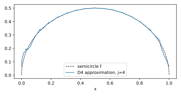
What is the set of all solutions to the dilation equation
\begin{equation*} \begin{aligned} \phi(x)={}&\frac{1+\sqrt3}{4}\phi(2x)+\frac{3+\sqrt3}{4}\phi(2x-1)\\ &+\frac{3-\sqrt3}{4}\phi(2x-2)+\frac{1-\sqrt3}{4}\phi(2x-3)\ ? \end{aligned} \end{equation*}
Among integrable functions, the solutions are exactly the scalar multiples \(\{\alpha\,\phi_{D_4}:\alpha\in\mathbb R\}\). Here \(\phi_{D_4}\) is the Daubechies scale function of Exercise 11.9: continuous, supported on \([0,3]\), \(\int\phi_{D_4}=1\), \(\phi_{D_4}(1)=\frac{1+\sqrt3}2\), \(\phi_{D_4}(2)=\frac{1-\sqrt3}2\). (The printed last coefficient \(\frac{1\sqrt3}{4}\) should be \(\frac{1-\sqrt3}{4}\).)
Existence: \(\phi_{D_4}\) is the limit of the cascade iteration of Section 11.4 (Daubechies’ theorem; computed in Exercise 11.9), so every multiple \(\alpha\phi_{D_4}\) solves the equation by linearity.
Uniqueness: let \(\phi\in L^1(\mathbb R)\) be any solution and put \(m(\omega)=\frac12\sum_{k=0}^3c_ke^{-ik\omega}\), so \(m(0)=\frac12\sum c_k=1\). Taking Fourier transforms, with \(\int\phi(2x-k)e^{-i\omega x}dx=\frac12e^{-ik\omega/2}\hat\phi(\omega/2)\),
\begin{equation*} \hat\phi(\omega)=m(\tfrac\omega2)\,\hat\phi(\tfrac\omega2)=\cdots =\Big(\prod_{n=1}^{N}m(\tfrac{\omega}{2^n})\Big)\hat\phi(\tfrac{\omega}{2^N}). \end{equation*}
Since \(|m(\omega)-1|\le\frac12\sum_k|c_k|\,k\,|\omega|=C|\omega|\), we get \(\sum_n|m(\omega/2^n)-1|\le C|\omega|\). So the product converges, uniformly on compact sets, to a continuous \(P(\omega)\) that does not depend on \(\phi\). Also \(\hat\phi\) is continuous (\(\phi\in L^1\)), so \(\hat\phi(\omega/2^N)\to\hat\phi(0)\). Letting \(N\to\infty\),
\begin{equation*} \hat\phi(\omega)=\hat\phi(0)\,P(\omega)\quad\text{for all }\omega, \qquad\text{in particular}\qquad \hat\phi_{D_4}=P . \end{equation*}
Hence \(\hat\phi=\hat\phi(0)\,\hat\phi_{D_4}\). Because the Fourier transform is injective on \(L^1\), \(\phi=\alpha\,\phi_{D_4}\) with \(\alpha=\hat\phi(0)=\int\phi\); the case \(\int\phi=0\) gives \(\phi=0\). \(\blacksquare\)
Prove that if scale functions defined by a dilation equation are orthogonal, then the sum of the even coefficients must equal the sum of the odd coefficients in the dilation equation. That is, \(\sum_k c_{2k}=\sum_k c_{2k+1}\).
Let \(E=\sum_kc_{2k}\) and \(O=\sum_kc_{2k+1}\); we show \(E+O=2\) and \(E^2+O^2=2\), which together force \(E=O=1\).
Setting: \(\phi(x)=\sum_{k=0}^{d-1}c_k\phi(2x-k)\), with \(\phi\) integrable, \(\int\phi\ne0\) (a scale function, Section 11.5), and orthogonal shifts normalized to \(\int\phi(x)\phi(x-k)\,dx=\delta(k)\). Lemma 11.1 applies (\(\|\phi\|_1<\infty\), \(\int\phi\ne0\)) and gives \(\sum_ic_i=E+O=2\). Lemma 11.2 applies (orthonormal shifts) and gives \(\sum_ic_ic_{i-2k}=2\delta(k)\) for every integer \(k\). Sum this over all \(k\); every sum is finite, since \(c_i=0\) outside \(0\le i\le d-1\). For each \(i\), \(\{i-2k:k\in\mathbb Z\}\) is the set of integers with the parity of \(i\), so
\begin{equation*} \begin{aligned} 2=\sum_k\sum_i c_ic_{i-2k}=\sum_i c_i\sum_k c_{i-2k} &=\sum_{i\text{ even}}c_i\,E+\sum_{i\text{ odd}}c_i\,O=E^2+O^2,\\ (E-O)^2=2(E^2+O^2)-(E+O)^2&=4-4=0 . \end{aligned} \end{equation*}
Hence \(\sum_kc_{2k}=\sum_kc_{2k+1}\;(=1)\). \(\blacksquare\)
Appendix
Exercises 12.1–12.7
What is the difference between saying \(f(n)\) is \(O(n^3)\) and \(f(n)\) is \(o(n^3)\)?
\(O(n^3)\) says \(f\) grows no faster than \(n^3\) up to a constant; \(o(n^3)\) says \(f\) grows strictly slower than \(n^3\). By Definition 12.1 and Section 12.2,
\begin{equation*} \begin{aligned} f(n)\text{ is }O(n^3) &\iff \exists\, c>0\ \forall n:\ f(n)\le c\,n^3,\\ f(n)\text{ is }o(n^3) &\iff \lim_{n\to\infty}\frac{f(n)}{n^3}=0 . \end{aligned} \end{equation*}
So \(O\) only requires the ratio \(f(n)/n^3\) to stay bounded, while \(o\) requires it to tend to \(0\). Little \(o\) is the stronger statement: a ratio tending to \(0\) is convergent, hence bounded by some \(c\), so \(f\) is \(O(n^3)\). The converse fails: \(f(n)=5n^3\) is \(O(n^3)\), but \(f(n)/n^3=5\not\to 0\). \(\blacksquare\)
If \(f(n)\sim g(n)\), what can we say about \(f(n)+g(n)\) and \(f(n)-g(n)\)?
\(f(n)+g(n)\sim 2g(n)\) (equivalently \(\sim 2f(n)\)), and \(f(n)-g(n)=o(g(n))\), i.e. the difference is of lower order than \(g\), but nothing more can be said about it. Since \(f(n)/g(n)\to 1\) (Section 12.2),
\begin{equation*} \begin{aligned} \frac{f(n)+g(n)}{2g(n)} &= \frac12\Big(\frac{f(n)}{g(n)}+1\Big)\ \longrightarrow\ 1,\\ \frac{f(n)-g(n)}{g(n)} &= \frac{f(n)}{g(n)}-1\ \longrightarrow\ 0 . \end{aligned} \end{equation*}
Since \(f-g\) need not be positive (it lies outside the positive-valued setting of Definition 12.1), the second statement means \(|f(n)-g(n)|/g(n)\to 0\). Beyond that, the sign and size of \(f-g\) are unconstrained, and it need not even be bounded: (i) \(f=g=n^2\) gives \(f-g=0\); (ii) \(f=n^2+n\), \(g=n^2\) gives \(f-g=n\); (iii) \(f=n^2\), \(g=n^2+n^{3/2}\) gives \(f-g=-n^{3/2}\). \(\blacksquare\)
What is the difference between \(\sim\) and \(\Theta\)?
\(f\sim g\) pins the ratio \(f/g\) down to the limit \(1\). \(f\) is \(\Theta(g)\) only traps the ratio between two positive constants. By Section 12.2,
\begin{equation*} \begin{aligned} f(n)\sim g(n) &\iff \lim_{n\to\infty}\frac{f(n)}{g(n)}=1,\\ f(n)\text{ is }\Theta(g(n)) &\iff \exists\, c_1,c_2>0\ \forall n:\ c_1\le \frac{f(n)}{g(n)}\le c_2 . \end{aligned} \end{equation*}
(i) \(\sim\) implies \(\Theta\). The ratio \(r_n=f(n)/g(n)\) converges, so it is bounded above. It also satisfies \(r_n\ge \tfrac12\) for all \(n\ge N\), and since \(f\) and \(g\) are positive, \(c_1=\min\{\tfrac12,r_1,\dots,r_{N-1}\}>0\). (ii) \(\Theta\) does not imply \(\sim\). The constant can differ from \(1\): \(f(n)=2n^2\) is \(\Theta(n^2)\), but \(f(n)/n^2=2\). The ratio also need not converge at all: \(f(n)=(2+(-1)^n)\,n\) is \(\Theta(n)\), since \(1\le f(n)/n\le 3\), but \(f(n)/n\) alternates between \(1\) and \(3\). \(\blacksquare\)
If \(f(n)\) is \(O(g(n))\), does this imply that \(g(n)\) is \(\Omega(f(n))\)?
Yes. By Definition 12.1 there is a \(c>0\) with \(f(n)\le c\,g(n)\) for all \(n\), so
\begin{equation*} g(n)\ \ge\ \frac1c\,f(n)\qquad\text{for all } n , \end{equation*}
and \(c^{\prime}=1/c>0\) witnesses that \(g(n)\) is \(\Omega(f(n))\) (Section 12.2). \(\blacksquare\)
What is \(\displaystyle\lim_{k\to\infty}\Big(\frac{k-1}{k-2}\Big)^{k-2}\)?
The limit is \(e\). Put \(m=k-2\to\infty\). Then \(\frac{k-1}{k-2}=1+\frac1m\), and
\begin{equation*} \lim_{k\to\infty}\Big(\frac{k-1}{k-2}\Big)^{k-2}=\lim_{m\to\infty}\Big(1+\frac1m\Big)^{m}=e , \end{equation*}
the last step because \(m\ln(1+\tfrac1m)=1-\tfrac1{2m}+O(m^{-2})\to 1\). \(\blacksquare\)
Select \(a\), \(b\), and \(c\) uniformly at random from \([0,1]\). The probability that \(b<a\) is \(1/2\). The probability that \(c<a\) is \(1/2\). However, the probability that both \(b\) and \(c\) are less than \(a\) is \(\frac13\), not \(1/4\). Why is this? Note that the six possible permutations \(abc\), \(acb\), \(bac\), \(cab\), \(bca\), and \(cba\) are all equally likely. Assume that \(a\), \(b\), and \(c\) are drawn from the interval \((0,1]\). Given that \(b<a\), what is the probability that \(c<a\)?
The events \(\{b<a\}\) and \(\{c<a\}\) are not independent, so their probabilities do not multiply. Given \(b<a\), the probability that \(c<a\) is \(2/3\).
The event that both hold is the event that \(a\) is the largest of the three. Ties have probability \(0\), and the six orderings are equally likely, so the event has probability \(2/6=1/3\). Conditionally on \(a\), the events are independent, each with probability \(a\), so
\begin{equation*} \begin{aligned} \text{Prob}(b<a,\ c<a) &= \int_0^1 a^2\,da=\frac13,\\ \text{Prob}(b<a)\,\text{Prob}(c<a) &= \Big(\int_0^1 a\,da\Big)^2=\frac14 , \end{aligned} \end{equation*}
and these differ because \(E(a^2)\ne (E\,a)^2\): learning \(b<a\) makes a large \(a\) more likely, which makes \(c<a\) more likely. Hence
\begin{equation*} \text{Prob}(c<a\mid b<a)=\frac{\text{Prob}(b<a,\ c<a)}{\text{Prob}(b<a)} =\frac{1/3}{1/2}=\frac23 . \qquad\blacksquare \end{equation*}
Let \(A_1,A_2,\dots,A_n\) be events. Prove that \(\displaystyle \text{Prob}(A_1\cup A_2\cup\cdots\cup A_n)\le \sum_{i=1}^n \text{Prob}(A_i)\).
Split the union into disjoint pieces. Let \(B_1=A_1\) and \(B_i=A_i\setminus(A_1\cup\cdots\cup A_{i-1})\) for \(i\ge 2\). The \(B_i\) are pairwise disjoint: if \(i<j\), then \(B_j\) avoids \(A_i\supseteq B_i\). Each \(B_i\subseteq A_i\). And \(\bigcup_{i}B_i=\bigcup_i A_i\), because a point of the union lies in \(B_i\) for the smallest \(i\) with that point in \(A_i\). Additivity on disjoint events and monotonicity then give
\begin{equation*} \begin{aligned} \text{Prob}\Big(\bigcup_{i=1}^n A_i\Big)=\text{Prob}\Big(\bigcup_{i=1}^n B_i\Big) &=\sum_{i=1}^n \text{Prob}(B_i)\\ &\le \sum_{i=1}^n \text{Prob}(A_i). \qquad\blacksquare \end{aligned} \end{equation*}
Method (2): Use induction on \(n\); the case \(n=1\) is equality. For two events, inclusion-exclusion (Boole’s formula, Section 12.5.3) gives \(\text{Prob}(A\cup B)=\text{Prob}(A)+\text{Prob}(B)-\text{Prob}(A\cap B)\le \text{Prob}(A)+\text{Prob}(B)\). Applying this with \(A=A_1\cup\cdots\cup A_{n-1}\) and \(B=A_n\), and then using the induction hypothesis on \(A\), gives the claim. \(\blacksquare\)
Exercises 12.8–12.14
Give an example of three random variables that are pairwise independent but not fully independent.
Let \(x,y\) be independent fair bits in \(\{0,1\}\) and \(z=x\oplus y=(x+y)\bmod 2\). Each of \(x,y,z\) is a fair bit, and for every pair, e.g. \((x,z)\), and all \(a,c\in\{0,1\}\),
\begin{equation*} \begin{aligned} \text{Prob}(x=a,\,z=c)&=\text{Prob}(x=a,\,y=a\oplus c)\\ &=\tfrac14=\text{Prob}(x=a)\,\text{Prob}(z=c), \end{aligned} \end{equation*}
and likewise for \((y,z)\), while \((x,y)\) is independent by construction; so the three are pairwise independent in the sense of Section 12.5.1. But \(z\) is determined by \(x,y\):
\begin{equation*} \begin{aligned} \text{Prob}(x=0,\,y=0,\,z=1)&=0\\ &\ne\tfrac18=\text{Prob}(x=0)\,\text{Prob}(y=0)\,\text{Prob}(z=1), \end{aligned} \end{equation*}
so they are not mutually independent.
Give examples of nonnegative valued random variables with median \(\gg\) mean. Can we have median \(\ll\) mean?
The first request cannot be met as printed: a nonnegative random variable always has median \(\le 2\cdot\)mean, while median \(\ll\) mean is easy. If \(M>0\) is a median of \(x\ge 0\) then \(\text{Prob}(x\ge M)\ge\frac12\), so Markov’s inequality (Theorem 2.1) gives
\begin{equation*} \tfrac12\le\text{Prob}(x\ge M)\le\frac{E(x)}{M}\quad\Longrightarrow\quad M\le 2E(x). \end{equation*}
The factor \(2\) is essentially attained: \(x=0\) with probability \(\frac12-\varepsilon\) and \(x=1\) with probability \(\frac12+\varepsilon\) has median \(1\) and mean \(\frac12+\varepsilon\).
Median \(\ll\) mean: yes. Let \(x=0\) with probability \(\frac23\) and \(x=N\) with probability \(\frac13\). Then
\begin{equation*} \text{median}(x)=0,\qquad E(x)=\frac N3\to\infty\quad(N\to\infty). \end{equation*}
Consider \(n\) samples \(x_1,x_2,\ldots,x_n\) from a Gaussian distribution of mean \(\mu\) and variance \(\sigma\). For this distribution \(m=\frac{x_1+x_2+\cdots+x_n}{n}\) is an unbiased estimator of \(\mu\). If \(\mu\) is known then \(\frac1n\sum_{i=1}^n(x_i-\mu)^2\) is an unbiased estimator of \(\sigma^2\). Prove that if we approximate \(\mu\) by \(m\), then \(\frac{1}{n-1}\sum_{i=1}^n(x_i-m)^2\) is an unbiased estimator of \(\sigma^2\).
The variance is meant to be \(\sigma^2\) (the book prints \(\sigma\)). Writing \(x_i-\mu=(x_i-m)+(m-\mu)\) and using \(\sum_i(x_i-m)=0\),
\begin{equation*} \sum_{i=1}^n(x_i-\mu)^2=\sum_{i=1}^n(x_i-m)^2+n(m-\mu)^2 . \end{equation*}
The samples are independent, so (Section 12.5.6, variance of a sum of independent variables) \(\text{Var}(m)=\frac{1}{n^2}\cdot n\sigma^2=\frac{\sigma^2}{n}\), i.e. \(E(m-\mu)^2=\sigma^2/n\). Taking expectations,
\begin{equation*} E\sum_{i=1}^n(x_i-m)^2=n\sigma^2-n\cdot\frac{\sigma^2}{n}=(n-1)\sigma^2, \end{equation*}
hence \(E\Big[\frac{1}{n-1}\sum_{i=1}^n(x_i-m)^2\Big]=\sigma^2\).
Given the distribution \(\frac{1}{\sqrt{2\pi}\,3}e^{-\frac12\left(\frac x3\right)^2}\), what is the probability that \(x>1\)?
\(\text{Prob}(x>1)=1-\Phi(1/3)\approx 0.3694\), where \(\Phi\) is the standard normal distribution function. Indeed the density is that of a Gaussian with mean \(0\) and standard deviation \(3\), so \(z=x/3\) is standard normal and
\begin{equation*} \text{Prob}(x>1)=\text{Prob}\Big(z>\tfrac13\Big) =\frac{1}{\sqrt{2\pi}}\int_{1/3}^{\infty}e^{-z^2/2}\,dz\approx 0.3694 . \end{equation*}
\(e^{-\frac{x^2}{2}}\) has value \(1\) at \(x=0\) and drops off very fast as \(x\) increases. Suppose we wished to approximate \(e^{-\frac{x^2}{2}}\) by a function \(f(x)\) where
\begin{equation*} f(x)=\begin{cases}1 & |x|\le a\\ 0 & |x|>a.\end{cases} \end{equation*}
What value of \(a\) should we use? What is the integral of the error between \(f(x)\) and \(e^{-\frac{x^2}{2}}\)?
Use \(a=\sqrt{2\ln 2}\approx 1.1774\), the point where \(e^{-x^2/2}=\frac12\); the integrated absolute error is then \(\approx 1.0465\). Write \(g(x)=e^{-x^2/2}\) and \(\Phi\) for the standard normal distribution function, so \(\int_{-a}^a g=\sqrt{2\pi}\,(2\Phi(a)-1)\) and \(\int_{|x|>a}g=2\sqrt{2\pi}\,(1-\Phi(a))\). Then
\begin{equation*} \begin{aligned} E(a)&=\int_{-\infty}^{\infty}|f-g|\,dx=\int_{-a}^{a}(1-g)\,dx+\int_{|x|>a}g\,dx\\ &=2a+\sqrt{2\pi}\,\big(3-4\Phi(a)\big),\\ E^{\prime}(a)&=2-4g(a)=0\iff e^{-a^2/2}=\tfrac12\iff a=\sqrt{2\ln 2}, \end{aligned} \end{equation*}
and \(E^{\prime\prime}(a)=4a\,g(a)>0\), so this is the minimum, with
\begin{equation*} \begin{aligned} E\big(\sqrt{2\ln2}\big)&=2\sqrt{2\ln 2}+\sqrt{2\pi}\,\big(3-4\Phi(1.1774)\big)\\ &\approx 2.3548-1.3083=1.0465 . \end{aligned} \end{equation*}
Method (2): if instead one asks that \(f\) have the same area as \(g\), then \(2a=\int g=\sqrt{2\pi}\), i.e. \(a=\sqrt{\pi/2}\approx1.2533\); the signed integral of the error \(\int(f-g)\,dx\) is then \(0\), and the integral of the absolute error is \(2a+\sqrt{2\pi}(3-4\Phi(a))\approx1.0532\), slightly worse than the optimum above.
Given two sets of red and black balls with the number of red and black balls in each set shown in the table below.
| red | black | |
|---|---|---|
| Set 1 | 40 | 60 |
| Set 2 | 50 | 50 |
Randomly draw a ball from one of the sets. Suppose that it turns out to be red. What is the probability that it was drawn from Set 1?
\(4/9\), taking the set to be chosen uniformly at random. By Bayes rule (Section 12.5.10), with \(\text{Prob}(\text{red}\mid 1)=\frac{40}{100}\) and \(\text{Prob}(\text{red}\mid 2)=\frac{50}{100}\),
\begin{equation*} \text{Prob}(1\mid\text{red}) =\frac{\frac12\cdot 0.4}{\frac12\cdot0.4+\frac12\cdot0.5}=\frac{0.2}{0.45}=\frac49 . \end{equation*}
Why cannot one prove an analogous type of theorem that states \(p(x\le a)\le\frac{E(x)}{a}\)?
Because it is false: take \(x\equiv 0\), which is nonnegative with \(E(x)=0\), yet \(p(x\le a)=1>0=E(x)/a\) for every \(a>0\). More generally \(p(x\le a)\to1\) as \(a\to\infty\) while \(E(x)/a\to0\) whenever \(E(x)<\infty\), so no such bound can hold for large \(a\). Markov’s inequality (Theorem 2.1) rests on \(x\ge a\,\mathbf 1\{x\ge a\}\) for \(x\ge0\): large values must contribute to the mean, whereas small values may contribute nothing, so the mean caps only the upper tail; Markov yields just the lower bound
\begin{equation*} p(x\le a)\ \ge\ 1-p(x\ge a)\ \ge\ 1-\frac{E(x)}{a}. \end{equation*}
Exercises 12.15–12.21
Compare the Markov and Chebyshev bounds for the following probability distributions:
(1) \(p(x) = \begin{cases} 1 & x = 1 \\ 0 & \text{otherwise} \end{cases}\)
(2) \(p(x) = \begin{cases} 1/2 & 0 \le x \le 2 \\ 0 & \text{otherwise} \end{cases}\)
Chebyshev is exact for the point mass and wins for the uniform law only in the far tail (\(t > (1+\sqrt{13})/6 \approx 0.768\)). Both distributions have \(m = E(x) = 1\), so with the bounds of Section 12.6.1 written as \(\Pr(x \ge a) \le E(x)/a\) and \(\Pr(|x-m| \ge t) \le \sigma^2/t^2\) (Chebyshev with \(t = a\sigma\)):
(1) Here \(\sigma^2 = 0\) and \(x \equiv 1\).
- Markov: \(\Pr(x \ge a) \le 1/a\). The truth is \(1\) for \(a \le 1\) and \(0\) for \(a > 1\), so Markov is tight only at \(a = 1\) and gives a nonzero bound \(1/a\) where the probability is \(0\).
- Chebyshev: \(\Pr(|x-1| \ge t) \le 0/t^2 = 0\) for every \(t > 0\), which is exact.
(2) Here \(\sigma^2 = \int_0^2 \tfrac12 (x-1)^2\,dx = 1/3\), and for \(0 \le t \le 1\)
\begin{equation*} \Pr(x \ge 1+t) = \frac{1-t}{2}, \qquad \Pr(|x-1| \ge t) = 1-t, \end{equation*}
while both probabilities are \(0\) for \(t > 1\). The bounds are
\begin{equation*} \Pr(x \ge 1+t) \le \frac{1}{1+t} \ \text{(Markov)}, \qquad \Pr(x \ge 1+t) \le \Pr(|x-1| \ge t) \le \frac{1}{3t^2} \ \text{(Chebyshev)}. \end{equation*}
Chebyshev is the smaller of the two exactly when \(3t^2 > 1+t\), i.e. \(t > (1+\sqrt{13})/6 \approx 0.768\); it is vacuous for \(t \le 1/\sqrt3 \approx 0.577\). Sample values:
| \(t\) | Markov \(1/(1+t)\) | Chebyshev \(1/(3t^2)\) | true \(\Pr(x \ge 1+t)\) | true \(\Pr(\lvert x-1 \rvert \ge t)\) |
|---|---|---|---|---|
| 0.25 | 0.800 | 5.333 (vacuous) | 0.375 | 0.75 |
| 0.50 | 0.667 | 1.333 (vacuous) | 0.250 | 0.50 |
| 0.75 | 0.571 | 0.593 | 0.125 | 0.25 |
| 0.90 | 0.526 | 0.412 | 0.050 | 0.10 |
| 1.00 | 0.500 | 0.333 | 0 | 0 |
Let \(s\) be the sum of \(n\) independent random variables \(x_1, x_2, \ldots, x_n\) where for each \(i\)
\begin{equation*} x_i = \begin{cases} 0 & \text{Prob } p \\ 1 & \text{Prob } 1-p. \end{cases} \end{equation*}
(1) How large must \(\delta\) be if we wish to have \(\mathrm{Prob}\big(s < (1-\delta)m\big) < \varepsilon\)?
(2) If we wish to have \(\mathrm{Prob}\big(s > (1+\delta)m\big) < \varepsilon\)?
With \(m = E(s) = n(1-p)\) and \(L = \ln(1/\varepsilon)\), it is enough to take \(\delta \ge \sqrt{2L/m}\) in part 1, and \(\delta \ge \sqrt{3L/m}\) in part 2 when that number is at most \(1\). Note that here \(x_i = 1\) with probability \(1-p\), so Theorems 12.3 and 12.4 apply with \(1-p\) in place of \(p\), still with \(m = E(s)\).
(1) By Theorem 12.4 (valid for \(0 < \delta \le 1\)),
\begin{equation*} \mathrm{Prob}\big(s < (1-\delta)m\big) < e^{-\delta^2 m/2} \le \varepsilon \iff \delta \ge \sqrt{\frac{2\ln(1/\varepsilon)}{n(1-p)}} . \end{equation*}
If this square root exceeds \(1\), take \(\delta = 1\): then \(\mathrm{Prob}(s < 0) = 0 < \varepsilon\). So \(\delta = \min\big\{1, \sqrt{2L/m}\big\}\) always suffices.
(2) By Theorem 12.3, \(\mathrm{Prob}\big(s > (1+\delta)m\big) < \big[e^{\delta}/(1+\delta)^{1+\delta}\big]^m\). The base is decreasing in \(\delta\), because its logarithm has derivative \(-\ln(1+\delta) < 0\). The exact requirement is therefore
\begin{equation*} (1+\delta)\ln(1+\delta) - \delta \ge \frac{\ln(1/\varepsilon)}{m}, \end{equation*}
which has a unique threshold \(\delta^\ast\). Two closed forms follow from it.
- (i) Small deviations (\(\delta \le 1\)). Put \(f(\delta) = \delta - (1+\delta)\ln(1+\delta) + \delta^2/3\). Then \(f(0) = f^{\prime}(0) = 0\) and \(f^{\prime\prime}(\delta) = \tfrac23 - \tfrac{1}{1+\delta}\), so \(f^{\prime}\) decreases on \([0,\tfrac12]\) and increases on \([\tfrac12,1]\), with \(f^{\prime}(1) = \tfrac23 - \ln 2 < 0\). Hence \(f^{\prime} \le 0\) and \(f \le 0\) on \([0,1]\). This gives
\begin{equation*} \mathrm{Prob}\big(s > (1+\delta)m\big) < e^{-\delta^2 m/3} \le \varepsilon \iff \delta \ge \sqrt{\frac{3\ln(1/\varepsilon)}{n(1-p)}}, \end{equation*}
which is usable whenever this root is at most \(1\).
- (ii) Large deviations (\(\delta > 2e-1\)). By the bound \(2^{-(1+\delta)m}\) derived after Theorem 12.3,
\begin{equation*} 2^{-(1+\delta)m} \le \varepsilon \iff \delta \ge \frac{\log_2(1/\varepsilon)}{n(1-p)} - 1, \end{equation*}
so \(\delta = \max\big\{2e-1,\ \log_2(1/\varepsilon)/m - 1\big\}\) always suffices.
What is the expected number of flips of a coin until a head is reached? Assume \(p\) is the probability of a head on an individual flip. What is the value if \(p = 1/2\)?
The expected number is \(1/p\), so \(2\) flips when \(p = 1/2\). Let \(N\) be the number of flips up to and including the first head. Then \(\Pr(N = k) = (1-p)^{k-1}p\), so
\begin{equation*} E(N) = \sum_{k \ge 1} k(1-p)^{k-1} p = \frac{p}{\big(1-(1-p)\big)^2} = \frac1p , \end{equation*}
using \(\sum_{k\ge1} k q^{k-1} = 1/(1-q)^2\) for \(|q| < 1\). When \(p = 1/2\), \(E(N) = 2\).
Given the joint probability
| \(P(A,B)\) | \(A=0\) | \(A=1\) |
|---|---|---|
| \(B=0\) | \(1/16\) | \(1/8\) |
| \(B=1\) | \(1/4\) | \(9/16\) |
(1) What is the marginal probability of \(A\)? Of \(B\)?
(2) What is the conditional probability of \(B\) given \(A\)?
(1) The marginals are \(P(A=0) = 5/16\), \(P(A=1) = 11/16\) and \(P(B=0) = 3/16\), \(P(B=1) = 13/16\). They come from summing the columns and the rows of the table:
\begin{equation*} \begin{aligned} P(A=0) &= \tfrac1{16} + \tfrac14 = \tfrac5{16}, & P(A=1) &= \tfrac18 + \tfrac9{16} = \tfrac{11}{16},\\ P(B=0) &= \tfrac1{16} + \tfrac18 = \tfrac3{16}, & P(B=1) &= \tfrac14 + \tfrac9{16} = \tfrac{13}{16}. \end{aligned} \end{equation*}
(2) Using \(P(B \mid A) = P(A,B)/P(A)\):
\begin{equation*} \begin{aligned} P(B=0 \mid A=0) &= \tfrac{1/16}{5/16} = \tfrac15, & P(B=1 \mid A=0) &= \tfrac{4/16}{5/16} = \tfrac45,\\ P(B=0 \mid A=1) &= \tfrac{2/16}{11/16} = \tfrac2{11}, & P(B=1 \mid A=1) &= \tfrac{9/16}{11/16} = \tfrac9{11}. \end{aligned} \end{equation*}
Consider independent random variables \(x_1\), \(x_2\), and \(x_3\), each equal to zero with probability \(\frac12\). Let \(S = x_1 + x_2 + x_3\) and let \(F\) be the event that \(S \in \{1, 2\}\). Conditioning on \(F\), the variables \(x_1\), \(x_2\), and \(x_3\) are still each zero with probability \(\frac12\). Are they still independent?
No, not even pairwise. Each \(x_i\) is \(0\) or \(1\) with probability \(\frac12\), so all \(8\) outcomes are equally likely. \(F\) removes \(000\) and \(111\), which leaves \(6\) equally likely outcomes. Each \(x_i\) is zero in exactly \(3\) of them, which gives the stated \(\Pr(x_i = 0 \mid F) = \frac12\). However, \(x_1 = x_2 = 0\) holds only for the outcome \(001\), so
\begin{equation*} \Pr(x_1 = 0, x_2 = 0 \mid F) = \frac16 \ne \frac14 = \Pr(x_1 = 0 \mid F)\Pr(x_2 = 0 \mid F). \end{equation*}
Consider rolling two dice \(A\) and \(B\). What is the probability that the sum \(S\) will add to nine? What is the probability that the sum will be \(9\) if the roll of \(A\) is \(3\)?
The answers are \(\Pr(S = 9) = 1/9\) and \(\Pr(S = 9 \mid A = 3) = 1/6\). Of the \(36\) equally likely pairs, the four pairs \((3,6), (4,5), (5,4), (6,3)\) sum to \(9\), so \(\Pr(S=9) = 4/36 = 1/9\). Given \(A = 3\), the sum is \(9\) exactly when \(B = 6\). Since \(B\) is independent of \(A\), \(\Pr(S = 9 \mid A = 3) = \Pr(B = 6) = 1/6\).
Write the generating function for the number of ways of producing change using only pennies, nickels, and dimes. In how many ways can you produce \(23\) cents?
The generating function is
\begin{equation*} g(x) = \frac{1}{(1-x)(1-x^5)(1-x^{10})}, \end{equation*}
and there are \(9\) ways to make \(23\) cents. The book prints “chains” and “dines” for “change” and “dimes”. As in Section 12.9, where selections are multiplied together, \(g(x)\) is the product of \(1 + x^{c} + x^{2c} + \cdots = 1/(1-x^c)\) over the three coins \(c = 1, 5, 10\). The coefficient of \(x^n\) is the number of \((a, b, d) \ge 0\) with \(a + 5b + 10d = n\).
For \(n = 23\), sort by the number of dimes \(d\). The pennies are then forced, and the nickels \(b\) range over \(0, \ldots, \lfloor (23-10d)/5 \rfloor\):
\begin{equation*} [x^{23}]\,g(x) = \underbrace{5}_{d=0} + \underbrace{3}_{d=1} + \underbrace{1}_{d=2} = 9 . \end{equation*}
Exercises 12.22–12.28
A die has six faces, each face having one of the numbers 1 through 6. The result of a roll of the die is the integer on the top face. Consider two rolls of the die. In how many ways can an integer be the sum of two rolls of the die?
The sum \(s\) arises in \(6-|s-7|\) ordered ways for \(2\le s\le 12\) (and in no way otherwise). A single roll has generating function \(x+x^2+\cdots+x^6\), and by the product rule for independent selections in Section 12.9 the number of ordered pairs of rolls with sum \(s\) is the coefficient of \(x^s\) in
\begin{equation*} \begin{aligned} (x+x^2+\cdots+x^6)^2 &= x^2\Big(\frac{1-x^6}{1-x}\Big)^2\\ &= x^2+2x^3+3x^4+4x^5+5x^6+6x^7\\ &\quad +5x^8+4x^9+3x^{10}+2x^{11}+x^{12}. \end{aligned} \end{equation*}
| sum \(s\) | 2 | 3 | 4 | 5 | 6 | 7 | 8 | 9 | 10 | 11 | 12 |
|---|---|---|---|---|---|---|---|---|---|---|---|
| ways | 1 | 2 | 3 | 4 | 5 | 6 | 5 | 4 | 3 | 2 | 1 |
If \(a(x)\) is the generating function for the sequence \(a_0,a_1,a_2,\ldots\), for what sequence is \(a(x)(1-x)\) the generating function?
It generates the sequence of differences \(a_0,\ a_1-a_0,\ a_2-a_1,\ a_3-a_2,\ldots\):
\begin{equation*} \begin{aligned} (1-x)\sum_{i\ge 0}a_ix^i &= \sum_{i\ge 0}a_ix^i-\sum_{i\ge 1}a_{i-1}x^i\\ &= a_0+\sum_{i\ge 1}(a_i-a_{i-1})x^i . \end{aligned} \end{equation*}
How many ways can one draw \(n\) \(a\)’s and \(b\)’s with an even number of \(a\)’s?
\(2^{n-1}\) ways for \(n\ge 1\) (and \(1\) way for \(n=0\)) if the draws are ordered; \(\lfloor n/2\rfloor+1\) ways if only the numbers of \(a\)’s and \(b\)’s matter. The statement does not say which, so both readings are treated.
(i) Ordered draws (words of length \(n\)). Choosing which \(k\) positions hold \(a\)’s, the count is the sum of the even-index coefficients of \((1+y)^n\):
\begin{equation*} \begin{aligned} \sum_{k\ \text{even}}\binom nk &= \frac{(1+1)^n+(1-1)^n}{2}\\ &= \begin{cases} 2^{n-1}, & n\ge 1,\\ 1, & n=0.\end{cases} \end{aligned} \end{equation*}
(ii) Unordered draws (selections, as in the \(A\), \(B\), \(C\) example of Section 12.9). The \(a\)’s contribute \(1+x^2+x^4+\cdots\) and the \(b\)’s \(1+x+x^2+\cdots\), so the count is the coefficient of \(x^n\) in
\begin{equation*} \frac{1}{(1-x^2)(1-x)}=\sum_{n\ge 0}\Big(\Big\lfloor\frac n2\Big\rfloor+1\Big)x^n , \end{equation*}
since each even \(2j\le n\) of \(a\)’s, \(j=0,\ldots,\lfloor n/2\rfloor\), leaves exactly one way to complete with \(b\)’s.
Find the generating function for the recurrence \(a_i=2a_{i-1}+i\) where \(a_0=1\).
\begin{equation*} a(x)=\frac{1-x+x^2}{(1-x)^2(1-2x)}=\frac{3}{1-2x}-\frac{1}{1-x}-\frac{1}{(1-x)^2}, \end{equation*}
so \(a_n=3\cdot 2^n-n-2\). As in Section 12.9.1, multiply the recurrence by \(x^i\) and sum over \(i\ge 1\), using \(\sum_{i\ge 1}ix^i=x/(1-x)^2\) (the example in Section 12.9):
\begin{equation*} \begin{aligned} a(x)-a_0 &= 2x\,a(x)+\frac{x}{(1-x)^2},\\ (1-2x)\,a(x) &= 1+\frac{x}{(1-x)^2}=\frac{1-x+x^2}{(1-x)^2}. \end{aligned} \end{equation*}
Partial fractions give the second form (Check!), and expanding \(\frac{1}{1-2x}=\sum 2^nx^n\), \(\frac1{1-x}=\sum x^n\), \(\frac1{(1-x)^2}=\sum (n+1)x^n\) yields
\begin{equation*} a_n=3\cdot 2^n-1-(n+1)=3\cdot 2^n-n-2, \end{equation*}
giving \(1,3,8,19,42,89,\ldots\)
Find a closed form for the generating function for the infinite sequence of perfect squares \(1,4,9,16,25,\ldots\)
\begin{equation*} \sum_{n\ge 0}(n+1)^2x^n=\frac{1+x}{(1-x)^3}. \end{equation*}
By Section 12.9, if \(g(x)=\frac1{1-x}\) generates \(1,1,1,\ldots\) then \(x^2g^{\prime\prime}(x)+xg^{\prime}(x)\) generates \(0,1,4,9,\ldots\), i.e. \(\sum_{n\ge0}n^2x^n\):
\begin{equation*} \begin{aligned} x^2g^{\prime\prime}+xg^{\prime} &= \frac{2x^2}{(1-x)^3}+\frac{x}{(1-x)^2}\\ &= \frac{2x^2+x(1-x)}{(1-x)^3}=\frac{x(1+x)}{(1-x)^3}. \end{aligned} \end{equation*}
Dropping the leading \(0\) (dividing by \(x\)) gives the generating function of \(1,4,9,16,\ldots\) indexed from \(a_0=1\); if the sequence is indexed as \(a_n=n^2\) with \(a_0=0\), the answer is \(x(1+x)/(1-x)^3\).
Given that \(\frac{1}{1-x}\) is the generating function for the sequence \(1,1,\ldots\), for what sequence is \(\frac{1}{1-2x}\) the generating function?
For \(1,2,4,8,\ldots\), i.e. \(a_i=2^i\): substituting \(2x\) for \(x\) in \(\frac1{1-x}=\sum_{i\ge0}x^i\) gives
\begin{equation*} \frac{1}{1-2x}=\sum_{i\ge 0}(2x)^i=\sum_{i\ge 0}2^ix^i . \end{equation*}
Find a closed form for the exponential generating function for the infinite sequence of perfect squares \(1,4,9,16,25,\ldots\)
\begin{equation*} \sum_{n\ge 0}(n+1)^2\frac{x^n}{n!}=(1+3x+x^2)\,e^x . \end{equation*}
With the exponential generating function of Section 12.9.2, \(e^x\) generates \(1,1,1,\ldots\), and \(x\frac{d}{dx}\) multiplies the \(n\)th term by \(n\), so \(\big(x\frac{d}{dx}\big)^2e^x=x(e^x+xe^x)=(x+x^2)e^x\) generates \(n^2\). Differentiating an exponential generating function shifts the sequence, \(\frac{d}{dx}\sum b_n\frac{x^n}{n!}=\sum b_{n+1}\frac{x^n}{n!}\), hence
\begin{equation*} \begin{aligned} \sum_{n\ge0}(n+1)^2\frac{x^n}{n!} &= \frac{d}{dx}\big[(x+x^2)e^x\big]\\ &= (1+2x)e^x+(x+x^2)e^x=(1+3x+x^2)e^x . \end{aligned} \end{equation*}
If the sequence is indexed as \(a_n=n^2\) with \(a_0=0\), the answer is \((x+x^2)e^x\).
Exercises 12.29–12.35
Prove that the \(L_2\) norm of \((a_1,a_2,\dots,a_n)\) is less than or equal to the \(L_1\) norm of \((a_1,a_2,\dots,a_n)\).
Square both sides: the square of the \(L_1\) norm contains the square of the \(L_2\) norm plus nonnegative cross terms,
\begin{equation*} \begin{aligned} |a|_1^2 = \Big(\sum_{i=1}^n |a_i|\Big)^2 &= \sum_{i=1}^n |a_i|^2 + \sum_{i\ne j} |a_i|\,|a_j| \\ &\ge \sum_{i=1}^n a_i^2 = |a|_2^2 . \end{aligned} \end{equation*}
Both norms are nonnegative, so taking square roots gives \(|a|_2 \le |a|_1\) (the case \(p=1\), \(q=2\) of Lemma 12.15). \(\blacksquare\)
Prove that there exists a \(y\), \(0 \le y \le x\), such that \(f(x) = f(0) + f^{\prime}(y)\,x\).
(Here \(x \ge 0\) and \(f\) is continuous on \([0,x]\) and differentiable on \((0,x)\), the hypotheses of the mean value theorem in Section 12.10.3.)
This is the mean value theorem on \([0,x]\); it follows from Rolle’s theorem applied to \(f\) minus its chord. If \(x=0\), take \(y=0\). If \(x>0\), put
\begin{equation*} g(t) = f(t) - f(0) - \frac{f(x)-f(0)}{x}\,t, \qquad 0 \le t \le x . \end{equation*}
Then \(g\) is continuous on \([0,x]\), differentiable on \((0,x)\), and \(g(0) = 0 = g(x)\) (Check!). By Rolle’s theorem there is \(y\in(0,x)\) with
\begin{equation*} 0 = g^{\prime}(y) = f^{\prime}(y) - \frac{f(x)-f(0)}{x} \quad\Longrightarrow\quad f(x) = f(0) + f^{\prime}(y)\,x . \qquad \blacksquare \end{equation*}
Show that the eigenvectors of a matrix \(A\) are not a continuous function of changes to the matrix.
Take the symmetric family
\begin{equation*} A(\varepsilon) = \begin{pmatrix} 1+\varepsilon & 0 \\ 0 & 1-\varepsilon \end{pmatrix}, \qquad \varepsilon\in\mathbb{R}, \end{equation*}
which depends continuously on \(\varepsilon\), as do its eigenvalues \(1\pm\varepsilon\). Let \(v(\varepsilon)\) be any unit eigenvector for the largest eigenvalue \(\lambda_1(A(\varepsilon))\). Then
\begin{equation*} v(\varepsilon) \in \begin{cases} \{\pm e_1\}, & \varepsilon > 0,\\ \{\pm e_2\}, & \varepsilon < 0, \end{cases} \end{equation*}
since for \(\varepsilon\ne 0\) the eigenvalues are distinct and each eigenspace is a coordinate axis. Every vector of \(\{\pm e_1\}\) is at distance \(\sqrt 2\) from every vector of \(\{\pm e_2\}\), so for all \(\varepsilon>0\)
\begin{equation*} |v(\varepsilon) - v(-\varepsilon)| = \sqrt 2 , \end{equation*}
while \(|A(\varepsilon)-A(-\varepsilon)|_F = 2\sqrt2\,\varepsilon \to 0\). Hence no choice of \(v(0)\) (and no choice of signs) makes \(\varepsilon\mapsto v(\varepsilon)\) continuous at \(\varepsilon=0\): an arbitrarily small perturbation of \(A(0)=I\) rotates the top eigenvector by \(90^\circ\). \(\blacksquare\)
What are the eigenvalues of the two graphs shown below? What does this say about using eigenvalues to determine if two graphs are isomorphic.
The figure shows (left) the 4-cycle \(C_4\): a square on 4 vertices with its 4 sides as edges; and (right) the star \(K_{1,4}\): one center vertex joined to each of 4 leaves, 5 vertices and 4 edges.
Both graphs have nonzero eigenvalues exactly \(2\) and \(-2\); the rest are \(0\):
\begin{equation*} \operatorname{spec}(C_4) = \{2,\,0,\,0,\,-2\}, \qquad \operatorname{spec}(K_{1,4}) = \{2,\,0,\,0,\,0,\,-2\}. \end{equation*}
For \(C_4\) with vertices \(1,2,3,4\) in cyclic order, a basis of eigenvectors is
\begin{equation*} A(1,1,1,1)^T = 2(1,1,1,1)^T,\quad A(1,-1,1,-1)^T = -2(1,-1,1,-1)^T, \end{equation*}
\begin{equation*} A(1,0,-1,0)^T = 0, \qquad A(0,1,0,-1)^T = 0 . \end{equation*}
For \(K_{1,4}\), list the center first: then \(A(\pm2,1,1,1,1)^T = \pm2(\pm2,1,1,1,1)^T\) (the center receives \(4\), each leaf receives \(\pm2\)), and each of the 3 independent vectors \((0,u)\) with \(u\in\mathbb{R}^4\), \(\sum_i u_i=0\), is sent to \(0\). Equivalently the characteristic polynomials are \(\lambda^2(\lambda^2-4)\) and \(\lambda^3(\lambda^2-4)\).
Adding one isolated vertex to \(C_4\) appends one eigenvalue \(0\), so \(C_4\cup K_1\) and \(K_{1,4}\) have the identical spectrum \(\{2,0,0,0,-2\}\), yet they are not isomorphic (\(K_{1,4}\) is connected and has a vertex of degree 4; \(C_4\cup K_1\) is disconnected and its maximum degree is 2).
Conclusion: isomorphic graphs always have the same eigenvalues, because relabelling vertices replaces \(A\) by \(P^TAP=P^{-1}AP\) for a permutation matrix \(P\) (Theorem 12.8), so differing spectra prove non-isomorphism. The converse fails: equal spectra do not imply isomorphism, so eigenvalues alone cannot decide whether two graphs are isomorphic.
Let \(A\) be the adjacency matrix of an undirected graph \(G\). Prove that eigenvalue \(\lambda_1\) of \(A\) is at least the average degree of \(G\).
Test the Rayleigh quotient on the all-ones vector. Since \(G\) is undirected, \(A\) is real symmetric, so by Theorem 12.12 with \(s=0\) (Section 12.8.3) \(\lambda_1 = \max_{|x|=1} x^TAx\). With \(n\) vertices, \(m\) edges and \(x = \frac{1}{\sqrt n}\mathbf 1\),
\begin{equation*} \lambda_1 \ge \frac{\mathbf 1^T A \mathbf 1}{n} = \frac{1}{n}\sum_{i,j} a_{ij} = \frac{1}{n}\sum_{i=1}^n d_i = \frac{2m}{n}, \end{equation*}
because the \(i\)-th row sum of \(A\) is the degree \(d_i\). The right side is the average degree. \(\blacksquare\)
Show that if \(A\) is a symmetric matrix and \(\lambda_1\) and \(\lambda_2\) are distinct eigenvalues then their corresponding eigenvectors \(x_1\) and \(x_2\) are orthogonal.
Hint: (left blank in the book).
Evaluate \(x_1^TAx_2\) in two ways, using \(A^T=A\):
\begin{equation*} \begin{aligned} \lambda_1\, x_1^Tx_2 = (Ax_1)^Tx_2 = x_1^TA^Tx_2 = x_1^TAx_2 = \lambda_2\, x_1^Tx_2 . \end{aligned} \end{equation*}
Hence \((\lambda_1-\lambda_2)\,x_1^Tx_2 = 0\), and since \(\lambda_1\ne\lambda_2\), \(x_1^Tx_2=0\). (The eigenvalues and eigenvectors may be taken real by Theorem 12.10.) \(\blacksquare\)
Show that a matrix is rank \(k\) if and only if it has \(k\) nonzero eigenvalues and eigenvalue \(0\) of rank \(n-k\).
As printed the claim fails for general square matrices (\(N=\begin{pmatrix}0&1\\0&0\end{pmatrix}\) has rank 1 but no nonzero eigenvalue), so we prove it for a diagonalizable \(n\times n\) matrix \(A\), in particular every real symmetric matrix (Theorem 12.10), reading “rank \(n-k\)” as multiplicity \(n-k\).
By Theorem 12.9, \(A = PDP^{-1}\) with \(P\) invertible and \(D=\operatorname{diag}(\lambda_1,\dots,\lambda_n)\). The \(\lambda_i\), counted with multiplicity, are the eigenvalues of \(A\), since \(\det(A-\lambda I) = \det(D-\lambda I) = \prod_i(\lambda_i-\lambda)\). Multiplying by invertible matrices does not change rank, so
\begin{equation*} \begin{aligned} \operatorname{rank} A = \operatorname{rank} D &= \#\{i : \lambda_i \ne 0\},\\ \dim\ker A = \dim\big(P\ker D\big) &= \#\{i : \lambda_i = 0\} = n - \operatorname{rank} A . \end{aligned} \end{equation*}
Thus \(\operatorname{rank}A = k\) holds exactly when \(A\) has \(k\) nonzero eigenvalues (with multiplicity), and this holds exactly when the eigenvalue \(0\) has algebraic multiplicity \(n-k\). That multiplicity also equals the dimension of the eigenspace \(\ker A\). \(\blacksquare\)
Exercises 12.36–12.42
Prove that maximizing \(\dfrac{x^TAx}{x^Tx}\) is equivalent to maximizing \(x^TAx\) subject to the condition that \(x\) be of unit length.
The quotient is invariant under scaling, so both problems range over the same set of values. For every \(x\ne 0\) and every scalar \(c\ne 0\),
\begin{equation*} \frac{(cx)^TA(cx)}{(cx)^T(cx)}=\frac{c^2\,x^TAx}{c^2\,x^Tx}=\frac{x^TAx}{x^Tx}. \end{equation*}
Taking \(c=1/|x|\) gives \(\frac{x^TAx}{x^Tx}=u^TAu\) with \(u=x/|x|\) a unit vector; conversely a unit \(u\) has \(\frac{u^TAu}{u^Tu}=u^TAu\). Hence
\begin{equation*} \Big\{\tfrac{x^TAx}{x^Tx}: x\ne 0\Big\}=\big\{u^TAu: |u|=1\big\}, \end{equation*}
so the two maxima are equal, and \(x\ne 0\) maximizes the quotient if and only if \(x/|x|\) maximizes \(u^TAu\) on the unit sphere (the maximizers of the quotient are exactly the nonzero multiples of the constrained maximizers). The unit sphere is compact, so the maximum exists.
Let \(A\) be a symmetric matrix with smallest eigenvalue \(\lambda_{\min}\). Give a bound on the largest element of \(A^{-1}\).
Every entry satisfies \(|(A^{-1})_{ij}|\le 1/|\lambda_{\min}|\), where \(\lambda_{\min}\) is the eigenvalue of smallest absolute value (the book’s smallest eigenvalue when \(A\) is positive definite; for indefinite \(A\) the algebraically smallest one gives no bound, as \(A=\mathrm{diag}(-1,\varepsilon)\) shows). Here \(A\) is invertible, so \(\lambda_{\min}\ne 0\). \(A^{-1}\) is symmetric with eigenvalues \(1/\lambda_1,\ldots,1/\lambda_n\) (if \(Av=\lambda v\) then \(A^{-1}v=\lambda^{-1}v\)), so Lemma 12.21 gives \(\|A^{-1}\|_2=\max_k 1/|\lambda_k|=1/|\lambda_{\min}|\). Then, by Cauchy-Schwarz and Lemma 12.24,
\begin{equation*} |(A^{-1})_{ij}|=|e_i^TA^{-1}e_j|\le |e_i|\,|A^{-1}e_j|\le \|A^{-1}\|_2=\frac{1}{|\lambda_{\min}|}. \end{equation*}
Let \(A\) be the adjacency matrix of an \(n\) vertex clique with no self loops. Thus, each row of \(A\) is all ones except for the diagonal entry which is zero. What is the spectrum of \(A\)?
The spectrum is \(n-1\) with multiplicity \(1\) and \(-1\) with multiplicity \(n-1\). Write \(A=J-I\) with \(J=\mathbf{1}\mathbf{1}^T\) the all-ones matrix. Then
\begin{equation*} \begin{aligned} A\mathbf{1}&=\mathbf{1}(\mathbf{1}^T\mathbf{1})-\mathbf{1}=(n-1)\mathbf{1},\\ Av&=\mathbf{1}(\mathbf{1}^Tv)-v=-v\qquad\text{for every } v\perp\mathbf{1}. \end{aligned} \end{equation*}
The vector \(\mathbf{1}\) and an orthonormal basis of the \((n-1)\)-dimensional space \(\mathbf{1}^\perp\) form a basis of eigenvectors, so these are all the eigenvalues, with the stated multiplicities.
Let \(A\) be the adjacency matrix of an undirected graph \(G\). Prove that the eigenvalue \(\lambda_1\) of \(A\) is at least the average degree of \(G\).
Test the Rayleigh quotient on \(x=\mathbf{1}/\sqrt n\). \(G\) is undirected, so \(A\) is real symmetric and Theorem 12.12 (with \(s=0\)) gives \(\lambda_1=\max_{|x|=1}x^TAx\). With \(d_i=\sum_j a_{ij}\) the degree of vertex \(i\),
\begin{equation*} \lambda_1\ \ge\ \frac{\mathbf{1}^TA\mathbf{1}}{n}=\frac1n\sum_{i=1}^n\sum_{j=1}^n a_{ij}=\frac1n\sum_{i=1}^n d_i , \end{equation*}
which is the average degree.
We are given the probability distribution for two random vectors \(x\) and \(y\) and we wish to stretch space to maximize the expected distance between them. Thus, we will multiply each coordinate by some quantity \(a_i\). We restrict \(\sum_{i=1}^d a_i^2=d\). Thus, if we increase some coordinate by \(a_i>1\), some other coordinate must shrink. Given random vectors \(x=(x_1,x_2,\ldots,x_d)\) and \(y=(y_1,y_2,\ldots,y_d)\), how should we select \(a_i\) to maximize \(E\big(|x-y|^2\big)\)? The \(a_i\) stretch different coordinates.
Assume
\begin{equation*} y_i=\begin{cases}0 & \text{with probability } \tfrac12\\ 1 & \text{with probability } \tfrac12\end{cases} \end{equation*}
and that \(x_i\) has some arbitrary distribution (the printed computation uses \(E(x_i^2)=E(x_i)\), i.e. \(x_i\in\{0,1\}\)). Why does weighting the coordinates have no effect? What if instead \(y_i=0\) with probability \(\frac34\) and \(y_i=1\) with probability \(\frac14\)? What if we used the 1-norm instead of the 2-norm? (The printed exercise sketches these computations.)
Put all the weight on a coordinate with the largest \(c_i=E\big((x_i-y_i)^2\big)\): \(a_{i^*}=\sqrt d\) for one \(i^*\in\arg\max_i c_i\) and \(a_i=0\) otherwise. With \(w_i=a_i^2\ge 0\), \(\sum_i w_i=d\),
\begin{equation*} E\big(|x-y|^2\big)=E\sum_{i=1}^d a_i^2(x_i-y_i)^2=\sum_{i=1}^d w_i c_i\ \le\ d\max_i c_i , \end{equation*}
by linearity of expectation (Section 12.5.2), with equality for that choice; any split of the weight among coordinates attaining \(\max_i c_i\) is equally good.
For the special cases take \(x_i\in\{0,1\}\) with \(p_i=\mathrm{Prob}(x_i=1)\), \(y_i\in\{0,1\}\) with \(\mathrm{Prob}(y_i=1)=q\), and \(y_i\) independent of \(x_i\) (needed for \(E(x_iy_i)=E(x_i)E(y_i)\)). Since \(x_i^2=x_i\) and \(y_i^2=y_i\),
\begin{equation*} c_i=E(x_i)-2E(x_i)E(y_i)+E(y_i)=p_i(1-2q)+q . \end{equation*}
(i) \(q=\frac12\): \(c_i=\frac12\) for every \(i\), whatever \(p_i\), so \(E(|x-y|^2)=\frac12\sum_i a_i^2=\frac d2\) for every admissible \(a\). Weighting has no effect because \(1-2q=0\): a fair coin \(y_i\) disagrees with \(x_i\) with probability \(\frac12\) regardless of the distribution of \(x_i\). (The printed text says “assuming \(\sum a_i^2=1\)”; under the stated constraint the constant is \(d/2\).)
(ii) \(q=\frac14\): \(c_i=\frac12p_i+\frac14\), so put all the weight (\(a_{i^*}=\sqrt d\)) on the coordinate with the largest \(p_i=\mathrm{Prob}(x_i=1)\), giving \(E(|x-y|^2)=d\big(\frac12\max_ip_i+\frac14\big)\).
(iii) 1-norm, with stretch factors \(a_i\ge 0\): setting \(b_i=E|x_i-y_i|\) (the printed \(b_i=E(x_i-y_i)\) is missing the absolute value), Cauchy-Schwarz gives
\begin{equation*} E\big(|x-y|_1\big)=\sum_{i=1}^d a_iE|x_i-y_i|=\sum_{i=1}^d a_ib_i\le |a|\,|b|=\sqrt d\,|b| , \end{equation*}
with equality if and only if \(a\) is parallel to \(b\), i.e. \(a_i=\sqrt d\,b_i/|b|\). For the 0/1 cases \(b_i=c_i\): in (i) all \(b_i=\frac12\), so \(a_i=1\) is optimal, and in (ii) \(a_i\propto \frac12p_i+\frac14\).
Maximize \(x+y\) subject to the constraint that \(x^2+y^2=1\).
The maximum is \(\sqrt2\), attained at \(x=y=\frac{1}{\sqrt2}\). With a Lagrange multiplier (Section 12.10.1), set the gradient of \(x+y+\lambda(x^2+y^2-1)\) to zero:
\begin{equation*} \begin{aligned} 1+2\lambda x&=0,\qquad 1+2\lambda y=0,\qquad x^2+y^2=1\\ &\Rightarrow\ x=y=-\tfrac{1}{2\lambda},\quad 2x^2=1\ \Rightarrow\ x=y=\pm\tfrac{1}{\sqrt2}. \end{aligned} \end{equation*}
The constraint set is a compact circle, so the continuous \(x+y\) attains its maximum at one of these two critical points; the values are \(\pm\sqrt2\), so the maximum is \(\sqrt2\) at \((\frac1{\sqrt2},\frac1{\sqrt2})\).
Method (2): by Cauchy-Schwarz \(x+y=(1,1)\cdot(x,y)\le|(1,1)|\,|(x,y)|=\sqrt2\), with equality if and only if \((x,y)\) is a positive multiple of \((1,1)\).
Draw a tree with 10 vertices and label each vertex with a unique integer from 1 to 10. Construct the Prüfer sequence for the tree. Given the Prüfer sequence recreate the tree.
Take the tree with edges \(\{1,4\},\{2,4\},\{3,4\},\{4,5\},\{5,6\},\{6,7\},\{6,8\},\{5,9\},\{9,10\}\); its Prüfer sequence is \((4,4,4,5,6,6,5,9)\).
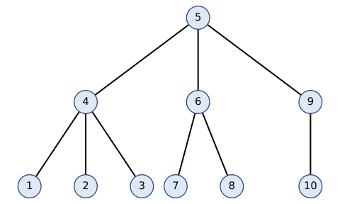
Encoding (Section 12.10.5, proof of Theorem 12.28): repeatedly delete the lowest-numbered leaf and record its neighbour, until two vertices remain.
| step | 1 | 2 | 3 | 4 | 5 | 6 | 7 | 8 |
|---|---|---|---|---|---|---|---|---|
| leaf deleted | 1 | 2 | 3 | 4 | 7 | 8 | 6 | 5 |
| neighbour | 4 | 4 | 4 | 5 | 6 | 6 | 5 | 9 |
The remaining vertices are \(9,10\).
Decoding: at each step join the smallest label that is neither already used nor present in the rest of the sequence to the first entry of the sequence, then delete that entry; finally join the last two unused labels.
| remaining sequence | smallest absent unused label | edge added |
|---|---|---|
| 4,4,4,5,6,6,5,9 | 1 | \(\{1,4\}\) |
| 4,4,5,6,6,5,9 | 2 | \(\{2,4\}\) |
| 4,5,6,6,5,9 | 3 | \(\{3,4\}\) |
| 5,6,6,5,9 | 4 | \(\{4,5\}\) |
| 6,6,5,9 | 7 | \(\{7,6\}\) |
| 6,5,9 | 8 | \(\{8,6\}\) |
| 5,9 | 6 | \(\{6,5\}\) |
| 9 | 5 | \(\{5,9\}\) |
| (empty) | unused: 9, 10 | \(\{9,10\}\) |
The nine edges recovered are exactly the edges of the original tree.
Exercise 12.43
Construct the tree corresponding to each of the following Prüfer sequences:
(1) \(1\,1\,3\,6\,6\,3\) (2) \(5\,5\,2\,8\,3\,3\,2\,2\,6\)
(1) The tree on \(\{1,\dots,8\}\) with edges
\begin{equation*} \{1,2\},\ \{1,4\},\ \{1,3\},\ \{5,6\},\ \{6,7\},\ \{3,6\},\ \{3,8\}. \end{equation*}
The sequence has length \(6\), so \(n=8\), and the labels missing from it give the starting leaf list \(\{2,4,5,7,8\}\). Run the decoding algorithm in the proof of Theorem 12.28 (Section 12.10.5: pair the first entry \(p\) with the smallest leaf \(e\); when \(p\) no longer appears later in the sequence, \(p\) becomes a leaf):
| step | \(p\) | \(e\) | edge | leaf list after |
|---|---|---|---|---|
| 1 | 1 | 2 | \(\{2,1\}\) | \(\{4,5,7,8\}\) |
| 2 | 1 | 4 | \(\{4,1\}\) | \(\{1,5,7,8\}\) |
| 3 | 3 | 1 | \(\{1,3\}\) | \(\{5,7,8\}\) |
| 4 | 6 | 5 | \(\{5,6\}\) | \(\{7,8\}\) |
| 5 | 6 | 7 | \(\{7,6\}\) | \(\{6,8\}\) |
| 6 | 3 | 6 | \(\{6,3\}\) | \(\{3,8\}\) |
The two labels left over give the last edge, \(\{3,8\}\): vertex \(1\) is adjacent to \(2,4,3\), vertex \(6\) to \(5,7,3\), and vertex \(3\) to \(1,6,8\).
(2) The tree on \(\{1,\dots,11\}\) with edges
\begin{equation*} \begin{aligned} &\{1,5\},\ \{4,5\},\ \{2,5\},\ \{7,8\},\ \{3,8\},\\ &\{3,9\},\ \{2,3\},\ \{2,10\},\ \{2,6\},\ \{6,11\}. \end{aligned} \end{equation*}
The sequence has length \(9\), so \(n=11\), and the starting leaf list is \(\{1,4,7,9,10,11\}\):
| step | \(p\) | \(e\) | edge | leaf list after |
|---|---|---|---|---|
| 1 | 5 | 1 | \(\{1,5\}\) | \(\{4,7,9,10,11\}\) |
| 2 | 5 | 4 | \(\{4,5\}\) | \(\{5,7,9,10,11\}\) |
| 3 | 2 | 5 | \(\{5,2\}\) | \(\{7,9,10,11\}\) |
| 4 | 8 | 7 | \(\{7,8\}\) | \(\{8,9,10,11\}\) |
| 5 | 3 | 8 | \(\{8,3\}\) | \(\{9,10,11\}\) |
| 6 | 3 | 9 | \(\{9,3\}\) | \(\{3,10,11\}\) |
| 7 | 2 | 3 | \(\{3,2\}\) | \(\{10,11\}\) |
| 8 | 2 | 10 | \(\{10,2\}\) | \(\{2,11\}\) |
| 9 | 6 | 2 | \(\{2,6\}\) | \(\{6,11\}\) |
The last edge is \(\{6,11\}\): vertex \(2\) is adjacent to \(5,3,10,6\); vertex \(5\) carries the leaves \(1,4\); vertex \(3\) carries \(8\) and the leaf \(9\); vertex \(8\) carries the leaf \(7\); vertex \(6\) carries the leaf \(11\).
Backlinks (2)
1. Foundations of Data Science /words/library/books/foundations-of-data-science/
A. Blum, J. Hopcroft and R. Kannan, Foundations of Data Science, Cambridge University Press, 2020 (freely available draft of 4 January 2018). The mathematics behind modern data analysis: high-dimensional geometry, the SVD, random walks and Markov chains, machine learning theory, streaming and sampling algorithms, clustering, random graphs and topic models.
Worked solutions to all 373 end-of-chapter exercises live at Solutions to Blum, Hopcroft & Kannan’s Foundations of Data Science.
2. Books /words/library/books/
Here are the books that I have taken the time to create metadata and/or notes for.
Comments