Solutions to Chiang’s Networked Life
Solutions to all 100 homework problems (five per chapter, difficulty-starred, some deliberately open-ended) in Mung Chiang’s Networked Life: 20 Questions and Answers (Cambridge, 2012). Computational answers are worked as jupyter-python blocks with their committed results — numpy/scipy/networkx experiments you can re-run. Open-ended problems get a substantiated position argued from the chapter’s models rather than a hedge.
What makes CDMA work for my smartphone?
Problem 1.1 — Distributed power control
Distributed power control.
(a) Consider three pairs of transmitters and receivers in a cell, with the following channel gain matrix \(\mathbf{G}\) and noise of 0.1 mW for all the receivers. The target SIRs are also shown below.
\[ \mathbf{G} = \begin{bmatrix} 1 & 0.1 & 0.3 \\ 0.2 & 1 & 0.3 \\ 0.2 & 0.2 & 1 \end{bmatrix}, \qquad \gamma = \begin{bmatrix} 1 \\ 1.5 \\ 1 \end{bmatrix}. \]
With an initialization of all transmit powers at 1 mW, run DPC for ten iterations and plot the evolution of transmit powers and received SIRs. You can use any programming language, or even write the steps out by hand.
(b) Now suppose the power levels for logical links 1, 2, and 3 have converged to the equilibrium in (a). A new pair of transmitter and receiver, labeled as logical link 4, shows up in the same cell, with an initial transmit power of 1 mW and demands a target SIR of 1. The new channel gain matrix is shown below.
\[ \mathbf{G} = \begin{bmatrix} 1 & 0.1 & 0.3 & 0.1 \\ 0.2 & 1 & 0.3 & 0.1 \\ 0.2 & 0.2 & 1 & 0.1 \\ 0.1 & 0.1 & 0.1 & 1 \end{bmatrix}. \]
Similarly to what you did in (a), show what happens in the next ten timeslots. What happens at the new equilibrium? (difficulty: \(\star\))
The SIR at receiver \(i\) is equation (1.1) and the DPC update is equation (1.2):
\begin{equation*} \mathrm{SIR}_i(\mathbf{p}) = \frac{G_{ii} p_i}{\sum_{j \neq i} G_{ij} p_j + n_i}, \qquad p_i[t+1] = \frac{\gamma_i}{\mathrm{SIR}_i[t]}\, p_i[t] , \end{equation*}
so row \(i\) of \(\mathbf{G}\) collects everything landing on receiver \(i\). In the matrix form of Section 1.4.1 — \(\mathbf{D} = \mathrm{diag}(\gamma)\), \(F_{ij} = G_{ij}/G_{ii}\) for \(i \neq j\), \(F_{ii} = 0\), \(v_i = \gamma_i n_i/G_{ii}\) — the targets read \(\mathbf{p} \ge \mathbf{DFp} + \mathbf{v}\), with power-minimal solution \(\mathbf{p}^\ast = (\mathbf{I}-\mathbf{DF})^{-1}\mathbf{v}\), reached by DPC whenever \(\rho(\mathbf{DF}) < 1\).
Part (a).
import numpy as np
np.set_printoptions(precision=4, suppress=True)

def sir(p, G, n):
    signal = np.diag(G) * p
    return signal / (G @ p - signal + n)

def dpc(G, gamma, n, p0, T=10):
    p = p0.copy()
    P, S = [p.copy()], [sir(p, G, n)]
    for _ in range(T):
        p = gamma / sir(p, G, n) * p
        P.append(p.copy())
        S.append(sir(p, G, n))
    return np.array(P), np.array(S)

def fixed_point(G, gamma, n):
    F = G / np.diag(G)[:, None]
    np.fill_diagonal(F, 0.0)
    DF = np.diag(gamma) @ F
    v = gamma * n / np.diag(G)
    rho = max(abs(np.linalg.eigvals(DF)))
    return rho, np.linalg.solve(np.eye(len(gamma)) - DF, v)

G3 = np.array([[1.0, 0.1, 0.3],
               [0.2, 1.0, 0.3],
               [0.2, 0.2, 1.0]])
g3 = np.array([1.0, 1.5, 1.0])
n3 = 0.1 * np.ones(3)

P3, S3 = dpc(G3, g3, n3, np.ones(3))
for t in range(11):
    print(f"t={t:2d}  p={P3[t]}  SIR={S3[t]}")

rho3, p3star = fixed_point(G3, g3, n3)
print(f"rho(DF) = {rho3:.6f}")
print("p*      =", p3star)
print("SIR(p*) =", sir(p3star, G3, n3))
t= 0  p=[1. 1. 1.]  SIR=[2.     1.6667 2.    ]
t= 1  p=[0.5 0.9 0.5]  SIR=[1.4706 2.5714 1.3158]
t= 2  p=[0.34  0.525 0.38 ]  SIR=[1.2758 1.8617 1.3919]
t= 3  p=[0.2665 0.423  0.273 ]  SIR=[1.1887 1.7985 1.1475]
t= 4  p=[0.2242 0.3528 0.2379]  SIR=[1.0849 1.6317 1.1045]
t= 5  p=[0.2066 0.3243 0.2154]  SIR=[1.0487 1.5747 1.0447]
t= 6  p=[0.1971 0.3089 0.2062]  SIR=[1.0223 1.5349 1.0248]
t= 7  p=[0.1928 0.3019 0.2012]  SIR=[1.0116 1.5178 1.0114]
t= 8  p=[0.1905 0.2984 0.1989]  SIR=[1.0055 1.5085 1.0058]
t= 9  p=[0.1895 0.2967 0.1978]  SIR=[1.0027 1.5042 1.0028]
t=10  p=[0.189  0.2959 0.1972]  SIR=[1.0013 1.502  1.0014]
rho(DF) = 0.485410
p*      = [0.1885 0.2951 0.1967]
SIR(p*) = [1.  1.5 1. ]
Hand-checking the first slot: at \(\mathbf{p}[0] = (1,1,1)\),
\begin{equation*} \mathrm{SIR}[0] = \left( \tfrac{1}{0.5},\ \tfrac{1}{0.6},\ \tfrac{1}{0.5} \right) = \left( 2,\ \tfrac{5}{3},\ 2 \right) , \end{equation*}
so \(\mathbf{p}[1] = (0.5,\ 0.9,\ 0.5)\), matching row \(t=1\). Everyone starts above target, so the first move is a coordinated retreat; the powers then fall monotonically to \(\mathbf{p}^\ast\) from above and the SIRs settle onto target from above from \(t=2\) on (links 2 and 3 overshoot once, each link’s retreat being partly cancelled by the others’ retreating in the same slot). The error decays geometrically at rate \(\rho(\mathbf{DF}) = 0.4854\) — the gap \(p_1[t] - p_1^\ast\) runs \(0.0020,\ 0.0010,\ 0.0005\) — so after ten slots the SIRs are within \(0.2\%\) of the power-minimal equilibrium
\[ \mathbf{p}^\ast = (0.1885,\ 0.2951,\ 0.1967)\ \text{mW} . \]
import matplotlib.pyplot as plt

def plot_run(P, S, gamma, title, fname):
    T = np.arange(P.shape[0])
    fig, ax = plt.subplots(1, 2, figsize=(10, 3.6))
    for i in range(P.shape[1]):
        ax[0].plot(T, P[:, i], marker='o', ms=3, label=f"link {i+1}")
        ax[1].plot(T, S[:, i], marker='o', ms=3, label=f"link {i+1}")
    for gv in gamma:
        ax[1].axhline(gv, ls=':', lw=0.8, color='gray')
    ax[0].set_xlabel("iteration t"); ax[0].set_ylabel("transmit power (mW)")
    ax[1].set_xlabel("iteration t"); ax[1].set_ylabel("received SIR")
    ax[0].legend(fontsize=8); ax[1].legend(fontsize=8)
    fig.suptitle(title); fig.tight_layout()
    fig.savefig(fname, dpi=150, bbox_inches='tight')
    plt.close(fig)

plot_run(P3, S3, g3, "DPC, three links, targets (1, 1.5, 1)",
         'nl-ch01-dpc-three-links.svg')
print("saved nl-ch01-dpc-three-links.svg")
saved nl-ch01-dpc-three-links.svg
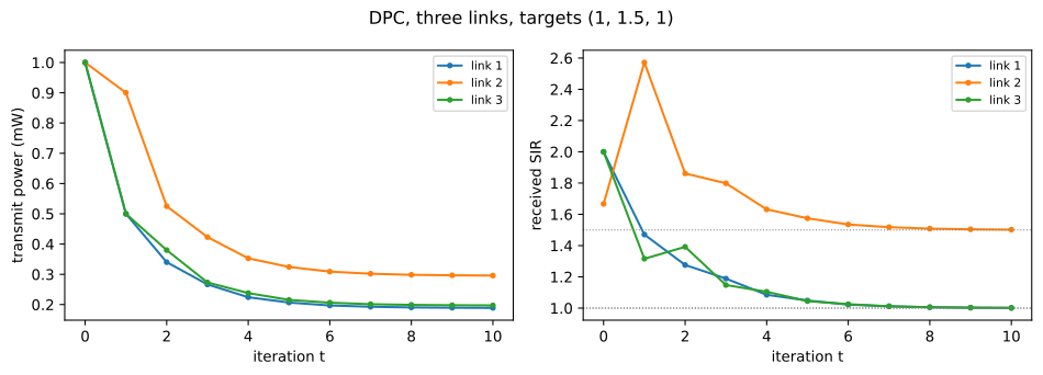
Part (a). Left: transmit powers over ten DPC iterations from a 1 mW start. Right: received SIRs converging to the dotted targets 1, 1.5, 1.
Part (b). Links 1–3 start at \(\mathbf{p}^\ast\) from (a); link 4 barges in at 1 mW with \(\gamma_4 = 1\).
G4 = np.array([[1.0, 0.1, 0.3, 0.1],
               [0.2, 1.0, 0.3, 0.1],
               [0.2, 0.2, 1.0, 0.1],
               [0.1, 0.1, 0.1, 1.0]])
g4 = np.array([1.0, 1.5, 1.0, 1.0])
n4 = 0.1 * np.ones(4)

p0 = np.concatenate([p3star, [1.0]])
P4, S4 = dpc(G4, g4, n4, p0)
for t in range(11):
    print(f"t={t:2d}  p={P4[t]}  SIR={S4[t]}")

rho4, p4star = fixed_point(G4, g4, n4)
print(f"rho(DF) = {rho4:.6f}")
print("p*      =", p4star)
print("power increase on links 1-3 (%):",
      np.round(100 * (p4star[:3] / p3star - 1), 2))

plot_run(P4, S4, g4, "DPC after link 4 joins at 1 mW",
         'nl-ch01-dpc-new-link.svg')
print("saved nl-ch01-dpc-new-link.svg")
t= 0  p=[0.1885 0.2951 0.1967 1.    ]  SIR=[0.6534 0.9945 0.663  5.9512]
t= 1  p=[0.2885 0.4451 0.2967 0.168 ]  SIR=[1.1526 1.689  1.126  0.8276]
t= 2  p=[0.2503 0.3953 0.2635 0.203 ]  SIR=[1.0479 1.5848 1.0565 1.0635]
t= 3  p=[0.2389 0.3741 0.2494 0.1909]  SIR=[1.0327 1.548  1.032  1.0251]
t= 4  p=[0.2313 0.3625 0.2417 0.1862]  SIR=[1.0173 1.5271 1.0181 1.0146]
t= 5  p=[0.2274 0.3561 0.2374 0.1836]  SIR=[1.0098 1.515  1.01   1.0081]
t= 6  p=[0.2252 0.3526 0.2351 0.1821]  SIR=[1.0054 1.5083 1.0055 1.0045]
t= 7  p=[0.224  0.3506 0.2338 0.1813]  SIR=[1.003  1.5046 1.003  1.0025]
t= 8  p=[0.2233 0.3496 0.2331 0.1808]  SIR=[1.0016 1.5025 1.0017 1.0013]
t= 9  p=[0.223  0.349  0.2327 0.1806]  SIR=[1.0009 1.5014 1.0009 1.0007]
t=10  p=[0.2228 0.3487 0.2325 0.1805]  SIR=[1.0005 1.5008 1.0005 1.0004]
rho(DF) = 0.549169
p*      = [0.2225 0.3483 0.2322 0.1803]
power increase on links 1-3 (%): [18.03 18.03 18.03]
saved nl-ch01-dpc-new-link.svg
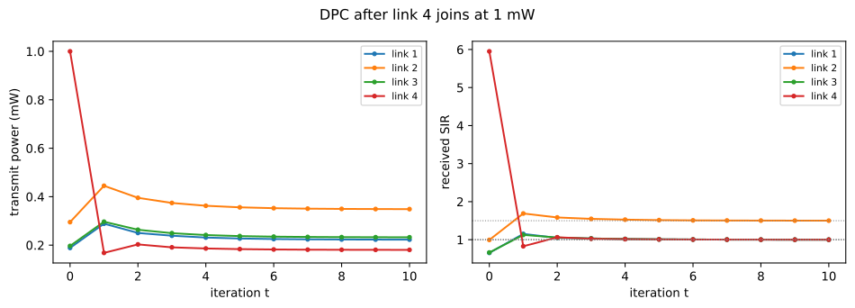
Part (b). Link 4 arrives at 1 mW and is immediately throttled from 1 mW to 0.168 mW; the three incumbents raise power by 18% and everyone re-converges to target within about five slots.
The near-far problem in miniature, then its cure. At \(t=0\) the newcomer transmits at 1 mW, several times what anyone else uses, so it enjoys \(\mathrm{SIR}_4 = 5.95\) while knocking all three incumbents below target \((0.65,\ 0.99,\ 0.66)\). One slot fixes it: link 4 cuts to \(0.168\) mW while links 1–3 push up, and from \(t=2\) everything settles monotonically to
\[ \mathbf{p}^\ast = (0.2225,\ 0.3483,\ 0.2322,\ 0.1803)\ \text{mW} \]
with all four SIRs at target; \(\rho(\mathbf{DF})\) rises only from \(0.485\) to \(0.549\), so the system stays comfortably feasible.
At the new equilibrium links 1–3 each hold exactly 18.03% more power, which is no accident: \(G_{i4} = 0.1 = n_i\) and \(G_{ii} = 1\) for \(i \le 3\), so the interference link 4 adds to row \(i\) of equation (1.4) is
\begin{equation*} \gamma_i \frac{G_{i4}}{G_{ii}}\, p_4^\ast = \gamma_i (0.1) p_4^\ast = v_i\, p_4^\ast . \end{equation*}
The three-link right-hand side therefore becomes \((1 + p_4^\ast)\mathbf{v}\), and by linearity of \((\mathbf{I}-\mathbf{D}_3\mathbf{F}_3)^{-1}\) the solution scales by \(1 + 0.1803\). To the incumbents link 4 is indistinguishable from an 18% higher noise floor: the negative externality of Section 1.2.3 collected as a power tax.
Problem 1.2 — Power control infeasibility
Power control infeasibility.
Consider a three-link cell with the link gains \(G_{ij}\) shown below. The receivers request \(\gamma_1 = 1\), \(\gamma_2 = 2\), and \(\gamma_3 = 1\). The noise \(n_i = 0.1\) for all \(i\).
\[ \mathbf{G} = \begin{bmatrix} 1 & 0.5 & 0.5 \\ 0.5 & 1 & 0.5 \\ 0.5 & 0.5 & 1 \end{bmatrix}. \]
Prove this set of target SIRs is infeasible. (difficulty: \(\star\star\))
No \(\mathbf{p} \ge \mathbf{0}\) meets all three targets: adding the three constraints leaves \(0 \ge 0.4\). In detail, suppose such a \(\mathbf{p}\) existed. Equation (1.4) writes \(\mathrm{SIR}_i \ge \gamma_i\) as \(p_i \ge \gamma_i \sum_{j \neq i} (G_{ij}/G_{ii}) p_j + \gamma_i n_i/G_{ii}\), and with \(G_{ii} = 1\), \(G_{ij} = 0.5\), \(n_i = 0.1\) this reads
\[ p_1 \ \ge\ 0.5 p_2 + 0.5 p_3 + 0.1, \] \[ p_2 \ \ge\ 2(0.5 p_1 + 0.5 p_3) + 2(0.1) \ =\ p_1 + p_3 + 0.2, \] \[ p_3 \ \ge\ 0.5 p_1 + 0.5 p_2 + 0.1. \]
Summing the three and cancelling \(p_1 + p_2 + p_3\) from both sides leaves
\[ 0 \ \ge\ 0.5 p_1 + 0.5 p_3 + 0.4 \ \ge\ 0.4 \ >\ 0 , \]
using \(p_1, p_3 \ge 0\). Contradiction, so \(\gamma = (1,2,1)\) is infeasible. \(\blacksquare\)
Method (2): the spectral radius. Section 1.4.1 gives the Perron–Frobenius test \(\rho(\mathbf{DF}) < 1\) for feasibility; for this nonnegative \(\mathbf{DF}\) with \(\mathbf{v} > \mathbf{0}\) the converse holds too, so \(\rho(\mathbf{DF}) > 1\) proves infeasibility rather than merely failing a sufficient condition. With \(\mathbf{D} = \mathrm{diag}(1,2,1)\) and \(F_{ij} = 0.5\) off-diagonal,
\[ \mathbf{DF} = \begin{bmatrix} 0 & 0.5 & 0.5 \\ 1 & 0 & 1 \\ 0.5 & 0.5 & 0 \end{bmatrix}. \]
Its characteristic polynomial \(\lambda^3 - \tfrac{5}{4}\lambda - \tfrac{1}{2}\) factors as \((\lambda + \tfrac{1}{2})(\lambda^2 - \tfrac{1}{2}\lambda - 1)\), so the Perron root is
\[ \rho(\mathbf{DF}) = \frac{1 + \sqrt{17}}{4} \approx 1.2808 \ >\ 1 , \]
whence \(\sum_k (\mathbf{DF})^k\) diverges, \((\mathbf{I}-\mathbf{DF})^{-1}\) is not nonnegative, and no \(\mathbf{p}^\ast\) exists.
import numpy as np
np.set_printoptions(precision=4, suppress=True)

G = np.array([[1.0, 0.5, 0.5],
              [0.5, 1.0, 0.5],
              [0.5, 0.5, 1.0]])
gam = np.array([1.0, 2.0, 1.0])
n = 0.1 * np.ones(3)

F = G / np.diag(G)[:, None]
np.fill_diagonal(F, 0.0)
DF = np.diag(gam) @ F
ev = np.linalg.eigvals(DF)
print("eigenvalues of DF:", np.sort(ev.real))
print("rho(DF)          =", round(max(abs(ev)), 6))
print("(1+sqrt(17))/4   =", round((1 + np.sqrt(17)) / 4, 6))

def sir(p, G, n):
    s = np.diag(G) * p
    return s / (G @ p - s + n)

p = np.ones(3)
for t in range(1, 41):
    p = gam / sir(p, G, n) * p
    if t in (1, 2, 5, 10, 20, 40):
        print(f"t={t:3d}  p={p}  SIR={sir(p, G, n)}")

from scipy.optimize import linprog
res = linprog(c=np.ones(3), A_ub=-(np.eye(3) - DF),
              b_ub=-(gam * n / np.diag(G)), bounds=[(0, None)] * 3)
print("LP of problem (1.5):", res.message)
eigenvalues of DF: [-0.7808 -0.5     1.2808]
rho(DF)          = 1.280776
(1+sqrt(17))/4   = 1.280776
t=  1  p=[1.1 2.2 1.1]  SIR=[0.6286 1.8333 0.6286]
t=  2  p=[1.75 2.4  1.75]  SIR=[0.8046 1.2973 0.8046]
t=  5  p=[3.8937 6.275  3.8937]  SIR=[0.7511 1.5712 0.7511]
t= 10  p=[14.5521 22.6992 14.5521]  SIR=[0.7771 1.5492 0.7771]
t= 20  p=[177.0563 276.5033 177.0563]  SIR=[0.7804 1.5608 0.7804]
t= 40  p=[25035.0479 39093.5741 25035.0479]  SIR=[0.7808 1.5615 0.7808]
LP of problem (1.5): The problem is infeasible. (HiGHS Status 8: model_status is Infeasible; primal_status is At lower/fixed bound)
The transmit-power arms race of Section 1.1: powers grow at rate \(1.2808\) per slot, four orders of magnitude by \(t=40\), while the SIRs flatline at \(\gamma_i/\rho(\mathbf{DF}) = (0.781, 1.562, 0.781)\) — the power vector aligns with the Perron eigenvector, the noise becomes negligible, and every link falls short by the same factor \(\rho\).
Problem 1.3 — A zero-sum game
A zero-sum game.
In the following two-user game, the payoffs of users Alice and Bob are exactly negative of each other in all the combinations of strategies (a,a), (a,b), (b,a), (b,b). This models an extreme case of competition, and is called a zero-sum game. Is there any pure strategy equilibrium? How many are there?
Alice picks the row, Bob picks the column; each cell lists (Alice’s payoff, Bob’s payoff):
| a | b | |
|---|---|---|
| a | (2, -2) | (3, -3) |
| b | (3, -3) | (4, -4) |
(difficulty: \(\star\))
Yes, and there is exactly one: \((b, a)\), with payoffs \((3, -3)\).
Both players hold a strictly dominant strategy, so the best-response condition of Section 1.2.3 pins down one cell. Alice reads down columns and row \(b\) wins both (\(3 > 2\) and \(4 > 3\)); Bob, whose payoffs are the negatives, is minimizing Alice’s number and column \(a\) wins both rows (\(-2 > -3\) and \(-3 > -4\)). Their intersection is \((b,a)\), and iterated elimination of the strictly dominated row \(a\) and column \(b\) leaves that single cell, so it is the only one.
Method (2): saddle point. Alice’s row minima are \(2\) and \(3\), so her maximin is \(3\); Bob’s column maxima are \(3\) and \(4\), so his minimax is \(3\). Maximin and minimax agree, so \(3\) is the value of the game and the entry realizing it, \((b,a)\), is its unique saddle point — largest in its column, smallest in its row.
import numpy as np
import itertools

S = ['a', 'b']
UA = np.array([[2.0, 3.0],
               [3.0, 4.0]])
UB = -UA

eq = []
for i, j in itertools.product(range(2), range(2)):
    alice_ok = all(UA[i, j] >= UA[k, j] for k in range(2))
    bob_ok = all(UB[i, j] >= UB[i, l] for l in range(2))
    print(f"({S[i]},{S[j]}) payoff ({UA[i,j]:.0f},{UB[i,j]:.0f})"
          f"  Alice best-response: {alice_ok}   Bob best-response: {bob_ok}")
    if alice_ok and bob_ok:
        eq.append((S[i], S[j]))
print("pure Nash equilibria:", eq, " count =", len(eq))
print("maximin for Alice =", UA.min(axis=1).max())
print("minimax for Bob   =", UA.max(axis=0).min())
(a,a) payoff (2,-2)  Alice best-response: False   Bob best-response: True
(a,b) payoff (3,-3)  Alice best-response: False   Bob best-response: False
(b,a) payoff (3,-3)  Alice best-response: True   Bob best-response: True
(b,b) payoff (4,-4)  Alice best-response: True   Bob best-response: False
pure Nash equilibria: [('b', 'a')]  count = 1
maximin for Alice = 3.0
minimax for Bob   = 3.0
Problem 1.4 — Mechanism design
Mechanism design.
Consider the game below. There are two players, Alice and Bob, each with two strategies, and the payoffs are shown below. Consider only pure strategy equilibria.
Alice picks the row, Bob picks the column; each cell lists (Alice’s payoff, Bob’s payoff):
| a | b | |
|---|---|---|
| a | (0, 2) | (2, 0) |
| b | (6, 0) | (3, 2) |
(a) Is there a Nash equilibrium, and, if so, what is it?
(b) We want to make this game a “better” one. What entries in the table would you change to make the resulting Nash equilibrium unique and socially optimal?
This is an example of mechanism design: change the game so as to induce movement of players to a desirable equilibrium. We will see a lot more of mechanism design in future chapters. (difficulty: \(\star\star\))
Part (a). There is exactly one pure Nash equilibrium: \((b, b)\), with payoffs \((3, 2)\).
Row \(b\) strictly dominates for Alice (\(6 > 0\) against Bob’s \(a\), \(3 > 2\) against his \(b\)). Bob has no dominant strategy but wants to match Alice, so against her \(b\) he answers \(b\) (\(2 > 0\)); the other three cells die to one deviation each. The equilibrium is not socially optimal: the cell sums in the \(\sum_i U_i\) sense of Section 1.2.3 are \(2, 2, 6, 5\) for \((a,a), (a,b), (b,a), (b,b)\), so the optimum is \((b,a)\) at \(6\) while play lands on \((b,b)\) at \(5\). The gap is a smaller pie rather than a Pareto failure — moving to \((b,a)\) gains Alice \(3\) and costs Bob \(2\), and \((b,b)\) is itself Pareto optimal — so this is Table 1.1’s pathology in mild form.
Part (b). Raise Bob’s payoff at \((b,a)\) from \(0\) to \(3\); any value strictly above \(2\) serves. The table becomes
| a | b | |
|---|---|---|
| a | (0, 2) | (2, 0) |
| b | (6, 3) | (3, 2) |
Alice’s payoffs are untouched, so row \(b\) still strictly dominates and both top cells die; Bob now strictly prefers \(a\) to \(b\) in row \(b\) (\(3 > 2\)), leaving \((b,a)\) as the unique equilibrium, with welfare \(6 + 3 = 9\) against \(2\), \(2\), \(5\) elsewhere. So it is uniquely stable, socially optimal, and Pareto optimal.
The edit pays Bob rather than distorting Alice because the externality is one-sided: her dominant \(b\) already creates the surplus, and the only obstacle is that Bob, on whom none of it falls, has no reason to sit in column \(a\). Subsidizing him \(3\) conditional on \((b,a)\) is the “internalize the externality” move of Section 1.1. Punishing Bob at \((b,b)\) instead would also relocate the equilibrium but leaves the social optimum at \(6\) rather than \(9\); both are verified below.
import numpy as np
import itertools

S = ['a', 'b']

def analyse(UA, UB, label):
    print(f"--- {label}")
    eq = []
    for i, j in itertools.product(range(2), range(2)):
        ok_a = all(UA[i, j] >= UA[k, j] for k in range(2))
        ok_b = all(UB[i, j] >= UB[i, l] for l in range(2))
        tag = "  <-- NASH" if (ok_a and ok_b) else ""
        print(f"({S[i]},{S[j]}) = ({UA[i,j]:.0f},{UB[i,j]:.0f})"
              f"  sum={UA[i,j]+UB[i,j]:.0f}{tag}")
        if ok_a and ok_b:
            eq.append((S[i], S[j]))
    tot = UA + UB
    best = np.unravel_index(np.argmax(tot), tot.shape)
    print("pure Nash:", eq)
    print("socially optimal cell:", (S[best[0]], S[best[1]]),
          "with sum", tot[best])
    print("Nash is unique and socially optimal:",
          len(eq) == 1 and eq[0] == (S[best[0]], S[best[1]]))

UA = np.array([[0.0, 2.0], [6.0, 3.0]])
UB = np.array([[2.0, 0.0], [0.0, 2.0]])
analyse(UA, UB, "original game")

UB2 = UB.copy(); UB2[1, 0] = 3.0
analyse(UA, UB2, "modified: Bob's payoff at (b,a) raised 0 -> 3")

UB3 = UB.copy(); UB3[1, 1] = -1.0
analyse(UA, UB3, "alternative: Bob's payoff at (b,b) lowered 2 -> -1")
--- original game
(a,a) = (0,2)  sum=2
(a,b) = (2,0)  sum=2
(b,a) = (6,0)  sum=6
(b,b) = (3,2)  sum=5  <-- NASH
pure Nash: [('b', 'b')]
socially optimal cell: ('b', 'a') with sum 6.0
Nash is unique and socially optimal: False
--- modified: Bob's payoff at (b,a) raised 0 -> 3
(a,a) = (0,2)  sum=2
(a,b) = (2,0)  sum=2
(b,a) = (6,3)  sum=9  <-- NASH
(b,b) = (3,2)  sum=5
pure Nash: [('b', 'a')]
socially optimal cell: ('b', 'a') with sum 9.0
Nash is unique and socially optimal: True
--- alternative: Bob's payoff at (b,b) lowered 2 -> -1
(a,a) = (0,2)  sum=2
(a,b) = (2,0)  sum=2
(b,a) = (6,0)  sum=6  <-- NASH
(b,b) = (3,-1)  sum=2
pure Nash: [('b', 'a')]
socially optimal cell: ('b', 'a') with sum 6.0
Nash is unique and socially optimal: True
Problem 1.5 — Repeating prisoner’s dilemma
Repeating prisoner’s dilemma.
The stage game is the prisoner’s dilemma of Table 1.1. Player A picks the row, player B picks the column, and each cell gives (A’s payoff, B’s payoff) as negative years served:
| Not Confess | Confess | |
|---|---|---|
| Not Confess | (-1, -1) | (-5, 0) |
| Confess | (0, -5) | (-3, -3) |
(a) Suppose the two prisoners know that they will somehow be caught in the same situation five more times in future years. What will each prisoner’s strategy be in choosing between confession and no confession?
(b) Suppose the two prisoners have infinite lifetimes, and there is always a 90% chance that they will be caught in the same situation after each round of this game. What will each prisoner’s strategy be now? (difficulty: \(\star\star\star\))
Both confess in all six rounds in (a); both cooperate in every round in (b). The stage game is unchanged — only the shadow of the future. Write \(C\) for Not Confess and \(D\) for Confess; Table 1.1 gives \(u(D,C) = 0 > u(C,C) = -1 > u(D,D) = -3 > u(C,D) = -5\), so \(D\) is strictly dominant and \((D,D)\) is the unique stage equilibrium.
Part (a). The horizon \(T = 6\) is finite and commonly known, so run backward induction. Round 6 has no future to influence and is literally the one-shot game, where \(D\) strictly dominates; round 5 therefore faces a constant continuation payoff, so maximizing the total reduces to the round-5 stage payoff and \(D\) dominates again; the same step runs back through rounds 4 to 1. Every elimination uses strict dominance, so confessing in all six rounds is the unique subgame-perfect equilibrium and indeed the unique Nash outcome: \(-18\) years each, against the \(-6\) of mutual cooperation.
The mechanism that fails is worth naming. Cooperation in a repeated game must be enforced by the threat of future punishment, but a threat only bites if there is a future left to punish in. In the last round there is none, so cooperation collapses there; and once it collapses there, the second-to-last round has no enforceable future either, and the collapse unravels all the way back to round 1. The code below runs that unravelling explicitly as iterated best response, starting from an opponent who would happily cooperate all six rounds.
import numpy as np

# stage payoffs to me, keyed (my move, other move); C = Not Confess, D = Confess
u = {('C', 'C'): -1, ('C', 'D'): -5, ('D', 'C'): 0, ('D', 'D'): -3}

for other in ['C', 'D']:
    print(f"other plays {other}:  I cooperate -> {u[('C', other)]},"
          f"  I confess -> {u[('D', other)]}"
          f"   => confess strictly better: {u[('D', other)] > u[('C', other)]}")

T = 6
print(f"T = {T} rounds:  both always confess -> {T * u[('D','D')]} each;"
      f"  both always cooperate -> {T * u[('C','C')]} each")

def best_response(T, k):
    # opponent cooperates in rounds 0..k-1 unless I have ever defected,
    # then confesses forever.  Return my optimal action string and payoff.
    V = {(T, True): 0.0, (T, False): 0.0}
    act = {}
    for t in range(T - 1, -1, -1):
        V[(t, True)] = u[('D', 'D')] + V[(t + 1, True)]     # already punished
        if t < k:
            coop = u[('C', 'C')] + V[(t + 1, False)]
            defect = u[('D', 'C')] + V[(t + 1, True)]
            V[(t, False)] = max(coop, defect)
            act[t] = 'C' if coop > defect else 'D'
        else:
            V[(t, False)] = u[('D', 'D')] + V[(t + 1, True)]
            act[t] = 'D'
    return ''.join(act[t] for t in range(T)), V[(0, False)]

k = T
for r in range(1, 8):
    path, val = best_response(T, k)
    print(f"round {r} of iterated best response: opponent cooperates for {k} slots"
          f"  ->  my best reply {path} (payoff {val:.0f})")
    k_new = path.find('D') if 'D' in path else T
    if k_new == k:
        print("fixed point reached")
        break
    k = k_new
other plays C:  I cooperate -> -1,  I confess -> 0   => confess strictly better: True
other plays D:  I cooperate -> -5,  I confess -> -3   => confess strictly better: True
T = 6 rounds:  both always confess -> -18 each;  both always cooperate -> -6 each
round 1 of iterated best response: opponent cooperates for 6 slots  ->  my best reply CCCCCD (payoff -5)
round 2 of iterated best response: opponent cooperates for 5 slots  ->  my best reply CCCCDD (payoff -7)
round 3 of iterated best response: opponent cooperates for 4 slots  ->  my best reply CCCDDD (payoff -9)
round 4 of iterated best response: opponent cooperates for 3 slots  ->  my best reply CCDDDD (payoff -11)
round 5 of iterated best response: opponent cooperates for 2 slots  ->  my best reply CDDDDD (payoff -13)
round 6 of iterated best response: opponent cooperates for 1 slots  ->  my best reply DDDDDD (payoff -15)
round 7 of iterated best response: opponent cooperates for 0 slots  ->  my best reply DDDDDD (payoff -18)
fixed point reached
Each pass strips one more round of cooperation off the tail, the first defection walking back from round 6 to round 1; against a partner who really would cooperate all six rounds the best reply is to cooperate five times and defect in the last, and that single crack is what the edifice falls through.
Part (b). Play now continues with probability \(\delta = 0.9\) after each round, so the expected payoff of \(\{u_t\}\) is \(\sum_{t \ge 0}\delta^t u_t\) and there is no commonly known last round: the game ends almost surely, yet no player ever occupies a node known to be terminal, so backward induction has nothing to unravel from. Take grim trigger — play \(C\) while all past play was \(C\), else \(D\) forever — and apply the one-shot deviation principle:
\begin{equation*} V_C = \sum_{t \ge 0} \delta^t (-1) = \frac{-1}{1-\delta} = -10 , \qquad V_D = 0 + \sum_{t \ge 1} \delta^t (-3) = \frac{-3\delta}{1-\delta} = -27 . \end{equation*}
Since \(1 - \delta > 0\), \(V_C \ge V_D\) is just \(-1 \ge -3\delta\), i.e. \(\delta \ge 1/3\), comfortably met. The punishment is credible because \((D,D)\) forever is itself an equilibrium of every subgame, so grim trigger is subgame perfect.
Milder tit-for-tat — play \(C\), thereafter copy the opponent’s last move — sustains cooperation under a weaker condition. Deviating once and returning to \(C\) pays \(0\) now, \(u(C,D) = -5\) under retaliation, then \(-1\) forever:
\begin{equation*} 0 - 5\delta - \frac{\delta^2}{1-\delta} \ \le\ \frac{-1}{1-\delta} \iff (4\delta - 1)(\delta - 1) \le 0 \iff \delta \ge \tfrac{1}{4} , \end{equation*}
again satisfied with room to spare: \(-12.6\) against \(-10\).
def payoffs(d):
    coop = -1 / (1 - d)
    grim_dev = 0 + d * (-3) / (1 - d)
    tft_dev = 0 + d * (-5) + d**2 * (-1) / (1 - d)
    return coop, grim_dev, tft_dev

for d in [0.20, 0.25, 1/3, 0.50, 0.90]:
    c, g, t = payoffs(d)
    print(f"delta={d:.4f}  cooperate={c:8.3f}"
          f"   deviate vs grim={g:8.3f} ({'holds' if c >= g else 'FAILS'})"
          f"   deviate vs TFT={t:8.3f} ({'holds' if c >= t else 'FAILS'})")

def threshold(idx):
    lo, hi = 1e-9, 1 - 1e-9
    for _ in range(200):
        mid = 0.5 * (lo + hi)
        p = payoffs(mid)
        if p[0] >= p[idx]:
            hi = mid
        else:
            lo = mid
    return hi

print("grim trigger threshold =", round(threshold(1), 6), " (1/3 =", round(1/3, 6), ")")
print("tit-for-tat  threshold =", round(threshold(2), 6), " (1/4 = 0.25 )")
print("expected number of rounds at delta=0.9 =", 1 / (1 - 0.9))
delta=0.2000  cooperate=  -1.250   deviate vs grim=  -0.750 (FAILS)   deviate vs TFT=  -1.050 (FAILS)
delta=0.2500  cooperate=  -1.333   deviate vs grim=  -1.000 (FAILS)   deviate vs TFT=  -1.333 (holds)
delta=0.3333  cooperate=  -1.500   deviate vs grim=  -1.500 (holds)   deviate vs TFT=  -1.833 (holds)
delta=0.5000  cooperate=  -2.000   deviate vs grim=  -3.000 (holds)   deviate vs TFT=  -3.000 (holds)
delta=0.9000  cooperate= -10.000   deviate vs grim= -27.000 (holds)   deviate vs TFT= -12.600 (holds)
grim trigger threshold = 0.333333  (1/3 = 0.333333 )
tit-for-tat  threshold = 0.25  (1/4 = 0.25 )
expected number of rounds at delta=0.9 = 10.000000000000002
Cooperation is not the only equilibrium here — always-confess survives, and by the folk theorem so does essentially any average payoff between \(-3\) and \(-1\) — so equilibrium analysis alone does not force it. I predict it anyway: \(\delta = 0.9\) clears the grim threshold by a factor of \(2.7\) and the tit-for-tat threshold by \(3.6\), so the conclusion survives large errors in the payoffs or in the players’ estimate of \(\delta\), and cooperation Pareto-dominates always-confess at \(-10\) against \(-30\) expected years each, which makes it the outcome both players want to coordinate on.
How does Google sell ad spaces?
Problem 2.1 — A simple ad space auction
A simple ad space auction. Three advertisers (1, 2, 3) bid for two ad spaces (A, B). The average revenues per click are $6, $4, $3 for the bidders, respectively, and the clickthrough rate of the ad spaces are 500, 300 clicks per hour respectively.
(a) Draw the bipartite graph with nodes indicating advertisers/ad spaces and edges indicating values per hour. Indicate the maximum matching with bold lines.
(b) Assume a GSP auction with truthful bidding, what is the result of the auction in terms of the allocation, the prices charged, and the payoffs received? (difficulty: \(\star\))
(a) The bipartite graph.
Edge weights are the products \(v_{ij} = R_i C_j\) of Section 2.2.4, i.e. the outer product of \(R = (6, 4, 3)\) dollars per click with \(C = (500, 300)\) clicks per hour.
import itertools
import numpy as np

R = np.array([6.0, 4.0, 3.0])          # revenue per click, bidders 1,2,3
C = np.array([500.0, 300.0])           # clickthrough rates, spaces A,B
V = np.outer(R, C)                     # v_ij = R_i * C_j, value per hour
print("valuation matrix (rows = bidders 1-3, cols = spaces A,B):")
print(V)

best, bestw = None, -1.0
for pair in itertools.permutations(range(3), 2):   # (bidder on A, bidder on B)
    w = V[pair[0], 0] + V[pair[1], 1]
    if w > bestw:
        bestw, best = w, pair
print("max-weight matching: bidder %d -> A, bidder %d -> B, weight %.0f/hr"
      % (best[0]+1, best[1]+1, bestw))
valuation matrix (rows = bidders 1-3, cols = spaces A,B):
[[3000. 1800.]
 [2000. 1200.]
 [1500.  900.]]
max-weight matching: bidder 1 -> A, bidder 2 -> B, weight 4200/hr
So the graph carries bidders \(\{1,2,3\}\) on the left, spaces \(\{A,B\}\) on the right, and all six edges, \[ v_{1A}=3000,\quad v_{1B}=1800,\quad v_{2A}=2000, \] \[ v_{2B}=1200,\quad v_{3A}=1500,\quad v_{3B}=900 \] dollars per hour. The valuation matrix has rank one, so the maximum-weight matching is the horizontal one of Figure 2.2 — bidders in descending \(R\) against spaces in descending \(C\) — namely \(1 \to A\), \(2 \to B\) with bidder 3 unmatched, worth \(3000 + 1200 = 4200\) per hour, as the brute-force search confirms.
import matplotlib.pyplot as plt

match = {(0, 0), (1, 1)}
left = {0: 2.0, 1: 1.0, 2: 0.0}
right = {0: 1.7, 1: 0.7}
fig, ax = plt.subplots(figsize=(6.4, 4.2))
for i in range(3):
    for j in range(2):
        bold = (i, j) in match
        ax.plot([0, 1], [left[i], right[j]],
                color="black" if bold else "0.75",
                lw=2.6 if bold else 1.0, zorder=1)
        t = 0.55 if bold or (i, j) == (2, 1) else 0.30
        ax.text(t, left[i] + t*(right[j]-left[i]) + 0.045,
                "%d" % (R[i]*C[j]), ha="center", va="bottom",
                fontsize=8.5, color="black" if bold else "0.45",
                fontweight="bold" if bold else "normal")
for i in range(3):
    ax.scatter([0], [left[i]], s=190, facecolor="white", edgecolor="black", zorder=3)
    ax.text(-0.06, left[i], "bidder %d\n$%d/click" % (i+1, R[i]),
            ha="right", va="center", fontsize=9)
for j in range(2):
    ax.scatter([1], [right[j]], s=190, color="black", zorder=3)
    ax.text(1.06, right[j], "space %s\n%d clicks/hr" % ("AB"[j], C[j]),
            ha="left", va="center", fontsize=9)
ax.set_xlim(-0.55, 1.55); ax.set_ylim(-0.35, 2.35); ax.axis("off")
ax.set_title("Bidders / ad spaces, edge label = value per hour $R_iC_j$\n"
             "(bold = maximum-weight matching, 3000+1200 = 4200/hr)", fontsize=10)
plt.savefig('nl-ch02-bipartite-2spaces.svg', dpi=150, bbox_inches='tight')
print("wrote nl-ch02-bipartite-2spaces.svg")
wrote nl-ch02-bipartite-2spaces.svg
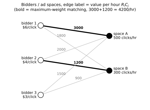
The bipartite graph of three advertisers and two ad spaces. Each edge is labelled with the value per hour \(v_{ij}=R_iC_j\); the two bold edges are the maximum-weight matching (bidder 1 to space A, bidder 2 to space B, total \$4200 per hour), and bidder 3 is left unmatched.
(b) The GSP outcome.
Truthful bidding is \(b = (6, 4, 3)\) per click. The GSP rule of Section 2.2.4 gives the \(i\)th most valuable space to the \(i\)th highest bidder at the \((i+1)\)th highest per-click bid, so space A goes to bidder 1 at \(b_2 = \$4\) per click (\(\$2000\) per hour), space B to bidder 2 at \(b_3 = \$3\) per click (\(\$900\) per hour), and bidder 3 gets and pays nothing. The allocation coincides with part (a)’s maximum matching, as it must for a rank-one valuation matrix under truthful bids. Payoffs are \(U_i = (R_i - p_i)C_j\).
b = R.copy()                        # truthful bidding: b_i = R_i
order = np.argsort(-b)              # bidders ranked by bid
for j, C_j in enumerate(C):         # space j (0=A, 1=B) to the (j+1)th highest bidder
    win, price = order[j], b[order[j+1]]
    print("space %s -> bidder %d | price %.2f/click | pays %.0f/hr | payoff %.0f/hr"
          % ("AB"[j], win+1, price, price*C_j, (R[win]-price)*C_j))
rev = sum(b[order[j+1]]*C[j] for j in range(len(C)))
pay = sum((R[order[j]]-b[order[j+1]])*C[j] for j in range(len(C)))
print("bidder 3: no space, price 0, payoff 0")
print("seller revenue %.0f/hr ; total bidder payoff %.0f/hr ; sum %.0f = matching weight"
      % (rev, pay, rev+pay))
space A -> bidder 1 | price 4.00/click | pays 2000/hr | payoff 1000/hr
space B -> bidder 2 | price 3.00/click | pays 900/hr | payoff 300/hr
bidder 3: no space, price 0, payoff 0
seller revenue 2900/hr ; total bidder payoff 1300/hr ; sum 4200 = matching weight
So bidder 1 nets \((6-4)\times 500 = \$1000\) per hour, bidder 2 nets \((4-3)\times 300 = \$300\), and bidder 3 nets \(0\); Google’s revenue \(\$2900\) plus the bidders’ \(\$1300\) recovers the matching weight \(\$4200\) per hour, as in Section 2.3.2.
Problem 2.2 — eBay Auction
eBay Auction. Alice lists a lamp for sale on eBay via auction with both the start price and reserve price set to $7.00 and a duration of 5 days. The minimal increment is $0.25 and the following events happen during the auction:
- Day 1: Bidder 1 uses a proxy agent, setting the maximum bid up to $11.00.
- Day 2: Bidder 2 bids $9.25.
- Day 3: Bidder 3 uses a proxy agent, setting the maximum bid up to $17.25.
- Day 4: Bidder 2 bids $13.65.
- Day 5: Bidder 1 bids $27.45.
List the bidding history of all three bidders over each day of the auction. Who is the winner and what price does she pay? (difficulty: \(\star\star\))
Bidder 1 wins the lamp and pays \(\$14.15\). Section 2.3.1 supplies the three rules, with \(\delta = \$0.25\): the displayed ask is \(\min\{b_1, b_2+\delta\} + \delta\) for current highest bid \(b_1\) and second highest \(b_2\); an outbid proxy agent reposts at whatever retakes the lead, and posts nothing at all once that exceeds its maximum (Table 2.1, where Alice’s \(\$12.00\) agent goes silent against Bob’s \(\$17.50\)); at hard close the winner pays \(\min\{b_1, b_2+\delta\}\). Start price and reserve coincide at \(\$7.00\), so the reserve binds only on the opening bid. Simulating the five days:
D = 25          # minimal increment, in cents
START = 700     # start price = reserve price

bid = {1: None, 2: None, 3: None}   # standing bid of each bidder, in cents
mx  = {}                            # proxy maxima, in cents
log = []

def high():
    live = [(v, i) for i, v in bid.items() if v is not None]
    if not live:
        return None, 0, None, 0
    live.sort(key=lambda t: -t[0])
    (b1, i1) = live[0]
    b2 = live[1][0] if len(live) > 1 else 0
    return i1, b1, (live[1][1] if len(live) > 1 else None), b2

def ask():
    i1, b1, i2, b2 = high()
    if i1 is None:
        return START
    return min(b1, b2 + D) + D if i2 is not None else b1 + D

def proxies():
    # a proxy raises to (current high bid + increment) whenever that is within its maximum
    moved = True
    while moved:
        moved = False
        i1, b1, _, _ = high()
        for i, m in mx.items():
            if i != i1 and b1 + D <= m:
                bid[i] = b1 + D
                log.append("    proxy %d -> %.2f" % (i, bid[i]/100))
                moved = True
                i1, b1, _, _ = high()

def day(n, msg):
    proxies()
    i1, b1, _, b2 = high()
    log.append("Day %d: %s | high = bidder %s at %.2f | ask = %.2f"
               % (n, msg, i1, b1/100, ask()/100))
    log.append("   standing bids: " + ", ".join(
        "b%d=%s" % (i, "-" if bid[i] is None else "%.2f" % (bid[i]/100)) for i in (1, 2, 3)))

# Day 1: bidder 1 enters a proxy with maximum 11.00; eBay bids the start price for her
mx[1] = 1100; bid[1] = START
day(1, "bidder 1 proxy (max 11.00) opens at the start price")

# Day 2: bidder 2 bids 9.25 by hand
bid[2] = 925
day(2, "bidder 2 bids 9.25")

# Day 3: bidder 3 enters a proxy with maximum 17.25, taking the current ask price
mx[3] = 1725; bid[3] = ask()
day(3, "bidder 3 proxy (max 17.25) takes the ask price")

# Day 4: bidder 2 bids 13.65 by hand
bid[2] = 1365
day(4, "bidder 2 bids 13.65")

# Day 5: bidder 1 bids 27.45 by hand, overriding her exhausted proxy
del mx[1]; bid[1] = 2745
day(5, "bidder 1 bids 27.45")

print("\n".join(log))
i1, b1, i2, b2 = high()
print("winner: bidder %d ; price = min(%.2f, %.2f + %.2f) = %.2f"
      % (i1, b1/100, b2/100, D/100, min(b1, b2 + D)/100))
Day 1: bidder 1 proxy (max 11.00) opens at the start price | high = bidder 1 at 7.00 | ask = 7.25
   standing bids: b1=7.00, b2=-, b3=-
    proxy 1 -> 9.50
Day 2: bidder 2 bids 9.25 | high = bidder 1 at 9.50 | ask = 9.75
   standing bids: b1=9.50, b2=9.25, b3=-
    proxy 1 -> 10.00
    proxy 3 -> 10.25
    proxy 1 -> 10.50
    proxy 3 -> 10.75
    proxy 1 -> 11.00
    proxy 3 -> 11.25
Day 3: bidder 3 proxy (max 17.25) takes the ask price | high = bidder 3 at 11.25 | ask = 11.50
   standing bids: b1=11.00, b2=9.25, b3=11.25
    proxy 3 -> 13.90
Day 4: bidder 2 bids 13.65 | high = bidder 3 at 13.90 | ask = 14.15
   standing bids: b1=11.00, b2=13.65, b3=13.90
Day 5: bidder 1 bids 27.45 | high = bidder 1 at 27.45 | ask = 14.40
   standing bids: b1=27.45, b2=13.65, b3=13.90
(Indented proxy lines are the automatic responses triggered within the day whose header follows.) Day by day:
- Day 1. Nobody has bid, so bidder 1’s agent opens at \(\$7.00\); ask \(\$7.25\).
- Day 2. Bidder 2’s \(\$9.25\) clears the ask, and bidder 1’s agent reposts at \(\$9.50\), inside her \(\$11.00\) maximum; ask \(\min\{9.50,\,9.50\}+0.25 = \$9.75\).
- Day 3. Two agents ratchet against each other in \(\$0.25\) steps — bidder 3 takes the \(\$9.75\) ask, bidder 1 answers \(\$10.00\), and so on — until bidder 1 posts her ceiling \(\$11.00\), bidder 3 answers \(\$11.25\), and bidder 1’s agent, needing \(\$11.50 > \$11.00\), stops; ask \(\min\{11.25,\,11.25\}+0.25 = \$11.50\).
- Day 4. Bidder 2 bids \(\$13.65\); bidder 1’s agent is exhausted and bidder 3’s answers \(\$13.90\), inside its \(\$17.25\) maximum; ask \(\min\{13.90,\,13.90\}+0.25 = \$14.15\).
- Day 5. Bidder 1 abandons her agent and bids \(\$27.45\) by hand. Bidder 3’s agent would need \(\$27.70 > \$17.25\), so it posts nothing; ask \(\min\{27.45,\,14.15\}+0.25 = \$14.40\).
The bidding history, in the format of Table 2.1:
| Bid | Day 1 | Day 2 | Day 3 | Day 4 | Day 5 |
|---|---|---|---|---|---|
| Bidder 1 | 7.00 | 9.50 | 11.00 | – | 27.45 |
| Bidder 2 | – | 9.25 | – | 13.65 | – |
| Bidder 3 | – | – | 11.25 | 13.90 | – |
| Ask price | 7.25 | 9.75 | 11.50 | 14.15 | 14.40 |
Nobody takes the \(\$14.40\) ask before the hard close, so bidder 1 wins with \(b_1 = \$27.45\) against bidder 3’s standing \(b_2 = \$13.90\) and pays \[ \min\{b_1,\, b_2 + \delta\} = \min\{27.45,\ 14.15\} = \$14.15 . \] This follows Table 2.1’s convention that a proxy which cannot retake the lead posts nothing; real eBay drives a losing agent to its maximum, so bidder 3 would post \(\$17.25\) and the price would be \(\$17.50\), with the same winner.
Problem 2.3 — More items than bidders
More items than bidders. Alice and Bob are bidding for three ad slots on a webpage, and one bidder can win at most one slot. Suppose the clickthrough rates are 500, 300, and 200 per hour, respectively. Assume that Alice receives $r per click.
(a) Denote by \(b_1\) and \(b_2\) the bids by Alice and Bob respectively. In GSP auction, discuss Alice’s payoff in terms of \(b_1\) and \(b_2\).
(b) Does Alice have a dominant strategy? If so, what is it? (difficulty: \(\star\))
(a) Alice’s payoff.
Write \(C_1 = 500\), \(C_2 = 300\), \(C_3 = 200\) clicks per hour and let \(p_{\min} \ge 0\) be the mandated minimum bid (Section 2.3.2; take \(p_{\min} = 0\)). With only two bidders slot 3 is never allocated. GSP gives the \(i\)th slot to the \(i\)th highest bidder at the \((i+1)\)th highest bid, so Alice pays Bob’s \(b_2\) when \(b_1 > b_2\), while if \(b_1 < b_2\) she takes slot 2 with no bid below her and pays only \(p_{\min}\): \[ U_1(b_1,b_2) \;=\; \begin{cases} C_1\,(r - b_2) \;=\; 500\,(r-b_2), & b_1 > b_2,\\[2pt] C_2\,(r - p_{\min}) \;=\; 300\,r, & b_1 < b_2 \quad (p_{\min}=0), \end{cases} \] averaged under whatever tie-break applies at \(b_1 = b_2\). Alice’s own bid appears in neither branch — it only selects the branch, the second-price decoupling of Section 2.2.3 — and losing the top slot still pays \(300r\), so winning it is better only when \[ 500\,(r-b_2) > 300\,r \iff 200\,r > 500\,b_2 \iff b_2 < \tfrac{2}{5}\,r = 0.4\,r . \]
(b) The dominant strategy.
Yes — the cutoff bid, which is not the truthful \(r\): \[ b_1^{*} \;=\; r - \frac{C_2}{C_1}\,\bigl(r - p_{\min}\bigr) \;=\; \frac{C_1 - C_2}{C_1}\,r + \frac{C_2}{C_1}\,p_{\min} \;=\; 0.4\,r \quad (p_{\min}=0). \] It is weakly dominant. If \(b_2 < 0.4r\) then \(b_1^{*} > b_2\) and Alice takes slot 1 for \(500(r-b_2) > 300r\); if \(b_2 > 0.4r\) then \(b_1^{*} < b_2\) and she takes slot 2 for \(300r > 500(r-b_2)\). Either way \(b_1^{*}\) attains the larger branch, and no other bid does so for every \(b_2\): any \(b_1 > 0.4r\) buys an overpriced top slot when \(b_2 \in (0.4r, b_1)\), and any \(b_1 < 0.4r\) forgoes a cheap one when \(b_2 \in (b_1, 0.4r)\). A grid search confirms uniqueness.
import numpy as np

C1, C2 = 500.0, 300.0
r = 10.0        # Alice's revenue per click
pmin = 0.0      # mandated minimum bid

def U(b1, b2):
    if b1 > b2:                      # Alice takes slot 1, pays Bob's bid
        return C1 * (r - b2)
    if b1 < b2:                      # Alice takes slot 2, pays the minimum bid
        return C2 * (r - pmin)
    return 0.5 * (C1 * (r - b2) + C2 * (r - pmin))

grid = np.round(np.arange(0.0, 12.001, 0.01), 2)     # candidate bids for both players
for b1 in grid:                       # is b1 a best reply to EVERY b2 ?
    if all(U(b1, b2) >= max(U(x, b2) for x in grid) - 1e-9 for b2 in grid):
        print("weakly dominant bid found: b1 = %.2f" % b1)
print("predicted cutoff r*(C1-C2)/C1 + pmin*C2/C1 = %.2f"
      % (r*(C1-C2)/C1 + pmin*C2/C1))
print("payoff at that bid, against b2 = 3.00 : %.0f ; against b2 = 6.00 : %.0f"
      % (U(4.0, 3.0), U(4.0, 6.0)))
print("truthful bid b1 = r = 10 against b2 = 6.00 : %.0f  (worse)" % U(10.0, 6.0))
weakly dominant bid found: b1 = 4.00
predicted cutoff r*(C1-C2)/C1 + pmin*C2/C1 = 4.00
payoff at that bid, against b2 = 3.00 : 3500 ; against b2 = 6.00 : 3000
truthful bid b1 = r = 10 against b2 = 6.00 : 2000  (worse)
Against Bob’s bid, the cutoff traces the upper envelope of every other strategy.
import matplotlib.pyplot as plt

def U(b1, b2):
    return C1*(r-b2) if b1 > b2 else C2*(r-pmin)

b2 = np.linspace(0, 10, 2001)
fig, ax = plt.subplots(figsize=(6.6, 4.0))
for b1, style, lab in [(10.0, "--", r"truthful, $b_1=r=10$"),
                       (4.0, "-", r"cutoff, $b_1=0.4r=4$"),
                       (2.0, ":", r"over-shaded, $b_1=2$")]:
    ax.plot(b2, [U(b1, x) for x in b2], style, lw=2.0, label=lab)
ax.axvline(4.0, color="0.6", lw=0.9)
ax.text(4.1, 4600, r"$b_2 = 0.4r$", fontsize=9, color="0.35")
ax.set_xlabel(r"Bob's bid $b_2$ (\$ per click)")
ax.set_ylabel(r"Alice's payoff (\$ per hour)")
ax.set_title("Alice's GSP payoff, 500/300/200 clicks per hour, $r=10$", fontsize=10)
ax.legend(fontsize=9, loc="upper right")
ax.grid(alpha=0.25)
plt.savefig('nl-ch02-gsp-cutoff-bid.svg', dpi=150, bbox_inches='tight')
print("wrote nl-ch02-gsp-cutoff-bid.svg")
wrote nl-ch02-gsp-cutoff-bid.svg
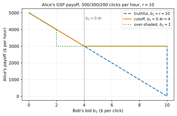
Alice’s GSP payoff as a function of Bob’s bid, for \(r=10\). Truthful bidding (\(b_1=10\)) drags her into overpriced top-slot wins whenever \(b_2 > 4\); over-shading (\(b_1=2\)) forfeits cheap top slots when \(2 < b_2 < 4\). The cutoff bid \(b_1 = 0.4r = 4\) is the upper envelope of both, for every value of \(b_2\).
This is the failure of truthfulness Section 2.3.3 draws from its 400/300 example: with \(C_1/C_2 = 5/3\) the gap in clickthrough rates is too small relative to the gap in per-click payment, and Alice shades to \(40\%\) of her true value because slot 2 is a free consolation prize.
Problem 2.4 — Reverse auction
Reverse auction. Reverse auction is a type of auction where there are multiple sellers and only one bidder. The roles of bidders and sellers are reversed, that is, sellers lower their bids during auction and the one with the lowest bid sells her item.
Suppose there are three sellers in a reverse auction with one bidder. Denote \(b_i\) as the price seller \(i\) bids, and \(v_i\) as the value seller \(i\) attaches to the item.
(a) In the case of second price auction, what is the payoff function for seller \(i\), as a function of \(b_1\), \(b_2\), and \(b_3\)?
(b) Is truthful bidding a dominant strategy? (difficulty: \(\star\))
(a) The payoff function.
Section 2.2.2 mirrored: the seller who asks least sells and is paid the second-lowest ask, giving up her own value \(v_i\), which plays the role the price played in the forward auction. Writing \[ m_i \;=\; \min_{j \neq i} b_j \] for the best competing ask, the payoff of seller \(i\) is \[ U_i(b_1,b_2,b_3) \;=\; \begin{cases} m_i - v_i, & b_i < m_i \quad \text{(she sells, and is paid } m_i),\\[2pt] 0, & b_i > m_i \quad \text{(she keeps her item)}. \end{cases} \] Spelled out, \(m_1 = \min\{b_2,b_3\}\), \(m_2 = \min\{b_1,b_3\}\), \(m_3 = \min\{b_1,b_2\}\); at a tie \(b_i = m_i\) the payoff is \(m_i - v_i\) with whatever probability the tie-break assigns.
(b) Truthful bidding is weakly dominant.
Yes. Fix the competitors’ asks, so \(m_i\) is outside seller \(i\)’s control; her bid decides only whether she sells, never the amount \(m_i\) she is paid, which is the decoupling of Section 2.2.3. Her attainable payoffs are thus \(m_i - v_i\) and \(0\), she wants to sell exactly when \(m_i > v_i\), and \(b_i = v_i\) implements that rule, attaining \(\max\{m_i - v_i,\, 0\}\) for every \(m_i\). The chapter’s two deviations, reversed:
- (i) \(\hat b_i > v_i\) changes the outcome only for \(m_i \in (v_i, \hat b_i)\), where she forgoes a sale worth \(m_i - v_i > 0\) and earns \(0\);
- (ii) \(\bar b_i < v_i\) changes it only for \(m_i \in (\bar b_i, v_i)\), where she sells at \(m_i - v_i < 0\) instead of earning \(0\).
Neither helps against any \((b_j)_{j \ne i}\), so \(b_i = v_i\) is weakly dominant. A grid check confirms it and exhibits both failure modes:
import numpy as np

def payoff(i, b, v):
    """reverse second price: lowest bidder sells and is paid the second-lowest bid"""
    m = min(b[j] for j in range(len(b)) if j != i)
    if b[i] < m:
        return m - v[i]
    if b[i] > m:
        return 0.0
    return 0.5 * (m - v[i])          # tie: coin flip between the two lowest

grid = np.round(np.arange(0.0, 10.01, 0.5), 2)
v1 = 4.0
worst_regret = 0.0
never_beaten = True
for b2 in grid:
    for b3 in grid:
        vals = {b1: payoff(0, [b1, b2, b3], [v1, 0, 0]) for b1 in grid}
        best = max(vals.values())
        regret = best - vals[v1]
        worst_regret = max(worst_regret, regret)
        if regret > 1e-9:
            never_beaten = False
print("v1 = %.1f ; over all (b2,b3) on the grid:" % v1)
print("worst-case shortfall of truthful bidding vs the best reply: %.10f" % worst_regret)
print("truthful bidding is a best reply to every (b2,b3):", never_beaten)

# the two deviations that the chapter's argument rules out
for b1, tag in [(6.0, "overbid b1=6 > v1"), (2.0, "underbid b1=2 < v1")]:
    for (b2, b3) in [(5.0, 9.0), (3.0, 9.0)]:
        print("%-22s vs (b2,b3)=(%.0f,%.0f): U=%.1f   truthful U=%.1f"
              % (tag, b2, b3, payoff(0, [b1, b2, b3], [v1, 0, 0]),
                 payoff(0, [v1, b2, b3], [v1, 0, 0])))
v1 = 4.0 ; over all (b2,b3) on the grid:
worst-case shortfall of truthful bidding vs the best reply: 0.0000000000
truthful bidding is a best reply to every (b2,b3): True
overbid b1=6 > v1      vs (b2,b3)=(5,9): U=0.0   truthful U=1.0
overbid b1=6 > v1      vs (b2,b3)=(3,9): U=0.0   truthful U=0.0
underbid b1=2 < v1     vs (b2,b3)=(5,9): U=1.0   truthful U=1.0
underbid b1=2 < v1     vs (b2,b3)=(3,9): U=-1.0   truthful U=0.0
The last line is case (ii): asking \(2\) for an item worth \(4\), against competitors at \(3\) and \(9\), buys a sale you did not want at a cost of \(1\).
Problem 2.5 — Spectrum auction and package bidding
Spectrum auction and package bidding. Wireless cellular technologies rely on spectrum assets. Around the world, auctions have emerged as the primary means of assigning spectrum licenses to companies wishing to provide wireless communication services. For example, from July 1994 to July 2011, the US Federal Communications Commission (FCC) conducted 92 spectrum auctions, raising over $60 billion for the US Treasury, and assigned thousands of licenses to hundreds of firms to different parts of the spectrum and different geographic regions of the country.
The US FCC uses simultaneous ascending auction, in which groups of related licenses are auctioned simultaneously and the winner pays the highest bid. The British OfCom, in contrast, runs package bidding, where each potential spectrum bidder can bid on a joint set of frequency bands.
Among the many issues involved in spectrum auctioning is the debate between simultaneous ascending auction and package bidding auction. We will illustrate the inefficiency resulting from disallowing package bidding in a toy example. The root cause for this inefficiency is “bidder-specific complementarity” and the lack of competition.
Suppose that there are two bidders for two adjacent seats in a movie theater. Bidder 1 is planning to watch the movie together with her spouse as part of a date. She values the two spots jointly at $15, and a single spot is worth nothing. Bidder 2 plans to watch the movie by himself, and values each seat at $10, and the two seats together at $12 (since it is a little nicer to have no one sitting next to him on one side of his seat).
(a) Assume a simultaneous ascending auction is used for the seats, and Bidder 1 correctly guesses that Bidder 2 values $10 for one seat and $12 for two seats together. What strategy will Bidder 1 take? What is the result of the auction, in terms of the allocation, the price charged, and the payoffs received?
(b) Repeat part (a) but now assume package bidding is used. In particular, Bidder 1 can bid on a package consisting of both seats. Explain the differences with (a). (difficulty: \(\star\star\))
Write the two seats as \(A\) and \(B\). The valuations are \[ v_1(\emptyset)=0,\quad v_1(A)=v_1(B)=0,\quad v_1(AB)=15, \] \[ v_2(\emptyset)=0,\quad v_2(A)=v_2(B)=10,\quad v_2(AB)=12. \] Bidder 1’s seats are perfect complements and bidder 2’s near-substitutes, his marginal value of a second seat being only \(v_2(AB) - v_2(A) = 2\). Total welfare is \(15\) for both seats to bidder 1, \(12\) for both to bidder 2, and \(10\) for one each, so the efficient allocation gives both to bidder 1.
(a) Simultaneous ascending auction: bidder 1 stays out, and bidder 2 takes both seats for nothing.
She must win both seats or neither. Were she to hold both at prices \(p_A, p_B\), bidder 2 — holding nothing, so valuing a first seat at \(10\) — must have found taking the cheaper one unprofitable: \[ \min\{p_A, p_B\} \;\ge\; 10 \quad\Longrightarrow\quad p_A + p_B \;\ge\; 20 \;>\; 15 = v_1(AB). \] Since he switches to whichever seat is cheaper, he forces both prices up to his single-seat value, and no price path leaves her holding the pair at a profit. Bidding naively to her full \(\$15\) is worse still: the auctions end with her paying for one worthless seat. That is the exposure problem, costing \(\$7.50\) below.
D = 0.5                       # bid increment; reserve price is 0

def price_to_take(p, who, s):
    return 0.0 if who[s] is None else p[s] + D     # free seat goes at the reserve

def saa(cap1):
    """simultaneous ascending auction on two seats.
       bidder 1 needs BOTH seats and will commit at most cap1 in total;
       bidder 2 pays up to 10 for a first seat and up to 12-10 = 2 for a second."""
    p = {"A": 0.0, "B": 0.0}
    who = {"A": None, "B": None}
    for _ in range(2000):
        acted = False
        held2 = [s for s in "AB" if who[s] == 2]
        free = sorted([s for s in "AB" if who[s] != 2], key=lambda s: p[s])
        if free:
            s = free[0]
            marginal = 10.0 if not held2 else 2.0
            if price_to_take(p, who, s) <= marginal:
                p[s] = price_to_take(p, who, s); who[s] = 2; acted = True
        need = [s for s in "AB" if who[s] != 1]
        if need:
            s = need[0]
            other = "B" if s == "A" else "A"
            bid = price_to_take(p, who, s)
            total = bid + (p[other] if who[other] == 1 else price_to_take(p, who, other))
            if total <= cap1:
                p[s] = bid; who[s] = 1; acted = True
        if not acted:
            break
    rev = sum(p.values())
    u1 = (15.0 if who["A"] == 1 and who["B"] == 1 else 0.0) \
         - sum(p[s] for s in "AB" if who[s] == 1)
    n2 = sum(1 for s in "AB" if who[s] == 2)
    u2 = {0: 0.0, 1: 10.0, 2: 12.0}[n2] - sum(p[s] for s in "AB" if who[s] == 2)
    return p, who, u1, u2, rev

for cap, tag in [(15.0, "bids up to her full value 15"), (0.0, "stays out of the auction")]:
    p, who, u1, u2, rev = saa(cap)
    print("bidder 1 %s:" % tag)
    print("   A -> %s at %.2f , B -> %s at %.2f" % (who["A"], p["A"], who["B"], p["B"]))
    print("   payoff 1 = %.2f , payoff 2 = %.2f , revenue = %.2f , welfare = %.2f"
          % (u1, u2, rev, u1 + u2 + rev))

print("what total outlay would she need to hold both seats?")
for cap in [15.0, 18.0, 20.0, 21.0]:
    p, who, *_ = saa(cap)
    print("   cap %5.1f -> wins both: %-5s (prices %.1f + %.1f)"
          % (cap, who["A"] == 1 and who["B"] == 1, p["A"], p["B"]))
bidder 1 bids up to her full value 15:
   A -> 2 at 8.00 , B -> 1 at 7.50
   payoff 1 = -7.50 , payoff 2 = 2.00 , revenue = 15.50 , welfare = 10.00
bidder 1 stays out of the auction:
   A -> 2 at 0.00 , B -> 2 at 0.00
   payoff 1 = 0.00 , payoff 2 = 12.00 , revenue = 0.00 , welfare = 12.00
what total outlay would she need to hold both seats?
   cap  15.0 -> wins both: False (prices 8.0 + 7.5)
   cap  18.0 -> wins both: False (prices 9.5 + 9.0)
   cap  20.0 -> wins both: False (prices 10.5 + 10.0)
   cap  21.0 -> wins both: True  (prices 10.5 + 10.5)
The last block makes the \(p_A + p_B \ge 20\) bound concrete: at a \(\$0.50\) increment she must be ready to spend \(\$21\) for a pair worth \(\$15\).
Guessing bidder 2’s values correctly, she runs this calculation first and stays out. Bidder 2 then faces no competition: he takes \(A\) at the reserve, and a second seat costing nothing while adding \(\$2\), he takes \(B\) too. Both seats therefore go to bidder 2 at effectively \(\$0\), with payoffs \(0\) to bidder 1 and \(\$12\) to bidder 2 and essentially no revenue — realized welfare \(\$12\) against the efficient \(\$15\), a deadweight loss of \(\$3\). The mechanism misallocates and raises nothing, the bidder who would have paid most having been driven out before it started.
(b) Package bidding: bidder 1 takes the pair at \(\$12\).
An all-or-nothing bid on \(\{A,B\}\) removes the exposure risk, so she can safely bid her full \(\$15\). Bidder 2’s best competing configuration is worth \(\max\{12,\ 10\} = 12\) — both seats at \(\$12\), or one at \(\$10\) with the other unsold and worthless to bidder 1 — so she raises her package bid until it clears \(\$12\) and he can no longer respond. The negative-externality charge of equation (2.1) gives the same number:
import itertools

v1 = {(): 0, ("A",): 0, ("B",): 0, ("A", "B"): 15}
v2 = {(): 0, ("A",): 10, ("B",): 10, ("A", "B"): 12}

def allocations():
    for assign in itertools.product([0, 1, 2], repeat=2):
        s1 = tuple(sorted(s for s, w in zip("AB", assign) if w == 1))
        s2 = tuple(sorted(s for s, w in zip("AB", assign) if w == 2))
        yield s1, s2

V = max(v1[s1] + v2[s2] for s1, s2 in allocations())            # efficient welfare
V_no1 = max(v2[s2] for s1, s2 in allocations() if s1 == ())     # welfare without bidder 1
V_no2 = max(v1[s1] for s1, s2 in allocations() if s2 == ())     # welfare without bidder 2
win = [(s1, s2) for s1, s2 in allocations() if v1[s1] + v2[s2] == V][0]
print("winning package allocation: bidder 1 gets %s, bidder 2 gets %s, welfare %d"
      % (win[0], win[1] or "()", V))
p1 = V_no1 - v2[win[1]]        # equation (2.1): damage bidder 1 does to the others
p2 = V_no2 - v1[win[0]]
print("VCG price for bidder 1 = %d - %d = %d" % (V_no1, v2[win[1]], p1))
print("VCG price for bidder 2 = %d - %d = %d" % (V_no2, v1[win[0]], p2))
print("payoffs: bidder 1 = %d, bidder 2 = %d ; seller revenue = %d" % (15 - p1, 0, p1))
winning package allocation: bidder 1 gets ('A', 'B'), bidder 2 gets (), welfare 15
VCG price for bidder 1 = 12 - 0 = 12
VCG price for bidder 2 = 15 - 15 = 0
payoffs: bidder 1 = 3, bidder 2 = 0 ; seller revenue = 12
Here \(p_1 = V_{\text{no }1} - \hat V_{1 \leftarrow AB} = 12 - 0 = 12\), so both seats go to bidder 1 — the efficient allocation — at \(\$12\), leaving her \(15 - 12 = \$3\), bidder 2 nothing, and the seller \(\$12\).
Differences with (a). Three, all in the same direction:
- Allocation. Welfare rises from \(\$12\) to \(\$15\); under (a) the seats went to the bidder who valued them less, purely because the format could not express “both or neither”.
- Revenue. The seller goes from roughly \(\$0\) to \(\$12\): forbidding package bids does not protect revenue but destroys it, by scaring off the highest-valuation bidder.
- Strategic burden. Under (a) bidder 1 must forecast her opponent’s whole valuation just to decide whether to enter, at a cost of \(\$7.50\) if she gets it wrong; under VCG package pricing the argument of Section 2.4.3 applies to packages, so bidding \(\$15\) truthfully is dominant.
How does Google rank webpages?
Problem 3.1 — PageRank sink
PageRank sink. Figure 3.5 shows a simple network of six webpages containing a sink node. The directed links are: \(1 \to 2\), \(2 \to 1\), \(2 \to 3\), \(1 \to 4\), \(4 \to 5\), \(5 \to 4\), \(5 \to 6\), and \(6 \to 4\). Node 3 has no outgoing link at all.
Write out the \(\mathbf{H}\) matrix of the graph in Figure 3.5. Iterate \(\pi[k]^T = \pi[k-1]^T \mathbf{H}\), where \(k = 0, 1, 2, \ldots\), and let the initialization be
\begin{equation*} \pi[0] = \begin{bmatrix} 1/6 & 1/6 & 1/6 & 1/6 & 1/6 & 1/6 \end{bmatrix}^T . \end{equation*}
What problem do you observe with the converged \(\pi^*\) vector? (difficulty: \(\star\))
The iteration converges to \(\pi^* = \begin{bmatrix}0&0&0&4/15&4/15&2/15\end{bmatrix}^T\), whose entries sum to \(2/3\) rather than \(1\): the sink destroys mass and the closed set \(\{4,5,6\}\) traps what is left. By Section 3.2.1, \(H_{ij} = 1/O_i\) on a link \(i \to j\) and \(0\) otherwise, with out-degrees \(O = (2,2,0,1,2,1)\), so
\begin{equation*} \mathbf{H} = \begin{bmatrix} 0 & 1/2 & 0 & 1/2 & 0 & 0\\ 1/2 & 0 & 1/2 & 0 & 0 & 0\\ 0 & 0 & 0 & 0 & 0 & 0\\ 0 & 0 & 0 & 0 & 1 & 0\\ 0 & 0 & 0 & 1/2 & 0 & 1/2\\ 0 & 0 & 0 & 1 & 0 & 0 \end{bmatrix}. \end{equation*}
Row 3 is all zeros — node 3 is the dangling node of Figure 3.2 — so \(\mathbf{H}\) is substochastic, the iteration is not a Markov chain, and whatever score sits on node 3 at step \(k\) vanishes at step \(k+1\). Meanwhile \(\{4,5,6\}\) is closed, while \(\{1,2\}\) is not: \(1 \to 4\) leaks into that closed set and \(2 \to 3\) into the sink. Writing \(s[k] = \pi_1[k] + \pi_2[k]\), nodes 1 and 2 each pass half their score to the other, so
\begin{equation*} s[k+1] = \tfrac{1}{2}s[k], \qquad s[0] = \tfrac{1}{3}, \end{equation*}
so pages 1, 2 and 3 decay geometrically to zero. The mass rescued from \(\{1,2\}\) is the flow \(\pi_1[k]/2\) summed across the link \(1 \to 4\):
\begin{equation*} \sum_{k \ge 0} \tfrac{1}{2}\pi_1[k] = \tfrac{1}{2}\sum_{k\ge 0} \tfrac{1}{6}\left(\tfrac{1}{2}\right)^{k} = \tfrac{1}{6}, \end{equation*}
the other \(1/6\) being swallowed by node 3, so with the \(1/2\) already inside \(\{4,5,6\}\) the surviving total is \(2/3\). Restricted to \(\{4,5,6\}\) the chain is irreducible and aperiodic (cycles \(4\to5\to4\) and \(4\to5\to6\to4\) give \(\gcd(2,3)=1\)), and its stationary vector solves \(x_4 = \tfrac12 x_5 + x_6\), \(x_5 = x_4\), \(x_6 = \tfrac12 x_5\), i.e. \((0.4,0.4,0.2)\) normalized. Scaling by \(2/3\),
\begin{equation*} \pi^* = \begin{bmatrix} 0 & 0 & 0 & 4/15 & 4/15 & 2/15 \end{bmatrix}^T . \end{equation*}
import numpy as np
np.set_printoptions(precision=6, suppress=True)

H = np.zeros((6, 6))
H[0, 1] = H[0, 3] = 0.5      # 1 -> 2, 1 -> 4
H[1, 0] = H[1, 2] = 0.5      # 2 -> 1, 2 -> 3
                             # row 3 stays all zeros: the sink
H[3, 4] = 1.0                # 4 -> 5
H[4, 3] = H[4, 5] = 0.5      # 5 -> 4, 5 -> 6
H[5, 3] = 1.0                # 6 -> 4

pi = np.ones(6) / 6
for k in range(1, 7):
    pi = pi @ H
    print(k, np.round(pi, 6), 'total', round(pi.sum(), 6))
for k in range(200):
    pi = pi @ H
print('k=206', np.round(pi, 6), 'total', round(pi.sum(), 6))
print('4/15, 2/15 =', round(4/15, 6), round(2/15, 6))
1 [0.083333 0.083333 0.083333 0.333333 0.166667 0.083333] total 0.833333
2 [0.041667 0.041667 0.041667 0.208333 0.333333 0.083333] total 0.75
3 [0.020833 0.020833 0.020833 0.270833 0.208333 0.166667] total 0.708333
4 [0.010417 0.010417 0.010417 0.28125  0.270833 0.104167] total 0.6875
5 [0.005208 0.005208 0.005208 0.244792 0.28125  0.135417] total 0.677083
6 [0.002604 0.002604 0.002604 0.278646 0.244792 0.140625] total 0.671875
k=206 [0.       0.       0.       0.266667 0.266667 0.133333] total 0.666667
4/15, 2/15 = 0.266667 0.133333
So the single zero row costs three things. (i) \(\pi^*\) is not a probability vector: its entries sum to \(2/3\) and the deficit depends on the initialization, so the normalization \(\sum_i \pi_i = 1\) of Section 3.2 fails and the scores are incomparable across graphs. (ii) Pages 1, 2 and 3 all score exactly zero and cannot be ranked against each other, even though node 3 is linked from node 2. (iii) All surviving score is trapped in the closed set \(\{4,5,6\}\), so any cluster linking only among itself absorbs the whole ranking budget — the structural germ of the SEO manipulation of Section 3.4.4. Section 3.2.2 patches the leak with \(\hat{\mathbf{H}} = \mathbf{H} + \frac{1}{N}\mathbf{w}\mathbf{1}^T\), \(\mathbf{w} = \begin{bmatrix}0&0&1&0&0&0\end{bmatrix}^T\), and equation (3.2)’s randomization breaks the trap.
Problem 3.2 — Cyclic ranking
Cyclic ranking. Figure 3.6 shows a simple network of four webpages arranged in a directed cycle: the only links are \(1 \to 2\), \(2 \to 3\), \(3 \to 4\), and \(4 \to 1\).
Write out the \(\mathbf{H}\) matrix of the graph in Figure 3.6. Iterate \(\pi[k]^T = \pi[k-1]^T \mathbf{H}\), where \(k = 0, 1, 2, \ldots\), and let the initialization be
\begin{equation*} \pi[0] = \begin{bmatrix} 1/2 & 1/2 & 0 & 0 \end{bmatrix}^T . \end{equation*}
What happens to the vectors \(\{\pi[k]\}\) as \(k\) becomes large? Solve for \(\pi^*\) such that \(\pi^{*T} = \pi^{*T}\mathbf{H}\) and \(\sum_i \pi_i^* = 1\). (difficulty: \(\star\))
The iterates never converge — they cycle with period 4 — while the fixed point is the uniform \(\pi^* = \begin{bmatrix}1/4&1/4&1/4&1/4\end{bmatrix}^T\). Every node has exactly one outgoing link, so \(O_i = 1\) and \(\mathbf{H}\) is the cyclic permutation matrix
\begin{equation*} \mathbf{H} = \begin{bmatrix} 0 & 1 & 0 & 0\\ 0 & 0 & 1 & 0\\ 0 & 0 & 0 & 1\\ 1 & 0 & 0 & 0 \end{bmatrix}. \end{equation*}
No node dangles, so \(\hat{\mathbf{H}} = \mathbf{H}\); every row sums to 1 and \(\mathbf{1}^T\pi[k] = 1\) for all \(k\), so unlike Problem 3.1 nothing leaks. Right-multiplication by \(\mathbf{H}\) shifts the score on node \(i\) to node \(i+1 \pmod 4\), so
\begin{equation*} \pi[k] = \mathbf{H}^{Tk}\pi[0], \qquad \mathbf{H}^4 = \mathbf{I}, \end{equation*}
and the sequence is exactly periodic with period 4:
\begin{equation*} \begin{bmatrix}\tfrac12\\tfrac12\\0\\0\end{bmatrix} \to \begin{bmatrix}0\\tfrac12\\tfrac12\\0\end{bmatrix} \to \begin{bmatrix}0\\0\\tfrac12\\tfrac12\end{bmatrix} \to \begin{bmatrix}\tfrac12\\0\\0\\tfrac12\end{bmatrix} \to \begin{bmatrix}\tfrac12\\tfrac12\\0\\0\end{bmatrix} \to \cdots \end{equation*}
No \(K\) has \(\pi[k] \approx \pi[k-1]\) for all \(k \ge K\): the power method (3.1) cycles forever through four distinct vectors, two of the four pages scoring zero at every step. Which two depends only on \(k \bmod 4\), so a ranking read off at iteration \(k\) is an artifact of when you stopped.
import numpy as np
np.set_printoptions(precision=4, suppress=True)

H = np.zeros((4, 4))
H[0, 1] = H[1, 2] = H[2, 3] = H[3, 0] = 1.0   # 1->2->3->4->1

pi = np.array([0.5, 0.5, 0.0, 0.0])
for k in range(1, 10):
    pi = pi @ H
    print('k =', k, pi)

ev = np.linalg.eigvals(H)
print('eigenvalues of H:', np.round(np.sort_complex(ev), 4))
print('Cesaro average of pi[1..400]:', np.round(
    np.mean([np.array([0.5,0.5,0,0]) @ np.linalg.matrix_power(H, k)
             for k in range(1, 401)], axis=0), 4))
k = 1 [0.  0.5 0.5 0. ]
k = 2 [0.  0.  0.5 0.5]
k = 3 [0.5 0.  0.  0.5]
k = 4 [0.5 0.5 0.  0. ]
k = 5 [0.  0.5 0.5 0. ]
k = 6 [0.  0.  0.5 0.5]
k = 7 [0.5 0.  0.  0.5]
k = 8 [0.5 0.5 0.  0. ]
k = 9 [0.  0.5 0.5 0. ]
eigenvalues of H: [-1.+0.j  0.-1.j  0.+1.j  1.+0.j]
Cesaro average of pi[1..400]: [0.25 0.25 0.25 0.25]
The spectrum \(\{1, i, -1, -i\}\) is the cause: four eigenvalues of modulus 1, the chain being periodic with period \(\gcd = 4\), so \(|\lambda_2| = 1\) and the contraction Section 3.4.1 relies on is absent. This is not the non-uniqueness Section 3.2.3 objects to in Figure 3.3 — here the eigenvalue 1 is simple, so the consistent score vector is unique and only the iteration fails, orbiting the fixed point without approaching it.
Reading \(\pi^{*T} = \pi^{*T}\mathbf{H}\) column by column,
\begin{equation*} \pi_1^* = \pi_4^*, \qquad \pi_2^* = \pi_1^*, \qquad \pi_3^* = \pi_2^*, \qquad \pi_4^* = \pi_3^*, \end{equation*}
so all four scores are equal and \(\sum_i \pi_i^* = 1\) pins them down:
\begin{equation*} \pi^* = \begin{bmatrix} 1/4 & 1/4 & 1/4 & 1/4 \end{bmatrix}^T . \end{equation*}
Periodicity destroys convergence of \(\pi[k]\) but not of its time average, and the Cesaro average of the iterates does converge to \(\pi^*\), as the last printed line shows.
Problem 3.3 — PageRank with different \(\theta\)
PageRank with different \(\theta\). Figure 3.7 shows a five-node web graph whose directed links are: \(1 \to 2\), \(2 \to 1\), \(3 \to 1\), \(3 \to 3\) (a self-loop), \(3 \to 5\), \(4 \to 3\), and \(4 \to 5\). Node 5 has no outgoing link, and node 4 has no incoming link.
Compute the PageRank vector \(\pi^*\) of the graph in Figure 3.7, for \(\theta = 0.1, 0.3, 0.5\), and \(0.85\). What do you observe? (difficulty: \(\star\star\))
The ranking is \(1 \succ 2 \succ (3 = 5) \succ 4\) at all four values of \(\theta\); what \(\theta\) changes is the spread of the scores and the cost of computing them. Out-degrees \(O = (1,1,3,2,0)\) give
\begin{equation*} \mathbf{H} = \begin{bmatrix} 0 & 1 & 0 & 0 & 0\\ 1 & 0 & 0 & 0 & 0\\ 1/3 & 0 & 1/3 & 0 & 1/3\\ 0 & 0 & 1/2 & 0 & 1/2\\ 0 & 0 & 0 & 0 & 0 \end{bmatrix}. \end{equation*}
Node 5 is dangling, so \(\mathbf{w} = \begin{bmatrix}0&0&0&0&1\end{bmatrix}^T\) and Section 3.2.2 gives \(\hat{\mathbf{H}} = \mathbf{H} + \frac{1}{5}\mathbf{w}\mathbf{1}^T\), i.e. row 5 becomes \(\begin{bmatrix}1/5&1/5&1/5&1/5&1/5\end{bmatrix}\). Then equation (3.2) gives \(\mathbf{G} = \theta\hat{\mathbf{H}} + (1-\theta)\frac{1}{5}\mathbf{1}\mathbf{1}^T\) and \(\pi^*\) is the dominant left eigenvector (3.4).
Three structural facts fix the shape of the answer. (i) Nodes 3 and 5 draw on identical sources under \(\hat{\mathbf{H}}\) — each takes \(\theta\pi_3/3\) from node 3, \(\theta\pi_4/2\) from node 4 and \(\theta\pi_5/5\) from the dangling row, with equal teleport — so \(\pi_3^* = \pi_5^*\) identically in \(\theta\), a permanent tie. (ii) Node 4 has in-degree zero in \(\mathbf{H}\), so its only income is the dangling row and the teleport,
\begin{equation*} \pi_4^* = \frac{\theta}{5}\pi_5^* + \frac{1-\theta}{5}, \end{equation*}
and it ranks last for every \(\theta\), with \(\pi_4^* \to 0\) as \(\theta \to 1\). (iii) The pair \(\{1,2\}\) is closed under \(\mathbf{H}\), fed only by \(3 \to 1\) and the dangling row and drained only by teleport, so \(\pi_1^* + \pi_2^* \to 1\) as \(\theta \to 1\) — the trap of Problem 3.1 again.
import numpy as np
np.set_printoptions(precision=4, suppress=True)

N = 5
H = np.zeros((N, N))
H[0, 1] = 1.0                          # 1 -> 2
H[1, 0] = 1.0                          # 2 -> 1
H[2, 0] = H[2, 2] = H[2, 4] = 1/3      # 3 -> 1, 3 -> 3, 3 -> 5
H[3, 2] = H[3, 4] = 0.5                # 4 -> 3, 4 -> 5
                                       # row 5 is zero: node 5 is dangling
w = (H.sum(axis=1) == 0).astype(float)
Hhat = H + np.outer(w, np.ones(N)) / N
print('H =\n', H)
print('w =', w)

def pagerank(theta, tol=1e-12):
    G = theta * Hhat + (1 - theta) * np.ones((N, N)) / N
    pi = np.ones(N) / N
    k = 0
    while True:
        k += 1
        nxt = pi @ G
        if np.abs(nxt - pi).max() < tol:
            return nxt / nxt.sum(), k
        pi = nxt

for theta in [0.1, 0.3, 0.5, 0.85]:
    pi, k = pagerank(theta)
    order = list(np.argsort(-pi) + 1)
    print('theta = %.2f  pi* = %s  ranking %s  (%3d iterations)'
          % (theta, np.round(pi, 4), order, k))
H =
 [[0.     1.     0.     0.     0.    ]
 [1.     0.     0.     0.     0.    ]
 [0.3333 0.     0.3333 0.     0.3333]
 [0.     0.     0.5    0.     0.5   ]
 [0.     0.     0.     0.     0.    ]]
w = [0. 0. 0. 0. 1.]
theta = 0.10  pi* = [0.2112 0.2051 0.1999 0.184  0.1999]  ranking [1, 2, 3, 5, 4]  ( 11 iterations)
theta = 0.30  pi* = [0.2379 0.223  0.1937 0.1516 0.1937]  ranking [1, 2, 3, 5, 4]  ( 20 iterations)
theta = 0.50  pi* = [0.2745 0.2549 0.1765 0.1176 0.1765]  ranking [1, 2, 3, 5, 4]  ( 35 iterations)
theta = 0.85  pi* = [0.3941 0.3803 0.0901 0.0453 0.0901]  ranking [1, 2, 3, 5, 4]  (147 iterations)
The printed ranking puts 3 before 5 only because argsort has to break the exact tie somehow; the true ordering is \(1 \succ 2 \succ (3 = 5) \succ 4\).
import numpy as np
import matplotlib
matplotlib.use('Agg')
import matplotlib.pyplot as plt

N = 5
H = np.zeros((N, N))
H[0,1]=1.0; H[1,0]=1.0
H[2,0]=H[2,2]=H[2,4]=1/3
H[3,2]=H[3,4]=0.5
w = (H.sum(axis=1) == 0).astype(float)
Hhat = H + np.outer(w, np.ones(N)) / N

def exact_pr(theta):
    G = theta * Hhat + (1 - theta) * np.ones((N, N)) / N
    ev, V = np.linalg.eig(G.T)
    v = np.real(V[:, np.argmin(np.abs(ev - 1))])
    return v / v.sum()

th = np.linspace(0.0, 0.995, 300)
P = np.array([exact_pr(t) for t in th])

plt.figure(figsize=(7, 4.2))
styles = ['-', '-', '-', '-', '--']     # node 5 dashed: it sits exactly on node 3
for i in range(N):
    plt.plot(th, P[:, i], lw=2, ls=styles[i], label='node %d' % (i + 1))
for t in [0.1, 0.3, 0.5, 0.85]:
    plt.axvline(t, color='gray', ls='--', lw=0.7)
plt.axhline(0.2, color='gray', ls=':', lw=1)
plt.xlabel(r'$\theta$'); plt.ylabel(r'$\pi^*_i$')
plt.title(r'PageRank of Figure 3.7 as a function of $\theta$')
plt.legend(ncol=5, fontsize=8); plt.grid(alpha=0.25)
plt.savefig('nl-ch03-pagerank-vs-theta.svg', dpi=150, bbox_inches='tight')

print('theta = 0.995 :', np.round(P[-1], 4))
print('pi_1 + pi_2 at theta = 0.995 :', round(P[-1][:2].sum(), 4))
print('max |pi_3 - pi_5| over the sweep :', np.abs(P[:,2]-P[:,4]).max())
theta = 0.995 : [0.4954 0.4947 0.004  0.0018 0.004 ]
pi_1 + pi_2 at theta = 0.995 : 0.9901
max |pi_3 - pi_5| over the sweep : 1.942890293094024e-16
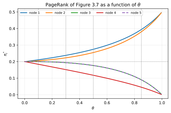
PageRank scores of the five webpages of Figure 3.7 as \(\theta\) is swept from 0 to 1. All curves leave the uniform value \(1/5\) at \(\theta = 0\) and fan out without ever crossing; nodes 3 and 5 coincide exactly (node 5 is dashed on top of node 3), and the closed pair \(\{1,2\}\) absorbs essentially all the score as \(\theta \to 1\). The dashed verticals mark \(\theta = 0.1, 0.3, 0.5, 0.85\).
Four observations.
- The ranking is invariant: \(1 \succ 2 \succ (3 = 5) \succ 4\) at all four values, with no crossing anywhere in \(\theta \in [0,1)\). What \(\theta\) controls is the spread, not the order — which is what licenses Section 3.4.3 to relax the meaning of convergence.
- It interpolates between ignoring and trusting the graph. At \(\theta = 0\), \(\mathbf{G} = \frac{1}{5}\mathbf{1}\mathbf{1}^T\) and \(\pi^*\) is uniform; the scores span \([0.184, 0.211]\) at \(\theta = 0.1\) but \([0.045, 0.394]\) at \(\theta = 0.85\), with \(\pi_1^*/\pi_4^*\) running \(1.15, 1.57, 2.33, 8.70\).
- Convergence costs \(11, 20, 35, 147\) iterations at tolerance \(10^{-12}\). Since \(\lambda_2(\mathbf{G}) \approx \theta\) (Section 3.4.1), the error contracts like \(\theta^k\) and the count should scale as \(\log(\text{tol})/\log\theta\), predicting \(12, 23, 40, 170\).
- As \(\theta \to 1\) the closed pair \(\{1,2\}\) swallows the budget: \(\pi_1^* + \pi_2^* = 0.99\) at \(\theta = 0.995\). That is the link-manipulation structure of Section 3.4.4 in miniature, and \((\mathbf{I}-\theta\mathbf{H})^{-1}\) in equation (3.6) blows up there too, so the scores swing hard on small changes in \(\theta\).
Problem 3.4 — Block aggregation in PageRank
Block aggregation in PageRank. Set \(\theta = 0.85\) and start with any normalized initial vector \(\pi[0]\).
Figure 3.8 shows two graphs that will be superimposed later. Figure 3.8(a) is a two-node graph on supernodes \(A\) and \(B\): \(A\) has a self-loop of weight 1, and \(B\) splits its weight \(1/3\) to \(A\) and \(2/3\) to its own self-loop. Figure 3.8(b) is a pair of separate graphs: on the left, nodes 1 and 2 with links \(1 \to 2\) and \(2 \to 1\); on the right, nodes 3, 4, 5 with links \(3 \to 3\) (a self-loop), \(3 \to 5\), \(4 \to 3\), and \(4 \to 5\), so that node 5 is dangling. Figure 3.9 shows the graph of Figure 3.7 with its nodes grouped into block \(A = \{1,2\}\) and block \(B = \{3,4,5\}\); the only link crossing between blocks is \(3 \to 1\).
(a) Compute the PageRank vector \(\begin{bmatrix}\pi_A^* & \pi_B^*\end{bmatrix}^T\) of the graph in Figure 3.8(a) with
\begin{equation*} \mathbf{H} = \begin{bmatrix} 1 & 0 \\ 1/3 & 2/3 \end{bmatrix}. \end{equation*}
Note the uneven splitting of link weights from node \(B\). This will be useful later in the problem.
(b) Compute the PageRank vectors \(\begin{bmatrix}\pi_1^* & \pi_2^*\end{bmatrix}^T\) and \(\begin{bmatrix}\pi_3^* & \pi_4^* & \pi_5^*\end{bmatrix}^T\) of the two graphs in Figure 3.8(b).
(c) If we divide the graph in Figure 3.7 into two blocks as shown in Figure 3.9, we can approximate \(\pi^*\) in the previous question by
\begin{equation*} \tilde{\pi}^* = \begin{bmatrix} \pi_A^*\cdot\begin{bmatrix}\pi_1^* & \pi_2^*\end{bmatrix} & \pi_B^*\cdot\begin{bmatrix}\pi_3^* & \pi_4^* & \pi_5^*\end{bmatrix}\end{bmatrix}^T . \end{equation*}
Compute this vector. Explain the advantage, in terms of computational load, of using this approximation instead of directly computing \(\pi^*\). (difficulty: \(\star\star\))
This is item 5 of Section 3.4.3: rank the clusters as if each were a single page, then split each cluster’s score among its members by the cluster’s own internal PageRank, so that two small eigenproblems replace one big one.
Part (a), the inter-block problem. Both rows of the given \(\mathbf{H}\) sum to 1, so \(\hat{\mathbf{H}} = \mathbf{H}\), and with \(N = 2\), \(\theta = 0.85\),
\begin{equation*} \mathbf{G} = 0.85\begin{bmatrix}1 & 0\\ 1/3 & 2/3\end{bmatrix} + 0.075\begin{bmatrix}1&1\\1&1\end{bmatrix} = \begin{bmatrix} 0.925 & 0.075 \\ 43/120 & 77/120\end{bmatrix}. \end{equation*}
Detailed balance across the single cut, \(\pi_A^* G_{AB} = \pi_B^* G_{BA}\), solves a two-state chain outright:
\begin{equation*} \frac{\pi_A^*}{\pi_B^*} = \frac{G_{BA}}{G_{AB}} = \frac{43/120}{9/120} = \frac{43}{9}, \qquad \begin{bmatrix}\pi_A^* \\ \pi_B^*\end{bmatrix} = \begin{bmatrix}43/52 \\ 9/52\end{bmatrix} = \begin{bmatrix}0.826923 \\ 0.173077\end{bmatrix}. \end{equation*}
The uneven splitting the problem points at gives \(A\) about 83 percent of the score: \(B\) leaks a third of its weight into \(A\) and \(A\) leaks nothing back, making \(A\) near-absorbing.
Part (b), the two intra-block problems. Subgraph \(A\) has \(\mathbf{H}_A = \begin{bmatrix}0&1\\1&0\end{bmatrix}\), symmetric under swapping its nodes, so \(\begin{bmatrix}\pi_1^* & \pi_2^*\end{bmatrix}^T = \begin{bmatrix}1/2 & 1/2\end{bmatrix}^T\). Subgraph \(B\) is taken in isolation, so the link \(3 \to 1\) is gone and \(O_3 = 2\):
\begin{equation*} \mathbf{H}_B = \begin{bmatrix} 1/2 & 0 & 1/2 \\ 1/2 & 0 & 1/2 \\ 0 & 0 & 0\end{bmatrix}, \qquad \hat{\mathbf{H}}_B = \begin{bmatrix} 1/2 & 0 & 1/2 \\ 1/2 & 0 & 1/2 \\ 1/3 & 1/3 & 1/3\end{bmatrix}, \end{equation*}
and, since \((1-\theta)/3 = 0.05\) and \(0.85/3 + 0.05 = 1/3\),
\begin{equation*} \mathbf{G}_B = \begin{bmatrix} 0.475 & 0.05 & 0.475 \\ 0.475 & 0.05 & 0.475 \\ 1/3 & 1/3 & 1/3 \end{bmatrix}. \end{equation*}
Columns 3 and 5 of \(\mathbf{G}_B\) are identical, both \(\begin{bmatrix}0.475 & 0.475 & 1/3\end{bmatrix}^T\), so \(\pi_3^* = \pi_5^*\) again. With \(s = \pi_3^* + \pi_4^*\), \(\pi_5^* = 0.475s + \pi_5^*/3\) gives \(\pi_5^* = \tfrac{57}{80}s\), and \(\pi_4^* = 0.05s + \pi_5^*/3 = \tfrac{23}{80}s\). Normalizing, \(s + \tfrac{57}{80}s = \tfrac{137}{80}s = 1\), so
\begin{equation*} \begin{bmatrix}\pi_3^* \\ \pi_4^* \\ \pi_5^*\end{bmatrix} = \begin{bmatrix}57/137 \\ 23/137 \\ 57/137\end{bmatrix} = \begin{bmatrix}0.416058 \\ 0.167883 \\ 0.416058\end{bmatrix}. \end{equation*}
Part (c), assembling.
\begin{equation*} \tilde{\pi}^* = \begin{bmatrix} \tfrac{43}{52}\cdot\tfrac12 & \tfrac{43}{52}\cdot\tfrac12 & \tfrac{9}{52}\cdot\tfrac{57}{137} & \tfrac{9}{52}\cdot\tfrac{23}{137} & \tfrac{9}{52}\cdot\tfrac{57}{137}\end{bmatrix}^T = \begin{bmatrix} \tfrac{43}{104} & \tfrac{43}{104} & \tfrac{513}{7124} & \tfrac{207}{7124} & \tfrac{513}{7124}\end{bmatrix}^T . \end{equation*}
import numpy as np
np.set_printoptions(precision=6, suppress=True)
theta = 0.85

def pagerank(H, tol=1e-14):
    N = H.shape[0]
    w = (H.sum(axis=1) == 0).astype(float)
    Hhat = H + np.outer(w, np.ones(N)) / N
    G = theta * Hhat + (1 - theta) * np.ones((N, N)) / N
    pi, k = np.ones(N) / N, 0
    while True:
        k += 1
        nxt = pi @ G
        if np.abs(nxt - pi).max() < tol:
            return nxt / nxt.sum(), k
        pi = nxt

# (a) the two-supernode graph of Figure 3.8(a)
H_AB = np.array([[1.0, 0.0],
                 [1/3, 2/3]])
piAB, kAB = pagerank(H_AB)
print('(a) [piA piB] =', np.round(piAB, 6), ' 43/52, 9/52 =',
      round(43/52, 6), round(9/52, 6), ' iters', kAB)

# (b) the two subgraphs of Figure 3.8(b), each ranked on its own
H_A = np.array([[0.0, 1.0],      # 1 -> 2
                [1.0, 0.0]])     # 2 -> 1
H_B = np.array([[0.5, 0.0, 0.5],  # 3 -> 3, 3 -> 5
                [0.5, 0.0, 0.5],  # 4 -> 3, 4 -> 5
                [0.0, 0.0, 0.0]]) # 5 dangling
piA, kA = pagerank(H_A)
piB, kB = pagerank(H_B)
print('(b) [pi1 pi2]      =', np.round(piA, 6), ' iters', kA)
print('(b) [pi3 pi4 pi5]  =', np.round(piB, 6),
      ' 57/137, 23/137 =', round(57/137, 6), round(23/137, 6), ' iters', kB)

# (c) hierarchical assembly, versus the direct answer of Problem 3.3
tilde = np.concatenate([piAB[0] * piA, piAB[1] * piB])
H5 = np.zeros((5, 5))
H5[0,1]=1.0; H5[1,0]=1.0
H5[2,0]=H5[2,2]=H5[2,4]=1/3
H5[3,2]=H5[3,4]=0.5
exact, k5 = pagerank(H5)
print('(c) tilde pi* =', np.round(tilde, 6), ' sum', round(tilde.sum(), 12))
print('(c) exact pi* =', np.round(exact, 6), ' iters', k5)
print('(c) abs error =', np.round(np.abs(tilde - exact), 6),
      ' max', round(np.abs(tilde - exact).max(), 6))
print('(c) ranking, approx', list(np.argsort(-tilde) + 1),
      ' exact', list(np.argsort(-exact) + 1))
(a) [piA piB] = [0.826923 0.173077]  43/52, 9/52 = 0.826923 0.173077  iters 55
(b) [pi1 pi2]      = [0.5 0.5]  iters 1
(b) [pi3 pi4 pi5]  = [0.416058 0.167883 0.416058]  57/137, 23/137 = 0.416058 0.167883  iters 17
(c) tilde pi* = [0.413462 0.413462 0.07201  0.029057 0.07201 ]  sum 1.0
(c) exact pi* = [0.39413  0.38033  0.090111 0.045319 0.090111]  iters 176
(c) abs error = [0.019331 0.033132 0.018101 0.016262 0.018101]  max 0.033132
(c) ranking, approx [1, 2, 3, 5, 4]  exact [1, 2, 3, 5, 4]
Being a product of probability vectors, \(\tilde{\pi}^*\) is automatically normalized, and it reproduces the exact ranking \(1 \succ 2 \succ (3 = 5) \succ 4\) of Problem 3.3 to a worst-case score error of \(0.033\). That error is largest on node 2, and for a reason: aggregation assumes score entering a block spreads by the block’s own internal stationary vector, whereas score enters \(A\) only through \(3 \to 1\), landing on node 1 and reaching node 2 a hop later. Hence the exact \(\pi_1^* > \pi_2^*\) (\(0.394\) against \(0.380\)) where symmetry of the isolated subgraph forces the approximation to tie them. Block aggregation is exact only for a lumpable chain — every node of a block having the same total transition probability into each other block — so the residual measures how far the partition is from lumpable.
Computational load. Directly, the power iteration on a dense \(5\times5\) \(\mathbf{G}\) is 25 multiplications per iteration over 176 iterations, about 4400. Hierarchically it is \(2\times2\) for the supernodes (55 iterations), \(2\times2\) for block \(A\) (1), \(3\times3\) for block \(B\) (17), plus five products to assemble: \(55\cdot4 + 1\cdot4 + 17\cdot9 + 5 = 382\). The scaling argument is what carries: partition \(N\) pages into \(m\) blocks of \(N/m\). A direct iteration costs \(O(N^2)\); a hierarchical one costs \(m(N/m)^2 = N^2/m\) across all intra-block problems plus \(m^2\) for the inter-block problem, so
\begin{equation*} \text{cost per iteration}: \quad N^2 \;\longrightarrow\; \frac{N^2}{m} + m^2 , \end{equation*}
minimized near \(m = (N^2/2)^{1/3}\), giving \(O(N^{4/3})\) in place of \(O(N^2)\). At web scale three further gains matter as much: the \(m\) intra-block problems are independent and parallelize with no communication, a changed link inside one block forces only that block to be recomputed, and the scheme recurses into sub-blocks for the same saving at each level.
Problem 3.5 — Personalized ranking (open-ended)
Personalized ranking. How would you solicit and aggregate feedback from individual users to enable personalized ranking? (open-ended)
Solicit feedback implicitly from click and dwell logs, aggregate it into a low-dimensional topic profile rather than into per-user link weights, and inject it as the teleport vector \(\mathbf{v}\) of the generalized PageRank equation (3.5): because \(\pi^*\) is exactly linear in \(\mathbf{v}\), a personalized ranking is then a convex combination of a handful of precomputed vectors, one dot product per query instead of one eigenproblem per user.
Equation (3.5) exposes three tunable objects,
\begin{equation*} \pi^T\mathbf{G} = \theta\pi^T\mathbf{H} + \pi^T\big(\theta\mathbf{w} + (1-\theta)\mathbf{1}\big)\mathbf{v}^T , \end{equation*}
and only \(\mathbf{v}\) is cheap. Reweighting each user’s hyperlink graph by their click frequencies — what Section 3.4.3 proposes as a global correction — is ruinous per user: a per-user \(\mathbf{H}\) means a per-user dominant-eigenvector computation over billions of pages and a per-user copy of a matrix as sparse as the whole web. Personalizing \(\theta\) achieves nothing, since Problem 3.3 showed the ranking invariant across its whole range.
Take a web with no dangling nodes, \(\mathbf{w} = \mathbf{0}\). Since \(\pi^T\mathbf{1} = 1\), the fixed point of (3.5) satisfies
\begin{equation*} \pi^T(\mathbf{I} - \theta\mathbf{H}) = (1-\theta)\mathbf{v}^T, \qquad\text{i.e.}\qquad \pi = (1-\theta)\big[(\mathbf{I} - \theta\mathbf{H})^T\big]^{-1}\mathbf{v}, \end{equation*}
which is the chapter’s equation (3.6), \((\mathbf{I} - \theta\mathbf{H})^T\pi = \mathbf{v}\), up to the scalar \((1-\theta)\) that the book absorbs by leaving its \(\pi\) unnormalized (its derivation assumes only \(\mathbf{1}^T\mathbf{v} = 1\), so with \(\mathbf{w} = \mathbf{0}\) its solution has \(\mathbf{1}^T\pi = 1/(1-\theta)\) and is rescaled before ranking). So \(\mathbf{v} \mapsto \pi^*(\mathbf{v})\) is a fixed linear operator: if \(\mathbf{v} = \sum_c \alpha_c \mathbf{v}_c\) with \(\alpha\) on the simplex, then \(\pi^*(\mathbf{v}) = \sum_c \alpha_c\,\pi^*(\mathbf{v}_c)\) exactly. Precompute \(\pi^*(\mathbf{v}_c)\) offline for \(C\) topic basis vectors by the ordinary power method; storage is \(C\) vectors rather than one per user, and query-time work is \(O(CN)\) with no iteration.
The scheme has three steps. (i) Solicit implicitly, since explicit ratings are sparse, biased and gameable: use the click stream gated on dwell time, so a click followed by an immediate back-button counts negative, with a correction for position bias. (ii) Aggregate into a profile rather than a vector over pages — one user’s clicks touch a vanishing fraction of \(N\), so a raw per-page teleport vector is overfitted — by mapping each clicked page to its topic, accumulating counts \(n_c\), and shrinking toward the population prior with a Dirichlet pseudo-count \(\kappa\):
\begin{equation*} \alpha_c = \frac{n_c + \kappa/C}{\sum_{c^{\prime}} n_{c^{\prime}} + \kappa}. \end{equation*}
With no history \(\alpha\) is uniform and the user gets the global PageRank, so a new user degrades gracefully; the shrinkage is also the manipulation defense Section 3.4.4 would want, since a few injected clicks cannot move \(\alpha\) far and even a captured \(\alpha\) reshapes only that user’s ranking, unlike link spam against \(\mathbf{H}\). (iii) Serve \(\pi^*_{\text{user}} = \sum_c \alpha_c \pi^*(\mathbf{v}_c)\), combined with the relevance score as in Section 3.2.
Two claims carry the argument — that the linearity is exact, and that a realistic click log moves the ranking enough to matter:
import numpy as np
np.set_printoptions(precision=3, suppress=True)
rng = np.random.default_rng(11)

# --- a toy web: 3 topical clusters of 10 pages, dense inside, sparse across
N, C, sz = 30, 3, 10
topic = np.repeat(np.arange(C), sz)
A = np.zeros((N, N), dtype=int)
for i in range(N):
    for j in range(N):
        if i != j:
            A[i, j] = rng.random() < (0.25 if topic[i] == topic[j] else 0.012)
for i in range(N):                        # keep the toy web free of dangling nodes
    if A[i].sum() == 0:
        A[i, (i + 1) % N] = 1
H = A / A.sum(axis=1, keepdims=True)
intra = sum(A[i, j] for i in range(N) for j in range(N) if topic[i] == topic[j])
inter = A.sum() - intra
print('links: intra =', int(intra), ' inter =', int(inter))

theta = 0.85
def pagerank_v(v, tol=1e-15):
    G = theta * H + (1 - theta) * np.outer(np.ones(N), v)
    pi = np.ones(N) / N
    for _ in range(200000):
        nxt = pi @ G
        if np.abs(nxt - pi).max() < tol:
            return nxt / nxt.sum()
        pi = nxt

basis = np.array([(topic == c) / sz for c in range(C)])   # one teleport per topic
PI = np.array([pagerank_v(b) for b in basis])
pi_global = pagerank_v(np.ones(N) / N)

alpha = np.array([0.6, 0.3, 0.1])
print('linearity, max |pi(mix) - mix of pi| =',
      np.abs(pagerank_v(alpha @ basis) - alpha @ PI).max())

def profile(clicks, kappa=3.0):
    counts = np.array([clicks[topic == c].sum() for c in range(C)])
    return (counts + kappa / C) / (counts.sum() + kappa)   # Dirichlet shrinkage

clicks = {'ann': np.zeros(N), 'bo': np.zeros(N)}
clicks['ann'][[1, 3, 4, 7, 9, 22]] = [4, 2, 3, 1, 2, 1]
clicks['bo'][[21, 23, 24, 28, 12]] = [5, 3, 2, 2, 1]
top = lambda p, k=6: [int(i) + 1 for i in np.argsort(-p)[:k]]
print('cluster of pages 1-10 = topic 1, 11-20 = topic 2, 21-30 = topic 3')
print('%-6s %-21s %s' % ('who', 'alpha', 'top-6 pages'))
print('%-6s %-21s %s' % ('global', str(np.round(np.ones(3)/3, 3)), top(pi_global)))
P = {}
for u in clicks:
    a = profile(clicks[u]); P[u] = a @ PI
    print('%-6s %-21s %s' % (u, str(np.round(a, 3)), top(P[u])))

def kendall(x, y):
    n = len(x)
    s = sum(np.sign(x[i]-x[j]) * np.sign(y[i]-y[j])
            for i in range(n) for j in range(i+1, n))
    return 2 * s / (n * (n - 1))
print('Kendall tau  ann vs global = %.3f' % kendall(P['ann'], pi_global))
print('Kendall tau  bo  vs global = %.3f' % kendall(P['bo'],  pi_global))
print('Kendall tau  ann vs bo     = %.3f' % kendall(P['ann'], P['bo']))
print('top-6 overlap ann/bo =', len(set(top(P['ann'])) & set(top(P['bo']))))
print('global score mass per topic =',
      np.round([pi_global[topic == c].sum() for c in range(C)], 4))
links: intra = 78  inter = 6
linearity, max |pi(mix) - mix of pi| = 1.5404344466674047e-15
cluster of pages 1-10 = topic 1, 11-20 = topic 2, 21-30 = topic 3
who    alpha                 top-6 pages
global [0.333 0.333 0.333]   [22, 24, 8, 14, 15, 25]
ann    [0.812 0.062 0.125]   [8, 5, 4, 3, 10, 2]
bo     [0.062 0.125 0.812]   [24, 22, 25, 29, 21, 8]
Kendall tau  ann vs global = 0.469
Kendall tau  bo  vs global = 0.506
Kendall tau  ann vs bo     = 0.069
top-6 overlap ann/bo = 1
global score mass per topic = [0.342 0.337 0.322]
The linearity residual is \(1.5\times10^{-15}\), machine precision, so recombining the precomputed basis vectors reproduces a from-scratch power iteration exactly and the query-time shortcut costs nothing in accuracy. Personalization then bites hard: Ann’s log gives \(\alpha \approx (0.81, 0.06, 0.12)\) and a top-6 entirely of topic-1 pages, Bo’s points at topic 3 and overlaps hers in one page, and Kendall’s \(\tau\) between the two personalized orderings is \(0.069\) against roughly \(0.5\) for each against the global ranking. The three clusters carry almost identical aggregate score (\(0.342, 0.337, 0.322\)), so the global vector reports only the two highest individual pages, 22 and 24, which sit in the topic with the least aggregate score — serving Bo while misleading Ann, whose entire interest lies in a cluster the top of the list never mentions.
The binding cost is \(C\) full PageRank computations offline, so \(C\) stays small while real taxonomies have thousands of categories: practical versions use a coarse basis and push fine-grained personalization into the relevance score. Fixing \(\alpha\) from past clicks also feeds back — serving Ann topic 1 generates more topic-1 clicks — so a deployed system needs deliberate exploration, of which \(\kappa\) is the crude form.
How does Netflix recommend movies?
Problem 4.1 — Baseline predictor
Baseline predictor. Compute the baseline predictor \(\hat{\mathbf{R}}\) based on the following raw data matrix \(\mathbf{R}\) (a dash denotes a rating that is not in the training set):
\begin{equation*} \mathbf{R}=\begin{bmatrix} 5 & - & 5 & 4\\
- & 1 & 1 & 4\\ 4 & 1 & 2 & 4\\ 3 & 4 & - & 3\\ 1 & 5 & 3 & - \end{bmatrix}. \end{equation*}
Rows are the five users, columns are the four movies. (Hint: this involves a least squares with sixteen equations and nine variables. Feel free to use any programming language. For example, the backslash operator or pinv() in Matlab can be helpful. If there are multiple solutions to the least squares problem, take any one of those.) (difficulty: \(\star\))
The model is equation (4.1), \(\hat{r}_{ui}=\bar{r}+b_u+b_i\), trained by the least squares (4.2) over the \(N+M=9\) biases, summing only over the \(C=16\) observed cells. The average of those sixteen ratings is
\begin{equation*} \bar{r}=\frac{(5+5+4)+(1+1+4)+(4+1+2+4)+(3+4+3)+(1+5+3)}{16}=\frac{50}{16}=3.125 . \end{equation*}
Following Section 4.2.1, stack the residual targets \(c_{(u,i)}=r_{ui}-\bar{r}\) into \(\mathbf{c}\in\mathbb{R}^{16}\) and build \(\mathbf{A}\in\mathbb{R}^{16\times 9}\) with two ones per row, in the columns for user \(u\) and movie \(i\); then \(\min_{\mathbf{b}}\|\mathbf{A}\mathbf{b}-\mathbf{c}\|_2^2\) with \(\mathbf{b}=[b_1,\dots,b_5,b_A,\dots,b_D]^T\) is solved by the normal equations (4.4). Here \(\mathbf{A}\) has rank \(8\), not \(9\), since adding \(\gamma\) to every \(b_u\) and subtracting it from every \(b_i\) leaves every prediction unchanged: \(\mathbf{1}_{5}\oplus(-\mathbf{1}_{4})\) spans the null space, so \(\mathbf{b}\) is unidentifiable while \(\hat{\mathbf{R}}\) is unique. Take the minimum-norm solution from pinv.
import numpy as np

nan = np.nan
R = np.array([[5, nan, 5, 4],
              [nan, 1, 1, 4],
              [4, 1, 2, 4],
              [3, 4, nan, 3],
              [1, 5, 3, nan]])
N, M = R.shape
known = [(u, i) for u in range(N) for i in range(M) if not np.isnan(R[u, i])]
rbar = np.mean([R[u, i] for u, i in known])

A = np.zeros((len(known), N + M))
c = np.zeros(len(known))
for row, (u, i) in enumerate(known):
    A[row, u] = 1.0
    A[row, N + i] = 1.0
    c[row] = R[u, i] - rbar

b = np.linalg.pinv(A) @ c
bu, bi = b[:N], b[N:]
Rhat_raw = rbar + bu[:, None] + bi[None, :]
Rhat = np.clip(Rhat_raw, 1, 5)

print("rbar =", rbar, " equations =", A.shape[0], " variables =", A.shape[1])
print("rank(A) =", np.linalg.matrix_rank(A))
print("bu =", np.round(bu, 4))
print("bi =", np.round(bi, 4))
print("Rhat (unclipped) =\n", np.round(Rhat_raw, 2))
print("Rhat (clipped) =\n", np.round(Rhat, 2))
res = np.array([R[u, i] - Rhat[u, i] for u, i in known])
print("training RMSE =", round(np.sqrt(np.mean(res**2)), 4))
rbar = 3.125  equations = 16  variables = 9
rank(A) = 8
bu = [ 1.5202 -1.2071 -0.3889  0.0657  0.0657]
bi = [-0.1907 -0.0088 -0.3725  0.6275]
Rhat (unclipped) =
 [[4.45 4.64 4.27 5.27]
 [1.73 1.91 1.55 2.55]
 [2.55 2.73 2.36 3.36]
 [3.   3.18 2.82 3.82]
 [3.   3.18 2.82 3.82]]
Rhat (clipped) =
 [[4.45 4.64 4.27 5.  ]
 [1.73 1.91 1.55 2.55]
 [2.55 2.73 2.36 3.36]
 [3.   3.18 2.82 3.82]
 [3.   3.18 2.82 3.82]]
training RMSE = 1.1006
With \(\bar{r}=3.125\),
\begin{equation*} \mathbf{b}_u^{*}=[\,1.52,\;-1.21,\;-0.39,\;0.07,\;0.07\,]^T,\qquad \mathbf{b}_i^{*}=[\,-0.19,\;-0.01,\;-0.37,\;0.63\,]^T, \end{equation*}
and, applying the chapter’s clipping of predictions to the interval \([1,5]\) (Section 4.3.1),
\begin{equation*} \hat{\mathbf{R}}=\begin{bmatrix} 4.45 & 4.64 & 4.27 & 5.00\\ 1.73 & 1.91 & 1.55 & 2.55\\ 2.55 & 2.73 & 2.36 & 3.36\\ 3.00 & 3.18 & 2.82 & 3.82\\ 3.00 & 3.18 & 2.82 & 3.82 \end{bmatrix}. \end{equation*}
User 1 rates generously (\(b_1=+1.52\)) and user 2 harshly (\(b_2=-1.21\)); movie 4 is best-liked (\(b_D=+0.63\)) and movie 3 least (\(b_C=-0.37\)), the movie biases spreading far less than the user biases. Every row of \(\hat{\mathbf{R}}\) is the same movie profile shifted by a scalar, so users 4 and 5 get identical predictions despite having rated \((3,4,-,3)\) and \((1,5,3,-)\) — the gap the neighborhood term of equation (4.7) closes in Problem 4.2, cutting the training RMSE from \(1.10\) to \(0.68\).
Problem 4.2 — Neighborhood predictor
Neighborhood predictor. Using the given \(\mathbf{R}\) and the computed \(\hat{\mathbf{R}}\) from the previous question, compute the neighborhood predictor \(\hat{\mathbf{R}}^N\) with \(L=2\). Compute neighbors across the columns (movies). (difficulty: \(\star\star\star\))
Steps 2–5 of the Section 4.2.5 summary: shift \(\mathbf{R}\) by \(\hat{\mathbf{R}}\), form the movie–movie cosine similarities \(\mathbf{D}\) of equation (4.6), take the \(L=2\) neighbours of each movie by largest \(|d_{ij}|\), and apply equation (4.7),
\begin{equation*} \hat{r}^N_{ui}=(\bar{r}+b_u+b_i)+\frac{\sum_{j\in\mathcal{L}_i}d_{ij}\tilde{r}_{uj}}{\sum_{j\in\mathcal{L}_i}|d_{ij}|}, \end{equation*}
the sum running only over neighbours \(j\) that user \(u\) has rated (Section 4.3.2, step 2). Following the chapter’s conventions, \(\hat{\mathbf{R}}\) is clipped to \([1,5]\) before forming \(\tilde{\mathbf{R}}\), the bracketed term in (4.7) is the unclipped \(\bar{r}+b_u+b_i\), and \(\hat{\mathbf{R}}^N\) is clipped at the end. On the sixteen observed cells \(\tilde{\mathbf{R}}=\mathbf{R}-\hat{\mathbf{R}}\) is
\begin{equation*} \tilde{\mathbf{R}}=\begin{bmatrix} 0.545 & - & 0.727 & -1.000\\
- & -0.909 & -0.545 & 1.455\\ 1.455 & -1.727 & -0.364 & 0.636\\ 0.000 & 0.818 & - & -0.818\\ -2.000 & 1.818 & 0.182 & - \end{bmatrix}. \end{equation*}
Each \(d_{ij}\) uses only the users who rated both movies; movies 1 and 2 share users 3, 4, 5, so
\begin{equation*} d_{12}=\frac{(1.455)(-1.727)+(0.000)(0.818)+(-2.000)(1.818)}{\sqrt{(1.455^2+0^2+2.000^2)(1.727^2+0.818^2+1.818^2)}}=-0.943 . \end{equation*}
import numpy as np

nan = np.nan
R = np.array([[5, nan, 5, 4], [nan, 1, 1, 4], [4, 1, 2, 4],
              [3, 4, nan, 3], [1, 5, 3, nan]])
N, M = R.shape
known = [(u, i) for u in range(N) for i in range(M) if not np.isnan(R[u, i])]
rbar = np.mean([R[u, i] for u, i in known])

A = np.zeros((len(known), N + M)); c = np.zeros(len(known))
for row, (u, i) in enumerate(known):
    A[row, u] = 1.0; A[row, N + i] = 1.0; c[row] = R[u, i] - rbar
b = np.linalg.pinv(A) @ c
bu, bi = b[:N], b[N:]
Rhat = np.clip(rbar + bu[:, None] + bi[None, :], 1, 5)
Rt = R - Rhat

D = np.full((M, M), nan)
for i in range(M):
    for j in range(M):
        if i == j:
            continue
        both = [u for u in range(N)
                if not np.isnan(Rt[u, i]) and not np.isnan(Rt[u, j])]
        num = sum(Rt[u, i] * Rt[u, j] for u in both)
        den = np.sqrt(sum(Rt[u, i]**2 for u in both) * sum(Rt[u, j]**2 for u in both))
        D[i, j] = num / den

nb = {i: sorted([j for j in range(M) if j != i], key=lambda j: -abs(D[i, j]))[:2]
      for i in range(M)}

RN = np.zeros((N, M))
for u in range(N):
    for i in range(M):
        used = [j for j in nb[i] if not np.isnan(Rt[u, j])]
        corr = (sum(D[i, j] * Rt[u, j] for j in used)
                / sum(abs(D[i, j]) for j in used)) if used else 0.0
        RN[u, i] = rbar + bu[u] + bi[i] + corr
RN = np.clip(RN, 1, 5)

print("Rtilde =\n", np.round(Rt, 3))
print("D =\n", np.round(D, 3))
print("neighbours (1-indexed):", {i + 1: [j + 1 for j in nb[i]] for i in nb})
print("R^N =\n", np.round(RN, 3))
e_base = [R[u, i] - Rhat[u, i] for u, i in known]
e_nb = [R[u, i] - RN[u, i] for u, i in known]
print("RMSE baseline     =", round(np.sqrt(np.mean(np.square(e_base))), 4))
print("RMSE neighborhood =", round(np.sqrt(np.mean(np.square(e_nb))), 4))
Rtilde =
 [[ 0.545    nan  0.727 -1.   ]
 [   nan -0.909 -0.545  1.455]
 [ 1.455 -1.727 -0.364  0.636]
 [-0.     0.818    nan -0.818]
 [-2.     1.818  0.182    nan]]
D =
 [[   nan -0.943 -0.235  0.17 ]
 [-0.943    nan  0.802 -0.818]
 [-0.235  0.802    nan -0.954]
 [ 0.17  -0.818 -0.954    nan]]
neighbours (1-indexed): {1: [2, 3], 2: [1, 4], 3: [4, 2], 4: [3, 2]}
R^N =
 [[3.727 4.809 5.    4.545]
 [2.564 1.    1.    3.259]
 [4.001 1.653 1.229 4.357]
 [2.182 3.562 3.636 3.   ]
 [1.508 5.    4.636 2.881]]
RMSE baseline     = 1.1006
RMSE neighborhood = 0.6806
With movies labelled 1–4,
\begin{equation*} \mathbf{D}=\begin{bmatrix}
- & -0.943 & -0.235 & 0.170\\ -0.943 & - & 0.802 & -0.818\\ -0.235 & 0.802 & - & -0.954\\ 0.170 & -0.818 & -0.954 & - \end{bmatrix}, \end{equation*}
and ranking by \(|d_{ij}|\) gives the neighbourhoods
\begin{equation*} \mathcal{L}_1=\{2,3\},\quad \mathcal{L}_2=\{1,4\},\quad \mathcal{L}_3=\{4,2\},\quad \mathcal{L}_4=\{3,2\}. \end{equation*}
(\(\mathbf{D}\) is symmetric but the top-\(L\) relation it induces need not be, each movie ranking the others independently.) For \(\hat{r}^N_{3,1}\), movie 1’s neighbours are 2 and 3 and user 3 rated both, so
\begin{equation*} \begin{aligned} \hat{r}^N_{3,1}&=(\bar r+b_3+b_1)+\frac{d_{12}\tilde r_{32}+d_{13}\tilde r_{33}}{|d_{12}|+|d_{13}|} \\ &=2.545+\frac{(-0.943)(-1.727)+(-0.235)(-0.364)}{0.943+0.235}=2.545+1.455=4.00 . \end{aligned} \end{equation*}
against a true \(r_{31}=4\) and a baseline of \(2.55\): user 3 rated movies 2 and 3 well below their baselines, both are negatively correlated with movie 1, so the model pushes movie 1 above its baseline. After clipping to \([1,5]\),
\begin{equation*} \hat{\mathbf{R}}^N=\begin{bmatrix} 3.73 & 4.81 & 5.00 & 4.55\\ 2.56 & 1.00 & 1.00 & 3.26\\ 4.00 & 1.65 & 1.23 & 4.36\\ 2.18 & 3.56 & 3.64 & 3.00\\ 1.51 & 5.00 & 4.64 & 2.88 \end{bmatrix}. \end{equation*}
The four cells unobserved in \(\mathbf{R}\) are the recommendations: \(\hat{r}^N_{1,2}=4.81\), \(\hat{r}^N_{2,1}=2.56\), \(\hat{r}^N_{4,3}=3.64\), \(\hat{r}^N_{5,4}=2.88\), so user 1 is shown movie 2 and user 4 movie 3, while users 2 and 5 have nothing worth recommending. The training RMSE falls from \(1.10\) to \(0.68\), a \(38\%\) reduction, matching Section 4.3.2’s \(0.51 \to 0.32\) — though this is in-sample error, and with as few as three co-raters per pair the coefficients of \(\mathbf{D}\) are the noisy estimates the caveat after equation (4.7) warns of.
Problem 4.3 — Least squares
Least squares.
(a) Solve for \(\mathbf{b}\) in the following least squares problem, by hand or using any programming language:
\begin{equation*} \text{minimize}_{\mathbf{b}}\quad \|\mathbf{A}\mathbf{b}-\mathbf{c}\|_2^2 , \end{equation*}
where
\begin{equation*} \mathbf{A}=\begin{bmatrix}1&0&2\\1&1&0\\0&2&1\\2&1&1\end{bmatrix} \qquad\text{and}\qquad \mathbf{c}=\begin{bmatrix}2\\1\\1\\3\end{bmatrix}. \end{equation*}
(b) Solve the above least squares problem again with regularization. Vary the regularization parameter \(\lambda\) for \(\lambda=0,0.2,0.4,\dots,5.0\), and plot both \(\|\mathbf{A}\mathbf{b}-\mathbf{c}\|_2^2\) and \(\|\mathbf{b}\|_2^2\) against \(\lambda\). (Hint: take the derivative of \(\|\mathbf{A}\mathbf{b}-\mathbf{c}\|_2^2+\lambda\|\mathbf{b}\|_2^2\) with respect to \(\mathbf{b}\) to obtain a system of linear equations.) (difficulty: \(\star\star\))
(a) The gradient of \(\|\mathbf{A}\mathbf{b}-\mathbf{c}\|_2^2\) is \(2\mathbf{A}^T\mathbf{A}\mathbf{b}-2\mathbf{A}^T\mathbf{c}\) by equation (4.3), so the minimizer solves the normal equations (4.4), with
\begin{equation*} \mathbf{A}^T\mathbf{A}=\begin{bmatrix}6&3&4\\3&6&3\\4&3&6\end{bmatrix}, \qquad \mathbf{A}^T\mathbf{c}=\begin{bmatrix}9\\6\\8\end{bmatrix}. \end{equation*}
Here \(\mathbf{A}\) has full column rank \(3\), so \(\mathbf{A}^T\mathbf{A}\) is positive definite and the solution unique, unlike Problem 4.1. Elimination on the \(3\times3\) system gives
\begin{equation*} \mathbf{b}^{*}=\frac{1}{28}\begin{bmatrix}29\\6\\15\end{bmatrix} =\begin{bmatrix}1.0357\\0.2143\\0.5357\end{bmatrix}, \qquad \|\mathbf{A}\mathbf{b}^{*}-\mathbf{c}\|_2^2=\frac{3}{28}\approx 0.1071 . \end{equation*}
import numpy as np

A = np.array([[1., 0, 2], [1, 1, 0], [0, 2, 1], [2, 1, 1]])
c = np.array([2., 1, 1, 3])
print("A^T A =\n", A.T @ A)
print("A^T c =", A.T @ c)
b = np.linalg.solve(A.T @ A, A.T @ c)
print("b* =", np.round(b, 6), "   = [29/28, 6/28, 15/28]")
print("residual Ab-c =", np.round(A @ b - c, 6))
print("||Ab-c||^2 =", round(np.linalg.norm(A @ b - c)**2, 6), " (= 3/28)")
print("lstsq agrees:", np.allclose(b, np.linalg.lstsq(A, c, rcond=None)[0]))
A^T A =
 [[6. 3. 4.]
 [3. 6. 3.]
 [4. 3. 6.]]
A^T c = [9. 6. 8.]
b* = [1.035714 0.214286 0.535714]    = [29/28, 6/28, 15/28]
residual Ab-c = [ 0.107143  0.25     -0.035714 -0.178571] ||Ab-c||^2 = 0.107143  (= 3/28)
lstsq agrees: True
The residual is nonzero because \(\mathbf{c}\) lies outside the three-dimensional column space of \(\mathbf{A}\) inside \(\mathbb{R}^4\).
(b) Differentiating \(f(\mathbf{b})=\|\mathbf{A}\mathbf{b}-\mathbf{c}\|_2^2+\lambda\|\mathbf{b}\|_2^2\),
\begin{equation*} \nabla f=2\mathbf{A}^T\mathbf{A}\mathbf{b}-2\mathbf{A}^T\mathbf{c}+2\lambda\mathbf{b}=0 \quad\Longleftrightarrow\quad (\mathbf{A}^T\mathbf{A}+\lambda\mathbf{I})\,\mathbf{b}=\mathbf{A}^T\mathbf{c}. \end{equation*}
which is (4.4) with \(\lambda\) on the diagonal, the structure of the regularized objective (4.5). The Hessian \(2(\mathbf{A}^T\mathbf{A}+\lambda\mathbf{I})\) is positive definite for every \(\lambda \ge 0\), so this stationary point is the global minimum — and for \(\lambda > 0\) it stays definite even when \(\mathbf{A}\) is rank-deficient, which removes the non-uniqueness of Problem 4.1.
import numpy as np
import matplotlib.pyplot as plt

A = np.array([[1., 0, 2], [1, 1, 0], [0, 2, 1], [2, 1, 1]])
c = np.array([2., 1, 1, 3])
lams = np.arange(0, 5.01, 0.2)
err, siz, bs = [], [], []
for lam in lams:
    b = np.linalg.solve(A.T @ A + lam * np.eye(3), A.T @ c)
    bs.append(b)
    err.append(np.linalg.norm(A @ b - c)**2)
    siz.append(np.linalg.norm(b)**2)

for lam, b, e, s in list(zip(lams, bs, err, siz))[::5]:
    print(f"lam={lam:.1f}  b=({b[0]:.4f},{b[1]:.4f},{b[2]:.4f})"
          f"  |Ab-c|^2={e:.4f}  |b|^2={s:.4f}")

fig, ax = plt.subplots(figsize=(7, 4.2))
ax.plot(lams, err, 'o-', color='#1f77b4', label=r'$\|Ab-c\|_2^2$')
ax.plot(lams, siz, 's-', color='#d62728', label=r'$\|b\|_2^2$')
ax.set_xlabel(r'regularization parameter $\lambda$')
ax.set_ylabel('value')
ax.set_title('Regularized least squares: fit error vs parameter size')
ax.grid(alpha=.3)
ax.legend()
plt.savefig('nl-ch04-regularization-tradeoff.svg', dpi=150, bbox_inches='tight')

print("fit error monotone increasing:", all(np.diff(err) > 0))
print("parameter size monotone decreasing:", all(np.diff(siz) < 0))
lam=0.0  b=(1.0357,0.2143,0.5357)  |Ab-c|^2=0.1071  |b|^2=1.4056
lam=1.0  b=(0.8701,0.2542,0.5367)  |Ab-c|^2=0.2406  |b|^2=1.1097
lam=2.0  b=(0.7660,0.2692,0.5160)  |Ab-c|^2=0.5111  |b|^2=0.9256
lam=3.0  b=(0.6909,0.2727,0.4909)  |Ab-c|^2=0.8400  |b|^2=0.7927
lam=4.0  b=(0.6325,0.2705,0.4658)  |Ab-c|^2=1.1966  |b|^2=0.6903
lam=5.0  b=(0.5850,0.2653,0.4422)  |Ab-c|^2=1.5646  |b|^2=0.6082
fit error monotone increasing: True
parameter size monotone decreasing: True
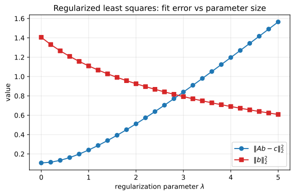
The regularization trade-off for Problem 4.3. As \(\lambda\) sweeps from 0 to 5, the squared fit error \(\|Ab-c\|_2^2\) rises monotonically from 3/28 to 1.56 while the squared parameter size \(\|b\|_2^2\) falls monotonically from 1.41 to 0.61. The two curves cross near \(\lambda \approx 2.9\).
The two curves move monotonically in opposite directions: \(\mathbf{b}(\lambda)\) traces the Pareto frontier of the two objectives, with \(\lambda\) the exchange rate between them. The rate is what matters. Going from \(\lambda=0\) to \(\lambda=1\) buys a \(21\%\) cut in \(\|\mathbf{b}\|_2^2\) for \(0.13\) of fit error, while \(\lambda=4\) to \(\lambda=5\) buys only \(12\%\) for \(0.37\) — which is why the test-error curve of Figure 4.9 is U-shaped, early shrinkage removing variance almost free while past the optimum the induced bias dominates. Without held-out data the plot shows the trade-off but not where to sit on it; that needs the cross-validation of Section 4.4.1.
Problem 4.4 — Convex functions
Convex functions. Determine whether the following functions are convex, concave, both, or neither:
- (a) \(f(x)=3x+4\), for all real \(x\);
- (b) \(f(x)=4\ln(x/3)\), for all \(x>0\);
- (c) \(f(x)=e^{2x}\), for all real \(x\);
- (d) \(f(x,y)=-3x^2-4y^2\), for all real \(x\) and \(y\);
- (e) \(f(x,y)=xy\), for all real \(x\) and \(y\).
(difficulty: \(\star\))
(a) both; (b) concave; (c) convex; (d) concave; (e) neither. By the Section 4.2.2 test, a twice-differentiable \(f\) on a convex domain is convex iff its Hessian is positive semidefinite everywhere and concave iff it is negative semidefinite; every domain here (\(\mathbb{R}\), \(\mathbb{R}_{>0}\), \(\mathbb{R}^2\)) is convex, so only the Hessian matters.
(a) \(f^{\prime\prime}(x)=0\) is simultaneously \(\ge 0\) and \(\le 0\), so \(f\) is both — and being both forces \(f^{\prime\prime}\equiv 0\), hence \(f\) affine.
(b) Writing \(f(x)=4\ln x-4\ln 3\) gives \(f^{\prime\prime}(x)=-4/x^2<0\) on \(x>0\): strictly concave.
(c) \(f^{\prime\prime}(x)=4e^{2x}>0\) for all real \(x\): strictly convex.
(d) Strictly concave, the Hessian being the constant matrix
\begin{equation*} \nabla^2 f=\begin{bmatrix}-6&0\\0&-8\end{bmatrix}, \end{equation*}
with eigenvalues \(-6\) and \(-8\), hence negative definite.
(e) Neither: the Hessian is
\begin{equation*} \nabla^2 f=\begin{bmatrix}0&1\\1&0\end{bmatrix}, \end{equation*}
with eigenvalues \(+1\) and \(-1\), indefinite. Witness: \((1,1)\) and \((-1,-1)\) both give \(f=1\) with midpoint value \(0<1\), ruling out concavity, while \((1,-1)\) and \((-1,1)\) both give \(f=-1\) with midpoint value \(0>-1\), ruling out convexity.
import numpy as np
import sympy as sp

x, y = sp.symbols('x y', real=True)
cases = {
    '(a) 3x+4':        (3*x + 4, [x]),
    '(b) 4 ln(x/3)':   (4*sp.log(x/3), [x]),
    '(c) exp(2x)':     (sp.exp(2*x), [x]),
    '(d) -3x^2-4y^2':  (-3*x**2 - 4*y**2, [x, y]),
    '(e) xy':          (x*y, [x, y]),
}
for name, (f, vs) in cases.items():
    H = sp.hessian(f, vs)
    ev = sorted(sp.Matrix(H).eigenvals().keys(), key=str)
    print(f"{name:16s} Hessian = {sp.simplify(H).tolist()}   eigenvalues = {ev}")
(a) 3x+4         Hessian = [[0]]   eigenvalues = [0]
(b) 4 ln(x/3)    Hessian = [[-4/x**2]]   eigenvalues = [-4/x**2]
(c) exp(2x)      Hessian = [[4*exp(2*x)]]   eigenvalues = [4*exp(2*x)]
(d) -3x^2-4y^2   Hessian = [[-6, 0], [0, -8]]   eigenvalues = [-6, -8]
(e) xy           Hessian = [[0, 1], [1, 0]]   eigenvalues = [-1, 1]
Case (e) is why the latent-factor objective (4.8), bilinear in \(\mathbf{p}_u^T\mathbf{q}_i\) across both sets of variables, is not convex and needs the alternating projections of Section 4.4.2.
Problem 4.5 — Log-Sum-Exp and geometric programming
Log-Sum-Exp and geometric programming.
- (a) Is \(\exp(x+y)\) convex or concave in \((x,y)\)?
- (b) Is \(\exp(x+y)+\exp(2x+5y)\) convex or concave in \((x,y)\)?
- (c) Is \(\log(\exp(x+y)+\exp(2x+5y))\) convex or concave in \((x,y)\)? This log-sum-exp function is heavily used in a class of convex optimization called geometric programming in fields like statistical physics, chemical engineering, communication systems, and circuit design.
- (d) Can you turn the following problem in variables \(x,y,z>0\) into convex optimization?
\begin{equation*} \begin{aligned} \text{minimize}\quad & xy+xz\\ \text{subject to}\quad & x^2yz+xz^{-1}\le 10\\ & 0.5\,x^{-0.5}y^{-1}=1 . \end{aligned} \end{equation*}
(Hint: try a log change of variables.)
(difficulty: \(\star\star\))
(a) Convex, not concave: \(e^{s}\) is convex in the scalar \(s\) (Problem 4.4(c)) and \(s=x+y\) is affine in \((x,y)\), and convexity survives precomposition with an affine map. Directly,
\begin{equation*} \nabla^2 f=e^{x+y}\begin{bmatrix}1&1\\1&1\end{bmatrix}, \end{equation*}
whose eigenvalues \(2e^{x+y}>0\) and \(0\) make it positive semidefinite but not negative semidefinite. It is singular because \(f\) depends on \((x,y)\) only through \(x+y\), leaving it flat along \((1,-1)\).
(b) Convex, not concave, as a non-negative sum of the convex functions \(e^{x+y}\) and \(e^{2x+5y}\). Convexity is in fact strict: the two Hessians are rank-one with independent null directions \((1,-1)\) and \((5,-2)\), so their sum is positive definite — confirmed below by \(\operatorname{tr}=2e^{x+y}+29e^{2x+5y}>0\) and \(\det=9e^{3x+6y}>0\).
(c) Convex, not concave. Generally \(g(\mathbf{z})=\log\sum_{k=1}^{n}e^{z_k}\) is convex on \(\mathbb{R}^n\): with \(p_k=e^{z_k}/\sum_j e^{z_j}\), so \(p_k>0\) and \(\sum_k p_k=1\), we get \(\partial g/\partial z_k=p_k\) and
\begin{equation*} \nabla^2 g=\operatorname{diag}(\mathbf{p})-\mathbf{p}\mathbf{p}^T . \end{equation*}
For any \(\mathbf{v}\),
\begin{equation*} \mathbf{v}^T\nabla^2 g\,\mathbf{v}=\sum_k p_k v_k^2-\Big(\sum_k p_k v_k\Big)^2\;\ge\;0, \end{equation*}
this being the non-negativity of the variance of the variable taking \(v_k\) with probability \(p_k\). So \(\nabla^2 g\succeq 0\), and composing with the affine \((x,y)\mapsto(x+y,\,2x+5y)\) preserves convexity. It is not concave: the trace \(17e^{x+4y}/(1+e^{x+4y})^2>0\) forces a strictly positive eigenvalue. Note (c) does not follow from (b), since \(\log\) is concave and \(\log(\text{convex})\) need not be convex; the variance argument is what supplies it.
import sympy as sp

x, y = sp.symbols('x y', real=True)
g1 = sp.exp(x + y)
g2 = sp.exp(x + y) + sp.exp(2*x + 5*y)
g3 = sp.log(g2)
for name, f in [('(a) e^(x+y)', g1), ('(b) e^(x+y)+e^(2x+5y)', g2),
                ('(c) log-sum-exp', g3)]:
    H = sp.simplify(sp.hessian(f, [x, y]))
    print(name)
    print("   trace =", sp.simplify(H.trace()))
    print("   det   =", sp.simplify(H.det()))
(a) e^(x+y)
   trace = 2*exp(x + y)
   det   = 0
(b) e^(x+y)+e^(2x+5y)
   trace = 2*exp(x + y) + 29*exp(2*x + 5*y)
   det   = 9*exp(3*x + 6*y)
(c) log-sum-exp
   trace = 17*exp(x + 4*y)/(2*exp(x + 4*y) + exp(2*x + 8*y) + 1)
   det   = 0
For a symmetric \(2\times 2\) matrix, non-negative trace with non-negative determinant is positive semidefiniteness, so all three are convex, and all three traces are strictly positive, so none is concave.
(d) Yes — the problem is a geometric program, its objective and inequality left side being posynomials and its equality constraint a monomial. Substitute
\begin{equation*} x=e^{u},\qquad y=e^{v},\qquad z=e^{w},\qquad (u,v,w)\in\mathbb{R}^3 , \end{equation*}
a bijection onto the open orthant \(x,y,z>0\), under which every monomial becomes an exponential of an affine function:
\begin{equation*} xy=e^{u+v},\quad xz=e^{u+w},\quad x^2yz=e^{2u+v+w},\quad xz^{-1}=e^{u-w},\quad 0.5x^{-0.5}y^{-1}=e^{\ln 0.5-0.5u-v}. \end{equation*}
Since \(\log\) is strictly increasing, taking logarithms leaves both the minimizer and the feasible set unchanged:
\begin{equation*} \begin{aligned} \text{minimize}_{u,v,w}\quad & \log\!\left(e^{u+v}+e^{u+w}\right)\\ \text{subject to}\quad & \log\!\left(e^{2u+v+w}+e^{u-w}\right)\le \log 10\\ & 0.5u+v=\ln 0.5 = -\ln 2 . \end{aligned} \end{equation*}
Objective and inequality left side are log-sum-exp of affine maps, hence convex by (c); a sublevel set of a convex function is convex (Figure 4.5); and the affine equality defines a hyperplane. Minimizing a convex function over an intersection of convex sets is convex optimization, so every local optimum is global.
The infimum is nevertheless not attained. Eliminating \(y=\tfrac12 x^{-1/2}\) by the equality turns the objective into \(\tfrac12 x^{1/2}+xz\) and the inequality into \(\tfrac12 x^{3/2}z+x/z\le 10\); along the feasible family \(z=x/9\) the inequality reads \(\tfrac{1}{18}x^{5/2}+9\le 10\), true for all small \(x\), while the objective \(\tfrac12 x^{1/2}+\tfrac19 x^2\to 0\). So the infimum is \(0\), approached as \(u\to-\infty\) along a feasible ray.
for xv in [1e-1, 1e-2, 1e-3, 1e-4]:
    yv = 0.5 * xv**-0.5
    zv = xv / 9.0
    lhs = xv**2 * yv * zv + xv / zv
    print(f"x={xv:g}  y={yv:g}  z={zv:g}  |  0.5 x^-0.5 y^-1 = {0.5*xv**-0.5/yv:.1f}"
          f"  |  constraint LHS = {lhs:.4f} <= 10"
          f"  |  objective xy+xz = {xv*yv+xv*zv:.6f}")
x=0.1  y=1.58114  z=0.0111111  |  0.5 x^-0.5 y^-1 = 1.0  |  constraint LHS = 9.0002 <= 10  |  objective xy+xz = 0.159225
x=0.01  y=5  z=0.00111111  |  0.5 x^-0.5 y^-1 = 1.0  |  constraint LHS = 9.0000 <= 10  |  objective xy+xz = 0.050011
x=0.001  y=15.8114  z=0.000111111  |  0.5 x^-0.5 y^-1 = 1.0  |  constraint LHS = 9.0000 <= 10  |  objective xy+xz = 0.015811
x=0.0001  y=50  z=1.11111e-05  |  0.5 x^-0.5 y^-1 = 1.0  |  constraint LHS = 9.0000 <= 10  |  objective xy+xz = 0.005000
The original problem is not convex in \((x,y,z)\) — its objective carries the indefinite bilinear term of Problem 4.4(e) — yet the change of variables shows it was convex all along, merely written in the wrong coordinates.
When can I trust an average rating on Amazon?
Problem 5.1 — Bayesian ranking
Bayesian ranking. Suppose there are 50 ratings for all printers, with an average rating of 4. Given ratings 5, 5, and 5 for a printer by Canon, and ratings 4.5, 5, 4, 5, 4, 5, 3, 5, 4.5, and 3.5 for another by HP, calculate the ranking by average rating and the Bayesian ranking, respectively. (difficulty: \(\star\))
By raw average Canon (5.00) leads HP (4.35); the Bayesian ranking flips the order, HP (4.0583) over Canon (4.0566). The rule is equation (5.5),
\begin{equation*} \tilde r_i \;=\; \frac{N R + n_i r_i}{N + n_i}, \end{equation*}
with \(R\) the average across comparable products, \(N\) the review population attached to that prior, and \(n_i, r_i\) the product’s review count and raw average. The problem hands over the prior: \(N = 50\), \(R = 4\), so \(NR = 200\). Canon’s \(n_C = 3\) ratings are all 5, so \(r_C = 5\); HP’s \(n_H = 10\) sum to \(43.5\), so \(r_H = 4.35\). Hence
\begin{equation*} \tilde r_C = \frac{200 + 3\times 5}{50+3} = \frac{215}{53} = 4.0566, \qquad \tilde r_H = \frac{200 + 43.5}{50+10} = \frac{243.5}{60} = 4.0583. \end{equation*}
Canon’s perfect score rests on three reviews, so the adjustment drags it almost all the way back to the prior \(R=4\), while HP’s ten reviews keep more of its \(0.35\)-point surplus.
import numpy as np

N, R = 50, 4.0                     # prior population, prior mean rating
canon = np.array([5, 5, 5], dtype=float)
hp    = np.array([4.5, 5, 4, 5, 4, 5, 3, 5, 4.5, 3.5])

def bayes(r, n, N=N, R=R):
    return (N*R + n*r) / (N + n)

for name, v in [('Canon', canon), ('HP', hp)]:
    n, r = len(v), v.mean()
    print(f"{name}: n={n}  raw mean r={r:.4f}  n*r={n*r:.2f}  Bayesian={bayes(r,n):.6f}")
print("gap (HP - Canon) =", bayes(hp.mean(), len(hp)) - bayes(canon.mean(), len(canon)))
Canon: n=3  raw mean r=5.0000  n*r=15.00  Bayesian=4.056604
HP: n=10  raw mean r=4.3500  n*r=43.50  Bayesian=4.058333
gap (HP - Canon) = 0.0017295597484281444
The margin is 0.0017 stars, so the verdict turns on the choice of \(N\) — Section 5.3.3 shows \(N_{\min}\), \(N_{\max}\), \(N_{\text{ave}}\), \(N_{\text{sum}}\) giving four different rankings of the same twenty HDTVs. Sweeping \(N\) with \(R = 4\):
R = 4.0
def bayes_N(r, n, N):
    return (N*R + n*r) / (N + n)

print(" N    Canon(3,5.00)  HP(10,4.35)   winner")
for N in [5, 10, 20, 30, 38, 39, 40, 50, 100, 200]:
    c, h = bayes_N(5.0, 3, N), bayes_N(4.35, 10, N)
    print(f"{N:4d}   {c:.5f}        {h:.5f}       {'Canon' if c > h else 'HP'}")
N    Canon(3,5.00)  HP(10,4.35)   winner
  5   4.37500        4.23333       Canon
 10   4.23077        4.17500       Canon
 20   4.13043        4.11667       Canon
 30   4.09091        4.08750       Canon
 38   4.07317        4.07292       Canon
 39   4.07143        4.07143       HP
 40   4.06977        4.07000       HP
 50   4.05660        4.05833       HP
100   4.02913        4.03182       HP
200   4.01478        4.01667       HP
Solving \((4N+15)/(N+3) = (4N+43.5)/(N+10)\) puts the crossover at \(N = 39\), the two tied at \(4.0714\) (the table’s strict-inequality tie-break prints HP there). Below 39 Canon keeps the top spot, above it HP takes over, and the stated \(N = 50\) sits just past that boundary — a prior population of 38 would have reversed the reversal.
Problem 5.2 — Analyzing Amazon data
Analyzing Amazon data. Take a look at the rating data in worksheet “raw” of the following file: http://www.network20q.com/hw/amazon_data.xls for the iPod touch, address the following.
- (a)
- Compute the mean and the adjusted mean. Here, we define the adjusted mean as \(\sum(\text{rating}\times\text{number of helpful reviews})/\text{total number of helpful reviews}\).
- (b)
- Plot the monthly mean.
- (c)
- How does the temporal pattern of the monthly mean influence your perception of the product quality?
- (d)
- Which metric (raw mean, adjusted mean, or monthly mean) is the most accurate in your opinion? Would a certain combination of the metrics be more useful?
(difficulty: \(\star\star\star\))
Data availability. The file is unrecoverable: amazon_data.xls returns 404, network20q.com was already a parked redirect at its first Wayback capture, and no mirror survives. Every number below comes from a surrogate I generated, calibrated to the one quantitative fact the chapter states about this dataset (Example 3, Figure 5.2: the 60 most recent ratings average about 1.5 times the 60 most helpful) and shaped like curve (c) of Figure 5.3 — the unconverged case, the only one for which parts (c) and (d) have content. The digits are illustrative; the shape is the answer.
Three ingredients drive the generator: the per-month rating distribution drifts upward over the two-year window; helpful votes accumulate with exposure time, so a month-1 review has had 24 months to collect them and last week’s has had days; and critical reviews are more salient, given a \(1.7\) multiplier for 1–2 star reviews plus a lognormal review-quality factor so the most-helpful set is a genuine mixture.
import numpy as np, pandas as pd

rng = np.random.default_rng(52)
months = pd.period_range('2010-01', '2011-12', freq='M')
n_m = len(months)
rows = []
for k, m in enumerate(months):
    t = k / (n_m - 1)
    n_rev = int(rng.integers(18, 34))
    p_bad = 0.45 * (1 - t) ** 1.5 + 0.04           # teething phase early, fades
    for _ in range(n_rev):
        if rng.random() < p_bad:
            r = int(rng.choice([1, 2, 3], p=[0.55, 0.30, 0.15]))
        else:
            r = int(rng.choice([4, 5], p=[0.30, 0.70]))
        age = n_m - k                               # months of exposure to voters
        salience = 1.7 if r <= 2 else (1.2 if r == 3 else 1.0)
        quality  = rng.lognormal(0.0, 0.95)         # idiosyncratic review quality
        h = int(rng.poisson(0.9 * age * salience * quality))
        rows.append((m.to_timestamp(), r, h))

df = pd.DataFrame(rows, columns=['date', 'rating', 'helpful'])

raw = df.rating.mean()
adj = (df.rating * df.helpful).sum() / df.helpful.sum()
print("reviews: %d   helpful votes: %d" % (len(df), df.helpful.sum()))
print("raw mean       = %.4f" % raw)
print("adjusted mean  = %.4f" % adj)
print("adjusted - raw = %+.4f" % (adj - raw))
h60 = df.nlargest(60, 'helpful'); r60 = df.sort_values('date').tail(60)
print("mean of 60 most-helpful = %.4f" % h60.rating.mean())
print("mean of 60 most-recent  = %.4f" % r60.rating.mean())
print("ratio recent/helpful    = %.3f" % (r60.rating.mean() / h60.rating.mean()))
c = np.corrcoef(df.helpful, (df.date - df.date.min()).dt.days)[0, 1]
print("corr(helpful votes, review recency) = %+.3f" % c)
reviews: 596   helpful votes: 12622
raw mean       = 3.9765
adjusted mean  = 3.3257
adjusted - raw = -0.6508
mean of 60 most-helpful = 2.8500
mean of 60 most-recent  = 4.6167
ratio recent/helpful    = 1.620
corr(helpful votes, review recency) = -0.400
(a) Raw mean 3.98, adjusted mean 3.33, with the recent-to-helpful ratio at 1.62 against the chapter’s 1.5. The 0.65-star gap is the point: helpful-vote count correlates \(-0.40\) with recency here, so helpfulness is substantially a proxy for age, and the adjusted mean overweights the oldest cohort, which is also the angriest. Add salience and both biases pull the same way. Despite its name it is a re-weighting, not a correction: \(\sum h_i r_i/\sum h_i\) answers “what did the reviews people found useful say?”, not “how good is this product?”
(b) Monthly mean.
import matplotlib.pyplot as plt

g       = df.groupby('date')
monthly = g['rating'].mean()
cnt     = g['rating'].count()
srt     = df.sort_values('date')
cum     = srt['rating'].expanding().mean().groupby(srt['date']).last()
roll3   = monthly.rolling(3).mean()

fig, ax = plt.subplots(2, 1, figsize=(9, 6.6), sharex=True,
                       gridspec_kw={'height_ratios': [3, 1]})
ax[0].plot(monthly.index, monthly.values, 'o-', lw=1.2, ms=4, color='#3b6ea5', label='monthly mean')
ax[0].plot(roll3.index, roll3.values, lw=2.2, color='#c1440e', label='3-month moving average')
ax[0].plot(cum.index, cum.values, lw=1.6, ls='--', color='#2f7d32', label='cumulative mean')
ax[0].axhline(raw, color='k', lw=1.0, ls=':', label='raw mean = %.2f' % raw)
ax[0].axhline(adj, color='#8e44ad', lw=1.0, ls='-.', label='adjusted mean = %.2f' % adj)
ax[0].set_ylabel('rating'); ax[0].set_ylim(1, 5.2)
ax[0].legend(fontsize=8, ncol=2, loc='lower right')
ax[0].set_title('iPod touch surrogate: monthly vs aggregate rating metrics')
ax[1].bar(cnt.index, cnt.values, width=20, color='#9aa5b1')
ax[1].set_ylabel('reviews'); ax[1].set_xlabel('month')
plt.tight_layout()
plt.savefig('nl-ch05-monthly-mean.svg', dpi=150, bbox_inches='tight')

print("year 1 mean = %.4f    year 2 mean = %.4f"
      % (df[df.date < '2011-01-01'].rating.mean(), df[df.date >= '2011-01-01'].rating.mean()))
print("last 3 months mean = %.4f" % df[df.date >= '2011-10-01'].rating.mean())
print("monthly mean: min %.3f  max %.3f  sd %.3f" % (monthly.min(), monthly.max(), monthly.std()))
year 1 mean = 3.5724    year 2 mean = 4.3779
last 3 months mean = 4.5946
monthly mean: min 3.107  max 4.842  sd 0.517
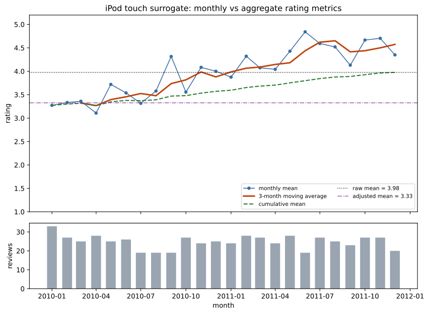
Monthly mean rating for the surrogate iPod touch data, with a 3-month moving average, the running cumulative mean, and the two scalar summaries (raw mean 3.98, helpfulness-adjusted mean 3.33) drawn as horizontal reference lines. The lower panel shows the monthly review count, so the reader can see which points are thin.
(c) It reverses the reading. As a scalar this is a 3.98, or 3.33 under helpfulness weighting: mediocre-to-decent. As a series it started at 3.1–3.4 and now runs at 4.6, year 2 (4.38) beating year 1 (3.57) by 0.8 stars. (i) The trend dominates the level: a buyer today cares about the distribution generating today’s reviews, best estimated by the recent window at 4.59, not a pooled mean over a distribution that no longer exists. (ii) The cumulative mean is still climbing at the right edge of the plot — a lagging indicator whose memory horizon is the entire product lifetime. (iii) The diagnosis changes, not just the number: a flat 3.98 with high variance means a polarising product (Example 2, the Pyle Home speaker), while a rise from 3.1 to 4.6 means an early defect since fixed. The caution is that this reading assumes a stable reviewer population; early adopters and late mainstream buyers have different baselines, so a rising curve may be composition change, or the manipulation signature of Section 5.3.3 item 3(d).
(d) None of the three; use a Bayesian-shrunk recent window. Ranked worst to best: the adjusted mean fails by bias, not variance, scoring 3.33 against a current level near 4.6 because its weights load on the oldest and most negative reviews — defensible only if votes were normalised by exposure time. The raw mean is the honest baseline, unbiased for the pooled history, which is the wrong target under non-stationarity but the right one for a flat series (Figure 5.3(b)). The monthly mean asks the right question with the worst variance: sd \(0.517\) across months of only 18–34 reviews, so the latest month is a 20-sample estimate. Combining the two halves the chapter already supplies — a recent window for the non-stationarity, equation (5.5)’s shrinkage for the resulting variance:
\begin{equation*} \hat r_{\text{best}} \;=\; \frac{N R + n_W \, r_W}{N + n_W}, \end{equation*}
with \(r_W\) the mean over a trailing window \(W\), \(n_W\) its review count, \(R\) the category average and \(N\) its population. The window length sets how much stale data is admitted (bias) and the shrinkage absorbs the small \(n_W\) a short window leaves (variance), so Section 5.1.2’s open question of window size is exactly the bias-variance knob; the two compose because (5.5) does not care where \(r_i\) came from. Publish it with \(n_W\) and the trend slope rather than as a bare scalar, and apply helpfulness only within the window, where the exposure-time confound is nearly constant.
The chapter’s single real-data anchor — the 1.5 ratio of recent to helpful means — is matched by the surrogate at 1.62, and that fact alone forces the structure of (c) and (d): the real series is non-stationary with recent ratings well above helpful-weighted ones, so there too the adjusted mean lags the raw mean and both lag the recent level. Only the specific digits in (a) and (b) are uncertifiable against the vanished file.
Problem 5.3 — Averaging a crowd
Averaging a crowd. Suppose the estimation errors \(\{\epsilon_i\}\) are independent and identically distributed random variables that takes values 1 and \(-1\) with an equal probability. \(X\) is a uniform random variable that takes on 100 possible values (\(P(X=x) = 1/100\), \(x = 1, 2, \ldots, 100\)). Calculate \(E_{AE}\) and \(E_{EA}\) for \(N = 100\). Does the relationship between \(E_{AE}\) and \(E_{EA}\) hold?
Now let \(N = 1000\) and let \(X\) take on 1000 possible values uniformly. Plot the histogram of \(\frac{1}{N}\sum_{i=1}^{N}\epsilon_i(x)\) over all trials of \(X\). What kind of distribution is the histogram? What is the variance? How does this relate to \(E_{EA}\)? (difficulty: \(\star\))
\(E_{AE} = 1\) and \(E_{EA} = 1/N = 0.01\), so equation (5.3) holds with equality. The errors are Rademacher, \(P(\epsilon_i = \pm 1) = 1/2\), independent across \(i\) and across \(x\); their law does not depend on \(x\), so the uniform \(X\) is scaffolding for the simulation and plays no part in the algebra. Since \(\epsilon_i \in \{-1,+1\}\) makes \(\epsilon_i^2 \equiv 1\) deterministically, equation (5.1) gives
\begin{equation*} E_{AE} \;=\; \frac{1}{N}\sum_{i=1}^{N}\mathbf{E}_x\!\left[\epsilon_i^2(x)\right] \;=\; \frac{1}{N}\cdot N \cdot 1 \;=\; 1 . \end{equation*}
— an individual guess is wrong by exactly 1 every time, independent of \(N\). Equation (5.2) then gives
\begin{equation*} E_{EA} \;=\; \frac{1}{N^2}\,\mathbf{E}_x\!\left[\Big(\sum_{i=1}^{N}\epsilon_i(x)\Big)^{2}\right] \;=\; \frac{1}{N^2}\left(\sum_{i}\mathbf{E}[\epsilon_i^2] + \sum_{i \neq j}\mathbf{E}[\epsilon_i \epsilon_j]\right). \end{equation*}
Independence and zero mean kill every cross-term, \(\mathbf{E}[\epsilon_i \epsilon_j] = 0\) for \(i \neq j\), leaving the \(N\) diagonal terms:
\begin{equation*} E_{EA} \;=\; \frac{1}{N^2}\cdot N \;=\; \frac{1}{N} \;=\; \frac{1}{100} \;=\; 0.01 . \end{equation*}
Equation (5.3)’s \(E_{EA} = E_{AE}/N\) therefore holds with equality, its hypotheses — independent, unbiased errors — being met exactly: the crowd of 100 cuts MSE by a factor of 100 and RMSE by 10. Confirming by simulation:
import numpy as np
rng = np.random.default_rng(53)

N, M = 100, 100                                 # crowd size, number of x-values
eps = rng.choice([-1.0, 1.0], size=(M, N))      # eps[x, i]
E_AE = np.mean([np.mean(eps[:, i] ** 2) for i in range(N)])
E_EA = np.mean(eps.mean(axis=1) ** 2)
print("N = 100")
print("  E_AE (empirical) = %.6f      theory = 1" % E_AE)
print("  E_EA (empirical) = %.6f      theory = 1/N = %.6f" % (E_EA, 1/N))
print("  E_EA / E_AE      = %.6f" % (E_EA / E_AE))
N = 100
  E_AE (empirical) = 1.000000      theory = 1
  E_EA (empirical) = 0.010084      theory = 1/N = 0.010000
  E_EA / E_AE      = 0.010084
\(E_{AE}\) is exactly \(1.000000\) with no sampling error, since \(\epsilon_i^2 \equiv 1\) is an identity rather than an expectation; the residual in \(E_{EA} = 0.010084\) is Monte Carlo error from only 100 trials of \(X\), of the expected relative order \(1/\sqrt{100}\).
The histogram for a crowd of 1000.
import numpy as np
import matplotlib.pyplot as plt
from scipy import stats

rng = np.random.default_rng(531)
N, M = 1000, 1000                          # crowd size, number of x values
eps  = rng.choice([-1.0, 1.0], size=(M, N))
abar = eps.mean(axis=1)                    # (1/N) sum_i eps_i(x), one per trial x

print("mean of abar     = %+.6f   (theory 0)" % abar.mean())
print("variance of abar = %.6f    (theory 1/N = %.6f)" % (abar.var(), 1/N))
print("std of abar      = %.6f    (theory 1/sqrt(N) = %.6f)" % (abar.std(), 1/np.sqrt(N)))
print("E_EA empirical   = %.6f    (= mean of abar^2)" % (abar**2).mean())
print("E_AE empirical   = %.6f" % (eps**2).mean())
print("Shapiro-Wilk p   = %.4f" % stats.shapiro(abar).pvalue)

fig, ax = plt.subplots(figsize=(7.5, 4.4))
ax.hist(abar, bins=41, density=True, color='#9ec3e6', edgecolor='#3b6ea5', label='empirical')
xs = np.linspace(abar.min(), abar.max(), 400)
ax.plot(xs, stats.norm.pdf(xs, 0, 1/np.sqrt(N)), color='#c1440e', lw=2.2,
        label=r'$\mathcal{N}(0, 1/N)$')
ax.set_xlabel(r'$\frac{1}{N}\sum_{i=1}^{N}\epsilon_i(x)$')
ax.set_ylabel('density')
ax.set_title('Averaged error over 1000 trials of X, crowd size N = 1000')
ax.legend()
plt.savefig('nl-ch05-crowd-histogram.svg', dpi=150, bbox_inches='tight')
mean of abar     = +0.001726   (theory 0)
variance of abar = 0.001056    (theory 1/N = 0.001000)
std of abar      = 0.032492    (theory 1/sqrt(N) = 0.031623)
E_EA empirical   = 0.001059    (= mean of abar^2)
E_AE empirical   = 1.000000
Shapiro-Wilk p   = 0.0190
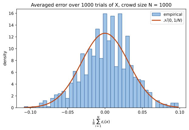
Histogram of the averaged error over 1000 trials of X with crowd size N = 1000, against the normal density with mean 0 and variance 1/N. The Gaussian envelope is the central limit theorem acting on 1000 Rademacher errors; the alternating bar heights are a lattice artifact, since the sample mean lives on a grid of spacing 2/N = 0.002 that the 0.005-wide bins do not divide evenly.
The histogram is Gaussian. Exactly, \(\frac{1}{N}\sum_i \epsilon_i = (2S-N)/N\) with \(S \sim \mathrm{Bin}(N,1/2)\) the number of \(+1\)s, supported on the lattice of spacing \(2/N\); the central limit theorem sends it to \(\mathcal{N}(0, 1/N)\), already excellent at \(N = 1000\). The sawtooth in the bar heights is that lattice beating against the binning, and the Shapiro-Wilk \(p = 0.019\) is detecting the same discreteness, not skew or heavy tails.
The measured variance is \(0.001056\) against the theoretical \(1/N = 0.001\), and since the crowd is unbiased,
\begin{equation*} E_{EA} \;=\; \mathbf{E}\!\left[\Big(\tfrac{1}{N}\sum_i \epsilon_i\Big)^{2}\right] \;=\; \mathrm{Var}\!\left(\tfrac{1}{N}\sum_i \epsilon_i\right) + \Big(\mathbf{E}\big[\tfrac{1}{N}\sum_i \epsilon_i\big]\Big)^{2} \;=\; \mathrm{Var}\!\left(\tfrac{1}{N}\sum_i \epsilon_i\right) + 0 . \end{equation*}
so \(E_{EA}\) is the variance of the histogram: \(0.001059\) empirical against \(0.001056\), agreeing to four decimals. Averaging shrinks only that variance term: give the crowd any common bias \(b\) and the same algebra gives \(E_{EA} = b^2 + 1/N\), which floors at \(b^2\) however many reviewers are gathered — the caution on page 95 that averaging cannot reduce a bias everyone shares.
Problem 5.4 — Averaging a dependent crowd
Averaging a dependent crowd. Consider three people making dependent estimates of a number, with the following expectations of errors and correlations of errors:
\begin{equation*} \mathbf{E}[\epsilon_1^2] = 1773, \quad \mathbf{E}[\epsilon_2^2] = 645, \quad \mathbf{E}[\epsilon_3^2] = 1796, \end{equation*}
\begin{equation*} \mathbf{E}[\epsilon_1 \epsilon_2] = 1057, \quad \mathbf{E}[\epsilon_1 \epsilon_3] = 970, \quad \mathbf{E}[\epsilon_2 \epsilon_3] = 708. \end{equation*}
Compute the average of errors and the error of the average in this case. (difficulty: \(\star\star\))
\(E_{AE} = 4214/3 \approx 1404.67\) and \(E_{EA} = 1076\) exactly. Equation (5.1) uses only the diagonal second moments,
\begin{equation*} E_{AE} \;=\; \frac{1}{N}\sum_{i=1}^{3}\mathbf{E}[\epsilon_i^2] \;=\; \frac{1773 + 645 + 1796}{3} \;=\; \frac{4214}{3} \;=\; 1404.67 . \end{equation*}
while in equation (5.2) the cross-terms survive, the estimates being dependent:
\begin{equation*} \Big(\sum_{i=1}^{3}\epsilon_i\Big)^{2} = \epsilon_1^2 + \epsilon_2^2 + \epsilon_3^2
- 2\epsilon_1\epsilon_2 + 2\epsilon_1\epsilon_3 + 2\epsilon_2\epsilon_3 , \end{equation*}
so
\begin{equation*} \begin{aligned} E_{EA} &\;=\; \frac{1}{N^2}\,\mathbf{E}\!\left[\Big(\sum_{i}\epsilon_i\Big)^{2}\right] \;=\; \frac{1}{9}\Big[(1773+645+1796) + 2(1057+970+708)\Big] \\ &\;=\; \frac{4214 + 5470}{9} \;=\; \frac{9684}{9} \;=\; 1076 . \end{aligned} \end{equation*}
Compactly, with the second-moment matrix \(C_{ij} = \mathbf{E}[\epsilon_i \epsilon_j]\), we have \(E_{AE} = \operatorname{tr}( C)/N\) and \(E_{EA} = \mathbf{1}^{\!\top} C \,\mathbf{1}/N^2\), the two differing by exactly the off-diagonal mass.
import numpy as np
from fractions import Fraction as F

C = np.array([[1773, 1057,  970],
              [1057,  645,  708],
              [ 970,  708, 1796]], float)      # C[i,j] = E[eps_i eps_j]
N = 3
E_AE = np.trace(C) / N
E_EA = C.sum() / N**2
print("E_AE = (1/3) * %d = %.4f   exact %s" % (int(np.trace(C)), E_AE, F(int(np.trace(C)), 3)))
print("E_EA = (1/9) * %d = %.4f   exact %s" % (int(C.sum()), E_EA, F(int(C.sum()), 9)))
print("E_EA / E_AE            = %.4f" % (E_EA / E_AE))
print("independent case (1/N) = %.4f" % (1/N))
print("fully dependent case   = 1.0000")
print("effective crowd size N_eff = E_AE/E_EA = %.4f" % (E_AE / E_EA))
print("RMSE: individual %.3f -> average %.3f" % (np.sqrt(E_AE), np.sqrt(E_EA)))
sd = np.sqrt(np.diag(C))
print("std devs:", np.round(sd, 3))
print("correlation matrix:\n", np.round(C / np.outer(sd, sd), 4))
print("eigenvalues of C:", np.round(np.linalg.eigvalsh(C), 3))
E_AE = (1/3) * 4214 = 1404.6667   exact 4214/3
E_EA = (1/9) * 9684 = 1076.0000   exact 1076
E_EA / E_AE            = 0.7660
independent case (1/N) = 0.3333
fully dependent case   = 1.0000
effective crowd size N_eff = E_AE/E_EA = 1.3055
RMSE: individual 37.479 -> average 32.802
std devs: [42.107 25.397 42.379]
correlation matrix:
 [[1.     0.9884 0.5436]
 [0.9884 1.     0.6578]
 [0.5436 0.6578 1.    ]]
eigenvalues of C: [1.194000e+00 8.755240e+02 3.337282e+03]
Page 95’s extremes are \(E_{EA} = E_{AE}/N\) under full independence and \(E_{EA} = E_{AE}\) under full dependence; this crowd sits at \(E_{EA}/E_{AE} = 0.766\) against the \(0.333\) independence would have bought, so the effective crowd size is \(N_{\text{eff}} = E_{AE}/E_{EA} = 1.31\) and the individual RMSE of 37.5 falls only to 32.8. The correlation matrix says why: \(\epsilon_1\) and \(\epsilon_2\) correlate \(0.988\), so persons 1 and 2 are statistically one person and only person 3 contributes fresh information. Worse, person 2 is the best individual estimator (\(645\) against 1773 and 1796), so uniform averaging drags the good estimate toward two bad and redundant ones: its MSE of 1076 is worse than listening to person 2 alone.
The best linear unbiased combination, \(w \propto C^{-1}\mathbf{1}\) normalised, reports weights \((-1.49, 2.77, -0.28)\) and an MSE of \(12.07\) — which I do not trust. The eigenvalues of \(C\) run from \(1.194\) to \(3337\), a condition number near 2800, so \(C\) sits almost exactly on the boundary of the positive-semidefinite cone; perturbing one printed moment by under 1% either raises the minimum MSE sevenfold or pushes \(C\) out of the cone, giving an impossible negative MSE:
import numpy as np
C = np.array([[1773, 1057, 970], [1057, 645, 708], [970, 708, 1796]], float)
o = np.ones(3)

def opt(M):
    ci = np.linalg.inv(M)
    return ci @ o / (o @ ci @ o), 1 / (o @ ci @ o)

w0, m0 = opt(C)
print("as printed:            weights %s   MSE %8.3f   min eig %8.3f"
      % (np.round(w0, 3), m0, np.linalg.eigvalsh(C).min()))
for lbl, (i, j, d) in [("E[e1 e2] 1057 -> 1047", (0, 1, -10)),
                       ("E[e1 e2] 1057 -> 1067", (0, 1, +10)),
                       ("E[e2^2]   645 ->  655", (1, 1, +10))]:
    M = C.copy(); M[i, j] += d; M[j, i] = M[i, j]
    w, m = opt(M)
    print("%-22s weights %s   MSE %8.3f   min eig %8.3f"
          % (lbl, np.round(w, 3), m, np.linalg.eigvalsh(M).min()))
as printed:            weights [-1.493  2.773 -0.28 ]   MSE   12.067   min eig    1.194
E[e1 e2] 1057 -> 1047  weights [-1.347  2.592 -0.245]   MSE   88.132   min eig    9.470
E[e1 e2] 1057 -> 1067  weights [-1.667  2.989 -0.322]   MSE  -78.807   min eig   -7.127
E[e2^2]   645 ->  655  weights [-1.387  2.626 -0.239]   MSE   84.884   min eig    8.862
The optimal-weighting figure is thus an artifact of the fourth significant figure of rounded inputs. Only the qualitative claim survives the perturbation: negative weights on the redundant pair and a weight above 2 on person 2, subtracting the redundancy off to expose person 2’s signal, by a margin not identifiable from the printed data. The answers \(E_{AE}\) and \(E_{EA}\) are unaffected, being linear functionals of \(C\) involving no inversion.
Problem 5.5 — Independence of random variables
Independence of random variables. Many types of logical relationships can be visualized using a directed acyclic graph. It is a graphical model with directed links and no cycles (a cycle is a path that ends at the same node as that where it starts). Here is an important special case. A belief network visualizes a probability distribution of the following form:
\begin{equation*} p(x_1, x_2, \ldots, x_n) = \prod_{i=1}^{n} p(x_i \mid Parent(x_i)), \end{equation*}
where \(Parent(x)\) is the set of parental (conditioning set of) random variables of random variable \(x\). For example, we can write a generic joint distribution among three random variables as
\begin{equation*} p(x_1, x_2, x_3) = p(x_3 \mid x_1, x_2)\, p(x_2 \mid x_1)\, p(x_1). \end{equation*}
We can now represent dependence among random variables in a directed acyclic graph. Each node \(i\) in this graph corresponds to a random variable. A (directed) link in this graph represents a parental relationship. Look at the graph in Figure 5.8. Is \((a, c)\) independent of \(e\)?
Figure 5.8 is a belief network on six random variables, drawn as two rows: \(a\), \(b\), \(c\) across the top and \(f\), \(e\), \(d\) across the bottom. Its six directed links are \(a \to b\), \(c \to b\), \(a \to f\), \(e \to f\), \(c \to d\), and \(e \to d\). Equivalently: \(b\) has parents \(\{a, c\}\); \(f\) has parents \(\{a, e\}\); \(d\) has parents \(\{c, e\}\); and \(a\), \(c\), \(e\) have no parents. (difficulty: \(\star\star\))
Yes. Reading the parent sets off Figure 5.8, the stated factorization is
\begin{equation*} p(a,b,c,d,e,f) \;=\; p(a)\,p( c)\,p(e)\;p(b \mid a,c)\;p(f \mid a,e)\;p(d \mid c,e). \end{equation*}
Marginalize out \(b\), \(d\), \(f\): each appears in exactly one conditional factor, normalized over that variable, so
\begin{equation*} \sum_{b} p(b \mid a,c) = 1, \qquad \sum_{f} p(f \mid a,e) = 1, \qquad \sum_{d} p(d \mid c,e) = 1 . \end{equation*}
Therefore
\begin{equation*} p(a,c,e) \;=\; p(a)\,p( c)\,p(e)\!\!\sum_{b}p(b\mid a,c)\sum_{f}p(f\mid a,e)\sum_{d}p(d\mid c,e) \;=\; p(a)\,p( c)\,p(e). \end{equation*}
Since \(p(a,c) = p(a)p( c)\) too, \(p(a,c,e) = p(a,c)\,p(e)\): the pair \((a,c)\) is independent of \(e\), and in fact \(a\), \(c\), \(e\) are mutually independent.
Structurally, \(a\), \(c\), \(e\) are all roots, so every route between them runs forwards into a shared child, and every such child is a collider. Enumerating the undirected paths from \(\{a,c\}\) to \(e\):
- \(a \to f \leftarrow e\): collider at \(f\).
- \(c \to d \leftarrow e\): collider at \(d\).
- \(a \to b \leftarrow c \to d \leftarrow e\): colliders at \(b\) and at \(d\).
- \(c \to b \leftarrow a \to f \leftarrow e\): colliders at \(b\) and at \(f\).
Every path carries a collider, and the conditioning set is empty, so no collider or descendant of one is observed: every path is blocked, \(\{a,c\}\) is d-separated from \(e\), and the independence follows. It is marginal only — observing a collider or its descendant unblocks the path, so conditioning on \(f\) opens \(a \to f \leftarrow e\) and conditioning on \(d\) opens \(c \to d \leftarrow e\). Verifying on a randomly parameterized binary instance, where any independence found must come from the structure rather than the numbers:
import numpy as np, itertools
rng = np.random.default_rng(55)

# Figure 5.8 edges: a->b, c->b, a->f, e->f, c->d, e->d
# roots a, c, e ; colliders b (a,c), f (a,e), d (c,e). All variables binary.
pa, pc, pe = rng.random(3)                       # P(root = 1)
Pb = rng.random((2, 2))                          # P(b=1 | a, c)
Pf = rng.random((2, 2))                          # P(f=1 | a, e)
Pd = rng.random((2, 2))                          # P(d=1 | c, e)

J = np.zeros((2,)*6)                             # joint over (a,b,c,d,e,f)
for a, b, c, d, e, f in itertools.product([0, 1], repeat=6):
    J[a, b, c, d, e, f] = (
        (pa if a else 1-pa) * (pc if c else 1-pc) * (pe if e else 1-pe)
        * (Pb[a, c] if b else 1-Pb[a, c])
        * (Pf[a, e] if f else 1-Pf[a, e])
        * (Pd[c, e] if d else 1-Pd[c, e]))
print("joint sums to %.12f" % J.sum())

Pace = J.sum(axis=(1, 3, 5))                     # marginalize b, d, f -> [a, c, e]
Pac  = Pace.sum(axis=2)
Pe   = Pace.sum(axis=(0, 1))
print("max |p(a,c,e) - p(a,c)p(e)| = %.3e"
      % np.abs(Pace - Pac[:, :, None]*Pe[None, None, :]).max())

Pa = Pace.sum(axis=(1, 2)); Pc = Pace.sum(axis=(0, 2))
print("max |p(a,c,e) - p(a)p(c)p(e)| = %.3e"
      % np.abs(Pace - Pa[:, None, None]*Pc[None, :, None]*Pe[None, None, :]).max())

for cond_ax, name in [(5, 'f'), (3, 'd'), (1, 'b')]:
    worst = 0.0
    for v in [0, 1]:
        sl  = np.take(J, v, axis=cond_ax); sl = sl / sl.sum()
        rem = [ax - (ax > cond_ax) for ax in [1, 3, 5] if ax != cond_ax]
        M   = sl.sum(axis=tuple(rem))            # -> [a, c, e]
        Mac = M.sum(axis=2); Me = M.sum(axis=(0, 1))
        worst = max(worst, np.abs(M - Mac[:, :, None]*Me[None, None, :]).max())
    print("conditioning on %s: max |p(a,c,e|%s) - p(a,c|%s)p(e|%s)| = %.4f"
          % (name, name, name, name, worst))
joint sums to 1.000000000000
max |p(a,c,e) - p(a,c)p(e)| = 2.776e-17
max |p(a,c,e) - p(a)p(c)p(e)| = 2.776e-17
conditioning on f: max |p(a,c,e|f) - p(a,c|f)p(e|f)| = 0.0376
conditioning on d: max |p(a,c,e|d) - p(a,c|d)p(e|d)| = 0.0089
conditioning on b: max |p(a,c,e|b) - p(a,c|b)p(e|b)| = 0.0000
Both the marginal and the mutual independence hold to machine precision, and conditioning on \(f\) or \(d\) destroys them at discrepancies of 0.038 and 0.009, as d-separation predicts. Conditioning on \(b\) leaves them intact, although \(b\) is a collider too: its parents are \(a\) and \(c\), both inside the set being tested, so unblocking it couples \(a\) to \(c\) internally while every route out toward \(e\) still passes through the unobserved \(f\) or \(d\). The sharp statement is therefore that \((a,c) \perp e\) survives conditioning on \(b\) and fails on any set containing \(f\) or \(d\).
Why does Wikipedia even work?
Problem 6.1 — Differences between Borda count, Condorcet voting and plurality voting
Differences between Borda count, Condorcet voting and plurality voting.
Consider an election involving \(N = 31\) voters and \(M = 3\) candidates A, B, and C, with their preference profiles summarized as follows:
| Preference | Votes |
|---|---|
| \(C > A > B\) | 9 |
| \(A > B > C\) | 8 |
| \(B > C > A\) | 7 |
| \(B > A > C\) | 5 |
| \(C > B > A\) | 2 |
| \(A > C > B\) | 0 |
What is the voting result by (a) plurality voting, (b) Condorcet voting, and (c) Borda count? (difficulty: \(\star\))
Plurality returns \(B > C > A\), Condorcet returns the cycle \(A > B > C > A\) and hence no winner, and Borda returns \(B > A > C\).
(a) First-place counts (Section 6.2.1):
\[ V_A = 8, \qquad V_B = 7 + 5 = 12, \qquad V_C = 9 + 2 = 11, \]
so the outcome is \(B > C > A\), B winning on a plurality \(12/31\) and not a majority.
(b) The three pairwise majorities, each over all \(31\) lists:
- A vs B: \(9 + 8 + 0 = 17\) rank A above B, against \(14\), so \(A > B\).
- B vs C: \(8 + 7 + 5 = 20\) against \(11\), so \(B > C\).
- C vs A: \(9 + 7 + 2 = 18\) against \(13\), so \(C > A\).
Transitivity would force \(A > C\), so the aggregate is the cycle \(A > B > C > A\) and there is no Condorcet winner. This is Figure 6.2: transitive inputs, intransitive output, because IIA (Section 6.2.3) decides the pair \((A,C)\) without looking at where B sits.
(c) With \(M = 3\) the positional scores are \(2, 1, 0\), so
\begin{equation*} \begin{aligned} s_A &= 2(8) + 1(9 + 5) = 30, \\ s_B &= 2(7 + 5) + 1(8 + 2) = 34, \\ s_C &= 2(9 + 2) + 1(7) = 29, \end{aligned} \end{equation*}
totalling \(93 = 31 \times 3\) (Check!), whence \(B > A > C\). Borda and plurality agree on the winner but reverse the losers: A is second on \(14\) lists, a gap Borda scores and plurality cannot see.
Verifying all three counts:
profile = {('C','A','B'):9, ('A','B','C'):8, ('B','C','A'):7,
           ('B','A','C'):5, ('C','B','A'):2, ('A','C','B'):0}
cands = ['A','B','C']
N = sum(profile.values())
print("N =", N)

plur = {c: sum(v for p,v in profile.items() if p[0]==c) for c in cands}
print("plurality first-place counts:", plur)

for x,y in [('A','B'),('A','C'),('B','C')]:
    nx = sum(v for p,v in profile.items() if p.index(x) < p.index(y))
    print(f"{x} vs {y}: {x}>{y} {nx}, {y}>{x} {N-nx}")

borda = {c: sum(v*(len(cands)-1-p.index(c)) for p,v in profile.items()) for c in cands}
print("Borda scores:", borda)
N = 31
plurality first-place counts: {'A': 8, 'B': 12, 'C': 11}
A vs B: A>B 17, B>A 14
A vs C: A>C 13, C>A 18
B vs C: B>C 20, C>B 11
Borda scores: {'A': 30, 'B': 34, 'C': 29}
Problem 6.2 — List’s list
List’s list.
A three-member faculty committee need to determine whether a student should be advanced to Ph.D. candidacy or not, based on the student’s performance on both the oral and written exams. The following table summarizes the evaluation result of each faculty member:
| Professor | Written | Oral |
|---|---|---|
| \(A\) | Pass | Pass |
| \(B\) | Fail | Pass |
| \(C\) | Pass | Fail |
(a) Suppose the student’s advancement is determined by a majority vote of all the faculty members, and a professor will agree on the advancement if and only if the student passes both the oral and written exams. Will the committee agree on advancement?
(b) Suppose the student’s advancement is determined by whether she passes both the oral and written exams. And whether the student passes an exam or not is determined by a majority vote of the faculty members. Will the committee agree on advancement? How does this compare with the result in (a)? (difficulty: \(\star\))
No in (a), yes in (b): the same three evaluations reject the student under conclusion-based aggregation and advance her under premise-based aggregation.
Write each professor’s judgement as premises \((w, o) \in \{0,1\}^2\) (1 = pass) with conclusion \(c = w \wedge o\):
\[ A: (1,1) \Rightarrow c_A = 1, \qquad B: (0,1) \Rightarrow c_B = 0, \qquad C: (1,0) \Rightarrow c_C = 0 . \]
(a) Each professor applies the rule to her own row first, so the committee votes on \(c_A, c_B, c_C\): one yes against two no (B failed the written, C the oral), and the student is not advanced.
(b) The committee instead votes issue by issue: written passes \(2\)–\(1\) on \(\{A,C\}\), oral passes \(2\)–\(1\) on \(\{A,B\}\), and \(c = w \wedge o\) applied to the two majority verdicts gives advance. Only the order of the two steps changed, because majority voting does not commute with the connective:
\[ \operatorname{maj}_i (w_i \wedge o_i) \;\neq\; \left( \operatorname{maj}_i w_i \right) \wedge \left( \operatorname{maj}_i o_i \right) . \]
This is the doctrinal paradox of List and Pettit, and it is Arrow’s disease of Section 6.2.3: the two winning majorities \(\{A,C\}\) and \(\{A,B\}\) are different coalitions, and a rule that judges each issue in isolation – exactly what IIA demands – cannot see the difference. The choice between (a) and (b) is genuine. Conclusion-based aggregation delivers a verdict a majority endorses but no defensible reasons; premise-based aggregation delivers a coherent rationale that a majority of members reject. Courts and standards bodies take the premise-based route, because the reasons are what binds future cases.
Problem 6.3 — Anscombe’s paradox
Anscombe’s paradox.
Suppose there are three issues where a “yes” or “no” vote indicates a voter’s support or disapproval. There are two coalitions of voters, the majority coalition \(\mathcal{A} = \{A_1, A_2, A_3\}\) and the minority coalition \(\mathcal{B} = \{B_1, B_2\}\). The preference profile is summarized as follows:
| Voter | Issue 1 | Issue 2 | Issue 3 |
|---|---|---|---|
| \(A_1\) | Yes | Yes | No |
| \(A_2\) | No | Yes | Yes |
| \(A_3\) | Yes | No | Yes |
| \(B_1\) | No | No | No |
| \(B_2\) | No | No | No |
(a) What is the majority-voting result of each issue?
(b) For each member in the majority coalition \(\mathcal{A}\), how many issues out of three does she agree with in the voting result?
(c) Repeat (b) for the minority coalition \(\mathcal{B}\).
(d) Suppose the leader in coalition \(\mathcal{A}\) enforces a “party discipline” on all members: they first vote internally to achieve agreement. Then on the final vote where coalition \(\mathcal{B}\) is present, all members in coalition \(\mathcal{A}\) will vote according to their internal agreement. What happens then to the final voting result? (difficulty: \(\star\star\))
The outcome is No on all three issues; every member of the majority coalition agrees with \(1\) of \(3\), every member of the minority with \(3\) of \(3\); and party discipline reverses the outcome to Yes on all three.
(a) With \(N = 5\) a majority needs \(3\) votes, and each issue draws exactly two yes votes, both from \(\mathcal{A}\):
- Issue 1: yes \(A_1, A_3\); no \(A_2, B_1, B_2\). No, \(3\)–\(2\).
- Issue 2: yes \(A_1, A_2\); no \(A_3, B_1, B_2\). No, \(3\)–\(2\).
- Issue 3: yes \(A_2, A_3\); no \(A_1, B_1, B_2\). No, \(3\)–\(2\).
(b) Each \(A_i\) casts one no and two yes votes, so she matches the all-No outcome on exactly one issue: \(A_1\) on issue 3, \(A_2\) on issue 1, \(A_3\) on issue 2.
(c) \(B_1\) and \(B_2\) vote no throughout, so each agrees on all three.
So \(3\) of \(5\) voters lose on \(2\) of \(3\) issues while a minority of \(2\) wins everything, with honest issue-by-issue majority rule: Anscombe’s paradox. The three winning coalitions \(\{A_2,B_1,B_2\}\), \(\{A_3,B_1,B_2\}\), \(\{A_1,B_1,B_2\}\) are different, glued only by \(\mathcal{B}\), and a rule that decides each issue in isolation – IIA again, as in Section 6.2.3 – never sees that \(\mathcal{A}\)’s dissents rotate.
(d) \(\mathcal{A}\)’s internal majorities are Yes on issue 1 (\(A_1, A_3\)), Yes on issue 2 (\(A_1, A_2\)) and Yes on issue 3 (\(A_2, A_3\)), so the bloc casts Yes-Yes-Yes and each issue now passes \(3\)–\(2\): the outcome reverses on all three. Against true preferences each \(A_i\) rises from \(1/3\) to \(2/3\) and each \(B_j\) falls from \(3/3\) to \(0/3\), so total voter-issue agreement drops from \(9\) to \(6\). Discipline converts a nominal majority into an actual one, and pays for it in aggregate agreement.
Everything above is a finite count, checked directly:
votes = {'A1': [1,1,0], 'A2': [0,1,1], 'A3': [1,0,1],
         'B1': [0,0,0], 'B2': [0,0,0]}
A = ['A1','A2','A3']; B = ['B1','B2']
n = len(votes)
lab = lambda x: 'Yes' if x else 'No'

def majority(voters, issue):
    yes = sum(votes[v][issue] for v in voters)
    return 1 if 2*yes > len(voters) else 0

out = [majority(votes, k) for k in range(3)]
print("(a) outcome:", [lab(x) for x in out])
for v in A + B:
    print(f"(b,c) {v} agrees on {sum(votes[v][k]==out[k] for k in range(3))}/3")
print("total voter-issue agreements:",
      sum(votes[v][k]==out[k] for v in votes for k in range(3)))

bloc = [majority(A, k) for k in range(3)]
print("(d) coalition A internal agreement:", [lab(x) for x in bloc])
disc = {v: bloc for v in A}
disc.update({v: votes[v] for v in B})
out2 = [1 if 2*sum(disc[v][k] for v in disc) > n else 0 for k in range(3)]
print("(d) final outcome:", [lab(x) for x in out2])
for v in A + B:
    print(f"(d) {v} (true preference) agrees on {sum(votes[v][k]==out2[k] for k in range(3))}/3")
print("(d) total voter-issue agreements:",
      sum(votes[v][k]==out2[k] for v in votes for k in range(3)))
(a) outcome: ['No', 'No', 'No']
(b,c) A1 agrees on 1/3
(b,c) A2 agrees on 1/3
(b,c) A3 agrees on 1/3
(b,c) B1 agrees on 3/3
(b,c) B2 agrees on 3/3
total voter-issue agreements: 9
(d) coalition A internal agreement: ['Yes', 'Yes', 'Yes']
(d) final outcome: ['Yes', 'Yes', 'Yes']
(d) A1 (true preference) agrees on 2/3
(d) A2 (true preference) agrees on 2/3
(d) A3 (true preference) agrees on 2/3
(d) B1 (true preference) agrees on 0/3
(d) B2 (true preference) agrees on 0/3
(d) total voter-issue agreements: 6
Problem 6.4 — Nash Bargaining Solution
Nash Bargaining Solution.
Alice has an alarm clock (good \(A_1\)) and an apple (good \(A_2\)). Bob has a bat (good \(B_1\)), a ball (good \(B_2\)), and a box (good \(B_3\)). Their utilities for these goods are summarized as follows:
| Owner | Goods | Utility to Alice | Utility to Bob |
|---|---|---|---|
| Alice | Alarm Clock \(A_1\) | 2 | 4 |
| Alice | Apple \(A_2\) | 2 | 2 |
| Bob | Bat \(B_1\) | 6 | 3 |
| Bob | Ball \(B_2\) | 2 | 1 |
| Bob | Box \(B_3\) | 4 | 2 |
What is the Nash bargaining result between Alice and Bob? (difficulty: \(\star\star\))
The Nash bargaining solution is \((u_1^*, u_2^*) = (8, 8)\), realized by Alice taking the bat and the ball while Bob takes the alarm clock and the apple and keeps the box.
Utilities are additive and there is no money, so the bargaining set is the \(2^5 = 32\) assignments of the five goods, and disagreement means each keeps her endowment: \(d_1 = 2 + 2 = 4\), \(d_2 = 3 + 1 + 2 = 6\). The NBS of Section 6.4.2 solves
\begin{equation*} \begin{aligned} \text{maximize} \quad & (u_1 - 4)(u_2 - 6) \\ \text{subject to} \quad & (u_1,u_2) \in \mathcal{U}, \; u_1 \ge 4, \; u_2 \ge 6 . \end{aligned} \end{equation*}
Individual rationality leaves \(14\) of the \(32\) assignments, whose Pareto frontier is
\[ (4,10), \quad (6,9), \quad (8,8), \quad (10,7), \quad (12,6), \]
with Nash products \(0, 6, 8, 6, 0\). The maximum \(8\) is attained uniquely at \((8,8)\), by the assignment
\begin{equation*} \begin{aligned} &\text{Alice receives } B_1 \text{ (bat) and } B_2 \text{ (ball)}; \\ &\text{Bob receives } A_1 \text{ (alarm clock) and } A_2 \text{ (apple)}; \\ &\text{Bob keeps } B_3 \text{ (box)}. \end{aligned} \end{equation*}
Indeed Alice gets \(6 + 2 = 8\) and Bob \(4 + 2 + 2 = 8\), gains \(4\) and \(2\) (Check!). Lotteries do not improve on this: the five frontier points are collinear on \(u_2 = 12 - u_1/2\), so randomization fills in that segment, along which
\[ (u_1 - 4)\left(6 - \tfrac{u_1}{2}\right) = \tfrac{1}{2}(u_1 - 4)(12 - u_1) \]
is a downward parabola peaking at \(u_1 = 8\), the integer allocation already found. Maximizing total surplus would instead hand Alice the box as well, giving \((12,6)\) with total \(18\); but utility is non-transferable here, so that leaves Bob exactly at his disagreement value with Nash product zero, and he has no reason to sign.
Enumerating all \(32\) assignments confirms the maximizer:
import itertools
goods = [('A1',2,4), ('A2',2,2), ('B1',6,3), ('B2',2,1), ('B3',4,2)]
d1 = sum(g[1] for g in goods[:2])      # Alice keeps A1, A2
d2 = sum(g[2] for g in goods[2:])      # Bob keeps B1, B2, B3
print("disagreement point =", (d1, d2))

alloc = []
for mask in itertools.product([0,1], repeat=5):    # 1 = good assigned to Alice
    uA = sum(g[1] for g,m in zip(goods, mask) if m)
    uB = sum(g[2] for g,m in zip(goods, mask) if not m)
    alloc.append((uA, uB, [g[0] for g,m in zip(goods, mask) if m]))

ir = [a for a in alloc if a[0] >= d1 and a[1] >= d2]
print("allocations: %d total, %d individually rational" % (len(alloc), len(ir)))
for uA, uB, ta in sorted(ir, key=lambda a: -(a[0]-d1)*(a[1]-d2))[:6]:
    print("  Alice ends with %-20s u = (%2d,%2d)  Nash product = %2d"
          % (','.join(ta) or '(nothing)', uA, uB, (uA-d1)*(uB-d2)))
print("max total surplus at:", max(alloc, key=lambda a: a[0]+a[1])[:2])
disagreement point = (4, 6)
allocations: 32 total, 14 individually rational
  Alice ends with B1,B2                u = ( 8, 8)  Nash product =  8
  Alice ends with B2,B3                u = ( 6, 9)  Nash product =  6
  Alice ends with B1                   u = ( 6, 9)  Nash product =  6
  Alice ends with B1,B3                u = (10, 7)  Nash product =  6
  Alice ends with A2,B3                u = ( 6, 8)  Nash product =  4
  Alice ends with A2,B2,B3             u = ( 8, 7)  Nash product =  4
max total surplus at: (12, 6)
Plotting the payoff plane in the style of Figure 6.4:
import itertools, numpy as np, matplotlib.pyplot as plt
goods = [('A1',2,4), ('A2',2,2), ('B1',6,3), ('B2',2,1), ('B3',4,2)]
d = (4, 6)
alloc = []
for mask in itertools.product([0,1], repeat=5):
    uA = sum(g[1] for g,m in zip(goods, mask) if m)
    uB = sum(g[2] for g,m in zip(goods, mask) if not m)
    alloc.append((uA, uB))
best = max((a for a in alloc if a[0] >= d[0] and a[1] >= d[1]),
           key=lambda a: (a[0]-d[0])*(a[1]-d[1]))

fig, ax = plt.subplots(figsize=(6.4, 5))
ax.scatter([a[0] for a in alloc], [a[1] for a in alloc], s=22, c='0.6',
           label='all 32 allocations')
ir = [a for a in alloc if a[0] >= d[0] and a[1] >= d[1]]
ax.scatter([a[0] for a in ir], [a[1] for a in ir], s=34, c='tab:blue',
           label='individually rational')
u = np.linspace(4.4, 14, 400)
for c in [4, 8, 12]:
    ax.plot(u, d[1] + c/(u - d[0]), lw=1, ls='--', c='0.4')
    ax.annotate(f'product={c}', (12.6, d[1] + c/(12.6 - d[0])), fontsize=8, color='0.35')
ax.scatter([d[0]], [d[1]], marker='s', c='k', zorder=5)
ax.annotate('disagreement (4,6)', d, textcoords='offset points', xytext=(6,-12), fontsize=9)
ax.scatter([best[0]], [best[1]], marker='*', s=260, c='tab:red', zorder=6)
ax.annotate('NBS (8,8)', best, textcoords='offset points', xytext=(8,6),
            fontsize=10, color='tab:red')
ax.set_xlim(-0.5, 15); ax.set_ylim(-0.5, 13.5)
ax.set_xlabel("Alice's utility $u_1$"); ax.set_ylabel("Bob's utility $u_2$")
ax.legend(loc='upper right', fontsize=8); ax.grid(alpha=.25)
plt.savefig('nl-ch06-nash-bargaining.svg', dpi=150, bbox_inches='tight')
print("NBS =", best, " Nash product =", (best[0]-d[0])*(best[1]-d[1]))
NBS = (8, 8) Nash product = 8
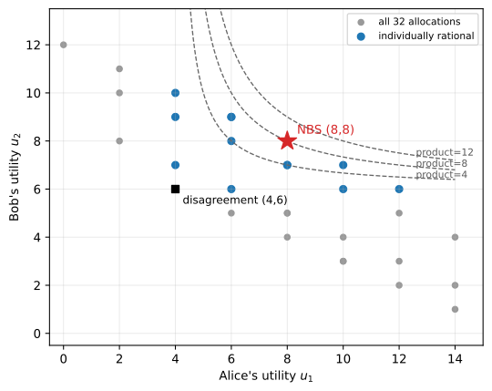
The \(32\) feasible utility pairs for Alice and Bob. The black square is the disagreement point \((4,6)\) where each keeps her own goods; blue points are the \(14\) individually rational allocations. Dashed curves are level sets of the Nash product \((u_1-4)(u_2-6)\). The red star is the Nash bargaining solution \((8,8)\), the feasible point on the highest attainable level set. The surplus-maximizing point \((12,6)\) sits on the zero level set: Bob would gain nothing from it.
Problem 6.5 — Wikipedia articles (open-ended question)
Wikipedia articles (open-ended question).
Take a look at the history pages and the discussion pages of two Wikipedia articles: “Abortion” and “Pythagorean Theorem.” Summarize three key (qualitative) differences you can see between them. (open-ended)
The two articles differ not in how much they are edited but in what makes the argument terminate: “Pythagorean theorem” has an external truth-maker that collapses the editors’ preference profile onto one scale, while “Abortion” has none, so its profile stays high-dimensional and cycle-prone and consensus is manufactured by procedure instead. Three differences, as read from the English Wikipedia histories in late August 2026.
Difference 1 is the ratio of talk to edit, not the volume of edit. The last \(100\) revisions of each article span roughly the same year, and both sit under indefinite semi-protection; what differs by an order of magnitude is the talk page, Talk:Abortion being on its \(53\)rd archive against Talk:Pythagorean theorem’s \(7\)th. Per unit of text changed, the contested article consumes some seven times the deliberation – Section 6.1’s \(n^2\)-versus-\(2^n\) contrast, since similar contributor counts give similar pairwise interaction but vastly more opinion configurations to reconcile.
Difference 2 is disputes over premises versus disputes over presentation. Talk:Pythagorean theorem argues over how to present the history of the result, whether to include the Einstein proof, and manual-of-style conformance: questions of ordering and inclusion among items whose correctness nobody contests, so the disagreement is over the rank list, not the candidates. Talk:Abortion argues over whether particular images may appear at all, whether an advocacy organization counts as a reliable source, and how neutrality applies to contested terminology – arguments about what counts as evidence. That is the split of 6.2: shared premises make conclusion-based aggregation safe, while contested premises force the slower premise-based route, whose outcomes individual editors dislike.
Difference 3 is institutional memory as a cycle-breaker. Talk:Abortion carries a numbered FAQ, with a live 2026 thread revising FAQ item 6; Talk:Pythagorean theorem has no FAQ and needs none. The FAQ is agenda control, not documentation: it removes questions from the ballot so a new arrival cannot restart a settled decision, and without it the same pairwise contests re-run indefinitely with no fixed point. The reverts say the same thing, being justified by pointing at the talk page on one article and ordinary maintenance against citation spam on the other.
The distinguishing claim – that a shared external standard destroys Condorcet cycles – is testable. Let \(N\) editors rank \(M\) rival versions, editor \(i\) scoring version \(j\) as
\[ u_{ij} = \rho \, q_j + \sqrt{1-\rho^2} \, \varepsilon_{ij}, \qquad q_j, \varepsilon_{ij} \sim \mathcal{N}(0,1) \text{ i.i.d.} \]
Here \(q_j\) is verifiable quality, seen identically by everyone, \(\varepsilon_{ij}\) is private taste, and \(\rho\) weights the shared standard: \(\rho = 0\) is impartial culture, \(\rho = 1\) unanimity. Measure the probability that Condorcet voting (Section 6.2.1) admits no winner, the failure mode of Figure 6.2 and of 6.1(b).
import numpy as np, matplotlib.pyplot as plt
rng = np.random.default_rng(6)

def no_condorcet_winner(N, M, rho, trials=4000):
    bad = 0
    for _ in range(trials):
        q = rng.normal(size=M)                      # shared verifiable quality
        e = rng.normal(size=(N, M))                 # private taste
        u = rho*q + np.sqrt(1-rho**2)*e             # editor i's score for version j
        beats = np.zeros((M, M), dtype=int)
        for a in range(M):
            for b in range(M):
                if a != b:
                    beats[a, b] = int(np.sum(u[:, a] > u[:, b]) > N/2)
        if not np.any(beats.sum(axis=1) == M-1):    # no version beats all others
            bad += 1
    return bad/trials

rhos = np.linspace(0, 1, 11)
Ms = [3, 5, 7]
res = {M: [no_condorcet_winner(9, M, r) for r in rhos] for M in Ms}
for M in Ms:
    print("M =", M, " P(no Condorcet winner):", " ".join(f"{p:.3f}" for p in res[M]))

fig, ax = plt.subplots(figsize=(6.4, 4.2))
for M, mk in zip(Ms, ['o', 's', '^']):
    ax.plot(rhos, res[M], marker=mk, label=f'M = {M} candidate versions')
ax.set_xlabel(r'shared-standard weight $\rho$   (0 = pure taste, 1 = pure verifiable quality)')
ax.set_ylabel('P(no Condorcet winner)')
ax.set_title('N = 9 editors ranking M rival versions')
ax.annotate('"Abortion"', (0.05, 0.30), fontsize=10)
ax.annotate('"Pythagorean theorem"', (0.62, 0.06), fontsize=10)
ax.grid(alpha=.3); ax.legend()
plt.savefig('nl-ch06-cycle-probability.svg', dpi=150, bbox_inches='tight')
M = 3  P(no Condorcet winner): 0.073 0.074 0.064 0.053 0.038 0.030 0.016 0.013 0.007 0.003 0.000
M = 5  P(no Condorcet winner): 0.220 0.208 0.183 0.147 0.108 0.077 0.050 0.036 0.019 0.011 0.000
M = 7  P(no Condorcet winner): 0.327 0.303 0.274 0.211 0.169 0.115 0.085 0.052 0.034 0.018 0.000
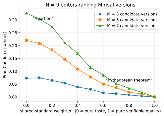
Probability that pairwise majority voting among nine editors admits no Condorcet winner, as a function of how much weight editors place on a shared verifiable standard rather than private taste. Cycles are common when preferences are pure taste and many rival versions are on the table, and vanish once a common yardstick dominates.
With nine editors, seven rival versions and no shared standard, about one dispute in three has no Condorcet winner at all, so there is nothing to converge on; at \(\rho = 0.8\), which is what a verifiability policy buys when the facts are checkable, the failure rate falls to about \(3\%\). The number of rival versions matters as much – at \(\rho = 0\) the cycle rate climbs from \(7\%\) at \(M = 3\) to \(33\%\) at \(M = 7\) – which is why protection is a substantive intervention: it holds \(M\) down.
So the two articles are stable for opposite reasons. On “Pythagorean theorem” the Verifiability policy of Section 6.1 does the work, since a proof either checks out or does not and \(\rho\) is near \(1\). On “Abortion” verifiability cannot collapse the profile, because the dispute is over which verifiable things belong and in what proportion; \(\rho\) stays low and the bargaining apparatus of Section 6.4 substitutes, semi-protection and the FAQ raising the cost of reopening a settled question exactly as raising the disagreement point \(d_i\) does in 6.4.
How do I viralize a YouTube video and tip a Groupon deal?
Problem 7.1 — Perturbing flipping behaviors
Perturbing flipping behaviors.
(a) Consider the influence function \(f(p)\) in Figure 7.13, which has four equilibria \(p^* = 0, \frac{1}{3}, \frac{2}{3}\) and \(1\). Suppose we start with \(p(0) = 0.01\) (or some number slightly greater than 0). Find the equilibrium fraction, denoted as \(p_\infty\).
(b) Suppose \(f(p)\) is slightly modified as in Figure 7.14, such that the point \(p = 0\) is no longer an equilibrium. Again use a graphical argument to find \(p(\infty)\), starting at \(p(0) = 0\).
(c) Suppose \(f(p)\) is further slightly modified as in Figure 7.15, such that \(f(p) > p\) for \(0 \le p < 1\). Find \(p(\infty)\) starting at \(p(0) = 0\).
Figure 7.13 (the “original curve to model flipping”) plots \(f(p)\) against \(p\) on the unit square together with the dashed 45-degree line \(f(p) = p\). The curve leaves the origin steeply, so that it lies strictly above the diagonal on \((0,\tfrac13)\); it flattens through the middle of the range and dips below the diagonal on \((\tfrac13,\tfrac23)\); it then steepens again and lies above the diagonal on \((\tfrac23,1)\), finally flattening to meet the diagonal at \((1,1)\). It therefore touches or crosses the 45-degree line at exactly the four points \(p = 0, \tfrac13, \tfrac23, 1\).
Figure 7.14 is the same curve lifted off the origin: \(f(0) > 0\), so the curve no longer passes through \((0,0)\), but it still crosses the 45-degree line at (approximately) \(\tfrac13\) and \(\tfrac23\) and still ends at \((1,1)\).
Figure 7.15 is the same curve lifted further, so that the middle dip no longer reaches the diagonal: now \(f(p) > p\) for every \(0 \le p < 1\), and \((1,1)\) is the only point of contact with the 45-degree line. (difficulty: \(\star\star\))
\(p_\infty = \tfrac13\) in both (a) and (b), and \(p(\infty) = 1\) in (c).
Under \(p[t+1] = f(p[t])\) of Section 7.2.2 the sign of \(f(p) - p\) gives the direction of motion, and an equilibrium is a barrier the orbit cannot cross. Figure 7.13 has
\begin{equation*} \begin{aligned} f(p) &> p \quad \text{on } (0,\tfrac13), \\ f(p) &< p \quad \text{on } (\tfrac13,\tfrac23), \\ f(p) &> p \quad \text{on } (\tfrac23,1), \end{aligned} \end{equation*}
so arrows point away from \(0\) and from \(\tfrac23\) on both sides (unstable) and towards \(\tfrac13\) and \(1\) (stable). The state space therefore splits at \(\tfrac23\): every point of \((0,\tfrac23)\) flows to \(\tfrac13\), every point of \((\tfrac23,1]\) flows to \(1\).
(a) \(p(0) = 0.01\) lies in \((0,\tfrac13)\), so the orbit increases monotonically, bounded above by \(\tfrac13\), and \(p_\infty = \tfrac13\). One per cent escapes the unstable equilibrium at \(0\) but comes nowhere near the tipping threshold \(\tfrac23\): the clip does not go viral.
(b) \(p(\infty) = \tfrac13\) again. Lifting the curve off the origin removes the equilibrium at \(0\) and nothing else; since the curve is only slightly modified and still crosses the diagonal near \(\tfrac13\), we have \(p(1) = f(0) \in (0,\tfrac13)\) and part (a) applies verbatim. The deleted equilibrium was unstable, so the only orbit it ever attracted was the one sitting exactly on it.
(c) \(p(\infty) = 1\). With \(f(p) > p\) on \([0,1)\) the sole equilibrium is \(p^* = 1\), and from \(p(0) = 0\) the orbit is strictly increasing and bounded above, hence convergent to a fixed point of the continuous map \(f\), necessarily \(1\). Raising the whole curve above the diagonal merges the two attraction regions and deletes the threshold at \(\tfrac23\).
For a numerical check, take \(g(p) = -p(p-\frac13)(p-\frac23)(p-1)\), which has the sign pattern displayed above, so that \(f_a(p) = p + 4g(p)\) reproduces Figure 7.13; a bump supported on \([0,\frac13)\) gives Figure 7.14 and one positive on all of \([0,1)\) gives Figure 7.15.
import numpy as np, matplotlib.pyplot as plt

def g(p):  return -p*(p-1/3)*(p-2/3)*(p-1)
def fa(p): return p + 4.0*g(p)                                  # Figure 7.13
def fb(p): return fa(p) + 0.04*np.maximum(0.0, 1-3*p)**2        # Figure 7.14
def fc(p): return np.minimum(1.0, fa(p) + 0.30*np.sqrt(p)*(1-p)
                                        + 0.05*(1-p)**2)        # Figure 7.15

def orbit(f, p0, n=300):
    p = np.array(float(p0)); seq = [float(p)]
    for _ in range(n):
        p = f(p); seq.append(float(p))
    return seq

grid = np.linspace(0, 1, 2001)
for nm, f in [('f_a', fa), ('f_b', fb), ('f_c', fc)]:
    v = f(grid); d = v[:-1] - grid[:-1]
    print('%s: f(0)=%.3f f(1)=%.3f max=%.3f min(f-p) on [0,1)=%+.5f'
          % (nm, f(np.array(0.)), f(np.array(1.)), v.max(), d.min()))

for nm, f, p0 in [('(a)', fa, 0.01), ('(b)', fb, 0.0), ('(c)', fc, 0.0)]:
    s = orbit(f, p0)
    print(nm, 'p[0..8]=', np.round(s[:9], 4), ' p[300]=%.6f' % s[-1])

fig, axes = plt.subplots(1, 3, figsize=(13, 4.2))
panels = [(fa, 0.01, '(a) Fig. 7.13, p(0)=0.01'),
          (fb, 0.00, '(b) Fig. 7.14, p(0)=0'),
          (fc, 0.00, '(c) Fig. 7.15, p(0)=0')]
for ax, (f, p0, ttl) in zip(axes, panels):
    ax.plot(grid, f(grid), 'k-', lw=1.6, label='f(p)')
    ax.plot(grid, grid, 'k--', lw=1, label='45-degree line')
    x = p0
    for _ in range(25):
        y = f(np.array(x))
        ax.plot([x, x], [x, y], color='C3', lw=.9)
        ax.plot([x, y], [y, y], color='C3', lw=.9)
        x = float(y)
    ax.set_xlim(0, 1); ax.set_ylim(0, 1)
    ax.set_xlabel('p'); ax.set_ylabel('f(p)')
    ax.set_title(ttl, fontsize=10); ax.legend(fontsize=8, loc='upper left')
plt.tight_layout()
plt.savefig('nl-ch07-tipping-cobweb.svg', dpi=150, bbox_inches='tight')
print('figure saved')
f_a: f(0)=0.000 f(1)=1.000 max=1.000 min(f-p) on [0,1)=-0.02778
f_b: f(0)=0.040 f(1)=1.000 max=1.000 min(f-p) on [0,1)=-0.02778
f_c: f(0)=0.050 f(1)=1.000 max=1.000 min(f-p) on [0,1)=+0.00050
(a) p[0..8]= [0.01   0.0184 0.0332 0.0576 0.094  0.1407 0.1897 0.2318 0.2633]  p[300]=0.333333
(b) p[0..8]= [0.     0.04   0.0992 0.1664 0.2228 0.2612 0.2856 0.3013 0.3115]  p[300]=0.333333
(c) p[0..8]= [0.     0.05   0.1921 0.3725 0.4963 0.5877 0.6716 0.7592 0.8538]  p[300]=1.000000
figure saved
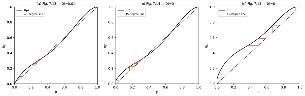
Cobweb diagrams for the three influence functions. Left: Figure 7.13 started at p(0)=0.01 climbs to the stable equilibrium 1/3. Middle: Figure 7.14, with the origin equilibrium removed, starts at 0 and still ends at 1/3. Right: Figure 7.15, with f(p) > p everywhere below 1, walks all the way to full adoption.
Problem 7.2 — Flocking birds
Flocking birds.
In our study of the dynamics of collective behavior, we are often intrigued by the process that turns individual actions and local interactions into large-scale, global patterns. This happens in many ways in human crowds, bird flocks, fish schools, bacteria swarms, etc. A simple and powerful illustration is Conway’s game of life.
Here is a very simple model for bird flocks that assumes away many features but suffices to illustrate the point for a homework problem. Suppose there is a two-dimensional plane with \(N\) points moving in it. Each point has neighbors, which are the points within a circle of radius \(r\) meters. All the points move with the same constant speed, say, 1 unit, but along different directions. At each timeslot, each point’s direction is updated to be the average of its current direction and all the directions of its neighbors. We can think of a graph in which each node is a point, and each link is a neighbor relationship. But this graph evolves over time as the points’ positions change.
Randomly place 100 points in a \(10 \times 10\) units square, and initialize their directions randomly. You should try different values of \(r\). Simulate the above model over time, and describe what happens to the directions of the points.
(For more detail of this model, see T. Vicsek, A. Czirok, E. Ben Jacob, I. Cohen, and O. Schochet, “Novel type of phase transitions in a system of self-driven particles,” Physics Review Letters, vol. 75, pp. 1226-1229, 1995. A comprehensive survey of animal behavior can be found in I. D. Couzin and J. Krause, “Self-organization and collective behavior in vertebrates,” Advances in the Study of Behavior, vol. 32, pp. 1-75, 2003.) (difficulty: \(\star\star\star\))
The directions always align: the noiseless Vicsek model is a consensus algorithm, so \(r\) governs only how fast alignment happens and, when \(r\) is small and the birds move slowly, whether the flock first breaks into sub-flocks that align internally but point different ways.
Angles must be averaged as circular means (\(359^\circ\) and \(1^\circ\) average to \(0^\circ\), not \(180^\circ\)), so with closed neighbourhoods \(\mathcal N_i(t) = \{ j : \|x_j - x_i\| < r\} \cup \{i\}\),
\begin{equation*} \begin{aligned} \theta_i(t+1) &= \arg \sum_{j \in \mathcal N_i(t)} e^{\mathrm i \theta_j(t)}, \\ x_i(t+1) &= x_i(t) + v\big(\cos\theta_i(t+1), \sin\theta_i(t+1)\big), \end{aligned} \end{equation*}
with periodic boundaries on the \(10 \times 10\) square, keeping the density at 1 bird per unit area. Global order is the length of the mean heading vector,
\[ \varphi(t) \;=\; \Big| \frac{1}{N} \sum_{i=1}^{N} e^{\mathrm i \theta_i(t)} \Big| \ \in [0,1], \]
near \(1/\sqrt N \approx 0.1\) for random headings and equal to \(1\) under full alignment.
Alignment is inevitable while the graph keeps connecting: if all directions lie in an arc shorter than \(\pi\), each new direction is the argument of a positive combination of the old unit vectors, hence lies in the cone they span and so in that same arc, strictly inside it unless a bird has no neighbours. The arc width is non-increasing and shrinks whenever a bird sees a different heading. That is the contraction Section 7.4.1 runs for pulse-coupled oscillators, transposed from the time dimension to the direction dimension, and it fails only if the interaction graph splits into components that never touch again, each of which then reaches its own consensus.
Two speed regimes, then: the stated \(v = 1\), a very large step that reshuffles every neighbour set each slot, and Vicsek’s own \(v = 0.05\), in which the graph is quasi-static.
import numpy as np
from scipy.sparse.csgraph import connected_components
from scipy.sparse import csr_matrix

L, N = 10.0, 100

def run(r, V, T, seed):
    rng = np.random.default_rng(seed)
    pos = rng.uniform(0, L, (N, 2))
    th  = rng.uniform(-np.pi, np.pi, N)
    order = np.empty(T); nc = np.empty(T, int)
    for t in range(T):
        order[t] = abs(np.mean(np.exp(1j*th)))
        d = pos[:, None, :] - pos[None, :, :]
        d -= L*np.round(d/L)                       # periodic wrap
        A = (np.hypot(d[:, :, 0], d[:, :, 1]) < r) # closed neighbourhood
        nc[t] = connected_components(csr_matrix(A), directed=False)[0]
        th = np.arctan2(A @ np.sin(th), A @ np.cos(th))   # circular mean
        pos = (pos + V*np.stack([np.cos(th), np.sin(th)], 1)) % L
    return order, nc

def summ(r, V, T=300, reps=10):
    fo = []; tt = []; c0 = []; ce = []
    for sd in range(reps):
        o, nc = run(r, V, T, sd)
        fo.append(o[-1]); c0.append(nc[0]); ce.append(nc[-1])
        w = np.where(o >= 0.99)[0]
        if len(w): tt.append(w[0])
    lab = ('%.0f' % np.mean(tt) if len(tt) == reps
           else '%d/%d runs, med %d' % (len(tt), reps, int(np.median(tt)) if tt else 0))
    return np.mean(c0), np.mean(ce), np.mean(fo), lab

for V, name in [(1.0,  'V = 1.0  (large step: neighbourhoods reshuffle every slot)'),
                (0.05, 'V = 0.05 (small step: the neighbourhood graph is quasi-static)')]:
    print(name)
    for r in [0.5, 0.75, 1.0, 1.5, 2.0, 3.0]:
        c0, ce, fo, lab = summ(r, V)
        print('  r=%.2f  components t=0: %5.1f  t=299: %4.1f   '
              'final order = %.3f   steps to order>=0.99: %s' % (r, c0, ce, fo, lab))
    print()
V = 1.0  (large step: neighbourhoods reshuffle every slot)
  r=0.50  components t=0:  66.7  t=299:  2.8   final order = 0.997   steps to order>=0.99: 9/10 runs, med 86
  r=0.75  components t=0:  38.7  t=299:  1.4   final order = 1.000   steps to order>=0.99: 57
  r=1.00  components t=0:  14.0  t=299:  1.6   final order = 0.992   steps to order>=0.99: 9/10 runs, med 59
  r=1.50  components t=0:   1.0  t=299:  1.2   final order = 0.998   steps to order>=0.99: 9/10 runs, med 27
  r=2.00  components t=0:   1.0  t=299:  1.0   final order = 1.000   steps to order>=0.99: 16
  r=3.00  components t=0:   1.0  t=299:  1.0   final order = 1.000   steps to order>=0.99: 5

V = 0.05 (small step: the neighbourhood graph is quasi-static)
  r=0.50  components t=0:  66.7  t=299:  4.7   final order = 0.808   steps to order>=0.99: 0/10 runs, med 0
  r=0.75  components t=0:  38.7  t=299:  3.1   final order = 0.869   steps to order>=0.99: 2/10 runs, med 245
  r=1.00  components t=0:  14.0  t=299:  1.4   final order = 0.998   steps to order>=0.99: 9/10 runs, med 143
  r=1.50  components t=0:   1.0  t=299:  1.0   final order = 1.000   steps to order>=0.99: 69
  r=2.00  components t=0:   1.0  t=299:  1.0   final order = 1.000   steps to order>=0.99: 22
  r=3.00  components t=0:   1.0  t=299:  1.0   final order = 1.000   steps to order>=0.99: 7
import numpy as np, matplotlib.pyplot as plt

fig, ax = plt.subplots(1, 3, figsize=(14, 4))
for r, st in [(0.5, '-'), (1.0, '--'), (2.0, '-.')]:
    ax[0].plot(run(r, 1.00, 200, 0)[0], st, label='r=%.1f' % r)
    ax[1].plot(run(r, 0.05, 200, 0)[0], st, label='r=%.1f' % r)
ax[0].set_title('V = 1.0 (fast mixing)', fontsize=10)
ax[1].set_title('V = 0.05 (quasi-static graph)', fontsize=10)
for a in ax[:2]:
    a.set_xlabel('timeslot t'); a.set_ylabel('order parameter')
    a.set_ylim(0, 1.05); a.legend(fontsize=8)
rs = np.array([0.4, 0.5, 0.6, 0.75, 0.9, 1.0, 1.25, 1.5, 2.0, 2.5, 3.0])
for V, mk in [(1.0, 'o-'), (0.05, 's-')]:
    ys = [np.mean([run(r, V, 300, sd)[0][-1] for sd in range(6)]) for r in rs]
    ax[2].plot(rs, ys, mk, label='V=%g' % V, ms=4)
ax[2].set_xlabel('neighbourhood radius r'); ax[2].set_ylabel('order at t=300')
ax[2].set_ylim(0, 1.05); ax[2].legend(fontsize=8)
ax[2].set_title('steady-state alignment vs r', fontsize=10)
plt.tight_layout()
plt.savefig('nl-ch07-flocking-order.svg', dpi=150, bbox_inches='tight')
print('figure saved')
figure saved
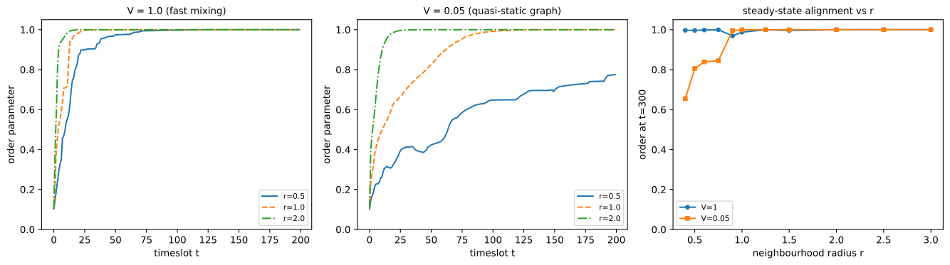
Left and middle: the order parameter over time for three radii, at high and low speed. Right: order at t=300 as a function of r. At speed 1 the flock aligns at every radius tested; at speed 0.05 alignment degrades once r falls below the connectivity radius, which sits near r = 1.
Four things happen to the directions.
They align. The order parameter starts near \(0.1 \approx 1/\sqrt{100}\) and climbs to \(1\), every bird in a component ending on the same heading and the flock translating rigidly. With no noise term there is no disorder to sustain, so unlike the true Vicsek model this version can only order.
Once the graph is connected, \(r\) sets the rate and not the outcome: at \(v = 1\) the time to reach \(\varphi \ge 0.99\) falls from about 86 slots at \(r = 0.5\) to 5 at \(r = 3\), since a denser graph pushes the second eigenvalue of the averaging matrix away from \(1\).
Below the connectivity radius a slow flock fragments. At density 1 the disc graph on 100 points is a single component from about \(r \approx 1.2\) up and has some 67 components at \(r = 0.5\); at \(v = 0.05\) that fragmentation survives, the \(r = 0.5\) runs still showing about 5 components and \(\varphi \approx 0.8\) after 300 slots – several sub-flocks, each internally aligned, merging only occasionally.
Movement is itself a connectivity mechanism. At \(v = 1\) a bird crosses the box in ten slots, so even at \(r = 0.5\) the union of the interaction graphs over a few slots is connected and the contraction applies to that union, giving \(\varphi = 0.997\). Fast sparse-sensing birds flock as well as slow far-sensing ones, and no critical radius appears.
Problem 7.3 — A citation network and matrix multiplication
A citation network and matrix multiplication.
Consider a set of eight papers with their citation relationships represented by the graph in Figure 7.16. Each paper is a node, and a directed edge from node \(i\) to node \(j\) means paper \(i\) cites paper \(j\).
Figure 7.16 is drawn in three ranks. The top rank holds nodes 1 and 2; the middle rank holds 3, 4, 5, 6; the bottom rank holds 7 and 8. The directed edges are
\[ 1 \to 3, \quad 1 \to 4, \quad 2 \to 5, \quad 2 \to 6, \quad 3 \to 7, \quad 4 \to 7, \quad 4 \to 8, \quad 5 \to 7, \quad 5 \to 8, \quad 6 \to 8, \]
so that the two arrows \(4 \to 8\) and \(5 \to 7\) cross in the middle of the picture. Nodes 7 and 8 have no outgoing edges; nodes 1 and 2 have no incoming edges.
(a) Write down the adjacency matrix \(\mathbf A\) (which we will talk much more about in the next chapter), where the \((i,j)\) entry is 1 if node \(i\) points to node \(j\), and 0 otherwise.
(b) Compute the matrix \(\mathbf C\) defined as
\[ \mathbf C = \mathbf A^T \mathbf A, \]
and compare the values \(C_{78}\) and \(C_{75}\). In general, what is the physical interpretation of the entries \(C_{ij}\)?
(c) Now compute
\[ \mathbf A^2 = \mathbf A \mathbf A, \qquad \mathbf A^3 = \mathbf A^2 \mathbf A. \]
Is there anything special about \(\mathbf A^3\)? In general, what do the entries in \(\mathbf A^m\) (where \(m = 1, 2, \ldots\)) represent? (difficulty: \(\star\star\))
(a) Rows are citing papers, columns cited papers:
\begin{equation*} \mathbf A \;=\; \begin{pmatrix} 0&0&1&1&0&0&0&0\\ 0&0&0&0&1&1&0&0\\ 0&0&0&0&0&0&1&0\\ 0&0&0&0&0&0&1&1\\ 0&0&0&0&0&0&1&1\\ 0&0&0&0&0&0&0&1\\ 0&0&0&0&0&0&0&0\\ 0&0&0&0&0&0&0&0 \end{pmatrix}. \end{equation*}
The row sums \((2,2,1,2,2,1,0,0)\) are the out-degrees and the column sums \((0,0,1,1,1,1,3,3)\) the in-degrees, so 7 and 8 are the most cited and cite nobody.
(b) \(C_{78} = 2 > 0 = C_{75}\), and \(\mathbf C = \mathbf A^T \mathbf A\) is the co-citation matrix:
\[ C_{ij} = \sum_{k=1}^{8} A_{ki} A_{kj} = \#\{\,k : k \to i \text{ and } k \to j\,\}, \]
the number of papers citing both \(i\) and \(j\), with \(C_{ii}\) the in-degree of \(i\). This is the citation-network form of the co-visitation count YouTube uses in Section 7.1.1: two papers are related when the same paper cited both. Papers citing 7 are \(\{3,4,5\}\) and papers citing 8 are \(\{4,5,6\}\), so \(C_{78} = |\{4,5\}| = 2\); the only paper citing 5 is 2, which does not cite 7, so \(C_{75} = 0\). Note that 5 cites 7 and yet no co-citation evidence links them: citation is asymmetric, co-citation symmetric, and the two notions of relatedness differ.
(c) \(\mathbf A^3 = \mathbf 0\), and in general
\[ (\mathbf A^m)_{ij} \;=\; \sum_{k_1,\ldots,k_{m-1}} A_{i k_1} A_{k_1 k_2}\cdots A_{k_{m-1} j} \]
counts directed walks of length exactly \(m\) from \(i\) to \(j\), i.e. citation chains of \(m\) hops. Here \(\mathbf A^2\) has four non-zero entries, \((\mathbf A^2)_{17} = 2\) (via 3 and 4), \((\mathbf A^2)_{18} = 1\) (via 4), \((\mathbf A^2)_{27} = 1\) (via 5) and \((\mathbf A^2)_{28} = 2\) (via 5 and 6), while no three-hop chain exists at all: the graph is layered \(\{1,2\} \to \{3,4,5,6\} \to \{7,8\}\) and the bottom layer cites nothing. So \(\mathbf A\) is nilpotent of index 3 with all eigenvalues \(0\), the algebraic signature of a directed acyclic graph – which every citation network is, since one can only cite work that already exists.
import numpy as np

edges = [(1,3),(1,4),(2,5),(2,6),(3,7),(4,7),(4,8),(5,7),(5,8),(6,8)]
A = np.zeros((8,8), int)
for i, j in edges:
    A[i-1, j-1] = 1
print('A =\n', A)
print('out-degrees (references made):', A.sum(1))
print('in-degrees  (citations received):', A.sum(0))

C = A.T @ A
print('C = A^T A =\n', C)
print('C_78 =', C[6,7], '   C_75 =', C[6,4])

A2 = A @ A
A3 = A2 @ A
print('A^2 =\n', A2)
print('A^3 =\n', A3)
print('A^3 is all zero:', not A3.any())
print('eigenvalues of A:', np.round(np.linalg.eigvals(A).real, 12))
A =
 [[0 0 1 1 0 0 0 0]
 [0 0 0 0 1 1 0 0]
 [0 0 0 0 0 0 1 0]
 [0 0 0 0 0 0 1 1]
 [0 0 0 0 0 0 1 1]
 [0 0 0 0 0 0 0 1]
 [0 0 0 0 0 0 0 0]
 [0 0 0 0 0 0 0 0]]
out-degrees (references made): [2 2 1 2 2 1 0 0]
in-degrees  (citations received): [0 0 1 1 1 1 3 3]
C = A^T A =
 [[0 0 0 0 0 0 0 0]
 [0 0 0 0 0 0 0 0]
 [0 0 1 1 0 0 0 0]
 [0 0 1 1 0 0 0 0]
 [0 0 0 0 1 1 0 0]
 [0 0 0 0 1 1 0 0]
 [0 0 0 0 0 0 3 2]
 [0 0 0 0 0 0 2 3]]
C_78 = 2    C_75 = 0
A^2 =
 [[0 0 0 0 0 0 2 1]
 [0 0 0 0 0 0 1 2]
 [0 0 0 0 0 0 0 0]
 [0 0 0 0 0 0 0 0]
 [0 0 0 0 0 0 0 0]
 [0 0 0 0 0 0 0 0]
 [0 0 0 0 0 0 0 0]
 [0 0 0 0 0 0 0 0]]
A^3 =
 [[0 0 0 0 0 0 0 0]
 [0 0 0 0 0 0 0 0]
 [0 0 0 0 0 0 0 0]
 [0 0 0 0 0 0 0 0]
 [0 0 0 0 0 0 0 0]
 [0 0 0 0 0 0 0 0]
 [0 0 0 0 0 0 0 0]
 [0 0 0 0 0 0 0 0]]
A^3 is all zero: True
eigenvalues of A: [0. 0. 0. 0. 0. 0. 0. 0.]
Problem 7.4 — Music in a graph
Music in a graph.
Melodies have been studied as mathematical objects. One way to depict a melody is through a directed graph that visualizes the conditional probabilities of transitions. Following the example in the book Musimathics by G. Loy, we draw the directed graph corresponding to the Oh Susanna chorus, where each node is a diatonic pitch, and each weighted link shows the probability of transition.
Generate a few examples of chorus synthesized by following the transitions shown in the graph in Figure 7.17. See if you can generate something very similar to the original chorus.
You may start to remember random walk on a graph or Markov chain mentioned during our discussion of PageRank in Chapter 3. We can go to a higher order Markov chain by examining the probability of transition into the next note conditioned on the previous and the current notes. It turns out such a second-order Markov chain can quite readily generate a chorus similar to the original one.
Figure 7.17 has seven nodes, the diatonic pitches A through G. Node B is isolated: it carries no links at all. The weighted directed links, printed in the figure as unreduced fractions whose denominator is the number of times the source pitch occurs, are
- from A: \(A \to A\) with \(2/4\), \(A \to G\) with \(2/4\);
- from C: \(C \to D\) with \(3/3\);
- from D: \(D \to C\) with \(2/5\), \(D \to D\) with \(1/5\), \(D \to E\) with \(2/5\);
- from E: \(E \to C\) with \(2/5\), \(E \to D\) with \(1/5\), \(E \to E\) with \(1/5\), \(E \to G\) with \(1/5\);
- from F: \(F \to F\) with \(1/2\), \(F \to A\) with \(1/2\);
- from G: \(G \to A\) with \(1/5\), \(G \to E\) with \(2/5\), \(G \to G\) with \(2/5\).
(difficulty: \(\star\star\))
The original chorus is a \(25\)-note Eulerian trail from \(F\) to \(C\) in the tally multigraph of Figure 7.17, and that is what makes reconstruction possible: Loy’s unreduced fractions (\(2/4\), not \(1/2\)) record a complete transition tally, not merely a stochastic matrix.
As a source each pitch occurs \(A{:}4\), \(C{:}3\), \(D{:}5\), \(E{:}5\), \(F{:}2\), \(G{:}5\), \(B{:}0\), so there are \(24\) transitions and a \(25\)-note melody; as a target, \(A{:}4\), \(C{:}4\), \(D{:}5\), \(E{:}5\), \(F{:}1\), \(G{:}5\). The first note of a trail is the unique node with out-count minus in-count \(= +1\) and the last the unique node with \(-1\), so the chorus starts on \(F\), ends on \(C\) and never uses \(B\) – and Oh! Susanna does have \(25\) syllables.
The graph does not pin the melody down: there are \(25920\) such trails, which is precisely the information a first-order model throws away. Since folk choruses repeat phrases, rank the trails by longest exactly-repeated substring; only eight reach a repeat of eight notes.
import numpy as np, collections

S = ['A','B','C','D','E','F','G']
idx = {s: i for i, s in enumerate(S)}
num = {'A': {'A':2,'G':2},          'C': {'D':3},
       'D': {'C':2,'D':1,'E':2},    'E': {'C':2,'D':1,'E':1,'G':1},
       'F': {'F':1,'A':1},          'G': {'A':1,'E':2,'G':2}}
den = {'A':4, 'C':3, 'D':5, 'E':5, 'F':2, 'G':5}
P = np.zeros((7,7))
for s in num:
    for t, k in num[s].items():
        P[idx[s], idx[t]] = k/den[s]
print('row sums of P:', np.round(P.sum(1), 6))

outc = dict(den)
inc  = collections.Counter()
for s in num:
    for t, k in num[s].items():
        inc[t] += k
print('note counts as source:', outc)
print('note counts as target:', dict(inc))
print('source minus target  :', {s: outc.get(s,0) - inc[s] for s in S})
print('total transitions    :', sum(outc.values()))

edges = collections.Counter()
for s in num:
    for t, k in num[s].items():
        edges[(s,t)] = k
trails = []
def dfs(node, rem, seq):
    if sum(rem.values()) == 0:
        trails.append(''.join(seq)); return
    for t in S:
        if rem.get((node,t), 0) > 0:
            rem[(node,t)] -= 1; seq.append(t)
            dfs(t, rem, seq)
            seq.pop(); rem[(node,t)] += 1
dfs('F', collections.Counter(edges), ['F'])
print('Eulerian trails F -> C:', len(trails), ' each of length', len(trails[0]))

def longest_repeat(p):
    for L in range(10, 3, -1):
        c = collections.Counter(p[i:i+L] for i in range(len(p)-L+1))
        if max(c.values()) > 1:
            return L
    return 0
best = max(longest_repeat(p) for p in trails)
cand = [p for p in trails if longest_repeat(p) == best]
print('longest exactly-repeated phrase over all trails:', best, 'notes;',
      len(cand), 'trails achieve it')
for p in cand:
    print('   ', ' '.join(p))
row sums of P: [1. 0. 1. 1. 1. 1. 1.]
note counts as source: {'A': 4, 'C': 3, 'D': 5, 'E': 5, 'F': 2, 'G': 5}
note counts as target: {'A': 4, 'G': 5, 'D': 5, 'C': 4, 'E': 5, 'F': 1}
source minus target  : {'A': 0, 'B': 0, 'C': -1, 'D': 0, 'E': 0, 'F': 1, 'G': 0}
total transitions    : 24
Eulerian trails F -> C: 25920  each of length 25
longest exactly-repeated phrase over all trails: 8 notes; 8 trails achieve it
    F F A A G G E C D C D D E D E E G A A G G E C D C
    F F A A G G E C D C D D E E D E G A A G G E C D C
    F F A A G G E C D C D E D D E E G A A G G E C D C
    F F A A G G E C D C D E E D D E G A A G G E C D C
    F F A A G G E C D E E G A A G G E C D E D C D D C
    F F A A G G E C D E E G A A G G E C D E D D C D C
    F F A A G G E C D E G A A G G E C D E E D C D D C
    F F A A G G E C D E G A A G G E C D E E D D C D C
Take
\[ \texttt{F F A A G G E C D E} \ \ \big|\ \ \texttt{E G A A G G E C D E D C D D C} \]
as the reconstruction: its repeated phrase \(\texttt{A A G G E C D E}\) sits at notes 3–10 and again at 13–20, and the break at note 10 matches the comma in the lyric (ten syllables, then fifteen). This is a selection under a musical prior, not a derivation – \(25919\) other melodies fit the graph equally well.
Synthesis, and why the first-order chain cannot do it.
orig = 'FFAAGGECDEEGAAGGECDEDCDDC'
print('reconstruction :', ' '.join(orig))
print('repeated phrase:', ' '.join(orig[2:10]), 'at notes 3-10 and again at notes 13-20')

prob = 1.0
for a, b in zip(orig, orig[1:]):
    prob *= P[idx[a], idx[b]]
print('P(this exact 25-note sequence | first-order walk from F) = %.3e = 1 in %.3g'
      % (prob, 1/prob))

rng = np.random.default_rng(7)
def walk1(n=25, start='F'):
    s = start; out = [s]
    for _ in range(n-1):
        s = S[rng.choice(7, p=P[idx[s]])]; out.append(s)
    return ''.join(out)

P2 = collections.defaultdict(collections.Counter)
for a, b, c in zip(orig, orig[1:], orig[2:]):
    P2[(a,b)][c] += 1
def walk2(n=25):
    out = list(orig[:2])
    for _ in range(n-2):
        k = (out[-2], out[-1])
        if k not in P2: break
        o = list(P2[k]); w = np.array([P2[k][x] for x in o], float); w /= w.sum()
        out.append(o[rng.choice(len(o), p=w)])
    return ''.join(out)

print()
print('five first-order syntheses from F:')
for _ in range(5): print('   ', ' '.join(walk1()))
print()
print('five second-order syntheses:')
for _ in range(5): print('   ', ' '.join(walk2()))

def agree(s): return sum(a == b for a, b in zip(s, orig))/len(orig)
N = 20000; ht = collections.Counter(orig)
a1 = []; a2 = []; e1 = e2 = h1 = h2 = 0
for _ in range(N):
    x = walk1(); y = walk2()
    a1.append(agree(x)); a2.append(agree(y))
    e1 += x == orig; e2 += y == orig
    h1 += collections.Counter(x) == ht; h2 += collections.Counter(y) == ht
print()
print('over %d syntheses of 25 notes each:' % N)
print('  1st order: exact %.4f%%  right pitch histogram %5.2f%%  mean note-for-note agreement %.3f'
      % (100*e1/N, 100*h1/N, np.mean(a1)))
print('  2nd order: exact %.4f%%  right pitch histogram %5.2f%%  mean note-for-note agreement %.3f'
      % (100*e2/N, 100*h2/N, np.mean(a2)))

R = [s for s in S if s not in 'BF']
Q = np.array([[P[idx[a], idx[b]] for b in R] for a in R])
w, v = np.linalg.eig(Q.T)
pi = np.real(v[:, np.argmin(abs(w-1))]); pi /= pi.sum()
print('  stationary distribution on the recurrent class {A,C,D,E,G}:',
      {s: round(float(pi[i]), 3) for i, s in enumerate(R)})
reconstruction : F F A A G G E C D E E G A A G G E C D E D C D D C
repeated phrase: A A G G E C D E at notes 3-10 and again at notes 13-20
P(this exact 25-note sequence | first-order walk from F) = 5.243e-10 = 1 in 1.91e+09

five first-order syntheses from F:
    F F F F A A G A G G E C D C D D D E E E G E C D C
    F A G E G G E D C D C D C D C D C D E D E E E C D
    F F F A G A A A A G E G E E E E C D C D C D C D C
    F F F A G G G E C D E D C D E D C D C D E D D C D
    F A A A A G G E D E C D E C D E G A G A G G A A G

five second-order syntheses:
    F F A A G G E C D E E G A A G G E C D E D C D E E
    F F A A G G E C D E D C D E D C D E E G A A G G E
    F F A A G G E C D E E G A A G G E C D E D C D E E
    F F A A G G E C D E E G A A G G E C D D C D E E G
    F F A A G G E C D D C D E D C D E D C D E D C D E

over 20000 syntheses of 25 notes each:
  1st order: exact 0.0000%  right pitch histogram  0.07%  mean note-for-note agreement 0.296
  2nd order: exact 3.4550%  right pitch histogram 22.09%  mean note-for-note agreement 0.609
  stationary distribution on the recurrent class {A,C,D,E,G}: {'A': 0.048, 'C': 0.238, 'D': 0.357, 'E': 0.238, 'G': 0.119}
The first-order syntheses share the pitch set and the local moves – the \(FF\) opening, the \(A \to G\) descent, the \(D \leftrightarrow E\) oscillation – but carry no memory of phrase structure, and they stall in \(\texttt{C D C D C D}\), since \(C \to D\) has probability \(1\) and \(D \to C\) probability \(2/5\). Hitting the original exactly has probability \(5.2 \times 10^{-10}\), and it never occurred in \(20000\) draws.
Conditioning on the previous pair collapses most of the ambiguity, only a handful of contexts then having more than one successor: the exact-match rate rises to \(3.5\%\), note-for-note agreement from \(0.30\) to \(0.61\), and one synthesis in five reproduces the pitch histogram. That is the book’s claim quantified – though a second-order model fitted to a single \(25\)-note example has nearly as many parameters as data points.
Finally, \(F\) is transient (nothing enters it but itself) and \(B\) is isolated, so long-run behaviour lives on \(\{A,C,D,E,G\}\) with \(\pi \approx (0.048, 0.238, 0.357, 0.238, 0.119)\), against the chorus’s own frequencies \((0.16, 0.16, 0.20, 0.20, 0.20)\). A melody is not a sample from its own stationary distribution but a short structured trajectory, which is what first-order models are bad at.
import matplotlib.pyplot as plt

emp = np.zeros(7)
for _ in range(4000):
    for ch in walk1(400):
        emp[idx[ch]] += 1
emp /= emp.sum()

lab = ['A','C','D','E','F','G']
x = np.arange(6); wd = 0.27
fig, ax = plt.subplots(figsize=(7,4))
ax.bar(x-wd, [collections.Counter(orig)[s]/25 for s in lab], wd,
       label='reconstructed chorus (25 notes)')
ax.bar(x,    [np.mean([collections.Counter(walk1())[s] for _ in range(400)])/25
              for s in lab], wd, label='first-order walks of length 25')
ax.bar(x+wd, [emp[idx[s]] for s in lab], wd,
       label='long first-order walk (stationary)')
ax.set_xticks(x); ax.set_xticklabels(lab)
ax.set_xlabel('diatonic pitch'); ax.set_ylabel('frequency')
ax.legend(fontsize=8)
ax.set_title('Pitch frequencies: the chorus vs. what the chain produces', fontsize=10)
plt.tight_layout()
plt.savefig('nl-ch07-susanna-pitches.svg', dpi=150, bbox_inches='tight')
print('figure saved')
figure saved
Pitch frequencies in the reconstructed chorus, in 25-note first-order syntheses, and in the stationary distribution of the chain. Twenty-five-note walks stay close to the chorus’s histogram because they start at F and have not had time to mix; long walks drift to the stationary distribution, which starves A and F and over-weights D.
Problem 7.5 — Networked sampling
Networked sampling.
In sociology, estimating the percentage of a hidden population, e.g., the AIDS-infected population, is difficult. One approach is to start with a few sampled “seeds,” and then ask current sample members to recruit future sample members. The question is how to produce unbiased estimates.
Respondent-driven sampling is a method to address this question, and it is used by many institutions including the US Center for Disease Control and UNAIDS. The basic methodology is random walk on graphs, similar to what we saw in this chapter and in Chapter 2.
(a) First, let us characterize the sampling distribution at equilibrium. Let \(\pi_i\) be the stationary distribution of reaching person \(i\).
Let \(K_{ij}\) be the probability of person \(i\) referring to person \(j\). If each bidirectional link \((i,j)\) has a weight \(w_{(i,j)}\), and the probability of that person \(i\) recruiting person \(j\) is directly proportional to \(w_{(i,j)}\), we have a recruiting mechanism similar to PageRank’s spread of importance scores:
\[ P[i \to j] \;=\; \frac{w_{(i,j)}}{\sum_k w_{(i,k)}} . \]
At equilibrium, what is the probability \(\pi_i\) that person \(i\) has been sampled?
(b) We follow a trajectory of sampling, starting with, say, one person, and running through \(n\) people sampled. If a person \(i\) on the trail of sampling has AIDS, we increment the counter of the infected population by 1. If we simply add these up and divide by \(n\), it gives a biased estimate. The importance-sampling method weights each counter by \(1/(N\pi_i)\). But we often do not know the value of \(N\). So, in respondent-driven sampling, the estimate becomes
\[ (\text{Harmonic mean of } \pi_i) \sum_{\text{infected } i} \frac{1}{\pi_i} . \]
Suppose we have two social groups of equal size, A and B, forming a network, and that the infection rates are \(p_A\) and \(p_B\), respectively. Between groups, links have weights \(c\), where \(c \in (0, 0.5)\). Within each group, links have weights \(1-c\).
If we follow respondent-driven sampling, what do you think will happen to the sampling result? Confirm this with a simulation.
(For more details, see S. Goel and M. Salganik, “Respondent-driven sampling as Markov chain Monte Carlo,” Statistics in Medicine, vol. 28, pp. 2202-2229, 2009.) (difficulty: \(\star\star\star\))
(a) The stationary distribution is proportional to weighted degree: with \(W_i = \sum_k w_{(i,k)}\) person \(i\)’s strength and \(W = \sum_j W_j\),
\[ \pi_i \;=\; \frac{W_i}{W} \;=\; \frac{\sum_k w_{(i,k)}}{\sum_{j,k} w_{(j,k)}} . \]
Detailed balance verifies this: with \(K_{ij} = w_{(i,j)}/W_i\),
\[ \pi_i K_{ij} \;=\; \frac{W_i}{W}\cdot\frac{w_{(i,j)}}{W_i} \;=\; \frac{w_{(i,j)}}{W}, \]
symmetric in \(i\) and \(j\) because the links are bidirectional, so \(\pi_i K_{ij} = \pi_j K_{ji}\); summing over \(j\) gives \(\pi_i = \sum_j \pi_j K_{ji}\), and \(\pi\) is the unique stationary distribution once the graph is connected.
Raw counts are therefore biased towards sociable people, in proportion to their degree. Unlike PageRank’s directed chain in Chapter 3, this one is reversible and \(\pi\) is closed-form in purely local data, so each respondent need report only \(W_i\), and the estimator
\[ \hat p \;=\; \frac{\sum_{\text{infected}} 1/W_i}{\sum_{\text{sample}} 1/W_i} \]
(both sums over the trail) needs neither \(N\) nor \(W\), the normalisation cancelling. This is the printed form: the harmonic mean over the \(n\) sampled people is \(n/\sum_{\text{sample}} 1/\pi_i\), so the printed product equals \(n \hat p\), and dividing by \(n\) leaves \(\hat p\). Self-normalisation is what buys independence from the unknown \(N\).
(b) The result is unbiased in expectation, but its variance explodes as \(c \to 0\).
First, \(\pi\) is uniform here. With groups of size \(h = N/2\), a person in either group has \(h-1\) within-group links of weight \(1-c\) and \(h\) between-group links of weight \(c\), so
\[ W_i \;=\; (h-1)(1-c) + hc \qquad \text{for every } i, \]
(an artefact of the equal group sizes) and \(\pi_i = 1/N\). The degree correction does nothing, the estimator collapses to the plain sample mean \(\#\{\text{infected in the trail}\}/n\), and at equilibrium \(\hat p \to (p_A+p_B)/2\), the true prevalence.
Second, the walk does not reach equilibrium. The chain lumps onto the group label, with per-step crossing probability
\[ q \;=\; \frac{hc}{(h-1)(1-c)+hc} \;\xrightarrow[\ h\ \text{large}\ ]{}\; c . \]
The lumped two-state chain has transition matrix \(\begin{pmatrix} 1-q & q \\ q & 1-q\end{pmatrix}\) with second eigenvalue
\[ \lambda_2 \;=\; 1 - 2q \;\approx\; 1 - 2c, \]
so the relaxation time is \(1/(1-\lambda_2) = 1/(2q) \approx 1/(2c)\) steps: at \(c = 0.01\) the walk needs some fifty referrals merely to forget its starting group, while a real study runs a few chains of a few hundred respondents. Let \(f_b\) be the between-group share of the indicator’s variance,
\[ f_b = \frac{\tfrac12\big[(p_A-\bar p)^2+(p_B-\bar p)^2\big]}{\bar p(1-\bar p)} \]
with \(\bar p = (p_A+p_B)/2\). Draws within a group are independent, so the lag-\(k\) autocorrelation is \(\rho_k = f_b\lambda_2^{\,k}\) and the trail mean carries the Markov-chain design effect
\begin{equation*} \begin{aligned} \mathrm{Var}(\hat p) &= \frac{\bar p(1-\bar p)}{n} \Big[1 + 2\sum_{k=1}^{n-1}\big(1-\tfrac kn\big) f_b \lambda_2^{\,k}\Big] \\ &\xrightarrow[\ n \gg 1/(2q)\ ]{} \ \frac{\bar p(1-\bar p)}{n}\Big[1 + f_b\frac{1-2q}{q}\Big]. \end{aligned} \end{equation*}
The bracket grows like \(f_b/c\), so the prediction is that even seeding keeps the estimate centred while its standard deviation grows like \(1/\sqrt c\), and that at small \(c\) a trail seeded in A returns roughly \(p_A\) and one seeded in B roughly \(p_B\).
Simulating with \(N = 1000\), \(p_A = 0.6\), \(p_B = 0.1\) and \(n = 200\): since all within-group weights agree and all cross-group weights agree, each step is a coin flip of probability \(q\) to change group followed by a uniform draw from the current group, with node identities kept so revisits reuse an infection status.
import numpy as np

N, pA, pB = 1000, 0.6, 0.1
h = N//2
rng0 = np.random.default_rng(0)
status = np.concatenate([rng0.random(h) < pA, rng0.random(h) < pB])
pAr, pBr = status[:h].mean(), status[h:].mean()
p = 0.5*(pAr + pBr)
fb = 0.5*((pAr-p)**2 + (pBr-p)**2) / (p*(1-p))
print('group prevalences realised: A %.4f  B %.4f   overall %.4f' % (pAr, pBr, p))
print('between-group share of variance f_b = %.4f' % fb)

def sim(c, n, reps, seed_group, rng):
    q = (h*c) / ((h-1)*(1-c) + h*c)          # P(a referral crosses groups)
    est = np.empty(reps)
    for r in range(reps):
        g = seed_group if seed_group is not None else rng.integers(2)
        tot = 0
        for t in range(n):
            node = g*h + rng.integers(h)
            tot += status[node]
            if rng.random() < q:
                g = 1-g
        est[r] = tot/n                        # pi is uniform, so RDS = sample mean
    return est, q

def deff_pred(q, n):
    lam = 1 - 2*q
    k = np.arange(1, n)
    return 1 + 2*fb*np.sum((1 - k/n)*lam**k)

rng = np.random.default_rng(1)
n, reps = 200, 4000
iid = np.sqrt(p*(1-p)/n)
print()
print('trail length n = %d, %d trails, seed uniform over the whole population' % (n, reps))
print('   c      q       relax 1/(2q)    mean est    sd est    design effect   predicted')
for c in [0.45, 0.3, 0.2, 0.1, 0.05, 0.02, 0.01]:
    e, q = sim(c, n, reps, None, rng)
    print('  %.2f   %.4f    %8.1f       %.4f     %.4f        %5.2f        %5.2f'
          % (c, q, 1/(2*q), e.mean(), e.std(), (e.std()/iid)**2, deff_pred(q, n)))

print()
print('seed dependence (truth %.4f; group prevalences %.3f and %.3f):' % (p, pAr, pBr))
print('    c       seeded in A          seeded in B')
for c in [0.45, 0.2, 0.05, 0.01, 0.002]:
    eA, q = sim(c, n, reps, 0, rng)
    eB, q = sim(c, n, reps, 1, rng)
    print('  %.3f   %.4f (sd %.4f)   %.4f (sd %.4f)'
          % (c, eA.mean(), eA.std(), eB.mean(), eB.std()))

print()
print('trail length at c = 0.02, seeds uniform:')
for n2 in [50, 200, 1000, 5000]:
    e, q = sim(0.02, n2, 800, None, rng)
    print('  n=%5d   mean est = %.4f   sd %.4f' % (n2, e.mean(), e.std()))
group prevalences realised: A 0.5660  B 0.0840   overall 0.3250
between-group share of variance f_b = 0.2648

trail length n = 200, 4000 trails, seed uniform over the whole population
   c      q       relax 1/(2q)    mean est    sd est    design effect   predicted
  0.45   0.4505         1.1       0.3245     0.0340         1.05         1.06
  0.30   0.3004         1.7       0.3247     0.0379         1.31         1.35
  0.20   0.2003         2.5       0.3257     0.0439         1.76         1.78
  0.10   0.1002         5.0       0.3258     0.0581         3.08         3.06
  0.05   0.0501        10.0       0.3217     0.0787         5.65         5.52
  0.02   0.0200        25.0       0.3282     0.1139        11.83        12.10
  0.01   0.0100        49.9       0.3232     0.1506        20.68        20.55

seed dependence (truth 0.3250; group prevalences 0.566 and 0.084):
    c       seeded in A          seeded in B
  0.450   0.3268 (sd 0.0343)   0.3225 (sd 0.0341)
  0.200   0.3275 (sd 0.0439)   0.3218 (sd 0.0436)
  0.050   0.3376 (sd 0.0762)   0.3120 (sd 0.0770)
  0.010   0.3871 (sd 0.1386)   0.2671 (sd 0.1393)
  0.002   0.4875 (sd 0.1395)   0.1558 (sd 0.1315)

trail length at c = 0.02, seeds uniform:
  n=   50   mean est = 0.3115   sd 0.1907
  n=  200   mean est = 0.3226   sd 0.1189
  n= 1000   mean est = 0.3252   sd 0.0541
  n= 5000   mean est = 0.3253   sd 0.0251
import matplotlib.pyplot as plt

rng = np.random.default_rng(2)
n = 200
cs = np.array([0.45,0.35,0.25,0.2,0.15,0.1,0.07,0.05,0.03,0.02,0.015,0.01])
sd = []; pred = []
iid = np.sqrt(p*(1-p)/n)
for c in cs:
    e, q = sim(c, n, 3000, None, rng)
    sd.append(e.std()); pred.append(iid*np.sqrt(deff_pred(q, n)))

fig, ax = plt.subplots(1, 2, figsize=(11, 4))
ax[0].loglog(cs, sd, 'o', label='simulated sd of RDS estimate')
ax[0].loglog(cs, pred, '-', label='autocorrelation prediction')
ax[0].axhline(iid, ls='--', color='k', lw=1,
              label='sd of an iid sample of the same size')
ax[0].set_xlabel('between-group link weight c')
ax[0].set_ylabel('sd of the estimate (n=200)')
ax[0].legend(fontsize=8)
ax[0].set_title('Precision collapses as the groups separate', fontsize=10)
for c, col in [(0.45, 'C0'), (0.002, 'C3')]:
    eA, _ = sim(c, n, 4000, 0, rng)
    eB, _ = sim(c, n, 4000, 1, rng)
    ax[1].hist(eA, bins=40, alpha=.55, color=col, label='c=%g, seed in A' % c)
    ax[1].hist(eB, bins=40, alpha=.30, color=col, histtype='step', lw=2,
               label='c=%g, seed in B' % c)
ax[1].axvline(p, color='k', ls='--', lw=1, label='true prevalence')
ax[1].set_xlabel('RDS estimate'); ax[1].set_ylabel('count'); ax[1].legend(fontsize=8)
ax[1].set_title('Distribution of the estimate, by seed group', fontsize=10)
plt.tight_layout()
plt.savefig('nl-ch07-rds-variance.svg', dpi=150, bbox_inches='tight')
print('figure saved')
figure saved
Left: the standard deviation of the RDS estimate from a 200-person trail grows like 1/sqrt(c) as the two groups separate, matching the Markov-chain design-effect prediction. Right: with c=0.45 the estimate is tight around the truth regardless of seed; with c=0.002 the seed group all but decides the answer, the two distributions piling up near the two group prevalences 0.57 and 0.08.
Four readings confirm the prediction.
No bias: with uniform seeding every mean estimate sits in \(0.324\)–\(0.328\) against a realised truth of \(0.325\), for all \(c\) from \(0.45\) down to \(0.01\).
Catastrophic variance: the design effect runs \(1.05 \to 20.7\) as \(c\) runs \(0.45 \to 0.01\), so at \(c = 0.01\) two hundred respondents carry the information of about ten independent ones. The autocorrelation formula predicts \(1.06 \to 20.6\), matching to within a few percent, so the mechanism and not just the symptom is confirmed.
Seed dependence is the practical failure mode. At \(c = 0.45\) the seed is irrelevant (\(0.327\) from A against \(0.323\) from B); by \(c = 0.01\) the gap is \(0.387\) against \(0.267\); at \(c = 0.002\), where the relaxation time \(1/(2q) \approx 250\) exceeds the trail length, the seed all but decides the answer, \(0.488\) against \(0.156\) with group prevalences \(0.566\) and \(0.084\). A real study cannot average over seeds as this simulation does.
Longer trails help at the usual \(1/\sqrt n\) rate: at \(c = 0.02\) the standard deviation falls \(0.191 \to 0.119 \to 0.054 \to 0.025\) as \(n\) goes \(50 \to 200 \to 1000 \to 5000\).
So unbiasedness is the wrong reassurance. Usable precision is governed by the spectral gap \(2q \approx 2c\) of the referral chain, and homophily – exactly what makes a hidden population hidden – is what makes that gap small, trapping the sampler in the sub-community it entered. Reported design effects in real RDS studies run from 5 to 10, consistent with \(c \approx 0.03\)–\(0.06\) here.
How do I influence people on Facebook and Twitter?
Problem 8.1 — Computing centrality and betweenness
Computing centrality and betweenness. Figure 8.19 shows a simple undirected graph on five nodes, drawn as a diamond: node \(1\) at the top, node \(2\) at the left corner, node \(3\) in the middle, node \(4\) at the right corner and node \(5\) at the bottom. Its seven links are
\begin{equation*} (1,2),\quad (1,3),\quad (1,4),\quad (2,5),\quad (3,4),\quad (3,5),\quad (4,5). \end{equation*}
(Note in particular that there is no link \((2,3)\) and no link \((2,4)\): node \(2\) touches only nodes \(1\) and \(5\).)
(a) Compute the degree, closeness, and eigenvector centrality of each node in the graph in Figure 8.19.
(b) Compute the node betweenness centrality of nodes \(2\) and \(3\).
(c) Compute the link betweenness centrality of the links \((3,4)\) and \((2,5)\). (difficulty: \(\star\))
Degrees \(3,2,3,3,3\); closeness \(0.8,\ 2/3,\ 0.8,\ 0.8,\ 0.8\); eigenvector centrality \(0.4558,\ 0.3192,\ 0.4912,\ 0.4912,\ 0.4558\); \(B_2 = B_3 = 1/3\); \(B_{(3,4)} = 1\) and \(B_{(2,5)} = 7/3\).
Order the nodes \(1,\dots,5\), so that the adjacency matrix is
\begin{equation*} \mathbf{A}= \begin{bmatrix} 0&1&1&1&0\\ 1&0&0&0&1\\ 1&0&0&1&1\\ 1&0&1&0&1\\ 0&1&1&1&0 \end{bmatrix}. \end{equation*}
Nodes \(1\) and \(5\) share the neighbour set \(\{2,3,4\}\), and \(3 \leftrightarrow 4\) exchanges \(\{1,4,5\}\) with \(\{1,3,5\}\), so both transpositions are automorphisms and every centrality obeys
\begin{equation*} x_1=x_5,\qquad x_3=x_4 . \end{equation*}
(a) Degree, read off the link list:
\begin{equation*} d_1=3,\quad d_2=2,\quad d_3=3,\quad d_4=3,\quad d_5=3 . \end{equation*}
Four of the five nodes already tie at \(3\). For closeness, every pair is at distance \(1\) except
\begin{equation*} d_{15}=2,\qquad d_{23}=2,\qquad d_{24}=2 . \end{equation*}
Applying the definition (8.3), \(C_i=(n-1)/\sum_j d_{ij}\) with \(n=5\):
\begin{equation*} C_1=\frac{4}{1+1+1+2}=\frac{4}{5}=0.8,\qquad C_2=\frac{4}{1+2+2+1}=\frac{4}{6}=0.6667, \end{equation*}
\begin{equation*} C_3=C_4=C_5=\frac{4}{5}=0.8 . \end{equation*}
Only node \(2\) is set apart. For eigenvector centrality, equation (8.2) needs the principal eigenpair of \(\mathbf{A}\); writing \(x_1=x_5=a\), \(x_2=b\), \(x_3=x_4=c\), the three distinct rows of \(\mathbf{A}\mathbf{x}=\lambda_1\mathbf{x}\) are
\begin{equation*} \lambda_1 a=b+2c,\qquad \lambda_1 b=2a,\qquad \lambda_1 c=2a+c . \end{equation*}
The last two give \(b=2a/\lambda_1\) and \(c=2a/(\lambda_1-1)\). Substituting into the first and clearing denominators,
\begin{equation*} \lambda_1^{3}-\lambda_1^{2}-6\lambda_1+2=0 , \end{equation*}
whose largest root is \(\lambda_1=2.8558\). Hence the centrality ratios are fixed exactly by
\begin{equation*} \frac{a}{b}=\frac{\lambda_1}{2}=1.4279,\qquad \frac{c}{b}=\frac{\lambda_1}{\lambda_1-1}=1.5389 . \end{equation*}
Normalising to unit Euclidean length,
\begin{equation*} \mathbf{x}=[\,0.4558\;\; 0.3192\;\; 0.4912\;\; 0.4912\;\; 0.4558\,]^{T}. \end{equation*}
Unlike degree, this separates the ties, ranking \(3=4 > 1=5 > 2\): node \(1\) must spend one of its three links on the weak node \(2\), so its neighbour scores sum to \(1.3016\) against node \(3\)’s \(1.4028\).
(b) Equation (8.4), \(B_i=\sum_{s}\sum_{t<s} n^i_{st}/g_{st}\) over unordered pairs with \(s,t\neq i\). Only the three non-adjacent pairs can contribute:
- \((1,5)\): \(g_{15}=3\), the paths \(1\text{-}2\text{-}5\), \(1\text{-}3\text{-}5\), \(1\text{-}4\text{-}5\);
- \((2,3)\): \(g_{23}=2\), the paths \(2\text{-}1\text{-}3\), \(2\text{-}5\text{-}3\);
- \((2,4)\): \(g_{24}=2\), the paths \(2\text{-}1\text{-}4\), \(2\text{-}5\text{-}4\).
For node \(2\), the pairs \((2,3)\) and \((2,4)\) are excluded because node \(2\) is an endpoint. Only \((1,5)\) remains, and node \(2\) lies on one of its three shortest paths:
\begin{equation*} B_2=\frac{1}{3}. \end{equation*}
For node \(3\), the pair \((2,3)\) is excluded; \((2,4)\) contributes nothing, since neither \(2\text{-}1\text{-}4\) nor \(2\text{-}5\text{-}4\) passes through node \(3\); and \((1,5)\) contributes \(1/3\) via \(1\text{-}3\text{-}5\):
\begin{equation*} B_3=\frac{1}{3}. \end{equation*}
So \(B_2=B_3=1/3\): node \(2\) is last on every other measure yet matches the well-connected node \(3\) here, bridging being a different importance from popularity. The full vector is \(B=[1,\;1/3,\;1/3,\;1/3,\;1]\).
(c) Equation (8.5), \(B_{(i,j)}=\sum_s\sum_{t<s} n^{(i,j)}_{st}/g_{st}\), now summing over all pairs, the link’s own endpoints included.
For link \((3,4)\): the pair \((3,4)\) contributes \(1\) (they are adjacent, the single shortest path is the link). No other pair uses it: the three paths for \((1,5)\) are \(1\text{-}2\text{-}5\), \(1\text{-}3\text{-}5\), \(1\text{-}4\text{-}5\), and the paths for \((2,3)\) and \((2,4)\) route through \(1\) or \(5\). Hence
\begin{equation*} B_{(3,4)}=1 . \end{equation*}
For link \((2,5)\): it carries the pair \((2,5)\) itself (\(1\)), one of the three shortest \(1\!-\!5\) paths (\(1\text{-}2\text{-}5\), contributing \(1/3\)), one of the two shortest \(2\!-\!3\) paths (\(2\text{-}5\text{-}3\), contributing \(1/2\)), and one of the two shortest \(2\!-\!4\) paths (\(2\text{-}5\text{-}4\), contributing \(1/2\)):
\begin{equation*} B_{(2,5)}=1+\frac{1}{3}+\frac{1}{2}+\frac{1}{2}=\frac{7}{3}\approx 2.333 . \end{equation*}
So \(B_{(2,5)}\) is more than twice \(B_{(3,4)}\). Since adjacent nodes have the link itself as their unique shortest path, \(1\) is the floor for any link, and \((3,4)\) attains it: buried in the triangle \(\{3,4,5\}\), every pair that might use it has an equally short route via \(1\) or \(5\). Link \((2,5)\) instead is one of only two ways in or out of node \(2\) – Granovetter’s strength of weak ties, Section 8.2.2.
Verifying (a)–(c) numerically, with the betweenness conventions used above (unordered pairs, endpoints excluded for nodes and included for links, as in the chapter’s worked Figure 8.2):
import numpy as np, networkx as nx, itertools
from fractions import Fraction

G = nx.Graph([(1,2),(1,3),(1,4),(2,5),(3,4),(3,5),(4,5)])
n = G.number_of_nodes()
A = nx.to_numpy_array(G, nodelist=range(1,6))
sp = dict(nx.all_pairs_shortest_path_length(G))
close = {i: (n-1)/sum(sp[i][j] for j in G if j != i) for i in G}
w, V = np.linalg.eigh(A)
x = np.abs(V[:, -1])

print("degree    ", [G.degree(i) for i in range(1,6)])
print("closeness ", [round(close[i],4) for i in range(1,6)])
print("lambda1   = %.4f" % w[-1])
print("eigcent   ", np.round(x,4))
print("cubic root check:", round(w[-1]**3 - w[-1]**2 - 6*w[-1] + 2, 12))

nb = {i: Fraction(0) for i in G}
lb = {frozenset(e): Fraction(0) for e in G.edges()}
for s, t in itertools.combinations(sorted(G), 2):
    P = list(nx.all_shortest_paths(G, s, t)); g = len(P)
    for v in G:
        if v in (s,t): continue
        nb[v] += Fraction(sum(1 for p in P if v in p), g)
    for e in lb:
        k = sum(1 for p in P
                if any(frozenset((p[a],p[a+1])) == e for a in range(len(p)-1)))
        lb[e] += Fraction(k, g)

print("node betweenness", {i: str(nb[i]) for i in sorted(G)})
print("B(3,4) =", lb[frozenset((3,4))], "   B(2,5) =", lb[frozenset((2,5))])
degree     [3, 2, 3, 3, 3]
closeness  [0.8, 0.6667, 0.8, 0.8, 0.8]
lambda1   = 2.8558
eigcent    [0.4558 0.3192 0.4912 0.4912 0.4558]
cubic root check: -0.0
node betweenness {1: '1', 2: '1/3', 3: '1/3', 4: '1/3', 5: '1'}
B(3,4) = 1    B(2,5) = 7/3
Sanity check on the conventions, against Section 8.2.1 and 8.2.2, where the chapter reports \(B_1=12\), \(B_2=2.5\), \(B_{(1,3)}=16\) and \(B_{(1,2)}=7.5\) for the eight-node graph of Figure 8.2:
def betweenness(G):
    nb = {i: Fraction(0) for i in G}
    lb = {frozenset(e): Fraction(0) for e in G.edges()}
    for s, t in itertools.combinations(sorted(G), 2):
        P = list(nx.all_shortest_paths(G, s, t)); g = len(P)
        for v in G:
            if v in (s,t): continue
            nb[v] += Fraction(sum(1 for p in P if v in p), g)
        for e in lb:
            k = sum(1 for p in P
                    if any(frozenset((p[a],p[a+1])) == e for a in range(len(p)-1)))
            lb[e] += Fraction(k, g)
    return nb, lb

F82 = nx.Graph([(1,2),(1,3),(1,4),(2,4),(2,5),(3,6),(3,7),(3,8),(4,5),(6,7),(7,8)])
nb, lb = betweenness(F82)
print("B1 =", nb[1], " B2 =", nb[2], "   book: 12 and 2.5")
print("B(1,3) =", lb[frozenset((1,3))], " B(1,2) =", lb[frozenset((1,2))],
      "  book: 16 and 7.5")
B1 = 12  B2 = 5/2    book: 12 and 2.5
B(1,3) = 16  B(1,2) = 15/2   book: 16 and 7.5
Both match the book, so (b) and (c) are on its own footing.
Problem 8.2 — Contagion
Contagion. Consider the contagion model in the graph in Figure 8.20 with \(p=0.3\). Figure 8.20 is an eight-node graph drawn as two nested squares: the outer square has corners \(1\) (top left), \(2\) (top right), \(8\) (bottom right) and \(7\) (bottom left); the inner square has corners \(3\) (top left), \(4\) (top right), \(6\) (bottom right) and \(5\) (bottom left). Its fourteen links are the four outer sides \((1,2)\), \((2,8)\), \((7,8)\), \((1,7)\); the four inner sides \((3,4)\), \((4,6)\), \((5,6)\), \((3,5)\); the two inner diagonals \((3,6)\) and \((4,5)\); and four spokes joining each outer corner to the nearest inner corner, \((1,3)\), \((2,4)\), \((5,7)\) and \((6,8)\). So the degrees are \(3\) for the four outer nodes \(1,2,7,8\) and \(4\) for the four inner nodes \(3,4,5,6\).
(a) Run the contagion model with node \(1\) initialized at state-1 and the other nodes initialized at state-0.
(b) Run the contagion model with node \(3\) initialized at state-1 and the other nodes initialized at state-0.
(c) Contrast the results from (a) and (b) and explain in terms of the cluster densities of the sets of initially state-0 nodes. (difficulty: \(\star\))
Seeding node \(1\) flips only the outer square \(\{1,2,7,8\}\), in \(2\) rounds; seeding node \(3\) flips all eight nodes in \(4\); the obstruction is the inner square, a cluster of density \(3/4 \ge 1-p\).
By Section 8.2.3 a state-0 node flips irreversibly once a fraction \(p = 0.3\) of its neighbours are state-1, which with only two degrees present is a count: an outer node (degree \(3\), \(1/3 \ge 0.3\)) needs one flipped neighbour, an inner node (degree \(4\), \(1/4 < 0.3 \le 2/4\)) needs two. The inner nodes are the harder ones despite having more neighbours.
(a) Seeding node \(1\):
- \(t=1\): outer nodes \(2\) and \(7\) flip; inner node \(3\) sees \(1/4 < 0.3\) and holds. State-1 \(=\{1,2,7\}\).
- \(t=2\): node \(8\) sees \(2\) and \(7\) and flips; each inner node still sees exactly one flipped neighbour. State-1 \(=\{1,2,7,8\}\).
- \(t=3\): node \(6\) gains node \(8\), still \(1/4\), so nothing flips and the process is at equilibrium.
The outer square flips in \(2\) rounds, the inner square never: four of eight adopt.
(b) Seeding node \(3\):
- \(t=1\): node \(1\) flips; \(4,5,6\) see only node \(3\) and hold. State-1 \(=\{1,3\}\).
- \(t=2\): nodes \(2\) and \(7\) each see node \(1\) and flip. State-1 \(=\{1,2,3,7\}\).
- \(t=3\): node \(4\) sees \(2,3\), node \(5\) sees \(3,7\), node \(8\) sees \(2,7\), and all three flip at \(2/4 \ge 0.3\); node \(6\) still sees only \(3\).
- \(t=4\): node \(6\) sees \(3,4,5,8\) and flips.
Every node is in state-1 after \(4\) rounds.
import networkx as nx, itertools

E = [(1,2),(1,3),(1,7),(2,4),(2,8),(3,4),(3,5),(3,6),
     (4,5),(4,6),(5,6),(5,7),(6,8),(7,8)]
G = nx.Graph(E); p = 0.3

def run(seed):
    S = set(seed); hist = [(0, sorted(S))]; t = 0
    while True:
        t += 1
        new = {v for v in G if v not in S
               if sum(1 for u in G[v] if u in S)/G.degree(v) >= p}
        if not new: break
        S |= new; hist.append((t, sorted(new)))
    return S, hist

for seed in ([1], [3]):
    S, h = run(seed)
    print("seed", seed)
    for t, new in h:
        print("   t=%d flipped %s" % (t, new))
    print("   final state-1:", sorted(S), "  never flip:", sorted(set(G)-S))
seed [1]
   t=0 flipped [1]
   t=1 flipped [2, 7]
   t=2 flipped [8]
   final state-1: [1, 2, 7, 8]   never flip: [3, 4, 5, 6]
seed [3]
   t=0 flipped [3]
   t=1 flipped [1]
   t=2 flipped [2, 7]
   t=3 flipped [4, 5, 8]
   t=4 flipped [6]
   final state-1: [1, 2, 3, 4, 5, 6, 7, 8]   never flip: []
import matplotlib.pyplot as plt

pos = {1:(0,3), 2:(3,3), 3:(1,2), 4:(2,2), 5:(1,1), 6:(2,1), 7:(0,0), 8:(3,0)}

def times(seed):
    S = set(seed); tt = {seed[0]: 0}; t = 0
    while True:
        t += 1
        new = {v for v in G if v not in S
               if sum(1 for u in G[v] if u in S)/G.degree(v) >= p}
        if not new: break
        for v in new: tt[v] = t
        S |= new
    return S, tt

fig, axes = plt.subplots(1, 2, figsize=(11,5))
for ax, seed, lab in zip(axes, ([1],[3]), ['(a) seed node 1', '(b) seed node 3']):
    S, tt = times(seed)
    nx.draw_networkx_edges(G, pos, ax=ax, edge_color='#888888')
    nx.draw_networkx_nodes(G, pos, ax=ax, node_size=900, edgecolors='black',
                           node_color=['#d95f02' if v in S else '#cccccc' for v in G],
                           linewidths=[3 if v in seed else 1 for v in G])
    nx.draw_networkx_labels(G, pos, ax=ax, font_color='white', font_weight='bold',
                            labels={v: (str(tt[v]) if v in tt else '-') for v in G})
    for v in G:
        ax.annotate(str(v), (pos[v][0], pos[v][1]+0.28), ha='center',
                    fontsize=9, color='#333333')
    ax.set_title('%s: %d of 8 flip' % (lab, len(S)))
    ax.axis('off'); ax.set_ylim(-0.5, 3.6)
plt.tight_layout()
plt.savefig('nl-ch08-contagion-seeds.svg', dpi=150, bbox_inches='tight')
print("panels drawn")
panels drawn
Contagion on Figure 8.20 with \(p = 0.3\). Numbers inside nodes are the iteration at which each node flips, a dash means never; the thick outline marks the seed. Left: seeding node 1 stalls after the outer square flips, because the inner square \(\{3,4,5,6\}\) is a cluster of density \(3/4 \ge 1 - p\). Right: seeding node 3 breaks that cluster open and the whole network flips in four rounds.
(c) By the criterion of Section 8.2.3 the network flips completely if and only if the initially state-0 set contains no cluster of density \(1-p = 0.7\) or higher, a cluster of density \(q\) being a set each of whose members has at least a fraction \(q\) of its neighbours inside it.
In (a) the state-0 set \(\{2,3,4,5,6,7,8\}\) contains the inner square, each of whose nodes has three of its four neighbours inside (two inner sides plus a diagonal):
\begin{equation*} \text{density}\big(\{3,4,5,6\}\big)=\min_{i\in\{3,4,5,6\}}\frac{|N(i)\cap\{3,4,5,6\}|}{d_i}=\frac{3}{4}=0.75\ \ge\ 0.7 . \end{equation*}
Each inner node has exactly one link out of the block, so it can never exceed \(1/4 = 0.25 < 0.3\) in state-1: the inner square holds out whatever happens outside, and the cascade dies at four adopters.
In (b) the seed sits inside that block, so the state-0 set is \(\{1,2,4,5,6,7,8\}\), which no longer contains \(\{3,4,5,6\}\), and an exhaustive search over its \(127\) non-empty subsets finds no cluster of density \(0.7\). Taking the whole set as the densest candidate, \(2,7,8\) have all three neighbours inside and \(4,5,6\) three of four, but node \(1\) has only \(2\) of \(3\) (its third neighbour being the seed), so the density, a minimum over members, is \(2/3 < 0.7\); dropping node \(1\) leaves \(2\) and \(7\) at \(2/3\) in turn. With no blocking cluster the criterion guarantees complete flipping.
def clusters(nodes, thr):
    nodes = sorted(nodes); out = []
    for r in range(1, len(nodes)+1):
        for T in itertools.combinations(nodes, r):
            T = set(T)
            if all(sum(1 for u in G[v] if u in T)/G.degree(v) >= thr for v in T):
                out.append(sorted(T))
    return out

for seed in ([1], [3]):
    z = sorted(set(G) - set(seed))
    c = clusters(z, 1-p)
    print("initially state-0:", z)
    print("   clusters of density >= 0.7:", c if c else "NONE")
print("density of {3,4,5,6}:",
      {v: "%d/%d" % (sum(1 for u in G[v] if u in {3,4,5,6}), G.degree(v))
       for v in [3,4,5,6]})
initially state-0: [2, 3, 4, 5, 6, 7, 8]
   clusters of density >= 0.7: [[3, 4, 5, 6]]
initially state-0: [1, 2, 4, 5, 6, 7, 8]
   clusters of density >= 0.7: NONE
density of {3,4,5,6}: {3: '3/4', 4: '3/4', 5: '3/4', 6: '3/4'}
What wins for node \(3\) is membership rather than degree: seeding inside the tight cluster deletes it from the state-0 set, removing the graph’s only obstruction.
Problem 8.3 — SIRS infection model
SIRS infection model. We consider an extension to the SIR model that allows nodes in state R to go to state S. This model, known as the SIRS model, accounts for the possibility that a person loses the acquired immunity over time.
Consider the state diagram in Figure 8.21: the same chain as the SIR model of Figure 8.5, \(S \xrightarrow{\ \beta\ } I \xrightarrow{\ \gamma\ } R\), plus one extra arc \(R \xrightarrow{\ \nu\ } S\) carrying the recovered back to susceptible. We can write out the set of differential equations as
\begin{equation*} \frac{dS(t)}{dt}=-\beta S(t)I(t)+\nu R(t), \end{equation*}
\begin{equation*} \frac{dI(t)}{dt}=\beta S(t)I(t)-\gamma I(t), \end{equation*}
\begin{equation*} \frac{dR(t)}{dt}=\gamma I(t)-\nu R(t). \end{equation*}
Modify the Matlab code www.network20q.com/hw/simulate_SIR.m for the numerical solution of the SIR model. Solve for \(t=1,2,\dots,200\) (set the tspan vector in code accordingly) with the following parameters and initial conditions: \(\beta=1\), \(\gamma=1/3\), \(\nu=1/50\), \(I(0)=0.1\), \(S(0)=0.9\), and \(R(0)=0\). Describe and explain your observations. (difficulty: \(\star\star\))
The single arc \(R \to S\) destroys the SIR conclusion that everyone ends up recovered: the disease becomes endemic, the trajectory oscillating in damped waves about
\begin{equation*} S^*=\frac13=0.3333,\qquad I^*=\frac{2}{53}=0.03774,\qquad R^*=\frac{100}{159}=0.62893 . \end{equation*}
An initial outbreak is forced, since \(\sigma=\beta/\gamma=3\) gives \(\sigma S(0)=2.7>1\) (Section 8.2.4). For the equilibrium, \(dI/dt=0\) with \(I^*\ne 0\) forces \(\beta S^*=\gamma\), so \(S^*=1/\sigma=1/3\) whatever \(\nu\) and the initial condition are – the susceptible fraction is pinned at the invasion threshold. Then \(dR/dt=0\) gives \(R^*=\gamma I^*/\nu=\tfrac{50}{3}I^*\), and \(S^*+I^*+R^*=1\) gives \(I^*\tfrac{53}{3}=\tfrac23\), whence the values above: a permanent \(3.8\%\) prevalence.
To see how it is approached, linearise, eliminating \(R=1-S-I\):
\begin{equation*} \dot S=-\beta SI+\nu(1-S-I),\qquad \dot I=\beta SI-\gamma I . \end{equation*}
The Jacobian at \((S^*,I^*)\) is
\begin{equation*} J=\begin{bmatrix}-\beta I^*-\nu & -\beta S^*-\nu\\[2pt] \beta I^* & \beta S^*-\gamma\end{bmatrix} =\begin{bmatrix}-0.05774 & -0.35333\\ 0.03774 & 0\end{bmatrix}, \end{equation*}
using \(\beta S^*-\gamma=0\). Trace \(-\beta I^*-\nu=-0.05774<0\), determinant \(\beta I^*(\beta S^*+\nu)=0.01333>0\) and discriminant \(\mathrm{tr}^2-4\det<0\), so the eigenvalues are the conjugate pair
\begin{equation*} \lambda_{\pm}=-0.02887\pm 0.11180\,i , \end{equation*}
predicting damped oscillation with decay time \(1/0.02887=34.6\) and period \(2\pi/0.1118=56.2\), hence about three and a half waves over \(t\in[0,200]\).
Integrating with solve_ivp (the stand-in for the book’s ode45 script) on \(t = 1,2,\dots,200\):
import numpy as np
from scipy.integrate import solve_ivp

beta, gamma, nu = 1.0, 1/3, 1/50

def sirs(t, y):
    S, I, R = y
    return [-beta*S*I + nu*R, beta*S*I - gamma*I, gamma*I - nu*R]

t_eval = np.arange(0, 201, 1.0)
sol = solve_ivp(sirs, [0, 200], [0.9, 0.1, 0.0],
                t_eval=t_eval, rtol=1e-10, atol=1e-12)
S, I, R = sol.y

Sst = gamma/beta
Ist = nu*(1-Sst)/(gamma+nu)
Rst = gamma*Ist/nu
print("sigma = beta/gamma = %.4f ,  sigma*S(0) = %.4f" % (beta/gamma, beta/gamma*0.9))
print("endemic equilibrium  S*=%.4f  I*=%.4f  R*=%.4f  (sum %.4f)"
      % (Sst, Ist, Rst, Sst+Ist+Rst))
peaks = [k for k in range(1, len(I)-1) if I[k] > I[k-1] and I[k] >= I[k+1]]
print("local maxima of I at t =", [int(t_eval[k]) for k in peaks],
      " with I =", np.round(I[peaks], 4))
print("t=200 :  S=%.4f  I=%.4f  R=%.4f" % (S[-1], I[-1], R[-1]))

J = np.array([[-beta*Ist-nu, -beta*Sst-nu], [beta*Ist, beta*Sst-gamma]])
ev = np.linalg.eigvals(J)
print("Jacobian eigenvalues:", np.round(ev, 5))
print("decay time 1/|Re| = %.2f ,  period 2pi/Im = %.2f"
      % (1/abs(ev[0].real), 2*np.pi/abs(ev[0].imag)))
sigma = beta/gamma = 3.0000 ,  sigma*S(0) = 2.7000
endemic equilibrium  S*=0.3333  I*=0.0377  R*=0.6289  (sum 1.0000)
local maxima of I at t = [4, 63, 119, 175]  with I = [0.338  0.0605 0.0416 0.0385]
t=200 :  S=0.3329  I=0.0374  R=0.6296
Jacobian eigenvalues: [-0.02887+0.1118j -0.02887-0.1118j]
decay time 1/|Re| = 34.64 ,  period 2pi/Im = 56.20
import matplotlib.pyplot as plt

def rhs(t, y, n):
    S, I, R = y
    return [-beta*S*I + n*R, beta*S*I - gamma*I, gamma*I - n*R]

a = solve_ivp(rhs, [0,200], [0.9,0.1,0.0], t_eval=t_eval, args=(nu,),
              rtol=1e-10, atol=1e-12)
b = solve_ivp(rhs, [0,200], [0.9,0.1,0.0], t_eval=t_eval, args=(0.0,),
              rtol=1e-10, atol=1e-12)

fig, ax = plt.subplots(1, 2, figsize=(12,4.4), sharey=True)
for k, (A, ttl) in enumerate([(a, 'SIRS,  nu = 1/50'), (b, 'SIR,  nu = 0')]):
    ax[k].plot(t_eval, A.y[0], label='S(t)', lw=2, color='#1b6ca8')
    ax[k].plot(t_eval, A.y[1], label='I(t)', lw=2, color='#d1495b')
    ax[k].plot(t_eval, A.y[2], label='R(t)', lw=2, color='#3f8f5f')
    ax[k].set_title(ttl); ax[k].set_xlabel('t'); ax[k].grid(alpha=.3)
for y, c in ((Sst,'#1b6ca8'), (Ist,'#d1495b'), (Rst,'#3f8f5f')):
    ax[0].axhline(y, ls=':', color=c, lw=1.2)
ax[0].set_ylabel('population fraction'); ax[0].legend(loc='center right')
ax[0].annotate('endemic equilibrium (dotted)', (88, 0.72), fontsize=9, color='#555555')
plt.tight_layout()
plt.savefig('nl-ch08-sirs.svg', dpi=150, bbox_inches='tight')
print("SIR (nu=0) at t=200:  S=%.4f  I=%.2e  R=%.4f"
      % (b.y[0,-1], b.y[1,-1], b.y[2,-1]))
SIR (nu=0) at t=200: S=0.0524 I=5.36e-13 R=0.9476
SIRS with \(\beta=1\), \(\gamma=1/3\), \(\nu=1/50\) (left) against the same run with \(\nu=0\), i.e. the plain SIR model of Section 8.2.4 (right). Dotted lines on the left mark the endemic equilibrium \(S^*=1/3\), \(I^*=2/53\), \(R^*=100/159\). Losing immunity converts a one-shot epidemic into damped waves around a permanent endemic level.
Four observations.
An outbreak first, as in SIR: \(I\) rises from \(0.1\) to a peak \(0.338\) at \(t=4\) while \(S\) crashes from \(0.9\) to about \(0.12\), growth stopping exactly as \(S\) falls through \(1/\sigma = 1/3\), where \(\beta S = \gamma\).
The epidemic then recurs. At \(\nu=0\) the story would end with \(I \to 0\) and \((S,R)\) frozen at \((0.0524, 0.9476)\); with \(\nu = 1/50\) the \(R\) pool leaks back at rate \(\nu R\), \(S\) climbs past \(1/3\) near \(t \approx 30\), and smaller epidemics fire: \(I = 0.0605\) at \(t=63\), \(0.0416\) at \(t=119\), \(0.0385\) at \(t=175\).
The waves are damped at the predicted period: inter-peak spacings \(59, 56, 56\) against the linearised \(56.2\), and peak heights \(0.338 \to 0.0605 \to 0.0416 \to 0.0385\) decaying to \(I^* = 0.0377\) consistently with the decay time \(34.6\).
The limit is endemic: at \(t = 200\) the solver gives \((0.3329, 0.0374, 0.6296)\) against the analytic \((0.3333, 0.0377, 0.6289)\).
The ringing is overshoot in a slow negative-feedback loop. Infection and recovery run on timescale \(1/\gamma = 3\) while immunity loss runs on \(1/\nu = 50\), so the outbreak consumes susceptibles far past \(S = 1/3\) before the stock of infectives drains; only the slow \(\nu R\) drip restores \(S\), by which time \(I\) is tiny, so \(S\) overshoots upward before the next outbreak catches it – which is what the complex eigenvalue pair encodes.
Problem 8.4 — Information centrality
Information centrality. Consider a weighted, undirected, and connected graph with \(N\) nodes, where the weight for link \((i,j)\) is \(x_{ij}\). First construct a matrix \(\mathbf{A}\) where the diagonal entries \(A_{ii}=1+\sum_j x_{ij}\), \(A_{ij}=1-x_{ij}\) if nodes \(i\) and \(j\) are adjacent, and \(A_{ij}=1\) otherwise.
Now compute the inverse: \(\mathbf{C}=\mathbf{A}^{-1}\). The following quantity is called the information centrality of node \(i\):
\begin{equation*} C_I(i)=\frac{1}{C_{ii}+(T-2R)/N}, \end{equation*}
where \(T=\sum_i C_{ii}\) is the trace of matrix \(\mathbf{C}\) and \(R=\sum_j C_{ij}\) is (any) row sum of matrix \(\mathbf{C}\).
Can you think of why this metric is called information centrality? (difficulty: \(\star\star\))
\(C_I(i)\) is closeness centrality (8.3) with the hop distance replaced by the effective electrical resistance \(\Omega_{ij}\) of the network in which link \((i,j)\) is a resistor of conductance \(x_{ij}\):
\begin{equation*} C_I(i)=\frac{N}{\sum_j \Omega_{ij}} . \end{equation*}
The name is literal because \(1/\Omega_{ij}\) is the information \(i\) can exchange with \(j\) when every path carries a share – informations, like conductances, add in parallel – and \(C_I(i)\) is, up to the constant \(N/(N-1)\), the harmonic mean of those amounts. This is Stephenson and Zelen’s measure, the “count all paths, not just the shortest” repair of (8.3), (8.4) and (8.5).
Write \(\mathbf{L}\) for the weighted Laplacian, \(L_{ii}=\sum_j x_{ij}\) and \(L_{ij}=-x_{ij}\) for \(i \ne j\) (with \(x_{ij}=0\) for non-adjacent pairs), and \(\mathbf{J}=\mathbf{1}\mathbf{1}^T\). Entry by entry,
\begin{equation*} A_{ii}=1+\textstyle\sum_j x_{ij}=L_{ii}+1,\qquad A_{ij}=1-x_{ij}=L_{ij}+1 \ \ (i\sim j),\qquad A_{ij}=1=0+1 \ \ (i\not\sim j), \end{equation*}
so
\begin{equation*} \mathbf{A}=\mathbf{L}+\mathbf{J},\qquad \mathbf{C}=(\mathbf{L}+\mathbf{J})^{-1}. \end{equation*}
The \(+\mathbf{J}\) is the grounded-Laplacian trick: \(\mathbf{L}\mathbf{1}=\mathbf{0}\) is singular, and adding \(\mathbf{J}\) lifts exactly the null direction \(\mathbf{1}\) (as \(\mathbf{J}\mathbf{1}=N\mathbf{1}\)) while leaving \(\mathbf{1}^{\perp}\) untouched, so \(\mathbf{A}\) is invertible on any connected graph. From \((\mathbf{L}+\mathbf{J})\mathbf{1}=N\mathbf{1}\) we get \(\mathbf{C}\mathbf{1}=\tfrac1N\mathbf{1}\): every row of \(\mathbf{C}\) sums to \(R=1/N\), which is why the problem may say “(any) row sum”.
For the key identity, fix \(i\ne j\) and set \(\mathbf{b}=\mathbf{e}_i-\mathbf{e}_j\), the vector that injects one unit of current at \(i\) and draws it out at \(j\). Because \(\mathbf{1}^T\mathbf{b}=0\) we have \(\mathbf{J}\mathbf{b}=\mathbf{0}\). Let \(\mathbf{v}=\mathbf{C}\mathbf{b}\), so \((\mathbf{L}+\mathbf{J})\mathbf{v}=\mathbf{b}\), i.e. \(\mathbf{L}\mathbf{v}+(\mathbf{1}^T\mathbf{v})\mathbf{1}=\mathbf{b}\). Premultiplying by \(\mathbf{1}^T\) and using \(\mathbf{1}^T\mathbf{L}=\mathbf{0}^T\) gives \(N\,\mathbf{1}^T\mathbf{v}=0\), hence \(\mathbf{1}^T\mathbf{v}=0\) and
\begin{equation*} \mathbf{L}\mathbf{v}=\mathbf{b}. \end{equation*}
So \(\mathbf{v}\) is exactly the vector of node voltages produced by injecting one amp at \(i\) and extracting it at \(j\) (Kirchhoff’s current law is \(\mathbf{L}\mathbf{v}=\mathbf{b}\)). The voltage drop across the terminals is the effective resistance:
\begin{equation*} \Omega_{ij}=v_i-v_j=\mathbf{b}^T\mathbf{v}=\mathbf{b}^T\mathbf{C}\mathbf{b}=C_{ii}+C_{jj}-2C_{ij}. \end{equation*}
Summing over \(j\), the \(j=i\) term being \(0\), with \(\sum_j C_{jj}=T\) and \(\sum_j C_{ij}=R\):
\begin{equation*} \sum_j \Omega_{ij}=N\,C_{ii}+T-2R . \end{equation*}
Therefore
\begin{equation*} C_I(i)=\frac{1}{C_{ii}+(T-2R)/N}=\frac{N}{N C_{ii}+T-2R}=\frac{N}{\sum_j \Omega_{ij}} . \end{equation*}
Against equation (8.3), \(C_i=(n-1)/\sum_j d_{ij}\), this is the same object with resistance in place of hop count and a cosmetic \(N\) for \(N-1\), which never affects rankings.
The “information” reading is statistical rather than electrical. A long path is a noisy channel: model the signal received over a path as having variance proportional to its length, so the information it delivers is the reciprocal of that length, and independent paths used at once contribute additively. Adding reciprocal lengths in parallel is the rule for conductances in parallel, so the information flowing between \(i\) and \(j\) over the whole tangle of paths is the effective conductance
\begin{equation*} I_{ij}=\frac{1}{\Omega_{ij}} . \end{equation*}
and the information centrality of \(i\) is the harmonic mean of \(\{I_{ij}\}_{j\ne i}\):
\begin{equation*} \Big[\frac{1}{N-1}\sum_{j\ne i}\frac{1}{I_{ij}}\Big]^{-1}=\frac{N-1}{\sum_j \Omega_{ij}}=\frac{N-1}{N}\,C_I(i). \end{equation*}
So \(C_I(i)\) is how much information \(i\) can exchange with the rest of the network on average; modern texts call the same quantity current-flow closeness centrality.
The measure is genuinely different because (8.3), (8.4) and (8.5) discard every non-shortest path while this one keeps all of them, weighted down by length. Two consequences follow. By Rayleigh monotonicity, adding or strengthening any link lowers every \(\Omega_{ij}\) and so raises every \(C_I\), strictly at the changed link’s endpoints, even when no shortest path shortens by a hop; and where many nodes share a hop profile, closeness ties them while information centrality separates them by redundancy. Verifying the algebra and both consequences:
import numpy as np, networkx as nx

rng = np.random.default_rng(7)
G = nx.Graph([(0,1),(0,2),(1,2),(2,3),(3,4),(3,5),(4,5),(1,4)])
for u, v in G.edges():
    G[u][v]['x'] = round(float(rng.uniform(0.5, 2.0)), 3)
N = G.number_of_nodes()

X = nx.to_numpy_array(G, weight='x')
A = np.where(X > 0, 1 - X, 1.0)
np.fill_diagonal(A, 1 + X.sum(axis=1))
L = np.diag(X.sum(axis=1)) - X
print("A equals Laplacian + all-ones?", np.allclose(A, L + np.ones((N,N))))

C = np.linalg.inv(A)
T = np.trace(C); Rrow = C.sum(axis=1)
print("row sums of C:", np.round(Rrow, 6), "-> all equal 1/N =", round(1/N, 6))
CI = 1.0/(np.diag(C) + (T - 2*Rrow[0])/N)

Lp = np.linalg.pinv(L)
Om = np.array([[Lp[i,i] + Lp[j,j] - 2*Lp[i,j] for j in range(N)] for i in range(N)])
OmC = np.array([[C[i,i] + C[j,j] - 2*C[i,j] for j in range(N)] for i in range(N)])
print("C gives the true effective resistances?", np.allclose(Om, OmC))
print("C_I from the book formula:", np.round(CI, 6))
print("N / sum_j Omega_ij       :", np.round(N/Om.sum(axis=1), 6))

close = np.array([(N-1)/sum(nx.shortest_path_length(G, i, j) for j in G if j != i)
                  for i in range(N)])
print("hop closeness (8.3)      :", np.round(close, 4))
A equals Laplacian + all-ones? True
row sums of C: [0.166667 0.166667 0.166667 0.166667 0.166667 0.166667] -> all equal 1/N = 0.166667
C gives the true effective resistances? True
C_I from the book formula: [1.478468 1.766234 1.801432 1.723058 1.796697 1.263223]
N / sum_j Omega_ij       : [1.478468 1.766234 1.801432 1.723058 1.796697 1.263223]
hop closeness (8.3)      : [0.5556 0.7143 0.7143 0.7143 0.7143 0.5556]
Closeness gives four of the six nodes the identical score \(0.7143\); information centrality separates them into \(1.766\), \(1.801\), \(1.723\), \(1.797\), ranking node \(2\) first because its routes to the rest of the graph are the most redundant.
The second consequence, that strengthening a tie raises centrality without moving any hop distance:
def info_centrality(G, weight='x'):
    N = G.number_of_nodes()
    X = nx.to_numpy_array(G, weight=weight)
    A = np.where(X > 0, 1 - X, 1.0)
    np.fill_diagonal(A, 1 + X.sum(axis=1))
    C = np.linalg.inv(A)
    return 1.0/(np.diag(C) + (np.trace(C) - 2*C.sum(axis=1)[0])/N)

H = nx.Graph(); H.add_edges_from([(0,1),(1,2),(2,3),(3,0),(0,2)], x=1.0)
H2 = H.copy(); H2[0][2]['x'] = 5.0     # strengthen the 0-2 tie only
print("hop distances unchanged:",
      nx.floyd_warshall_numpy(H).tolist() == nx.floyd_warshall_numpy(H2).tolist())
print("C_I, all weights 1:", np.round(info_centrality(H), 4))
print("C_I, x_02 = 5     :", np.round(info_centrality(H2), 4))
hop distances unchanged: True
C_I, all weights 1: [2.2857 1.7778 2.2857 1.7778]
C_I, x_02 = 5     : [3.2  1.92 3.2  1.92]
Every hop distance is identical across the two graphs, so closeness and both betweennesses are unchanged, yet every \(C_I\) rises and the strengthened link’s endpoints rise most (\(2.286\to3.200\) against \(1.778\to1.920\)): tie strength is invisible to the shortest-path measures and visible to this one.
Problem 8.5 — Hypergraphs and bipartite graphs
Hypergraphs and bipartite graphs. Why must a link be defined as the connection between just two nodes? Suppose eight papers are in the fields of physics or chemistry. Group membership, i.e., to which field a paper belongs, is presented as a hypergraph in Figure 8.22. Each dotted area is a group or a hyperedge, which is a generalization of an undirected edge to connect possibly more than two nodes. Papers 4 and 5 are “interdisciplinary” papers, so their nodes are contained in both hyperedges.
Figure 8.22 draws two overlapping dotted lobes meeting in the middle, like a figure eight lying on its side. The left lobe is labelled Physics and encloses nodes \(1\), \(3\), \(7\) together with the two nodes \(4\) and \(5\) in the overlap; the right lobe is labelled Chemistry and encloses nodes \(2\), \(6\), \(8\) together with the same \(4\) and \(5\). So the two hyperedges are
\begin{equation*} h_{\text{Physics}}=\{1,3,4,5,7\},\qquad h_{\text{Chemistry}}=\{2,4,5,6,8\}. \end{equation*}
(a) We can transform the hypergraph in Figure 8.22 into an undirected bipartite graph by introducing two more nodes, each representing one of the hyperedges, and linking a “standard” node to a “hyperedge” node if the former is contained in the corresponding hyperedge. Draw this bipartite graph.
(b) Define an incidence matrix \(\mathbf{B}\) of size \(2\times 8\) with
\begin{equation*} B_{ij}=\begin{cases}1 & \text{node } j \text{ is contained in group } i,\\ 0 & \text{otherwise,}\end{cases} \end{equation*}
where group 1 is “Physics” and group 2 is “Chemistry.” Write down \(\mathbf{B}\) for this graph.
(c) Compute the matrix \(\mathbf{B}^T\mathbf{B}\). What is its interpretation?
(d) Compute the matrix \(\mathbf{B}\mathbf{B}^T\). What is its interpretation? (difficulty: \(\star\star\))
(a) Promote the hyperedges to nodes \(P\) and \(C\), giving node set \(\{1,\dots,8\}\cup\{P,C\}\) and ten links, one per membership:
\begin{equation*} (P,1),\ (P,3),\ (P,4),\ (P,5),\ (P,7),\qquad (C,2),\ (C,4),\ (C,5),\ (C,6),\ (C,8). \end{equation*}
Every link joins a paper to a field, so the graph is bipartite with parts \(\{1,\dots,8\}\) and \(\{P,C\}\), and papers \(4\) and \(5\), the only degree-\(2\) paper nodes, are what keeps it connected. The encoding is faithful: the hypergraph reads straight back off it, and every tool of Section 8.2 now applies.
import networkx as nx
import matplotlib.pyplot as plt

groups = {'Physics': [1,3,4,5,7], 'Chemistry': [2,4,5,6,8]}
G = nx.Graph()
for g, mem in groups.items():
    for j in mem:
        G.add_edge(g, j)

pos = {j: (j-1, 0) for j in range(1, 9)}
pos['Physics'] = (1.5, 2); pos['Chemistry'] = (5.5, 2)
fig, ax = plt.subplots(figsize=(9, 3.6))
nx.draw_networkx_edges(G, pos, ax=ax, edge_color='#999999')
nx.draw_networkx_nodes(G, pos, nodelist=list(range(1,9)), node_color='#eeeeee',
                       edgecolors='black', node_size=650, ax=ax)
nx.draw_networkx_nodes(G, pos, nodelist=['Physics','Chemistry'], node_color='#d95f02',
                       edgecolors='black', node_size=4200, node_shape='s', ax=ax)
nx.draw_networkx_labels(G, pos, labels={j: str(j) for j in range(1,9)}, ax=ax)
nx.draw_networkx_labels(G, pos, labels={'Physics':'Physics','Chemistry':'Chemistry'},
                        ax=ax, font_color='white', font_size=8, font_weight='bold')
ax.set_ylim(-0.6, 2.6); ax.axis('off'); plt.tight_layout()
plt.savefig('nl-ch08-bipartite.svg', dpi=150, bbox_inches='tight')
print("bipartite: %d nodes, %d links" % (G.number_of_nodes(), G.number_of_edges()))
bipartite: 10 nodes, 10 links
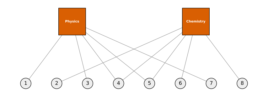
The hypergraph of Figure 8.22 redrawn as a bipartite graph. Each dotted lobe becomes a square hyperedge node; a paper links to a field node when it belongs to that field. The interdisciplinary papers 4 and 5 are the only ones with degree 2, and they are what keeps the graph connected.
(b) With columns indexed \(1\) through \(8\),
\begin{equation*} \mathbf{B}= \begin{bmatrix} 1&0&1&1&1&0&1&0\\ 0&1&0&1&1&1&0&1 \end{bmatrix}. \end{equation*}
Column \(j\) is paper \(j\)’s membership indicator, so columns \(4\) and \(5\) are \([1\ 1]^T\) and every other column carries a single \(1\).
(c) By definition
\begin{equation*} (\mathbf{B}^T\mathbf{B})_{jk}=\sum_{i=1}^{2}B_{ij}B_{ik} =\big|\{\text{groups containing both } j \text{ and } k\}\big| . \end{equation*}
Numerically,
\begin{equation*} \mathbf{B}^T\mathbf{B}= \begin{bmatrix} 1&0&1&1&1&0&1&0\\ 0&1&0&1&1&1&0&1\\ 1&0&1&1&1&0&1&0\\ 1&1&1&2&2&1&1&1\\ 1&1&1&2&2&1&1&1\\ 0&1&0&1&1&1&0&1\\ 1&0&1&1&1&0&1&0\\ 0&1&0&1&1&1&0&1 \end{bmatrix}. \end{equation*}
So this is the one-mode projection onto the papers: the weighted adjacency matrix of the paper-paper graph whose weights count shared fields, with diagonal \((\mathbf{B}^T\mathbf{B})_{jj}=\sum_i B_{ij}\), the bipartite degree of paper \(j\). Papers \(4\) and \(5\) carry diagonal \(2\) and \((\mathbf{B}^T\mathbf{B})_{45}=2\), the strongest tie; a pure-physics and a pure-chemistry paper score \(0\) and are unconnected in the projection.
(d) By definition
\begin{equation*} (\mathbf{B}\mathbf{B}^T)_{ik}=\sum_{j=1}^{8}B_{ij}B_{kj}=\big|h_i\cap h_k\big|, \end{equation*}
the number of papers belonging to both group \(i\) and group \(k\). Numerically,
\begin{equation*} \mathbf{B}\mathbf{B}^T=\begin{bmatrix}5&2\\2&5\end{bmatrix}. \end{equation*}
This is the projection onto the other side: the field-field graph, weighted by shared papers. Its diagonal gives the group sizes \(5\) and \(5\), the degrees of \(P\) and \(C\), and its off-diagonal the overlap \(|h_{\text{Physics}}\cap h_{\text{Chemistry}}|=2\), the interdisciplinary papers \(4\) and \(5\); normalised, \(2/\sqrt{5\cdot 5}=0.4\) is the cosine similarity coefficient of Chapter 4.
import numpy as np

groups = {'Physics': [1,3,4,5,7], 'Chemistry': [2,4,5,6,8]}
B = np.zeros((2, 8), dtype=int)
for i, (g, mem) in enumerate(groups.items()):
    for j in mem:
        B[i, j-1] = 1

print("B ="); print(B)
print("B^T B ="); print(B.T @ B)
print("B B^T ="); print(B @ B.T)
print("column sums of B (groups per paper):", B.sum(axis=0))
print("row sums of B (papers per group)   :", B.sum(axis=1))
B =
[[1 0 1 1 1 0 1 0]
 [0 1 0 1 1 1 0 1]]
B^T B =
[[1 0 1 1 1 0 1 0]
 [0 1 0 1 1 1 0 1]
 [1 0 1 1 1 0 1 0]
 [1 1 1 2 2 1 1 1]
 [1 1 1 2 2 1 1 1]
 [0 1 0 1 1 1 0 1]
 [1 0 1 1 1 0 1 0]
 [0 1 0 1 1 1 0 1]]
B B^T =
[[5 2]
 [2 5]]
column sums of B (groups per paper): [1 1 1 2 2 1 1 1]
row sums of B (papers per group)   : [5 5]
Can I really reach anyone in six steps?
Problem 9.1 — Computation of C and L
Computation of \(C\) and \(L\).
(a) Compute the clustering coefficient \(C\) and the average shortest path \(L\) for the graph in Figure 9.12. That graph has five nodes: three on a top row, which we label \(1\) (left), \(2\) (middle), \(3\) (right), and two on a bottom row, which we label \(4\) (below and between \(1\) and \(2\)) and \(5\) (below and between \(2\) and \(3\)). Its seven links are
\begin{equation*} (1,2),\quad (2,3),\quad (1,4),\quad (2,4),\quad (2,5),\quad (3,5),\quad (4,5). \end{equation*}
Note that \(1\) and \(3\) are not linked, \(1\) and \(5\) are not linked, and \(3\) and \(4\) are not linked.
(b) Compute \(C\) and \(L\) for the two graphs in Figure 9.13, which show the Watts–Strogatz model with \(n=8\) and \(c=4\). Label the eight nodes \(0,1,\dots,7\) clockwise around the ring. The left-hand graph is the plain regular ring graph: every node \(i\) is linked to \(i\pm 1\) and \(i\pm 2\) modulo \(8\), giving \(c=4\) links per node. The right-hand graph is the same ring plus one long-range link drawn as a straight chord across the circle, joining node \(1\) to node \(5\) (the two nodes diametrically opposite on the ring); no link is deleted. Contrast their values with (a). (difficulty: \(\star\))
Figure 9.12 has \(C=9/14\) and \(L=1.3\); the regular ring has \(C=1/2\) and \(L=10/7\), and adding the chord gives \(C=15/28\) and \(L=39/28\).
Throughout, equation (9.1),
\begin{equation*} C=\frac{\text{number of triangles}}{(\text{number of connected triples})/3}, \end{equation*}
with connected triples counted once per centre and unordered neighbour pair, so their number is \(\sum_{v}\binom{d_v}{2}\) (the counting that gives \(C=3/5\) for Figure 9.4 in the text); \(L\) averages the shortest-path distance over the \(\binom n2\) pairs.
(a) The degrees in Figure 9.12 are
\begin{equation*} d_1=2,\quad d_2=4,\quad d_3=2,\quad d_4=3,\quad d_5=3 , \end{equation*}
so the number of connected triples is
\begin{equation*} \sum_v\binom{d_v}{2}=\binom22+\binom42+\binom22+\binom32+\binom32=1+6+1+3+3=14 . \end{equation*}
The triangles are \(\{1,2,4\}\), \(\{2,4,5\}\) and \(\{2,3,5\}\): three of them. Hence
\begin{equation*} C=\frac{3}{14/3}=\frac{9}{14}\approx 0.6429 . \end{equation*}
The ten pairwise distances are \(d_{12}=1\), \(d_{13}=2\), \(d_{14}=1\), \(d_{15}=2\), \(d_{23}=1\), \(d_{24}=1\), \(d_{25}=1\), \(d_{34}=2\), \(d_{35}=1\), \(d_{45}=1\), summing to \(13\), so
\begin{equation*} L=\frac{13}{10}=1.3 . \end{equation*}
(b) For the regular ring with \(n=8\), \(c=4\) the chapter’s closed form applies:
\begin{equation*} C=\frac{3(c-2)}{4(c-1)}=\frac{3\cdot 2}{4\cdot 3}=\frac12 , \end{equation*}
independently of \(n\). Directly: each node centres \(\tfrac12 \tfrac{c}{2}(\tfrac{c}{2}-1)=1\) triangle, giving \(8\) triangles in total, and \(\sum_v \binom{4}{2}=8\cdot 6=48\) connected triples, so \(C=8/(48/3)=1/2\). From node \(0\) the distances are \(1,1,2,2,2,1,1\) to nodes \(1,\dots,7\), i.e. \(10\) per node, so the sum over the \(28\) pairs is \(8\cdot 10/2=40\) and
\begin{equation*} L=\frac{40}{28}=\frac{10}{7}\approx 1.4286 . \end{equation*}
Adding the chord \((1,5)\) raises \(d_1\) and \(d_5\) to \(5\), which adds \(2\left[\binom52-\binom42\right]=8\) connected triples, for \(56\). Nodes \(1\) and \(5\) have the common neighbours \(3\) and \(7\), so two new triangles \(\{1,3,5\}\) and \(\{1,5,7\}\) appear, for \(10\). Hence
\begin{equation*} C=\frac{10}{56/3}=\frac{15}{28}\approx 0.5357 ,\qquad L=\frac{39}{28}\approx 1.3929 , \end{equation*}
the distance sum having dropped from \(40\) to \(39\) (only the pair \((1,5)\) improves, from \(2\) hops to \(1\)).
Verification by computer:
import networkx as nx

def stats(G):
    tri  = sum(nx.triangles(G).values()) // 3
    trip = sum(d*(d-1)//2 for _, d in G.degree())
    return tri, trip, tri/(trip/3), nx.average_shortest_path_length(G)

G912 = nx.Graph([(1,2),(2,3),(1,4),(2,4),(2,5),(3,5),(4,5)])
ring = nx.Graph([(i, (i+k) % 8) for i in range(8) for k in (1, 2)])
chord = ring.copy(); chord.add_edge(1, 5)

for name, g in [('Fig 9.12', G912), ('ring c=4', ring), ('ring+chord', chord)]:
    tri, trip, C, L = stats(g)
    print('%-11s triangles=%2d triples=%2d C=%.4f L=%.4f' % (name, tri, trip, C, L))
Fig 9.12    triangles= 3 triples=14 C=0.6429 L=1.3000
ring c=4    triangles= 8 triples=48 C=0.5000 L=1.4286
ring+chord  triangles=10 triples=56 C=0.5357 L=1.3929
The graph in (a) beats the ring on both counts (\(0.643\) against \(0.500\); \(1.30\) against \(1.43\)), but only because five nodes and seven links leave it nearly complete, pinning both metrics near their extremes. The ring is the interesting object: \(C=3(c-2)/(4(c-1))\) is independent of \(n\) while \(L\) grows like \(n/(2c)\), the “large \(C\), large \(L\)” corner of Section 9.2.1 that Watts–Strogatz rewiring is designed to fix. The chord here shortens only the pair \((1,5)\), so \(L\) falls by \(2.5\%\), and it raises \(C\) rather than diluting it, since at \(n=8\) a chord spans four ring steps and its endpoints still share two neighbours. Figure 9.8’s asymmetry is asymptotic: it needs \(n \gg c\), so that a chord lands outside the endpoints’ neighbourhoods and cuts \(\Theta(n/c)\) hops off many pairs at once.
Problem 9.2 — Generalization of triadic closure
Generalization of triadic closure.
We have seen the definition of the clustering coefficient, which quantifies the amount of triadic closure. In general, “closure” refers to the intuition that if there are many pairwise connections among a set of nodes, there might be connection for any pair in the set as well. We do not have to limit closure to node-triples as in triadic closure.
Here we consider a simple extension called “quad closure.” As shown in Figure 9.14, if node pairs \((a,b)\), \((a,c)\), \((a,d)\), \((b,c)\) and \((b,d)\) are linked, then the pair \((c,d)\) is likely to be linked too. Figure 9.14 draws four nodes \(a\), \(b\) (bottom) and \(c\), \(d\) (top); on the left the five links \(ab\), \(ac\), \(ad\), \(bc\), \(bd\) are present and only the top link \(cd\) is missing, and on the right the missing link \(cd\) has appeared, completing the four-node clique.
To quantify the amount of quad closure, we define a “quad clustering coefficient” as
\begin{equation*} Q=\frac{\text{Number of cliques of size }4}{\bigl(\text{Number of connected quadruples with 5 edges}\bigr)/K}, \end{equation*}
where \(K\) is some normalizing constant. But this definition is incomplete unless we specify the value of \(K\) to normalize \(Q\). Find the value of \(K\) such that the value of \(Q\) for a clique is exactly \(1\). (difficulty: \(\star\star\))
\(K=6\).
The denominator counts sub-structures, not node sets, as in equation (9.1), where the constant \(3\) is exactly the number of connected triples a single triangle supplies. One dimension up, a connected quadruple with five edges is four nodes carrying five of their six possible links – up to relabelling the unique pattern \(K_4\) minus an edge, the left panel of Figure 9.14 – so
\begin{equation*} \#\{\text{5-edge quadruples}\}=\sum_{S:\,|S|=4}\binom{m_S}{5},\qquad m_S=\text{number of links inside }S , \end{equation*}
the binomial being nonzero only when \(m_S\in\{5,6\}\). Take \(K_4\) itself: one clique of size \(4\), and, all six links being present, \(\binom{6}{5}=6\) five-edge quadruples, since deleting any one link leaves a quad-closure configuration. Hence
\begin{equation*} Q(K_4)=\frac{1}{6/K}=\frac{K}{6}\stackrel{!}{=}1 \quad\Longrightarrow\quad K=6 . \end{equation*}
This is no accident of \(n=4\): in \(K_n\) every one of the \(\binom{n}{4}\) quadruples is complete, so
\begin{equation*} Q(K_n)=\frac{\binom{n}{4}}{\bigl(6\binom{n}{4}\bigr)/K}=\frac{K}{6}=1\qquad\text{for all } n\ge 4 . \end{equation*}
With \(K=6\) one has \(0\le Q\le 1\), each complete quadruple contributing \(6\) to the denominator against \(1\) to the numerator and incomplete ones to the denominator alone: \(Q\) is the fraction of five-edge quadruples that are closed, exactly as \(C\) is the fraction of connected triples that are closed.
Checking by enumeration:
import itertools
from math import comb
import networkx as nx

def quadQ(G, K=6):
    k4 = sum(1 for S in itertools.combinations(G, 4)
             if G.subgraph(S).number_of_edges() == 6)
    q5 = sum(comb(G.subgraph(S).number_of_edges(), 5)
             for S in itertools.combinations(G, 4))
    return k4, q5, (k4 / (q5 / K) if q5 else float('nan'))

for n in (4, 5, 6, 8):
    k4, q5, Q = quadQ(nx.complete_graph(n))
    print('K_%d  cliques of size 4=%3d  5-edge quadruples=%3d  Q=%.4f' % (n, k4, q5, Q))

H = nx.complete_graph(4); H.remove_edge(0, 1)          # the left panel of Fig 9.14
print('K4 minus an edge: Q=%.4f' % quadQ(H)[2])

R = nx.gnp_random_graph(40, 0.5, seed=2)               # Poisson random graph, p=0.5
print('G(40, 0.5): density=%.4f  Q=%.4f' % (nx.density(R), quadQ(R)[2]))
K_4  cliques of size 4=  1  5-edge quadruples=  6  Q=1.0000
K_5  cliques of size 4=  5  5-edge quadruples= 30  Q=1.0000
K_6  cliques of size 4= 15  5-edge quadruples= 90  Q=1.0000
K_8  cliques of size 4= 70  5-edge quadruples=420  Q=1.0000
K4 minus an edge: Q=0.0000
G(40, 0.5): density=0.4987  Q=0.4936
A clique scores \(1\) at every size, Figure 9.14’s open configuration scores \(0\), and a Poisson random graph scores its link probability – exactly, in expectation, since \(\mathbb{E}[\#K_4]=\binom{n}{4}p^6\) and \(\mathbb{E}[\#\text{5-edge quadruples}]=6\binom{n}{4}p^5\) give \(Q=p\).
Problem 9.3 — Metrics of class social graph
Metrics of class social graph.
Consider a class graph, where each student is a node, and a link between \(A\) and \(B\) means that \(A\) and \(B\) know each other on a first-name basis before coming to this class.
Download an anonymized class graph from www.network20q.com/hw/class graph.graphml and, using your favorite software (e.g., NodeXL, gephi, Matlab toolboxes), or by hand, compute \(C\) and \(L\), compute eigenvector centrality, and partition the graph into communities. Attach a few screenshots to show the results. (difficulty: \(\star\star\star\))
The book’s data file is gone – both class_graph.graphml and its space-in-the-name variant now return HTTP 404 – so the substitute is Zachary’s karate club: the same kind of object, an anonymized hand-collected acquaintance graph of \(34\) people sharing one institution, with the bonus of a known ground-truth partition to test community detection against.
Metrics follow equation (9.1) for \(C\) and the all-pairs mean for \(L\); eigenvector centrality is the principal eigenvector of \(\mathbf A\) as in Chapter 8; communities come from greedy modularity maximization.
import numpy as np, networkx as nx
from networkx.algorithms.community import greedy_modularity_communities, modularity

G = nx.karate_club_graph()
n, m = G.number_of_nodes(), G.number_of_edges()
c = 2*m/n
tri  = sum(nx.triangles(G).values())//3
trip = sum(d*(d-1)//2 for _, d in G.degree())
C, L = tri/(trip/3), nx.average_shortest_path_length(G)
print('n=%d  m=%d  mean degree c=%.2f  diameter=%d' % (n, m, c, nx.diameter(G)))
print('triangles=%d  connected triples=%d' % (tri, trip))
print('C = %.4f    L = %.4f' % (C, L))
print('baselines: C_rand = c/(n-1) = %.4f    L_rand ~ ln n/ln c = %.4f'
      % (c/(n-1), np.log(n)/np.log(c)))

A = nx.to_numpy_array(G, weight=None)
w, V = np.linalg.eigh(A)
x = np.abs(V[:, -1]); x = x/x.sum()
print('lambda_max = %.4f' % w[-1])
print('top-6 eigenvector centrality:',
      ', '.join('%d:%.4f' % (i, x[i]) for i in np.argsort(-x)[:6]))
ev = nx.eigenvector_centrality_numpy(G, weight=None)
ev = np.array([ev[i] for i in range(n)]); ev = ev/ev.sum()
print('matches networkx power iteration:', bool(np.allclose(ev, x, atol=1e-9)))

comms = [sorted(S) for S in greedy_modularity_communities(G, weight=None)]
print('communities: %d   modularity = %.4f'
      % (len(comms), modularity(G, [set(S) for S in comms], weight=None)))
for i, S in enumerate(comms):
    print('  community %d (%2d nodes): %s' % (i+1, len(S), S))
club = {v: G.nodes[v]['club'] for v in G}
pred_officer = set(comms[0])
match = sum(1 for v in G if (v in pred_officer) == (club[v] == 'Officer'))
print('two-way merge vs the real split: %d/34 correct; misassigned %s'
      % (match, [v for v in G if (v in pred_officer) != (club[v] == 'Officer')]))
n=34  m=78  mean degree c=4.59  diameter=5
triangles=45  connected triples=528
C = 0.2557    L = 2.4082
baselines: C_rand = c/(n-1) = 0.1390    L_rand ~ ln n/ln c = 2.3147
lambda_max = 6.7257
top-6 eigenvector centrality: 33:0.0750, 0:0.0714, 2:0.0637, 32:0.0620, 1:0.0534, 8:0.0457
matches networkx power iteration: True
communities: 3   modularity = 0.3807
  community 1 (17 nodes): [8, 14, 15, 18, 20, 22, 23, 24, 25, 26, 27, 28, 29, 30, 31, 32, 33]
  community 2 ( 9 nodes): [1, 2, 3, 7, 9, 12, 13, 17, 21]
  community 3 ( 8 nodes): [0, 4, 5, 6, 10, 11, 16, 19]
two-way merge vs the real split: 32/34 correct; misassigned [8, 9]
So \(L = 2.41\) is essentially the random-graph value \(\ln n/\ln c = 2.31\) while \(C = 0.2557\) is nearly twice the Poisson prediction \(c/(n-1) = 0.139\) of Section 9.2.1: the Watts–Strogatz signature. Eigenvector centrality picks out the two faction leaders \(33\) and \(0\), then their lieutenants \(2\) and \(32\) – and it is not degree, node \(2\) (degree \(10\)) outranking node \(32\) (degree \(12\)) because more of its links land on high-scoring neighbours. Modularity maximization returns three groups at \(Q = 0.381\), splitting node \(0\)’s side into core and periphery; merging the two smaller groups recovers the club’s historical fission with \(32\) of \(34\) correct, the errors being the boundary nodes \(8\) and \(9\).
For the small-world claim a null model beats a formula, so compare against \(500\) random graphs with the same \(n\) and \(m\):
import matplotlib.pyplot as plt

pal = ['#4C72B0', '#DD8452', '#55A868']
colour = {v: i for i, S in enumerate(comms) for v in S}
evd = {v: ev[v] for v in G}

fig, ax = plt.subplots(1, 2, figsize=(12, 5))
pos = nx.spring_layout(G, seed=7)
nx.draw_networkx_edges(G, pos, ax=ax[0], alpha=0.35)
nx.draw_networkx_nodes(G, pos, ax=ax[0], node_color=[pal[colour[v]] for v in G],
                       node_size=[6000*evd[v]**2 + 90 for v in G])
nx.draw_networkx_labels(G, pos, ax=ax[0], font_size=7, font_color='w')
ax[0].set_title('communities (colour), eigenvector centrality (size)'); ax[0].axis('off')

def transitivity(g):
    t = sum(nx.triangles(g).values())//3
    p = sum(d*(d-1)//2 for _, d in g.degree())
    return t/(p/3)

rng = np.random.default_rng(0)
Cs, Ls = [], []
for _ in range(500):
    R = nx.gnm_random_graph(n, m, seed=int(rng.integers(1 << 30)))
    if nx.is_connected(R):
        Cs.append(transitivity(R)); Ls.append(nx.average_shortest_path_length(R))
ax[1].scatter(Ls, Cs, s=12, alpha=0.4, color='#8C8C8C', label='random graphs, same $n$ and $m$')
ax[1].scatter([L], [C], s=110, color='#C44E52', marker='*', label='class graph')
ax[1].set_xlabel('$L$'); ax[1].set_ylabel('$C$')
ax[1].set_title('small-world signature: same $L$, much larger $C$')
ax[1].legend(loc='upper right', fontsize=9)
plt.tight_layout()
plt.savefig('nl-ch09-class-graph-communities.svg', dpi=150, bbox_inches='tight')
print('random ensemble: %d connected samples, C = %.4f +- %.4f, L = %.4f +- %.4f'
      % (len(Cs), np.mean(Cs), np.std(Cs), np.mean(Ls), np.std(Ls)))
print('class graph:     C = %.4f, L = %.4f' % (C, L))
print('z-score of C: %.2f' % ((C - np.mean(Cs))/np.std(Cs)))
random ensemble: 390 connected samples, C = 0.1325 +- 0.0283, L = 2.4060 +- 0.0419
class graph:     C = 0.2557, L = 2.4082
z-score of C: 4.35
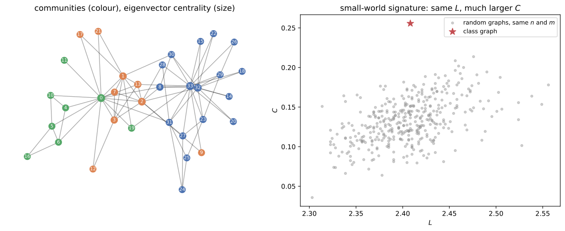
Left: the acquaintance graph, node colour giving the modularity communities and node area giving eigenvector centrality. Right: \(C\) against \(L\) for 390 connected random graphs with the same node and link counts, with the real graph starred; the real graph has the same average path length but roughly double the clustering.
The star sits directly above the random cloud: \(L\) is indistinguishable from random (\(2.408\) against \(2.406 \pm 0.042\)) while \(C\) is \(4.35\) standard deviations above it. The graph is shot through with triangles, which ought to make it parochial, and yet the eleven ties crossing the faction boundary hold the path length at the random-graph value. At \(n = 34\) this demonstrates the metrics rather than the \(\log n\) scaling of Section 9.2.1, and the community count is algorithm-dependent: Girvan–Newman stops at two groups of \(15\) and \(19\), also \(32\) of \(34\) correct but erring on nodes \(2\) and \(8\).
Problem 9.4 — Kleinberg model
Kleinberg model.
In this question, \(\log(\cdot)\) is in base \(2\) and \(\ln(\cdot)\) is in base \(e\). Consider the two-dimensional lattice in Figure 9.15 with \(n^2\) nodes labeled with their coordinates \((1,1),(1,2),\dots,(n,n)\). Figure 9.15 draws the square grid with \((1,1)\) at the top-left corner, \((1,n)\) at the top-right, \((n,1)\) at the bottom-left and \((n,n)\) at the bottom-right, every node joined to its horizontal and vertical grid neighbours. The distance between two nodes \(u=(x_1,y_1)\) and \(v=(x_2,y_2)\) is \(d(u,v)=|x_1-x_2|+|y_1-y_2|\).
(a) What is the number of nodes of distance \(1\) from node \((1,1)\), excluding itself? How about the numbers of nodes of distances \(2\) and \(3\), and of general distance \(i\), where \(1\le i\le n\)?
(b) Let \(B_j\) be the set of nodes of distance at most \(2^j\) from node \((1,1)\), excluding itself. Calculate the size of \(B_j\) for \(0\le j\le \log n\). Use the summation identity \(\sum_{k=1}^{r}k=r(r+1)/2\).
(c) Let \(R_j\) be the set of nodes contained in \(B_j\) but outside \(B_{j-1}\), i.e. \(R_j=B_j\setminus B_{j-1}\) for \(j\ge 1\), and \(R_0=B_0\). Calculate a lower bound on the size of \(R_j\). Specifically, if you obtain something of the form \(2^s+2^t\) with \(s>t>0\), you should report \(2^s\) as your answer.
(d) Let \(\alpha=2\). According to the Kleinberg model, given that two nodes \(u\) and \(v\) are separated by distance \(r\), the probability of the nodes being connected by a random link is lower bounded as follows:
\begin{equation*} \Pr(u\leftrightarrow v)\ \ge\ \frac{r^{-\alpha}}{4\ln(6n)} . \end{equation*}
Given that node \((1,1)\) has only one random link, use the result from (c) to lower bound the probability that node \((1,1)\) has a random link to a node in \(R_j\), \(\Pr(u\leftrightarrow R_j)\), for \(0\le j\le\log n\). Does the answer depend on the value of \(j\)?
(e) What happens to the result in (d) if \(\alpha=1\) or \(\alpha=3\)? (difficulty: \(\star\star\star\))
(a) \(N(i) = i+1\) for \(1 \le i \le n-1\), so \(N(1)=2\), \(N(2)=3\), \(N(3)=4\). Writing a node as \((1+a,1+b)\) with \(0\le a,b\le n-1\), its distance from the corner is \(a+b\), and the nodes at distance \(i\) are the integer points of the segment \(a+b=i\) inside the square:
\begin{equation*} N(i)=\begin{cases} i+1, & 1\le i\le n-1,\\[2pt] 2n-1-i, & n\le i\le 2n-2.\end{cases} \end{equation*}
The second branch appears because \((1,1)\) is a corner: the diagonal wavefront grows by one node per step until it runs off the far edges. The stated range’s last point is affected (\(N(n) = n-1\), not \(n+1\)), but everything below uses radii \(2^j \le n-1\), where \(N(i) = i+1\) is operative.
(b) Summing the wavefronts up to radius \(2^j\) with the given identity,
\begin{equation*} |B_j|=\sum_{i=1}^{2^j}(i+1)=\frac{2^j(2^j+1)}{2}+2^j=2^{2j-1}+2^{j-1}+2^{j}=2^{2j-1}+3\cdot 2^{j-1}. \end{equation*}
valid for \(2^j\le n-1\) (at \(j=\log n\) it slightly overcounts, which does not affect the scaling in \(j\)). Check: \(j=0\) gives \(2\), the corner’s two neighbours, and \(j=1\) gives \(5\).
(c) For \(j\ge 1\),
\begin{equation*} |R_j|=|B_j|-|B_{j-1}| =\left(2^{2j-1}+3\cdot 2^{j-1}\right)-\left(2^{2j-3}+3\cdot 2^{j-2}\right) =3\cdot 2^{2j-3}+3\cdot 2^{j-2}. \end{equation*}
Since \(3\cdot 2^{2j-3}=2^{2j-2}+2^{2j-3}\ge 2^{2j-2}\) and \(3\cdot 2^{j-2}\ge 2^{j-1}\), this is bounded below in the requested form:
\begin{equation*} |R_j|\ \ge\ 2^{2j-2}+2^{j-1},\qquad s=2j-2>t=j-1>0\ \ (j\ge 2), \end{equation*}
so the answer to report is \(|R_j|\ \ge\ 2^{2j-2}=\tfrac14\,4^{\,j}\): the annulus holds a number of nodes proportional to the square of its radius, the lattice being two-dimensional.
(d) Every node of \(R_j\) lies at distance \(r\le 2^j\) and \(r^{-2}\) decreases in \(r\), so each \(v\in R_j\) has
\begin{equation*} \Pr(u\leftrightarrow v)\ \ge\ \frac{(2^{j})^{-2}}{4\ln(6n)}=\frac{2^{-2j}}{4\ln(6n)} . \end{equation*}
With exactly one random link the events “the link goes to \(v\)” are disjoint over \(v\), so their probabilities add:
\begin{equation*} \begin{aligned} \Pr(u\leftrightarrow R_j)=\sum_{v\in R_j}\Pr(u\leftrightarrow v) &\ \ge\ |R_j|\cdot\frac{2^{-2j}}{4\ln(6n)} \\ &\ \ge\ \frac{2^{2j-2}\,2^{-2j}}{4\ln(6n)}=\frac{1}{16\ln(6n)} . \end{aligned} \end{equation*}
No, this does not depend on \(j\), which is the point of \(\alpha=2\): the node count at scale \(2^j\) grows like \(4^{j}\) while the per-node probability decays like \(4^{-j}\), and the two cancel, so the single long-range link is about equally likely to land in any of the \(\log n\) scales. That is Section 9.2.2’s cancellation made quantitative, and it is why greedy routing works – at every scale there is probability at least \(1/(16\ln 6n)\) of a link halving the remaining distance, giving delivery time \(O(\log^2 n)\).
(e) Redoing the last line with general \(\alpha\), keeping \(|R_j|\ge 2^{2j-2}\) and \(r\le 2^j\):
\begin{equation*} \Pr(u\leftrightarrow R_j)\ \ge\ \frac{2^{2j-2}\,2^{-\alpha j}}{4\ln(6n)}=\frac{2^{(2-\alpha)j-2}}{4\ln(6n)} . \end{equation*}
At \(\alpha=1\) this grows geometrically in \(j\), pushing the link to the largest scales – a nearly uniform long-range link, Watts–Strogatz style, which shortens the first hops enormously and is useless near the target. At \(\alpha=3\) the exponent is negative and the bound decays geometrically: links are almost always local, so greedy search has to crawl. Since a decaying lower bound proves nothing on its own, the matching upper bounds are Kleinberg’s theorem (delivery time \(\Omega(n^{\varepsilon(\alpha)})\) for every \(\alpha\ne d\) against \(O(\log^2 n)\) at \(\alpha=d\)); normalising the model exactly instead shows the effect directly.
import numpy as np
import matplotlib.pyplot as plt

n = 1024                                   # n x n lattice, source at the corner (1,1)
i = np.arange(1, 2*n - 1)                  # possible L1 distances from a corner
cnt = np.where(i <= n-1, i + 1, 2*n - 1 - i).astype(float)   # nodes at distance i

def ring_probs(alpha):
    w = cnt * i.astype(float)**(-alpha)
    w = w/w.sum()
    J = int(np.log2(n))
    out = []
    for j in range(J + 1):
        lo = 0 if j == 0 else 2**(j-1)      # R_j = distances in (2^(j-1), 2^j]
        sel = (i > lo) & (i <= 2**j)
        out.append(w[sel].sum())
    return np.array(out)

print('exact Kleinberg link probabilities Pr(link lands in R_j), n = %d' % n)
print('  j : ' + ''.join('%9d' % j for j in range(int(np.log2(n)) + 1)))
for a in (1, 2, 3):
    print('a=%d : ' % a + ''.join('%9.4f' % v for v in ring_probs(a)))
print('lower bound of part (d), 1/(16 ln 6n) = %.5f' % (1/(16*np.log(6*n))))
p2 = ring_probs(2)
print('alpha=2: min over j = %.4f, max = %.4f, ratio max/min = %.2f'
      % (p2.min(), p2.max(), p2.max()/p2.min()))
for a in (1, 3):
    p = ring_probs(a)
    print('alpha=%d: ratio max/min = %.1f, mass in the top ring = %.3f, in R_0 = %.4f'
          % (a, p.max()/p.min(), p[-1], p[0]))

plt.figure(figsize=(7, 4.5))
J = np.arange(int(np.log2(n)) + 1)
for a, mk in zip((1, 2, 3), ('o', 's', '^')):
    plt.semilogy(J, ring_probs(a), marker=mk, label=r'$\alpha=%d$' % a)
plt.axhline(1/(16*np.log(6*n)), ls='--', color='gray', label=r'bound $1/(16\ln 6n)$')
plt.xlabel(r'scale $j$  (ring $R_j$: distance in $(2^{j-1},2^j]$)')
plt.ylabel(r'$\Pr(\mathrm{random\ link}\in R_j)$')
plt.title(r'Kleinberg model on a $%d\times%d$ lattice, source at a corner' % (n, n))
plt.legend(); plt.grid(alpha=0.3)
plt.savefig('nl-ch09-kleinberg-scale-balance.svg', dpi=150, bbox_inches='tight')
exact Kleinberg link probabilities Pr(link lands in R_j), n = 1024
  j :         0        1        2        3        4        5        6        7        8        9       10
a=1 :    0.0014   0.0011   0.0018   0.0033   0.0061   0.0117   0.0229   0.0454   0.0903   0.1800   0.3596
a=2 :    0.2114   0.0793   0.0800   0.0781   0.0761   0.0748   0.0741   0.0737   0.0735   0.0734   0.0733
a=3 :    0.7027   0.1318   0.0795   0.0426   0.0218   0.0110   0.0055   0.0027   0.0014   0.0007   0.0003
lower bound of part (d), 1/(16 ln 6n) = 0.00716
alpha=2: min over j = 0.0733, max = 0.2114, ratio max/min = 2.88
alpha=1: ratio max/min = 341.8, mass in the top ring = 0.360, in R_0 = 0.0014
alpha=3: ratio max/min = 2048.0, mass in the top ring = 0.000, in R_0 = 0.7027
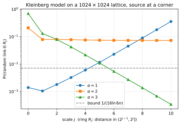
Exact probability that the single long-range link from the corner lands in the annulus \(R_j\), against the scale \(j\), on a \(1024\times 1024\) lattice. At \(\alpha=2\) the curve is flat across ten octaves of distance; at \(\alpha=1\) it grows like \(2^{j}\) and at \(\alpha=3\) it decays like \(2^{-j}\), exactly the factor \(2^{(2-\alpha)j}\) of part (e). The dashed line is the crude bound \(1/(16\ln 6n)\) from part (d).
The \(\alpha=2\) row is flat to within a factor of \(1.09\) across \(j=1,\dots,10\) (the \(j=0\) entry is larger only because \(R_0\) holds the two neighbours at distance \(1\), where \(r^{-2}\) is maximal), and every entry clears part (d)’s bound \(0.00716\) by an order of magnitude, as a bound built from two worst cases should. At \(\alpha=1\) the largest ring absorbs \(36\%\) of the mass against \(0.1\%\) innermost; at \(\alpha=3\) it is reversed, \(70\%\) within distance \(1\). Only the middle case gives every scale a share bounded away from zero, and that scale-invariance is what makes the network searchable.
Problem 9.5 — De Bruijn sequence, Eulerian cycle, and card magic
De Bruijn sequence, Eulerian cycle, and card magic.
A de Bruijn sequence of order \(k\) is a binary vector of \(2^k\) 0s or 1s, such that each sequence of \(k\) 0s or 1s appears only once in the vector (wrapping around the corner). For example, \(0011\) is a de Bruijn sequence of order \(k=2\) because each of the sequences \(00,01,10,11\) appears only once, as shown in Figure 9.16, which draws the four bits around a circle with a length-2 window sliding clockwise.
There are two basic questions regarding de Bruijn sequences: for any order \(k\), (1) do they exist? and (2) how can we find one?
The answers can be obtained by studying a de Bruijn graph. Consider the case of \(k=3\) with the corresponding two-dimensional de Bruijn graph shown in Figure 9.17. That graph is directed, with four nodes labelled \(00\) (top), \(10\) (left), \(01\) (right) and \(11\) (bottom), and eight labelled edges: a self-loop at \(00\) labelled \(0\); \(00\to 01\) labelled \(1\); \(01\to 10\) labelled \(0\); \(01\to 11\) labelled \(1\); \(10\to 00\) labelled \(0\); \(10\to 01\) labelled \(1\); \(11\to 10\) labelled \(0\); and a self-loop at \(11\) labelled \(1\). In general the node is the last two bits written and an edge labelled \(b\) goes from node \(xy\) to node \(yb\).
We traverse the graph (starting at any node) while writing down the labels (0 or 1) on the edges. It is not difficult to see that for any Eulerian cycle on the graph, i.e. a traversal of the nodes through a cycle using every edge once and only once, the corresponding sequence of edge labels is a de Bruijn sequence. Hence the problem of finding a de Bruijn sequence reduces to finding an Eulerian cycle in the corresponding de Bruijn graph, and this answers question (2). For question (1), the answer is affirmative if every de Bruijn graph has an Eulerian cycle, which indeed is true because each node’s in-degree and out-degree are equal (a basic result in graph theory due to Euler).
So what are de Bruijn sequences good for? Among their important applications is a famous card trick, where the magician can name the card held by \(k\) people in the audience even after random cuts have been made to the deck of cards. (The details can be found in a unique book by Persi Diaconis and Ron Graham, Magical Mathematics: The Mathematical Ideas that Animate Great Magic Tricks, Princeton University Press, 2011.)
Now, your task for this homework problem is simple: for \(k=3\) there are two distinct de Bruijn sequences. What do we mean by “distinct sequences”? Sequences \(01011\) and \(00111\) are distinct, but sequences \(01011\) and \(10101\) are not (try to write out the sequences as in Figure 9.16). Draw two distinct Eulerian cycles on the graph in Figure 9.17, and report the two distinct de Bruijn sequences found. (difficulty: \(\star\star\))
The two sequences are
\begin{equation*} 00010111 \qquad\text{and}\qquad 00011101 , \end{equation*}
and each is the reversal of the other: \(00010111\) read backwards is \(11101000\), a rotation of \(00011101\). Both cycles below start at node \(00\) and use all eight edges once.
Cycle A, giving \(01011100\) (a rotation of \(00010111\)):
\begin{equation*} 00\xrightarrow{0}00\xrightarrow{1}01\xrightarrow{0}10\xrightarrow{1}01\xrightarrow{1}11\xrightarrow{1}11\xrightarrow{0}10\xrightarrow{0}00 . \end{equation*}
Cycle B, giving \(01110100\) (a rotation of \(00011101\)):
\begin{equation*} 00\xrightarrow{0}00\xrightarrow{1}01\xrightarrow{1}11\xrightarrow{1}11\xrightarrow{0}10\xrightarrow{1}01\xrightarrow{0}10\xrightarrow{0}00 . \end{equation*}
The only choice in either traversal is at the first visit to node \(01\), going to \(10\) (cycle A) or to \(11\) (cycle B); everything after is forced, since once one of a node’s two out-edges is spent the other is the only exit. That single binary choice is why there are exactly two sequences, matching the general count \(2^{2^{k-1}-k}=2\) at \(k=3\). Traversing \(xy\xrightarrow{b}yb\) writes the \(3\)-window \(xyb\), so using every edge once writes each of the eight triples once, with the return to the start making the reading wrap correctly.
Enumerating, to confirm these are the only two:
from itertools import product

nodes = [''.join(p) for p in product('01', repeat=2)]
edges = [(u, b, u[1] + b) for u in nodes for b in '01']       # (from, label, to)
print('edges:', ', '.join('%s -%s-> %s' % e for e in edges))

def euler_circuits(start):
    out = []
    def walk(v, used, path):
        if len(used) == len(edges):
            if v == start:
                out.append(list(path))
            return
        for k, (a, b, w) in enumerate(edges):
            if a == v and k not in used:
                walk(w, used | {k}, path + [k])
    walk(start, frozenset(), [])
    return out

seq_of = lambda circ: ''.join(edges[k][1] for k in circ)
canon  = lambda s: min(s[i:] + s[:i] for i in range(len(s)))

circuits = euler_circuits('00')
classes = {}
for c in circuits:
    classes.setdefault(canon(seq_of(c)), []).append(c)
print('Eulerian circuits from node 00: %d, falling into %d rotation classes'
      % (len(circuits), len(classes)))
for s in sorted(classes):
    rep = classes[s][0]
    trail = ' -> '.join(edges[k][0] for k in rep) + ' -> 00'
    print('  sequence %s   read off the cycle as %s' % (s, seq_of(rep)))
    print('    cycle: ' + trail)
    win = [(s + s)[i:i+3] for i in range(8)]
    print('    windows: %s  (all distinct: %s)' % (' '.join(win), len(set(win)) == 8))

a, b = sorted(classes)
print('is %s a rotation of %s ? %s' % (b, a, b in [a[i:] + a[:i] for i in range(8)]))
edges: 00 -0-> 00, 00 -1-> 01, 01 -0-> 10, 01 -1-> 11, 10 -0-> 00, 10 -1-> 01, 11 -0-> 10, 11 -1-> 11
Eulerian circuits from node 00: 4, falling into 2 rotation classes
  sequence 00010111   read off the cycle as 01011100
    cycle: 00 -> 00 -> 01 -> 10 -> 01 -> 11 -> 11 -> 10 -> 00
    windows: 000 001 010 101 011 111 110 100  (all distinct: True)
  sequence 00011101   read off the cycle as 01110100
    cycle: 00 -> 00 -> 01 -> 11 -> 11 -> 10 -> 01 -> 10 -> 00
    windows: 000 001 011 111 110 101 010 100  (all distinct: True)
is 00011101 a rotation of 00010111 ? False
Four Eulerian circuits leave node \(00\) but collapse to two sequences, since the cycle passes through \(00\) twice and either visit may start the same necklace. The window lists show all eight triples appearing once each, and the last line confirms the two are distinct in the problem’s sense rather than rotations.
import numpy as np
import matplotlib.pyplot as plt
from matplotlib.patches import FancyArrowPatch, Circle

pos = {'00': (0, 1), '10': (-1, 0), '01': (1, 0), '11': (0, -1)}
rad = {('01','10'): 0.25, ('10','01'): 0.25}
cycles = {'00010111': ['00','00','01','10','01','11','11','10','00'],
          '00011101': ['00','00','01','11','11','10','01','10','00']}

fig, axes = plt.subplots(1, 2, figsize=(11, 5.2))
for ax, (seq, trail) in zip(axes, cycles.items()):
    for name, (x, y) in pos.items():
        ax.add_patch(Circle((x, y), 0.16, fc='white', ec='black', zorder=3))
        ax.text(x, y, name, ha='center', va='center', zorder=4, fontsize=11)
    for step in range(8):
        u, v = trail[step], trail[step+1]
        lab = v[1]
        if u == v:                                   # self loop
            x, y = pos[u]
            s = 1 if y > 0 else -1
            ax.add_patch(FancyArrowPatch((x-0.12, y+0.11*s), (x+0.12, y+0.11*s),
                         connectionstyle='arc3,rad=%.1f' % (-2.6*s),
                         arrowstyle='-|>', mutation_scale=13, color='#C44E52', lw=1.6))
            ax.text(x, y + 0.62*s, '%d: label %s' % (step+1, lab),
                    ha='center', va='center', fontsize=9, color='#C44E52')
        else:
            r = rad.get((u, v), 0.0)
            ax.add_patch(FancyArrowPatch(pos[u], pos[v], shrinkA=13, shrinkB=13,
                         connectionstyle='arc3,rad=%.2f' % r,
                         arrowstyle='-|>', mutation_scale=13, color='#4C72B0', lw=1.6))
            mx, my = (pos[u][0]+pos[v][0])/2, (pos[u][1]+pos[v][1])/2
            # (nx_, ny_) is the direction a curved arc bulges toward, so a curved
            # label sits on its own arc and a straight label sits outside the diamond
            nx_, ny_ = pos[v][1]-pos[u][1], pos[u][0]-pos[v][0]
            nn = np.hypot(nx_, ny_)
            off = -0.20 if r == 0 else 0.34
            ax.text(mx + off*nx_/nn, my + off*ny_/nn, '%d: %s' % (step+1, lab),
                    ha='center', va='center', fontsize=9, color='#4C72B0')
    ax.set_title('cycle giving %s' % seq)
    ax.set_xlim(-1.8, 1.8); ax.set_ylim(-1.9, 1.9); ax.set_aspect('equal'); ax.axis('off')
plt.tight_layout()
plt.savefig('nl-ch09-debruijn-eulerian-cycles.svg', dpi=150, bbox_inches='tight')
print('order of edge labels, cycle A:', ''.join(t[1] for t in cycles['00010111'][1:]))
print('order of edge labels, cycle B:', ''.join(t[1] for t in cycles['00011101'][1:]))
order of edge labels, cycle A: 01011100
order of edge labels, cycle B: 01110100
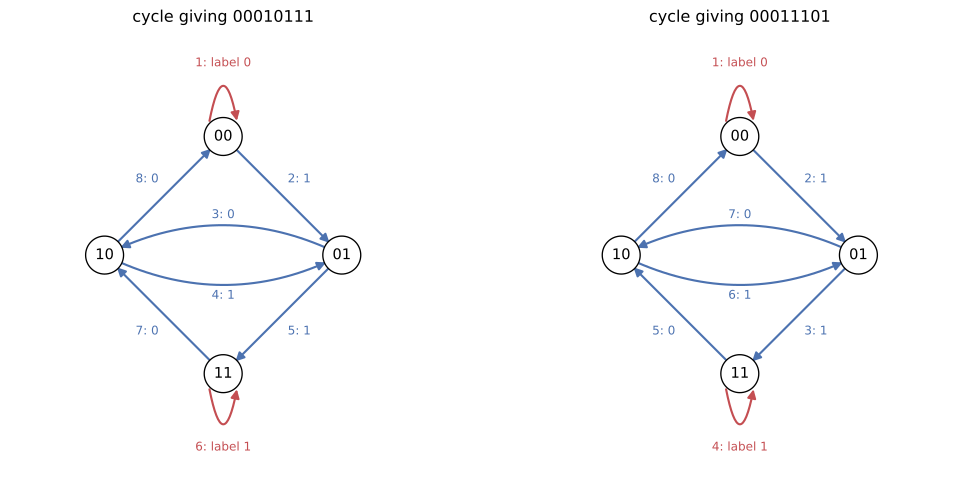
The two Eulerian cycles on the order-3 de Bruijn graph of Figure 9.17, with each edge annotated by its position in the traversal and its label. The cycles differ only in which edge is taken out of node \(01\) on the first visit; reading the labels in order gives \(01011100\) and \(01110100\), i.e. the sequences \(00010111\) and \(00011101\).
Does the Internet have an Achilles heel?
Problem 10.1 — Probability distributions
Probability distributions. The log-normal distribution has a probability density function given by \[ f(x) = \frac{1}{x\sqrt{2\pi}\,\sigma}\, e^{-\frac{(\ln x-\mu)^2}{2\sigma^2}} \] and cumulative density function given by \(\Phi\!\left(\frac{\ln x-\mu}{\sigma}\right)\), where \(\Phi\) is the cumulative density function of the normal distribution. Parameters \(\mu\) and \(\sigma\) are the mean and standard deviation of the corresponding normal distribution.
Plot the probability density functions of the following distributions on domain \([1,5]\) with granularity \(0.01\) (all on the same graph for contrast), first using a linear and then using a (natural) log–log scale:
- Pareto distribution with \(x_m=1\), \(\alpha=1\);
- normal distribution with \(\mu=1\), \(\sigma=1\); and
- log-normal distribution with \(\mu=1\), \(\sigma=1\).
Does the tail of the log-normal distribution look like the normal distribution or the Pareto distribution? (difficulty: \(\star\))
The tail of the log-normal looks like the Pareto, not like the normal.
The three densities on \([1,5]\) are
\begin{equation*} \begin{aligned} f_{\text{Par}}(x)&=\alpha x_m^{\alpha}x^{-(\alpha+1)}=x^{-2}, \\ f_{\text{N}}(x)&=\frac{1}{\sqrt{2\pi}}e^{-(x-1)^2/2}, \\ f_{\text{LN}}(x)&=\frac{1}{x\sqrt{2\pi}}e^{-(\ln x-1)^2/2}, \end{aligned} \end{equation*}
the first being equation (10.2) with \(k=x_m=1\). The diagnostic is the local log–log slope \(s(x)=d\log f/d\log x\), a straight log–log line being the visual signature of a power law (Figure 10.2):
\[ s_{\text{Par}}(x) = -(\alpha+1) = -2, \] \[ s_{\text{N}}(x) = -x(x-\mu) = -x(x-1), \] \[ s_{\text{LN}}(x) = -1-\frac{\ln x-\mu}{\sigma^2} = -1-(\ln x - 1) . \]
The Pareto slope is flat, the normal steepens like \(x^2\), and the log-normal steepens only like \(\ln x\), which over a bounded window is nearly constant: on log–log axes the log-normal is a parabola in \(\log x\) of curvature \(-1/\sigma^2\), and a gently curved parabola is indistinguishable from a line over a decade or two.
import numpy as np
import matplotlib.pyplot as plt

x = np.arange(1.0, 5.0 + 1e-9, 0.01)
mu, sig, alpha, xm = 1.0, 1.0, 1.0, 1.0

pareto = alpha * xm**alpha * x**(-(alpha + 1.0))
normal = np.exp(-(x - mu)**2 / (2*sig**2)) / (np.sqrt(2*np.pi)*sig)
lognrm = np.exp(-(np.log(x) - mu)**2 / (2*sig**2)) / (x*np.sqrt(2*np.pi)*sig)

fig, ax = plt.subplots(1, 2, figsize=(11, 4.2))
for a, sc in zip(ax, ['linear', 'log']):
    a.plot(x, pareto, label='Pareto $x_m=1,\\ \\alpha=1$')
    a.plot(x, normal, label='normal $\\mu=1,\\ \\sigma=1$')
    a.plot(x, lognrm, label='log-normal $\\mu=1,\\ \\sigma=1$')
    a.set_xlabel('$x$'); a.set_ylabel('pdf $f(x)$')
    if sc == 'log':
        a.set_xscale('log'); a.set_yscale('log'); a.set_title('log-log scale')
    else:
        a.set_title('linear scale')
    a.legend(fontsize=8); a.grid(alpha=.3)
plt.tight_layout()
plt.savefig('nl-ch10-longtail-pdfs.svg', dpi=150, bbox_inches='tight')

def slope(y):
    return np.gradient(np.log(y), np.log(x))

print('  x     Pareto    normal   lognorm     |  local log-log slopes')
for xv in [1.0, 2.0, 3.0, 4.0, 5.0]:
    k = int(round((xv-1.0)/0.01))
    print(f'{x[k]:4.1f}  {pareto[k]:8.4f} {normal[k]:9.5f} {lognrm[k]:9.5f}   |'
          f' {slope(pareto)[k]:7.2f} {slope(normal)[k]:8.2f} {slope(lognrm)[k]:8.2f}')
print()
print('ratio f(5)/f(1):  Pareto %.4f   normal %.6f   log-normal %.4f'
      % (pareto[-1]/pareto[0], normal[-1]/normal[0], lognrm[-1]/lognrm[0]))

# how well does a straight line on log-log axes describe each density?
print()
print('best straight-line fit on log-log axes over [1,5]:')
for nm, y in [('log-normal', lognrm), ('Pareto', pareto), ('normal', normal)]:
    p = np.polyfit(np.log(x), np.log(y), 1)
    resid = np.max(np.abs(np.log(y) - np.polyval(p, np.log(x))))
    print('  %-10s fitted slope %+.2f   max residual in ln f  %.3f' % (nm, p[0], resid))
cross = x[np.where(np.diff(np.sign(lognrm - pareto)))[0] + 1]
print()
print('log-normal overtakes Pareto at x = %.2f' % cross[0])
for xv in [3.0, 4.0]:
    k = int(round((xv-1.0)/0.01))
    print('at x=%.0f: Pareto/normal = %5.1f   log-normal/normal = %5.1f'
          % (xv, pareto[k]/normal[k], lognrm[k]/normal[k]))
  x     Pareto    normal   lognorm     |  local log-log slopes
 1.0    1.0000   0.39894   0.24197   |   -2.00    -0.01    -0.00
 2.0    0.2500   0.24197   0.19030   |   -2.00    -2.00    -0.69
 3.0    0.1111   0.05399   0.13234   |   -2.00    -6.00    -1.10
 4.0    0.0625   0.00443   0.09256   |   -2.00   -12.00    -1.39
 5.0    0.0400   0.00013   0.06627   |   -2.00   -19.96    -1.61

ratio f(5)/f(1):  Pareto 0.0400   normal 0.000335   log-normal 0.2739

best straight-line fit on log-log axes over [1,5]:
  log-normal fitted slope -0.89   max residual in ln f  0.293
  Pareto     fitted slope -2.00   max residual in ln f  0.000
  normal     fitted slope -4.92   max residual in ln f  2.387

log-normal overtakes Pareto at x = 2.52
at x=3: Pareto/normal =   2.1   log-normal/normal =   2.5
at x=4: Pareto/normal =  14.1   log-normal/normal =  20.9
![Pareto (\(x_m=1,\alpha=1\)), normal (\(\mu=\sigma=1\)) and log-normal (\(\mu=\sigma=1\)) densities on \([1,5]\), plotted on linear axes (left) and log–log axes (right). On log–log axes the Pareto is exactly straight, the log-normal is a very gently bending curve that stays close to it, and the normal collapses off the bottom of the plot.](/words/library/books/nl-ch10-longtail-pdfs.svg)
Pareto (\(x_m=1,\alpha=1\)), normal (\(\mu=\sigma=1\)) and log-normal (\(\mu=\sigma=1\)) densities on \([1,5]\), plotted on linear axes (left) and log–log axes (right). On log–log axes the Pareto is exactly straight, the log-normal is a very gently bending curve that stays close to it, and the normal collapses off the bottom of the plot.
Three readings confirm it. Across \([1,5]\) the normal density falls by a factor of about \(3000\) against \(25\) for the Pareto and \(3.65\) for the log-normal. The log-normal’s local slope moves only from \(0\) to \(-1.61\) across the whole window, a barely perceptible bend, while the normal’s moves from \(0\) to \(-20\); least squares on log–log axes gives the log-normal slope \(-0.89\) with worst residual \(0.29\) in \(\ln f\) against the normal’s \(-4.92\) with \(2.39\), so a naive experimenter would report a power law of exponent about \(-0.9\). And beyond \(x=2.52\) the log-normal sits above the Pareto for the rest of the window, while the normal falls a factor of \(14\) below the Pareto and \(21\) below the log-normal by \(x=4\).
The log-normal is nonetheless not a power law: its slope \(-1-(\ln x-\mu)/\sigma^2\) diverges to \(-\infty\), only arbitrarily slowly, so no fixed \(\alpha\) satisfies \(\mathrm{Prob}[X\ge x]\approx kx^{-\alpha}\) in the limit of equation (10.1). Over a bounded measurement range it masquerades as one, the more convincingly the larger \(\sigma\) is – the Mandelbrot–Simon point of Section 10.2.4: a straight line on a log–log plot does not identify the generative mechanism.
Problem 10.2 — Utility maximization under linear constraints
Utility maximization under linear constraints. We will examine another generative model for power-law distributions. Consider the case of nodes communicating to each other over a set of shared links. Each node’s utility is a function of the rate it receives. Specifically, we choose the \(\alpha\)-fair (also called isoelastic) utility function, where \(\alpha \ge 0\) is a fairness parameter. We will talk much more about these functions in Chapter 11. We can formulate this as \[ \begin{array}{ll}\text{maximize}_{\mathbf{x}} & \displaystyle\sum_j \frac{x_j^{1-\alpha}}{1-\alpha}\\[4pt] \text{subject to} & \mathbf{A}\mathbf{x}\le \mathbf{b}\\ & \mathbf{x}\ge \mathbf{0},\end{array} \] where \(b_i\) is the capacity of link \(i\), \(x_j\) is the rate of session \(j\), and \(\mathbf{A}\) is a binary routing matrix between sessions and links: \[ A_{ij}=\begin{cases}1 & \text{if session } j \text{ is present on link } i\\ 0 & \text{otherwise.}\end{cases} \] Show that \(x_j\) follows a power law (for fixed \(\alpha\)), and give an intuition for your answer. (difficulty: \(\star\star\))
The optimal rate is an exact power of the session’s path price, \(x_j^\star = q_j^{-1/\alpha}\), which carries a power-law tail over to the rates. This is the Lagrangian route of Section 10.4.2 with isoelastic utility in place of entropy.
Attach a multiplier \(\lambda_i\ge 0\) to each link constraint \(\sum_j A_{ij}x_j\le b_i\) and form \[ L(\mathbf{x},\boldsymbol{\lambda})=\sum_j \frac{x_j^{1-\alpha}}{1-\alpha}-\sum_i \lambda_i\Big(\sum_j A_{ij}x_j-b_i\Big). \] The objective is strictly concave and separable and the constraints are linear, so the problem is a convex program with a unique optimizer and zero duality gap; the optimizer maximizes \(L\) at the optimal \(\boldsymbol{\lambda}^\star\). Differentiating in \(x_j\): \[ \frac{\partial L}{\partial x_j}=x_j^{-\alpha}-\sum_i \lambda_i A_{ij}=0. \] Define the path price of session \(j\) as the sum of the multipliers of the links it crosses, \[ q_j \;=\; \sum_i A_{ij}\lambda_i^\star \;=\;\sum_{i\in r_j}\lambda_i^\star , \] where \(r_j\) is session \(j\)’s route. Then the optimal rate is \[ \boxed{\;x_j^\star = q_j^{-1/\alpha}\;}\tag{\(\ast\)} \]
Here \(q_j>0\) for every \(j\), since \(x^{1-\alpha}/(1-\alpha)\) is strictly increasing, so every session crosses a saturated link, whose multiplier is positive by complementary slackness.
Let \(F_q\) be the distribution of path prices across sessions. Since \(x=q^{-1/\alpha}\) decreases, a large rate means a small price: \[ \mathrm{Prob}[X\ge x]=\mathrm{Prob}\big[q^{-1/\alpha}\ge x\big]=\mathrm{Prob}\big[q\le x^{-\alpha}\big]=F_q\!\left(x^{-\alpha}\right). \] Suppose \(F_q(t)\approx c\,t^{\beta}\) as \(t\to 0^{+}\), i.e. \(F_q\) is regularly varying at the origin – the mild statement that the fraction of sessions with a nearly free route scales as a power of how free it is. Then \[ \mathrm{Prob}[X\ge x]\;\approx\; c\,x^{-\alpha\beta}, \] exactly equation (10.1)’s power-law tail with exponent \(\alpha\beta\), hence by differentiation a pdf of exponent \(-(\alpha\beta+1)\) as in (10.2). Generically \(\beta=1\): a price density finite and non-zero at \(q=0\) gives \(F_q(t)\sim ct\) and a rate tail of exponent exactly \(\alpha\), so proportional fairness (\(\alpha=1\)) yields \(\mathrm{Prob}[X\ge x]\propto x^{-1}\), Zipf’s law.
The intuition is that the isoelastic family is the only one whose marginal utility \(U’(x)=x^{-\alpha}\) is scale-free: doubling a rate multiplies marginal utility by \(2^{-\alpha}\) whatever the rate was. The optimizer equates marginal utility to path price, so price \(\mapsto\) rate inverts a scale-free function and is therefore itself a power – twice the congestion price buys \(2^{-1/\alpha}\) times the rate for a backbone flow and an edge flow alike, leaving no characteristic rate anywhere. Under exponential utility \(U(x)=-e^{-x}\) instead, \(x^\star=-\ln q\) and the allocation acquires a characteristic scale. Note also that \(q_j\) is a sum over the hops of \(r_j\), so a spread in route lengths is exponentiated into a spread in rates; and that no growth process or rich-get-richer appears anywhere, this being a constrained-optimization model in the sense of Figure 10.6.
Solving the \(\alpha\)-fair problem on a random 70-node geometric graph with shortest-path routing and 500 sessions, through the dual \(D(\boldsymbol{\lambda})=\frac{\alpha}{1-\alpha}\sum_j q_j^{1-1/\alpha}+\boldsymbol{\lambda}^{T}\mathbf{b}\) with gradient \(b_i-\sum_j A_{ij}x_j\), checks both \((\ast)\) and the prediction \(\mathrm{Prob}[X\ge x]=F_q(x^{-\alpha})\).
import numpy as np, networkx as nx
from scipy.optimize import minimize
import matplotlib.pyplot as plt
rng = np.random.default_rng(7)

G = nx.random_geometric_graph(70, 0.28, seed=3)
G = G.subgraph(max(nx.connected_components(G), key=len)).copy()
links = list(G.edges()); Lk = {e: i for i, e in enumerate(links)}
def lid(u, v): return Lk[(u, v)] if (u, v) in Lk else Lk[(v, u)]
nodes = list(G.nodes()); M = 500; routes = []
while len(routes) < M:
    s, d = rng.choice(nodes, 2, replace=False)
    p = nx.shortest_path(G, int(s), int(d))
    if len(p) > 1:
        routes.append([lid(p[k], p[k+1]) for k in range(len(p)-1)])
A = np.zeros((len(links), M))
for j, r in enumerate(routes): A[r, j] = 1.0
b = rng.uniform(0.5, 2.0, len(links))

def dual_solve(alpha):
    def F(lam):
        q = A.T @ lam
        x = q**(-1.0/alpha)
        if abs(alpha - 1.0) < 1e-12:
            val = -np.sum(np.log(q)) - M + lam @ b
        else:
            val = (alpha/(1-alpha))*np.sum(q**(1-1/alpha)) + lam @ b
        return val, b - A @ x
    r = minimize(F, np.full(len(links), 1.0), jac=True, method='L-BFGS-B',
                 bounds=[(1e-9, None)]*len(links),
                 options=dict(maxiter=20000, ftol=1e-16, gtol=1e-12))
    lam = r.x; q = A.T @ lam
    return q**(-1.0/alpha), q, A @ (q**(-1.0/alpha))

print('network solve: %d links, %d sessions' % (len(links), M))
fig, ax = plt.subplots(1, 2, figsize=(11, 4.2))
for alpha, c in zip([1.0, 2.0, 3.0], ['C0', 'C1', 'C2']):
    x, q, y = dual_solve(alpha)
    lo, hi = int(0.02*M), int(0.4*M)
    xs = np.sort(x)[::-1]; cc = np.arange(1, M+1)/M
    sl = np.polyfit(np.log(xs[lo:hi]), np.log(cc[lo:hi]), 1)[0]
    beta = np.polyfit(np.log(np.sort(q)[lo:hi]), np.log(np.arange(lo, hi)/M), 1)[0]
    print(f'  alpha={alpha:.0f}: max capacity violation {np.max(y-b):+.1e},'
          f'  max |x_j - q_j^(-1/alpha)| = {np.max(np.abs(x-q**(-1/alpha))):.1e}')
    print(f'          measured rate-tail slope {sl:+.3f} | price exponent beta {beta:+.3f}'
          f' | predicted -alpha*beta {-alpha*beta:+.3f}')
    ax[0].loglog(q, x, '.', ms=3, color=c, label=f'$\\alpha={alpha:.0f}$')
    qq = np.logspace(np.log10(q.min()), np.log10(q.max()), 40)
    ax[0].loglog(qq, qq**(-1/alpha), '--', color='k', lw=.8)
    ax[1].loglog(xs, cc, '.', ms=3, color=c, label=f'$\\alpha={alpha:.0f}$')
ax[0].set_xlabel('path price $q_j=\\sum_{i\\in r_j}\\lambda_i^\\star$')
ax[0].set_ylabel('optimal rate $x_j^\\star$')
ax[0].set_title('rates lie exactly on $x=q^{-1/\\alpha}$')
ax[0].legend(fontsize=8); ax[0].grid(alpha=.3, which='both')
ax[1].set_xlabel('rate $x$'); ax[1].set_ylabel('$\\mathrm{Prob}[X\\geq x]$')
ax[1].set_title('tail distribution of session rates')
ax[1].legend(fontsize=8); ax[1].grid(alpha=.3, which='both')
plt.tight_layout()
plt.savefig('nl-ch10-alpha-fair-powerlaw.svg', dpi=150, bbox_inches='tight')

print()
for alpha in [0.5, 1.0, 2.0, 3.0]:
    qs = rng.uniform(0, 1, 400000)
    xx = np.sort(qs**(-1.0/alpha))[::-1]
    cc = np.arange(1, len(xx)+1)/len(xx)
    s = np.polyfit(np.log(xx[:200000]), np.log(cc[:200000]), 1)[0]
    print(f'  q ~ U(0,1), alpha={alpha}: fitted tail exponent {s:+.4f}  (theory {-alpha:+.1f})')
network solve: 438 links, 500 sessions
  alpha=1: max capacity violation +1.9e-07,  max |x_j - q_j^(-1/alpha)| = 0.0e+00
          measured rate-tail slope -0.915 | price exponent beta +0.932 | predicted -alpha*beta -0.932
  alpha=2: max capacity violation +1.7e-06,  max |x_j - q_j^(-1/alpha)| = 0.0e+00
          measured rate-tail slope -0.904 | price exponent beta +0.461 | predicted -alpha*beta -0.922
  alpha=3: max capacity violation +4.0e-04,  max |x_j - q_j^(-1/alpha)| = 0.0e+00
          measured rate-tail slope -0.899 | price exponent beta +0.306 | predicted -alpha*beta -0.917

  q ~ U(0,1), alpha=0.5: fitted tail exponent -0.5015  (theory -0.5)
  q ~ U(0,1), alpha=1.0: fitted tail exponent -1.0055  (theory -1.0)
  q ~ U(0,1), alpha=2.0: fitted tail exponent -1.9912  (theory -2.0)
  q ~ U(0,1), alpha=3.0: fitted tail exponent -2.9944  (theory -3.0)
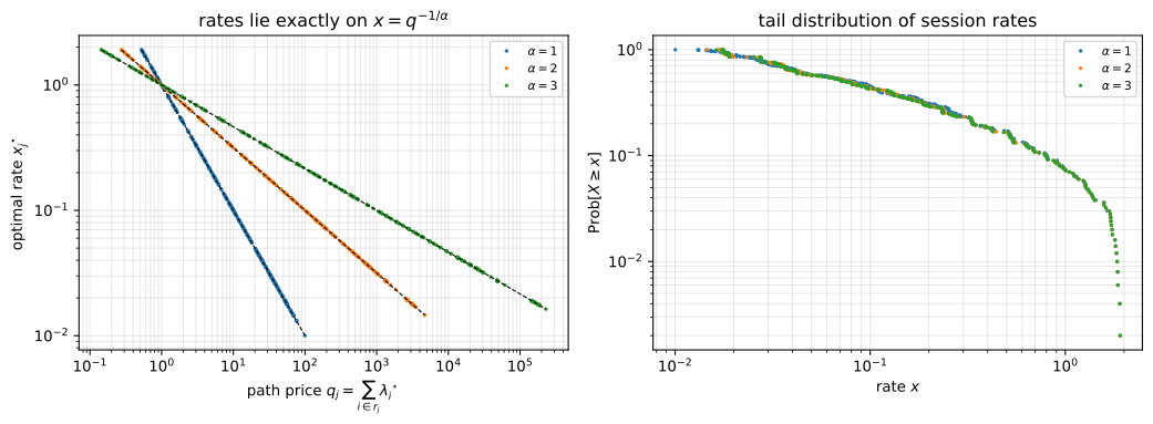
Left: optimal session rate against path price for \(\alpha=1,2,3\), on log–log axes; every point falls on the dashed line \(x=q^{-1/\alpha}\), whose slope is \(-1/\alpha\). Right: the tail distribution of the 500 session rates, straight over roughly a decade and a half — a power-law allocation produced with no growth process and no preferential attachment.
Result \((\ast)\) holds to machine precision at every \(\alpha\), and with \(q\sim U(0,1)\) the fitted tail exponents \(0.50, 1.01, 1.99, 2.99\) match the predicted \(\alpha\) to three digits. On the network the rates are power-law over more than a decade and \(\alpha\beta\) tracks the measured slope (\(-0.93\) against \(-0.92\), \(-0.92\) against \(-0.90\), \(-0.92\) against \(-0.90\)) – but the exponent is not \(\alpha\), staying near \(0.9\) throughout, because the equilibrium price distribution adjusts to \(\alpha\), \(\beta\) falling \(0.93 \to 0.46 \to 0.31\) almost as \(1/\alpha\) and leaving \(\alpha\beta\) invariant. So what is proved is \((\ast)\) plus the conditional “\(F_q\) regularly varying at \(0\) with index \(\beta\) implies rate-tail exponent \(\alpha\beta\)”; the existence of the power law is robust, its exponent is not simply \(\alpha\).
Problem 10.3 — Preferential attachment
Preferential attachment. Recall the preferential attachment model, where, with probability \(\theta\), a new node attaches to another node proportional to its in-degree. Specifically, the probability of the new node attaching to node \(k\) is \(\dfrac{d_k}{\sum_j d_j}\), where \(d_k\) is the in-degree of node \(k\). And with probability \(1-\theta\), a new node attaches to one of the existing nodes at random.
Run a simulation of preferential attachment with \(\theta=0.5\) for 500 time steps. Plot \(p_i\) versus \(i\). Does it follow the power-law distribution as expected? (difficulty: \(\star\star\))
Yes, but only in the sense that the simulated \(p_i\) reproduces the exact solution \(p_i=4/((i+1)(i+2)(i+3))\) of the balance equation; the measured log–log slope over the degrees a \(500\)-step run reaches is about \(-1.9\), not the asymptotic \(-3\).
Section 10.4.1’s balance equation (10.8) is \[ p_i\,(1+\bar\theta+i\theta)=p_{i-1}\,(\bar\theta+(i-1)\theta),\qquad \bar\theta=1-\theta. \] At \(\theta=\bar\theta=\tfrac12\) this collapses to \[ p_i\Big(\tfrac32+\tfrac i2\Big)=p_{i-1}\,\tfrac i2 \qquad\Longrightarrow\qquad \frac{p_i}{p_{i-1}}=\frac{i}{i+3}. \] Telescoping from \(p_0\), \[ p_i=p_0\prod_{k=1}^{i}\frac{k}{k+3}=p_0\,\frac{i!\;3!}{(i+3)!}=\frac{6\,p_0}{(i+1)(i+2)(i+3)} . \] Normalizing with \(\sum_{n\ge 1}\frac{1}{n(n+1)(n+2)}=\tfrac14\) gives \(\sum_i p_i = 6p_0\cdot\tfrac14=1\), so \(p_0=\tfrac23\) and
\[ \boxed{\;p_i=\frac{4}{(i+1)(i+2)(i+3)}\;}\qquad\text{for }\theta=0.5. \]
Here \(\sum_i i\,p_i = 4(\tfrac12-\tfrac14)=1\), the mean in-degree required by one node and one link per step (Check!), and \(p_i\sim 4i^{-3}\) matches equation (10.10)’s \(i^{-(1+\theta)/\theta}\) while \(q_j=\sum_{i\ge j}p_i\sim 2j^{-2}\) matches equation (10.11)’s \(j^{-1/\theta}\).
Starting from a single node with a link back to itself, each of \(500\) steps adds a node that links to an existing one, with probability \(\theta\) proportionally to in-degree and otherwise uniformly. Below are the single required run and an ensemble average over \(4000\) runs, since a \(501\)-node graph holds only a handful of nodes at any large degree.
import numpy as np
import matplotlib.pyplot as plt

def run(theta, T, rng):
    d = np.array([1.0])                       # node 0 starts with a link back to itself
    tot = 1.0
    for _ in range(T):
        if rng.random() < theta:
            k = rng.choice(len(d), p=d/tot)   # proportional to in-degree
        else:
            k = rng.integers(len(d))          # uniformly at random
        d[k] += 1.0; tot += 1.0
        d = np.append(d, 0.0)                 # the new node arrives with in-degree 0
    return d

theta, T, R = 0.5, 500, 4000
rng = np.random.default_rng(11)
d1 = run(theta, T, rng)
n = len(d1); imax = int(d1.max())
p1 = np.bincount(d1.astype(int), minlength=imax+1) / n

acc = np.zeros(400)
for _ in range(R):
    d = run(theta, T, rng).astype(int)
    acc += np.bincount(d, minlength=400)[:400] / len(d)
pbar = acc / R

print('theta=0.5, T=500 steps, %d nodes; single run max in-degree = %d' % (n, imax))
print(' i   p_i (1 run)   p_i (avg of %d runs)   theory 4/((i+1)(i+2)(i+3))' % R)
for k in range(1, 9):
    s = p1[k] if k < len(p1) else 0.0
    print(f'{k:2d}   {s:10.5f}   {pbar[k]:18.5f}   {4.0/((k+1)*(k+2)*(k+3)):18.5f}')

def fit(y, lo, hi):
    j = np.arange(lo, hi+1); m = y[lo:hi+1] > 0
    return np.polyfit(np.log(j[m]), np.log(y[lo:hi+1][m]), 1)[0]

exact = np.zeros(20000); jj = np.arange(20000)
exact[1:] = 4.0/((jj[1:]+1)*(jj[1:]+2)*(jj[1:]+3))
ccdfb = np.array([pbar[k:].sum() for k in range(len(pbar))])
ccdfe = np.array([exact[k:].sum() for k in range(2000)])
print()
print('               fitted log-log slope        simulation   exact theory   asymptote')
print('pdf  p_i, i=1..8  (single 500-step run) : %+.3f      %+.3f        -3'
      % (fit(p1, 1, min(8, len(p1)-1)), fit(exact, 1, 8)))
print('pdf  p_i, i=1..20 (ensemble)            : %+.3f      %+.3f        -3'
      % (fit(pbar, 1, 20), fit(exact, 1, 20)))
print('ccdf q_j, j=1..20 (ensemble)            : %+.3f      %+.3f        -2'
      % (fit(ccdfb, 1, 20), fit(ccdfe, 1, 20)))
print('exact theory, pdf  slope over i=50..500 :             %+.3f        -3' % fit(exact, 50, 500))
print('exact theory, ccdf slope over j=50..500 :             %+.3f        -2' % fit(ccdfe, 50, 500))
print('mean in-degree, ensemble: %.4f  (must be exactly 1)'
      % sum(k*pbar[k] for k in range(len(pbar))))

fig, ax = plt.subplots(1, 2, figsize=(11, 4.2))
ii = np.arange(1, 41); th = 4.0/((ii+1)*(ii+2)*(ii+3))
m = p1[1:] > 0
ax[0].loglog(np.arange(1, len(p1))[m], p1[1:][m], 'o', ms=4, label='one run, $T=500$')
ax[0].loglog(ii, pbar[1:41], 's', ms=3, label=f'average of {R} runs')
ax[0].loglog(ii, th, 'k-', lw=1, label=r'theory $4/((i+1)(i+2)(i+3))$')
ax[0].loglog(ii, th[0]*ii**-3.0, 'k--', lw=.8, label='slope $-3$')
ax[0].set_xlabel('in-degree $i$'); ax[0].set_ylabel('$p_i$')
ax[0].set_title(r'degree distribution, $\theta=0.5$')
ax[0].legend(fontsize=8); ax[0].grid(alpha=.3, which='both')
ax[1].loglog(ii, ccdfb[1:41], 's', ms=3, label=f'average of {R} runs')
ax[1].loglog(ii, ccdfe[1:41], 'k-', lw=1, label='theory')
ax[1].loglog(ii, ccdfb[1]*ii**-2.0, 'k--', lw=.8, label=r'slope $-1/\theta=-2$')
ax[1].set_xlabel('in-degree $j$'); ax[1].set_ylabel(r'$q_j=\sum_{i\geq j}p_i$')
ax[1].set_title('tail distribution, equation (10.11)')
ax[1].legend(fontsize=8); ax[1].grid(alpha=.3, which='both')
plt.tight_layout()
plt.savefig('nl-ch10-preferential-attachment.svg', dpi=150, bbox_inches='tight')
theta=0.5, T=500 steps, 501 nodes; single run max in-degree = 57
 i   p_i (1 run)   p_i (avg of 4000 runs)   theory 4/((i+1)(i+2)(i+3))
 1      0.17764              0.16666              0.16667
 2      0.05788              0.06663              0.06667
 3      0.03393              0.03333              0.03333
 4      0.01397              0.01876              0.01905
 5      0.00200              0.01182              0.01190
 6      0.00798              0.00801              0.00794
 7      0.00599              0.00558              0.00556
 8      0.00599              0.00401              0.00404

               fitted log-log slope        simulation   exact theory   asymptote
pdf  p_i, i=1..8  (single 500-step run) : -1.862      -1.810        -3
pdf  p_i, i=1..20 (ensemble)            : -2.165      -2.153        -3
ccdf q_j, j=1..20 (ensemble)            : -1.490      -1.526        -2
exact theory, pdf  slope over i=50..500 :             -2.964        -3
exact theory, ccdf slope over j=50..500 :             -1.982        -2
mean in-degree, ensemble: 1.0000  (must be exactly 1)
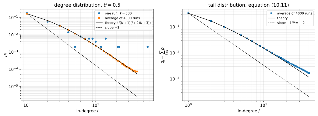
Left: \(p_i\) versus \(i\) on log–log axes for the single required 500-step run (circles) and an average of 4000 runs (squares), against the exact solution \(4/((i+1)(i+2)(i+3))\) of the balance equation (10.8) and the asymptotic slope \(-3\). Right: the tail distribution \(q_j\), whose asymptotic slope is \(-1/\theta=-2\) per equation (10.11).
The ensemble histogram reproduces the closed form to four decimals (\(0.16666\) against \(0.16667\) at \(i=1\), \(0.06663\) against \(0.06667\) at \(i=2\), and on through \(i=8\)) with mean in-degree \(1.0000\), so the growth process and the mean-field difference equation agree.
Fitting a line to the simulated \(p_i\) over the measurable range, however, gives \(-1.86\) for the single run (\(i=1\) to \(8\)) and \(-2.17\) for the ensemble (\(i=1\) to \(20\)), neither near \(-3\). Fitting the exact theoretical \(p_i\) over the same ranges gives \(-1.81\) and \(-2.15\), so the whole discrepancy is the pre-asymptotic bend in \(\prod_k \frac{k}{k+3}\) rather than noise. The exact local slope is \[ \frac{d\log p_i}{d\log i}=-\left(\frac{i}{i+1}+\frac{i}{i+2}+\frac{i}{i+3}\right), \] which is \(-1.08\) at \(i=1\), still \(-2.17\) at \(i=5\) and \(-2.51\) at \(i=10\), reaching \(-2.96\) only near \(i\approx 50\)–\(500\). Equation (10.10) comes from the asymptote (10.9), valid for large \(i\), and \(500\) steps do not populate such degrees; seeing \(-3\) needs \(10^5\)–\(10^6\) nodes. Reading the exponent off a \(500\)-node log–log plot would thus report about \(1.9\) where the generative exponent is \(3\) – an error comparable to the spread among reported Internet exponents, which is the chapter’s point about incomplete measurement.
Problem 10.4 — Backup routing topology design
Backup routing topology design. Consider the topology in Figure 10.10. Nodes \(a\), \(b\), and \(c\) are end hosts and nodes \(A\), \(B\), \(C\), and \(D\) are routers.
Figure 10.10 shows a network with 4 routers \(A\), \(B\), \(C\), \(D\) and 3 end hosts \(a\), \(b\), \(c\), with the following 11 links. Host \(c\) sits at the top and attaches to routers \(A\) and \(B\). Host \(a\) sits on the left and attaches to routers \(A\) and \(C\). Host \(b\) sits at the bottom and attaches to routers \(C\) and \(D\). Among the routers there are five links: \(A\)–\(B\), \(A\)–\(C\), \(B\)–\(C\), \(B\)–\(D\), and \(C\)–\(D\). In full, the edge set is \[ \{a\!-\!A,\;a\!-\!C,\;c\!-\!A,\;c\!-\!B,\;b\!-\!C,\;b\!-\!D,\;A\!-\!B,\;A\!-\!C,\;B\!-\!C,\;B\!-\!D,\;C\!-\!D\}. \]
Each link is 10 Mbps. There are two sessions going on: node \(a\) sends to node \(c\), and node \(b\) sends to node \(c\). Each session can split traffic across multiple paths. A link’s bandwidth is shared equally between the two sessions if they happen to go through the same link.
(a) For a fixed source and destination, node-disjoint paths are paths that do not share any nodes. How many node-disjoint paths are there between \(a\) and \(c\)? Between \(b\) and \(c\)? If \(a\) and \(b\) split their traffic evenly across their disjoint paths, how much bandwidth are \(a\) and \(b\) able to send to \(c\) concurrently?
(b) If router \(A\) fails, what happens? Repeat (a).
(c) If routers \(A\) and \(B\) both fail, what happens? Repeat (a). (difficulty: \(\star\star\))
Two node-disjoint paths per session carrying \(10+10=20\) Mbps with no failure; one path each carrying \(5+5=10\) Mbps when \(A\) fails; and nothing at all when \(A\) and \(B\) both fail, since they are \(c\)’s only neighbours.
(a) Host \(a\) has exactly the two neighbours \(A\) and \(C\), so there are at most two node-disjoint paths to \(c\), and likewise for \(b\); two is achieved, uniquely in each case:
- \(a\to c\): \(\;a\!-\!A\!-\!c\;\) and \(\;a\!-\!C\!-\!B\!-\!c\). (The only alternative first hops are \(A\) and \(C\); from \(C\), reaching \(c\) requires \(A\) or \(B\), since those are \(c\)’s only neighbours, and \(A\) is already used, forcing \(B\).)
- \(b\to c\): \(\;b\!-\!C\!-\!A\!-\!c\;\) and \(\;b\!-\!D\!-\!B\!-\!c\). (From \(D\) the only way to \(c\) avoiding \(C\) is via \(B\); the \(C\)-path must then avoid \(B\), forcing \(A\).)
Each session puts half its rate on each path, so with \(x_a,x_b\) the total session rates the link loads are:
| link | carries |
|---|---|
| \(a\!-\!A\), \(a\!-\!C\), \(C\!-\!B\) | \(x_a/2\) (session \(a\) only) |
| \(b\!-\!C\), \(C\!-\!A\), \(b\!-\!D\), \(D\!-\!B\) | \(x_b/2\) (session \(b\) only) |
| \(A\!-\!c\) | \(x_a/2\) from \(a\) and \(x_b/2\) from \(b\) |
| \(B\!-\!c\) | \(x_a/2\) from \(a\) and \(x_b/2\) from \(b\) |
Only the two last-hop links into \(c\) are shared, and on a shared link each session gets \(10/2=5\) Mbps. So \(x_a/2\le 5\) and \(x_b/2\le 5\), while the unshared links only require \(x/2\le 10\). Therefore
\[ x_a=x_b=10\ \text{Mbps},\qquad \text{total}=20\ \text{Mbps}. \]
Both sessions run at full link speed, and the binding constraint is \(c\)’s own ingress: two 10 Mbps attachments, all of it delivered.
(b) Removing \(A\) leaves \(a\) with the single neighbour \(C\) and \(c\) with the single neighbour \(B\), so every path of either session runs through \(B\) and the link \(B\!-\!c\):
\[ \text{node-disjoint paths } a\to c:\;1\quad (a\!-\!C\!-\!B\!-\!c),\qquad b\to c:\;1\quad (b\!-\!C\!-\!B\!-\!c). \]
With nothing to split across, both sessions share \(B\!-\!c\) and take \(5\) Mbps each:
\[ x_a=x_b=5\ \text{Mbps},\qquad \text{total}=10\ \text{Mbps}. \]
Nothing is disconnected, but throughput halves and the lost diversity means a second failure on \(C\) or \(B\) now cuts a session entirely – graceful degradation, Section 10.2.2’s “many layers of protection”.
(c) Since \(A\) and \(B\) are \(c\)’s only neighbours, removing both isolates it:
\[ \text{node-disjoint paths}: 0 \text{ for both sessions},\qquad x_a=x_b=0,\qquad \text{total}=0\ \text{Mbps}. \]
The rest of the network is untouched, \(a, b, C, D\) staying connected: this is the isolation of one dual-homed edge host, not a global partition, and by Menger’s theorem it was guaranteed the moment (a) produced only two node-disjoint paths.
The code below enumerates node-disjoint paths, applies the even-split-plus-equal-share rule, and separately solves a linear program for the maximum concurrent flow under arbitrary routing as an upper bound; the two agree in every scenario, so the prescribed routing is optimal and not merely feasible.
import networkx as nx, itertools, numpy as np
from scipy.optimize import linprog

E = [('a','A'),('a','C'),('c','A'),('c','B'),('b','C'),('b','D'),
     ('A','B'),('A','C'),('B','C'),('B','D'),('C','D')]
CAP = 10.0

def build(dead=()):
    G = nx.Graph()
    G.add_edges_from([e for e in E if e[0] not in dead and e[1] not in dead])
    return G

def disjoint(G, s, t):
    if s not in G or t not in G or not nx.has_path(G, s, t): return []
    return [list(p) for p in nx.node_disjoint_paths(G, s, t)]

def rates(G, paths):
    # even split across each session's node-disjoint paths; a link is shared
    # equally between the sessions that traverse it
    users = {}
    for s, P in paths.items():
        for p in P:
            for e in zip(p[:-1], p[1:]):
                users.setdefault(frozenset(e), set()).add(s)
    out = {}
    for s, P in paths.items():
        if not P: out[s] = 0.0; continue
        cap = np.inf
        for e, U in users.items():
            k = sum(1 for p in P if e in [frozenset(x) for x in zip(p[:-1], p[1:])])
            if k: cap = min(cap, (CAP/len(U)) * len(P) / k)
        out[s] = cap
    return out

def maxconcurrent(G):
    # LP upper bound: largest t with both sessions sending t, arbitrary routing
    ok = lambda s, d: s in G and d in G and nx.has_path(G, s, d)
    if not (ok('a','c') and ok('b','c')): return 0.0
    arcs = [(u,v) for u,v in G.edges()] + [(v,u) for u,v in G.edges()]
    sess = [('a','c'), ('b','c')]
    idx = {(k,ar): i for i,(k,ar) in enumerate(itertools.product(range(2), arcs))}
    n = len(idx) + 1                                   # last variable is t
    Aeq, beq = [], []
    for k,(s,d) in enumerate(sess):
        for v in G.nodes():
            if v == d: continue
            row = np.zeros(n)
            for ar in arcs:
                if ar[0] == v: row[idx[(k,ar)]] += 1
                if ar[1] == v: row[idx[(k,ar)]] -= 1
            if v == s: row[-1] = -1
            Aeq.append(row); beq.append(0.0)
    Aub, bub = [], []
    for u,v in G.edges():
        row = np.zeros(n)
        for k in range(2):
            row[idx[(k,(u,v))]] = 1; row[idx[(k,(v,u))]] = 1
        Aub.append(row); bub.append(CAP)
    c = np.zeros(n); c[-1] = -1
    r = linprog(c, A_ub=np.array(Aub), b_ub=bub, A_eq=np.array(Aeq), b_eq=beq,
                bounds=[(0,None)]*n, method='highs')
    return r.x[-1]

scen = [('(a) no failure', ()), ('(b) router A fails', ('A',)),
        ('(c) routers A and B fail', ('A','B')), ('[router C fails]', ('C',))]
tot = {}
for label, dead in scen:
    G = build(dead)
    Pa, Pb = disjoint(G,'a','c'), disjoint(G,'b','c')
    r = rates(G, {'a': Pa, 'b': Pb})
    tot[label] = (r['a'], r['b'])
    print(label)
    print('   node-disjoint a->c: %d  %s' % (len(Pa), ['-'.join(p) for p in Pa]))
    print('   node-disjoint b->c: %d  %s' % (len(Pb), ['-'.join(p) for p in Pb]))
    print('   rates  x_a=%.1f  x_b=%.1f Mbps   total=%.1f | LP max-concurrent bound %.1f each'
          % (r['a'], r['b'], r['a']+r['b'], maxconcurrent(G)))
    print('   router degrees:', {v: G.degree(v) for v in 'ABCD' if v in G})

import matplotlib.pyplot as plt
pos = {'c': (0.35, 1.00), 'A': (0.00, 0.62), 'B': (0.80, 0.62), 'a': (-0.55, 0.28),
       'C': (0.00, 0.05), 'D': (0.80, 0.05), 'b': (0.35, -0.30)}
fig, ax = plt.subplots(1, 4, figsize=(18, 4.6))
for k, (label, dead) in enumerate(scen):
    A_ = ax[k]
    for u, v in E:
        live = u not in dead and v not in dead
        A_.plot(*zip(pos[u], pos[v]), color='0.2' if live else '0.90',
                lw=1.8 if live else 1.0, zorder=1)
    for v in pos:
        if v in 'ABCD':
            fc = '#f2c4c4' if v in dead else '#cfe1f2'
        else:
            fc = 'white'
        A_.scatter(*pos[v], s=620, facecolor=fc, edgecolor='0.25', zorder=2)
        A_.text(pos[v][0], pos[v][1], v, ha='center', va='center', fontsize=11, zorder=3)
    xa, xb = tot[label]
    A_.set_title('%s\n%.0f + %.0f = %.0f Mbps' % (label, xa, xb, xa+xb), fontsize=11)
    A_.set_aspect('equal'); A_.axis('off')
plt.tight_layout()
plt.savefig('nl-ch10-backup-topology.svg', dpi=150, bbox_inches='tight')
(a) no failure
   node-disjoint a->c: 2  ['a-A-c', 'a-C-B-c']
   node-disjoint b->c: 2  ['b-C-A-c', 'b-D-B-c']
   rates  x_a=10.0  x_b=10.0 Mbps   total=20.0 | LP max-concurrent bound 10.0 each
   router degrees: {'A': 4, 'B': 4, 'C': 5, 'D': 3}
(b) router A fails
   node-disjoint a->c: 1  ['a-C-B-c']
   node-disjoint b->c: 1  ['b-C-B-c']
   rates  x_a=5.0  x_b=5.0 Mbps   total=10.0 | LP max-concurrent bound 5.0 each
   router degrees: {'B': 3, 'C': 4, 'D': 3}
(c) routers A and B fail
   node-disjoint a->c: 0  []
   node-disjoint b->c: 0  []
   rates  x_a=0.0  x_b=0.0 Mbps   total=0.0 | LP max-concurrent bound 0.0 each
   router degrees: {'C': 3, 'D': 2}
[router C fails]
   node-disjoint a->c: 1  ['a-A-c']
   node-disjoint b->c: 1  ['b-D-B-c']
   rates  x_a=10.0  x_b=10.0 Mbps   total=20.0 | LP max-concurrent bound 10.0 each
   router degrees: {'A': 3, 'B': 3, 'D': 2}
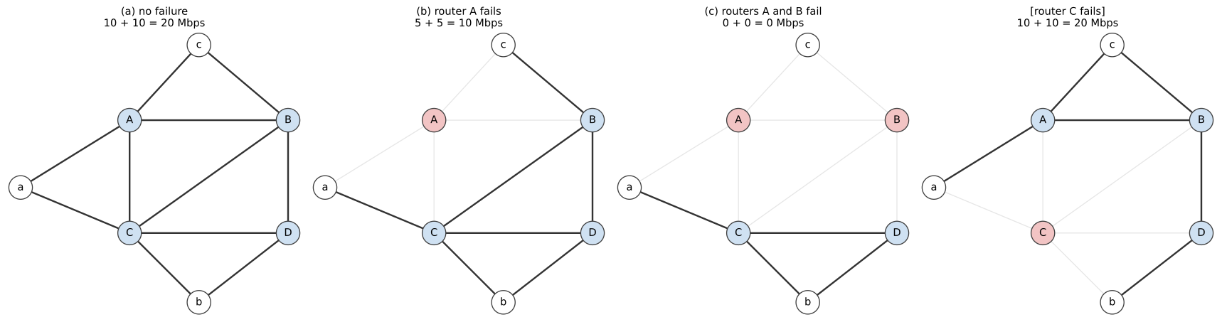
The Figure 10.10 topology under the three required scenarios plus the extra case of losing the highest-degree router \(C\). Blue nodes are live routers, red are failed, white are end hosts; greyed edges are gone. Killing the degree-5 router costs nothing, while killing the degree-4 pair \(\{A,B\}\) isolates host \(c\) entirely.
The output also covers the case the book does not ask for: losing router \(C\) alone, the highest-degree router (degree \(5\) against \(A\) and \(B\)’s \(4\)) and the node an Achilles’-heel argument would target, costs nothing at all, both sessions falling back on the link-disjoint \(a\!-\!A\!-\!c\) and \(b\!-\!D\!-\!B\!-\!c\) for the full \(20\) Mbps. Against router degrees \(\{5,4,4,3\}\):
| attack | routers killed | total throughput |
|---|---|---|
| highest-degree node \(C\) | 1 (degree 5) | 20 Mbps (no loss) |
| node \(A\) | 1 (degree 4) | 10 Mbps (halved) |
| nodes \(A\) and \(B\) | 2 (degree 4 each) | 0 Mbps (\(c\) isolated) |
Degree ranks the wrong nodes. What determines the damage is where the multihoming is: \(c\) buys its resilience from exactly two upstream routers, so the vulnerable set is the cut \(\{A,B\}\), which no reading of the degree sequence reveals. Adding one access link \(c\!-\!C\) or \(c\!-\!D\) would make \(c\) 3-connected and defeat scenario (c) outright, while adding core capacity would not help – robustness bought at the edge, which is Section 10.2.2’s argument in four routers.
Problem 10.5 — Wavelength assignment in optical networks
Wavelength assignment in optical networks. In an optical network for the Internet backbone, each link has a number of wavelengths. An end-to-end path is called a lightpath. A lightpath must be assigned the same wavelength on all of the links along its route. And no two lightpaths can be assigned the same wavelength on any link. For a given graph \(G\) and routing, we want to find an assignment that uses the smallest number of wavelengths subject to these constraints. This is called the wavelength assignment problem.
Figure 10.11 illustrates the problem on an optical ring network. Four nodes \(A\), \(B\), \(C\), \(D\) sit on a ring, joined by the four links \(A\)–\(B\), \(B\)–\(C\), \(C\)–\(D\), \(D\)–\(A\). Two concentric dashed circles run around the ring, drawn just inside and just outside the four nodes; on each of the four links they are labelled \(1\) (inner) and \(2\) (outer). The caption reads: there are two lightpaths, labelled \(1\) and \(2\), on each link between two adjacent nodes.
(a) The well-studied graph-coloring problem asks for the most efficient (using the smallest number of colors) assignment of one color to each node of a graph so that no adjacent nodes have the same color. Show that the wavelength assignment problem on \(G\) is equivalent to the graph coloring problem on a related graph \(\tilde{G}\). What is this \(\tilde{G}\)?
(b) Many optical networks are rings, like in Figure 10.11. There are always two node-disjoint paths between any pair of source-destination nodes to enhance reliability. Let \(L\) be the maximum number of lightpaths on any link. Show that for any set of lightpath requests, at most \(2L-1\) wavelengths are required, by constructing a greedy algorithm of wavelength assignment on a ring. (difficulty: \(\star\star\star\))
(a) \(\tilde G\) is the conflict graph of the routing: one vertex per lightpath \(P_k\), with \(P_k\) adjacent to \(P_\ell\) exactly when \(P_k\cap P_\ell\neq\emptyset\), i.e. when the two share a fibre link of \(G\). The two constraints are what make this a colouring problem: “same wavelength on all links of a route” makes the wavelength a property of a lightpath, so one vertex carries one colour, and “no two lightpaths share a wavelength on a link” is the adjacency condition.
A wavelength assignment is a map \(w:\{P_1,\dots,P_m\}\to\{1,2,\dots\}\), and it is feasible
\begin{equation*} \begin{aligned} &\iff \text{no link carries two lightpaths of one wavelength} \\ &\iff P_k\cap P_\ell\neq\emptyset\Rightarrow w(P_k)\neq w(P_\ell), \end{aligned} \end{equation*}
which is verbatim that \(w\) is a proper vertex colouring of \(\tilde G\). The correspondence is a bijection, not a one-way reduction, so \[ \text{minimum number of wavelengths}\;=\;\chi(\tilde G). \]
Two consequences. A link carrying \(L\) lightpaths makes them pairwise intersecting, hence a clique, so \(\chi(\tilde G)\ge\omega(\tilde G)\ge L\) wavelengths are always needed. And when \(G\) is a line the lightpaths are intervals, \(\tilde G\) is an interval graph, which is perfect, so \(\chi=\omega=L\) and the left-to-right greedy is exactly optimal; on a ring they are circular arcs, \(\tilde G\) is a circular-arc graph, which need not be perfect (\(C_5\) has \(\omega=2\), \(\chi=3\)) and is NP-hard to colour. That is why (b) settles for an approximation.
(b) Label the ring’s links \(e_0,e_1,\dots,e_{n-1}\) in cyclic order. Every lightpath is an arc: a set of consecutive links. Let \(L=\max_k |\{\text{arcs containing } e_k\}|\).
- Pick a link \(e^\star\) of maximum load, so exactly \(L\) arcs contain it. Call that set \(S\). Give the members of \(S\) the distinct wavelengths \(1,2,\dots,L\). (This costs nothing: the arcs of \(S\) pairwise share \(e^\star\), so they form a clique in \(\tilde G\) and must get \(L\) distinct wavelengths in any feasible assignment.)
- Cut the ring open at \(e^\star\). Relabel the remaining links \(f_1,f_2,\dots,f_{n-1}\) in order, walking around the ring away from \(e^\star\). Every arc not in \(S\) is now a contiguous interval \([f_p,f_q]\) on this line. Every arc in \(S\) becomes a prefix \([f_1,f_p]\) and/or a suffix \([f_q,f_{n-1}]\).
- Sort the arcs not in \(S\) by their leftmost link \(f_p\), and sweep left to right. Give each arc the smallest wavelength not already used by any coloured arc that shares a link with it.
The output is feasible by construction, the sweep avoiding every conflicting colour and the first step using \(L\) distinct ones. No wavelength above \(2L-1\) is ever used. Consider the moment the sweep colours some arc \(I=[f_k,f_r]\). Every already-coloured arc that conflicts with \(I\) falls into one of two families, and they are disjoint.
Family (i) is the coloured arcs that contain \(f_k\). It captures every earlier non-\(S\) arc that conflicts with \(I\): such an arc \(J\) has leftmost link index \(\le k\) (it was processed first) and meets \([f_k,f_r]\), so \(J\) must contain \(f_k\). It also captures every \(S\)-arc that meets \(I\) through its prefix piece, since a prefix starts at \(f_1\) and therefore contains \(f_k\) whenever it reaches as far right as \(f_k\). Now the link \(f_k\) carries at most \(L\) arcs in total, and \(I\) is one of them, so
\[ |\text{family (i)}|\;\le\;L-1. \]
Family (ii) is the \(S\)-arcs that meet \(I\) only through their suffix piece \([f_q,f_{n-1}]\), with \(q>k\). Such a piece overlaps \([f_k,f_r]\), so \(q\le r\); and it runs all the way to \(f_{n-1}\), so it contains \(f_r\). Hence every member of family (ii) contains the link \(f_r\) — and so does \(I\). The link \(f_r\) carries at most \(L\) arcs, so
\[ |\text{family (ii)}|\;\le\;L-1. \]
Every coloured arc conflicting with \(I\) is in family (i) or family (ii): if it does not contain \(f_k\) it cannot be an earlier non-\(S\) arc, nor an \(S\)-arc reached through its prefix, so it is an \(S\)-arc reached through its suffix. Therefore at most \((L-1)+(L-1)=2L-2\) wavelengths are blocked when \(I\) is coloured, and the smallest free wavelength is at most \(2L-1\). Since \(I\) was arbitrary, and step 1 used only \(1,\dots,L\le 2L-1\),
\[ \text{the algorithm uses at most } 2L-1 \text{ wavelengths.} \]
Cutting at \(e^\star\) is what turns arcs into intervals and makes “everything earlier that conflicts contains my left endpoint” true; the \(S\)-arcs are the only ones that survive the cut in two pieces, and family (ii) is the price, one extra \(L-1\).
The bound is attained: on a \(5\)-link ring carrying the five arcs \(\{e_0,e_1\},\dots,\{e_4,e_0\}\), every link carries \(2\), so \(L=2\), while \(\tilde G\) is the \(5\)-cycle with \(\chi=3=2L-1\). No algorithm can promise \(2L-2\).
import numpy as np, networkx as nx
from itertools import combinations
import matplotlib.pyplot as plt

def conflict_graph(arcs):
    # G-tilde: one vertex per lightpath, an edge when two lightpaths share a link
    H = nx.Graph(); H.add_nodes_from(range(len(arcs)))
    for i, j in combinations(range(len(arcs)), 2):
        if arcs[i] & arcs[j]: H.add_edge(i, j)
    return H

def load(arcs, n):
    return np.array([sum(1 for a in arcs if k in a) for k in range(n)])

def greedy_ring(arcs, n):
    # cut the ring at a maximum-load link, give the arcs crossing it distinct
    # wavelengths, then sweep the remaining arcs left to right
    ld = load(arcs, n); L = int(ld.max()); estar = int(ld.argmax())
    pos = {(estar + 1 + t) % n: t for t in range(n - 1)}
    colour = {}
    for c, i in enumerate([i for i, a in enumerate(arcs) if estar in a]):
        colour[i] = c
    rest = [i for i in range(len(arcs)) if i not in colour]
    rest.sort(key=lambda i: min(pos[e] for e in arcs[i]))
    for i in rest:
        used = {colour[j] for j in colour if arcs[i] & arcs[j]}
        c = 0
        while c in used: c += 1
        colour[i] = c
    return colour, L

def valid(colour, arcs):
    return all(not (arcs[i] & arcs[j]) or colour[i] != colour[j]
               for i, j in combinations(range(len(arcs)), 2))

def chromatic(H):
    nodes = sorted(H.nodes(), key=lambda v: -H.degree(v))
    for k in range(1, H.number_of_nodes() + 1):
        col = {}
        def bt(t):
            if t == len(nodes): return True
            v = nodes[t]
            for c in range(k):
                if all(col.get(u) != c for u in H[v]):
                    col[v] = c
                    if bt(t + 1): return True
                    del col[v]
            return False
        if bt(0): return k
    return H.number_of_nodes()

print('--- 4-node ring, two lightpaths on every link (Figure 10.11) ---')
arcs4 = [frozenset({0,1}), frozenset({1,2}), frozenset({2,3}), frozenset({3,0})]
col, L = greedy_ring(arcs4, 4)
print('L = %d, bound 2L-1 = %d, greedy uses %d, optimum chi(Gtilde) = %d, valid = %s'
      % (L, 2*L-1, max(col.values())+1, chromatic(conflict_graph(arcs4)), valid(col, arcs4)))

print()
print('--- tightness: 5-link ring, five 2-link arcs ---')
arcs5 = [frozenset({k, (k+1) % 5}) for k in range(5)]
col5, L5 = greedy_ring(arcs5, 5)
H5 = conflict_graph(arcs5)
print('L = %d, bound 2L-1 = %d, greedy uses %d, optimum chi(Gtilde) = %d, Gtilde is C5: %s'
      % (L5, 2*L5-1, max(col5.values())+1, chromatic(H5),
         nx.is_isomorphic(H5, nx.cycle_graph(5))))

print()
print('--- 4000 random ring instances: does greedy ever exceed 2L-1? ---')
rng = np.random.default_rng(5); viol = 0; rows = {}
for _ in range(4000):
    n = int(rng.integers(4, 13)); m = int(rng.integers(2, 26))
    arcs = []
    for _ in range(m):
        s = int(rng.integers(n)); ln = int(rng.integers(1, n))
        arcs.append(frozenset((s + t) % n for t in range(ln)))
    c, L = greedy_ring(arcs, n)
    assert valid(c, arcs)
    W = max(c.values()) + 1
    viol += (W > 2*L - 1)
    rows.setdefault(L, []).append(W)
print('violations of the 2L-1 bound: %d out of 4000' % viol)
print(' L   instances   max wavelengths used   2L-1')
for L in sorted(rows):
    print('%2d   %9d   %20d   %4d' % (L, len(rows[L]), max(rows[L]), 2*L-1))

fig, ax = plt.subplots(1, 2, figsize=(10, 4.4))
th = np.linspace(0, 2*np.pi, 400)
ax[0].plot(np.cos(th), np.sin(th), color='0.85', lw=1)
pal = ['#d1495b', '#2e86ab', '#e9c46a']
for k, a in enumerate(arcs5):
    ks = sorted(a); t0 = 2*np.pi*ks[0]/5; t1 = 2*np.pi*(ks[0]+2)/5
    tt = np.linspace(t0, t1, 100); r = 1.0 + 0.10*(k+1)
    ax[0].plot(r*np.cos(tt), r*np.sin(tt), lw=2.4, color=pal[col5[k]])
    ax[0].text(r*np.cos((t0+t1)/2)*1.06, r*np.sin((t0+t1)/2)*1.06, str(k+1), fontsize=9)
for v in range(5):
    t = 2*np.pi*v/5
    ax[0].plot([np.cos(t)], [np.sin(t)], 'o', ms=9, color='white', mec='0.2')
    ax[0].text(np.cos(t)*0.82, np.sin(t)*0.82, 'v%d' % v, fontsize=8, ha='center')
ax[0].set_aspect('equal'); ax[0].axis('off')
ax[0].set_title('ring $G$: 5 lightpaths, $L=2$ per link', fontsize=10)
p = nx.circular_layout(H5)
nx.draw_networkx_edges(H5, p, ax=ax[1], edge_color='0.4')
nx.draw_networkx_nodes(H5, p, ax=ax[1], node_size=620,
                       node_color=[pal[col5[v]] for v in H5.nodes()], edgecolors='0.2')
nx.draw_networkx_labels(H5, p, {v: str(v+1) for v in H5.nodes()}, ax=ax[1], font_size=10)
ax[1].axis('off')
ax[1].set_title(r'conflict graph $\tilde{G}=C_5$: $\chi=3=2L-1$', fontsize=10)
plt.tight_layout()
plt.savefig('nl-ch10-wavelength-conflict-graph.svg', dpi=150, bbox_inches='tight')
--- 4-node ring, two lightpaths on every link (Figure 10.11) ---
L = 2, bound 2L-1 = 3, greedy uses 2, optimum chi(Gtilde) = 2, valid = True

--- tightness: 5-link ring, five 2-link arcs ---
L = 2, bound 2L-1 = 3, greedy uses 3, optimum chi(Gtilde) = 3, Gtilde is C5: True

--- 4000 random ring instances: does greedy ever exceed 2L-1? ---
violations of the 2L-1 bound: 0 out of 4000
 L   instances   max wavelengths used   2L-1
 1          46                      1      1
 2         220                      3      3
 3         253                      4      5
 4         272                      5      7
 5         258                      7      9
 6         305                      8     11
 7         251                      9     13
 8         254                     11     15
 9         302                     12     17
10         298                     12     19
11         277                     13     21
12         288                     15     23
13         275                     16     25
14         253                     17     27
15         197                     18     29
16         133                     19     31
17          80                     20     33
18          25                     20     35
19           5                     21     37
20           6                     21     39
21           2                     21     41
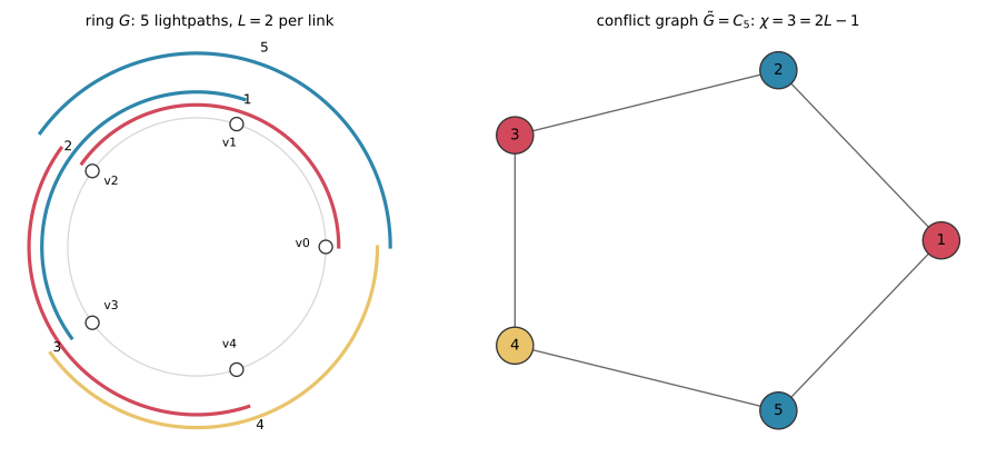
The tight instance. Left: a five-link ring carrying five lightpaths, each spanning two consecutive links, so every link carries \(L=2\); the three colours are the wavelengths the greedy assigns. Right: the conflict graph \(\tilde G\) is the 5-cycle, which needs \(\chi=3=2L-1\) colours. Three wavelengths are unavoidable even though no fibre ever carries more than two lightpaths.
On the Figure 10.11 instance the greedy uses \(2\) wavelengths against a guarantee of \(3\), and on the \(5\)-cycle it uses \(3\), which backtracking confirms is \(\chi(\tilde G)\); across \(4000\) random ring instances the bound is never violated, with a wide margin (at \(L=12\), \(15\) wavelengths against \(23\); at \(L=21\), \(21\) against \(41\)). The factor of two is worst-case pessimism from family (ii). Note that the \(C_5\) example establishes only that \(2L-1\) is attained at \(L=2\), hence that \(L\) itself is unattainable on a ring – not that \(2L-1\) is tight for every \(L\) – and that all of this fixes the routing, the joint routing-and-assignment problem being harder.
Why do AT&T and Verizon Wireless charge me $10 a GB?
Problem 11.1 — Demand elasticity and α-fair utility function
Demand elasticity and \(\alpha\)-fair utility function.
(a) Plot \(\alpha\)-fair utility functions with \(\alpha = 0, \tfrac{1}{5}, \tfrac{1}{2}, 1, 2, 5\), and \(100\) on the same graph, and compare them.
(b) Derive the demand and the demand elasticity as functions of price, if the utility function is \(\arctan(x)\).
(c) Repeat (b) for \(\alpha\)-fairness utility functions. (difficulty: \(\star\))
With \(D(p) = U^{\prime}{}^{-1}(p)\) from \(\max_x U(x) - px\) (Section 11.2.1) and \(\eta(p) = -d\log D/d\log p\), the answers are \(D(p) = \sqrt{(1-p)/p}\), \(\eta(p) = 1/(2(1-p))\) for \(\arctan\), and \(D(p) = p^{-1/\alpha}\), \(\eta \equiv 1/\alpha\) for \(U_\alpha\).
(a) Every member of definition (11.2) has \(U_\alpha^{\prime}(x) = x^{-\alpha} > 0\), so all seven curves are increasing and concave with \(U_\alpha^{\prime}(1) = 1\); only the curvature and the sign change with \(\alpha\).
import numpy as np
import matplotlib.pyplot as plt

def U(x, a):
    if a == 1:
        return np.log(x)
    return x**(1 - a) / (1 - a)

x = np.linspace(0.05, 3.0, 600)
alphas = [0, 0.2, 0.5, 1, 2, 5, 100]
fig, ax = plt.subplots(1, 2, figsize=(11, 4.2))
for a in alphas:
    lab = r'$\alpha=%g$' % a
    ax[0].plot(x, U(x, a), label=lab)
    ax[1].plot(x, U(x, a) - U(1.0, a), label=lab)
ax[0].set_ylim(-6, 4); ax[0].set_title(r'$U_\alpha(x)$ as defined in (11.2)')
ax[1].set_ylim(-6, 4); ax[1].set_title(r'shifted: $U_\alpha(x)-U_\alpha(1)$')
for a_ in ax:
    a_.set_xlabel('x'); a_.axhline(0, lw=0.5, color='k'); a_.grid(alpha=0.3)
    a_.legend(fontsize=8, loc='lower right')
plt.tight_layout()
plt.savefig('nl-ch11-alpha-fair-utilities.svg', dpi=150, bbox_inches='tight')

for a in alphas:
    print('alpha=%6g  U(0.5)=%10.4f  U(1)=%8.4f  U(2)=%9.4f  U(3)=%9.4f' %
          (a, U(0.5, a), U(1.0, a), U(2.0, a), U(3.0, a)))
alpha=     0  U(0.5)=    0.5000  U(1)=  1.0000  U(2)=   2.0000  U(3)=   3.0000
alpha=   0.2  U(0.5)=    0.7179  U(1)=  1.2500  U(2)=   2.1764  U(3)=   3.0103
alpha=   0.5  U(0.5)=    1.4142  U(1)=  2.0000  U(2)=   2.8284  U(3)=   3.4641
alpha=     1  U(0.5)=   -0.6931  U(1)=  0.0000  U(2)=   0.6931  U(3)=   1.0986
alpha=     2  U(0.5)=   -2.0000  U(1)= -1.0000  U(2)=  -0.5000  U(3)=  -0.3333
alpha=     5  U(0.5)=   -4.0000  U(1)= -0.2500  U(2)=  -0.0156  U(3)=  -0.0031
alpha=   100  U(0.5)=-6402275758728431864893145088.0000  U(1)= -0.0101  U(2)=  -0.0000  U(3)=  -0.0000
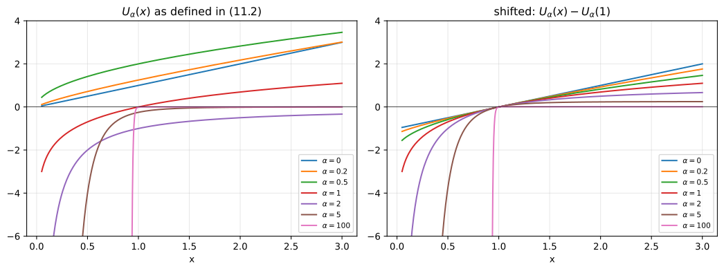
Left: the alpha-fair family exactly as printed in (11.2), for alpha = 0, 1/5, 1/2, 1, 2, 5, 100. Right: the same curves shifted to a common value at x = 1, which is the fair comparison since utilities are only defined up to an additive constant.
Left panel, by regime:
- (i) \(\alpha = 0\): \(U_0(x) = x\) is linear, so \(\max \sum_i x_i\) is pure throughput maximization with no concavity to penalize starving a user (“often unfair”).
- (ii) \(0 < \alpha < 1\): positive, unbounded, concave power laws.
- (iii) \(\alpha = 1\): \(\log x\), unbounded above and unbounded below as \(x \to 0\); that \(-\infty\) penalty is why proportional fairness never assigns a user zero.
- (iv) \(\alpha > 1\): \(U_\alpha(x) = -x^{-(\alpha-1)}/(\alpha-1) < 0\), increasing and bounded above by \(0\), with the punishment at small \(x\) sharpening in \(\alpha\); as \(\alpha \to \infty\) the ordering induced by \(\sum_i U_\alpha(x_i)\) becomes lexicographic in the smallest component, i.e. max-min fairness.
The sign flip at \(\alpha = 1\) is cosmetic: utility is defined only up to an additive constant (which alters neither \(U^{\prime}\) nor the argmax of \(\sum_i U_\alpha(x_i)\)), and the normalization \(\tilde U_\alpha(x) = (x^{1-\alpha}-1)/(1-\alpha)\) of the right panel makes the family continuous in \(\alpha\) with \(\tilde U_1 = \log x\) as the limit. On that scale higher \(\alpha\) bends the curve more sharply, i.e. pulls harder toward equal allocations; \(\alpha = 100\) is visually a step at \(x = 1\).
(b) With \(U(x) = \arctan x\) we have \(U^{\prime}(x) = 1/(1+x^2)\). Setting \(U^{\prime}(x) = p\),
\begin{equation*} 1 + x^2 = \frac{1}{p} \quad \Longrightarrow \quad D(p) = \sqrt{\frac{1-p}{p}}, \qquad 0 < p < 1, \end{equation*}
and \(D(p) = 0\) for \(p \geq 1\), the choke price being \(U^{\prime}(0) = 1\). Taking logs, \(\log D = \tfrac{1}{2}\big(\log(1-p) - \log p\big)\), so
\begin{equation*} \frac{d \log D}{dp} = \frac{1}{2}\left(\frac{-1}{1-p} - \frac{1}{p}\right) = -\frac{1}{2p(1-p)}, \end{equation*}
and therefore
\begin{equation*} \eta(p) = -p\,\frac{d\log D}{dp} = \frac{1}{2(1-p)}. \end{equation*}
This is not constant: \(\eta \to 1/2\) as \(p \to 0\) (bounded utility, near-satiated user), \(\eta \to \infty\) as \(p \to 1^-\), and \(\eta = 1\) at \(p = 1/2\).
(c) For \(U_\alpha\), \(U_\alpha^{\prime}(x) = x^{-\alpha}\) regardless of the \(\alpha \ne 1\) / \(\alpha = 1\) split, so \(x^{-\alpha} = p\) gives
\begin{equation*} D(p) = p^{-1/\alpha}, \qquad \log D = -\frac{1}{\alpha}\log p, \qquad \eta = -\frac{d\log D}{d\log p} = \frac{1}{\alpha}. \end{equation*}
Elasticity is constant in \(p\): this is the isoelastic property quoted in Section 11.2.1 and the axis label “inverse elasticity: \(\alpha\)” of Figure 11.9. Small \(\alpha\) is elastic demand, large \(\alpha\) a captive user; \(\alpha = 1\) recovers the chapter’s \(D(p) = 1/p\), \(\eta = 1\).
Centred finite differences confirm both (Check!):
import numpy as np

D_arctan = lambda p: np.sqrt((1 - p) / p)
eta_arctan = lambda p: 1 / (2 * (1 - p))
D_af = lambda p, a: p**(-1.0 / a)

def eta_numeric(D, p, h=1e-6):
    return -(D(p + h) - D(p - h)) / (2 * h) / (D(p) / p)

print('arctan utility')
for p in [0.05, 0.2, 0.5, 0.8, 0.95]:
    print('  p=%.2f  D=%8.4f  eta_formula=%8.4f  eta_numeric=%8.4f'
          % (p, D_arctan(p), eta_arctan(p), eta_numeric(D_arctan, p)))

print('alpha-fair utility')
for a in [0.5, 1.0, 2.0, 5.0]:
    for p in [0.5, 2.0]:
        print('  alpha=%.1f p=%.1f  D=%8.4f  1/alpha=%6.4f  eta_numeric=%8.4f'
              % (a, p, D_af(p, a), 1 / a, eta_numeric(lambda q: D_af(q, a), p)))
arctan utility
  p=0.05  D=  4.3589  eta_formula=  0.5263  eta_numeric=  0.5263
  p=0.20  D=  2.0000  eta_formula=  0.6250  eta_numeric=  0.6250
  p=0.50  D=  1.0000  eta_formula=  1.0000  eta_numeric=  1.0000
  p=0.80  D=  0.5000  eta_formula=  2.5000  eta_numeric=  2.5000
  p=0.95  D=  0.2294  eta_formula= 10.0000  eta_numeric= 10.0000
alpha-fair utility
  alpha=0.5 p=0.5  D=  4.0000  1/alpha=2.0000  eta_numeric=  2.0000
  alpha=0.5 p=2.0  D=  0.2500  1/alpha=2.0000  eta_numeric=  2.0000
  alpha=1.0 p=0.5  D=  2.0000  1/alpha=1.0000  eta_numeric=  1.0000
  alpha=1.0 p=2.0  D=  0.5000  1/alpha=1.0000  eta_numeric=  1.0000
  alpha=2.0 p=0.5  D=  1.4142  1/alpha=0.5000  eta_numeric=  0.5000
  alpha=2.0 p=2.0  D=  0.7071  1/alpha=0.5000  eta_numeric=  0.5000
  alpha=5.0 p=0.5  D=  1.1487  1/alpha=0.2000  eta_numeric=  0.2000
  alpha=5.0 p=2.0  D=  0.8706  1/alpha=0.2000  eta_numeric=  0.2000
Both formulas match to four decimals.
Problem 11.2 — Optimizing for different utility functions
Optimizing for different utility functions.
Solve the utility maximization problem in the Examples section, but this time with a weighted \(\alpha\)-fair utility function
\begin{equation*} U(x) = \sigma U_\alpha(x) \end{equation*}
where \(\alpha = 0.5\). Then solve it again for \(\alpha = 2\). Compare the results. (difficulty: \(\star\star\))
For the Section 11.3 two-part tariff \(p(x) = g + hx\) with \(U(x) = \sigma U_\alpha(x)\), the demand is \(x^*(h) = (\sigma/h)^{1/\alpha}\) and full extraction of net utility gives the flat-to-usage revenue ratio \(g/(hx^*) = \alpha/(1-\alpha)\) at every \(h\) and \(\sigma\): \(1\) at \(\alpha = 0.5\), and negative (the model breaks) at \(\alpha = 2\).
The printed Example mixes log bases, differentiating \(\sigma\log_{10}x\) as if natural to get \(x^* = \sigma/h\) while evaluating \(g = \sigma(\log_{10}(\sigma/h)-1)\) in base \(10\); nothing here depends on the resolution, since a change of base only rescales \(\sigma\), and the code reproduces the printed \(\$70/\$170\) and \(\$30/\$130\) figures as a setup check.
Demand: \(g\) is constant in \(x\), so the first-order condition for \(\max_x \sigma U_\alpha(x) - g - hx\) is
\begin{equation*} \sigma x^{-\alpha} = h \qquad \Longrightarrow \qquad x^*(h) = \left(\frac{\sigma}{h}\right)^{1/\alpha}, \end{equation*}
the weighted form of \(D(p) = p^{-1/\alpha}\) from Problem 11.1(c), with elasticity \(1/\alpha\). Hence the identity \(h x^* = \sigma (x^*)^{1-\alpha}\), used below. Setting net utility to zero, \(\sigma U_\alpha(x^*) = g + h x^*\), gives
\begin{equation*} g = \frac{\sigma (x^*)^{1-\alpha}}{1-\alpha} - h x^* = h x^*\left(\frac{1}{1-\alpha} - 1\right) = \frac{\alpha}{1-\alpha}\, h x^*. \end{equation*}
so \(g/(hx^*) = \alpha/(1-\alpha)\) independently of \(h\) and \(\sigma\) — the ratio Problem 11.4(b) asks for in the many-flow setting — and total revenue is \(g + hx^* = \sigma(\sigma/h)^{(1-\alpha)/\alpha}/(1-\alpha)\).
(i) \(\alpha = 0.5\) (elastic, \(\eta = 2\)): \(x^* = (\sigma/h)^2\), \(g = hx^*\), so the flat share is \(50\%\) at every \(h\), and total revenue \(2\sigma^2/h \to \infty\) as \(h \to 0\) — the same “make \(h\) arbitrarily small” degeneracy the book flags after its log example, since with no cost and no capacity constraint elastic demand expands faster than the per-unit take shrinks.
(ii) \(\alpha = 2\): the model breaks. Definition (11.2) gives \(U_2(x) = -1/x < 0\), so full extraction demands \(g + hx^* = -\sigma/x^* < 0\), i.e. \(\alpha/(1-\alpha) = -2\): a flat fee of minus twice the usage revenue. The algebra is sound; the assumption that the ISP can extract the full gross utility fails, because a user with everywhere-negative utility buys nothing at any positive price. Hence Figure 11.9 sweeps only \(\alpha \in (0,1)\).
The repair is the additive constant of Problem 11.1(a): \(\tilde U_\alpha(x) = (x^{1-\alpha}-1)/(1-\alpha)\) has the same \(U^{\prime}\) (hence the same \(x^*\) and the same fairness ordering) but \(\tilde U_\alpha(1) = 0\), and \(\tilde U_2(x) = 1 - 1/x \in [0,1)\) for \(x \ge 1\). Then
\begin{equation*} g = \sigma\left(1 - \frac{2}{x^*}\right), \qquad x^* = \sqrt{\sigma/h}, \qquad g + hx^* = \sigma\left(1 - \frac{1}{x^*}\right), \end{equation*}
which is non-negative as soon as \(x^* \geq 2\), i.e. \(h \leq \sigma/4\).
import numpy as np
from scipy.optimize import minimize_scalar

sigma = 100.0

def report(alpha, h, shifted):
    xs = (sigma / h)**(1.0 / alpha)                 # demand: sigma x^-alpha = h
    U = (xs**(1 - alpha) - (1.0 if shifted else 0.0)) / (1 - alpha)
    total = sigma * U                               # full net-utility extraction
    RS = h * xs
    g = total - RS
    return xs, g, RS, total, g / total

print('alpha = 0.5, raw U_alpha (book definition 11.2)')
for h in [2.0, 5.0, 10.0]:
    xs, g, RS, tot, frac = report(0.5, h, False)
    print('  h=%5.1f  x*=%9.2f  g=%9.2f  h x*=%9.2f  total=%9.2f  flat share=%5.1f%%  g/(h x*)=%6.3f'
          % (h, xs, g, RS, tot, 100 * frac, g / RS))

print('alpha = 2, raw U_alpha (book definition 11.2)')
for h in [2.0, 5.0, 10.0]:
    xs, g, RS, tot, frac = report(2.0, h, False)
    print('  h=%5.1f  x*=%9.4f  g=%9.2f  h x*=%9.2f  total=%9.2f  g/(h x*)=%6.3f'
          % (h, xs, g, RS, tot, g / RS))

print('alpha = 2, shifted U = (x^(1-a)-1)/(1-a)  [nonnegative, U(1)=0]')
for h in [2.0, 5.0, 10.0, 0.01]:
    xs, g, RS, tot, frac = report(2.0, h, True)
    print('  h=%5.2f  x*=%9.4f  g=%9.2f  h x*=%9.2f  total=%9.2f  flat share=%5.1f%%  g/(h x*)=%7.3f'
          % (h, xs, g, RS, tot, 100 * frac, g / RS))

print('book base-10 log check (alpha -> 1), sigma = 100')
for h in [2.0, 5.0]:
    xs = sigma / h
    g = sigma * (np.log10(sigma / h) - 1)
    print('  h=%5.1f  x*=%7.1f  g=%7.2f  h x*=%7.2f  total=%7.2f  flat share=%5.1f%%'
          % (h, xs, g, h * xs, g + h * xs, 100 * g / (g + h * xs)))

f = lambda x: -(sigma * x**0.5 / 0.5 - 2.0 * x)
r = minimize_scalar(f, bracket=(1, 100, 1e5))
print('numeric argmax of net utility (alpha=0.5, h=2): x* = %.2f  (closed form %.2f)'
      % (r.x, (sigma / 2.0)**2))
alpha = 0.5, raw U_alpha (book definition 11.2)
  h=  2.0  x*=  2500.00  g=  5000.00  h x*=  5000.00  total= 10000.00  flat share= 50.0%  g/(h x*)= 1.000
  h=  5.0  x*=   400.00  g=  2000.00  h x*=  2000.00  total=  4000.00  flat share= 50.0%  g/(h x*)= 1.000
  h= 10.0  x*=   100.00  g=  1000.00  h x*=  1000.00  total=  2000.00  flat share= 50.0%  g/(h x*)= 1.000
alpha = 2, raw U_alpha (book definition 11.2)
  h=  2.0  x*=   7.0711  g=   -28.28  h x*=    14.14  total=   -14.14  g/(h x*)=-2.000
  h=  5.0  x*=   4.4721  g=   -44.72  h x*=    22.36  total=   -22.36  g/(h x*)=-2.000
  h= 10.0  x*=   3.1623  g=   -63.25  h x*=    31.62  total=   -31.62  g/(h x*)=-2.000
alpha = 2, shifted U = (x^(1-a)-1)/(1-a)  [nonnegative, U(1)=0]
  h= 2.00  x*=   7.0711  g=    71.72  h x*=    14.14  total=    85.86  flat share= 83.5%  g/(h x*)=  5.071
  h= 5.00  x*=   4.4721  g=    55.28  h x*=    22.36  total=    77.64  flat share= 71.2%  g/(h x*)=  2.472
  h=10.00  x*=   3.1623  g=    36.75  h x*=    31.62  total=    68.38  flat share= 53.8%  g/(h x*)=  1.162
  h= 0.01  x*= 100.0000  g=    98.00  h x*=     1.00  total=    99.00  flat share= 99.0%  g/(h x*)= 98.000
book base-10 log check (alpha -> 1), sigma = 100
  h=  2.0  x*=   50.0  g=  69.90  h x*= 100.00  total= 169.90  flat share= 41.1%
  h=  5.0  x*=   20.0  g=  30.10  h x*= 100.00  total= 130.10  flat share= 23.1%
numeric argmax of net utility (alpha=0.5, h=2): x* = 2500.00  (closed form 2500.00)
Comparison, all three differences tracing to \(\eta = 1/\alpha\):
- Volume. At \(\sigma = 100\), \(h = \$2\): \(x^* = 2500\) for \(\alpha = 0.5\) against \(7.07\) for \(\alpha = 2\), and a fourfold cut in \(h\) multiplies \(x^*\) by \(16\) versus \(2\).
- Composition. The flat share is pinned at \(50\%\) for \(\alpha = 0.5\) but rises from \(83.5\%\) toward \(100\%\) as \(h \to 0\) for \(\alpha = 2\) — Figure 11.9 from the single-user side, because the flat fee harvests consumer surplus and an inelastic user’s surplus is almost all inframarginal.
- Is lower \(h\) always better? For \(\alpha = 0.5\), yes and unboundedly so. For \(\alpha = 2\) the utility is bounded, so \(g + hx^* = \sigma(1-1/x^*) \to \$100\) as \(h \to 0\) (the \(h = 0.01\) row gives \(\$99\)): willingness to pay, not the price schedule, caps revenue, and the degeneracy disappears.
Problem 11.3 — Demand vs. supply curves
Demand vs. supply curves.
In general, the demand \(D(p)\) and supply \(S(p)\) as a function of price \(p\) can be defined as follows:
\begin{equation*} D(p) = {U^{\prime}}^{-1}(p), \qquad S(p) = {C^{\prime}}^{-1}(p), \end{equation*}
where \(U(x)\) is the utility of the buyer as a function of the amount purchased and \(C(x)\) is the cost of the producer as a function of the amount produced. Figure 11.10 gives an illustration, with capital letters indicating the sizes of the corresponding areas.
Figure 11.10 is drawn with the quantity \(x\) on the vertical axis and the price \(p\) on the horizontal axis. The demand curve \(D(p)\) starts high on the \(x\)-axis and slopes down to the right, meeting the \(p\)-axis; the supply curve \(S(p)\) starts from a point on the \(p\)-axis just to the right of the origin and slopes up to the right; the two cross once. A dashed horizontal line at height \(x_0\) and a dashed vertical line at \(p_0\) meet on the demand curve, so \(x_0 = D(p_0)\), at a point below and to the right of the crossing. The five labelled areas are: \(C\), bounded by the vertical axis, the \(x_0\) line and the supply curve (below \(x_0\), left of \(S\)); \(B\), below \(x_0\), right of the supply curve and left of \(p_0\); \(A\), below the demand curve and right of \(p_0\); \(D\), above \(x_0\) and left of the supply curve; and \(E\), the sliver above \(x_0\) between the supply and demand curves, up to their crossing.
(a) Assume \(U(0) = 0\), show that \(U(x_0) = A + B + C\). Therefore, the buyer’s net utility is \(U(x_0) - p_0 x_0 = A\).
(b) Assume \(C(0) = 0\), show that \(C(x_0) = C\). Therefore, the seller’s profit is \(p_0 x_0 - C(x_0) = B\).
(c) Let \(x^* = \min\{D(p^*), S(p^*)\}\). At which price \(p^*\) does the social welfare, defined here as \(U(x^*) - C(x^*)\), take the maximum value? (difficulty: \(\star\star\))
Because Figure 11.10 plots quantity vertically against price horizontally, the horizontal distance from the vertical axis to the demand curve at height \(x\) is \(D^{-1}(x) = U^{\prime}(x)\), and to the supply curve is \(S^{-1}(x) = C^{\prime}(x)\); so area swept horizontally as \(x\) runs upward from \(0\) is exactly \(\int U^{\prime}\) or \(\int C^{\prime}\). Everything follows.
(a) By the fundamental theorem of calculus and \(U(0)=0\),
\begin{equation*} U(x_0) = \int_0^{x_0} U^{\prime}(x)\,dx = \int_0^{x_0} D^{-1}(x)\,dx, \end{equation*}
the area between the vertical axis and the demand curve for \(0 \le x \le x_0\). Since \(x_0 = D(p_0)\), the demand curve passes through \((p_0,x_0)\), splitting that area into the rectangle \([0,p_0]\times[0,x_0]\), which the supply curve cuts into \(C\) and \(B\), and the piece to its right, which is \(A\). Hence \(U(x_0) = A + B + C\), while the rectangle’s area is \(p_0x_0 = B + C\); subtracting gives \(U(x_0) - p_0x_0 = A\), the consumer surplus.
(b) Identically, with \(C(0)=0\),
\begin{equation*} C(x_0) = \int_0^{x_0} C^{\prime}(x)\,dx = \int_0^{x_0} S^{-1}(x)\,dx, \end{equation*}
the area between the vertical axis and the supply curve for \(0 \le x \le x_0\), which is region \(C\). Hence the producer surplus is
\begin{equation*} p_0 x_0 - C(x_0) = (B + C) - C = B. \end{equation*}
(c) The welfare-maximizing price is the market-clearing \(p^*\) where the curves cross, \(D(p^*) = S(p^*)\). Writing \(W(x) = U(x) - C(x)\),
\begin{equation*} W^{\prime}(x) = U^{\prime}(x) - C^{\prime}(x) = D^{-1}(x) - S^{-1}(x), \end{equation*}
which by concavity of \(U\) and convexity of \(C\) is positive for \(x < x_e\) and negative for \(x > x_e\), \(x_e\) the crossing quantity; so \(W\) is single-peaked at \(x_e\). And \(x^* = \min\{D(p),S(p)\}\) equals \(S(p)\) for \(p < p_e\) and \(D(p)\) for \(p > p_e\), so \(p \mapsto x^*(p)\) has range \([0,x_e]\), on all of which \(W\) is increasing. The best reachable quantity is thus \(x_e\), attained only at \(p_e\), where \(U^{\prime}(x^*) = C^{\prime}(x^*) = p^*\). In the figure’s letters the maximum welfare is \(A + B + E\), so \(E\) is the deadweight loss from charging \(p_0 > p^*\).
Confirmation with \(D(p) = 10-p\), \(S(p) = p\), so \(U(x) = 10x - x^2/2\), \(C(x) = x^2/2\), at \(p_0 = 7\) (hence \(x_0 = 3\)):
import numpy as np
from scipy.integrate import quad

a, b, c = 10.0, 1.0, 1.0          # D(p) = a - b p,  S(p) = c p
D = lambda p: np.maximum(a - b * p, 0.0)
S = lambda p: c * p
Uprime = lambda x: (a - x) / b     # = D^{-1}(x)
Cprime = lambda x: x / c           # = S^{-1}(x)
U = lambda x: quad(Uprime, 0, x)[0]
C = lambda x: quad(Cprime, 0, x)[0]

p0 = 7.0
x0 = D(p0)
A = quad(D, p0, a / b)[0]                       # right of p0, under D
areaC = quad(Cprime, 0, x0)[0]                  # left of S curve, below x0
B = p0 * x0 - areaC
print('p0 = %.1f, x0 = D(p0) = %.1f' % (p0, x0))
print('A = %.3f   B = %.3f   C = %.3f   A+B+C = %.3f   U(x0) = %.3f'
      % (A, B, areaC, A + B + areaC, U(x0)))
print('buyer net utility U(x0) - p0 x0 = %.3f   (A = %.3f)' % (U(x0) - p0 * x0, A))
print('C(x0) = %.3f  (area C = %.3f);  seller profit p0 x0 - C(x0) = %.3f  (B = %.3f)'
      % (C(x0), areaC, p0 * x0 - C(x0), B))

pe = a / (b + c)
print('market-clearing price p_e = %.4f, quantity x_e = %.4f' % (pe, D(pe)))
best = max(np.linspace(0.01, a / b, 20001),
           key=lambda p: U(min(D(p), S(p))) - C(min(D(p), S(p))))
xs = min(D(best), S(best))
print('grid search over p of U(x*)-C(x*):  p* = %.4f  x* = %.4f  welfare = %.4f'
      % (best, xs, U(xs) - C(xs)))
E = quad(lambda x: Uprime(x) - Cprime(x), x0, D(pe))[0]
print('area E (between the curves, from x0 up to x_e) = %.3f ; A+B+E = %.3f' % (E, A + B + E))
for p in [3.0, 4.0, 5.0, 6.0, 7.0]:
    x = min(D(p), S(p))
    print('   p=%4.1f  x*=min(D,S)=%6.3f  welfare U-C = %8.4f' % (p, x, U(x) - C(x)))
p0 = 7.0, x0 = D(p0) = 3.0
A = 4.500   B = 16.500   C = 4.500   A+B+C = 25.500   U(x0) = 25.500
buyer net utility U(x0) - p0 x0 = 4.500   (A = 4.500)
C(x0) = 4.500  (area C = 4.500);  seller profit p0 x0 - C(x0) = 16.500  (B = 16.500)
market-clearing price p_e = 5.0000, quantity x_e = 5.0000
grid search over p of U(x*)-C(x*):  p* = 5.0000  x* = 5.0000  welfare = 25.0000
area E (between the curves, from x0 up to x_e) = 4.000 ; A+B+E = 25.000
   p= 3.0  x*=min(D,S)= 3.000  welfare U-C =  21.0000
   p= 4.0  x*=min(D,S)= 4.000  welfare U-C =  24.0000
   p= 5.0  x*=min(D,S)= 5.000  welfare U-C =  25.0000
   p= 6.0  x*=min(D,S)= 4.000  welfare U-C =  24.0000
   p= 7.0  x*=min(D,S)= 3.000  welfare U-C =  21.0000
All three claims check: \(A+B+C = U(x_0) = 25.5\), \(C = C(x_0) = 4.5\), and the grid search peaks at \(p^* = 5\) with welfare \(25 = A+B+E\), against \(A+B = 21\) at \(p_0 = 7\).
Problem 11.4 — Flat component vs. usage component
Flat component vs. usage component.
As in the Advanced Material, the simplified revenue-maximization problem for the monopoly ISP is
\begin{equation*} \begin{array}{ll} \text{maximize} & \sum_{t,f} \sigma_f^t U_f\big(D_f^t(h_f^t)\big)\\ \text{subject to} & \sum_f D_f^t(h_f^t) \le C, \quad \forall t\\ \text{variables} & \{h_f^t\}. \end{array} \tag{11.6} \end{equation*}
Let \(h_f^{t*}\) be the usage price that solves the above maximization problem. The resulting volume of consumption is
\begin{equation*} x_f^{t*} = D_f^t(h_f^{t*}), \end{equation*}
and the flat-rate price is
\begin{equation*} g_f^{t*} = \sigma_f^t U_f\big(D_f^t(h_f^{t*})\big) - h_f^{t*} x_f^{t*}. \end{equation*}
(a) Define \(R_F^* = \sum_{t,f} g_f^{t*}\) as the revenue from the flat-rate component and \(R_S^* = \sum_{t,f} h_f^{t*} x_f^{t*}\) as the revenue from the usage component. Prove that
\begin{equation*} \frac{R_F^*}{R_S^*} = \frac{\sum_{f,t}\sigma_f^t U_f(x_f^{t*})}{\sum_{t,f}\sigma_f^t U_f^{\prime}(x_f^{t*})\,x_f^{t*}} - 1. \end{equation*}
(Hint: use \(\sigma_f^t U_f^{\prime}\big(D_f^t(h_f^t)\big) = h_f^t\).)
(b) Show that if \(U_f(x)\) is an \(\alpha\)-fair utility function (\(\alpha \ne 1\)) for all flows \(f\), we have a simpler expression:
\begin{equation*} \frac{R_F^*}{R_S^*} = \frac{\alpha}{1-\alpha}. \end{equation*}
(c) Argue that \(h_f^{t*} = h^{t*}\), i.e., the optimal price per unit of usage is independent of the flow \(f\). (For this part you may want to wait till you have seen Lagrange duality in the Advanced Material in the next chapter.) (difficulty: \(\star\star\star\))
(a) Summing the defining identity \(g_f^{t*} + h_f^{t*}x_f^{t*} = \sigma_f^t U_f(x_f^{t*})\) over \(t,f\) gives \(R_F^* + R_S^* = \sum_{t,f}\sigma_f^t U_f(x_f^{t*})\), so
\begin{equation*} \frac{R_F^*}{R_S^*} = \frac{\sum_{t,f}\sigma_f^t U_f(x_f^{t*})}{R_S^*} - 1, \end{equation*}
and the hint identifies the denominator: since \(D_f^t(h) = U_f^{\prime}{}^{-1}(h/\sigma_f^t)\), inverting at \(x_f^{t*} = D_f^t(h_f^{t*})\) returns \(h_f^{t*} = \sigma_f^t U_f^{\prime}(x_f^{t*})\) (the consumer’s first-order condition for \(\max_x \sigma_f^t U_f(x) - g_f^t - h_f^t x\)), whence
\begin{equation*} R_S^* = \sum_{t,f} h_f^{t*} x_f^{t*} = \sum_{t,f}\sigma_f^t U_f^{\prime}(x_f^{t*})\, x_f^{t*}. \qquad \blacksquare \end{equation*}
Concavity with \(U_f(0) \ge 0\) gives \(U_f(x) \ge U_f^{\prime}(x)x\), so \(R_F^* \ge 0\): the flat fee harvests the inframarginal surplus, area \(A/(B+C)\) of Problem 11.3 aggregated over flows.
(b) For \(U_\alpha(x) = x^{1-\alpha}/(1-\alpha)\) with \(\alpha \ne 1\), \(U_\alpha^{\prime}(x) = x^{-\alpha}\), so
\begin{equation*} U_\alpha^{\prime}(x)\,x = x^{1-\alpha} = (1-\alpha)\,U_\alpha(x), \end{equation*}
Euler’s identity with the same constant \(1-\alpha\) for every flow and slot. Hence, term by term,
\begin{equation*} \sum_{t,f}\sigma_f^t U_\alpha^{\prime}(x_f^{t*})\,x_f^{t*} = (1-\alpha)\sum_{t,f}\sigma_f^t U_\alpha(x_f^{t*}), \end{equation*}
so the ratio in (a) collapses independently of \(\{\sigma_f^t\}\), of \(C\), and of the optimizer:
\begin{equation*} \frac{R_F^*}{R_S^*} = \frac{1}{1-\alpha} - 1 = \frac{\alpha}{1-\alpha}. \qquad \blacksquare \end{equation*}
The exclusion \(\alpha \ne 1\) is not removable: \(U_1^{\prime}(x)x \equiv 1\) while \(U_1 = \log x\) is not constant, so the ratio then depends on the allocation; \(\alpha/(1-\alpha) \to \infty\) as \(\alpha \to 1^-\) is the chapter’s statement that flat revenue dominates for log utilities. Meaning also requires \(\alpha < 1\), for the reason diagnosed in Problem 11.2.
(c) Strict concavity of \(U_f\) makes \(D_f^t(h) = U_f^{\prime}{}^{-1}(h/\sigma_f^t)\) a decreasing bijection, so optimizing over \(\{h_f^t\}\) is optimizing over the induced \(\{x_f^t\}\), and (11.6) becomes
\begin{equation*} \begin{array}{ll} \text{maximize} & \sum_t \sum_f \sigma_f^t U_f(x_f^t)\\ \text{subject to} & \sum_f x_f^t \le C, \quad \forall t, \end{array} \end{equation*}
a concave maximization decoupling across time slots, with Slater’s condition met (\(C > 0\)), so KKT is necessary and sufficient. With multiplier \(\lambda^t \ge 0\) on the time-\(t\) constraint,
\begin{equation*} L = \sum_f \sigma_f^t U_f(x_f^t) - \lambda^t\Big(\sum_f x_f^t - C\Big), \end{equation*}
stationarity in \(x_f^t\) gives, for every flow with \(x_f^{t*} > 0\),
\begin{equation*} \sigma_f^t U_f^{\prime}(x_f^{t*}) = \lambda^t . \end{equation*}
whose left-hand side is the price \(h_f^{t*}\) by the hint of (a). Hence \(h_f^{t*} = \lambda^t =: h^{t*}\) for every \(f\): the optimal usage price is the shadow price of capacity in that slot, a property of the congested resource and not of the customer. Equivalently, without the Lagrangian, if \(\sigma_1^t U_1^{\prime}(x_1^t) > \sigma_2^t U_2^{\prime}(x_2^t)\) then moving \(\epsilon\) of capacity from flow \(2\) to flow \(1\) leaves the constraint intact and raises the objective by \(\epsilon(\sigma_1^tU_1^{\prime} - \sigma_2^tU_2^{\prime}) > 0\), so the point was not optimal; strict concavity makes the maximizer unique. Note that \(h^{t*}\) must be common across flows for efficiency while \(g_f^{t*}\) stays flow-specific, which is what lets the monopolist price-discriminate on surplus.
Verification of (b) and (c) on ten flows sharing \(C = 10\) Mbps with \(\sigma_f\) uniform on \([1,2]\), where the KKT system water-fills to \(x_f = (\sigma_f/\lambda)^{1/\alpha}\), \(\lambda = (\sum_f \sigma_f^{1/\alpha}/C)^{\alpha}\):
import numpy as np
from scipy.optimize import minimize
import matplotlib.pyplot as plt

rng = np.random.default_rng(11)
F, Cap = 10, 10.0                       # 10 flows, C = 10 Mbps
sig = rng.uniform(1.0, 2.0, F)          # utility levels sigma_f in [sigma_0, sigma_1]

def solve(alpha):
    lam = (np.sum(sig**(1 / alpha)) / Cap)**alpha    # water-filling multiplier
    x = (sig / lam)**(1 / alpha)
    return lam, x

print('KKT check: is sigma_f U_f\'(x_f) the same for every flow?  (alpha = 0.6)')
lam, x = solve(0.6)
h = sig * x**(-0.6)
print('  x_f      =', np.round(x, 4))
print('  h_f      =', np.round(h, 6))
print('  spread of h_f = %.3e ; lambda = %.6f ; sum x_f = %.6f' % (h.max() - h.min(), lam, x.sum()))

alpha = 0.6
obj = lambda z: -np.sum(sig * z**(1 - alpha)) / (1 - alpha)
res = minimize(obj, np.full(F, Cap / F), method='SLSQP',
               bounds=[(1e-6, None)] * F,
               constraints=[{'type': 'eq', 'fun': lambda z: z.sum() - Cap}])
print('  SLSQP optimum matches closed form to %.2e' % np.abs(res.x - x).max())
hn = sig * res.x**(-alpha)
print('  h_f from SLSQP: min %.6f  max %.6f' % (hn.min(), hn.max()))

print()
print('revenue split, and comparison with alpha/(1-alpha)')
print(' alpha    h*=lambda     R_S       R_F      total    R_F/R_S   alpha/(1-alpha)')
for a in [0.1, 0.25, 0.5, 0.6, 0.75, 0.9, 0.95]:
    lam, x = solve(a)
    RS = lam * Cap
    RF = np.sum(sig * x**(1 - a)) / (1 - a) - RS
    print(' %5.2f  %9.4f %9.4f %9.4f %9.4f %9.4f %9.4f'
          % (a, lam, RS, RF, RS + RF, RF / RS, a / (1 - a)))

lam, x = solve(0.6)
best = np.sum(sig * x**0.4) / 0.4
worse = []
for _ in range(5):
    d = rng.normal(0, 0.3, F); d -= d.mean()
    z = np.clip(x + d, 1e-3, None); z *= Cap / z.sum()
    worse.append(np.sum(sig * z**0.4) / 0.4)
print()
print('alpha=0.6 optimal revenue %.5f ; 5 capacity-filling but unequal-h allocations:' % best)
print('  ', np.round(worse, 5))

al = np.linspace(0.02, 0.97, 300)
tot, flat, use = [], [], []
for a in al:
    lam, x = solve(a)
    RS = lam * Cap
    RF = RS * a / (1 - a)
    use.append(RS); flat.append(RF); tot.append(RS + RF)
fig, ax = plt.subplots(2, 1, figsize=(7, 6.5), sharex=True)
ax[0].semilogy(al, tot, 'k-', label='Total')
ax[0].semilogy(al, flat, 'k--', label='Flat')
ax[0].semilogy(al, use, 'k-.', label='Usage')
ax[0].set_ylabel('Revenue ($)'); ax[0].legend(); ax[0].grid(alpha=0.3)
ax[1].plot(al, np.array(flat) / np.array(use), 'k--', lw=3, label='computed $R_F^*/R_S^*$')
ax[1].plot(al, al / (1 - al), 'r:', lw=1.5, label=r'$\alpha/(1-\alpha)$')
ax[1].set_ylim(0, 20); ax[1].set_xlabel(r'inverse elasticity: $\alpha$')
ax[1].set_ylabel('$R_F^*/R_S^*$'); ax[1].legend(); ax[1].grid(alpha=0.3)
plt.tight_layout()
plt.savefig('nl-ch11-flat-usage-split.svg', dpi=150, bbox_inches='tight')
print()
print('max |computed ratio - alpha/(1-alpha)| over the sweep = %.3e'
      % np.abs(np.array(flat) / np.array(use) - al / (1 - al)).max())
KKT check: is sigma_f U_f'(x_f) the same for every flow?  (alpha = 0.6)
  x_f      = [0.6686 1.0734 1.1981 0.5729 0.6878 1.6326 0.6122 0.6698 1.6611 1.2236]
  h_f      = [1.436915 1.436915 1.436915 1.436915 1.436915 1.436915 1.436915 1.436915
 1.436915 1.436915]
  spread of h_f = 2.220e-16 ; lambda = 1.436915 ; sum x_f = 10.000000
  SLSQP optimum matches closed form to 2.62e-04
  h_f from SLSQP: min 1.436724  max 1.437126

revenue split, and comparison with alpha/(1-alpha)
 alpha    h*=lambda     R_S       R_F      total    R_F/R_S   alpha/(1-alpha)
  0.10     1.6815   16.8149    1.8683   18.6833    0.1111    0.1111
  0.25     1.5258   15.2584    5.0861   20.3445    0.3333    0.3333
  0.50     1.4501   14.5013   14.5013   29.0027    1.0000    1.0000
  0.60     1.4369   14.3692   21.5537   35.9229    1.5000    1.5000
  0.75     1.4237   14.2367   42.7101   56.9467    3.0000    3.0000
  0.90     1.4149   14.1485  127.3368  141.4853    9.0000    9.0000
  0.95     1.4125   14.1254  268.3824  282.5078   19.0000   19.0000

alpha=0.6 optimal revenue 35.92288 ; 5 capacity-filling but unequal-h allocations:
   [35.74941 35.7232  35.74995 35.46578 35.61857]

max |computed ratio - alpha/(1-alpha)| over the sweep = 3.553e-15
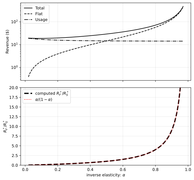
Ten flows sharing C = 10 Mbps with random utility levels. Top (log scale): flat, usage, and total revenue against alpha. Bottom: the computed flat-to-usage ratio lying exactly on alpha/(1-alpha), reproducing the lower panel of Figure 11.9.
The ten prices agree to machine precision though the \(x_f\) differ by a factor of three, an independent SLSQP solve lands on the same point, and every capacity-filling perturbation lowers revenue below \(35.923\) — the concrete form of (c). The computed \(R_F^*/R_S^*\) matches \(\alpha/(1-\alpha)\) to \(3.6\times10^{-15}\). The upper panel reproduces Figure 11.9: \(R_S^* = h^*C\) declines only mildly (\(16.8\) to \(14.1\), since capacity sells out either way and only the shadow price moves) while flat revenue climbs steeply, crossing at \(\alpha = 1/2\).
Problem 11.5 — Braess’ paradox
Braess’ paradox.
Consider a road network as illustrated in Figure 11.11(a), on which 3000 drivers wish to travel from node Start to node End. Denote by \(x\) the number of travelers passing through the link Start \(\to\) A, and by \(y\) the number of travelers passing through the link B \(\to\) End. The travel time of each link in minutes is labeled next to the corresponding link. Suppose everyone chooses her route from Start to End to minimize the total travel time.
Figure 11.11(a) is a diamond with four nodes. From Start there are two outgoing links: Start \(\to\) B with constant travel time \(50\), and Start \(\to\) A with travel time \(10 + x/100\). From those two nodes there are two links into End: B \(\to\) End with travel time \(10 + y/100\), and A \(\to\) End with constant travel time \(50\). Figure 11.11(b) is the same diamond with one extra link added, A \(\to\) B, with constant travel time \(5\).
(a) What is the resulting traffic and the total travel time for each commuter?
(b) Suppose the government built a shortcut from node A and B with travel time labeled as illustrated in Figure 11.11(b). What is the resulting traffic and the total traveling time for each commuter?
(c) This is the famous Braess’ paradox. Suggest a way to avoid it. (difficulty: \(\star\star\star\))
The equilibrium is \(x = y = 1500\) at \(75\) minutes without the shortcut and \(x = y = 3000\) at \(85\) minutes with it; congestion pricing is the fix. Write \(a,b,c\) for the numbers on Start-A-End, Start-B-End and the zigzag Start-A-B-End, so \(x = a+c\), \(y = b+c\), \(a+b+c = 3000\), and
\begin{equation*} T_a = 60 + \tfrac{x}{100}, \qquad T_b = 60 + \tfrac{y}{100}, \qquad T_c = 25 + \tfrac{x}{100} + \tfrac{y}{100}. \end{equation*}
Selfish routing means a Wardrop equilibrium: every used route ties, no unused route is faster.
(a) Here \(c = 0\), \(x = a\), \(y = 3000 - x\), and equating,
\begin{equation*} 60 + \frac{x}{100} = 60 + \frac{3000-x}{100} \quad \Longrightarrow \quad x = 1500, \end{equation*}
an even split, \(T = 60 + 15 = 75\) minutes each and \(225{,}000\) driver-minutes in total. This is also the social optimum, since \(180000 + [x^2 + (3000-x)^2]/100\) is convex and symmetric about \(x = 1500\): selfish routing costs nothing here.
(b) All \(3000\) take the zigzag, so \(x = y = 3000\) and \(T_c = 85\) minutes. It is the only equilibrium: for any split,
\begin{equation*} T_a - T_c = 35 - \frac{y}{100} \ge 5, \qquad T_b - T_c = 35 - \frac{x}{100} \ge 5, \end{equation*}
since \(x,y \le 3000\), so the zigzag strictly dominates and \(a = b = 0\). Every driver is ten minutes worse off and the system total rises to \(255{,}000\) driver-minutes. The mechanism is the negative externality of Section 11.2.2: the new link puts everyone on both congestible links at once, and each driver ignores the \(1/100\) minute she adds for the \(3000\) behind her — private cost \(85\) against marginal social cost \(85 + 3000\cdot\tfrac{2}{100} = 145\).
(c) Toll each congestible link at the externality its users impose. For latency \(\ell(x)\) the marginal social cost of one more driver is \(\ell(x) + x\ell^{\prime}(x)\), of which she already bears \(\ell(x)\), so the toll is
\begin{equation*} \tau = x\,\ell^{\prime}(x). \end{equation*}
with \(\ell^{\prime} = 1/100\) on Start \(\to\) A and B \(\to\) End and \(0\) elsewhere, evaluated at the system optimum.
import numpy as np
from scipy.optimize import minimize

N = 3000.0

def times(a, b, c):
    """a: Start-A-End, b: Start-B-End, c: Start-A-B-End (zigzag).  returns (T_a, T_b, T_c)"""
    x, y = a + c, b + c                      # flow on S->A and on B->End
    return (10 + x / 100 + 50,
            50 + 10 + y / 100,
            10 + x / 100 + 5 + 10 + y / 100)

def total_time(a, b, c):
    Ta, Tb, Tc = times(a, b, c)
    return a * Ta + b * Tb + c * Tc

print('(a) no shortcut: split N between the two routes')
for x in [1000, 1400, 1500, 1600, 2000]:
    Ta, Tb, _ = times(x, N - x, 0.0)
    print('   x=%5d  y=%5d  T(upper)=%6.2f  T(lower)=%6.2f' % (x, N - x, Ta, Tb))
grid = np.arange(0, N + 1)
eq = grid[np.argmin([abs(times(x, N - x, 0)[0] - times(x, N - x, 0)[1]) for x in grid])]
Ta, Tb, _ = times(eq, N - eq, 0)
print('   equilibrium x = %d, travel time = %.2f min, system total = %.0f min'
      % (eq, Ta, total_time(eq, N - eq, 0)))

print()
print('(b) with the 5-minute A->B shortcut, all 3000 on the zigzag')
Ta, Tb, Tc = times(0.0, 0.0, N)
print('   T(Start-A-End) = %.1f   T(Start-B-End) = %.1f   T(zigzag) = %.1f' % (Ta, Tb, Tc))
print('   nobody gains by deviating: %s' % (Tc <= min(Ta, Tb)))
print('   equilibrium travel time = %.2f min, system total = %.0f min' % (Tc, total_time(0, 0, N)))

print('   uniqueness scan over (a,b,c) on a 50-driver grid: any other Wardrop equilibrium?')
bad = []
for a in np.arange(0, N + 1, 50):
    for b in np.arange(0, N - a + 1, 50):
        c = N - a - b
        T = times(a, b, c)
        used = [T[i] for i, fl in enumerate([a, b, c]) if fl > 0]
        if max(used) - min(used) < 1e-9 and min(T) >= min(used) - 1e-9:
            bad.append((a, b, c, round(min(used), 3)))
print('   equilibria found:', bad)

print()
print('(c) social optimum with the shortcut in place')
res = minimize(lambda z: total_time(z[0], z[1], N - z[0] - z[1]),
               [1000., 1000.], method='Nelder-Mead',
               options={'xatol': 1e-8, 'fatol': 1e-10})
a_o, b_o = res.x; c_o = N - a_o - b_o
print('   optimum a=%.2f  b=%.2f  c=%.2f  total=%.2f  average=%.4f min'
      % (a_o, b_o, c_o, res.fun, res.fun / N))
x_o, y_o = a_o + c_o, b_o + c_o
print('   flows: x = %.2f, y = %.2f' % (x_o, y_o))
tau = x_o / 100                              # marginal-cost toll  x * l'(x)  on each variable link
print('   marginal-cost toll on Start->A and on B->End = %.2f' % tau)
Ta, Tb, Tc = times(a_o, b_o, c_o)
print('   toll-inclusive costs:  route a %.2f   route b %.2f   zigzag %.2f'
      % (Ta + tau, Tb + tau, Tc + 2 * tau))
print('   actual travel times :  route a %.2f   route b %.2f   zigzag %.2f' % (Ta, Tb, Tc))
print('   price of anarchy = %.4f   (affine-latency bound 4/3 = %.4f)'
      % (total_time(0, 0, N) / res.fun, 4 / 3))
(a) no shortcut: split N between the two routes
   x= 1000  y= 2000  T(upper)= 70.00  T(lower)= 80.00
   x= 1400  y= 1600  T(upper)= 74.00  T(lower)= 76.00
   x= 1500  y= 1500  T(upper)= 75.00  T(lower)= 75.00
   x= 1600  y= 1400  T(upper)= 76.00  T(lower)= 74.00
   x= 2000  y= 1000  T(upper)= 80.00  T(lower)= 70.00
   equilibrium x = 1500, travel time = 75.00 min, system total = 225000 min

(b) with the 5-minute A->B shortcut, all 3000 on the zigzag
   T(Start-A-End) = 90.0   T(Start-B-End) = 90.0   T(zigzag) = 85.0
   nobody gains by deviating: True
   equilibrium travel time = 85.00 min, system total = 255000 min
   uniqueness scan over (a,b,c) on a 50-driver grid: any other Wardrop equilibrium?
   equilibria found: [(0.0, 0.0, 3000.0, 85.0)]

(c) social optimum with the shortcut in place
   optimum a=1250.00  b=1250.00  c=500.00  total=223750.00  average=74.5833 min
   flows: x = 1750.00, y = 1750.00
   marginal-cost toll on Start->A and on B->End = 17.50
   toll-inclusive costs:  route a 95.00   route b 95.00   zigzag 95.00
   actual travel times :  route a 77.50   route b 77.50   zigzag 60.00
   price of anarchy = 1.1397   (affine-latency bound 4/3 = 1.3333)
The social optimum of the five-link network is \(a = b = 1250\), \(c = 500\), at \(74.58\) minutes: with \(a = b = (3000-c)/2\) and \(x = y = (3000+c)/2\) the system total is \(180000 - 35c + (3000+c)^2/200\), whose derivative \(-35 + (3000+c)/100\) vanishes at \(c = 500\). The toll \(\tau = 1750/100 = 17.50\) on each congestible link makes all three routes cost \(95\) in time plus toll, so the optimum is the tolled equilibrium. Closing the shortcut instead gives \(75\): the road is useful, and what was broken was the absence of a price on it. Doing nothing costs a price of anarchy \(255000/223750 = 1.14\), inside the \(4/3\) worst case for affine latencies (Roughgarden and Tardos).
Central routing is the alternative, assigning \(1250/1250/500\) directly for the same \(74.58\), but it needs compliance and creates the inequity the toll settles with money: the \(500\) zigzag drivers take \(60\) minutes while the other \(2500\) take \(77.5\). Removing links (42nd Street, Seoul’s Cheonggyecheon expressway) works but leaves the \(75\) versus \(74.58\) gap on the table, and corresponds in a data network to caps, throttling, and blocking rather than to pricing.
How can I pay less for each GB?
Problem 12.1 — Time-dependent pricing
Time-dependent pricing. An ISP tries to even out the capacity demand over day and night by rewarding its users for delaying their data transmission. Suppose there are just two types of users, type A and type B, which have different levels of willingness to delay their sessions. Originally the demand during day-time is in total \(v_{A,day} + v_{B,day} = 14\) GB, which consists of \(v_{A,day} = 8\) GB from type A users and \(v_{B,day} = 6\) GB from type B users. The demand during night-time is in total \(v_{A,night} + v_{B,night} = 5\) GB, which consists of \(v_{A,night} = 2\) GB from type A users and \(v_{B,night} = 3\) GB from type B users.
Suppose the ISP has capacity \(C = 10\) GB and the marginal cost of exceeding capacity is $1 per GB. It provides a reward of $\(p\) per GB for day-time users to delay their data transfer until night-time. Let \(w_A(p)\) and \(w_B(p)\) be the proportions of data from type A and type B users, respectively, to be delayed from day-time to night-time:
\[ w_A(p) = 1 - \exp\left(-\frac{p}{p_A}\right), \qquad w_B(p) = 1 - \exp\left(-\frac{p}{p_B}\right), \]
where parameters \(p_A = 4\) and \(p_B = 2\).
The ISP wishes to find the reward price \(p^*\) that minimizes its total cost, i.e., the sum of the cost due to the demand exceeding the capacity and the rewards given out.
(a) What is the formulation of the minimization problem?
(b) Solve \(p^*\) numerically by plotting the objective function over the reward price \(p\). (difficulty: \(\star\star\))
(a) With the reward \(p \ge 0\) as the single variable, the deferred volume is the Section 12.4.1 sum \(\sum_{k\ne i}\sum_{j\in k} v_j w_j\), here
\[ S(p) \;=\; v_{A,day}\,w_A(p) + v_{B,day}\,w_B(p) \;=\; 8\left(1 - e^{-p/4}\right) + 6\left(1 - e^{-p/2}\right), \]
so the usages become \(x_{day} = 14 - S(p)\) and \(x_{night} = 5 + S(p)\) (the reward moves traffic one way only), the reward bill is \(pS(p)\), and with \(C = 10\) and $1 per GB overage charged per period the program is
\[ \underset{p \ge 0}{\text{minimize}} \quad J(p) = p\,S(p) + \max\{0,\, 4 - S(p)\} + \max\{0,\, S(p) - 5\}. \]
Since \(S\) is increasing and concave with \(S(0) = 0\) and \(S^{\prime}(0) = 8/4 + 6/2 = 5\), we get \(J^{\prime}(0) = -5 < 0\), so some reward always pays; and \(S \in [4,5]\) is the zero-overage window, below which the day is congested and above which the night is.
(b) On the branch \(S(p) < 4\) the objective is \(J = pS + 4 - S\), with
\[ J^{\prime}(p) = S(p) + (p-1)S^{\prime}(p) = 0, \qquad S^{\prime}(p) = 2e^{-p/4} + 3e^{-p/2}. \]
A grid search, a bounded scalar minimizer, and that stationarity condition agree.
import numpy as np
from scipy.optimize import minimize_scalar, brentq

vAd, vBd, vAn, vBn, C = 8.0, 6.0, 2.0, 3.0, 10.0
pA, pB = 4.0, 2.0

def S(p):
    return vAd*(1-np.exp(-p/pA)) + vBd*(1-np.exp(-p/pB))

def Sprime(p):
    return (vAd/pA)*np.exp(-p/pA) + (vBd/pB)*np.exp(-p/pB)

def J(p):
    s = S(p)
    return p*s + max(0.0, vAd+vBd-s-C) + max(0.0, vAn+vBn+s-C)

grid = np.linspace(0, 6, 600001)
vals = np.array([J(p) for p in grid])
i = int(np.argmin(vals))
res = minimize_scalar(J, bounds=(0, 6), method='bounded',
                      options={'xatol': 1e-12})
root = brentq(lambda p: S(p) + (p-1)*Sprime(p), 1e-6, 3.0)

print("grid    p* = %.6f  cost = %.6f" % (grid[i], vals[i]))
print("refined p* = %.6f  cost = %.6f" % (res.x, res.fun))
print("stationary point of S + (p-1)S' : %.6f" % root)
print("shifted S(p*) = %.6f GB" % S(res.x))
print("day = %.6f GB, night = %.6f GB" % (14-S(res.x), 5+S(res.x)))
print("no-TDP cost J(0) = %.6f" % J(0.0))
grid    p* = 0.476130  cost = 2.863799
refined p* = 0.476127  cost = 2.863799
stationary point of S + (p-1)S' : 0.476127
shifted S(p*) = 2.168845 GB
day = 11.831155 GB, night = 7.168845 GB
no-TDP cost J(0) = 4.000000
import numpy as np
import matplotlib.pyplot as plt

p = np.linspace(0, 3, 3000)
s = 8*(1-np.exp(-p/4)) + 6*(1-np.exp(-p/2))
j = p*s + np.maximum(0, 4-s) + np.maximum(0, s-5)
i = int(np.argmin(j))

fig, ax = plt.subplots(1, 2, figsize=(11, 4))
ax[0].plot(p, j, lw=2)
ax[0].plot(p[i], j[i], 'o', color='crimson')
ax[0].annotate('$p^*=%.3f$, cost $=\\$%.3f$' % (p[i], j[i]), (p[i], j[i]),
               textcoords='offset points', xytext=(12, 18))
ax[0].set_xlabel('reward $p$ (\\$/GB)')
ax[0].set_ylabel('total cost ($)')
ax[0].set_title('Problem 12.1 objective')
ax[0].grid(alpha=.3)
ax[1].plot(p, 14-s, label='day usage')
ax[1].plot(p, 5+s, label='night usage')
ax[1].axhline(10, ls='--', c='k', label='capacity $C=10$')
ax[1].axvline(p[i], ls=':', c='crimson')
ax[1].set_xlabel('reward $p$ (\\$/GB)')
ax[1].set_ylabel('GB')
ax[1].set_title('usage after shifting')
ax[1].legend()
ax[1].grid(alpha=.3)
plt.tight_layout()
plt.savefig('nl-ch12-tdp-objective.svg', dpi=150, bbox_inches='tight')
print("p* = %.4f, minimum cost = %.4f" % (p[i], j[i]))
p* = 0.4762, minimum cost = 2.8638
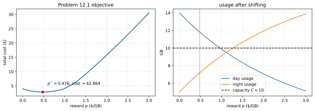
Problem 12.1. Left: total ISP cost (rewards plus capacity overage) as a function of the deferral reward \(p\), minimized at \(p^* \approx \$0.476\)/GB. Right: day-time and night-time usage after shifting; at \(p^*\) the day is still above the 10 GB capacity, so the ISP deliberately stops short of eliminating the overage.
Hence \(p^* \approx \$0.476\) per GB at a total cost of $2.864, against $4.00 with no TDP. The optimum deliberately stops short of clearing the overage: only \(2.17\) GB moves, leaving \(11.83\) GB in the day and $1.83 of overage, because the reward is paid on every shifted GB, so raising \(p\) costs \(S + pS^{\prime}\) at the margin while saving only \(S^{\prime}\). Reaching \(S = 4\) would need \(p \approx 0.96\) and \(\$3.85\) of rewards alone.
Problem 12.2 — User-type estimation
User-type estimation. Consider the same model as in the above problem, except that now the values \(v_{A,day}\), \(v_{B,day}\), \(v_{A,night}\) and \(v_{B,night}\) are unknown. Suppose that originally the demand during daytime is in total 17 GB, and after announcing a reward price of $0.30 per GB the demand during daytime reduces to 15.2 GB in total. What are \(v_{A,day}\) and \(v_{B,day}\)? (difficulty: \(\star\star\))
\(v_{A,day} \approx 8.47\) GB and \(v_{B,day} \approx 8.53\) GB. The trial of Section 12.2.2 gives two linear equations in the two unknowns, the second because day traffic drops by exactly the deferred volume, with \(w_A, w_B\) as in Problem 12.1 (\(p_A = 4\), \(p_B = 2\)) at \(p = 0.30\):
\[ v_{A,day} + v_{B,day} = 17, \qquad w_A(0.3)\,v_{A,day} + w_B(0.3)\,v_{B,day} = 1.8. \]
The night volumes never enter, since the reward moves traffic only out of the day, so only the day volumes are identifiable here. Writing \(z = e^{-0.075}\), so \(w_A = 1-z\) and \(w_B = 1-z^2\), substitution of \(v_{B,day} = 17 - v_{A,day}\) gives
\[ (1-z)v_{A,day} + (1-z^2)(17 - v_{A,day}) = 1.8 \;\Longrightarrow\; v_{A,day}\,(z^2 - z) = 1.8 - 17(1-z^2), \]
hence
\[ v_{A,day} = \frac{17(1-z^2) - 1.8}{z(1-z)}, \qquad v_{B,day} = 17 - v_{A,day}. \]
import numpy as np

z = np.exp(-0.30/4.0)
wA, wB = 1-z, 1-z**2

M = np.array([[1.0, 1.0], [wA, wB]])
rhs = np.array([17.0, 17.0 - 15.2])
vA, vB = np.linalg.solve(M, rhs)

vA_cf = (17*(1-z**2) - 1.8)/(z*(1-z))
print("wA = %.8f, wB = %.8f" % (wA, wB))
print("vA_day = %.6f GB, vB_day = %.6f GB" % (vA, vB))
print("closed form vA_day = %.6f" % vA_cf)
print("check: total = %.6f, shifted = %.6f" % (vA+vB, wA*vA + wB*vB))
wA = 0.07225651, wB = 0.13929202
vA_day = 8.472590 GB, vB_day = 8.527410 GB
closed form vA_day = 8.472590
check: total = 17.000000, shifted = 1.800000
So the 17 GB splits about evenly. The estimate is badly conditioned, though: at \(p = 0.30\) both waiting functions are still near-linear (\(w_A \approx 0.072\), \(w_B \approx 0.139\)), so the rows are nearly parallel and the lever arm \(w_B - w_A \approx 0.067\) turns a \(0.1\) GB measurement error into roughly \(1.5\) GB of error in \(v_{A,day}\).
import numpy as np

z = np.exp(-0.30/4.0)
M = np.array([[1.0, 1.0], [1-z, 1-z**2]])

for after in [15.0, 15.1, 15.2, 15.3, 15.4]:
    vA, vB = np.linalg.solve(M, np.array([17.0, 17.0-after]))
    print("post-TDP day traffic %.1f GB  ->  vA = %7.4f, vB = %7.4f" % (after, vA, vB))
print("condition number of the design matrix: %.4f" % np.linalg.cond(M))
post-TDP day traffic 15.0 GB  ->  vA =  5.4891, vB = 11.5109
post-TDP day traffic 15.1 GB  ->  vA =  6.9808, vB = 10.0192
post-TDP day traffic 15.2 GB  ->  vA =  8.4726, vB =  8.5274
post-TDP day traffic 15.3 GB  ->  vA =  9.9643, vB =  7.0357
post-TDP day traffic 15.4 GB  ->  vA = 11.4561, vB =  5.5439
condition number of the design matrix: 30.1691
A condition number of \(30\) confirms that one small reward barely separates the types, which is why Section 12.2.2 prescribes a range of rewards and a least-squares fit over all observations.
Problem 12.3 — TDP for smart-grid demand response
TDP for smart-grid demand response. Smart-grid providers often set time-dependent prices for energy usage. This problem considers a simplified example with two periods, the day-time and the night-time. The provider can set different prices for the two periods, and wishes to shift some night-time usage to day-time. The energy provider always offers the full price during the night, and offers a reward of $\(p\)/kWh during the day.
Suppose that with uniform (time-independent) prices, customers vacuum at night, using 0.2 kWh, and also watch TV, using 0.5 kWh, and do laundry, using 2 kWh. During the day, customers use 1 kWh. Suppose the probability of users shifting vacuum usage from the night to the day is
\[ 1 - \exp\left(-\frac{p}{p_V}\right), \tag{12.4} \]
where \(p_V = 2\). The probability of shifting doing their laundry to the daytime is
\[ 1 - \exp\left(-\frac{p}{p_L}\right), \tag{12.5} \]
where \(p_L = 3\). Users never shift their TV watching from the night to the day.
Suppose that the electricity provider has a capacity of 2 kWh during the night and 1.5 kWh during the day. The marginal cost of exceeding this capacity is $1/kWh. In this problem, we ignore the energy cost when the capacity is not exceeded.
(a) Compute the expected amount of vacuum and laundry energy usage (in kWh) that is shifted from the night to the day, as a function of \(p\).
(b) Find the reward \(p\) which maximizes the energy provider’s profit.
(c) Suppose that if vacuum or laundry usage is shifted from the night to the day, it is shifted by 12 hours. Compute the expected time shift of vacuum and laundry under \(p = p^*\), the optimal reward found above. (difficulty: \(\star\star\))
This is Problem 12.1 with the direction reversed: the night is congested (2.7 kWh against 2 kWh) and the reward pulls load into the slack day (1 kWh against 1.5 kWh).
(a) Expected shifted energy is (usage) \(\times\) (probability) summed over the two shiftable appliances, TV contributing nothing:
\[ S(p) \;=\; 0.2\left(1 - e^{-p/p_V}\right) + 2\left(1 - e^{-p/p_L}\right) \;=\; 0.2\left(1 - e^{-p/2}\right) + 2\left(1 - e^{-p/3}\right) \ \text{kWh}. \]
Vacuuming is the more elastic (\(p_V = 2 < p_L = 3\)) but is a tenth of the energy, so laundry dominates: \(S(p) \approx (0.1 + 2/3)p\) for small \(p\), \(87\%\) of that slope being laundry.
(b) With \(x_{night} = 2.7 - S(p)\), \(x_{day} = 1 + S(p)\), and the reward paid on the shifted energy only (the Section 12.4.1 convention; charging \(p\) on the baseline 1 kWh too would give \(J^{\prime}(0) = 1 - S^{\prime}(0) > 0\) and the vacuous \(p^* = 0\)), profit maximization is
\[ \underset{p \ge 0}{\text{minimize}}\quad J(p) = p\,S(p) + \max\{0,\, 0.7 - S(p)\} + \max\{0,\, S(p) - 0.5\}. \]
The night’s 0.7 kWh excess exceeds the day’s 0.5 kWh headroom, so no \(S\) clears both periods: on \(S \in [0.5,0.7]\) the penalties sum to the constant \(0.2\) and \(J = pS + 0.2\) increases in \(p\). Hence the optimum has \(S(p) \le 0.5\), where \(J = pS + 0.7 - S\) and, as before,
\[ J^{\prime}(p) = S(p) + (p-1)S^{\prime}(p) = 0, \qquad S^{\prime}(p) = 0.1e^{-p/2} + \tfrac{2}{3}e^{-p/3}. \]
import numpy as np
from scipy.optimize import brentq

pV, pL = 2.0, 3.0

def S(p):
    return 0.2*(1-np.exp(-p/pV)) + 2.0*(1-np.exp(-p/pL))

def Sprime(p):
    return (0.2/pV)*np.exp(-p/pV) + (2.0/pL)*np.exp(-p/pL)

def J(p):
    s = S(p)
    return p*s + max(0.0, 2.7-s-2.0) + max(0.0, 1.0+s-1.5)

grid = np.linspace(0, 5, 500001)
vals = np.array([J(p) for p in grid])
i = int(np.argmin(vals))
root = brentq(lambda p: S(p) + (p-1)*Sprime(p), 1e-6, 3.0)

print("grid p*      = %.6f, cost = %.6f" % (grid[i], vals[i]))
print("stationarity = %.6f, cost = %.6f" % (root, J(root)))
print("S(p*) = %.6f kWh  ->  night = %.6f, day = %.6f"
      % (S(root), 2.7-S(root), 1.0+S(root)))
print("reward bill = %.6f, overage cost = %.6f"
      % (root*S(root), J(root)-root*S(root)))
print("p with S=0.5: %.6f   p with S=0.7: %.6f"
      % (brentq(lambda p: S(p)-0.5, 1e-6, 5), brentq(lambda p: S(p)-0.7, 1e-6, 5)))
print("no-TDP cost J(0) = %.6f" % J(0.0))
grid p*      = 0.478530, cost = 0.524037
stationarity = 0.478533, cost = 0.524037
S(p*) = 0.337438 kWh  ->  night = 2.362562, day = 1.337438
reward bill = 0.161475, overage cost = 0.362562
p with S=0.5: 0.741609   p with S=0.7: 1.102832
no-TDP cost J(0) = 0.700000
import numpy as np
import matplotlib.pyplot as plt

q = np.linspace(0, 3, 3000)
Sq = 0.2*(1-np.exp(-q/2)) + 2*(1-np.exp(-q/3))
Jq = q*Sq + np.maximum(0, 0.7-Sq) + np.maximum(0, Sq-0.5)
m = int(np.argmin(Jq))

plt.figure(figsize=(6.5, 4.2))
plt.plot(q, Jq, lw=2, label='total cost $J(p)$')
plt.plot(q, q*Sq, lw=1.2, ls='--', label='reward cost $pS(p)$')
plt.plot(q, Jq-q*Sq, lw=1.2, ls='-.', label='capacity-overage cost')
plt.plot(q[m], Jq[m], 'o', color='crimson')
plt.annotate('$p^*=%.3f$, cost $=\\$%.3f$' % (q[m], Jq[m]), (q[m], Jq[m]),
             textcoords='offset points', xytext=(14, 14))
plt.xlabel('reward $p$ (\\$/kWh)')
plt.ylabel('cost ($)')
plt.title('Problem 12.3: provider cost vs reward')
plt.grid(alpha=.3)
plt.legend()
plt.savefig('nl-ch12-smartgrid-cost.svg', dpi=150, bbox_inches='tight')
print("p* = %.4f, minimum cost = %.4f" % (q[m], Jq[m]))
p* = 0.4782, minimum cost = 0.5240
![Problem 12.3. Provider cost decomposed into the reward bill \(pS(p)\) and the capacity-overage penalty. The overage curve flattens at \$0.20 once \(S\) enters \([0.5,0.7]\) — the day has less headroom than the night has excess — so the optimum stays well short of that plateau, at \(p^* \approx \$0.478\)/kWh.](/words/library/books/nl-ch12-smartgrid-cost.svg)
Problem 12.3. Provider cost decomposed into the reward bill \(pS(p)\) and the capacity-overage penalty. The overage curve flattens at \$0.20 once \(S\) enters \([0.5,0.7]\) — the day has less headroom than the night has excess — so the optimum stays well short of that plateau, at \(p^* \approx \$0.478\)/kWh.
So \(p^* \approx \$0.479\)/kWh at a cost of $0.524 (reward $0.161 plus $0.363 night overage) against $0.700 with uniform pricing; \(S(p^*) \approx 0.337\) kWh moves, leaving the night at 2.363 kWh and the day at 1.337 kWh.
(c) A shifted appliance moves 12 hours and an unshifted one 0, so each expected shift is \(12\) times the shifting probability at \(p^*\).
import numpy as np

pstar = 0.478533
qV = 1 - np.exp(-pstar/2.0)
qL = 1 - np.exp(-pstar/3.0)

print("P(shift vacuum)  = %.6f  ->  E[time shift] = %.6f hours" % (qV, 12*qV))
print("P(shift laundry) = %.6f  ->  E[time shift] = %.6f hours" % (qL, 12*qL))
print("energy-weighted mean shift over all 2.7 kWh of night load = %.6f hours"
      % (12*(0.2*qV + 2*qL)/2.7))
P(shift vacuum)  = 0.212795  ->  E[time shift] = 2.553539 hours
P(shift laundry) = 0.147439  ->  E[time shift] = 1.769273 hours
energy-weighted mean shift over all 2.7 kWh of night load = 1.499724 hours
Thus \(12(1 - e^{-p^*/2}) \approx 2.55\) hours for vacuuming and \(12(1 - e^{-p^*/3}) \approx 1.77\) hours for laundry, with an energy-weighted mean of \(1.50\) hours over all 2.7 kWh of night load (TV included). The vacuum’s larger expected shift is the smaller load: laundry supplies \(2 \times 0.147 = 0.295\) of the \(0.337\) kWh actually moved.
Problem 12.4 — Paris metro pricing
Paris metro pricing. Consider a metro system where two kinds of services are provided: service class 1 and service class 2. Let \(p_1\) and \(p_2\) be the one-off fees charged per user when accessing service classes 1 and 2, respectively. Suppose each user is characterized by a valuation parameter \(\theta \in [0,1]\) such that its utility of using service class \(i\) is
\[ U_\theta(i) = \left(V - \theta K(Q_i, C_i)\right) - p_i, \]
where \(V\) is the maximum utility of accessing the service, \(K(Q_i, C_i)\) measures the amount of congestion of service class \(i\), given \(Q_i \ge 0\) as the proportion of users accessing service class \(i\) (with \(\sum_i Q_i = 1\)), and \(C_i \ge 0\) as the proportion of capacity allocated to service class \(i\) (with \(\sum_i C_i = 1\)).
At the equilibrium, i.e., no user changes from her selection, \(U_\theta(i)\) is a linear function of \(\theta\). Suppose the equilibrium is illustrated as in Figure 12.9. That figure plots \(U_\theta\) against \(\theta\) on \([0,1]\): two downward-sloping straight lines. The line labelled \(U_\theta(2)\) starts at the higher intercept \(V - p_2\) at \(\theta = 0\) and falls with the steeper slope \(-K(Q_2, C_2)\); the line labelled \(U_\theta(1)\) starts at the lower intercept \(V - p_1\) and falls with the shallower slope \(-K(Q_1, C_1)\). The two lines cross at \(\theta = \theta_2\), and the flatter line \(U_\theta(1)\) hits zero at \(\theta = \theta_1 > \theta_2\). The users with \(\theta \in [0, \theta_2]\), a mass labelled \(Q_2\), take service class 2; the users with \(\theta \in [\theta_2, \theta_1]\), a mass labelled \(Q_1\), take service class 1; users with \(\theta > \theta_1\) obtain negative utility from both classes and opt out.
(a) Let \(\theta_1\) be the \(\theta\) of the user who is indifferent to joining the first service class or opting out of all the services, \(\theta_2\) be that of the user who is indifferent to joining the first service class or the second service class, and \(F(\theta)\) be the cumulative distribution function of \(\theta\). Show that
\[ Q_1 = F(\theta_1) - F(\theta_2), \] \[ Q_2 = F(\theta_2), \] \[ V - p_1 = \theta_1 K(Q_1, C_1), \] \[ p_1 - p_2 = \theta_2\left(K(Q_2, C_2) - K(Q_1, C_1)\right). \]
(b) Assume that \(\theta\) is uniformly distributed, i.e., \(F(\theta) = \theta\), and that the congestion function is defined as
\[ K(Q, C) = \frac{Q}{C}. \]
Solve \(\theta_1\) and \(\theta_2\) as functions of \(V\), \(p_1\), and \(p_2\).
(Hint: Try \(\frac{p_1 - p_2}{V - p_1}\). You may define shorthand notation such as \(k = \frac{p_1 - p_2}{V - p_1}\) during the derivation before the formulas become too complicated.)
(For details, see C. K. Chau, Q. Wang, and D. M. Chiu, “On the viability of Paris metro pricing for communication and service networks,” in Proceedings of IEEE Infocom, 2010.) (difficulty: \(\star\star\star\))
(a) The four conditions are the sorting rule plus the two indifference equations. With \(Q_1, Q_2\) constant at equilibrium, \(U_\theta(i) = (V - p_i) - \theta K(Q_i, C_i)\) is linear in the congestion sensitivity \(\theta\), and Figure 12.9 fixes \(p_2 < p_1\) with \(K(Q_2,C_2) > K(Q_1,C_1)\) (class 2 cheap and crowded, class 1 dear and uncrowded). Since \[ U_\theta(2) - U_\theta(1) = (p_1 - p_2) - \theta\left(K(Q_2,C_2) - K(Q_1,C_1)\right) \] is strictly decreasing in \(\theta\), it has a unique zero \(\theta_2\), positive below and negative above: single crossing. Above \(\theta_2\) the best option is \(U_\theta(1)\), decreasing and vanishing at \(\theta_1\), beyond which both classes give negative utility and the user opts out. Hence class 2 is chosen exactly on \([0,\theta_2]\) and class 1 exactly on \([\theta_2,\theta_1]\), giving \(Q_2 = F(\theta_2)\) and \(Q_1 = F(\theta_1) - F(\theta_2)\). Indifference at \(\theta_1\) against the outside option of \(0\) reads \((V-p_1) - \theta_1 K(Q_1,C_1) = 0\), and indifference at \(\theta_2\) between the classes reads \[ (V - p_1) - \theta_2 K(Q_1,C_1) = (V - p_2) - \theta_2 K(Q_2,C_2), \] i.e. \(p_1 - p_2 = \theta_2(K(Q_2,C_2) - K(Q_1,C_1))\). \(\blacksquare\) (The chapter’s \(\sum_i Q_i = 1\) cannot hold at an interior \(\theta_1\): \(Q_1 + Q_2 = F(\theta_1)\), the rest opting out, which is the case drawn.)
(b) Write \(a = V - p_1 > 0\), \(b = p_1 - p_2 > 0\), \(k = b/a\). With \(Q_1 = \theta_1 - \theta_2\) and \(Q_2 = \theta_2\) the two indifference conditions become
\[ \frac{\theta_1(\theta_1 - \theta_2)}{C_1} = a, \qquad \theta_2\left(\frac{\theta_2}{C_2} - \frac{\theta_1 - \theta_2}{C_1}\right) = b. \]
The first says \(K(Q_1,C_1) = a/\theta_1\) and gives
\[ \theta_1 - \theta_2 = \frac{aC_1}{\theta_1} \quad\Longrightarrow\quad \theta_2 = \theta_1 - \frac{aC_1}{\theta_1} = \frac{\theta_1^2 - aC_1}{\theta_1}. \tag{*} \]
Substitute \((\ast)\) and \(K(Q_1,C_1) = a/\theta_1\) into the second equation:
\[ \frac{\theta_2^2}{C_2} = b + \frac{a\theta_2}{\theta_1} \;\Longrightarrow\; \frac{(\theta_1^2 - aC_1)^2}{C_2\,\theta_1^2} = b + \frac{a(\theta_1^2 - aC_1)}{\theta_1^2}. \]
Multiplying through by \(\theta_1^2\) and putting \(u = \theta_1^2\) turns this into a plain quadratic:
\[ (u - aC_1)^2 = C_2\left[(a+b)u - a^2C_1\right] \;\Longrightarrow\; u^2 - \left[2aC_1 + C_2(a+b)\right]u + a^2C_1(C_1 + C_2) = 0, \]
and using \(C_1 + C_2 = 1\),
\[ \boxed{\;\theta_1^2 = \frac{B + \sqrt{B^2 - 4a^2C_1}}{2}, \qquad B = 2aC_1 + C_2(a+b),\;} \]
with \(\theta_2\) from \((\ast)\); the negative root gives \(\theta_2 \le 0\) (Check! — confirmed numerically below), an empty class 2, contradicting Figure 12.9. At the even split \(C_1 = C_2 = \tfrac12\) of Section 12.4.2, \(B = (3a+b)/2\) and \(4a^2C_1 = 2a^2\), so
\[ \theta_1 = \frac{1}{2}\sqrt{(3a + b) + \sqrt{a^2 + 6ab + b^2}} = \frac{\sqrt{V-p_1}}{2}\sqrt{(3+k) + \sqrt{1 + 6k + k^2}}, \] \[ \theta_2 = \theta_1 - \frac{V - p_1}{2\theta_1} = \frac{2\theta_1^2 - (V-p_1)}{2\theta_1}, \]
functions of \(V, p_1, p_2\) alone as required, with \(Q_1 = (V-p_1)/(2\theta_1)\) and \(Q_2 = \theta_2\), valid while \(\theta_1 \le 1\) (otherwise nobody opts out and one re-solves with \(\theta_1 = 1\)). At \(p_1 = p_2\) we get \(k = 0\), \(\theta_1 = \sqrt{a}\), \(\theta_2 = \sqrt{a}/2\), so \(Q_1 = Q_2\) and \(K_1 = K_2\): the differentiation vanishes.
Three checks below — residuals of the two equilibrium equations, the sign of the discarded root, and a best-response iteration over \(2\times10^5\) users:
import numpy as np

def closed(V, p1, p2, C1=0.5, sign=+1):
    C2 = 1-C1
    a, b = V-p1, p1-p2
    B = 2*a*C1 + C2*(a+b)
    u = (B + sign*np.sqrt(B*B - 4*a*a*C1))/2
    t1 = np.sqrt(u)
    return t1, t1 - a*C1/t1

for (V, p1, p2) in [(1.0, 0.3, 0.2), (1.0, 0.5, 0.1), (1.0, 0.2, 0.2), (1.2, 0.6, 0.35)]:
    t1, t2 = closed(V, p1, p2)
    m1, m2 = closed(V, p1, p2, sign=-1)
    K1, K2 = (t1-t2)/0.5, t2/0.5
    r1 = t1*(t1-t2)/0.5 - (V-p1)
    r2 = t2*(K2-K1) - (p1-p2)
    print("V=%.2f p1=%.2f p2=%.2f | th1=%.6f th2=%.6f | Q1=%.4f Q2=%.4f K1=%.4f K2=%.4f"
          % (V, p1, p2, t1, t2, t1-t2, t2, K1, K2))
    print("    residuals %.1e %.1e ; rejected root th2 = %+.6f" % (r1, r2, m2))
V=1.00 p1=0.30 p2=0.20 | th1=0.888702 th2=0.494869 | Q1=0.3938 Q2=0.4949 K1=0.7877 K2=0.9897
    residuals 0.0e+00 -2.6e-16 ; rejected root th2 = -0.071444
V=1.00 p1=0.50 p2=0.10 | th1=0.890064 th2=0.609186 | Q1=0.2809 Q2=0.6092 K1=0.5618 K2=1.2184
    residuals -1.7e-16 2.2e-16 ; rejected root th2 = -0.232148
V=1.00 p1=0.20 p2=0.20 | th1=0.894427 th2=0.447214 | Q1=0.4472 Q2=0.4472 K1=0.8944 K2=0.8944
    residuals 0.0e+00 9.9e-17 ; rejected root th2 = +0.000000
V=1.20 p1=0.60 p2=0.35 | th1=0.894427 th2=0.559017 | Q1=0.3354 Q2=0.5590 K1=0.6708 K2=1.1180
    residuals -1.1e-16 1.1e-16 ; rejected root th2 = -0.158114
import numpy as np

def best_response(V, p1, p2, C1=0.5, C2=0.5, N=200001, iters=4000):
    th = np.linspace(0, 1, N)
    Q1, Q2 = 0.4, 0.4
    for _ in range(iters):
        K1, K2 = Q1/C1, Q2/C2
        U1 = V - p1 - th*K1
        U2 = V - p2 - th*K2
        c1 = (U1 >= U2) & (U1 >= 0)
        c2 = (U2 > U1) & (U2 >= 0)
        Q1, Q2 = 0.9*Q1 + 0.1*c1.mean(), 0.9*Q2 + 0.1*c2.mean()
    return Q1, Q2

for (V, p1, p2) in [(1.0, 0.3, 0.2), (1.0, 0.5, 0.1)]:
    t1, t2 = closed(V, p1, p2)
    Q1, Q2 = best_response(V, p1, p2)
    print("V=%.2f p1=%.2f p2=%.2f | closed Q1=%.5f Q2=%.5f | simulated Q1=%.5f Q2=%.5f"
          % (V, p1, p2, t1-t2, t2, Q1, Q2))
V=1.00 p1=0.30 p2=0.20 | closed Q1=0.39383 Q2=0.49487 | simulated Q1=0.39383 Q2=0.49487
V=1.00 p1=0.50 p2=0.10 | closed Q1=0.28088 Q2=0.60919 | simulated Q1=0.28088 Q2=0.60919
Widening the gap from \((p_1,p_2) = (0.3,0.2)\) to \((0.5,0.1)\) at \(V = 1\) thins the premium class from \(Q_1 = 0.394\) to \(0.281\) and its congestion from \(K_1 = 0.788\) to \(0.562\), while the cheap class rises from \(K_2 = 0.990\) to \(1.218\) — same capacity, same even split, same congestion function. The price gap alone manufactured the quality gap.
Problem 12.5 — Two-sided pricing
Two-sided pricing. Consider the model where an ISP charges a content provider (CP) a usage price \(h_{CP}\) and a flat price \(g_{CP}\), and charges an end user (EU) a usage price \(h_{EU}\) and a flat price \(g_{EU}\). Here, for simplicity we assume zero flat price \(g_{CP} = g_{EU} = 0\). Let \(\mu\) be the unit cost of provisioning capacity. The demand functions of the CP and EU, denoted as \(D_{CP}\) and \(D_{EU}\), respectively, are given as follows:
\[ D_{CP}(h_{CP}) = \begin{cases} x_{CP,max}\left(1 - \dfrac{h_{CP}}{h_{CP,max}}\right) & \text{if } 0 \le h_{CP} \le h_{CP,max} \\ 0 & \text{if } h_{CP} > h_{CP,max}, \end{cases} \]
\[ D_{EU}(h_{EU}) = \begin{cases} x_{EU,max}\left(1 - \dfrac{h_{EU}}{h_{EU,max}}\right) & \text{if } 0 \le h_{EU} \le h_{EU,max} \\ 0 & \text{if } h_{EU} > h_{EU,max}. \end{cases} \]
The parameters are specified as follows: \(h_{CP,max} = 2\mu\), \(h_{EU,max} = 1.5\mu\), \(x_{CP,max} = 1\), \(x_{EU,max} = 2\).
The ISP maximizes its profit by solving the following maximization problem
\[ \begin{aligned} \text{maximize}\quad & (h_{CP} + h_{EU} - \mu)\,x \\ \text{subject to}\quad & x \le \min\{D_{CP}(h_{CP}),\, D_{EU}(h_{EU})\} \\ \text{variables}\quad & x \ge 0,\ h_{CP} \ge 0,\ h_{EU} \ge 0. \end{aligned} \tag{12.8} \]
Find the optimal \(x^*\), \(h^*_{CP}\), and \(h^*_{EU}\). (difficulty: \(\star\star\))
\(x^* = 5/11\), \(h^*_{CP} = \tfrac{12}{11}\mu\), \(h^*_{EU} = \tfrac{51}{44}\mu\). Two reductions make the problem scalar. (i) Since the profit computed below is positive, \(h_{CP} + h_{EU} - \mu > 0\), so the objective increases in \(x\) and the volume constraint binds. (ii) The two demands are equal at the optimum: if \(D_{CP}(h^*_{CP}) > D_{EU}(h^*_{EU}) = x^*\) then, \(D_{CP}\) being continuous and strictly decreasing on \([0,h_{CP,max}]\), raising \(h_{CP}\) by small \(\varepsilon\) keeps \(D_{CP} \ge x^*\) while lifting the margin by \(\varepsilon\), a contradiction; symmetrically for the other side. So charging a side with slack is free money, and inverting both demands at the common \(x\),
\[ x = 1 \cdot \left(1 - \frac{h_{CP}}{2\mu}\right) \;\Longrightarrow\; h_{CP} = 2\mu(1 - x), \] \[ x = 2 \left(1 - \frac{h_{EU}}{1.5\mu}\right) \;\Longrightarrow\; h_{EU} = 1.5\mu\left(1 - \frac{x}{2}\right), \]
whence
\[ \Pi(x) = \left(2\mu(1-x) + 1.5\mu\left(1 - \tfrac{x}{2}\right) - \mu\right)x = \mu\left(2.5 - 2.75\,x\right)x, \]
a concave quadratic on \([0,1]\), so \(\Pi^{\prime}(x) = \mu(2.5 - 5.5x) = 0\) gives \(x^* = 5/11\) and, back-substituting,
\[ h^*_{CP} = \frac{12}{11}\mu \approx 1.0909\,\mu, \qquad h^*_{EU} = \frac{51}{44}\mu \approx 1.1591\,\mu, \qquad \Pi^* = \frac{5}{4}\mu\cdot\frac{5}{11} = \frac{25}{44}\mu. \]
Both prices lie inside their admissible ranges (\(1.09\mu < 2\mu\), \(1.16\mu < 1.5\mu\)), so the reduction was legitimate. A grid search and the one-sided benchmarks:
import numpy as np

mu = 1.0
def DCP(h): return np.where(h <= 2*mu,   1.0*(1 - h/(2*mu)),   0.0)
def DEU(h): return np.where(h <= 1.5*mu, 2.0*(1 - h/(1.5*mu)), 0.0)

hc = np.linspace(0, 2.0, 4001)
he = np.linspace(0, 1.5, 3001)
HC, HE = np.meshgrid(hc, he, indexing='ij')
X = np.minimum(DCP(HC), DEU(HE))
P = (HC + HE - mu)*X
i = np.unravel_index(np.argmax(P), P.shape)
print("grid search : hCP = %.4f mu, hEU = %.4f mu, x = %.4f, profit = %.6f mu"
      % (hc[i[0]], he[i[1]], X[i], P[i]))

x = 5/11
print("closed form : hCP = %.6f mu (12/11), hEU = %.6f mu (51/44), x = %.6f (5/11), profit = %.6f mu (25/44)"
      % (2*(1-x), 1.5*(1-x/2), x, (2*(1-x) + 1.5*(1-x/2) - 1)*x))
print("margin hCP + hEU - mu = %.6f mu (5/4)" % (2*(1-x) + 1.5*(1-x/2) - 1))
print("DCP = %.6f, DEU = %.6f (both equal x)" % (DCP(2*(1-x)), DEU(1.5*(1-x/2))))

t = np.linspace(1.0, 1.5, 500001)
pe = (t-1)*np.minimum(1.0, 2*(1 - t/1.5))
j = int(np.argmax(pe))
tc = np.linspace(1.0, 2.0, 500001)
pc = (tc-1)*(1 - tc/2)
m = int(np.argmax(pc))
print("EU-only (hCP=0): best hEU = %.4f mu, profit = %.6f mu (1/12 = %.6f)" % (t[j], pe[j], 1/12))
print("CP-only (hEU=0): best hCP = %.4f mu, profit = %.6f mu (1/8  = %.6f)" % (tc[m], pc[m], 1/8))
grid search : hCP = 1.0920 mu, hEU = 1.1595 mu, x = 0.4540, profit = 0.568181 mu
closed form : hCP = 1.090909 mu (12/11), hEU = 1.159091 mu (51/44), x = 0.454545 (5/11), profit = 0.568182 mu (25/44)
margin hCP + hEU - mu = 1.250000 mu (5/4)
DCP = 0.454545, DEU = 0.454545 (both equal x)
EU-only (hCP=0): best hEU = 1.2500 mu, profit = 0.083333 mu (1/12 = 0.083333)
CP-only (hEU=0): best hCP = 1.5000 mu, profit = 0.125000 mu (1/8  = 0.125000)
Charging end users alone gives \(\mu/12\) and content providers alone \(\mu/8\), against \(25\mu/44 \approx 0.568\mu\) here — about \(2.7\) times the two one-sided optima combined. Each side alone must carry the whole \(\mu\) of provisioning cost, and neither demand curve can bear that (at \(h = \mu\), \(D_{CP} = 0.5\) and \(D_{EU} = 0.667\)); splitting the recovery keeps each price low enough not to choke volume while their sum \(2.25\mu\) exceeds what either side would tolerate alone.
How does traffic get through the Internet?
Problem 13.1 — Packet switching
Packet switching. We will quantitatively examine the two benefits of packet switching in this problem.
(a) Statistical multiplexing. Suppose you have a 10 Mbps link shared by many users. Each user of the link generates 1 Mbps of data 10% of the time, and is idle 90% of the time.
If we use a circuit-switched network, and the bandwidth allocation is equal among the users, how many users can the link support? Call this number \(N\). Now consider a packet-switched network. Say we have \(M\) users in total, and we want the probability of a user being denied service to be less than 1%. Write down the expression that must be solved in the form of \(f(M,N) < 0.01\). Solve this numerically for \(M\). (Hint: use the binomial distribution’s cumulative distribution function.)
(b) Resource pooling. We will consider modeling a shared resource and see what happens when both the requests for the resource and the ability to fulfill requests increase. Suppose we have \(m\) servers. When a request comes in, an idle server answers the request. If all servers are busy, the request is dropped. The following Erlang formula gives the probability of a request being denied, given \(m\) servers and \(E\) units of traffic:
\[ P(E,m) = \frac{\frac{E^{m}}{m!}}{\sum_{i=0}^{m} \frac{E^{i}}{i!}}. \]
Calculate \(P(3,2)\). Now calculate \(P(6,4)\). What do you observe? In general, \(P(wx, wy) < P(x,y)\), \(\forall w > 1\). This is one of the several standard ways to quantify the notion of resource pooling’s benefits. (difficulty: \(\star\))
(a) \(N = 10\) Mbps\(/1\) Mbps \(= 10\) under circuit switching, since each admitted user holds a dedicated channel whether or not it transmits (carrying only \(10\times 0.1 = 1\) Mbps on average). Packet switching lets \(M\) independent Bernoulli sources, each active with probability \(p = 0.1\), contend for the whole link, and with \(X \sim \mathrm{Binomial}(M, 0.1)\) the number simultaneously active, service is denied exactly when \(X > N\):
\[ f(M,N) \;=\; \Pr[X > N] \;=\; 1 - \sum_{i=0}^{N} \binom{M}{i} p^{i} (1-p)^{M-i} \;<\; 0.01 . \]
This increases in \(M\), so a largest admissible \(M\) exists; solve numerically.
import numpy as np
from scipy.stats import binom
from math import factorial

N, p = 10, 0.1                      # N = 10/1 circuit-switched users, activity 10%

def f(M):                           # P(Binom(M, p) > N)
    return binom.sf(N, M, p)

ok = [M for M in range(N, 400) if f(M) < 0.01]
Mstar = max(ok)
print("largest M with f(M,N) < 0.01 : M = %d   f = %.6f" % (Mstar, f(Mstar)))
print("first M that violates it     : M = %d   f = %.6f" % (Mstar+1, f(Mstar+1)))
print("statistical multiplexing gain M/N = %.1f" % (Mstar/N))

def erlangB(E, m):
    return (E**m/factorial(m)) / sum(E**i/factorial(i) for i in range(m+1))

print("P(3,2) = %.6f" % erlangB(3, 2))
print("P(6,4) = %.6f" % erlangB(6, 4))
for w in [1, 2, 4, 10, 50]:
    P = erlangB(3*w, 2*w)
    print("w=%2d  P(3w,2w)=%.4f  carried traffic per server=%.4f"
          % (w, P, 3*w*(1-P)/(2*w)))
largest M with f(M,N) < 0.01 : M = 50   f = 0.009355
first M that violates it     : M = 51   f = 0.010873
statistical multiplexing gain M/N = 5.0
P(3,2) = 0.529412
P(6,4) = 0.469565
w= 1  P(3w,2w)=0.5294  carried traffic per server=0.7059
w= 2  P(3w,2w)=0.4696  carried traffic per server=0.7957
w= 4  P(3w,2w)=0.4227  carried traffic per server=0.8660
w=10  P(3w,2w)=0.3801  carried traffic per server=0.9299
w=50  P(3w,2w)=0.3454  carried traffic per server=0.9819
So \(M = 50\), a multiplexing gain of \(M/N = 5\), by the law of large numbers: mean demand \(Mp = 5\) Mbps with standard deviation \(\sqrt{Mp(1-p)} \approx 2.12\) Mbps puts the capacity \(2.36\) deviations above the mean. (Reading “denied service” instead as a tagged user finding the link full gives \(\Pr[\mathrm{Binomial}(M-1,p) \ge N] < 0.01\) and \(M = 44\); the displayed reading is the standard one.)
(b) Directly from Erlang B,
\begin{equation*} \begin{aligned} P(3,2) &= \frac{3^{2}/2!}{1 + 3 + 3^{2}/2!} = \frac{9}{17} \approx 0.5294, \\ P(6,4) &= \frac{6^{4}/4!}{1+6+18+36+54} = \frac{54}{115} \approx 0.4696 . \end{aligned} \end{equation*}
Both carry the same load per server, \(E/m = 1.5\) erlangs, yet the larger pool blocks less. Blocking is driven by fluctuation, not the mean: demand has mean proportional to \(m\) and standard deviation proportional to \(\sqrt{m}\), so the relative fluctuation \(1/\sqrt{m}\) shrinks as the pool grows. The scan over \(w\) confirms it, carried traffic per server rising from \(0.706\) at \(w = 1\) to \(0.982\) at \(w = 50\).
Problem 13.2 — RIP
RIP. Consider the network with the topology shown in Figure 13.11. It has four nodes \(A\), \(B\), \(C\), \(D\) and four undirected links: \(A\)–\(C\) with cost 2, \(B\)–\(C\) with cost 1, \(B\)–\(D\) with cost 6, and \(C\)–\(D\) with cost 3. Node \(A\) is a leaf: its only link is the one to \(C\).
(a) Run an example of RIP on this network to find the minimum paths between all nodes. Show the routing tables at each time step.
(b) Now the link between \(A\) and \(C\) fails, resulting in a cost of \(\infty\) for both directions of transmission. \(B\) and \(C\) immediately detect the link failure and update their own routing tables using the information they already have from their one-hop neighbors. Write down the routing tables for four iterations after the link failure. You need only show the routing tables that change. What is happening to the paths to \(A\)?
(c) Propose a solution to the problem found in (b). (difficulty: \(\star\star\))
(a) RIP is distributed Bellman–Ford: each node applies (13.1), \[ p_i[t+1] = \min_{k \in \mathcal{N}(i)} \{ c_{ik} + p_k[t] \} , \] destination by destination, with \(\mathcal{N}(A) = \{C\}\), \(\mathcal{N}(B) = \{C,D\}\), \(\mathcal{N}( C) = \{A,B,D\}\), \(\mathcal{N}(D) = \{B,C\}\). At \(t = 0\) each table holds only the cost-0 self row; at \(t = 1\) each node knows its one-hop costs:
| NodeID | DestID | Cost | Next node |
|---|---|---|---|
| A | A | 0 | A |
| A | C | 2 | C |
| B | B | 0 | B |
| B | C | 1 | C |
| B | D | 6 | D |
| C | A | 2 | A |
| C | B | 1 | B |
| C | C | 0 | C |
| C | D | 3 | D |
| D | B | 6 | B |
| D | C | 3 | C |
| D | D | 0 | D |
Two-hop pairs (\(A,B\) and \(A,D\)) are still missing. Exchanging those vectors, destination \(A\) gives
\[ p_B[2] = \min\{c_{BC} + p_C[1],\; c_{BD} + p_D[1]\} = \min\{1 + 2,\; 6 + \infty\} = 3 \text{ via } C, \] \[ p_D[2] = \min\{c_{DB} + p_B[1],\; c_{DC} + p_C[1]\} = \min\{6 + \infty,\; 3 + 2\} = 5 \text{ via } C, \]
while destination \(D\) from \(B\) improves to the detour \(p_B[2] = \min\{1+3,\,6+0\} = 4\) via \(C\). At \(t = 2\):
| NodeID | DestID | Cost | Next node |
|---|---|---|---|
| A | A | 0 | A |
| A | B | 3 | C |
| A | C | 2 | C |
| A | D | 5 | C |
| B | A | 3 | C |
| B | B | 0 | B |
| B | C | 1 | C |
| B | D | 4 | C |
| C | A | 2 | A |
| C | B | 1 | B |
| C | C | 0 | C |
| C | D | 3 | D |
| D | A | 5 | C |
| D | B | 4 | C |
| D | C | 3 | C |
| D | D | 0 | D |
Nothing changes at \(t = 3\), so RIP converges after two exchanges, every shortest path running through the hub \(C\); the direct \(B\)–\(D\) link of cost 6 is never used, since \(B\)–\(C\)–\(D\) costs 4.
(b) The paths to \(A\) count to infinity. \(A\) is a leaf, so losing \(A\)–\(C\) partitions it and the true \(p_i^{(A)}\) is \(\infty\) for \(i \in \{B,C,D\}\); destinations \(B,C,D\) are unaffected, the triangle being intact, so only destination-\(A\) entries are shown. \(C\) recomputes from its stored neighbour vectors \(p_B^{(A)} = 3\), \(p_D^{(A)} = 5\): \[ p_C^{(A)} = \min\{ \infty,\; c_{CB} + 3,\; c_{CD} + 5 \} = 4 \text{ via } B , \] but \(B\)’s 3 was itself a route through \(C\), so a \(B \leftrightarrow C\) loop is installed. Four synchronous iterations:
| iteration | \(B \to A\) | \(C \to A\) | \(D \to A\) |
|---|---|---|---|
| 1 | 3 via C | 4 via B | 5 via C |
| 2 | 5 via C | 4 via B | 7 via C |
| 3 | 5 via C | 6 via B | 7 via C |
| 4 | 7 via C | 6 via B | 9 via C |
Each round one looping node adds \(c_{BC} = 1\) to the other’s stale figure, so the advertised cost creeps up by 2 every two iterations and never stops, with \(D\) trailing at \(p_C^{(A)} + 3\); packets for \(A\) bounce across \(B\)–\(C\) until their TTL expires. The pathology is intrinsic to distance vector: the advertisement \([i,t,p]\) is a bare number carrying no record of which path realises it, so a node cannot see that the offered route passes through itself.
import numpy as np
INF = 16.0                              # RIP's "infinity"
nodes = ['A', 'B', 'C', 'D']
E = {('A','C'): 2, ('B','C'): 1, ('B','D'): 6, ('C','D'): 3}

def costs(broken):
    e = {k: v for k, v in E.items() if not (broken and k == ('A','C'))}
    C = {(i,j): INF for i in nodes for j in nodes}
    for i in nodes:
        C[(i,i)] = 0
    for (i,j), w in e.items():
        C[(i,j)] = w; C[(j,i)] = w
    return C

def nbrs(C, i):
    return [j for j in nodes if j != i and C[(i,j)] < INF]

def step(C, d, nh, poison):
    nd, nnh = dict(d), dict(nh)
    for i in nodes:
        for t in nodes:
            if i == t:
                nd[(i,t)], nnh[(i,t)] = 0, i
                continue
            best, arg = INF, '-'
            for k in nbrs(C, i):
                adv = INF if (poison and nh[(k,t)] == i) else d[(k,t)]
                v = min(C[(i,k)] + adv, INF)
                if v < best:
                    best, arg = v, k
            nd[(i,t)], nnh[(i,t)] = best, arg
    return nd, nnh

def run(poison, label):
    C = costs(False)
    d = {(i,t): (0 if i == t else INF) for i in nodes for t in nodes}
    nh = {(i,t): (i if i == t else '-') for i in nodes for t in nodes}
    for t in range(1, 4):                      # part (a): converge on intact graph
        d, nh = step(C, d, nh, poison)
        if not poison:
            print("t=%d  " % t + "  ".join(
                "%s->%s:%s(%s)" % (i, j, int(d[(i,j)]), nh[(i,j)])
                for i in nodes for j in nodes if i != j))
    Cb = costs(True)                           # part (b)/(c): break link A-C
    print(label)
    for it in range(1, 6):
        d, nh = step(Cb, d, nh, poison)
        print("  iter %d :  B %2d(%s)   C %2d(%s)   D %2d(%s)" % (
            it, int(d[('B','A')]), nh[('B','A')],
                int(d[('C','A')]), nh[('C','A')],
                int(d[('D','A')]), nh[('D','A')]))

run(False, "(b) plain RIP, cost/next-hop to destination A:")
print()
run(True, "(c) split horizon with poisoned reverse, cost/next-hop to A:")
t=1  A->B:16(-)  A->C:2(C)  A->D:16(-)  B->A:16(-)  B->C:1(C)  B->D:6(D)  C->A:2(A)  C->B:1(B)  C->D:3(D)  D->A:16(-)  D->B:6(B)  D->C:3(C)
t=2  A->B:3(C)  A->C:2(C)  A->D:5(C)  B->A:3(C)  B->C:1(C)  B->D:4(C)  C->A:2(A)  C->B:1(B)  C->D:3(D)  D->A:5(C)  D->B:4(C)  D->C:3(C)
t=3  A->B:3(C)  A->C:2(C)  A->D:5(C)  B->A:3(C)  B->C:1(C)  B->D:4(C)  C->A:2(A)  C->B:1(B)  C->D:3(D)  D->A:5(C)  D->B:4(C)  D->C:3(C)
(b) plain RIP, cost/next-hop to destination A:
  iter 1 :  B  3(C)   C  4(B)   D  5(C)
  iter 2 :  B  5(C)   C  4(B)   D  7(C)
  iter 3 :  B  5(C)   C  6(B)   D  7(C)
  iter 4 :  B  7(C)   C  6(B)   D  9(C)
  iter 5 :  B  7(C)   C  8(B)   D  9(C)

(c) split horizon with poisoned reverse, cost/next-hop to A:
  iter 1 :  B  3(C)   C 16(-)   D  5(C)
  iter 2 :  B 11(D)   C 16(-)   D  9(B)
  iter 3 :  B 16(-)   C 12(B)   D 16(-)
  iter 4 :  B 16(-)   C 16(-)   D 15(C)
  iter 5 :  B 16(-)   C 16(-)   D 16(-)
(The simulation prints RIP’s finite infinity of 16 where the hand table above shows “no entry”, so that part (c)’s metric ceiling is modelled honestly.)
(c) Split horizon with poisoned reverse, backed by a finite infinity.
- (i) Finite infinity. Declaring 16 unreachable does not prevent the loop, only bounds it, at the price of a 15-hop diameter limit.
- (ii) Split horizon. Never advertise a route back to the neighbour you use as its next hop: \(B\) would not have told \(C\) “I reach \(A\) at cost 3”, so the loop of (b) could not form.
- (iii) Poisoned reverse. Advertise cost \(\infty\) back to your next hop instead of staying silent. The simulation runs this: \(C\) jumps to 16 at iteration 1. Its limits show too — at iteration 2 a stale pair of advertisements crosses on the far side of the triangle (\(B\) at 11 via \(D\), \(D\) at 9 via \(B\)) because each node poisons from the previous round’s next hops, clearing by iteration 3; and split horizon rules out only two-node loops, longer ones surviving it. The ceiling of 16 finishes the job at iteration 5. Triggered updates and hold-down timers shorten this in practice.
- (iv) Change protocol class. The root cause is that a distance vector is a scalar. OSPF floods link-state advertisements so every router runs Dijkstra on the full topology and concludes \(A\) unreachable in one flooding round; BGP carries the full AS path, so a router discards any path containing its own identifier. Both cost more — \(O(|E|)\) state per node, or longer messages.
Problem 13.3 — Ford–Fulkerson algorithm and the max flow problem
Ford–Fulkerson algorithm and the max flow problem. You are in the engineering library of Princeton University studying for your final exam, which will take place in 1 hour. You suddenly realize you did not attend a key lecture on power control. Your kind TA offers to send you a video of the lecture. Unfortunately, she lives off in the Graduate College, which is somewhere way off-campus (you do not even know where).
Since you want to get the video as quickly as possible, you decide to split it into many pieces before sending it over the Princeton network. Suppose the Princeton network has the pipe capacities given in Figure 13.12. How much capacity should you send over each pipe so that you maximize your total rate?
Figure 13.12 is a directed graph on six nodes, abbreviated \(G\) (Graduate College), \(M\) (Mathey), \(F\) (Firestone), \(E\) (Engineering), \(B\) (Butler), and \(W\) (Whitman), with capacities in Mbps: \(G \to M\) 6, \(G \to W\) 10, \(M \to F\) 6, \(M \to B\) 4, \(W \to B\) 2, \(F \to E\) 5, \(B \to E\) 5. The source is \(G\) and the sink is \(E\).
We will walk through a step-by-step approach for solving this maximum flow problem. A useful operation will be generating a residual graph. Given a flow, for each link along the flow’s path, we draw a backward link with the amount of flow, leaving a forward link with the remaining capacity of the link. An example is shown in Figure 13.13: a graph with \(A \to B\) of capacity 3, \(A \to C\) of capacity 1 and \(C \to B\) of capacity 1 becomes, after pushing two units of flow from \(A\) to \(B\), a graph carrying a forward \(A \to B\) arc of residual capacity \(3 - 2 = 1\) together with a backward \(B \to A\) arc of 2, the amount just pushed, while the untouched \(A \to C\) and \(C \to B\) arcs stay at 1.
(a) Allocate 4 Mbps to the path \(G\)–\(M\)–\(B\)–\(E\). Draw the residual graph.
(b) Allocate 2 Mbps to the path \(G\)–\(W\)–\(B\)–\(M\)–\(F\)–\(E\) on the residual graph from (a). Draw the new residual graph.
(c) Allocate 2 Mbps to the path \(G\)–\(M\)–\(F\)–\(E\) on the residual graph from (b). Draw the new residual graph.
(d) There are no paths remaining on the residual graph from (c), so the algorithm terminates. The capacity allocation is given by the net capacity from steps (a), (b), and (c). Draw the graph with the final capacity allocation on each of the links.
This classic algorithm is called the Ford–Fulkerson algorithm. (difficulty: \(\star\star\))
The maximum rate is 8 Mbps. The residual graph carries, for a flow \(f\), a forward arc \(u \to v\) of weight \(c_{uv} - f_{uv}\) and a backward arc \(v \to u\) of weight \(f_{uv}\) whenever positive, the backward arc being what lets a later augmenting path un-commit flow; Ford–Fulkerson pushes the bottleneck weight along any residual \(G \to E\) path until none remains.
(a) Bottleneck \(\min\{6,4,5\} = 4\) at \(M \to B\). Afterwards \(G \to M\) has 2 left plus a backward \(M \to G\) of 4; \(M \to B\) is saturated, leaving only the backward \(B \to M\) of 4; \(B \to E\) has 1 left plus a backward \(E \to B\) of 4. The arcs \(G \to W\) (10), \(M \to F\) (6), \(W \to B\) (2), \(F \to E\) (5) are untouched.
(b) Bottleneck \(\min\{10,2,4,6,5\} = 2\) at \(W \to B\). The path uses \(B \to M\), which exists only as (a)’s backward arc, so traversing it reduces \(f_{MB}\) from 4 to 2 — the step that makes the algorithm correct rather than greedy, since (a) over-committed \(M \to B\) and this reclaims 2 Mbps for \(W\)’s traffic while rerouting through \(F\).
(c) Bottleneck \(\min\{2,4,3\} = 2\) at the residual \(G \to M\), saturating \(G \to M\) at 6 Mbps.
(d) The only arc leaving \(G\) is now \(G \to W\) with 8 remaining, and \(W \to B\) is saturated, so the residual-reachable set is \(\{G,W\}\) and no augmenting path remains. Hence
\[ \text{max flow} = 4 + 2 + 2 = 8 \text{ Mbps}, \]
and the allocation
\[ f_{GM} = 6, \quad f_{GW} = 2, \quad f_{MF} = 4, \quad f_{MB} = 2, \quad f_{WB} = 2, \quad f_{FE} = 4, \quad f_{BE} = 4 \ \ (\text{Mbps}). \]
Conservation holds at \(M\), \(B\), \(F\) and \(E\) receives \(4+4 = 8\) (Check!). Optimality is certified by max-flow min-cut: the residual-reachable set gives \(S = \{G,W\}\), \(\bar S = \{M,F,B,E\}\), with \[ c(S, \bar{S}) = c_{GM} + c_{WB} = 6 + 2 = 8 , \] so flow and cut agree. The fat 10 Mbps \(G \to W\) pipe is nearly useless, Whitman’s only exit being the 2 Mbps \(W \to B\) link: capacity is set by the worst cut, not the biggest pipe.
import numpy as np
import networkx as nx
import matplotlib.pyplot as plt

cap = {('G','M'): 6, ('G','W'): 10, ('M','F'): 6, ('M','B'): 4,
       ('W','B'): 2, ('F','E'): 5, ('B','E'): 5}
pos = {'G': (0, 1), 'M': (1.5, 2), 'F': (3.0, 2), 'E': (4.3, 1),
       'W': (1.5, 0), 'B': (3.0, 0)}

def residual(flow):
    r = []
    for (u, v), c in cap.items():
        if c - flow[(u, v)] > 0:
            r.append((u, v, c - flow[(u, v)], 'fwd'))
        if flow[(u, v)] > 0:
            r.append((v, u, flow[(u, v)], 'bwd'))     # cancellable flow
    return r

def bottleneck(flow, path):
    res = {(u, v): w for u, v, w, _ in residual(flow)}
    return min(res[(u, v)] for u, v in zip(path, path[1:]))

def augment(flow, path, amt):
    f = dict(flow)
    for u, v in zip(path, path[1:]):
        if (u, v) in cap:
            f[(u, v)] += amt
        else:
            f[(v, u)] -= amt                          # push back a backward link
    return f

flow = {e: 0 for e in cap}
steps = [('a', ['G','M','B','E']), ('b', ['G','W','B','M','F','E']),
         ('c', ['G','M','F','E'])]
snapshots = []
for tag, path in steps:
    amt = bottleneck(flow, path)
    print("(%s) path %-22s bottleneck %d" % (tag, '-'.join(path), amt))
    flow = augment(flow, path, amt)
    snapshots.append((tag, dict(flow)))
    print("     residual: " + ", ".join("%s->%s:%d%s" % (u, v, w, '*' if k == 'bwd' else '')
                                        for u, v, w, k in residual(flow)))

print("total out of G =", sum(flow[('G', v)] for v in 'MW'),
      " into E =", flow[('F','E')] + flow[('B','E')])
print("final allocation:", {"%s-%s" % e: f for e, f in flow.items()})
G = nx.DiGraph()
for (u, v), c in cap.items():
    G.add_edge(u, v, capacity=c)
S, Sbar = nx.minimum_cut(G, 'G', 'E')[1]
print("networkx max flow =", nx.maximum_flow_value(G, 'G', 'E'),
      " min cut =", sorted(S), "|", sorted(Sbar))

def panel(ax, edges, title, resid=False):
    ax.set_title(title, fontsize=11)
    for n, (x, y) in pos.items():
        ax.add_patch(plt.Circle((x, y), .22, fc='white', ec='0.2', zorder=3))
        ax.text(x, y, n, ha='center', va='center', fontsize=11, zorder=4)
    for (u, v, w, k) in edges:
        p, q = np.array(pos[u]), np.array(pos[v])
        d = q - p; L = np.linalg.norm(d); uv = d / L
        nrm = np.array([-uv[1], uv[0]])
        rad = -0.18 if resid else 0.0
        a, b = p + uv * .24, q - uv * .24
        col = '0.65' if k == 'bwd' else '#1f3a93'
        ax.annotate('', xy=b, xytext=a, zorder=2,
                    arrowprops=dict(arrowstyle='-|>', color=col,
                                    lw=1.1 if k == 'bwd' else 1.7,
                                    linestyle='--' if k == 'bwd' else '-',
                                    connectionstyle='arc3,rad=%.2f' % rad,
                                    shrinkA=0, shrinkB=0))
        m = (a + b) / 2 - nrm * (rad * L / 2) * 1.55
        ax.text(m[0], m[1], str(w), fontsize=9, color=col, ha='center', va='center',
                bbox=dict(fc='white', ec='none', pad=.5))
    ax.set_xlim(-.6, 4.9); ax.set_ylim(-.6, 2.6); ax.axis('off'); ax.set_aspect('equal')

fig, axes = plt.subplots(2, 2, figsize=(13, 7))
titles = {'a': '(a) after 4 on G-M-B-E', 'b': '(b) after 2 on G-W-B-M-F-E',
          'c': '(c) after 2 on G-M-F-E  (no augmenting path left)'}
for ax, (tag, f) in zip(axes.ravel(), snapshots):
    panel(ax, residual(f), 'residual graph ' + titles[tag], resid=True)
last = snapshots[-1][1]
panel(axes.ravel()[3], [(u, v, last[(u, v)], 'fwd') for (u, v) in cap if last[(u, v)] > 0],
      '(d) final allocation, total 8 Mbps')
plt.tight_layout()
plt.savefig('nl-ch13-maxflow-residual.svg', dpi=150, bbox_inches='tight')
(a) path G-M-B-E                bottleneck 4
     residual: G->M:2, M->G:4*, G->W:10, M->F:6, B->M:4*, W->B:2, F->E:5, B->E:1, E->B:4*
(b) path G-W-B-M-F-E            bottleneck 2
     residual: G->M:2, M->G:4*, G->W:8, W->G:2*, M->F:4, F->M:2*, M->B:2, B->M:2*, B->W:2*, F->E:3, E->F:2*, B->E:1, E->B:4*
(c) path G-M-F-E                bottleneck 2
     residual: M->G:6*, G->W:8, W->G:2*, M->F:2, F->M:4*, M->B:2, B->M:2*, B->W:2*, F->E:1, E->F:4*, B->E:1, E->B:4*
total out of G = 8  into E = 8
final allocation: {'G-M': 6, 'G-W': 2, 'M-F': 4, 'M-B': 2, 'W-B': 2, 'F-E': 4, 'B-E': 4}
networkx max flow = 8  min cut = ['G', 'W'] | ['B', 'E', 'F', 'M']
(An asterisk marks a backward residual arc; the networkx call confirms the value 8 and the cut \(\{G,W\}\).)
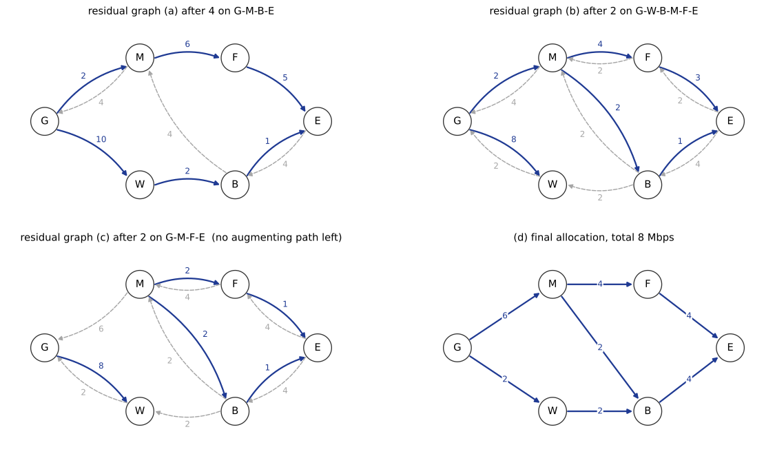
Residual graphs after each augmentation of Ford–Fulkerson on the Princeton network, and the final 8 Mbps allocation. Solid blue arcs are remaining forward capacity, dashed grey arcs are backward (cancellable) flow. In panel (c) the only residual arc out of \(G\) leads to \(W\), from which nothing but \(G\) is reachable, so the algorithm halts and \(\{G,W\}\) is the minimum cut.
Splitting the video across paths is what makes 8 Mbps achievable against the 5 Mbps of the best single path \(G\)–\(M\)–\(F\)–\(E\) — Problem 13.1’s packet-switching argument applied to routing.
Problem 13.4 — Dynamic alternative routing
Dynamic alternative routing. We did not get a chance to talk about routing in circuit-switched networks. A major brand there is Dynamic Alternative Routing DAR, which was adopted by British Telecom in 1996 for their networks.
Suppose that, instead of having fixed paths to route packets from a source to a destination, we want the routes to change dynamically in response to network conditions. We will consider such a protocol, DAR, in the case of a fully-connected graph.
We want the routing to adapt dynamically to the link utilization and select a new path if the current one is too busy. Each possible session (source–destination pair) has an associated backup node. When a session is initiated, it first tries to send its traffic along the direct link. If the direct link fails because it is full, the session tries to use the two-hop path with the backup node. If the backup path fails too because it is busy, the session fails and selects a new backup node from the network. Clearly, the backup node should not be the same node as the destination of the session.
One possible problem with this scheme is that many sessions may end up using two-hop paths. Then we are not being very efficient, since we are using double the capacity compared with a one-hop path. Therefore, DAR reserves a fraction \(t_l\) of each link \(l\) for direct, one-hop sessions (sessions that use the direct link between the source and destination, as opposed to the backup path). We call this parameter, \(t_l \in (0,1)\), the trunk reservation coefficient. Each link \(l\) in the network has an overall capacity of \(c_l\) Mbps and is bidirectional. The non-reserved capacity, \(c_l - t_l c_l\), may be used for either direct or indirect sessions.
(a) Suppose we have the full mesh shown in Figure 13.14, a complete graph \(K_5\) on nodes \(A\), \(B\), \(C\), \(D\), \(E\) (all ten pairs joined). Let \(c_l = 10\) Mbps, \(t_l = 0.1\) for all \(l\). The backup nodes are initialized as in Table 13.1: session \((B,C)\) has backup \(A\), session \((C,B)\) has backup \(A\), session \((A,C)\) has backup \(E\).
The following events occur in sequence: 1. Ten parallel sessions of \((B,C)\) begin. 2. Ten parallel sessions of \((C,B)\) begin. 3. Ten parallel sessions of \((A,C)\) begin. Assume the sessions last a long time and each session consumes 1 Mbps. Fill in Table 13.2, whose rows are the links \((A,B)\), \((A,C)\), \((A,E)\), \((B,C)\), \((C,E)\) and whose two columns are “unreserved capacity used [session]” and “reserved capacity used [session]”. Remember that sessions and links are two different concepts. One row has been filled out for you as an example: link \((B,C)\) has unreserved capacity used 9 Mbps [\(9 \times (B,C)\)] and reserved capacity used 1 [\(1 \times (B,C)\)].
(b) Repeat (a) without the trunk reservation scheme.
(c) What is the efficiency of link utilization, i.e., the number of sessions divided by the total network capacity used, under (a) and (b), respectively? (difficulty: \(\star\star\))
Trunk reservation is the more efficient scheme, \(29/47\) against \(30/50\). Three conventions are forced by the book’s worked row: each link’s \(c_l = 10\) Mbps is one pool shared by both directions (otherwise the \((C,B)\) sessions would go direct and the exercise collapses); the reserved \(t_lc_l = 1\) Mbps serves only sessions whose direct link it is; and a session failing both the direct link and the backup path is lost, the source then re-randomizing its backup node (sticky random routing).
(a) Event 1: the ten \((B,C)\) sessions are direct, so both pools are open and all ten fit, filling link \((B,C)\) at \(9+1 = 10\). Event 2: link \((B,C)\) being full, the \((C,B)\) sessions take \(C\)–\(A\)–\(B\), spending 1 Mbps on each of \((A,C)\) and \((A,B)\), but as indirect traffic only from the 9 Mbps unreserved slices; nine fit and the tenth is lost, the idle reserved Mbps being off-limits to it. Event 3: link \((A,C)\) holds 9 Mbps of that indirect traffic but its reserved Mbps is untouched and \((A,C)\) sessions are direct, so one is carried on the direct link — precisely what trunk reservation exists to produce — and the other nine go \(A\)–\(E\)–\(C\) over the empty \((A,E)\), \((C,E)\).
| Link | Unreserved capacity used [session] | Reserved capacity used [session] |
|---|---|---|
| (A,B) | 9 Mbps [\(9 \times (C,B)\)] | 0 |
| (A,C) | 9 Mbps [\(9 \times (C,B)\)] | 1 Mbps [\(1 \times (A,C)\)] |
| (A,E) | 9 Mbps [\(9 \times (A,C)\)] | 0 |
| (B,C) | 9 Mbps [\(9 \times (B,C)\)] | 1 Mbps [\(1 \times (B,C)\)] |
| (C,E) | 9 Mbps [\(9 \times (A,C)\)] | 0 |
The other five links carry nothing; \(29\) of \(30\) sessions are carried, consuming \(9+10+9+10+9 = 47\) Mbps.
(b) With \(t_l = 0\), event 1 is unchanged, all ten \((C,B)\) sessions now fit on \(C\)–\(A\)–\(B\) since the full 10 Mbps of \((A,C)\) and \((A,B)\) is open to indirect traffic, and link \((A,C)\) is then saturated with no protected slice, so all ten \((A,C)\) sessions are pushed onto \(A\)–\(E\)–\(C\).
| Link | Capacity used [session] |
|---|---|
| (A,B) | 10 Mbps [\(10 \times (C,B)\)] |
| (A,C) | 10 Mbps [\(10 \times (C,B)\)] |
| (A,E) | 10 Mbps [\(10 \times (A,C)\)] |
| (B,C) | 10 Mbps [\(10 \times (B,C)\)] |
| (C,E) | 10 Mbps [\(10 \times (A,C)\)] |
All \(30\) sessions are carried, consuming \(50\) Mbps.
(c) \(\eta_{(a)} = 29/47 \approx 0.6170\) against \(\eta_{(b)} = 30/50 = 0.6000\). Scheme (b) carries one more session yet spends 3 Mbps more doing it: the \((A,C)\) session that (a) routed on one hop now takes two, as does the extra session. Since \(\eta\) is the reciprocal of the mean links per carried session, (a) sits at \(1.62\) links per session against \(1.67\).
import numpy as np
from itertools import combinations

NODES = "ABCDE"
LINKS = [frozenset(e) for e in combinations(NODES, 2)]
C, RATE = 10.0, 1.0                       # Mbps per link, Mbps per session

class Net:
    """Full mesh. Each link holds one shared pool of C Mbps; t*C of it is
    reserved for sessions whose direct link it is."""
    def __init__(self, t):
        self.t = t
        self.res = {l: t * C for l in LINKS}       # reserved slice, direct only
        self.un  = {l: (1 - t) * C for l in LINKS} # free to anyone
        self.log = {l: {'un': [], 'res': []} for l in LINKS}

    def direct(self, s, d):                        # one-hop attempt
        l = frozenset((s, d))
        for pool, tag in ((self.un, 'un'), (self.res, 'res')):
            if pool[l] >= RATE:
                pool[l] -= RATE
                self.log[l][tag].append((s, d))
                return True
        return False

    def indirect(self, s, d, k):                   # two-hop via tandem k
        l1, l2 = frozenset((s, k)), frozenset((k, d))
        if self.un[l1] >= RATE and self.un[l2] >= RATE:
            for l in (l1, l2):
                self.un[l] -= RATE
                self.log[l]['un'].append((s, d))
            return True
        return False

def run(t, backup, events):
    net, carried, lost = Net(t), 0, 0
    for (s, d), n in events:
        for _ in range(n):
            if net.direct(s, d):
                carried += 1
            elif net.indirect(s, d, backup[(s, d)]):
                carried += 1
            else:
                lost += 1
                pool = [k for k in NODES if k not in (s, d, backup[(s, d)])]
                backup[(s, d)] = pool[0]           # re-randomize the tandem
    return net, carried, lost

def tally(pairs):
    out, seen = [], []
    for p in pairs:
        if p not in seen:
            seen.append(p)
            out.append("%d x (%s, %s)" % (pairs.count(p), p[0], p[1]))
    return "; ".join(out) if out else "-"

events = [(('B','C'), 10), (('C','B'), 10), (('A','C'), 10)]
for t, name in ((0.1, "(a) with trunk reservation, t = 0.1"), (0.0, "(b) no trunk reservation")):
    backup = {('B','C'): 'A', ('C','B'): 'A', ('A','C'): 'E'}
    net, carried, lost = run(t, backup, events)
    print(name)
    used = 0.0
    for l in [frozenset(x) for x in ("AB","AC","AE","BC","CE","AD","BD","BE","CD","DE")]:
        u = (1 - t) * C - net.un[l]
        r = t * C - net.res[l]
        if u + r == 0:
            continue
        used += u + r
        print("   (%s) unreserved %.0f Mbps [%s] | reserved %.0f Mbps [%s]"
              % (", ".join(sorted(l)), u, tally(net.log[l]['un']), r, tally(net.log[l]['res'])))
    print("   sessions carried = %d, blocked = %d, capacity used = %.0f Mbps, "
          "efficiency = %.4f" % (carried, lost, used, carried / used))
(a) with trunk reservation, t = 0.1
   (A, B) unreserved 9 Mbps [9 x (C, B)] | reserved 0 Mbps [-]
   (A, C) unreserved 9 Mbps [9 x (C, B)] | reserved 1 Mbps [1 x (A, C)]
   (A, E) unreserved 9 Mbps [9 x (A, C)] | reserved 0 Mbps [-]
   (B, C) unreserved 9 Mbps [9 x (B, C)] | reserved 1 Mbps [1 x (B, C)]
   (C, E) unreserved 9 Mbps [9 x (A, C)] | reserved 0 Mbps [-]
   sessions carried = 29, blocked = 1, capacity used = 47 Mbps, efficiency = 0.6170
(b) no trunk reservation
   (A, B) unreserved 10 Mbps [10 x (C, B)] | reserved 0 Mbps [-]
   (A, C) unreserved 10 Mbps [10 x (C, B)] | reserved 0 Mbps [-]
   (A, E) unreserved 10 Mbps [10 x (A, C)] | reserved 0 Mbps [-]
   (B, C) unreserved 10 Mbps [10 x (B, C)] | reserved 0 Mbps [-]
   (C, E) unreserved 10 Mbps [10 x (A, C)] | reserved 0 Mbps [-]
   sessions carried = 30, blocked = 0, capacity used = 50 Mbps, efficiency = 0.6000
(The simulator reproduces the book’s supplied row for link \((B,C)\), confirming the reading conventions.)
Method (2): the static snapshot understates the effect, since the real failure mode is dynamic — under load, directly-blocked calls spill onto two-hop paths, whose doubled consumption causes further direct failures, and the network can lock into routing almost everything the expensive way. A discrete-event simulation of the same mesh under Poisson arrivals:
import numpy as np, heapq
from itertools import permutations, combinations

NODES, C = "ABCDE", 10
PAIRS = list(permutations(NODES, 2))
EDGES = [frozenset(e) for e in combinations(NODES, 2)]

def sim(t, a, T=4000.0, seed=1):
    """DAR on the 5-node mesh: Poisson arrivals rate a per ordered pair,
    unit-mean holding times, sticky-random tandem, trunk reservation t."""
    rng = np.random.default_rng(seed)
    resv = int(round(t * C))
    occ = {l: 0 for l in EDGES}
    tandem = {p: rng.choice([k for k in NODES if k not in p]) for p in PAIRS}
    ev = [(rng.exponential(1/a), 'arr', p) for p in PAIRS]
    heapq.heapify(ev)
    carried = blocked = live = 0
    circuit_area = session_area = 0.0
    clock = 0.0
    while ev:
        tm, kind, pay = heapq.heappop(ev)
        if tm > T:
            break
        circuit_area += sum(occ.values()) * (tm - clock)
        session_area += live * (tm - clock)
        clock = tm
        if kind == 'arr':
            s, d = pay
            heapq.heappush(ev, (tm + rng.exponential(1/a), 'arr', pay))
            l = frozenset((s, d))
            if occ[l] < C:                                  # direct: whole link
                occ[l] += 1; carried += 1; live += 1
                heapq.heappush(ev, (tm + rng.exponential(1.0), 'dep', (l,)))
            else:
                k = tandem[(s, d)]
                l1, l2 = frozenset((s, k)), frozenset((k, d))
                if occ[l1] <= C - resv - 1 and occ[l2] <= C - resv - 1:
                    occ[l1] += 1; occ[l2] += 1; carried += 1; live += 1
                    heapq.heappush(ev, (tm + rng.exponential(1.0), 'dep', (l1, l2)))
                else:                                        # lost; re-pick tandem
                    blocked += 1
                    tandem[(s, d)] = rng.choice([x for x in NODES if x not in (s, d)])
        else:
            for l in pay:
                occ[l] -= 1
            live -= 1
    return blocked / (carried + blocked), session_area / max(circuit_area, 1e-9)

print(" offered   --- no reservation ---   --- t = 0.1 ---")
print(" a/pair     P(block)   efficiency     P(block)   efficiency")
for a in [2, 4, 6, 8, 10, 12]:
    b0, e0 = sim(0.0, a)
    b1, e1 = sim(0.1, a)
    print("  %5.1f      %6.3f      %6.3f        %6.3f      %6.3f" % (a, b0, e0, b1, e1))
offered   --- no reservation ---   --- t = 0.1 ---
a/pair     P(block)   efficiency     P(block)   efficiency
   2.0       0.000       0.994         0.000       0.994
   4.0       0.122       0.878         0.108       0.937
   6.0       0.363       0.842         0.313       0.944
   8.0       0.505       0.844         0.452       0.959
  10.0       0.594       0.850         0.546       0.972
  12.0       0.655       0.859         0.614       0.980
Without reservation the efficiency collapses to about \(0.84\) once loaded and stays there; with \(t_l = 0.1\) it rises toward 1, the protected slice forcing calls back onto direct links, while blocking is \(4\)–\(5\) points lower at every load. Reserving capacity for direct traffic is Pareto-better here, so the toy ranking is not an artifact.
Problem 13.5 — Spanning tree
Spanning tree. Routing in an inter-connected set of local area networks (LANs) is easier than over the entire Internet. The connections among LANs are called bridges, or switches. Each has multiple ports, with one port connecting to one LAN. A bridge listens to each packet arriving on a port and copies the source address in that packet’s header into the database of hosts reachable from that port. This “learning bridge” protocol works well, except when there are loops in the graph of LANs and bridges, so we need a spanning tree: a cycle-free subgraph connecting all the LANs, so that there is only one way to forward a packet from one device to another. Here we tackle the problem of distributedly discovering a spanning tree (not necessarily the minimum spanning tree), a protocol invented by Perlman in 1985.
Consider the set of LAN segments and bridges depicted in Figure 13.15. The figure has two node types: each LAN segment is a horizontal line with host circles hanging off it, and each bridge is an oval; the links join bridges to LAN segments. There are five LAN segments and four bridges. Label the bridges \(B_1\) (top), \(B_2\) (upper left), \(B_3\) (lower left), \(B_4\) (lower right) and the segments \(L_1\) (top right), \(L_2\) (upper middle), \(L_3\) (left), \(L_4\) (right), \(L_5\) (bottom). The incidences are: \(B_1\) attaches to \(L_1\), \(L_2\), \(L_4\); \(B_2\) attaches to \(L_2\), \(L_3\); \(B_3\) attaches to \(L_3\), \(L_5\); \(B_4\) attaches to \(L_4\), \(L_5\). Clearly there is a cycle: \(L_2\)–\(B_1\)–\(L_4\)–\(B_4\)–\(L_5\)–\(B_3\)–\(L_3\)–\(B_2\)–\(L_2\). One way to arrive at a consistent spanning tree is to have the bridge with the smallest ID number as the root of the tree, and each of the other bridges reach this root bridge through the smallest-hop-count path. That is easy with a global view. But how to do it distributedly, with message passing only between neighbours? How do the nodes even agree on which bridge is the root?
One possibility is to ask each bridge to announce, during each timeslot, a message with three fields: the ID of the bridge believed to be the root; the number of hops to reach that root bridge from this bridge; and the ID of this bridge.
(a) Initially, each bridge only has local information about itself. What are the messages from the four bridges in Figure 13.15?
(b) Upon receiving a message, each bridge selects the root bridge and discovers the way to reach it by applying the following ordered list of criteria. 1. The bridge with a lower ID number wins and becomes the new root bridge (as believed by this bridge). 2. If there are multiple paths to reach the same root bridge, the path with the smallest hop count wins. 3. If there are multiple equal-hop-count paths to reach the same root bridge, the path announced from a bridge with a smaller ID number wins. Each bridge then updates the root bridge field of the message, increases the hop count by 1, and sends the new message to its neighbours, except of course those neighbours that have a shorter path toward the same root bridge. Write down the evolution of the messages for the bridges in Figure 13.15. Does it converge to a spanning tree?
(c) Even after convergence, the root bridge keeps sending the message once every regular period. Why is that? Consider what happens when a bridge fails. (difficulty: \(\star\star\star\))
Rules 1–3 are exactly lexicographic order on the message triple \((\text{root},\text{hops},\text{self})\), so the protocol is the Bellman–Ford iteration (13.1) with the scalar cost replaced by \((\text{root},\text{hops})\), the sender-ID tie-break making the order total and the fixed point unique. Taking \(B_i\) to have ID \(i\), the induced bridge adjacency is the 4-cycle \(B_1 \sim B_2\) (over \(L_2\)), \(B_2 \sim B_3\) (\(L_3\)), \(B_3 \sim B_4\) (\(L_5\)), \(B_4 \sim B_1\) (\(L_4\)); with \(4+5 = 9\) nodes and \(3+2+2+2 = 9\) links, a spanning tree must drop exactly one link.
(a) Each bridge knows only itself, so claims to be the root at 0 hops:
\[ B_1: (1,0,1), \qquad B_2: (2,0,2), \qquad B_3: (3,0,3), \qquad B_4: (4,0,4). \]
(b) Yes, it converges after two rounds. Each bridge takes the lexicographic minimum of its own claim \((\text{self},0)\) and every received \((\text{root},\text{hops}+1)\), the winning port becoming its root port.
- \(t = 1\): \(B_2\) hears \((1,0,1)\) over \(L_2\) and \((3,0,3)\) over \(L_3\), so \(B_2 \to (1,1,2)\), root port \(L_2\); symmetrically \(B_4 \to (1,1,4)\), root port \(L_4\). \(B_3\) hears only \((2,0,2)\), \((4,0,4)\), so \(B_3 \to (2,1,3)\), root port \(L_3\). \(B_1\) is unchanged.
- \(t = 2\): \(B_3\) hears \((1,1,2)\) and \((1,1,4)\), both root 1 at 2 hops, so criterion 3 decides on \(2 < 4\): \(B_3 \to (1,2,3)\), root port \(L_3\).
- \(t = 3\): nothing changes.
| \(t\) | \(B_1\) | \(B_2\) | \(B_3\) | \(B_4\) |
|---|---|---|---|---|
| 0 | \((1,0,1)\) | \((2,0,2)\) | \((3,0,3)\) | \((4,0,4)\) |
| 1 | \((1,0,1)\) | \((1,1,2)\) | \((2,1,3)\) | \((1,1,4)\) |
| 2 | \((1,0,1)\) | \((1,1,2)\) | \((1,2,3)\) | \((1,1,4)\) |
| 3 | \((1,0,1)\) | \((1,1,2)\) | \((1,2,3)\) | \((1,1,4)\) |
Which link is dropped is not visible in the table. Each LAN elects a designated bridge — fewest hops to the root, ties by lower ID — and a port forwards iff it is its bridge’s root port or its bridge is designated there, which is the book’s “except those neighbours that have a shorter path toward the same root bridge”:
- \(L_1\): only \(B_1\) (0 hops). Designated \(B_1\).
- \(L_2\): \(B_1\) (0) and \(B_2\) (1). Designated \(B_1\); \(L_2\) is \(B_2\)’s root port, so both ends forward.
- \(L_3\): \(B_2\) (1) and \(B_3\) (2). Designated \(B_2\); \(L_3\) is \(B_3\)’s root port, so both ends forward.
- \(L_4\): \(B_1\) (0) and \(B_4\) (1). Designated \(B_1\); \(L_4\) is \(B_4\)’s root port, so both ends forward.
- \(L_5\): \(B_3\) (2) and \(B_4\) (1). Designated \(B_4\). \(B_3\)’s port onto \(L_5\) is neither its root port (that is \(L_3\)) nor designated, so \(B_3\) blocks it.
Eight links over nine nodes: a tree rooted at \(B_1\) with \(L_1, L_2, L_4\) directly off the root, \(L_3\) below via \(B_2\) and \(L_5\) below via \(B_4\). Every LAN remains reachable; \(B_3\) reaches \(L_5\) the long way through \(L_3, B_2, L_2, B_1, L_4, B_4\).
import matplotlib.pyplot as plt
from matplotlib.patches import Ellipse

PORTS = {1: ['L1', 'L2', 'L4'], 2: ['L2', 'L3'], 3: ['L3', 'L5'], 4: ['L4', 'L5']}
LANS = sorted({l for p in PORTS.values() for l in p})

msg = {b: (b, 0, b) for b in PORTS}          # (believed root, hops to root, own ID)
rootport = {b: None for b in PORTS}
print("t=0:  " + "   ".join("B%d (%d,%d,%d)" % (b, *msg[b]) for b in sorted(PORTS)))

for t in range(1, 5):
    heard = {l: [] for l in LANS}
    for b, m in msg.items():                 # every bridge shouts on every port
        for l in PORTS[b]:
            heard[l].append(m)
    new, newport = {}, {}
    for b in PORTS:
        cands = [(r, h + 1, s, l) for l in PORTS[b] for (r, h, s) in heard[l] if s != b]
        best = min(cands, key=lambda c: c[:3]) if cands else None
        if best and (best[0], best[1]) < (b, 0):        # someone offers a better root
            new[b], newport[b] = (best[0], best[1], b), best[3]
        else:                                            # I am still the root
            new[b], newport[b] = (b, 0, b), None
    changed = (new != msg)
    msg, rootport = new, newport
    print("t=%d:  " % t + "   ".join("B%d (%d,%d,%d)" % (b, *msg[b]) for b in sorted(PORTS))
          + "  | root ports " + ", ".join("B%d:%s" % (b, rootport[b] or 'root')
                                          for b in sorted(PORTS))
          + ("" if changed else "   <- no change, converged"))
    if not changed:
        break

cost = {b: msg[b][1] for b in PORTS}
tree, blocked = [], []
for l in LANS:
    att = [b for b in PORTS if l in PORTS[b]]
    des = min(att, key=lambda b: (cost[b], b))
    for b in att:
        (tree if (b == des or rootport[b] == l) else blocked).append((b, l))
    print("LAN %s: attached %s, hop counts %s -> designated bridge B%d"
          % (l, ["B%d" % b for b in att], [cost[b] for b in att], des))
print("forwarding links:", ["B%d-%s" % e for e in tree])
print("BLOCKED links   :", ["B%d-%s" % e for e in blocked])
print("nodes = %d, links kept = %d  (a tree needs %d)"
      % (len(PORTS) + len(LANS), len(tree), len(PORTS) + len(LANS) - 1))

LP = {'L1': (3.6, 3.1), 'L2': (1.7, 2.1), 'L3': (0.1, 0.7),
      'L4': (3.5, 0.7), 'L5': (1.9, -0.9)}
BP = {1: (2.7, 2.7), 2: (0.5, 1.6), 3: (0.9, -0.1), 4: (3.0, -0.1)}
fig, ax = plt.subplots(figsize=(7.6, 6.0))
for b, l in [(b, l) for b in PORTS for l in PORTS[b]]:
    (x0, y0), (x1, y1) = BP[b], LP[l]
    bad = (b, l) in blocked
    ax.plot([x0, x1], [y0, y1], color='#c0392b' if bad else '0.35',
            lw=2.4 if bad else 1.6, ls='--' if bad else '-', zorder=1)
    if bad:
        ax.text((x0+x1)/2 - .55, (y0+y1)/2 - .1, 'blocked', color='#c0392b', fontsize=10)
for l, (x, y) in LP.items():
    ax.plot([x-.62, x+.62], [y, y], color='0.15', lw=2.4, zorder=2)
    for dx in (-.36, 0, .36):
        ax.plot([x+dx, x+dx], [y, y-.22], color='0.15', lw=1.0, zorder=2)
        ax.add_patch(plt.Circle((x+dx, y-.30), .075, fc='white', ec='0.15', zorder=3))
    ax.text(x+.72, y+.06, l, fontsize=11, color='0.15')
for b, (x, y) in BP.items():
    ax.add_patch(Ellipse((x, y), .95, .46, fc='white', ec='0.15', lw=1.6, zorder=4))
    ax.text(x, y, 'B%d' % b, ha='center', va='center', fontsize=11, zorder=5)
ax.set_title('Figure 13.15 relabelled: bridge B1 wins the root election;\n'
             'B3 blocks its port onto L5, leaving a spanning tree', fontsize=11)
ax.set_xlim(-1.0, 4.8); ax.set_ylim(-1.6, 3.7); ax.axis('off'); ax.set_aspect('equal')
plt.tight_layout()
plt.savefig('nl-ch13-spanning-tree.svg', dpi=150, bbox_inches='tight')
t=0:  B1 (1,0,1)   B2 (2,0,2)   B3 (3,0,3)   B4 (4,0,4)
t=1:  B1 (1,0,1)   B2 (1,1,2)   B3 (2,1,3)   B4 (1,1,4)  | root ports B1:root, B2:L2, B3:L3, B4:L4
t=2:  B1 (1,0,1)   B2 (1,1,2)   B3 (1,2,3)   B4 (1,1,4)  | root ports B1:root, B2:L2, B3:L3, B4:L4
t=3:  B1 (1,0,1)   B2 (1,1,2)   B3 (1,2,3)   B4 (1,1,4)  | root ports B1:root, B2:L2, B3:L3, B4:L4   <- no change, converged
LAN L1: attached ['B1'], hop counts [0] -> designated bridge B1
LAN L2: attached ['B1', 'B2'], hop counts [0, 1] -> designated bridge B1
LAN L3: attached ['B2', 'B3'], hop counts [1, 2] -> designated bridge B2
LAN L4: attached ['B1', 'B4'], hop counts [0, 1] -> designated bridge B1
LAN L5: attached ['B3', 'B4'], hop counts [2, 1] -> designated bridge B4
forwarding links: ['B1-L1', 'B1-L2', 'B2-L2', 'B2-L3', 'B3-L3', 'B1-L4', 'B4-L4', 'B4-L5']
BLOCKED links   : ['B3-L5']
nodes = 9, links kept = 8  (a tree needs 8)
The bridged LAN of Figure 13.15 after convergence. Ovals are bridges, horizontal bars with circles are LAN segments with their hosts. \(B_1\) has the lowest ID and becomes the root; \(B_3\) is two hops away via \(L_3\) and loses the designated-bridge contest on \(L_5\) to \(B_4\), so it blocks that port (dashed red), breaking the single cycle and leaving a spanning tree of eight links over nine nodes.
(c) Because the absence of a message is the only way a bridge can learn that something has died. After convergence every bridge still believes root \(= 1\) and holds a root port whose path may no longer exist; nothing in its own state distinguishes “the root is fine and quiet” from “the root is gone”. So the root re-announces \((1,0,1)\) every hello interval, bridges relay it, and each ages out its stored best message after a max-age timeout. If \(B_1\) fails, \(B_2\) and \(B_4\) stop hearing root 1, age out, reclaim rootship, and the election settles on \(B_2\); the surviving adjacency is the path \(B_2 - B_3 - B_4\), giving hops \(0, 1, 2\), so on \(L_5\) the designated bridge becomes \(B_3\) and \(B_3\)’s blocked port unblocks — necessarily, since \(L_4\) and \(L_5\) now reach the network only through \(B_3\). \(L_1\), hanging off \(B_1\) alone, is genuinely isolated.
The timers are asymmetric: good news travels on arrival, so a returning root is adopted in one round, while bad news travels only by timeout, which is why 802.1D takes 30–50 seconds to heal. The stakes are higher than at layer 3, since an Ethernet frame carries no TTL and a surviving cycle causes a broadcast storm.
Why doesn’t the Internet collapse under congestion?
Problem 14.1 — A numerical example of NUM
A numerical example of NUM. Suppose we have a network whose topology is shown in Figure 14.12.
Figure 14.12 shows four nodes \(B\), \(C\), \(A\), \(D\) and four links. \(B\) and \(C\) sit at the top and are joined by link 2. Link 1 joins \(B\) down to \(A\), which sits in the middle, and link 3 joins \(C\) down to \(A\); so \(B\), \(C\), \(A\) form a triangle with links 2, 1, 3. Link 4 runs from \(A\) down to \(D\) at the bottom. Two end-to-end sessions are drawn as arcs over this topology. Session 1 is an arc from \(B\) down to \(D\), passing to the left of \(A\) (i.e. it is routed \(B \to A \to D\), over links 1 and 4). Session 2 is an arc from \(D\) up to \(A\), drawn to the right of link 4 (i.e. it is routed \(D \to A\), over link 4 alone). Links 2 and 3 carry no session.
(a) Write down the routing matrix \(A\).
(b) Run a numerical example for ten time steps to solve the NUM problem using the link-price and source-rate updates in (14.4) and (14.5). The utility function is a logarithmic function of the source rate. Initialize the link prices to 1, and run the source-rate update step first. Set the step size \(\beta = 1\). Plot the source rates and link prices over time. What are the equilibrium values?
(c) Change the step size \(\beta\) and observe the impact on the convergence of the algorithm. (difficulty: \(\star\star\))
The equilibrium is \(x_1^\star = x_2^\star = 0.5\) Mbps with \(p_4^\star = 2\) and all other prices \(0\). (The printed equation numbers point at the NUM formulation (14.4) and Lagrangian (14.5); the intended iterations are the source update (14.2) and link-price update (14.3). Capacities are not printed, so take \(c_l = 1\) Mbps throughout as in Section 14.3.)
(a) With rows indexing links and columns sessions, \(A_{li} = 1\) iff session \(i\) traverses link \(l\); session 1 uses \(\{1,4\}\) and session 2 uses \(\{4\}\), so
\begin{equation*} A = \begin{bmatrix} 1 & 0 \\ 0 & 0 \\ 0 & 0 \\ 1 & 1 \end{bmatrix}, \qquad A\mathbf{x} = \begin{bmatrix} x_1 \\ 0 \\ 0 \\ x_1 + x_2 \end{bmatrix} \le \begin{bmatrix} 1 \\ 1 \\ 1 \\ 1 \end{bmatrix}. \end{equation*}
Equivalently \(S(1) = \{1\}\), \(S(2) = S(3) = \varnothing\), \(S(4) = \{1,2\}\), and \(L(1) = \{1,4\}\), \(L(2) = \{4\}\).
(b) NUM (14.1) with \(U_i = \log x_i\) is to maximize \(\log x_1 + \log x_2\) subject to \(x_1 \le 1\), \(x_1 + x_2 \le 1\). Link 4 is the only binding constraint, and maximizing on \(x_1 + x_2 = 1\) gives \(x_1^\star = x_2^\star = 0.5\); links 1–3 are then slack, so complementary slackness (Section 14.4.1) forces \(p_1^\star = p_2^\star = p_3^\star = 0\), and the source rule \(x_1 = 1/p_4 = 0.5\) pins \(p_4^\star = 2\). The distributed algorithm, with prices at 1 and the source step first, is
\begin{equation*} q_i[t] = \sum_{l \in L(i)} p_l[t-1], \qquad x_i[t] = \frac{1}{q_i[t]}, \qquad p_l[t] = \left\{ p_l[t-1] + \beta\left(y_l[t] - c_l\right) \right\}^+ . \end{equation*}
By hand at \(t = 1\): \(q_1 = 2\) and \(q_2 = 1\) give \(x = (0.5, 1)\), loads \(y_1 = 0.5\), \(y_4 = 1.5\), hence \(p_1 = 0.5\), \(p_4 = 1.5\).
import numpy as np

A = np.array([[1, 0],
              [0, 0],
              [0, 0],
              [1, 1]], dtype=float)
c = np.ones(4)

def num_iterate(beta, T=10):
    p = np.ones(4)
    X, P = [], []
    for t in range(T):
        q = A.T @ p                                    # path price per session
        x = np.where(q > 0, 1.0 / np.maximum(q, 1e-12), 1e6)
        y = A @ x                                      # load per link
        p = np.maximum(p + beta * (y - c), 0.0)
        X.append(x.copy()); P.append(p.copy())
    return np.array(X), np.array(P)

X, P = num_iterate(1.0, 10)
for t in range(10):
    print("t=%2d  x=%s   p=%s" % (t + 1, np.round(X[t], 4), np.round(P[t], 4)))
t= 1  x=[0.5 1. ]   p=[0.5 0.  0.  1.5]
t= 2  x=[0.5    0.6667]   p=[0.     0.     0.     1.6667]
t= 3  x=[0.6 0.6]   p=[0.     0.     0.     1.8667]
t= 4  x=[0.5357 0.5357]   p=[0.     0.     0.     1.9381]
t= 5  x=[0.516 0.516]   p=[0.   0.   0.   1.97]
t= 6  x=[0.5076 0.5076]   p=[0.     0.     0.     1.9852]
t= 7  x=[0.5037 0.5037]   p=[0.     0.     0.     1.9927]
t= 8  x=[0.5018 0.5018]   p=[0.     0.     0.     1.9964]
t= 9  x=[0.5009 0.5009]   p=[0.     0.     0.     1.9982]
t=10  x=[0.5005 0.5005]   p=[0.     0.     0.     1.9991]
The hand step matches, and after ten iterations the iterates sit within \(5\times10^{-4}\) of the analytic \(x^\star = (0.5,0.5)\), \(p^\star = (0,0,0,2)\). Link 1’s price falls to zero after two steps and stays there: it is not a bottleneck, so it charges nothing.
import matplotlib.pyplot as plt

t = np.arange(1, 11)
fig, ax = plt.subplots(1, 2, figsize=(10, 3.6))
ax[0].plot(t, X[:, 0], 'o-', label='session 1')
ax[0].plot(t, X[:, 1], 's--', label='session 2')
ax[0].axhline(0.5, color='gray', lw=0.8, ls=':')
ax[0].set_xlabel('iteration t'); ax[0].set_ylabel('source rate')
ax[0].set_title('source rates, beta = 1'); ax[0].legend()
for l in range(4):
    ax[1].plot(t, P[:, l], marker='o', ms=3, label='link %d' % (l + 1))
ax[1].axhline(2.0, color='gray', lw=0.8, ls=':')
ax[1].set_xlabel('iteration t'); ax[1].set_ylabel('link price')
ax[1].set_title('link prices, beta = 1'); ax[1].legend()
plt.tight_layout()
plt.savefig('nl-ch14-num-convergence.svg', dpi=150, bbox_inches='tight')
plt.show()
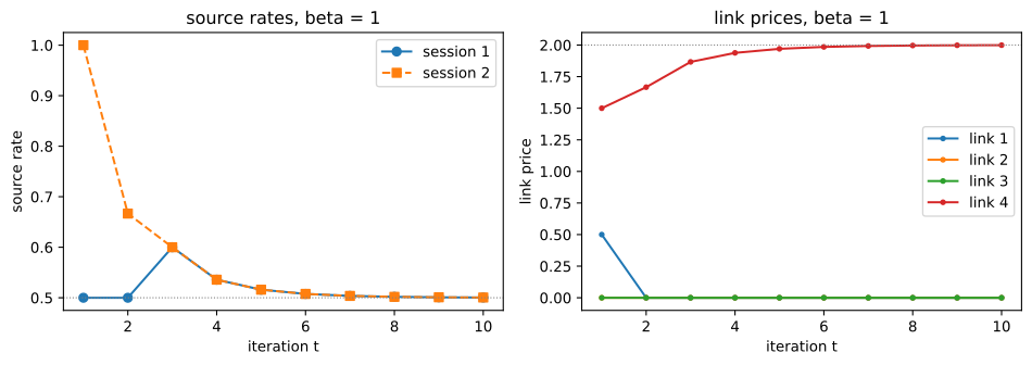
Source rates (left) and link prices (right) over ten iterations of the NUM algorithm with \(\beta = 1\). Both sessions settle at 0.5 Mbps; only the bottleneck link 4 keeps a positive price, converging to 2.
(c) \(\beta\) is the gradient step for the dual price problem (Figure 14.11): small \(\beta\) is safe but slow, large \(\beta\) overshoots.
fig, ax = plt.subplots(figsize=(7, 4))
for beta in [0.1, 0.5, 1.0, 2.0, 3.0]:
    Xb, Pb = num_iterate(beta, 40)
    ax.plot(np.arange(1, 41), Xb[:, 0], label='beta = %.1f' % beta)
ax.axhline(0.5, color='gray', lw=0.8, ls=':')
ax.set_xlabel('iteration t'); ax.set_ylabel('session-1 rate')
ax.set_title('effect of the stepsize on convergence')
ax.legend()
plt.tight_layout()
plt.savefig('nl-ch14-stepsize.svg', dpi=150, bbox_inches='tight')
plt.show()

for beta in [0.1, 0.5, 1.0, 2.0, 3.0, 4.0, 5.0, 6.0, 8.0]:
    Xb, Pb = num_iterate(beta, 400)
    tail = Xb[-50:, 0]
    print("beta=%4.1f  x1[400]=%.4f  tail range [%.4f, %.4f]"
          % (beta, Xb[-1, 0], tail.min(), tail.max()))
beta= 0.1  x1[400]=0.5000  tail range [0.5000, 0.5000]
beta= 0.5  x1[400]=0.5000  tail range [0.5000, 0.5000]
beta= 1.0  x1[400]=0.5000  tail range [0.5000, 0.5000]
beta= 2.0  x1[400]=0.5000  tail range [0.5000, 0.5000]
beta= 3.0  x1[400]=0.5000  tail range [0.5000, 0.5000]
beta= 4.0  x1[400]=0.4876  tail range [0.4868, 0.5132]
beta= 5.0  x1[400]=0.2731  tail range [0.2729, 0.7293]
beta= 6.0  x1[400]=0.7204  tail range [0.1223, 1.0689]
beta= 8.0  x1[400]=0.0000  tail range [0.0000, 0.0000]
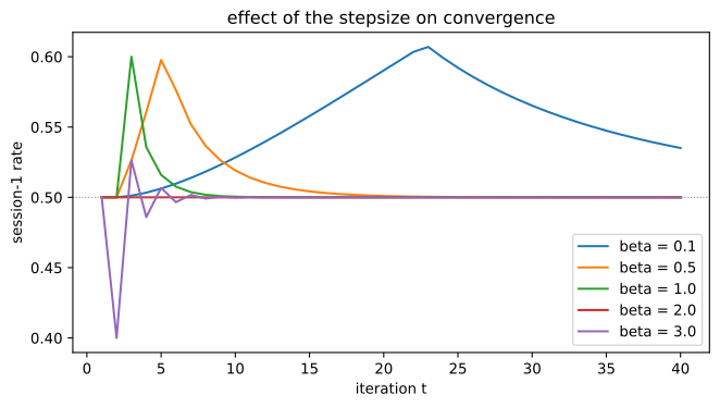
Session-1 rate over 40 iterations for five step sizes. \(\beta = 0.1\) drifts up to 0.607 by step 23 and is still at 0.535 at step 40; \(\beta = 1\) and \(\beta = 2\) land on 0.5 within a few steps; \(\beta = 3\) rings down to it in a damped oscillation.
Three regimes: (i) \(\beta = 0.1\) still sits at \(0.535\) after 40 iterations, converging only by step 400; (ii) \(0.5 \le \beta \le 3\) converges in a handful of steps, monotonically or with quick ringing; (iii) \(\beta \ge 4\) fails to settle — a two-cycle at \(\beta = 4\), swings of \(0.27\)–\(0.73\) at \(\beta = 5\), and at \(\beta = 8\) prices blow past \(10^4\) while rates collapse to zero.
The threshold is exact. Near equilibrium the price map is \(p_4 \mapsto p_4 + \beta(2/p_4 - 1)\), with derivative \(1 - 2\beta/(p_4^\star)^2 = 1 - \beta/2\) at \(p_4^\star = 2\), so the fixed point is locally stable iff \(|1 - \beta/2| < 1\), i.e. \(0 < \beta < 4\), and \(\beta = 2\) zeroes the derivative, which is why it is fastest. The safe range depends on the equilibrium price, hence on capacities and session counts that no single link knows.
Problem 14.2 — TCP slow start
TCP slow start. We learned the primary mode of operation of TCP Reno, where the congestion window size, denoted as \(w\) in the homework problems, increases by 1 for each RTT. Equivalently, \(w\) increases by \(\frac{1}{w}\) for each ACK received. This operational mode is called congestion avoidance.
However, this results in a linear increase of \(w\) over time. At the beginning of a TCP connection, we would like to quickly ramp up \(w\) before transitioning to congestion avoidance mode. Most TCP protocols have a (somewhat confusingly named) slow start phase that accomplishes this. In this mode, \(w\) increases by 1 for each ACK received.
(a) If we plot \(w\) versus time, instead of having a linear increase as in congestion avoidance, what kind of increase do we see in slow start?
(b) Assume \(w\) starts at 1. Draw a space-time diagram for the slow start phase over four RTTs. (difficulty: \(\star\))
(a) Exponential: the window doubles every RTT. A sender with window \(w\) puts \(w\) packets in flight and collects \(w\) ACKs one RTT later, so congestion avoidance adds \(w\cdot\tfrac1w = 1\) per RTT, giving \(w[t] = w[0] + t\), while slow start adds \(w \cdot 1 = w\), giving
\begin{equation*} w[t+1] = 2w[t], \qquad w[t] = w[0]\,2^{t} = 2^{t} \ \text{ for } w[0] = 1 . \end{equation*}
In continuous time the two modes are \(\dot w = 1/\text{RTT}\) against \(\dot w = w/\text{RTT}\); on a \(\log_2\) axis slow start is a line of slope 1 per RTT.
import numpy as np
import matplotlib.pyplot as plt

t = np.arange(0, 9)
ss = 2.0 ** t          # slow start
ca = 1.0 + t           # congestion avoidance

fig, ax = plt.subplots(1, 2, figsize=(9, 3.4))
ax[0].step(t, ss, where='post', label='slow start  w=2^t')
ax[0].step(t, ca, where='post', label='congestion avoidance  w=1+t')
ax[0].set_xlabel('time (RTTs)'); ax[0].set_ylabel('w')
ax[0].legend(); ax[0].set_title('linear scale')
ax[1].step(t, ss, where='post', label='slow start')
ax[1].step(t, ca, where='post', label='congestion avoidance')
ax[1].set_yscale('log', base=2)
ax[1].set_xlabel('time (RTTs)'); ax[1].set_ylabel('w (log2 scale)')
ax[1].legend(); ax[1].set_title('log scale: slow start is a straight line')
plt.tight_layout()
plt.savefig('nl-ch14-slow-start-growth.svg', dpi=150, bbox_inches='tight')
plt.show()

print("w after t RTTs, slow start:", ss[:6].astype(int))
print("w after t RTTs, cong. avoid.:", ca[:6].astype(int))
w after t RTTs, slow start: [ 1  2  4  8 16 32]
w after t RTTs, cong. avoid.: [1 2 3 4 5 6]
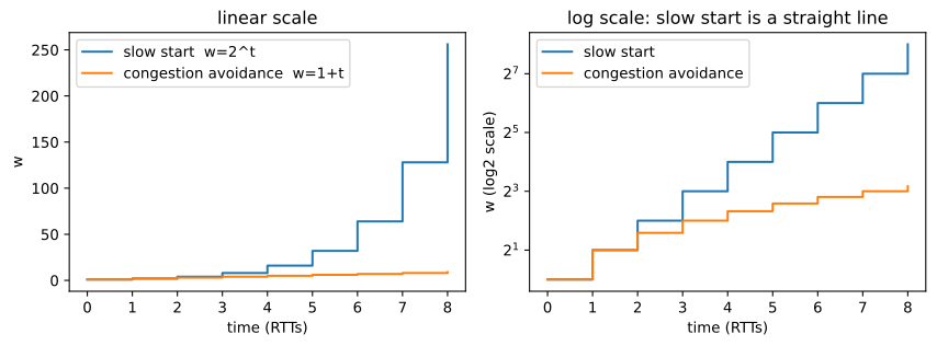
Window growth in the two modes. Slow start doubles each RTT (1, 2, 4, 8, 16, 32); congestion avoidance adds 1 each RTT.
“Slow start” is the more aggressive mode, slow only against the pre-1988 practice of dumping a full advertised window on the first RTT; it ends at ssthresh or at the first loss, when the sender switches to congestion avoidance.
(b) In the convention of Figure 14.3 — vertical sender and receiver lines, time downward, solid diagonals data and dashed diagonals ACKs — the sender transmits 1, 2, 4, 8 packets over the four RTTs, reaching \(w = 16\) with 15 packets sent.
fig, ax = plt.subplots(figsize=(6.5, 7))
ax.axvline(0.0, color='k', lw=1.2)
ax.axvline(1.0, color='k', lw=1.2)
ax.text(0.0, -0.18, 'Sender', ha='center', fontsize=11)
ax.text(1.0, -0.18, 'Receiver', ha='center', fontsize=11)

for k in range(4):
    n = 2 ** k                      # window in force during RTT k+1
    for j in range(n):
        ts = k + (j / n) * 0.34     # packets of one window, slightly staggered
        ax.annotate('', xy=(1.0, ts + 0.5), xytext=(0.0, ts),
                    arrowprops=dict(arrowstyle='->', color='C0', lw=1.0))
        ax.annotate('', xy=(0.0, ts + 1.0), xytext=(1.0, ts + 0.5),
                    arrowprops=dict(arrowstyle='->', color='C3', lw=1.0, ls='--'))
    ax.text(-0.06, k + 0.02, 'w=%d' % n, ha='right', va='top', fontsize=11)
    ax.text(-0.30, k + 0.5, 'RTT %d' % (k + 1), ha='left', va='center',
            fontsize=10, color='gray')
ax.text(-0.06, 4.02, 'w=16', ha='right', va='top', fontsize=11)

ax.set_xlim(-0.42, 1.25); ax.set_ylim(4.5, -0.35)
ax.set_xticks([]); ax.set_yticks([0, 1, 2, 3, 4])
ax.set_ylabel('time (RTTs)')
ax.set_title('TCP slow start: 1, 2, 4, 8 packets over four RTTs')
for s in ['top', 'right', 'bottom']:
    ax.spines[s].set_visible(False)
plt.tight_layout()
plt.savefig('nl-ch14-slow-start.svg', dpi=150, bbox_inches='tight')
plt.show()

w = 1
for k in range(1, 6):
    print("start of RTT %d: w = %2d   (packets sent this RTT = %2d)" % (k, w, w))
    w = 2 * w
print("total packets sent in the first four RTTs =", 1 + 2 + 4 + 8)
start of RTT 1: w =  1   (packets sent this RTT =  1)
start of RTT 2: w =  2   (packets sent this RTT =  2)
start of RTT 3: w =  4   (packets sent this RTT =  4)
start of RTT 4: w =  8   (packets sent this RTT =  8)
start of RTT 5: w = 16   (packets sent this RTT = 16)
total packets sent in the first four RTTs = 15
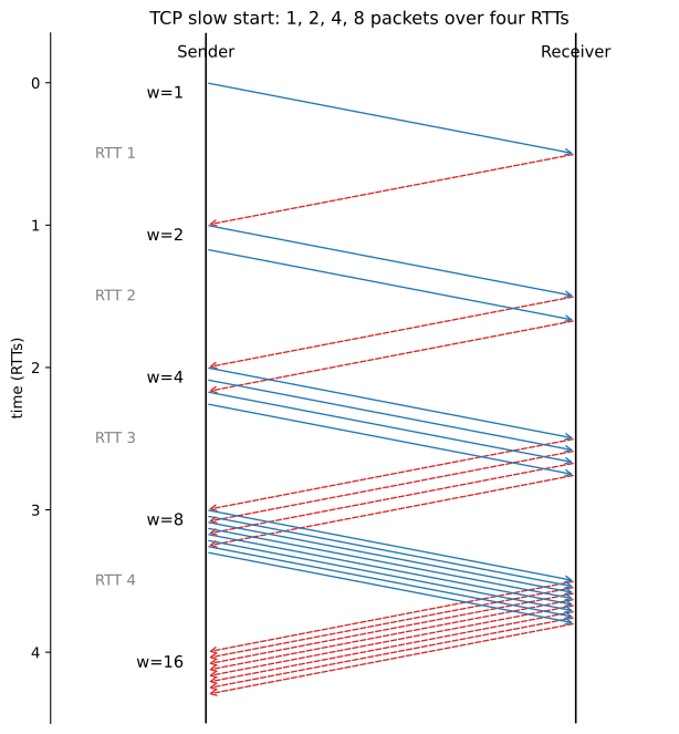
Space-time diagram of slow start over four RTTs. Solid arrows are data packets, dashed arrows are ACKs. Each ACK both slides the window by one and grows it by one, so every arriving ACK releases two packets and the window doubles per RTT.
The picture shows the mechanism: each ACK both slides the window by one and grows it by one, so two packets leave for every one that is acknowledged, which is the doubling.
Problem 14.3 — TCP Reno congestion window
TCP Reno congestion window. Recall that the congestion window length changes with time as follows during TCP Reno’s congestion avoidance phase.
- If an ACK is received, then increase \(w\) by \(\frac{1}{w}\).
- If congestion is detected, then decrease \(w\) by \(\frac{w}{2}\).
Suppose the probability of failed transmission is \(p\); the probability of a successful transmission is then \(1-p\). The transmission rate \(x = \frac{w}{RTT}\) packets per second.
(a) Write down the equation for the expected change of \(w\) per time step.
(b) At equilibrium, the expected change is 0. Using (a), show that \(x_r = \frac{1}{RTT}\sqrt{\frac{2(1-p)}{p}}\). (difficulty: \(\star\star\))
(a) One time step is one transmission opportunity, giving the window \(1/w\) with probability \(1-p\) and \(-w/2\) with probability \(p\):
\begin{equation*} \mathbb{E}\big[\Delta w[t]\big] \;=\; (1-p)\cdot \frac{1}{w[t]} \;+\; p \cdot \left(-\frac{w[t]}{2}\right) \;=\; \frac{1-p}{w[t]} \;-\; \frac{p\, w[t]}{2}. \end{equation*}
This is the per-packet form of equation (14.6), whose per-second version \(\mathbb{E}[\dot w] = x(1-q)/w - xqw/2\) differs only by the common factor \(x\), which cannot move the zero.
(b) Setting the drift to zero at \(w_r > 0\) with \(0 < p < 1\),
\begin{equation*} \frac{1-p}{w_r} = \frac{p\, w_r}{2} \quad\Longrightarrow\quad 2(1-p) = p\, w_r^2 \quad\Longrightarrow\quad w_r^2 = \frac{2(1-p)}{p} \quad\Longrightarrow\quad w_r = \sqrt{\frac{2(1-p)}{p}}, \end{equation*}
taking the positive root, and \(x = w/RTT\) gives
\begin{equation*} \boxed{\;x_r = \frac{w_r}{RTT} = \frac{1}{RTT}\sqrt{\frac{2(1-p)}{p}}\;} \end{equation*}
as required. It is the unique stable zero, since \(g(w) = (1-p)/w - pw/2\) is strictly decreasing on \(w > 0\), so the window is pushed back toward \(w_r\) from either side. This is the \(1/\sqrt{p}\) law: throughput falls only as \(\sqrt{p}\) but linearly in \(RTT\), so a long-haul session is structurally penalized at the same bottleneck and loss rate, and a high rate demands an absurd loss rate — 1 Gbps at \(RTT = 100\) ms with 1500-byte packets needs \(w_r \approx 8333\), hence \(p \approx 3\times10^{-8}\).
Checking the algebra and the stability claim:
import numpy as np
rng = np.random.default_rng(0)

def wstar(p):
    return np.sqrt(2.0 * (1.0 - p) / p)

def simulate(p, T, w0=1.0):
    w, s = w0, 0.0
    for t in range(T):
        if rng.random() < p:
            w = max(w - w / 2.0, 1.0)     # multiplicative decrease
        else:
            w = w + 1.0 / w               # additive increase, 1/w per ACK
        s += w
    return s / T

print(" p      w* = sqrt(2(1-p)/p)   drift at w*      MC mean w")
for p in [0.2, 0.1, 0.05, 0.01]:
    ws = wstar(p)
    drift = (1 - p) / ws - p * ws / 2
    print("%5.2f   %14.4f   %12.2e   %10.4f" % (p, ws, drift, simulate(p, 400_000)))
p      w* = sqrt(2(1-p)/p)   drift at w*      MC mean w
0.20           2.8284      -5.55e-17       3.1717
0.10           4.2426       2.78e-17       4.6643
0.05           6.1644       0.00e+00       6.6749
0.01          14.0712       0.00e+00      15.2676
The drift vanishes at \(w_r\) to machine precision. The simulated long-run mean window sits \(8\)–\(12\%\) above \(w_r\), and that gap is real rather than noise: \(g\) is convex, so \(\mathbb{E}[g(w)] = 0\) under the invariant law places \(\mathbb{E}[w]\) above the root by Jensen. The boxed formula is the zero-drift point the problem asks for, a mild underestimate of mean throughput.
Problem 14.4 — TCP Vegas
TCP Vegas. TCP Vegas tries to anticipate congestion by estimating delay. In this scheme, the congestion window size is changed on the basis of the timings of the ACKs it has received. Specifically, we have
\begin{equation*} w[t+1] = \begin{cases} w[t] + 1 & \text{if } \dfrac{w[t]}{d} - \dfrac{w[t]}{D[t]} < \beta \\[2mm] w[t] - 1 & \text{if } \dfrac{w[t]}{d} - \dfrac{w[t]}{D[t]} > \beta \\[2mm] w[t] & \text{otherwise,} \end{cases} \end{equation*}
where \(d\) is the minimum RTT observed historically, \(D[t]\) is the RTT observed at time \(t\), and \(\beta\) is a threshold. So, \(\frac{w}{d}\) is the expected rate and \(\frac{w}{D}\) is the observed rate, and \(w\) decreases (increases) if the expected rate is greater (smaller) than the actual rate by \(\beta\).
Suppose
\begin{equation*} D[t] = \begin{cases} t & \text{if } t \le 4 \\ 4 & \text{otherwise,} \end{cases} \end{equation*}
and \(w[1] = 4\), \(\beta = 3\) and \(d = 1\). Plot the evolution of \(w\) versus time for ten time steps. (difficulty: \(\star\star\))
\(w[1..10] = (4, 5, 6, 5, 4, 4, 4, 4, 4, 4)\). With \(d = 1\) the decision statistic is
\begin{equation*} \frac{w[t]}{d} - \frac{w[t]}{D[t]} \;=\; w[t]\left(1 - \frac{1}{D[t]}\right), \end{equation*}
the number of this session’s packets sitting in queues, compared against \(\beta = 3\):
- \(t=1\): \(4(1-1) = 0 < 3\), increase to 5 (no queueing at all).
- \(t=2\): \(5(1-\tfrac12) = 2.5 < 3\), increase to 6.
- \(t=3\): \(6(1-\tfrac13) = 4 > 3\), decrease to 5.
- \(t=4\): \(5(1-\tfrac14) = 3.75 > 3\), decrease to 4.
- \(t \ge 5\): \(D\) is fixed at 4 and \(4\cdot\tfrac34 = 3 = \beta\) exactly, so the window holds forever.
import numpy as np
import matplotlib.pyplot as plt

d, beta = 1.0, 3.0
D = lambda t: float(t) if t <= 4 else 4.0

w = {1: 4.0}
print(" t   D[t]   w[t]   w/d - w/D    vs beta=3   action")
for t in range(1, 11):
    diff = w[t] / d - w[t] / D(t)
    if diff < beta:
        w[t + 1], act, rel = w[t] + 1, "increase", "<"
    elif diff > beta:
        w[t + 1], act, rel = w[t] - 1, "decrease", ">"
    else:
        w[t + 1], act, rel = w[t], "hold", "="
    print("%2d  %5.1f  %5.1f   %8.2f       %s          %s" % (t, D(t), w[t], diff, rel, act))
print()
print("w[1..11] =", [w[t] for t in range(1, 12)])
 t   D[t]   w[t]   w/d - w/D    vs beta=3   action
 1    1.0    4.0       0.00       <          increase
 2    2.0    5.0       2.50       <          increase
 3    3.0    6.0       4.00       >          decrease
 4    4.0    5.0       3.75       >          decrease
 5    4.0    4.0       3.00       =          hold
 6    4.0    4.0       3.00       =          hold
 7    4.0    4.0       3.00       =          hold
 8    4.0    4.0       3.00       =          hold
 9    4.0    4.0       3.00       =          hold
10    4.0    4.0       3.00       =          hold

w[1..11] = [4.0, 5.0, 6.0, 5.0, 4.0, 4.0, 4.0, 4.0, 4.0, 4.0, 4.0]
ts = np.arange(1, 11)
ws = np.array([w[t] for t in ts])

fig, ax = plt.subplots(figsize=(7, 3.8))
ax.step(ts, ws, where='post', marker='o', color='C0', label='w[t]')
ax.plot(ts, [D(t) for t in ts], 's--', color='C3', ms=4, label='D[t] (observed RTT)')
ax.axhline(4, color='gray', lw=0.8, ls=':')
ax.set_xlabel('time step t'); ax.set_ylabel('value')
ax.set_xticks(ts); ax.set_ylim(0, 7)
ax.set_title('TCP Vegas window, d=1, beta=3, w[1]=4')
ax.legend()
plt.tight_layout()
plt.savefig('nl-ch14-vegas-window.svg', dpi=150, bbox_inches='tight')
plt.show()
![TCP Vegas window over ten steps with \(d=1\), \(\beta=3\), \(w[1]=4\). The window rises to 6 while the measured RTT is still small, falls back as the RTT grows to 4, and locks at \(w=4\) from \(t=5\) onwards, where the queueing statistic equals \(\beta\) exactly.](/words/library/books/nl-ch14-vegas-window.svg)
TCP Vegas window over ten steps with \(d=1\), \(\beta=3\), \(w[1]=4\). The window rises to 6 while the measured RTT is still small, falls back as the RTT grows to 4, and locks at \(w=4\) from \(t=5\) onwards, where the queueing statistic equals \(\beta\) exactly.
The equilibrium is exact here because \(w(1-1/4) = 3\) gives the integer \(w^\star = 4\), so the “otherwise” branch holds it forever; at \(\beta = 2.5\) the target \(10/3\) is not an integer and \(w\) would chatter between 3 and 4. The overshoot to 6 at \(t = 3\) is the delay signal lagging a queue the sender is itself building — Figure 14.5(b)’s small zig-zag, smaller than Reno’s sawtooth because the correction is one packet rather than a halving. Reno on this same trace would have seen no loss at all and kept growing until the buffer overflowed.
Problem 14.5 — Reverse engineering TCP Vegas
Reverse engineering TCP Vegas. It can be shown that TCP Vegas approximately solves the following weighted log utility maximization problem, where \(\beta_i\) is the protocol parameter in the last problem, and \(d_i\) is the no-congestion RTT for session \(i\):
\begin{equation*} \begin{aligned} \text{maximize} \quad & \sum_i \beta_i d_i \log x_i \\ \text{subject to} \quad & \sum_{i \in S(l)} x_i \le c_l, \; \forall l \\ \text{variables} \quad & x_i \ge 0, \; \forall i . \end{aligned} \tag{14.7} \end{equation*}
The links update their prices as follows:
\begin{equation*} p_l[t+1] = \left\{ p_l[t] + \gamma_l\left(y_l[t] - c_l\right) \right\}^+ . \tag{14.8} \end{equation*}
As before,
\begin{equation*} \begin{aligned} L(i) &= \text{the set of links used by session } i, \\ S(l) &= \text{the set of sessions using link } l, \\ y_l[t] &= \sum_{i \in S(l)} x_i[t], \\ q_i[t] &= \sum_{l \in L(i)} p_l[t]. \end{aligned} \tag{14.9} \end{equation*}
We will show this through several steps.
(a) Define the total backlog on link \(l\) from all sessions as \(b_l[t]\). Then each link updates its backlog at each time step by \(b_l[t+1] = \left\{ b_l[t] + \beta\left(y_l[t] - c_l\right)\right\}^+\). Show that if we define \(p_l[t] = \frac{b_l[t]}{c_l}\), the links update their prices as in (14.8).
(b) If a network is trying to solve (14.7), what should the source update rule be? Recall that \(x_i[t] = U_i^{\prime}{}^{-1}(q_i[t])\).
(c) Recall that each window size in TCP Vegas is updated by:
\begin{equation*} w_i[t+1] = \begin{cases} w_i[t] + 1 & \text{if } \dfrac{w_i[t]}{d_i} - \dfrac{w_i[t]}{D_i[t]} < \beta_i \\[2mm] w_i[t] - 1 & \text{if } \dfrac{w_i[t]}{d_i} - \dfrac{w_i[t]}{D_i[t]} > \beta_i \\[2mm] w_i[t] & \text{otherwise} \end{cases} \end{equation*}
We also know that the backlog on link \(l\) from session \(i\) is \(\frac{x_i[t]}{c_l} b_l[t]\). The congestion window size, \(w_i\), is the sum of the total backlog in the path of \(i\) and the bandwidth-delay product, i.e., \(w_i[t] = \sum_{l \in L(i)} \frac{x_i[t]}{c_l} b_l[t] + d_i x_i[t]\). Show that the source-rate update rule matches the answer to part (b). (difficulty: \(\star\star\star\))
(a) Divide the backlog recursion by \(c_l > 0\), which commutes with the projection since \(\{z\}^+/c_l = \{z/c_l\}^+\):
\begin{equation*} p_l[t+1] = \frac{b_l[t+1]}{c_l} = \frac{1}{c_l}\left\{ b_l[t] + \beta\left(y_l[t]-c_l\right)\right\}^+ = \left\{ \frac{b_l[t]}{c_l} + \frac{\beta}{c_l}\left(y_l[t]-c_l\right)\right\}^+ = \left\{ p_l[t] + \gamma_l\left(y_l[t]-c_l\right)\right\}^+, \end{equation*}
which is exactly (14.8) with the per-link step size
\begin{equation*} \gamma_l = \frac{\beta}{c_l}. \end{equation*}
Since \(b_l\) is in packets and \(c_l\) in packets per second, \(p_l = b_l/c_l\) is a time: the queueing delay on link \(l\). The Lagrange multiplier of Section 14.4.1 is thus a physical quantity the network computes by merely having queues and an end host measures by timestamping packets, with no message passing.
(b) With \(U_i(x_i) = \beta_i d_i \log x_i\),
\begin{equation*} U_i^{\prime}(x_i) = \frac{\beta_i d_i}{x_i}, \qquad {U_i^{\prime}}^{-1}(q) = \frac{\beta_i d_i}{q}. \end{equation*}
so the source update (14.2) is
\begin{equation*} \boxed{\; x_i[t] = {U_i^{\prime}}^{-1}\!\big(q_i[t]\big) = \frac{\beta_i d_i}{q_i[t]} \;} \end{equation*}
i.e. session \(i\) picks the rate at which its own backlog \(x_i q_i\) (Little’s law along the path) equals \(\beta_i d_i\).
(c) Using \(p_l = b_l/c_l\) from (a) and \(q_i = \sum_{l \in L(i)} p_l\), the window expression factors:
\begin{equation*} w_i[t] = \sum_{l \in L(i)} \frac{x_i[t]}{c_l} b_l[t] + d_i x_i[t] = x_i[t] \sum_{l \in L(i)} \frac{b_l[t]}{c_l} + d_i x_i[t] = x_i[t]\big(q_i[t] + d_i\big). \tag{i} \end{equation*}
The observed round trip time is propagation plus path queueing,
\begin{equation*} D_i[t] = d_i + q_i[t], \tag{ii} \end{equation*}
consistent with (i), which then reads \(w_i = x_i D_i\), the sliding-window identity. Hence the Vegas statistic is, by (ii) and then (i),
\begin{equation*} \frac{w_i[t]}{d_i} - \frac{w_i[t]}{D_i[t]} = w_i[t]\,\frac{D_i[t] - d_i}{d_i D_i[t]} = w_i[t]\,\frac{q_i[t]}{d_i D_i[t]} = \frac{x_i[t] D_i[t]\, q_i[t]}{d_i D_i[t]} = \frac{x_i[t]\, q_i[t]}{d_i}. \end{equation*}
the session’s own backlog \(x_i q_i\) scaled by \(1/d_i\). Substituting into the three branches,
\begin{equation*} \frac{x_i[t] q_i[t]}{d_i} \; \lessgtr \; \beta_i \qquad\Longleftrightarrow\qquad x_i[t] \; \lessgtr \; \frac{\beta_i d_i}{q_i[t]}, \end{equation*}
since \(d_i > 0\) and \(q_i[t] > 0\). Therefore
- \(x_i[t] < \beta_i d_i / q_i[t]\): Vegas increments \(w_i\), and by (i) with \(q_i\) held fixed this increases \(x_i\);
- \(x_i[t] > \beta_i d_i / q_i[t]\): Vegas decrements \(w_i\), decreasing \(x_i\);
- \(x_i[t] = \beta_i d_i / q_i[t]\): Vegas leaves \(w_i\) alone.
a unit-step move of \(x_i\) toward the part (b) target \(\beta_i d_i/q_i[t] = U_i^{\prime}{}^{-1}(q_i[t])\), resting when it is hit. \(\blacksquare\) So Vegas runs the source half of the NUM algorithm and the queues the link half, the pair being the dual decomposition of Section 14.4.1 applied to (14.7), with equilibrium the weighted proportionally fair allocation at weights \(\beta_i d_i\).
“Approximately” covers the fact that (14.2) jumps to the argmax while Vegas takes a sign-gradient \(\pm 1\) step: a non-integer target makes \(w_i\) chatter between neighbouring integers, and nothing here proves convergence, only that the intended equilibrium is a rest point.
Simulating the coupled system on the Figure 14.6 network with unequal \(d_i\), \(\beta_i\), against a direct solve of (14.7):
import numpy as np
from scipy.optimize import minimize

R   = np.array([[1, 1, 0],
                [0, 1, 0],
                [1, 0, 0],
                [1, 0, 1]], dtype=float)     # rows = links, cols = sessions A,B,C
c   = np.array([100., 100., 100., 100.])
d   = np.array([1.0, 2.0, 1.0])              # no-congestion RTTs
bet = np.array([2.0, 3.0, 1.0])              # Vegas thresholds
wt  = bet * d                                # utility weights in (14.7)

f = lambda x: -np.sum(wt * np.log(x))
g = lambda x: -wt / x
cons = [{'type': 'ineq', 'fun': lambda x: c - R @ x, 'jac': lambda x: -R}]
xs = minimize(f, np.full(3, 1.0), jac=g, constraints=cons,
              bounds=[(1e-6, None)] * 3, method='SLSQP',
              options={'maxiter': 800, 'ftol': 1e-14}).x
print("NUM (14.7) optimum   x* =", np.round(xs, 4))

gam, b, w, T, acc = 0.02, np.zeros(4), np.array([5., 5., 5.]), 20000, []
for t in range(T):
    p = b / c                      # part (a): price = backlog / capacity
    q = R.T @ p                    # path price = queueing delay
    D = d + q                      # observed RTT
    x = w / D                      # rate = window / RTT
    y = R @ x
    b = np.maximum(b + gam * (y - c), 0.0)
    stat = w / d - w / D           # the Vegas decision statistic
    w = np.maximum(w + np.sign(bet - stat), 1.0)
    if t > T - 2000:
        acc.append(x)

xbar = np.mean(acc, axis=0)
p = b / c; q = R.T @ p
print("Vegas simulation xbar   =", np.round(xbar, 4))
print("relative error          =", np.round(np.abs(xbar - xs) / xs, 4))
print("path prices q_i         =", np.round(q, 4))
print("per-session backlog x*q =", np.round(xbar * q, 4), " target beta_i d_i =", wt)
NUM (14.7) optimum   x* = [22.2222 77.7778 77.7778]
Vegas simulation xbar   = [22.2497 77.7496 77.7479]
relative error          = [0.0012 0.0004 0.0004]
path prices q_i         = [0.0897 0.0771 0.0126]
per-session backlog x*q = [1.9958 5.9927 0.9816]  target beta_i d_i = [2. 6. 1.]
The protocol lands within \(0.1\%\) of (14.7)’s solution, the residual being the \(\pm 1\) chatter (hence the average over the last 2000 steps). The last line says what Vegas does: each session parks exactly \(\beta_i d_i\) of its own packets in the buffers, so \(\beta_i\) is its weight in the proportional-fair split.
How can Skype and BitTorrent be free?
Problem 15.1 — Embedding trees
Embedding trees. Consider a network of one server and \(N = 3\) peers, given that (1) \(u_s = 2\), \(u_1 = 3\), \(u_2 = 2\), and \(u_3 = 1\) (all in Mbps), (2) all nodes have unlimited download capacity, and (3) each peer in a multicast tree can upload to any number of peers.
(a) Find the maximum multicast rate \(r_{max}\). Draw a multi-tree that achieves this maximum.
(b) Find the rate \(r_i\) of the \(i\)th multicast tree, for all \(i = 1, \dots, T\), where \(T\) is the number of multicast trees from part (a).
(c) Now consider a network with one server and \(N = 3\) peers, with \(u_s = 3\), \(u_1 = 3\), \(u_2 = 2\), and \(u_3 = 1\) (in Mbps). But now we impose the constraint that each peer in a multicast tree can only upload to at most one peer, so as to limit the overhead in maintaining the states of the peers. Draw the resulting multi-tree that achieves the maximum multicast rate, and compute the per-tree rates \(r_i\). (difficulty: \(\star\))
(a) \(r_{max} = 2\) Mbps. By Section 15.3.2, with download capacity not binding, \[ r_{max} \;=\; \min\left\{ u_s,\; \frac{u_s + \sum_i u_i}{N} \right\} = \min\{2, 8/3\} = 2 , \] the two terms being the server’s need to inject every bit once and the \(Nr\) of aggregate uplink that \(N\) receivers consume. Since \(u_s\) is the smaller, this is Case 1, whose construction uses \(T = N = 3\) two-hop trees \(s \to i \to \{\text{other two peers}\}\):
- Tree 1: \(s \to 1\), \(1 \to 2\), \(1 \to 3\).
- Tree 2: \(s \to 2\), \(2 \to 1\), \(2 \to 3\).
- Tree 3: \(s \to 3\), \(3 \to 1\), \(3 \to 2\).
Each peer receives in all three trees and relays in exactly one.
(b) Case 1 of Section 15.3.2 gives \(r_i = u_i u_s / \sum_j u_j = u_i/3\), so \[ r_1 = 1 \text{ Mbps}, \qquad r_2 = \tfrac{2}{3} \text{ Mbps}, \qquad r_3 = \tfrac{1}{3} \text{ Mbps}. \] The server uploads \(\sum_i r_i = 2 = u_s\), saturating its uplink; peer \(i\) relays to 2 children in tree \(i\) alone, uploading \(2r_i\), i.e. \(2 \le 3\), \(4/3 \le 2\), \(2/3 \le 1\); and each peer receives \(r_1+r_2+r_3 = 2 = r_{max}\) (Check!). Peer uplinks are deliberately slack, the server being the bottleneck.
(c) With \(u_s = 3\) and \(\sum_i u_i = 6\), the unconstrained bound is
\[ \min\left\{3, \frac{3+6}{3}\right\} = \min\{3,3\} = 3 \text{ Mbps}, \]
and both bounds bind, so \(r = 3\) requires the server and every peer to upload at full capacity. The degree bound \(m_{v,t} \le 1\) on peers does not destroy that, and counting pins the shapes down. Every spanning tree has exactly 3 edges (one incoming per peer), so \(3r = 9\) at \(r = 3\) exhausts the aggregate capacity \(u_s + \sum_i u_i = 9\) and none may be wasted. With \(c_t \ge 1\) the server’s children in tree \(t\), its usage \(\sum_t c_t r_t\) must equal \(u_s = 3 = \sum_t r_t\), forcing \(c_t = 1\) on every used tree; with \(m_{v,t} \le 1\) for peers, every used tree is a chain
\[ s \to x \to y \to z, \]
a permutation of the peers. The last peer in a chain uploads nothing, so with \(\ell_i\) the total rate of chains where peer \(i\) sits last, peer \(i\) uploads \(3 - \ell_i\); matching capacities gives \(\ell_1 = 0\), \(\ell_2 = 1\), \(\ell_3 = 2\), with \(\sum_i \ell_i = 3 = r\). Two trees suffice:
- Tree 1, \(r_1 = 1\) Mbps: \(s \to 1 \to 3 \to 2\).
- Tree 2, \(r_2 = 2\) Mbps: \(s \to 1 \to 2 \to 3\).
Uplinks: server \(3 = u_s\), peer 1 relaying in both at \(3 = u_1\), peer 2 at \(2 = u_2\), peer 3 at \(1 = u_3\), and each peer receives \(r_1 + r_2 = 3\). So the degree bound leaves \(r_{max} = 3\) unchanged, costing only depth — three hops instead of two, the delay penalty quantified in Problem 15.2.
Brute-force solution of (15.3) — enumerate every server-rooted spanning tree, filter on the out-degree bound, and maximize \(\sum_t y_t\) subject to \(\sum_t m_{v,t}y_t \le C_v\):
import itertools
import numpy as np
from scipy.optimize import linprog
def spanning_trees(N, max_peer_children=None):
nodes = ['s'] + [str(i) for i in range(1, N + 1)]
peers = nodes[1:]
found = []
for par in itertools.product(nodes, repeat=N):
pmap = dict(zip(peers, par))
rooted = True
for p in peers:
cur, hops = p, 0
while cur != 's' and hops <= N:
cur, hops = pmap[cur], hops + 1
if cur != 's':
rooted = False
break
if not rooted:
continue
deg = {v: 0 for v in nodes}
for p in peers:
deg[pmap[p]] += 1
if max_peer_children is not None and max(deg[p] for p in peers) > max_peer_children:
continue
found.append((pmap, deg))
return nodes, found
def p2p_capacity(cap, max_peer_children=None):
N = len(cap) - 1
nodes, T = spanning_trees(N, max_peer_children)
A = np.array([[deg[v] for _, deg in T] for v in nodes], float)
res = linprog(-np.ones(len(T)), A_ub=A, b_ub=[cap[v] for v in nodes],
bounds=[(0, None)] * len(T), method='highs')
used = [(pmap, y) for (pmap, _), y in zip(T, res.x) if y > 1e-9]
return -res.fun, used
capA = {'s': 2.0, '1': 3.0, '2': 2.0, '3': 1.0}
r, used = p2p_capacity(capA)
print('(a) r_max =', round(r, 6), ' formula min(us,(us+sum ui)/N) =',
min(capA['s'], sum(capA.values()) / 3))
print(' book multi-tree rates r_i = u_i*us/sum(u) :',
[round(capA[str(i)] * capA['s'] / 6, 4) for i in (1, 2, 3)])
capC = {'s': 3.0, '1': 3.0, '2': 2.0, '3': 1.0}
r, used = p2p_capacity(capC, max_peer_children=1)
print('(c) r_max =', round(r, 6))
for pmap, y in used:
print(' rate %.3f parent map %s' % (y, {k: pmap[k] for k in sorted(pmap)}))
(a) r_max = 2.0 formula min(us,(us+sum ui)/N) = 2.0
book multi-tree rates r_i = u_i*us/sum(u) : [1.0, 0.6667, 0.3333]
(c) r_max = 3.0
rate 2.000 parent map {'1': 's', '2': '1', '3': '2'}
rate 1.000 parent map {'1': 's', '2': '3', '3': '1'}
The LP returns exactly the two chains constructed by hand: \(s \to 1 \to 2 \to 3\) at 2 Mbps and \(s \to 1 \to 3 \to 2\) at 1 Mbps.
Problem 15.2 — Delay components in P2P streaming
Delay components in P2P streaming. Consider a P2P multicast tree that consists of \(N\) nodes. Suppose the tree is balanced (i.e., the depths of the leaf nodes never differ by more than 1), and the tree fanout is \(M\) (i.e., every internal node has \(M\) children). Every node has the same upload capacity \(C\), and every link connecting two nodes has the same latency \(L\). Let \(B\) be the chunk size.
(a) Suppose there is no congestion-induced queueing delay. So the streaming delay consists of two components: node (transmission) delay and link (propagation) delay. What is the maximum streaming delay over all the nodes in this tree?
(b) Let \(N = 1000\), \(C = 1\) Mbps, \(B = 20\) kB, \(L = 50\) ms, and \(M = 5\). Which delay component is more significant?
(c) Supposing that the less significant delay component can be ignored, what is the optimal fanout \(M\) to choose in order to minimize delay? (difficulty: \(\star\star\))
(a) \(D_{\max} = d(N,M)(MB/C + L)\). Each hop costs a node delay and a link delay. An internal node splits its upload \(C\) among \(M\) children, so a chunk of \(B\) bits reaches a child after \[ T_{\text{node}} = \frac{B}{C/M} = \frac{MB}{C} \] (the same number if children are served sequentially at full rate, the last waiting \(M\cdot B/C\)); store-and-forward is right here, since a peer relays only a hash-verified piece. Each link costs \(L\) regardless of size. A balanced \(M\)-ary tree of depth \(d\) holds \((M^{d+1}-1)/(M-1)\) nodes, so \[ d(N,M) = \left\lceil \log_M \bigl( N(M-1) + 1 \bigr) \right\rceil - 1 \;\approx\; \log_M N, \] and the worst case is the deepest leaf, giving \(D_{\max} \approx \log_M N\,(MB/C + L)\).
(b) The node delay, by a factor of 16 per hop. With \(B = 1.6\times10^5\) bits and \(C = 10^6\) bps,
\[ \frac{MB}{C} = \frac{5 \times 1.6\times 10^5}{10^6} = 0.8 \text{ s} = 800 \text{ ms}, \qquad L = 50 \text{ ms}. \]
For \(N = 1000\), \(M = 5\), a depth-4 tree holds only \((5^5-1)/4 = 781 < 1000\) nodes, so \(d = 5\) and \(D_{\max} = 5(800+50) = 4250\) ms, of which 4000 ms is node delay. The reason is structural: \(B/C\) is a residential-uplink serialization time of hundreds of milliseconds, and Section 15.4.1 assumes bottlenecks appear only at user uplinks, whereas \(L\) is continental propagation of tens of milliseconds.
(c) \(M = 3\). Dropping the link term, \[ D(M) \;=\; \log_M N \cdot \frac{MB}{C} \;=\; \frac{B \ln N}{C} \cdot \frac{M}{\ln M}, \] so only \(M/\ln M\) matters: raising \(M\) shallows the tree as \(1/\ln M\) but slows each hop proportionally to \(M\). Differentiating,
\[ \frac{d}{dM}\frac{M}{\ln M} = \frac{\ln M - 1}{(\ln M)^2} = 0 \quad \Longrightarrow \quad \ln M = 1 \quad \Longrightarrow \quad M^{\star} = e \approx 2.718, \]
a minimum by the positive second derivative, and independent of \(N\), \(B\), \(C\). Fanout is an integer, and \(3/\ln 3 = 2.731 < 2.885 = 2/\ln 2\), so \(M = 3\). The curve is flat there — \(M = 2\) is only \(5.7\%\) worse and \(M = 4\) ties it exactly — so the real mistake is a large \(M\): at \(M = 5\) the delay is \(14\%\) above the optimum continuously, \(39\%\) with integer depths.
import numpy as np
def depth(N, M):
d, tot = 0, 1
while tot < N:
d += 1
tot += M ** d
return d
N, C, B, L = 1000, 1e6, 20e3 * 8, 0.050
d5 = depth(N, 5)
node5 = 5 * B / C
print('exact depth for N=1000, M=5 :', d5)
print('per-hop node delay MB/C : %.0f ms' % (1e3 * node5))
print('per-hop link delay L : %.0f ms' % (1e3 * L))
print('total node component : %.0f ms' % (1e3 * d5 * node5))
print('total link component : %.0f ms' % (1e3 * d5 * L))
print('ratio node/link : %.1f' % (node5 / L))
print('max streaming delay : %.0f ms' % (1e3 * d5 * (node5 + L)))
print()
print(' M depth node-only (ms) node+link (ms)')
for M in range(2, 13):
d = depth(N, M)
print(' %2d %2d %8.0f %8.0f'
% (M, d, 1e3 * d * M * B / C, 1e3 * d * (M * B / C + L)))
print()
print('continuous optimum of M/ln M at M = e = %.4f' % np.e)
print('integer comparison M/ln M :',
{M: round(M / np.log(M), 4) for M in (2, 3, 4, 5)})
exact depth for N=1000, M=5 : 5
per-hop node delay MB/C : 800 ms
per-hop link delay L : 50 ms
total node component : 4000 ms
total link component : 250 ms
ratio node/link : 16.0
max streaming delay : 4250 ms
M depth node-only (ms) node+link (ms)
2 9 2880 3330
3 6 2880 3180
4 5 3200 3450
5 5 4000 4250
6 4 3840 4040
7 4 4480 4680
8 4 5120 5320
9 4 5760 5960
10 3 4800 4950
11 3 5280 5430
12 3 5760 5910
continuous optimum of M/ln M at M = e = 2.7183
integer comparison M/ln M : {2: 2.8854, 3: 2.7307, 4: 2.8854, 5: 3.1067}
With integer depths, \(M = 2\) and \(M = 3\) tie exactly at 2880 ms for the node-only objective (the ceiling in \(d\) absorbs the 5.7% continuous gap), and \(M = 3\) wins outright at 3180 ms once the link term is put back, because it uses 6 hops instead of 9. The sawtooth in the plot below is the ceiling: delay jumps whenever \(M\) is just too small to shed a level.
import matplotlib.pyplot as plt
Ms = np.arange(2, 13)
node_only = np.array([1e3 * depth(N, M) * M * B / C for M in Ms])
both = np.array([1e3 * depth(N, M) * (M * B / C + L) for M in Ms])
cont = np.linspace(2, 12, 400)
cont_d = 1e3 * (np.log(N) / np.log(cont)) * cont * B / C
fig, ax = plt.subplots(figsize=(7, 4.2))
ax.plot(cont, cont_d, color='0.6', lw=1.2, ls='--',
label=r'continuous $\log_M N \cdot MB/C$')
ax.plot(Ms, node_only, 'o-', color='#1f77b4', label='node delay only (integer depth)')
ax.plot(Ms, both, 's-', color='#d62728', label='node + link delay')
ax.axvline(np.e, color='0.3', lw=1, ls=':')
ax.annotate(r'$M=e$', xy=(np.e, ax.get_ylim()[1] * 0.93), fontsize=10,
xytext=(np.e + 0.15, ax.get_ylim()[1] * 0.93))
ax.set_xlabel('fanout $M$')
ax.set_ylabel('worst-case streaming delay (ms)')
ax.set_title('Streaming delay vs fanout, $N=1000$, $C=1$ Mbps, $B=20$ kB, $L=50$ ms')
ax.legend(frameon=False, fontsize=9)
ax.grid(alpha=0.3)
plt.savefig('nl-ch15-fanout-delay.svg', dpi=150, bbox_inches='tight')
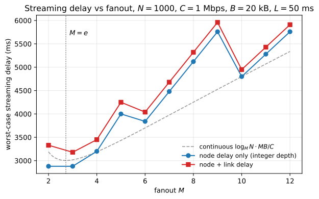
Worst-case streaming delay against fanout \(M\) for a balanced \(M\)-ary multicast tree with \(N=1000\) nodes. The dashed curve is the continuous model \(\log_M N \cdot MB/C\), minimised at \(M=e\); the solid curves use the exact integer depth \(\lceil \log_M(N(M-1)+1)\rceil - 1\), which produces the sawtooth. Small fanouts win: the per-hop cost grows linearly in \(M\) while the depth saving is only logarithmic.
Problem 15.3 — Stable marriage matching
Stable marriage matching. The stable marriage matching problem is an extensively-studied problem and has many applications, from matching medical students to hospitals to analyzing voting systems and auctions. Figure 15.10 illustrates a matching in a bipartite graph: the left column holds nodes 1, 2, 3 and the right column holds nodes 4, 5, 6, and the matching consists of the three disjoint edges \(1 - 6\), \(2 - 4\), and \(3 - 5\), i.e. nodes 1, 2 and 3 are assigned to nodes 6, 4, and 5 respectively. We saw a type of matching, the maximum weight matching, in VCG auctions in Chapter 2.
Suppose a set of partners can be split into two equal-sized subsets \(A\) and \(B\). Each element \(a \in A\) has a strict ranking of potential partners \(b \in B\) (and vice versa). A stable matching assigns each \(a \in A\) to some \(b \in B\) and each \(b \in B\) to some \(a \in A\), such that there does not exist a pair \((a,b) \in A \times B\) with \(a\) preferring \(b\) to the \(b^{\prime} \in B\) that \(a\) is currently assigned to, and \(b\) preferring \(a\) to the \(a^{\prime} \in A\) that \(b\) is currently assigned to (for that would have been two unstable marriages).
A standard solution to the stable marriage matching problem is the Gale–Shapley algorithm. It follows a simple, iterative procedure. A man (a node in set \(A\)), or a woman (a node in set \(B\)), can be unengaged, engaged, or married. In each round, an unengaged man proposes to the most preferred woman among those to whom he has not yet proposed in previous rounds, and each woman chooses to become engaged to the suitor whom she prefers most and rejects the rest. As the iteration continues, engagements may be broken. When there is no longer an unengaged man, the iteration stops, and the engaged pairs at that point are married.
(a) Run the algorithm to find a stable matching between the two sets \(A = \{a,b,c\}\) and \(B = \{d,e,f\}\) with the following rankings: \[ a: d > e > f, \qquad b: d > e > f, \qquad c: d > f > e, \] \[ d: c > b > a, \qquad e: c > a > b, \qquad f: a > c > b. \]
(b) Argue that, at the conclusion of the algorithm, a stable marriage matching must have been found. (difficulty: \(\star\star\star\))
(a) The stable matching is \((a,e)\), \((b,f)\), \((c,d)\).
- Round 1: all three men propose to \(d\), who ranks \(c > b > a\) and keeps \(c\).
- Round 2: \(a\) and \(b\) propose to \(e\), who ranks \(c > a > b\) and keeps \(a\). She would prefer \(c\), but he never proposes, holding \(d\).
- Round 3: \(b\), rejected twice, proposes to \(f\), who is unengaged and accepts although she ranks him last.
Stability needs only the men’s lists above their partners: \(a\) prefers only \(d\), who holds \(c\) above him; \(b\) prefers \(d\) and \(e\), who rank him below their partners; \(c\) has his first choice. No blocking pair.
(b) Three facts, all from the two monotonicities — a man’s proposals move strictly down his list, a woman’s engagement strictly up hers.
- (i) Termination. No man proposes twice to the same woman, so at most \(n^2\) proposals occur, and every round with an unengaged man has at least one.
- (ii) Perfect matching. An engaged woman stays engaged, swapping only upward. If the algorithm halted with \(a\) unmatched, the stopping rule forces \(a\) to have been rejected by all \(n\) women, each engaged at the moment of rejection and hence at the end; so all \(n\) women are married to \(n\) distinct men, accounting for \(a\) too — a contradiction.
- (iii) No blocking pair. Suppose \((a,b)\) blocks, with \(a\) married to \(b^{\prime}\) but preferring \(b\), and \(b\) married to \(a^{\prime}\) but preferring \(a\). Proposing in decreasing order, \(a\) passed \(b\) on the way down to \(b^{\prime}\), so he proposed to her; she either rejected him for a man she preferred or dropped him later for one, so immediately afterwards she was engaged above \(a\). Her partner only improves, so \(a^{\prime}\) is strictly better than \(a\), contradicting the assumption. \(\blacksquare\)
The result is the men-optimal stable matching: every man gets the best partner he has in any stable matching and every woman her worst, so the proposing side holds the advantage.
The code runs the round-based algorithm, then brute-forces all \(3! = 6\) perfect matchings with their blocking pairs:
import itertools
men_pref = {'a': ['d', 'e', 'f'], 'b': ['d', 'e', 'f'], 'c': ['d', 'f', 'e']}
women_pref = {'d': ['c', 'b', 'a'], 'e': ['c', 'a', 'b'], 'f': ['a', 'c', 'b']}
rank = {w: {m: i for i, m in enumerate(p)} for w, p in women_pref.items()}
def gale_shapley():
free = list(men_pref)
nxt = {m: 0 for m in men_pref}
engaged = {} # woman -> man
rnd = 0
while free:
rnd += 1
proposals = {}
for m in list(free):
w = men_pref[m][nxt[m]]
nxt[m] += 1
proposals.setdefault(w, []).append(m)
print('round %d proposals: %s'
% (rnd, {w: sorted(v) for w, v in sorted(proposals.items())}))
for w, suitors in proposals.items():
pool = suitors + ([engaged[w]] if w in engaged else [])
best = min(pool, key=lambda m: rank[w][m])
for m in pool:
if m != best and m not in free:
free.append(m)
engaged[w] = best
for m in suitors:
if m == best:
free.remove(m)
print(' engagements : %s' % {w: engaged[w] for w in sorted(engaged)})
return {m: w for w, m in engaged.items()}
match = gale_shapley()
print('stable matching :', {m: match[m] for m in sorted(match)})
def blocking(match):
inv = {w: m for m, w in match.items()}
bad = []
for m, w in itertools.product(men_pref, women_pref):
if match[m] == w:
continue
if men_pref[m].index(w) < men_pref[m].index(match[m]) and \
rank[w][m] < rank[w][inv[w]]:
bad.append((m, w))
return bad
print('blocking pairs :', blocking(match))
print()
print('all 6 matchings, blocking pairs of each:')
for perm in itertools.permutations('def'):
mm = dict(zip('abc', perm))
print(' ', mm, '->', blocking(mm) or 'STABLE')
round 1 proposals: {'d': ['a', 'b', 'c']}
engagements : {'d': 'c'}
round 2 proposals: {'e': ['a', 'b']}
engagements : {'d': 'c', 'e': 'a'}
round 3 proposals: {'f': ['b']}
engagements : {'d': 'c', 'e': 'a', 'f': 'b'}
stable matching : {'a': 'e', 'b': 'f', 'c': 'd'}
blocking pairs : []
all 6 matchings, blocking pairs of each:
{'a': 'd', 'b': 'e', 'c': 'f'} -> [('b', 'd'), ('c', 'd')]
{'a': 'd', 'b': 'f', 'c': 'e'} -> [('b', 'd'), ('c', 'd'), ('c', 'f')]
{'a': 'e', 'b': 'd', 'c': 'f'} -> [('c', 'd')]
{'a': 'e', 'b': 'f', 'c': 'd'} -> STABLE
{'a': 'f', 'b': 'd', 'c': 'e'} -> [('c', 'd')]
{'a': 'f', 'b': 'e', 'c': 'd'} -> [('a', 'e')]
The exhaustive scan shows that \(\{(a,e),(b,f),(c,d)\}\) is not merely one stable matching but the only one for this instance, so here the men-optimal and women-optimal matchings coincide.
Problem 15.4 — BitTorrent as a game
BitTorrent as a game. BitTorrent’s upload-incentive mechanism can be analyzed with game theory. Let there be \(N\) peers indexed \(1,2,\dots,N\), and let \(c_i\), \(u_i\), and \(d_i\) be peer \(i\)’s upload capacity, upload speed, and download speed, respectively (all in Mbps). The speeds \(u_i\) and \(d_i\) can vary with time. We assume peers have unlimited download capacities.
Each peer \(i\) can directly control its \(u_i\) (constrained by \(u_i \le c_i\)) but not its \(d_i\), and its aim is to maximize \(d_i\) and to minimize \(u_i\). There is a tradeoff between the two objectives: if peer \(i\) makes \(u_i\) small, other peers will realize that peer \(i\) is selfish, and refuse to upload to it, resulting in a small \(d_i\). BitTorrent’s peer-selection mechanism aims to enforce this tradeoff so as to make \(u_i\) large and to encourage uploads.
Now consider the following set of rules, which are a simplified version of BitTorrent’s peer-selection mechanism.
(1) Peers take turns to update \(u_i\) in the ascending order of \(i\) and then wrap around, e.g., \(u_1, u_2, u_3, u_1, u_2, u_3, \dots\) for three users.
(2) When peer \(i\) updates its \(u_i\), all other peers see this change, and choose to upload to the top \(n_u\) (an integral parameter) peers in terms of the \(u_j\) values (and break ties by choosing randomly). The upload speeds are shared evenly among the \(n_u\) peers.
(3) Peer \(i\) chooses \(u_i\) by anticipating the \(d_i\) it receives according to rule (2): \(u_i\) is chosen to maximize the expected \(d_i\). If multiple \(u_i\) values result in the same \(d_i\), choose the smallest one. Then add a small constant \(\epsilon\).
Here come your two tasks in this homework problem. Let there be \(N = 4\) peers with each peer uploading to \(n_u = 2\) peers, and set \(\epsilon = 0.1\).
(a) Suppose \(c_1 = 1\) and \(c_2 = c_3 = c_4 = 2\). Initially it is peer 1’s turn to update \(u_1\) with \(u_2 = u_3 = u_4 = 1.1\). We have the following line of reasoning. (i) Regardless of the value of \(u_1\), no peer will upload to peer 1 (\(d_1 = 0\)) because \(0 \le u_1 \le c_1 < u_2, u_3, u_4\), so peer 1 sets \(u_1 = 0 + \epsilon = 0.1\) by rule (3). (ii) In the next timeslot, it is peer 2’s turn to update \(u_2\), which becomes \(u_1 + \epsilon\) because \(u_2\) needs to be the third largest, i.e., greater than \(u_1\), so that peers 3 and 4 will upload to it. Continue this line of reasoning to show that the \(u_i\) values never converge to fixed values.
(b) Suppose now \(c_1 = c_2 = c_3 = c_4 = 2\). Show that setting \(u_1 = u_2 = u_3 = u_4 = 2\) constitutes a Nash equilibrium. You may first show that, if it is peer \(i\)’s turn to set \(u_i\), setting \(u_i\) to be any value other than \(c_i = 2\) will not improve \(d_i\).
(For more detail, see D. Qiu and R. Srikant, “Modeling and performance analysis of BitTorrent-like peer-to-peer networks,” in Proceedings of ACM Sigcomm, 2004.) (difficulty: \(\star\star\))
With \(N = 4\), \(n_u = 2\), peer \(j\) drops exactly one peer, the minimum of \(\{u_k : k \ne j\}\), so peer \(i\) is refused by \(j\) precisely when \(u_i\) is the least of \(\{u_i\} \cup \{u_k : k \ne i,j\}\). Ranking \(u_{(1)} \ge \cdots \ge u_{(4)}\), this is a two-step ladder: ranks 1 and 2 receive from all three others, \(d = \tfrac12\sum_{j\ne i}u_j\); rank 3 is dropped only by rank 4, so \(d = \tfrac12(u_{(1)}+u_{(2)})\); rank 4 gets nothing. Sorting the others \(a \ge b \ge c\), the mover earns \((a+b+c)/2\) for \(u_i > b\), \((a+b)/2\) for \(b \ge u_i > c\), and 0 for \(u_i < c\).
The two top rungs differ by only \(c/2\), which is \(O(\epsilon)\) when the weakest other peer is a free-rider parked at \(\epsilon\); the printed step (ii) treats that as no improvement, invoking rule (3)’s “choose the smallest” tie-break, and I follow it. The best response is then \[ u_i \;=\; \begin{cases} \min\{c + \epsilon,\, c_i\}, & c \le \epsilon,\; c_i > c,\\[2pt] \min\{b + \epsilon,\, c_i\}, & c > \epsilon,\; c_i > b,\\[2pt] \min\{c + \epsilon,\, c_i\}, & c > \epsilon,\; b \ge c_i > c,\\[2pt] \epsilon, & c_i \le c, \end{cases} \] valid whenever the mover can place itself strictly on a rung; a fully tied profile needs rule (2)’s random tie-break directly, which is part (b).
(a) The orbit is periodic with period 24 and has no fixed point. Step (i) is the last case: \(c_1 = 1 < 1.1\), so \(d_1 = 0\) always and peer 1 free-rides at \(0.1\). Step (ii) is the first case: peer 2 sees \(c = u_1 = \epsilon\), so third place pays \(1.1\) against the top two’s \(1.15\), a gap of only \(u_1/2 = \epsilon/2\), and it takes the cheap seat at \(0.2\). Peers 3 and 4 do likewise, giving \((0.1, 0.2, 0.2, 0.2)\). At timeslot 5 no free-rider remains, so the second rung’s \(c/2 = 0.1\) is an \(O(1)\) gain and peer 1 climbs to \(b + \epsilon = 0.3\); thereafter each mover plays the median of the others plus \(\epsilon\) and the group ratchets up: \[ (0.3, 0.2, 0.2, 0.2) \to (0.3, 0.3, 0.2, 0.2) \to (0.3, 0.3, 0.4, 0.2) \to (0.3, 0.3, 0.4, 0.4) \to \cdots \] No state is fixed, since the mover always lands strictly above the others’ minimum, so that minimum strictly increases at least once every four timeslots. The climb pushes the others’ median past \(c_1 = 1\) at timeslot 25, profile \((1.0, 1.1, 1.1, 1.2)\), where peer 1 can afford neither second nor third place and rule (3) returns it to \(\epsilon\); peers 2–4 collapse to \(0.2\) and timeslot 29 reproduces timeslot 5. Peers 2–4 never exceed \(1.2\), so their capacity never binds: the asymmetry \(c_1 = 1 < 2\) alone manufactures the cycle, and a bounded orbit on the \(\epsilon\)-grid with no fixed point must be eventually periodic.
This depends on treating \(\epsilon\)-order crumbs as negligible. Maximizing \(d_i\) literally at \(\epsilon = 0.1\) makes every capable peer strictly prefer the top two, and \((\epsilon, 2, 2, 2)\) becomes a genuine fixed point, where peer 2 collects \(2 + \epsilon/3\) from the three-way tie against third place’s \(2\) (second code block). The printed step (ii) commits to the leading-order model used above.
(b) Yes. With \(c_i = 2\) for all \(i\), at \(u = (2,2,2,2)\) every \(j\) faces a three-way tie and draws a uniform pair, selecting \(i\) with probability \(\binom{2}{1}/\binom{3}{2} = 2/3\) at \(u_j/n_u = 1\) each:
\[ \mathbb{E}[d_i] \;=\; \sum_{j \ne i} \frac{2}{3} \cdot \frac{2}{2} \;=\; 3 \cdot \frac{2}{3} \;=\; 2 \text{ Mbps}. \]
Any deviation to \(u_i < 2\) makes \(u_i\) the strict minimum of the triple \(\{u_i, 2, 2\}\) that every \(j \ne i\) ranks, so all three drop it and \(d_i = 0\); deviating upward is infeasible. Hence \(u_i = 2\) uniquely maximizes \(d_i\) on \([0,c_i]\), the payoff falling discontinuously from 2 to 0 at any shaving, so under the model’s lexicographic objective it is the strict best response and \((2,2,2,2)\) is a Nash equilibrium. \(\blacksquare\) (Rule (3) is stationary here, since \(2 + \epsilon\) exceeds capacity.)
So heterogeneity, not selfishness, breaks this mechanism: peer 1 contributes willingly whenever the ladder is low enough, but each ejection plants a free-rider at the bottom rung, which is exactly what makes third place as good as second for everyone else.
import itertools
import numpy as np
def expected_d(u, i, nu=2):
"""Exact E[d_i] under rule (2): peer j splits u_j evenly over the top-nu
peers among the others, ties broken uniformly at random."""
tot = 0.0
for j in range(len(u)):
if j == i:
continue
cand = [k for k in range(len(u)) if k != j]
subsets = list(itertools.combinations(cand, nu))
best = max(sum(u[k] for k in S) for S in subsets)
win = [S for S in subsets if abs(sum(u[k] for k in S) - best) < 1e-12]
tot += sum(1 for S in win if i in S) / len(win) * u[j] / nu
return tot
def best_response(u, i, cap, eps=0.1):
"""Rule (3) to leading order in eps: take the cheapest rung whose download
is maximal, counting two downloads that differ by O(eps) as the same,
then add eps and clip at capacity."""
a, b, c = sorted((u[k] for k in range(len(u)) if k != i), reverse=True)
opts = [(0.0, 0.0)] # last place: d_i = 0
if cap[i] > c:
opts.append((c, (a + b) / 2)) # third place
if cap[i] > b:
opts.append((b, (a + b + c) / 2)) # top two
top = max(p for _, p in opts)
thr = min(t for t, p in opts if p >= top - eps / 2 - 1e-12)
return round(min(thr + eps, cap[i]), 6)
print('peer 2 facing (u1,u3,u4) = (0.1, 1.1, 1.1), exact E[d2]:')
for x in [0.05, 0.2, 1.0, 1.1, 1.2, 2.0]:
print(' u2 = %4.2f E[d2] = %.4f' % (x, expected_d([0.1, x, 1.1, 1.1], 1)))
print(' gap between third place and top two = %.2f = eps/2'
% (expected_d([0.1, 1.2, 1.1, 1.1], 1) - expected_d([0.1, 0.2, 1.1, 1.1], 1)))
print()
cap = [1.0, 2.0, 2.0, 2.0]
u = [0.0, 1.1, 1.1, 1.1]
hist = []
for t in range(200):
u[t % 4] = best_response(u, t % 4, cap)
hist.append(list(u))
arr = np.array(hist)
print(' t turn u1 u2 u3 u4')
for t in list(range(8)) + list(range(20, 30)):
print(' %2d peer %d %5.2f %5.2f %5.2f %5.2f' % (t + 1, t % 4 + 1, *arr[t]))
seen = {}
for t in range(0, 200, 4):
key = tuple(np.round(arr[t], 3))
if key in seen:
print()
print('limit cycle: state at turn %d recurs at turn %d, period %d timeslots'
% (seen[key] + 1, t + 1, t - seen[key]))
break
seen[key] = t
print('collapses of u2 (drop of more than 0.5) at turns:',
[t + 1 for t in range(1, 100) if arr[t, 1] < arr[t - 1, 1] - 0.5])
print('is any four-turn round a fixed point? ',
any(np.allclose(arr[t], arr[t + 4]) for t in range(len(arr) - 4)))
print('highest u ever reached by peers 2-4: %.1f (capacity 2 is never binding)'
% arr[:, 1:].max())
print()
print('part (b), all capacities 2: E[d_i] at u = (2,2,2,2) is', round(expected_d([2.] * 4, 0), 6))
for x in [0.0, 1.0, 1.9, 1.99, 2.0]:
print(' peer 1 deviates to u1 = %5.3f -> E[d1] = %.4f'
% (x, expected_d([x, 2, 2, 2], 0)))
peer 2 facing (u1,u3,u4) = (0.1, 1.1, 1.1), exact E[d2]:
u2 = 0.05 E[d2] = 0.0000
u2 = 0.20 E[d2] = 1.1000
u2 = 1.00 E[d2] = 1.1000
u2 = 1.10 E[d2] = 1.1333
u2 = 1.20 E[d2] = 1.1500
u2 = 2.00 E[d2] = 1.1500
gap between third place and top two = 0.05 = eps/2
t turn u1 u2 u3 u4
1 peer 1 0.10 1.10 1.10 1.10
2 peer 2 0.10 0.20 1.10 1.10
3 peer 3 0.10 0.20 0.20 1.10
4 peer 4 0.10 0.20 0.20 0.20
5 peer 1 0.30 0.20 0.20 0.20
6 peer 2 0.30 0.30 0.20 0.20
7 peer 3 0.30 0.30 0.40 0.20
8 peer 4 0.30 0.30 0.40 0.40
21 peer 1 1.00 0.90 1.00 1.00
22 peer 2 1.00 1.10 1.00 1.00
23 peer 3 1.00 1.10 1.10 1.00
24 peer 4 1.00 1.10 1.10 1.20
25 peer 1 0.10 1.10 1.10 1.20
26 peer 2 0.10 0.20 1.10 1.20
27 peer 3 0.10 0.20 0.20 1.20
28 peer 4 0.10 0.20 0.20 0.20
29 peer 1 0.30 0.20 0.20 0.20
30 peer 2 0.30 0.30 0.20 0.20
limit cycle: state at turn 5 recurs at turn 29, period 24 timeslots
collapses of u2 (drop of more than 0.5) at turns: [2, 26, 50, 74, 98]
is any four-turn round a fixed point? False
highest u ever reached by peers 2-4: 1.2 (capacity 2 is never binding)
part (b), all capacities 2: E[d_i] at u = (2,2,2,2) is 2.0
peer 1 deviates to u1 = 0.000 -> E[d1] = 0.0000
peer 1 deviates to u1 = 1.000 -> E[d1] = 0.0000
peer 1 deviates to u1 = 1.900 -> E[d1] = 0.0000
peer 1 deviates to u1 = 1.990 -> E[d1] = 0.0000
peer 1 deviates to u1 = 2.000 -> E[d1] = 2.0000
Turn 25 is peer 1’s exit, 26–28 the collapse, and 29 reproduces turn 5. Part (b)’s rows show the payoff cliff: every deviation below 2 gives exactly zero. Removing the \(O(\epsilon)\) tolerance instead makes the dynamics convergent:
def best_response_literal(u, i, cap, eps=0.1):
"""Same rule but with no O(eps) tolerance: maximise E[d_i] exactly."""
grid = sorted(set(list(np.round(np.arange(0, cap[i] + 1e-9, 0.05), 4))
+ [min(u[k], cap[i]) for k in range(len(u)) if k != i]))
vals = []
for x in grid:
v = list(u)
v[i] = x
vals.append(expected_d(v, i))
top = max(vals)
thr = min(x for x, val in zip(grid, vals) if val > top - 1e-12)
return round(min(thr + eps, cap[i]), 6)
u = [0.0, 1.1, 1.1, 1.1]
lit = []
for t in range(120):
u[t % 4] = best_response_literal(u, t % 4, cap)
lit.append(list(u))
lit = np.array(lit)
print('literal-eps variant, every fourth turn:')
for t in range(0, 48, 4):
print(' turn %3d : %5.2f %5.2f %5.2f %5.2f' % (t + 1, *lit[t]))
print(' ...')
print(' turn %3d : %5.2f %5.2f %5.2f %5.2f' % (120, *lit[-1]))
print('fixed point reached?', bool(np.allclose(lit[-1], lit[-9])))
literal-eps variant, every fourth turn:
turn 1 : 0.10 1.10 1.10 1.10
turn 5 : 0.10 1.25 1.25 1.40
turn 9 : 0.10 1.40 1.55 1.55
turn 13 : 0.10 1.70 1.70 1.85
turn 17 : 0.10 1.85 2.00 2.00
turn 21 : 0.10 2.00 2.00 2.00
turn 25 : 0.10 2.00 2.00 2.00
turn 29 : 0.10 2.00 2.00 2.00
turn 33 : 0.10 2.00 2.00 2.00
turn 37 : 0.10 2.00 2.00 2.00
turn 41 : 0.10 2.00 2.00 2.00
turn 45 : 0.10 2.00 2.00 2.00
...
turn 120 : 0.10 2.00 2.00 2.00
fixed point reached? True
(The \(0.05\) grid step explains the intermediate values.) Under the literal reading the profile settles at \((\epsilon,2,2,2)\), so the claimed non-convergence is a leading-order statement.
import matplotlib.pyplot as plt
fig, ax = plt.subplots(figsize=(8, 4))
T = 56
for i, col in enumerate(['#d62728', '#1f77b4', '#2ca02c', '#9467bd']):
ax.step(range(1, T + 1), arr[:T, i], where='post', color=col, lw=1.6,
label='$u_%d$ ($c_%d=%.0f$)' % (i + 1, i + 1, cap[i]))
ax.axhline(1.0, color='0.5', ls=':', lw=1)
for x in (5, 29, 53):
ax.axvline(x, color='0.8', lw=0.8)
ax.set_xlabel('timeslot (peers update in the order 1,2,3,4,1,2,...)')
ax.set_ylabel('upload speed $u_i$ (Mbps)')
ax.set_title('Best-response dynamics never settle: $c=(1,2,2,2)$, $n_u=2$, $\\epsilon=0.1$')
ax.legend(frameon=False, fontsize=9, ncol=4, loc='upper center')
ax.set_ylim(-0.1, 1.7)
ax.grid(alpha=0.3)
plt.savefig('nl-ch15-bittorrent-cycle.svg', dpi=150, bbox_inches='tight')
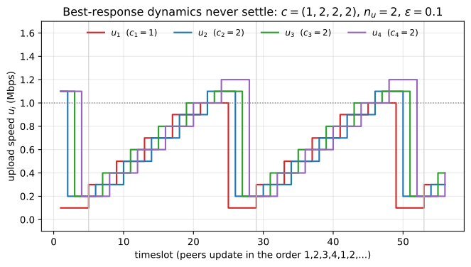
Best-response dynamics of the simplified BitTorrent peer-selection game with \(c = (1,2,2,2)\), \(n_u = 2\), \(\epsilon = 0.1\). All four peers leapfrog each other upward in steps of \(\epsilon\) until the ladder rises past peer 1’s capacity of 1 Mbps (dotted line); peer 1 (red) then drops to \(u_1 = \epsilon\), which makes third place as cheap and as good as second for everyone else, and peers 2–4 collapse to \(0.2\) before the climb restarts. The vertical rules at timeslots 5, 29 and 53 mark the repeats: the orbit is periodic with period 24 and has no fixed point. Note that the capacity of 2 Mbps shared by peers 2–4 is never reached.
Problem 15.5 — Private torrent games
Private torrent games. We have been discussing the public BitTorrent. There are also many private torrents that create their own rules of rewarding seeders and encouraging uploads beyond the simple tit-for-tat in BitTorrent. More than 800 such private communities were found in 2009. In this homework problem, we explore one possible rule of proportional reward, again through the modeling language of game theory and utility functions.
Let \(d_i\) and \(u_i\) be the actual download and upload volumes, now measured in bytes, for peer \(i\) in a fixed population of peers. A standard incentive mechanism in private BitTorrents is the following ratio incentive: \[ d_i \le f(u_i), \] i.e., the download volume cannot be bigger than some function of the upload volume. An affine parameterization of this function is \[ f(u_i) = \frac{u_i}{\theta} + \Delta. \] Here, as in the leaky-bucket admission control that we will see in Chapter 17, \(\theta\) is the upload–download ratio targeted, and \(\Delta\) is the slack: the amount of data a peer can download outside of the ratio rule.
Each peer’s net utility function \(V_i\) (we use \(V\) instead of \(U\) here, since \(U\) is already used to denote “upload”) can be parameterized as follows: \[ V_i(d_i, u_i) = B(d_i) - C(u_i) + \beta\bigl(f(u_i) - d_i\bigr), \] as long as \(f(u_i) - d_i \ge 0\). It becomes \(-\infty\) (meaning that it will be evicted from the community) otherwise. Here, \(B\) and \(C\) are some utility and cost functions, and \(\beta\) is a positive weight.
Suppose the strategy for peer \(i\) is the two-tuple of target download and target upload (per unit time): \((\delta_i, \sigma_i)\), over the strategy spaces of \(\delta_i \in [0,D]\) and \(\sigma_i \in [0,U]\).
(a) How can we express the actual upload and download amounts \(\{u_i, d_i\}\) as functions of the strategies \(\{\delta_i, \sigma_i\}\) chosen by all the peers? This can be very difficult, but if we make an assumption that all the downloads add up to be exactly the same as the sum of all the uploads, then there is a closed-form answer. What is that answer?
(b) Now we want the Nash equilibrium to be efficient: each peer chooses the target download and upload to be just \(D\) and \(U\). Prove that \((\delta_i, \sigma_i) = (D,U)\), \(\forall i\), is indeed a Nash equilibrium if \(f(u) > u\) and \(f^{\prime}(u) > C^{\prime}(u)/\beta\). (Hint: You can assume that all users have upload and download capacities \(U\) and \(D\) except possibly user \(i\). This will simplify the expression found in (a).)
(c) As a corollary to part (b), show that if the ratio incentive parameters \((\theta, \Delta)\) are such that \(u/\theta + \Delta > u\) and \(\beta > \theta C^{\prime}(u)\) for all \(u \in [0,U]\), then using a ratio incentive implies that \((\delta_i, \sigma_i) = (D,U)\), \(\forall i\), is the unique Nash equilibrium. (Hint: Assume that each user except user \(i\) follows the same strategy, and argue in three separate cases of that strategy.)
(For more details, see Z. Liu, P. Dhungel, D. Wu, C. Zhang, and K. W. Ross, “Understanding and improving incentives in private P2P communities,” in Proceedings of IEEE International Conference on Distributed Computing Systems, 2010.) (difficulty: \(\star\star\star\))
(a) With \(\mathcal{D} = \sum_j \delta_j\) and \(\mathcal{S} = \sum_j \sigma_j\), \[ \boxed{\;d_i = \delta_i \min\left\{1, \frac{\mathcal{S}}{\mathcal{D}}\right\}, \qquad u_i = \sigma_i \min\left\{1, \frac{\mathcal{D}}{\mathcal{S}}\right\}. \;} \] Three conditions force this. No peer exceeds its own target, so \(\sum_j d_j = \sum_j u_j =: \mathcal{T} \le \min\{\mathcal{D},\mathcal{S}\}\); the swarm is not deliberately idle, so the short side sets \(\mathcal{T} = \min\{\mathcal{D},\mathcal{S}\}\); and rationing is anonymous, so \(d_i/\delta_i\) and \(u_i/\sigma_i\) are constant across peers. Then \(\sum_i d_i = \min\{\mathcal{D},\mathcal{S}\} = \sum_i u_i\) (Check!). Supply-limited (\(\mathcal{D} > \mathcal{S}\), the usual case since \(D > U\)) means everyone uploads its target and downloads scale by \(\mathcal{S}/\mathcal{D}\); demand-limited swaps the roles.
Fixing the others, \(d_i\) strictly increases in \(\delta_i\) and \(u_i\) in \(\sigma_i\): supply-limited,
\[ \frac{\partial d_i}{\partial \delta_i} = \frac{\mathcal{S}(\mathcal{D} - \delta_i)}{\mathcal{D}^2} > 0, \qquad \frac{\partial u_i}{\partial \sigma_i} = 1, \]
and demand-limited, \[ \frac{\partial d_i}{\partial \delta_i} = 1, \qquad \frac{\partial u_i}{\partial \sigma_i} = \frac{\mathcal{D}(\mathcal{S} - \sigma_i)}{\mathcal{S}^2} > 0, \] returns diminishing on the rationed side because raising your target dilutes the pool.
(b) Fix all \(j \ne i\) at \((D,U)\), with \(D \ge U\) (asymmetric access, Section 15.4.1). Then \(\mathcal{D} \ge (N-1)D\) and \(\mathcal{S} \le NU\), so for large \(N\) the swarm is supply-limited and \[ u_i = \sigma_i, \qquad d_i = \delta_i \cdot \frac{(N-1)U + \sigma_i}{(N-1)D + \delta_i}. \] At the candidate profile \(\mathcal{D} = ND\), \(\mathcal{S} = NU\), so \(d_i = U = u_i\): conservation plus symmetry forces each peer to download what it uploads, and this is where \(f(u) > u\) first enters, making the eviction constraint \(d_i = U \le f(U)\) slack. Differentiating the payoff,
\[ V_i = B(d_i) - C(u_i) + \beta\bigl(f(u_i) - d_i\bigr), \] \[ \frac{\partial V_i}{\partial \sigma_i} = \underbrace{\bigl(\beta f^{\prime}(u_i) - C^{\prime}(u_i)\bigr)}_{>\,0 \text{ by assumption}} \cdot \underbrace{\frac{\partial u_i}{\partial \sigma_i}}_{>\,0} \;+\; \bigl(B^{\prime}(d_i) - \beta\bigr)\underbrace{\frac{\partial d_i}{\partial \sigma_i}}_{\ge\,0}, \] \[ \frac{\partial V_i}{\partial \delta_i} = \bigl(B^{\prime}(d_i) - \beta\bigr)\underbrace{\frac{\partial d_i}{\partial \delta_i}}_{>\,0}. \]
The upload direction is exactly the stated hypothesis \(\beta f^{\prime}(u) > C^{\prime}(u)\): a marginal uploaded byte buys more ratio credit, valued at \(\beta\), than it costs, so \(V_i\) increases in \(\sigma_i\) and \(\sigma_i = U\). The download direction needs \(B^{\prime}(d) > \beta\) on \([0,D]\), which the printed hypotheses omit — neither mentions \(B\) — so I assume it: without it a peer hoards credit rather than using it and its best response is an interior \(\delta_i < D\), a failure the code below exhibits at large \(\beta\). With both signs, \(V_i\) strictly increases in each coordinate on the feasible set, and \((D,U)\) is feasible since \(d_i = U < f(U)\), so it is peer \(i\)’s strict best response and the profile is a Nash equilibrium. \(\blacksquare\)
(c) With \(f(u) = u/\theta + \Delta\), \(f^{\prime} = 1/\theta\), so the hypotheses of (b) are exactly the stated parameter conditions:
\[ f(u) > u \iff \frac{u}{\theta} + \Delta > u, \qquad f^{\prime}(u) > \frac{C^{\prime}(u)}{\beta} \iff \frac{\beta}{\theta} > C^{\prime}(u) \iff \beta > \theta C^{\prime}(u), \] for all \(u \in [0,U]\), so (b) applies. Following the hint, let every peer but \(i\) play a common \((\delta,\sigma)\), so \(\mathcal{D} \approx N\delta\), \(\mathcal{S} \approx N\sigma\); the two sign facts of (b) hold at every operating point, so \(V_i\) strictly increases in both coordinates wherever feasible. Three cases by the sign of \(\delta - \sigma\):
- (i) \(\delta < \sigma\) (excess supply): \(d_i = \delta_i\), \(u_i = \sigma_i\mathcal{D}/\mathcal{S}\). If \(\sigma < U\), raising \(\sigma_i\) gains. If \(\sigma = U\) then \(\delta < U \le D\) and the eviction constraint \(\delta \le f(\delta)\) is slack by \(f(u) > u\), so raising \(\delta_i\) gains.
- (ii) \(\delta = \sigma\): \(d_i = \delta_i\), \(u_i = \sigma_i\). Again \(\sigma < U\) is beaten by raising \(\sigma_i\); and \(\sigma = U\) leaves \(\delta = U < D\) with feasibility up to \(f(U) > U\), so raising \(\delta_i\) gains.
- (iii) \(\delta > \sigma\) (excess demand): \(u_i = \sigma_i\), \(d_i = \delta_i\mathcal{S}/\mathcal{D}\). So \(\sigma = U\); and if \(\delta < D\), feasibility \(\delta_i\sigma/\delta \le f(U)\) permits \(\delta_i\) up to \(\delta f(U)/U > \delta\), a strict gain. Hence \(\delta = D\).
Every case forces \((D,U)\), which (b) confirms is an equilibrium, so it is unique within the hint’s class. \(\blacksquare\) Unlike Problem 15.4’s rank-threshold rule, the private-tracker rule is smooth in \(u_i\), and that smoothness buys uniqueness.
Taking \(N = 50\), \(D = 10\), \(U = 4\), \(\theta = 1.5\), \(\Delta = 6\), \(B(d) = 60\ln(1+d)\), \(C(u) = u^2/4\), so that \(f(u) - u = 6 - u/3 > 0\) and both conditions hold at \(\beta = 4\), the code brute-forces peer 1’s best response:
import numpy as np
N, D, U = 50, 10.0, 4.0
theta, slack = 1.5, 6.0
b0, gamma = 60.0, 0.5
f, fp = (lambda u: u / theta + slack), (lambda u: 1.0 / theta)
B, Bp = (lambda d: b0 * np.log(1 + d)), (lambda d: b0 / (1 + d))
C, Cp = (lambda u: 0.5 * gamma * u ** 2), (lambda u: gamma * u)
def realized(delta, sigma):
"""Part (a): proportional rationing on the short side, so sum d = sum u."""
Dt, St = max(np.sum(delta), 1e-12), max(np.sum(sigma), 1e-12)
return delta * min(1.0, St / Dt), sigma * min(1.0, Dt / St)
def V(di, ui, beta):
return -np.inf if f(ui) - di < 0 else B(di) - C(ui) + beta * (f(ui) - di)
def best_response(beta, others=(D, U), n=201):
delta, sigma = np.full(N, others[0]), np.full(N, others[1])
best, arg = -np.inf, None
for x in np.linspace(0, D, n):
for y in np.linspace(0, U, n):
delta[0], sigma[0] = x, y
d, u = realized(delta, sigma)
v = V(d[0], u[0], beta)
if v > best:
best, arg = v, (x, y)
return arg, best
d, u = realized(np.full(N, D), np.full(N, U))
print('all %d peers play (D,U) = (%.0f, %.0f):' % (N, D, U))
print(' realized d_i = %.3f, u_i = %.3f, sum d = sum u = %.1f' % (d[0], u[0], d.sum()))
print(' f(u_i) = %.3f > u_i = %.3f, so no eviction (slack %.3f)'
% (f(u[0]), u[0], f(u[0]) - u[0]))
print(" min over [0,U] of beta f'(u) - C'(u) at beta = 4 : %+.4f"
% min(4 * fp(x) - Cp(x) for x in np.linspace(0, U, 201)))
print(" min over [0,D] of B'(d) - beta at beta = 4 : %+.4f"
% min(Bp(x) - 4 for x in np.linspace(0, D, 201)))
print()
for beta, tag in [(4.0, 'both conditions hold'),
(2.0, "beta < theta C'(U), so the upload condition fails"),
(20.0, "beta > B'(d), so the download condition fails")]:
arg, val = best_response(beta)
print('beta = %5.1f (%s)' % (beta, tag))
print(' peer 1 best response to everyone else at (D,U): (%.2f, %.2f), V = %.3f'
% (arg[0], arg[1], val))
print()
print('part (c) scan at beta = 4: every peer but 1 plays the same (delta, sigma)')
print(' others peer 1 best response regime')
for od, os in [(10., 4.), (10., 1.), (5., 4.), (5., 1.), (2., 4.), (2., 0.), (1., 4.)]:
arg, _ = best_response(4.0, others=(od, os), n=101)
reg = 'excess demand' if od > os else ('balanced' if od == os else 'excess supply')
print(' (%5.2f, %5.2f) -> (%5.2f, %5.2f) %s' % (od, os, arg[0], arg[1], reg))
all 50 peers play (D,U) = (10, 4):
realized d_i = 4.000, u_i = 4.000, sum d = sum u = 200.0
f(u_i) = 8.667 > u_i = 4.000, so no eviction (slack 4.667)
min over [0,U] of beta f'(u) - C'(u) at beta = 4 : +0.6667
min over [0,D] of B'(d) - beta at beta = 4 : +1.4545
beta = 4.0 (both conditions hold)
peer 1 best response to everyone else at (D,U): (10.00, 4.00), V = 111.233
beta = 2.0 (beta < theta C'(U), so the upload condition fails)
peer 1 best response to everyone else at (D,U): (10.00, 3.06), V = 102.117
beta = 20.0 (beta > B'(d), so the download condition fails)
peer 1 best response to everyone else at (D,U): (4.95, 4.00), V = 195.250
part (c) scan at beta = 4: every peer but 1 plays the same (delta, sigma)
others peer 1 best response regime
(10.00, 4.00) -> (10.00, 4.00) excess demand
(10.00, 1.00) -> (10.00, 4.00) excess demand
( 5.00, 4.00) -> (10.00, 4.00) excess demand
( 5.00, 1.00) -> (10.00, 4.00) excess demand
( 2.00, 4.00) -> ( 7.40, 4.00) excess supply
( 2.00, 0.00) -> (10.00, 4.00) excess demand
( 1.00, 4.00) -> ( 6.70, 4.00) excess supply
With both conditions holding the best response to \((D,U)\) is exactly \((D,U)\), confirming (b); \(\beta\) below \(\theta C^{\prime}(U)\) shaves the upload to \(3.06\), and \(\beta\) above \(B^{\prime}(d)\) shaves the download to \(4.95\) — the second being the failure the printed hypotheses do not cover. In the part (c) scan every row returns \(\sigma_1 = U\) and a \(\delta_1\) strictly above the common \(\delta\), refuting each profile. The two excess-supply rows stop short of \(D\) only because the swarm is demand-starved there, throttling \(u_1\) and making the eviction constraint \(d_1 \le f(u_1)\) bind.
What’s inside the cloud of iCloud?
Problem 16.1 — To cloud or not to cloud
To cloud or not to cloud. The Bumbershoot Corporation’s biology research center produces 600 GB of new data for every wet lab experiment. Assume the data generated can be easily parallelized, with a negligible overhead.
(a) Suppose Amazon Web Services (AWS) sells CPU hours at the price of $0.10 per hour per Elastic Compute Cloud (EC2) instance, where each instance takes 2 hours to process 1 GB of the experimental data. The data-transfer fee is $0.15/GB. What is the price Bumbershoot will need to pay for processing an experiment using the EC2 service?
(b) Suppose the data-transfer rate from the research center to AWS is 20 Mbps. What is the total time required to transmit and process the experimental data using the EC2 service?
(c) The Bumbershoot Corporation has 24 computers itself, each taking 2 hours to process 1 GB of data. Suppose the overall cost (including electricity, software, hardware, etc) is $15 per computer per experiment. What is the total amount of time and cost required to process the experiment? Will Bumbershoot Corporation be willing to use the EC2 service?
(d) We saw in (b) and (c) that the data transmission time can be a problem in cloud computing. Can you think of a way to overcome this obstacle, so that Bumbershoot can still process the experiment using the EC2 service within a day? (difficulty: \(\star\))
(a) $210; (b) 68.7 hours; (c) 50 hours and $360, so EC2 is cheaper but slower; (d) courier the disks.
(a) The work is \(600 \times 2 = 1200\) instance-hours at $0.10 each, and ingress costs \(600 \times 0.15\), so
\begin{equation*} C_{\text{EC2}} = 120 + 90 = \$210 , \end{equation*}
of which 43% is transport rather than computation.
(b) In decimal GB (\(1\ \text{GB} = 8\times10^{9}\) bits) the upload of \(4.8\times10^{12}\) bits at 20 Mbps takes
\begin{align*} T_{\text{up}} &= \frac{4.8\times 10^{12}}{2\times 10^{7}} = 2.4\times 10^{5}\ \text{s} = 66.7\ \text{h},\\ T_{\text{EC2}} &= 66.7 + 2 = 68.7\ \text{h}, \end{align*}
the 2 hours being the compute stage, since the job parallelizes with negligible overhead and 600 on-demand instances each take 1 GB. The link is 97% of the elapsed time.
(c) Splitting the data over the 24 in-house machines,
\begin{equation*} T_{\text{in}} = \frac{600}{24}\times 2 = 50\ \text{h}, \qquad C_{\text{in}} = 24 \times 15 = \$360 . \end{equation*}
EC2 saves $150 per experiment but costs 18.7 extra hours, so Bumbershoot should take it only when results are not urgent: the in-house 50 hours is pure compute that shrinks as machines are added, whereas the EC2 figure is dominated by a link that renting cannot speed up.
(d) Ship the disks. Finishing within a day leaves 22 hours for transfer, i.e. \(4.8\times10^{12}/(22\times3600) = 60.6\) Mbps, three times the installed link; an overnight courier (AWS Import/Export) delivers 600 GB in 12 hours, an effective 111 Mbps, at the price of a courier fee rather than a network upgrade. For a lab running this weekly, compressing or pre-filtering 3x on the in-house machines, and buying a 1 Gbps circuit (1.3 h upload), are the recurring fixes; pipelining transfer against compute removes only the 2-hour term.
D = 600.0 # GB per experiment
cpu_h_per_GB = 2.0
compute_cost = D*cpu_h_per_GB*0.10
xfer_cost = D*0.15
print("EC2 instance-hours :", D*cpu_h_per_GB)
print("EC2 cost ($) : compute %.0f + transfer %.0f = %.0f"
% (compute_cost, xfer_cost, compute_cost+xfer_cost))
bits = D*8e9 # decimal GB -> bits
t_up = bits/20e6
print("upload at 20 Mbps (h) : %.2f (%.2f days)" % (t_up/3600, t_up/86400))
print("EC2 total time (h) : %.2f" % (t_up/3600 + 2.0))
M = 24
print("in-house time (h) : %.1f" % ((D/M)*cpu_h_per_GB))
print("in-house cost ($) : %.0f" % (M*15))
print("rate needed for 24 h (Mbps): %.1f" % (bits/((24-2)*3600)/1e6))
print("upload at 1 Gbps (h) : %.2f" % (bits/1e9/3600))
print("courier, 12 h door-to-door, effective rate (Mbps): %.0f"
% (bits/(12*3600)/1e6))
EC2 instance-hours : 1200.0
EC2 cost ($) : compute 120 + transfer 90 = 210
upload at 20 Mbps (h) : 66.67 (2.78 days)
EC2 total time (h) : 68.67
in-house time (h) : 50.0
in-house cost ($) : 360
rate needed for 24 h (Mbps): 60.6
upload at 1 Gbps (h) : 1.33
courier, 12 h door-to-door, effective rate (Mbps): 111
Problem 16.2 — Ideal throughput
Ideal throughput. Consider an interconnection network on a microprocessor chip, represented by a directed graph \(G = (V,E)\), where \(V = \{v_i : i = 1,\dots,|V|\}\) is the set of nodes representing the terminals and routers on the chip, and \(E = \{e_c : c = 1,\dots,|E|\}\) is the set of links called “channels.” Define the following symbols: \(\lambda_{s,d}\), the traffic from input port \(s\) to destination port \(d\); \(x_{d,c}\), the traffic with destination \(d\) on channel \(c\); \(b_c\), the bandwidth of channel \(c\); \(\gamma_c\), the load of channel \(c\); and \(\mathbf{A}\), the node-channel incidence matrix, where
\begin{equation*} A_{ic} = \begin{cases} +1 & \text{if } c \text{ is an outgoing channel from node } i,\\ -1 & \text{if } c \text{ is an incoming channel to node } i,\\ 0 & \text{otherwise.}\end{cases} \end{equation*}
(a) What is the incidence matrix of the graph in Figure 16.11? Figure 16.11 is a six-node directed graph drawn as a \(3 \times 2\) grid: nodes 1, 3, 5 across the top row (left to right) and nodes 2, 4, 6 across the bottom row, with node \(i\) sitting above node \(i+1\) for \(i = 1,3,5\). Every grid edge carries two oppositely directed channels, numbered as follows. Vertical edges: channel 1 is \(2 \to 1\) and channel 2 is \(1 \to 2\); channel 7 is \(4 \to 3\) and channel 8 is \(3 \to 4\); channel 13 is \(6 \to 5\) and channel 14 is \(5 \to 6\). Top-row horizontal edges: channel 3 is \(3 \to 1\) and channel 4 is \(1 \to 3\); channel 9 is \(5 \to 3\) and channel 10 is \(3 \to 5\). Bottom-row horizontal edges: channel 5 is \(4 \to 2\) and channel 6 is \(2 \to 4\); channel 11 is \(6 \to 4\) and channel 12 is \(4 \to 6\). So \(|V| = 6\) and \(|E| = 14\).
(b) Define
\begin{equation*} f_{d,i} = \begin{cases} \lambda_{i,d} & \text{if } i \neq d,\\ -\sum_{j \neq d} \lambda_{j,d} & \text{if } i = d.\end{cases} \end{equation*}
What is the relationship between \(f_{d,i}\) and \(x_{d,i}\)?
(c) Express the load \(\gamma_c\) in terms of the traffic \(x_{d,c}\).
(d) The ideal throughput \(\Theta^*\) is the maximum throughput achievable in the network. What is the ideal throughput in terms of \(\gamma_c\) and the bandwidth \(b_c\)?
(e) Formulate the optimization problem of maximizing the ideal throughput via flow control (i.e., varying the traffic \(x_{d,i}\)), for a given traffic pattern \(\lambda_{s,d}\) and incidence matrix \(\mathbf{A}\). (difficulty: \(\star\star\))
(a) The \(6\times14\) matrix below; (b) \(\mathbf{A}\mathbf{x}_d = \mathbf{f}_d\); (c) \(\gamma_c = \sum_d x_{d,c}\); (d) \(\Theta^* = \min_c b_c/\gamma_c\); (e) the max-concurrent-flow LP.
(a) Reading the channel numbering off Figure 16.11, each column carries one \(+1\) at its tail and one \(-1\) at its head:
\begin{equation*} \mathbf{A} = \begin{bmatrix} -1 & 1 & -1 & 1 & 0 & 0 & 0 & 0 & 0 & 0 & 0 & 0 & 0 & 0\\ 1 & -1 & 0 & 0 & -1 & 1 & 0 & 0 & 0 & 0 & 0 & 0 & 0 & 0\\ 0 & 0 & 1 & -1 & 0 & 0 & -1 & 1 & -1 & 1 & 0 & 0 & 0 & 0\\ 0 & 0 & 0 & 0 & 1 & -1 & 1 & -1 & 0 & 0 & -1 & 1 & 0 & 0\\ 0 & 0 & 0 & 0 & 0 & 0 & 0 & 0 & 1 & -1 & 0 & 0 & -1 & 1\\ 0 & 0 & 0 & 0 & 0 & 0 & 0 & 0 & 0 & 0 & 1 & -1 & 1 & -1 \end{bmatrix} \end{equation*}
Row \(i\) is node \(i\), column \(c\) is channel \(c\); e.g. column 4 is \(1 \to 3\), with \(A_{1,4} = +1\) and \(A_{3,4} = -1\).
(b) Flow conservation, per destination. Writing \(\mathbf{x}_d = (x_{d,1},\dots,x_{d,|E|})^T\) (the printed \(x_{d,i}\) is indexed by channels), row \(i\) of \(\mathbf{A}\mathbf{x}_d\) is
\begin{equation*} (\mathbf{A}\mathbf{x}_d)_i = \sum_{c \text{ out of } i} x_{d,c} - \sum_{c \text{ into } i} x_{d,c}, \end{equation*}
the net \(d\)-bound traffic injected at \(i\): that is \(\lambda_{i,d}\) for \(i \ne d\) and \(-\sum_{j\ne d}\lambda_{j,d}\) at the absorbing destination, which is the definition of \(f_{d,i}\). Hence
\begin{equation*} \mathbf{A}\mathbf{x}_d = \mathbf{f}_d \quad \text{for every destination } d. \end{equation*}
(c) A channel carries every destination’s traffic, so \(\gamma_c = \sum_{d \in V} x_{d,c}\).
(d) Scaling a unit-throughput pattern by \(\Theta\) scales the loads to \(\Theta\gamma_c\), and feasibility needs \(\Theta\gamma_c \le b_c\) on every channel, so the bottleneck channel sets
\begin{equation*} \Theta^* = \min_{c \in E} \frac{b_c}{\gamma_c}. \end{equation*}
(e) Since \(\gamma_c\) itself depends on the routing, maximizing over routings is a max-concurrent-flow program in \(\Theta \in \mathbb{R}\) and \(x_{d,c} \ge 0\):
\begin{equation*} \begin{array}{ll} \text{maximize} & \Theta\\[2pt] \text{subject to} & \mathbf{A}\mathbf{x}_d = \Theta\,\mathbf{f}_d, \qquad \forall d \in V,\\[2pt] & \displaystyle\sum_{d \in V} x_{d,c} \le b_c, \qquad \forall c \in E,\\[2pt] & x_{d,c} \ge 0, \qquad \forall d,c, \end{array} \end{equation*}
This is linear, since \(\mathbf{f}_d\) is data and not a variable, so \(\Theta^*\) is polynomial-time computable for any topology; being fractional and multipath, it upper-bounds what any particular routing algorithm achieves. Solving it below for uniform all-to-all traffic with unit bandwidths gives \(\Theta^* = 1/4\).
import numpy as np
from scipy.optimize import linprog
# Channel c -> (tail, head), read off Figure 16.11. Nodes 1..6, channels 1..14.
ch = {1:(2,1), 2:(1,2), 3:(3,1), 4:(1,3), 5:(4,2), 6:(2,4), 7:(4,3),
8:(3,4), 9:(5,3), 10:(3,5), 11:(6,4), 12:(4,6), 13:(6,5), 14:(5,6)}
N, C = 6, 14
A = np.zeros((N, C))
for c, (t, h) in ch.items():
A[t-1, c-1] = +1.0 # c is outgoing from the tail
A[h-1, c-1] = -1.0 # c is incoming to the head
print("A (rows = nodes 1..6, cols = channels 1..14):")
print(A.astype(int))
# (e) sanity check: solve the LP for uniform all-to-all traffic, unit bandwidths
lam = np.ones((N, N)); np.fill_diagonal(lam, 0.0)
b = np.ones(C)
F = np.array([[lam[i,d] if i != d else -lam[:,d].sum() for i in range(N)]
for d in range(N)]) # F[d,i] = f_{d,i}
nv = N*C + 1 # x[d,c] ... then Theta
Aeq = np.zeros((N*N, nv)); beq = np.zeros(N*N)
for d in range(N):
for i in range(N):
Aeq[d*N+i, d*C:(d+1)*C] = A[i]
Aeq[d*N+i, -1] = -F[d, i]
Aub = np.zeros((C, nv))
for c in range(C):
Aub[c, [d*C+c for d in range(N)]] = 1.0
obj = np.zeros(nv); obj[-1] = -1.0
res = linprog(obj, A_ub=Aub, b_ub=b, A_eq=Aeq, b_eq=beq, bounds=(0, None))
x = res.x[:N*C].reshape(N, C); Theta = res.x[-1]
print("LP status :", res.message)
print("ideal throughput Theta*: %.4f (= 1/4)" % Theta)
print("channel loads gamma_c :", np.round(x.sum(axis=0), 3))
print("max_c gamma_c / b_c : %.4f" % (x.sum(axis=0)/b).max())
print("max |A x_d - Theta f_d|: %.1e" % np.abs(A @ x.T - Theta*F.T).max())
A (rows = nodes 1..6, cols = channels 1..14):
[[-1 1 -1 1 0 0 0 0 0 0 0 0 0 0]
[ 1 -1 0 0 -1 1 0 0 0 0 0 0 0 0]
[ 0 0 1 -1 0 0 -1 1 -1 1 0 0 0 0]
[ 0 0 0 0 1 -1 1 -1 0 0 -1 1 0 0]
[ 0 0 0 0 0 0 0 0 1 -1 0 0 -1 1]
[ 0 0 0 0 0 0 0 0 0 0 1 -1 1 -1]]
LP status : Optimization terminated successfully. (HiGHS Status 7: Optimal)
ideal throughput Theta*: 0.2500 (= 1/4)
channel loads gamma_c : [1. 1. 1. 1. 1. 1. 0.5 0.5 1. 1. 1. 1. 0.75 0.75]
max_c gamma_c / b_c : 1.0000
max |A x_d - Theta f_d|: 0.0e+00
Problem 16.3 — Packaging optimization
Packaging optimization. The nodes and links (channels) of on-chip interconnection networks are constructed on packaging modules. The network topology along with the packaging technology determines the constraints on the channel’s bandwidth. In this question, we aim to derive an upper bound on the smallest channel width \(w_{min}\).
Consider a network where channels are composed of unidirectional wires, each having a bandwidth of \(f\) units. For an arbitrary node \(v_n\), suppose it has \(W_n\) pins available, along with \(\delta_n^{+}\) outgoing channels and \(\delta_n^{-}\) ingoing channels. Since all \(\delta_n = \delta_n^{+} + \delta_n^{-}\) channels connecting to node \(v_n\) need to share the \(W_n\) pins, we have the following upper bound:
\begin{equation*} w_{min} \le f\,\frac{W_n}{\delta_n}. \end{equation*}
Furthermore, consider an arbitrary bisection \(C\) of the network, where there are \(B_C\) channels in between the two sets of nodes. In a practical packaging technology, because of the limited space inbetween the two sets of nodes, the number of wires inbetween is bounded by some number \(W_C\) as well. So we have the following upper bound:
\begin{equation*} w_{min} \le f\,\frac{W_C}{B_C}. \end{equation*}
Now consider a Cayley graph, along with a bisection, as shown in Figure 16.12. Figure 16.12 shows six nodes \(0,\dots,5\) placed at the corners of a hexagon: node 0 at the top, then 1, 2, 3, 4, 5 going clockwise (so 3 is at the bottom, 4 lower-left, 5 upper-left). The links are the six hexagon sides \(0\!-\!1\), \(1\!-\!2\), \(2\!-\!3\), \(3\!-\!4\), \(4\!-\!5\), \(5\!-\!0\) together with the three long diagonals \(0\!-\!3\), \(1\!-\!4\), \(2\!-\!5\), so every node has three links. Each link represents two unidirectional channels going in opposite directions. The bisection \(C\) is a horizontal dashed line through the middle of the hexagon, separating the top set \(\{5,0,1\}\) from the bottom set \(\{4,3,2\}\). Suppose each wire has bandwidth \(f = 1\) Gb, each node has \(W_n = 140\) pins, and there can be at most \(W_C = 200\) wires in between bipartition \(C\). Give an upper bound of the minimum channel bandwidth \(w_{min}\) of this network. (difficulty: \(\star\))
\(w_{min} \le 20\) Gb, the bisection bound binding.
(i) At a node. Figure 16.12 is the Cayley graph of \(\mathbb{Z}_6\) with generators \(\{\pm1,3\}\), so every node has undirected degree 3, and each link is two unidirectional channels: \(\delta_n^{+} = \delta_n^{-} = 3\), \(\delta_n = 6\). Hence
\begin{equation*} w_{min} \le f\,\frac{W_n}{\delta_n} = 1 \times \frac{140}{6} = \frac{70}{3} = 23.33\ \text{Gb}. \end{equation*}
(ii) Across the bisection. Of the nine links, five join \(S = \{5,0,1\}\) to \(T = \{4,3,2\}\) – the ring links \(4\!-\!5\) and \(1\!-\!2\) plus all three diameters \(0\!-\!3\), \(1\!-\!4\), \(2\!-\!5\) – while \(0\!-\!1\), \(5\!-\!0\), \(3\!-\!4\), \(2\!-\!3\) stay within a side. Doubling for direction, \(B_C = 10\), so
\begin{equation*} w_{min} \le f\,\frac{W_C}{B_C} = 1 \times \frac{200}{10} = 20\ \text{Gb}. \end{equation*}
Both constraints hold at once, so \(w_{min} \le \min(70/3,\, 20) = 20\) Gb.
# Cayley graph of Z_6 with generators {+1,-1,+3}: hexagon ring plus three diameters
links = set()
for v in range(6):
for g in (1, 3):
links.add(frozenset((v, (v+g) % 6)))
links = sorted(tuple(sorted(l)) for l in links)
print("undirected links:", links, " count =", len(links))
deg = {v: sum(v in l for l in links) for v in range(6)}
print("undirected degree per node:", deg)
delta_n = 2*deg[0]
print("channels per node delta_n =", delta_n)
S = {5, 0, 1} # the horizontal bisection C of Figure 16.12
cross = [l for l in links if (l[0] in S) != (l[1] in S)]
print("links crossing C:", cross)
B_C = 2*len(cross)
print("channels crossing C, B_C =", B_C)
f, W_n, W_C = 1.0, 140, 200
print("node-pin bound f*W_n/delta_n = %.4f Gb" % (f*W_n/delta_n))
print("bisection bound f*W_C/B_C = %.4f Gb" % (f*W_C/B_C))
print("w_min <= %.4f Gb" % min(f*W_n/delta_n, f*W_C/B_C))
undirected links: [(0, 1), (0, 3), (0, 5), (1, 2), (1, 4), (2, 3), (2, 5), (3, 4), (4, 5)] count = 9
undirected degree per node: {0: 3, 1: 3, 2: 3, 3: 3, 4: 3, 5: 3}
channels per node delta_n = 6
links crossing C: [(0, 3), (1, 2), (1, 4), (2, 5), (4, 5)]
channels crossing C, B_C = 10
node-pin bound f*W_n/delta_n = 23.3333 Gb
bisection bound f*W_C/B_C = 20.0000 Gb
w_min <= 20.0000 Gb
Problem 16.4 — Alternatives to Clos networks
Alternatives to Clos networks.
(a) Consider the butterfly network as shown in Figure 16.13, where each channel has one unit of bandwidth, and the packets are sent from the input ports (denoted by the left circles) to the output ports (denoted by the right circles). Figure 16.13 is an 8-port, three-stage butterfly. On the left are eight input ports \(0,\dots,7\); ports \(2j\) and \(2j+1\) both feed the stage-0 router \(R_{0j}\), for \(j = 0,1,2,3\). There are four \(2\times 2\) routers per stage: \(R_{00},\dots,R_{03}\), then \(R_{10},\dots,R_{13}\), then \(R_{20},\dots,R_{23}\) (the printed figure labels the second stage-2 router \(R_{20}\) as well, evidently a typo for \(R_{21}\)). Between stage 0 and stage 1 each router \(R_{0j}\) has two outgoing channels, to \(R_{1j}\) and to \(R_{1(j\oplus 2)}\) (so \(R_{00}\) reaches \(R_{10}\) and \(R_{12}\); \(R_{01}\) reaches \(R_{11}\) and \(R_{13}\); \(R_{02}\) reaches \(R_{12}\) and \(R_{10}\); \(R_{03}\) reaches \(R_{13}\) and \(R_{11}\)). Between stage 1 and stage 2 each \(R_{1j}\) has two outgoing channels, to \(R_{2j}\) and to \(R_{2(j\oplus 1)}\) (so \(R_{10}\) and \(R_{11}\) both reach \(R_{20}\) and \(R_{21}\); \(R_{12}\) and \(R_{13}\) both reach \(R_{22}\) and \(R_{23}\)). Finally \(R_{2j}\) feeds output ports \(2j\) and \(2j+1\).
What is the ideal throughput assuming the random traffic pattern, i.e., each input port \(s\) sends \(\frac{1}{8}\) unit of traffic to each output port \(d\) under unit throughput? You will need to calculate the channel load of all the links incident on each stage.
What is the ideal throughput assuming the “bit rotation permutation” traffic pattern? That is, the input port with the address (in binary) \(a_2a_1a_0\) sends packets to the output port with the address \(a_1a_0a_2\). For example input port \(5 = (101)_2\) sends packets only to output port \((011)_2 = 3\).
(b) Repeat (a) for the cube network as shown in Figure 16.14, where each channel has one unit of bandwidth, with each node acting as both an input port and an output port. Figure 16.14 is a \(4\times 4\) torus (a 4-ary 2-cube) of sixteen nodes labelled \(0,\dots,15\), laid out in four rows of four: the bottom row is \(0,1,2,3\), then \(4,5,6,7\), then \(8,9,10,11\), and the top row is \(12,13,14,15\), so node \(v\) sits at grid position \((x,y)\) with \(v = 4y + x\). Each node is joined to its horizontal and vertical grid neighbours, and both dimensions wrap around (the curved links on the left/right and top/bottom edges of the drawing), so every node has degree 4. Each link is bidirectional, i.e., two unidirectional channels. (Hint: Write an inequality expressing the relationship between the aggregate channel load in the network and the aggregate traffic pattern across all source-destination pairs. What does this tell you about the maximum channel load?) (difficulty: \(\star\star\star\))
Butterfly: \(\Theta^* = 1\) under random traffic and \(\tfrac12\) under bit rotation. Torus: \(\Theta^* = 2\) and \(\tfrac{12}{7}\). Throughout \(\Theta^* = \min_c b_c/\gamma_c\) by Problem 16.2(d) with \(b_c = 1\), so only \(\gamma_{\max}\) is at issue.
(a) Index routers by \(j = (j_1j_0)\). Input \(a = (a_2a_1a_0)\) attaches to \(R_{0,(a_2a_1)}\) and output \(d\) hangs off \(R_{2,(d_2d_1)}\); stage \(0\to1\) flips \(j_1\) and stage \(1\to2\) flips \(j_0\), so the route
\begin{equation*} a \;\to\; R_{0,(a_2a_1)} \;\to\; R_{1,(d_2a_1)} \;\to\; R_{2,(d_2d_1)} \;\to\; d \end{equation*}
is unique: at each stage exactly one outgoing channel sets the required destination bit.
(i) Random traffic. Each input injects \(8 \times \frac18 = 1\) unit, so terminal channels carry 1. Router \(R_{0j}\) collects 2 units, and uniformity splits them evenly on \(d_2\), giving 1 per outgoing channel; stage 1 splits on \(d_1\) and stage 2 on \(d_0\) likewise. So \(\gamma_{\max} = 1\) and \(\Theta^* = 1\).
(ii) Bit rotation. With \(d = (a_1a_0a_2)\) the stage-1 index is \((d_2,a_1) = (a_1,a_1) \in \{00,11\}\), so all eight flows funnel through \(R_{10}\) or \(R_{13}\) while \(R_{11},R_{12}\) idle. Each stage-0 router then sends both its units down one channel, and each of \(R_{10},R_{13}\) receives 4 units and splits on \(d_1 = a_0\) into two channels of 2; stage 2 splits on \(d_0 = a_2\), returning the output channels to 1. Hence \(\gamma_{\max} = 2\) and \(\Theta^* = \tfrac12\).
from collections import defaultdict
# 8-port butterfly of Figure 16.13. Router index j = (j1 j0) = (a2 a1).
# stage 0 -> 1 flips j1 (j <-> j^2); stage 1 -> 2 flips j0 (j <-> j^1).
def path(a, d):
j0 = a >> 1 # (a2 a1)
j1 = ((d >> 2) << 1) | (j0 & 1) # (d2 a1)
j2 = d >> 1 # (d2 d1)
return [('in',a), ('R0',j0), ('R1',j1), ('R2',j2), ('out',d)]
def report(name, lam):
g = defaultdict(float)
for (a,d), v in lam.items():
p = path(a,d)
for u,w in zip(p, p[1:]): g[(u,w)] += v
per = defaultdict(list)
for (u,w),v in g.items(): per[(u[0], w[0])].append(v)
print("---", name)
for key in [('in','R0'), ('R0','R1'), ('R1','R2'), ('R2','out')]:
vs = sorted(per[key], reverse=True)
print(" %-9s channels used = %d, loads = %s"
% (key[0]+"->"+key[1], len(vs), [round(x,3) for x in vs]))
gmax = max(g.values())
print(" gamma_max = %.3f -> Theta* = %.4f" % (gmax, 1.0/gmax))
report("random (uniform)", {(a,d): 1/8 for a in range(8) for d in range(8)})
rot = {a: ((a & 3) << 1) | (a >> 2) for a in range(8)} # a2a1a0 -> a1a0a2
print("bit-rotation permutation a -> pi(a):", rot)
report("bit rotation", {(a, rot[a]): 1.0 for a in range(8)})
--- random (uniform)
in->R0 channels used = 8, loads = [1.0, 1.0, 1.0, 1.0, 1.0, 1.0, 1.0, 1.0]
R0->R1 channels used = 8, loads = [1.0, 1.0, 1.0, 1.0, 1.0, 1.0, 1.0, 1.0]
R1->R2 channels used = 8, loads = [1.0, 1.0, 1.0, 1.0, 1.0, 1.0, 1.0, 1.0]
R2->out channels used = 8, loads = [1.0, 1.0, 1.0, 1.0, 1.0, 1.0, 1.0, 1.0]
gamma_max = 1.000 -> Theta* = 1.0000
bit-rotation permutation a -> pi(a): {0: 0, 1: 2, 2: 4, 3: 6, 4: 1, 5: 3, 6: 5, 7: 7}
--- bit rotation
in->R0 channels used = 8, loads = [1.0, 1.0, 1.0, 1.0, 1.0, 1.0, 1.0, 1.0]
R0->R1 channels used = 4, loads = [2.0, 2.0, 2.0, 2.0]
R1->R2 channels used = 4, loads = [2.0, 2.0, 2.0, 2.0]
R2->out channels used = 8, loads = [1.0, 1.0, 1.0, 1.0, 1.0, 1.0, 1.0, 1.0]
gamma_max = 2.000 -> Theta* = 0.5000
The figure below shades each channel of Figure 16.13 by its load under the two patterns.
import matplotlib.pyplot as plt
from matplotlib.lines import Line2D
from collections import defaultdict
pos = {}
for a in range(8):
pos[('in',a)] = (0, 7-a); pos[('out',a)] = (4, 7-a)
for s, X in (('R0',1), ('R1',2), ('R2',3)):
for j in range(4): pos[(s,j)] = (X, 6.5-2*j)
def loads(lam):
g = defaultdict(float)
for (a,d), v in lam.items():
p = path(a,d)
for u,w in zip(p, p[1:]): g[(u,w)] += v
return g
cases = [("random (uniform): $\\Theta^*=1$", {(a,d): 1/8 for a in range(8) for d in range(8)}),
("bit rotation: $\\Theta^*=1/2$", {(a, rot[a]): 1.0 for a in range(8)})]
allE = set()
for a in range(8):
for d in range(8):
p = path(a,d); allE |= set(zip(p, p[1:]))
fig, axes = plt.subplots(1, 2, figsize=(13, 5.6))
for ax, (title, lam) in zip(axes, cases):
g = loads(lam)
for (u,w) in sorted(allE):
L = g.get((u,w), 0.0)
(x0,y0), (x1,y1) = pos[u], pos[w]
col = {0.0:'#d9d9d9', 1.0:'#4a7ebb', 2.0:'#c0392b'}.get(round(L,3), '#4a7ebb')
ax.plot([x0,x1], [y0,y1], color=col, lw=0.9+1.8*L, zorder=1, solid_capstyle='round')
for n, (x,y) in pos.items():
if n[0] in ('in','out'):
ax.add_patch(plt.Circle((x,y), 0.22, fc='white', ec='k', zorder=3))
ax.text(x, y, str(n[1]), ha='center', va='center', fontsize=8, zorder=4)
else:
ax.add_patch(plt.Rectangle((x-0.28,y-0.24), 0.56, 0.48, fc='white', ec='k', zorder=3))
ax.text(x, y, '$R_{%s%d}$' % (n[0][1], n[1]), ha='center', va='center',
fontsize=7.5, zorder=4)
ax.set_title(title, fontsize=11)
ax.set_xlim(-0.6, 4.6); ax.set_ylim(-1.2, 7.8); ax.axis('off')
fig.legend(handles=[Line2D([],[],color='#d9d9d9',lw=1.2,label='load 0 (idle)'),
Line2D([],[],color='#4a7ebb',lw=2.7,label='load 1'),
Line2D([],[],color='#c0392b',lw=4.5,label='load 2 (bottleneck)')],
loc='lower center', ncol=3, frameon=False, fontsize=9)
plt.tight_layout(rect=[0, 0.05, 1, 1])
plt.savefig('nl-ch16-butterfly-loads.svg', dpi=150, bbox_inches='tight')
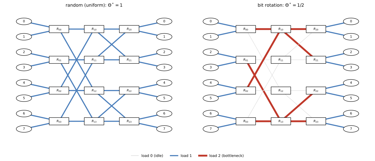
Channel loads on the 8-port butterfly of Figure 16.13. Left: uniform random traffic loads every channel to exactly 1, so the ideal throughput is 1. Right: the bit-rotation permutation routes all eight flows through only \(R_{10}\) and \(R_{13}\), doubling the load on half the internal channels and idling the other half, so the ideal throughput drops to 1/2.
(b) Summing the load definition of Problem 16.2(c) over all channels counts each unit of traffic once per channel traversed, so
\begin{equation*} \sum_{c \in E} \gamma_c = \sum_{s,d} \lambda_{s,d} H_{s,d} \;\ge\; \sum_{s,d} \lambda_{s,d} H^{\min}_{s,d}, \end{equation*}
where \(H_{s,d}\) is the (possibly non-minimal, possibly split) hop count actually used. Since the maximum is at least the average,
\begin{equation*} \gamma_{\max} \;\ge\; \frac{1}{|E|}\sum_{c}\gamma_c \;\ge\; \frac{\sum_{s,d}\lambda_{s,d}H^{\min}_{s,d}}{|E|}, \qquad\text{hence}\qquad \Theta^* \;\le\; \frac{b\,|E|}{\sum_{s,d}\lambda_{s,d}H^{\min}_{s,d}} . \end{equation*}
Here \(|E| = 16\times4 = 64\), and the one-dimensional distances from any node are \(\{0,1,2,1\}\), so the mean hop count over all 16 destinations is \(H^{\min}_{\text{avg}} = 2\).
(i) Random traffic. With \(\lambda_{s,d} = 1/16\), \(\sum_{s,d}\lambda_{s,d}H^{\min}_{s,d} = 16\times2 = 32\), so \(\Theta^* \le 64/32 = 2\), and this is achieved: by vertex- and edge-transitivity, dimension-order routing averaged over the two dimension orders loads every channel at \(\gamma_c = 32/64 = 0.5\). The LP of Problem 16.2(e) returns \(\Theta^* = 2\). (The bisection gives the same converse: 8 channels cross each way and 8 nodes each send \(\Theta/2\) across, so \(4\Theta \le 8\).)
(ii) Bit rotation. The printed pattern is defined only for 3-bit butterfly addresses, so on 16 nodes I read it as \(\pi(a_3a_2a_1a_0) = a_2a_1a_0a_3\) (rotating the other way gives the same value). Its 14 moving flows again total minimal hop count 32, so the counting bound still gives only \(\Theta^* \le 2\), but the LP returns \(\Theta^* = 12/7\), and the cut \(S = \{1,4,5,6,7,9,13\}\) certifies it: \(\pi\) sends all seven nodes of \(S\) outside \(S\) (to \(2,8,10,12,14,3,11\)), a demand of \(7\Theta\) across only 12 outgoing channels, so \(\Theta \le 12/7\). LP flow and cut match, so \(\Theta^* = 12/7\) exactly.
import numpy as np
from fractions import Fraction
from scipy.optimize import linprog
k, N = 4, 16 # 4-ary 2-cube: the 4x4 torus of Figure 16.14
def xy(v): return (v % k, v // k)
def vid(x, y): return (y % k)*k + (x % k)
chans = sorted({(v, w) for v in range(N) for w in
(lambda x, y: (vid(x+1,y), vid(x-1,y), vid(x,y+1), vid(x,y-1)))(*xy(v))})
C = len(chans)
A = np.zeros((N, C))
for c, (t, h) in enumerate(chans):
A[t, c] = 1.0; A[h, c] = -1.0
def hops(u, v):
(a,b), (c_,d_) = xy(u), xy(v)
return min((a-c_) % k, (c_-a) % k) + min((b-d_) % k, (d_-b) % k)
print("nodes = %d, unidirectional channels |E| = %d" % (N, C))
def ideal_throughput(lam, tag):
lam = lam.copy(); np.fill_diagonal(lam, 0.0) # self-traffic uses no channel
F = np.array([[lam[i,d] if i != d else -lam[:,d].sum() for i in range(N)]
for d in range(N)])
nv = N*C + 1
Aeq = np.zeros((N*N, nv))
for d in range(N):
for i in range(N):
Aeq[d*N+i, d*C:(d+1)*C] = A[i]; Aeq[d*N+i, -1] = -F[d, i]
Aub = np.zeros((C, nv))
for c in range(C): Aub[c, [d*C+c for d in range(N)]] = 1.0
obj = np.zeros(nv); obj[-1] = -1.0
r = linprog(obj, A_ub=Aub, b_ub=np.ones(C), A_eq=Aeq, b_eq=np.zeros(N*N), bounds=(0, None))
H = sum(lam[s,d]*hops(s,d) for s in range(N) for d in range(N))
print("%-16s sum_lam*H = %5.2f hop bound |E|/sum_lam*H = %.4f LP Theta* = %.4f"
% (tag, H, C/H, r.x[-1]))
ideal_throughput(np.full((N,N), 1/16.0), "uniform random")
pi = {a: ((a & 7) << 1) | (a >> 3) for a in range(N)} # a3a2a1a0 -> a2a1a0a3
lam_p = np.zeros((N,N))
for a in range(N): lam_p[a, pi[a]] = 1.0
print("bit rotation pi :", pi)
ideal_throughput(lam_p, "bit rotation")
# certificate: search all 2^16 cuts for the tightest cap(S)/demand(S) bound
best = None
for mask in range(1, 2**N - 1):
S = {v for v in range(N) if mask >> v & 1}
T = sum(1 for a in S if pi[a] not in S)
if T == 0: continue
cap = sum(1 for (t, h) in chans if t in S and h not in S)
if best is None or Fraction(cap, T) < best[0]:
best = (Fraction(cap, T), sorted(S), cap, T)
print("tightest cut bound: cap/demand = %s = %.6f, S = %s (cap %d, demand %d)"
% (best[0], float(best[0]), best[1], best[2], best[3]))
nodes = 16, unidirectional channels |E| = 64
uniform random sum_lam*H = 32.00 hop bound |E|/sum_lam*H = 2.0000 LP Theta* = 2.0000
bit rotation pi : {0: 0, 1: 2, 2: 4, 3: 6, 4: 8, 5: 10, 6: 12, 7: 14, 8: 1, 9: 3, 10: 5, 11: 7, 12: 9, 13: 11, 14: 13, 15: 15}
bit rotation sum_lam*H = 32.00 hop bound |E|/sum_lam*H = 2.0000 LP Theta* = 1.7143
tightest cut bound: cap/demand = 12/7 = 1.714286, S = [1, 4, 5, 6, 7, 9, 13] (cap 12, demand 7)
Problem 16.5 — Rearrangably non-blocking Clos networks
Rearrangably non-blocking Clos networks. We have seen how big \(m\) needs to be for a Clos network to be non-blocking. It turns out that \(m\) can be smaller if we ask for a weaker condition of rearrangably non-blocking.
(a) Design an algorithm for routing traffic on an \((m,n,r)\) Clos network with \(m \ge n\).
(b) Consider a \((3,3,4)\) Clos network along with its traffic illustrated in Figure 16.15. In Figure 16.15, each node represents an input/output switch, and links with three different dotted styles represent the middle switches assigned. Figure 16.15 draws four input switches \(I1, I2, I3, I4\) down the left side and four output switches \(O1, O2, O3, O4\) down the right side, with nine connections drawn in three dotted line styles: sessions \((I2,O4)\), \((I3,O1)\), and \((I4,O2)\) are routed through middle switch 1; sessions \((I1,O4)\), \((I2,O1)\), and \((I3,O3)\) are routed through middle switch 2; and sessions \((I1,O2)\), \((I3,O4)\), and \((I4,O1)\) are routed through middle switch 3.
Now, route a new call \((I4,O3)\) using your algorithm from (a). (difficulty: \(\star\star\star\))
(a) Paull’s looping algorithm, below; (b) it routes \((I4,O3)\) through middle switch 2 after recolouring a five-call chain.
A middle-switch assignment is exactly a proper edge colouring, with \(m\) colours, of the bipartite multigraph \(G\) whose vertices are the \(r\) input and \(r\) output switches and whose edges are the active sessions: \(I_a\) has one link per middle switch, so no two edges at \(I_a\) may share a colour, and likewise at \(O_b\). Each switch has \(n\) ports, so \(\Delta(G) \le n\), and König’s edge-colouring theorem makes \(G\) properly \(\Delta\)-edge-colourable; hence \(m \ge n\) carries any admissible permutation (Slepian-Duguid), against \(m \ge 2n-1\) for strict non-blocking in Section 16.2.1. (The chapter writes \((n,m,r)\) and the problem \((m,n,r)\); in the \((3,3,4)\) instance \(n = m = 3\), so nothing turns on the order.)
(a) In batch, any bipartite edge-colouring routine serves. Online, to add \((I_a,O_b)\) to a valid assignment \(A\):
- Let \(\mathcal{A}\), \(\mathcal{B}\) be the middle switches unused at \(I_a\), \(O_b\). Since each carries at most \(n-1\) other calls and \(m \ge n\), both are nonempty.
- If \(\mathcal{A} \cap \mathcal{B} \ne \emptyset\), route through any common middle switch; no call moves.
- Otherwise pick \(x \in \mathcal{A}\), \(y \in \mathcal{B}\) (so \(x \ne y\)) and walk the alternating chain in the subgraph \(G_{xy}\) of \(x\)- and \(y\)-coloured calls, starting with the \(x\)-edge at \(O_b\).
- Swap \(x \leftrightarrow y\) along that chain and route \((I_a,O_b)\) through \(x\).
Correctness: every vertex of \(G_{xy}\) has degree at most 2, so components are paths and even cycles, and swapping colours along one whole component keeps \(A\) proper while touching nothing outside it. The chain from \(O_b\) is a path, since \(O_b\) has no \(y\)-edge, so after the swap its chain edge is \(y\) and \(x\) is free at \(O_b\). The chain cannot reach \(I_a\), because every input-switch vertex on it is entered by an \(x\)-edge while \(x \in \mathcal{A}\) means \(I_a\) has none; so \(x\) is free at both ends and step 4 succeeds, moving at most \(2r-1\) calls.
(b) Current state, per switch:
- \(I1\): \(O4 \to 2\), \(O2 \to 3\). Free at \(I1\): \(\{1\}\).
- \(I2\): \(O4 \to 1\), \(O1 \to 2\). Free at \(I2\): \(\{3\}\).
- \(I3\): \(O1 \to 1\), \(O3 \to 2\), \(O4 \to 3\). Full.
- \(I4\): \(O2 \to 1\), \(O1 \to 3\). Free at \(I4\): \(\{2\}\).
- \(O3\): \(I3 \to 2\). Free at \(O3\): \(\{1,3\}\).
Here \(\mathcal{A} = \{2\}\) and \(\mathcal{B} = \{1,3\}\) are disjoint, so a rearrangement is forced. Take \(x = 2\), \(y = 1\); \(G_{21}\) has \(x\)-edges \((I1,O4), (I2,O1), (I3,O3)\) and \(y\)-edges \((I2,O4), (I3,O1), (I4,O2)\), and walking from \(O3\),
\begin{equation*} O3 \;\xrightarrow{\,2\,}\; I3 \;\xrightarrow{\,1\,}\; O1 \;\xrightarrow{\,2\,}\; I2 \;\xrightarrow{\,1\,}\; O4 \;\xrightarrow{\,2\,}\; I1, \end{equation*}
the chain stops at \(I1\), which has no middle-1 call, and as predicted omits \(I4\). Swapping colours along it,
\begin{equation*} (I3,O3): 2 \to 1, \quad (I3,O1): 1 \to 2, \quad (I2,O1): 2 \to 1, \quad (I2,O4): 1 \to 2, \quad (I1,O4): 2 \to 1, \end{equation*}
which frees middle switch 2 at \(O3\), so \((I4,O3)\) routes through middle switch 2. The assignment, with five of the nine old calls moved, is
- middle 1: \((I1,O4)\), \((I2,O1)\), \((I3,O3)\), \((I4,O2)\)
- middle 2: \((I2,O4)\), \((I3,O1)\), \((I4,O3)\)
- middle 3: \((I1,O2)\), \((I3,O4)\), \((I4,O1)\)
and every switch now sees distinct middle switches (Check!); middle 1 carrying four sessions is admissible since a middle switch is \(r \times r = 4\times4\).
n, m, r = 3, 3, 4 # (n,m,r) Clos of Figure 16.15: 4 in/out switches, 3 middles
# existing assignment: session (input switch, output switch) -> middle switch
assign = {(2,4):1, (3,1):1, (4,2):1,
(1,4):2, (2,1):2, (3,3):2,
(1,2):3, (3,4):3, (4,1):3}
def valid(A):
for a in range(1, r+1):
ks = [k for (i,o),k in A.items() if i == a]
if len(ks) != len(set(ks)): return False
for b in range(1, r+1):
ks = [k for (i,o),k in A.items() if o == b]
if len(ks) != len(set(ks)): return False
return True
def route(A, a, b):
A = dict(A)
free_a = set(range(1,m+1)) - {k for (i,o),k in A.items() if i == a}
free_b = set(range(1,m+1)) - {k for (i,o),k in A.items() if o == b}
print("free middles at I%d: %s ; free at O%d: %s ; intersection: %s"
% (a, sorted(free_a), b, sorted(free_b), sorted(free_a & free_b)))
if free_a & free_b:
x = min(free_a & free_b); A[(a,b)] = x
print("no rearrangement needed: route (I%d,O%d) via middle %d" % (a,b,x))
return A
x, y = min(free_a), min(free_b)
print("pick x = %d (free at I%d), y = %d (free at O%d); build alternating chain from O%d"
% (x, a, y, b, b))
chain, seen = [], set()
node, colour, side = b, x, 'out'
while True:
cand = [e for e,k in A.items() if k == colour and e not in seen
and (e[1] == node if side == 'out' else e[0] == node)]
if not cand: break
e = cand[0]; chain.append((e, colour)); seen.add(e)
node, colour, side = ((e[0], y if colour == x else x, 'in') if side == 'out'
else (e[1], y if colour == x else x, 'out'))
for (i,o), old in chain:
new = y if old == x else x
print(" recolour (I%d,O%d): middle %d -> %d" % (i, o, old, new))
A[(i,o)] = new
A[(a,b)] = x
print("middle %d is now free at O%d -> route (I%d,O%d) through middle %d" % (x, b, a, b, x))
return A
print("initial assignment valid:", valid(assign))
new = route(assign, 4, 3)
print()
print("final assignment (input switch -> {output switch: middle}):")
for a in range(1, r+1):
print(" I%d: %s" % (a, {"O%d" % o: k for (i,o),k in sorted(new.items()) if i == a}))
print("valid Clos routing:", valid(new))
for k in range(1, m+1):
print(" middle %d carries: %s" % (k, sorted("(I%d,O%d)" % e for e,v in new.items() if v == k)))
initial assignment valid: True
free middles at I4: [2] ; free at O3: [1, 3] ; intersection: []
pick x = 2 (free at I4), y = 1 (free at O3); build alternating chain from O3
recolour (I3,O3): middle 2 -> 1
recolour (I3,O1): middle 1 -> 2
recolour (I2,O1): middle 2 -> 1
recolour (I2,O4): middle 1 -> 2
recolour (I1,O4): middle 2 -> 1
middle 2 is now free at O3 -> route (I4,O3) through middle 2
final assignment (input switch -> {output switch: middle}):
I1: {'O2': 3, 'O4': 1}
I2: {'O1': 1, 'O4': 2}
I3: {'O1': 2, 'O3': 1, 'O4': 3}
I4: {'O1': 3, 'O2': 1, 'O3': 2}
valid Clos routing: True
middle 1 carries: ['(I1,O4)', '(I2,O1)', '(I3,O3)', '(I4,O2)']
middle 2 carries: ['(I2,O4)', '(I3,O1)', '(I4,O3)']
middle 3 carries: ['(I1,O2)', '(I3,O4)', '(I4,O1)']
IPTV and Netflix: How can the Internet support video?
Problem 17.1 — Video-viewing models
Video-viewing models. Fill in the table indicating which video-watching models are infeasible. Provide examples of companies that follow each feasible model. Some rows have been filled out as an example.
The table has four classification columns – real-time or precoded, streaming or download, channelized or on-demand, unicast or multicast – plus a companies column, and enumerates all \(2^4 = 16\) combinations in the following order:
| Real-time or precoded | Streaming or download | Channelized or on-demand | Unicast or multicast | Companies |
|---|---|---|---|---|
| Real-time | Streaming | Channelized | Unicast | |
| Real-time | Streaming | Channelized | Multicast | |
| Real-time | Streaming | On-demand | Unicast | |
| Real-time | Streaming | On-demand | Multicast | |
| Real-time | Download | Channelized | Unicast | |
| Real-time | Download | Channelized | Multicast | |
| Real-time | Download | On-demand | Unicast | |
| Real-time | Download | On-demand | Multicast | |
| Precoded | Streaming | Channelized | Unicast | |
| Precoded | Streaming | Channelized | Multicast | |
| Precoded | Streaming | On-demand | Unicast | YouTube, Hulu, NBC, HBO Go |
| Precoded | Streaming | On-demand | Multicast | Infeasible (on-demand multicast) |
| Precoded | Download | Channelized | Unicast | |
| Precoded | Download | Channelized | Multicast | |
| Precoded | Download | On-demand | Unicast | |
| Precoded | Download | On-demand | Multicast |
(difficulty: \(\star\))
Nine of the 16 combinations are feasible; the seven infeasible ones follow from the two exclusion rules of Section 17.1.1.
Rule 1: real-time implies streaming, since download playback begins only after the file (or a large prefix) has landed, and real-time content does not yet exist then – this kills the four (Real-time, Download) rows. Rule 2: true VoD cannot be multicast, since multicast amortises one transmission over viewers consuming the same bits at the same instant and on-demand start times destroy that synchronisation – this kills the four (On-demand, Multicast) rows. The rules overlap in one row, so \(4 + 4 - 1 = 7\) are infeasible.
| Real-time / precoded | Streaming / download | Channelized / on-demand | Unicast / multicast | Companies / verdict |
|---|---|---|---|---|
| Real-time | Streaming | Channelized | Unicast | Twitch, Ustream, Sling TV, Slingbox: one live channel, one TCP/UDP flow per viewer |
| Real-time | Streaming | Channelized | Multicast | Classic IPTV live channels: AT&T U-verse, Verizon FiOS TV; also broadcast and DirecTV |
| Real-time | Streaming | On-demand | Unicast | Skype, FaceTime, Google Hangouts, WebEx: the live stream is generated on request |
| Real-time | Streaming | On-demand | Multicast | Infeasible (on-demand multicast, Rule 2) |
| Real-time | Download | Channelized | Unicast | Infeasible (real-time cannot be downloaded, Rule 1) |
| Real-time | Download | Channelized | Multicast | Infeasible (Rule 1) |
| Real-time | Download | On-demand | Unicast | Infeasible (Rule 1) |
| Real-time | Download | On-demand | Multicast | Infeasible (Rules 1 and 2 both) |
| Precoded | Streaming | Channelized | Unicast | Pandora and internet-radio-style linear channels; NVoD delivered per-viewer; Pluto TV |
| Precoded | Streaming | Channelized | Multicast | Most IPTV movie and re-run channels (HBO, Comcast linear); NVoD staggered multicast |
| Precoded | Streaming | On-demand | Unicast | YouTube, Hulu, NBC, HBO Go (given) |
| Precoded | Streaming | On-demand | Multicast | Infeasible (on-demand multicast) (given) |
| Precoded | Download | Channelized | Unicast | Podcast subscriptions, iTunes Season Pass, TiVo/DVR scheduled recording |
| Precoded | Download | Channelized | Multicast | Overnight push-VoD pre-positioning into set-top boxes: Sky Anytime, DirecTV datacast |
| Precoded | Download | On-demand | Unicast | iTunes movie purchase/rental, Amazon Instant Video download, Google Play movies |
| Precoded | Download | On-demand | Multicast | Infeasible (on-demand multicast, Rule 2) |
Three entries are easily misclassified. Real-time plus on-demand is consistent, since “on-demand” fixes who chooses the start time, not whether the content pre-exists: a video call qualifies. Precoded, download, channelized multicast is the overnight push-VoD carousel, which dodges Rule 2 by multicasting the file on a schedule and letting the viewer be on-demand against local storage. And a P2P swarm (BitTorrent, PPLive of Section 17.1.2) is not on-demand multicast: each peer receives separately-scheduled unicast piece transfers, so the last row stays infeasible.
Problem 17.2 — Compression–reliability tradeoff
Compression–reliability tradeoff. Let us examine the tradeoff between compression and error resilience through a back-of-the-envelope calculation. Suppose we have 15 frames to transmit and two possible GoP structures: (1) IPB and (2) IPBBB. Suppose an I frame costs 7 kB, a P frame costs 3 kB, and a B frame costs 1 kB.
If an entire GoP is not received correctly, we assume that the GoP must be sent again. As our metric of error resilience, consider the expected number of bits that must be retransmitted at least once. The probability of dropping a frame is 1% and assumed to be independent. (These assumptions are made to simplify this homework problem. In a realistic setting, if a P or B frame in a GoP is lost, the entire GoP does not need to be retransmitted. Loss is not independent and usually much less than 1%. And there should be many more frames in a video clip.)
(a) In case 1, the video frame structure is IPB/IPB/IPB/IPB/IPB. What is the total cost of the video in kB? What is the cost per GoP per kB?
(b) What is the probability that an entire GoP is transmitted successfully in case 1? What is the expected number of GoPs that are successful on the first attempt at the transmission of the entire video? What is the expected number of GoPs that must be retransmitted at least once? How much does the first retransmission cost in kB?
(c) Repeat (a) for case 2, where the video frame structure is now: IPBBB/IPBBB/IPBBB.
(d) Repeat (b) for case 2.
(e) Compare your results from (a), (b), (c), and (d) in terms of the tradeoff of compressibility vs. retransmission. What can you conclude?
(difficulty: \(\star\))
Case 1 costs 55 kB with 1.634 kB of first retransmission; case 2 costs 39 kB with 1.911 kB, so the longer GoP wins at this loss rate.
(a) Fifteen frames in threes is \(N_1 = 5\) GoPs at \(c_1 = 7+3+1 = 11\) kB, so 55 kB total, i.e. \(55/15 = 3.67\) kB per frame.
(b) Frames survive independently with probability \(0.99\), so with \(s_1 = 0.99^3 = 0.970299\) the count intact on the first attempt is Binomial\((5, s_1)\) and
\begin{align*} 5 s_1 &= 4.851495, & 5(1-s_1) &= 0.148505 \text{ GoPs},\\ && 0.148505 \times 11 &= 1.634 \text{ kB}, \end{align*}
the last being the first retransmission round (whole GoPs resent), \(2.97\%\) of 55 kB.
(c) Fifteen frames in fives is \(N_2 = 3\) GoPs at \(c_2 = 7+3+1+1+1 = 13\) kB, so 39 kB, i.e. 2.6 kB per frame – \(29.1\%\) cheaper, since four B frames (4 kB) displace two I and two P frames (20 kB).
(d) With \(s_2 = 0.99^5 = 0.950990\),
\begin{align*} 3 s_2 &= 2.852970, & 3(1-s_2) &= 0.147030 \text{ GoPs},\\ && 0.147030 \times 13 &= 1.911 \text{ kB}, \end{align*}
the retransmission round now being \(4.90\%\) of 39 kB.
from scipy.optimize import brentq
p = 0.01
q = 1 - p
def case(name, frames_per_gop, cost_per_gop, n_gop):
total = n_gop * cost_per_gop
ps = q ** frames_per_gop
print(name)
print(f" cost per GoP = {cost_per_gop} kB")
print(f" total video cost = {total} kB")
print(f" P(GoP arrives intact) = {ps:.6f}")
print(f" E[GoPs ok on first try] = {n_gop*ps:.6f}")
print(f" E[GoPs retransmitted] = {n_gop*(1-ps):.6f}")
print(f" first retransmission = {n_gop*(1-ps)*cost_per_gop:.6f} kB")
print(f" retx / original = {100*n_gop*(1-ps)*cost_per_gop/total:.3f} %")
print(f" E[bytes until success] = {total/ps:.4f} kB")
case("case 1 IPB (5 GoPs)", 3, 7+3+1, 5)
case("case 2 IPBBB (3 GoPs)", 5, 7+3+1+1+1, 3)
print(f"case 2 saves {100*(1-39/55):.2f} % of the bits")
print(f"case 2 costs {100*(1.911388/1.633555-1):.2f} % more first-retransmission bits")
crossover = brentq(lambda x: 5*11/(1-x)**3 - 3*13/(1-x)**5, 1e-9, 0.9)
print(f"loss rate at which case 1 finally wins: p = {crossover:.4f}")
case 1 IPB (5 GoPs)
cost per GoP = 11 kB
total video cost = 55 kB
P(GoP arrives intact) = 0.970299
E[GoPs ok on first try] = 4.851495
E[GoPs retransmitted] = 0.148505
first retransmission = 1.633555 kB
retx / original = 2.970 %
E[bytes until success] = 56.6836 kB
case 2 IPBBB (3 GoPs)
cost per GoP = 13 kB
total video cost = 39 kB
P(GoP arrives intact) = 0.950990
E[GoPs ok on first try] = 2.852970
E[GoPs retransmitted] = 0.147030
first retransmission = 1.911388 kB
retx / original = 4.901 %
E[bytes until success] = 41.0099 kB
case 2 saves 29.09 % of the bits
case 2 costs 17.01 % more first-retransmission bits
loss rate at which case 1 finally wins: p = 0.1579
(e) Lengthening the GoP buys \(29.1\%\) of the bits and costs \(17.0\%\) of the far smaller retransmission volume, the asymmetry being structural: the saving scales with the frame budget, while the penalty carries a factor \(1-(1-p)^n \approx np\). Charging geometric retries at \(c/s\) expected bits per GoP,
\begin{equation*} \text{case 1: } \frac{5 \times 11}{0.99^3} = 56.68 \text{ kB}, \qquad \text{case 2: } \frac{3 \times 13}{0.99^5} = 41.01 \text{ kB}, \end{equation*}
so case 2 wins by 28%, and equating the two gives the crossover
\begin{equation*} (1-p)^2 = \tfrac{39}{55} \iff p = 1 - \sqrt{39/55} = 0.1579 . \end{equation*}
The short GoP only wins once about 16% of frames drop, far above real IP video paths; at realistic loss rates compression efficiency dominates, and the binding limit on GoP length is instead the instant-channel-change delay of Section 17.2.1.
Problem 17.3 — Playback buffer with random arrival time
Playback buffer with random arrival time. We will look at a question similar to the example in Section 17.3.2 examining the latency–jitter tradeoff, but with a probabilistic packet arrival time. Suppose \(V_1 = 0\), \(V_2 = 1\), and \(V_3 = 2\), i.e., a step function. Now the packets arrive independently at times \(A_1\), \(A_2\), and \(A_3\), where \(A_i\) is drawn randomly between \(\bar{A}_i - 1\) and \(\bar{A}_i + 1\), and we set \(\bar{A}_1 = 3\), \(\bar{A}_2 = 4.2\), \(\bar{A}_3 = 4.6\). What is the optimal playback time of the first packet \(p^*\) that minimizes latency but ensures that all packets are received with at least a 95% probability?
(difficulty: \(\star\star\))
\(p^* = 4.1\) s, with \(P_2^* = 5.1\) and \(P_3^* = 6.1\); packet 2 alone binds.
The constraint \(P_{i+1} = P_i + 1\) of Section 17.3.2 makes P a unit step, so \(P_i = p + (i-1)\) and, both curves being unit steps, minimising \(\sum_i(P_i - V_i)\) is minimising \(p\). Only the arrival constraint changes: it becomes the joint chance constraint
\begin{equation*} \min_{p} \; p \quad \text{s.t.} \quad \Pr\!\left[\bigcap_{i=1}^{3}\{A_i \le p + i - 1\}\right] \ge 0.95 . \end{equation*}
Each \(A_i \sim \mathrm{Uniform}(\bar{A}_i - 1, \bar{A}_i + 1)\) has CDF \(F_i(x) = \operatorname{clip}((x - \bar{A}_i + 1)/2, 0, 1)\), and independence factorises the constraint into \(\Pi(p) = \prod_i F_i(p + i - 1)\), i.e. (before clipping)
\begin{equation*} F_1(p) = \frac{p-2}{2}, \qquad F_2(p+1) = \frac{p-2.2}{2}, \qquad F_3(p+2) = \frac{p-1.6}{2}. \end{equation*}
A product of factors in \([0,1]\) is at most its smallest, so \(\Pi(p) \ge 0.95\) forces every factor to \(0.95\); factors 1 and 3 saturate at \(p = 4\) and \(p = 3.6\) while factor 2 needs \(p \ge 4.1\), so packet 2 binds and
\begin{equation*} \Pi(4.1) = 1 \times 0.95 \times 1 = 0.95 . \end{equation*}
Since \(\Pi\) is nondecreasing and \(\Pi(p) < 0.95\) for \(p < 4.1\), \(p^* = 4.1\) s.
import numpy as np
import matplotlib.pyplot as plt
Abar = np.array([3.0, 4.2, 4.6])
V = np.array([0.0, 1.0, 2.0])
def psucc(p):
p = np.asarray(p, dtype=float)
out = np.ones_like(p)
for i in range(3):
out = out * np.clip((p + i - (Abar[i] - 1)) / 2.0, 0.0, 1.0)
return out
grid = np.linspace(2.0, 5.4, 3401)
pstar = grid[np.argmax(psucc(grid) >= 0.95)]
print(f"grid search p* = {pstar:.4f}")
print(f"closed form p* = 4.1, P = {float(psucc(4.1)):.6f}")
for p in [3.2, 3.6, 4.0, 4.05, 4.1, 4.2]:
print(f" p = {p:.2f} P(all packets in time) = {float(psucc(p)):.4f}")
rng = np.random.default_rng(0)
N = 2_000_000
A = rng.uniform(Abar - 1, Abar + 1, size=(N, 3))
for p in [4.0, 4.1]:
ok = np.all(A <= p + np.arange(3), axis=1).mean()
print(f"Monte Carlo (2e6 draws) p = {p}: {ok:.5f}")
d = Abar - V
print(f"deterministic case: d = {d}, D = {d.max()-d[0]:.1f}, p = {Abar[0]+d.max()-d[0]:.1f}")
fig, ax = plt.subplots(figsize=(7, 4.2))
ax.plot(grid, psucc(grid), lw=2, color='#1f5f9e')
ax.axhline(0.95, ls='--', color='0.4')
ax.axvline(4.1, ls=':', color='crimson')
ax.plot([4.1], [0.95], 'o', color='crimson')
ax.annotate(r'$p^*=4.1$', (4.1, 0.95), textcoords='offset points', xytext=(10, -22))
ax.axvline(3.2, ls=':', color='green')
ax.annotate('deterministic\nanswer 3.2', (3.2, 0.35),
textcoords='offset points', xytext=(6, 0), color='green')
ax.set_xlabel('playback time of first packet $p$ (s)')
ax.set_ylabel('P(no packet misses its deadline)')
ax.set_ylim(-0.02, 1.05)
ax.grid(alpha=0.3)
plt.savefig('nl-ch17-playback-success.svg', dpi=150, bbox_inches='tight')
grid search p* = 4.1010
closed form p* = 4.1, P = 0.950000
p = 3.20 P(all packets in time) = 0.2400
p = 3.60 P(all packets in time) = 0.5600
p = 4.00 P(all packets in time) = 0.9000
p = 4.05 P(all packets in time) = 0.9250
p = 4.10 P(all packets in time) = 0.9500
p = 4.20 P(all packets in time) = 1.0000
Monte Carlo (2e6 draws) p = 4.0: 0.90004
Monte Carlo (2e6 draws) p = 4.1: 0.95000
deterministic case: d = [3. 3.2 2.6], D = 0.2, p = 3.2
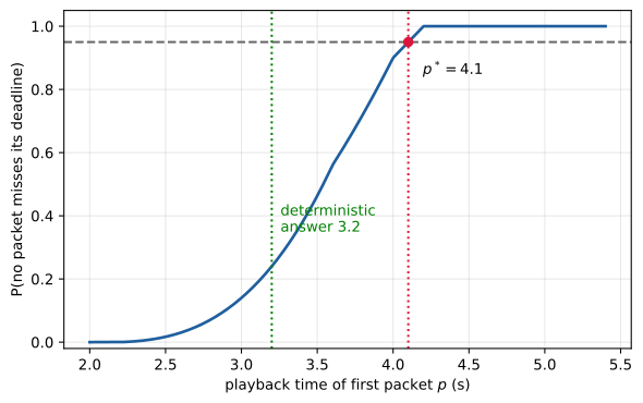
Probability that no packet misses its playback deadline, as a function of the first packet’s playback time \(p\). The curve is the product of three clipped uniform CDFs; it crosses the 95% line at \(p^* = 4.1\) s and saturates at 1 at \(p = 4.2\) s. The deterministic answer from Section 17.3.2’s formula, \(p = 3.2\) s, buys only a 24% chance of glitch-free playback.
By contrast, Section 17.3.2’s deterministic formula \(P_1^* = A_1 + D\) with \(D = \max_i(d_i - d_1)\) applied to the means gives \(d = \bar{A} - V = (3, 3.2, 2.6)\), so \(D = 0.2\) and \(P_1^* = 3.2\) s – a schedule the code shows succeeds only \(24\%\) of the time. The extra \(0.9\) s is paying for the \(\pm 1\) s jitter support rather than for the \(0.2\) s spread of the means.
Problem 17.4 — Round robin, weighted fair queueing, and priority queueing
Round robin, weighted fair queueing, and priority queueing. We compare three resource allocation policies. Recall the following.
- Round robin simply gives each queue a turn to transmit a packet.
- Priority queueing allows the queue with the higher priority to be continuously serviced until it is empty.
- A particular implementation of weighted fair queueing looks at the head of each queue and transmits the packet that would finish transmission quickest under the Generalized Processor Sharing (GPS) scheme. GPS is an ideal “fluid-flow” scheduler, and is defined as follows: if we have \(n\) queues with priority \(p_1, p_2, \ldots, p_n\), then the bandwidth allocated to queue \(j\) per timeslot is \(p_j / \sum_i p_i\).
Suppose we have queue A and queue B with packets arriving as follows. At \(t = 0\) a packet of size 3 arrives at queue B. At \(t = 1\) a packet of size 1 arrives at queue A. At \(t = 2\) a packet of size 1 arrives at queue A. At \(t = 3\) a packet of size 2 arrives at queue B. Nothing arrives at \(t = 4\). At \(t = 5\) a packet of size 4 arrives at queue B.
Queue A has priority 1 and Queue B has priority 3 (higher number indicating higher priority). The outgoing link has bandwidth 1 Mbps. Once a packet has begun transmitting, it cannot be pre-empted by other packets. Fill in a table of departed packet sizes for queue A and queue B at each of \(t = 0, 1, 2, 3, 4, 5\), for round-robin scheduling, priority queueing, and weighted fair queueing.
(difficulty: \(\star\star\))
RR and WFQ produce the same schedule here; PQ starves A. Sizes are megabits on a 1 Mbps link, so a size-\(L\) packet holds the link for \(L\) seconds and, all three disciplines being work-conserving (Section 17.4.1), decisions are made only when the link goes idle.
(i) Round robin. Only B is backlogged at \(t = 0\), so B(3) occupies \([0,3)\); A’s turn then gives A(1) in \([3,4)\); B’s size-2 packet (arrived \(t=3\)) takes \([4,6)\).
(ii) Priority queueing. B outranks A and stays backlogged throughout: B(3) in \([0,3)\), B(2) in \([3,5)\) since it arrives exactly at \(t=3\), then B(4) in \([5,9)\), so A departs nothing before \(t = 10\).
(iii) WFQ. With \(p_A = 1\), \(p_B = 3\), GPS gives a backlogged A \(1/4\) Mbps against B’s \(3/4\), and the whole 1 Mbps to a lone backlogged class. So B(3) drains at rate 1 on \([0,1)\) and at \(3/4\) on \([1,3)\), leaving \(0.5\) Mb and \(G = 3 + 2/3 = 3.667\), while A(1) drains at \(1/4\) on \([1,3)\), leaving \(0.5\) Mb and \(G = 5\). Then B(2) runs from \(3.667\) at \(3/4\) to \(G = 6.333\), A’s second packet from \(5\) at \(1/4\) to \(G = 9\), and B(4) from \(6.333\) at \(3/4\) until A empties at \(t=9\) and then at rate 1, to \(G = 11\). The order B(3), A(1), B(2), A(1), B(4) is exactly round robin’s.
C = 1.0
prio = {'A': 1.0, 'B': 3.0}
arrivals = [(0.0, 'B', 3.0), (1.0, 'A', 1.0), (2.0, 'A', 1.0),
(3.0, 'B', 2.0), (5.0, 'B', 4.0)]
def gps_finish_times(arrivals):
q = {}
for j, (t, c, L) in enumerate(sorted(arrivals)):
q.setdefault(c, []).append([t, L, j])
head = {c: 0 for c in q}
G, now = {}, 0.0
while any(head[c] < len(q[c]) for c in q):
act = [c for c in q if head[c] < len(q[c]) and q[c][head[c]][0] <= now + 1e-12]
fut = [q[c][head[c]][0] for c in q
if head[c] < len(q[c]) and q[c][head[c]][0] > now + 1e-12]
if not act:
now = min(fut)
continue
tot = sum(prio[c] for c in act)
rate = {c: prio[c] / tot * C for c in act}
tfin, cfin = min((now + q[c][head[c]][1] / rate[c], c) for c in act)
tnext = min([tfin] + fut)
for c in act:
q[c][head[c]][1] -= rate[c] * (tnext - now)
now = tnext
if abs(tnext - tfin) < 1e-12:
G[q[cfin][head[cfin]][2]] = now
head[cfin] += 1
return G
G = gps_finish_times(arrivals)
srt = sorted(arrivals)
print("GPS fluid finish times (the WFQ service order):")
for j in sorted(G, key=lambda j: G[j]):
t, c, L = srt[j]
print(f" class {c}, size {L:.0f}, arrived t={t:.0f}: G = {G[j]:.4f}")
def run(policy):
pend = sorted(arrivals)
q, i, now, last, log = {'A': [], 'B': []}, 0, 0.0, 'A', []
while True:
while i < len(pend) and pend[i][0] <= now + 1e-12:
t, c, L = pend[i]
q[c].append((t, c, L, i))
i += 1
avail = [c for c in 'AB' if q[c]]
if not avail:
if i >= len(pend):
return log
now = pend[i][0]
continue
if policy == 'RR':
order = ['B', 'A'] if last == 'A' else ['A', 'B']
c = next(cc for cc in order if q[cc])
elif policy == 'PQ':
c = max(avail, key=lambda cc: prio[cc])
else:
c = min(avail, key=lambda cc: G[q[cc][0][3]])
t, cc, L, _ = q[c].pop(0)
log.append((now, now + L / C, c, L, t))
last, now = c, now + L / C
for pol in ['RR', 'PQ', 'WFQ']:
log = run(pol)
print(f"=== {pol} ===")
print(" departure table, t = 0..5")
print(" t | A departs | B departs")
for t in range(6):
row = {'A': '-', 'B': '-'}
for s, f, c, L, a in log:
if abs(f - t) < 1e-9:
row[c] = f"{L:.0f}"
print(f" {t} | {row['A']:>3} | {row['B']:>3}")
print(" full timeline beyond t=5:")
for s, f, c, L, a in log:
print(f" {c} size {L:.0f} arr t={a:.0f} served [{s:.0f},{f:.0f}) "
f"departs t={f:.0f} delay {f-a:.0f}")
dA = [f - a for s, f, c, L, a in log if c == 'A']
dB = [f - a for s, f, c, L, a in log if c == 'B']
print(f" mean delay: A = {sum(dA)/len(dA):.2f} B = {sum(dB)/len(dB):.2f} "
f"overall = {(sum(dA)+sum(dB))/5:.2f}")
GPS fluid finish times (the WFQ service order):
class B, size 3, arrived t=0: G = 3.6667
class A, size 1, arrived t=1: G = 5.0000
class B, size 2, arrived t=3: G = 6.3333
class A, size 1, arrived t=2: G = 9.0000
class B, size 4, arrived t=5: G = 11.0000
=== RR ===
departure table, t = 0..5
t | A departs | B departs
0 | - | -
1 | - | -
2 | - | -
3 | - | 3
4 | 1 | -
5 | - | -
full timeline beyond t=5:
B size 3 arr t=0 served [0,3) departs t=3 delay 3
A size 1 arr t=1 served [3,4) departs t=4 delay 3
B size 2 arr t=3 served [4,6) departs t=6 delay 3
A size 1 arr t=2 served [6,7) departs t=7 delay 5
B size 4 arr t=5 served [7,11) departs t=11 delay 6
mean delay: A = 4.00 B = 4.00 overall = 4.00
=== PQ ===
departure table, t = 0..5
t | A departs | B departs
0 | - | -
1 | - | -
2 | - | -
3 | - | 3
4 | - | -
5 | - | 2
full timeline beyond t=5:
B size 3 arr t=0 served [0,3) departs t=3 delay 3
B size 2 arr t=3 served [3,5) departs t=5 delay 2
B size 4 arr t=5 served [5,9) departs t=9 delay 4
A size 1 arr t=1 served [9,10) departs t=10 delay 9
A size 1 arr t=2 served [10,11) departs t=11 delay 9
mean delay: A = 9.00 B = 3.00 overall = 5.40
=== WFQ ===
departure table, t = 0..5
t | A departs | B departs
0 | - | -
1 | - | -
2 | - | -
3 | - | 3
4 | 1 | -
5 | - | -
full timeline beyond t=5:
B size 3 arr t=0 served [0,3) departs t=3 delay 3
A size 1 arr t=1 served [3,4) departs t=4 delay 3
B size 2 arr t=3 served [4,6) departs t=6 delay 3
A size 1 arr t=2 served [6,7) departs t=7 delay 5
B size 4 arr t=5 served [7,11) departs t=11 delay 6
mean delay: A = 4.00 B = 4.00 overall = 4.00
The filled tables, entries being the sizes of packets completing at that instant:
| Time (s) | RR: A departs | RR: B departs | PQ: A departs | PQ: B departs | WFQ: A departs | WFQ: B departs |
|---|---|---|---|---|---|---|
| \(t=0\) | – | – | – | – | – | – |
| \(t=1\) | – | – | – | – | – | – |
| \(t=2\) | – | – | – | – | – | – |
| \(t=3\) | – | 3 | – | 3 | – | 3 |
| \(t=4\) | 1 | – | – | – | 1 | – |
| \(t=5\) | – | – | – | 2 | – | – |
Past the table, RR and WFQ deliver B(2) at \(t=6\), A at \(t=7\) and B(4) at \(t=11\); PQ delivers B(4) at \(t=9\) and A’s packets only at \(t=10\) and \(t=11\), for mean delays \(A = 9\), \(B = 3\) against \(4\) and \(4\). All three drain the same 11 Mb by \(t=11\), since all are work-conserving; only the allocation of delay differs.
Two points on the coincidence. WFQ matches RR only because B’s weight shifts the GPS finish times without reordering them – when B(2) becomes eligible at \(t=3\) an A packet already has the smaller finish time. And the answer is robust to the reading of GPS: taking the problem’s non-work-conserving share \(p_j/\sum_i p_i\) instead gives \(G = 4, 5, 6.67, 9, 12\), different numbers in the same order, hence the same schedule.
Problem 17.5 — Leaky bucket and GPS
Leaky bucket and GPS. A link becomes congested when packets arrive at a faster rate than the link can support. The leaky bucket queueing system is one way to solve this problem. There is a bucket that contains tokens. For traffic class \(k\), the bucket has size \(B_k\) and tokens refill the bucket at a rate \(a_k\). Packets wait in the queue and can be released only with a token from the bucket. Therefore, the maximum number of packets that leave the queue during time interval \([u, t]\) is \(B_k + a_k(t - u)\). This is illustrated in Figure 17.11 (a bucket filling with tokens at rate \(a\) up to a maximum of \(B\), feeding a gate that releases a queued packet only when a token is available).
Several leaky buckets drain into the same buffer. This buffer follows the Generalized Processor Sharing (GPS) service. Each traffic class \(k\) has weight \(w_k\); \(C\) bps is the rate supported by the link out of the buffer; and \(\rho_k = \frac{w_k}{\sum_j w_j} C\) is the instantaneous rate at which packets of traffic class \(k\) leave the GPS buffer. This is illustrated in Figure 17.12 (several per-class leaky-bucket-regulated queues all feeding one shared GPS buffer served by a single output link).
(a) During the time interval \([u, t]\), at least \(\rho_k(t-u)\) packets leave the GPS buffer. Let \(B_{t,k}\) be the backlog of traffic class \(k\) in the GPS buffer at time \(t\). Prove that the backlog of class-\(k\) traffic in the buffer cannot exceed some \(B_k\) if \(\rho_k \ge a_k\). To start, assume that there is a time \(t\) when the backlog \(B_{t,k} \ge B_k\). Consider the largest time \(u < t\) such that \(B_{u,k} = 0\), and write the inequality relating the change in backlog size from time \(u\) to time \(t\).
(b) Prove that the delay experienced by a packet in class \(k\) in Figure 17.12 cannot exceed \(\frac{B_k}{\rho_k}\) if \(\rho_k \ge a_k\).
Let \(F_k\) denote the transmission time of packet \(k\) (the time when packet \(k\) leaves the buffer) under WFQ. Similarly define \(G_k\) for GPS. Let \(L_k\) denote the size (in bits) of packet \(k\), and \(L_{max}\) is the largest \(L_k\). We will show that \[ F_k \le G_k + \frac{L_{max}}{C}, \quad \forall k. \qquad (17.1) \] GPS and WFQ both process packets at the same rate, so the total amount of packets in the system remains the same. Therefore, their busy and idle periods are the same, and we need only show that the result holds for a single busy period. Assume \(F_1 < F_2 < \ldots < F_K\) correspond to \(K\) packets in one busy period of WFQ.
(c) Pick any \(k \in \{1, 2, \ldots, K\}\) and find the maximum \(m < k\) such that \(G_m > G_k\). (If there is no such \(m\), let \(m = 0\).) This implies that \(G_n \le G_k < G_m\) for \(n\) in the set of indices \(P = \{m+1, m+2, \ldots, k-1\}\). Let \(T_m\) denote the time when WFQ chose to transmit packet \(m\). Now consider the time \(S_m = F_m - T_m\). Show that the packets in set \(P\) must have arrived after \(S_m\).
(d) Now consider the time interval \([S_m, G_k]\). Packets in set \(P\) arrived and departed during this interval. In addition, packet \(k\) was transmitted during this interval. Recall that the system is work conserving. Write an inequality relating the \([S_m, G_k]\) to the transmission times of packets in set \(P\), and use this to show the main result in (17.1).
(e) Suppose that multiple-leaky bucket queues are multiplexed to a single WFQ buffer, similar to Figure 17.12. Combine (b) and (d) to show that the maximum delay experienced by a packet of class \(k\) is \(\frac{B_k}{\rho_k} + \frac{L_{max}}{C}\).
(difficulty: \(\star\star\star\))
This is the Parekh–Gallager theorem of the chapter’s Further Reading item 4: (a)–(b) bound the fluid system’s delay, (c)–(d) bound the packet system’s lag behind it, (e) adds them. The printed \(S_m = F_m - T_m\) is only consistent if \(T_m\) is the transmission duration \(L_m/C\), so \(S_m\) is the instant WFQ began serving packet \(m\); I use that reading.
(a) Suppose \(B_{t,k} \ge B_k > 0\) at some \(t\), and let \(u\) be the supremum of \(\{s < t : B_{s,k} = 0\}\) (nonempty, since the system starts empty), so class \(k\) is backlogged throughout \((u,t]\). Arrivals to the GPS buffer are the leaky bucket’s departures, hence \(A_k(u,t) \le B_k + a_k(t-u)\); and continuous backlog means GPS serves class \(k\) at rate at least \(\rho_k\), hence \(D_k(u,t) \ge \rho_k(t-u)\). Conservation \(B_{t,k} = B_{u,k} + A_k - D_k\) with \(B_{u,k} = 0\) gives
\begin{equation*} B_{t,k} \le B_k + (a_k - \rho_k)(t-u) \le B_k \qquad (\rho_k \ge a_k), \end{equation*}
so the backlog never exceeds \(B_k\). (Without \(\rho_k \ge a_k\) the drift term is positive and the backlog is unbounded.)
(b) Let a class-\(k\) packet arrive at \(\alpha\); by (a) the class-\(k\) backlog just after is at most \(B_k\), including its own bits, and service within a class is FIFO. Were the packet still present at \(\alpha + B_k/\rho_k\), class \(k\) would be backlogged throughout that interval, so its departures would total at least \(\rho_k \cdot B_k/\rho_k = B_k\) bits, exceeding all the class-\(k\) bits present at \(\alpha\) that FIFO draws them from. Hence \(G - \alpha \le B_k/\rho_k\), independently of the other classes’ behaviour.
(c) Maximality of \(m\) gives \(G_n \le G_k < G_m\) for every \(n \in P \cup \{k\}\). At \(S_m\) WFQ chose \(m\), and its rule is to serve the queued packet of smallest GPS departure time. Any \(n \in P \cup \{k\}\) present at \(S_m\) would still be unserved (it departs after \(m\) in WFQ order) and would satisfy \(G_n < G_m\), so WFQ would have chosen it instead. Hence all of \(P \cup \{k\}\) arrives strictly after \(S_m\).
(d) On \([S_m, G_k]\), the packets of \(P \cup \{k\}\) arrive after \(S_m\) by (c) and depart GPS by \(G_k\) since \(G_n \le G_k\), while work-conserving GPS emits at most \(C(G_k - S_m)\) bits there:
\begin{equation*} \sum_{n \in P} L_n + L_k \;\le\; C\,(G_k - S_m). \qquad (\ast) \end{equation*}
WFQ never idles in a busy period and serves \(m\), then \(P\) in order, then \(k\), so
\begin{equation*} F_k = S_m + \frac{L_m}{C} + \frac{\sum_{n \in P} L_n + L_k}{C} \;\le\; G_k + \frac{L_m}{C} \;\le\; G_k + \frac{L_{max}}{C} \end{equation*}
by \((\ast)\), which is (17.1). If \(m = 0\), every \(n < k\) has \(G_n \le G_k\), and with \(S_0\) the common start of the busy period the same count gives \(\sum_{n \le k} L_n \le C(G_k - S_0)\), whence \(F_k = S_0 + \sum_{n\le k} L_n/C \le G_k\).
import numpy as np
def gps(pkts, w, C):
"""Fluid GPS over backlogged classes, FIFO within a class.
pkts: list of (arrival, class, length). Returns {index: GPS departure}."""
q = {}
for i in sorted(range(len(pkts)), key=lambda i: (pkts[i][0], i)):
q.setdefault(pkts[i][1], []).append(i)
head = {c: 0 for c in q}
rem = {i: pkts[i][2] for i in range(len(pkts))}
G, now = {}, 0.0
while any(head[c] < len(q[c]) for c in q):
act = [c for c in q if head[c] < len(q[c])
and pkts[q[c][head[c]]][0] <= now + 1e-12]
fut = [pkts[q[c][head[c]]][0] for c in q if head[c] < len(q[c])
and pkts[q[c][head[c]]][0] > now + 1e-12]
if not act:
now = min(fut)
continue
tot = sum(w[c] for c in act)
rate = {c: w[c] / tot * C for c in act}
tfin, cfin = min((now + rem[q[c][head[c]]] / rate[c], c) for c in act)
tnext = min([tfin] + fut)
for c in act:
rem[q[c][head[c]]] -= rate[c] * (tnext - now)
now = tnext
if abs(tnext - tfin) < 1e-12:
G[q[cfin][head[cfin]]] = now
head[cfin] += 1
return G
def wfq(pkts, G, C):
"""Packet WFQ: at each decision instant serve the queued packet with the
smallest GPS departure time. Returns {index: WFQ departure}."""
q = {}
for i in sorted(range(len(pkts)), key=lambda i: (pkts[i][0], i)):
q.setdefault(pkts[i][1], []).append(i)
head = {c: 0 for c in q}
now, F = 0.0, {}
while len(F) < len(pkts):
avail = [c for c in q if head[c] < len(q[c])
and pkts[q[c][head[c]]][0] <= now + 1e-12]
if not avail:
now = min(pkts[q[c][head[c]]][0] for c in q if head[c] < len(q[c]))
continue
c = min(avail, key=lambda c: G[q[c][head[c]]])
i = q[c][head[c]]
head[c] += 1
now += pkts[i][2] / C
F[i] = now
return F
rng = np.random.default_rng(7)
C, worst = 1.0, -1e9
for _ in range(300):
classes = list(range(int(rng.integers(3, 9))))
w = {c: float(rng.integers(1, 6)) for c in classes}
t, pk = 0.0, []
for _ in range(int(rng.integers(5, 30))):
t += rng.exponential(0.6)
pk.append((round(t, 4), int(rng.choice(classes)), float(rng.integers(1, 5))))
G = gps(pk, w, C)
F = wfq(pk, G, C)
Lmax = max(p[2] for p in pk)
worst = max(worst, max(F[i] - G[i] - Lmax / C for i in F))
print("random trials:", 300)
print(f"max of (F_k - G_k - Lmax/C) over all packets: {worst:.9f}")
print("bound F_k <= G_k + Lmax/C holds in every trial:", worst <= 1e-9)
pk = [(0.0, 'B', 3.0), (1.0, 'A', 1.0), (2.0, 'A', 1.0),
(3.0, 'B', 2.0), (5.0, 'B', 4.0)]
w = {'A': 1.0, 'B': 3.0}
G = gps(pk, w, 1.0)
F = wfq(pk, G, 1.0)
print("Problem 17.4 instance, Lmax/C = 4.0")
for i in sorted(F, key=lambda i: F[i]):
print(f" class {pk[i][1]} L={pk[i][2]:.0f} arr t={pk[i][0]:.0f}: "
f"G = {G[i]:7.4f} F = {F[i]:7.4f} F-G = {F[i]-G[i]:+.4f}")
print(f" max (F - G) = {max(F[i]-G[i] for i in F):.4f} <= Lmax/C = 4.0")
random trials: 300
max of (F_k - G_k - Lmax/C) over all packets: -0.416600000
bound F_k <= G_k + Lmax/C holds in every trial: True
Problem 17.4 instance, Lmax/C = 4.0
class B L=3 arr t=0: G = 3.6667 F = 3.0000 F-G = -0.6667
class A L=1 arr t=1: G = 5.0000 F = 4.0000 F-G = -1.0000
class B L=2 arr t=3: G = 6.3333 F = 6.0000 F-G = -0.3333
class A L=1 arr t=2: G = 9.0000 F = 7.0000 F-G = -2.0000
class B L=4 arr t=5: G = 11.0000 F = 11.0000 F-G = +0.0000
max (F - G) = 0.0000 <= Lmax/C = 4.0
Across 300 random multi-class instances the largest observed \(F_k - G_k - L_{max}/C\) is \(-0.4166\), so the bound never binds there.
(e) For a class-\(k\) packet arriving at \(\alpha\), part (b) applied to the GPS reference on the same shaped arrivals gives \(G \le \alpha + B_k/\rho_k\) (using \(\rho_k \ge a_k\)), and part (d) applied to WFQ on that same stream gives \(F \le G + L_{max}/C\), so
\begin{equation*} F - \alpha \;\le\; \frac{B_k}{\rho_k} + \frac{L_{max}}{C} . \end{equation*}
The first term is burstiness – the time to drain a full bucket at the guaranteed rate, set by \(B_k\) and \(w_k\); the second is packetisation, one maximum-size transmission, which no scheduling removes.
Why is WiFi faster at home than at a hotspot?
Problem 18.1 — Hidden nodes
Hidden nodes. Consider the network in Figure 18.15.
Figure 18.15 is a five-station network drawn with dashed edges; a dashed edge between two stations indicates that the stations can transmit to and interfere with each other (i.e. each is inside the other’s sensing and interference range). The dashed edges are: \(3-4\), \(2-3\), \(1-2\), \(1-4\), \(1-5\) and \(4-5\). There is no edge between \(2\) and \(4\), between \(2\) and \(5\), or between \(3\) and \(5\). Equivalently the neighbour sets are \(N(1)=\{2,4,5\}\), \(N(2)=\{1,3\}\), \(N(3)=\{2,4\}\), \(N(4)=\{1,3,5\}\), \(N(5)=\{1,4\}\).
(a) Suppose station 1 is transmitting to station 2. Which station(s) can cause the hidden node problem?
(b) What about station 1 transmitting to station 4?
(c) What about station 1 transmitting to station 5? (difficulty: \(\star\))
(a) station 3; (b) station 3; (c) none.
By Section 18.1.2, \(x\) hides from the transmission \(s \to r\) exactly when it is a neighbour of \(r\) (so its frames collide there) but not of \(s\) (so carrier sensing does not reveal \(s\)), i.e.
\begin{equation*} H(s,r) \;=\; N( r) \setminus \bigl(\{s\} \cup N(s)\bigr), \qquad \{1\}\cup N(1) = \{1,2,4,5\}. \end{equation*}
(a) \(H(1,2) = \{1,3\}\setminus\{1,2,4,5\} = \{3\}\): station 3 reaches receiver 2 but not sender 1.
(b) \(H(1,4) = \{1,3,5\}\setminus\{1,2,4,5\} = \{3\}\); station 5 also interferes at 4, but the edge \(1\)–\(5\) makes it defer, so it is an ordinary contending neighbour.
(c) \(H(1,5) = \{1,4\}\setminus\{1,2,4,5\} = \varnothing\): only station 4 can spoil reception at 5, and carrier sensing already silences it, so RTS/CTS buys nothing here.
nbr = {1:{2,4,5}, 2:{1,3}, 3:{2,4}, 4:{1,3,5}, 5:{1,4}}
hidden = lambda s, r: sorted(nbr[r] - ({s} | nbr[s]))
for r in (2, 4, 5):
print(f"1 -> {r}: hidden nodes = {hidden(1, r)}")
1 -> 2: hidden nodes = [3]
1 -> 4: hidden nodes = [3]
1 -> 5: hidden nodes = []
Problem 18.2 — Flow in the middle
Flow in the middle. Consider the “flow in the middle” topology in Figure 18.12(a), which has three sessions A, B, and C.
Figure 18.12(a) shows six stations in two rows of three. Solid arrows carry the three sessions downwards: top-left \(\to\) bottom-left is session A, top-middle \(\to\) bottom-middle is session B, top-right \(\to\) bottom-right is session C. Dashed lines (which denote interference as well as sensing) join the two adjacent pairs in the top row, the two adjacent pairs in the bottom row, and the four crossing pairs top-left–bottom-middle, top-middle–bottom-left, top-middle–bottom-right, top-right–bottom-middle. The net effect is that sessions A and B interfere with and can sense each other, sessions B and C interfere with and can sense each other, and sessions A and C can neither sense nor interfere with each other.
(a) Figure 18.16 shows the activity of sessions A and C in time. Session A transmits one frame starting at the left edge of the diagram, and session C transmits one frame that starts before A’s frame has finished and ends later, so the two grey blocks overlap in time and their union is one contiguous busy interval. Draw in the figure the range of time when session B can transmit without colliding with the other sessions.
(b) Figure 18.17 shows the activity of sessions B and C in time. Session B transmits one frame starting at the left edge of the diagram, and session C transmits one frame later; the transmissions of B and C do not overlap in time, and there is an idle gap between them. Draw in the diagram the range of time within which session A can transmit without colliding with the other sessions.
(c) Explain why session B is disadvantaged. (difficulty: \(\star\))
(a) B may transmit only after C’s frame ends; (b) A may transmit any time after B’s frame ends, C’s transmission included; (c) B needs both neighbours idle at once, and they never coordinate.
The conflict graph of Figure 18.12(a) is the path A–B–C, with sensing range equal to interference range, so B defers to both neighbours while A and C defer only to B and are invisible to each other.
(a) In Figure 18.16 A’s and C’s blocks overlap, so their union is one contiguous busy interval and the only window with both neighbours silent begins at
\begin{equation*} t \;=\; (\text{end of C’s frame}) + \text{DIFS}. \end{equation*}
Shade B’s axis from there onwards. The window must hold DIFS plus B’s frame plus SIFS plus the ACK, since a neighbour starting mid-frame destroys it.
(b) A conflicts only with B, so shade A’s axis from \((\text{end of B’s frame}) + \text{DIFS}\) onwards – the idle gap and all of C’s transmission included, A and C being free to be on the air together.
(c) With \(\rho_A, \rho_C\) the side sessions’ busy fractions, B’s available airtime is about \((1-\rho_A)(1-\rho_C)\) against \((1-\rho_B)\) for each side session, and B needs that joint idle period to last a full frame – long gaps in a superposition of two independent busy processes being far rarer than in either component. Binary exponential backoff (Section 18.1.2) then compounds the handicap: every frame of B’s that a side session cuts into doubles B’s contention window, while the side sessions keep succeeding at \(W_{\min}\). Section 18.4.1 puts the proportionally fair share of B at half a side session’s, against DCF’s near-zero.
The simulation below runs slotted DCF on this conflict graph with saturated senders, \(W_{\min} = 16\), at most 6 doublings, counters frozen while a neighbour is sensed, and a frame lost if a conflicting neighbour transmits at any point during it; \(T\) is the frame length in backoff slots.
import random
def csma(n, senses, collides, Wmin=16, B=6, T=20, slots=600000, seed=0):
rng = random.Random(seed)
stage = [0]*n; ctr = [rng.randrange(Wmin) for _ in range(n)]
tx = [0]*n; bad = [False]*n; succ = [0]*n
for _ in range(slots):
active = [s for s in range(n) if tx[s] > 0]
starts = [s for s in range(n) if tx[s] == 0 and ctr[s] == 0
and not any(tx[t] > 0 for t in senses[s])]
for s in range(n):
if tx[s] == 0 and ctr[s] > 0 and not any(tx[t] > 0 for t in senses[s]):
ctr[s] -= 1
for s in starts:
tx[s] = T; bad[s] = False
on = active + starts
for s in on:
if any(t in collides[s] for t in on if t != s):
bad[s] = True
for s in range(n):
if tx[s] > 0:
tx[s] -= 1
if tx[s] == 0:
if bad[s]:
stage[s] = min(stage[s]+1, B)
else:
succ[s] += 1; stage[s] = 0
ctr[s] = rng.randrange(Wmin * 2**stage[s])
return [T*succ[s]/slots for s in range(n)]
path = [{1}, {0, 2}, {1}] # A - B - C, sensing = interference
print(" T thp A thp B thp C B/A")
for T in (5, 10, 20, 50, 100):
th = csma(3, path, path, T=T, slots=600000, seed=1)
print(f"{T:3d} {th[0]:.4f} {th[1]:.4f} {th[2]:.4f} {th[1]/th[0]:.3f}")
T thp A thp B thp C B/A
5 0.3098 0.1496 0.3086 0.483
10 0.4520 0.1505 0.4515 0.333
20 0.6044 0.1271 0.6039 0.210
50 0.7988 0.0633 0.7982 0.079
100 0.8945 0.0305 0.8947 0.034
DCF approaches the proportionally fair \(B/A = 0.5\) only at \(T = 5\) slots; in the realistic regime of long frames (8192 bits at 54 Mbps is about 152 \(\mu\)s against Section 18.3.1’s 9 \(\mu\)s slot) B falls to \(3\%\) of a side session at \(T = 100\), while A and C each converge on owning the medium.
import matplotlib.pyplot as plt
T = [5, 10, 20, 50, 100]
A = [0.3098, 0.4520, 0.6044, 0.7988, 0.8945]
Bm = [0.1496, 0.1505, 0.1271, 0.0633, 0.0305]
C = [0.3086, 0.4515, 0.6039, 0.7982, 0.8947]
plt.figure(figsize=(6, 4))
plt.plot(T, A, 'o-', label='A (side)')
plt.plot(T, C, 's-', label='C (side)')
plt.plot(T, Bm, '^-', lw=2, color='crimson', label='B (middle)')
plt.plot(T, [a/2 for a in A], 'k--', lw=1, label='proportional-fair share for B')
plt.xlabel('frame length $T$ (backoff slots)')
plt.ylabel('fraction of airtime carried')
plt.title('Flow in the middle: B is starved')
plt.legend(); plt.grid(alpha=.3)
plt.savefig('nl-ch18-flow-in-the-middle.svg', dpi=150, bbox_inches='tight')
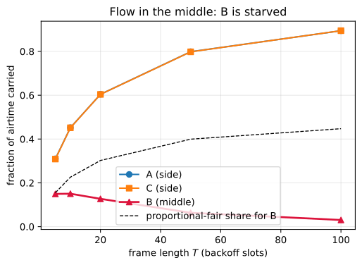
Simulated DCF throughput on the flow-in-the-middle conflict graph as the frame length grows relative to the contention window. The curves for A and C coincide exactly, so only C’s markers are visible; the middle session B falls far below the proportional-fair share of half a side session’s rate.
Problem 18.3 — Sensing asymmetry
Sensing asymmetry. Consider the “asymmetric sensing” topology in Figure 18.12(b), assuming RTS/CTS is enabled. Session A starts from station 1 to station 2, and session B from station 3 to station 4.
Figure 18.12(b) shows four stations. A solid arrow runs from station 1 to station 2 (session A) and a solid arrow runs from station 3 to station 4 (session B). There is exactly one dashed line in the figure, joining station 2 and station 3; a dashed line denotes interference as well as sensing. So station 2 and station 3 are within range of each other, and no other pair is: station 1 can neither sense nor be sensed by stations 3 and 4, and station 4 is out of range of stations 1 and 2. Consequently session B’s transmissions corrupt reception at station 2, while session A’s transmissions do not reach station 4 at all.
(a) Figure 18.18 shows the activity of session B: two grey frames on B’s time axis, with times \(t_1\), \(t_2\) and \(t_3\) all falling inside the first frame and \(t_4\) falling inside the second frame, the gaps between the marked times growing as one moves right. At time \(t_1\) station 1 senses the channel to be idle and sends an RTS frame to station 2 in an attempt to transmit data. What will happen?
(b) Suppose station 1 sends RTS frames at times \(t_2\), \(t_3\) and \(t_4\). What will happen? Roughly speaking, what is the relationship between the time differences \(t_2 - t_1\), \(t_3 - t_2\) and \(t_4 - t_3\)?
(c) Explain why it is difficult for session A to transmit successfully.
(d) Suppose we reverse the statuses of sessions A and B, i.e., session A is transmitting and station 3 sends an RTS frame to initiate data transfer in session B. Explain why the problem in part (c) disappears. (difficulty: \(\star\))
(a) The RTS dies at station 2 and no CTS returns; (b) the same, with the gaps doubling; (c) station 1 is blind and station 3 immune; (d) reversed, the CTS reaches the station that must defer.
The single edge \(2\)–\(3\) is the whole story: the station suffering the interference (2) hears the interferer (3), but the station that must act on it (1) hears nothing.
(a) Station 1 senses idle at \(t_1\) – as it does always, being out of range of 3 and 4 – but session B is mid-frame, so the RTS is destroyed at station 2 and no CTS returns. Station 1 waits out the CTS timeout, scores the attempt as a collision (Section 18.1.2: the missing reply is the only feedback), doubles its contention window and re-arms the counter.
(b) All three attempts fail exactly as in (a). After \(k\) failures station 1 draws its backoff uniformly from \(W_{\min}2^{k}\) slots, mean \(W_{\min}2^{k-1}\), so in expectation
\begin{equation*} \mathbb{E}[t_2 - t_1] \;\approx\; \tfrac{1}{2}\,\mathbb{E}[t_3-t_2] \;\approx\; \tfrac{1}{4}\,\mathbb{E}[t_4-t_3], \end{equation*}
i.e. the gaps grow geometrically with ratio about 2, as Figure 18.18 draws them.
(c) Station 1’s attempts are timed independently of B’s activity, so an RTS lands inside a B frame with probability about \(\rho_B\) and carrier sensing cannot help. Meanwhile A’s failures inflate A’s window while B never fails at all (station 1’s RTS cannot reach station 4), so B stays at \(W_{\min}\) and \(\rho_B\) rises as A’s attempt rate decays geometrically. RTS/CTS cannot repair this direction: the node to silence is station 3, only a CTS from station 2 can silence it, and station 2 can emit one only if station 3 is already quiet.
The simulation below uses \(W_{\min} = 16\), at most 6 doublings, a one-slot RTS and \(T = 20\)-slot data frames; station 1 never defers, station 3 defers only under a NAV set by station 2’s CTS, B’s frames destroy reception at station 2, and A’s never harm station 4.
import random
def asym(Wmin=16, Bmax=6, T=20, slots=2000000, seed=0, cts_heard=True):
# station 1 -> 2 is session A, station 3 -> 4 is session B
rng = random.Random(seed)
ctrA = rng.randrange(Wmin); ctrB = rng.randrange(Wmin)
stA = 0; dA = 0; dB = 0; nav = 0; badA = False
okA = 0; okB = 0; rtsA = 0
for _ in range(slots):
Bon = dB > 0
startB = (dB == 0 and nav == 0 and ctrB == 0)
startA = (dA == 0 and ctrA == 0) # station 1 senses nobody, never defers
if dA == 0 and ctrA > 0: ctrA -= 1
if dB == 0 and nav == 0 and ctrB > 0: ctrB -= 1
if startB: dB = T
if startA: # station 1 sends a one-slot RTS
rtsA += 1
if Bon or startB: # RTS wiped out at station 2
stA = min(stA+1, Bmax); ctrA = rng.randrange(Wmin * 2**stA)
else:
dA = T; badA = False
if cts_heard: nav = T + 1 # station 2's CTS silences station 3
if dA > 0 and (Bon or startB) and not startA: badA = True
if dA > 0:
dA -= 1
if dA == 0:
if badA: stA = min(stA+1, Bmax)
else: okA += 1; stA = 0
ctrA = rng.randrange(Wmin * 2**stA)
if dB > 0:
dB -= 1
if dB == 0: okB += 1; ctrB = rng.randrange(Wmin)
if nav > 0: nav -= 1
return T*okA/slots, T*okB/slots, rtsA, okA
for cts in (True, False):
a, b, r, o = asym(cts_heard=cts)
tag = "station 3 obeys the CTS" if cts else "station 3 never hears one"
print(f"{tag:26s}: A={a:.4f} B={b:.4f} A/B={a/b:.3f} "
f"({o} data frames out of {r} RTS attempts by station 1)")
station 3 obeys the CTS : A=0.0449 B=0.6954 A/B=0.065 (4488 data frames out of 16043 RTS attempts by station 1)
station 3 never hears one : A=0.0000 B=0.7279 A/B=0.000 (0 data frames out of 3939 RTS attempts by station 1)
Session A carries \(4.5\%\) of the airtime against B’s \(69.5\%\), the 1:15 ratio Section 18.4.1 predicts against a proportionally fair 1:1. The loss is almost all inflated contention window rather than per-attempt collision: station 1’s RTS succeeds on \(4488/16043 = 28\%\) of attempts (just B’s idle fraction) but it manages only one attempt per 125 slots against a minimum window of 16. Disabling station 3’s NAV response removes even that 4.5%, since its counter, drawn from \(\{0,\dots,15\}\), almost always cuts into A’s 20-slot frame.
(d) Reversed, A is already on the air, meaning station 2 decoded an RTS in one of B’s idle gaps and answered with a CTS. Station 3 is in range of station 2, so it heard that CTS and set its NAV for the data frame and ACK; when its backoff expires it defers instead of transmitting. The silencing message now travels along the one edge that exists, the station needing the information being precisely the CTS sender’s neighbour.
Problem 18.4 — Aloha
Aloha. There is a simpler random access protocol than CSMA that is just as famous. It is called Aloha, as it was invented in Hawaii in the early 1970s, and further led to the development of packet radio technologies. The operation of (the slotted time version of) Aloha is easy to describe. During each timeslot, each of a given set of \(N\) users chooses to transmit a packet with probability \(p\). We assume that if two or more users transmit at the same timeslot, all packets are lost. This is the only feedback available at each transmitter. Each lost packet is retransmitted with probability \(p\) too. We assume this process continues until a packet is eventually transmitted successfully.
(a) Assume the channel supports 1 unit of capacity (say, 1 Mbps) when there is a successful transmission. What is the throughput \(S\) as a function of \(N\) and \(p\)?
(b) What is the optimal \(p\), as a function of \(N\), to maximize the throughput?
(c) As the network becomes large and \(N \to \infty\), what is the maximized throughput? You will see it is not a big number, which is intuitive since slotted Aloha described above has neither the listen-and-wait nor the exponential backoff features. Aloha takes the least amount of communication and coordination and it does not even use carrier sensing. It also has a low throughput. CSMA leverages implicit message passing through carrier sensing but requires no further explicit coordination. Its throughput can be high for a very small number of users but drops as the crowd gets larger. A centralized scheduler would have incurred even more coordination overhead, and would in turn provide the best performance. But in many networks, it is infeasible to afford a centralized scheduler. (difficulty: \(\star\star\))
\(S = Np(1-p)^{N-1}\), maximized at \(p^\star = 1/N\), with \(S^\star \to 1/e \approx 0.368\).
(a) A slot is worth 1 unit exactly when one of the \(N\) independent users transmits, so
\begin{equation*} S(N,p) \;=\; \binom{N}{1} p (1-p)^{N-1} \;=\; N p (1-p)^{N-1} \quad \text{Mbps}, \end{equation*}
the Aloha counterpart of \(P_s P_t = N\tau(1-\tau)^{N-1}\) in (18.3) – with no division by an average slot length, since every Aloha slot has the same length.
(b) Differentiating,
\begin{equation*} \frac{\partial S}{\partial p} \;=\; N (1-p)^{N-2}\bigl[(1-p) - (N-1)p\bigr], \end{equation*}
and on \(0 < p < 1\) the bracket \(1 - Np\) is positive below \(p = 1/N\) and negative above, so
\begin{equation*} p^\star = \frac{1}{N} \end{equation*}
is the unique maximum (the endpoints give \(S = 0\)). Equivalently, aim for \(\mathbb{E}[\text{transmitters}] = Np = 1\) per slot – which requires each user to know \(N\), information this protocol does not have.
(c) Substituting,
\begin{equation*} S^\star(N) = \Bigl(1-\frac{1}{N}\Bigr)^{N-1} \longrightarrow \frac{1}{e} \approx 0.3679 \text{ Mbps}, \end{equation*}
since \((1-1/N)^N \to e^{-1}\) and \((1-1/N)^{-1} \to 1\). The approach is monotone from above (\(S^\star(2) = 0.5\), \(S^\star(10) = 0.387\)): in the limit \(1/e\) of slots sit empty and \(1 - 2/e \approx 26\%\) are lost to collisions, and no \(p\) recovers them.
import numpy as np
from scipy.optimize import minimize_scalar
S = lambda N, p: N * p * (1 - p)**(N - 1)
print(" N numerical argmax p 1/N S at optimum")
for N in (2, 3, 5, 10, 50, 1000):
r = minimize_scalar(lambda p: -S(N, p), bounds=(1e-9, 1 - 1e-9),
method='bounded', options={'xatol': 1e-12})
print(f"{N:5d} {r.x:.9f} {1/N:.9f} {S(N, r.x):.6f}")
print("limiting value (1 - 1/N)^(N-1) -> 1/e =", 1/np.e)
N numerical argmax p 1/N S at optimum
2 0.500000000 0.500000000 0.500000
3 0.333333331 0.333333333 0.444444
5 0.199999997 0.200000000 0.409600
10 0.099999996 0.100000000 0.387420
50 0.020000000 0.020000000 0.371602
1000 0.001000000 0.001000000 0.368063
limiting value (1 - 1/N)^(N-1) -> 1/e = 0.36787944117144233
import numpy as np
import matplotlib.pyplot as plt
p = np.linspace(1e-4, 1, 600)
plt.figure(figsize=(6, 4))
for N in (2, 5, 10, 50):
plt.plot(p, N * p * (1 - p)**(N - 1), label=f'N={N}')
plt.plot(1.0/N, (1 - 1.0/N)**(N - 1), 'k.')
plt.axhline(1/np.e, ls='--', c='gray')
plt.text(0.55, 1/np.e + 0.012, '$1/e=0.368$', color='gray')
plt.xlabel('transmission probability $p$')
plt.ylabel('throughput $S$ (Mbps)')
plt.title('Slotted Aloha throughput')
plt.legend(); plt.grid(alpha=.3)
plt.savefig('nl-ch18-aloha-throughput.svg', dpi=150, bbox_inches='tight')
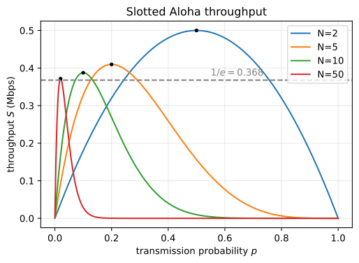
Slotted Aloha throughput against the per-user transmission probability. Each curve peaks at \(p=1/N\) (black dots), and the peak value falls monotonically towards the horizontal asymptote \(1/e\). The peaks also sharpen as \(N\) grows, so a large population is not only limited to 37% of the channel but is also increasingly sensitive to mis-setting \(p\).
Problem 18.5 — Alternative backoff rules
Alternative backoff rules. Suppose there are two stations in a CSMA network attempting to transmit a data frame. The two stations start at stage 1 with some contention window size \(w_1\), and each station chooses a timeslot within the contention window, uniformly at random. If the chosen timeslots collide, then the stations proceed to stage 2 with an updated contention window size \(w_2\), and so on. Transmission completes at some stage \(i\), if during this stage the two stations choose different timeslots. We are interested in the expected number of timeslots that will have elapsed before the completion of transmission. This expected number is a measure of how efficient the transmission is (the smaller the better).
To simplify the upcoming analysis, we assume there is no limit to the number of stages, i.e., the contention window size is unbounded.
(a) Suppose the two stations are in stage \(i\) with contention window size \(w_i\). What is the probability that the stations choose the same timeslot? Conditioning on the two stations having chosen the same timeslot, what is the expected value of the timeslot chosen, given that they are indexed from 1 to \(w_i\)?
(b) What is the probability that the transmission completes at stage \(i\)?
(c) Given that the transmission completes at stage \(i\), what is the expected number of timeslots elapsed? (Hint: It is the sum of the expected values of timeslots chosen in previous stages (see part (a)), plus the expected value of the maximum of the two (different) timeslots chosen at stage \(i\), which is \(2(w_i + 1)/3\).)
(d) What is the expected number of timeslots elapsed before the completion of transmission? (Hint: Apply the law of total expectation.)
(e) Now we plug in different contention window update rules. Consider the following three rules: (1) binary exponential backoff, \(w_i = 2^i\); (2) additive backoff, \(w_i = i\); (3) super-binary exponential backoff, \(w_i = 2^{2i}\). Compute the expected number of timeslots in part (d) for the three cases. What do you observe? How does that match the intuition that the best backoff policy should be neither too conservative nor too aggressive? (difficulty: \(\star\star\star\))
(a) \(1/w_i\) and \((w_i+1)/2\); (b) \(\bigl(\prod_{j<i} 1/w_j\bigr)(1-1/w_i)\); (c)–(d) below; (e) binary backoff wins at 4.24 slots.
Let \(X_i, Y_i\) be the stage-\(i\) draws, independent and uniform on \(\{1,\dots,w_i\}\). A collided stage costs \(X_j = Y_j\) slots and the final stage costs \(\max(X_i,Y_i)\), the transmission completing only once the later station has had its turn.
(a) \(\Pr[X_i = Y_i] = \sum_{k} w_i^{-2} = 1/w_i\), and each \(k\) contributes the same \(1/w_i^2\) to that event, so the common value is uniform and \(\mathbb{E}[X_i \mid X_i = Y_i] = (w_i+1)/2\).
(b) Stages are independent, so completing at stage \(i\) is colliding at \(1,\dots,i-1\) and not at \(i\):
\begin{equation*} \Pr[I = i] \;=\; \Bigl(\prod_{j=1}^{i-1}\frac{1}{w_j}\Bigr)\Bigl(1 - \frac{1}{w_i}\Bigr), \end{equation*}
a proper distribution whenever \(w_j \ge 2\) eventually, as all three rules of (e) satisfy.
(c) The elapsed slots are \(\sum_{j<i}X_j + \max(X_i,Y_i)\), so by linearity and (a),
\begin{equation*} \mathbb{E}[T \mid I=i] \;=\; \sum_{j=1}^{i-1}\frac{w_j+1}{2} \;+\; \frac{2(w_i+1)}{3}. \end{equation*}
For the last term, write \(w = w_i\); since \(\Pr[\max = k] = (2k-1)/w^2\),
\begin{align*} \mathbb{E}[\max] &= \frac{1}{w^2}\sum_{k=1}^{w}k(2k-1) = \frac{(w+1)(4w-1)}{6w}, \\ \mathbb{E}[\max] &= \frac{1}{w}\cdot\frac{w+1}{2}
- \Bigl(1-\frac1w\Bigr)\mathbb{E}[\max \mid X\ne Y], \end{align*}
and solving the second for the conditional mean gives \(2(w+1)/3\), the hint’s value.
(d) Total expectation over the completion stage gives
\begin{equation*} \mathbb{E}[T] = \sum_{i=1}^{\infty} \Bigl(\prod_{j=1}^{i-1}\frac{1}{w_j}\Bigr)\Bigl(1-\frac{1}{w_i}\Bigr) \left[\sum_{j=1}^{i-1}\frac{w_j+1}{2} + \frac{2(w_i+1)}{3}\right], \end{equation*}
a tug of war: fast-growing \(w_i\) collapses the prefactor so few stages are reached, but inflates the \(2(w_i+1)/3\) actually paid at the successful stage.
(e) The series converges fast (the binary prefactor is \(2^{-i(i-1)/2}\)), so a few dozen terms suffice.
def expected_slots(w, imax=2000):
total = 0.0; prod = 1.0; before = 0.0; mass = 0.0; stages = 0.0
for i in range(1, imax + 1):
wi = w(i)
P = prod * (1 - 1.0 / wi) # collide in 1..i-1, differ at i
total += P * (before + 2 * (wi + 1) / 3.0)
mass += P; stages += i * P
before += (wi + 1) / 2.0 # slots burnt by the collision at stage i
prod /= wi
if prod < 1e-300:
break
return total, mass, stages
rules = [("binary w_i = 2^i ", lambda i: 2.0**i),
("additive w_i = i ", lambda i: float(i)),
("super-binary w_i = 4^i ", lambda i: 4.0**i)]
for name, w in rules:
e, m, s = expected_slots(w)
print(f"{name}: E[slots] = {e:.4f} E[stages] = {s:.4f} (total prob {m:.12f})")
binary w_i = 2^i : E[slots] = 4.2361 E[stages] = 1.6416 (total prob 1.000000000000)
additive w_i = i : E[slots] = 4.6971 E[stages] = 2.7183 (total prob 1.000000000000)
super-binary w_i = 4^i : E[slots] = 6.6309 E[stages] = 1.2659 (total prob 1.000000000000)
Binary exponential backoff wins at 4.24 slots; additive costs 11% more and super-binary 57% more, for opposite reasons. Additive is too aggressive – its windows are tiny (\(w_1 = 1\) makes stage 1 a certain collision), so stages are cheap but numerous, 2.7183 expected against binary’s 1.64. Super-binary is too conservative – 1.27 expected stages, but reaching stage 2 already means a window of 16 and an expected wait of \(2\cdot17/3 \approx 11.3\) slots there alone. Sweeping \(w_i = a^i\) makes the tradeoff visible.
import numpy as np
from scipy.optimize import minimize_scalar
def ET(w, imax=2000):
total = 0.0; prod = 1.0; before = 0.0
for i in range(1, imax + 1):
wi = w(i); P = prod * (1 - 1.0 / wi)
total += P * (before + 2 * (wi + 1) / 3.0)
before += (wi + 1) / 2.0; prod /= wi
if prod < 1e-300: break
return total
r = minimize_scalar(lambda x: ET(lambda i, x=x: x**i), bounds=(1.05, 8), method='bounded')
print(f"best multiplier a* = {r.x:.4f} with E[slots] = {r.fun:.4f}")
for a in (1.05, 1.2, 1.5, 2.0, 3.0, 4.0, 8.0):
print(f" a = {a:4.2f}: E[slots] = {ET(lambda i, a=a: a**i):.4f}")
best multiplier a* = 1.4984 with E[slots] = 3.9275
a = 1.05: E[slots] = 6.7657
a = 1.20: E[slots] = 4.3699
a = 1.50: E[slots] = 3.9275
a = 2.00: E[slots] = 4.2361
a = 3.00: E[slots] = 5.3674
a = 4.00: E[slots] = 6.6309
a = 8.00: E[slots] = 11.8861
import numpy as np
import matplotlib.pyplot as plt
def ET(w, imax=2000):
total = 0.0; prod = 1.0; before = 0.0
for i in range(1, imax + 1):
wi = w(i); P = prod * (1 - 1.0 / wi)
total += P * (before + 2 * (wi + 1) / 3.0)
before += (wi + 1) / 2.0; prod /= wi
if prod < 1e-300: break
return total
a = np.linspace(1.05, 8, 400)
E = [ET(lambda i, a=a_: a_**i) for a_ in a]
plt.figure(figsize=(6, 4))
plt.plot(a, E, lw=2)
plt.plot(1.4984, 3.9275, 'o', color='crimson')
plt.annotate('$a^*=1.50$', (1.4984, 3.9275), textcoords='offset points', xytext=(8, 10))
for a_, lab in ((2, 'binary ($a=2$)'), (4, 'super-binary ($a=4$)')):
plt.plot(a_, ET(lambda i, a_=a_: a_**i), 's', color='k')
plt.annotate(lab, (a_, ET(lambda i, a_=a_: a_**i)),
textcoords='offset points', xytext=(6, -16))
plt.axhline(4.6971, ls='--', c='gray')
plt.text(6.0, 4.80, 'additive $w_i=i$', color='gray')
plt.xlabel('backoff multiplier $a$ in $w_i = a^i$')
plt.ylabel('expected timeslots to completion')
plt.title('Too aggressive versus too conservative')
plt.grid(alpha=.3)
plt.savefig('nl-ch18-backoff-multiplier.svg', dpi=150, bbox_inches='tight')
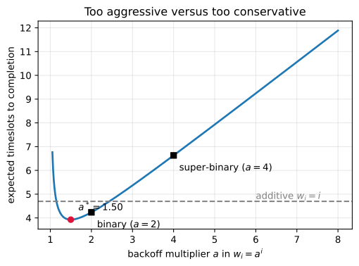
Expected timeslots to complete both transmissions under the geometric rule \(w_i = a^i\), for two stations. The curve is U-shaped: it blows up as \(a \to 1\) (windows too small, endless collisions) and grows linearly for large \(a\) (windows too big, endless waiting). Binary backoff sits just to the right of the minimum at \(a^* \approx 1.5\); super-binary sits far out on the conservative arm, and additive backoff (dashed line) is worse than every geometric rule with \(1.15 \lesssim a \lesssim 2.4\).
The cost is U-shaped in aggressiveness, as Section 18.3.2 states: collisions on one arm, silence on the other. The minimum sits at \(a^\star \approx 1.50\), so binary backoff is near-optimal rather than optimal in this two-station unbounded-window model; real DCF faces an unknown and varying \(N\) under \(W_{\min} = 15\), \(B = 3\), and a multiplier of 2 is the standard’s parameter-free hedge across that range.
Why am I getting only a few of the advertised 4G speed?
Problem 19.1 — RTS/CTS overhead
RTS/CTS overhead.
In the Examples section of Chapter 18, we estimated \(T_s\) of 802.11g at 54 Mbps for the case in which RTS/CTS is disabled. Here we estimate \(T_s\) for the other case. Given that RTS/CTS is enabled, a successful transmission consists of the sequence [RTS frame] + SIFS + [CTS frame] + SIFS + [data frame] + SIFS + [ACK frame] + DIFS. The only addition is the RTS/CTS handshake that occurs before data transmission.
You are also given that (1) the time taken to transmit an RTS frame is 23.25 us, and (2) the time taken to transmit a CTS frame is 22.37 us.
(a) If \(L = 8192\) bits, calculate \(T_s\) both for the case of RTS/CTS being enabled and for the case of RTS/CTS being disabled. Calculate the effective throughput as \(L/T_s\).
(b) If \(L = 320\) bits, calculate \(T_s\) and \(L/T_s\) for both cases again.
(c) In most home networks, RTS/CTS is disabled. Can you see why from (a) and (b)? (difficulty: \(\star\))
RTS/CTS costs a payload-independent \(\Delta = 65.62\) us, so its relative price falls as \(L\) grows: 21.7% at \(L = 8192\) bits, 41.7% at \(L = 320\).
With Section 18.3.1’s 802.11g constants (slot 9 us, SIFS 10 us, DIFS 28 us), the data frame carries a 16 us preamble, a 40-bit PHY header split across 6 and 54 Mbps, a 240-bit MAC header and a 32-bit CRC, and the ACK takes \(16 + 24/6 + (16+112)/54 = 22.37\) us, so
\begin{align*} T_{\text{data}}(L) &= 16 + \tfrac{24}{6} + \tfrac{16+240+32}{54} + \tfrac{L}{54} = 25.33 + \tfrac{L}{54},\\ T_s^{\text{off}}(L) &= T_{\text{data}} + \text{SIFS} + T_{\text{ACK}} + \text{DIFS} = 85.70 + \tfrac{L}{54} \ \text{us}. \end{align*}
Enabling the handshake prepends [RTS] + SIFS + [CTS] + SIFS, so
\begin{equation*} \Delta = 23.25 + 10 + 22.37 + 10 = 65.62, \qquad T_s^{\text{on}}(L) = 151.32 + \tfrac{L}{54} \ \text{us}. \end{equation*}
SIFS, DIFS = 10.0, 28.0
T_ACK, T_CTS, T_RTS = 22.37, 22.37, 23.25
def T_data(L): return 25.33 + L/54.0
def Ts_off(L): return T_data(L) + SIFS + T_ACK + DIFS
def Ts_on(L): return T_RTS + SIFS + T_CTS + SIFS + T_data(L) + SIFS + T_ACK + DIFS
for L in (8192, 320):
off, on = Ts_off(L), Ts_on(L)
print(f"L = {L} bits")
print(f" RTS/CTS off: Ts = {off:.2f} us, L/Ts = {L/off:.3f} Mbps ({100*L/off/54:.1f}% of 54)")
print(f" RTS/CTS on : Ts = {on:.2f} us, L/Ts = {L/on:.3f} Mbps ({100*L/on/54:.1f}% of 54)")
print(f" handshake cost = {on-off:.2f} us, throughput loss = {100*(1-(L/on)/(L/off)):.1f}%")
L = 8192 bits
RTS/CTS off: Ts = 237.40 us, L/Ts = 34.507 Mbps (63.9% of 54)
RTS/CTS on : Ts = 303.02 us, L/Ts = 27.034 Mbps (50.1% of 54)
handshake cost = 65.62 us, throughput loss = 21.7%
L = 320 bits
RTS/CTS off: Ts = 91.63 us, L/Ts = 3.492 Mbps (6.5% of 54)
RTS/CTS on : Ts = 157.25 us, L/Ts = 2.035 Mbps (3.8% of 54)
handshake cost = 65.62 us, throughput loss = 41.7%
Collected, (a) in the first row and (b) in the second:
| \(L\) (bits) | \(T_s\) off (us) | \(L/T_s\) off (Mbps) | \(T_s\) on (us) | \(L/T_s\) on (Mbps) |
|---|---|---|---|---|
| 8192 | 237.40 | 34.51 | 303.02 | 27.03 |
| 320 | 91.63 | 3.49 | 157.25 | 2.04 |
(c) RTS/CTS buys only cheap collisions – \(T_c\) drops from a full \(T_s = 237.40\) us to \(T_{\text{RTS}} + \text{DIFS} = 51.25\) us – plus protection against hidden terminals, and it pays \(\Delta\) on every success. It therefore wins only when collisions are frequent and frames are long, and a home network has neither property: two or three stations all in earshot, and traffic full of short frames on which (b) shows the handshake alone costs 42%.
Quantifying “frequent”, the Chapter 18 renewal model (18.4) with \(\tau\) from (18.5) and (18.7), altering only \(T_c\), gives the crossovers below. (Solving the printed (18.7) with \(W_{\min} = 15\), \(B = 3\) gives \(\tau = 0.0814\) at \(N = 5\) where Section 18.3.2 quotes \(0.0765\); the discrepancy moves the crossover by at most one station.)
import numpy as np
from scipy.optimize import brentq
Tb, Wmin, B = 28.0, 15, 3
def solve_tau(N):
def f(tau):
c = 1 - (1-tau)**(N-1)
s = sum(c**i * 2**(i-1) * Wmin for i in range(B+1))
return tau - 1.0/(1 + (1-c)/(1-c**(B+1)) * s)
return brentq(f, 1e-9, 0.3)
def S(N, L, rts):
tau = solve_tau(N)
Ts = Ts_on(L) if rts else Ts_off(L)
Tc = (T_RTS + DIFS) if rts else Ts
succ = N*tau*(1-tau)**(N-1)
idle = (1-tau)**N
coll = 1 - idle - succ
return succ*L/(idle*Tb + coll*Tc + succ*Ts) # L in bits, times in us -> Mbps
print("L = 8192 bits")
print(" N tau S_off(Mbps) S_on(Mbps)")
for N in [2,3,5,10,20,30,50]:
print(f"{N:3d} {solve_tau(N):.4f} {S(N,8192,False):8.2f} {S(N,8192,True):8.2f}")
print()
for L in (16384, 8192, 320):
xs = [N for N in range(2,60) if S(N,L,True) > S(N,L,False)]
print(f"L={L}: RTS/CTS wins for N >= {xs[0] if xs else 'never (N<60)'}")
L = 8192 bits
N tau S_off(Mbps) S_on(Mbps)
2 0.1054 22.13 19.28
3 0.0954 23.28 20.63
5 0.0814 23.64 21.78
10 0.0636 22.38 22.56
20 0.0499 19.07 22.42
30 0.0440 16.03 21.67
50 0.0387 11.01 19.35
L=16384: RTS/CTS wins for N >= 6
L=8192: RTS/CTS wins for N >= 10
L=320: RTS/CTS wins for N >= 43
For 1 kB frames the crossover is \(N \approx 10\), well above a home network’s 2 to 5 stations, where turning RTS/CTS off is worth 2 to 3 Mbps. The model assumes every station hears every other, so it credits the handshake only with shortening collisions; hidden terminals push the crossover far lower, which is why the deployed rule is a per-frame RTS threshold (default 2347 bytes, effectively never) rather than a global switch.
Problem 19.2 — Header overhead
Header overhead.
A typical IEEE 802.3 Ethernet packet structure is illustrated in Figure 19.8, with the terminology explained below. Figure 19.8 shows two nested layers. The Ethernet packet, read left to right, is: Preamble (8 bytes), MAC Dest (6 bytes), MAC Src (6 bytes), Length (2 bytes), a variable field holding the packet from the IP layer (typically 46 to 1500 bytes), CRC (4 bytes), and Interframe Gap (12 bytes). The variable field is expanded below it as the TCP packet: IPv6 header (40 bytes), TCP header (20 bytes), and a variable field holding the packet from the session layer (at most 65536 bytes).
- Preamble: Uses 64 bits to synchronize with the signal’s frequency before transmitting the real data.
- MAC Dest/Src: Records the destination and source MAC addresses of the packet, each with 6 bytes.
- Length: Specifies the length of the IP packet with 2 bytes.
- Frame-check sequence: Contains a 32-bit cyclic redundancy check that enables the detection of corrupted data within the packet.
- Inter-frame gap: After a packet has been sent, transmitters are required to transmit a total of 96 bits of “idle line” state before transmitting the next packet.
- IPv6 header: 40 bytes in total.
- TCP header: 20 bytes in total.
What is the percentage of payload data rate if we are to send a 250-byte packet? (difficulty: \(\star\))
\(190/288 = 65.97\%\).
Framing around the IP packet costs
\begin{equation*} 8_{\text{preamble}} + 6_{\text{dest}} + 6_{\text{src}} + 2_{\text{length}}
- 4_{\text{CRC}} + 12_{\text{IFG}} = 38 \text{ bytes}, \end{equation*}
the inter-frame gap included since the transmitter may send nothing else during it, and the IPv6 and TCP headers cost \(40 + 20 = 60\) more. Figure 19.8 labels the field handed down from the IP layer “packet”, so the 250 bytes is the IP packet and
\begin{equation*} \frac{250 - 60}{250 + 38} = \frac{190}{288} = 65.97\% . \end{equation*}
(Reading the 250 bytes as session-layer data instead gives \(250/348 = 71.84\%\).)
PREAMBLE, MAC_D, MAC_S, LEN, CRC, IFG = 8, 6, 6, 2, 4, 12
ETH = PREAMBLE + MAC_D + MAC_S + LEN + CRC + IFG
IPV6, TCP = 40, 20
print("Ethernet/PHY framing overhead =", ETH, "bytes")
print("IPv6 + TCP headers =", IPV6 + TCP, "bytes")
ip_pkt = 250
payload = ip_pkt - IPV6 - TCP
wire = ETH + ip_pkt
print(f"\nReading A: the 250-byte packet is the IP packet (Ethernet payload field)")
print(f" application payload = {payload} bytes, bytes on wire = {wire}")
print(f" efficiency = {payload}/{wire} = {100*payload/wire:.2f}%")
app = 250
ip2 = app + IPV6 + TCP
wire2 = ETH + ip2
print(f"\nReading B: the 250 bytes are application data")
print(f" IP packet = {ip2} bytes, bytes on wire = {wire2}")
print(f" efficiency = {app}/{wire2} = {100*app/wire2:.2f}%")
Ethernet/PHY framing overhead = 38 bytes
IPv6 + TCP headers = 60 bytes
Reading A: the 250-byte packet is the IP packet (Ethernet payload field)
application payload = 190 bytes, bytes on wire = 288
efficiency = 190/288 = 65.97%
Reading B: the 250 bytes are application data
IP packet = 310 bytes, bytes on wire = 348
efficiency = 250/348 = 71.84%
In general, with \(x\) the IP packet size in bytes, \(\eta(x) = (x-60)/(x+38)\), zero at \(x = 60\) and rising hyperbolically toward 1.
import numpy as np, matplotlib.pyplot as plt
ETH, HDR = 38, 60
ip = np.arange(60+1, 1501) # IP packet size, bytes
eff = 100*(ip - HDR)/(ip + ETH)
fig, ax = plt.subplots(figsize=(7,4.2))
ax.plot(ip, eff, lw=2, color='#1f77b4')
ax.axvline(250, ls='--', c='0.5'); ax.axhline(65.97, ls='--', c='0.5')
ax.plot([250],[65.97],'o',color='#d62728',zorder=5)
ax.annotate('250 B packet: 65.97%', xy=(250,65.97), xytext=(430,50),
arrowprops=dict(arrowstyle='->',color='#d62728'), color='#d62728')
ax.plot([1500],[100*(1500-HDR)/(1500+ETH)],'o',color='#2ca02c',zorder=5)
ax.annotate('1500 B (MTU): %.1f%%'%(100*(1500-HDR)/(1500+ETH)), xy=(1500,93.5), xytext=(900,80),
arrowprops=dict(arrowstyle='->',color='#2ca02c'), color='#2ca02c')
ax.set_xlabel('IP packet size (bytes)'); ax.set_ylabel('payload fraction of wire time (%)')
ax.set_title('IEEE 802.3 + IPv6 + TCP: useful fraction vs packet size')
ax.grid(alpha=.3); ax.set_ylim(0,100)
plt.savefig('nl-ch19-header-overhead.svg', dpi=150, bbox_inches='tight')
for s in (100,250,576,1500):
print(f"IP packet {s:4d} B -> payload {s-HDR:4d} B, wire {s+ETH:4d} B, efficiency {100*(s-HDR)/(s+ETH):5.2f}%")
IP packet 100 B -> payload 40 B, wire 138 B, efficiency 28.99%
IP packet 250 B -> payload 190 B, wire 288 B, efficiency 65.97%
IP packet 576 B -> payload 516 B, wire 614 B, efficiency 84.04%
IP packet 1500 B -> payload 1440 B, wire 1538 B, efficiency 93.63%
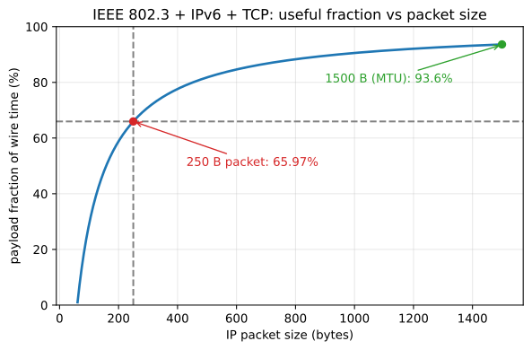
Fraction of Ethernet wire time carrying application payload, as a function of IP packet size, for IPv6 + TCP over IEEE 802.3. The 98 bytes of fixed overhead per packet cost 34% at the 250-byte point of this problem and only 6.4% at the 1500-byte MTU.
The 98 fixed bytes cost 34% here and only 6.4% at the 1500-byte MTU, which is why Nagle’s algorithm (Section 19.3.2) coalesces small writes, and why LTE’s PDCP sublayer compresses headers.
Problem 19.3 — The slow start phase’s throughput
The slow start phase’s throughput.
As mentioned in Chapter 14, TCP starts with a small congestion window, which is initially set to 1 MSS, and go through the slow start phase. The congestion window increases multiplicatively, e.g., 2 MSSs, 4 MSSs, 8 MSSs, …, for every round trip time, until the slow start threshold is reached and the congestion avoidance phase is entered. Suppose you open a web browser and try to download a webpage of 70 MSSs.
(a) Assuming there is no packet lost, how many RTTs are required in order to download the webpage? Remember to add up one RTT of handshake to set up the TCP connection.
(b) If RTT = 100 ms, what is the average throughput in kbps? Can you see the impact of slow start on a short-duration session’s throughput? (difficulty: \(\star\star\))
(a) 8 RTTs; (b) 1022 kbps.
(a) Slow start gives \(\text{cwnd}_k = 2^{k-1}\) MSS in the \(k\)-th data RTT, so \(n\) RTTs deliver \(\sum_{k=1}^{n}2^{k-1} = 2^n - 1\) MSS. Then \(2^n - 1 \ge 70\) needs \(n \ge \log_2 71 = 6.15\), i.e. \(n = 7\) data RTTs (the seventh sends only \(70 - 63 = 7\) of its 64 MSS), plus one RTT for the three-way handshake of Figure 19.1(a): 8 RTTs.
def slow_start(F):
cwnd, sent, r, rows = 1, 0, 0, []
while sent < F:
r += 1
this = min(cwnd, F - sent)
sent += this
rows.append((r, cwnd, this, sent))
cwnd *= 2
return rows
rows = slow_start(70)
print(" RTT cwnd sent cumulative")
for r, w, s, c in rows:
print(f"{r:4d} {w:4d} {s:4d} {c:10d}")
n_data = rows[-1][0]
print(f"\ndata RTTs = {n_data}, plus 1 handshake RTT -> {n_data+1} RTTs total")
RTT, MSS = 0.100, 1460
T = (n_data + 1)*RTT
bits = 70*MSS*8
print(f"total time = {T:.1f} s, bits = {bits}")
print(f"average throughput = {bits/T/1e3:.1f} kbps = {bits/T/1e6:.3f} Mbps")
ideal = bits/(2*RTT)
print(f"if cwnd were already >= 70 MSS: {ideal/1e3:.1f} kbps ({ideal/(bits/T):.2f}x higher)")
print(f"peak instantaneous rate in last full RTT (cwnd=64): {64*MSS*8/RTT/1e6:.2f} Mbps")
RTT cwnd sent cumulative
1 1 1 1
2 2 2 3
3 4 4 7
4 8 8 15
5 16 16 31
6 32 32 63
7 64 7 70
data RTTs = 7, plus 1 handshake RTT -> 8 RTTs total
total time = 0.8 s, bits = 817600
average throughput = 1022.0 kbps = 1.022 Mbps
if cwnd were already >= 70 MSS: 4088.0 kbps (4.00x higher)
peak instantaneous rate in last full RTT (cwnd=64): 7.48 Mbps
(The clock stops when the last window has been launched and acknowledged; stopping half an RTT earlier would give 7.5.)
(b) With Section 19.3.2’s MSS of 1460 bytes the page is \(70 \times 1460 \times 8 = 817\,600\) bits over \(8 \times 0.1 = 0.8\) s, so
\begin{equation*} \frac{817\,600}{0.8} = 1\,022\,000 \text{ bps} = 1022 \text{ kbps}. \end{equation*}
The impact is severe and has three parts: the handshake RTT carries no data (a 12.5% haircut); the ramp averages only \(70/7 = 10\) MSS per RTT against an eventual entitlement of 64, so an already-open window would finish in 0.2 s at 4088 kbps, exactly \(4\times\) faster; and the final RTT wastes 57 of its 64 MSS. In the last full RTT the sender pushes 7.48 Mbps while the session averages 1.02 Mbps – for a short flow the bottleneck is \(\text{cwnd}\), not the link.
import numpy as np, matplotlib.pyplot as plt
RTT, MSS = 0.100, 1460
def rtts(F):
cwnd, sent, r = 1, 0, 0
while sent < F:
r += 1; sent += min(cwnd, F-sent); cwnd *= 2
return r
Fs = np.arange(1, 4001)
thr = np.array([F*MSS*8/((rtts(F)+1)*RTT)/1e3 for F in Fs])
fig, ax = plt.subplots(figsize=(7.2,4.2))
ax.plot(Fs, thr, lw=1.6, color='#1f77b4')
ax.plot([70], [70*MSS*8/(8*RTT)/1e3], 'o', color='#d62728', zorder=5)
ax.annotate('70 MSS webpage:\n1022 kbps', xy=(70, 1022), xytext=(4, 4000),
arrowprops=dict(arrowstyle='->', color='#d62728'), color='#d62728')
ax.set_xscale('log'); ax.set_yscale('log'); ax.set_xlabel('webpage size (MSS)')
ax.set_ylabel('average throughput (kbps)')
ax.set_title('Slow start: average throughput vs transfer size (RTT = 100 ms)')
ax.grid(alpha=.3, which='both')
plt.savefig('nl-ch19-slow-start-throughput.svg', dpi=150, bbox_inches='tight')
for F in (1, 10, 70, 500, 4000):
print(f"F = {F:5d} MSS: {rtts(F)+1:3d} RTTs, avg throughput = {F*MSS*8/((rtts(F)+1)*RTT)/1e3:8.1f} kbps")
F = 1 MSS: 2 RTTs, avg throughput = 58.4 kbps
F = 10 MSS: 5 RTTs, avg throughput = 233.6 kbps
F = 70 MSS: 8 RTTs, avg throughput = 1022.0 kbps
F = 500 MSS: 10 RTTs, avg throughput = 5840.0 kbps
F = 4000 MSS: 13 RTTs, avg throughput = 35938.5 kbps
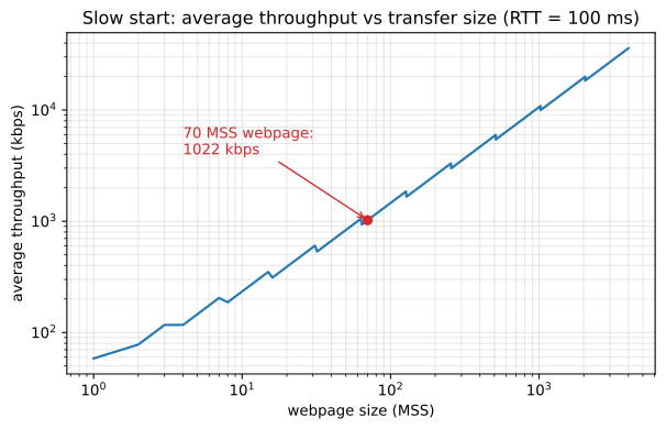
Average throughput of a loss-free slow-start transfer against transfer size, RTT = 100 ms, MSS = 1460 bytes, one handshake RTT included. Because the RTT count grows only like \(\log_2 F\), throughput rises almost linearly with \(F\) on the log-log axes; the sawtooth steps are the wasted final window just after each doubling.
Since the RTT count grows like \(\log_2 F\), throughput grows almost linearly with transfer size: 58 kbps for a 1-MSS request and 36 Mbps for a 6 MB file over the identical path. Web browsing lives on the left of that curve, which is what HTTP/2 multiplexing, a 10-MSS initial window (\(10+20+40 = 70\) would cut this transfer to 3 data RTTs) and QUIC’s 0-RTT handshake all target.
Problem 19.4 — Alternatives to indirect forwarding
Alternatives to indirect forwarding.
Section 19.4.2 mentioned the process of indirect forwarding in mobility management. Can you think of an alternative forwarding method? (difficulty: \(\star\star\))
Yes: direct forwarding with a cached binding. The correspondent \(B\) pays one lookup to the home agent at session start, learns \(A\)’s care-of address, caches it, and sends every later packet straight to the foreign agent; the home agent stays the rendezvous point, since it alone is reachable at \(A\)’s permanent ID, but stops relaying. This is Mobile IPv6 route optimisation.
Indirect forwarding sends every packet \(B \to \text{HA} \to \text{FA} \to A\) (Figure 19.3), so a home agent on another continent costs latency on every packet, burns the home access link, and makes itself a single point of failure for a session unrelated to the home network. Placing \(B\), HA and FA uniformly on a unit square with latency proportional to distance measures the dogleg.
import numpy as np, matplotlib.pyplot as plt
rng = np.random.default_rng(19)
M = 200000
B = rng.random((M,2)); HA = rng.random((M,2)); FA = rng.random((M,2))
d = lambda P,Q: np.linalg.norm(P-Q, axis=1)
ind = d(B,HA) + d(HA,FA) # indirect forwarding: B -> HA -> FA
dir_ = d(B,FA) # direct forwarding: B -> FA
stretch = ind/dir_
print(f"mean stretch = {stretch.mean():.3f}")
print(f"median stretch= {np.median(stretch):.3f}")
print(f"P(stretch>2) = {(stretch>2).mean():.3f}")
print(f"P(stretch>3) = {(stretch>3).mean():.3f}")
print(f"mean latency: indirect {ind.mean():.3f}, direct {dir_.mean():.3f} (units of cell width)")
# one binding lookup costs a round trip to the home agent; amortise it over n packets
nstar = 2*d(B,HA)/(ind - dir_)
print(f"\nbreak-even session length (packets) for direct forwarding:")
print(f" median n* = {np.median(nstar):.2f}, 90th pct = {np.quantile(nstar,0.9):.2f}, P(n*<=1) = {(nstar<=1).mean():.3f}")
fig, ax = plt.subplots(figsize=(7,4.2))
ax.hist(np.clip(stretch,1,6), bins=np.linspace(1,6,101), color='#1f77b4', alpha=.85)
ax.axvline(np.median(stretch), color='#d62728', lw=2,
label=f'median stretch = {np.median(stretch):.2f}')
ax.axvline(1.0, color='k', lw=1, ls='--', label='direct forwarding = 1.00')
ax.set_xlabel('latency stretch of indirect over direct forwarding')
ax.set_ylabel('count (200 000 random placements)')
ax.set_title('Triangle-routing penalty, agents uniform on a unit square')
ax.legend(); ax.grid(alpha=.3)
plt.savefig('nl-ch19-triangle-routing-stretch.svg', dpi=150, bbox_inches='tight')
mean stretch = 3.033
median stretch= 1.859
P(stretch>2) = 0.455
P(stretch>3) = 0.256
mean latency: indirect 1.043, direct 0.522 (units of cell width)
break-even session length (packets) for direct forwarding:
median n* = 2.00, 90th pct = 15.86, P(n*<=1) = 0.000
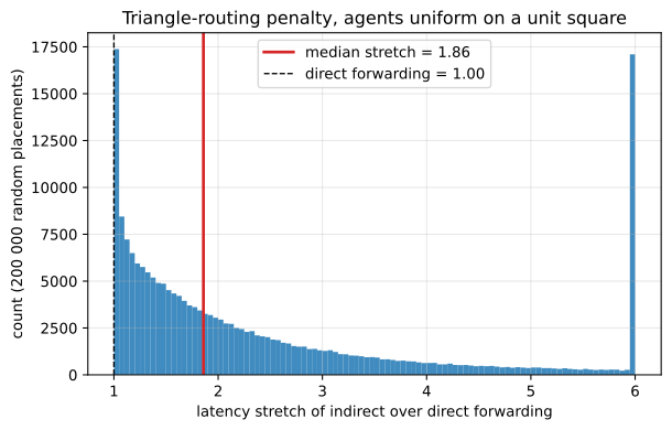
Distribution of the indirect/direct latency ratio over 200 000 random placements of correspondent, home agent and foreign agent. Values above 6 are clipped into the rightmost bin. Indirect forwarding doubles the mean one-way latency and exceeds a 2x penalty in 46% of placements.
Indirect forwarding doubles the mean one-way latency and exceeds \(2\times\) in 46% of placements. Under Section 19.3.2’s window-limited model throughput is window/RTT, so that doubling halves throughput, while the fix costs one binding lookup and breaks even at a median of two packets.
The price is that state and trust move out to the correspondent. Every correspondent must be mobility-aware, where the home agent need only be upgraded once. Binding updates must be authenticated by a party that shares no security association with \(A\), so an unauthenticated “\(A\) has moved to \(X\)” is a redirection and amplification attack; Mobile IPv6 patches this with return routability, at extra round trips and weak assurance. And handover becomes a binding update to every active correspondent rather than one table entry, so for a fast-moving user the signalling can exceed the saving.
That last cost is why the deployed answer is neither extreme but hierarchical anchoring: a local anchor absorbs the frequent short-range handovers so the global binding rarely changes – Hierarchical and Proxy Mobile IPv6, and Section 19.4.1’s S-GW buffering data as a local mobility anchor while the P-GW holds the stable address. The alternatives that avoid forwarding entirely are dynamic re-addressing by DHCP (abandoning session continuity), the identifier/locator split of HIP and LISP (principled, but it needs a new global mapping infrastructure), and transport-layer migration in MPTCP and QUIC, which shipped precisely because it needs no new network element.
Problem 19.5 — Overhead associated with security
Overhead associated with security.
We have not had a chance to talk about network security so far, a significant subject with many books written about it. There are several meanings to the word “security,” and many famous methods to ensure or to break security in a network. We will simply walk through the main steps involved in ensuring confidentiality in Secure SHell (SSH), an application-layer security protocol heavily used in remote login to ensure that the server is the right one, the client is who it claims to be, and the communication between this client and the server is confidential. Along the way, we will see the amount of overhead involved in providing SSH’s secure service.
There are numerous books and papers about encrypting texts. We will need only the following notion in this homework problem: public key cryptography. This is based on mathematical operations that are easy to run one way but very difficult the other way around, e.g., multiplying two large prime numbers is easy, but factoring a large number into two large prime numbers is very difficult. This enables the creation of a pair of keys: a public encryption key (known to anyone who wants to send a message to, say, Alice), and a private decryption key (known only to those who are allowed to decrypt and read the original message).
Now consider a client trying to remotely login to a server. If you are the inventor of a secure remote login protocol using public and private keys, what are the steps you would design? What would be the biggest vulnerability of your design? (difficulty: \(\star\star\star\))
The design below is essentially SSH, and its biggest vulnerability is the trust bootstrap: the client must decide whether the public key it was just handed belongs to the server it meant to reach, and every other guarantee is conditional on that unverifiable decision.
The design, in six steps.
- Long-term keys. The server generates a host key pair \((\text{pk}_S, \text{sk}_S)\); the client generates \((\text{pk}_C, \text{sk}_C)\) and deposits \(\text{pk}_C\) on the server out of band. The asymmetry is the whole problem: the client’s key reaches the server by a trusted channel, the server’s key has none.
- Negotiation. Both sides announce version, cipher, MAC, key-exchange and host-key algorithms and take the intersection. An active attacker will edit these lists to force the weakest common option, so the transcript must be bound into the signature in step 3 or the downgrade is undetectable.
- Authenticated key exchange. Diffie-Hellman gives \(K = g^{ab}\); both hash a transcript \(H\) over the version strings, negotiation lists, \(\text{pk}_S\), \(g^a\), \(g^b\) and \(K\); the server signs \(H\) with \(\text{sk}_S\). Reserving the public key for a signature rather than encrypting a session key under it buys forward secrecy, since \(a\) and \(b\) are discarded and a later theft of \(\text{sk}_S\) cannot decrypt recorded sessions. Signing \(H\) rather than a bare nonce blocks both replay and the step-1 downgrade.
- Key derivation. Derive four keys from \(K\) and \(H\) (encryption and MAC per direction) and switch to AES with a MAC. This is a necessity, not an optimisation: public-key operations run at kilobytes per second.
- Client authentication, inside the tunnel. The client signs \(H\) concatenated with the username and \(\text{pk}_C\); the server checks against its authorized keys. Binding to \(H\) is essential, since a signature over the username alone could be relayed by a malicious server into a third party’s session. Running after step 3 keeps usernames and passwords off the wire.
- Session and teardown. Multiplex channels over the encrypted stream, sequence-number every record so deletion and reordering are detected, rekey periodically, then discard \(K\) and the ephemeral exponents.
The vulnerability sits in step 3’s phrase “the host key it believes belongs to this server”. On a first connection that belief has no source: the client prints a fingerprint the user cannot check and the user types yes. An attacker on the path presents its own host key, completes a valid exchange with each side, and reads and rewrites everything between; every signature verifies and every cipher is strong. Trust on first use degrades the attack from always-possible to possible-only-at-first-contact, which is real but not elimination, and the residual risk lands exactly where users can help least. The weak link is not AES, the key exchange, or the factoring assumption but the boundary where cryptography ends and human judgement begins – the same hole as the binding update of Problem 19.4, and the mitigations all consist of supplying the missing out-of-band channel: SSHFP records in DNSSEC, an organisational CA, or a fingerprint read aloud.
The overhead is round trips at setup and bytes per record.
import numpy as np, matplotlib.pyplot as plt
ETH, IP4, TCP_H, MSS = 38, 20, 20, 1460
BLK, MACLEN = 16, 32 # AES-128-CTR block size, HMAC-SHA2-256 tag
def ssh_record(data_bytes):
"""RFC 4253 binary packet carrying one SSH_MSG_CHANNEL_DATA of `data_bytes`."""
payload = 1 + 4 + 4 + data_bytes # msg type, recipient channel, string length, data
base = 4 + 1 + payload # packet_length + padding_length + payload
pad = 4
while (base + pad) % BLK: pad += 1 # at least 4 bytes padding, pad to cipher block
return base + pad + MACLEN
def wire(record_bytes):
segs = int(np.ceil(record_bytes / MSS))
return record_bytes + segs*(TCP_H + IP4 + ETH)
def plain_wire(data_bytes):
segs = int(np.ceil(data_bytes / MSS))
return data_bytes + segs*(TCP_H + IP4 + ETH)
print("one keystroke (1 byte of user data):")
r = ssh_record(1); w = wire(r); p = plain_wire(1)
print(f" SSH record {r} B -> {w} B on wire, efficiency {100/w:.2f}%")
print(f" plaintext -> {p} B on wire, efficiency {100/p:.2f}%")
print(f" SSH costs {w/p:.2f}x the wire bytes of cleartext for the same keystroke")
print()
for n in (1, 64, 1024, 32768):
r = ssh_record(n); w = wire(r)
print(f" {n:6d} B data: SSH {w:7d} B wire ({100*n/w:5.2f}%) | plain {plain_wire(n):7d} B ({100*n/plain_wire(n):5.2f}%)")
RTT = 0.100
print(f"\nsetup, RTT = {RTT*1000:.0f} ms:")
steps = [("TCP three-way handshake",1),("version string exchange",1),("KEXINIT algorithm negotiation",1),
("Diffie-Hellman + host-key signature",1),("SERVICE_REQUEST ssh-userauth",1),
("public-key USERAUTH (query + signature)",2),("CHANNEL_OPEN + pty-req/shell",2)]
tot = sum(k for _,k in steps)
for name,k in steps: print(f" {k} RTT {name}")
print(f" total {tot} RTTs = {tot*RTT:.1f} s before the first shell prompt")
ns = np.unique(np.round(np.logspace(0, 4.7, 400)).astype(int))
eff_ssh = np.array([100*n/wire(ssh_record(n)) for n in ns])
eff_plain = np.array([100*n/plain_wire(n) for n in ns])
fig, ax = plt.subplots(figsize=(7.2,4.2))
ax.semilogx(ns, eff_plain, lw=2, color='#2ca02c', label='cleartext TCP/IPv4/Ethernet')
ax.semilogx(ns, eff_ssh, lw=2, color='#1f77b4', label='SSH (AES-128-CTR + HMAC-SHA2-256)')
ax.axvline(1, ls=':', c='0.5')
ax.set_xlabel('application data per message (bytes)'); ax.set_ylabel('useful fraction of wire bytes (%)')
ax.set_title('Cost of confidentiality: SSH record overhead vs message size')
ax.legend(loc='lower right'); ax.grid(alpha=.3, which='both'); ax.set_ylim(0,100)
plt.savefig('nl-ch19-ssh-overhead.svg', dpi=150, bbox_inches='tight')
one keystroke (1 byte of user data):
SSH record 64 B -> 142 B on wire, efficiency 0.70%
plaintext -> 79 B on wire, efficiency 1.27%
SSH costs 1.80x the wire bytes of cleartext for the same keystroke
1 B data: SSH 142 B wire ( 0.70%) | plain 79 B ( 1.27%)
64 B data: SSH 206 B wire (31.07%) | plain 142 B (45.07%)
1024 B data: SSH 1166 B wire (87.82%) | plain 1102 B (92.92%)
32768 B data: SSH 34626 B wire (94.63%) | plain 34562 B (94.81%)
setup, RTT = 100 ms:
1 RTT TCP three-way handshake
1 RTT version string exchange
1 RTT KEXINIT algorithm negotiation
1 RTT Diffie-Hellman + host-key signature
1 RTT SERVICE_REQUEST ssh-userauth
2 RTT public-key USERAUTH (query + signature)
2 RTT CHANNEL_OPEN + pty-req/shell
total 9 RTTs = 0.9 s before the first shell prompt
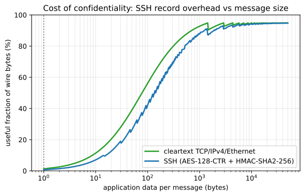
Useful fraction of wire bytes against message size, for SSH records versus cleartext, both over TCP/IPv4/Ethernet with the 38 bytes of framing from Problem 19.2. The 32-byte MAC plus block padding costs 14 percentage points at 64-byte messages and is invisible at 32 kB. The sawtooth is the block-padding quantisation; the drop past 1460 bytes is the second TCP segment.
A keystroke costs 142 wire bytes against cleartext’s 79, an efficiency of 0.70%, and the 78 bytes of framing from Problem 19.2 already dominate before any cryptography exists. A 32 kB record runs at 94.63% against cleartext’s 94.81%, so confidentiality is nearly free for bulk transfer and nearly all cost for typing. Setup takes about 9 round trips against TCP’s 1 – roughly 0.9 s at a 100 ms RTT before the shell prompt – though a real implementation pipelines some, so treat 5 to 9 as the range.
Is it fair that my neighbor’s iPad downloads faster?
Problem 20.1 — Fairness–efficiency unification
Fairness–efficiency unification. The definition of the fairness measure was given in Section 20.2.1 as follows:
\begin{equation*} f_\beta(\mathbf{x}) = \begin{cases} \operatorname{sign}(1-\beta)\left(\sum_{i=1}^{n}\left(\dfrac{x_i}{w(\mathbf{x})}\right)^{1-\beta}\right)^{1/\beta}, & \text{if } \beta \neq 0,\\[2ex] \exp\left(-\sum_{i=1}^{n}\dfrac{x_i}{w(\mathbf{x})}\log\dfrac{x_i}{w(\mathbf{x})}\right), & \text{if } \beta = 0, \end{cases} \end{equation*}
where \(w(\mathbf{x}) = \sum_{j=1}^{n} x_j\).
(a) Prove that indeed \(\lim_{\beta\to 0} f_\beta(\mathbf{x}) = f_0(\mathbf{x})\).
(b) Consider two allocation vectors \(\mathbf{x} = [0.1\; 0.2\; 0.3\; 0.6]\), \(\mathbf{y} = [0.2\; 0.2\; 0.8\; 0.9]\). Plot \(f_\beta(\mathbf{x})\) and \(f_\beta(\mathbf{y})\) as functions of \(-10 \le \beta \le 10\) on the same graph.
(c) Fix \(\beta = 0.5\). Plot the fairness–efficiency measures \(F_{\beta,\lambda}(\mathbf{x})\) and \(F_{\beta,\lambda}(\mathbf{y})\) as functions of \(0 \le \frac{1}{\lambda} \le 1\), on the same graph. (difficulty: \(\star\star\))
(a) The \(\beta \to 0\) limit is \(e^{H(\mathbf{p})}\); (b) the ranking swaps twice, at \(\beta \approx -0.975\) and \(\beta \approx 5.92\); (c) the curves cross at \(1/\lambda = 0.0282\).
(a) Put \(p_i = x_i/w(\mathbf{x})\), so \(\sum_i p_i = 1\) and, by the Axiom of Homogeneity, \(f_\beta\) sees \(\mathbf{x}\) only through \(\mathbf{p}\). For \(|\beta| < 1\) the prefactor \(\operatorname{sign}(1-\beta)\) is \(+1\), so \(f_\beta = S(\beta)^{1/\beta}\) with \(S(\beta) = \sum_i p_i^{1-\beta}\). Each \(p_i^{1-\beta} = e^{(1-\beta)\log p_i}\) is smooth, so
\begin{equation*} S(0) = 1, \qquad S’(\beta) = -\sum_i p_i^{1-\beta}\log p_i, \qquad S’(0) = H(\mathbf{p}), \end{equation*}
the entropy of Table 20.1. Since \(\log S(0) = 0\), L’Hopital on \(\log f_\beta = \log S(\beta)/\beta\) gives
\begin{equation*} \lim_{\beta\to0}\log f_\beta(\mathbf{x}) = \frac{S’(0)}{S(0)} = H(\mathbf{p}), \qquad \lim_{\beta\to0} f_\beta(\mathbf{x}) = e^{H(\mathbf{p})} = f_0(\mathbf{x}), \end{equation*}
exponentiating by continuity. The limit is two-sided, nothing above using the sign of \(\beta\). If some \(p_i = 0\), the exponent \(1-\beta\) is positive so that term drops from \(S(\beta)\), and \(0\log0 = 0\) drops it from \(H(\mathbf{p})\), so the argument runs verbatim on the support.
import numpy as np
def f(beta, x):
p = np.asarray(x, float); p = p / p.sum()
if abs(beta) < 1e-12:
return np.exp(-(p * np.log(p)).sum())
return np.sign(1 - beta) * (np.power(p, 1 - beta).sum())**(1 / beta)
x = np.array([0.1, 0.2, 0.3, 0.6])
y = np.array([0.2, 0.2, 0.8, 0.9])
for b in [1e-1, 1e-2, 1e-3, 1e-4, 1e-5]:
print(f"beta={b:8.0e} f_beta(x)={f(b,x):.10f} f_beta(y)={f(b,y):.10f}")
print(f"beta=0 f_0(x)={f(0,x):.10f} f_0(y)={f(0,y):.10f}")
beta= 1e-01 f_beta(x)=3.3728187314 f_beta(y)=3.3050755033
beta= 1e-02 f_beta(x)=3.3218343489 f_beta(y)=3.2553352600
beta= 1e-03 f_beta(x)=3.3168511129 f_beta(y)=3.2505420392
beta= 1e-04 f_beta(x)=3.3163539336 f_beta(y)=3.2500644956
beta= 1e-05 f_beta(x)=3.3163042270 f_beta(y)=3.2500167589
beta=0 f_0(x)=3.3162987043 f_0(y)=3.2500114551
Convergence is first order in \(\beta\), as \(\log S(\beta) = \beta H + O(\beta^2)\) predicts.
(b) The normalized vectors are
\begin{equation*} \frac{\mathbf{x}}{1.2} = \left[\tfrac{1}{12}\;\; \tfrac{1}{6}\;\; \tfrac{1}{4}\;\; \tfrac{1}{2}\right], \qquad \frac{\mathbf{y}}{2.1} = \left[\tfrac{2}{21}\;\; \tfrac{2}{21}\;\; \tfrac{8}{21}\;\; \tfrac{9}{21}\right], \end{equation*}
and neither majorizes the other in the sense of (20.2) – the ascending partial sums \((0.083, 0.250, 0.500, 1)\) and \((0.095, 0.190, 0.571, 1)\) cross. Since \(f_\beta\) is Schur-concave, majorization would have fixed one ordering for every \(\beta\); without it the ordering may depend on \(\beta\), and it does.
import numpy as np
import matplotlib.pyplot as plt
from scipy.optimize import brentq
bs = np.linspace(-10, 10, 4001)
bs = bs[np.abs(bs) > 1e-9]
fx = np.array([f(b, x) for b in bs])
fy = np.array([f(b, y) for b in bs])
plt.figure(figsize=(7, 4.5))
for m in [bs < 1, bs > 1]:
plt.plot(bs[m], fx[m], 'C0-', lw=1.8, label=r'$f_\beta(x)$' if m[0] else None)
plt.plot(bs[m], fy[m], 'C3--', lw=1.8, label=r'$f_\beta(y)$' if m[0] else None)
plt.axvline(1, color='0.6', ls=':'); plt.axhline(0, color='0.8', lw=0.8)
plt.ylim(-11, 5); plt.xlabel(r'$\beta$'); plt.ylabel(r'fairness $f_\beta$')
plt.title(r'$x=[0.1,0.2,0.3,0.6]$ vs $y=[0.2,0.2,0.8,0.9]$')
plt.legend(); plt.grid(alpha=.3)
plt.savefig('nl-ch20-fbeta-xy.svg', dpi=150, bbox_inches='tight')
for b in [-10, -5, -2, -1, -0.5, 0, 0.5, 0.9, 1.1, 2, 5, 10]:
who = 'x more fair' if f(b, x) > f(b, y) else 'y more fair'
print(f"{b:6.1f} {f(b,x):12.6f} {f(b,y):12.6f} {who}")
d = lambda b: f(b, x) - f(b, y)
print("crossover 1:", brentq(d, -1.0, -0.5))
print("crossover 2:", brentq(d, 5.0, 10.0))
-10.0 2.143441 2.478944 y more fair
-5.0 2.289656 2.551117 y more fair
-2.0 2.618615 2.714322 y more fair
-1.0 2.880000 2.882353 y more fair
-0.5 3.070851 3.030084 x more fair
0.0 3.316299 3.250011 x more fair
0.5 3.625331 3.568625 x more fair
0.9 3.920076 3.905008 x more fair
1.1 -4.082221 -4.098895 x more fair
2.0 -4.898979 -5.094932 x more fair
5.0 -7.407583 -7.541063 x more fair
10.0 -9.361600 -8.895564 y more fair
crossover 1: -0.9749491452020058
crossover 2: 5.920393074711568
![Fairness \(f_\beta\) of \(x=[0.1,0.2,0.3,0.6]\) (solid) and \(y=[0.2,0.2,0.8,0.9]\) (dashed) over \(-10\le\beta\le10\). The curves jump from \(+\infty\) to \(-\infty\) across \(\beta=1\) because of the \(\operatorname{sign}(1-\beta)\) prefactor. The two vectors swap fairness ranking twice, near \(\beta=-0.975\) and near \(\beta=5.92\).](/words/library/books/nl-ch20-fbeta-xy.svg)
Fairness \(f_\beta\) of \(x=[0.1,0.2,0.3,0.6]\) (solid) and \(y=[0.2,0.2,0.8,0.9]\) (dashed) over \(-10\le\beta\le10\). The curves jump from \(+\infty\) to \(-\infty\) across \(\beta=1\) because of the \(\operatorname{sign}(1-\beta)\) prefactor. The two vectors swap fairness ranking twice, near \(\beta=-0.975\) and near \(\beta=5.92\).
Reading the plot: the discontinuity at \(\beta = 1\) is the \(\operatorname{sign}(1-\beta)\) factor, both curves running to \(+\infty\) as \(\beta \uparrow 1\) and returning from \(-\infty\). At \(\beta = -1\) the values are \(nJ\) for Jain’s index (2.880 against 2.882) and at \(\beta = 0\) they are \(e^H\) (3.316 against 3.250). As \(\beta \to -\infty\), \(f_\beta \to w/\max_i x_i\), namely 2 and \(2.\overline{3}\), so \(\mathbf{y}\) wins where only the largest share counts; as \(\beta \to +\infty\), \(f_\beta \to -w/\min_i x_i\), namely \(-12\) and \(-10.5\), so \(\mathbf{y}\) wins again where only the worst-off counts. Across the middle band \(-0.975 < \beta < 5.92\), which holds entropy, Jain’s index and proportional fairness, \(\mathbf{x}\) is fairer.
(c) Equation (20.6) drops the Axiom of Homogeneity and gives
\begin{equation*} F_{\beta,\lambda}(\mathbf{x}) \;=\; f_\beta(\mathbf{x})\cdot\Big(\sum_i x_i\Big)^{1/\lambda}, \end{equation*}
with \(1/\lambda\) the degree of homogeneity: \(1/\lambda = 0\) recovers pure fairness, larger values weight the total resource. At \(\beta = 0.5\), \(f_{0.5}(\mathbf{x}) = \bigl(\sum_i\sqrt{x_i/w(\mathbf{x})}\bigr)^2\), with \(w(\mathbf{x}) = 1.2\) and \(w(\mathbf{y}) = 2.1\).
import numpy as np
import matplotlib.pyplot as plt
from scipy.optimize import brentq
beta = 0.5
t = np.linspace(0, 1, 401) # t = 1/lambda
Fx = f(beta, x) * np.power(x.sum(), t)
Fy = f(beta, y) * np.power(y.sum(), t)
plt.figure(figsize=(7, 4.5))
plt.plot(t, Fx, 'C0-', lw=1.8, label=r'$F_{0.5,\lambda}(x)$, $\sum x_i=1.2$')
plt.plot(t, Fy, 'C3--', lw=1.8, label=r'$F_{0.5,\lambda}(y)$, $\sum y_i=2.1$')
g = lambda s: f(beta, x) * x.sum()**s - f(beta, y) * y.sum()**s
xc = brentq(g, 0, 1)
plt.plot([xc], [f(beta, x) * x.sum()**xc], 'ko', ms=5)
plt.annotate(f'crossover $1/\\lambda={xc:.4f}$', (xc, f(beta, x) * x.sum()**xc),
textcoords='offset points', xytext=(12, -14))
plt.xlabel(r'degree of homogeneity $1/\lambda$'); plt.ylabel(r'$F_{\beta,\lambda}$')
plt.title(r'fairness-efficiency measure, $\beta=0.5$')
plt.legend(); plt.grid(alpha=.3)
plt.savefig('nl-ch20-Fbetalambda-xy.svg', dpi=150, bbox_inches='tight')
print(f"f_0.5(x)={f(beta,x):.6f} f_0.5(y)={f(beta,y):.6f}")
print(f"1/lambda=0 : F(x)={f(beta,x):.6f} F(y)={f(beta,y):.6f}")
print(f"1/lambda=1 : F(x)={f(beta,x)*1.2:.6f} F(y)={f(beta,y)*2.1:.6f}")
print(f"crossover at 1/lambda = {xc:.6f} "
f"(closed form {np.log(f(beta,x)/f(beta,y))/np.log(2.1/1.2):.6f})")
f_0.5(x)=3.625331 f_0.5(y)=3.568625
1/lambda=0 : F(x)=3.625331 F(y)=3.568625
1/lambda=1 : F(x)=4.350397 F(y)=7.494113
crossover at 1/lambda = 0.028172 (closed form 0.028172)
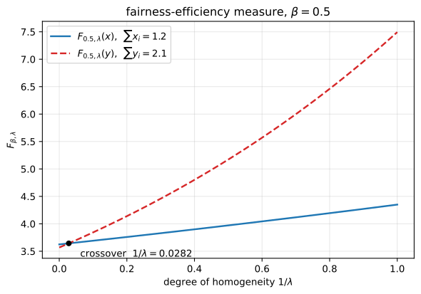
Fairness–efficiency measure \(F_{\beta,\lambda}=f_\beta\cdot(\sum_i x_i)^{1/\lambda}\) at \(\beta=0.5\), plotted against the degree of homogeneity \(1/\lambda\). At \(1/\lambda=0\) only the distribution counts and \(x\) edges ahead; the curves cross at \(1/\lambda\approx0.0282\) and thereafter the larger total resource of \(y\) dominates.
Since \(F_{\beta,\lambda} = f_\beta \cdot w^{1/\lambda}\), both curves are exponentials in \(1/\lambda\) and cross exactly once, at
\begin{equation*} \frac{1}{\lambda^\star} \;=\; \frac{\log\big(f_\beta(\mathbf{x})/f_\beta(\mathbf{y})\big)}{\log\big(w(\mathbf{y})/w(\mathbf{x})\big)} \;=\; \frac{\log(3.625331/3.568625)}{\log(2.1/1.2)} \;=\; 0.0282 . \end{equation*}
At \(\beta = 0.5\), \(\mathbf{x}\) is fairer by only \(1.6\%\) while \(\mathbf{y}\) carries \(75\%\) more resource, so any weight on efficiency beyond \(1/\lambda = 0.028\) reverses the verdict.
Problem 20.2 — Reverse-engineering β
Reverse-engineering \(\beta\). Different values of the parameter \(\beta\) lead to different fairness functions. A natural question, then, is how to determine \(\beta\). This problem will explore one way to do that.
Consider the following scenario: there are three people who want bandwidth on a shared link, and you have 10 Mbps to allocate to them. Assume each is equally deserving of the bandwidth. There are four possible allocations: \((5,\,2.5,\,2.5)\), \((4.5,\,3.5,\,2)\), \((6,\,2,\,2)\), and \((4.5,\,4.5,\,1)\).
We will now walk through the process of determining a possible \(\beta\) value. Suppose that there are three possibilities: \(\beta = -10\), or \(0.5\), or \(2\). For parts (a) and (b), choose the more fair allocation of the two options provided, and then find which values of \(\beta\) can be eliminated given your answer.
(a) \((5,\,2.5,\,2.5)\) and \((4.5,\,3.5,\,2)\).
(b) \((6,\,2,\,2)\) and \((4.5,\,4.5,\,1)\).
(c) How many values of \(\beta\) are compatible with both of your answers in (a) and (b)?
(d) Suppose you chose \((5,\,2.5,\,2.5)\) in part (a) and \((4.5,\,4.5,\,1)\) in part (b) as the most fair allocations. How many values of \(\beta\) are compatible with both answers? Can you intuitively explain why? What does this tell you about quantitative modeling of fairness? (difficulty: \(\star\star\))
Choosing \(A = (5,2.5,2.5)\) and \(C = (6,2,2)\) leaves exactly one compatible \(\beta\), namely 2; the pair \(A\), \(D\) leaves none.
Write \(A=(5,2.5,2.5)\), \(B=(4.5,3.5,2)\), \(C=(6,2,2)\), \(D=(4.5,4.5,1)\). All four have \(w = 10\), so (20.1) compares distributions only. For \(\beta > 1\) the prefactor \(\operatorname{sign}(1-\beta)\) is negative, so larger (less negative) \(f_\beta\) still means fairer. Evaluating (20.1) at the three candidate \(\beta\):
import numpy as np
def f(beta, x):
p = np.asarray(x, float); p = p / p.sum()
if abs(beta) < 1e-12:
return np.exp(-(p * np.log(p)).sum())
return np.sign(1 - beta) * (np.power(p, 1 - beta).sum())**(1 / beta)
alloc = {'A=(5,2.5,2.5)': [5, 2.5, 2.5], 'B=(4.5,3.5,2)': [4.5, 3.5, 2],
'C=(6,2,2)': [6, 2, 2], 'D=(4.5,4.5,1)': [4.5, 4.5, 1]}
betas = [-10, 0.5, 2]
print(f"{'allocation':16s}" + "".join(f" beta={b:<6}" for b in betas))
for k, v in alloc.items():
print(f"{k:16s}" + "".join(f" {f(b,v):11.6f}" for b in betas))
print()
for b in betas:
a = 'A' if f(b, alloc['A=(5,2.5,2.5)']) > f(b, alloc['B=(4.5,3.5,2)']) else 'B'
c = 'C' if f(b, alloc['C=(6,2,2)']) > f(b, alloc['D=(4.5,4.5,1)']) else 'D'
print(f"beta={b:6}: (a) A vs B -> {a} | (b) C vs D -> {c}")
allocation beta=-10 beta=0.5 beta=2
A=(5,2.5,2.5) 2.143338 2.914214 -3.162278
B=(4.5,3.5,2) 2.392253 2.922876 -3.174802
C=(6,2,2) 1.754014 2.785641 -3.415650
D=(4.5,4.5,1) 2.245759 2.748528 -3.800585
beta= -10: (a) A vs B -> B | (b) C vs D -> D
beta= 0.5: (a) A vs B -> B | (b) C vs D -> C
beta= 2: (a) A vs B -> A | (b) C vs D -> C
(a) Neither vector majorizes the other – the ascending partial sums (20.2) are \((2.5, 5, 10)\) for \(A\) and \((2, 5.5, 10)\) for \(B\), and they cross – so Schur-concavity leaves the answer to \(\beta\). I choose \(A\), on Rawls’ difference principle (Section 20.4.1): \(B\) buys a flatter middle by cutting the worst-off user \(20\%\), from 2.5 to 2 Mbps, while the best-off gives up only 0.5. Since \(f_2(A) = -3.1623 > f_2(B) = -3.1748\) but the ordering reverses at \(\beta = -10\) and \(\beta = 0.5\), this keeps only \(\beta = 2\). (Choosing \(B\) instead would keep \(\{-10, 0.5\}\).)
(b) Again majorization-incomparable: \((2, 4, 10)\) against \((1, 5.5, 10)\). I choose \(C\), for the same reason – \(D\) halves the worst-off user’s rate to compress the top two – which keeps \(\{0.5, 2\}\). Only \(\beta = -10\) disagrees, because as \(\beta \to -\infty\) the measure becomes the min ratio \(w/\max_i x_i\) of Table 20.1, \(10/6 = 1.67\) against \(10/4.5 = 2.22\): a strongly negative \(\beta\) caps the rich and is blind to the user on 1 Mbps.
(c) The surviving set is \(\{2\} \cap \{0.5,2\} = \{2\}\), so exactly one value survives. The four possible answer pairs:
| answers | surviving \(\beta\) | count |
|---|---|---|
| \(A\), \(C\) | \(\{2\}\) | 1 |
| \(B\), \(C\) | \(\{0.5\}\) | 1 |
| \(B\), \(D\) | \(\{-10\}\) | 1 |
| \(A\), \(D\) | \(\varnothing\) | 0 |
(d) Zero values are compatible: \(A\) over \(B\) requires \(\beta = 2\) and \(D\) over \(C\) requires \(\beta = -10\). This is not an artifact of the three candidates – sweeping the whole real line, the two preferences never hold together.
import numpy as np
import matplotlib.pyplot as plt
from scipy.optimize import brentq
A, B = [5, 2.5, 2.5], [4.5, 3.5, 2]
C, D = [6, 2, 2], [4.5, 4.5, 1]
bAB = brentq(lambda b: f(b, A) - f(b, B), 1.2, 2.0)
bDC = brentq(lambda b: f(b, D) - f(b, C), -1.0, 0.5)
print(f"A preferred to B iff beta > {bAB:.6f}")
print(f"D preferred to C iff beta < {bDC:.6f}")
bs = np.linspace(-10, 10, 4001)
bs = bs[(np.abs(bs - 1) > 1e-3) & (np.abs(bs) > 1e-9)]
plt.figure(figsize=(7, 4.5))
for m in [bs < 1, bs > 1]:
plt.plot(bs[m], [f(b, A) - f(b, B) for b in bs[m]], 'C0-', lw=1.8,
label=r'$f_\beta(A)-f_\beta(B)$' if m[0] else None)
plt.plot(bs[m], [f(b, D) - f(b, C) for b in bs[m]], 'C3--', lw=1.8,
label=r'$f_\beta(D)-f_\beta(C)$' if m[0] else None)
plt.axhline(0, color='k', lw=.8); plt.axvline(1, color='.6', ls=':')
plt.axvspan(bAB, 10, color='C0', alpha=.10)
plt.axvspan(-10, bDC, color='C3', alpha=.10)
for b in [-10, 0.5, 2]:
plt.axvline(b, color='k', ls='-.', lw=.8, alpha=.5)
plt.ylim(-0.6, 0.6); plt.xlabel(r'$\beta$'); plt.ylabel('fairness difference')
plt.title(r'"A over B" needs $\beta>1.394$; "D over C" needs $\beta<-0.031$')
plt.legend(loc='lower right'); plt.grid(alpha=.3)
plt.savefig('nl-ch20-reverse-engineer-beta.svg', dpi=150, bbox_inches='tight')
print("the two admissible ranges are disjoint:", bAB > bDC)
A preferred to B iff beta > 1.394295
D preferred to C iff beta < -0.030833
the two admissible ranges are disjoint: True
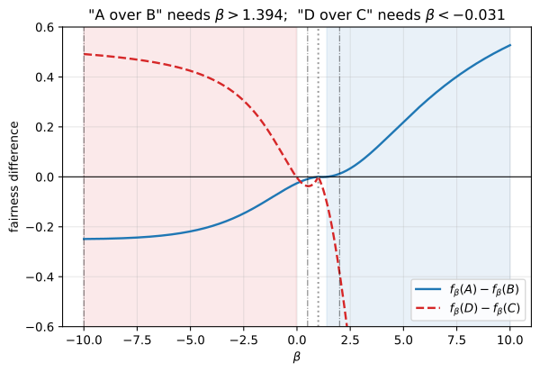
Fairness differences as functions of \(\beta\). Judging \(A=(5,2.5,2.5)\) fairer than \(B=(4.5,3.5,2)\) requires \(\beta>1.394\) (blue band); judging \(D=(4.5,4.5,1)\) fairer than \(C=(6,2,2)\) requires \(\beta<-0.031\) (red band). The bands do not overlap, so no \(\beta\) at all rationalizes both answers.
Sorted, the two moves are the same trade – cut the bottom, fatten the middle, shave the top:
\begin{equation*} A=(2.5,\,2.5,\,5) \to B=(2,\,3.5,\,4.5), \qquad C=(2,\,2,\,6) \to D=(1,\,4.5,\,4.5). \end{equation*}
Preferring \(A\) rejects that trade, weighting the worst-off user heavily as large \(\beta\) does; preferring \(D\) accepts it in a harsher form, the bottom user losing half her rate rather than a fifth. No single monotone preference along the bottom-versus-top axis, which is all the one-parameter family traces out, can do both. The empty set is the model detecting an inconsistency in the answers rather than failing: each binary question is a halfspace constraint on \(\beta\), so elicitation is cheap, and when it returns nothing the honest options are to revise a judgment or to accept that one scalar is too coarse – which is the door (20.6) opens with user weights \(\{q_i\}\) and the efficiency weight \(\lambda\).
Problem 20.3 — Multi-resource fairness
Multi-resource fairness. Recall that the fairness–efficiency functions introduced in the lecture notes have the form
\begin{equation*} F_{\beta,\lambda}(\mathbf{x}) = \operatorname{sign}(1-\beta)\left(\sum_{i=1}^{n}\left(\frac{x_i}{\sum_{j=1}^n x_j}\right)^{1-\beta}\right)^{1/\beta}\left(\sum_{i=1}^{n} x_i\right)^{\lambda}, \tag{20.10} \end{equation*}
where \(\mathbf{x}\) is an \(n\)-dimensional resource allocation vector. But, in some contexts, the allocation of one resource is not enough. For instance, consider a data center utilized by two users. Each user runs one type of job, and the two types of jobs have different resource needs. Both require memory and CPU (processing power), but user A’s jobs require 1 GB of memory and 2 MIPS (a unit of computational power) of CPUs per job, while user B’s jobs require 2 GB of memory and 1.5 MIPS CPUs per job. These resources are limited: there are 8 GB of available memory and 12 MIPS of CPUs. Clearly, just allocating memory or just allocating CPUs is not enough: we need to consider the fairness of both resource allocations.
This homework question explores two different ways of measuring the fairness of multi-resource allocations, as in the above example about data centers. First, one could just measure the fairness of the number of jobs allocated to each user. Each user is allocated enough resources to complete this number of jobs. For instance, if user A is allocated 2 jobs, she receives 2 GB of memory and 4 MIPS of CPUs. The resource allocation vector in (20.10) is just the number of jobs assigned to each user. For instance, if user A is assigned 2 jobs and user B 3 jobs, the fairness of this allocation is
\begin{equation*} \operatorname{sign}(1-\beta)\left(\left(\frac{2}{2+3}\right)^{1-\beta}+\left(\frac{3}{2+3}\right)^{1-\beta}\right)^{1/\beta}(2+3)^{\lambda}. \end{equation*}
But this approach misses the heterogeneity of the resource requests among the users. The second way of measuring multi-resource fairness involves dominant shares. These are defined as the maximum fraction of each resource received by the user. For instance, if user A gets 2 jobs, she receives 2 GB of memory and 4 MIPS of CPUs. Then A receives 1/4 of the available memory but 1/3 of the CPUs. User A’s dominant resource is CPUs, and her dominant share is 1/3. These dominant shares are then taken as the resource allocation vector. For example, if user A’s dominant share is 1/3 and user B’s is 2/3, the allocation vector \(\mathbf{x}\) in (20.10) is \([1/3\;\; 2/3]\).
(a) What is user B’s dominant resource? Calculate the dominant shares for users A and B in terms of \(x_A\) and \(x_B\), the number of jobs allocated to users A and B, respectively.
(b) Formulate the maximization problem for multi-resource fairness in the datacenter example above, using both fairness on jobs and fairness on dominant shares (i.e., write down two formulations, one for fairness on jobs and one for fairness on dominant shares). Use your answers to part (a) and (20.10) to write down the objective function for maximizing fairness on dominant shares.
(c) Numerically solve for the optimal resource allocation according to your formulations in part (b), with the resource requirements given above and \(\beta = 0.5\) and \(\lambda = 1\). (Non-integer numbers of jobs are allowed.) Are the optimal allocations the same? Which do you think is more “fair”? (difficulty: \(\star\star\star\))
(a) A is CPU-bound with \(s_A = x_A/6\), B memory-bound with \(s_B = x_B/4\); (b) the two programs below; (c) \((4.8, 1.6)\) versus \((32/7, 12/7)\), and the dominant-share answer is the fairer one.
(a) User A’s \(x_A\) jobs take fractions \(x_A/8\) of memory and \(2x_A/12 = x_A/6\) of CPU, so CPU dominates and \(s_A = x_A/6\); user B’s take \(2x_B/8 = x_B/4\) of memory against \(1.5x_B/12 = x_B/8\) of CPU, so memory dominates and \(s_B = x_B/4\). The dominant resources differ, which is exactly when the two fairness notions diverge.
(b) The feasible set is physical and common to both.
\begin{equation*} \mathcal{C} = \Big\{(x_A,x_B) \;:\; \underbrace{x_A + 2x_B \le 8}_{\text{memory}},\;\; \underbrace{2x_A + 1.5 x_B \le 12}_{\text{CPU}},\;\; x_A \ge 0,\; x_B \ge 0 \Big\}. \end{equation*}
Formulation 1, fairness on jobs. Put \(\mathbf{x} = [x_A\;\; x_B]\) into (20.10):
\begin{equation*} \begin{array}{ll} \text{maximize} & \operatorname{sign}(1-\beta)\left[\left(\dfrac{x_A}{x_A+x_B}\right)^{1-\beta}+\left(\dfrac{x_B}{x_A+x_B}\right)^{1-\beta}\right]^{1/\beta}\big(x_A+x_B\big)^{\lambda}\\[2ex] \text{subject to} & x_A + 2x_B \le 8, \qquad 2x_A + 1.5x_B \le 12\\[0.5ex] \text{variables} & x_A \ge 0,\ x_B \ge 0 . \end{array} \end{equation*}
Formulation 2, fairness on dominant shares. Put \(\mathbf{s} = [\,s_A\;\; s_B\,] = [\,x_A/6\;\;\; x_B/4\,]\) into (20.10). With \(\sigma := s_A + s_B = \dfrac{x_A}{6}+\dfrac{x_B}{4} = \dfrac{2x_A + 3x_B}{12}\),
\begin{equation*} \begin{array}{ll} \text{maximize} & \operatorname{sign}(1-\beta)\left[\left(\dfrac{x_A/6}{\sigma}\right)^{1-\beta}+\left(\dfrac{x_B/4}{\sigma}\right)^{1-\beta}\right]^{1/\beta}\left(\dfrac{2x_A+3x_B}{12}\right)^{\lambda}\\[2ex] \text{subject to} & x_A + 2x_B \le 8, \qquad 2x_A + 1.5x_B \le 12\\[0.5ex] \text{variables} & x_A \ge 0,\ x_B \ge 0 . \end{array} \end{equation*}
Only the objective changes; the efficiency factor becomes total jobs in the first and total dominant share in the second. At \(\beta = 0.5\), \(\lambda = 1\), for any \(\mathbf{v}\) with \(V = \sum_i v_i\),
\begin{equation*} F_{0.5,1}(\mathbf{v}) = \left[\sum_i \left(\frac{v_i}{V}\right)^{1/2}\right]^{2} V = \frac{\big(\sum_i \sqrt{v_i}\big)^2}{V}\cdot V = \Big(\sum_i \sqrt{v_i}\Big)^{2}. \end{equation*}
So the two objectives collapse to
\begin{equation*} \text{jobs:}\quad \big(\sqrt{x_A}+\sqrt{x_B}\big)^2, \qquad\qquad \text{dominant shares:}\quad \Big(\sqrt{x_A/6}+\sqrt{x_B/4}\Big)^2 , \end{equation*}
both concave, so each is a concave maximization over a polytope with a unique optimum. Note \(\lambda = 1\) is exactly the Pareto-preserving threshold \(\bar\lambda = \beta/(1-\beta)\) of (20.5) at \(\beta = 0.5\), so by the remark below (20.7) each formulation is \(\alpha\)-fair allocation with \(\alpha = 1/2\) – visible above, since maximizing \((\sum_i\sqrt{v_i})^2\) maximizes \(\sum_i \sqrt{v_i}\).
(c)
import numpy as np
from scipy.optimize import minimize
beta, lam = 0.5, 1.0
def F(v): # F_{beta,lambda} of equation (20.10)
v = np.asarray(v, float)
if (v <= 0).any():
return 0.0
p = v / v.sum()
return np.sign(1 - beta) * (np.power(p, 1 - beta).sum())**(1 / beta) * v.sum()**lam
cons = [{'type': 'ineq', 'fun': lambda z: 8 - (z[0] + 2.0 * z[1])}, # memory
{'type': 'ineq', 'fun': lambda z: 12 - (2.0 * z[0] + 1.5 * z[1])}] # CPU
bnds = [(1e-9, None), (1e-9, None)]
def solve(obj, label):
best = None
for g in [(1, 1), (4, 1), (1, 3), (4.8, 1.6), (3, 2), (0.5, 3.5), (5.5, 0.2)]:
r = minimize(lambda z: -obj(z), g, constraints=cons, bounds=bnds,
method='SLSQP', options={'maxiter': 2000, 'ftol': 1e-14})
if r.success and (best is None or -r.fun > -best.fun):
best = r
z = best.x
print(f"{label}: xA={z[0]:.6f} xB={z[1]:.6f} objective={-best.fun:.6f}")
print(f" memory used {z[0]+2*z[1]:.4f}/8 cpu used {2*z[0]+1.5*z[1]:.4f}/12")
print(f" dominant shares: sA=xA/6={z[0]/6:.6f} sB=xB/4={z[1]/4:.6f}")
print(f" F_jobs={F(z):.6f} F_domshare={F([z[0]/6, z[1]/4]):.6f}")
return z
zj = solve(F, "fairness on JOBS ")
zd = solve(lambda z: F([z[0]/6, z[1]/4]), "fairness on DOM. SHARES ")
fairness on JOBS : xA=4.800000 xB=1.600000 objective=11.942563
memory used 8.0000/8 cpu used 12.0000/12
dominant shares: sA=xA/6=0.800000 sB=xB/4=0.400000
F_jobs=11.942563 F_domshare=2.331371
fairness on DOM. SHARES : xA=4.571429 xB=1.714286 objective=2.333333
memory used 8.0000/8 cpu used 11.7143/12
dominant shares: sA=xA/6=0.761905 sB=xB/4=0.428571
F_jobs=11.884548 F_domshare=2.333333
The allocations differ. Fairness on jobs gives the vertex \((4.8, 1.6)\) where both constraints bind, value \((32+16\sqrt3)/5 = 11.9426\); fairness on dominant shares gives \((32/7, 12/7)\) on the memory face, leaving 0.286 MIPS idle, value \(49/21 = 7/3\) exactly.
By hand: maximizing \(\sqrt{x_A}+\sqrt{x_B}\) on the memory face \(x_A = 8-2x_B\) needs \(\sqrt{x_A} = 2\sqrt{x_B}\), giving \((16/3, 4/3)\), which violates CPU, and on the CPU face it needs \(\sqrt{x_A} = 0.75\sqrt{x_B}\), giving \((2.571, 4.571)\), which violates memory – so the optimum is the vertex. Maximizing \(\sqrt{x_A/6}+\sqrt{x_B/4}\) on the memory face needs \(x_A = \tfrac83 x_B\), giving \((32/7, 12/7)\) with CPU usage \(82/7 \le 12\) (Check!), a genuine face optimum.
import numpy as np
import matplotlib.pyplot as plt
zj = np.array([4.8, 1.6]); zd = np.array([32/7, 12/7]); zdrf = np.array([24/7, 16/7])
for nm, z in [("jobs-fair ", zj), ("dom-share-fair ", zd), ("equal dom share ", zdrf)]:
print(f"{nm} xA={z[0]:.6f} xB={z[1]:.6f} mem={z[0]+2*z[1]:.4f}/8 cpu={2*z[0]+1.5*z[1]:.4f}/12 "
f" sA={z[0]/6:.6f} sB={z[1]/4:.6f} "
f" Fjobs={(np.sqrt(z[0])+np.sqrt(z[1]))**2:.6f} Fds={(np.sqrt(z[0]/6)+np.sqrt(z[1]/4))**2:.6f}")
print("exact jobs opt value (32+16*sqrt3)/5 =", (32 + 16*np.sqrt(3))/5)
print("exact dom-share opt value 7/3 =", 7/3)
xa = np.linspace(0, 7.6, 400); xb = np.linspace(0, 4.5, 400)
XA, XB = np.meshgrid(xa, xb)
feas = (XA + 2*XB <= 8) & (2*XA + 1.5*XB <= 12)
plt.figure(figsize=(6.6, 5))
plt.contourf(XA, XB, np.where(feas, 1, np.nan), levels=[0, 2], colors=['#dfe8f5'])
Oj = (np.sqrt(XA) + np.sqrt(XB))**2
Od = (np.sqrt(XA/6) + np.sqrt(XB/4))**2
plt.contour(XA, XB, np.where(feas, Oj, np.nan), levels=np.linspace(6, 11.94, 7),
colors='C0', linewidths=.7, alpha=.8)
plt.contour(XA, XB, np.where(feas, Od, np.nan), levels=np.linspace(1.2, 2.3333, 7),
colors='C3', linewidths=.7, linestyles='--', alpha=.8)
b = np.linspace(0, 8, 200)
plt.plot(8 - 2*b, b, 'k-', lw=1.4); plt.plot(6 - 0.75*b, b, 'k-', lw=1.4)
plt.plot(*zj, 'C0o', ms=9)
plt.annotate('jobs-fair (4.800, 1.600)', zj, textcoords='offset points', xytext=(8, -18), color='C0')
plt.plot(*zd, 'C3s', ms=9)
plt.annotate('dominant-share-fair (4.571, 1.714)', zd, textcoords='offset points', xytext=(-70, 16), color='C3')
plt.plot(*zdrf, 'k^', ms=8)
plt.annotate('equal dominant shares (3.429, 2.286)', zdrf, textcoords='offset points', xytext=(-95, 14))
plt.xlim(0, 7.6); plt.ylim(0, 4.5)
plt.xlabel(r'$x_A$ (jobs to A)'); plt.ylabel(r'$x_B$ (jobs to B)')
plt.title(r'$\beta=0.5,\ \lambda=1$: two notions of multi-resource fairness')
plt.grid(alpha=.25)
plt.savefig('nl-ch20-multiresource.svg', dpi=150, bbox_inches='tight')
jobs-fair xA=4.800000 xB=1.600000 mem=8.0000/8 cpu=12.0000/12 sA=0.800000 sB=0.400000 Fjobs=11.942563 Fds=2.331371
dom-share-fair xA=4.571429 xB=1.714286 mem=8.0000/8 cpu=11.7143/12 sA=0.761905 sB=0.428571 Fjobs=11.884548 Fds=2.333333
equal dom share xA=3.428571 xB=2.285714 mem=8.0000/8 cpu=10.2857/12 sA=0.571429 sB=0.571429 Fjobs=11.313119 Fds=2.285714
exact jobs opt value (32+16*sqrt3)/5 = 11.942562584220408
exact dom-share opt value 7/3 = 2.3333333333333335
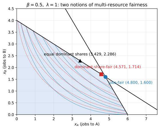
The feasible region (memory \(x_A+2x_B\le 8\) and CPU \(2x_A+1.5x_B\le 12\)) with level curves of the two objectives at \(\beta=0.5,\lambda=1\): solid blue for fairness on jobs, dashed red for fairness on dominant shares. The two optima are close but distinct; the triangle marks the equal-dominant-share (DRF) point that the \(\beta\to\infty\) limit would select.
The dominant-share formulation is the fairer one. The jobs metric takes a job as the unit of entitlement, but a job is not a comparable good across users – one of B’s eats twice the memory of one of A’s – so ranking by \([x_A\;\;x_B]\) embeds an exchange rate the data contradicts. Normalizing each user against her own bottleneck asks instead what fraction of the thing she needs she got, the only quantity here to which the Axiom of Homogeneity applies straight-facedly, and the metric under which sharing incentive, envy-freeness and strategy-proofness are provable.
The disagreement is small: at each optimum the other objective loses \(0.08\%\) and \(0.5\%\) respectively, and both points are Pareto optimal since memory binds at both. What moves the answer more is \(\beta\): at \(\beta = 0.5\) the dominant shares come out at \((0.762, 0.429)\), badly unequal, and not because efficiency overpowers fairness, since \(\lambda = \bar\lambda\) is already the most fairness-leaning Pareto-preserving setting. The strong notion is max-min on dominant shares, the \(\beta \to \infty\) limit of \(f_\beta\) alone at \(1/\lambda = 0\) (it cannot be reached at \(\lambda = 1\), since \(\bar\lambda < 0\) once \(\beta > 1\)). That gives \(s_A = s_B\), so \(x_A = 1.5x_B\) and memory binds at \(3.5x_B = 8\):
\begin{equation*} (x_A, x_B) = (24/7,\ 16/7), \qquad s_A = s_B = 4/7 , \end{equation*}
optimal since \(\min(s_A,s_B) \ge s\) forces \(x_A \ge 6s\), \(x_B \ge 4s\) and hence \(14s \le 8\). This is what a DRF scheduler implements, and it costs \(40/7 = 5.71\) jobs against the vertex’s 6.4, an \(11\%\) drop.
Problem 20.4 — Cake-cutting fairness
Cake-cutting fairness. Suppose each person has a valuation function that maps a given piece of a cake into a positive number. For example, if the cake has a chocolate half and a vanilla half, Alice may like the chocolate half twice as much as the vanilla half, while Bob is the other way round. “One cuts, the other selects” is a well-known procedure of dividing a cake between two people such that both value their own share to be at least half of the whole cake. Alice first cuts the cake into two pieces with each piece having the same value to her, and then Bob selects among the two pieces.
Can you come up with a procedure of dividing a cake for three participants so that they all value their own share to be at least one third of the whole cake?
(Hint: First divide the cake into three pieces whose values are equal for one participant.)
(More detail can be found in the following survey: S. J. Brams, M. A. Jones, and C. Klamler, “Better ways to cut a cake,” Notice of the American Mathematics Society, vol. 53, no. 11, pp. 1314–1321, December 2006.) (difficulty: \(\star\star\star\))
Steinhaus’ lone-divider procedure, below, gives every participant a share she values at \(\ge 1/3\).
Write \(v_i\) for participant \(i\)’s valuation, a non-negative atomless measure with \(v_i(\mathcal{K}) = 1\); atomlessness supplies the intermediate value property that any piece \(S\) has a sub-piece worth \(q\,v_i(S)\) for any \(q \in [0,1]\). Nobody knows anyone else’s \(v_i\).
Divide. Alice cuts \(\mathcal{K}\) into \(P_1, P_2, P_3\) with \(v_A(P_j) = 1/3\) each, which atomlessness permits.
Bid. Bob and Carol each privately name the set of pieces they consider acceptable, meaning worth at least \(1/3\) to them:
\begin{equation*} \mathcal{A}_B = \{ j : v_B(P_j) \ge 1/3 \}, \qquad \mathcal{A}_C = \{ j : v_C(P_j) \ge 1/3 \}. \end{equation*}
Neither set is empty: \(v_B(P_1)+v_B(P_2)+v_B(P_3) = 1\), so at least one piece must be worth \(\ge 1/3\) to Bob, and likewise for Carol.
Case 1 – the bids can be matched. Suppose there exist \(j \in \mathcal{A}_B\) and \(k \in \mathcal{A}_C\) with \(j \neq k\). Give \(P_j\) to Bob, \(P_k\) to Carol, and the remaining piece to Alice. Done.
Case 2 – the bids cannot be matched. By Hall’s marriage condition, a system of distinct representatives for two non-empty sets fails only if \(\mathcal{A}_B = \mathcal{A}_C = \{P_j\}\) for one common piece \(P_j\). Let \(P_m, P_n\) be the other two pieces. Give one of them, say \(P_m\), to Alice. Bob and Carol now run ordinary “one cuts, the other chooses” on the leftover \(R = P_j \cup P_n\): Bob cuts \(R\) into \(R_1, R_2\) with \(v_B(R_1) = v_B(R_2) = \tfrac12 v_B( R)\), and Carol takes whichever of \(R_1, R_2\) she values more.
Proportionality. Alice always receives some \(P_j\), worth exactly \(1/3\) to her. In Case 1 Bob receives a \(P_j \in \mathcal{A}_B\), worth \(\ge 1/3\) by definition, and likewise Carol. In Case 2, \(\mathcal{A}_B = \{P_j\}\) means \(v_B(P_m) < 1/3\), so
\begin{equation*} v_B( R) = 1 - v_B(P_m) > \tfrac23 , \end{equation*}
and Bob halves \(R\) by his own measure, so whichever half Carol leaves is worth \(\tfrac12 v_B( R) > \tfrac13\) to him; identically \(v_C( R) > 2/3\) and Carol’s chosen half is worth \(\ge \tfrac12 v_C( R) > \tfrac13\). \(\blacksquare\)
The load-bearing step is \(v_B(P_m) < 1/3 \Rightarrow v_B( R) > 2/3\): half of something worth more than \(2/3\) exceeds \(1/3\), which is what a two-person divide-and-choose on the leftover alone would not deliver. Each guarantee is also self-enforcing, derived from the acting participant’s own cuts and choices, so misreporting an acceptable set only risks a piece one values below \(1/3\) oneself. Note the naive iteration fails: if Alice halves the cake, Bob picks, and each then splits with Carol, nothing forces those halves to be worth \(1/6\) each to Carol.
import numpy as np
rng = np.random.default_rng(20)
M = 40 # piecewise-constant density segments on [0,1]
edges = np.linspace(0, 1, M + 1)
def value(dens, ivs):
tot = 0.0
for a, b in ivs:
lo = np.clip(edges[:-1], a, b); hi = np.clip(edges[1:], a, b)
tot += float((dens * (hi - lo)).sum())
return tot
def split(dens, ivs, q):
target = q * value(dens, ivs)
acc, first, second, done = 0.0, [], [], False
for a, b in ivs:
if done:
second.append((a, b)); continue
x = a
while x < b - 1e-15:
k = min(int(x * M), M - 1)
nxt = min(b, edges[k + 1])
seg = dens[k] * (nxt - x)
if acc + seg >= target - 1e-15:
cut = nxt if dens[k] == 0 else min(max(x + (target - acc) / dens[k], x), nxt)
if cut > a: first.append((a, cut))
if cut < b: second.append((cut, b))
done = True; break
acc += seg; x = nxt
if not done:
first.append((a, b))
return first, second
def trial():
D = [rng.random(M)**2 + 0.02 for _ in range(3)]
D = [d / (d.sum() / M) for d in D] # each person's whole cake = 1
A, B, C = D
P1, rest = split(A, [(0.0, 1.0)], 1/3) # Alice cuts three equal thirds
P2, P3 = split(A, rest, 0.5)
P = [P1, P2, P3]
accB = [j for j in range(3) if value(B, P[j]) >= 1/3 - 1e-9]
accC = [j for j in range(3) if value(C, P[j]) >= 1/3 - 1e-9]
sdr = [(j, k) for j in accB for k in accC if j != k]
if sdr: # case 1: distinct choices exist
j, k = sdr[0]
rem = [i for i in range(3) if i not in (j, k)][0]
pieces = [P[rem], P[j], P[k]]; case = 1
else: # case 2: accB == accC == [j]
j = accB[0]
o1, o2 = [i for i in range(3) if i != j]
aPiece = P[o1]
leftover = sorted(P[j] + P[o2])
h1, h2 = split(B, leftover, 0.5) # Bob halves the leftover
cP, bP = (h1, h2) if value(C, h1) >= value(C, h2) else (h2, h1)
pieces = [aPiece, bP, cP]; case = 2
shares = [value(D[i], pieces[i]) for i in range(3)]
envy = any(value(D[i], pieces[k]) > shares[i] + 1e-9 for i in range(3) for k in range(3))
return case, min(shares), envy
res = [trial() for _ in range(20000)]
cases = np.array([r[0] for r in res])
mins = np.array([r[1] for r in res])
envy = np.array([r[2] for r in res])
print(f"trials : {len(res)}")
print(f"case 1 (matching exists) : {(cases==1).sum()}")
print(f"case 2 (both want same piece) : {(cases==2).sum()}")
print(f"min own-share over all trials : {mins.min():.10f} (1/3 = {1/3:.10f})")
print(f"proportional (>= 1/3) always : {bool((mins >= 1/3 - 1e-9).all())}")
print(f"trials with envy : {envy.sum()} ({100*envy.mean():.1f}%)")
trials : 20000
case 1 (matching exists) : 16032
case 2 (both want same piece) : 3968
min own-share over all trials : 0.3333333333 (1/3 = 0.3333333333)
proportional (>= 1/3) always : True
trials with envy : 12955 (64.8%)
The worst own-share over 20,000 random instances is exactly \(1/3\) and always Alice’s, the divider being the one pinned to the guarantee without slack; Case 2 fires about \(20\%\) of the time. Proportional is not envy-free, though: somebody prefers another’s piece in \(64.8\%\) of trials, and the first envy-free three-person protocol is the more elaborate Selfridge–Conway procedure.
Problem 20.5 — The ultimatum game
The ultimatum game. The ultimatum game is a game where two players interact to decide how to divide a sum of money between them. The first player proposes how to divide and the second player can either accept or reject this proposal. If the second player rejects, neither player receives anything. If the second player accepts, the money is split according to the proposal. The game is played only once, so reciprocation is not an issue.
Consider an ultimatum game where Alice and Bob are to divide a one-foot-long sandwich. Alice knows that Bob will not accept any offer less than \(x\) foot; however, she is not certain about \(x\) and only has the following estimate about the probability density function of \(x\):
\begin{equation*} p(x) = \begin{cases} 4x, & \text{if } x < 0.5,\\ 4(1-x), & \text{if } x \ge 0.5.\end{cases} \end{equation*}
How will Alice propose to split the sandwich, and what is the expected share she receives? (difficulty: \(\star\star\))
Alice offers Bob \(t^\star = 1 - 1/\sqrt6 \approx 0.5918\) feet, keeping \(1/\sqrt6 \approx 0.4082\); Bob accepts with probability \(2/3\) and her expected share is \(\sqrt6/9 \approx 0.2722\) feet.
Offering \(t\), Alice keeps \(1-t\) and Bob accepts iff \(t \ge x\), so she maximizes
\begin{equation*} g(t) = (1-t)\Pr(x \le t) = (1-t)F(t), \qquad 0 \le t \le 1 . \end{equation*}
The density is the symmetric triangle on \([0,1]\), so integrating each branch,
\begin{equation*} F(t) = 2t^2 \ (t \le \tfrac12), \qquad F(t) = \tfrac12 + \bigl[4x-2x^2\bigr]_{0.5}^{t} = 4t - 2t^2 - 1 \ (t \ge \tfrac12), \end{equation*}
agreeing at \(F(0.5) = 0.5\) with \(F(1) = 1\). Split the maximization there.
(i) On \([0,\tfrac12]\), \(g(t) = 2t^2 - 2t^3\) has \(g’(t) = 2t(2-3t) > 0\) throughout, so the branch maximum is the endpoint value \(g(0.5) = 0.25\).
(ii) On \([\tfrac12,1]\), \(g(t) = 2t^3 - 6t^2 + 5t - 1\) gives
\begin{equation*} g’(t) = 6t^2 - 12t + 5 = 0 \implies t = 1 \pm \tfrac{1}{\sqrt6}, \end{equation*}
of which only \(t^\star = 1 - 1/\sqrt6 \approx 0.5918\) is feasible, and \(g’’(t) = 12t - 12 < 0\) makes it the branch maximum. Since \(g(t^\star) > 0.25\), it is global.
With \(s = 1/\sqrt6\), so \(s^2 = 1/6\),
\begin{equation*} F(t^\star) = 4(1-s) - 2(1-s)^2 - 1 = 1 - 2s^2 = \frac{2}{3}, \qquad g(t^\star) = \frac{s \cdot 2}{3} = \frac{\sqrt6}{9}. \end{equation*}
import numpy as np
import matplotlib.pyplot as plt
from scipy.optimize import minimize_scalar
from scipy.integrate import quad
p = lambda x: 4*x if x < 0.5 else 4*(1-x)
F = lambda t: 2*t**2 if t < 0.5 else 4*t - 2*t**2 - 1
g = lambda t: (1-t)*F(t)
print("pdf integrates to", quad(p, 0, 1)[0], "; F(0.5)=", F(0.5), "; F(1)=", F(1))
print("F by quadrature at 0.7:", quad(p, 0, 0.7)[0], " closed form:", F(0.7))
r = minimize_scalar(lambda t: -g(t), bounds=(0, 1), method='bounded',
options={'xatol': 1e-12})
ts = r.x
print(f"numeric argmax t* = {ts:.10f} 1-1/sqrt(6) = {1-1/np.sqrt(6):.10f}")
print(f"acceptance prob F(t*) = {F(ts):.10f} 2/3 = {2/3:.10f}")
print(f"Alice's keep 1-t* = {1-ts:.10f} 1/sqrt(6) = {1/np.sqrt(6):.10f}")
print(f"expected share g(t*) = {g(ts):.10f} sqrt(6)/9 = {np.sqrt(6)/9:.10f}")
print(f"g at t=0.5 (local max of lower branch) = {g(0.5):.10f}")
for t in [0.0, 0.25, 0.5, 0.5918, 0.75, 1.0]:
print(f" t={t:.4f} F(t)={F(t):.6f} E[Alice]={g(t):.6f}")
tt = np.linspace(0, 1, 1001)
plt.figure(figsize=(7, 4.5))
plt.plot(tt, [p(t) for t in tt], '0.55', lw=1.2, label=r'$p(x)$ (Bob threshold density)')
plt.plot(tt, [F(t) for t in tt], 'C2-.', lw=1.5, label=r'$F(t)$ = P(Bob accepts offer $t$)')
plt.plot(tt, [g(t) for t in tt], 'C0-', lw=2.2, label=r"$(1-t)F(t)$ = Alice's expected share")
plt.plot([ts], [g(ts)], 'ko', ms=6)
plt.annotate(f'$t^*=1-1/\\sqrt{{6}}={ts:.4f}$' + '\n' + f'$E={g(ts):.4f}$',
(ts, g(ts)), textcoords='offset points', xytext=(10, 10))
plt.axvline(0.5, color='0.8', ls=':')
plt.xlabel(r'offer $t$ to Bob (feet of sandwich)'); plt.ylabel('value')
plt.title('Ultimatum game under uncertainty about the reservation level')
plt.legend(loc='upper left', fontsize=9); plt.grid(alpha=.3)
plt.savefig('nl-ch20-ultimatum.svg', dpi=150, bbox_inches='tight')
pdf integrates to 1.0 ; F(0.5)= 0.5 ; F(1)= 1
F by quadrature at 0.7: 0.8199999999999996 closed form: 0.8199999999999998
numeric argmax t* = 0.5917517050 1-1/sqrt(6) = 0.5917517095
acceptance prob F(t*) = 0.6666666592 2/3 = 0.6666666667
Alice's keep 1-t* = 0.4082482950 1/sqrt(6) = 0.4082482905
expected share g(t*) = 0.2721655270 sqrt(6)/9 = 0.2721655270
g at t=0.5 (local max of lower branch) = 0.2500000000
t=0.0000 F(t)=0.000000 E[Alice]=0.000000
t=0.2500 F(t)=0.125000 E[Alice]=0.093750
t=0.5000 F(t)=0.500000 E[Alice]=0.250000
t=0.5918 F(t)=0.666746 E[Alice]=0.272166
t=0.7500 F(t)=0.875000 E[Alice]=0.218750
t=1.0000 F(t)=1.000000 E[Alice]=0.000000
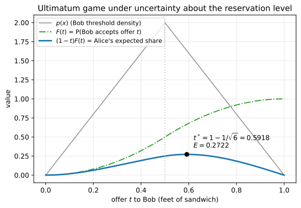
Alice’s problem. The grey triangle is the density \(p(x)\) of Bob’s unknown reservation level; the dash-dotted curve is the acceptance probability \(F(t)\); the heavy curve is her expected share \((1-t)F(t)\), maximized at \(t^*=1-1/\sqrt6\approx0.5918\) with value \(\sqrt6/9\approx0.2722\).
Two features are worth naming. Alice keeps the minority share, \(40.8\%\), where the complete-information subgame-perfect equilibrium would hand her nearly the whole sandwich: uncertainty about \(x\) alone, with no altruism or reciprocation in a one-shot game, drags the proposer’s demand below half. And she accepts a \(1/3\) chance of total breakdown rather than buying certainty (\(t = 0.75\) raises acceptance to \(87.5\%\) but drops her expected share to 0.219), so the expected total consumed is \(2/3\) of a foot and the ex-ante outcome \([0.272\;\;0.394]\) is not Pareto optimal.
Backlinks (4)
1. Reading List /words/reading-list/
As the years approach, I use this page to list out the books I intend to read.
Contrariwise, as the years goes by, I use this list to document the books I finished that year.
2020
- Make it Stick - Brown, Roediger, McDaniel
- How to Take Smart Notes - Sönke Ahrens
2021
- Meditations - Marcus Aurelius
- How to Read a Book - Mortimer J. Adler
- Moonwalking with Einstein - Joshua Foer
- One Up on Wall Street - Peter Lynch
2022
- Deep Work - Cal Newport
2025
- Kafka on the Shore - Murakami
- Think and Grow Rich - Napolean Hill
- Algorithms - Dasgupta
- Crime and Punishment - Dostoevsky
- Pro Git
- Understanding Analysis - Abbott
- Lord of the Flies - William Golding
- The Art of Statistics - David Spiegelhalter
2026
- A Mathematician’s Apology
- Zen and The Art of Motorcycle Maintainance
- Linux Pocket Guide - Daniel J. Barrett
- System Design Interview - Alex Xu
- Full-Stack Web Development with TypeScript 5 - Mykyta Chernenko
- Hamlet - Shakespeare
- The Count of Monte Cristo - Alexander Dumas (finish)
- Mathematics for Machine Learning Deisenroth, Faisal and Ong
- Dive into Design Patterns - Alexander Shvets
2027
- Designing Data-Intensive Applications - Kleppmann
- Efficient Linux at the Command Line - Daniel Barrett
- The Almanack of Naval Ravikant
- The Three Theban Plays - Sophocles
- Aeneid - Virgil
- Effective Python
- Learning Go
- All of Statistics - Larry Wasserman
2028
- Probability Theory: The Logic of Science - Jaynes
- Networked Life - Mung Chiang
- 48 Laws of Power
- Steve Jobs - Walter Isaacson
- Dickens
- Goethe
2029
- Probabilistic Machine Learning - Murphy
- Pushkin
- The Intelligent Investor - Benjamin Graham
2. Wiki /wiki/
Knowledge is a paradox. The more one understand, the more one realises the vastness of his ignorance.
3. Advanced Algorithms /wiki/ccs/dsa/advanced/
The content here-in has been influenced by Mung Chiang’s Networked Life and Introduction to Algorithms by CLRS.
4. Books /words/library/books/
Here are the books that I have taken the time to create metadata and/or notes for.
Comments