Solutions to Rosenthal’s A First Look at Rigorous Probability Theory
Solutions to every exercise in Jeffrey S. Rosenthal’s A First Look at Rigorous Probability Theory (2nd edition, World Scientific, 2006) — 203 exercises across chapters 1–14, from probability triples and the extension theorem through martingales. The book is filed at A First Look at Rigorous Probability Theory.
The Need for Measure Theory
Exercises 1.3.1–1.3.5
Suppose that \(\Omega = \{1,2\}\), with \(\mathbf{P}(\emptyset) = 0\) and \(\mathbf{P}\{1,2\} = 1\). Suppose \(\mathbf{P}\{1\} = \tfrac{1}{4}\). Prove that \(\mathbf{P}\) is countably additive if and only if \(\mathbf{P}\{2\} = \tfrac{3}{4}\).
(\(\Rightarrow\)) Apply countable additivity (1.2.3) to the disjoint sequence \(A_1 = \{1\}\), \(A_2 = \{2\}\), \(A_i = \emptyset\) for \(i \ge 3\):
\begin{equation*} 1 \;=\; \mathbf{P}\{1,2\} \;=\; \mathbf{P}\{1\} + \mathbf{P}\{2\} + \sum_{i \ge 3} \mathbf{P}(\emptyset) \;=\; \tfrac{1}{4} + \mathbf{P}\{2\}, \end{equation*}
so \(\mathbf{P}\{2\} = \tfrac{3}{4}\).
(\(\Leftarrow\)) Let \(A_1, A_2, \ldots \subseteq \Omega\) be disjoint. Empty terms contribute \(\mathbf{P}(\emptyset) = 0\) to both sides, and at most two of the \(A_i\) are non-empty.
(i) None non-empty: both sides are \(0\).
(ii) One non-empty, equal to \(A\): both sides equal \(\mathbf{P}(A)\).
(iii) Two non-empty: disjoint non-empty subsets of \(\{1,2\}\) must be \(\{1\}\) and \(\{2\}\), and
\begin{equation*} \mathbf{P}\bigl(\{1\} \cup \{2\}\bigr) \;=\; 1 \;=\; \tfrac{1}{4} + \tfrac{3}{4} \;=\; \mathbf{P}\{1\} + \mathbf{P}\{2\}. \end{equation*}
Suppose \(\Omega = \{1,2,3\}\) and \(\mathcal{F}\) is the collection of all subsets of \(\Omega\). Find (with proof) necessary and sufficient conditions on the real numbers \(x\), \(y\), and \(z\), such that there exists a countably additive probability measure \(\mathbf{P}\) on \(\mathcal{F}\), with \(x = \mathbf{P}\{1,2\}\), \(y = \mathbf{P}\{2,3\}\), and \(z = \mathbf{P}\{1,3\}\).
Such a \(\mathbf{P}\) exists if and only if
\begin{equation*} x + y + z = 2 \quad\text{and}\quad x \le 1,\; y \le 1,\; z \le 1 . \end{equation*}
(On a finite \(\Omega\) at most three of any disjoint \(A_1, A_2, \ldots\) are nonempty, so countable additivity (1.2.3) reduces to finite additivity.)
Necessity: additivity gives
\begin{equation*} \mathbf{P}\{1\} = 1 - y, \qquad \mathbf{P}\{2\} = 1 - z, \qquad \mathbf{P}\{3\} = 1 - x, \end{equation*}
so nonnegativity forces \(x, y, z \le 1\), and summing,
\begin{equation*} 1 = \mathbf{P}\{1\} + \mathbf{P}\{2\} + \mathbf{P}\{3\} = 3 - (x+y+z), \end{equation*}
i.e. \(x + y + z = 2\).
Sufficiency: given the conditions, put \(p_1 = 1-y\), \(p_2 = 1-z\), \(p_3 = 1-x\) and \(\mathbf{P}(A) = \sum_{i \in A} p_i\). The \(p_i\) are nonnegative and sum to \(3 - (x+y+z) = 1\), so \(\mathbf{P}\) is a countably additive probability measure, and using \(x+y+z = 2\),
\begin{equation*} \mathbf{P}\{1,2\} = 2 - (y+z) = x, \qquad \mathbf{P}\{2,3\} = y, \qquad \mathbf{P}\{1,3\} = z . \end{equation*}
Suppose that \(\Omega = \mathbf{N}\) is the set of positive integers, and \(\mathbf{P}\) is defined for all \(A \subseteq \Omega\) by \(\mathbf{P}(A) = 0\) if \(A\) is finite, and \(\mathbf{P}(A) = 1\) if \(A\) is infinite. Is \(\mathbf{P}\) finitely additive?
No. Take \(A\) to be the even positive integers and \(B\) the odd ones. They are disjoint, both are infinite, and \(A \cup B = \mathbf{N}\) is infinite, so
\begin{equation*} \mathbf{P}(A \cup B) \;=\; 1 \;\neq\; 2 \;=\; 1 + 1 \;=\; \mathbf{P}(A) + \mathbf{P}(B), \end{equation*}
contradicting (1.2.2).
Suppose that \(\Omega = \mathbf{N}\) (the set of positive integers), and \(\mathbf{P}\) is defined for all \(A \subseteq \Omega\) by \(\mathbf{P}(A) = |A|\) if \(A\) is finite (where \(|A|\) is the number of elements in the subset \(A\)), and \(\mathbf{P}(A) = \infty\) if \(A\) is infinite. This \(\mathbf{P}\) is of course not a probability measure (in fact it is counting measure), however we can still ask the following. (By convention, \(\infty + \infty = \infty\).)
- (a)
- Is \(\mathbf{P}\) finitely additive?
- (b)
- Is \(\mathbf{P}\) countably additive?
Yes to both. Arithmetic is in \([0,\infty]\), a nonnegative series being the supremum of its partial sums; note \(\mathbf{P}\) is monotone: \(A \subseteq B\) implies \(\mathbf{P}(A) \le \mathbf{P}(B)\).
(a) Let \(A \cap B = \emptyset\).
- (i) \(A, B\) finite: \(|A \cup B| = |A| + |B|\), so \(\mathbf{P}(A \cup B) = \mathbf{P}(A) + \mathbf{P}(B)\).
- (ii) one infinite, say \(A\): then \(A \cup B \supseteq A\) is infinite, and both sides equal \(\infty\).
By induction, \(\mathbf{P}(A_1 \cup \cdots \cup A_N) = \sum_{n=1}^{N} \mathbf{P}(A_n)\) for disjoint \(A_1, \ldots, A_N\).
(b) Let \(A_1, A_2, \ldots\) be disjoint with union \(A\). For every \(N\), part (a) and monotonicity give
\begin{equation*} \sum_{n=1}^{N} \mathbf{P}(A_n) = \mathbf{P}\!\left( \bigcup_{n=1}^{N} A_n \right) \le \mathbf{P}(A), \end{equation*}
so \(\sum_{n=1}^{\infty} \mathbf{P}(A_n) \le \mathbf{P}(A)\). Conversely:
- (i) \(A\) finite: only finitely many \(A_n\) are nonempty, so \(A = A_1 \cup \cdots \cup A_N\) for some \(N\) and equality holds by (a).
- (ii) \(A\) infinite: for each \(m\) pick \(m\) distinct points of \(A\); they lie in \(A_1 \cup \cdots \cup A_N\) for some finite \(N\), so by monotonicity and (a),
\begin{equation*} m \le \sum_{n=1}^{N} \mathbf{P}(A_n) \le \sum_{n=1}^{\infty} \mathbf{P}(A_n). \end{equation*}
Hence the series diverges and both sides equal \(\infty\).
(a) In what step of the proof of Proposition 1.2.6 was (1.2.1) used?
(b) Give an example of a countably additive set function \(\mathbf{P}\), defined on all subsets of \([0,1]\), which satisfies (1.2.3) and (1.2.5), but not (1.2.1).
(Here (1.2.1) is the interval formula \(\mathbf{P}([a,b]) = b - a\) for \(0 \le a \le b \le 1\), with the same value for \((a,b)\), \([a,b)\) and \((a,b]\); (1.2.3) is countable additivity; and (1.2.5) is shift-invariance \(\mathbf{P}(A \oplus r) = \mathbf{P}(A)\) for \(0 \le r \le 1\), where \(A \oplus r\) is the wrap-around \(r\)-shift defined in (1.2.4).)
(a) Only in the final display. Everything up to
\begin{equation*} \mathbf{P}\bigl((0,1]\bigr) \;=\; \sum_{\substack{r \in [0,1) \\ r \text{ rational}}} \mathbf{P}(H \oplus r) \;=\; \sum_{\substack{r \in [0,1) \\ r \text{ rational}}} \mathbf{P}(H) \end{equation*}
uses only the Axiom of Choice (to build \(H\)), countable additivity (1.2.3) for the disjoint shifts \(H \oplus r\) with union \((0,1]\), and shift-invariance (1.2.5). Equation (1.2.1) with \(a = 0\), \(b = 1\) enters only to evaluate the left side, \(\mathbf{P}((0,1]) = 1 - 0 = 1\), giving
\begin{equation*} 1 \;=\; \sum_{\substack{r \in [0,1) \\ r \text{ rational}}} \mathbf{P}(H), \end{equation*}
which is the contradiction: a countably infinite sum of copies of one constant is \(0\), \(+\infty\), or \(-\infty\), never \(1\).
(b) Take \(\mathbf{P}(A) = 0\) for every \(A \subseteq [0,1]\). Both sides of (1.2.3) are then \(0\) for any disjoint \(A_1, A_2, \ldots\), and \(\mathbf{P}(A \oplus r) = 0 = \mathbf{P}(A)\) gives (1.2.5); but \(\mathbf{P}([0,1]) = 0 \neq 1 - 0\), so (1.2.1) fails.
Method (2): \(\mathbf{P}(\emptyset) = 0\) and \(\mathbf{P}(A) = \infty\) for \(A \neq \emptyset\). For disjoint \(A_i\) both sides of (1.2.3) are \(0\) if every \(A_i = \emptyset\) and \(\infty\) otherwise; \(A \oplus r = \emptyset\) exactly when \(A = \emptyset\), giving (1.2.5); and \(\mathbf{P}([0,1]) = \infty \neq 1\).
Probability Triples
Exercises 2.7.1–2.7.7
Let \(\Omega = \{1,2,3,4\}\). Determine whether or not each of the following is a \(\sigma\)-algebra.
- (a)
- \(\mathcal{F}_1 = \bigl\{\emptyset,\ \{1,2\},\ \{3,4\},\ \{1,2,3,4\}\bigr\}\).
- (b)
- \(\mathcal{F}_2 = \bigl\{\emptyset,\ \{3\},\ \{4\},\ \{1,2\},\ \{3,4\},\ \{1,2,3\},\ \{1,2,4\},\ \{1,2,3,4\}\bigr\}\).
- (c)
- \(\mathcal{F}_3 = \bigl\{\emptyset,\ \{1,2\},\ \{1,3\},\ \{1,4\},\ \{2,3\},\ \{2,4\},\ \{3,4\},\ \{1,2,3,4\}\bigr\}\).
(a) Yes, (b) yes, (c) no.
On a finite \(\Omega\) every countable operation is a finite one, so the collection of all unions of blocks of a partition of \(\Omega\) is a \(\sigma\)-algebra.
(a) \(\mathcal{F}_1\) is exactly the four unions of blocks of the partition \(\{1,2\},\{3,4\}\). (Check!)
(b) \(\mathcal{F}_2\) is exactly the \(2^3 = 8\) unions of blocks of the partition \(\{1,2\},\{3\},\{4\}\):
\begin{equation*} \emptyset,\ \{1,2\},\ \{3\},\ \{4\},\ \{1,2,3\},\ \{1,2,4\},\ \{3,4\},\ \Omega . \end{equation*}
(c) \(\{1,2\},\{1,3\} \in \mathcal{F}_3\) but \(\{1,2\} \cup \{1,3\} = \{1,2,3\} \notin \mathcal{F}_3\), so \(\mathcal{F}_3\) is not closed under finite unions.
Let \(\Omega = \{1,2,3,4\}\), and let \(\mathcal{J} = \bigl\{\{1\},\{2\}\bigr\}\). Describe explicitly the \(\sigma\)-algebra \(\sigma(\mathcal{J})\) generated by \(\mathcal{J}\).
\begin{equation*} \sigma(\mathcal{J}) \;=\; \bigl\{\, \emptyset,\ \{1\},\ \{2\},\ \{3,4\},\ \{1,2\},\ \{1,3,4\},\ \{2,3,4\},\ \Omega \,\bigr\}. \end{equation*}
These are exactly the \(2^3\) unions of the atoms \(\{1\}, \{2\}, \{3,4\}\), which partition \(\Omega\), so the collection is a \(\sigma\)-algebra containing \(\mathcal{J}\); conversely any \(\sigma\)-algebra containing \(\{1\}\) and \(\{2\}\) contains \(\{1,2\}\), its complement \(\{3,4\}\), and hence all eight unions.
Suppose \(\mathcal{F}\) is a collection of subsets of \(\Omega\), such that \(\Omega \in \mathcal{F}\).
- (a)
- Suppose that whenever \(A, B \in \mathcal{F}\), then also \(A \setminus B \equiv A \cap B^C \in \mathcal{F}\). Prove that \(\mathcal{F}\) is an algebra.
- (b)
- Suppose \(\mathcal{F}\) is a semialgebra. Prove that \(\mathcal{F}\) is an algebra.
- (c)
- Suppose that \(\mathcal{F}\) is closed under complement, and also closed under finite disjoint unions (i.e. whenever \(A, B \in \mathcal{F}\) are disjoint, then \(A \cup B \in \mathcal{F}\)). Give a counter-example to show that \(\mathcal{F}\) might not be an algebra.
(a) Everything comes out of \(\Omega \in \mathcal{F}\) and the single closure rule:
\begin{equation*} \begin{aligned} \emptyset &= \Omega \setminus \Omega \in \mathcal{F}, \\ A^C &= \Omega \setminus A \in \mathcal{F}, \\ A \cap B &= A \setminus B^C \in \mathcal{F} \quad (\text{legal since } B^C \in \mathcal{F}), \\ A \cup B &= (A^C \cap B^C)^C \in \mathcal{F}. \end{aligned} \end{equation*}
So \(\mathcal{F}\) contains \(\Omega\) and \(\emptyset\) and is closed under complement and finite unions and intersections, i.e. it is an algebra.
(b) As printed this is false – the semialgebra \(\mathcal{J}\) of all intervals in \([0,1]\) (Exercise 2.2.3) has \((0,\tfrac14]^C = \{0\} \cup (\tfrac14, 1] \notin \mathcal{J}\) – so read the intended hypothesis: \(\mathcal{F}\) is a semialgebra that is moreover closed under finite disjoint unions. Then for \(A \in \mathcal{F}\) the semialgebra property writes
\begin{equation*} A^C = J_1 \cup \cdots \cup J_k , \qquad J_1,\dots,J_k \in \mathcal{F} \ \text{disjoint}, \end{equation*}
so \(A^C \in \mathcal{F}\) by that added closure; \(\mathcal{F}\) is closed under finite intersections by the definition of semialgebra; and then \(A \cup B = (A^C \cap B^C)^C \in \mathcal{F}\). Since \(\emptyset, \Omega \in \mathcal{F}\), this is an algebra.
(c) Take \(\Omega = \{1,2,3,4\}\) and
\begin{equation*} \mathcal{F} = \bigl\{\emptyset,\ \{1,2\},\ \{1,3\},\ \{1,4\},\ \{2,3\},\ \{2,4\},\ \{3,4\},\ \Omega\bigr\}, \end{equation*}
the family of Exercise 2.7.1(c). Complementation permutes the six two-element sets and swaps \(\emptyset\) with \(\Omega\). Any two disjoint non-empty members are two-element sets using all \(2 + 2 = 4\) points, hence complementary, with union \(\Omega \in \mathcal{F}\); a third non-empty member cannot be adjoined, and \(\emptyset\) contributes nothing. So \(\mathcal{F}\) is closed under finite disjoint unions. But
\begin{equation*} \{1,2\} \cup \{1,3\} = \{1,2,3\} \notin \mathcal{F}, \end{equation*}
so \(\mathcal{F}\) is not an algebra.
Let \(\mathcal{F}_1, \mathcal{F}_2, \ldots\) be a sequence of collections of subsets of \(\Omega\), such that \(\mathcal{F}_n \subseteq \mathcal{F}_{n+1}\) for each \(n\).
- (a)
- Suppose that each \(\mathcal{F}_i\) is an algebra. Prove that \(\bigcup_{i=1}^{\infty} \mathcal{F}_i\) is also an algebra.
- (b)
- Suppose that each \(\mathcal{F}_i\) is a \(\sigma\)-algebra. Show (by counter-example) that \(\bigcup_{i=1}^{\infty} \mathcal{F}_i\) might not be a \(\sigma\)-algebra.
Write \(\mathcal{F} = \bigcup_{i=1}^{\infty} \mathcal{F}_i\); since the sequence is increasing, any finitely many members \(A_1, \ldots, A_k\) of \(\mathcal{F}\) lie in a common \(\mathcal{F}_N\) (take \(N\) the largest of their indices).
(a) \(\emptyset, \Omega \in \mathcal{F}_1 \subseteq \mathcal{F}\). If \(A \in \mathcal{F}_n\) then \(A^{C} \in \mathcal{F}_n \subseteq \mathcal{F}\). If \(A_1, \ldots, A_k \in \mathcal{F}_N\) then \(\bigcup_{j} A_j \in \mathcal{F}_N \subseteq \mathcal{F}\), and intersections follow by De Morgan. Hence \(\mathcal{F}\) is an algebra (Exercise 2.2.5).
(b) Take \(\Omega = \mathbf{N}\) and let \(\mathcal{F}_n\) consist of all unions of blocks of the partition
\begin{equation*} \mathcal{P}_n = \bigl\{ \{1\}, \ldots, \{n\},\ T_n \bigr\}, \qquad T_n = \{n+1, n+2, \ldots\}; \end{equation*}
explicitly, \(\mathcal{F}_n = \{ S \text{ or } S \cup T_n : S \subseteq \{1,\ldots,n\} \}\). Unions of blocks of a partition always form a \(\sigma\)-algebra (as in 2.7.2), and \(\mathcal{F}_n \subseteq \mathcal{F}_{n+1}\) since \(T_n = \{n+1\} \cup T_{n+1}\). Every singleton \(\{k\}\) lies in \(\mathcal{F}_k \subseteq \mathcal{F}\), but the even numbers \(E = \bigcup_{k} \{2k\}\) lie in no \(\mathcal{F}_n\): a member of \(\mathcal{F}_n\) either is contained in \(\{1,\ldots,n\}\) (impossible, as \(2n+2 \in E\)) or contains \(T_n\) (impossible, as one of \(n+1, n+2 \in T_n\) is odd). So \(\mathcal{F}\) is not closed under countable unions.
Suppose that \(\Omega = \mathbf{N}\) is the set of positive integers, and \(\mathcal{F}\) is the set of all subsets \(A\) such that either \(A\) or \(A^C\) is finite, and \(\mathbf{P}\) is defined by \(\mathbf{P}(A) = 0\) if \(A\) is finite, and \(\mathbf{P}(A) = 1\) if \(A^C\) is finite.
- (a)
- Is \(\mathcal{F}\) an algebra?
- (b)
- Is \(\mathcal{F}\) a \(\sigma\)-algebra?
- (c)
- Is \(\mathbf{P}\) finitely additive?
- (d)
- Is \(\mathbf{P}\) countably additive on \(\mathcal{F}\), meaning that if \(A_1, A_2, \ldots \in \mathcal{F}\) are disjoint, and if it happens that \(\bigcup_n A_n \in \mathcal{F}\), then \(\mathbf{P}\bigl(\bigcup_n A_n\bigr) = \sum_n \mathbf{P}(A_n)\)?
(a) Yes, (b) no, (c) yes, (d) no. (\(\mathbf{P}\) is unambiguous because \(\mathbf{N}\) is infinite, so \(A\) and \(A^C\) are never both finite.)
(a) \(\Omega \in \mathcal{F}\) since \(\Omega^C = \emptyset\) is finite, and \(\emptyset \in \mathcal{F}\); the defining condition is symmetric in \(A, A^C\), so \(\mathcal{F}\) is closed under complement. For \(A, B \in \mathcal{F}\): if both are finite then \(A \cup B\) is finite, and otherwise (say \(A^C\) finite) \((A\cup B)^C = A^C \cap B^C \subseteq A^C\) is finite. Either way \(A \cup B \in \mathcal{F}\), and \(A \cap B = (A^C \cup B^C)^C \in \mathcal{F}\).
(b) Take \(A_n = \{2n\}\), each finite hence in \(\mathcal{F}\). Then \(\bigcup_n A_n\) is the set of even integers, which is infinite and has infinite complement, so it is not in \(\mathcal{F}\).
(c) Let \(A, B \in \mathcal{F}\) be disjoint. They cannot both be cofinite: \(B \subseteq A^C\), so if \(A^C\) is finite then \(B\) is finite. Hence:
- (i)
- both finite: \(A \cup B\) is finite and \(0 = 0 + 0\);
- (ii)
- \(A^C\) finite (so \(B\) finite): \((A \cup B)^C \subseteq A^C\) is finite, and \(1 = 1 + 0\).
Induction on the number of sets extends this to any finite disjoint family.
(d) Take \(A_n = \{n\}\). These are disjoint elements of \(\mathcal{F}\) and \(\bigcup_n A_n = \mathbf{N} = \Omega \in \mathcal{F}\), yet
\begin{equation*} \mathbf{P}\Bigl(\bigcup_n A_n\Bigr) = \mathbf{P}(\Omega) = 1 \neq 0 = \sum_n \mathbf{P}(A_n). \end{equation*}
Suppose that \(\Omega = [0,1]\) is the unit interval, and \(\mathcal{F}\) is the set of all subsets \(A\) such that either \(A\) or \(A^{C}\) is finite, and \(\mathbf{P}\) is defined by \(\mathbf{P}(A) = 0\) if \(A\) is finite, and \(\mathbf{P}(A) = 1\) if \(A^{C}\) is finite.
- (a)
- Is \(\mathcal{F}\) an algebra?
- (b)
- Is \(\mathcal{F}\) a \(\sigma\)-algebra?
- (c)
- Is \(\mathbf{P}\) finitely additive?
- (d)
- Is \(\mathbf{P}\) countably additive on \(\mathcal{F}\) (as in the previous exercise), meaning that if \(A_1, A_2, \ldots \in \mathcal{F}\) are disjoint, and if it happens that \(\bigcup_n A_n \in \mathcal{F}\), then \(\mathbf{P}\bigl(\bigcup_n A_n\bigr) = \sum_n \mathbf{P}(A_n)\)?
(a) Yes. \(\emptyset, \Omega \in \mathcal{F}\); the defining condition is symmetric under \(A \leftrightarrow A^{C}\); and for \(A, B \in \mathcal{F}\): if both are finite so is \(A \cup B\), while if (say) \(A^{C}\) is finite then \((A \cup B)^{C} \subseteq A^{C}\) is finite. Intersections follow by De Morgan, so \(\mathcal{F}\) is an algebra (Exercise 2.2.5).
(b) No. Each \(\{1/n\} \in \mathcal{F}\), but \(A = \{1/n : n \in \mathbf{N}\}\) is infinite with uncountable (hence infinite) complement, so \(A \notin \mathcal{F}\).
(c) Yes. Let \(A, B \in \mathcal{F}\) be disjoint (they cannot both be co-finite, else \(\Omega\) would be finite).
- (i) \(A, B\) finite: both sides are \(0\).
- (ii) say \(A^{C}\) finite: then \(B \subseteq A^{C}\) is finite and \((A \cup B)^{C} \subseteq A^{C}\) is finite, so \(\mathbf{P}(A \cup B) = 1 = 1 + 0 = \mathbf{P}(A) + \mathbf{P}(B)\).
(d) Yes. Let \(A_1, A_2, \ldots \in \mathcal{F}\) be disjoint with \(A = \bigcup_n A_n \in \mathcal{F}\); at most one \(A_n\) is co-finite, as in (c).
- (i) every \(A_n\) finite: \(A\) is countable, and a countable set cannot be co-finite in the uncountable \([0,1]\), so \(A\) is finite and \(\mathbf{P}(A) = 0 = \sum_n \mathbf{P}(A_n)\).
- (ii) \(A_{n_0}^{C}\) finite: each \(A_n\) with \(n \ne n_0\) lies in \(A_{n_0}^{C}\), hence is finite with \(\mathbf{P}(A_n) = 0\), and \(A^{C} \subseteq A_{n_0}^{C}\) is finite, so both sides equal \(1\).
Suppose that \(\Omega = [0,1]\) is the unit interval, and \(\mathcal{F}\) is the set of all subsets \(A\) such that either \(A\) or \(A^C\) is countable (i.e., finite or countably infinite), and \(\mathbf{P}\) is defined by \(\mathbf{P}(A) = 0\) if \(A\) is countable, and \(\mathbf{P}(A) = 1\) if \(A^C\) is countable.
- (a)
- Is \(\mathcal{F}\) an algebra?
- (b)
- Is \(\mathcal{F}\) a \(\sigma\)-algebra?
- (c)
- Is \(\mathbf{P}\) finitely additive?
- (d)
- Is \(\mathbf{P}\) countably additive on \(\mathcal{F}\)?
Yes to all four. Everything rests on two facts: \([0,1]\) is uncountable (so no \(A\) has both \(A\) and \(A^C\) countable, and \(\mathbf{P}\) is unambiguous), and a countable union of countable sets is countable.
(a), (b). \(\emptyset, \Omega \in \mathcal{F}\), and the defining condition is symmetric in \(A, A^C\), so \(\mathcal{F}\) is closed under complement. Let \(A_1, A_2, \ldots \in \mathcal{F}\) and \(A = \bigcup_n A_n\):
- (i)
- every \(A_n\) countable: then \(A\) is a countable union of countable sets, hence countable, so \(A \in \mathcal{F}\);
- (ii)
- some \(A_{n_0}^C\) countable: then \(A^C \subseteq A_{n_0}^C\) is countable, so \(A \in \mathcal{F}\).
Closure under countable intersections follows by De Morgan, so \(\mathcal{F}\) is a \(\sigma\)-algebra, in particular an algebra.
(c), (d). Finite additivity is the case \(A_n = \emptyset\) for all large \(n\), so only the countable statement needs proof. Let \(A_1, A_2, \ldots \in \mathcal{F}\) be disjoint, \(A = \bigcup_n A_n\). At most one \(A_n\) can be co-countable, since for \(m \neq n\) disjointness gives \(A_m \subseteq A_n^C\). Two cases, matching those above:
- (i)
- every \(A_n\) countable. Then \(A\) is countable and \(\mathbf{P}(A) = 0 = \sum_n \mathbf{P}(A_n)\).
- (ii)
- \(A_{n_0}^C\) countable for exactly one \(n_0\). Then \(A_n \subseteq A_{n_0}^C\) is countable for \(n \neq n_0\), while \(A^C \subseteq A_{n_0}^C\) is countable, so
\begin{equation*} \mathbf{P}(A) = 1 = \mathbf{P}(A_{n_0}) = \sum_n \mathbf{P}(A_n). \end{equation*}
Exercises 2.7.8–2.7.14
For the example of Exercise 2.7.7, is \(\mathbf{P}\) uncountably additive (cf. page 2)?
Here Exercise 2.7.7 is the following example: \(\Omega = [0,1]\) is the unit interval, \(\mathcal{F}\) is the set of all subsets \(A\) such that either \(A\) or \(A^{C}\) is countable (i.e. finite or countably infinite), and \(\mathbf{P}\) is defined by \(\mathbf{P}(A) = 0\) if \(A\) is countable, and \(\mathbf{P}(A) = 1\) if \(A^{C}\) is countable.
Uncountable additivity means the following. Recall the convention recorded in Subsection 1.2 (cf. Subsection A.2): for a non-negative uncountable collection \(\{r_\alpha\}_{\alpha \in I}\), the sum \(\sum_{\alpha \in I} r_\alpha\) is defined to be the supremum of \(\sum_{\alpha \in J} r_\alpha\) over finite subsets \(J \subseteq I\). The question is whether, for every collection \(\{A_\alpha\}_{\alpha \in I} \subseteq \mathcal{F}\) of disjoint sets indexed by an arbitrary (possibly uncountable) set \(I\) with \(\bigcup_{\alpha \in I} A_\alpha \in \mathcal{F}\), one has \(\mathbf{P}\bigl(\bigcup_{\alpha \in I} A_\alpha\bigr) = \sum_{\alpha \in I} \mathbf{P}(A_\alpha)\).
No. The disjoint singletons \(\{x\}\), \(x \in [0,1]\), all lie in \(\mathcal{F}\) with \(\mathbf{P}\{x\} = 0\), and their union is \(\Omega \in \mathcal{F}\); but every finite partial sum of the \(\mathbf{P}\{x\}\) is \(0\), so
\begin{equation*} 1 \;=\; \mathbf{P}\Bigl( \bigcup_{x \in [0,1]} \{x\} \Bigr) \;\ne\; \sum_{x \in [0,1]} \mathbf{P}\{x\} \;=\; 0 , \end{equation*}
the same decomposition used on page 2.
Let \(\mathcal{F}\) be a \(\sigma\)-algebra, and write \(|\mathcal{F}|\) for the total number of subsets in \(\mathcal{F}\). Prove that if \(|\mathcal{F}| < \infty\) (i.e., if \(\mathcal{F}\) consists of just a finite number of subsets), then \(|\mathcal{F}| = 2^m\) for some \(m \in \mathbf{N}\). [Hint: Consider those non-empty subsets in \(\mathcal{F}\) which do not contain any other non-empty subset in \(\mathcal{F}\). How can all subsets in \(\mathcal{F}\) be “built up” from these particular subsets?]
The atoms are the sets
\begin{equation*} A_\omega \ = \bigcap_{A \in \mathcal{F},\ \omega \in A} A , \qquad \omega \in \Omega , \end{equation*}
each of which lies in \(\mathcal{F}\) because the intersection is over a finite subfamily of \(\mathcal{F}\), and is non-empty, containing \(\omega\). By construction \(A_\omega\) is contained in every member of \(\mathcal{F}\) that contains \(\omega\); these are the hint’s minimal non-empty sets.
Distinct atoms are disjoint. Suppose \(\omega^{\prime} \in A_\omega\); we claim \(A_{\omega^{\prime}} = A_\omega\). Certainly \(A_{\omega^{\prime}} \subseteq A_\omega\), since \(A_\omega\) is a member of \(\mathcal{F}\) containing \(\omega^{\prime}\). If \(\omega \in A_{\omega^{\prime}}\) then symmetrically \(A_\omega \subseteq A_{\omega^{\prime}}\) and we are done; if instead \(\omega \notin A_{\omega^{\prime}}\), then \(B = A_\omega \cap A_{\omega^{\prime}}^C \in \mathcal{F}\) contains \(\omega\), so \(A_\omega \subseteq B \subseteq A_{\omega^{\prime}}^C\), contradicting \(\omega^{\prime} \in A_\omega \cap A_{\omega^{\prime}}\). Hence if \(\omega^{\prime\prime} \in A_\omega \cap A_{\omega^{\prime}}\) then \(A_\omega = A_{\omega^{\prime\prime}} = A_{\omega^{\prime}}\), so two atoms are either equal or disjoint.
Since \(\omega \in A_\omega\), the distinct atoms partition \(\Omega\), and being members of the finite collection \(\mathcal{F}\) there are finitely many of them, say \(A_1, \ldots, A_m\).
Every member of \(\mathcal{F}\) is a union of atoms, uniquely. For \(A \in \mathcal{F}\) and \(\omega \in A\) we have \(A_\omega \subseteq A\), whence
\begin{equation*} A \ = \bigcup_{\omega \in A} A_\omega \ = \bigcup_{i \,:\, A_i \subseteq A} A_i , \end{equation*}
a union of a subcollection \(S_A \subseteq \{A_1,\dots,A_m\}\). Conversely every union \(\bigcup_{i \in S} A_i\) over \(S \subseteq \{1,\dots,m\}\) lies in \(\mathcal{F}\), being a finite union of members of \(\mathcal{F}\). The map \(S \mapsto \bigcup_{i \in S} A_i\) is injective because the \(A_i\) are non-empty and pairwise disjoint: \(A_j \subseteq \bigcup_{i \in S} A_i\) forces \(j \in S\). So \(S \mapsto \bigcup_{i \in S} A_i\) is a bijection from the subsets of \(\{1,\dots,m\}\) onto \(\mathcal{F}\), and
\begin{equation*} |\mathcal{F}| \ = \ 2^m . \end{equation*}
Prove that the collection \(\mathcal{J}\) of (2.5.10) is a semialgebra.
Here (2.5.10), from the proof of Corollary 2.5.9, is the collection of subsets of \(\Omega = \mathbf{R}\) given by
\begin{equation*} \begin{aligned} \mathcal{J} \;=\;& \bigl\{ (-\infty, x] : x \in \mathbf{R} \bigr\} \\ &\cup\ \bigl\{ (y, \infty) : y \in \mathbf{R} \bigr\} \\ &\cup\ \bigl\{ (x,y] : x, y \in \mathbf{R} \bigr\} \\ &\cup\ \bigl\{ \emptyset, \mathbf{R} \bigr\}. \end{aligned} \end{equation*}
(The printed text has the misprint \((\infty, x]\) for \((-\infty, x]\).) Recall from Exercise 2.2.3 that a collection \(\mathcal{J}\) of subsets of \(\Omega\) is a semialgebra if it contains \(\emptyset\) and \(\Omega\), it is closed under finite intersection, and the complement of any element of \(\mathcal{J}\) is equal to a finite disjoint union of elements of \(\mathcal{J}\).
Every member of \(\mathcal{J}\) has the normal form
\begin{equation*} I(a,b] \;=\; \{\, t \in \mathbf{R} : a < t \le b \,\}, \qquad a \le b \text{ in } [-\infty, +\infty], \end{equation*}
and conversely every such set lies in \(\mathcal{J}\): \((-\infty,x] = I(-\infty,x]\), \((y,\infty) = I(y,+\infty]\), \((x,y] = I(x,y]\) (or \(\emptyset\) if \(x > y\)), \(\mathbf{R} = I(-\infty,+\infty]\), \(\emptyset = I(0,0]\). (Check!) The three semialgebra properties (Exercise 2.2.3) now follow.
- (i) \(\emptyset = I(0,0]\) and \(\mathbf{R} = I(-\infty,+\infty]\) lie in \(\mathcal{J}\).
- (ii) Intersections:
\begin{equation*} I(a,b] \cap I(c,d] \;=\; I\bigl( \max(a,c),\, \min(b,d) \bigr] \;\in\; \mathcal{J} \end{equation*}
(empty when \(\max(a,c) > \min(b,d)\)); pairwise closure gives finite closure by induction.
- (iii) Complements:
\begin{equation*} \bigl( I(a,b] \bigr)^{C} \;=\; I(-\infty, a] \;\cup\; I(b, +\infty], \end{equation*}
a disjoint union of two members of \(\mathcal{J}\).
Hence \(\mathcal{J}\) is a semialgebra.
Let \(\Omega = [0,1]\). Let \(\mathcal{J}^{\prime}\) be the set of all half-open intervals of the form \((a,b]\), for \(0 \le a < b \le 1\), together with the sets \(\emptyset\), \(\Omega\), and \(\{0\}\).
- (a)
- Prove that \(\mathcal{J}^{\prime}\) is a semialgebra.
- (b)
- Prove that \(\sigma(\mathcal{J}^{\prime}) = \mathcal{B}\), i.e. that the \(\sigma\)-algebra generated by this \(\mathcal{J}^{\prime}\) is equal to the \(\sigma\)-algebra generated by the \(\mathcal{J}\) of (2.4.1), namely \(\mathcal{J} = \{\text{all intervals contained in } [0,1]\}\).
- (c)
- Let \(\mathcal{B}_0^{\prime}\) be the collection of all finite disjoint unions of elements of \(\mathcal{J}^{\prime}\). Prove that \(\mathcal{B}_0^{\prime}\) is an algebra. Is \(\mathcal{B}_0^{\prime}\) the same as the algebra \(\mathcal{B}_0\) of (2.2.4), namely the collection of all finite unions of elements of \(\mathcal{J}\)?
[Remark: Some treatments of Lebesgue measure use \(\mathcal{J}^{\prime}\) instead of \(\mathcal{J}\).]
(a) The three requirements of the definition of semialgebra (Exercise 2.2.3) are immediate. \(\emptyset, \Omega \in \mathcal{J}^{\prime}\) by fiat. For intersections, \(\Omega\) and \(\emptyset\) are neutral and absorbing, \(\{0\} \cap (a,b] = \emptyset\) because \(a \ge 0\) puts \(0 \notin (a,b]\), and
\begin{equation*} (a,b] \cap (c,d] \ = \ \bigl(\max(a,c),\, \min(b,d)\bigr] , \end{equation*}
which is again of that form when \(\max(a,c) < \min(b,d)\) and is \(\emptyset\) otherwise. For complements, \(\emptyset^C = \Omega\), \(\Omega^C = \emptyset\), \(\{0\}^C = (0,1]\), and
\begin{equation*} (a,b]^C \ = \ \{0\} \cup (0,a] \cup (b,1] , \end{equation*}
a disjoint union of elements of \(\mathcal{J}^{\prime}\) (omit \((0,a]\) if \(a = 0\), and omit \((b,1]\) if \(b = 1\)).
(b) \(\mathcal{J}^{\prime} \subseteq \mathcal{J}\), since \(\emptyset\), the singleton \(\{0\}\), the interval \(\Omega = [0,1]\) and the half-open intervals \((a,b]\) are all intervals contained in \([0,1]\); hence \(\sigma(\mathcal{J}^{\prime}) \subseteq \sigma(\mathcal{J}) = \mathcal{B}\).
For the reverse, it suffices to put every interval \(I \subseteq [0,1]\) into \(\sigma(\mathcal{J}^{\prime})\). All singletons are there:
\begin{equation*} \{0\} \in \mathcal{J}^{\prime} , \qquad \{b\} \ = \ \bigcap_{n > 1/b} \bigl(b - \tfrac1n,\, b\bigr] \in \sigma(\mathcal{J}^{\prime}) \quad (0 < b \le 1). \end{equation*}
Then for \(0 \le a < b \le 1\),
\begin{equation*} \begin{aligned} (a,b] &\in \mathcal{J}^{\prime} , \\ [a,b] &= \{a\} \cup (a,b] \in \sigma(\mathcal{J}^{\prime}) , \\ (a,b) &= (a,b] \setminus \{b\} \in \sigma(\mathcal{J}^{\prime}) , \\ [a,b) &= \{a\} \cup (a,b) \in \sigma(\mathcal{J}^{\prime}) , \end{aligned} \end{equation*}
and the degenerate intervals \(\emptyset\) and \(\{a\}\) are already handled. Hence \(\mathcal{J} \subseteq \sigma(\mathcal{J}^{\prime})\), so \(\mathcal{B} = \sigma(\mathcal{J}) \subseteq \sigma(\mathcal{J}^{\prime})\), and the two \(\sigma\)-algebras coincide.
(c) \(\emptyset, \Omega \in \mathcal{J}^{\prime} \subseteq \mathcal{B}_0^{\prime}\). If \(A = \bigcup_{i=1}^n A_i\) and \(B = \bigcup_{j=1}^k B_j\) are disjoint unions of elements of \(\mathcal{J}^{\prime}\), then
\begin{equation*} A \cap B \ = \ \bigcup_{i=1}^{n} \bigcup_{j=1}^{k} (A_i \cap B_j) , \end{equation*}
and the sets \(A_i \cap B_j\) lie in \(\mathcal{J}^{\prime}\) (part (a)) and are pairwise disjoint; so \(\mathcal{B}_0^{\prime}\) is closed under finite intersections. For complements, by part (a) each \(A_i^C\) is a finite disjoint union of elements of \(\mathcal{J}^{\prime}\), i.e. \(A_i^C \in \mathcal{B}_0^{\prime}\), so
\begin{equation*} A^C \ = \ \bigcap_{i=1}^n A_i^C \ \in \ \mathcal{B}_0^{\prime} \end{equation*}
by the closure just proved. Finally \(A \cup B = (A^C \cap B^C)^C \in \mathcal{B}_0^{\prime}\). Hence \(\mathcal{B}_0^{\prime}\) is an algebra.
It is not the same as \(\mathcal{B}_0\): since \(\mathcal{J}^{\prime} \subseteq \mathcal{J}\) we have \(\mathcal{B}_0^{\prime} \subseteq \mathcal{B}_0\), but the containment is strict, because \(\{1/2\} \in \mathcal{J} \subseteq \mathcal{B}_0\) while \(\{1/2\} \notin \mathcal{B}_0^{\prime}\): an element of \(\mathcal{B}_0^{\prime}\) equal to \(\{1/2\}\) could use neither \(\Omega\) nor \(\{0\}\) as a piece, and every non-empty piece \((a,b]\) is uncountable.
Let \(K\) be the Cantor set as defined in Subsection 2.4. Let \(D_n = K \oplus \frac{1}{n}\) where \(K \oplus \frac{1}{n}\) is defined as in (1.2.4), namely
\begin{equation*} A \oplus r \;=\; \{\, a + r \;:\; a \in A,\ a + r \le 1 \,\} \cup \{\, a + r - 1 \;:\; a \in A,\ a + r > 1 \,\} \end{equation*}
for \(0 \le r \le 1\) (the \(r\)-shift of \(A \subseteq [0,1]\), with wrap-around). Let \(B = \bigcup_{n=1}^{\infty} D_n\).
- (a)
- Draw a rough sketch of \(D_3\).
- (b)
- What is \(\lambda(D_3)\)?
- (c)
- Draw a rough sketch of \(B\).
- (d)
- What is \(\lambda(B)\)?
(a), (c) The sketches are below: the top panel is \(D_3\), the bottom panel builds \(B\) up through \(D_1\), \(D_1 \cup D_2\), \(D_1 \cup D_2 \cup D_3\).
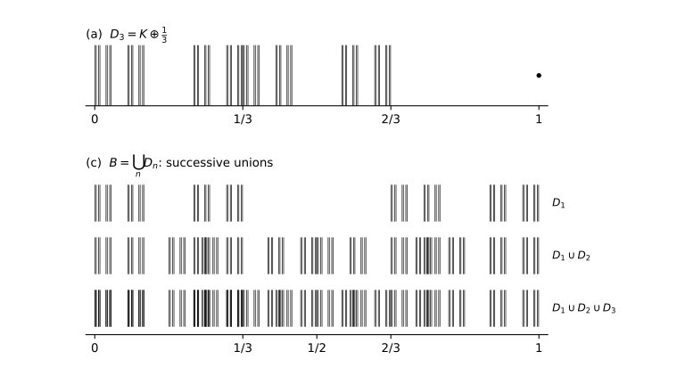
For (a): since \(K\) misses \((1/3, 2/3)\) and its two halves are \(K \cap [0,1/3] = \frac{1}{3}K\) and \(K \cap [2/3,1] = \frac{2}{3} + \frac{1}{3}K\), unwinding (1.2.4) with \(r = 1/3\) gives
\begin{equation*} D_3 \;=\; \Bigl( \tfrac{1}{3}K \setminus \{0\} \Bigr) \;\cup\; \Bigl( \tfrac{1}{3}K + \tfrac{1}{3} \Bigr) \;\cup\; \{1\} : \end{equation*}
two scale-\(1/3\) Cantor sets filling \([0, 2/3]\), plus the lone point \(1\). For (c): \(D_n\) is the bulk of \(K\) slid right by \(1/n\) with the right-hand sliver wrapped into \((0, 1/n]\); in particular \(D_1 = K \setminus \{0\}\) (since \(1 \in K\)). So \(B\) superimposes shifted copies of \(K\) for all \(n\), a dust that accumulates on \(K\) as \(1/n \to 0\) but (by (d)) contains no interval.
(b) \(\lambda(D_3) = 0\): \(D_3\) is a union of two translates of subsets of the null set \(K\) (Subsection 2.4), a translated-and-truncated interval cover shows translates of null sets are null, and null sets lie in \(\mathcal{M}\) with measure \(0\) (completeness, Exercise 2.3.16).
(d) \(\lambda(B) = 0\): as in (b) each \(\lambda(D_n) = 0\), so by countable subadditivity
\begin{equation*} \lambda(B) \;\le\; \sum_{n=1}^{\infty} \lambda(D_n) \;=\; 0 . \end{equation*}
Give an example of a sample space \(\Omega\), a semialgebra \(\mathcal{J}\), and a non-negative function \(\mathbf{P} : \mathcal{J} \to \mathbf{R}\) with \(\mathbf{P}(\emptyset) = 0\) and \(\mathbf{P}(\Omega) = 1\), such that (2.5.5) is not satisfied, i.e. such that the countable additivity property
\begin{equation*} \mathbf{P}\Bigl(\bigcup_n D_n\Bigr) \ = \ \sum_n \mathbf{P}(D_n) \end{equation*}
fails for some disjoint \(D_1, D_2, \ldots \in \mathcal{J}\) with \(\bigcup_n D_n \in \mathcal{J}\).
Take \(\Omega = \mathbf{N}\), let \(\mathcal{J}\) be the collection of all subsets of \(\mathbf{N}\), and set
\begin{equation*} \mathbf{P}(A) \ = \ \begin{cases} 0, & A \text{ finite}, \\ 1, & A \text{ infinite}. \end{cases} \end{equation*}
\(\mathcal{J}\) is a \(\sigma\)-algebra, hence a semialgebra: it contains \(\emptyset\) and \(\Omega\), it is closed under finite intersection, and \(A^C \in \mathcal{J}\) is a (one-term) finite disjoint union of elements of \(\mathcal{J}\). Also \(\mathbf{P} \ge 0\) with \(\mathbf{P}(\emptyset) = 0\) and \(\mathbf{P}(\Omega) = \mathbf{P}(\mathbf{N}) = 1\).
But \(D_n = \{n\}\) gives disjoint \(D_1, D_2, \ldots \in \mathcal{J}\) with \(\bigcup_n D_n = \mathbf{N} \in \mathcal{J}\), and
\begin{equation*} \mathbf{P}\Bigl(\bigcup_n D_n\Bigr) \ = \ 1 \ \neq \ 0 \ = \ \sum_n \mathbf{P}(D_n) , \end{equation*}
so (2.5.5) fails.
Let \(\Omega = \{1,2,3,4\}\), with \(\mathcal{F}\) the collection of all subsets of \(\Omega\). Let \(\mathbf{P}\) and \(\mathbf{Q}\) be two probability measures on \(\mathcal{F}\), such that
\begin{equation*} \mathbf{P}\{1\} = \mathbf{P}\{2\} = \mathbf{P}\{3\} = \mathbf{P}\{4\} = 1/4, \end{equation*}
and \(\mathbf{Q}\{2\} = \mathbf{Q}\{4\} = 1/2\), extended to \(\mathcal{F}\) by linearity. Finally, let
\begin{equation*} \mathcal{J} \;=\; \bigl\{ \emptyset,\ \Omega,\ \{1,2\},\ \{2,3\},\ \{3,4\},\ \{1,4\} \bigr\}. \end{equation*}
- (a)
- Prove that \(\mathbf{P}(A) = \mathbf{Q}(A)\) for all \(A \in \mathcal{J}\).
- (b)
- Prove that there is \(A \in \sigma(\mathcal{J})\) with \(\mathbf{P}(A) \ne \mathbf{Q}(A)\).
- (c)
- Why does this not contradict Proposition 2.5.8?
Note \(\mathbf{Q}\{1\} = \mathbf{Q}\{3\} = 0\), since \(\mathbf{Q}\{2\} + \mathbf{Q}\{4\} = 1\) already.
(a) Both measures give \(\emptyset\) probability \(0\) and \(\Omega\) probability \(1\), and every other member of \(\mathcal{J}\) is a pair containing exactly one even and one odd point, so for such \(A\)
\begin{equation*} \mathbf{P}(A) = \tfrac14 + \tfrac14 = \tfrac12 = \tfrac12 + 0 = \mathbf{Q}(A). \end{equation*}
(b) \(\{2\} = \{1,2\} \cap \{2,3\} \in \sigma(\mathcal{J})\), and
\begin{equation*} \mathbf{P}\{2\} = \tfrac14 \;\ne\; \tfrac12 = \mathbf{Q}\{2\}. \end{equation*}
(c) \(\mathcal{J}\) is not a semialgebra: \(\{1,2\} \cap \{2,3\} = \{2\} \notin \mathcal{J}\), so \(\mathcal{J}\) is not closed under finite intersection (Exercise 2.2.3) and Proposition 2.5.8 does not apply.
Exercises 2.7.15–2.7.21
Let \((\Omega,\mathcal{M},\lambda)\) be Lebesgue measure on the interval \([0,1]\). Let
\begin{equation*} \Omega^{\prime} \;=\; \bigl\{(x,y)\in\mathbf{R}^2 ;\ 0<x\le 1,\ 0<y\le 1\bigr\}. \end{equation*}
Let \(\mathcal{F}\) be the collection of all subsets of \(\Omega^{\prime}\) of the form
\begin{equation*} \bigl\{(x,y)\in\mathbf{R}^2 ;\ x\in A,\ 0<y\le 1\bigr\} \end{equation*}
for some \(A\in\mathcal{M}\). Finally, define a probability \(\mathbf{P}\) on \(\mathcal{F}\) by
\begin{equation*} \mathbf{P}\bigl(\{(x,y)\in\mathbf{R}^2 ;\ x\in A,\ 0<y\le 1\}\bigr) \;=\; \lambda(A). \end{equation*}
(a) Prove that \((\Omega^{\prime},\mathcal{F},\mathbf{P})\) is a probability triple.
(b) Let \(\mathbf{P}^*\) be the outer measure corresponding to \(\mathbf{P}\) and \(\mathcal{F}\). Define the subset \(S\subseteq\Omega^{\prime}\) by
\begin{equation*} S \;=\; \bigl\{(x,y)\in\mathbf{R}^2 ;\ 0<x\le 1,\ y=1/2\bigr\}. \end{equation*}
(Note that \(S\notin\mathcal{F}\).) Prove that \(\mathbf{P}^*(S)=1\) and \(\mathbf{P}^*(S^C)=1\).
Write \(A^{\sharp}=\bigl(A\cap(0,1]\bigr)\times(0,1]\), so that \(\mathcal{F}=\{A^{\sharp};\ A\in\mathcal{M}\}\) and \(\mathbf{P}(A^{\sharp})=\lambda(A)\).
(a) \(\mathbf{P}\) is well defined: \(A^{\sharp}=B^{\sharp}\) forces \(A\cap(0,1]=B\cap(0,1]\), and \(\lambda(\{0\})=0\), so \(\lambda(A)=\lambda(B)\). The operations match up,
\begin{equation*} \begin{aligned} \Omega^{\prime} &= (0,1]^{\sharp}, \\ \Omega^{\prime}\setminus A^{\sharp} &= \bigl(A^{C}\cap(0,1]\bigr)^{\sharp}, \\ \textstyle\bigcup_n A_n^{\sharp} &= \bigl(\textstyle\bigcup_n A_n\bigr)^{\sharp}, \end{aligned} \end{equation*}
and \(A^{C}\cap(0,1],\ \bigcup_n A_n\in\mathcal{M}\), so \(\mathcal{F}\) is a \(\sigma\)-algebra. Also \(\mathbf{P}\ge 0\) and \(\mathbf{P}(\Omega^{\prime})=\lambda((0,1])=1\). Finally, since \((0,1]\ne\emptyset\), the sets \(A_n^{\sharp}\) are disjoint exactly when the sets \(A_n\cap(0,1]\) are, and then
\begin{equation*} \mathbf{P}\Bigl(\bigcup_n A_n^{\sharp}\Bigr) = \lambda\Bigl(\bigcup_n \bigl(A_n\cap(0,1]\bigr)\Bigr) = \sum_n \lambda(A_n) = \sum_n \mathbf{P}(A_n^{\sharp}), \end{equation*}
by countable additivity of \(\lambda\).
(b) Because \(\mathcal{F}\) is itself a \(\sigma\)-algebra and \(\mathbf{P}\) is countably subadditive on it, any countable cover \(\{F_i\}\subseteq\mathcal{F}\) of \(E\) in the definition (2.3.4) may be replaced by the single set \(\bigcup_i F_i\in\mathcal{F}\), whose probability is no larger; hence
\begin{equation*} \mathbf{P}^*(E) \;=\; \inf\bigl\{\mathbf{P}(F);\ F\in\mathcal{F},\ E\subseteq F\bigr\}. \end{equation*}
Now if \(S\subseteq A^{\sharp}\), then for every \(x\in(0,1]\) the point \((x,1/2)\) lies in \(A^{\sharp}\), so \(x\in A\); thus \(A\supseteq(0,1]\) and \(\mathbf{P}(A^{\sharp})=\lambda(A)=1\). Since \(\Omega^{\prime}\in\mathcal{F}\) covers \(S\) with probability \(1\), the infimum is attained and \(\mathbf{P}^*(S)=1\).
Identically, \(S^{C}=\Omega^{\prime}\setminus S\) contains \((x,1/4)\) for every \(x\in(0,1]\), so \(S^{C}\subseteq A^{\sharp}\) again forces \(A\supseteq(0,1]\), giving \(\mathbf{P}^*(S^{C})=1\).
(a) Where in the proof of Theorem 2.3.1 was assumption (2.3.3) used?
(b) How would the conclusion of Theorem 2.3.1 be modified if assumption (2.3.3) were dropped (but all other assumptions remained the same)?
(Recall that Theorem 2.3.1, the Extension Theorem, assumes that \(\mathcal{J}\) is a semialgebra of subsets of \(\Omega\) and that \(\mathbf{P} : \mathcal{J} \to [0,1]\) satisfies \(\mathbf{P}(\emptyset) = 0\), \(\mathbf{P}(\Omega) = 1\), the finite superadditivity property
\begin{equation*} \mathbf{P}\Big( \bigcup_{i=1}^{k} A_i \Big) \ \ge \ \sum_{i=1}^{k} \mathbf{P}(A_i) \end{equation*}
whenever \(A_1, \dots, A_k \in \mathcal{J}\) are disjoint with \(\bigcup_{i=1}^{k} A_i \in \mathcal{J}\) (this is (2.3.2)), and the countable monotonicity property
\begin{equation*} \mathbf{P}(A) \ \le \ \sum_n \mathbf{P}(A_n) \quad \text{for } A, A_1, A_2, \dots \in \mathcal{J} \text{ with } A \subseteq \bigcup_n A_n \end{equation*}
(this is (2.3.3)).)
(a) Only in the proof of Lemma 2.3.5, to obtain \(\mathbf{P}^*(A) \ge \mathbf{P}(A)\) for \(A \in \mathcal{J}\): every countable \(\mathcal{J}\)-cover of \(A\) has \(\sum_i \mathbf{P}(A_i) \ge \mathbf{P}(A)\) by (2.3.3), so the infimum (2.3.4) does too. (The reverse inequality uses only the cover \(A, \emptyset, \emptyset, \ldots\).)
(b) Every other step of the proof uses only (2.3.2) and the trivial bound \(\mathbf{P}^* \le \mathbf{P}\) on \(\mathcal{J}\), so the conclusion weakens to: there is a \(\sigma\)-algebra \(\mathcal{M} \supseteq \mathcal{J}\) and a countably additive measure \(\mathbf{P}^*\) on \(\mathcal{M}\) with \(\mathbf{P}^*(\emptyset) = 0\) and
\begin{equation*} \mathbf{P}^*(A) \ \le \ \mathbf{P}(A) \qquad \text{for all } A \in \mathcal{J}, \end{equation*}
in particular \(\mathbf{P}^*(\Omega) \le 1\) — a sub-probability dominated by \(\mathbf{P}\) on \(\mathcal{J}\) rather than an extension of it. The loss is genuine: in Exercise 2.7.17, (2.3.2) holds but (2.3.3) fails, and there \(\mathbf{P}^*(\Omega) = 2/3 < 1 = \mathbf{P}(\Omega)\).
Let \(\Omega=\{1,2\}\), and let \(\mathcal{J}\) be the collection of all subsets of \(\Omega\), with \(\mathbf{P}(\emptyset)=0\), \(\mathbf{P}(\Omega)=1\), and \(\mathbf{P}\{1\}=\mathbf{P}\{2\}=1/3\).
(a) Verify that all assumptions of Theorem 2.3.1 other than (2.3.3) are satisfied.
(b) Verify that assumption (2.3.3) is not satisfied.
(c) Describe precisely the \(\mathcal{M}\) and \(\mathbf{P}^*\) that would result in this example from the modified version of Theorem 2.3.1 in Exercise 2.7.16(b).
(a) \(\mathcal{J}=\{\emptyset,\{1\},\{2\},\Omega\}\) is a semialgebra: it contains \(\emptyset\) and \(\Omega\), it is closed under intersection, and the complement of each of its members is again a member, hence trivially a finite disjoint union of members. Also \(\mathbf{P}:\mathcal{J}\to[0,1]\) with \(\mathbf{P}(\emptyset)=0\) and \(\mathbf{P}(\Omega)=1\). For the finite superadditivity (2.3.2), discard the \(A_i\) equal to \(\emptyset\) (they contribute \(0\) to both sides); what is left is a partition of \(\bigcup_i A_i\in\mathcal{J}\) into distinct non-empty members of \(\mathcal{J}\). One block gives equality; two or more blocks can only be \(\{1\}\) and \(\{2\}\), and then
\begin{equation*} \mathbf{P}(\Omega) \;=\; 1 \;\ge\; \tfrac13+\tfrac13 \;=\; \mathbf{P}\{1\}+\mathbf{P}\{2\}. \end{equation*}
(b) Take \(A=\Omega\), \(A_1=\{1\}\), \(A_2=\{2\}\) (and \(A_n=\emptyset\) for \(n\ge3\)). Then \(A\subseteq\bigcup_n A_n\) with all sets in \(\mathcal{J}\), yet
\begin{equation*} \mathbf{P}(A) \;=\; 1 \;>\; \tfrac23 \;=\; \sum_n \mathbf{P}(A_n), \end{equation*}
so (2.3.3) fails.
(c) \(\mathcal{M}=2^{\Omega}\), and \(\mathbf{P}^*\) is the measure
\begin{equation*} \mathbf{P}^*(\emptyset)=0,\qquad \mathbf{P}^*\{1\}=\mathbf{P}^*\{2\}=\tfrac13,\qquad \mathbf{P}^*(\Omega)=\tfrac23 . \end{equation*}
Indeed, in (2.3.4) a cover of \(\{1\}\) must use \(\{1\}\) or \(\Omega\), so \(\mathbf{P}^*\{1\}=\min(1/3,1)=1/3\), and likewise for \(\{2\}\); a cover of \(\Omega\) must use \(\Omega\) or else both singletons, so \(\mathbf{P}^*(\Omega)=\min(1,\,2/3)=2/3\). With these four values, \(\mathbf{P}^*(A\cap E)+\mathbf{P}^*(A^{C}\cap E)=\mathbf{P}^*(E)\) holds for every pair \(A,E\subseteq\Omega\) (Check! – the only non-trivial case is \(A=\{1\}\), \(E=\Omega\), where \(1/3+1/3=2/3\)), so (2.3.7) puts every subset into \(\mathcal{M}\). As Exercise 2.7.16(b) predicts, \(\mathbf{P}^*\) is countably additive on \(\mathcal{M}\) but only satisfies \(\mathbf{P}^*\le\mathbf{P}\) on \(\mathcal{J}\) (Lemma 2.3.5 needed (2.3.3) for the reverse inequality), and \(\mathbf{P}^*(\Omega)=2/3\ne 1\), so it is a measure and not a probability measure.
Let \(\Omega = \{1,2\}\), \(\mathcal{J} = \{\emptyset, \Omega, \{1\}\}\), \(\mathbf{P}(\emptyset) = 0\), \(\mathbf{P}(\Omega) = 1\), and \(\mathbf{P}(\{1\}) = 1/3\).
(a) Can Theorem 2.3.1, Corollary 2.5.1, or Corollary 2.5.4 be applied in this case? Why or why not?
(b) Can this \(\mathbf{P}\) be extended to a valid probability measure? Explain.
(a) No: all three results hypothesise that \(\mathcal{J}\) is a semialgebra, and this \(\mathcal{J}\) is not one — \(\{1\}^C = \{2\}\) is not a finite disjoint union of elements of \(\mathcal{J}\), since the only unions available are \(\emptyset\), \(\{1\}\) and \(\Omega\) (Exercise 2.2.3).
(b) Yes. Take \(\mathcal{F} = 2^{\Omega}\) and, via Theorem 2.2.1, the measure with \(p(1) = \tfrac13\), \(p(2) = \tfrac23\); it agrees with \(\mathbf{P}\) on \(\mathcal{J}\). It is the only extension, since additivity forces \(\mathbf{Q}\{2\} = 1 - \mathbf{Q}\{1\} = \tfrac23\).
Let \(\Omega\) be a finite non-empty set, and let \(\mathcal{J}\) consist of all singletons in \(\Omega\), together with \(\emptyset\) and \(\Omega\). Let \(p:\Omega\to[0,1]\) with \(\sum_{\omega\in\Omega}p(\omega)=1\), and define \(\mathbf{P}(\emptyset)=0\), \(\mathbf{P}(\Omega)=1\), and \(\mathbf{P}\{\omega\}=p(\omega)\) for all \(\omega\in\Omega\).
(a) Prove that \(\mathcal{J}\) is a semialgebra.
(b) Prove that (2.3.2) and (2.3.3) are satisfied.
(c) Describe precisely the \(\mathcal{M}\) and \(\mathbf{P}^*\) that result from applying Theorem 2.3.1.
(d) Are these \(\mathcal{M}\) and \(\mathbf{P}^*\) the same as those described in Theorem 2.2.1?
(a) \(\emptyset,\Omega\in\mathcal{J}\) by definition; intersections stay inside \(\mathcal{J}\) since \(\{\omega\}\cap\{\omega^{\prime}\}\) is \(\{\omega\}\) or \(\emptyset\) and \(\{\omega\}\cap\Omega=\{\omega\}\); and the complements are
\begin{equation*} \emptyset^{C}=\Omega\in\mathcal{J},\qquad \Omega^{C}=\emptyset\in\mathcal{J},\qquad \{\omega\}^{C}=\bigcup_{\omega^{\prime}\ne\omega}\{\omega^{\prime}\}, \end{equation*}
the last a finite disjoint union of members of \(\mathcal{J}\) because \(\Omega\) is finite.
(b) For (2.3.2), let \(A_1,\dots,A_k\in\mathcal{J}\) be disjoint with \(\bigcup_i A_i\in\mathcal{J}\), and drop those \(A_i\) equal to \(\emptyset\). The remaining sets are distinct non-empty members of \(\mathcal{J}\) partitioning \(\bigcup_i A_i\), so exactly one of:
(i) no blocks remain, so the union is \(\emptyset\): \(0\ge 0\);
(ii) exactly one block remains, equal to the union: equality;
(iii) two or more blocks remain. None can be \(\Omega\) (it would meet the others), so all are singletons, and a union of two or more distinct singletons lies in \(\mathcal{J}\) only if it is \(\Omega\); hence the blocks are all the singletons of \(\Omega\) and
\begin{equation*} \mathbf{P}(\Omega) \;=\; 1 \;=\; \sum_{\omega\in\Omega}p(\omega) \;=\; \sum_i \mathbf{P}(A_i). \end{equation*}
So (2.3.2) holds, with equality throughout.
For (2.3.3), let \(A\subseteq\bigcup_n A_n\) with \(A,A_1,A_2,\dots\in\mathcal{J}\). If \(A=\emptyset\) there is nothing to prove. If \(A=\{\omega\}\), some \(A_n\) contains \(\omega\), hence \(A_n=\{\omega\}\) or \(A_n=\Omega\), and in either case \(\mathbf{P}(A_n)\ge p(\omega)=\mathbf{P}(A)\). If \(A=\Omega\) and some \(A_n=\Omega\) we are done; otherwise every \(A_n\) is \(\emptyset\) or a singleton, and \(\bigcup_n A_n=\Omega\) forces each \(\omega\in\Omega\) to occur as some \(A_n\), so
\begin{equation*} \sum_n \mathbf{P}(A_n) \;\ge\; \sum_{\omega\in\Omega}p(\omega) \;=\; 1 \;=\; \mathbf{P}(\Omega). \end{equation*}
(c) \(\mathcal{M}=2^{\Omega}\) and \(\mathbf{P}^*(A)=\sum_{\omega\in A}p(\omega)\). For the formula: covering \(A\) by the singletons it contains gives \(\mathbf{P}^*(A)\le\sum_{\omega\in A}p(\omega)\) in (2.3.4); conversely, a cover \(\{A_n\}\subseteq\mathcal{J}\) of \(A\) either uses \(\Omega\), whence \(\sum_n\mathbf{P}(A_n)\ge 1\ge\sum_{\omega\in A}p(\omega)\), or consists of \(\emptyset\)’s and singletons that must include \(\{\omega\}\) for every \(\omega\in A\), whence again \(\sum_n\mathbf{P}(A_n)\ge\sum_{\omega\in A}p(\omega)\). Then for all \(A,E\subseteq\Omega\),
\begin{equation*} \mathbf{P}^*(A\cap E)+\mathbf{P}^*(A^{C}\cap E) =\!\!\sum_{\omega\in A\cap E}\!\!p(\omega)\;+\!\!\sum_{\omega\in A^{C}\cap E}\!\!p(\omega) =\!\sum_{\omega\in E}\!p(\omega) =\mathbf{P}^*(E), \end{equation*}
so (2.3.7) admits every subset of \(\Omega\) into \(\mathcal{M}\).
(d) Yes. Theorem 2.2.1 (applied to the finite set \(\Omega\) and this \(p\)) produces precisely the collection of all subsets of \(\Omega\) together with \(\mathbf{P}(A)=\sum_{\omega\in A}p(\omega)\), which is the \(\mathcal{M}\) and \(\mathbf{P}^*\) just computed.
Let \(\mathbf{P}\) and \(\mathbf{Q}\) be two probability measures defined on the same sample space \(\Omega\) and \(\sigma\)-algebra \(\mathcal{F}\).
(a) Suppose that \(\mathbf{P}(A) = \mathbf{Q}(A)\) for all \(A \in \mathcal{F}\) with \(\mathbf{P}(A) \le \frac12\). Prove that \(\mathbf{P} = \mathbf{Q}\), i.e. that \(\mathbf{P}(A) = \mathbf{Q}(A)\) for all \(A \in \mathcal{F}\).
(b) Give an example where \(\mathbf{P}(A) = \mathbf{Q}(A)\) for all \(A \in \mathcal{F}\) with \(\mathbf{P}(A) < \frac12\), but such that \(\mathbf{P} \ne \mathbf{Q}\), i.e. that \(\mathbf{P}(A) \ne \mathbf{Q}(A)\) for some \(A \in \mathcal{F}\).
(a) Let \(A \in \mathcal{F}\).
- (i) \(\mathbf{P}(A) \le \tfrac12\): then \(\mathbf{Q}(A) = \mathbf{P}(A)\) by hypothesis.
- (ii) \(\mathbf{P}(A) > \tfrac12\): then \(\mathbf{P}(A^C) = 1 - \mathbf{P}(A) < \tfrac12\) by (2.1.1), so \(\mathbf{Q}(A^C) = \mathbf{P}(A^C)\), and
\begin{equation*} \mathbf{Q}(A) = 1 - \mathbf{Q}(A^C) = 1 - \mathbf{P}(A^C) = \mathbf{P}(A). \end{equation*}
(b) Take \(\Omega = \{1,2\}\), \(\mathcal{F} = 2^{\Omega}\), and (via Theorem 2.2.1) \(\mathbf{P}\{1\} = \mathbf{P}\{2\} = \tfrac12\) while \(\mathbf{Q}\{1\} = \tfrac13\), \(\mathbf{Q}\{2\} = \tfrac23\). The only \(A \in \mathcal{F}\) with \(\mathbf{P}(A) < \tfrac12\) is \(\emptyset\), where both measures vanish; yet \(\mathbf{P}\{1\} = \tfrac12 \ne \tfrac13 = \mathbf{Q}\{1\}\).
Let \(\lambda\) be Lebesgue measure in dimension two, i.e. Lebesgue measure on \([0,1]\times[0,1]\). Let \(A\) be the triangle \(\{(x,y)\in[0,1]\times[0,1];\ y<x\}\). Prove that \(A\) is measurable with respect to \(\lambda\), and compute \(\lambda(A)\).
\(\lambda(A)=1/2\).
By (2.6.3) and Corollary 2.5.4, \(\lambda\) lives on a \(\sigma\)-algebra \(\mathcal{M}\) containing the measurable rectangles \(\mathcal{J}=\{B\times C;\ B,C\in\mathcal{M}_1\}\), with \(\lambda(B\times C)=\lambda_1(B)\,\lambda_1( C)\) and \(\mathcal{M}_1\) the Lebesgue sets of \([0,1]\).
Insert a rational: \(y<x\) holds iff \(y<q<x\) for some rational \(q\), and such a \(q\) automatically lies in \((0,1)\) since \(0\le y<q<x\le 1\). Hence
\begin{equation*} A \;=\; \bigcup_{q\in\mathbf{Q}\cap(0,1)} (q,1]\times[0,q), \end{equation*}
a countable union of members of \(\mathcal{J}\), so \(A\in\mathcal{M}\).
For the value, sandwich \(A\) between two finite disjoint unions of rectangles. Fix \(n\in\mathbf{N}\) and put
\begin{equation*} \begin{aligned} L_n &= \bigcup_{k=1}^{n}\ \Bigl(\tfrac{k-1}{n},\tfrac{k}{n}\Bigr]\times\Bigl[0,\tfrac{k-1}{n}\Bigr),\\ U_n &= \bigcup_{k=1}^{n}\ \Bigl(\tfrac{k-1}{n},\tfrac{k}{n}\Bigr]\times\Bigl[0,\tfrac{k}{n}\Bigr), \end{aligned} \end{equation*}
the unions being disjoint because the \(x\)-factors are. Then \(L_n\subseteq A\subseteq U_n\): if \(x\in\bigl(\tfrac{k-1}{n},\tfrac kn\bigr]\) and \(y<\tfrac{k-1}{n}\) then \(y<x\); and conversely \((x,y)\in A\) has \(x>y\ge0\), so \(x\) lies in a unique such interval and \(y<x\le\tfrac kn\). By finite additivity,
\begin{equation*} \begin{aligned} \lambda(L_n) &= \sum_{k=1}^{n}\frac1n\cdot\frac{k-1}{n} = \frac{n-1}{2n},\\ \lambda(U_n) &= \sum_{k=1}^{n}\frac1n\cdot\frac{k}{n} = \frac{n+1}{2n}, \end{aligned} \end{equation*}
so monotonicity gives \(\dfrac{n-1}{2n}\le\lambda(A)\le\dfrac{n+1}{2n}\) for every \(n\). Letting \(n\to\infty\) pins \(\lambda(A)=\tfrac12\).
Exercises 2.7.22–2.7.22
Let \((\Omega_1, \mathcal{F}_1, \mathbf{P}_1)\) be Lebesgue measure on \([0,1]\). Consider a second probability triple, \((\Omega_2, \mathcal{F}_2, \mathbf{P}_2)\), defined as follows: \(\Omega_2 = \{1,2\}\), \(\mathcal{F}_2\) consists of all subsets of \(\Omega_2\), and \(\mathbf{P}_2\) is defined by \(\mathbf{P}_2\{1\} = \frac13\), \(\mathbf{P}_2\{2\} = \frac23\), and additivity. Let \((\Omega, \mathcal{F}, \mathbf{P})\) be the product measure of \((\Omega_1, \mathcal{F}_1, \mathbf{P}_1)\) and \((\Omega_2, \mathcal{F}_2, \mathbf{P}_2)\).
(a) Express each of \(\Omega\), \(\mathcal{F}\), and \(\mathbf{P}\) as explicitly as possible.
(b) Find a set \(A \in \mathcal{F}\) such that \(\mathbf{P}(A) = \frac34\).
Write \(\lambda = \mathbf{P}_1\) for Lebesgue measure and \(\mathcal{F}_1\) for the Lebesgue measurable subsets of \([0,1]\). Then
- \begin{equation*}
- \begin{aligned}
- \Omega &= [0,1] \times \{1,2\}, \\
- \mathcal{F} &= \bigl\{ (B_1 \times \{1\}) \cup (B_2 \times \{2\})
- B_1, B_2 \in \mathcal{F}_1 \bigr\}, \\ \mathbf{P}&\bigl( (B_1 \times \{1\}) \cup (B_2 \times \{2\}) \bigr) = \tfrac13 \lambda(B_1) + \tfrac23 \lambda(B_2): \end{aligned} \end{equation*}
two sheets \([0,1] \times \{i\}\) carrying Lebesgue measure with weights \(\tfrac13\) and \(\tfrac23\).
\(\mathcal{F} = \sigma(\mathcal{J})\) for the rectangle semialgebra \(\mathcal{J}\) of (2.6.3): sheet-wise, complements and countable unions of sets of the displayed form are again of that form (the sheets are disjoint and \(\mathcal{F}_1\) is a \(\sigma\)-algebra), each rectangle \(A \times B\) is of the displayed form, and conversely each displayed set is a union of the two rectangles \(B_i \times \{i\}\). (The Caratheodory class delivered by Corollary 2.5.4 coincides here with \(\sigma(\mathcal{J})\): testing (2.3.7) against sets supported on one sheet shows \(S \in \mathcal{M}\) exactly when both traces of \(S\) are Lebesgue measurable.)
\(\mathbf{P}\) is a probability measure: \(\mathbf{P} \ge 0\), \(\mathbf{P}(\Omega) = \tfrac13 + \tfrac23 = 1\), and countable additivity holds sheet-wise from countable additivity of \(\lambda\), disjointness on each sheet, and rearrangement of non-negative series. It is the product measure, since on rectangles
\begin{equation*} \mathbf{P}(A \times \{1\}) = \tfrac13 \lambda(A), \qquad \mathbf{P}(A \times \{2\}) = \tfrac23 \lambda(A), \qquad \mathbf{P}(A \times \Omega_2) = \lambda(A), \end{equation*}
each equal to \(\mathbf{P}_1(A)\mathbf{P}_2(B)\); and it is the only such measure on \(\sigma(\mathcal{J})\) by Proposition 2.5.8 (\(\mathcal{J}\) is a semialgebra by Exercise 2.6.4).
(b) Take
\begin{equation*} A \;=\; \Bigl( \bigl[0, \tfrac14\bigr] \times \{1\} \Bigr) \;\cup\; \Bigl( [0,1] \times \{2\} \Bigr) \;\in\; \mathcal{F}, \qquad \mathbf{P}(A) = \tfrac13 \cdot \tfrac14 + \tfrac23 \cdot 1 = \tfrac{1}{12} + \tfrac{8}{12} = \tfrac34 . \end{equation*}
Further Probabilistic Foundations
Exercises 3.6.1–3.6.7
Let \(X\) be a real-valued random variable defined on a probability triple \((\Omega, \mathcal{F}, \mathbf{P})\). Fill in the following blanks:
- (a)
- \(\mathcal{F}\) is a collection of subsets of __.
- (b)
- \(\mathbf{P}(A)\) is a well-defined element of __ provided that \(A\) is an element of __.
- (c)
- \(\{X \le 5\}\) is shorthand notation for the particular subset of __ which is defined by: __.
- (d)
- If \(S\) is a subset of __, then \(\{X \in S\}\) is a subset of __.
- (e)
- If \(S\) is a __ subset of __, then \(\{X \in S\}\) must be an element of __.
- (a)
- \(\Omega\).
- (b)
- \([0,1]\); \(\mathcal{F}\).
- (c)
- \(\Omega\); namely \(\{X \le 5\} = \{\omega \in \Omega : X(\omega) \le 5\}\).
- (d)
- \(\mathbf{R}\); \(\Omega\), since \(\{X \in S\} = X^{-1}(S)\) for any \(S \subseteq \mathbf{R}\).
- (e)
- Borel; \(\mathbf{R}\); \(\mathcal{F}\), by the Borel-set form of (3.1.2) recorded just after Definition 3.1.1: \(X^{-1}(B) \in \mathcal{F}\) for every \(B \in \mathcal{B}\).
Let \((\Omega, \mathcal{F}, \mathbf{P})\) be Lebesgue measure on \([0,1]\). Let \(A = (1/2, 3/4)\) and \(B = (0, 2/3)\). Are \(A\) and \(B\) independent events?
Yes. Here \(\mathbf{P}(A) = \tfrac14\), \(\mathbf{P}(B) = \tfrac23\), and \(A \cap B = (\tfrac12, \tfrac23)\), so
\begin{equation*} \mathbf{P}(A \cap B) = \tfrac16 = \tfrac14 \cdot \tfrac23 = \mathbf{P}(A)\,\mathbf{P}(B). \end{equation*}
Give an example of events \(A\), \(B\), and \(C\), each of probability strictly between \(0\) and \(1\), such that
- (a)
- \(\mathbf{P}(A \cap B) = \mathbf{P}(A)\mathbf{P}(B)\), \(\mathbf{P}(A \cap C) = \mathbf{P}(A)\mathbf{P}( C)\), and \(\mathbf{P}(B \cap C) = \mathbf{P}(B)\mathbf{P}( C)\); but it is not the case that \(\mathbf{P}(A \cap B \cap C) = \mathbf{P}(A)\mathbf{P}(B)\mathbf{P}( C)\). [Hint: You can let \(\Omega\) be a set of four equally likely points.]
- (b)
- \(\mathbf{P}(A \cap B) = \mathbf{P}(A)\mathbf{P}(B)\), \(\mathbf{P}(A \cap C) = \mathbf{P}(A)\mathbf{P}( C)\), and \(\mathbf{P}(A \cap B \cap C) = \mathbf{P}(A)\mathbf{P}(B)\mathbf{P}( C)\); but it is not the case that \(\mathbf{P}(B \cap C) = \mathbf{P}(B)\mathbf{P}( C)\). [Hint: You can let \(\Omega\) be a set of eight equally likely points.]
(a) Take \(\Omega = \{1,2,3,4\}\) with the uniform distribution, \(\mathcal{F} = 2^{\Omega}\), and
\begin{equation*} A = \{1,2\}, \qquad B = \{1,3\}, \qquad C = \{1,4\}. \end{equation*}
Each has probability \(\tfrac12\), and each pairwise intersection is \(\{1\}\), so
\begin{equation*} \mathbf{P}(A \cap B) = \mathbf{P}(A \cap C) = \mathbf{P}(B \cap C) = \tfrac14 = \tfrac12 \cdot \tfrac12 . \end{equation*}
But \(A \cap B \cap C = \{1\}\) as well, so
\begin{equation*} \mathbf{P}(A \cap B \cap C) = \tfrac14 \ne \tfrac18 = \mathbf{P}(A)\mathbf{P}(B)\mathbf{P}( C). \end{equation*}
(b) Take \(\Omega = \{1,2,\dots,8\}\) with the uniform distribution, \(\mathcal{F} = 2^{\Omega}\), and
\begin{equation*} A = \{1,4,5,6\}, \qquad B = \{1,2,3,4\}, \qquad C = \{1,2,3,5\}. \end{equation*}
Each has probability \(\tfrac12\). The relevant intersections are \(A \cap B = \{1,4\}\), \(A \cap C = \{1,5\}\), \(A \cap B \cap C = \{1\}\), and \(B \cap C = \{1,2,3\}\), whence
\begin{equation*} \begin{aligned} \mathbf{P}(A \cap B) &= \tfrac28 = \tfrac14 = \mathbf{P}(A)\mathbf{P}(B), \\ \mathbf{P}(A \cap C) &= \tfrac28 = \tfrac14 = \mathbf{P}(A)\mathbf{P}( C), \\ \mathbf{P}(A \cap B \cap C) &= \tfrac18 = \mathbf{P}(A)\mathbf{P}(B)\mathbf{P}( C), \end{aligned} \end{equation*}
while
\begin{equation*} \mathbf{P}(B \cap C) = \tfrac38 \ne \tfrac14 = \mathbf{P}(B)\mathbf{P}( C). \end{equation*}
Suppose \(\{A_n\} \nearrow A\). Let \(f : \Omega \to \mathbf{R}\) be any function. Prove that
\begin{equation*} \lim_{n \to \infty} \inf_{\omega \in A_n} f(\omega) = \inf_{\omega \in A} f(\omega). \end{equation*}
Write \(a_n = \inf_{A_n} f\) and \(a = \inf_{A} f\), values in \([-\infty,+\infty]\) with \(\inf \emptyset = +\infty\). Infima shrink as sets grow, so \(A_n \subseteq A_{n+1} \subseteq A\) gives
\begin{equation*} a_n \;\ge\; a_{n+1} \;\ge\; a \qquad \text{for all } n, \end{equation*}
and hence \(\lim_n a_n = \inf_n a_n \ge a\) exists.
If \(a = +\infty\) then \(A = \emptyset\) (\(f\) is real-valued), so every \(A_n = \emptyset\) and both sides are \(+\infty\). Otherwise let \(t \in \mathbf{R}\) with \(t > a\): some \(\omega_0 \in A\) has \(f(\omega_0) < t\), and \(\omega_0 \in A_N\) for some \(N\) since \(A = \bigcup_n A_n\), so
\begin{equation*} \inf_n a_n \;\le\; a_N \;\le\; f(\omega_0) \;<\; t . \end{equation*}
As this holds for every real \(t > a\), we get \(\lim_n a_n \le a\) (when \(a = -\infty\) it forces \(\lim_n a_n = -\infty\)). Combining the two inequalities, \(\lim_n a_n = a\).
Let \((\Omega, \mathcal{F}, \mathbf{P})\) be a probability triple such that \(\Omega\) is countable. Prove that it is impossible for there to exist a sequence \(A_1, A_2, \ldots \in \mathcal{F}\) which is independent, such that \(\mathbf{P}(A_i) = \tfrac12\) for each \(i\). [Hint: First prove that for each \(\omega \in \Omega\), and each \(n \in \mathbf{N}\), we have \(\mathbf{P}(\{\omega\}) \le 1/2^n\). Then derive a contradiction.]
Suppose such a sequence existed. For \(\omega \in \Omega\) set
\begin{equation*} B_i^{\omega} \;=\; \begin{cases} A_i, & \omega \in A_i, \\ A_i^C, & \omega \notin A_i, \end{cases} \end{equation*}
and let \(C_{\omega} = \bigcap_{i=1}^{\infty} B_i^{\omega} \in \mathcal{F}\); this replaces the hint’s \(\{\omega\}\), which need not lie in \(\mathcal{F}\). By Exercise 3.2.2(a), applied once for each index at which the complement was taken, \(\{B_i^{\omega}\}_{i=1}^{\infty}\) is again independent, and \(\mathbf{P}(B_i^{\omega}) = \tfrac12\) in either case. Hence for every \(n\),
\begin{equation*} \mathbf{P}(C_{\omega}) \;\le\; \mathbf{P}\!\left(\bigcap_{i=1}^{n} B_i^{\omega}\right) \;=\; \prod_{i=1}^{n} \mathbf{P}(B_i^{\omega}) \;=\; \frac{1}{2^{n}}, \end{equation*}
using monotonicity (2.1.2) and the definition (3.2.1) of independence. Letting \(n \to \infty\) gives \(\mathbf{P}(C_{\omega}) = 0\).
Now \(\omega \in B_i^{\omega}\) for every \(i\) by construction, so \(\omega \in C_{\omega}\), and therefore
\begin{equation*} \Omega \;=\; \bigcup_{\omega \in \Omega} C_{\omega}. \end{equation*}
This is a countable union, since \(\Omega\) is countable, so countable subadditivity gives
\begin{equation*} 1 \;=\; \mathbf{P}(\Omega) \;\le\; \sum_{\omega \in \Omega} \mathbf{P}(C_{\omega}) \;=\; 0, \end{equation*}
a contradiction.
Let \(X\), \(Y\), and \(Z\) be three independent random variables, and set \(W = X + Y\). Let
\begin{equation*} B_{k,n} = \{(n-1)2^{-k} \le X < n 2^{-k}\}, \qquad C_{k,m} = \{(m-1)2^{-k} \le Y < m 2^{-k}\}. \end{equation*}
Let
\begin{equation*} A_k \;=\; \bigcup_{\substack{n,m \in \mathbf{Z} \\ (n+m)2^{-k} < x}} \left( B_{k,n} \cap C_{k,m} \right), \end{equation*}
where the union is a disjoint one. Fix \(x, z \in \mathbf{R}\), and let \(A = \{X + Y < x\} = \{W < x\}\) and \(D = \{Z < z\}\).
- (a) Prove that \(\{A_k\} \nearrow A\).
- (b) Prove that \(A_k\) and \(D\) are independent.
- (c) By continuity of probabilities, prove that \(A\) and \(D\) are independent.
- (d) Use this to prove that \(W\) and \(Z\) are independent.
Each \(\omega\) lies in exactly one \(B_{k,n}\) and one \(C_{k,m}\), namely those with \(n = n_k(\omega) = \lfloor 2^k X(\omega) \rfloor + 1\) and \(m = m_k(\omega) = \lfloor 2^k Y(\omega) \rfloor + 1\); so the union defining \(A_k\) is disjoint and
\begin{equation*} A_k = \bigl\{ \bigl( n_k(\omega) + m_k(\omega) \bigr) 2^{-k} < x \bigr\}. \end{equation*}
(a) Three inclusions.
- \(A_k \subseteq A\): on \(B_{k,n} \cap C_{k,m}\), \(X + Y < (n+m)2^{-k} < x\).
- \(A_k \subseteq A_{k+1}\): \(B_{k,n} = B_{k+1,2n-1} \cup B_{k+1,2n}\) gives \(n_{k+1} \le 2 n_k\), likewise \(m_{k+1} \le 2 m_k\), so
\begin{equation*} (n_{k+1} + m_{k+1}) 2^{-(k+1)} \;\le\; (n_k + m_k) 2^{-k} \;<\; x . \end{equation*}
- \(A \subseteq \bigcup_k A_k\): since \((n_k - 1)2^{-k} \le X\) and \((m_k - 1)2^{-k} \le Y\),
\begin{equation*} (n_k + m_k) 2^{-k} \;\le\; X + Y + 2^{1-k} \;<\; x \end{equation*}
once \(2^{1-k}\) is below the positive number \(x - X(\omega) - Y(\omega)\).
(b) Independence of \(X, Y, Z\) applied to the Borel sets \([(n-1)2^{-k}, n2^{-k})\), \([(m-1)2^{-k}, m2^{-k})\), \((-\infty, z)\) gives \(\mathbf{P}(B_{k,n} \cap C_{k,m} \cap D) = \mathbf{P}(B_{k,n} \cap C_{k,m})\,\mathbf{P}(D)\), so summing over the countable disjoint union,
\begin{equation*} \mathbf{P}(A_k \cap D) = \mathbf{P}(D) \sum_{(n+m)2^{-k} < x} \mathbf{P}(B_{k,n} \cap C_{k,m}) = \mathbf{P}(A_k)\,\mathbf{P}(D). \end{equation*}
(c) By (a), \(\{A_k \cap D\} \nearrow A \cap D\), so Proposition 3.3.1 and (b) give
\begin{equation*} \mathbf{P}(A \cap D) = \lim_k \mathbf{P}(A_k)\,\mathbf{P}(D) = \mathbf{P}(A)\,\mathbf{P}(D). \end{equation*}
(d) Parts (a)-(c) hold for all \(x, z\), so \(\mathbf{P}(W < x, Z < z) = \mathbf{P}(W < x)\mathbf{P}(Z < z)\); Proposition 3.2.4 needs the non-strict version. The events \(\{W < x + 1/j\} \cap \{Z < z + 1/j\}\) decrease to \(\{W \le x\} \cap \{Z \le z\}\), so by Proposition 3.3.1 and the strict identity at \(x + 1/j\), \(z + 1/j\),
\begin{equation*} \mathbf{P}(W \le x, Z \le z) = \lim_j \mathbf{P}\bigl(W < x + \tfrac1j\bigr) \mathbf{P}\bigl(Z < z + \tfrac1j\bigr) = \mathbf{P}(W \le x)\,\mathbf{P}(Z \le z). \end{equation*}
Hence \(W\) and \(Z\) are independent by Proposition 3.2.4 (\(W\) is a random variable by Proposition 3.1.5(ii)).
Let \((\Omega, \mathcal{F}, \mathbf{P})\) be the uniform distribution on \(\Omega = \{1,2,3\}\), as in Example 2.2.2. Give an example of a sequence \(A_1, A_2, \ldots \in \mathcal{F}\) such that
\begin{equation*} \mathbf{P}\!\left(\liminf_n A_n\right) < \liminf_n \mathbf{P}(A_n) < \limsup_n \mathbf{P}(A_n) < \mathbf{P}\!\left(\limsup_n A_n\right), \end{equation*}
i.e. such that all three inequalities are strict.
Take
\begin{equation*} A_n \;=\; \begin{cases} \{1\}, & n \text{ odd}, \\ \{2,3\}, & n \text{ even}, \end{cases} \end{equation*}
so that \(\mathbf{P}(A_n) = \tfrac13\) for odd \(n\) and \(\mathbf{P}(A_n) = \tfrac23\) for even \(n\); hence
\begin{equation*} \liminf_n \mathbf{P}(A_n) = \tfrac13, \qquad \limsup_n \mathbf{P}(A_n) = \tfrac23 . \end{equation*}
No point of \(\Omega\) lies in all but finitely many \(A_n\) (the point \(1\) misses every even index, and \(2,3\) miss every odd index), while every point of \(\Omega\) lies in infinitely many \(A_n\). Thus
\begin{equation*} \liminf_n A_n = \emptyset, \qquad \limsup_n A_n = \Omega, \end{equation*}
and the four quantities are
\begin{equation*} 0 \;<\; \tfrac13 \;<\; \tfrac23 \;<\; 1, \end{equation*}
all inequalities strict.
Exercises 3.6.8–3.6.14
Let \(\lambda\) be Lebesgue measure on \([0,1]\), and let \(0 \le a \le b \le c \le d \le 1\) be arbitrary real numbers with \(d \le b + c - a\). Give an example of a sequence \(A_1, A_2, \dots\) of intervals in \([0,1]\), such that \(\lambda(\liminf_n A_n) = a\), \(\liminf_n \lambda(A_n) = b\), \(\limsup_n \lambda(A_n) = c\), and \(\lambda(\limsup_n A_n) = d\). For bonus points, solve the question when \(d > b + c - a\), with each \(A_n\) a finite union of intervals.
If a sequence cycles through finitely many sets \(I_1, \ldots, I_r\), each occurring infinitely often, then \(\liminf_n A_n = \bigcap_i I_i\), \(\limsup_n A_n = \bigcup_i I_i\), \(\liminf_n \lambda(A_n) = \min_i \lambda(I_i)\) and \(\limsup_n \lambda(A_n) = \max_i \lambda(I_i)\); all constructions below are of this type except the last. The printed hypothesis \(d \le b+c-a\) is not sufficient for intervals — intervals force \(d \ge 2b-a\) (two subsequential endpoint configurations, each of length at least \(b\), overlap in only measure \(a\) inside the limsup), so e.g. \((a,b,c,d) = (0, \tfrac12, \tfrac12, \tfrac12)\) is unachievable — and we construct examples for the full band \(2b-a \le d \le 2c-a\), which contains every achievable quadruple of the printed range (note \(d \le b+c-a \le 2c-a\)).
Set \(\alpha = \max(b-a,\, d-c)\) and cycle through
\begin{equation*} I_1 = [0,\; \alpha + a], \qquad I_2 = [\alpha,\; \alpha + b], \qquad I_3 = [d - c,\; d]. \end{equation*}
The band hypothesis gives \(\alpha \le \min(c-a,\, d-b)\), so all three intervals lie in \([0,d] \subseteq [0,1]\) and contain \([\alpha, \alpha+a]\); their union is \([0,d]\) and their intersection is \([\alpha, \alpha+a]\) (Check!). The lengths are \(\alpha + a\), \(b\), \(c\) with \(b \le \alpha + a \le c\), so the four quantities are \(a\), \(b\), \(c\), \(d\) as required.
Bonus: \(d > b+c-a\), so \(d > c \ge a\). Write \(D = d-a\), \(\beta = b-a\), \(\gamma = c-a\), so \(0 \le \beta \le \gamma < D\); identify \([a,d)\) with a circle of circumference \(D\) and let \(\mathrm{Arc}(s,\ell)\) be the arc of length \(\ell\) starting at \(s\) (one interval, or two when it wraps).
- (i) \(\gamma > 0\): pick an integer \(r \ge \max\bigl( \tfrac{D}{\gamma}, \tfrac{D}{D-\gamma} \bigr)\) and set \(S_i = \mathrm{Arc}\bigl( (i-1) \tfrac{D}{r},\, \gamma \bigr)\) for \(i = 1, \ldots, r\), and \(S_0 = \mathrm{Arc}(0, \beta)\). Consecutive arcs start \(D/r \le \gamma\) apart, so \(\bigcup_{i \ge 1} S_i\) is the whole circle; their complements are arcs of length \(D - \gamma \ge D/r\), so they also cover, i.e. \(\bigcap_{i \ge 1} S_i = \emptyset\). Cycling \(A_n = [0,a] \cup S_{n \bmod (r+1)}\) (at most three intervals each) gives \(\liminf_n A_n = [0,a]\), \(\limsup_n A_n = [0,d)\), and lengths \(a + \beta = b\) and \(a + \gamma = c\), each infinitely often.
- (ii) \(\gamma = 0\), i.e. \(a = b = c < d\): sweep. With \(T_{k,j} = [\,a + jD 2^{-k},\; a + (j+1)D 2^{-k}\,]\), let \(A_n\) run through \([0,a] \cup T_{k,j}\), the pairs \((k,j)\) enumerated with \(k \ge 1\), \(0 \le j < 2^k\). Then \(\lambda(A_n) = a + D2^{-k} \to a = b = c\); every point of \([a,d]\) lies in some level-\(k\) interval for each \(k\), so \(\limsup_n A_n = [0,d]\) has measure \(d\); and each fixed \(t\) misses at least \(2^k - 2\) of the level-\(k\) intervals for \(k \ge 2\), so \(\liminf_n A_n = [0,a]\) has measure \(a\).
Let \(A_1, A_2, \ldots, B_1, B_2, \ldots\) be events.
- (a)
- Prove that
\begin{equation*} \left(\limsup_n A_n\right) \cap \left(\limsup_n B_n\right) \;\supseteq\; \limsup_n \left(A_n \cap B_n\right). \end{equation*}
- (b)
- Give an example where the above inclusion is strict, and another example where it holds with equality.
(a) Let \(\omega \in \limsup_n (A_n \cap B_n)\), i.e. \(\omega \in A_n \cap B_n\) for infinitely many \(n\). Then in particular \(\omega \in A_n\) for infinitely many \(n\) and \(\omega \in B_n\) for infinitely many \(n\), i.e.
\begin{equation*} \omega \in \left(\limsup_n A_n\right) \cap \left(\limsup_n B_n\right). \end{equation*}
(b) Strict: on any \(\Omega \ne \emptyset\) put
\begin{equation*} A_n = \begin{cases} \Omega, & n \text{ odd},\\ \emptyset, & n \text{ even},\end{cases} \end{equation*}
\begin{equation*} B_n = \begin{cases} \emptyset, & n \text{ odd},\\ \Omega, & n \text{ even}.\end{cases} \end{equation*}
Then \(A_n \cap B_n = \emptyset\) for every \(n\), so \(\limsup_n (A_n \cap B_n) = \emptyset\), whereas \(\limsup_n A_n = \limsup_n B_n = \Omega\) and the left side is \(\Omega\).
Equality: take \(B_n = A_n\) for every \(n\). Then both sides equal \(\limsup_n A_n\).
Let \(A_1, A_2, \dots\) be a sequence of events, and let \(N \in \mathbf{N}\). Suppose there are events \(B\) and \(C\) such that \(B \subseteq A_n \subseteq C\) for all \(n \ge N\), and such that \(\mathbf{P}(B) = \mathbf{P}( C)\). Prove that
\begin{equation*} \mathbf{P}\left(\liminf_n A_n\right) = \mathbf{P}\left(\limsup_n A_n\right) = \mathbf{P}(B) = \mathbf{P}( C). \end{equation*}
The hypothesis gives the inclusion chain
\begin{equation*} B \;\subseteq\; \bigcap_{k \ge N} A_k \;\subseteq\; \liminf_n A_n \;\subseteq\; \limsup_n A_n \;\subseteq\; \bigcup_{k \ge N} A_k \;\subseteq\; C , \end{equation*}
the middle step because a point in all but finitely many \(A_n\) is in infinitely many. Monotonicity (2.1.2) then gives
\begin{equation*} \mathbf{P}(B) \le \mathbf{P}\bigl(\liminf_n A_n\bigr) \le \mathbf{P}\bigl(\limsup_n A_n\bigr) \le \mathbf{P}( C), \end{equation*}
and the two extremes are equal by hypothesis, so all four probabilities coincide.
Let \(\{X_n\}_{n=1}^{\infty}\) be independent random variables, with \(X_n \sim \text{Uniform}(\{1, 2, \ldots, n\})\) (cf. Example 2.2.2). Compute \(\mathbf{P}(X_n = 5 \ \text{i.o.})\), the probability that an infinite number of the \(X_n\) are equal to \(5\).
\(\mathbf{P}(X_n = 5 \ \text{i.o.}) = 1\).
Let \(A_n = \{X_n = 5\}\). Then
\begin{equation*} \mathbf{P}(A_n) \;=\; \begin{cases} 0, & n \le 4, \\ 1/n, & n \ge 5, \end{cases} \end{equation*}
so that
\begin{equation*} \sum_{n=1}^{\infty} \mathbf{P}(A_n) \;=\; \sum_{n=5}^{\infty} \frac{1}{n} \;=\; \infty . \end{equation*}
The \(\{A_n\}\) are independent, being events of the form \(\{X_n \in S_n\}\) with \(S_n = \{5\}\) Borel and the \(X_n\) independent. Hence part (ii) of the Borel–Cantelli Lemma (Theorem 3.4.2) applies and gives
\begin{equation*} \mathbf{P}\!\left(\limsup_n A_n\right) \;=\; 1 . \end{equation*}
Let \(X\) be a random variable with \(\mathbf{P}(X > 0) > 0\). Prove that there is \(\delta > 0\) such that \(\mathbf{P}(X \ge \delta) > 0\). [Hint: Don’t forget continuity of probabilities.]
Take \(\delta = 1/n_0\) for the \(n_0\) produced as follows. Set \(A_n = \{X \ge 1/n\}\), an event since it is the complement of \(\{X < 1/n\} = \bigcup_m \{X \le \tfrac1n - \tfrac1m\} \in \mathcal{F}\) (Definition 3.1.1). Then \(\{A_n\} \nearrow \{X > 0\}\): the \(A_n\) increase, and any \(\omega\) with \(X(\omega) > 0\) has \(X(\omega) \ge 1/n\) for some \(n\). By continuity of probabilities (Proposition 3.3.1),
\begin{equation*} \lim_{n \to \infty} \mathbf{P}\bigl(X \ge \tfrac1n\bigr) = \mathbf{P}(X > 0) > 0 , \end{equation*}
so \(\mathbf{P}(X \ge 1/n_0) > 0\) for some \(n_0\).
Let \(X_1, X_2, \ldots\) be defined jointly on some probability space \((\Omega, \mathcal{F}, P)\), with \(E[X_i] = 0\) and \(E[(X_i)^2] = 1\) for all \(i\). Prove that \(\mathbf{P}[X_n \ge n \ \text{i.o.}] = 0\).
The hypotheses give \(\mathbf{P}(X_n \ge n) \le 1/n^2\). Indeed each \(X_n\) has finite mean \(\mu_{X_n} = 0\) and variance
\begin{equation*} \operatorname{Var}(X_n) \;=\; E[(X_n)^2] - \left(E[X_n]\right)^2 \;=\; 1 - 0 \;=\; 1, \end{equation*}
so Chebychev’s inequality (Proposition 5.1.2), applicable with \(a = n > 0\), gives
\begin{equation*} \mathbf{P}(X_n \ge n) \;\le\; \mathbf{P}(|X_n - \mu_{X_n}| \ge n) \;\le\; \frac{\operatorname{Var}(X_n)}{n^2} \;=\; \frac{1}{n^2}. \end{equation*}
Therefore
\begin{equation*} \sum_{n=1}^{\infty} \mathbf{P}(X_n \ge n) \;\le\; \sum_{n=1}^{\infty} \frac{1}{n^{2}} \;=\; \frac{\pi^{2}}{6} \;<\; \infty, \end{equation*}
and part (i) of the Borel–Cantelli Lemma (Theorem 3.4.2), which needs no independence, yields
\begin{equation*} \mathbf{P}[X_n \ge n \ \text{i.o.}] \;=\; 0 . \end{equation*}
Let \(\delta, \epsilon > 0\), and let \(X_1, X_2, \dots\) be a sequence of non-negative random variables such that \(\mathbf{P}(X_i \ge \delta) \ge \epsilon\) for all \(i\). Prove that with probability one, \(\sum_{i=1}^{\infty} X_i = \infty\).
The printed statement omits independence and is then false — under Lebesgue measure on \([0,1]\) with \(0 < \epsilon < 1\), the choice \(X_i = \delta\, \mathbf{1}_{[0,\epsilon]}\) for all \(i\) satisfies the hypotheses but has \(\mathbf{P}(\sum_i X_i = \infty) = \epsilon\) — so we assume the \(X_i\) are independent.
Let \(A_i = \{X_i \ge \delta\}\) and \(S = \{\sum_i X_i = \infty\}\); \(S\) is an event, since the partial sums \(T_n\) are random variables (Proposition 3.1.5(ii)) and
\begin{equation*} S = \bigcap_{M=1}^{\infty} \bigcup_{n=1}^{\infty} \{T_n > M\}. \end{equation*}
If \(\omega\) lies in infinitely many \(A_i\), the non-negative partial sums exceed \(m\delta\) for every \(m\), so
\begin{equation*} \limsup_i A_i \;\subseteq\; S . \end{equation*}
The \(A_i\) are independent (apply the independence of the \(X_i\) to the Borel sets \([\delta, \infty)\)), and
\begin{equation*} \sum_{i=1}^{\infty} \mathbf{P}(A_i) \;\ge\; \sum_{i=1}^{\infty} \epsilon \;=\; \infty , \end{equation*}
so the Borel-Cantelli Lemma, Theorem 3.4.2(ii), gives \(\mathbf{P}(\limsup_i A_i) = 1\), whence \(\mathbf{P}(S) = 1\).
Exercises 3.6.15–3.6.19
Let \(A_1, A_2, \ldots\) be a sequence of events, such that (i) \(A_{i_1}, A_{i_2}, \ldots, A_{i_k}\) are independent whenever \(i_{j+1} \ge i_j + 2\) for \(1 \le j \le k-1\), and (ii) \(\sum_n \mathbf{P}(A_n) = \infty\). Then the Borel–Cantelli Lemma does not directly apply. Still, prove that \(\mathbf{P}(\limsup_n A_n) = 1\).
Pass to the even- or odd-indexed subsequence, whichever has divergent sum: since
\begin{equation*} \sum_{n=1}^{\infty} \mathbf{P}(A_n) = \sum_{k=1}^{\infty} \mathbf{P}(A_{2k}) + \sum_{k=1}^{\infty} \mathbf{P}(A_{2k-1}) = \infty , \end{equation*}
one of the two series on the right diverges; set \(m_k = 2k\) or \(m_k = 2k-1\) accordingly, so \(\sum_k \mathbf{P}(A_{m_k}) = \infty\).
That subsequence is independent: by (3.2.1) independence constrains only finite subcollections, and any \(A_{m_{k_1}}, \ldots, A_{m_{k_r}}\) with \(k_1 < \cdots < k_r\) has
\begin{equation*} m_{k_{j+1}} - m_{k_j} = 2\,(k_{j+1} - k_j) \ge 2 , \end{equation*}
so hypothesis (i) covers it verbatim. Both hypotheses of Theorem 3.4.2(ii) are thus in hand, giving
\begin{equation*} \mathbf{P}\Big( \limsup_k A_{m_k} \Big) = 1 , \end{equation*}
and \(\limsup_k A_{m_k} \subseteq \limsup_n A_n\), so monotonicity (2.1.2) forces \(\mathbf{P}(\limsup_n A_n) = 1\).
Consider infinite, independent, fair coin tossing as in Subsection 2.6, and let \(H_n\) be the event that the \(n^{\text{th}}\) coin is heads. Determine the following probabilities.
- (a)
- \(P(H_{n+1} \cap H_{n+2} \cap \ldots \cap H_{n+9} \ i.o.)\).
- (b)
- \(P(H_{n+1} \cap H_{n+2} \cap \ldots \cap H_{2n} \ i.o.)\).
- (c)
- \(P(H_{n+1} \cap H_{n+2} \cap \ldots \cap H_{n+[2\log_2 n]} \ i.o.)\).
- (d)
- Prove that \(P(H_{n+1} \cap H_{n+2} \cap \ldots \cap H_{n+[\log_2 n]} \ i.o.)\) must equal either \(0\) or \(1\).
- (e)
- Determine \(P(H_{n+1} \cap H_{n+2} \cap \ldots \cap H_{n+[\log_2 n]} \ i.o.)\). [Hint: Find the right subsequence of indices.]
The answers are \(1\), \(0\), \(0\), and (d), (e): the probability is \(1\). Write \(A_n = H_{n+1} \cap \ldots \cap H_{n+k_n}\) for the relevant block length \(k_n\), so \(P(A_n) = 2^{-k_n}\) by independence; events whose blocks \(\{n+1, \ldots, n+k_n\}\) are pairwise disjoint are independent, each being an intersection of distinct independent \(H_i\). Write \([y]\) for the integer part, so \(y - 1 < [y] \le y\).
(a) The events \(A_{9m}\), \(m \ge 0\), have disjoint blocks \(\{9m+1, \ldots, 9m+9\}\), hence are independent, and \(\sum_m P(A_{9m}) = \sum_m 2^{-9} = \infty\), so the Borel–Cantelli Lemma, Theorem 3.4.2(ii), gives \(P(A_{9m} \ i.o.) = 1\); a fortiori \(P(A_n \ i.o.) = 1\).
(b) \(\sum_n P(A_n) = \sum_n 2^{-n} = 1 < \infty\), so Theorem 3.4.2(i) (no independence needed) gives \(0\).
(c) \(k_n = [2\log_2 n] > 2\log_2 n - 1\), so
\begin{equation*} P(A_n) \;<\; 2 \cdot 2^{-2\log_2 n} \;=\; \frac{2}{n^2}, \qquad \sum_n P(A_n) \;\le\; \sum_n \frac{2}{n^2} \;<\; \infty , \end{equation*}
and Theorem 3.4.2(i) gives \(0\).
(d) \(\limsup_n A_n\) is a tail event: for every \(m\),
\begin{equation*} \limsup_n A_n \;=\; \bigcap_{N \ge m} \bigcup_{n \ge N} A_n , \end{equation*}
and each \(A_n\) with \(n \ge m\) lies in \(\sigma(H_{n+1}, \ldots, H_{n+k_n}) \subseteq \sigma(H_m, H_{m+1}, \ldots)\), so \(\limsup_n A_n \in \bigcap_m \sigma(H_m, H_{m+1}, \ldots)\). The \(H_n\) are independent, so the Kolmogorov Zero–One Law (Theorem 3.5.1) forces the probability to be \(0\) or \(1\).
(e) For \(n \in [2^k, 2^{k+1})\) we have \(k_n = k\) and \(P(A_n) = 2^{-k}\). Put \(m_k = [2^k / k]\) and \(n_{k,i} = 2^k + ik\) for \(0 \le i < m_k\): since \(m_k k \le 2^k\), each \(n_{k,i} < 2^{k+1}\), and the blocks are consecutive length-\(k\) intervals inside \(\{2^k + 1, \ldots, 2^{k+1}\}\), hence pairwise disjoint over all \(k\) and \(i\). The family is therefore independent, and
\begin{equation*} \sum_{k \ge 1} m_k 2^{-k} \;\ge\; \sum_{k \ge 1} \Bigl( \frac{2^k}{k} - 1 \Bigr) 2^{-k} \;=\; \sum_{k \ge 1} \frac{1}{k} \;-\; 1 \;=\; \infty , \end{equation*}
so Theorem 3.4.2(ii) gives \(P(A_{n_{k,i}} \ i.o.) = 1\), and a fortiori \(P(A_n \ i.o.) = 1\).
Show that Lemma 3.5.2 is false if we require only that \(\mathbf{P}(B \cap B_n) = \mathbf{P}(B)\,\mathbf{P}(B_n)\) for each \(n \in \mathbf{N}\), but do not require that the \(\{B_n\}\) be independent of each other. (Lemma 3.5.2 asserts: if \(B, B_1, B_2, \ldots\) are independent, then \(\mathbf{P}(S \cap B) = \mathbf{P}(S)\,\mathbf{P}(B)\) for every \(S \in \sigma(B_1, B_2, \ldots)\).) [Hint: Don’t forget Exercise 3.6.3(a).]
Take \(\Omega = \{1,2,3,4\}\) uniform, \(\mathcal{F} = 2^{\Omega}\), and
\begin{equation*} B = \{1,2\}, \quad B_1 = \{1,3\}, \quad B_2 = \{1,4\}, \quad B_n = \Omega \ \ (n \ge 3), \end{equation*}
the pairwise-independent triple of Exercise 3.6.3(a), padded with \(\Omega\). Each of \(B, B_1, B_2\) has probability \(\tfrac12\), and
\begin{equation*} \mathbf{P}(B \cap B_1) = \mathbf{P}(B \cap B_2) = \mathbf{P}(\{1\}) = \tfrac14 = \tfrac12 \cdot \tfrac12 , \end{equation*}
while \(\mathbf{P}(B \cap B_n) = \mathbf{P}(B) = \mathbf{P}(B)\,\mathbf{P}(\Omega)\) for \(n \ge 3\). So the weakened hypothesis holds for every \(n \in \mathbf{N}\).
Yet the conclusion of Lemma 3.5.2 fails at \(S = B_1 \cap B_2 = \{1\} \in \sigma(B_1, B_2, \ldots)\):
\begin{equation*} \mathbf{P}(S \cap B) = \mathbf{P}(\{1\}) = \tfrac14 \ \ne \ \tfrac18 = \tfrac14 \cdot \tfrac12 = \mathbf{P}(S)\,\mathbf{P}(B) . \end{equation*}
Let \(A_1, A_2, \ldots\) be any independent sequence of events, and let
\begin{equation*} S_x \;=\; \Big\{ \lim_{n \to \infty} \tfrac{1}{n} \sum_{i=1}^{n} \mathbf{1}_{A_i} \;\le\; x \Big\}. \end{equation*}
Prove that for each \(x \in \mathbf{R}\) we have \(P(S_x) = 0\) or \(1\).
\(S_x\) is a tail event of the independent sequence \(A_1, A_2, \ldots\), so the Kolmogorov Zero–One Law (Theorem 3.5.1) gives \(P(S_x) = 0\) or \(1\); it remains to show \(S_x \in \sigma(A_m, A_{m+1}, \ldots)\) for every \(m\).
Fix \(m\) and put \(V_n = \frac{1}{n} \sum_{i=1}^{n} \mathbf{1}_{A_i}\) and \(U_n = \frac{1}{n} \sum_{i=m}^{n} \mathbf{1}_{A_i}\) for \(n \ge m\). Since
\begin{equation*} 0 \;\le\; V_n - U_n \;\le\; \frac{m-1}{n} \;\longrightarrow\; 0 \qquad \text{pointwise on } \Omega, \end{equation*}
\(\lim_n V_n\) and \(\lim_n U_n\) exist together and agree, so exactly
\begin{equation*} S_x \;=\; \bigl\{ \lim_n U_n \text{ exists and is } \le x \bigr\}. \end{equation*}
Each \(U_n\) is constant on the \(2^{n-m+1}\) atoms \(B_m \cap \ldots \cap B_n\) (each \(B_i = A_i\) or \(A_i^C\)), so every event \(\{U_n \le c\}\) or \(\{|U_n - U_{n^{\prime}}| \le c\}\) is a finite union of atoms and lies in \(\sigma(A_m, A_{m+1}, \ldots)\). By the Cauchy criterion,
\begin{equation*} \bigl\{ \lim_n U_n \text{ exists} \bigr\} \;=\; \bigcap_{p=1}^{\infty} \bigcup_{N=m}^{\infty} \bigcap_{n, n^{\prime} \ge N} \Bigl\{ \bigl|U_n - U_{n^{\prime}}\bigr| \le \tfrac{1}{p} \Bigr\}, \end{equation*}
and on that event the limit is \(\le x\) if and only if for every \(p\), \(U_n \le x + 1/p\) eventually; hence
\begin{equation*} S_x \;=\; \bigl\{ \lim_n U_n \text{ exists} \bigr\} \;\cap\; \bigcap_{p=1}^{\infty} \bigcup_{N=m}^{\infty} \bigcap_{n \ge N} \Bigl\{ U_n \le x + \tfrac{1}{p} \Bigr\}, \end{equation*}
a countable combination of members of \(\sigma(A_m, A_{m+1}, \ldots)\). As \(m\) was arbitrary, \(S_x\) lies in the tail field, as required.
Let \(A_1, A_2, \ldots\) be independent events. Let \(Y\) be a random variable which is measurable with respect to \(\sigma(A_n, A_{n+1}, \ldots)\) for each \(n \in \mathbf{N}\). Prove that there is a real number \(a\) such that \(\mathbf{P}(Y = a) = 1\). [Hint: Consider \(\mathbf{P}(Y \le x)\) for \(x \in \mathbf{R}\); what values can it take?]
Take \(a = \inf\{ x \in \mathbf{R} : \mathbf{P}(Y \le x) = 1 \}\), and write \(F(x) = \mathbf{P}(Y \le x)\).
Each \(\{Y \le x\} = Y^{-1}\big( (-\infty, x] \big)\) lies in \(\sigma(A_n, A_{n+1}, \ldots)\) for every \(n\), so
\begin{equation*} \{Y \le x\} \ \in \ \tau \ = \ \bigcap_{n=1}^{\infty} \sigma(A_n, A_{n+1}, \ldots) , \end{equation*}
and the \(A_n\) being independent, the Kolmogorov Zero–One Law (Theorem 3.5.1) gives \(F(x) \in \{0,1\}\) for every \(x \in \mathbf{R}\).
Moreover \(\{Y \le m\} \nearrow \Omega\) and \(\{Y \le -m\} \searrow \emptyset\) as \(m \to \infty\) (\(Y\) is real-valued), so Proposition 3.3.1 gives \(F(m) \to 1\) and \(F(-m) \to 0\); hence \(\{x : F(x) = 1\}\) is non-empty and bounded below and \(a \in \mathbf{R}\). Being non-decreasing with values in \(\{0,1\}\), \(F\) equals \(1\) on \((a, \infty)\) and \(0\) on \((-\infty, a)\). Apply Proposition 3.3.1 twice more, to \(\{Y \le a + \tfrac1m\} \searrow \{Y \le a\}\) and \(\{Y \le a - \tfrac1m\} \nearrow \{Y < a\}\):
\begin{equation*} \begin{aligned} \mathbf{P}(Y \le a) &= \lim_{m \to \infty} F\big(a + \tfrac1m\big) = 1 , \\ \mathbf{P}(Y < a) &= \lim_{m \to \infty} F\big(a - \tfrac1m\big) = 0 . \end{aligned} \end{equation*}
Hence \(\mathbf{P}(Y = a) = \mathbf{P}(Y \le a) - \mathbf{P}(Y < a) = 1\).
Expected Values
Exercises 4.5.1–4.5.7
Let \((\Omega,\mathcal{F},P)\) be Lebesgue measure on \([0,1]\), and set
\begin{equation*} X(\omega) \;=\; \begin{cases} 1, & 0 \le \omega < 1/4,\\ 2\omega^2, & 1/4 \le \omega < 3/4,\\ \omega^2, & 3/4 \le \omega \le 1. \end{cases} \end{equation*}
Compute \(P(X \in A)\) where
(a) \(A = [0,1]\).
(b) \(A = [\tfrac{1}{2}, 1]\).
(a) \(P(X \in [0,1]) = \tfrac14 + \tfrac{1}{\sqrt2} = \tfrac{1+2\sqrt2}{4} \approx 0.9571\).
Take the branches in turn, \(P\) being length:
(i) On \([0,\tfrac14)\): \(X \equiv 1 \in [0,1]\), contributing \(\tfrac14\).
(ii) On \([\tfrac14,\tfrac34)\): \(2\omega^2 \ge 0\) always and \(2\omega^2 \le 1 \iff \omega \le 1/\sqrt2\), with \(\tfrac14 < 1/\sqrt2 < \tfrac34\), so the good set is \([\tfrac14, 1/\sqrt2]\), contributing \(1/\sqrt2 - \tfrac14\).
(iii) On \([\tfrac34,1]\): \(\omega^2 \in [\tfrac{9}{16},1] \subseteq [0,1]\), contributing \(\tfrac14\).
\begin{equation*} P(X \in [0,1]) \;=\; \tfrac14 + \Bigl(\tfrac{1}{\sqrt2} - \tfrac14\Bigr) + \tfrac14 \;=\; \tfrac14 + \tfrac{1}{\sqrt2}. \end{equation*}
(b) \(P(X \in [\tfrac12,1]) = \tfrac{1}{\sqrt2} = \tfrac{\sqrt2}{2} \approx 0.7071\).
Same branches:
(i) \(X \equiv 1 \in [\tfrac12,1]\) on \([0,\tfrac14)\), contributing \(\tfrac14\).
(ii) \(\tfrac12 \le 2\omega^2 \le 1 \iff \tfrac12 \le \omega \le 1/\sqrt2\), contributing \(1/\sqrt2 - \tfrac12\).
(iii) \(\omega^2 \ge \tfrac{9}{16} > \tfrac12\) throughout \([\tfrac34,1]\), contributing \(\tfrac14\).
\begin{equation*} P\bigl(X \in [\tfrac12,1]\bigr) \;=\; \tfrac14 + \Bigl(\tfrac{1}{\sqrt2} - \tfrac12\Bigr) + \tfrac14 \;=\; \tfrac{1}{\sqrt2}. \end{equation*}
Let \(X\) be a random variable with finite mean, and let \(a \in \mathbf{R}\) be any real number. Prove that
\begin{equation*} \mathbf{E}\bigl(\max(X,a)\bigr) \;\ge\; \max\bigl(\mathbf{E}(X),\,a\bigr). \end{equation*}
[Hint: Consider separately the cases \(\mathbf{E}(X) \ge a\) and \(\mathbf{E}(X) < a\).] (See also Exercise 5.5.7.)
Set \(M = \max(X,a)\). Since \(|M| \le |X| + |a|\) pointwise, \(\mathbf{E}(M)\) is defined and finite by (4.3.1). Pointwise \(M \ge X\) and \(M \ge a\), so order-preservation of expectation (Exercise 4.3.2(b)) gives
\begin{equation*} \mathbf{E}(M) \;\ge\; \mathbf{E}(X) \qquad\text{and}\qquad \mathbf{E}(M) \;\ge\; \mathbf{E}(a) \;=\; a . \end{equation*}
In either case of the hint, \(\mathbf{E}(M)\) dominates whichever of \(\mathbf{E}(X)\), \(a\) is the larger, so \(\mathbf{E}(\max(X,a)) \ge \max(\mathbf{E}(X),a)\). \(\blacksquare\)
Give an example of random variables \(X\) and \(Y\) defined on Lebesgue measure on \([0,1]\), such that \(P(X > Y) > \tfrac12\), but \(E(X) < E(Y)\).
Take \(X = \mathbf{1}_{[1/4,\,1]}\) and \(Y = 4 \cdot \mathbf{1}_{[0,\,1/4)}\).
The two indicators are supported on complementary intervals, so on \([\tfrac14,1]\) we have \(X = 1 > 0 = Y\), whence
\begin{equation*} P(X > Y) \;=\; P\bigl([\tfrac14,1]\bigr) \;=\; \tfrac34 \;>\; \tfrac12 . \end{equation*}
Both are simple, so (4.1.2) gives the means directly:
\begin{equation*} E(X) \;=\; 1 \cdot \tfrac34 \;=\; \tfrac34 \;<\; 1 \;=\; 4 \cdot \tfrac14 \;=\; E(Y). \end{equation*}
Let \((\Omega,\mathcal{F},\mathbf{P})\) be the uniform distribution on \(\Omega = \{1,2,3\}\), as in Example 2.2.2. Find random variables \(X\), \(Y\), and \(Z\) on \((\Omega,\mathcal{F},\mathbf{P})\) such that
\begin{equation*} \mathbf{P}(X > Y)\,\mathbf{P}(Y > Z)\,\mathbf{P}(Z > X) \;>\; 0, \end{equation*}
and \(\mathbf{E}(X) = \mathbf{E}(Y) = \mathbf{E}(Z)\).
Take the three cyclic shifts of \((1,2,3)\):
| \(\omega\) | \(X(\omega)\) | \(Y(\omega)\) | \(Z(\omega)\) |
|---|---|---|---|
| 1 | 1 | 3 | 2 |
| 2 | 2 | 1 | 3 |
| 3 | 3 | 2 | 1 |
Each takes the values \(1,2,3\) with probability \(\tfrac13\) each, so \(\mathbf{E}(X) = \mathbf{E}(Y) = \mathbf{E}(Z) = 2\) by (4.1.2). Reading the table row by row, \(\{X > Y\} = \{2,3\}\), \(\{Y > Z\} = \{1,3\}\), and \(\{Z > X\} = \{1,2\}\), so
\begin{equation*} \mathbf{P}(X > Y)\,\mathbf{P}(Y > Z)\,\mathbf{P}(Z > X) = \bigl(\tfrac23\bigr)^{3} = \tfrac{8}{27} \;>\; 0 . \end{equation*}
Let \(X\) be a random variable on \((\Omega,\mathcal{F},P)\), and suppose that \(\Omega\) is a finite set. Prove that \(X\) is a simple random variable.
Simplicity is finiteness of \(\mathrm{range}(X)\) (Definition 4.1.1), and \(\omega \mapsto X(\omega)\) maps \(\Omega\) onto its range, so
\begin{equation*} \bigl|\,\mathrm{range}(X)\,\bigr| \;\le\; |\Omega| \;<\; \infty . \end{equation*}
Hence \(X\) is simple, with the representation \(X = \sum_{i=1}^{n} x_i \mathbf{1}_{A_i}\), \(A_i = X^{-1}(\{x_i\}) \in \mathcal{F}\), supplied as on page 43.
Let \(X\) be a random variable defined on Lebesgue measure on \([0,1]\), and suppose that \(X\) is a one-to-one function, i.e. that if \(\omega_1 \neq \omega_2\) then \(X(\omega_1) \neq X(\omega_2)\). Prove that \(X\) is not a simple random variable.
Suppose \(X\) were simple, so its range is a finite set of some size \(n\) (Definition 4.1.1). The \(n+1\) distinct points \(\omega_k = k/(n+1)\), \(k = 0,1,\ldots,n\), of \([0,1]\) have pairwise distinct images under the one-to-one \(X\) — \(n+1\) distinct values in an \(n\)-element set, which is absurd. Hence \(X\) is not simple. \(\blacksquare\)
(Principle of inclusion-exclusion, general case) Let \(A_1, A_2, \dots, A_n \in \mathcal{F}\). Generalise the principle of inclusion-exclusion to:
\begin{equation*} \begin{aligned} P(A_1 \cup \dots \cup A_n) &= \sum_{i=1}^{n} P(A_i) \;-\; \sum_{1 \le i < j \le n} P(A_i \cap A_j)\\ &\quad + \sum_{1 \le i < j < k \le n} P(A_i \cap A_j \cap A_k) \;-\; \dots \;\pm\; P(A_1 \cap \dots \cap A_n). \end{aligned} \end{equation*}
[Hint: Expand \(1 - \prod_{i=1}^{n}(1 - \mathbf{1}_{A_i})\), and take expectations of both sides.]
The identity is the expectation of the pointwise identity
\begin{equation*} \begin{aligned} \mathbf{1}_{A_1 \cup \dots \cup A_n} &= 1 - \prod_{i=1}^{n}\bigl(1 - \mathbf{1}_{A_i}\bigr)\\ &= \sum_{\emptyset \ne S \subseteq \{1,\dots,n\}} (-1)^{|S|+1}\, \mathbf{1}_{\bigcap_{i \in S} A_i}. \end{aligned} \end{equation*}
At a fixed \(\omega\) the product is \(1\) if \(\omega\) lies in no \(A_i\) and \(0\) as soon as one factor vanishes, which is the first equality; the second is the expansion of the \(n\) binomials, the term indexed by the set \(S\) of factors contributing \(-\mathbf{1}_{A_i}\) being \((-1)^{|S|}\prod_{i \in S}\mathbf{1}_{A_i} = (-1)^{|S|}\mathbf{1}_{\bigcap_{i \in S}A_i}\), with \(S = \emptyset\) giving the constant \(1\) that cancels.
Every summand is an indicator of a set in \(\mathcal{F}\), and the sum is finite (\(2^n - 1\) terms), so linearity of \(E(\cdot)\) on simple random variables and \(E(\mathbf{1}_A) = P(A)\) from (4.1.2) give, on grouping the \(S\) by their size \(k = |S|\),
\begin{equation*} \begin{aligned} P(A_1 \cup \dots \cup A_n) &= \sum_{\emptyset \ne S} (-1)^{|S|+1}\, P\Bigl(\bigcap_{i \in S} A_i\Bigr)\\ &= \sum_{k=1}^{n} (-1)^{k+1} \sum_{1 \le i_1 < \dots < i_k \le n} P\bigl(A_{i_1} \cap \dots \cap A_{i_k}\bigr). \end{aligned} \end{equation*}
The \(k = 1,2,3\) terms are the three displayed sums, and \(k = n\) contributes \((-1)^{n+1}P(A_1 \cap \dots \cap A_n)\).
Exercises 4.5.8–4.5.14
Let \(f(x) = ax^2 + bx + c\) be a second-degree polynomial function (where \(a,b,c \in \mathbf{R}\) are constants).
- (a)
- Find necessary and sufficient conditions on \(a\), \(b\), and \(c\) such that the equation \(\mathbf{E}\bigl(f(\alpha X)\bigr) = \alpha^2 \mathbf{E}\bigl(f(X)\bigr)\) holds for all \(\alpha \in \mathbf{R}\) and all random variables \(X\).
- (b)
- Find necessary and sufficient conditions on \(a\), \(b\), and \(c\) such that the equation \(\mathbf{E}\bigl(f(X - \beta)\bigr) = \mathbf{E}\bigl(f(X)\bigr)\) holds for all \(\beta \in \mathbf{R}\) and all random variables \(X\).
- (c)
- Do parts (a) and (b) account for the properties of the variance function? Why or why not?
Read “all \(X\)” as all \(X\) with \(\mathbf{E}(X^{2}) < \infty\); the necessity arguments use only the constants \(X \equiv 0\) and \(X \equiv 1\). By linearity (Exercise 4.3.3(c)), \(\mathbf{E}(f(X)) = a\,\mathbf{E}(X^{2}) + b\,\mathbf{E}(X) + c\).
(a) The condition holds iff \(b = c = 0\), i.e. \(f(x) = ax^{2}\) with \(a\) arbitrary. Expanding both sides, the required identity is equivalent to
\begin{equation*} b\alpha\,\mathbf{E}(X) + c \;=\; b\alpha^{2}\,\mathbf{E}(X) + c\alpha^{2} \qquad \text{for all } \alpha,\ X . \end{equation*}
Necessity: \(X \equiv 0\), \(\alpha = 0\) forces \(c = 0\); then \(X \equiv 1\), \(\alpha = 2\) forces \(b = 0\). Sufficiency: for \(f(x) = ax^{2}\), \(\mathbf{E}(f(\alpha X)) = a\alpha^{2}\mathbf{E}(X^{2}) = \alpha^{2}\mathbf{E}(f(X))\).
(b) The condition holds iff \(a = b = 0\), i.e. \(f \equiv c\) constant. Expanding \(f(x-\beta)\), the identity is equivalent to
\begin{equation*} -2a\beta\,\mathbf{E}(X) + a\beta^{2} - b\beta \;=\; 0 \qquad \text{for all } \beta,\ X . \end{equation*}
Necessity: \(X \equiv 0\) gives \(a\beta^{2} - b\beta = 0\) for all \(\beta\), forcing \(a = b = 0\). Sufficiency is immediate.
(c) No. The variance has both properties (4.1.5), but (a) forces \(f(x) = ax^{2}\) and (b) forces \(f\) constant, so only \(f \equiv 0\) has both, and \(\mathbf{E}(0) = 0\) is not the variance. The variance is not the expectation of a fixed function of \(X\): it is \(\mathbf{E}(f_X(X))\) with \(f_X(x) = (x - \mu_X)^{2}\), whose centre \(\mu_X = \mathbf{E}(X)\) moves with \(X\) — which is exactly how it achieves both properties at once.
In proving property (4.1.6) of variance, why did we not simply proceed by induction on \(n\)? That is, suppose we know that \(\mathrm{Var}(X + Y) = \mathrm{Var}(X) + \mathrm{Var}(Y)\) whenever \(X\) and \(Y\) are independent. Does it follow easily that \(\mathrm{Var}(X + Y + Z) = \mathrm{Var}(X) + \mathrm{Var}(Y) + \mathrm{Var}(Z)\) whenever \(X\), \(Y\), and \(Z\) are independent? Why or why not? How does Exercise 3.6.6 fit in?
Not easily: the induction needs \(X + Y\) and \(Z\) to be independent, which is a genuine theorem (Exercise 3.6.6), not part of the definition of independence of the triple.
Writing \(X + Y + Z = (X+Y) + Z\) and applying the two-variable case twice gives
\begin{equation*} \begin{aligned} \mathrm{Var}(X+Y+Z) &= \mathrm{Var}(X+Y) + \mathrm{Var}(Z)\\ &= \mathrm{Var}(X) + \mathrm{Var}(Y) + \mathrm{Var}(Z), \end{aligned} \end{equation*}
where the second step is the two-variable case for the independent pair \(X, Y\), but the first step requires the pair \((X+Y, Z)\) to be independent. Independence of \(X\), \(Y\), \(Z\) constrains only the product-form events \(\{X \in S_1\} \cap \{Y \in S_2\} \cap \{Z \in S_3\}\), and \(\{X + Y \le x\}\) is not of the form \(\{X \in S_1\} \cap \{Y \in S_2\}\). Exercise 3.6.6 supplies precisely the missing input: it exhibits \(\{X+Y \le x\}\) as an increasing limit of countable unions of product-form events, each independent of \(\{Z \le z\}\), and passes independence to the limit by continuity of probabilities. With 3.6.6 in hand the induction does go through — it is simply not free.
The covariance route used for (4.1.6) sidesteps all of this. Expanding the square and using linearity,
\begin{equation*} \mathrm{Var}\Bigl(\sum_{i=1}^{n} X_i\Bigr) \;=\; \sum_{i=1}^{n} \mathrm{Var}(X_i) \;+\; 2\!\!\sum_{1 \le i < j \le n}\!\! \mathrm{Cov}(X_i, X_j), \end{equation*}
and each cross term vanishes because \(\mathrm{Cov}(X_i,X_j) = E(X_iX_j) - E(X_i)E(X_j) = 0\) for the independent pair \(X_i, X_j\) (page 44 for simple random variables; (4.2.7) in general, the means being finite). This uses only pairwise independence, and no fact about the distribution of a sum.
Let \(X_1, X_2, \ldots\) be i.i.d. with mean \(\mu\) and variance \(\sigma^2\), and let \(N\) be an integer-valued random variable with mean \(m\) and variance \(v\), with \(N\) independent of all the \(X_i\). Let
\begin{equation*} S \;=\; X_1 + \ldots + X_N \;=\; \sum_{i=1}^{\infty} X_i \, \mathbf{1}_{N \ge i}. \end{equation*}
Compute \(\mathbf{Var}(S)\) in terms of \(\mu\), \(\sigma^2\), \(m\), and \(v\).
\(\mathbf{Var}(S) = m\,\sigma^{2} + \mu^{2}\,v\). (We read the statement as saying \(N \ge 0\), so the series has finitely many nonzero terms pointwise, and as saying \(N\) is independent of the whole collection \(\{X_i\}\).)
Write \(I_i = \mathbf{1}_{N \ge i}\). Pointwise \(\sum_i I_i = N\) and \(\sum_{i,j} I_iI_j = N^{2}\) (since \(I_iI_j = \mathbf{1}_{N \ge \max(i,j)}\)), so countable linearity (4.2.8) gives
\begin{equation*} \sum_{i}\mathbf{P}(N \ge i) = m, \qquad \sum_{i,j}\mathbf{P}\bigl(N \ge \max(i,j)\bigr) = \mathbf{E}(N^{2}) = v + m^{2}. \end{equation*}
By Proposition 3.2.3 each product \(X_iX_jI_iI_j\) factors in expectation, and
\begin{equation*} \sum_{i}\mathbf{E}\bigl|X_iI_i\bigr| = \mathbf{E}|X_1|\,m < \infty, \qquad \sum_{i,j}\mathbf{E}\bigl|X_iX_jI_iI_j\bigr| \le \mathbf{E}(X_1^{2})\,\mathbf{E}(N^{2}) < \infty \end{equation*}
(using \((\mathbf{E}|X_1|)^{2} \le \mathbf{E}(X_1^{2}) < \infty\)), so Exercise 4.5.14(a) justifies term-by-term expectation of \(S = \sum_i X_iI_i\) and \(S^{2} = \sum_{i,j} X_iX_jI_iI_j\):
\begin{equation*} \mathbf{E}(S) = \mu \sum_{i}\mathbf{P}(N \ge i) = \mu\,m , \end{equation*}
and, since \(\mathbf{E}(X_iX_jI_iI_j)\) equals \((\sigma^{2}+\mu^{2})\,\mathbf{P}(N \ge i)\) for \(i = j\) and \(\mu^{2}\,\mathbf{P}(N \ge \max(i,j))\) for \(i \ne j\),
\begin{equation*} \mathbf{E}(S^{2}) = (\sigma^{2}+\mu^{2})\,m + \mu^{2}\bigl(\mathbf{E}(N^{2}) - m\bigr) = m\,\sigma^{2} + \mu^{2}\bigl(v + m^{2}\bigr). \end{equation*}
Hence
\begin{equation*} \mathbf{Var}(S) = \mathbf{E}(S^{2}) - (\mu m)^{2} = m\,\sigma^{2} + \mu^{2}\,v . \end{equation*}
Method (2): by the conditional-variance decomposition of Theorem 13.3.1 (forward reference),
\begin{equation*} \mathbf{Var}(S) = \mathbf{E}\bigl(\mathbf{Var}(S \mid N)\bigr)
- \mathbf{Var}\bigl(\mathbf{E}(S \mid N)\bigr) = \mathbf{E}(N\sigma^{2}) + \mathbf{Var}(N\mu) = m\,\sigma^{2} + \mu^{2}\,v . \end{equation*}
Let \(X\) and \(Z\) be independent, each with the standard normal distribution, let \(a, b \in \mathbf{R}\) (not both \(0\)), and let \(Y = aX + bZ\).
(a) Compute \(\mathrm{Corr}(X,Y)\).
(b) Show that \(|\mathrm{Corr}(X,Y)| \le 1\) in this case. (Compare Exercise 5.5.6.)
(c) Give necessary and sufficient conditions on the values of \(a\) and \(b\) such that \(\mathrm{Corr}(X,Y) = 1\).
(d) Give necessary and sufficient conditions on the values of \(a\) and \(b\) such that \(\mathrm{Corr}(X,Y) = -1\).
(a) \(\mathrm{Corr}(X,Y) = \dfrac{a}{\sqrt{a^2+b^2}}\).
Both \(X\) and \(Z\) have mean \(0\) and variance \(1\), so \(E(X^2) = E(Z^2) = 1\) and \(E(Y) = aE(X) + bE(Z) = 0\). Independence gives \(E(XZ) = E(X)E(Z) = 0\) (by (4.2.7), the means being finite). Hence
\begin{equation*} \mathrm{Cov}(X,Y) \;=\; E(XY) - E(X)E(Y) \;=\; E\bigl(aX^2 + bXZ\bigr) \;=\; a , \end{equation*}
and, \(aX\) and \(bZ\) being independent by Proposition 3.2.3, (4.1.6) with (4.1.5) gives
\begin{equation*} \mathrm{Var}(Y) \;=\; a^2\mathrm{Var}(X) + b^2\mathrm{Var}(Z) \;=\; a^2 + b^2 . \end{equation*}
Because \(a,b\) are not both \(0\) we have \(\mathrm{Var}(Y) = a^2+b^2 > 0\) and \(\mathrm{Var}(X) = 1 > 0\), so the correlation is defined, and
\begin{equation*} \mathrm{Corr}(X,Y) \;=\; \frac{\mathrm{Cov}(X,Y)}{\sqrt{\mathrm{Var}(X)\,\mathrm{Var}(Y)}} \;=\; \frac{a}{\sqrt{1 \cdot (a^2+b^2)}} \;=\; \frac{a}{\sqrt{a^2+b^2}} . \end{equation*}
(b) \(a^2 \le a^2 + b^2\), so
\begin{equation*} \bigl|\mathrm{Corr}(X,Y)\bigr| \;=\; \frac{|a|}{\sqrt{a^2+b^2}} \;=\; \sqrt{\frac{a^2}{a^2+b^2}} \;\le\; 1 . \end{equation*}
(c) \(\mathrm{Corr}(X,Y) = 1\) if and only if \(b = 0\) and \(a > 0\).
Indeed \(a/\sqrt{a^2+b^2} = 1\) forces \(a = \sqrt{a^2+b^2} \ge 0\), and squaring gives \(a^2 = a^2+b^2\), i.e. \(b = 0\); then \(a \ne 0\) (not both zero), so \(a > 0\). Conversely if \(b=0\) and \(a>0\) then \(Y = aX\) and \(a/\sqrt{a^2} = a/|a| = 1\).
(d) \(\mathrm{Corr}(X,Y) = -1\) if and only if \(b = 0\) and \(a < 0\), by the same computation with signs reversed: \(a = -\sqrt{a^2+b^2} \le 0\) forces \(b=0\), hence \(a<0\); conversely \(b=0\), \(a<0\) gives \(a/|a| = -1\).
Let \(X\) and \(Y\) be independent general non-negative random variables, and let \(X_n = \Psi_n(X)\), where \(\Psi_n(x) = \min\bigl(n,\, 2^{-n}\lfloor 2^n x \rfloor\bigr)\) as in Proposition 4.2.5.
- (a)
- Give an example of a sequence of functions \(\Phi_n : [0,\infty) \to [0,\infty)\), other than \(\Phi_n(x) = \Psi_n(x)\), such that for all \(x\), \(0 \le \Phi_n(x) \le x\) and \(\{\Phi_n(x)\} \nearrow x\) as \(n \to \infty\).
- (b)
- Suppose \(Y_n = \Phi_n(Y)\) with \(\Phi_n\) as in part (a). Must \(X_n\) and \(Y_n\) be independent?
- (c)
- Suppose \(\{Y_n\}\) is an arbitrary collection of non-negative simple random variables such that \(\{Y_n\} \nearrow Y\). Must \(X_n\) and \(Y_n\) be independent?
- (d)
- Under the assumption of part (c), determine (with proof) which quantities in equation (4.2.7) are necessarily equal.
Here (4.2.7) is the chain
\begin{equation*} \mathbf{E}(XY) \;=\; \lim_n \mathbf{E}(X_nY_n) \;=\; \lim_n \mathbf{E}(X_n)\,\mathbf{E}(Y_n) \;=\; \mathbf{E}(X)\,\mathbf{E}(Y), \end{equation*}
valid when \(\mathbf{E}(X)\) and \(\mathbf{E}(Y)\) are finite.
(a) Replace the base \(2\) by the base \(3\):
\begin{equation*} \Phi_n(x) \;=\; \min\bigl(n,\; 3^{-n}\lfloor 3^{n}x\rfloor\bigr), \qquad x \ge 0 , \end{equation*}
which differs from \(\Psi_n\) already at \(\Phi_1(1/2) = 1/3\). Then \(0 \le \Phi_n(x) \le x\) since \(\lfloor 3^{n}x\rfloor \le 3^{n}x\); \(\Phi_n(x)\) is nondecreasing in \(n\) since \(3\lfloor t\rfloor \le \lfloor 3t\rfloor\) (Check!); and for \(n > x\), \(0 \le x - \Phi_n(x) < 3^{-n} \to 0\). Hence \(\{\Phi_n(x)\} \nearrow x\).
(b) Yes: \(\Psi_n\) and \(\Phi_n\) are Borel-measurable, so \(X_n = \Psi_n(X)\) and \(Y_n = \Phi_n(Y)\) are independent by Proposition 3.2.3.
(c) No. Let \(\Omega = \{1,2,3,4\}\) be uniform, \(X = \mathbf{1}_{\{1,2\}}\), \(Y = \mathbf{1}_{\{1,3\}}\) (independent: each event \(\{X=i\}\cap\{Y=j\}\) is a singleton of probability \(\tfrac14 = \tfrac12\cdot\tfrac12\)), and
\begin{equation*} Y_1 = \mathbf{1}_{\{3\}}, \qquad Y_n = Y \ \text{ for } n \ge 2 . \end{equation*}
Then the \(Y_n\) are non-negative simple with \(\{Y_n\} \nearrow Y\), and \(X_n = X\) for all \(n\) (as \(\Psi_n\) fixes \(0\) and \(1\)), but
\begin{equation*} \mathbf{P}(X_1 = 1,\, Y_1 = 1) = 0 \;\ne\; \tfrac18 = \mathbf{P}(X_1 = 1)\,\mathbf{P}(Y_1 = 1) . \end{equation*}
(d) All four quantities in (4.2.7) remain equal; only the per-\(n\) identity \(\mathbf{E}(X_nY_n) = \mathbf{E}(X_n)\mathbf{E}(Y_n)\) can fail (in (c) at \(n = 1\): \(\mathbf{E}(X_1Y_1) = 0 \ne \tfrac18\)).
- (i) Both factor sequences are non-negative and nondecreasing, so \(\{X_nY_n\}\) is nondecreasing; and \(X, Y < \infty\) a.s. (their means are finite), so \(X_nY_n \to XY\) a.s. The monotone convergence theorem (Theorem 4.2.2 with Remark 4.2.3) gives \(\lim_n \mathbf{E}(X_nY_n) = \mathbf{E}(XY)\).
- (ii) Theorem 4.2.2 applied to each factor gives \(\mathbf{E}(X_n) \to \mathbf{E}(X)\) and \(\mathbf{E}(Y_n) \to \mathbf{E}(Y)\), both finite, so \(\lim_n \mathbf{E}(X_n)\mathbf{E}(Y_n) = \mathbf{E}(X)\mathbf{E}(Y)\).
- (iii) \(\mathbf{E}(XY) = \mathbf{E}(X)\mathbf{E}(Y)\): this is (4.2.7) run with the canonical approximations \(\Psi_n(X)\), \(\Psi_n(Y)\), which are independent for each \(n\) by part (b).
Chaining (i)–(iii) equates all four quantities. \(\blacksquare\)
Give examples of a random variable \(X\) defined on Lebesgue measure on \([0,1]\), such that
(a) \(E(X^+) = \infty\) and \(0 < E(X^-) < \infty\).
(b) \(E(X^-) = \infty\) and \(0 < E(X^+) < \infty\).
(c) \(E(X^+) = E(X^-) = \infty\).
(d) \(E(X) < \infty\) but \(E(X^2) = \infty\).
(a) Take
\begin{equation*} X(\omega) \;=\; \begin{cases} 1/\omega, & 0 < \omega \le 1/2,\\ -1, & 1/2 < \omega \le 1, \end{cases} \end{equation*}
with \(X(0) = 0\). Then \(X^+ = (1/\omega)\mathbf{1}_{(0,1/2]}\) and \(X^- = \mathbf{1}_{(1/2,1]}\), and \(\{X^+ \ge 1\} = (0,1/2]\) while \(\{X^+ \ge k\} = (0,1/k]\) for \(k \ge 2\), so Proposition 4.2.9 (applicable since \(X^+ \ge 0\)) gives
\begin{equation*} E\bigl(\lfloor X^+ \rfloor\bigr) \;=\; \sum_{k=1}^{\infty} P(X^+ \ge k) \;=\; \tfrac12 + \sum_{k=2}^{\infty} \tfrac1k \;=\; \infty , \end{equation*}
and \(X^+ \ge \lfloor X^+ \rfloor\) with \(E(\cdot)\) order-preserving gives \(E(X^+) = \infty\). Meanwhile \(X^-\) is simple, so \(E(X^-) = 1 \cdot P\bigl((1/2,1]\bigr) = \tfrac12 \in (0,\infty)\) by (4.1.2).
(b) Take \(X\) to be the negative of the example in (a):
\begin{equation*} X(\omega) \;=\; \begin{cases} -1/\omega, & 0 < \omega \le 1/2,\\ 1, & 1/2 < \omega \le 1, \end{cases} \end{equation*}
so that, again with \(X(0) = 0\), \(X^- = (1/\omega)\mathbf{1}_{(0,1/2]}\) and \(X^+ = \mathbf{1}_{(1/2,1]}\). The computation of (a) with the roles of \(X^+\) and \(X^-\) exchanged gives \(E(X^-) = \infty\) and \(E(X^+) = \tfrac12 \in (0,\infty)\).
(c) Take
\begin{equation*} X(\omega) \;=\; \begin{cases} 1/\omega, & 0 < \omega \le 1/2,\\ -1/(1-\omega), & 1/2 < \omega < 1, \end{cases} \end{equation*}
with \(X(0) = X(1) = 0\). Here \(X^+\) is as in (a), so \(E(X^+) = \infty\). For the negative part, \(X^- = \bigl(1/(1-\omega)\bigr)\mathbf{1}_{(1/2,1)}\), and for \(k \ge 2\),
\begin{equation*} \{X^- \ge k\} \;=\; \{\omega \in (\tfrac12,1) : 1 - \omega \le \tfrac1k\} \;=\; \bigl[1 - \tfrac1k,\, 1\bigr), \end{equation*}
of probability \(1/k\); hence \(E(\lfloor X^- \rfloor) \ge \sum_{k \ge 2} 1/k = \infty\) and \(E(X^-) = \infty\).
(d) Take \(X(\omega) = \omega^{-1/2}\) for \(0 < \omega \le 1\), with \(X(0) = 0\). Then \(X \ge 0\) and
\begin{equation*} E\bigl(\lfloor X \rfloor\bigr) \;=\; \sum_{k=1}^{\infty} P\bigl(\omega^{-1/2} \ge k\bigr) \;=\; \sum_{k=1}^{\infty} P\bigl(\omega \le k^{-2}\bigr) \;=\; \sum_{k=1}^{\infty} \frac{1}{k^2} \;=\; \frac{\pi^2}{6}, \end{equation*}
so \(X \le \lfloor X \rfloor + 1\) gives \(E(X) \le \pi^2/6 + 1 < \infty\). But \(X^2 = 1/\omega\), and \(\{1/\omega \ge k\} = (0,1/k]\), so
\begin{equation*} E\bigl(\lfloor X^2 \rfloor\bigr) \;=\; \sum_{k=1}^{\infty} P\bigl(\tfrac1\omega \ge k\bigr) \;=\; \sum_{k=1}^{\infty} \frac1k \;=\; \infty , \end{equation*}
whence \(E(X^2) = \infty\).
Let \(Z_1, Z_2, \ldots\) be general random variables with \(\mathbf{E}|Z_i| < \infty\), and let \(Z = Z_1 + Z_2 + \ldots\).
- (a)
- Suppose \(\sum_i \mathbf{E}(Z_i^{+}) < \infty\) and \(\sum_i \mathbf{E}(Z_i^{-}) < \infty\). Prove that \(\mathbf{E}(Z) = \sum_i \mathbf{E}(Z_i)\).
- (b)
- Show that we still have \(\mathbf{E}(Z) = \sum_i \mathbf{E}(Z_i)\) if we have at least one of \(\sum_i \mathbf{E}(Z_i^{+}) < \infty\) or \(\sum_i \mathbf{E}(Z_i^{-}) < \infty\).
- (c)
- Let \(\{Z_i\}\) be independent, with \(\mathbf{P}(Z_i = +1) = \mathbf{P}(Z_i = -1) = \tfrac12\) for each \(i\). Does \(\mathbf{E}(Z) = \sum_i \mathbf{E}(Z_i)\) in this case? How does that relate to (4.2.8)?
Here (4.2.8) is countable linearity for non-negative random variables: if \(X_1, X_2, \ldots \ge 0\) then \(\mathbf{E}(X_1 + X_2 + \ldots) = \mathbf{E}(X_1) + \mathbf{E}(X_2) + \ldots\).
Set \(U = \sum_i Z_i^{+}\) and \(V = \sum_i Z_i^{-}\), non-negative with \(\mathbf{E}(U) = \sum_i \mathbf{E}(Z_i^{+})\) and \(\mathbf{E}(V) = \sum_i \mathbf{E}(Z_i^{-})\) by (4.2.8). A non-negative \(W\) with \(\mathbf{E}(W) < \infty\) is a.s. finite, since \(\mathbf{E}(W) \ge M\,\mathbf{P}(W = \infty)\) for every \(M\).
(a) Here \(\mathbf{E}(U), \mathbf{E}(V) < \infty\), so a.s. both are finite; there \(\sum_i |Z_i| = U + V < \infty\), the series converges absolutely, and \(Z = U - V\). Redefining \(U\), \(V\), \(Z\) to be \(0\) on the exceptional null set changes no expectation (Remark 4.2.3), and linearity (Exercise 4.3.3(c)) gives
\begin{equation*} \mathbf{E}(Z) = \mathbf{E}(U) - \mathbf{E}(V) = \sum_{i}\bigl(\mathbf{E}(Z_i^{+}) - \mathbf{E}(Z_i^{-})\bigr) = \sum_{i}\mathbf{E}(Z_i), \end{equation*}
the term-by-term subtraction being legal since both series converge. \(\blacksquare\)
(b) By symmetry (\(Z_i \mapsto -Z_i\)) assume \(s := \sum_i \mathbf{E}(Z_i^{+}) < \infty\) and \(\sum_i \mathbf{E}(Z_i^{-}) = \infty\); we show both sides equal \(-\infty\). Right side: \(\sum_{i \le n}\mathbf{E}(Z_i) \le s - \sum_{i \le n}\mathbf{E}(Z_i^{-}) \to -\infty\). Left side: \(U < \infty\) a.s. (modify on the null set as in (a)); on \(\{V < \infty\}\), \(Z = U - V\), while on \(\{V = \infty\}\) the partial sums are \(\le U - \sum_{i \le n}Z_i^{-} \to -\infty\), so \(Z = -\infty\) there. In both cases \(Z \le U\), so \(\mathbf{E}(Z^{+}) \le \mathbf{E}(U) = s < \infty\); and \(Z^{-} + U \ge V\) pointwise, so by (4.2.6) \(\mathbf{E}(Z^{-}) \ge \mathbf{E}(V) - s = \infty\). The convention after (4.3.1) gives \(\mathbf{E}(Z) = -\infty\). \(\blacksquare\)
(c) No: \(\sum_i \mathbf{E}(Z_i) = 0\), but \(\mathbf{E}(Z)\) is not even defined, since \(Z\) is nowhere a real number: at every \(\omega\) the partial sums satisfy \(|S_n - S_{n-1}| = |Z_n| = 1\), so they are not Cauchy and have no finite limit (and a limit of \(\pm\infty\) is not a real value either). This does not contradict (4.2.8), whose hypothesis \(Z_i \ge 0\) fails here; indeed \(\sum_i \mathbf{E}(Z_i^{\pm}) = \sum_i \tfrac12 = \infty\), so neither hypothesis of (b) holds. Parts (a) and (b) are exactly the conditions under which (4.2.8) survives signed summands.
Exercises 4.5.15–4.5.15
Let \((\Omega_1,\mathcal{F}_1,\mathbf{P}_1)\) and \((\Omega_2,\mathcal{F}_2,\mathbf{P}_2)\) be two probability triples. Let \(A_1,A_2,\ldots\in\mathcal{F}_1\), and \(B_1,B_2,\ldots\in\mathcal{F}_2\). Suppose that it happens that the sets \(\{A_n\times B_n\}\) are all disjoint, and furthermore that \(\bigcup_{n=1}^{\infty}(A_n\times B_n)=A\times B\) for some \(A\in\mathcal{F}_1\) and \(B\in\mathcal{F}_2\).
(a) Prove that for each \(\omega\in\Omega_1\) we have
\begin{equation*} \mathbf{1}_A(\omega)\,\mathbf{P}_2(B) \;=\; \sum_{n=1}^{\infty}\mathbf{1}_{A_n}(\omega)\,\mathbf{P}_2(B_n). \end{equation*}
[Hint: This is essentially countable additivity of \(\mathbf{P}_2\), but you do need to be careful about disjointness.]
(b) By taking expectations of both sides with respect to \(\mathbf{P}_1\) and using countable additivity of \(\mathbf{P}_1\), prove that
\begin{equation*} \mathbf{P}_1(A)\,\mathbf{P}_2(B) \;=\; \sum_{n=1}^{\infty}\mathbf{P}_1(A_n)\,\mathbf{P}_2(B_n). \end{equation*}
(c) Use this result to prove that the \(\mathcal{J}\) and \(\mathbf{P}\) for product measure, presented in Subsection 2.6, do indeed satisfy (2.5.5). (There \(\mathcal{J}=\{A\times B:\,A\in\mathcal{F}_1,\,B\in\mathcal{F}_2\}\) as in (2.6.3), with \(\mathbf{P}(A\times B)=\mathbf{P}_1(A)\,\mathbf{P}_2(B)\); and (2.5.5) is the requirement that \(\mathbf{P}(\bigcup_n D_n)=\sum_n\mathbf{P}(D_n)\) whenever \(D_1,D_2,\ldots\in\mathcal{J}\) are disjoint with \(\bigcup_n D_n\in\mathcal{J}\).)
Section everything at \(\omega\): for \(S\subseteq\Omega_1\times\Omega_2\) put \(S_\omega=\{\omega_2\in\Omega_2:(\omega,\omega_2)\in S\}\).
(a) Fix \(\omega\in\Omega_1\). Since \((A_n\times B_n)_\omega\) is \(B_n\) when \(\omega\in A_n\) and \(\emptyset\) otherwise,
\begin{equation*} \begin{aligned} \mathbf{P}_2\big((A_n\times B_n)_\omega\big)&=\mathbf{1}_{A_n}(\omega)\,\mathbf{P}_2(B_n),\\ \mathbf{P}_2\big((A\times B)_\omega\big)&=\mathbf{1}_A(\omega)\,\mathbf{P}_2(B). \end{aligned} \end{equation*}
Sectioning commutes with unions and preserves disjointness, so \(\{(A_n\times B_n)_\omega\}_{n\ge1}\) is a disjoint sequence in \(\mathcal{F}_2\) with union \((A\times B)_\omega\). (The \(B_n\) themselves need not be disjoint; sectioning at \(\omega\) is exactly what discards the indices with \(\omega\notin A_n\).) Countable additivity of \(\mathbf{P}_2\) gives
\begin{equation*} \begin{aligned} \mathbf{1}_A(\omega)\,\mathbf{P}_2(B) &= \mathbf{P}_2\Big(\bigcup_{n}(A_n\times B_n)_\omega\Big)\\ &= \sum_{n=1}^{\infty}\mathbf{1}_{A_n}(\omega)\,\mathbf{P}_2(B_n). \end{aligned} \end{equation*}
(b) Part (a) is an identity between functions of \(\omega\), so take \(\mathbf{E}_1\) of both sides. Each summand \(X_n=\mathbf{1}_{A_n}\mathbf{P}_2(B_n)\) is a non-negative simple random variable on \((\Omega_1,\mathcal{F}_1,\mathbf{P}_1)\), so countable linearity (4.2.8) applies:
\begin{equation*} \begin{aligned} \mathbf{P}_1(A)\,\mathbf{P}_2(B) &= \mathbf{E}_1\big(\mathbf{1}_A\,\mathbf{P}_2(B)\big)\\ &= \mathbf{E}_1\Big(\sum_{n=1}^{\infty}\mathbf{1}_{A_n}\mathbf{P}_2(B_n)\Big)\\ &= \sum_{n=1}^{\infty}\mathbf{E}_1\big(\mathbf{1}_{A_n}\big)\,\mathbf{P}_2(B_n)\\ &= \sum_{n=1}^{\infty}\mathbf{P}_1(A_n)\,\mathbf{P}_2(B_n). \end{aligned} \end{equation*}
(c) Let \(D_1,D_2,\ldots\in\mathcal{J}\) be disjoint with \(D:=\bigcup_n D_n\in\mathcal{J}\). By (2.6.3), \(D_n=A_n\times B_n\) and \(D=A\times B\) for some \(A_n,A\in\mathcal{F}_1\) and \(B_n,B\in\mathcal{F}_2\); these are exactly the hypotheses of (a) and (b), so
\begin{equation*} \begin{aligned} \mathbf{P}(D)=\mathbf{P}_1(A)\,\mathbf{P}_2(B) &=\sum_{n=1}^{\infty}\mathbf{P}_1(A_n)\,\mathbf{P}_2(B_n)\\ &=\sum_{n=1}^{\infty}\mathbf{P}(D_n), \end{aligned} \end{equation*}
which is (2.5.5).
Inequalities and Convergence
Exercises 5.5.1–5.5.7
Suppose \(\mathbf{E}(2^X) = 4\). Prove that \(\mathbf{P}(X \ge 3) \le 1/2\).
Apply Markov’s inequality to \(2^X\) at level \(\alpha = 8\).
Since \(t \mapsto 2^t\) is strictly increasing, \(\{X \ge 3\} = \{2^X \ge 8\}\). The random variable \(2^X\) is non-negative with finite mean \(4\), so Proposition 5.1.1 applies and
\begin{equation*} \mathbf{P}(X \ge 3) \;=\; \mathbf{P}(2^X \ge 8) \;\le\; \frac{\mathbf{E}(2^X)}{8} \;=\; \frac{4}{8} \;=\; \frac{1}{2}. \end{equation*}
Give an example of a random variable \(X\) and \(\alpha > 0\) such that \(\mathbf{P}(X \ge \alpha) > \mathbf{E}(X)/\alpha\). [Hint: Obviously \(X\) cannot be non-negative.] Where does the proof of Markov’s inequality break down in this case?
Take Lebesgue measure on \([0,1]\), \(X = \mathbf{1}_{[1/2,\,1]} - \mathbf{1}_{[0,\,1/2)}\), and \(\alpha = 1\). Then \(\mathbf{E}(X) = \tfrac12 - \tfrac12 = 0\), so
\begin{equation*} \mathbf{P}(X \ge 1) = \tfrac12 \;>\; 0 = \mathbf{E}(X)/\alpha . \end{equation*}
The proof of Proposition 5.1.1 sets \(Z = \alpha\,\mathbf{1}_{\{X \ge \alpha\}}\) and uses \(Z \le X\); on \(\{X < \alpha\}\) this reads \(0 \le X\), which is where (and the only place) non-negativity is used. Here \(Z = 0 > X = -1\) on \([0,\tfrac12)\), and indeed \(\mathbf{E}(Z) = \tfrac12 > 0 = \mathbf{E}(X)\).
Give examples of random variables \(Y\) with mean \(0\) and variance \(1\) such that
- (a)
- \(\mathbf{P}(|Y| \ge 2) = 1/4\).
- (b)
- \(\mathbf{P}(|Y| \ge 2) < 1/4\).
(a) Take \(Y\) with
\begin{equation*} \mathbf{P}(Y = 2) = \mathbf{P}(Y = -2) = \tfrac18, \qquad \mathbf{P}(Y = 0) = \tfrac34 . \end{equation*}
Then \(\mathbf{E}(Y) = 0\) by symmetry, \(\mathbf{Var}(Y) = \mathbf{E}(Y^2) = 4 \cdot \tfrac14 = 1\), and \(\mathbf{P}(|Y| \ge 2) = \tfrac18 + \tfrac18 = \tfrac14\).
(b) Take \(\mathbf{P}(Y = 1) = \mathbf{P}(Y = -1) = \tfrac12\). Then \(\mathbf{E}(Y) = 0\), \(\mathbf{Var}(Y) = \mathbf{E}(Y^2) = 1\), and \(\mathbf{P}(|Y| \ge 2) = 0 < \tfrac14\).
Suppose \(X\) is a non-negative random variable with \(\mathbf{E}(X) = \infty\). What does Markov’s inequality say in this case?
It reduces to the trivial bound \(\mathbf{P}(X \ge \alpha) \le \infty\). The inequality remains valid — the proof of Proposition 5.1.1 never uses finiteness of \(\mathbf{E}(X)\) — but it carries no information, being weaker than \(\mathbf{P}(X \ge \alpha) \le 1\).
Suppose \(Y\) is a random variable with finite mean \(\mu_Y\) and with \(\mathbf{Var}(Y) = \infty\). What does Chebychev’s inequality say in this case?
Nothing: the bound is \(+\infty\) for every \(\alpha > 0\), so the inequality is true but vacuous.
The proof of Proposition 5.1.2 never used finiteness of the variance. Setting \(X = (Y - \mu_Y)^2 \ge 0\), Markov’s inequality (Proposition 5.1.1) gives
\begin{equation*} \mathbf{P}(|Y - \mu_Y| \ge \alpha) \;=\; \mathbf{P}(X \ge \alpha^2) \;\le\; \frac{\mathbf{E}(X)}{\alpha^2} \;=\; \frac{\mathbf{Var}(Y)}{\alpha^2} \;=\; \infty , \end{equation*}
which every probability already satisfies.
For general jointly defined random variables \(X\) and \(Y\), prove that \(|\mathbf{Corr}(X,Y)| \le 1\). [Hint: Don’t forget the Cauchy–Schwarz inequality.] (Compare Exercise 4.5.11.)
Assume, as the definition of \(\mathbf{Corr}\) requires, \(\mathbf{E}(X^{2}), \mathbf{E}(Y^{2}) < \infty\) and \(\mathbf{Var}(X), \mathbf{Var}(Y) > 0\). Put \(U = X - \mu_X\) and \(V = Y - \mu_Y\); then \(\mathbf{E}(U^{2}) = \mathbf{Var}(X) < \infty\) and \(\mathbf{E}(V^{2}) = \mathbf{Var}(Y) < \infty\), so the Cauchy–Schwarz inequality (Proposition 5.1.3) gives
\begin{equation*} |\mathbf{Cov}(X,Y)| = |\mathbf{E}(UV)| \le \mathbf{E}|UV| \le \sqrt{\mathbf{Var}(X)\,\mathbf{Var}(Y)} . \end{equation*}
Dividing by the strictly positive right-hand side yields \(|\mathbf{Corr}(X,Y)| \le 1\). \(\blacksquare\)
Method (2): with \(\widetilde{X} = X/\sqrt{\mathbf{Var}(X)}\) and \(\widetilde{Y} = Y/\sqrt{\mathbf{Var}(Y)}\),
\begin{equation*} 0 \le \mathbf{Var}\bigl(\widetilde{X} \pm \widetilde{Y}\bigr) = 2 \pm 2\,\mathbf{Corr}(X,Y) \quad \text{(Check!)}, \end{equation*}
giving the two bounds \(-1 \le \mathbf{Corr}(X,Y) \le 1\) separately.
Let \(a \in \mathbf{R}\), and let \(\phi(x) = \max(x, a)\) as in Exercise 4.5.2. Prove that \(\phi\) is a convex function. Relate this to Jensen’s inequality and to Exercise 4.5.2.
\(\phi\) is the pointwise maximum of the two affine functions \(x \mapsto x\) and \(x \mapsto a\). For \(x, y \in \mathbf{R}\) and \(0 \le \lambda \le 1\),
\begin{equation*} \begin{aligned} \lambda \phi(x) + (1-\lambda)\phi(y) &\;\ge\; \lambda x + (1-\lambda) y, \\ \lambda \phi(x) + (1-\lambda)\phi(y) &\;\ge\; \lambda a + (1-\lambda) a = a, \end{aligned} \end{equation*}
using \(\phi(x) \ge x\), \(\phi(y) \ge y\), \(\phi(x) \ge a\), \(\phi(y) \ge a\) and \(\lambda, 1-\lambda \ge 0\). Hence
\begin{equation*} \lambda \phi(x) + (1-\lambda)\phi(y) \;\ge\; \max\bigl(\lambda x + (1-\lambda) y,\; a\bigr) \;=\; \phi\bigl(\lambda x + (1-\lambda) y\bigr), \end{equation*}
which is the convexity requirement of Proposition 5.1.4.
Now let \(X\) have finite mean. Jensen’s inequality (Proposition 5.1.4) applied to this \(\phi\) gives
\begin{equation*} \mathbf{E}\bigl(\max(X, a)\bigr) \;=\; \mathbf{E}(\phi(X)) \;\ge\; \phi(\mathbf{E}(X)) \;=\; \max\bigl(\mathbf{E}(X),\, a\bigr), \end{equation*}
which is precisely the conclusion of Exercise 4.5.2.
Exercises 5.5.8–5.5.14
Let \(\phi(x) = x^2\).
- (a)
- Prove that \(\phi\) is a convex function.
- (b)
- What does Jensen’s inequality say for this choice of \(\phi\)?
- (c)
- Where in the text have we already seen the result of part (b)?
(a) For all \(x, y \in \mathbf{R}\) and \(0 \le \lambda \le 1\),
\begin{equation*} \lambda x^{2} + (1-\lambda)y^{2}
- \bigl(\lambda x + (1-\lambda)y\bigr)^{2} = \lambda(1-\lambda)(x-y)^{2} \;\ge\; 0 \end{equation*}
(Check!), which is the convexity inequality of Proposition 5.1.4.
(b) \(\mathbf{E}(X^{2}) \ge \bigl(\mathbf{E}(X)\bigr)^{2}\) for every \(X\) with finite mean — equivalently, \(\mathbf{Var}(X) \ge 0\).
(c) In Section 4.1, where the variance was introduced: \(\mathbf{Var}(X) = \mathbf{E}\bigl((X-\mu_X)^{2}\bigr) \ge 0\) together with \(\mathbf{Var}(X) = \mathbf{E}(X^{2}) - \mathbf{E}(X)^{2}\) is precisely (b).
Prove Cantelli’s inequality, which states that if \(X\) is a random variable with finite mean \(m\) and finite variance \(v\), then for \(\alpha > 0\),
\begin{equation*} \mathbf{P}(X - m \ge \alpha) \;\le\; \frac{v}{v + \alpha^2}. \end{equation*}
[Hint: First show \(\mathbf{P}(X - m \ge \alpha) \le \mathbf{P}\bigl((X - m + y)^2 \ge (\alpha + y)^2\bigr)\). Then use Markov’s inequality, and minimise the resulting bound over choice of \(y > 0\).]
Write \(Z = X - m\), so \(\mathbf{E}(Z) = 0\) and \(\mathbf{E}(Z^2) = v\), and take \(y = v/\alpha\) at the end.
Fix \(y > 0\). If \(Z \ge \alpha\) then \(Z + y \ge \alpha + y > 0\), and squaring the inequality between positive numbers gives \((Z+y)^2 \ge (\alpha+y)^2\). Thus \(\{Z \ge \alpha\} \subseteq \{(Z+y)^2 \ge (\alpha+y)^2\}\), and since \((Z+y)^2\) is a non-negative random variable with finite mean, Markov’s inequality (Proposition 5.1.1) yields
\begin{equation*} \begin{aligned} \mathbf{P}(Z \ge \alpha) &\;\le\; \mathbf{P}\bigl((Z+y)^2 \ge (\alpha+y)^2\bigr) \\ &\;\le\; \frac{\mathbf{E}\bigl((Z+y)^2\bigr)}{(\alpha+y)^2} \;=\; \frac{\mathbf{E}(Z^2) + 2y\,\mathbf{E}(Z) + y^2}{(\alpha+y)^2} \;=\; \frac{v + y^2}{(\alpha+y)^2}. \end{aligned} \end{equation*}
Set \(g(y) = (v+y^2)/(\alpha+y)^2\) for \(y > 0\). Then
\begin{equation*} g^{\prime}(y) \;=\; \frac{2y(\alpha+y)^2 - 2(\alpha+y)(v+y^2)}{(\alpha+y)^4} \;=\; \frac{2(\alpha y - v)}{(\alpha+y)^3}, \end{equation*}
which is negative for \(y < v/\alpha\) and positive for \(y > v/\alpha\). Hence if \(v > 0\) the infimum over \(y > 0\) is attained at \(y = v/\alpha\), where
\begin{equation*} g(v/\alpha) \;=\; \frac{v + v^2/\alpha^2}{(\alpha + v/\alpha)^2} \;=\; \frac{v(\alpha^2+v)/\alpha^2}{(\alpha^2+v)^2/\alpha^2} \;=\; \frac{v}{v + \alpha^2}. \end{equation*}
If instead \(v = 0\) then \(g(y) = y^2/(\alpha+y)^2 \to 0\) as \(y \searrow 0\), so \(\inf_{y>0} g(y) = 0 = v/(v+\alpha^2)\) in that case too. Either way
\begin{equation*} \mathbf{P}(X - m \ge \alpha) \;\le\; \inf_{y>0} g(y) \;=\; \frac{v}{v+\alpha^2}. \end{equation*}
Let \(X_1, X_2, \ldots\) be a sequence of random variables, with \(\mathbf{E}[X_n] = 8\) and \(\mathbf{Var}[X_n] = 1/\sqrt{n}\) for each \(n\). Prove or disprove that \(\{X_n\}\) must converge to \(8\) in probability.
True — and no assumption on the joint distribution of the \(X_n\) is needed. Fix \(\epsilon > 0\). Chebychev’s inequality (Proposition 5.1.2, applicable since \(\mathbf{E}(X_n) = 8\) is finite) gives
\begin{equation*} \mathbf{P}\bigl(|X_n - 8| \ge \epsilon\bigr) \le \frac{\mathbf{Var}(X_n)}{\epsilon^{2}} = \frac{1}{\epsilon^{2}\sqrt{n}} \;\longrightarrow\; 0 , \end{equation*}
so \(X_n \to 8\) in probability. \(\blacksquare\)
Give (with proof) an example of a sequence \(\{Y_n\}\) of jointly-defined random variables, such that as \(n \to \infty\): (i) \(Y_n/n\) converges to \(0\) in probability; and (ii) \(Y_n/n^2\) converges to \(0\) with probability \(1\); but (iii) \(Y_n/n\) does not converge to \(0\) with probability \(1\).
Take \(\{Y_n\}\) independent with
\begin{equation*} \mathbf{P}(Y_n = n) = \frac{1}{n}, \qquad \mathbf{P}(Y_n = 0) = 1 - \frac{1}{n}, \end{equation*}
which exist jointly on a single probability space by Theorem 7.1.1.
(i) For \(0 < \epsilon \le 1\) we have \(\mathbf{P}(|Y_n/n| \ge \epsilon) = \mathbf{P}(Y_n = n) = 1/n \to 0\), and for \(\epsilon > 1\) the probability is \(0\); so \(Y_n/n \to 0\) in probability.
(ii) \(0 \le Y_n/n^2 \le 1/n\) pointwise on all of \(\Omega\), since \(Y_n\) takes only the values \(0\) and \(n\). Hence \(Y_n/n^2 \to 0\) surely, so certainly with probability \(1\).
(iii) \(\sum_n \mathbf{P}(Y_n = n) = \sum_n 1/n = \infty\) by (A.3.7), and the events \(\{Y_n = n\}\) are independent, so part (ii) of the Borel-Cantelli Lemma (Theorem 3.4.2) gives \(\mathbf{P}(Y_n = n \ \text{i.o.}) = 1\). On that event \(Y_n/n = 1\) for infinitely many \(n\), so \(Y_n/n \not\to 0\). Thus \(\mathbf{P}(Y_n/n \to 0) = 0\).
Give (with proof) an example of two discrete random variables having the same mean and the same variance, but which are not identically distributed.
On \(([0,1],\mathcal{B},\lambda)\) take the simple (hence discrete) random variables
\begin{equation*} X = \mathbf{1}_{[1/2,\,1]} - \mathbf{1}_{[0,\,1/2)}, \qquad Y = 2\,\mathbf{1}_{[7/8,\,1]} - 2\,\mathbf{1}_{[0,\,1/8)} . \end{equation*}
Then \(\mathbf{E}(X) = 0 = \mathbf{E}(Y)\) and \(\mathbf{E}(X^{2}) = 1 = 4\cdot\tfrac18 + 4\cdot\tfrac18 = \mathbf{E}(Y^{2})\), so \(\mathbf{Var}(X) = \mathbf{Var}(Y) = 1\) (Check!). They are not identically distributed: taking \(f = \mathbf{1}_{\{0\}}\) in Definition 5.4.1,
\begin{equation*} \mathbf{E}(f(X)) = \mathbf{P}(X = 0) = 0 \;\ne\; \tfrac34 = \mathbf{P}(Y = 0) = \mathbf{E}(f(Y)) . \end{equation*}
Let \(r \in \mathbf{N}\). Let \(X_1, X_2, \ldots\) be identically distributed random variables having finite mean \(m\), which are r-dependent, i.e. such that \(X_{k_1}, X_{k_2}, \ldots, X_{k_j}\) are independent whenever \(k_{i+1} > k_i + r\) for each \(i\). (Thus, independent random variables are \(0\)-dependent.) Prove that with probability one, \(\frac1n \sum_{i=1}^n X_i \to m\) as \(n \to \infty\). [Hint: Break up the sum \(\sum_{i=1}^n X_i\) into \(r\) different sums.]
Split the sum along residue classes modulo \(d := r+1\); each class is i.i.d., so Theorem 5.4.4 applies to it. (The hint says \(r\) sums, but under the printed convention \(k_{i+1} > k_i + r\) only spacing \(r+1\) forces independence, so \(r+1\) sums are needed; for \(r = 0\) this is the usual single sum.)
Fix \(j \in \{1, \ldots, d\}\) and consider \(X_j, X_{j+d}, X_{j+2d}, \ldots\). Any finitely many of these have indices \(k_1 < k_2 < \cdots < k_l\) with \(k_{i+1} \ge k_i + d = k_i + r + 1 > k_i + r\), so they are independent by \(r\)-dependence; hence the whole subsequence is independent. It is identically distributed by hypothesis, with finite mean \(m\), so it is i.i.d. (Definition 5.4.3) and Theorem 5.4.4 gives an event \(A_j\) with \(\mathbf{P}(A_j) = 1\) on which
\begin{equation*} \frac{1}{N}\sum_{i=0}^{N-1} X_{j+id} \;\longrightarrow\; m \qquad (N \to \infty). \end{equation*}
For \(n \ge d\) let \(N_j(n) = \#\{i \ge 0 : j + id \le n\} = \lfloor (n-j)/d \rfloor + 1\) and \(T_j(n) = \sum_{i=0}^{N_j(n)-1} X_{j+id}\), so that \(\sum_{i=1}^n X_i = \sum_{j=1}^{d} T_j(n)\), every index \(i \le n\) lying in exactly one class. Since \((n-j)/d < N_j(n) \le (n-j)/d + 1\), we have \(N_j(n) \to \infty\) and \(N_j(n)/n \to 1/d\).
Let \(A = \bigcap_{j=1}^{d} A_j\); then \(\mathbf{P}(A) = 1\), being a finite intersection of events of probability \(1\). On \(A\),
\begin{equation*} \frac{1}{n}\sum_{i=1}^n X_i \;=\; \sum_{j=1}^{d} \frac{N_j(n)}{n} \cdot \frac{T_j(n)}{N_j(n)} \;\longrightarrow\; \sum_{j=1}^{d} \frac{1}{d} \cdot m \;=\; m, \end{equation*}
each factor converging as displayed and the sum having a fixed finite number \(d\) of terms.
Prove the converse of Lemma 5.2.1. That is, prove that if \(\{X_n\}\) converges to \(X\) almost surely, then for each \(\epsilon > 0\) we have \(\mathbf{P}(|X_n - X| \ge \epsilon \ \text{i.o.}) = 0\).
Fix \(\epsilon > 0\), and let \(C = \{\omega : \lim_n X_n(\omega) = X(\omega)\}\), so that \(\mathbf{P}( C) = 1\) by hypothesis. For \(\omega \in C\) the definition of the limit gives an \(N\) with \(|X_n(\omega) - X(\omega)| < \epsilon\) for all \(n \ge N\), so \(\omega\) lies in only finitely many of the events \(\{|X_n - X| \ge \epsilon\}\). Hence
\begin{equation*} \{|X_n - X| \ge \epsilon \ \text{i.o.}\} \;\subseteq\; C^{c}, \end{equation*}
and monotonicity of \(\mathbf{P}\) gives
\begin{equation*} \mathbf{P}\bigl(|X_n - X| \ge \epsilon \ \text{i.o.}\bigr) \le \mathbf{P}(C^{c}) = 0 . \end{equation*}
(Working with one fixed \(\epsilon\) at a time keeps every set operation countable; no union over all real \(\epsilon > 0\) is ever formed.) \(\blacksquare\)
Exercises 5.5.15–5.5.15
Let \(X_1, X_2, \dots\) be a sequence of independent random variables with
\begin{equation*} \mathbf{P}(X_n = 3^n) \;=\; \mathbf{P}(X_n = -3^n) \;=\; \tfrac12 . \end{equation*}
Let \(S_n = X_1 + \dots + X_n\).
- (a)
- Compute \(\mathbf{E}(X_n)\) for each \(n\).
- (b)
- For \(n \in \mathbf{N}\), compute \(R_n \equiv \sup\{r \in \mathbf{R};\ \mathbf{P}(|S_n| \ge r) = 1\}\), i.e. the largest number such that \(|S_n|\) is always at least \(R_n\).
- (c)
- Compute \(\lim_{n \to \infty} \frac1n R_n\).
- (d)
- For which \(\epsilon > 0\) (if any) is it the case that \(\mathbf{P}\!\left(\frac1n |S_n| \ge \epsilon\right) \not\to 0\)?
- (e)
- Why does this result not contradict the various laws of large numbers?
(a) \(\mathbf{E}(X_n) = \tfrac12 (3^n) + \tfrac12 (-3^n) = 0\) for every \(n\).
(b) \(R_n = \dfrac{3^n + 3}{2}\). Indeed the largest term dominates all the others combined: by the triangle inequality, for every outcome,
\begin{equation*} \begin{aligned} |S_n| \;&\ge\; |X_n| - \sum_{k=1}^{n-1} |X_k| \;=\; 3^n - \sum_{k=1}^{n-1} 3^k \\ &=\; 3^n - \frac{3^n - 3}{2} \;=\; \frac{3^n + 3}{2}, \end{aligned} \end{equation*}
so \(\mathbf{P}(|S_n| \ge r) = 1\) for all \(r \le (3^n+3)/2\). The bound is attained on the event \(\{X_n = 3^n,\ X_k = -3^k \text{ for } k < n\}\), of probability \(2^{-n} > 0\), where \(S_n = (3^n+3)/2\) exactly; hence \(\mathbf{P}(|S_n| \ge r) < 1\) once \(r > (3^n+3)/2\).
(c) \(\displaystyle \lim_{n \to \infty} \frac{R_n}{n} = \lim_{n \to \infty} \frac{3^n + 3}{2n} = +\infty\).
(d) Every \(\epsilon > 0\). Given \(\epsilon\), by (c) there is \(N\) with \(R_n / n \ge \epsilon\) for all \(n \ge N\); since \(|S_n| \ge R_n\) surely,
\begin{equation*} \mathbf{P}\!\left(\tfrac1n |S_n| \ge \epsilon\right) = 1 \qquad (n \ge N), \end{equation*}
so this probability tends to \(1\), not to \(0\).
(e) Because the \(X_n\) satisfy the hypotheses of none of the laws. They are independent with common mean \(m = 0\), but \(\mathbf{Var}(X_n) = \mathbf{E}(X_n^2) = 9^n\) is unbounded, so Theorem 5.3.1 (weak law, first version) does not apply; likewise \(\mathbf{E}((X_n - m)^4) = 81^n\) is unbounded, so Theorem 5.3.2 (strong law, first version) does not apply; and the \(X_n\) are not identically distributed (Definition 5.4.1) – \(\mathbf{E}(|X_n|) = 3^n\) depends on \(n\) – so Theorem 5.4.4 (strong law, second version) does not apply either.
Distributions of Random Variables
Exercises 6.3.1–6.3.7
Let \((\Omega, \mathcal{F}, P)\) be Lebesgue measure on \([0,1]\), and set
\begin{equation*} X(\omega) \;=\; \begin{cases} 1, & 0 \le \omega < 1/4,\\ 2\omega^2, & 1/4 \le \omega < 3/4,\\ \omega^2, & 3/4 \le \omega \le 1. \end{cases} \end{equation*}
Compute \(P(X \in A)\) where
- (a)
- \(A = [0,1]\).
- (b)
- \(A = [\tfrac{1}{2}, 1]\).
(a) \(P(X \in [0,1]) = \tfrac14 + \tfrac{1}{\sqrt2} = \tfrac{1+2\sqrt2}{4} \approx 0.9571\).
Since \(X \ge 0\) everywhere, \(\{X \in [0,1]\} = \{X \le 1\}\), and we intersect with the three pieces of the definition:
\begin{equation*} \begin{aligned} \{X \le 1\} \cap [0,\tfrac14) &= [0,\tfrac14), && \text{since } X \equiv 1 \text{ there},\\ \{X \le 1\} \cap [\tfrac14,\tfrac34) &= \{\omega : \omega^2 \le \tfrac12\} \cap [\tfrac14,\tfrac34) = [\tfrac14, \tfrac{1}{\sqrt2}],\\ \{X \le 1\} \cap [\tfrac34,1] &= [\tfrac34,1], && \text{since } \omega^2 \le 1 \text{ there}. \end{aligned} \end{equation*}
(The middle line uses \(\tfrac{1}{\sqrt2} = 0.7071\ldots < \tfrac34\).) As \(P\) is Lebesgue measure these three disjoint sets have measures \(\tfrac14\), \(\tfrac{1}{\sqrt2} - \tfrac14\), and \(\tfrac14\), so
\begin{equation*} P(X \in [0,1]) \;=\; \tfrac14 + \bigl(\tfrac{1}{\sqrt2} - \tfrac14\bigr) + \tfrac14 \;=\; \tfrac14 + \tfrac{\sqrt2}{2}. \end{equation*}
(b) \(P(X \in [\tfrac12,1]) = \tfrac{1}{\sqrt2} = \tfrac{\sqrt2}{2} \approx 0.7071\).
Same decomposition, now imposing \(\tfrac12 \le X \le 1\):
\begin{equation*} \begin{aligned} \{\tfrac12 \le X \le 1\} \cap [0,\tfrac14) &= [0,\tfrac14), && X \equiv 1,\\ \{\tfrac12 \le X \le 1\} \cap [\tfrac14,\tfrac34) &= \{\tfrac14 \le \omega^2 \le \tfrac12\} \cap [\tfrac14,\tfrac34) = [\tfrac12, \tfrac{1}{\sqrt2}],\\ \{\tfrac12 \le X \le 1\} \cap [\tfrac34,1] &= [\tfrac34,1], && \text{since } \omega^2 \ge \tfrac{9}{16} > \tfrac12 \text{ there}. \end{aligned} \end{equation*}
Adding the measures,
\begin{equation*} P\bigl(X \in [\tfrac12,1]\bigr) \;=\; \tfrac14 + \bigl(\tfrac{1}{\sqrt2} - \tfrac12\bigr) + \tfrac14 \;=\; \tfrac{1}{\sqrt2}. \end{equation*}
Suppose \(P(Z = 0) = P(Z = 1) = \frac{1}{2}\), that \(Y \sim N(0,1)\), and that \(Y\) and \(Z\) are independent. Set \(X = YZ\). What is the law of \(X\)?
\(\mathcal{L}(X) = \tfrac12\,\delta_0 + \tfrac12\,\mu_N\), where \(\mu_N\) is the \(N(0,1)\) law of (6.2.2) and \(\delta_0\) the point mass at \(0\). Indeed, for Borel \(B\) decompose over \(\{Z = 0\}\) and \(\{Z = 1\}\) (their union has probability \(1\)): \(X = 0\) on the first and \(X = Y\) on the second, so, using independence of \(\sigma(Y)\) and \(\sigma(Z)\) for the second term,
\begin{equation*} \begin{aligned} P(X \in B) &= \mathbf{1}_B(0)\,P(Z = 0) + P(Y \in B)\,P(Z = 1)\\ &= \tfrac12\,\delta_0(B) + \tfrac12\,\mu_N(B) . \end{aligned} \end{equation*}
Let \(X \sim \mathrm{Poisson}(5)\).
- (a)
- Compute \(\mathbf{E}(X)\) and \(\mathbf{Var}(X)\).
- (b)
- Compute \(\mathbf{E}(3^X)\).
(a) \(\mathbf{E}(X) = 5\) and \(\mathbf{Var}(X) = 5\).
Here \(\mathcal{L}(X) = \sum_{j \ge 0} \bigl(e^{-5}5^j/j!\bigr)\delta_j\), so Proposition 6.2.1 gives \(\mathbf{E}(f(X)) = \sum_{j \ge 0} f(j)\,e^{-5}5^j/j!\) whenever either side is well-defined, in particular for the non-negative choices \(f(j) = j\) and \(f(j) = j(j-1)\):
\begin{equation*} \begin{aligned} \mathbf{E}(X) &= \sum_{j \ge 1} j\,\frac{e^{-5}5^j}{j!} = 5\sum_{j \ge 1}\frac{e^{-5}5^{j-1}}{(j-1)!} = 5,\\ \mathbf{E}\bigl(X(X-1)\bigr) &= \sum_{j \ge 2} j(j-1)\,\frac{e^{-5}5^j}{j!} = 5^2\sum_{j \ge 2}\frac{e^{-5}5^{j-2}}{(j-2)!} = 25, \end{aligned} \end{equation*}
each inner sum being the full Poisson\((5)\) mass \(1\). Hence \(\mathbf{E}(X^2) = 25 + 5 = 30\) and
\begin{equation*} \mathbf{Var}(X) = \mathbf{E}(X^2) - \mathbf{E}(X)^2 = 30 - 25 = 5. \end{equation*}
(b) \(\mathbf{E}(3^X) = e^{10} \approx 22026.47\).
Again Proposition 6.2.1, now with the non-negative \(f(j) = 3^j\):
\begin{equation*} \mathbf{E}(3^X) \;=\; \sum_{j=0}^{\infty} 3^j\,\frac{e^{-5}5^j}{j!} \;=\; e^{-5}\sum_{j=0}^{\infty}\frac{15^j}{j!} \;=\; e^{-5}e^{15} \;=\; e^{10}. \end{equation*}
Compute \(\mathbf{E}(X)\), \(\mathbf{E}(X^2)\), and \(\mathbf{Var}(X)\), where the law of \(X\) is given by
- (a)
- \(\mathcal{L}(X) = \frac{1}{2}\delta_1 + \frac{1}{2}\lambda\), where \(\lambda\) is Lebesgue measure on \([0,1]\).
- (b)
- \(\mathcal{L}(X) = \frac{1}{3}\delta_2 + \frac{2}{3}\mu_N\), where \(\mu_N\) is the standard normal distribution \(N(0,1)\).
In both parts \(\mathcal{L}(X) = \sum_i \beta_i \mu_i\) is a convex combination, so by Theorem 6.1.1 and Proposition 6.2.1, \(\mathbf{E}(f(X)) = \sum_i \beta_i \int f\,d\mu_i\). Also \(\int f\,d\delta_c = f( c)\) (Section 6.2), and \(\int t\,\mu_N(dt) = 0\), \(\int t^{2}\,\mu_N(dt) = 1\) (the first integral is absolutely convergent with odd integrand; the second follows from \(\phi^{\prime}(t) = -t\,\phi(t)\) by parts — Check!).
(a) With \(\int_0^1 t\,dt = \tfrac12\) and \(\int_0^1 t^{2}\,dt = \tfrac13\) (Proposition 6.2.3, Theorem 4.4.1),
\begin{equation*} \mathbf{E}(X) = \tfrac12(1) + \tfrac12\bigl(\tfrac12\bigr) = \tfrac34, \qquad \mathbf{E}(X^{2}) = \tfrac12(1) + \tfrac12\bigl(\tfrac13\bigr) = \tfrac23, \end{equation*}
\begin{equation*} \mathbf{Var}(X) = \tfrac23 - \bigl(\tfrac34\bigr)^{2} = \tfrac{5}{48} . \end{equation*}
(b) Likewise
\begin{equation*} \mathbf{E}(X) = \tfrac13(2) + \tfrac23(0) = \tfrac23, \qquad \mathbf{E}(X^{2}) = \tfrac13(4) + \tfrac23(1) = 2, \end{equation*}
\begin{equation*} \mathbf{Var}(X) = 2 - \bigl(\tfrac23\bigr)^{2} = \tfrac{14}{9} . \end{equation*}
Let \(X\) and \(Z\) be independent, with \(X \sim N(0,1)\), and with \(\mathbf{P}(Z = 1) = \mathbf{P}(Z = -1) = 1/2\). Let \(Y = XZ\) (i.e., \(Y\) is the product of \(X\) and \(Z\)).
- (a)
- Prove that \(Y \sim N(0,1)\).
- (b)
- Prove that \(\mathbf{P}(|X| = |Y|) = 1\).
- (c)
- Prove that \(X\) and \(Y\) are not independent.
- (d)
- Prove that \(\mathbf{Cov}(X,Y) = 0\).
- (e)
- It is sometimes claimed that if \(X\) and \(Y\) are normally distributed random variables with \(\mathbf{Cov}(X,Y) = 0\), then \(X\) and \(Y\) must be independent. Is that claim correct?
(a) \(\mathcal{L}(Y)\) is the equal mixture of \(\mathcal{L}(X)\) and \(\mathcal{L}(-X)\), and \(N(0,1)\) is symmetric. For Borel \(B \subseteq \mathbf{R}\), writing \(-B = \{-t : t \in B\}\),
\begin{equation*} \begin{aligned} \mathbf{P}(Y \in B) &= \mathbf{P}(X \in B,\, Z = 1) + \mathbf{P}(-X \in B,\, Z = -1)\\ &= \mathbf{P}(X \in B)\,\mathbf{P}(Z=1) + \mathbf{P}(X \in -B)\,\mathbf{P}(Z=-1)\\ &= \tfrac12\mathbf{P}(X \in B) + \tfrac12\mathbf{P}(X \in -B), \end{aligned} \end{equation*}
the second line by independence of \(X\) and \(Z\) (the events involved are \(X\)-events and \(Z\)-events respectively). By (6.2.2) and the reflection-invariance of Lebesgue measure,
\begin{equation*} \mathbf{P}(X \in -B) = \int_{-\infty}^{\infty}\phi(t)\mathbf{1}_{-B}(t)\,\lambda(dt) = \int_{-\infty}^{\infty}\phi(-s)\mathbf{1}_{B}(s)\,\lambda(ds) = \mathbf{P}(X \in B), \end{equation*}
since \(\phi(t) = \tfrac{1}{\sqrt{2\pi}}e^{-t^2/2}\) is even. Hence \(\mathbf{P}(Y \in B) = \mathbf{P}(X \in B)\) for all Borel \(B\), i.e. \(\mathcal{L}(Y) = \mathcal{L}(X) = N(0,1)\).
(b) \(\mathbf{P}(|Z| = 1) = \mathbf{P}(Z=1) + \mathbf{P}(Z=-1) = 1\), and on that event \(|Y| = |X|\,|Z| = |X|\). So \(\{|Z|=1\} \subseteq \{|X| = |Y|\}\) and therefore \(\mathbf{P}(|X| = |Y|) = 1\).
(c) Let \(p = \mathbf{P}(X \in [-1,1]) = \mathbf{P}(|X| \le 1)\), so \(0 < p < 1\). By (a) also \(\mathbf{P}(Y \in [-1,1]) = p\), while by (b) the events \(\{|X| \le 1\}\) and \(\{|Y| \le 1\}\) agree up to a null set. Hence
\begin{equation*} \begin{aligned} \mathbf{P}\bigl(X \in [-1,1],\, Y \in [-1,1]\bigr) &= \mathbf{P}(|X| \le 1) = p,\\ \mathbf{P}\bigl(X \in [-1,1]\bigr)\,\mathbf{P}\bigl(Y \in [-1,1]\bigr) &= p^2 \;\neq\; p, \end{aligned} \end{equation*}
the inequality because \(p \notin \{0,1\}\). So the defining product rule fails for the Borel sets \(B_1 = B_2 = [-1,1]\), and \(X, Y\) are not independent.
(d) \(\mathbf{E}(X) = \mathbf{E}(Y) = 0\) since both are \(N(0,1)\) by (a). By Proposition 3.2.3 (with \(f(x) = x^2\), \(g(z) = z\)) the random variables \(X^2\) and \(Z\) are independent, and both are integrable (\(\mathbf{E}(X^2) = 1\), \(\mathbf{E}|Z| = 1\)), so (4.2.7) applies:
\begin{equation*} \begin{aligned} \mathbf{Cov}(X,Y) &= \mathbf{E}(XY) - \mathbf{E}(X)\mathbf{E}(Y) = \mathbf{E}(X^2 Z)\\ &= \mathbf{E}(X^2)\,\mathbf{E}(Z) = 1 \cdot 0 = 0 . \end{aligned} \end{equation*}
(e) No. The pair \((X,Y)\) above is a counterexample: each of \(X\) and \(Y\) is \(N(0,1)\) by (a), their covariance vanishes by (d), yet they are not independent by (c).
Let \(X\) and \(Y\) be random variables on some probability triple \((\Omega, \mathcal{F}, P)\). Suppose \(\mathbf{E}(X^4) < \infty\), and that \(P[m \le X \le z] = P[m \le Y \le z]\) for all integers \(m\) and all \(z \in \mathbf{R}\). Prove or disprove that we necessarily have \(\mathbf{E}(Y^4) = \mathbf{E}(X^4)\).
The statement is true: \(\mathbf{E}(Y^{4}) = \mathbf{E}(X^{4}) < \infty\). Fix \(z \in \mathbf{R}\). The events \(\{-k \le X \le z\}\) increase to \(\{X \le z\}\) as \(k \to \infty\) (and likewise for \(Y\)), so continuity of probabilities (Proposition 3.3.1) and the hypothesis with \(m = -k\) give
\begin{equation*} F_X(z) = \lim_{k} P[-k \le X \le z] = \lim_{k} P[-k \le Y \le z] = F_Y(z) . \end{equation*}
Hence \(F_X = F_Y\), so \(\mathcal{L}(X) = \mathcal{L}(Y) =: \mu\) by Proposition 6.0.2. Since \(t^{4} \ge 0\), both fourth moments are defined in \([0,\infty]\), and Theorem 6.1.1 (or Corollary 6.1.3) gives
\begin{equation*} \mathbf{E}(X^{4}) = \int t^{4}\,\mu(dt) = \mathbf{E}(Y^{4}) . \end{equation*}
\(\blacksquare\)
Let \(X\) be a random variable, and let \(F_X(x)\) be its cumulative distribution function. For fixed \(x \in \mathbf{R}\), we know by right-continuity that \(\lim_{y \searrow x} F_X(y) = F_X(x)\).
- (a)
- Give a necessary and sufficient condition that \(\lim_{y \nearrow x} F_X(y) = F_X(x)\).
- (b)
- More generally, give a formula for \(F_X(x) - \bigl(\lim_{y \nearrow x} F_X(y)\bigr)\), in terms of a simple property of \(X\).
(a) The condition is \(\mathbf{P}(X = x) = 0\), i.e. \(x\) is not an atom of \(\mathcal{L}(X)\).
(b) \(F_X(x) - \bigl(\lim_{y \nearrow x} F_X(y)\bigr) = \mathbf{P}(X = x)\), the mass of that atom.
Both come from identifying the left-hand limit. Let \(y_n \nearrow x\) strictly and put \(A_n = \{X \le y_n\}\); the \(A_n\) increase, and \(\bigcup_n A_n = \{X < x\}\) since \(X(\omega) < x\) iff \(X(\omega) \le y_n\) for some \(n\). So continuity of probabilities (Proposition 3.3.1) gives
\begin{equation*} \lim_{n \to \infty} F_X(y_n) \;=\; \lim_{n \to \infty} \mathbf{P}(A_n) \;=\; \mathbf{P}(X < x), \end{equation*}
and as \(F_X\) is non-decreasing this sequential limit is the left-hand limit itself. Subtracting from \(F_X(x) = \mathbf{P}(X \le x)\), and using additivity on the disjoint decomposition \(\{X \le x\} = \{X < x\} \cup \{X = x\}\),
\begin{equation*} F_X(x) - \lim_{y \nearrow x} F_X(y) \;=\; \mathbf{P}(X \le x) - \mathbf{P}(X < x) \;=\; \mathbf{P}(X = x), \end{equation*}
which is (b), and vanishes exactly under the condition in (a).
Exercises 6.3.8–6.3.8
Consider the statement: \(f(x) = \big(f(x)\big)^2\) for all \(x \in \mathbf{R}\).
- (a)
- Prove that the statement is true for all indicator functions \(f = \mathbf{1}_B\).
- (b)
- Prove that the statement is not true for the identity function \(f(x) = x\).
- (c)
- Why does this fact not contradict the method of proof of Theorem 6.1.1?
(a) \(\mathbf{1}_B\) takes only the values \(0\) and \(1\), the two roots of \(t = t^{2}\); equivalently, \(\mathbf{1}_B^{2} = \mathbf{1}_{B \cap B} = \mathbf{1}_B\). \(\blacksquare\)
(b) \(f(2) = 2 \ne 4 = (f(2))^{2}\). \(\blacksquare\)
(c) The four-stage method of Theorem 6.1.1 propagates an identity between two functionals of \(f\), both linear in \(f\) and both continuous under increasing limits (Theorem 4.2.2); it is not a principle that whatever holds for indicators holds for all measurable \(f\). The condition \(f = f^{2}\) is a nonlinear pointwise constraint on a single function, and it already fails at the indicator-to-simple step: \(\mathbf{1}_{\mathbf{R}}\) is idempotent by (a), but \(2\cdot\mathbf{1}_{\mathbf{R}}\) is not (\(2 \ne 4\)). Indeed \(f = f^{2}\) iff \(f\) takes values in \(\{0,1\}\), i.e. iff \(f = \mathbf{1}_B\) with \(B = f^{-1}(\{1\})\), so the property extends to nothing beyond the indicators — consistently with (b).
Stochastic Processes and Gambling Games
Exercises 7.4.1–7.4.7
For the stochastic process \(\{X_n\}\) given by (7.0.1) — that is, \(X_0 = 0\) and \(X_n = r_1 + r_2 + \dots + r_n\) for \(n \ge 1\), where \(\{r_i\}\) is infinite fair coin tossing, so the \(r_i\) are independent with \(\mathbf{P}(r_i = 0) = \mathbf{P}(r_i = 1) = \tfrac{1}{2}\) — compute (for \(n, k > 0\))
- (a)
- \(\mathbf{P}(X_n = k)\).
- (b)
- \(\mathbf{P}(\tau_k = n)\), where \(\tau_k = \inf\{n \ge 0;\ X_n = k\}\) is the first hitting time of the level \(k\).
[Hint: These two questions do not have the same answer.]
(a) \(\mathbf{P}(X_n = k) = \binom{n}{k} 2^{-n}\) for \(0 \le k \le n\), and \(0\) otherwise: \(\{X_n = k\}\) is the disjoint union, over the \(\binom{n}{k}\) subsets \(S \subseteq \{1,\dots,n\}\) of size \(k\), of the events \(\{r_i = 1\) for \(i \in S\), \(r_i = 0\) for \(i \notin S\}\), each of probability \(2^{-n}\) by independence.
(b) \(\mathbf{P}(\tau_k = n) = \binom{n-1}{k-1} 2^{-n}\) for \(n \ge k \ge 1\), and \(0\) otherwise — negative binomial, not binomial. Since \(X_n - X_{n-1} \in \{0,1\}\) the process never skips a level, so \(X_{n-1} \le k-1\) together with \(X_n = k\) forces
\begin{equation*} \{\tau_k = n\} \;=\; \{X_{n-1} = k-1\} \cap \{r_n = 1\} . \end{equation*}
These two events depend on disjoint blocks of coins, so by independence and part (a),
\begin{equation*} \mathbf{P}(\tau_k = n) \;=\; \binom{n-1}{k-1} 2^{-(n-1)} \cdot \tfrac{1}{2} \;=\; \binom{n-1}{k-1} 2^{-n}. \end{equation*}
For the stochastic process \(\{X_n\}\) given by (7.0.2), compute (for \(n, k > 0\))
- (a)
- \(\mathbf{P}(X_n = k)\).
- (b)
- \(\mathbf{P}(X_n > 0)\).
Here \((r_1, r_2, \ldots)\) is the result of infinite fair coin tossing, so that the \(\{r_i\}\) are independent with \(\mathbf{P}(r_i = 0) = \mathbf{P}(r_i = 1) = \tfrac12\), and (7.0.2) sets
\begin{equation*} X_0 = 0; \qquad X_n = 2(r_1 + r_2 + \cdots + r_n) - n, \quad n \ge 1 , \end{equation*}
so that \(X_n\) is the number of heads minus the number of tails obtained up to time \(n\).
(a) Since \(X_n = 2S_n - n\) with \(S_n = r_1 + \cdots + r_n \sim\) Binomial\((n, \tfrac12)\), we have \(X_n = k\) iff \(S_n = \tfrac{n+k}{2}\), so
\begin{equation*} \mathbf{P}(X_n = k) \;=\; \begin{cases} \displaystyle \binom{n}{\frac{n+k}{2}} 2^{-n}, & k \le n \text{ and } n+k \text{ even},\\[2mm] 0, & \text{otherwise}. \end{cases} \end{equation*}
(b) The map \(r_i \mapsto 1 - r_i\) preserves the joint law of \((r_1, \ldots, r_n)\) and sends \(X_n\) to \(-X_n\), so \(\mathbf{P}(X_n > 0) = \mathbf{P}(X_n < 0)\). Since \(\{X_n > 0\}\), \(\{X_n < 0\}\), \(\{X_n = 0\}\) partition the space, and by (a) \(\mathbf{P}(X_n = 0) = \binom{n}{n/2}2^{-n}\) for even \(n\) (and \(= 0\) for odd \(n\)),
\begin{equation*} \mathbf{P}(X_n > 0) \;=\; \tfrac12\bigl(1 - \mathbf{P}(X_n = 0)\bigr) \;=\; \begin{cases} \dfrac12, & n \text{ odd},\\[3mm] \dfrac12\left(1 - \dbinom{n}{n/2} 2^{-n}\right), & n \text{ even}. \end{cases} \end{equation*}
Prove that there exist random variables \(Y\) and \(Z\) such that
\begin{equation*} \mathbf{P}(Y = 1) = \mathbf{P}(Y = -1) = \mathbf{P}(Z = 1) = \mathbf{P}(Z = -1) = \tfrac{1}{4}, \end{equation*}
\(\mathbf{P}(Y = 0) = \mathbf{P}(Z = 0) = \tfrac{1}{2}\), and such that \(\mathbf{Cov}(Y, Z) = \tfrac{1}{4}\). (In particular, \(Y\) and \(Z\) are not independent.) [Hint: First use Theorem 7.1.1 to construct independent random variables \(X_1\), \(X_2\), and \(X_3\) each having certain two-point distributions. Then construct \(Y\) and \(Z\) as functions of \(X_1\), \(X_2\), and \(X_3\).]
Take \(Y = X_1 X_2\) and \(Z = X_1 X_3\), where \(X_1, X_2, X_3\) are independent with
\begin{equation*} \mathcal{L}(X_1) = \tfrac{1}{2}\delta_{-1} + \tfrac{1}{2}\delta_{1}, \qquad \mathcal{L}(X_2) = \mathcal{L}(X_3) = \tfrac{1}{2}\delta_{0} + \tfrac{1}{2}\delta_{1} . \end{equation*}
These are Borel probability measures on \(\mathbf{R}\), so Theorem 7.1.1 supplies a triple carrying independent random variables with exactly these laws.
Marginals, by independence of \(X_1\) and \(X_2\):
\begin{equation*} \begin{aligned} \mathbf{P}(Y = 0) &= \mathbf{P}(X_2 = 0) = \tfrac{1}{2},\\ \mathbf{P}(Y = \pm 1) &= \mathbf{P}(X_2 = 1)\,\mathbf{P}(X_1 = \pm 1) = \tfrac{1}{2}\cdot\tfrac{1}{2} = \tfrac{1}{4}, \end{aligned} \end{equation*}
and identically for \(Z\) with \(X_3\) in place of \(X_2\).
All three variables are bounded, so every expectation below is finite and the product rule (4.2.7) for independent random variables applies. Thus \(\mathbf{E}(Y) = \mathbf{E}(X_1)\,\mathbf{E}(X_2) = 0\) and likewise \(\mathbf{E}(Z) = 0\), while \(X_1^2 \equiv 1\) gives
\begin{equation*} \mathbf{Cov}(Y,Z) = \mathbf{E}(YZ) = \mathbf{E}\!\left(X_1^2 X_2 X_3\right) = \mathbf{E}(X_2)\,\mathbf{E}(X_3) = \tfrac{1}{2}\cdot\tfrac{1}{2} = \tfrac{1}{4}. \end{equation*}
For the gambler’s ruin model of Subsection 7.2, with \(c = 10000\) and \(p = 0.49\), find the smallest positive integer \(a\) such that \(s_{c,p}(a) \ge \tfrac12\). Interpret your result in plain English.
The answer is \(a = 9983\). With \(\lambda = q/p = 0.51/0.49 = 51/49 > 1\), formula (7.2.2) reads \(s_{c,p}(a) = (\lambda^a - 1)/(\lambda^c - 1)\), which is strictly increasing in \(a\), so \(s_{c,p}(a) \ge \tfrac12\) iff \(\lambda^a \ge \tfrac12(\lambda^c + 1)\), i.e. (taking logarithms)
\begin{equation*} a \;\ge\; c - \frac{\log 2}{\log \lambda}
- \frac{\log(1 + \lambda^{-c})}{\log \lambda} \;=\; 10000 - 17.3264\ldots + \bigl(\text{error} < 10^{-170}\bigr) \;=\; 9982.67\ldots , \end{equation*}
whence \(a = 9983\). (Check: \(s_{10000,0.49}(9983) \doteq 0.5066 \ge \tfrac12 > 0.4867 \doteq s_{10000,0.49}(9982)\).)
In plain English: even though each $1 bet loses only two cents on average, a player who wants an even chance of reaching $10,000 before going broke must already hold $9,983 – all but $17 of the target.
For the gambler’s ruin model of Subsection 7.2 — \(X_n = a + Z_1 + \dots + Z_n\) with \(\{Z_i\}\) i.i.d., \(\mathbf{P}(Z_i = 1) = p\) and \(\mathbf{P}(Z_i = -1) = 1 - p \equiv q\) for some \(0 < p < 1\), with \(0 < a < c\) and \(\tau_0 = \inf\{n \ge 0;\ X_n = 0\}\), \(\tau_c = \inf\{n \ge 0;\ X_n = c\}\) — let \(\beta_n = \mathbf{P}(\min(\tau_0, \tau_c) > n)\) be the probability that the player’s fortune has not hit \(0\) or \(c\) by time \(n\).
- (a)
- Find any explicit, simple expression \(\gamma_n\) such that \(\beta_n < \gamma_n\) for all \(n \in \mathbf{N}\), and such that \(\lim_{n \to \infty} \gamma_n = 0\).
- (b)
- Find any explicit, simple expression \(\alpha_n\) such that \(\beta_n > \alpha_n > 0\) for all \(n \in \mathbf{N}\).
(a) Take \(\gamma_n = \left(1 - p^c\right)^{(n/c) - 1}\).
Any \(c\) consecutive up-steps finish the game: for \(j \ge 1\) let \(A_j = \{Z_{(j-1)c+1} = \dots = Z_{jc} = +1\}\), so \(\mathbf{P}(A_j) = p^c\) and the \(A_j\) are independent (disjoint blocks of the i.i.d. sequence). Alive at time \((j-1)c\) means \(X_{(j-1)c} \in \{1,\dots,c-1\}\), and then on \(A_j\) the fortune attains \(c\) at time \((j-1)c + \left(c - X_{(j-1)c}\right) \le jc\). Therefore, with \(m = \lfloor n/c \rfloor\),
\begin{equation*} \{\min(\tau_0,\tau_c) > mc\} \;\subseteq\; \bigcap_{j=1}^{m} A_j^{C}, \qquad\text{so}\qquad \beta_{mc} \;\le\; \left(1 - p^c\right)^{m}. \end{equation*}
Since \(\{\min(\tau_0,\tau_c) > n\}\) decreases in \(n\) and \(mc \le n\), we get \(\beta_n \le \beta_{mc} \le (1-p^c)^m\); and as \(0 < 1 - p^c < 1\) while \(m = \lfloor n/c\rfloor > (n/c) - 1\), the inequality \((1-p^c)^{m} < (1-p^c)^{(n/c)-1} = \gamma_n\) is strict. Finally \(\gamma_n = \left[(1-p^c)^{1/c}\right]^{n} / (1-p^c) \to 0\) geometrically.
(b) Take \(\alpha_n = \tfrac{1}{2}(pq)^n\), assuming \(c \ge 3\) as the exercise intends (for \(c = 2\) necessarily \(a = 1\) and \(\beta_n = 0\) for all \(n \ge 1\), so no positive lower bound exists).
Alternating steps pin the fortune in a two-point subset of \(\{1,\dots,c-1\}\):
- (i)
- if \(a \le c-2\), let \(E_n = \{Z_i = +1 \text{ for } i \text{ odd},\ Z_i = -1 \text{ for } i \text{ even},\ 1 \le i \le n\}\), so that on \(E_n\) every \(X_i\) with \(i \le n\) lies in \(\{a, a+1\} \subseteq \{1,\dots,c-1\}\);
- (ii)
- if \(a = c-1\) (so \(a \ge 2\), as \(c \ge 3\)), let \(E_n\) be the same event with the roles of \(+1\) and \(-1\) exchanged, so that on \(E_n\) every \(X_i\) with \(i \le n\) lies in \(\{a-1,a\} \subseteq \{1,\dots,c-1\}\).
In either case \(E_n \subseteq \{\min(\tau_0,\tau_c) > n\}\), and by independence \(\mathbf{P}(E_n)\) equals \(p^{\lceil n/2\rceil} q^{\lfloor n/2\rfloor}\) or \(p^{\lfloor n/2\rfloor} q^{\lceil n/2\rceil}\). Both exponents are at most \(n\) and \(0 < p, q < 1\), so
\begin{equation*} \beta_n \;\ge\; \mathbf{P}(E_n) \;\ge\; p^n q^n \;>\; \tfrac{1}{2}(pq)^n \;=\; \alpha_n \;>\; 0 . \end{equation*}
Let \(\{W_n\}\) be i.i.d. with \(\mathbf{P}[W_n = +1] = \mathbf{P}[W_n = 0] = 1/4\) and \(\mathbf{P}[W_n = -1] = 1/2\), and let \(a\) be a positive integer. Let \(X_n = a + W_1 + \ldots + W_n\), and let \(\tau_0 = \inf\{n \ge 0;\, X_n = 0\}\). Compute \(\mathbf{P}(\tau_0 < \infty)\). [Hint: Let \(\{Y_n\}\) be like \(\{X_n\}\), except with immediate repetitions of values omitted. Is \(\{Y_n\}\) a simple random walk? With what parameter \(p\)?]
\(\mathbf{P}(\tau_0 < \infty) = 1\).
For integers \(c > a\) and \(0 \le b \le c\) let \(r_c(b) = \mathbf{P}(\tau_0 < \tau_c)\) for the walk started at \(b\). Conditioning on \(W_1\) exactly as in the derivation of (7.2.1) (given \(W_1 = w\), the increments \(W_2, W_3, \ldots\) restart the walk from \(b + w\) with the same law), for \(1 \le b \le c-1\),
\begin{equation*} r_c(b) \;=\; \tfrac14\, r_c(b+1) + \tfrac14\, r_c(b) + \tfrac12\, r_c(b-1), \qquad r_c(0) = 1, \quad r_c( c) = 0 . \end{equation*}
Rearranging gives \(r_c(b+1) - r_c(b) = 2\bigl(r_c(b) - r_c(b-1)\bigr)\), so the increments are \(2^b\bigl(r_c(1) - 1\bigr)\) and \(r_c(b) = 1 + (2^b - 1)(r_c(1)-1)\); the boundary condition \(r_c( c) = 0\) then forces
\begin{equation*} r_c(b) \;=\; \frac{2^c - 2^b}{2^c - 1} . \end{equation*}
As \(c \to \infty\) the events \(\{\tau_0 < \tau_c\}\) increase to \(\{\tau_0 < \infty\}\) (a path with \(\tau_0 < \infty\) is bounded before time \(\tau_0\)), so exactly as in (7.2.7), continuity of probabilities gives
\begin{equation*} \mathbf{P}(\tau_0 < \infty) \;=\; \lim_{c \to \infty} r_c(a) \;=\; \lim_{c \to \infty} \frac{2^c - 2^a}{2^c - 1} \;=\; 1 . \end{equation*}
Method (2) (the hint): a.s. infinitely many \(W_n\) are non-zero (second Borel–Cantelli, Theorem 3.4.2(ii)), and deleting the zero steps leaves i.i.d. \(\pm 1\) steps with \(p = \mathbf{P}(W_n = 1 \mid W_n \ne 0) = \frac{1/4}{3/4} = \tfrac13\); so the resulting \(\{Y_n\}\) is the simple random walk of Subsection 7.2 with \(p = \tfrac13 \le \tfrac12\), which hits \(0\) a.s. by (7.2.7), and \(\{X_n\}\) visits exactly the same values as \(\{Y_n\}\).
Verify explicitly that \(r_{c,p}(a) + s_{c,p}(a) = 1\) for all \(a\), \(c\), and \(p\). Here, in the gambler’s ruin model of Subsection 7.2 with \(0 < a < c\) and \(q = 1-p\), \(s_{c,p}(a) = \mathbf{P}(\tau_c < \tau_0)\) and \(r_{c,p}(a) = \mathbf{P}(\tau_0 < \tau_c)\) are given by (7.2.2), (7.2.3) and the displayed formula of Subsection 7.2:
\begin{equation*} s_{c,p}(a) = \begin{cases} \dfrac{1 - (q/p)^a}{1 - (q/p)^c}, & p \ne \tfrac{1}{2},\\[2ex] a/c, & p = \tfrac{1}{2}, \end{cases} \qquad r_{c,p}(a) = \begin{cases} \dfrac{1 - (p/q)^{c-a}}{1 - (p/q)^{c}}, & p \ne \tfrac{1}{2},\\[2ex] (c-a)/c, & p = \tfrac{1}{2}. \end{cases} \end{equation*}
Put \(\lambda = q/p\), so \(p/q = \lambda^{-1}\) and \(\lambda \ne 1\) exactly when \(p \ne \tfrac12\); both quantities then share the denominator \(\lambda^c - 1\).
- (i)
- \(p = \tfrac{1}{2}\): \(r_{c,p}(a) + s_{c,p}(a) = \frac{c-a}{c} + \frac{a}{c} = 1\).
- (ii)
- \(p \ne \tfrac{1}{2}\): multiplying numerator and denominator of \(r_{c,p}(a)\) by \(\lambda^{c} \ne 0\), and negating both of those of \(s_{c,p}(a)\),
\begin{equation*} r_{c,p}(a) = \frac{1 - \lambda^{-(c-a)}}{1 - \lambda^{-c}} = \frac{\lambda^{c} - \lambda^{a}}{\lambda^{c} - 1}, \qquad s_{c,p}(a) = \frac{\lambda^{a} - 1}{\lambda^{c} - 1}, \end{equation*}
whence
\begin{equation*} r_{c,p}(a) + s_{c,p}(a) = \frac{\left(\lambda^{c} - \lambda^{a}\right) + \left(\lambda^{a} - 1\right)}{\lambda^{c} - 1} = \frac{\lambda^{c} - 1}{\lambda^{c} - 1} = 1 . \end{equation*}
Exercises 7.4.8–7.4.10
In gambler’s ruin, recall that \(\{\tau_c < \tau_0\}\) is the event that the player eventually wins, and \(\{\tau_0 < \tau_c\}\) is the event that the player eventually loses.
- (a)
- Give a similar plain-English description of the complement of the union of these two events, i.e. \(\bigl(\{\tau_c < \tau_0\} \cup \{\tau_0 < \tau_c\}\bigr)^C\).
- (b)
- Give three different proofs that the event described in part (a) has probability \(0\): one using Exercise 7.4.7; a second using Exercise 7.4.5; and a third recalling how the probabilities \(s_{c,p}(a)\) were computed in the text, and seeing to what extent the computation would have differed if we had instead replaced \(s_{c,p}(a)\) by \(S_{c,p}(a) = \mathbf{P}(\tau_c \le \tau_0)\).
- (c)
- Prove that, if \(c \ge 4\), then the event described in part (a) contains uncountably many outcomes (i.e., that uncountably many different sequences \(Z_1, Z_2, \ldots\) correspond to this event, even though it has probability \(0\)). [Hint: This is not entirely dissimilar from the analysis of the Cantor set in Subsection 2.4.]
(Here \(X_n = a + Z_1 + \cdots + Z_n\) with \(\{Z_i\}\) i.i.d., \(\mathbf{P}(Z_i = 1) = p\), \(\mathbf{P}(Z_i = -1) = q = 1-p\), \(0 < a < c\), and \(\tau_0 = \inf\{n \ge 0; X_n = 0\}\), \(\tau_c = \inf\{n \ge 0; X_n = c\}\), with the convention \(\inf \emptyset = +\infty\). Exercise 7.4.7 asserts \(r_{c,p}(a) + s_{c,p}(a) = 1\); Exercise 7.4.5 concerns \(\beta_n = \mathbf{P}(\min(\tau_0,\tau_c) > n)\) and produces an explicit \(\gamma_n\) with \(\beta_n < \gamma_n\) for all \(n\) and \(\lim_{n\to\infty}\gamma_n = 0\).)
(a) The complement is \(\{\tau_0 = \tau_c\}\), and a common finite value is impossible (it would force \(X_n = 0 = c\)), so it is \(\{\tau_0 = \tau_c = \infty\}\): the game never ends – the player’s fortune stays strictly between \(0\) and \(c\) forever, never going broke and never reaching the target.
(b) Write \(N\) for this event.
First proof. By Exercise 7.4.7, \(\mathbf{P}(\tau_0 < \tau_c) + \mathbf{P}(\tau_c < \tau_0) = r_{c,p}(a) + s_{c,p}(a) = 1\); the two events are disjoint, so their union has probability \(1\) and \(\mathbf{P}(N) = 0\).
Second proof. \(N = \bigcap_n \{\min(\tau_0, \tau_c) > n\}\), a decreasing intersection, so by continuity of probabilities (Proposition 3.3.1) and Exercise 7.4.5,
\begin{equation*} \mathbf{P}(N) \;=\; \lim_{n \to \infty} \beta_n \;\le\; \lim_{n \to \infty} \gamma_n \;=\; 0 . \end{equation*}
Third proof. Let \(S(a) = S_{c,p}(a) = \mathbf{P}_a(\tau_c \le \tau_0)\). Conditioning on the first bet verbatim as in (7.2.1) gives \(S(a) = q\,S(a-1) + p\,S(a+1)\) for \(1 \le a \le c-1\), with the same boundary values \(S(0) = 0\), \(S( c) = 1\) as \(s\) (if \(a = 0\) then \(\tau_0 = 0 < \tau_c\); if \(a = c\) then \(\tau_c = 0\)). That system has a unique solution (Exercise 7.2.5: the recursion forces \(S(a+1) - S(a) = (q/p)^a S(1)\), and \(S( c) = 1\) pins down \(S(1)\)), so \(S_{c,p} = s_{c,p}\) – the computation would not have differed at all – and
\begin{equation*} \mathbf{P}_a(N) \;=\; S_{c,p}(a) - s_{c,p}(a) \;=\; 0 . \end{equation*}
(c) For \(b = (b_1, b_2, \ldots) \in \{0,1\}^{\mathbf{N}}\) define \(\Phi(b) = (z_1, z_2, \ldots) \in \{-1,+1\}^{\mathbf{N}}\): the first \(m = |a - 2|\) steps march monotonically from \(a\) to \(2\), and thereafter
\begin{equation*} (z_{m+2i-1},\, z_{m+2i}) \;=\; \begin{cases} (+1, -1), & b_i = 1,\\ (-1, +1), & b_i = 0, \end{cases} \qquad i \ge 1 . \end{equation*}
Each two-step block starts and ends at \(2\), visiting \(3\) or \(1\) in between; since \(c \ge 4\), the whole path stays in \(\{1, \ldots, c-1\}\), so \(\Phi(b) \in N\). And \(\Phi\) is injective, since \(b_i = \mathbf{1}\{z_{m+2i-1} = +1\}\) recovers \(b\). Hence \(N\) contains a copy of the uncountable set \(\{0,1\}^{\mathbf{N}}\) (Subsection 2.4), so \(N\) is uncountable even though \(\mathbf{P}(N) = 0\).
For the gambling policies model of Subsection 7.3 — \(X_n = a + W_1 Z_1 + W_2 Z_2 + \dots + W_n Z_n\), where \(\{Z_i\}\) are i.i.d. with \(\mathbf{P}(Z_i = 1) = p\) and \(\mathbf{P}(Z_i = -1) = 1-p \equiv q\) for some \(0 < p < 1\), and \(W_n = f_n(Z_1,\dots,Z_{n-1}) \ge 0\) — consider the “triple ’til you win” policy defined by \(W_1 \equiv 1\), and for \(n \ge 2\), \(W_n = 3^{n-1}\) if \(Z_1 = \dots = Z_{n-1} = -1\), otherwise \(W_n = 0\).
- (a)
- Prove that, with probability \(1\), the limit \(\lim_{n \to \infty} X_n\) exists.
- (b)
- Describe precisely the distribution of \(\lim_{n \to \infty} X_n\).
(a) Let \(\tau = \inf\{n \ge 1;\ Z_n = +1\}\); then \(X_n = X_\tau\) for all \(n \ge \tau\), so the limit exists (and equals \(X_\tau\)) on \(\{\tau < \infty\}\), an event of probability \(1\).
Indeed, if \(n > \tau\) then \(n - 1 \ge \tau\), so \(Z_\tau = +1\) occurs among \(Z_1, \dots, Z_{n-1}\) and hence \(W_n = 0\), giving \(X_n = X_{n-1}\); the sequence is eventually constant. And by independence
\begin{equation*} \mathbf{P}(\tau > n) = \mathbf{P}(Z_1 = \dots = Z_n = -1) = q^{\,n} \;\longrightarrow\; 0 \end{equation*}
since \(q < 1\), so \(\mathbf{P}(\tau < \infty) = 1\) by continuity of probabilities (Proposition 3.3.1).
(b) \(\lim_{n\to\infty} X_n = a + \dfrac{3^{\tau-1}+1}{2}\), where \(\tau\) is geometric with \(\mathbf{P}(\tau = k) = q^{\,k-1} p\) for \(k \ge 1\); that is,
\begin{equation*} \mathbf{P}\!\left(\lim_{n\to\infty} X_n = a + \frac{3^{k-1}+1}{2}\right) = p\,q^{\,k-1}, \qquad k = 1, 2, 3, \dots \end{equation*}
To see the value: on \(\{\tau = k\}\) we have \(Z_1 = \dots = Z_{k-1} = -1\), so \(W_n = 3^{n-1}\) for every \(n \le k\), and the \(k\)-th bet is the winning one, so
\begin{equation*} \begin{aligned} X_\tau &= a - \left(1 + 3 + \dots + 3^{k-2}\right) + 3^{k-1}\\ &= a - \frac{3^{k-1}-1}{2} + 3^{k-1} \;=\; a + \frac{3^{k-1}+1}{2} \end{aligned} \end{equation*}
(empty sum \(0\) at \(k=1\)). These values are distinct as \(k\) varies, and \(\mathbf{P}(\tau = k) = \mathbf{P}(Z_1 = \dots = Z_{k-1} = -1,\ Z_k = +1) = q^{\,k-1}p\) by independence.
Consider the gambling policies model, with \(p = 1/3\), \(a = 6\), and \(c = 8\).
- (a)
- Compute the probability \(s_{c,p}(a)\) that the player will win (i.e. hit \(c\) before hitting \(0\)) if they bet $1 each time (i.e. if \(W_n \equiv 1\)).
- (b)
- Compute the probability that the player will win if they bet $2 each time (i.e. if \(W_n \equiv 2\)).
- (c)
- Compute the probability that the player will win if they employ the strategy of Bold Play (i.e., if \(W_n = \min(X_{n-1}, c - X_{n-1})\)). [Hint: While it is difficult to do explicit computations involving Bold Play in general, here the numbers are small enough that it is not difficult.]
(Recall from Subsection 7.3 that in the gambling policies model \(X_n = a + W_1 Z_1 + W_2 Z_2 + \cdots + W_n Z_n\), where the \(\{Z_i\}\) are i.i.d. with \(\mathbf{P}(Z_i = 1) = p\), \(\mathbf{P}(Z_i = -1) = 1-p\), and \(W_n \ge 0\) is a function of \(Z_1, \ldots, Z_{n-1}\) only.)
Throughout, \(\lambda = q/p = 2\).
(a) By (7.2.2) with \(a = 6\), \(c = 8\),
\begin{equation*} s_{8,\,1/3}(6) \;=\; \frac{1 - \lambda^{6}}{1 - \lambda^{8}} \;=\; \frac{63}{255} \;=\; \frac{21}{85} \;\doteq\; 0.2471 . \end{equation*}
(b) Here \(X_n = 2(3 + Z_1 + \cdots + Z_n)\), so \(X_n\) hits \(0\) (resp. \(8\)) iff the unit walk \(3 + Z_1 + \cdots + Z_n\) hits \(0\) (resp. \(4\)): the game is gambler’s ruin with \(a = 3\), \(c = 4\), and
\begin{equation*} s_{4,\,1/3}(3) \;=\; \frac{1 - \lambda^{3}}{1 - \lambda^{4}} \;=\; \frac{7}{15} \;\doteq\; 0.4667 . \end{equation*}
(c) Under Bold Play from \(X_0 = 6\): \(W_1 = \min(6,2) = 2\), and if that bet is lost then \(X_1 = 4\) and \(W_2 = \min(4,4) = 4\), so the game ends by time \(2\):
| path | probability | result |
|---|---|---|
| \(6 \to 8\) | \(\tfrac13\) | win |
| \(6 \to 4 \to 8\) | \(\tfrac23 \cdot \tfrac13 = \tfrac29\) | win |
| \(6 \to 4 \to 0\) | \(\tfrac23 \cdot \tfrac23 = \tfrac49\) | ruin |
Hence
\begin{equation*} \mathbf{P}(\tau_8 < \tau_0) \;=\; \frac13 + \frac29 \;=\; \frac59 \;\doteq\; 0.5556 . \end{equation*}
Discrete Markov Chains
Exercises 8.5.1–8.5.7
Consider a discrete-time, time-homogeneous Markov chain with state space \(S = \{1,2\}\), and transition probabilities given by
\begin{equation*} p_{11} = a, \quad p_{12} = 1-a, \quad p_{21} = 1, \quad p_{22} = 0 . \end{equation*}
For each \(0 \le a \le 1\),
- (a)
- Compute \(p_{ij}^{(n)} = P(X_n = j \mid X_0 = i)\) for each \(i,j \in S\) and \(n \in \mathbf{N}\).
- (b)
- Classify each state as recurrent or transient.
- (c)
- Find all stationary distributions for this Markov chain.
(a) \(\mathbf{P}^n = \Pi + (a-1)^n (I - \Pi)\), where \(\Pi\) is the matrix both of whose rows equal \(\pi = \bigl(\tfrac{1}{2-a}, \tfrac{1-a}{2-a}\bigr)\). Indeed \(\mathbf{P} = (a-1)I + (2-a)\Pi\) (Check!), and \(\Pi\) commutes with \(I\) and satisfies \(\Pi^k = \Pi\) for \(k \ge 1\), so the binomial theorem gives
\begin{equation*} \begin{aligned} \mathbf{P}^n &= (a-1)^n I + \Bigl[\sum_{k=1}^{n}\binom{n}{k}(a-1)^{n-k}(2-a)^k\Bigr]\Pi \\ &= (a-1)^n I + \bigl[1 - (a-1)^n\bigr]\Pi . \end{aligned} \end{equation*}
Entrywise, for \(n \in \mathbf{N}\),
\begin{equation*} \begin{aligned} p_{11}^{(n)} &= \frac{1}{2-a} + (a-1)^n\,\frac{1-a}{2-a}, \\ p_{12}^{(n)} &= \frac{1-a}{2-a} - (a-1)^n\,\frac{1-a}{2-a}, \\ p_{21}^{(n)} &= \frac{1}{2-a} - (a-1)^n\,\frac{1}{2-a}, \\ p_{22}^{(n)} &= \frac{1-a}{2-a} + (a-1)^n\,\frac{1}{2-a} . \end{aligned} \end{equation*}
(At \(n=1\) this returns \(a,\,1-a,\,1,\,0\); at \(a=1\) read \(0^n = 0\) for \(n \ge 1\).)
(b) Two cases.
- (i)
- \(0 \le a < 1\). Then \(p_{12} > 0\) and \(p_{21} > 0\), so the chain is irreducible on a finite state space, and both states are (positive) recurrent by Proposition 8.4.10.
- (ii)
- \(a = 1\). Then state \(1\) is absorbing, so \(f_{11} = 1\) and \(1\) is recurrent; and from \(2\) the chain steps to \(1\) with probability \(p_{21} = 1\) and stays there, so \(f_{22} = 0 < 1\) and \(2\) is transient.
(c) The stationary distribution is unique for every \(0 \le a \le 1\), namely
\begin{equation*} \pi_1 = \frac{1}{2-a}, \qquad \pi_2 = \frac{1-a}{2-a} . \end{equation*}
Solving \(\pi \mathbf{P} = \pi\) gives \(\pi_1 a + \pi_2 = \pi_1\), i.e. \(\pi_2 = (1-a)\pi_1\), and \(\pi_1 + \pi_2 = 1\) then forces the stated values; conversely these values satisfy both equations (Check!). For \(a<1\) uniqueness also follows from Proposition 8.4.10, and at \(a=1\) the equation \(\pi_1 + \pi_2 = \pi_1\) forces \(\pi_2 = 0\).
For any \(\epsilon > 0\), give an example of an irreducible Markov chain on a countably infinite state space, such that \(|p_{ij} - p_{ik}| \le \epsilon\) for all states \(i\), \(j\), and \(k\).
Take \(S = \{1, 2, 3, \ldots\}\), let \(\theta = \min\{\epsilon, \tfrac12\}\), and give every row the Geometric\((\theta)\) distribution:
\begin{equation*} (p_{ij}) \;=\; \begin{pmatrix} \theta & \theta(1-\theta) & \theta(1-\theta)^2 & \cdots \\ \theta & \theta(1-\theta) & \theta(1-\theta)^2 & \cdots \\ \vdots & \vdots & \vdots & \ddots \end{pmatrix}, \qquad p_{ij} \;=\; \theta(1-\theta)^{j-1} . \end{equation*}
Each row sums to \(\theta \sum_{j \ge 1} (1-\theta)^{j-1} = 1\); the chain is irreducible since every \(f_{ij} \ge p_{ij} > 0\); and every entry satisfies \(0 < p_{ij} \le \theta \le \epsilon\), so for all \(i, j, k\),
\begin{equation*} |p_{ij} - p_{ik}| \;\le\; \max\{p_{ij},\, p_{ik}\} \;\le\; \epsilon . \end{equation*}
For an arbitrary Markov chain on a state space consisting of exactly \(d\) states, find (with proof) the largest possible positive integer \(N\) such that for some states \(i\) and \(j\), we have \(p_{ij}^{(N)} > 0\) but \(p_{ij}^{(n)} = 0\) for all \(n < N\).
\(N = d-1\).
For the upper bound, suppose \(p_{ij}^{(N)} > 0\). By the formula for \(p_{ij}^{(N)}\) on page 85 there are states \(i = i_0, i_1, \dots, i_N = j\) with \(p_{i_{m}i_{m+1}} > 0\) for every \(m\). If \(N \ge d\), then the list \(i_0, \dots, i_N\) has \(N+1 \ge d+1\) entries in a set of \(d\) states, so by pigeonhole \(i_r = i_s\) for some \(r < s\). Excising the loop leaves the path
\begin{equation*} i_0, \dots, i_r = i_s, i_{s+1}, \dots, i_N , \end{equation*}
again with every one-step probability positive, whence \(p_{ij}^{(N-(s-r))} > 0\) with \(N - (s-r) < N\), contradicting \(p_{ij}^{(n)} = 0\) for all \(n < N\). Hence \(N \le d-1\).
For attainment, on \(S = \{1,2,\dots,d\}\) let the chain step deterministically around the cycle: \(p_{i,i+1} = 1\) for \(1 \le i \le d-1\) and \(p_{d,1} = 1\). Then from \(i=1\) the chain is at state \(n+1\) at time \(n\), so with \(j = d\) we get \(p_{1d}^{(d-1)} = 1 > 0\) while \(p_{1d}^{(n)} = 0\) for all \(n < d-1\).
Given Markov chain transition probabilities \(\{p_{ij}\}_{i,j \in S}\) on a state space \(S\), call a subset \(C \subseteq S\) closed if \(\sum_{j \in C} p_{ij} = 1\) for each \(i \in C\). Prove that a Markov chain is irreducible if and only if it has no closed subsets (aside from the empty set and \(S\) itself).
Throughout we use the equivalence (Section 8.2) that \(f_{ij} > 0\) iff \(p_{ij}^{( r)} > 0\) for some \(r\) (since \(f_{ij}^{(n)} \le p_{ij}^{(n)} \le f_{ij}\) for every \(n\)).
(\(\Rightarrow\)) Suppose the chain is irreducible and \(C \ne \emptyset\) is closed; pick \(i \in C\). Closedness gives \(\sum_{m \notin C} p_{im} = 0\), so \(p_{im} = 0\) for every \(i \in C\), \(m \notin C\), and inductively, by Chapman–Kolmogorov,
\begin{equation*} p_{im}^{(n+1)} \;=\; \sum_{k \in C} p_{ik}^{(n)} p_{km} \;+\; \sum_{k \notin C} p_{ik}^{(n)} p_{km} \;=\; 0 + 0 \;=\; 0 , \qquad m \notin C . \end{equation*}
Hence \(f_{im} = 0\) for every \(m \notin C\), so irreducibility forces \(C = S\).
(\(\Leftarrow\)) Contrapositive: suppose the chain is not irreducible, say \(f_{i_0 j_0} = 0\), and let
\begin{equation*} C \;=\; \{\, k \in S \;:\; f_{i_0 k} > 0 \,\} , \end{equation*}
the set of states accessible from \(i_0\). Then:
- (i)
- \(C \ne \emptyset\): some \(p_{i_0 k} > 0\) (the row sums to \(1\)), and \(f_{i_0 k} \ge p_{i_0 k}\).
- (ii)
- \(C \ne S\): \(j_0 \notin C\).
- (iii)
- \(C\) is closed: if \(k \in C\) (say \(p_{i_0 k}^{( r)} > 0\)) and \(p_{km} > 0\), then \(p_{i_0 m}^{(r+1)} \ge p_{i_0 k}^{( r)} p_{km} > 0\), so \(m \in C\); hence \(p_{km} = 0\) for \(k \in C\), \(m \notin C\), and \(\sum_{m \in C} p_{km} = 1\).
So a non-irreducible chain has a closed subset other than \(\emptyset\) and \(S\).
Suppose we modify Example 8.0.3 (random walk on \(\mathbf{Z}/(d)\), which from each state stays put, moves one unit clockwise, or moves one unit counter-clockwise, each with probability \(1/3\)) so the chain moves one unit clockwise with probability \(r\), or one unit counter-clockwise with probability \(1-r\), for some \(0 < r < 1\). That is, \(S = \{0,1,2,\dots,d-1\}\) and
\begin{equation*} p_{ij} = \begin{cases} r, & j = i+1 \ (\mathrm{mod}\ d), \\ 1-r, & j = i-1 \ (\mathrm{mod}\ d), \\ 0, & \text{otherwise} . \end{cases} \end{equation*}
Find (with explanation) all stationary distributions of this Markov chain.
The uniform distribution \(\pi_i = 1/d\) is the only one.
For stationarity, each column of the transition matrix sums to \(1\): for fixed \(j\) (taking \(d \ge 3\), so that \(j-1 \ne j+1\)), the only \(i\) with \(p_{ij} > 0\) are \(i = j-1\) and \(i = j+1\) (mod \(d\)), contributing \(r\) and \(1-r\). Hence for each \(j \in S\),
\begin{equation*} \sum_{i \in S} \pi_i\, p_{ij} = \frac{1}{d}\sum_{i \in S} p_{ij} = \frac{r + (1-r)}{d} = \frac{1}{d} = \pi_j . \end{equation*}
The chain is thus doubly stochastic, and Exercise 8.5.13 applies.
For uniqueness, since \(0 < r < 1\) we have \(p_{i,i+1} = r > 0\) for every \(i\), so from any state the chain can walk clockwise to any other state, i.e. \(f_{ij} > 0\) for all \(i,j\) and the chain is irreducible. The state space is finite, so by Proposition 8.4.10 all states are positive recurrent and the stationary distribution is unique.
Consider the Markov chain with state space \(S = \{1,2,3\}\) and transition probabilities \(p_{12} = p_{23} = p_{31} = 1\). Let \(\pi_1 = \pi_2 = \pi_3 = 1/3\).
- (a)
- Determine whether or not the chain is irreducible.
- (b)
- Determine whether or not the chain is aperiodic.
- (c)
- Determine whether or not the chain is reversible with respect to \(\{\pi_i\}\).
- (d)
- Determine whether or not \(\{\pi_i\}\) is a stationary distribution.
- (e)
- Determine whether or not \(\lim_{n \to \infty} p_{11}^{(n)} = \pi_1\).
The chain cycles deterministically \(1 \to 2 \to 3 \to 1\); its matrix \(P\) satisfies \(P^3 = I\), so (identifying states with residues mod \(3\)) \(p_{ij}^{(n)} = 1\) if \(j \equiv i + n \pmod 3\) and \(= 0\) otherwise.
- (a)
- Yes. For any \(i, j\) take \(r \in \{1,2,3\}\) with \(r \equiv j - i \pmod 3\); then \(p_{ij}^{( r)} = 1 > 0\).
- (b)
- No; the period is \(3\): \(\{n \ge 1 ;\ p_{11}^{(n)} > 0\} = \{3, 6, 9, \ldots\}\) has greatest common divisor \(3 \ne 1\) (Definition 8.3.3).
- (c)
- No. Detailed balance fails at \((1,2)\): \(\pi_1 p_{12} = \tfrac13 \ne 0 = \pi_2 p_{21}\).
- (d)
- Yes. Each column of \(P\) contains a single \(1\), so \(\sum_i \pi_i p_{ij} = \tfrac13 = \pi_j\) for each \(j\).
- (e)
- No. The sequence \(p_{11}^{(n)}\) is \(0, 0, 1, 0, 0, 1, \ldots\), which has no limit at all. (This does not contradict Theorem 8.3.10: its aperiodicity hypothesis fails by (b).)
Give an example of an irreducible Markov chain, and two distinct states \(i\) and \(j\), such that \(f_{ij}^{(n)} > 0\) for all \(n \in \mathbf{N}\), and such that \(f_{ij}^{(n)}\) is not a decreasing function of \(n\) (i.e. for some \(n \in \mathbf{N}\), \(f_{ij}^{(n)} < f_{ij}^{(n+1)}\)).
Take \(S = \{1,2,3\}\) with
\begin{equation*} (p_{ij}) \;=\; \begin{pmatrix} 0 & 1/10 & 9/10 \\ 1 & 0 & 0 \\ 1/2 & 1/2 & 0 \end{pmatrix}, \qquad i = 1,\ j = 2 . \end{equation*}
The chain is irreducible: \(1 \to 3 \to 2 \to 1\) has every one-step probability positive.
A path from \(1\) to \(2\) that avoids \(2\) strictly before its last step must alternate \(1,3,1,3,\dots\), since from \(1\) the only non-\(2\) move is to \(3\) (probability \(9/10\)) and from \(3\) the only non-\(2\) move is to \(1\) (probability \(1/2\)). Each completed pair of such steps contributes \(\tfrac{9}{10}\cdot\tfrac12 = \tfrac{9}{20}\), and the final step into \(2\) contributes \(\tfrac{1}{10}\) from \(1\) or \(\tfrac12\) from \(3\). Hence for all \(m \ge 0\),
\begin{equation*} \begin{aligned} f_{12}^{(2m+1)} &= \frac{1}{10}\Bigl(\frac{9}{20}\Bigr)^{m}, \\ f_{12}^{(2m+2)} &= \frac{9}{20}\Bigl(\frac{9}{20}\Bigr)^{m} = \Bigl(\frac{9}{20}\Bigr)^{m+1} . \end{aligned} \end{equation*}
All of these are strictly positive, so \(f_{12}^{(n)} > 0\) for every \(n \in \mathbf{N}\). But
\begin{equation*} f_{12}^{(1)} = \frac{1}{10} \;<\; \frac{9}{20} = f_{12}^{(2)} , \end{equation*}
so \(f_{12}^{(n)}\) is not decreasing in \(n\).
Exercises 8.5.8–8.5.14
Prove the identity \(f_{ij} = p_{ij} + \sum_{k \ne j} p_{ik} f_{kj}\). [Hint: Condition on \(X_1\).]
Condition on \(X_1\) at the level of the first-passage probabilities. First, \(f_{ij}^{(1)} = \mathbf{P}_i(X_1 = j) = p_{ij}\). For \(n \ge 2\), the event defining \(f_{ij}^{(n)}\) forces \(X_1 \ne j\), and the finite-dimensional distributions of the chain factor as \(\mathbf{P}_i(X_1 = k_1, \ldots, X_n = k_n) = p_{ik_1} p_{k_1 k_2} \cdots p_{k_{n-1} k_n}\); summing over the intermediate states \(k_2, \ldots, k_{n-1} \ne j\) and using time-homogeneity,
\begin{equation*} f_{ij}^{(n)} \;=\; \sum_{k \ne j} \mathbf{P}_i\bigl(X_1 = k,\ X_2 \ne j, \ldots, X_{n-1} \ne j,\ X_n = j\bigr) \;=\; \sum_{k \ne j} p_{ik}\, f_{kj}^{(n-1)} . \end{equation*}
Summing over \(n\) (all terms non-negative, so the interchange of sums is legitimate),
\begin{equation*} f_{ij} \;=\; \sum_{n=1}^{\infty} f_{ij}^{(n)} \;=\; p_{ij} + \sum_{n=2}^{\infty} \sum_{k \ne j} p_{ik} f_{kj}^{(n-1)} \;=\; p_{ij} + \sum_{k \ne j} p_{ik} \sum_{m=1}^{\infty} f_{kj}^{(m)} \;=\; p_{ij} + \sum_{k \ne j} p_{ik} f_{kj} . \end{equation*}
For each of the following transition probability matrices, determine which states are recurrent and which are transient, and also compute \(f_{i1}\) for each \(i\).
(a) :
\begin{equation*} \begin{pmatrix} 1/2 & 1/2 & 0 & 0 \\ 2/3 & 0 & 0 & 1/3 \\ 0 & 0 & 4/5 & 1/5 \\ 1 & 0 & 0 & 0 \end{pmatrix} \end{equation*}
(b) :
\begin{equation*} \begin{pmatrix} 1 & 0 & 0 & 0 & 0 & 0 & 0 \\ 1/2 & 0 & 1/2 & 0 & 0 & 0 & 0 \\ 0 & 1/5 & 4/5 & 0 & 0 & 0 & 0 \\ 0 & 0 & 1/3 & 1/3 & 1/3 & 0 & 0 \\ 1/10 & 0 & 0 & 0 & 7/10 & 0 & 1/5 \\ 0 & 0 & 0 & 0 & 0 & 0 & 1 \\ 0 & 0 & 0 & 0 & 0 & 1 & 0 \end{pmatrix} \end{equation*}
(a) States \(1,2,4\) are recurrent, state \(3\) is transient, and \(f_{i1} = 1\) for all \(i \in \{1,2,3,4\}\).
The set \(C = \{1,2,4\}\) is closed, since \(p_{11}+p_{12} = 1\), \(p_{21}+p_{24} = 1\), \(p_{41} = 1\); and it is irreducible, since \(1 \to 2 \to 4 \to 1\) with positive probabilities. The chain restricted to \(C\) is thus irreducible on a finite state space, so by Proposition 8.4.10 all of \(1,2,4\) are recurrent, and by Theorem 8.2.3(2) \(f_{ij} = 1\) for all \(i,j \in C\); in particular \(f_{11} = f_{21} = f_{41} = 1\).
State \(3\) is reachable only from itself (column \(3\) has a single nonzero entry, \(p_{33} = 4/5\)), so \(f_{33} = p_{33} = 4/5 < 1\) and \(3\) is transient. Starting from \(3\) the chain leaves \(3\) after a \(\mathrm{Geometric}(1/5)\) number of steps, hence with probability \(1\), and it must leave to state \(4\), from which \(p_{41} = 1\). So
\begin{equation*} f_{31} = 1\cdot f_{41} = 1 . \end{equation*}
(b) State \(1\) and states \(6,7\) are recurrent; states \(2,3,4,5\) are transient. The hitting probabilities are
\begin{equation*} \begin{aligned} &f_{11} = f_{21} = f_{31} = 1, \quad f_{41} = \tfrac23, \\ &f_{51} = \tfrac13, \quad f_{61} = f_{71} = 0 . \end{aligned} \end{equation*}
For the classification:
- (i)
- \(p_{11} = 1\), so \(f_{11} = 1\) and state \(1\) is recurrent.
- (ii)
- \(\{6,7\}\) is closed and irreducible (\(p_{67} = p_{76} = 1\)), so \(6,7\) are recurrent by Proposition 8.4.10.
- (iii)
- From \(2\) the chain enters the absorbing state \(1\) with probability \(p_{21} = 1/2\) and then never returns, so \(f_{22} \le 1/2 < 1\); and \(3 \to 2 \to 1\) has positive probability, so \(f_{33} \le 1 - \tfrac15\cdot\tfrac12 < 1\). Both transient.
- (iv)
- Column \(4\) has the single entry \(p_{44} = 1/3\), so \(f_{44} = 1/3 < 1\) and \(4\) is transient.
- (v)
- From \(5\) the chain moves to \(1\) or to \(7\) with probability \(\tfrac1{10} + \tfrac15\), and neither \(1\) nor \(\{6,7\}\) leads back to \(5\), so \(f_{55} = 7/10 < 1\) and \(5\) is transient.
For the hitting probabilities: since \(\{6,7\}\) is closed and does not contain \(1\), we get \(f_{61} = f_{71} = 0\). Conditioning on the first step (as in Exercise 8.5.8), \(x := f_{21}\) and \(y := f_{31}\) satisfy
\begin{equation*} x = \tfrac12 + \tfrac12 y, \qquad y = \tfrac15 x + \tfrac45 y , \end{equation*}
whence \(y = x\) and then \(x = \tfrac12 + \tfrac12 x\), forcing \(x = y = 1\). Next, with \(z := f_{41}\) and \(w := f_{51}\),
\begin{equation*} \begin{aligned} w &= \tfrac{1}{10}\cdot 1 + \tfrac{7}{10}w + \tfrac15 f_{71} = \tfrac1{10} + \tfrac7{10}w , \\ z &= \tfrac13 z + \tfrac13 f_{31} + \tfrac13 w = \tfrac13 z + \tfrac13 + \tfrac13 w . \end{aligned} \end{equation*}
The first gives \(\tfrac{3}{10}w = \tfrac1{10}\), i.e. \(w = \tfrac13\); the second gives \(\tfrac23 z = \tfrac13(1 + \tfrac13)\), i.e. \(z = \tfrac23\).
Consider a Markov chain (not necessarily irreducible) on a finite state space.
- (a)
- Prove that at least one state must be recurrent.
- (b)
- Give an example where exactly one state is recurrent (and all the rest are transient).
- (c)
- Show by example that if the state space is countably infinite then part (a) is no longer true.
(a) Let \(N_j = \#\{n \ge 1 : X_n = j\}\). If \(j\) is transient (\(f_{jj} < 1\)), then by Lemma 8.2.2 and the tail formula for expectations of non-negative integer-valued variables, for every starting state \(i\),
\begin{equation*} \mathbf{E}_i(N_j) \;=\; \sum_{k=1}^{\infty} \mathbf{P}_i(N_j \ge k) \;=\; \sum_{k=1}^{\infty} f_{ij} (f_{jj})^{k-1} \;=\; \frac{f_{ij}}{1 - f_{jj}} \;<\; \infty . \end{equation*}
If every state were transient, then since \(S\) is finite, \(\mathbf{E}_i\bigl(\sum_{j \in S} N_j\bigr) = \sum_{j \in S} \mathbf{E}_i(N_j) < \infty\); but the chain is always somewhere in \(S\), so \(\sum_{j \in S} N_j = \infty\) pointwise – a contradiction. Hence some state is recurrent.
(b) Take \(S = \{1, 2\}\) with
\begin{equation*} (p_{ij}) \;=\; \begin{pmatrix} 1 & 0 \\ 1 & 0 \end{pmatrix} . \end{equation*}
State \(1\) is absorbing, so \(f_{11} = p_{11} = 1\): recurrent. State \(2\) is never visited at a positive time (\(p_{12} = p_{22} = 0\)), so \(f_{22} = 0 < 1\): transient.
(c) Take \(S = \{1, 2, 3, \ldots\}\) with \(p_{i,\,i+1} = 1\) for all \(i\): the chain marches deterministically rightward, \(X_n = X_0 + n\). Then \(p_{ii}^{(n)} = 0\) for all \(n \ge 1\), so \(f_{ii} = 0\) and every state is transient.
For asymmetric one-dimensional simple random walk (i.e. where \(\mathbf{P}(X_n = X_{n-1}+1) = p = 1 - \mathbf{P}(X_n = X_{n-1}-1)\) for some \(p \ne \tfrac12\)), provide an asymptotic upper bound for \(\sum_{n=N}^{\infty} p_{ii}^{(n)}\). That is, find an explicit expression \(\gamma_N\), with \(\lim_{N \to \infty}\gamma_N = 0\), such that \(\sum_{n=N}^{\infty} p_{ii}^{(n)} \le \gamma_N\) for all sufficiently large \(N\).
Take
\begin{equation*} \gamma_N \;=\; \frac{\beta^{N/2}}{1 - \beta^{1/2}}, \qquad \beta := 4p(1-p) , \end{equation*}
which works for every \(N \ge 1\), not merely for large \(N\).
As recorded on page 87, \(p_{ii}^{(n)} = 0\) for odd \(n\) and
\begin{equation*} p_{ii}^{(n)} = \binom{n}{n/2}\bigl(p(1-p)\bigr)^{n/2} \qquad (n \text{ even}). \end{equation*}
Bounding the central binomial coefficient by the whole binomial sum, \(\binom{n}{n/2} \le \sum_{k}\binom{n}{k} = 2^n\), gives for even \(n\)
\begin{equation*} p_{ii}^{(n)} \le 2^n \bigl(p(1-p)\bigr)^{n/2} = \bigl(4p(1-p)\bigr)^{n/2} = \beta^{n/2}, \end{equation*}
and this inequality holds trivially for odd \(n\) as well. Since \(p \ne \tfrac12\) we have \(\beta = 4p(1-p) < 1\) (the maximum of \(4p(1-p)\) on \([0,1]\) is attained only at \(p = \tfrac12\)), so \(\beta^{1/2} < 1\) and summing the geometric series in \(\beta^{1/2}\) yields
\begin{equation*} \sum_{n=N}^{\infty} p_{ii}^{(n)} \le \sum_{n=N}^{\infty}\bigl(\beta^{1/2}\bigr)^{n} = \frac{\beta^{N/2}}{1-\beta^{1/2}} = \gamma_N . \end{equation*}
Finally \(\gamma_N \to 0\) geometrically as \(N \to \infty\), since \(0 \le \beta^{1/2} < 1\).
Let \(P = (p_{ij})\) be the matrix of transition probabilities for a Markov chain on a finite state space.
- (a)
- Prove that \(P\) always has \(1\) as an eigenvalue. [Hint: Recall that the eigenvalues of \(P\) are the same whether it acts on row vectors to the left or on column vectors to the right.]
- (b)
- Suppose that \(v\) is a row eigenvector for \(P\) corresponding to the eigenvalue \(1\), so that \(vP = v\). Does \(v\) necessarily correspond to a stationary distribution? Why or why not?
(a) The column vector \(\mathbf{1} = (1, \ldots, 1)^T\) satisfies \(P\mathbf{1} = \mathbf{1}\), since each row of \(P\) sums to \(1\); so \(1\) is an eigenvalue. As the hint indicates, the eigenvalues for the left and right actions coincide: \(\det(P^T - I) = \det(P - I) = 0\), so there is also a non-zero row vector \(v\) with \(vP = v\).
(b) No. Take \(S = \{1, 2\}\),
\begin{equation*} P \;=\; \begin{pmatrix} 1 & 0 \\ 0 & 1 \end{pmatrix}, \qquad v \;=\; (1, -1) . \end{equation*}
Then \(vP = v\), but \(v\) has a negative entry and \(\sum_i v_i = 0\), so no scalar multiple of \(v\) has non-negative entries summing to \(1\): \(v\) corresponds to no stationary distribution. (The obstruction is exactly the mixed signs: a non-negative, non-zero row eigenvector \(v\) would rescale to the stationary distribution \(v / \sum_i v_i\).)
Call a Markov chain doubly stochastic if its transition matrix \(\{p_{ij}\}_{i,j \in S}\) has the property that \(\sum_{i \in S} p_{ij} = 1\) for each \(j \in S\). Prove that, for a doubly stochastic Markov chain on a finite state space \(S\), the uniform distribution (i.e. \(\pi_i = 1/|S|\) for each \(i \in S\)) is a stationary distribution.
For each \(j \in S\),
\begin{equation*} \sum_{i \in S} \pi_i\, p_{ij} \;=\; \sum_{i \in S} \frac{1}{|S|}\, p_{ij} \;=\; \frac{1}{|S|}\sum_{i \in S} p_{ij} \;=\; \frac{1}{|S|} \;=\; \pi_j , \end{equation*}
the third equality being the doubly stochastic hypothesis (the constant comes out of the sum since \(S\) is finite). And \(\{\pi_i\}\) is a distribution: \(\pi_i \ge 0\) with \(\sum_{i \in S}\pi_i = |S|\cdot\tfrac{1}{|S|} = 1\). So by the definition in Section 8.3 it is stationary.
Give an example of a Markov chain on a finite state space, such that three of the states each have a different period.
Take three disjoint deterministic cycles of lengths \(1\), \(2\), \(3\): on \(S = \{1, \ldots, 6\}\) let \(p_{11} = p_{23} = p_{32} = p_{45} = p_{56} = p_{64} = 1\), i.e.
\begin{equation*} (p_{ij}) \;=\; \begin{pmatrix} 1 & 0 & 0 & 0 & 0 & 0 \\ 0 & 0 & 1 & 0 & 0 & 0 \\ 0 & 1 & 0 & 0 & 0 & 0 \\ 0 & 0 & 0 & 0 & 1 & 0 \\ 0 & 0 & 0 & 0 & 0 & 1 \\ 0 & 0 & 0 & 1 & 0 & 0 \end{pmatrix} . \end{equation*}
The blocks \(\{1\}\), \(\{2,3\}\), \(\{4,5,6\}\) are closed and the motion within each is deterministic, so the return-time sets of Definition 8.3.3 are computed exactly:
\begin{equation*} \{n ;\ p_{11}^{(n)} > 0\} = \{1, 2, 3, \ldots\}, \quad \{n ;\ p_{22}^{(n)} > 0\} = \{2, 4, 6, \ldots\}, \quad \{n ;\ p_{44}^{(n)} > 0\} = \{3, 6, 9, \ldots\}, \end{equation*}
with greatest common divisors \(1\), \(2\), \(3\): states \(1\), \(2\), \(4\) have periods \(1\), \(2\), \(3\). (By Corollary 8.3.7 no irreducible example exists, so the example must be reducible.)
Exercises 8.5.15–8.5.20
Consider Ehrenfest’s Urn (Example 8.0.4): \(d\) balls are divided between Urn 1 and Urn 2, at each step one of the \(d\) balls is chosen uniformly at random and switched to the opposite urn, and \(X_n\) is the number of balls in Urn 1 at time \(n\). Thus \(S = \{0,1,\ldots,d\}\) with
\begin{equation*} p_{i,i-1} \;=\; \frac{i}{d}, \qquad p_{i,i+1} \;=\; \frac{d-i}{d}, \end{equation*}
for \(0 \le i \le d\), and \(p_{ij} = 0\) if \(j \neq i \pm 1\).
(a) Compute \(\mathbf{P}_0(X_n = 0)\) for \(n\) odd.
(b) Prove that \(\mathbf{P}_0(X_n = 0) \not\to 2^{-d}\) as \(n \to \infty\).
(c) Why does this not contradict Theorem 8.3.10?
(a) \(\mathbf{P}_0(X_n = 0) = 0\) for every odd \(n\). Every transition has \(p_{ij} = 0\) unless \(j = i \pm 1\), so \(X_n - X_{n-1} = \pm 1\) always, whence
\begin{equation*} X_n \;\equiv\; X_0 + n \pmod 2 . \end{equation*}
Starting from \(X_0 = 0\) this forces \(X_n \equiv n \pmod 2\), so \(X_n = 0\) is impossible for odd \(n\).
(b) Immediate from (a): infinitely many terms of the sequence equal \(0\), and \(|0 - 2^{-d}| = 2^{-d} > 0\), so the sequence cannot converge to \(2^{-d}\). (That value is \(\pi_0\) for the stationary distribution \(\pi_i = \binom{d}{i}2^{-d}\) of this chain, p. 89.)
(c) Because the chain is not aperiodic, Theorem 8.3.10 does not apply to it. By the parity computation in (a), \(p^{(n)}_{00} = 0\) for all odd \(n\), while
\begin{equation*} p^{(2)}_{00} \;=\; p_{01}\,p_{10} \;=\; 1 \cdot \tfrac{1}{d} \;>\; 0 , \end{equation*}
so \(\gcd\{n \ge 1 : p^{(n)}_{00} > 0\} = 2\) and state \(0\) has period \(2\). The chain’s other two hypotheses do hold — it is irreducible on \(\{0,1,\ldots,d\}\), and \(\pi_i = \binom{d}{i}2^{-d}\) is a stationary distribution — so aperiodicity is exactly the hypothesis that fails.
Consider the Markov chain with state space \(S = \{1,2,3\}\) and transition probabilities given by
\begin{equation*} (p_{ij}) \;=\; \begin{pmatrix} 0 & 2/3 & 1/3 \\ 1/4 & 0 & 3/4 \\ 4/5 & 1/5 & 0 \end{pmatrix}. \end{equation*}
(a) Find an explicit formula for \(\mathbf{P}_1(\tau_1 = n)\) for each \(n \in \mathbf{N}\), where \(\tau_1 = \inf\{n \ge 1;\ X_n = 1\}\).
(b) Compute the mean return time \(m_1 = \mathbf{E}(\tau_1)\).
(c) Prove that this Markov chain has a unique stationary distribution, to be called \(\{\pi_i\}\).
(d) Compute the stationary probability \(\pi_1\).
(a) With \(\alpha = p_{23}p_{32} = \tfrac34 \cdot \tfrac15 = \tfrac{3}{20}\),
\begin{equation*} \mathbf{P}_1(\tau_1 = n) \;=\; f_{11}^{(n)} \;=\; \begin{cases} 0, & n = 1, \\[2pt] \dfrac{13}{30}\Bigl(\dfrac{3}{20}\Bigr)^{(n-2)/2}, & n \text{ even}, \\[8pt] \dfrac{5}{12}\Bigl(\dfrac{3}{20}\Bigr)^{(n-3)/2}, & n \ge 3 \text{ odd}. \end{cases} \end{equation*}
Indeed, since \(p_{11} = p_{22} = p_{33} = 0\), a first-return path must strictly alternate between \(2\) and \(3\) in the meantime, so exactly two paths of each length \(n \ge 2\) exist, determined by \(X_1\):
- (i)
- \(n\) even: \(\tfrac{n-2}{2}\) round trips inside \(\{2,3\}\), entered and exited at the same state, giving \((p_{12}p_{21} + p_{13}p_{31})\,\alpha^{(n-2)/2} = \bigl(\tfrac16 + \tfrac{4}{15}\bigr)\alpha^{(n-2)/2} = \tfrac{13}{30}\,\alpha^{(n-2)/2}\);
- (ii)
- \(n \ge 3\) odd: the path crosses \(2 \to 3\) or \(3 \to 2\) once, giving \((p_{12}p_{23}p_{31} + p_{13}p_{32}p_{21})\,\alpha^{(n-3)/2} = \bigl(\tfrac25 + \tfrac{1}{60}\bigr)\alpha^{(n-3)/2} = \tfrac{5}{12}\,\alpha^{(n-3)/2}\).
(b) \(m_1 = \dfrac{145}{51} \approx 2.8431\). Grouping \(n = 2k+2\) and \(n = 2k+3\), with \(\sum_k \alpha^k = \tfrac{20}{17}\) and \(\sum_k k\alpha^k = \alpha/(1-\alpha)^2 = \tfrac{60}{289}\) (all series converge absolutely since \(0 < \alpha < 1\)),
\begin{equation*} m_1 \;=\; \sum_{k \ge 0}(2k+2)\tfrac{13}{30}\alpha^k
- \sum_{k \ge 0}(2k+3)\tfrac{5}{12}\alpha^k \;=\; \tfrac{6}{17} + \tfrac{20}{17}\Bigl(\tfrac{13}{15} + \tfrac{5}{4}\Bigr) \;=\; \tfrac{145}{51} . \end{equation*}
(c) Every off-diagonal entry of \((p_{ij})\) is positive, so \(f_{ij} \ge p_{ij} > 0\) for \(i \ne j\) and \(f_{ii} \ge p_{ij}p_{ji} > 0\): the chain is irreducible. Since \(S\) is finite, Proposition 8.4.10 makes it positive recurrent, and Theorem 8.4.1 then gives a unique stationary distribution \(\{\pi_i\}\).
(d) By Theorem 8.4.1, \(\pi_1 = 1/m_1 = \dfrac{51}{145} \approx 0.3517\).
Give an example of a Markov chain for which some states are positive recurrent, some states are null recurrent, and some states are transient.
Run three non-communicating pieces side by side. Let
\begin{equation*} S \;=\; \{\star\} \;\cup\; \{(n,1) : n \in \mathbf{Z}\} \;\cup\; \{(n,2) : n \in \mathbf{Z}\}, \end{equation*}
with transition probabilities
\begin{equation*} \begin{aligned} p_{\star\star} &= 1, \\ p_{(n,1),(n+1,1)} = p_{(n,1),(n-1,1)} &= \tfrac12 , \\ p_{(n,2),(n+1,2)} = \tfrac23, \quad p_{(n,2),(n-1,2)} &= \tfrac13 , \end{aligned} \end{equation*}
all other \(p_{ij} = 0\). Each of the three pieces is closed, so the chain never leaves the piece it starts in and each piece is classified on its own.
\(\star\) is positive recurrent. Here \(\inf\{n \ge 1 : X_n = \star\} = 1\) with probability \(1\), so \(f_{\star\star} = 1\) and \(m_\star = 1 < \infty\).
Every \((n,1)\) is null recurrent. This piece is simple symmetric random walk on \(\mathbf{Z}\), which is null recurrent by the discussion following Theorem 8.4.9 (p. 97).
Every \((n,2)\) is transient. This piece is asymmetric simple random walk with \(p = \tfrac23\), so \(p(1-p) = \tfrac29 < \tfrac14\) and the Stirling estimate of p. 87 gives \(p^{(n)}_{ii} \sim [4p(1-p)]^{n/2}\sqrt{2/\pi n}\) for large even \(n\), with \(4p(1-p) = \tfrac89 < 1\). Hence \(\sum_n p^{(n)}_{ii} < \infty\), and Theorem 8.2.1 gives transience.
Prove that if \(f_{ij} > 0\) and \(f_{ji} = 0\), then \(i\) is transient.
(Here, as in Section 8.2, \(f_{ij} = \mathbf{P}_i(\exists\, n \ge 1;\ X_n = j)\) denotes the probability that the chain, started at \(i\), ever visits \(j\), and \(f_{ij}^{(n)} = \mathbf{P}_i(X_n = j,\ \text{but } X_m \ne j \text{ for } 1 \le m \le n-1)\) is the probability of first hitting \(j\) at time \(n\), so that \(f_{ij} = \sum_{n\ge1} f_{ij}^{(n)}\).)
Let \(\tau_j = \inf\{n \ge 1;\ X_n = j\}\), so \(\mathbf{P}_i(\tau_j = n) = f_{ij}^{(n)}\). The event \(\{\tau_j = n,\ \text{first return to } i \text{ at time } n + k\}\) is a union of cylinder sets whose probabilities factor into the transitions before and after time \(n\) (Markov property plus time-homogeneity), giving \(f_{ij}^{(n)} f_{ji}^{(k)}\); summing over \(n, k \ge 1\) (non-negative terms),
\begin{equation*} \mathbf{P}_i\bigl(\tau_j < \infty,\ X_m = i \text{ for some } m > \tau_j\bigr) \;=\; \sum_{n,k \ge 1} f_{ij}^{(n)} f_{ji}^{(k)} \;=\; f_{ij}\, f_{ji} \;=\; 0 , \end{equation*}
since \(f_{ji} = 0\). So on \(\{\tau_j < \infty\}\) the chain a.s. visits \(i\) at most finitely often (never after time \(\tau_j\)), whence
\begin{equation*} \mathbf{P}_i(X_n = i \text{ i.o.}) \;\le\; \mathbf{P}_i(\tau_j = \infty) \;=\; 1 - f_{ij} \;<\; 1 , \end{equation*}
using \(f_{ij} > 0\). By Theorem 8.2.1, \(i\) is recurrent iff this probability equals \(1\); hence \(i\) is transient.
Prove that for a Markov chain on a finite state space, no states are null recurrent. [Hint: The previous exercise (Exercise 8.5.18: if \(f_{ij} > 0\) and \(f_{ji} = 0\), then \(i\) is transient) provides a starting point.]
Every recurrent state of a finite-state chain is in fact positive recurrent, so none is null recurrent (p. 94). Fix \(i\) recurrent and cut down to the states it can reach,
\begin{equation*} C \;=\; \{\, j \in S \;:\; f_{ij} > 0 \,\}, \end{equation*}
a subset of the finite set \(S\), non-empty since \(f_{ii} = 1\).
\(C\) is closed. If \(j \in C\) and \(p_{jk} > 0\), pick \(r \ge 1\) with \(p^{( r)}_{ij} > 0\) (p. 88); then \(p^{(r+1)}_{ik} \ge p^{( r)}_{ij}p_{jk} > 0\), so \(f_{ik} > 0\) and \(k \in C\). Hence \(\sum_{k \in C} p_{jk} = 1\) for each \(j \in C\), and the chain started in \(C\) never leaves \(C\): the restriction of \(\{p_{jk}\}\) to \(C\) is a Markov chain whose \(n\)-step probabilities and return-time distributions agree with the original chain’s.
The restricted chain is irreducible. Fix \(j, k \in C\). Since \(i\) is recurrent, hence not transient, Exercise 8.5.18 applied to the pair \((i,j)\) — where \(f_{ij} > 0\) — forces \(f_{ji} > 0\). Pick \(r, s \ge 1\) with \(p^{( r)}_{ji} > 0\) and \(p^{(s)}_{ik} > 0\); then
\begin{equation*} p^{(r+s)}_{jk} \;\ge\; p^{( r)}_{ji}\,p^{(s)}_{ik} \;>\; 0 , \end{equation*}
so \(f_{jk} > 0\) for all \(j,k \in C\), which is irreducibility (p. 88).
Proposition 8.4.10 therefore applies to this irreducible chain on the finite space \(C\) and makes all its states positive recurrent; in particular \(m_i < \infty\) there, hence \(m_i < \infty\) for the original chain.
(a) Give an example of a Markov chain on a finite state space which has multiple (i.e. two or more) stationary distributions.
(b) Give an example of a reducible Markov chain on a finite state space, which nevertheless has a unique stationary distribution.
(c) Suppose that a Markov chain on a finite state space is decomposable, meaning that the state space can be partitioned as \(S = S_1 \,\dot{\cup}\, S_2\), with \(S_i\) non-empty, such that \(f_{ij} = f_{ji} = 0\) whenever \(i \in S_1\) and \(j \in S_2\). Prove that the chain has multiple stationary distributions.
(d) Prove that for a Markov chain as in part (b), some states are transient. [Hint: Exercise 8.5.18 may help.]
(a) Take \(S = \{1,2\}\) and \(P = I\) (the chain never moves): every \(\pi = (t, 1-t)\), \(0 \le t \le 1\), satisfies \(\pi P = \pi\), so \((1,0)\) and \((0,1)\) are two distinct stationary distributions.
(b) Take \(S = \{1,2\}\) with \(p_{11} = p_{21} = 1\). The chain is reducible (\(f_{12} = 0\)), yet \(\pi P = \pi\) reads \(\pi_2 = \pi_1 p_{12} + \pi_2 p_{22} = 0\), so normalization forces \(\pi = (1, 0)\): the stationary distribution is unique.
(c) Since \(f_{ij} \ge p_{ij}\), the hypothesis makes \(p_{ij} = 0\) across the partition, so each \(S_r\) is closed and the restriction \(P^{( r)} = (p_{ij})_{i,j \in S_r}\) is a stochastic matrix on \(S_r\).
Claim: every Markov chain on a non-empty finite state space \(T\) has a stationary distribution. Write \(a \to b\) if \(p_{ab}^{(n)} > 0\) for some \(n \ge 0\), a transitive relation, and set \(R(a) = \{b : a \to b\}\). Choose \(a^{\star}\) with \(|R(a^{\star})|\) minimal and put \(C = R(a^{\star}) \ne \emptyset\). For \(b \in C\) transitivity gives \(R(b) \subseteq C\), so minimality forces \(R(b) = C\): any two states of \(C\) lead to each other, and \(C\) is closed (if \(b \in C\), \(p_{bc} > 0\), then \(c \in R(b) = C\)). The restriction to \(C\) is then irreducible (for \(b \ne c\) compose \(b \to a^{\star} \to c\); for \(b = c\) compose two positive-length passages when \(|C| \ge 2\), while \(|C| = 1\) forces \(p_{bb} = 1\)), so Proposition 8.4.10 gives a stationary distribution \(\{\sigma_b\}_{b \in C}\); extended by zero it is stationary on \(T\), since \(C\) is closed.
Applying the Claim to \(P^{(1)}\) and \(P^{(2)}\) and extending by zero over \(S\) yields stationary distributions \(\pi^{(1)}\), \(\pi^{(2)}\) of the full chain (stationarity survives because each block is closed) with disjoint supports \(S_1\), \(S_2\); hence \(\pi^{(1)} \ne \pi^{(2)}\), and the chain has multiple stationary distributions.
(d) Suppose for contradiction that every state is recurrent. Then \(f_{ab} > 0\) implies \(f_{ba} > 0\) (else Exercise 8.5.18 makes \(a\) transient), and \(f\) is transitive: \(f_{ac}, f_{cb} > 0\) give \(p_{ac}^{(m)}, p_{cb}^{(n)} > 0\) for some \(m, n \ge 1\) (as \(f_{ab} > 0\) iff some \(p_{ab}^{(n)} > 0\)), whence \(p_{ab}^{(m+n)} > 0\) and \(f_{ab} > 0\). By reducibility pick \(f_{ij} = 0\) (so \(i \ne j\), since \(f_{ii} = 1\)), and set
\begin{equation*} S_1 \;=\; \{a \in S : f_{ia} > 0\} \ni i, \qquad S_2 \;=\; S \setminus S_1 \ni j . \end{equation*}
For \(a \in S_1\), \(b \in S_2\): \(f_{ab} > 0\) would give \(f_{ib} > 0\) by transitivity, putting \(b \in S_1\); and \(f_{ba} > 0\) would give \(f_{ab} > 0\) by symmetry. So \(f_{ab} = f_{ba} = 0\): the chain is decomposable, and part (c) gives multiple stationary distributions, contradicting uniqueness. Hence some state is transient.
More Probability Theorems
Exercises 9.5.1–9.5.7
For the simple counter-example with \(\Omega = \mathbf{N}\), \(\mathbf{P}(\omega) = 2^{-\omega}\) for \(\omega \in \Omega\), and \(X_n(\omega) = 2^n \delta_{\omega,n}\), verify explicitly that the hypotheses of each of the Monotone Convergence Theorem, the Bounded Convergence Theorem, the Dominated Convergence Theorem, and the Uniform Integrability Convergence Theorem, are all violated.
Here \(X_n = 2^n \mathbf{1}_{\{n\}}\), so \(X_n \to X \equiv 0\) pointwise while \(\mathbf{E}(X_n) = 2^n \cdot 2^{-n} = 1\) for every \(n\); each of the four hypotheses fails as follows.
Monotone convergence (Theorem 4.2.2) requires \(\{X_n\} \nearrow X\). But
\begin{equation*} X_1(1) = 2 > 0 = X_2(1), \end{equation*}
so \(\{X_n\}\) is not nondecreasing. (The other hypothesis, \(\mathbf{E}(X_1) = 1 > -\infty\), does hold.)
Bounded convergence (Theorem 7.3.1) requires a single \(K \in \mathbf{R}\) with \(|X_n| \le K\) for all \(n\). Here
\begin{equation*} \sup_n \sup_{\omega} X_n(\omega) = \sup_n X_n(n) = \sup_n 2^n = \infty, \end{equation*}
so no such \(K\) exists.
Dominated convergence (Theorem 9.1.2) requires \(Y\) with \(|X_n| \le Y\) for all \(n\) and \(\mathbf{E}(Y) < \infty\). Any such \(Y\) satisfies \(Y(\omega) \ge X_\omega(\omega) = 2^\omega\), whence
\begin{equation*} \mathbf{E}(Y) \;\ge\; \sum_{\omega=1}^{\infty} 2^{\omega} \, 2^{-\omega} \;=\; \sum_{\omega=1}^{\infty} 1 \;=\; \infty , \end{equation*}
so no integrable dominating random variable exists.
Uniform integrability (Definition 9.1.3, used in Theorem 9.1.6) requires \(\lim_{\alpha \to \infty} \sup_n \mathbf{E}(|X_n| \mathbf{1}_{|X_n| \ge \alpha}) = 0\). Given \(\alpha > 0\), pick \(n\) with \(2^n \ge \alpha\); then \(\{|X_n| \ge \alpha\} = \{n\}\) and \(|X_n| \mathbf{1}_{|X_n| \ge \alpha} = X_n\), so
\begin{equation*} \sup_n \mathbf{E}\bigl(|X_n| \mathbf{1}_{|X_n| \ge \alpha}\bigr) \;\ge\; \mathbf{E}(X_n) \;=\; 1 \qquad \text{for every } \alpha > 0, \end{equation*}
and the limit in (9.1.4) equals \(1 \ne 0\).
Give an example of a sequence of random variables which is unbounded but still uniformly integrable. For bonus points, make the sequence also be undominated, i.e. violate the hypothesis of the Dominated Convergence Theorem.
On \(\Omega = (0,1]\) with Lebesgue measure, take
\begin{equation*} X_n \;=\; n \, \mathbf{1}_{(1/(n+1),\, 1/n]} , \qquad n \in \mathbf{N} . \end{equation*}
The sequence is unbounded, since \(X_n = n\) on a set of measure \(\tfrac{1}{n(n+1)} > 0\). It is uniformly integrable: \(\{|X_n| \ge \alpha\}\) equals \((1/(n+1), 1/n]\) if \(n \ge \alpha\) and is empty otherwise, so
\begin{equation*} \sup_n \mathbf{E}\bigl( |X_n| \mathbf{1}_{|X_n| \ge \alpha} \bigr) \;=\; \sup_{n \ge \alpha} \frac{1}{n+1} \;\le\; \frac{1}{\alpha} \;\longrightarrow\; 0 \qquad (\alpha \to \infty) , \end{equation*}
which is (9.1.4). It is undominated (bonus): the intervals are disjoint, so any \(Y\) with \(Y \ge |X_n|\) for all \(n\) satisfies \(Y \ge \sup_n |X_n| = \sum_n n \, \mathbf{1}_{(1/(n+1),\, 1/n]}\), whence by the Monotone Convergence Theorem (Theorem 4.2.2)
\begin{equation*} \mathbf{E}(Y) \;\ge\; \sum_{n=1}^\infty \frac{n}{n(n+1)} \;=\; \sum_{n=1}^\infty \frac{1}{n+1} \;=\; \infty , \end{equation*}
so no integrable dominator exists and the hypothesis of Theorem 9.1.2 fails.
Let \(X, X_1, X_2, \ldots\) be non-negative random variables, defined jointly on some probability triple \((\Omega, \mathcal{F}, \mathbf{P})\), each having finite expected value. Assume that \(\lim_{n \to \infty} X_n(\omega) = X(\omega)\) for all \(\omega \in \Omega\). For \(n, K \in \mathbf{N}\), let \(Y_{n,K} = \min(X_n, K)\). For each of the following statements, either prove it must be true, or provide a counter-example to show it is sometimes false.
(a) \(\lim_{K \to \infty} \lim_{n \to \infty} \mathbf{E}(Y_{n,K}) = \mathbf{E}(X)\).
(b) \(\lim_{n \to \infty} \lim_{K \to \infty} \mathbf{E}(Y_{n,K}) = \mathbf{E}(X)\).
(a) True; (b) false.
(a) Fix \(K\). Then \(Y_{n,K} \to \min(X,K)\) pointwise as \(n \to \infty\), and \(|Y_{n,K}| \le K\) uniformly in \(n\), so the bounded convergence theorem (Theorem 7.3.1) gives
\begin{equation*} \lim_{n \to \infty} \mathbf{E}(Y_{n,K}) \;=\; \mathbf{E}\bigl(\min(X,K)\bigr). \end{equation*}
Now \(\{\min(X,K)\}_{K \in \mathbf{N}} \nearrow X\) pointwise (as \(X \ge 0\) is finite-valued), and \(\mathbf{E}(\min(X,1)) \ge 0 > -\infty\), so the monotone convergence theorem (Theorem 4.2.2) applies along \(K = 1, 2, \ldots\) and yields
\begin{equation*} \lim_{K \to \infty} \lim_{n \to \infty} \mathbf{E}(Y_{n,K}) \;=\; \lim_{K \to \infty} \mathbf{E}\bigl(\min(X,K)\bigr) \;=\; \mathbf{E}(X). \end{equation*}
(b) Fix \(n\). Then \(\{\min(X_n,K)\}_{K \in \mathbf{N}} \nearrow X_n\), so by Theorem 4.2.2 again \(\lim_{K \to \infty} \mathbf{E}(Y_{n,K}) = \mathbf{E}(X_n)\). Hence (b) asserts \(\lim_n \mathbf{E}(X_n) = \mathbf{E}(X)\), which is exactly what the simple counter-example of Exercise 9.5.1 refutes: with \(\Omega = \mathbf{N}\), \(\mathbf{P}(\omega) = 2^{-\omega}\), and \(X_n = 2^n \mathbf{1}_{\{n\}}\), all the hypotheses hold (\(X_n \ge 0\), \(\mathbf{E}(X_n) = 1 < \infty\), \(X_n \to X \equiv 0\) pointwise), yet
\begin{equation*} \lim_{n \to \infty} \lim_{K \to \infty} \mathbf{E}(Y_{n,K}) \;=\; \lim_{n \to \infty} \mathbf{E}(X_n) \;=\; 1 \;\ne\; 0 \;=\; \mathbf{E}(X). \end{equation*}
Suppose that \(\lim_{n \to \infty} X_n(\omega) = 0\) for all \(\omega \in \Omega\), but \(\lim_{n \to \infty} \mathbf{E}[X_n] \neq 0\). Prove that \(\mathbf{E}(\sup_n |X_n|) = \infty\).
Suppose instead \(\mathbf{E}(\sup_n |X_n|) < \infty\). Then \(Y = \sup_n |X_n|\) is an integrable dominator with \(|X_n| \le Y\) for all \(n\), and \(X_n \to 0\) pointwise, so the Dominated Convergence Theorem (Theorem 9.1.2) gives
\begin{equation*} \lim_{n \to \infty} \mathbf{E}(X_n) \;=\; \mathbf{E}(0) \;=\; 0 , \end{equation*}
in particular the limit exists. This contradicts \(\lim_n \mathbf{E}[X_n] \neq 0\) (read as: it is not the case that \(\mathbf{E}[X_n] \to 0\), covering both a wrong limit and no limit). Hence \(\mathbf{E}(\sup_n |X_n|) = \infty\).
Suppose \(\sup_n \mathbf{E}(|X_n|^r) < \infty\) for some \(r > 1\). Prove that \(\{X_n\}\) is uniformly integrable. [Hint: If \(|X_n(\omega)| \ge \alpha > 0\), then \(|X_n(\omega)| \le |X_n(\omega)|^r / \alpha^{r-1}\).]
Write \(C = \sup_n \mathbf{E}(|X_n|^r) < \infty\). On the event \(\{|X_n| \ge \alpha\}\) we have \(|X_n|^{r-1} \ge \alpha^{r-1}\), so \(|X_n| = |X_n|^r / |X_n|^{r-1} \le |X_n|^r / \alpha^{r-1}\); hence for every \(\alpha > 0\) and every \(n\),
\begin{equation*} \begin{aligned} \mathbf{E}\bigl(|X_n| \mathbf{1}_{|X_n| \ge \alpha}\bigr) &\;\le\; \alpha^{1-r}\, \mathbf{E}\bigl(|X_n|^r \mathbf{1}_{|X_n| \ge \alpha}\bigr) \\ &\;\le\; \alpha^{1-r}\, \mathbf{E}\bigl(|X_n|^r\bigr) \;\le\; C\, \alpha^{1-r}, \end{aligned} \end{equation*}
using the order-preserving property in each step. Taking the supremum over \(n\) and letting \(\alpha \to \infty\),
\begin{equation*} \lim_{\alpha \to \infty} \sup_n \mathbf{E}\bigl(|X_n| \mathbf{1}_{|X_n| \ge \alpha}\bigr) \;\le\; \lim_{\alpha \to \infty} C\, \alpha^{1-r} \;=\; 0, \end{equation*}
since \(1 - r < 0\). That is (9.1.4), so \(\{X_n\}\) is uniformly integrable in the sense of Definition 9.1.3.
Prove that Theorem 9.1.6 implies Theorem 9.1.2. [Hint: Suppose \(|X_n| \le Y\) where \(\mathbf{E}(Y) < \infty\). Prove that \(\{X_n\}\) satisfies (9.1.4).]
Here Theorem 9.1.6 is the Uniform Integrability Convergence Theorem: if \(X, X_1, X_2, \dots\) are random variables, if \(\{X_n\} \to X\) with probability \(1\), and if \(\{X_n\}\) is uniformly integrable, then \(\lim_{n \to \infty} \mathbf{E}(X_n) = \mathbf{E}(X)\). Condition (9.1.4) is the definition of uniform integrability, namely \(\lim_{\alpha \to \infty} \sup_n \mathbf{E}(|X_n| \mathbf{1}_{|X_n| \ge \alpha}) = 0\). Theorem 9.1.2 is the Dominated Convergence Theorem: if \(\{X_n\} \to X\) with probability \(1\) and there is a random variable \(Y\) with \(|X_n| \le Y\) for all \(n\) and \(\mathbf{E}(Y) < \infty\), then \(\lim_{n \to \infty} \mathbf{E}(X_n) = \mathbf{E}(X)\).
Assume the hypotheses of Theorem 9.1.2: \(X_n \to X\) with probability \(1\), and \(|X_n| \le Y\) for all \(n\) with \(\mathbf{E}(Y) < \infty\). It suffices to verify (9.1.4). On \(\{|X_n| \ge \alpha\}\) we have \(Y \ge |X_n| \ge \alpha\), so pointwise \(|X_n| \mathbf{1}_{|X_n| \ge \alpha} \le Y \mathbf{1}_{Y \ge \alpha}\) and hence
\begin{equation*} \sup_n \mathbf{E}\bigl( |X_n| \mathbf{1}_{|X_n| \ge \alpha} \bigr) \;\le\; \mathbf{E}\bigl( Y \mathbf{1}_{Y \ge \alpha} \bigr) . \end{equation*}
And \(\mathbf{E}(Y \mathbf{1}_{Y \ge \alpha}) \to 0\) as \(\alpha \to \infty\): for any \(\alpha_k \nearrow \infty\) we have \(Y \mathbf{1}_{Y < \alpha_k} \nearrow Y\) almost surely (as \(\mathbf{P}(Y = \infty) = 0\)), so the Monotone Convergence Theorem (Theorem 4.2.2) gives \(\mathbf{E}(Y \mathbf{1}_{Y < \alpha_k}) \to \mathbf{E}(Y) < \infty\), and subtracting finite quantities, \(\mathbf{E}(Y \mathbf{1}_{Y \ge \alpha_k}) \to 0\); monotonicity in \(\alpha\) then gives the full limit. (Only the Monotone Convergence Theorem is used here: deriving this fact from dominated convergence, as the book’s remark before Definition 9.1.3 does, would be circular.)
Thus \(\{X_n\}\) is uniformly integrable (Definition 9.1.3), and Theorem 9.1.6 yields \(\lim_n \mathbf{E}(X_n) = \mathbf{E}(X)\), the conclusion of Theorem 9.1.2.
Prove that Theorem 9.1.2 implies Theorem 4.2.2, assuming that \(\mathbf{E}|X| < \infty\). [Hint: Suppose \(\{X_n\} \nearrow X\) where \(\mathbf{E}|X| < \infty\). Prove that \(\{X_n\}\) is dominated.]
Take \(Y = |X_1| + |X|\).
Under the hypotheses of Theorem 4.2.2, namely \(\mathbf{E}(X_1) > -\infty\) and \(\{X_n\} \nearrow X\), together with the extra assumption \(\mathbf{E}|X| < \infty\), the variable \(X_1\) is integrable: \(X_1 \le X\) gives \(\mathbf{E}(X_1^+) \le \mathbf{E}(X^+) \le \mathbf{E}|X| < \infty\), while \(\mathbf{E}(X_1) > -\infty\) gives \(\mathbf{E}(X_1^-) < \infty\). Hence \(\mathbf{E}(Y) = \mathbf{E}|X_1| + \mathbf{E}|X| < \infty\). Monotonicity gives \(X_1 \le X_n \le X\) for every \(n\), so
\begin{equation*} |X_n| \;\le\; \max\bigl(|X_1|,\; |X|\bigr) \;\le\; Y : \end{equation*}
if \(X_n \ge 0\) then \(|X_n| = X_n \le X \le |X|\), and if \(X_n < 0\) then \(|X_n| = -X_n \le -X_1 \le |X_1|\). Since also \(X_n \to X\) pointwise, hence with probability \(1\), Theorem 9.1.2 applies and yields \(\lim_{n \to \infty} \mathbf{E}(X_n) = \mathbf{E}(X)\), the conclusion of Theorem 4.2.2 (whose other assertion, that \(X\) is a random variable, is (3.1.6)).
Exercises 9.5.8–9.5.14
Let \(\Omega = \{1,2\}\), with \(\mathbf{P}(\{1\}) = \mathbf{P}(\{2\}) = \tfrac{1}{2}\), and let \(F_t(\{1\}) = t^2\) and \(F_t(\{2\}) = t^4\) for \(0 < t < 1\).
- (a)
- What does Proposition 9.2.1 conclude in this case?
- (b)
- In light of the above, what rule from calculus is implied by Proposition 9.2.1?
Here Proposition 9.2.1 states: let \(\{F_t\}_{a < t < b}\) be a collection of random variables with finite expectations, defined on some probability triple \((\Omega, \mathcal{F}, \mathbf{P})\). Suppose for each \(\omega\) and each \(a < t < b\) the derivative \(F_t^{\prime}(\omega) = \frac{\partial}{\partial t} F_t(\omega)\) exists. Then \(F_t^{\prime}\) is a random variable. Suppose further that there is a random variable \(Y\) on \((\Omega, \mathcal{F}, \mathbf{P})\) with \(\mathbf{E}(Y) < \infty\) such that \(|F_t^{\prime}| \le Y\) for all \(a < t < b\). Then if we define \(\phi(t) = \mathbf{E}(F_t)\), then \(\phi\) is differentiable, with finite derivative \(\phi^{\prime}(t) = \mathbf{E}(F_t^{\prime})\) for all \(a < t < b\).
(a) With \(Y(\{1\}) = 2\), \(Y(\{2\}) = 4\) we have \(|F_t^{\prime}| \le Y\) for \(0 < t < 1\) and \(\mathbf{E}(Y) = 3 < \infty\), so Proposition 9.2.1 applies and concludes that \(\phi(t) = \mathbf{E}(F_t) = \tfrac{1}{2}(t^2 + t^4)\) is differentiable on \((0,1)\) with
\begin{equation*} \phi^{\prime}(t) \;=\; \mathbf{E}(F_t^{\prime}) \;=\; \tfrac{1}{2}(2t) + \tfrac{1}{2}(4t^3) \;=\; t + 2t^3 , \end{equation*}
in agreement with differentiating \(\tfrac{1}{2}(t^2 + t^4)\) directly.
(b) Since expectation over the two-point space is the finite weighted sum \(\tfrac{1}{2} f(t) + \tfrac{1}{2} g(t)\) with \(f(t) = t^2\), \(g(t) = t^4\), the conclusion \(\phi^{\prime} = \mathbf{E}(F_t^{\prime})\) here is the linearity of differentiation, \((cf + dg)^{\prime} = cf^{\prime} + dg^{\prime}\). This is the finite-sum case of differentiation under the integral sign (the Leibniz rule), which is what Proposition 9.2.1 asserts for general expectations.
Let \(X_1, X_2, \ldots\) be i.i.d., each with \(\mathbf{P}(X_i = 1) = \mathbf{P}(X_i = -1) = 1/2\).
(a) Compute the moment generating functions \(M_{X_i}(s)\).
(b) Use Theorem 9.3.4 to obtain an exponentially-decreasing upper bound on \(\mathbf{P}\bigl(\tfrac{1}{n}(X_1 + \ldots + X_n) \ge 0.1\bigr)\).
(a) \(M_{X_i}(s) = \cosh s\) for every \(s \in \mathbf{R}\):
\begin{equation*} M_{X_i}(s) \;=\; \mathbf{E}(e^{sX_i}) \;=\; \tfrac{1}{2}e^{s} + \tfrac{1}{2}e^{-s} \;=\; \cosh s . \end{equation*}
(b) \(\mathbf{P}\bigl(\tfrac{1}{n}(X_1 + \ldots + X_n) \ge 0.1\bigr) \le \rho^n\) with \(\rho = (1.1)^{-0.55}(0.9)^{-0.45} \approx 0.99500\).
The hypotheses of Theorem 9.3.4 hold: the \(X_i\) are i.i.d. with common mean \(m = \tfrac{1}{2}(1) + \tfrac{1}{2}(-1) = 0\), and \(M_{X_i}(s) = \cosh s < \infty\) for every \(s\), so the hypothesis holds with (say) \(a = b = 1\). With \(\epsilon = 0.1\) the theorem gives the bound \(\rho^n\) where
\begin{equation*} \rho \;=\; \inf_{0 < s < 1}\; e^{-s(m + \epsilon)} M_{X_1}(s) \;=\; \inf_{0 < s < 1}\; e^{-0.1 s} \cosh s . \end{equation*}
Differentiating, \(\frac{d}{ds}\bigl(e^{-0.1s}\cosh s\bigr) = e^{-0.1s}\bigl(\sinh s - 0.1\cosh s\bigr)\), which vanishes exactly when \(\tanh s = 0.1\), i.e. at
\begin{equation*} s^{*} \;=\; \tfrac{1}{2}\log\tfrac{11}{9} \;\approx\; 0.10034 , \end{equation*}
which lies in \((0,1)\) and is the minimum (the derivative is negative for \(s < s^{*}\) and positive for \(s > s^{*}\)). There \(\cosh s^{*} = (1 - 0.1^2)^{-1/2} = (0.99)^{-1/2}\) and \(e^{s^{*}} = (11/9)^{1/2}\), so
\begin{equation*} \begin{aligned} \rho \;=\; e^{-0.1 s^{*}} \cosh s^{*} &\;=\; \Bigl(\tfrac{11}{9}\Bigr)^{-1/20} (0.99)^{-1/2} \\ &\;=\; (1.1)^{-0.55}(0.9)^{-0.45} \;=\; 0.995004\ldots \end{aligned} \end{equation*}
Let \(X_1, X_2, \dots\) be i.i.d., each having the standard normal distribution \(N(0,1)\). Use Theorem 9.3.4 to obtain an exponentially-decreasing upper bound on \(\mathbf{P}\left( \tfrac{1}{n}(X_1 + \dots + X_n) \ge 0.1 \right)\). [Hint: Don’t forget (9.3.2).]
Here Theorem 9.3.4 states: suppose \(X_1, X_2, \dots\) are i.i.d. with common mean \(m\), and with \(M_{X_i}(s) < \infty\) for \(-a < s < b\) where \(a, b > 0\). Then
\begin{equation*} \mathbf{P}\left( \frac{X_1 + \dots + X_n}{n} \ge m + \epsilon \right) \;\le\; \rho^n , \qquad n \in \mathbf{N}, \end{equation*}
where \(\rho = \inf_{0 < s < b} \left( e^{-s(m+\epsilon)} M_{X_1}(s) \right) < 1\). Equation (9.3.2) is the standard normal moment generating function computation \(M_X(s) = e^{s^2/2}\) for \(X \sim N(0,1)\).
By (9.3.2), \(M_{X_i}(s) = e^{s^2/2} < \infty\) for every \(s\), and \(m = 0\), so Theorem 9.3.4 applies with \(\epsilon = 0.1\) and \(b = \infty\):
\begin{equation*} \rho \;=\; \inf_{s > 0} e^{-0.1 s} \, e^{s^2/2} \;=\; \inf_{s > 0} \exp\!\left( \tfrac{1}{2}(s - 0.1)^2 - 0.005 \right) \;=\; e^{-0.005} \;<\; 1 , \end{equation*}
the infimum attained at \(s = 0.1\). Hence for every \(n \in \mathbf{N}\),
\begin{equation*} \mathbf{P}\left( \frac{X_1 + \dots + X_n}{n} \ge 0.1 \right) \;\le\; \rho^n \;=\; e^{-0.005\, n} . \end{equation*}
Let \(X\) have the distribution Exponential(5), with density \(f_X(x) = 5e^{-5x}\) for \(x \ge 0\) (with \(f_X(x) = 0\) for \(x < 0\)).
(a) Compute the moment generating function \(M_X(t)\).
(b) Use \(M_X(t)\) to compute (with explanation) the expected value \(\mathbf{E}(X)\).
(a) \(M_X(t) = \dfrac{5}{5 - t}\) for \(t < 5\), and \(M_X(t) = \infty\) for \(t \ge 5\):
\begin{equation*} M_X(t) \;=\; \int_0^{\infty} e^{tx}\, 5e^{-5x}\,dx \;=\; 5\int_0^{\infty} e^{-(5-t)x}\,dx \;=\; \frac{5}{5-t}, \end{equation*}
the integral converging precisely when \(5 - t > 0\).
(b) \(\mathbf{E}(X) = 1/5\). Since \(M_X(t) < \infty\) for \(|t| < 5\), Theorem 9.3.3 applies with \(s_0 = 5\): it says \(\mathbf{E}(X^r) = M_X^{( r)}(0)\) for every \(r\). With \(r = 1\),
\begin{equation*} M_X^{\prime}(t) \;=\; \frac{5}{(5-t)^2}, \qquad \mathbf{E}(X) \;=\; M_X^{\prime}(0) \;=\; \frac{5}{25} \;=\; \frac{1}{5}. \end{equation*}
Let \(\alpha > 2\), and let \(M(t) = e^{-|t|^{\alpha}}\) for \(t \in \mathbf{R}\). Prove that \(M(t)\) is not a characteristic function of any probability distribution. [Hint: Consider \(M^{\prime\prime}(t)\).]
(Recall that the characteristic function of a random variable \(X\) is \(\phi_X(t) = \mathbf{E}(e^{itX})\), \(t \in \mathbf{R}\).)
The printed statement says “characteristic function”, but the exercise sits in the moment generating function chapter (characteristic functions only appear in Chapter 11) and the intended reading is “moment generating function”; we solve that version first. Suppose \(M(t) = e^{-|t|^\alpha}\) were the moment generating function of some random variable \(X\). For \(t > 0\),
\begin{equation*} M^{\prime}(t) = -\alpha t^{\alpha-1} e^{-t^\alpha}, \qquad M^{\prime\prime}(t) = \left( \alpha^2 t^{2\alpha-2} - \alpha(\alpha-1)\, t^{\alpha-2} \right) e^{-t^\alpha} , \end{equation*}
and both tend to \(0\) as \(t \to 0^{+}\) since \(\alpha > 2\); by evenness the same holds from the left, so \(M^{\prime}(0) = M^{\prime\prime}(0) = 0\). Since \(M\) is finite in a neighbourhood of \(0\), the remark on p. 108 gives \(M^{\prime}(0) = \mathbf{E}(X)\) and \(M^{\prime\prime}(0) = \mathbf{E}(X^2)\), so \(\mathbf{E}(X^2) = 0\) and \(X = 0\) almost surely. But then \(M_X(t) \equiv 1 \neq e^{-|t|^\alpha}\) for \(t \neq 0\), a contradiction.
Method (2): the characteristic-function statement, as printed, is also true. If \(\mathbf{E}(e^{itX}) = M(t)\), then since \(2 - e^{itX} - e^{-itX} = 2(1 - \cos(tX)) \ge 0\) and \(2(1 - \cos(t_k X))/t_k^2 \to X^2\) pointwise along any \(t_k \to 0\), Fatou’s Lemma gives
\begin{equation*} \mathbf{E}(X^2) \;\le\; \liminf_{k} \frac{2 - M(t_k) - M(-t_k)}{t_k^2} \;=\; \liminf_{k} \; 2 \, \frac{1 - e^{-|t_k|^\alpha}}{|t_k|^\alpha} \, |t_k|^{\alpha-2} \;=\; 0 , \end{equation*}
because \(\alpha > 2\). So again \(X = 0\) almost surely and \(\phi_X \equiv 1 \neq M\), a contradiction.
Let \(\mathcal{X} = \mathcal{Y} = \mathbf{N}\), and let \(\mu\{n\} = \nu\{n\} = 2^{-n}\) for \(n \in \mathbf{N}\). Let \(f : \mathcal{X} \times \mathcal{Y} \to \mathbf{R}\) by \(f(n,n) = (4^n - 1)\), and \(f(n, n+1) = -2(4^n - 1)\), with \(f(n,m) = 0\) otherwise.
(a) Compute \(\int_{\mathcal{X}} \bigl( \int_{\mathcal{Y}} f(x,y)\,\nu(dy) \bigr) \mu(dx)\).
(b) Compute \(\int_{\mathcal{Y}} \bigl( \int_{\mathcal{X}} f(x,y)\,\mu(dx) \bigr) \nu(dy)\).
(c) Why does the result not contradict Fubini’s Theorem?
(a) \(0\). For fixed \(x = n\) only \(y \in \{n, n+1\}\) contributes, and
\begin{equation*} \begin{aligned} \int_{\mathcal{Y}} f(n,y)\,\nu(dy) &\;=\; (4^n - 1)2^{-n} \;-\; 2(4^n - 1)2^{-(n+1)} \\ &\;=\; (4^n - 1)2^{-n} - (4^n - 1)2^{-n} \;=\; 0 , \end{aligned} \end{equation*}
so the outer integral of the identically-zero inner integral is \(0\).
(b) \(1\). For fixed \(y = m\) only \(x = m\) (through \(f(m,m)\)) and \(x = m-1\) (through \(f(m-1,m)\), present only for \(m \ge 2\)) contribute; the display below also covers \(m = 1\), its second term carrying the factor \(4^0 - 1 = 0\):
\begin{equation*} \begin{aligned} \int_{\mathcal{X}} f(x,m)\,\mu(dx) &\;=\; (4^m - 1)2^{-m} - 2(4^{m-1} - 1)2^{-(m-1)} \\ &\;=\; \bigl(2^{m} - 2^{-m}\bigr) - \bigl(2^{m} - 2^{-m+2}\bigr) \\ &\;=\; 3 \cdot 2^{-m}. \end{aligned} \end{equation*}
Integrating against \(\nu\),
\begin{equation*} \int_{\mathcal{Y}}\Bigl(\int_{\mathcal{X}} f(x,y)\,\mu(dx)\Bigr)\nu(dy) \;=\; \sum_{m=1}^{\infty} 3 \cdot 2^{-m} \cdot 2^{-m} \;=\; 3 \sum_{m=1}^{\infty} 4^{-m} \;=\; 1 . \end{equation*}
(c) Because the integrability proviso of Theorem 9.4.1 fails: both \(\int f^+ \, d(\mu \times \nu)\) and \(\int f^- \, d(\mu \times \nu)\) are infinite. Indeed the positive part lives on the diagonal points \((n,n)\) and the negative part on the points \((n, n+1)\), and
\begin{equation*} \begin{aligned} \int f^{+} d(\mu \times \nu) &\;=\; \sum_{n=1}^{\infty} (4^n - 1)\,2^{-n}2^{-n} \;=\; \sum_{n=1}^{\infty} \bigl(1 - 4^{-n}\bigr) \;=\; \infty, \\ \int f^{-} d(\mu \times \nu) &\;=\; \sum_{n=1}^{\infty} 2(4^n - 1)\,2^{-n}2^{-(n+1)} \;=\; \sum_{n=1}^{\infty} \bigl(1 - 4^{-n}\bigr) \;=\; \infty . \end{aligned} \end{equation*}
So (9.4.2) is simply not asserted here.
Let \(\lambda\) be Lebesgue measure on \([0,1]\), and let \(f(x,y) = 8xy(x^2 - y^2)(x^2 + y^2)^{-3}\) for \((x,y) \neq (0,0)\), with \(f(0,0) = 0\).
- (a)
- Compute \(\int_0^1 \left( \int_0^1 f(x,y) \lambda(dy) \right) \lambda(dx)\). [Hint: Make the substitution \(u = x^2 + y^2\), \(v = x\), so \(du = 2y\,dy\), \(dv = dx\), and \(x^2 - y^2 = 2v^2 - u\).]
- (b)
- Compute \(\int_0^1 \left( \int_0^1 f(x,y) \lambda(dx) \right) \lambda(dy)\).
- (c)
- Why does the result not contradict Fubini’s Theorem?
(a) The value is \(1\). For \(0 < x \le 1\), substitute \(u = x^2 + y^2\) (so \(y\,dy = \tfrac{1}{2}\,du\) and \(x^2 - y^2 = 2x^2 - u\)):
\begin{equation*} \begin{aligned} \int_0^1 f(x,y)\, \lambda(dy) &= 4x \int_{x^2}^{x^2+1} \left( 2x^2 u^{-3} - u^{-2} \right) du \\ &= 4x \left[ \frac{u - x^2}{u^2} \right]_{x^2}^{x^2+1} \;=\; \frac{4x}{(1+x^2)^2} , \end{aligned} \end{equation*}
and then, substituting \(w = 1 + x^2\),
\begin{equation*} \int_0^1 \frac{4x}{(1+x^2)^2} \, dx \;=\; \int_1^2 \frac{2}{w^2} \, dw \;=\; 1 . \end{equation*}
(b) The value is \(-1\): since \(f(y,x) = -f(x,y)\), part (a) gives
\begin{equation*} \int_0^1 f(x,y)\, \lambda(dx) \;=\; -\frac{4y}{(1+y^2)^2} , \qquad \int_0^1 \!\! \int_0^1 f \, \lambda(dx)\, \lambda(dy) \;=\; -1 . \end{equation*}
(c) Fubini’s Theorem (Theorem 9.4.1) requires that \(\int f^{+}\) or \(\int f^{-}\) be finite, and both are infinite here. Indeed the substitution of (a), split at \(u = 2x^2\) where \(2x^2 - u\) changes sign, gives
\begin{equation*} \int_0^1 |f(x,y)| \, \lambda(dy) \;=\; \frac{2}{x} - \frac{4x}{(1+x^2)^2} \qquad (0 < x \le 1) , \end{equation*}
so \(\int |f| \, d(\lambda \times \lambda) = \infty\) by the non-negative (Tonelli) case of Theorem 9.4.1; and the antisymmetry of (b) says \(f^{-}(x,y) = f^{+}(y,x)\), so \(\int f^{+}\) and \(\int f^{-}\) are equal, hence both infinite. The hypothesis fails and the theorem does not apply.
Exercises 9.5.15–9.5.17
Let \(X \sim \text{Poisson}(a)\) and \(Y \sim \text{Poisson}(b)\) be independent. Let \(Z = X + Y\). Use the convolution formula to compute \(\mathbf{P}(Z = z)\) for all \(z \in \mathbf{R}\), and prove that \(Z \sim \text{Poisson}(a+b)\).
\(\mathbf{P}(Z=z) = e^{-(a+b)}(a+b)^z/z!\) for \(z \in \{0,1,2,\dots\}\), and \(\mathbf{P}(Z=z)=0\) otherwise.
Here \(\mu = \mathcal{L}(X)\) and \(\nu = \mathcal{L}(Y)\) are the discrete measures \(\mu\{j\} = e^{-a}a^j/j!\) and \(\nu\{k\} = e^{-b}b^k/k!\), both concentrated on \(\{0,1,2,\dots\}\). Since \(X\) and \(Y\) are independent, Theorem 9.4.5 gives \(\mathcal{L}(Z) = \mu * \nu\), so with \(H = \{z\}\), and with \(\nu\) charging only the nonnegative integers,
\begin{equation*} \mathbf{P}(Z=z) \;=\; \int_{\mathbf{R}} \mu(\{z\} - y)\,\nu(dy) \;=\; \sum_{k=0}^{\infty} \mu\{z-k\}\, \nu\{k\}. \end{equation*}
If \(z \notin \{0,1,2,\dots\}\) then \(z-k \notin \{0,1,2,\dots\}\) for every integer \(k \ge 0\), so every term vanishes and \(\mathbf{P}(Z=z)=0\). If \(z \in \{0,1,2,\dots\}\), the terms with \(k > z\) vanish, and
\begin{equation*} \begin{aligned} \mathbf{P}(Z=z) &= \sum_{k=0}^{z} \frac{e^{-a}a^{\,z-k}}{(z-k)!}\cdot\frac{e^{-b}b^{k}}{k!} \\ &= \frac{e^{-(a+b)}}{z!}\sum_{k=0}^{z} \binom{z}{k} a^{\,z-k} b^{k} \\ &= \frac{e^{-(a+b)}(a+b)^{z}}{z!}, \end{aligned} \end{equation*}
by the binomial theorem. This is precisely the \(\text{Poisson}(a+b)\) point mass function, so \(Z \sim \text{Poisson}(a+b)\).
Let \(X \sim N(a,v)\) and \(Y \sim N(b,w)\) be independent. Let \(Z = X+Y\). Use the convolution formula to prove that \(Z \sim N(a+b,\, v+w)\).
Since \(X\) and \(Y\) are independent with densities \(f(x) = (2\pi v)^{-1/2} e^{-(x-a)^2/2v}\) and \(g(y) = (2\pi w)^{-1/2} e^{-(y-b)^2/2w}\), the convolution formula (Theorem 9.4.5) says \(\mathcal{L}(Z)\) has density \(f * g\). Fix \(z \in \mathbf{R}\), write \(c = z - a - b\), and substitute \(u = y - b\) (translation invariance, (1.2.5)):
\begin{equation*} (f*g)(z) \;=\; \frac{1}{2\pi\sqrt{vw}} \int_{\mathbf{R}} \exp\!\left( -\frac{(c-u)^2}{2v} - \frac{u^2}{2w} \right) \lambda(du) . \end{equation*}
Completing the square in the exponent (Check!),
\begin{equation*} \frac{(c-u)^2}{v} + \frac{u^2}{w} \;=\; \frac{(u-m)^2}{s^2} + \frac{c^2}{v+w} , \qquad m = \frac{wc}{v+w}, \quad s^2 = \frac{vw}{v+w} , \end{equation*}
so the integral equals \(e^{-c^2/2(v+w)} \sqrt{2\pi s^2}\), the \(N(m, s^2)\) density having total mass \(1\). Since \((2\pi\sqrt{vw})^{-1} \sqrt{2\pi s^2} = (2\pi(v+w))^{-1/2}\),
\begin{equation*} (f*g)(z) \;=\; \frac{1}{\sqrt{2\pi (v+w)}} \exp\!\left( -\frac{\bigl(z-(a+b)\bigr)^2}{2(v+w)} \right) , \end{equation*}
which is the \(N(a+b,\, v+w)\) density. Hence \(Z \sim N(a+b,\, v+w)\).
For \(\alpha, \beta > 0\), the \(\text{Gamma}(\alpha,\beta)\) distribution has density function \(f(x) = \beta^{\alpha} x^{\alpha-1} e^{-x/\beta}/\Gamma(\alpha)\) for \(x > 0\) (with \(f(x) = 0\) for \(x \le 0\)), where \(\Gamma(\alpha) = \int_0^{\infty} t^{\alpha-1}e^{-t}\,dt\) is the gamma function. (Hence, when \(\alpha = 1\), \(\text{Gamma}(1,\beta) = \text{Exp}(\beta)\).) Let \(X \sim \text{Gamma}(\alpha,\beta)\) and \(Y \sim \text{Gamma}(\gamma,\beta)\) be independent, and let \(Z = X+Y\). Use the convolution formula to prove that \(Z \sim \text{Gamma}(\alpha+\gamma,\beta)\). [Note: You may use the facts that \(\Gamma(\alpha+1) = \alpha\,\Gamma(\alpha)\) for \(\alpha \in \mathbf{R}\), and \(\Gamma(n) = (n-1)!\) for \(n \in \mathbf{N}\), and \(\int_0^x t^{r-1}(x-t)^{s-1}\,dt = x^{r+s-1}\,\Gamma( r)\,\Gamma(s)/\Gamma(r+s)\) for \(r,s,x > 0\).]
The convolution of the two densities is \(\beta^{\alpha+\gamma} z^{\alpha+\gamma-1} e^{-\beta z}/\Gamma(\alpha+\gamma)\), the \(\text{Gamma}(\alpha+\gamma,\beta)\) density. (The printed exponent \(e^{-x/\beta}\) is a misprint, since it makes \(\int f = \beta^{2\alpha}\) instead of \(1\) while the stated \(\text{Gamma}(1,\beta) = \text{Exp}(\beta)\), of density \(\beta e^{-\beta x}\), forces \(e^{-\beta x}\).)
Write \(f\) for the \(\text{Gamma}(\alpha,\beta)\) density and \(g\) for the \(\text{Gamma}(\gamma,\beta)\) density. Since \(X\) and \(Y\) are independent with densities \(f\), \(g\) against Lebesgue measure \(\lambda\), Theorem 9.4.5 gives \(\mathcal{L}(Z)\) the density
\begin{equation*} (f*g)(z) \;=\; \int_{\mathbf{R}} f(z-y)\, g(y)\, \lambda(dy). \end{equation*}
The integrand is nonzero only for \(y \in (0,z)\), since it needs \(y > 0\) and \(z - y > 0\); in particular \((f*g)(z) = 0\) when \(z \le 0\). For \(z > 0\),
\begin{equation*} \begin{aligned} (f*g)(z) &= \int_0^{z} \frac{\beta^{\alpha}(z-y)^{\alpha-1}e^{-\beta(z-y)}}{\Gamma(\alpha)} \cdot \frac{\beta^{\gamma} y^{\gamma-1} e^{-\beta y}}{\Gamma(\gamma)}\, dy \\ &= \frac{\beta^{\alpha+\gamma} e^{-\beta z}}{\Gamma(\alpha)\Gamma(\gamma)} \int_0^{z} y^{\gamma-1}(z-y)^{\alpha-1}\, dy, \end{aligned} \end{equation*}
the exponentials combining to the constant \(e^{-\beta z}\). The quoted fact with \(r = \gamma\), \(s = \alpha\), \(x = z\) (all positive, as required) gives
\begin{equation*} \int_0^{z} y^{\gamma-1}(z-y)^{\alpha-1}\, dy \;=\; z^{\alpha+\gamma-1}\,\frac{\Gamma(\gamma)\,\Gamma(\alpha)}{\Gamma(\alpha+\gamma)}, \end{equation*}
so that
\begin{equation*} (f*g)(z) \;=\; \frac{\beta^{\alpha+\gamma}\, z^{\alpha+\gamma-1}\, e^{-\beta z}}{\Gamma(\alpha+\gamma)}, \qquad z > 0, \end{equation*}
with \((f*g)(z) = 0\) for \(z \le 0\): exactly the \(\text{Gamma}(\alpha+\gamma,\beta)\) density, so \(Z \sim \text{Gamma}(\alpha+\gamma,\beta)\).
Weak Convergence
Exercises 10.3.1–10.3.7
Suppose \(\mathcal{L}(X_n) \Rightarrow \delta_c\) for some \(c \in \mathbf{R}\). Prove that \(\{X_n\}\) converges to \(c\) in probability.
Apply condition (2) of Theorem 10.1.1 to the set \(A_\epsilon = \{x \in \mathbf{R} : |x - c| \ge \epsilon\}\).
Fix \(\epsilon > 0\). The set \(A_\epsilon\) is closed with open complement \((c-\epsilon, c+\epsilon)\), so \(\partial A_\epsilon = \{c-\epsilon,\, c+\epsilon\}\), and since \(\epsilon > 0\) this set misses \(c\):
\begin{equation*} \delta_c(\partial A_\epsilon) = 0 . \end{equation*}
Thus \(A_\epsilon\) is a \(\delta_c\)-continuity set, and Theorem 10.1.1 (1) \(\Rightarrow\) (2) gives
\begin{equation*} \mathbf{P}\big(|X_n - c| \ge \epsilon\big) = \mathcal{L}(X_n)(A_\epsilon) \;\longrightarrow\; \delta_c(A_\epsilon) = 0 . \end{equation*}
As \(\epsilon > 0\) was arbitrary, \(X_n \to c\) in probability.
Let \(X, Y_1, Y_2, \ldots\) be independent random variables, with \(\mathbf{P}(Y_n = 1) = 1/n\) and \(\mathbf{P}(Y_n = 0) = 1 - 1/n\). Let \(Z_n = X + Y_n\). Prove that \(\mathcal{L}(Z_n) \Rightarrow \mathcal{L}(X)\), i.e. that the law of \(Z_n\) converges weakly to the law of \(X\).
Fix \(\epsilon > 0\). Since \(Z_n - X = Y_n \in \{0, 1\}\), the event \(\{|Z_n - X| \ge \epsilon\}\) is contained in \(\{Y_n = 1\}\) (and is empty when \(\epsilon > 1\)), so
\begin{equation*} \mathbf{P}\bigl( |Z_n - X| \ge \epsilon \bigr) \;\le\; \mathbf{P}(Y_n = 1) \;=\; \frac{1}{n} \;\longrightarrow\; 0 . \end{equation*}
Thus \(Z_n \to X\) in probability, and Proposition 10.2.1 gives \(\mathcal{L}(Z_n) \Rightarrow \mathcal{L}(X)\).
Let \(\mu_n = N(0, \tfrac{1}{n})\) be a normal distribution with mean \(0\) and variance \(\tfrac{1}{n}\). Does the sequence \(\{\mu_n\}\) converge weakly to some probability measure? If yes, to what measure?
Yes: \(\mu_n \Rightarrow \delta_0\), the point mass at \(0\).
Let \(X_n \sim N(0,\tfrac1n)\), so \(\mathbf{E}(X_n) = 0\) and \(\mathrm{Var}(X_n) = \tfrac1n < \infty\). For any \(\epsilon > 0\), Chebychev’s inequality (Proposition 5.1.2) gives
\begin{equation*} \mathbf{P}\big(|X_n - 0| \ge \epsilon\big) \;\le\; \frac{\mathrm{Var}(X_n)}{\epsilon^2} \;=\; \frac{1}{n\epsilon^2} \;\longrightarrow\; 0 , \end{equation*}
so \(X_n \to 0\) in probability. By Proposition 10.2.1, \(\mu_n = \mathcal{L}(X_n) \Rightarrow \mathcal{L}(0) = \delta_0\). By Exercise 10.3.4 the weak limit is unique, so \(\delta_0\) is the only answer.
Prove that weak limits, if they exist, are unique. That is, if \(\mu, \nu, \mu_1, \mu_2, \ldots\) are probability measures, and \(\mu_n \Rightarrow \mu\), and also \(\mu_n \Rightarrow \nu\), then \(\mu = \nu\).
For every bounded continuous \(f\) the real sequence \(\int f \, d\mu_n\) converges to both \(\int f \, d\mu\) and \(\int f \, d\nu\), so
\begin{equation*} \int f \, d\mu \;=\; \int f \, d\nu \qquad \text{for every bounded continuous } f . \end{equation*}
Fix \(x \in \mathbf{R}\) and \(\epsilon > 0\), and let \(f\) be the ramp function of Figure 10.1.2(a): \(f = 1\) on \((-\infty, x]\), \(f = 0\) on \([x + \epsilon, \infty)\), linear between. Then \(\mathbf{1}_{(-\infty,x]} \le f \le \mathbf{1}_{(-\infty,x+\epsilon]}\), so
\begin{equation*} \mu\bigl((-\infty,x]\bigr) \;\le\; \int f \, d\mu \;=\; \int f \, d\nu \;\le\; \nu\bigl((-\infty,x+\epsilon]\bigr) , \end{equation*}
and letting \(\epsilon \downarrow 0\) (continuity from above) gives \(\mu((-\infty,x]) \le \nu((-\infty,x])\); by symmetry the reverse inequality holds too. The distribution functions therefore agree everywhere, so \(\mu = \nu\) by Proposition 6.0.2.
Let \(\mu_n\) be the Poisson\((n)\) distribution, and let \(\mu\) be the Poisson\((5)\) distribution. Show explicitly that each of the four conditions of Theorem 10.1.1 are violated.
Everything follows from one computation: here \(\mu_n\{k\} = e^{-n}n^k/k!\) and \(\mu\{k\} = e^{-5}5^k/k!\), so for fixed \(x \ge 0\), with \(m = \lfloor x \rfloor\) and \(n \ge 1\),
\begin{equation*} \mu_n\big((-\infty,x]\big) = e^{-n} \sum_{k=0}^{m} \frac{n^k}{k!} \;\le\; (m+1)\, n^{m} e^{-n} \;\longrightarrow\; 0 , \end{equation*}
since \(e^{-n}\) beats any fixed power of \(n\), whereas \(\mu((-\infty,x]) \ge e^{-5} > 0\). In particular \(\mu_n\{0\} = e^{-n} \to 0\) while \(\mu\{0\} = e^{-5}\). The exercise says “four conditions”; Theorem 10.1.1 as printed has five, and all five fail.
Condition (1) fails. Let \(f(t) = \max(0,\,1-|t|)\), a bounded continuous function vanishing at every nonzero integer. Summing over the support of each measure (Proposition 6.2.1),
\begin{equation*} \int f \, d\mu_n = \mu_n\{0\} = e^{-n} \to 0, \qquad \int f \, d\mu = \mu\{0\} = e^{-5} \neq 0 . \end{equation*}
Condition (2) fails. Take \(A = (-\tfrac12, \tfrac12)\), so \(\partial A = \{-\tfrac12, \tfrac12\}\) and \(\mu(\partial A) = 0\) because \(\mu\) charges only integers. Yet
\begin{equation*} \mu_n(A) = e^{-n} \to 0 \neq e^{-5} = \mu(A) . \end{equation*}
Condition (3) fails. It fails at every \(x \ge 0\) with \(\mu\{x\} = 0\), for instance \(x = \tfrac12\), where \(\mu\{\tfrac12\} = 0\) but
\begin{equation*} \begin{aligned} \mu_n\big((-\infty,\tfrac12]\big) &= e^{-n} \to 0, \\ \mu\big((-\infty,\tfrac12]\big) &= e^{-5} \neq 0 . \end{aligned} \end{equation*}
Condition (4) fails. No Skorohod coupling exists. Suppose \(Y, Y_1, Y_2, \ldots\) were defined on one triple with \(\mathcal{L}(Y) = \mu\), \(\mathcal{L}(Y_n) = \mu_n\), and \(Y_n \to Y\) with probability \(1\). Pick \(M \in \mathbf{N}\) with \(\mathbf{P}(Y \le M) \ge \tfrac34\), possible since \(\mathbf{P}(Y \le M) \uparrow 1\). Almost sure convergence implies convergence in probability (Proposition 5.2.3), so \(\mathbf{P}(|Y_n - Y| > 1) \le \tfrac14\) for all large \(n\), whence
\begin{equation*} \begin{aligned} \mu_n\big((-\infty, M+1]\big) &= \mathbf{P}(Y_n \le M+1) \\ &\ge \mathbf{P}\big(\{Y \le M\} \cap \{|Y_n - Y| \le 1\}\big) \\ &\ge \tfrac34 - \tfrac14 = \tfrac12 \end{aligned} \end{equation*}
for all large \(n\), contradicting \(\mu_n((-\infty,M+1]) \to 0\).
Condition (5) fails. Let \(g = \mathbf{1}_{(-\infty,1/2]}\), bounded and Borel-measurable with \(D_g = \{\tfrac12\}\) and \(\mu(D_g) = 0\). Then
\begin{equation*} \int g\, d\mu_n = e^{-n} \to 0 \neq e^{-5} = \int g \, d\mu . \end{equation*}
Let \(a_1, a_2, \ldots\) be any sequence of non-negative real numbers with \(\sum_i a_i = 1\). Define the discrete measure \(\mu\) by \(\mu(\cdot) = \sum_{i \in \mathbf{N}} a_i \delta_i(\cdot)\), where \(\delta_i(\cdot)\) is a point-mass at the positive integer \(i\). Construct a sequence \(\{\mu_n\}\) of probability measures, each having a density with respect to Lebesgue measure, such that \(\mu_n \Rightarrow \mu\).
Smear each atom over the interval of length \(1/n\) to its right: let
\begin{equation*} \mu_n(A) \;=\; \int_A f_n \, d\lambda , \qquad f_n \;=\; \sum_{i \in \mathbf{N}} n\, a_i \, \mathbf{1}_{[\,i,\; i+1/n\,)} , \end{equation*}
a probability measure with density \(f_n\), since the intervals are disjoint and \(\int f_n \, d\lambda = \sum_i n a_i \cdot \tfrac{1}{n} = 1\) (Theorem 4.2.2).
We verify criterion (3) of Theorem 10.1.1: \(F_n(x) \to F(x)\) at every \(x\) with \(\mu(\{x\}) = 0\), where \(F_n, F\) are the distribution functions. If \(x\) is not an integer, then for \(n > 1/(x - \lfloor x \rfloor)\) every interval \([i,\, i + 1/n)\) with \(i \le \lfloor x \rfloor\) lies inside \((-\infty, x]\) and every one with \(i > \lfloor x \rfloor\) misses it, so
\begin{equation*} F_n(x) \;=\; \sum_{i \le \lfloor x \rfloor} a_i \;=\; F(x) \qquad \text{exactly, for all large } n . \end{equation*}
If \(x\) is an integer with \(\mu(\{x\}) = 0\), i.e. \(a_x = 0\), then \([x,\, x + 1/n)\) carries no \(\mu_n\)-mass, so again \(F_n(x) = \sum_{i < x} a_i = F(x)\) for every \(n\). Hence \(\mu_n \Rightarrow \mu\).
Let \(\mathcal{L}(Y) = \mu\), where \(\mu\) has continuous density \(f\). For \(n \in \mathbf{N}\), let \(Y_n = \lfloor nY \rfloor / n\), and let \(\mu_n = \mathcal{L}(Y_n)\).
- (a)
- Describe \(\mu_n\) explicitly.
- (b)
- Prove that \(\mu_n \Rightarrow \mu\).
- (c)
- Is \(\mu_n\) discrete, or absolutely continuous, or neither? What about \(\mu\)?
(a) \(\mu_n\) is the discrete measure putting mass \(p_{n,k}\) at each point \(k/n\), \(k \in \mathbf{Z}\):
\begin{equation*} \mu_n \;=\; \sum_{k \in \mathbf{Z}} p_{n,k}\, \delta_{k/n}, \qquad p_{n,k} \;=\; \int_{k/n}^{(k+1)/n} f(t)\, \lambda(dt) . \end{equation*}
Indeed \(Y_n = k/n\) exactly when \(\lfloor nY \rfloor = k\), i.e. when \(k \le nY < k+1\), i.e. when \(Y \in [k/n, (k+1)/n)\); so \(p_{n,k} = \mu\big([\tfrac{k}{n}, \tfrac{k+1}{n})\big)\), which is the stated integral. These masses sum to \(\int_{\mathbf{R}} f \, d\lambda = 1\).
(b) By definition of the floor function, \(\lfloor nY \rfloor \le nY < \lfloor nY \rfloor + 1\), so dividing by \(n\),
\begin{equation*} 0 \;\le\; Y - Y_n \;<\; \tfrac{1}{n} \qquad \text{at every sample point.} \end{equation*}
Hence \(Y_n \to Y\) surely, so with probability \(1\). The variables \(Y, Y_1, Y_2, \ldots\) are already defined jointly on one triple, with \(\mathcal{L}(Y) = \mu\) and \(\mathcal{L}(Y_n) = \mu_n\), so condition (4) of Theorem 10.1.1 holds and (4) \(\Rightarrow\) (1) gives \(\mu_n \Rightarrow \mu\).
(c) \(\mu_n\) is discrete, by (a): it is concentrated on the countable set \(\tfrac1n\mathbf{Z}\), which has \(\lambda(\tfrac1n\mathbf{Z}) = 0\), so \(\mu_n\) is not absolutely continuous. And \(\mu\) is absolutely continuous by hypothesis, not discrete, since \(\mu\{x\} = \int_{\{x\}} f \, d\lambda = 0\) for every \(x\).
Exercises 10.3.8–10.3.10
Prove that the following are equivalent.
(1) \(\mu_n \Rightarrow \mu\).
(2) \(\int f \, d\mu_n \to \int f \, d\mu\) for all non-negative bounded continuous \(f : \mathbf{R} \to \mathbf{R}\).
(3) \(\int f \, d\mu_n \to \int f \, d\mu\) for all non-negative continuous \(f : \mathbf{R} \to \mathbf{R}\) with compact support, i.e. such that there are finite \(a\) and \(b\) with \(f(x) = 0\) for all \(x < a\) and all \(x > b\).
(4) \(\int f \, d\mu_n \to \int f \, d\mu\) for all continuous \(f : \mathbf{R} \to \mathbf{R}\) with compact support.
(5) \(\int f \, d\mu_n \to \int f \, d\mu\) for all non-negative continuous \(f : \mathbf{R} \to \mathbf{R}\) which vanish at infinity, i.e. such that \(\lim_{x \to -\infty} f(x) = \lim_{x \to \infty} f(x) = 0\).
(6) \(\int f \, d\mu_n \to \int f \, d\mu\) for all continuous \(f : \mathbf{R} \to \mathbf{R}\) which vanish at infinity.
[Hints: You may assume the fact that all continuous functions on \(\mathbf{R}\) which have compact support or vanish at infinity are bounded. Then, showing that (1) \(\Rightarrow\) each of (4)–(6), and that each of (4)–(6) \(\Rightarrow\) (3), is easy. For (2) \(\Rightarrow\) (1), note that if \(|f| \le M\), then \(f + M\) is non-negative. For (3) \(\Rightarrow\) (2), note that if \(f\) is non-negative bounded continuous and \(m \in \mathbf{Z}\), then \(f_m \equiv f \mathbf{1}_{[m, m+1)}\) is non-negative bounded with compact support and is “nearly” continuous; then recall Figure 10.1.2, and that \(f = \sum_{m \in \mathbf{Z}} f_m\).]
We prove
\begin{equation*} (1) \Rightarrow (6) \Rightarrow (5) \Rightarrow (3) \Rightarrow (2) \Rightarrow (1) , \qquad (6) \Rightarrow (4) \Rightarrow (3) , \end{equation*}
which connects all six statements. Continuous functions with compact support or vanishing at infinity are bounded (as the hint allows us to assume), so each of the classes in (3) through (6) consists of bounded continuous functions, and each of the five arrows (1) \(\Rightarrow\) (6), (6) \(\Rightarrow\) (5), (6) \(\Rightarrow\) (4), (5) \(\Rightarrow\) (3), (4) \(\Rightarrow\) (3) merely asserts the same convergence for a subclass of the functions its predecessor covers.
(2) \(\Rightarrow\) (1): if \(|f| \le M\) then \(f + M\) is non-negative bounded continuous, and since \(\mu_n, \mu\) are probability measures, \(\int (f + M) \, d\mu_n = \int f \, d\mu_n + M\); apply (2) and subtract \(M\).
(3) \(\Rightarrow\) (2): let \(0 \le f \le M\) be continuous and let \(\epsilon > 0\). Let \(\psi_N\) be the trapezoid equal to \(1\) on \([-N, N]\), \(0\) off \([-N-1, N+1]\), linear between (two ramps of Figure 10.1.2), and fix \(N\) with \(\int (1 - \psi_N)\, d\mu < \epsilon\) (continuity from below). Applying (3) to the non-negative compactly supported continuous \(\psi_N\) and \(f \psi_N\), and using \(\mu_n(\mathbf{R}) = 1\),
\begin{equation*} \lim_{n} \int (1 - \psi_N)\, d\mu_n \;=\; \int (1 - \psi_N)\, d\mu \;<\; \epsilon , \qquad \int f \psi_N \, d\mu_n \;\longrightarrow\; \int f \psi_N \, d\mu , \end{equation*}
the first limit being the tightness estimate that controls the tails of the \(\mu_n\) uniformly in \(n\). Since \(0 \le f(1 - \psi_N) \le M (1 - \psi_N)\),
\begin{equation*} \limsup_{n} \left| \int f \, d\mu_n - \int f \, d\mu \right| \;\le\; M\epsilon + 0 + M\epsilon \;=\; 2M\epsilon , \end{equation*}
and \(\epsilon > 0\) was arbitrary, so \(\int f \, d\mu_n \to \int f \, d\mu\).
Let \(0 < M < \infty\), and let \(f, f_1, f_2, \ldots : [0,1] \to [0,M]\) be Borel-measurable functions with \(\int_0^1 f \, d\lambda = \int_0^1 f_n \, d\lambda = 1\). Suppose \(\lim_{n} f_n(x) = f(x)\) for each fixed \(x \in [0,1]\). Define probability measures \(\mu, \mu_1, \mu_2, \ldots\) by \(\mu(A) = \int_A f \, d\lambda\) and \(\mu_n(A) = \int_A f_n \, d\lambda\), for Borel \(A \subseteq [0,1]\). Prove that \(\mu_n \Rightarrow \mu\).
The uniform bound \(M\) turns this into the Bounded Convergence Theorem (Theorem 7.3.1) on the probability triple \(([0,1], \mathcal{B}_{[0,1]}, \lambda)\).
Regard \(\mu\) and the \(\mu_n\) as Borel measures on \(\mathbf{R}\) concentrated on \([0,1]\), and let \(h : \mathbf{R} \to \mathbf{R}\) be an arbitrary bounded continuous function, say \(|h| \le K\). Since \(\mu_n\) has density \(f_n\) and \(\mu\) has density \(f\) with respect to \(\lambda\), Proposition 6.2.3 gives
\begin{equation*} \int_{\mathbf{R}} h \, d\mu_n = \int_0^1 h f_n \, d\lambda, \qquad \int_{\mathbf{R}} h \, d\mu = \int_0^1 h f \, d\lambda . \end{equation*}
Now check the hypotheses of Theorem 7.3.1 for the random variables \(h f_n\) on \(([0,1], \mathcal{B}_{[0,1]}, \lambda)\), which is a probability triple because \(\lambda([0,1]) = 1\):
\begin{equation*} \begin{aligned} h(x) f_n(x) &\longrightarrow h(x) f(x) \quad \text{for every } x \in [0,1], \\ |h(x) f_n(x)| &\le KM < \infty \quad \text{for all } n \text{ and all } x . \end{aligned} \end{equation*}
The bound \(KM\) is uniform in both \(n\) and \(x\), so Theorem 7.3.1 applies and yields
\begin{equation*} \int_{\mathbf{R}} h \, d\mu_n = \int_0^1 h f_n \, d\lambda \;\longrightarrow\; \int_0^1 h f \, d\lambda = \int_{\mathbf{R}} h \, d\mu . \end{equation*}
This holds for every bounded continuous \(h : \mathbf{R} \to \mathbf{R}\), which is precisely the definition of \(\mu_n \Rightarrow \mu\).
Let \(f : [0,1] \to (0,\infty)\) be a continuous function such that \(\int_0^1 f \, d\lambda = 1\) (where \(\lambda\) is Lebesgue measure on \([0,1]\)). Define probability measures \(\mu\) and \(\{\mu_n\}\) by
\begin{equation*} \mu(A) = \int_0^1 f \, \mathbf{1}_A \, d\lambda \qquad \text{and} \qquad \mu_n(A) = \frac{\sum_{i=1}^{n} f(i/n)\, \mathbf{1}_A(i/n)}{\sum_{i=1}^{n} f(i/n)} . \end{equation*}
(a) Prove that \(\mu_n \Rightarrow \mu\). [Hint: Recall Riemann sums from calculus.]
(b) Explicitly construct random variables \(Y\) and \(\{Y_n\}\) so that \(\mathcal{L}(Y) = \mu\), \(\mathcal{L}(Y_n) = \mu_n\), and \(Y_n \to Y\) with probability \(1\). [Hint: Remember the proof of Theorem 10.1.1.]
Write \(S_n = \sum_{i=1}^{n} f(i/n) > 0\), so \(\mu_n\) puts mass \(p_{n,i} = f(i/n)/S_n\) at the point \(i/n\).
(a) Let \(g\) be bounded continuous. Then
\begin{equation*} \int g \, d\mu_n \;=\; \frac{\frac{1}{n}\sum_{i=1}^{n} g(i/n)\, f(i/n)} {\frac{1}{n}\sum_{i=1}^{n} f(i/n)} \;\longrightarrow\; \frac{\int_0^1 g f \, d\lambda}{\int_0^1 f \, d\lambda} \;=\; \int g \, d\mu , \end{equation*}
since \(f\) and \(gf\) are continuous on \([0,1]\), so numerator and denominator are Riemann sums converging to the corresponding integrals, and the denominator limit is \(1 \ne 0\). Hence \(\mu_n \Rightarrow \mu\).
(b) On \((\Omega, \mathcal{F}, \mathbf{P}) = ([0,1], \mathcal{B}, \lambda)\), let \(F, F_n\) be the distribution functions of \(\mu, \mu_n\) and define, for \(\omega \in (0,1)\),
\begin{equation*} Y(\omega) \;=\; \inf\{ x : F(x) \ge \omega \} , \qquad Y_n(\omega) \;=\; \inf\{ x : F_n(x) \ge \omega \} . \end{equation*}
As in Lemma 7.1.2, \(\mathcal{L}(Y) = \mu\) and \(\mathcal{L}(Y_n) = \mu_n\). Since \(f\) is continuous and strictly positive, \(F\) is continuous and strictly increasing on \([0,1]\), so \(Y = F^{-1}\) on \((0,1)\). Fix \(\omega \in (0,1)\), put \(y = F^{-1}(\omega)\), and let \(\epsilon > 0\) be small enough that \([y - \epsilon,\, y + \epsilon] \subseteq (0,1)\). Strict monotonicity gives \(F(y - \epsilon) < \omega < F(y + \epsilon)\), and by (a) and Theorem 10.1.1 (applicable at every point, \(\mu\) having a density and hence no atoms), \(F_n(y \pm \epsilon) \to F(y \pm \epsilon)\), so for all large \(n\)
\begin{equation*} F_n(y - \epsilon) < \omega < F_n(y + \epsilon) , \qquad \text{whence} \qquad y - \epsilon \;\le\; Y_n(\omega) \;\le\; y + \epsilon . \end{equation*}
Thus \(Y_n(\omega) \to Y(\omega)\) for every \(\omega \in (0,1)\), i.e. \(Y_n \to Y\) with probability \(1\).
Characteristic Functions
Exercises 11.5.1–11.5.7
Let \(\mu_n = \delta_n\) be a point mass at \(n\) (for \(n = 1, 2, \ldots\)).
- (a)
- Is \(\{\mu_n\}\) tight?
- (b)
- Does there exist a subsequence \(\{\mu_{n_k}\}\), and a Borel probability measure \(\mu\), such that \(\mu_{n_k} \Rightarrow \mu\)? (If so, then specify \(\{n_k\}\) and \(\mu\).) Relate this to theorems from this section.
- (c)
- Setting \(F_n(x) = \mu_n((-\infty, x])\), does there exist a non-decreasing, right-continuous function \(F\) such that \(F_n(x) \to F(x)\) for all continuity points \(x\) of \(F\)? (If so, then specify \(F\).) Relate this to the Helly Selection Principle.
- (d)
- Repeat part (c) for the case where \(\mu_n = \delta_{-n}\) is a point mass at \(-n\).
(a) No. Given any \(a < b\), we have \(\mu_n([a,b]) = 0\) as soon as \(n > b\), so no interval retains mass \(\ge 1 - \epsilon\) for \(\epsilon < 1\), uniformly in \(n\): the mass escapes to infinity.
(b) No, for any subsequence. Here \(F_n(x) := \mu_n((-\infty,x]) = \mathbf{1}_{x \ge n}\), so \(F_n(x) \to 0\) for every fixed \(x\). If \(\mu_{n_k} \Rightarrow \mu\) with \(\mu\) a Borel probability measure, then Theorem 10.1.1 forces \(F_{n_k}(x) \to F(x) := \mu((-\infty,x])\) at every continuity point of \(F\); hence \(F = 0\) off a countable set, and right-continuity propagates this to \(F \equiv 0\), contradicting \(\lim_{x \to \infty} F(x) = 1\).
Theorem 11.1.10 extracts a weakly convergent subsequence only from a tight sequence, and tightness fails by (a); so there is no contradiction.
(c) Yes, with \(F \equiv 0\): as computed in (b), \(F_n(x) = 0\) once \(n > x\), and \(F \equiv 0\) is non-decreasing and right-continuous with every point a continuity point. This realises the caveat in Lemma 11.1.8 (Helly Selection Principle), whose limit is only guaranteed to satisfy \(0 \le F \le 1\): here \(\lim_{x \to \infty} F(x) = 0 \ne 1\), so \(F\) is no cumulative distribution function.
(d) Yes, with \(F \equiv 1\). Now \(F_n(x) = \mathbf{1}_{x \ge -n}\), so \(F_n(x) = 1\) once \(n \ge -x\), giving \(F_n(x) \to 1\) for every \(x\); and \(\lim_{x \to -\infty} F(x) = 1 \ne 0\), the other failure mode allowed by Lemma 11.1.8.
Let \(\mu_n = \delta_{n \bmod 3}\) be a point mass at \(n \bmod 3\). (Thus, \(\mu_1 = \delta_1\), \(\mu_2 = \delta_2\), \(\mu_3 = \delta_0\), \(\mu_4 = \delta_1\), \(\mu_5 = \delta_2\), \(\mu_6 = \delta_0\), etc.)
- (a)
- Is \(\{\mu_n\}\) tight?
- (b)
- Does there exist a Borel probability measure \(\mu\) such that \(\mu_n \Rightarrow \mu\)? (If so, then specify \(\mu\).)
- (c)
- Does there exist a subsequence \(\{\mu_{n_k}\}\), and a Borel probability measure \(\mu\), such that \(\mu_{n_k} \Rightarrow \mu\)? (If so, then specify \(\{n_k\}\) and \(\mu\).)
- (d)
- Relate parts (b) and (c) to theorems from this section.
(a) Yes: every \(\mu_n\) is a point mass at \(0\), \(1\) or \(2\), so \(\mu_n([-1, 3]) = 1 > 1 - \epsilon\) for all \(n\) and all \(\epsilon > 0\).
(b) No. Take \(f(x) = \max(0,\, 1 - |x - 1|)\), bounded and continuous. Then \(\int f \, d\mu_n = f(n \bmod 3)\) takes the values \(1, 0, 0, 1, 0, 0, \ldots\), which do not converge, so no weak limit exists.
(c) Yes: \(n_k = 3k\) gives \(\mu_{n_k} = \delta_0\) for every \(k\), so \(\mu_{n_k} \Rightarrow \mu = \delta_0\).
(d) Since \(\{\mu_n\}\) is tight by (a), Theorem 11.1.10 guarantees a weakly convergent subsequence, and (c) exhibits one. Part (b) does not contradict Corollary 11.1.11, whose uniqueness hypothesis fails here: the subsequential limits are not unique (\(n_k = 3k+1\) and \(n_k = 3k+2\) give \(\delta_1\) and \(\delta_2\) respectively).
Let \(\{x_n\}\) be any sequence of points in the interval \([0,1]\). Let \(\mu_n = \delta_{x_n}\) be a point mass at \(x_n\).
- (a)
- Is \(\{\mu_n\}\) tight?
- (b)
- Does there exist a subsequence \(\{\mu_{n_k}\}\), and a Borel probability measure \(\mu\), such that \(\mu_{n_k} \Rightarrow \mu\)? (Hint: by compactness, there must be a subsequence of points \(\{x_{n_k}\}\) which converges, say to \(y \in [0,1]\). Then what does \(\mu_{n_k}\) converge to?)
(a) Yes: take \(a = 0\) and \(b = 1\), so that \(\mu_n([a,b]) = 1 \ge 1 - \epsilon\) for every \(n\) and every \(\epsilon > 0\), since \(x_n \in [0,1]\).
(b) Yes: \(\mu_{n_k} \Rightarrow \delta_y\), where \(x_{n_k} \to y\). By Bolzano–Weierstrass (page 204) the bounded sequence \(\{x_n\}\) has a convergent subsequence \(x_{n_k} \to y\), and \(y \in [0,1]\) since \([0,1]\) is closed. Then for any bounded continuous \(f : \mathbf{R} \to \mathbf{R}\),
\begin{equation*} \int f \, d\mu_{n_k} \;=\; f(x_{n_k}) \;\longrightarrow\; f(y) \;=\; \int f \, d\delta_y , \end{equation*}
by continuity of \(f\) at \(y\). Hence \(\mu_{n_k} \Rightarrow \delta_y\), with \(\mu = \delta_y\) a Borel probability measure.
Let \(\mu_{2n} = \delta_0\), and let \(\mu_{2n+1} = \delta_n\), for \(n = 0, 1, 2, \ldots\).
- (a)
- Does there exist a Borel probability measure \(\mu\) such that \(\mu_n \Rightarrow \mu\)?
- (b)
- Suppose for some subsequence \(\{\mu_{n_k}\}\) and some Borel probability measure \(\nu\), we have \(\mu_{n_k} \Rightarrow \nu\). What must \(\nu\) be?
- (c)
- Relate parts (a) and (b) to Corollary 11.1.11. Why is there no contradiction?
(a) No. With \(f(x) = 1/(1 + x^2)\), bounded and continuous, \(\int f \, d\mu_{2n} = 1\) for all \(n\) while \(\int f \, d\mu_{2n+1} = 1/(1 + n^2) \to 0\), so \(\int f \, d\mu_n\) does not converge and no weak limit exists.
(b) Necessarily \(\nu = \delta_0\). Split the indices \(\{n_k\}\) into their even part \(E\) and odd part \(O\).
(i) If \(E\) is infinite, the sub-subsequence along \(E\) is constantly \(\delta_0\), and a subsequence of a weakly convergent sequence has the same limit, so \(\nu = \delta_0\) by uniqueness of weak limits (Exercise 10.3.4).
(ii) If \(E\) is finite, then eventually \(n_k = 2m_k + 1\) with \(m_k \to \infty\), so for every continuous \(f\) with compact support, \(\int f \, d\nu = \lim_k f(m_k) = 0\); taking compactly supported \(f \ge \mathbf{1}_{[-M,M]}\) and letting \(M \to \infty\) (continuity from below, Proposition 3.3.1) gives \(\nu(\mathbf{R}) = 0\), contradicting \(\nu(\mathbf{R}) = 1\). So (ii) cannot occur, and \(\nu = \delta_0\).
(c) Corollary 11.1.11 requires tightness together with uniqueness of the subsequential limit. Part (b) supplies the uniqueness, but \(\{\mu_n\}\) is not tight: for any \(a < b\), choosing an integer \(n > \max(|a|, |b|)\) gives \(\mu_{2n+1}([a,b]) = \delta_n([a,b]) = 0 < \tfrac{1}{2}\). So the corollary does not apply, and indeed its conclusion fails by (a).
Let \(\mu_n = \mathbf{Uniform}[0,n]\), so \(\mu_n([a,b]) = (b-a)/n\) for \(0 \le a \le b \le n\).
- (a)
- Prove or disprove that \(\{\mu_n\}\) is tight.
- (b)
- Prove or disprove that there is some probability measure \(\mu\) such that \(\mu_n \Rightarrow \mu\).
(a) Not tight. For any \(a < b\),
\begin{equation*} \mu_n([a,b]) \;\le\; \frac{b-a}{n} \;\longrightarrow\; 0 , \end{equation*}
so with \(\epsilon = \tfrac12\) no interval has \(\mu_n([a,b]) \ge 1 - \epsilon\) for all \(n\).
(b) No such \(\mu\) exists. Here
\begin{equation*} F_n(x) \;:=\; \mu_n((-\infty,x]) \;=\; \frac{\min(\max(x,0),\, n)}{n} , \end{equation*}
so \(F_n(x) \le |x|/n \to 0\) for each fixed \(x\). If \(\mu_n \Rightarrow \mu\), then Theorem 10.1.1 forces \(F_n(x) \to F(x) := \mu((-\infty,x])\) at each continuity point of \(F\), so \(F\) vanishes off a countable set; right-continuity then gives \(F \equiv 0\), contradicting \(\lim_{x \to \infty} F(x) = 1\).
Suppose \(\mu_n \Rightarrow \mu\). Prove or disprove that \(\{\mu_n\}\) must be tight.
True: a weakly convergent sequence of probability measures is tight.
Method (1). Fix \(\epsilon > 0\). By continuity from below choose \(M\) with \(\mu((-M, M]) > 1 - \epsilon/2\), then choose continuity points \(a < -M\) and \(b > M\) of \(F(x) = \mu((-\infty, x])\); such points exist since monotone \(F\) has at most countably many jumps, and taking continuity points (rather than \(\pm M\) themselves) matters because \(F_n \to F\) can fail at an atom of \(\mu\). By Theorem 10.1.1,
\begin{equation*} \mu_n\bigl((a, b]\bigr) \;=\; F_n(b) - F_n(a) \;\longrightarrow\; F(b) - F(a) \;>\; 1 - \tfrac{\epsilon}{2} , \end{equation*}
so there is \(N\) with \(\mu_n([a,b]) > 1 - \epsilon\) for all \(n \ge N\). The finite collection \(\{\mu_1, \ldots, \mu_{N-1}\}\) is tight by Exercise 11.1.9(a), say \(\mu_j([-K, K]) > 1 - \epsilon\) for all \(j < N\); then \([A, B] = [\min(a, -K),\, \max(b, K)]\) satisfies \(\mu_n([A, B]) > 1 - \epsilon\) for every \(n\) (Exercise 11.1.9(b)). Hence \(\{\mu_n\}\) is tight.
Method (2). Let \(\phi_n, \phi\) be the characteristic functions of \(\mu_n, \mu\). Weak convergence gives \(\phi_n(t) \to \phi(t)\) for every \(t\) (since \(\cos(tx)\) and \(\sin(tx)\) are bounded continuous), and \(\phi\), being a characteristic function, is continuous at \(0\); so Lemma 11.1.13 yields tightness of \(\{\mu_n\}\) directly.
Define the Borel probability measure \(\mu_n\) by \(\mu_n(\{x\}) = 1/n\), for \(x = 0, \frac{1}{n}, \frac{2}{n}, \ldots, \frac{n-1}{n}\). Let \(\lambda\) be Lebesgue measure on \([0,1]\).
- (a)
- Compute \(\phi_n(t) = \int e^{itx} \mu_n(dx)\), the characteristic function of \(\mu_n\).
- (b)
- Compute \(\phi(t) = \int e^{itx} \lambda(dx)\), the characteristic function of \(\lambda\).
- (c)
- Does \(\phi_n(t) \to \phi(t)\), for each \(t \in \mathbf{R}\)?
- (d)
- What does the result in part (c) imply?
(a) Summing the geometric series with ratio \(e^{it/n}\),
\begin{equation*} \phi_n(t) \;=\; \frac{1}{n} \sum_{k=0}^{n-1} e^{itk/n} \;=\; \frac{1}{n} \cdot \frac{e^{it} - 1}{e^{it/n} - 1} , \end{equation*}
valid whenever \(e^{it/n} \ne 1\), i.e. \(t \notin 2\pi n \mathbf{Z}\); and \(\phi_n(t) = 1\) when \(t \in 2\pi n \mathbf{Z}\).
(b) \(\displaystyle \phi(t) = \int_0^1 e^{itx} \, dx = \frac{e^{it} - 1}{it}\) for \(t \ne 0\), and \(\phi(0) = 1\).
(c) Yes. For \(t = 0\) both sides equal \(1\). For fixed \(t \ne 0\) and \(n\) large enough that \(0 < |t|/n < 2\pi\), part (a) applies and
\begin{equation*} n \bigl( e^{it/n} - 1 \bigr) \;=\; it \cdot \frac{e^{it/n} - 1}{it/n} \;\longrightarrow\; it , \end{equation*}
since \((e^{z} - 1)/z \to 1\) as \(z \to 0\). As \(it \ne 0\), taking reciprocals gives
\begin{equation*} \phi_n(t) \;=\; \frac{e^{it} - 1}{n(e^{it/n} - 1)} \;\longrightarrow\; \frac{e^{it} - 1}{it} \;=\; \phi(t) . \end{equation*}
(d) That \(\mu_n \Rightarrow \lambda\): Lebesgue measure on \([0,1]\) is a probability measure with characteristic function \(\phi\), so pointwise convergence \(\phi_n \to \phi\) on all of \(\mathbf{R}\) triggers the Continuity Theorem (Theorem 11.1.14).
Exercises 11.5.8–11.5.14
Use characteristic functions to provide an alternative solution of Exercise 10.3.2.
(Exercise 10.3.2 reads: Let \(X, Y_1, Y_2, \ldots\) be independent random variables, with \(\mathbf{P}(Y_n = 1) = 1/n\) and \(\mathbf{P}(Y_n = 0) = 1 - 1/n\). Let \(Z_n = X + Y_n\). Prove that \(\mathcal{L}(Z_n) \Rightarrow \mathcal{L}(X)\), i.e. that the law of \(Z_n\) converges weakly to the law of \(X\).)
Write \(\phi_W(t) = \mathbf{E}(e^{itW})\). Since \(Y_n\) is two-valued (Theorem 6.1.1),
\begin{equation*} \phi_{Y_n}(t) \;=\; \frac{e^{it}}{n} + 1 - \frac{1}{n} , \qquad \bigl| \phi_{Y_n}(t) - 1 \bigr| \;=\; \frac{|e^{it} - 1|}{n} \;\le\; \frac{2}{n} \;\longrightarrow\; 0 . \end{equation*}
By independence of \(X\) and \(Y_n\) (the identity \(\phi_{X+Y} = \phi_X \, \phi_Y\), from (4.2.7)), and since \(|\phi_X(t)| \le 1\),
\begin{equation*} \phi_{Z_n}(t) \;=\; \phi_X(t)\, \phi_{Y_n}(t) \;\longrightarrow\; \phi_X(t) \qquad \text{for every } t \in \mathbf{R} . \end{equation*}
The limit \(\phi_X\) is the characteristic function of the probability measure \(\mathcal{L}(X)\), so the Continuity Theorem (Theorem 11.1.14) gives \(\mathcal{L}(Z_n) \Rightarrow \mathcal{L}(X)\).
Use characteristic functions to provide an alternative solution of Exercise 10.3.3. (That exercise: let \(\mu_n = N(0, \frac1n)\) be a normal distribution with mean \(0\) and variance \(\frac1n\); does the sequence \(\{\mu_n\}\) converge weakly to some probability measure, and if so to what measure?)
\(\mu_n \Rightarrow \delta_0\), the point mass at \(0\).
Realise \(\mu_n\) as the law of \(Z/\sqrt{n}\) with \(Z \sim N(0,1)\); then by Proposition 11.2.1,
\begin{equation*} \phi_n(t) \;=\; \mathbf{E}\bigl( e^{it Z/\sqrt{n}} \bigr) \;=\; \phi_Z(t/\sqrt{n}) \;=\; e^{-t^2/(2n)} . \end{equation*}
For each fixed \(t \in \mathbf{R}\), \(t^2/(2n) \to 0\), so
\begin{equation*} \phi_n(t) \;\longrightarrow\; 1 \;=\; \int e^{itx} \, \delta_0(dx) , \end{equation*}
which is the characteristic function of the probability measure \(\delta_0\). By the Continuity Theorem (Theorem 11.1.14), \(\mu_n \Rightarrow \delta_0\).
Use characteristic functions to provide an alternative solution of Exercise 10.3.4.
(Exercise 10.3.4 reads: Prove that weak limits, if they exist, are unique. That is, if \(\mu, \nu, \mu_1, \mu_2, \ldots\) are probability measures, and \(\mu_n \Rightarrow \mu\), and also \(\mu_n \Rightarrow \nu\), then \(\mu = \nu\).)
Fix \(t \in \mathbf{R}\). Since \(x \mapsto \cos(tx)\) and \(x \mapsto \sin(tx)\) are bounded continuous, the two hypotheses give, directly from the definition of weak convergence,
\begin{equation*} \phi_{\mu_n}(t) \;\longrightarrow\; \phi_\mu(t) \qquad \text{and} \qquad \phi_{\mu_n}(t) \;\longrightarrow\; \phi_\nu(t) . \end{equation*}
Limits in \(\mathbf{C}\) are unique, so \(\phi_\mu = \phi_\nu\) everywhere, and the Fourier uniqueness theorem (Corollary 11.1.7) gives \(\mu = \nu\).
Compute the characteristic function \(\phi_X(t)\), and also \(\phi_X^{\prime}(0) = i \, \mathbf{E}(X)\), where \(X\) follows
- (a)
- the binomial distribution: \(\mathbf{P}(X = k) = \binom{n}{k} p^k (1-p)^{n-k}\), for \(k = 0, 1, 2, \ldots, n\).
- (b)
- the Poisson distribution: \(\mathbf{P}(X = k) = e^{-\lambda} \frac{\lambda^k}{k!}\), for \(k = 0, 1, 2, \ldots\).
- (c)
- the exponential distribution, with density with respect to Lebesgue measure given by \(f_X(x) = \lambda e^{-\lambda x}\) for \(x > 0\), and \(f_X(x) = 0\) for \(x < 0\).
All three have \(\mathbf{E}|X| < \infty\), so Proposition 11.0.1 (first derivative) licenses the differentiation below and gives \(\phi_X^{\prime}(0) = i \, \mathbf{E}(X)\).
(a) By the binomial theorem,
\begin{equation*} \phi_X(t) \;=\; \sum_{k=0}^{n} \binom{n}{k} p^k (1-p)^{n-k} e^{itk} \;=\; \bigl( 1 - p + p e^{it} \bigr)^{n} . \end{equation*}
Differentiating,
\begin{equation*} \phi_X^{\prime}(t) \;=\; n \bigl( 1 - p + p e^{it} \bigr)^{n-1} \, i p \, e^{it} , \qquad \phi_X^{\prime}(0) \;=\; i n p \;=\; i \, \mathbf{E}(X) . \end{equation*}
(b) Summing the exponential series,
\begin{equation*} \phi_X(t) \;=\; \sum_{k=0}^{\infty} e^{-\lambda} \frac{\lambda^k}{k!} e^{itk} \;=\; e^{-\lambda} \sum_{k=0}^{\infty} \frac{(\lambda e^{it})^k}{k!} \;=\; \exp\bigl( \lambda (e^{it} - 1) \bigr) . \end{equation*}
Hence
\begin{equation*} \phi_X^{\prime}(t) \;=\; i \lambda e^{it} \exp\bigl( \lambda (e^{it} - 1) \bigr) , \qquad \phi_X^{\prime}(0) \;=\; i \lambda \;=\; i \, \mathbf{E}(X) . \end{equation*}
(c) Since \(x \mapsto e^{-(\lambda - it)x}\) has derivative \(-(\lambda - it) e^{-(\lambda - it)x}\) and modulus \(e^{-\lambda x} \to 0\) as \(x \to \infty\) (using \(\lambda > 0\)),
\begin{equation*} \phi_X(t) \;=\; \int_0^{\infty} \lambda e^{-\lambda x} e^{itx} \, dx \;=\; \lambda \left[ \frac{-e^{-(\lambda - it)x}}{\lambda - it} \right]_0^{\infty} \;=\; \frac{\lambda}{\lambda - it} . \end{equation*}
Hence
\begin{equation*} \phi_X^{\prime}(t) \;=\; \frac{i \lambda}{(\lambda - it)^2} , \qquad \phi_X^{\prime}(0) \;=\; \frac{i}{\lambda} \;=\; i \, \mathbf{E}(X) . \end{equation*}
Suppose that for \(n \in \mathbf{N}\), we have \(\mathbf{P}[X_n = 5] = 1/n\) and \(\mathbf{P}[X_n = 6] = 1 - (1/n)\).
- (a)
- Compute the characteristic function \(\phi_{X_n}(t)\), for all \(n \in \mathbf{N}\) and \(t \in \mathbf{R}\).
- (b)
- Compute \(\lim_{n \to \infty} \phi_{X_n}(t)\).
- (c)
- Specify a distribution \(\mu\) such that \(\lim_{n \to \infty} \phi_{X_n}(t) = \int e^{itx}\, \mu(dx)\) for all \(t \in \mathbf{R}\).
- (d)
- Determine (with explanation) whether or not \(\mathcal{L}(X_n) \Rightarrow \mu\).
(a) \(\phi_{X_n}(t) = \dfrac{e^{5it}}{n} + \Bigl(1 - \dfrac{1}{n}\Bigr) e^{6it}\), by Theorem 6.1.1 applied to the two-point law of \(X_n\).
(b) \(\lim_{n \to \infty} \phi_{X_n}(t) = e^{6it}\) for every \(t\), since \(|\phi_{X_n}(t) - e^{6it}| = \tfrac{1}{n} |e^{5it} - e^{6it}| \le \tfrac{2}{n}\).
(c) \(\mu = \delta_6\): indeed \(\int e^{itx} \, \delta_6(dx) = e^{6it}\).
(d) Yes. The pointwise limit in (b) is the characteristic function of the probability measure \(\delta_6\) exhibited in (c), so the Continuity Theorem (Theorem 11.1.14) gives \(\mathcal{L}(X_n) \Rightarrow \delta_6\).
Let \(\{X_n\}\) be i.i.d., each having mean \(3\) and variance \(4\). Let \(S = X_1 + X_2 + \ldots + X_{10{,}000}\). In terms of \(\Phi(x)\), give an approximate value for \(\mathbf{P}[S \le 30{,}500]\).
\(\mathbf{P}[S \le 30{,}500] \approx \Phi(2.5)\).
Here \(n = 10{,}000\), \(m = 3\), \(v = 4\), so \(nm = 30{,}000\) and \(\sqrt{nv} = \sqrt{40{,}000} = 200\). The hypotheses of Corollary 11.2.3 hold (\(\{X_n\}\) i.i.d. with finite mean and finite variance), so with \(x = 500/200 = 2.5\),
\begin{equation*} \mathbf{P}[S \le 30{,}500] \;=\; \mathbf{P}\!\left[ \frac{S - nm}{\sqrt{nv}} \le \frac{30{,}500 - 30{,}000}{200} \right] \;\approx\; \Phi(2.5) . \end{equation*}
Let \(X_1, X_2, \ldots\) be i.i.d. with mean \(4\) and variance \(9\). Find values \(C(n,x)\), for \(n \in \mathbf{N}\) and \(x \in \mathbf{R}\), such that as \(n \to \infty\),
\begin{equation*} \mathbf{P}[X_1 + X_2 + \cdots + X_n \le C(n,x)] \;\approx\; \Phi(x). \end{equation*}
\(C(n,x) = 4n + 3x\sqrt{n}\). Indeed, with \(S_n = X_1 + \cdots + X_n\), \(m = 4\) and \(v = 9\), Corollary 11.2.3 gives, for every \(x \in \mathbf{R}\),
\begin{equation*} \mathbf{P}\!\left[ \frac{S_n - 4n}{3\sqrt{n}} \le x \right] \;\longrightarrow\; \Phi(x) , \end{equation*}
and since \(3\sqrt{n} > 0\) the events \(\bigl\{ (S_n - 4n)/3\sqrt{n} \le x \bigr\}\) and \(\bigl\{ S_n \le 4n + 3x\sqrt{n} \bigr\}\) coincide. Hence \(\mathbf{P}[S_n \le C(n,x)] \to \Phi(x)\), as required.
Exercises 11.5.15–11.5.18
Prove that the \(\mathbf{Poisson}(\lambda)\) distribution, and the \(N(m,v)\) (normal) distribution, are both infinitely divisible (for any \(\lambda > 0\), \(m \in \mathbf{R}\), and \(v > 0\)). [Hint: Use Exercises 9.5.15 and 9.5.16.]
Take \(\nu_n = \mathbf{Poisson}(\lambda/n)\) and \(\nu_n = N(m/n,\, v/n)\) respectively; both are genuine distributions, since \(\lambda/n > 0\) and \(v/n > 0\).
By Exercise 9.5.15, independent \(\mathbf{Poisson}(a)\) and \(\mathbf{Poisson}(b)\) variables sum to a \(\mathbf{Poisson}(a+b)\) variable, so induction on \(n\) (the sum of the first \(n-1\) terms is \(\mathbf{Poisson}((n-1)\lambda/n)\), and is independent of the \(n\)-th) gives, for \(X_1,\dots,X_n\) i.i.d. \(\nu_n\),
\begin{equation*} X_1 + \dots + X_n \;\sim\; \mathbf{Poisson}\!\left(n \cdot \tfrac{\lambda}{n}\right) \;=\; \mathbf{Poisson}(\lambda) . \end{equation*}
By Exercise 9.5.16, independent \(N(a,v)\) and \(N(b,w)\) variables sum to an \(N(a+b,\,v+w)\) variable, and the same induction gives, for \(X_1,\dots,X_n\) i.i.d. \(\nu_n\),
\begin{equation*} X_1 + \dots + X_n \;\sim\; N\!\left(n \cdot \tfrac{m}{n},\; n \cdot \tfrac{v}{n}\right) \;=\; N(m,v). \end{equation*}
So \(\nu_n^{*n} = \mu\) for every \(n \in \mathbf{N}\) in both cases, which is infinite divisibility (p. 136).
Let \(X\) be a random variable whose distribution \(\mathcal{L}(X)\) is infinitely divisible. Let \(a > 0\) and \(b \in \mathbf{R}\), and set \(Y = aX + b\). Prove that \(\mathcal{L}(Y)\) is infinitely divisible.
Fix \(n \in \mathbf{N}\). Since \(\mu = \mathcal{L}(X)\) is infinitely divisible, choose \(\nu_n\) with \(\nu_n^{*n} = \mu\), and let \(X_1, \ldots, X_n\) be independent with common law \(\nu_n\) (product space, Corollary 2.5.4), so that \(S_n = X_1 + \cdots + X_n \sim \mu\). Put
\begin{equation*} Y_i \;=\; a X_i + \frac{b}{n} , \qquad \rho_n \;=\; \mathcal{L}(Y_1) . \end{equation*}
The \(Y_i\) are i.i.d. with law \(\rho_n\) (measurable functions of independent variables are independent, Proposition 3.2.3), and
\begin{equation*} Y_1 + \cdots + Y_n \;=\; a S_n + n \cdot \frac{b}{n} \;=\; a S_n + b \;\sim\; \mathcal{L}(aX + b) \;=\; \mathcal{L}(Y) , \end{equation*}
since \(S_n \sim \mathcal{L}(X)\) and the law of \(aS_n + b\) depends on \(S_n\) only through its law. Thus \(\rho_n^{*n} = \mathcal{L}(Y)\) for every \(n\), and \(\mathcal{L}(Y)\) is infinitely divisible.
Method (2): in characteristic functions, \(\phi_Y(t) = e^{ibt} \phi_X(at) = \bigl( e^{ibt/n} \phi_{\nu_n}(at) \bigr)^{n}\), and \(e^{ibt/n} \phi_{\nu_n}(at)\) is genuinely a characteristic function, namely that of \(aZ + b/n\) with \(Z \sim \nu_n\); conclude by Fourier uniqueness (Corollary 11.1.7).
Prove that the \(\mathbf{Poisson}(\lambda)\) distribution, the \(N(m,v)\) distribution, and the \(\mathbf{Exp}(\lambda)\) (exponential) distribution, are all determined by their moments, for any \(\lambda > 0\), \(m \in \mathbf{R}\), and \(v > 0\).
In each case the moment generating function is finite in a neighbourhood of the origin, so Theorem 11.4.3 applies.
(i) \(X \sim \mathbf{Poisson}(\lambda)\). For every \(s \in \mathbf{R}\),
\begin{equation*} M_X(s) \;=\; \sum_{k=0}^{\infty} e^{sk}\, e^{-\lambda} \frac{\lambda^k}{k!} \;=\; e^{-\lambda} \sum_{k=0}^{\infty} \frac{(\lambda e^{s})^k}{k!} \;=\; e^{\lambda(e^{s}-1)} \;<\; \infty , \end{equation*}
finite for every \(s\), so any \(s_0 > 0\) serves.
(ii) \(X \sim N(m,v)\). For every \(s \in \mathbf{R}\), completing the square in the exponent,
\begin{equation*} \begin{aligned} M_X(s) &= \int_{-\infty}^{\infty} e^{sx}\, \frac{1}{\sqrt{2\pi v}}\, e^{-(x-m)^2/2v}\, dx \\ &= e^{ms + vs^2/2} \int_{-\infty}^{\infty} \frac{1}{\sqrt{2\pi v}}\, e^{-(x-m-vs)^2/2v}\, dx \\ &= e^{ms + vs^2/2} \;<\; \infty , \end{aligned} \end{equation*}
since the last integrand is the \(N(m+vs,\,v)\) density. Again any \(s_0 > 0\) works.
(iii) \(X \sim \mathbf{Exp}(\lambda)\), with density \(\lambda e^{-\lambda x} \mathbf{1}_{x>0}\). For \(s < \lambda\),
\begin{equation*} M_X(s) \;=\; \int_{0}^{\infty} e^{sx}\, \lambda e^{-\lambda x}\, dx \;=\; \lambda \int_{0}^{\infty} e^{-(\lambda - s)x}\, dx \;=\; \frac{\lambda}{\lambda - s} \;<\; \infty , \end{equation*}
so here \(s_0 = \lambda > 0\) serves.
Let \(X, X_1, X_2, \dots\) be random variables which are uniformly bounded, i.e. there is \(M \in \mathbf{R}\) with \(|X| \le M\) and \(|X_n| \le M\) for all \(n\). Prove that \(\{\mathcal{L}(X_n)\} \Rightarrow \mathcal{L}(X)\) if and only if \(\mathbf{E}\big(X_n^k\big) \to \mathbf{E}\big(X^k\big)\) for all \(k \in \mathbf{N}\).
Write \(\mu_n = \mathcal{L}(X_n)\) and \(\mu = \mathcal{L}(X)\); all are concentrated on \([-M, M]\).
(\(\Rightarrow\)) The function \(x^k\) is continuous but unbounded, so clamp it: with \(\tau(x) = \max(-M, \min(x, M))\), each \(\tau^k\) is bounded continuous, and \(\tau(X_n)^k = X_n^k\), \(\tau(X)^k = X^k\) almost surely (the clamp, unlike the truncation \(x^k \mathbf{1}_{[-M,M]}\), remains continuous even when \(\pm M\) are atoms of \(\mu\)). Applying weak convergence to \(\tau^k\),
\begin{equation*} \mathbf{E}\bigl( X_n^k \bigr) \;=\; \int \tau^k \, d\mu_n \;\longrightarrow\; \int \tau^k \, d\mu \;=\; \mathbf{E}\bigl( X^k \bigr) \qquad \text{for every } k \in \mathbf{N} . \end{equation*}
(\(\Leftarrow\)) Since \(|X| \le M\), \(M_X(s) \le e^{|s| M} < \infty\) for all \(s\), so \(\mu\) is determined by its moments (Theorem 11.4.3); and \(\int |x|^k \, \mu_n(dx) \le M^k < \infty\) for all \(n, k\), with \(\int x^k \, \mu_n(dx) \to \int x^k \, \mu(dx)\) by hypothesis. These are exactly the hypotheses of Theorem 11.4.1, which concludes \(\mu_n \Rightarrow \mu\).
Method (2) for (\(\Leftarrow\)): moment convergence and linearity give \(\int p \, d\mu_n \to \int p \, d\mu\) for every polynomial \(p\); given bounded continuous \(f\) and \(\epsilon > 0\), the Weierstrass approximation theorem provides a polynomial \(p\) with \(|f - p| < \epsilon\) on \([-M, M]\), which carries all the mass of every \(\mu_n\) and of \(\mu\), so
\begin{equation*} \limsup_{n} \left| \int f \, d\mu_n - \int f \, d\mu \right| \;\le\; 2\epsilon
- \lim_{n} \left| \int p \, d\mu_n - \int p \, d\mu \right| \;=\; 2\epsilon , \end{equation*}
and \(\epsilon > 0\) was arbitrary, so \(\mu_n \Rightarrow \mu\).
Decomposition of Probability Laws
Exercises 12.3.1–12.3.7
Prove that \(\mu\) is discrete if and only if there is a countable set \(S\) with \(\mu(S^C) = 0\).
Take \(S = \{x \in \mathbf{R};\ \mu\{x\} > 0\}\), the set of atoms of \(\mu\). It is countable, being \(\bigcup_{n \ge 1}\{x;\ \mu\{x\} > 1/n\}\) with the \(n\)th set of fewer than \(n\) points (else \(\mu(\mathbf{R}) > 1\)), so countable additivity on the disjoint union \(S = \bigcup_{x \in S}\{x\}\) gives
\begin{equation*} \sum_{x \in \mathbf{R}} \mu\{x\} \;=\; \sum_{x \in S} \mu\{x\} \;=\; \mu(S), \end{equation*}
every omitted term being \(0\).
(\(\Rightarrow\)) If \(\mu\) is discrete, i.e. \(\sum_{x \in \mathbf{R}} \mu\{x\} = \mu(\mathbf{R})\), the display forces \(\mu(S) = \mu(\mathbf{R})\), i.e. \(\mu(S^C) = 0\).
(\(\Leftarrow\)) If \(T\) is countable with \(\mu(T^C) = 0\), then
\begin{equation*} \mu(\mathbf{R}) \;=\; \mu(T) \;=\; \sum_{x \in T} \mu\{x\} \;\le\; \sum_{x \in \mathbf{R}} \mu\{x\} \;\le\; \mu(\mathbf{R}), \end{equation*}
the last inequality because each finite subsum \(\sum_{x \in F}\mu\{x\} = \mu(F) \le \mu(\mathbf{R})\). Hence \(\sum_{x \in \mathbf{R}} \mu\{x\} = \mu(\mathbf{R})\), so \(\mu\) is discrete.
Let \(X\) and \(Y\) be discrete random variables (not necessarily independent), and let \(Z = X + Y\). Prove that \(\mathcal{L}(Z)\) is discrete.
By Exercise 12.3.1, the sets \(S_X = \{x : \mathbf{P}(X = x) > 0\}\) and \(S_Y = \{y : \mathbf{P}(Y = y) > 0\}\) are countable and carry full mass: \(\mathbf{P}(X \in S_X) = \mathbf{P}(Y \in S_Y) = 1\). Hence \(S = \{x + y : x \in S_X,\; y \in S_Y\}\) is countable, and since \(\mathbf{P}(X \notin S_X) + \mathbf{P}(Y \notin S_Y) = 0\),
\begin{equation*} \mathbf{P}(Z \in S) \;\ge\; \mathbf{P}(X \in S_X,\, Y \in S_Y) \;=\; 1 \end{equation*}
(no independence needed). The events \(\{Z = z\}\), \(z \in S\), are disjoint, so by countable additivity
\begin{equation*} \sum_{z \in \mathbf{R}} \mathbf{P}(Z = z) \;\ge\; \sum_{z \in S} \mathbf{P}(Z = z) \;=\; \mathbf{P}(Z \in S) \;=\; 1 , \end{equation*}
while every finite subsum is the probability of a disjoint union, hence at most \(1\). Thus \(\sum_{z \in \mathbf{R}} \mathbf{P}(Z = z) = 1\), i.e. \(\mathcal{L}(Z)\) is discrete. \(\blacksquare\)
Let \(X\) be a random variable, and let \(Y = cX\) for some constant \(c > 0\).
- (a)
- Prove or disprove that if \(\mathcal{L}(X)\) is discrete, then \(\mathcal{L}(Y)\) must be discrete.
- (b)
- Prove or disprove that if \(\mathcal{L}(X)\) is absolutely continuous, then \(\mathcal{L}(Y)\) must be absolutely continuous.
- (c)
- Prove or disprove that if \(\mathcal{L}(X)\) is singular continuous, then \(\mathcal{L}(Y)\) must be singular continuous.
All three are true. The map \(x \mapsto cx\) is a homeomorphism of \(\mathbf{R}\), so \(A \mapsto cA\) preserves Borel sets and countability, and \(\lambda(cA) = c\,\lambda(A)\) (scale every interval of a cover by \(c\)); throughout, \(\mathcal{L}(Y)(A) = \mathbf{P}(cX \in A) = \mathcal{L}(X)(c^{-1}A)\).
(a) By Exercise 12.3.1 there is a countable \(S\) with \(\mathbf{P}(X \in S^C) = 0\). Then \(cS\) is countable and
\begin{equation*} \mathbf{P}\big(Y \in (cS)^C\big) \;=\; \mathbf{P}(X \in S^C) \;=\; 0 , \end{equation*}
so \(\mathcal{L}(Y)\) is discrete, again by Exercise 12.3.1.
(b) Since \(\mathcal{L}(X)\) is absolutely continuous we have \(\mathcal{L}(X) \ll \lambda\) (the easy direction of Corollary 12.1.2). If \(\lambda(A) = 0\) then \(\lambda(c^{-1}A) = c^{-1}\lambda(A) = 0\), whence
\begin{equation*} \mathcal{L}(Y)(A) \;=\; \mathcal{L}(X)(c^{-1}A) \;=\; 0 . \end{equation*}
So \(\mathcal{L}(Y) \ll \lambda\), and the Radon-Nikodym Theorem (Corollary 12.1.2) gives that \(\mathcal{L}(Y)\) is absolutely continuous.
(c) Take \(S\) with \(\lambda(S) = 0\) and \(\mathbf{P}(X \in S^C) = 0\), as in Theorem 12.1.1(c). Then \(\lambda(cS) = c\,\lambda(S) = 0\) and \(\mathbf{P}(Y \in (cS)^C) = \mathbf{P}(X \in S^C) = 0\), so \(\mathcal{L}(Y)\) is singular; and it has no atoms, since for each \(y \in \mathbf{R}\)
\begin{equation*} \mathbf{P}(Y = y) \;=\; \mathbf{P}(X = y/c) \;=\; 0 . \end{equation*}
Thus \(\mathcal{L}(Y)\) is singular continuous.
Let \(X\) and \(Y\) be random variables, with \(\mathcal{L}(Y)\) absolutely continuous, and let \(Z = X + Y\).
- (a)
- Assume \(X\) and \(Y\) are independent. Prove that \(\mathcal{L}(Z)\) is absolutely continuous, regardless of the nature of \(\mathcal{L}(X)\). [Hint: Recall the convolution formula of Subsection 9.4.]
- (b)
- Show that if \(X\) and \(Y\) are not independent, then \(\mathcal{L}(Z)\) may fail to be absolutely continuous.
(a) Write \(\mu = \mathcal{L}(X)\), \(\nu = \mathcal{L}(Y)\), and let \(g\) be a density for \(\nu\). By independence, Theorem 9.4.5 gives
\begin{equation*} \mathbf{P}(Z \in H) \;=\; \int_{\mathbf{R}} \nu(H - x) \, \mu(dx), \qquad H \text{ Borel} \end{equation*}
(measurability of \(x \mapsto \nu(H-x)\) is part of Lemma 9.4.3). If \(\lambda(H) = 0\), then \(\lambda(H - x) = 0\) for every \(x\) by shift invariance (1.2.5), so
\begin{equation*} \nu(H - x) \;=\; \int \mathbf{1}_{H-x}\, g \, d\lambda \;=\; 0 , \end{equation*}
whence \(\mathbf{P}(Z \in H) = 0\). Thus \(\mathcal{L}(Z) \ll \lambda\), and by Corollary 12.1.2 \(\mathcal{L}(Z)\) is absolutely continuous — with no assumption at all on \(\mu\).
(b) Take \(Y \sim N(0,1)\) and \(X = -Y\). Then \(Z = X + Y = 0\) everywhere, so \(\mathcal{L}(Z) = \delta_0\), which is not absolutely continuous: \(\lambda(\{0\}) = 0\) while \(\delta_0(\{0\}) = 1\), so \(\delta_0 \not\ll \lambda\). \(\blacksquare\)
Let \(X\) and \(Y\) be random variables, with \(\mathcal{L}(X)\) discrete and \(\mathcal{L}(Y)\) singular continuous. Let \(Z = X + Y\). Prove that \(\mathcal{L}(Z)\) is singular continuous. [Hint: if \(\lambda(S) = \mathbf{P}(Y \in S^C) = 0\), consider the set \(U = \{s + x;\ s \in S,\ \mathbf{P}(X = x) > 0\}\).]
Take \(U = \bigcup_{x \in D} (S + x)\), where \(S\) is Borel with \(\lambda(S) = \mathbf{P}(Y \in S^C) = 0\) (singularity of \(\mathcal{L}(Y)\)) and \(D = \{x;\ \mathbf{P}(X = x) > 0\}\), which is countable with \(\mathbf{P}(X \in D) = 1\) by Exercise 12.3.1.
\(U\) is a countable union of Borel sets, hence Borel, and by translation-invariance of Lebesgue measure together with countable subadditivity,
\begin{equation*} \lambda(U) \le \sum_{x \in D} \lambda(S + x) = \sum_{x \in D} \lambda(S) = 0 . \end{equation*}
Also \(\{X \in D\} \cap \{Y \in S\} \subseteq \{Z \in U\}\), since \(X = x \in D\) and \(Y = s \in S\) give \(Z = s + x \in U\); as both events on the left have probability \(1\), so does their intersection, and therefore
\begin{equation*} \mathbf{P}(Z \in U^C) \;=\; 0 . \end{equation*}
It remains to check \(\mathcal{L}(Z)\) has no atoms, with no independence assumed. Partitioning \(\{Z = z\}\) over the countably many values in \(D\),
\begin{equation*} \begin{aligned} \mathbf{P}(Z = z) &= \mathbf{P}(Z = z,\ X \in D) = \sum_{x \in D} \mathbf{P}(X = x,\ Y = z - x) \\ &\le \sum_{x \in D} \mathbf{P}(Y = z - x) \;=\; 0 , \end{aligned} \end{equation*}
since \(\mathcal{L}(Y)\), being singular continuous, has \(\mathbf{P}(Y = t) = 0\) for every \(t\). So \(\mathcal{L}(Z)\{z\} = 0\) for all \(z\) while \(\lambda(U) = \mathcal{L}(Z)(U^C) = 0\), which is exactly Theorem 12.1.1(c).
Let \(A, B, Z_1, Z_2, \ldots\) be i.i.d., each equal to \(+1\) with probability \(2/3\), or equal to \(0\) with probability \(1/3\). Let \(Y = \sum_{i=1}^{\infty} Z_i \, 2^{-i}\) as at the beginning of this section (so \(\nu = \mathcal{L}(Y)\) is singular continuous), and let \(W \sim N(0,1)\). Finally, let \(X = A\big(BY + (1-B)W\big)\), and set \(\mu = \mathcal{L}(X)\). Find a discrete measure \(\mu_{disc}\), an absolutely continuous measure \(\mu_{ac}\), and a singular continuous measure \(\mu_s\), such that \(\mu = \mu_{disc} + \mu_{ac} + \mu_s\).
With \(\mu_N = N(0,1)\), and \(W\) taken independent of \(A, B, Z_1, Z_2, \ldots\) (as intended),
\begin{equation*} \mu \;=\; \underbrace{\tfrac{1}{3}\, \delta_0}_{\mu_{disc}} \;+\; \underbrace{\tfrac{2}{9}\, \mu_N}_{\mu_{ac}} \;+\; \underbrace{\tfrac{4}{9}\, \nu}_{\mu_{s}} . \end{equation*}
Indeed, \(X = 0\) if \(A = 0\); \(X = Y\) if \(A = 1, B = 1\); and \(X = W\) if \(A = 1, B = 0\) — disjoint events of probability \(\tfrac13\), \(\tfrac49\), \(\tfrac29\). Since \((A,B)\) is independent of \((Y,W)\) (\(Y\) being a function of \(Z_1, Z_2, \ldots\) alone), for any Borel \(H\)
\begin{equation*} \begin{aligned} \mu(H) &= \mathbf{P}(A = 0)\, \delta_0(H)
- \mathbf{P}(A=1, B=1)\, \nu(H)
- \mathbf{P}(A=1, B=0)\, \mu_N(H) \\ &= \tfrac{1}{3}\, \delta_0(H) \;+\; \tfrac{4}{9}\, \nu(H) \;+\; \tfrac{2}{9}\, \mu_N(H) . \end{aligned} \end{equation*}
Here \(\tfrac13 \delta_0\) is discrete, \(\tfrac29 \mu_N\) is absolutely continuous (density \(\tfrac{2}{9\sqrt{2\pi}} e^{-x^2/2}\)), and \(\tfrac49 \nu\) is singular continuous since the statement grants that \(\nu\) is. \(\blacksquare\)
Let \(\mu\), \(\nu\), and \(\rho\) be probability measures with \(\mu \ll \nu \ll \rho\). Prove that
\begin{equation*} \frac{d\mu}{d\rho} \;=\; \frac{d\mu}{d\nu}\,\frac{d\nu}{d\rho} \end{equation*}
with \(\rho\)-probability \(1\). [Hint: use Proposition 6.2.3.]
The product \(fg\) is a version of \(\frac{d\mu}{d\rho}\), where \(f = \frac{d\mu}{d\nu}\) and \(g = \frac{d\nu}{d\rho}\).
All three derivatives exist by the Radon-Nikodym Theorem (Corollary 12.2.2; probability measures are \(\sigma\)-finite, as it requires), the third because \(\mu \ll \rho\) by transitivity: \(\rho(A) = 0 \Rightarrow \nu(A) = 0 \Rightarrow \mu(A) = 0\).
Fix a measurable \(A\) and apply Proposition 6.2.3, in the general-measure form licensed by the remarks opening Section 12.2, to \(\nu\), which has density \(g\) with respect to \(\rho\), and to the function \(\mathbf{1}_A f\):
\begin{equation*} \begin{aligned} \mu(A) \;&=\; \int \mathbf{1}_A f \, d\nu \\ \;&=\; \int \mathbf{1}_A f \, g \, d\rho \;=\; \int_A f g \, d\rho . \end{aligned} \end{equation*}
Both sides are well-defined, as Proposition 6.2.3 requires, since \(\mathbf{1}_A f \ge 0\). So \(fg \ge 0\) satisfies \(\mu(A) = \int_A fg \, d\rho\) for every measurable \(A\), i.e. \(fg\) is a density of \(\mu\) with respect to \(\rho\), and densities are unique up to a null set (Remark following the proof of Theorem 12.1.1, in the general form of Section 12.2):
\begin{equation*} \frac{d\mu}{d\rho} \;=\; f g \;=\; \frac{d\mu}{d\nu}\,\frac{d\nu}{d\rho} \qquad \rho\text{-a.e.} \end{equation*}
Exercises 12.3.8–12.3.10
Let \(\mu\) and \(\nu\) be probability measures with \(\mu \ll \nu\) and \(\nu \ll \mu\). (This is sometimes written as \(\mu \equiv \nu\).) Prove that \(\frac{d\nu}{d\mu} > 0\) with \(\mu\)-probability \(1\), and in fact \(\frac{d\nu}{d\mu} = 1 \big/ \frac{d\mu}{d\nu}\).
Both measures are finite, so Corollary 12.2.2 provides \(f = \frac{d\mu}{d\nu} \ge 0\) and \(g = \frac{d\nu}{d\mu} \ge 0\). If \(N = \{g = 0\}\), then
\begin{equation*} \nu(N) \;=\; \int_N g \, d\mu \;=\; 0 , \end{equation*}
so \(\mu(N) = 0\) since \(\mu \ll \nu\); thus \(\frac{d\nu}{d\mu} > 0\) with \(\mu\)-probability \(1\).
For the reciprocal, apply the chain rule of Exercise 12.3.7 with \(\rho = \mu\) (legitimate since \(\mu \ll \nu \ll \mu\)):
\begin{equation*} f g \;=\; \frac{d\mu}{d\nu} \cdot \frac{d\nu}{d\mu} \;=\; \frac{d\mu}{d\mu} \;=\; 1 \qquad \mu\text{-a.s.} \end{equation*}
In particular \(f > 0\) \(\mu\)-a.s. as well, and dividing by \(f\) gives \(\frac{d\nu}{d\mu} = 1 \big/ \frac{d\mu}{d\nu}\) \(\mu\)-a.s. — hence also \(\nu\)-a.s., the two null-set systems coinciding. \(\blacksquare\)
Let \(\mu\) and \(\nu\) be discrete probability measures, with \(\phi = \mu - \nu\). Write down an explicit Hahn decomposition \(\Omega = A^+ \,\dot\cup\, A^-\) for \(\phi\).
Take, on \(\Omega = \mathbf{R}\) with the Borel sets (where discreteness is defined),
\begin{equation*} A^- \;=\; \big\{ x \in \mathbf{R};\ \nu\{x\} > \mu\{x\} \big\}, \qquad A^+ \;=\; \mathbf{R} \setminus A^- . \end{equation*}
Both are Borel, since \(A^- \subseteq \{x;\ \nu\{x\} > 0\}\) is countable (Exercise 12.3.1).
Let \(C = \{x;\ \mu\{x\} > 0\} \cup \{x;\ \nu\{x\} > 0\}\), countable with \(\mu(C^C) = \nu(C^C) = 0\) because \(\mu\) and \(\nu\) are discrete (Exercise 12.3.1). For Borel \(E\), countable additivity then gives \(\mu(E) = \mu(E \cap C) = \sum_{x \in E \cap C}\mu\{x\}\) and likewise for \(\nu\), both sums finite, so they may be subtracted term by term:
\begin{equation*} \phi(E) \;=\; \sum_{x \in E \cap C} \big( \mu\{x\} - \nu\{x\} \big) . \end{equation*}
Now read off the two signs:
- (i)
- If \(E \subseteq A^+\), every \(x \in E \cap C\) has \(\mu\{x\} \ge \nu\{x\}\), so every summand is \(\ge 0\) and \(\phi(E) \ge 0\).
- (ii)
- If \(E \subseteq A^-\), every \(x \in E \cap C\) has \(\mu\{x\} < \nu\{x\}\), so every summand is \(< 0\) and \(\phi(E) \le 0\).
Hence \(\mathbf{R} = A^+ \,\dot\cup\, A^-\) is a Hahn decomposition for \(\phi\).
Let \(\mu\) and \(\nu\) be absolutely continuous probability measures on \(\mathbf{R}\) (with the Borel \(\sigma\)-algebra), with \(\phi = \mu - \nu\). Write down an explicit Hahn decomposition \(\mathbf{R} = A^{+} \,\dot\cup\, A^{-}\) for \(\phi\).
Fix densities \(f = \frac{d\mu}{d\lambda}\) and \(g = \frac{d\nu}{d\lambda}\) (Remark 12.1.3) and take
\begin{equation*} A^{+} = \{ x : f(x) \ge g(x) \}, \qquad A^{-} = \{ x : f(x) < g(x) \} . \end{equation*}
These are disjoint Borel sets with union \(\mathbf{R}\). For any Borel \(E\), finiteness of \(\mu(E)\) and \(\nu(E)\) gives
\begin{equation*} \phi(E) \;=\; \int_E f \, d\lambda - \int_E g \, d\lambda \;=\; \int_E (f - g) \, d\lambda , \end{equation*}
which is \(\ge 0\) whenever \(E \subseteq A^{+}\) (the integrand is \(\ge 0\) there) and \(\le 0\) whenever \(E \subseteq A^{-}\). These are the two defining properties in Lemma 12.1.4, so \(\mathbf{R} = A^{+} \,\dot\cup\, A^{-}\) is a Hahn decomposition for \(\phi\). \(\blacksquare\)
Conditional Probability and Expectation
Exercises 13.4.1–13.4.7
Let \(A\) and \(B\) be events, with \(0 < \mathbf{P}(B) < 1\). Let \(\mathcal{G} = \sigma(B)\) be the \(\sigma\)-algebra generated by \(B\).
(a) Describe \(\mathcal{G}\) explicitly.
(b) Compute \(\mathbf{P}(A \mid \mathcal{G})\) explicitly.
(c) Relate \(\mathbf{P}(A \mid \mathcal{G})\) to the earlier notion of \(\mathbf{P}(A \mid B) = \mathbf{P}(A \cap B)/\mathbf{P}(B)\).
(d) Similarly, for a random variable \(Y\) with finite mean, compute \(\mathbf{E}(Y \mid \mathcal{G})\), and relate it to the earlier notion of \(\mathbf{E}(Y \mid B) = \mathbf{E}(Y \mathbf{1}_B)/\mathbf{P}(B)\).
(a) \(\mathcal{G} = \{\emptyset,\, B,\, B^C,\, \Omega\}\): this collection contains \(B\) and is already closed under complements and (finite, hence countable) unions, so it is the smallest \(\sigma\)-algebra containing \(B\).
(b) \(\mathbf{P}(A \mid \mathcal{G}) = \mathbf{P}(A \mid B)\,\mathbf{1}_B + \mathbf{P}(A \mid B^C)\,\mathbf{1}_{B^C}\), both quotients being defined since \(0 < \mathbf{P}(B) < 1\).
This random variable is constant on \(B\) and on \(B^C\), hence is \(\mathcal{G}\)-measurable. For (13.2.1) it suffices to check the four elements of \(\mathcal{G}\), and \(\emptyset\) is trivial:
\begin{equation*} \begin{aligned} \mathbf{E}\big(\mathbf{P}(A\mid\mathcal{G})\mathbf{1}_B\big) &= \frac{\mathbf{P}(A\cap B)}{\mathbf{P}(B)}\,\mathbf{P}(B) = \mathbf{P}(A\cap B),\\ \mathbf{E}\big(\mathbf{P}(A\mid\mathcal{G})\mathbf{1}_{B^C}\big) &= \frac{\mathbf{P}(A\cap B^C)}{\mathbf{P}(B^C)}\,\mathbf{P}(B^C) = \mathbf{P}(A\cap B^C), \end{aligned} \end{equation*}
and adding the two gives \(\mathbf{E}(\mathbf{P}(A\mid\mathcal{G})\mathbf{1}_\Omega) = \mathbf{P}(A) = \mathbf{P}(A \cap \Omega)\).
(c) The old \(\mathbf{P}(A\mid B)\) is the value this random variable takes on \(B\), and \(\mathbf{P}(A\mid B^C)\) its value on \(B^C\): conditioning on \(\sigma(B)\) packages both elementary conditional probabilities into one random variable.
(d) \(\mathbf{E}(Y \mid \mathcal{G}) = \mathbf{E}(Y \mid B)\,\mathbf{1}_B + \mathbf{E}(Y \mid B^C)\,\mathbf{1}_{B^C}\), where by (13.0.1) \(\mathbf{E}(Y\mid B) = \mathbf{E}(Y\mathbf{1}_B)/\mathbf{P}(B)\).
Again this is \(\mathcal{G}\)-measurable, and (13.2.2) holds since
\begin{equation*} \mathbf{E}\big(\mathbf{E}(Y\mid\mathcal{G})\mathbf{1}_B\big) = \frac{\mathbf{E}(Y\mathbf{1}_B)}{\mathbf{P}(B)}\,\mathbf{P}(B) = \mathbf{E}(Y\mathbf{1}_B), \end{equation*}
similarly on \(B^C\), and by adding on \(\Omega\). As in (c), \(\mathbf{E}(Y\mid B)\) is the value of \(\mathbf{E}(Y\mid\mathcal{G})\) on \(B\).
Let \(\mathcal{G}\) be a sub-\(\sigma\)-algebra, and let \(A\) be any event. Define the random variable \(X\) to be the indicator function \(\mathbf{1}_A\). Prove that \(\mathbf{E}(X \mid \mathcal{G}) = \mathbf{P}(A \mid \mathcal{G})\) with probability 1.
Any version \(W\) of \(\mathbf{P}(A \mid \mathcal{G})\) is already a version of \(\mathbf{E}(X \mid \mathcal{G})\): it is \(\mathcal{G}\)-measurable, and for \(G \in \mathcal{G}\), since \(X \mathbf{1}_G = \mathbf{1}_{A \cap G}\),
\begin{equation*} \mathbf{E}(X \mathbf{1}_G) \;=\; \mathbf{P}(A \cap G) \;=\; \mathbf{E}(W \mathbf{1}_G) \end{equation*}
by (13.2.1), which is exactly (13.2.2).
Versions are a.s. unique: if \(V, W\) both satisfy (13.2.2) then \(\mathbf{E}\big((V - W)\mathbf{1}_G\big) = 0\) for every \(G \in \mathcal{G}\), so with \(G_n = \{V - W \ge 1/n\} \in \mathcal{G}\),
\begin{equation*} 0 \;=\; \mathbf{E}\big((V-W)\mathbf{1}_{G_n}\big) \;\ge\; \tfrac{1}{n}\,\mathbf{P}(G_n) , \end{equation*}
giving \(\mathbf{P}(V > W) \le \sum_n \mathbf{P}(G_n) = 0\); symmetrically \(\mathbf{P}(W > V) = 0\). Hence \(\mathbf{E}(\mathbf{1}_A \mid \mathcal{G}) = \mathbf{P}(A \mid \mathcal{G})\) with probability 1. (The same argument with \(\mathcal{G} = \sigma(X)\), via (13.1.5) and (13.1.6), gives the \(\mathbf{P}(A \mid X)\) version.) \(\blacksquare\)
Suppose \(X\) and \(Y\) are discrete random variables. Let \(q(x,y) = \mathbf{P}(X = x,\, Y = y)\).
(a) Show that with probability 1,
\begin{equation*} \mathbf{E}(Y \mid X) \;=\; \frac{\sum_y y\, q(X,y)}{\sum_z q(X,z)}. \end{equation*}
[Hint: One approach is to first argue that it suffices in (13.1.6) to consider the case \(S = \{x_0\}\).]
(b) Compute \(\mathbf{P}(Y = y \mid X)\). [Hint: Use Exercise 13.4.2 and part (a).]
(c) Show that \(\mathbf{E}(Y \mid X) = \sum_y y\, \mathbf{P}(Y = y \mid X)\).
(a) Take \(Z = g(X)\), where \(\mathcal{A} = \{x : \mathbf{P}(X = x) > 0\}\) is the countable set of atoms of \(X\) (so \(\mathbf{P}(X \in \mathcal{A}) = 1\) and \(\sum_z q(x,z) = \mathbf{P}(X = x)\)) and
\begin{equation*} g(x) \;=\; \frac{\sum_y y\, q(x,y)}{\sum_z q(x,z)} \quad (x \in \mathcal{A}), \qquad g(x) = 0 \quad (x \notin \mathcal{A}). \end{equation*}
This \(Z\) is \(\sigma(X)\)-measurable. Since \(\mathbf{E}|Y| < \infty\) (part of Definition 13.1.4), the defining sum converges absolutely for each \(x \in \mathcal{A}\), as \(\sum_y |y|\,q(x,y) \le \mathbf{E}|Y|\); the same bound gives
\begin{equation*} \mathbf{E}|Z| \;\le\; \sum_{x \in \mathcal{A}} \sum_y |y|\, q(x,y) \;=\; \mathbf{E}|Y| \;<\; \infty . \end{equation*}
Now verify (13.1.6). For the single atom \(S = \{x_0\}\) with \(x_0 \in \mathcal{A}\),
\begin{equation*} \begin{aligned} \mathbf{E}\big(Z \mathbf{1}_{X = x_0}\big) &= g(x_0)\,\mathbf{P}(X = x_0) = \frac{\sum_y y\,q(x_0,y)}{\sum_z q(x_0,z)}\cdot \sum_z q(x_0,z)\\ &= \sum_y y\, \mathbf{P}(X = x_0,\, Y = y) = \mathbf{E}\big(Y \mathbf{1}_{X=x_0}\big). \end{aligned} \end{equation*}
For general Borel \(S \subseteq \mathbf{R}\), the event \(\{X \in S\}\) agrees up to a null set with the disjoint union \(\biguplus_{x_0 \in S \cap \mathcal{A}} \{X = x_0\}\), over which both \(\mathbf{E}(Z\,\cdot)\) and \(\mathbf{E}(Y\,\cdot)\) are countably additive (both series converge absolutely, by the bounds above); summing the atomwise identity gives
\begin{equation*} \mathbf{E}\big(Z \mathbf{1}_{X \in S}\big) \;=\; \mathbf{E}\big(Y \mathbf{1}_{X \in S}\big). \end{equation*}
Hence \(Z\) is a version of \(\mathbf{E}(Y\mid X)\), which by Proposition 13.1.7 is unique up to a set of probability 0.
(b) \(\displaystyle \mathbf{P}(Y = y \mid X) \;=\; \frac{q(X,y)}{\sum_z q(X,z)}\) w.p. 1.
Indeed by Exercise 13.4.2, \(\mathbf{P}(Y = y\mid X) = \mathbf{E}(\mathbf{1}_{Y=y} \mid X)\) w.p. 1, and \(W = \mathbf{1}_{Y=y}\) is a discrete random variable with \(\mathbf{P}(X = x,\, W = 1) = q(x,y)\) and \(\mathbf{P}(X=x,\,W=0) = \mathbf{P}(X=x) - q(x,y)\). Part (a) applied to \(W\) therefore gives
\begin{equation*} \mathbf{E}(W \mid X) \;=\; \frac{1 \cdot q(X,y) \;+\; 0 \cdot \big(\textstyle\sum_z q(X,z) - q(X,y)\big)}{\sum_z q(X,z)} \;=\; \frac{q(X,y)}{\sum_z q(X,z)} . \end{equation*}
(c) Substituting (b) into the right-hand side, for every atom \(x\) of \(X\),
\begin{equation*} \sum_y y\, \mathbf{P}(Y = y \mid X = x) \;=\; \frac{\sum_y y\, q(x,y)}{\sum_z q(x,z)} \;=\; \mathbf{E}(Y\mid X)\big|_{X=x}, \end{equation*}
by (a); the series converges absolutely since \(\sum_y |y| q(x,y) \le \mathbf{E}|Y| < \infty\). As \(\mathbf{P}(X \in \mathcal{A}) = 1\), this holds w.p. 1.
Let \(X\) and \(Y\) be random variables with joint distribution given by \(\mathcal{L}(X,Y) = d\mathbf{P} = f(x,y)\,\lambda_2(dx,dy)\), where \(\lambda_2\) is two-dimensional Lebesgue measure, and \(f : \mathbf{R}^2 \to \mathbf{R}\) is a non-negative Borel-measurable function with \(\int_{\mathbf{R}^2} f \, d\lambda_2 = 1\). (Example 13.1.1 corresponds to the case \(f(x,y) = \frac{1}{2}\mathbf{1}_T(x,y)\), with \(T\) the triangle \(\{(x,y) \in \mathbf{R}^2 : 0 \le y \le 2,\ y \le x \le 2\}\).) Show that we can take
\begin{equation*} \mathbf{P}(Y \in B \mid X) \;=\; \int_B g_X(y)\,\lambda(dy), \qquad \mathbf{E}(Y \mid X) \;=\; \int_{\mathbf{R}} y\, g_X(y)\,\lambda(dy), \end{equation*}
where the function \(g_x : \mathbf{R} \to \mathbf{R}\) is defined by
\begin{equation*} g_x(y) \;=\; \frac{f(x,y)}{\int_{\mathbf{R}} f(x,t)\,\lambda(dt)} \end{equation*}
whenever \(\int_{\mathbf{R}} f(x,t)\,\lambda(dt)\) is positive and finite, and otherwise (say) \(g_x(y) = 0\).
Put \(h(x) = \int_{\mathbf{R}} f(x,t)\,\lambda(dt)\). By Fubini’s Theorem 9.4.1 (non-negative integrand, \(\sigma\)-finite measures), \(h\) is Borel with \(\int h \, d\lambda = \int f \, d\lambda_2 = 1\), and for Borel \(S\),
\begin{equation*} \mathbf{P}(X \in S) \;=\; \int_{S \times \mathbf{R}} f \, d\lambda_2 \;=\; \int_S h \, d\lambda , \end{equation*}
so \(h\) is a density for \(\mathcal{L}(X)\); by Theorem 6.1.1 and Proposition 6.2.3, \(\mathbf{E}(\psi(X)) = \int \psi h \, d\lambda\) for \(\psi\) non-negative or integrable.
Let \(D = \{0 < h < \infty\}\), so that \(g_x(y) = \mathbf{1}_D(x) f(x,y)/h(x)\) is jointly Borel. Since \(\int h \, d\lambda = 1\), the set \(\{h = \infty\}\) is \(\lambda\)-null, whence \(\mathbf{P}(X \notin D) = \int_{D^c} h \, d\lambda = 0\); and if \(h(x) = 0\) then \(f(x,\cdot) = 0\) \(\lambda\)-a.e.
For the conditional probability, fix Borel \(B\) and set \(\varphi(x) = \int_B g_x \, d\lambda\), Borel by Fubini and bounded by \(1\). Off the \(\lambda\)-null set \(\{h = \infty\}\),
\begin{equation*} \varphi(x)\, h(x) \;=\; \int_B f(x,y)\,\lambda(dy) \end{equation*}
(immediate on \(D\); both sides vanish when \(h(x) = 0\)). Hence for every Borel \(S\),
\begin{equation*} \mathbf{E}\big(\varphi(X)\mathbf{1}_{X \in S}\big) \;=\; \int_S \varphi h \, d\lambda \;=\; \int_S \int_B f(x,y)\,\lambda(dy)\,\lambda(dx) \;=\; \mathbf{P}\big(\{Y \in B\} \cap \{X \in S\}\big) , \end{equation*}
which is (13.1.5); as \(\varphi(X)\) is \(\sigma(X)\)-measurable, we may take \(\mathbf{P}(Y \in B \mid X) = \int_B g_X \, d\lambda\).
For the conditional expectation, assume \(\mathbf{E}|Y| < \infty\) as Definition 13.1.4 requires. The change of variable theorem holds for the pair \((X,Y)\) — the proof of Theorem 6.1.1 goes through verbatim in two dimensions — so with \(k(x) = \int |y|\, f(x,y)\,\lambda(dy)\),
\begin{equation*} \mathbf{E}|Y| \;=\; \int_{\mathbf{R}^2} |y|\, f \, d\lambda_2 \;=\; \int k \, d\lambda \;<\; \infty , \end{equation*}
and \(\{k = \infty\}\) is \(\lambda\)-null. Define \(\psi(x) = \int y\, g_x(y)\,\lambda(dy)\) where absolutely convergent and \(0\) otherwise; splitting into positive and negative parts shows \(\psi\) is Borel. Off the \(\lambda\)-null set \(\{h = \infty\} \cup \{k = \infty\}\),
\begin{equation*} \psi(x)\, h(x) \;=\; \int_{\mathbf{R}} y\, f(x,y)\,\lambda(dy), \qquad |\psi(x)|\, h(x) \;\le\; k(x) \end{equation*}
(on \(D\) the integral converges absolutely since \(\int |y| g_x \, d\lambda = k(x)/h(x) < \infty\); when \(h(x) = 0\) both sides vanish). Then \(\int |\psi| h \, d\lambda \le \int k \, d\lambda < \infty\), so \(\psi(X)\) is integrable, Fubini applies, and for Borel \(S\),
\begin{equation*} \mathbf{E}\big(\psi(X)\mathbf{1}_{X\in S}\big) \;=\; \int_S \psi h \, d\lambda \;=\; \int_S \int_{\mathbf{R}} y\, f(x,y)\,\lambda(dy)\,\lambda(dx) \;=\; \mathbf{E}\big(Y \mathbf{1}_{X \in S}\big), \end{equation*}
which is (13.1.6). Hence \(\mathbf{E}(Y \mid X) = \int_{\mathbf{R}} y\, g_X(y)\,\lambda(dy)\). \(\blacksquare\)
Let \(\Omega = \{1,2,3\}\), and define random variables \(X\) and \(Y\) by \(Y(\omega) = \omega\), and \(X(1) = X(2) = 5\) and \(X(3) = 6\). Let \(Z = \mathbf{E}(Y \mid X)\).
(a) Describe \(\sigma(X)\) precisely.
(b) Describe (with proof) \(Z(\omega)\) for each \(\omega \in \Omega\).
(a) \(\sigma(X) = \{\emptyset,\, \{1,2\},\, \{3\},\, \Omega\}\).
Indeed \(\sigma(X) = \{\{X \in B\} : B \subseteq \mathbf{R} \text{ Borel}\}\), and \(\{X \in B\}\) is \(\emptyset\), \(\{1,2\}\), \(\{3\}\) or \(\Omega\) according as \(B\) contains neither, only \(5\), only \(6\), or both of \(5,6\).
(b) With \(p_\omega = \mathbf{P}(\{\omega\})\),
\begin{equation*} Z(1) = Z(2) = \frac{p_1 + 2p_2}{p_1+p_2}, \qquad Z(3) = 3 \end{equation*}
(for the uniform measure, \(Z(1)=Z(2)=\tfrac32\), \(Z(3)=3\)). The exercise names no measure on \(\Omega\); assume \(p_1+p_2>0\) and \(p_3>0\), else \(Z\) is unconstrained on the missing atom.
\(Z\) is \(\sigma(X)\)-measurable, and the sets in (a) are generated by the partition \(\{\{1,2\},\{3\}\}\), so \(\{Z = z\} \in \sigma(X)\) for every \(z\) forces \(Z\) to be constant on \(\{1,2\}\) and on \(\{3\}\): say \(Z \equiv c\) on \(\{1,2\}\) and \(Z \equiv d\) on \(\{3\}\). Now apply (13.1.6) with \(S = \{5\}\) and \(S = \{6\}\), for which \(\{X \in S\} = \{1,2\}\) and \(\{3\}\) respectively:
\begin{equation*} \begin{aligned} c\,(p_1+p_2) &= \mathbf{E}\big(Y\mathbf{1}_{\{1,2\}}\big) = 1\cdot p_1 + 2\cdot p_2,\\ d\,p_3 &= \mathbf{E}\big(Y\mathbf{1}_{\{3\}}\big) = 3 p_3 . \end{aligned} \end{equation*}
Solving gives the stated \(c\) and \(d\). Conversely these values do satisfy (13.1.6) for all four \(S\)-images (the case \(\{X \in S\} = \Omega\) is the sum of the two displayed lines, and \(\emptyset\) is trivial), so this \(Z\) is indeed a version of \(\mathbf{E}(Y\mid X)\).
Let \(\mathcal{G}\) be a sub-\(\sigma\)-algebra, and let \(X\) and \(Y\) be two independent random variables. Prove by example that \(\mathbf{E}(X \mid \mathcal{G})\) and \(\mathbf{E}(Y \mid \mathcal{G})\) need not be independent. (Hint: Do not forget Exercise 3.6.3(a).)
First, if \(\mathcal{G}\) is generated by a finite partition \(G_1, \dots, G_k\) with \(\mathbf{P}(G_i) > 0\), then
\begin{equation*} \mathbf{E}(W \mid \mathcal{G}) \;=\; \sum_{i=1}^{k} \frac{\mathbf{E}(W \mathbf{1}_{G_i})}{\mathbf{P}(G_i)} \, \mathbf{1}_{G_i} \qquad \text{w.p. } 1 : \end{equation*}
the right side is constant on atoms, hence \(\mathcal{G}\)-measurable, and (13.2.2) for \(G = \bigcup_{i \in I} G_i\) follows by summing over \(i \in I\); uniqueness is Exercise 13.4.2.
Now let \(X\) and \(Y\) be independent with \(\mathbf{P}(X=0)=\mathbf{P}(X=1)=\mathbf{P}(Y=0)=\mathbf{P}(Y=1)=\tfrac12\), and take \(\mathcal{G} = \sigma(S)\) where \(S = X + Y\). This is the four-equally-likely-points space of the hint: \(\{X=1\}\), \(\{Y=1\}\), \(\{S=1\}\) are pairwise but not jointly independent, exactly the configuration of Exercise 3.6.3(a). The atoms \(\{S=0\}, \{S=1\}, \{S=2\}\) have probabilities \(\tfrac14, \tfrac12, \tfrac14\), and the partition formula gives
\begin{equation*} \mathbf{E}(X \mid \mathcal{G}) \;=\; 0\cdot\mathbf{1}_{\{S=0\}} + \tfrac12\,\mathbf{1}_{\{S=1\}}
- 1\cdot\mathbf{1}_{\{S=2\}} \;=\; \frac{S}{2} , \end{equation*}
and by symmetry (interchanging \(X\) and \(Y\) fixes \(S\)) also \(\mathbf{E}(Y \mid \mathcal{G}) = S/2\) w.p. 1. But \(U = V = S/2\) are not independent:
\begin{equation*} \mathbf{P}(U = 0,\ V = 0) \;=\; \mathbf{P}(S = 0) \;=\; \tfrac14 \;\ne\; \tfrac{1}{16} \;=\; \mathbf{P}(U = 0)\,\mathbf{P}(V = 0) . \qquad \blacksquare \end{equation*}
Suppose \(Y\) is \(\sigma(X)\)-measurable, and also \(X\) and \(Y\) are independent. Prove that there is \(C \in \mathbf{R}\) with \(\mathbf{P}(Y = C) = 1\). [Hint: First prove that \(\mathbf{P}(Y \le y) = 0\) or \(1\) for each \(y \in \mathbf{R}\).]
Take \(C = \inf\{y \in \mathbf{R} : F(y) = 1\}\), where \(F(y) = \mathbf{P}(Y \le y)\).
Fix \(y \in \mathbf{R}\). Since \(Y\) is \(\sigma(X)\)-measurable and \(\sigma(X) = \{\{X \in B\} : B \subseteq \mathbf{R} \text{ Borel}\}\), we have \(\{Y \le y\} = \{X \in B\}\) for some Borel \(B\). Independence of \(X\) and \(Y\) applied to the Borel sets \(B\) and \((-\infty,y]\) then makes this event independent of itself:
\begin{equation*} F(y) \;=\; \mathbf{P}\big(\{X \in B\} \cap \{Y \le y\}\big) \;=\; \mathbf{P}(X \in B)\,\mathbf{P}(Y \le y) \;=\; F(y)^2 , \end{equation*}
so \(F(y) \in \{0,1\}\) for every \(y\).
\(C\) is finite: \(F(y) \to 1\) as \(y \to \infty\) forces \(F(y) = 1\) for some \(y\), so \(C < \infty\); and \(F(y) \to 0\) as \(y \to -\infty\) forces \(F(y) = 0\) for some \(y\), so \(C > -\infty\). Since \(F\) is non-decreasing and right-continuous, \(F( C) = \lim_{n} F(C + \tfrac1n) = 1\), while \(F(C - \tfrac1n) = 0\) for all \(n\) by definition of the infimum. Hence by continuity of probabilities,
\begin{equation*} \mathbf{P}(Y < C) \;=\; \lim_{n\to\infty} \mathbf{P}\big(Y \le C - \tfrac1n\big) \;=\; 0 , \end{equation*}
and therefore \(\mathbf{P}(Y = C) = F( C) - \mathbf{P}(Y < C) = 1\).
Exercises 13.4.8–13.4.13
Suppose \(Y\) is \(\mathcal{G}\)-measurable. Prove that \(\mathbf{Var}(Y \mid \mathcal{G}) = 0\).
Since \(Y\) is \(\mathcal{G}\)-measurable, \(Y\) itself satisfies both requirements of (13.2.2), so \(\mathbf{E}(Y \mid \mathcal{G}) = Y\) w.p. 1 (uniqueness by Exercise 13.4.2). Hence \(W = \big(Y - \mathbf{E}(Y \mid \mathcal{G})\big)^2 = 0\) w.p. 1; in particular \(W\) is integrable, so only \(\mathbf{E}|Y| < \infty\) is needed, not square-integrability. The constant \(0\) is \(\mathcal{G}\)-measurable with
\begin{equation*} \mathbf{E}(0 \cdot \mathbf{1}_G) \;=\; 0 \;=\; \mathbf{E}(W \mathbf{1}_G) \qquad \text{for all } G \in \mathcal{G}, \end{equation*}
so it is a version of \(\mathbf{E}(W \mid \mathcal{G})\), and therefore
\begin{equation*} \mathbf{Var}(Y \mid \mathcal{G}) \;=\; \mathbf{E}\big[(Y - \mathbf{E}(Y \mid \mathcal{G}))^2 \,\big|\, \mathcal{G}\big] \;=\; 0 \qquad \text{w.p. } 1 . \qquad \blacksquare \end{equation*}
Suppose \(X\) and \(Y\) are independent.
(a) Prove that \(\mathbf{E}(Y \mid X) = \mathbf{E}(Y)\) w.p. 1.
(b) Prove that \(\mathrm{Var}(Y \mid X) = \mathrm{Var}(Y)\) w.p. 1.
(c) Explicitly verify Theorem 13.3.1 (with \(\mathcal{G} = \sigma(X)\)) in this case.
(a) The constant random variable \(Z \equiv \mathbf{E}(Y)\) is \(\sigma(X)\)-measurable, and for Borel \(S \subseteq \mathbf{R}\) the random variables \(Y\) and \(\mathbf{1}_{X \in S}\) are independent with finite means, so by Exercise 4.3.4(c),
\begin{equation*} \mathbf{E}\big(Z\,\mathbf{1}_{X \in S}\big) \;=\; \mathbf{E}(Y)\,\mathbf{P}(X \in S) \;=\; \mathbf{E}\big(Y\,\mathbf{1}_{X \in S}\big). \end{equation*}
That is (13.1.6), so \(Z\) is a version of \(\mathbf{E}(Y\mid X)\); versions agree w.p. 1 (Proposition 13.1.7).
(b) Assume \(\mathrm{Var}(Y) < \infty\), so that the conditional variance is defined. By (a), \(\big(Y - \mathbf{E}(Y\mid X)\big)^2 = \big(Y - \mathbf{E}(Y)\big)^2\) w.p. 1, and \(W = (Y - \mathbf{E}(Y))^2\) is a Borel function of \(Y\), hence independent of \(X\) (for Borel \(D\), \(\{W \in D\} = \{Y \in h^{-1}(D)\}\) with \(h(t) = (t - \mathbf{E}(Y))^2\)). Applying (a) to \(W\),
\begin{equation*} \mathrm{Var}(Y \mid X) \;=\; \mathbf{E}\big(W \mid X\big) \;=\; \mathbf{E}(W) \;=\; \mathrm{Var}(Y) \qquad \text{w.p. } 1 . \end{equation*}
(c) With \(\mathcal{G} = \sigma(X)\), part (b) gives \(\mathrm{Var}(Y\mid\mathcal{G}) = \mathrm{Var}(Y)\) w.p. 1, a constant, so \(\mathbf{E}[\mathrm{Var}(Y\mid\mathcal{G})] = \mathrm{Var}(Y)\); and part (a) gives \(\mathbf{E}(Y\mid\mathcal{G}) = \mathbf{E}(Y)\) w.p. 1, also a constant, so \(\mathrm{Var}[\mathbf{E}(Y\mid\mathcal{G})] = 0\). Hence
\begin{equation*} \mathbf{E}\big[\mathrm{Var}(Y\mid\mathcal{G})\big] + \mathrm{Var}\big[\mathbf{E}(Y\mid\mathcal{G})\big] \;=\; \mathrm{Var}(Y) + 0 \;=\; \mathrm{Var}(Y), \end{equation*}
as Theorem 13.3.1 asserts.
Give an example of jointly defined random variables which are not independent, but such that \(\mathbf{E}(Y \mid X) = \mathbf{E}(Y)\) with probability 1.
Take \(\Omega = \{-1, 0, 1\}\) with each point of probability \(\tfrac13\), and \(Y(\omega) = \omega\), \(X = Y^2\). They are not independent:
\begin{equation*} \mathbf{P}(X = 0,\ Y = 1) \;=\; 0 \;\ne\; \tfrac19 \;=\; \mathbf{P}(X = 0)\,\mathbf{P}(Y = 1) . \end{equation*}
Yet \(\sigma(X)\) is generated by the atoms \(G_0 = \{X = 0\} = \{0\}\) and \(G_1 = \{X = 1\} = \{-1,1\}\), with
\begin{equation*} \mathbf{E}(Y \mathbf{1}_{G_0}) \;=\; 0, \qquad \mathbf{E}(Y \mathbf{1}_{G_1}) \;=\; -\tfrac13 + \tfrac13 \;=\; 0 , \end{equation*}
so the partition formula of Exercise 13.4.6 gives
\begin{equation*} \mathbf{E}(Y \mid X) \;=\; 0 \;=\; \mathbf{E}(Y) \qquad \text{w.p. } 1 . \qquad \blacksquare \end{equation*}
Let \(X\) and \(Y\) be jointly defined random variables.
(a) Suppose \(\mathbf{E}(Y \mid X) = \mathbf{E}(Y)\) w.p. 1. Prove that \(\mathbf{E}(XY) = \mathbf{E}(X)\,\mathbf{E}(Y)\).
(b) Give an example where \(\mathbf{E}(XY) = \mathbf{E}(X)\,\mathbf{E}(Y)\), but it is not the case that \(\mathbf{E}(Y \mid X) = \mathbf{E}(Y)\) w.p. 1.
(a) Factor \(X\) out of the conditional expectation. Assume, as the statement implicitly requires, that \(\mathbf{E}(X)\), \(\mathbf{E}(Y)\) and \(\mathbf{E}(XY)\) are finite. Take \(\mathcal{G} = \sigma(X)\) in Proposition 13.2.6: \(X\) is \(\sigma(X)\)-measurable and \(\mathbf{E}(Y),\mathbf{E}(XY)\) are finite, so its hypotheses hold, and
\begin{equation*} \mathbf{E}(XY \mid \mathcal{G}) \;=\; X\,\mathbf{E}(Y\mid\mathcal{G}) \;=\; X\,\mathbf{E}(Y) \qquad \text{w.p. } 1, \end{equation*}
the second equality by hypothesis. Taking expectations of both sides and using (13.1.3) on the left,
\begin{equation*} \mathbf{E}(XY) \;=\; \mathbf{E}\big[\mathbf{E}(XY\mid\mathcal{G})\big] \;=\; \mathbf{E}\big[X\,\mathbf{E}(Y)\big] \;=\; \mathbf{E}(X)\,\mathbf{E}(Y). \end{equation*}
(b) Let \(X\) be uniform on \(\{-1,0,1\}\) and set \(Y = X^2\). Then
\begin{equation*} \mathbf{E}(X) = 0, \qquad \mathbf{E}(Y) = \tfrac{2}{3}, \qquad \mathbf{E}(XY) = \mathbf{E}(X^3) = \tfrac{(-1)+0+1}{3} = 0, \end{equation*}
so \(\mathbf{E}(XY) = 0 = \mathbf{E}(X)\mathbf{E}(Y)\). But \(Y = X^2\) is \(\sigma(X)\)-measurable, so \(\mathbf{E}(Y\mid X) = Y = X^2\) w.p. 1 (page 155), and \(\mathbf{P}(X^2 = \tfrac23) = 0\); thus \(\mathbf{E}(Y\mid X) \ne \mathbf{E}(Y)\) w.p. 1.
Let \(\{Z_n\}\) be independent, each with finite mean. Let \(X_0 = a\), and \(X_n = a + Z_1 + \dots + Z_n\) for \(n \ge 1\). Prove that
\begin{equation*} \mathbf{E}(X_{n+1} \mid X_0, X_1, \dots, X_n) \;=\; X_n + \mathbf{E}(Z_{n+1}) . \end{equation*}
Set \(\mathcal{G} = \sigma(X_0, \dots, X_n)\) and \(Z = X_n + \mathbf{E}(Z_{n+1})\). Each \(\mathbf{E}|X_m| \le |a| + \sum_{i \le m} \mathbf{E}|Z_i| < \infty\), and \(Z\) is \(\mathcal{G}\)-measurable (\(X_n\) is a generator, plus a constant). It remains to verify (13.2.2).
Each \(X_m\) (\(m \le n\)) is a Borel function of \((Z_1, \dots, Z_n)\), so
\begin{equation*} \mathcal{G} \;\subseteq\; \mathcal{H} \;:=\; \sigma(Z_1, \dots, Z_n) . \end{equation*}
Moreover \(\mathcal{H}\) is independent of \(\sigma(Z_{n+1})\): running the proof of Lemma 3.5.2 on the semialgebra of cylinders \(\{Z_1 \in I_1\} \cap \dots \cap \{Z_n \in I_n\}\) (\(I_j\) intervals) and invoking uniqueness of extensions (Proposition 2.5.8) upgrades the assumed independence of \(Z_1, \dots, Z_{n+1}\) to independence of the generated \(\sigma\)-algebras, as in Corollary 3.5.3. (Independence of each \(X_m\) from \(Z_{n+1}\) separately would not suffice; the \(\sigma\)-algebra statement is what is needed.) Hence for \(G \in \mathcal{G} \subseteq \mathcal{H}\), the variables \(\mathbf{1}_G\) and \(Z_{n+1}\) are independent, and by the product formula (4.2.7),
\begin{equation*} \mathbf{E}(Z_{n+1}\mathbf{1}_G) \;=\; \mathbf{E}(Z_{n+1})\,\mathbf{P}(G) . \end{equation*}
Therefore, for every \(G \in \mathcal{G}\),
\begin{equation*} \begin{aligned} \mathbf{E}(X_{n+1}\mathbf{1}_G) &= \mathbf{E}(X_n \mathbf{1}_G) + \mathbf{E}(Z_{n+1}\mathbf{1}_G) \\ &= \mathbf{E}(X_n \mathbf{1}_G) + \mathbf{E}(Z_{n+1})\,\mathbf{P}(G) \;=\; \mathbf{E}(Z \mathbf{1}_G) , \end{aligned} \end{equation*}
which is (13.2.2). Thus \(\mathbf{E}(X_{n+1} \mid X_0, \dots, X_n) = X_n + \mathbf{E}(Z_{n+1})\) w.p. 1 (uniqueness by Exercise 13.4.2). In particular, if every \(\mathbf{E}(Z_m) = 0\) then \(\{X_n\}\) is a martingale. \(\blacksquare\)
Let \(X_0, X_1, \ldots\) be a Markov chain on a countable state space \(S \subseteq \mathbf{R}\), with transition probabilities \(\{p_{ij}\}\), and with \(\mathbf{E}|X_n| < \infty\) for all \(n\). Prove that with probability 1:
(a) \(\displaystyle \mathbf{E}(X_{n+1} \mid X_0, X_1, \ldots, X_n) \;=\; \sum_{j \in S} j\, p_{X_n j}\). [Hint: Don’t forget Exercise 13.4.3.]
(b) \(\displaystyle \mathbf{E}(X_{n+1} \mid X_n) \;=\; \sum_{j \in S} j\, p_{X_n j}\).
(The printed statement writes the index set of the sums as \(\mathcal{X}\); this is a misprint for the state space \(S\).)
(a) Reduce to a single discrete conditioning variable. For \(\vec\imath = (i_0,\ldots,i_n) \in S^{n+1}\) put \(A_{\vec\imath} = \{X_0 = i_0, \ldots, X_n = i_n\}\); these events form a countable partition of \(\Omega\), and \(\mathcal{G} := \sigma(X_0,\ldots,X_n)\) is exactly the \(\sigma\)-algebra it generates (each \(\{X_k \in B\}\) is a union of \(A_{\vec\imath}\)’s, and each \(A_{\vec\imath}\) is an intersection of such sets). Since \(S^{n+1}\) is countable, fix an injection \(\varphi : S^{n+1} \to \mathbf{R}\) and set \(W = \varphi(X_0,\ldots,X_n)\): then \(W\) is a discrete random variable with \(\{W = \varphi(\vec\imath)\} = A_{\vec\imath}\), so \(\sigma(W) = \mathcal{G}\).
Exercise 13.4.3(a) now applies with conditioning variable \(W\) and \(Y = X_{n+1}\) (which has finite mean), giving w.p. 1
\begin{equation*} \mathbf{E}(X_{n+1} \mid \mathcal{G}) \;=\; \mathbf{E}(X_{n+1} \mid W) \;=\; \frac{\sum_{j \in S} j\, q(W,j)}{\sum_{z \in S} q(W,z)}, \qquad q(w,j) = \mathbf{P}(W = w,\, X_{n+1} = j). \end{equation*}
By the defining formula for a Markov chain (page 83), with initial distribution \(\{\nu_i\}\),
\begin{equation*} \begin{aligned} q\big(\varphi(\vec\imath),\, j\big) &= \mathbf{P}\big(X_0 = i_0,\ldots,X_n = i_n,\, X_{n+1} = j\big)\\ &= \nu_{i_0} p_{i_0 i_1}\cdots p_{i_{n-1} i_n}\, p_{i_n j} \;=\; \mathbf{P}(A_{\vec\imath})\, p_{i_n j}, \end{aligned} \end{equation*}
and summing over \(j \in S\) gives \(\sum_{z} q(\varphi(\vec\imath), z) = \mathbf{P}(A_{\vec\imath})\). Hence on any atom \(A_{\vec\imath}\) of positive probability the ratio above equals
\begin{equation*} \frac{\mathbf{P}(A_{\vec\imath}) \sum_{j \in S} j\, p_{i_n j}}{\mathbf{P}(A_{\vec\imath})} \;=\; \sum_{j \in S} j\, p_{i_n j} \;=\; \sum_{j \in S} j\, p_{X_n j}, \end{equation*}
since \(X_n = i_n\) there. The positive-probability atoms have total probability 1, so this is the claim. (The series converges absolutely on each such atom, since \(\mathbf{P}(A_{\vec\imath})\sum_j |j|\, p_{i_n j} = \mathbf{E}\big(|X_{n+1}|\mathbf{1}_{A_{\vec\imath}}\big) \le \mathbf{E}|X_{n+1}| < \infty\).)
(b) Apply Exercise 13.4.3(a) directly with conditioning variable \(X_n\). Here \(\tilde q(i,j) = \mathbf{P}(X_n = i,\, X_{n+1} = j) = \mathbf{P}(X_n = i)\, p_{ij}\) (sum the display in (a) over \(i_0,\ldots,i_{n-1}\)), so \(\sum_z \tilde q(i,z) = \mathbf{P}(X_n = i)\) and
\begin{equation*} \mathbf{E}(X_{n+1}\mid X_n) \;=\; \frac{\sum_{j\in S} j\, \tilde q(X_n,j)}{\sum_{z\in S}\tilde q(X_n,z)} \;=\; \sum_{j \in S} j\, p_{X_n j} \qquad \text{w.p. } 1 . \end{equation*}
Method (2). Write \(Z = \sum_{j\in S} j\, p_{X_n j}\), which is \(\sigma(X_n)\)-measurable and integrable by the bound in (a). Since \(\sigma(X_n) \subseteq \mathcal{G} = \sigma(X_0,\ldots,X_n)\), Proposition 13.2.7 and then part (a) give
\begin{equation*} \mathbf{E}(X_{n+1}\mid X_n) = \mathbf{E}\big[\mathbf{E}(X_{n+1}\mid\mathcal{G}) \,\big|\, \sigma(X_n)\big] = \mathbf{E}\big[Z \,\big|\, \sigma(X_n)\big] = Z, \end{equation*}
the last step because a \(\sigma(X_n)\)-measurable integrable random variable is its own conditional expectation given \(\sigma(X_n)\) (page 155).
Martingales
Exercises 14.4.1–14.4.7
Let \(\{Z_i\}\) be i.i.d. with \(P(Z_i = 1) = P(Z_i = -1) = 1/2\). Let \(X_0 = 0\), \(X_1 = Z_1\), and for \(n \ge 2\),
\begin{equation*} X_n \;=\; X_{n-1} + (1 + Z_1 + \cdots + Z_{n-1})(2 Z_n - 1). \end{equation*}
(Intuitively, this corresponds to wagering, at each time \(n\), one dollar more than the number of previous victories.)
- (a)
- Prove that \(\{X_n\}\) is a martingale.
- (b)
- Prove that \(\{X_n\}\) is not a Markov chain.
Write \(W_n = 1 + \#\{i < n : Z_i = 1\}\) for the wager at time \(n\), so that \(X_n = X_{n-1} + W_n Z_n\): the wager is fixed before the toss it rides on, which gives the martingale property, while \(X_3 = -3\) is reached by two histories carrying different wagers, which kills the Markov property.
(The printed recursion is consistent only for \(Z_i \in \{0,1\}\), so following the parenthetical we set \(B_i = (1+Z_i)/2\) and read it as \(W_n = 1 + B_1 + \cdots + B_{n-1}\) and \(X_n = X_{n-1} + W_n(2B_n-1) = X_{n-1} + W_n Z_n\).)
For (a), set \(\mathcal{Z}_n = \sigma(Z_1,\dots,Z_n)\), with \(\mathcal{Z}_0\) trivial. Since \(W_k \le k\) for every \(k\),
\begin{equation*} |X_n| \;\le\; \sum_{k=1}^{n} W_k \;\le\; \sum_{k=1}^{n} k \;=\; \frac{n(n+1)}{2}, \end{equation*}
so \(E|X_n| < \infty\). Both \(X_{n-1}\) and \(W_n\) are \(\mathcal{Z}_{n-1}\)-measurable and bounded, while \(Z_n\) is independent of \(\mathcal{Z}_{n-1}\) with \(E(Z_n) = 0\), so Proposition 13.2.6 gives
\begin{equation*} \begin{aligned} E(X_n \mid \mathcal{Z}_{n-1}) &= X_{n-1} + W_n\, E(Z_n \mid \mathcal{Z}_{n-1})\\ &= X_{n-1} + W_n\, E(Z_n) \;=\; X_{n-1}. \end{aligned} \end{equation*}
Each of \(X_0,\dots,X_{n-1}\) is \(\mathcal{Z}_{n-1}\)-measurable, so Remark 14.0.1 upgrades this to \(E(X_n \mid X_0,\dots,X_{n-1}) = X_{n-1}\), the definition of a martingale.
For (b), run out the eight equally likely sign patterns \((Z_1,Z_2,Z_3)\):
| \((Z_1,Z_2,Z_3)\) | \(X_1\) | \(X_2\) | \(X_3\) | \(W_4\) |
|---|---|---|---|---|
| \((+,+,+)\) | \(1\) | \(3\) | \(6\) | \(4\) |
| \((+,+,-)\) | \(1\) | \(3\) | \(0\) | \(3\) |
| \((+,-,+)\) | \(1\) | \(-1\) | \(1\) | \(3\) |
| \((+,-,-)\) | \(1\) | \(-1\) | \(-3\) | \(2\) |
| \((-,+,+)\) | \(-1\) | \(0\) | \(2\) | \(3\) |
| \((-,+,-)\) | \(-1\) | \(0\) | \(-2\) | \(2\) |
| \((-,-,+)\) | \(-1\) | \(-2\) | \(-1\) | \(2\) |
| \((-,-,-)\) | \(-1\) | \(-2\) | \(-3\) | \(1\) |
The value \(X_3 = -3\) occurs on exactly two patterns, each of probability \(1/8\). On \(A = \{(+,-,-)\}\) the next wager is \(W_4 = 2\), so \(X_4 \in \{-1,-5\}\) with probability \(1/2\) each; on \(B = \{(-,-,-)\}\) the next wager is \(W_4 = 1\), so \(X_4 \in \{-2,-4\}\). Hence
\begin{equation*} P(X_4 = -5 \mid A) = \tfrac12, \qquad P(X_4 = -5 \mid B) = 0 . \end{equation*}
If \(\{X_n\}\) were a Markov chain, \(P(X_4 = -5 \mid X_0,\dots,X_3)\) would be a function of \(X_3\) alone, hence constant on \(\{X_3 = -3\} = A \cup B\); the display says otherwise, and \(P(A) = P(B) = 1/8 > 0\).
Let \(\{X_n\}\) be a submartingale, and let \(a \in \mathbf{R}\). Let \(Y_n = \max(X_n, a)\). Prove that \(\{Y_n\}\) is also a submartingale. (Hint: Use Exercise 4.5.2.)
Since \(|Y_n| \le |X_n| + |a|\), we have \(\mathbf{E}|Y_n| \le \mathbf{E}|X_n| + |a| < \infty\).
The conditional analogue of Exercise 4.5.2 holds: for integrable \(X\) and a sub-\(\sigma\)-algebra \(\mathcal{G}\), \(\max(X,a) \ge X\) and \(\max(X,a) \ge a\) pointwise, so monotonicity of conditional expectation gives
\begin{equation*} \mathbf{E}\bigl(\max(X,a) \mid \mathcal{G}\bigr) \;\ge\; \max\bigl(\mathbf{E}(X \mid \mathcal{G}),\, a\bigr) \quad \text{a.s.} \end{equation*}
Applying this with \(\mathcal{G} = \sigma(X_0, \ldots, X_n)\) and \(X = X_{n+1}\), then the submartingale inequality (14.0.3) together with monotonicity of \(t \mapsto \max(t,a)\),
\begin{equation*} \mathbf{E}(Y_{n+1} \mid X_0, \ldots, X_n) \;\ge\; \max\bigl(\mathbf{E}(X_{n+1} \mid X_0, \ldots, X_n),\, a\bigr) \;\ge\; \max(X_n, a) \;=\; Y_n \quad \text{a.s.} \end{equation*}
Each \(Y_k\) is a Borel function of \(X_k\), so \(\sigma(Y_0, \ldots, Y_n) \subseteq \sigma(X_0, \ldots, X_n)\), and the tower property (Proposition 13.2.7) gives
\begin{equation*} \begin{aligned} \mathbf{E}(Y_{n+1} \mid Y_0, \ldots, Y_n) &= \mathbf{E}\bigl[\mathbf{E}(Y_{n+1} \mid X_0,\ldots,X_n) \,\big|\, Y_0,\ldots,Y_n\bigr] \\ &\ge \mathbf{E}(Y_n \mid Y_0, \ldots, Y_n) \;=\; Y_n \quad \text{a.s.} \end{aligned} \end{equation*}
Thus \(\{Y_n\}\) is a submartingale. \(\blacksquare\)
Let \(\{X_n\}\) be a non-negative submartingale. Let \(Y_n = (X_n)^2\). Assuming \(E(Y_n) < \infty\) for all \(n\), prove that \(\{Y_n\}\) is also a submartingale.
Condition the tangent-line bound \(x^2 \ge 2ax - a^2\) (i.e. \((x-a)^2 \ge 0\)) taken at \(a = X_n\).
Write \(\mathcal{F}_n = \sigma(X_0,\dots,X_n)\). Since each \(X_k \ge 0\) we have \(X_k = \sqrt{Y_k}\), so \(\sigma(Y_0,\dots,Y_n) = \mathcal{F}_n\) and it suffices to prove \(E(Y_{n+1} \mid \mathcal{F}_n) \ge Y_n\). Integrability is the hypothesis \(E(Y_n) < \infty\), and \(E|X_n X_{n+1}| \le \sqrt{E(Y_n)\,E(Y_{n+1})} < \infty\) by Cauchy–Schwarz, so Proposition 13.2.6 applies to the \(\mathcal{F}_n\)-measurable factor \(X_n\). Then
\begin{equation*} \begin{aligned} E(Y_{n+1} \mid \mathcal{F}_n) &= E\bigl(X_{n+1}^2 \bigm| \mathcal{F}_n\bigr)\\ &\ge E\bigl(2 X_n X_{n+1} - X_n^2 \bigm| \mathcal{F}_n\bigr)\\ &= 2 X_n\, E(X_{n+1} \mid \mathcal{F}_n) - X_n^2\\ &\ge 2 X_n \cdot X_n - X_n^2 \;=\; Y_n , \end{aligned} \end{equation*}
the first inequality by monotonicity of conditional expectation applied to \(X_{n+1}^2 - (2X_n X_{n+1} - X_n^2) = (X_{n+1}-X_n)^2 \ge 0\), and the second because \(E(X_{n+1} \mid \mathcal{F}_n) \ge X_n\) (submartingale) and \(X_n \ge 0\), so multiplying by \(2X_n\) preserves the inequality.
The conditional Jensen’s inequality states that if \(\phi\) is a convex function, then \(\mathbf{E}\bigl(\phi(X) \mid \mathcal{G}\bigr) \ge \phi\bigl(\mathbf{E}(X \mid \mathcal{G})\bigr)\).
(a) Assuming this, prove that if \(\{X_n\}\) is a submartingale, then so is \(\{\phi(X_n)\}\) whenever \(\phi\) is non-decreasing and convex with \(\mathbf{E}|\phi(X_n)| < \infty\) for all \(n\).
(b) Show that the conclusions of the two previous exercises follow from part (a). (Exercise 14.4.2: if \(\{X_n\}\) is a submartingale and \(a \in \mathbf{R}\), then \(Y_n = \max(X_n, a)\) is a submartingale. Exercise 14.4.3: if \(\{X_n\}\) is a non-negative submartingale and \(\mathbf{E}(X_n^2) < \infty\) for all \(n\), then \(Y_n = (X_n)^2\) is a submartingale.)
(a) Write \(Y_n = \phi(X_n)\); integrability is a hypothesis. Conditional Jensen, then the submartingale inequality (14.0.3) run through the non-decreasing \(\phi\), give
\begin{equation*} \mathbf{E}\bigl(Y_{n+1} \mid X_0, \ldots, X_n\bigr) \;\ge\; \phi\bigl(\mathbf{E}(X_{n+1} \mid X_0, \ldots, X_n)\bigr) \;\ge\; \phi(X_n) \;=\; Y_n \quad \text{a.s.} \end{equation*}
A convex function on \(\mathbf{R}\) is continuous, hence Borel, so each \(Y_k = \phi(X_k)\) is \(\sigma(X_k)\)-measurable and \(\sigma(Y_0,\ldots,Y_n) \subseteq \sigma(X_0,\ldots,X_n)\). By the tower property (Proposition 13.2.7),
\begin{equation*} \begin{aligned} \mathbf{E}(Y_{n+1} \mid Y_0, \ldots, Y_n) &= \mathbf{E}\bigl[\mathbf{E}(Y_{n+1} \mid X_0,\ldots,X_n) \,\big|\, Y_0,\ldots,Y_n\bigr] \\ &\ge \mathbf{E}(Y_n \mid Y_0,\ldots,Y_n) \;=\; Y_n \quad \text{a.s.}, \end{aligned} \end{equation*}
so \(\{\phi(X_n)\}\) is a submartingale.
(b) For Exercise 14.4.2 take \(\phi(t) = \max(t, a)\): a pointwise maximum of two affine functions, hence convex, clearly non-decreasing, and \(\mathbf{E}|\phi(X_n)| \le \mathbf{E}|X_n| + |a| < \infty\).
For Exercise 14.4.3, note \(t \mapsto t^2\) is not non-decreasing on \(\mathbf{R}\), so it cannot be fed to part (a). Take instead
\begin{equation*} \phi(t) \;=\; (t^{+})^2 \;=\; \bigl(\max(t,0)\bigr)^2 , \end{equation*}
which is non-decreasing and convex (\(\phi\) is differentiable with \(\phi^{\prime}(t) = 2\max(t,0)\) non-decreasing). Since \(X_n \ge 0\), \(\phi(X_n) = X_n^2\), with \(\mathbf{E}(X_n^2) < \infty\) by hypothesis, so part (a) yields that \(\{(X_n)^2\}\) is a submartingale. \(\blacksquare\)
Let \(Z\) be a random variable on a probability triple \((\Omega, \mathcal{F}, P)\), and let \(\mathcal{G}_0 \subseteq \mathcal{G}_1 \subseteq \ldots \subseteq \mathcal{F}\) be a nested sequence of sub-\(\sigma\)-algebras. Let \(X_n = E(Z \mid \mathcal{G}_n)\). (If we think of \(\mathcal{G}_n\) as the amount of information we have available at time \(n\), then \(X_n\) represents our best guess of the value \(Z\) at time \(n\).) Prove that \(X_0, X_1, \ldots\) is a martingale. [Hint: Use Proposition 13.2.7 to show that \(E(X_{n+1} \mid \mathcal{G}_n) = X_n\). Then use the fact that \(X_i\) is \(\mathcal{G}_i\)-measurable to prove that \(\sigma(X_0,\dots,X_n) \subseteq \mathcal{G}_n\).]
This is the tower property twice: down from \(\mathcal{G}_{n+1}\) to \(\mathcal{G}_n\), then from \(\mathcal{G}_n\) to \(\sigma(X_0,\dots,X_n)\).
(Here \(E|Z| < \infty\), as is implicit in writing \(E(Z \mid \mathcal{G}_n)\).) Applying monotonicity to \(\pm Z \le |Z|\) gives \(|X_n| \le E(|Z| \mid \mathcal{G}_n)\) a.s., so
\begin{equation*} E|X_n| \;\le\; E\bigl[E(|Z| \mid \mathcal{G}_n)\bigr] \;=\; E|Z| \;<\; \infty . \end{equation*}
Since \(\mathcal{G}_n \subseteq \mathcal{G}_{n+1}\), Proposition 13.2.7 gives
\begin{equation*} \begin{aligned} E(X_{n+1} \mid \mathcal{G}_n) &= E\bigl[E(Z \mid \mathcal{G}_{n+1}) \bigm| \mathcal{G}_n\bigr]\\ &= E(Z \mid \mathcal{G}_n) \;=\; X_n . \end{aligned} \end{equation*}
For \(i \le n\) the variable \(X_i = E(Z \mid \mathcal{G}_i)\) is \(\mathcal{G}_i\)-measurable, hence \(\mathcal{G}_n\)-measurable by nestedness; therefore \(\sigma(X_0,\dots,X_n) \subseteq \mathcal{G}_n\), and a second application of Proposition 13.2.7 yields
\begin{equation*} \begin{aligned} E(X_{n+1} \mid X_0,\dots,X_n) &= E\bigl[E(X_{n+1} \mid \mathcal{G}_n) \bigm| X_0,\dots,X_n\bigr]\\ &= E(X_n \mid X_0,\dots,X_n) \;=\; X_n , \end{aligned} \end{equation*}
the last step because \(X_n\) is \(\sigma(X_0,\dots,X_n)\)-measurable. So \(\{X_n\}\) is a martingale.
Let \(\{X_n\}\) be a stochastic process, let \(\tau\) and \(\rho\) be two non-negative-integer-valued random variables, and let \(m \in \mathbf{N}\).
(a) Prove that \(\tau\) is a stopping time for \(\{X_n\}\) if and only if \(\{\tau \le n\} \in \sigma(X_0, \ldots, X_n)\) for all \(n \ge 0\).
(b) Prove that if \(\tau\) is a stopping time, then so is \(\min(\tau, m)\).
(c) Prove that if \(\tau\) and \(\rho\) are stopping times for \(\{X_n\}\), then so is \(\min(\tau, \rho)\).
Write \(\mathcal{F}_n = \sigma(X_0, \ldots, X_n)\); these increase in \(n\).
(a) If \(\tau\) is a stopping time, then \(\{\tau \le n\} = \bigcup_{k=0}^{n} \{\tau = k\} \in \mathcal{F}_n\), since each \(\{\tau = k\} \in \mathcal{F}_k \subseteq \mathcal{F}_n\). Conversely, \(\{\tau = 0\} = \{\tau \le 0\} \in \mathcal{F}_0\) (as \(\tau \ge 0\)), and for \(n \ge 1\),
\begin{equation*} \{\tau = n\} \;=\; \{\tau \le n\} \cap \{\tau \le n-1\}^{C} \;\in\; \mathcal{F}_n , \end{equation*}
since \(\{\tau \le n-1\} \in \mathcal{F}_{n-1} \subseteq \mathcal{F}_n\).
(b) \(\{\min(\tau,m) \le n\} = \{\tau \le n\} \cup \{m \le n\}\), and \(\{m \le n\}\) is \(\Omega\) or \(\emptyset\); either way the union lies in \(\mathcal{F}_n\), so \(\min(\tau, m)\) is a stopping time by (a).
(c) \(\{\min(\tau,\rho) \le n\} = \{\tau \le n\} \cup \{\rho \le n\} \in \mathcal{F}_n\) by (a), so \(\min(\tau, \rho)\) is a stopping time by (a) again. \(\blacksquare\)
Let \(C \in \mathbf{R}\), and let \(\{Z_i\}\) be an i.i.d. collection of random variables with \(P[Z_i = -1] = 3/4\) and \(P[Z_i = C] = 1/4\). Let \(X_0 = 5\), and \(X_n = 5 + Z_1 + Z_2 + \ldots + Z_n\) for \(n \ge 1\).
- (a)
- Find a value of \(C\) such that \(\{X_n\}\) is a martingale.
- (b)
- For this value of \(C\), prove or disprove that there is a random variable \(X\) such that as \(n \to \infty\), \(X_n \to X\) with probability 1.
- (c)
- For this value of \(C\), prove or disprove that \(P[X_n = 0 \text{ for some } n \in \mathbf{N}] = 1\).
\(C = 3\); the answer to (b) is no, and the answer to (c) is yes.
For (a): by Exercise 13.4.12, \(E(X_{n+1} \mid X_0,\dots,X_n) = X_n + E(Z_{n+1})\), and the \(Z_i\) are bounded, so \(\{X_n\}\) is a martingale exactly when \(E(Z_i) = 0\), i.e.
\begin{equation*} \tfrac34(-1) + \tfrac14 C = 0 \qquad \Longrightarrow \qquad C = 3 . \end{equation*}
For (b): no such \(X\) exists, for any sample point. If \(X_n(\omega) \to X(\omega) \in \mathbf{R}\) then \(Z_n(\omega) = X_n(\omega) - X_{n-1}(\omega) \to 0\); but \(|Z_n| \ge 1\) everywhere, since \(Z_n \in \{-1,3\}\). Hence \(P(X_n \text{ converges}) = 0\).
For (c): yes. Downward steps have size exactly \(1\), so the walk cannot jump over a level on the way down; since \(X_0 = 5 > 0\), it hits \(0\) as soon as it takes any value \(\le 0\). Fix an integer \(c \ge 6\) and let
\begin{equation*} \tau_c \;=\; \inf\{n \ge 0 : X_n \le 0 \text{ or } X_n \ge c\} . \end{equation*}
First, \(P(\tau_c < \infty) = 1\): from any state \(x \in \{1,\dots,c-1\}\), the next \(x\) steps are all \(-1\) with probability \((3/4)^x \ge (3/4)^{c-1}\), and that event hits \(0\). So \(P(\tau_c > kc) \le \bigl(1 - (3/4)^{c-1}\bigr)^k \to 0\).
Second, \(\{X_n\}\) is bounded up to time \(\tau_c\): for \(n < \tau_c\) we have \(1 \le X_n \le c-1\), and \(X_{\tau_c} = X_{\tau_c - 1} + Z_{\tau_c} \in [0, c+2]\), so \(|X_n| \mathbf{1}_{n \le \tau_c} \le c+2 < \infty\) for all \(n\). (In particular \(X_{\tau_c} \ge 0\), and \(X_{\tau_c} = 0\) exactly when the walk stopped at the bottom.)
Corollary 14.1.7 therefore applies and gives \(E(X_{\tau_c}) = E(X_0) = 5\). Since \(X_{\tau_c} \ge 0\) and \(X_{\tau_c} \ge c\) on \(\{X_{\tau_c} \ne 0\}\),
\begin{equation*} \begin{aligned} 5 \;=\; E(X_{\tau_c}) &\;\ge\; c\, P\bigl(X_{\tau_c} \ne 0\bigr),\\ \text{so}\qquad P\bigl(X_{\tau_c} \ne 0\bigr) &\;\le\; \frac{5}{c} . \end{aligned} \end{equation*}
Let \(A = \{X_n \ne 0 \text{ for all } n\}\). On \(A\) (intersected with the probability-one event \(\{\tau_c < \infty\}\)) the walk exits at the top, i.e. \(X_{\tau_c} \ne 0\); hence \(P(A) \le 5/c\) for every \(c \ge 6\). Letting \(c \to \infty\) gives \(P(A) = 0\), i.e.
\begin{equation*} P\bigl[X_n = 0 \text{ for some } n\bigr] \;=\; 1 . \end{equation*}
Exercises 14.4.8–14.4.14
Let \(\{X_n\}\) be simple symmetric random walk, with \(X_0 = 0\). Let \(\tau = \inf\{n \ge 5 : X_{n+1} = X_n + 1\}\) be the first time after \(4\) which is just before the chain increases. Let \(\rho = \tau + 1\).
(a) Is \(\tau\) a stopping time? Is \(\rho\) a stopping time?
(b) Use Theorem 14.1.5 to compute \(\mathbf{E}(X_\rho)\).
(c) Use the result of part (b) to compute \(\mathbf{E}(X_\tau)\). Why does this not contradict Theorem 14.1.5?
Write \(X_n = Z_1 + \cdots + Z_n\) with \(Z_i\) i.i.d. \(\pm 1\), so \(\mathcal{F}_n := \sigma(X_0, \ldots, X_n) = \sigma(Z_1, \ldots, Z_n)\), and \(\{X_n\}\) is a martingale by (14.0.2). Since \(\tau = \inf\{n \ge 5 : Z_{n+1} = +1\}\), we get \(\rho = \inf\{m \ge 6 : Z_m = +1\}\), so \(\rho - 5\) is geometric with parameter \(\tfrac12\): \(\mathbf{P}(\rho = 5+k) = 2^{-k}\), whence \(\mathbf{P}(\rho < \infty) = 1\) and \(\mathbf{E}(\rho - 5) = 2\).
(a) \(\tau\) is not a stopping time: \(\{\tau = 5\} = \{Z_6 = +1\}\) is independent of \(\mathcal{F}_5\), so membership in \(\mathcal{F}_5\) would make it independent of itself, forcing \(\mathbf{P}(Z_6 = 1) \in \{0,1\}\) — false, as it is \(\tfrac12\). \(\rho\) is: \(\{\rho = m\} = \{Z_6 = \cdots = Z_{m-1} = -1,\; Z_m = +1\} \in \mathcal{F}_m\) (and \(= \emptyset\) for \(m \le 5\)).
(b) We check the three hypotheses of Theorem 14.1.5. (i) \(\mathbf{P}(\rho < \infty) = 1\), shown above. (ii) On \(\{\rho = 5+k\}\), \(X_\rho = X_5 - (k-1) + 1 = X_5 + 2 - (\rho - 5)\), so \(\mathbf{E}|X_\rho| \le 5 + 2 + \mathbf{E}(\rho - 5) = 9 < \infty\). (iii) \(\{\rho > n\} = \{Z_6 = \cdots = Z_n = -1\}\) is independent of \(X_5\), and on it \(X_n = X_5 - (n-5)\), so
\begin{equation*} \mathbf{E}\bigl[X_n \mathbf{1}_{\rho>n}\bigr] \;=\; \mathbf{E}(X_5)\,\mathbf{P}(\rho > n) - (n-5)\,2^{-(n-5)} \;=\; -(n-5)\,2^{-(n-5)} \;\to\; 0 . \end{equation*}
Theorem 14.1.5 gives \(\mathbf{E}(X_\rho) = \mathbf{E}(X_0) = 0\).
(c) \(Z_\rho = +1\) a.s. (that is what \(\tau\) selects), so \(X_\tau = X_\rho - Z_\rho = X_\rho - 1\) a.s., and
\begin{equation*} \mathbf{E}(X_\tau) \;=\; \mathbf{E}(X_\rho) - 1 \;=\; -1 . \end{equation*}
No contradiction with Theorem 14.1.5: by (a), \(\tau\) is not a stopping time — it looks one step into the future, stopping just before a guaranteed up-step. \(\blacksquare\)
Let \(0 < a < c\) be integers, with \(c \ge 3\). Let \(\{X_n\}\) be simple symmetric random walk with \(X_0 = a\), let \(\sigma = \inf\{n \ge 1 : X_n = 0 \text{ or } c\}\), and let \(\rho = \sigma - 1\). Determine whether or not \(E(X_\sigma) = a\), and whether or not \(E(X_\rho) = a\). Relate the results to Corollary 14.1.7.
\(E(X_\sigma) = a\) always, while
\begin{equation*} E(X_\rho) \;=\; a + \frac{c - 2a}{c} , \end{equation*}
so \(E(X_\rho) = a\) if and only if \(c = 2a\).
Since \(X_0 = a \notin \{0,c\}\), \(\sigma = \min(\tau_0, \tau_c)\) in the notation of Section 7.2. By (7.2.3), \(P(\tau_c < \tau_0) = a/c\); reflecting through \(x \mapsto c - x\), which carries the symmetric walk to itself, gives \(P(\tau_0 < \tau_c) = (c-a)/c\), and these sum to \(1\), so \(P(\sigma < \infty) = 1\). Moreover \(\{X_n\}\) is a martingale bounded up to time \(\sigma\): \(|X_n|\mathbf{1}_{n \le \sigma} \le c\) for all \(n\), since the walk stays in \(\{0,1,\dots,c\}\) until it stops. Both hypotheses of Corollary 14.1.7 hold, so
\begin{equation*} E(X_\sigma) \;=\; E(X_0) \;=\; a . \end{equation*}
Now \(\rho = \sigma - 1 \ge 0\), and \(X_\rho = X_{\sigma-1}\) lies strictly between \(0\) and \(c\) while \(|X_\sigma - X_{\sigma-1}| = 1\); hence
\begin{equation*} \begin{aligned} X_\rho &= 1 \quad\text{ on } \{X_\sigma = 0\},\\ X_\rho &= c-1 \quad\text{ on } \{X_\sigma = c\} \end{aligned} \end{equation*}
(these are distinct values because \(c \ge 3\)). By (7.2.3), \(P(X_\sigma = c) = a/c\) and \(P(X_\sigma = 0) = (c-a)/c\), so
\begin{equation*} \begin{aligned} E(X_\rho) &= 1 \cdot \frac{c-a}{c} + (c-1)\cdot \frac{a}{c}\\ &= \frac{c - a + ac - a}{c} \;=\; \frac{ac + c - 2a}{c} \;=\; a + \frac{c-2a}{c} . \end{aligned} \end{equation*}
Thus \(E(X_\rho) \ne a\) unless \(c = 2a\); e.g. with \(c = 3\), \(a = 1\) one gets \(E(X_\rho) = 4/3 \ne 1\).
The discrepancy is exactly the failure of the stopping-time hypothesis in Corollary 14.1.7: \(\rho\) looks one step into the future, so it is not a stopping time for \(\{X_n\}\). Concretely, take \(n_0 = a - 1\) and let \(D = \{X_k = a-k,\ 0 \le k \le a-1\}\), a path of positive probability. The events of \(\sigma(X_0,\dots,X_{n_0})\) are unions of such cylinders, and \(D\) is one of them; but \(P(\{\rho = n_0\} \cap D) = P(\{\sigma = a\} \cap D) = \tfrac12 P(D)\), which is neither \(0\) nor \(P(D)\). Hence \(\{\rho = n_0\} \notin \sigma(X_0,\dots,X_{n_0})\).
Let \(0 < a < c\) be integers. Let \(\{X_n\}\) be simple symmetric random walk, started at \(X_0 = a\). Let \(\tau = \inf\{n \ge 1;\; X_n = 0 \text{ or } c\}\).
(a) Prove that \(\{X_n\}\) is a martingale.
(b) Prove that \(\mathbf{E}(X_\tau) = a\). [Hint: Use Corollary 14.1.7.]
(c) Use this fact to derive an alternative proof of the gambler’s ruin formula given in Section 7.2, for the case \(p = 1/2\).
Write \(X_n = a + Z_1 + \cdots + Z_n\) with \(Z_i\) i.i.d. \(\pm 1\) of mean \(0\).
(a) \(\mathbf{E}|X_n| \le a + n < \infty\), and Exercise 13.4.12 gives
\begin{equation*} \mathbf{E}(X_{n+1} \mid X_0, \ldots, X_n) \;=\; X_n + \mathbf{E}(Z_{n+1}) \;=\; X_n \quad \text{a.s.}, \end{equation*}
so \(\{X_n\}\) is a martingale.
(b) \(\tau\) is a stopping time: \(\{\tau = n\} = \{X_1, \ldots, X_{n-1} \notin \{0,c\},\; X_n \in \{0,c\}\} \in \sigma(X_0, \ldots, X_n)\) for \(n \ge 1\), and \(\{\tau = 0\} = \emptyset\). We check the two hypotheses of Corollary 14.1.7. The walk starts in \(\{1, \ldots, c-1\}\) and moves in unit steps, so it cannot leave \([0,c]\) before hitting an endpoint; hence \(|X_n| \mathbf{1}_{n \le \tau} \le c\) for all \(n\). And \(\mathbf{P}(\tau < \infty) = 1\): the events \(A_j = \{Z_{(j-1)c+1} = \cdots = Z_{jc} = +1\}\) are independent with \(\mathbf{P}(A_j) = 2^{-c}\), and \(A_j\) occurring while the walk is still confined forces it to reach \(c\) by time \(jc\), so
\begin{equation*} \mathbf{P}(\tau > kc) \;\le\; \bigl(1 - 2^{-c}\bigr)^{k} \;\xrightarrow[k \to \infty]{}\; 0 . \end{equation*}
Corollary 14.1.7 gives \(\mathbf{E}(X_\tau) = \mathbf{E}(X_0) = a\).
(c) \(X_\tau \in \{0, c\}\), so with \(s(a) = \mathbf{P}(X_\tau = c)\),
\begin{equation*} a \;=\; \mathbf{E}(X_\tau) \;=\; c\, s(a), \qquad\text{i.e.}\qquad s(a) \;=\; \frac{a}{c} , \end{equation*}
which is the gambler’s ruin formula of Section 7.2 for \(p = 1/2\). \(\blacksquare\)
Let \(0 < p < 1\) with \(p \ne 1/2\), and let \(0 < a < c\) be integers. Let \(\{X_n\}\) be simple random walk with parameter \(p\), started at \(X_0 = a\). Let \(\tau = \inf\{n \ge 1;\ X_n = 0 \text{ or } c\}\). Let \(Z_n = ((1-p)/p)^{X_n}\) for \(n = 0,1,2,\ldots\).
- (a)
- Prove that \(\{Z_n\}\) is a martingale.
- (b)
- Prove that \(E(Z_\tau) = ((1-p)/p)^a\). [Hint: Use Corollary 14.1.7.]
- (c)
- Use this fact to derive an alternative proof of the gambler’s ruin formula given in Section 7.2, for the case \(p \ne 1/2\).
Everything comes from the single identity \(E(\theta^{W}) = 1\), where \(\theta = q/p\), \(q = 1-p\), and \(W\) is one step of the walk.
Write \(X_n = a + W_1 + \cdots + W_n\) with \(\{W_i\}\) i.i.d., \(P(W_i = 1) = p\), \(P(W_i = -1) = q\), as in Section 7.2. Then
\begin{equation*} E\bigl(\theta^{W_i}\bigr) \;=\; p\,\frac{q}{p} + q\,\frac{p}{q} \;=\; q + p \;=\; 1 . \end{equation*}
For (a): \(\theta > 0\), so \(Z_n = \theta^{X_n} > 0\), and \(|X_n| \le a + n\) gives \(Z_n \le \max(\theta,\theta^{-1})^{a+n} < \infty\); in particular \(Z_n\) is bounded for each fixed \(n\) and \(E|Z_n| < \infty\). Since \(Z_{n+1} = Z_n\,\theta^{W_{n+1}}\) with \(Z_n\) measurable with respect to \(\mathcal{F}_n = \sigma(X_0,\dots,X_n)\) and \(W_{n+1}\) independent of \(\mathcal{F}_n\),
\begin{equation*} E(Z_{n+1} \mid \mathcal{F}_n) \;=\; Z_n\, E\bigl(\theta^{W_{n+1}}\bigr) \;=\; Z_n . \end{equation*}
Each \(Z_k\) is a function of \(X_k\), so \(Z_k\) is \(\mathcal{F}_k\)-measurable and Remark 14.0.1 converts the display into \(E(Z_{n+1} \mid Z_0,\dots,Z_n) = Z_n\): a martingale.
For (b): \(P(\tau < \infty) = 1\), since from any state in \(\{1,\dots,c-1\}\) the next \(c\) steps are all \(+1\) with probability \(p^c > 0\), which forces an exit; hence \(P(\tau > kc) \le (1-p^c)^k \to 0\). Also \(\{Z_n\}\) is bounded up to time \(\tau\): for \(n \le \tau\) we have \(0 \le X_n \le c\), so
\begin{equation*} Z_n \mathbf{1}_{n \le \tau} \;\le\; \max\bigl(1, \theta^{c}\bigr) \;<\; \infty . \end{equation*}
Corollary 14.1.7 therefore gives
\begin{equation*} E(Z_\tau) \;=\; E(Z_0) \;=\; \theta^{a} \;=\; \Bigl(\frac{1-p}{p}\Bigr)^{a} . \end{equation*}
For (c): \(X_\tau \in \{0,c\}\), so \(Z_\tau\) takes only the values \(\theta^0 = 1\) and \(\theta^c\). Writing \(s = s_{c,p}(a) = P(X_\tau = c)\) (which equals \(P(\tau_c < \tau_0)\), since \(P(\tau<\infty)=1\)), part (b) reads
\begin{equation*} (1-s)\cdot 1 + s\,\theta^{c} \;=\; \theta^{a}, \end{equation*}
i.e. \(s\,(\theta^{c} - 1) = \theta^{a} - 1\). Since \(\theta \ne 1\) we may divide, obtaining
\begin{equation*} s_{c,p}(a) \;=\; \frac{\theta^{a}-1}{\theta^{c}-1} \;=\; \frac{1 - \bigl(\frac{q}{p}\bigr)^{a}}{1 - \bigl(\frac{q}{p}\bigr)^{c}} , \end{equation*}
which is exactly (7.2.2).
Let \(\{S_n\}\) and \(\tau\) be as in Example 14.1.13. That is: let \(\{r_n\}_{n \ge 1}\) be infinite fair coin tossing, with \(r_n = 1\) for heads and \(r_n = 0\) for tails, and let
\begin{equation*} \tau \;=\; \inf\{n \ge 3 : r_{n-2} = 1,\; r_{n-1} = 0,\; r_n = 1\} \end{equation*}
be the first time the sequence heads-tails-heads is completed. At each time \(n\) a new player appears and bets $1 that \(r_n\) is heads; if they win they bet $2 that \(r_{n+1}\) is tails; if they win again they bet $4 that \(r_{n+2}\) is heads. (They stop betting as soon as they either lose once or win three bets in a row; each successive stake is the whole accumulated pot, and the successive bets follow the pattern H, T, H that defines \(\tau\).) Let \(S_n\) be the total amount won by all the betters by time \(n\); then \(\{S_n\}\) is a martingale with stopping time \(\tau\), and \(|S_n - S_{n-1}| \le 7\).
(a) Prove that \(\mathbf{E}(\tau) < \infty\). [Hint: Show that \(\mathbf{P}(\tau \ge 3m) \le (7/8)^m\), and use Proposition 4.2.9.]
(b) Prove that \(S_\tau = -\tau + 10\). [Hint: By considering the \(\tau\) different players one at a time, argue that \(S_\tau = (\tau - 3)(-1) + 7 - 1 + 1\).]
(The printed text of Example 14.1.13 lists the three bets as “tails, heads, heads” — a slip; each player’s \(k\)-th bet must be on the \(k\)-th symbol of the target pattern \(H, T, H\), and we use that reading.)
(a) The blocks \(B_j = (r_{3j-2}, r_{3j-1}, r_{3j})\), \(j \ge 1\), are i.i.d. uniform on the \(8\) triples, and \(B_j = (1,0,1)\) for some \(j \le m\) forces \(\tau \le 3m\), so
\begin{equation*} \mathbf{P}(\tau > 3m) \;\le\; \prod_{j=1}^{m} \mathbf{P}\bigl(B_j \ne (1,0,1)\bigr) \;=\; \Bigl(\tfrac{7}{8}\Bigr)^{m}. \end{equation*}
Since \(k \mapsto \mathbf{P}(\tau \ge k)\) is non-increasing, Proposition 4.2.9 gives
\begin{equation*} \mathbf{E}(\tau) \;=\; \sum_{k=1}^{\infty} \mathbf{P}(\tau \ge k) \;\le\; \sum_{m=0}^{\infty} 3 \Bigl(\tfrac{7}{8}\Bigr)^{m} \;=\; 24 \;<\; \infty . \end{equation*}
(b) Fix an outcome with \(\tau = t \ge 3\), so \(r_{t-2} = 1\), \(r_{t-1} = 0\), \(r_t = 1\), and no earlier index completes the pattern. A player who loses any bet nets exactly \(-1\) (either \(-1\), or \(+1 - 2\), or \(+1 + 2 - 4\)); a player who wins all three nets \(+7\). Account for all \(t\) players:
- (i)
- players \(j \le t-3\) finish betting by time \(t-1\), and none can have won all three bets — that would complete the pattern at time \(j+2 < t\), contradicting minimality: each nets \(-1\);
- (ii)
- player \(t-2\) wins all three bets (\(r_{t-2}, r_{t-1}, r_t\) match \(H, T, H\)): \(+7\);
- (iii)
- player \(t-1\) bets heads on \(r_{t-1} = 0\) and loses at once: \(-1\);
- (iv)
- player \(t\) bets heads on \(r_t = 1\) and stands at \(+1\) when play stops at \(\tau = t\).
Summing,
\begin{equation*} S_\tau \;=\; (\tau - 3)(-1) + 7 - 1 + 1 \;=\; -\tau + 10 . \qquad \blacksquare \end{equation*}
Similar to Example 14.1.13, let \(\{r_n\}_{n \ge 1}\) be infinite fair coin tossing, \(\sigma = \inf\{n \ge 3 : r_{n-2} = 0,\ r_{n-1} = 1,\ r_n = 1\}\), and \(\rho = \inf\{n \ge 4 : r_{n-3} = 0,\ r_{n-2} = 1,\ r_{n-1} = 0,\ r_n = 1\}\).
- (a)
- Describe \(\sigma\) and \(\rho\) in plain English.
- (b)
- Compute \(E(\sigma)\).
- (c)
- Does \(E(\sigma) = E(\tau)\), with \(\tau\) as in Example 14.1.13? Why or why not?
- (d)
- Compute \(E(\rho)\).
\(E(\sigma) = 8\) and \(E(\rho) = 20\), against \(E(\tau) = 10\) for the pattern of Example 14.1.13.
For (a): writing \(1\) for heads and \(0\) for tails, \(\sigma\) is the first time the sequence tails-heads-heads is completed, and \(\rho\) is the first time the sequence tails-heads-tails-heads is completed.
For (b), run the betting team of Example 14.1.13 with each player’s bets matched to the successive symbols of the target pattern \(THH\): at each time \(n \ge 1\) a new player appears and bets $1 on tails; if they win, they bet their $2 on heads; if they win again, they bet their $4 on heads; they stop as soon as they lose one bet or complete all three (walking away with $8). Let \(S_n\) be the total net amount won by all the players by time \(n\). Each individual player’s fortune is a fair doubling bet at every stage, so \(\{S_n\}\) is a martingale with \(S_0 = 0\); and at any one time at most three players are betting, with stakes \(1\), \(2\), \(4\), so
\begin{equation*} |S_n - S_{n-1}| \;\le\; 1 + 2 + 4 \;=\; 7 \;<\; \infty . \end{equation*}
Also \(E(\sigma) < \infty\): the disjoint blocks \((r_{3m-2}, r_{3m-1}, r_{3m})\) are independent and each equals \((0,1,1)\) with probability \(1/8\), so \(P(\sigma \ge 3m) \le (7/8)^{m-1}\), and \(E(\sigma) = \sum_{n \ge 1} P(\sigma \ge n) < \infty\) by Proposition 4.2.9.
Now evaluate \(S_\sigma\). Exactly \(\sigma\) players have paid $1 each to enter. Of them, the player who started at time \(\sigma-2\) has seen \(r_{\sigma-2}=0\), \(r_{\sigma-1}=1\), \(r_\sigma=1\) and holds $8; the player who started at time \(\sigma-1\) bet on tails at time \(\sigma-1\), where \(r_{\sigma-1}=1\), and lost; the player who started at time \(\sigma\) bet on tails at time \(\sigma\), where \(r_\sigma = 1\), and lost. No other player is still holding money, since \(\sigma\) is the first completion. Hence
\begin{equation*} S_\sigma \;=\; 8 - \sigma . \end{equation*}
By Corollary 14.1.11 (finite expected stopping time, uniformly bounded increments), \(E(S_\sigma) = E(S_0) = 0\), so
\begin{equation*} 0 \;=\; 8 - E(\sigma), \qquad E(\sigma) \;=\; 8 . \end{equation*}
For (c): no, \(E(\sigma) = 8 \ne 10 = E(\tau)\), even though each of \(THH\) and \(HTH\) has probability \(1/8\) of occupying any three given consecutive positions. The difference is self-overlap. The pattern \(HTH\) has a proper suffix (\(H\)) which is also a prefix, so at the instant \(HTH\) is completed the player who started at time \(\tau\) has already won their first bet and holds $2, making \(S_\tau = -\tau + 8 + 2\). The pattern \(THH\) has no proper suffix equal to a prefix (\(H \ne T\), \(HH \ne TH\)), so every player other than the winner is already out, and the payout is only \(8\).
For (d), repeat the construction for the four-symbol pattern \(THTH\): a new player each time bets $1 on tails, then $2 on heads, then $4 on tails, then $8 on heads, finishing with $16. At most four players bet at once, so \(|S_n - S_{n-1}| \le 1+2+4+8 = 15\), and \(P(\rho \ge 4m) \le (15/16)^{m-1}\) gives \(E(\rho) < \infty\) as before. At time \(\rho\) we have \((r_{\rho-3}, r_{\rho-2}, r_{\rho-1}, r_\rho) = (0,1,0,1)\), and:
| player started at | bets so far | outcome | holding |
|---|---|---|---|
| \(\rho-3\) | \(T,H,T,H\) | all four won | \(16\) |
| \(\rho-2\) | \(T\) on \(r_{\rho-2}=1\) | lost | \(0\) |
| \(\rho-1\) | \(T\) on \(r_{\rho-1}=0\), \(H\) on \(r_\rho=1\) | both won, still betting | \(4\) |
| \(\rho\) | \(T\) on \(r_\rho=1\) | lost | \(0\) |
(The suffix \(TH\) of \(THTH\) is also its prefix, which is exactly why the player who started at \(\rho-1\) is still alive.) Hence \(S_\rho = 16 + 4 - \rho\), and Corollary 14.1.11 gives
\begin{equation*} 0 \;=\; 20 - E(\rho), \qquad E(\rho) \;=\; 20 . \end{equation*}
Why does the proof of Theorem 14.1.1 fail if \(M = \infty\)? [Hint: Exercise 4.5.14 may help.] (Theorem 14.1.1 states: let \(\{X_n\}\) be a submartingale, let \(M \in \mathbf{N}\), and let \(\tau_1, \tau_2\) be stopping times such that \(0 \le \tau_1 \le \tau_2 \le M\) with probability \(1\); then \(\mathbf{E}(X_{\tau_2}) \ge \mathbf{E}(X_{\tau_1})\).)
The step that fails is the interchange \(\mathbf{E}\bigl(\sum_k W_k\bigr) = \sum_k \mathbf{E}(W_k)\), where \(W_k = (X_k - X_{k-1})\mathbf{1}_{\tau_1 < k \le \tau_2}\). For finite \(M\) this is plain linearity of expectation; for \(M = \infty\) it is countable linearity (4.2.8), which needs \(\sum_k \mathbf{E}(W_k^{+}) < \infty\) or \(\sum_k \mathbf{E}(W_k^{-}) < \infty\), and Exercise 4.5.14(c) shows the interchange can fail outright without such control. Nothing in the hypotheses supplies it. (Moreover, if \(\mathbf{P}(\tau_2 = \infty) > 0\) then \(X_{\tau_2}\) is not even defined, and even when \(\tau_2 < \infty\) a.s. it need not be integrable.)
Indeed the conclusion itself is false for unbounded stopping times: for simple symmetric random walk with \(X_0 = 0\), take \(\tau_1 = 0\) and \(\tau_2 = \inf\{n \ge 0 : X_n = -5\}\), finite a.s. by recurrence. Then \(X_{\tau_2} = -5\) identically, so
\begin{equation*} \mathbf{E}(X_{\tau_2}) \;=\; -5 \;<\; 0 \;=\; \mathbf{E}(X_{\tau_1}) . \end{equation*}
The optional stopping results (Theorem 14.1.5, Corollaries 14.1.7 and 14.1.11) restore exactly the missing domination: for instance, if \(|X_{n+1} - X_n| \le M\) and \(\mathbf{E}(\tau_2) < \infty\), then
\begin{equation*} \sum_{k=1}^{\infty} \mathbf{E}|W_k| \;\le\; M \sum_{k=1}^{\infty} \mathbf{P}(\tau_2 \ge k) \;=\; M\, \mathbf{E}(\tau_2) \;<\; \infty \end{equation*}
by Proposition 4.2.9, and Exercise 4.5.14(a) legitimises the interchange. \(\blacksquare\)
Exercises 14.4.15–14.4.21
Modify the proof of Theorem 14.1.1 to show that if \(\{X_n\}\) is a submartingale with \(|X_{n+1} - X_n| \le M < \infty\), and \(\tau_1 \le \tau_2\) are stopping times (not necessarily bounded) with \(\mathbf{E}(\tau_2) < \infty\), then we still have \(\mathbf{E}(X_{\tau_2}) \ge \mathbf{E}(X_{\tau_1})\). [Hint: Corollary 9.4.4 may help.] (Compare Corollary 14.1.11.)
Run the telescoping series of Theorem 14.1.1 out to \(k = \infty\), with Corollary 9.4.4 replacing the finite linearity used there.
Since \(\mathbf{E}(\tau_2) < \infty\) we have \(\tau_2 < \infty\) a.s., and \(|X_{\tau_i} - X_0| \le M\tau_i \le M\tau_2\), so for \(i = 1,2\)
\begin{equation*} \mathbf{E}|X_{\tau_i}| \;\le\; \mathbf{E}|X_0| + M\,\mathbf{E}(\tau_2) \;<\; \infty , \end{equation*}
using \(\mathbf{E}|X_0| < \infty\) from the definition of a submartingale.
Put \(Z_k = (X_k - X_{k-1})\mathbf{1}_{\tau_1 < k \le \tau_2}\), so \(\sum_{k \ge 1} Z_k = X_{\tau_2} - X_{\tau_1}\) pointwise a.s. As \(\{\tau_1 < k \le \tau_2\} \subseteq \{\tau_2 \ge k\}\) and \(|Z_k| \le M\), Proposition 4.2.9 gives
\begin{equation*} \sum_{k=1}^{\infty} \mathbf{E}|Z_k| \;\le\; M \sum_{k=1}^{\infty} \mathbf{P}(\tau_2 \ge k) \;=\; M\,\mathbf{E}(\tau_2) \;<\; \infty , \end{equation*}
which is precisely the hypothesis of Corollary 9.4.4. Hence \(\sum_k \mathbf{E}(Z_k) = \mathbf{E}(X_{\tau_2} - X_{\tau_1})\), and the finite means just checked let this be split as \(\mathbf{E}(X_{\tau_2}) - \mathbf{E}(X_{\tau_1})\).
Exactly as in Theorem 14.1.1, \(\{\tau_1 < k \le \tau_2\} = \{\tau_1 \le k-1\} \cap \{\tau_2 \le k-1\}^C\) lies in \(\sigma(X_0,\ldots,X_{k-1})\) since \(\tau_1,\tau_2\) are stopping times, so
\begin{equation*} \begin{aligned} \mathbf{E}(Z_k) &= \mathbf{E}\Bigl( \bigl[ \mathbf{E}(X_k \mid X_0,\ldots,X_{k-1}) - X_{k-1} \bigr] \mathbf{1}_{\tau_1 < k \le \tau_2} \Bigr) \\ &\ge 0 \end{aligned} \end{equation*}
by (14.0.3). Summing over \(k\) gives \(\mathbf{E}(X_{\tau_2}) \ge \mathbf{E}(X_{\tau_1})\); taking \(\{X_n\}\) a martingale with \(\tau_1 = 0\), \(\tau_2 = \tau\) returns Corollary 14.1.11.
Let \(\{X_n\}\) be simple symmetric random walk, with \(X_0 = 10\). Let \(\tau = \min\{n \ge 1;\ X_n = 0\}\), and let \(Y_n = X_{\min(n,\tau)}\). Determine (with explanation) whether each of the following statements is true or false.
- (a)
- \(\mathbf{E}(X_{200}) = 10\).
- (b)
- \(\mathbf{E}(Y_{200}) = 10\).
- (c)
- \(\mathbf{E}(X_\tau) = 10\).
- (d)
- \(\mathbf{E}(Y_\tau) = 10\).
- (e)
- There is a random variable \(X\) such that \(\{X_n\} \to X\) a.s.
- (f)
- There is a random variable \(Y\) such that \(\{Y_n\} \to Y\) a.s.
Throughout, \(\{X_n\}\) is a martingale with unit increments and \(\tau\) is a stopping time. First, \(\mathbf{P}(\tau < \infty) = 1\): by the gambler’s ruin formula of Section 7.2, the walk hits \(0\) before \(c > 10\) with probability \(1 - 10/c\), so \(\mathbf{P}(\tau < \infty) \ge 1 - 10/c\) for every \(c\); hence \(X_\tau = 0\) a.s.
(a) True. The constant \(200\) is a bounded stopping time, so Corollary 14.1.3 gives \(\mathbf{E}(X_{200}) = \mathbf{E}(X_0) = 10\).
(b) True. \(\min(200, \tau)\) is a stopping time (Exercise 14.4.6(b)) bounded by \(200\), so Corollary 14.1.3 gives \(\mathbf{E}(Y_{200}) = \mathbf{E}(X_{\min(200,\tau)}) = 10\).
(c) False. \(X_\tau = 0\) a.s., so \(\mathbf{E}(X_\tau) = 0 \ne 10\). No optional stopping result is contradicted: \(\tau\) is unbounded (Corollary 14.1.3 inapplicable); the walk is not bounded up to time \(\tau\) (Corollary 14.1.7 inapplicable); and \(\mathbf{E}(\tau) = \infty\) — otherwise Corollary 14.1.11, whose increment hypothesis holds, would force \(\mathbf{E}(X_\tau) = 10\). What fails in Theorem 14.1.5 is the condition \(\mathbf{E}(X_n \mathbf{1}_{\tau > n}) \to 0\): by the argument of (b) with \(n\) in place of \(200\), together with \(X_\tau = 0\) a.s.,
\begin{equation*} 10 \;=\; \mathbf{E}\bigl(X_{\min(\tau,n)}\bigr) \;=\; \mathbf{E}\bigl(X_\tau \mathbf{1}_{\tau \le n}\bigr)
- \mathbf{E}\bigl(X_n \mathbf{1}_{\tau > n}\bigr) \;=\; \mathbf{E}\bigl(X_n \mathbf{1}_{\tau > n}\bigr) \end{equation*}
for every \(n\).
(d) False. \(Y_\tau = X_{\min(\tau,\tau)} = X_\tau = 0\) a.s., so \(\mathbf{E}(Y_\tau) = 0 \ne 10\) — literally the same statement as (c).
(e) False. Each \(X_n\) is integer-valued, so a.s. convergence would make the sequence eventually constant, which is impossible since \(|X_{n+1} - X_n| = 1\) for every \(n\).
(f) True. Since \(\mathbf{P}(\tau < \infty) = 1\), almost surely \(Y_n = X_\tau = 0\) for all \(n \ge \tau\), so \(Y_n \to 0\) a.s. \(\blacksquare\)
Let \(\{X_n\}\) be simple symmetric random walk with \(X_0 = 0\), and let \(\tau = \inf\{n \ge 0;\ X_n = -5\}\).
- (a)
- What is \(\mathbf{E}(X_\tau)\) in this case?
- (b)
- Why does this fact not contradict Wald’s theorem part (a) (with \(a = m = 0\))?
Part (a). \(\mathbf{E}(X_\tau) = -5\). Simple symmetric random walk is recurrent, so \(\mathbf{P}(\tau < \infty) = 1\) (the example on pp. 162-163), and \(X_\tau = -5\) on that event by the definition of \(\tau\); so \(X_\tau = -5\) a.s.
Part (b). Because \(\mathbf{E}(\tau) = \infty\), so Theorem 14.1.14 does not apply. Here \(X_n = a + Z_1 + \cdots + Z_n\) with \(a = 0\) and \(\{Z_i\}\) i.i.d. taking \(\pm 1\) with probability \(\tfrac12\) each, so \(m = \mathbf{E}(Z_1) = 0\); were \(\mathbf{E}(\tau)\) finite, Wald’s theorem part (a) would give
\begin{equation*} -5 \;=\; \mathbf{E}(X_\tau) \;=\; a + m\,\mathbf{E}(\tau) \;=\; 0 , \end{equation*}
a contradiction. So part (a) in fact proves \(\mathbf{E}(\tau) = \infty\).
Let \(0 < p < 1\) with \(p \ne 1/2\), and let \(0 < a < c\) be integers. Let \(\{X_n\}\) be simple random walk with parameter \(p\), started at \(X_0 = a\). Let \(\tau = \inf\{n \ge 1;\ X_n = 0 \text{ or } c\}\). Thus, from the gambler’s ruin solution of Subsection 7.2,
\begin{equation*} \mathbf{P}(X_\tau = c) \;=\; \frac{\bigl((1-p)/p\bigr)^{a} - 1}{\bigl((1-p)/p\bigr)^{c} - 1}\,. \end{equation*}
- (a)
- Compute \(\mathbf{E}(X_\tau)\) by direct computation.
- (b)
- Use Wald’s theorem part (a) to compute \(\mathbf{E}(\tau)\) in terms of \(\mathbf{E}(X_\tau)\).
- (c)
- Prove that the game’s expected duration satisfies
\begin{equation*} \mathbf{E}(\tau) \;=\; \frac{a - c\,\dfrac{\bigl((1-p)/p\bigr)^{a}-1}{\bigl((1-p)/p\bigr)^{c}-1}} {1 - 2p}\,. \end{equation*}
- (d)
- Show that the limit of \(\mathbf{E}(\tau)\) as \(p \to 1/2\) is equal to \(a(c-a)\).
Write \(X_n = a + Z_1 + \cdots + Z_n\) with \(Z_i\) i.i.d., \(\mathbf{P}(Z_i = 1) = p\), \(\mathbf{P}(Z_i = -1) = 1-p\), of mean \(m = 2p - 1 \ne 0\); put \(s = (1-p)/p \ne 1\).
(a) \(X_\tau \in \{0, c\}\) a.s., so
\begin{equation*} \mathbf{E}(X_\tau) \;=\; c\,\mathbf{P}(X_\tau = c) \;=\; c\,\frac{s^{a} - 1}{s^{c} - 1}\,. \end{equation*}
(b) Wald’s theorem (Theorem 14.1.14(a)) requires \(\mathbf{E}(\tau) < \infty\): from any unabsorbed state in \(\{1, \ldots, c-1\}\) a run of \(c\) consecutive up-steps forces absorption, so \(\mathbf{P}(\tau > kc) \le (1 - p^{c})^{k}\), whence \(\mathbf{P}(\tau < \infty) = 1\) and \(\mathbf{E}(\tau) \le c\,p^{-c} < \infty\) by Proposition 4.2.9. Wald then gives \(\mathbf{E}(X_\tau) = a + m\,\mathbf{E}(\tau)\), and since \(m = 2p - 1 \ne 0\),
\begin{equation*} \mathbf{E}(\tau) \;=\; \frac{a - \mathbf{E}(X_\tau)}{1 - 2p}\,. \end{equation*}
(c) Substituting (a) into (b),
\begin{equation*} \mathbf{E}(\tau) \;=\; \frac{a - c\,\dfrac{s^{a}-1}{s^{c}-1}}{1-2p}, \qquad s = \frac{1-p}{p}\,. \end{equation*}
(d) Put \(\epsilon = s - 1 = (1-2p)/p\), so \(\epsilon \to 0\) as \(p \to 1/2\) and \(1 - 2p = p\,\epsilon\). The binomial theorem gives \(s^{k} - 1 = k\epsilon\bigl(1 + \tfrac{k-1}{2}\epsilon + O(\epsilon^{2})\bigr)\), so
\begin{equation*} \frac{s^{a}-1}{s^{c}-1} = \frac{a}{c}\Bigl(1 + \tfrac{a-c}{2}\,\epsilon + O(\epsilon^{2})\Bigr), \qquad a - c\,\frac{s^{a}-1}{s^{c}-1} = \frac{a(c-a)}{2}\,\epsilon + O(\epsilon^{2}) . \end{equation*}
Dividing by \(1 - 2p = p\epsilon\),
\begin{equation*} \mathbf{E}(\tau) \;=\; \frac{a(c-a)}{2p} + O(\epsilon) \;\xrightarrow[p \to 1/2]{}\; a(c-a) . \qquad \blacksquare \end{equation*}
Let \(0 < a < c\) be integers, and let \(\{X_n\}\) be simple symmetric random walk with \(X_0 = a\). Let \(\tau = \inf\{n \ge 1;\ X_n = 0 \text{ or } c\}\).
- (a)
- Compute \(\mathrm{Var}(X_\tau)\) by direct computation.
- (b)
- Use Wald’s theorem part (b) to compute \(\mathbf{E}(\tau)\) in terms of \(\mathrm{Var}(X_\tau)\).
- (c)
- Prove that the game’s expected duration satisfies \(\mathbf{E}(\tau) = a(c-a)\).
- (d)
- Relate this result to part (d) of the previous exercise.
Part (a). \(\mathrm{Var}(X_\tau) = a(c-a)\). Absorption is certain (see (b)), so \(X_\tau \in \{0,c\}\), and the gambler’s ruin solution (7.2.3) of Subsection 7.2 with \(p = \tfrac12\) gives \(\mathbf{P}(X_\tau = c) = a/c\). Hence
\begin{equation*} \begin{aligned} \mathbf{E}(X_\tau) &= c \cdot \tfrac{a}{c} = a , \\ \mathbf{E}(X_\tau^2) &= c^2 \cdot \tfrac{a}{c} = ac , \\ \mathrm{Var}(X_\tau) &= ac - a^2 = a(c-a) . \end{aligned} \end{equation*}
Part (b). \(\mathbf{E}(\tau) = \mathrm{Var}(X_\tau)\). Write \(X_n = a + Z_1 + \cdots + Z_n\) with \(\{Z_i\}\) i.i.d., \(\mathbf{P}(Z_i = 1) = \mathbf{P}(Z_i = -1) = \tfrac12\), so \(m = \mathbf{E}(Z_1) = 0\) and \(\mathbf{E}(Z_1^2) = 1 < \infty\). The remaining hypothesis of Theorem 14.1.14 is \(\mathbf{E}(\tau) < \infty\): from any state in \(\{1, \ldots, c-1\}\), \(c\) consecutive \(+1\) steps force absorption, so
\begin{equation*} \mathbf{P}(\tau > kc) \;\le\; (1 - 2^{-c})^{k} , \qquad k \ge 0 , \end{equation*}
a geometric tail, whence \(\mathbf{E}(\tau) \le c\sum_{k \ge 0}(1-2^{-c})^k < \infty\) by Proposition 4.2.9. Theorem 14.1.14(b) then gives
\begin{equation*} \mathrm{Var}(X_\tau) \;=\; \mathrm{Var}(Z_1)\,\mathbf{E}(\tau) \;=\; \mathbf{E}(\tau) . \end{equation*}
Part (c). Combining (a) and (b), \(\mathbf{E}(\tau) = \mathrm{Var}(X_\tau) = a(c-a)\).
Part (d). For \(p \ne \tfrac12\), Exercise 14.4.18(c) gives, with \(q = 1-p\),
\begin{equation*} \mathbf{E}(\tau) \;=\; \frac{1}{1-2p}\Bigl( a - c\,\frac{(q/p)^a - 1}{(q/p)^c - 1} \Bigr) , \end{equation*}
and 14.4.18(d) shows this tends to \(a(c-a)\) as \(p \to \tfrac12\). Part (c) evaluates the symmetric case directly and gets the same \(a(c-a)\), so \(\mathbf{E}(\tau)\) is continuous in \(p\) at \(p = \tfrac12\) even though the displayed formula is undefined there.
Let \(\{X_n\}\) be a martingale with \(|X_{n+1} - X_n| \le 10\) for all \(n\). Let \(\tau = \inf\{n \ge 1 : |X_n| \ge 100\}\).
- (a)
- Prove or disprove that this implies that \(\mathbf{P}(\tau < \infty) = 1\).
- (b)
- Prove or disprove that this implies there is a random variable \(X\) with \(\{X_n\} \to X\) a.s.
- (c)
- Prove or disprove that this implies that \(\mathbf{P}[\tau < \infty\), or there is a random variable \(X\) with \(\{X_n\} \to X] = 1\). [Hint: Let \(Y_n = X_{\min(\tau,n)}\).]
\(\tau\) is a stopping time: \(\{\tau \le n\} = \bigcup_{k=1}^{n} \{|X_k| \ge 100\} \in \sigma(X_0, \ldots, X_n)\), which is the criterion of Exercise 14.4.6(a).
(a) Disprove. The constant martingale \(X_n \equiv 0\) has increments \(0 \le 10\), but \(|X_n| < 100\) for every \(n\), so \(\tau = \infty\) surely.
(b) Disprove. Simple symmetric random walk with \(X_0 = 0\) is a martingale with unit increments, yet it cannot converge a.s.: the \(X_n\) are integer-valued, so convergence would make the sequence eventually constant, impossible since \(|X_{n+1} - X_n| = 1\) for every \(n\).
(c) Prove. Set \(Y_n = X_{\min(\tau,n)}\).
\(\{Y_n\}\) is a martingale: \(Y_{n+1} - Y_n = (X_{n+1} - X_n)\,\mathbf{1}_{\tau > n}\) (on \(\{\tau \le n\}\) both \(Y_{n+1}\) and \(Y_n\) equal \(X_\tau\)), where \(\{\tau > n\} \in \sigma(X_0, \ldots, X_n)\) and \(|Y_n| \le |X_0| + 10n\) is integrable, so
\begin{equation*} \mathbf{E}(Y_{n+1} \mid X_0, \ldots, X_n) \;=\; Y_n + \mathbf{1}_{\tau > n}\, \mathbf{E}(X_{n+1} - X_n \mid X_0, \ldots, X_n) \;=\; Y_n . \end{equation*}
Each \(Y_k\) is \(\sigma(X_0, \ldots, X_k)\)-measurable, so \(\sigma(Y_0, \ldots, Y_n) \subseteq \sigma(X_0, \ldots, X_n)\), and the tower property (Proposition 13.2.7) gives \(\mathbf{E}(Y_{n+1} \mid Y_0, \ldots, Y_n) = Y_n\).
Domination: put \(W = \max(|X_0| + 10,\; 110)\), integrable since \(\mathbf{E}|X_0| < \infty\). Then \(|Y_n| \le W\) for all \(n\): with \(k = \min(\tau, n)\), if \(k < \tau\) then \(|X_k| < 100\) for \(k \ge 1\) and \(|X_0| \le W\) for \(k = 0\); if \(k = \tau \ge 2\) then \(|X_{\tau-1}| < 100\), so \(|X_\tau| \le |X_{\tau-1}| + 10 < 110\); and if \(k = \tau = 1\) then \(|X_1| \le |X_0| + 10 \le W\). (The bound must accommodate \(X_0\), which need not satisfy \(|X_0| < 100\).)
Hence \(\sup_n \mathbf{E}|Y_n| \le \mathbf{E}(W) < \infty\), and Theorem 14.2.1 gives a finite random variable \(X\) with \(Y_n \to X\) a.s. On \(\{\tau = \infty\}\) we have \(Y_n = X_n\) for all \(n\), so off the null set of divergence \(\{\tau = \infty\} \subseteq \{X_n \to X\}\), and therefore
\begin{equation*} \mathbf{P}\bigl[\tau < \infty,\ \text{or } \{X_n\} \to X\bigr] \;=\; 1 . \qquad \blacksquare \end{equation*}
Let \(Z_1, Z_2, \ldots\) be independent, with
\begin{equation*} \mathbf{P}\Bigl( Z_i = \frac{2^i}{2^i - 1} \Bigr) = \frac{2^i - 1}{2^i} \quad\text{and}\quad \mathbf{P}\bigl( Z_i = -2^i \bigr) = \frac{1}{2^i} . \end{equation*}
Let \(X_0 = 0\), and \(X_n = Z_1 + \ldots + Z_n\) for \(n \ge 1\).
- (a)
- Prove that \(\{X_n\}\) is a martingale. [Hint: Don’t forget (14.0.2).]
- (b)
- Prove that \(\mathbf{P}[Z_i > 1 \text{ a.a.}] = 1\), i.e. that with probability 1, \(Z_i > 1\) for all but finitely many \(i\). [Hint: Don’t forget the Borel-Cantelli Lemma.]
- (c)
- Prove that \(\mathbf{P}[\lim_{n \to \infty} X_n = \infty] = 1\). (Hence, even though \(\{X_n\}\) is a martingale and thus represents a player’s fortune in a “fair” game, it is still certain that the player’s fortune will converge to \(+\infty\).)
- (d)
- Why does this result not contradict Corollary 14.2.2?
- (e)
- Let \(\tau = \inf\{n \ge 1 : X_n \le 0\}\), and let \(Y_n = X_{\min(\tau,n)}\). Prove that \(\{Y_n\}\) is also a martingale, and that \(\mathbf{P}[\lim_{n \to \infty} Y_n = \infty] > 0\). Why does this result not contradict Corollary 14.2.2?
Part (a). Each \(Z_i\) has mean \(0\) and finite absolute mean:
\begin{equation*} \begin{aligned} \mathbf{E}(Z_i) &= \frac{2^i}{2^i-1} \cdot \frac{2^i-1}{2^i} + (-2^i) \cdot \frac{1}{2^i} = 1 - 1 = 0 , \\ \mathbf{E}|Z_i| &= 1 + 1 = 2 , \end{aligned} \end{equation*}
so \(\mathbf{E}|X_n| \le \sum_{i=1}^n \mathbf{E}|Z_i| = 2n < \infty\), the integrability requirement that accompanies (14.0.2) in the definition and the easily forgotten half of the hint. By Exercise 13.4.12, applied to the independent, finite-mean sequence \(\{Z_i\}\),
\begin{equation*} \mathbf{E}(X_{n+1} \mid X_0, X_1, \ldots, X_n) = X_n + \mathbf{E}(Z_{n+1}) = X_n . \end{equation*}
Part (b). \(Z_i\) takes only the two values \(\tfrac{2^i}{2^i-1} > 1\) and \(-2^i < 1\), so \(\{Z_i \le 1\} = \{Z_i = -2^i\}\) and
\begin{equation*} \sum_{i=1}^{\infty} \mathbf{P}(Z_i \le 1) = \sum_{i=1}^{\infty} 2^{-i} = 1 < \infty . \end{equation*}
By the Borel-Cantelli Lemma (Theorem 3.4.2), \(\mathbf{P}(Z_i \le 1 \text{ i.o.}) = 0\), i.e. \(\mathbf{P}(Z_i > 1 \text{ a.a.}) = 1\).
Part (c). By (b), with probability 1 there is a (random) finite \(N\) with \(Z_i > 1\) for all \(i > N\). On that event \(X_N\) is a finite real number and, for \(n > N\),
\begin{equation*} X_n = X_N + \sum_{i=N+1}^{n} Z_i \;>\; X_N + (n - N) \;\longrightarrow\; \infty . \end{equation*}
Hence \(\mathbf{P}[\lim_{n} X_n = \infty] = 1\).
Part (d). Because \(\{X_n\}\) satisfies neither \(X_n \ge C\) for all \(n\) nor \(X_n \le C\) for all \(n\), for any constant \(C\). It is not bounded above since \(X_n \to \infty\) a.s. by (c). It is not bounded below either: note \(Z_i \le 2\) always, and for each \(n\) the event
\begin{equation*} B_n = \{Z_1 > 1, \ldots, Z_{n-1} > 1\} \cap \{Z_n = -2^n\} \end{equation*}
has probability \(2^{-n} \prod_{i<n}(1 - 2^{-i}) > 0\), while on \(B_n\)
\begin{equation*} X_n \;\le\; 2(n-1) - 2^n \;\longrightarrow\; -\infty . \end{equation*}
So for every \(C\) there is an \(n\) with \(\mathbf{P}(X_n < C) > 0\), and Corollary 14.2.2 does not apply.
Part (e). \(\{Y_n\}\) is adapted to \(\mathcal{F}_n = \sigma(X_0, \ldots, X_n)\), since \(Y_n = \sum_{k=0}^{n} X_k \mathbf{1}_{\tau = k} + X_n \mathbf{1}_{\tau > n}\) and \(\tau\) is a stopping time; and \(\mathbf{E}|Y_n| \le \sum_{k \le n} \mathbf{E}|X_k| < \infty\). The increment is
\begin{equation*} Y_{n+1} - Y_n = (X_{n+1} - X_n)\,\mathbf{1}_{\tau > n} = Z_{n+1}\,\mathbf{1}_{\tau > n} , \end{equation*}
and \(\{\tau > n\} = \{X_1 > 0, \ldots, X_n > 0\} \in \mathcal{F}_n\). Factoring the \(\mathcal{F}_n\)-measurable indicator out by Proposition 13.2.6, and using that \(Z_{n+1}\) is independent of \(\mathcal{F}_n\),
\begin{equation*} \begin{aligned} \mathbf{E}(Y_{n+1} \mid \mathcal{F}_n) &= Y_n + \mathbf{1}_{\tau > n}\,\mathbf{E}(Z_{n+1} \mid \mathcal{F}_n) \\ &= Y_n + \mathbf{1}_{\tau > n}\,\mathbf{E}(Z_{n+1}) \;=\; Y_n . \end{aligned} \end{equation*}
Since \(\sigma(Y_0, \ldots, Y_n) \subseteq \mathcal{F}_n\) and \(Y_n\) is \(\mathcal{F}_n\)-measurable, Remark 14.0.1 (via Proposition 13.2.7) upgrades this to \(\mathbf{E}(Y_{n+1} \mid Y_0, \ldots, Y_n) = Y_n\), so \(\{Y_n\}\) is a martingale.
For the limit, let \(A = \bigcap_{i \ge 1} \{Z_i > 1\}\). On \(A\) we have \(X_n > n > 0\) for every \(n \ge 1\), so \(\tau = \infty\) and \(Y_n = X_n\) for all \(n\). By independence,
\begin{equation*} \mathbf{P}(A) = \prod_{i=1}^{\infty} \bigl( 1 - 2^{-i} \bigr) \;\ge\; e^{-2} \;>\; 0 , \end{equation*}
using \(-\log(1-x) \le 2x\) for \(0 \le x \le \tfrac12\) and \(\sum_i 2^{-i} = 1\). Since \(Y_n = X_n > n \to \infty\) there,
\begin{equation*} \mathbf{P}\bigl[ \lim_{n \to \infty} Y_n = \infty \bigr] \;\ge\; \mathbf{P}(A) \;>\; 0 . \end{equation*}
Again Corollary 14.2.2 does not apply, for the reason given in (d): stopping at \(\tau\) fails to bound \(Y_n\) below. On the event \(B_n\) of part (d) we have \(X_1 > 0, \ldots, X_{n-1} > 0\), hence \(\tau \ge n\) and \(Y_n = X_n \le 2(n-1) - 2^n\); so for every \(C\) there is an \(n\) with \(\mathbf{P}(Y_n < C) > 0\), and \(\{Y_n\}\) is unbounded above as well.
Backlinks (2)
1. A First Look at Rigorous Probability Theory /words/library/books/a_first_look_at_rigorous_probability_theory/
manufactured by amazon!
there is also a corresponding solution manual which I have found
Worked solutions to all 203 exercises live at Solutions to Rosenthal’s A First Look at Rigorous Probability Theory.
2. Books /words/library/books/
Here are the books that I have taken the time to create metadata and/or notes for.