Solutions to Lafaye de Micheaux, Drouilhet & Liquet’s The R Software
Solutions to every exercise and every worksheet practical in The R Software: Fundamentals of Programming and Statistical Analysis by Pierre Lafaye de Micheaux, Rémy Drouilhet and Benoît Liquet (Springer, Statistics and Computing 40, 2013) — 164 end-of-chapter exercises and 57 worksheet practicals (353 numbered questions) across chapters 3 to 15, worked in R with the book’s own data sets, with executed code and committed output throughout. Chapter and exercise numbers follow the published Springer edition; worksheet practicals are labelled <chapter>.W, <chapter>.W.<practical letter> or <chapter>.W.<letter>.<study> (for example 15.W.B.2 is chapter 15, worksheet practical B, second study) so they never collide with exercise numbers. The book is filed at The R Software: Fundamentals of Programming and Statistical Analysis.
Basic concepts and data organisation
Exercises 3.1–3.7
What is the output of this instruction: 1:3^2 ?
The integers 1 to 9: ^ has higher precedence than :, so this is 1:(3^2), that is 1:9.
1:3^2
[1] 1 2 3 4 5 6 7 8 9
What is the output of this instruction: (1:5)*2 ?
The first five even numbers: the product is applied element by element to the vector 1:5.
(1:5)*2
[1] 2 4 6 8 10
What is the output of these instructions: var<-3? Var*2?
The assignment prints nothing and the second instruction is an error, because R is case sensitive: Var is not the object var (Section 3.1.2).
var <- 3
Var*2
Error: object 'Var' not found
What is the output of these instructions: x<-2? 2x<-2*x?
The first line prints nothing; the second is a syntax error, since a variable name may not start with a digit unless it is enclosed in quotes (Section 3.1.2).
x <- 2
2x <- 2*x
Error: unexpected symbol in "2x"
What is the output of these instructions: root.of.four <- sqrt(4)? root.of.four?
[1] 2: the dot is a legal character in a variable name, and typing the name displays its value.
root.of.four <- sqrt(4)
root.of.four
[1] 2
What is the output of these instructions: x<-1? x< -1?
[1] FALSE: the space turns x< -1 into the comparison “\(x\) less than \(-1\)” instead of an assignment, so x still equals 1.
x<-1
x< -1
[1] FALSE
What is the output of this instruction: An even number <- 16?
A syntax error: a variable name may not contain white space unless it is enclosed in quotes (Section 3.1.2).
An even number <- 16
Error: unexpected symbol in "An even"
Exercises 3.8–3.14
What is the output of this instruction: "An even number" <- 16?
Nothing is displayed: the quoted name is legal, so the object An even number is created with value 16 (it is then accessed with backquotes).
"An even number" <- 16
`An even number`
[1] 16
What is the output of this instruction: "2x" <- 14?
Nothing is displayed: enclosed in quotes, a name starting with a digit is allowed, and the object 2x now holds 14.
"2x" <- 14
`2x`
[1] 14
What is the output of this instruction: An even number?
A syntax error, even after Exercise 3.8 created the object: without quotes (backquotes, `An even number`) R reads three separate symbols.
An even number
Error: unexpected symbol in "An even"
Two symbols have been removed from this R output. What are they?
> 2
+
[1] 6
An operator at the end of the first line and an operand after the continuation prompt +, e.g. * and 3 (the incomplete 2* makes R wait for the rest of the command, Section 3.1.2); + and 4 fit equally well.
> 2*
+ 3
[1] 6
What is the output of this instruction: TRUE + T +FALSE*F + T*FALSE +F ?
[1] 2: in arithmetic the logicals are converted to numeric (TRUE, T \(\to 1\); FALSE, F \(\to 0\)), giving \(1+1+0+0+0\).
TRUE + T +FALSE*F + T*FALSE +F
[1] 2
Name the five data types in R.
numeric, complex, logical, character and raw (Table 3.1); the missing value NA is also listed there, but it is a logical constant rather than a separate type (Section 3.2.1.4).
sapply(list(3.27, 3+2i, TRUE, "text", as.raw(28)), class)
[1] "numeric" "complex" "logical" "character" "raw"
Give the R instruction which gives the following output:
> X
     [,1] [,2] [,3]
[1,]    1    5    9
[2,]    2    6   10
[3,]    3    7   11
[4,]    4    8   12
X <- matrix(1:12, nrow = 4): matrix() fills column by column by default.
X <- matrix(1:12, nrow = 4)
X
     [,1] [,2] [,3]
[1,]    1    5    9
[2,]    2    6   10
[3,]    3    7   11
[4,]    4    8   12
Exercises 3.15–3.15
Name the data structures (classes) available in R.
Vectors (c()), matrices (matrix()), multidimensional arrays (array()), lists (list()), individual\(\times\)variable tables (data.frame()), factors (factor(), ordered()), dates (as.Date()) and time series (ts()), as summarised in Table 3.2.
Worksheet 3.W — Study of Body Mass Index
Worksheet 3.W — Worksheet — Study of Body Mass Index
We wish to analyse the characteristics of a sample of children. These children went through a medical examination in their first year of kindergarten in 1996-1997 in schools in Bordeaux (South-West France). The sample below contains information on ten children between the ages of 3 and 4.
The following information is available for each child:
- gender: G for girls and B for boys;
- whether their school is in a ZEP (zone d’éducation prioritaire: area targeted for special help in education, recognized as socially deprived): Y for yes and N for no;
- age in years and months (two variables: one for years and one for months);
- weight in kg, rounded to the nearest 100 g;
- height in cm, rounded to the nearest 0.5 cm.
| Name | Edward | Cynthia | Eugene | Elizabeth | Patrick | John | Albert | Lawrence | Joseph | Leo |
|---|---|---|---|---|---|---|---|---|---|---|
| Gender | G | G | B | G | B | B | B | B | B | B |
| ZEP | Y | Y | Y | Y | N | Y | N | Y | Y | Y |
| Weight | 16 | 14 | 13.5 | 15.4 | 16.5 | 16 | 17 | 14.8 | 17 | 16.7 |
| Years | 3 | 3 | 3 | 4 | 3 | 4 | 3 | 3 | 4 | 3 |
| Months | 5 | 10 | 5 | 0 | 8 | 0 | 11 | 9 | 1 | 3 |
| Height | 100.0 | 97.0 | 95.5 | 101.0 | 100.0 | 98.5 | 103.0 | 98.0 | 101.5 | 100.0 |
In Statistics, it is of the utmost importance to know the type of the variables under study: qualitative, ordinal or qualitative. These types can be specified in R thanks to the structure functions we introduced earlier in this chapter.
Try the following manipulations under R. Remember to use the work strategy we presented at the beginning of the chapter.
3.1- Choose the best R function to save the data from each variable in vectors which you will call Individuals, Weight, Height and Gender.
3.2- Where possible, calculate the mean of the variables.
3.3- Calculate the BMI of the individuals. Group the results in a vector called BMI (be careful of the units).
3.4- Group these variables in the R structure which seems most appropriate.
3.5- Use R’s online help to get information on the plot() function.
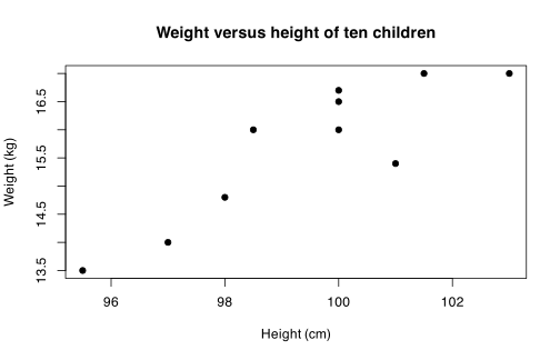
3.6- Make a scatter plot of Weight as a function of Height. Remember to add a title to your graph and to label your axes.
3.1- Use c() for every variable (Section 3.2.2.1), wrapped in factor() for the qualitative ones (Gender, ZEP, Section 3.2.2.5); names stay a character vector. Following the work strategy of Section 3.1.3, type these lines in a script and send them to the console. (Erratum: the preamble’s list of types should read “quantitative, ordinal or qualitative”.)
Individuals <- c("Edward", "Cynthia", "Eugene", "Elizabeth", "Patrick",
                 "John", "Albert", "Lawrence", "Joseph", "Leo")
Gender <- factor(c("G", "G", "B", "G", "B", "B", "B", "B", "B", "B"))
ZEP    <- factor(c("Y", "Y", "Y", "Y", "N", "Y", "N", "Y", "Y", "Y"))
Weight <- c(16, 14, 13.5, 15.4, 16.5, 16, 17, 14.8, 17, 16.7)
Years  <- c(3, 3, 3, 4, 3, 4, 3, 3, 4, 3)
Months <- c(5, 10, 5, 0, 8, 0, 11, 9, 1, 3)
Height <- c(100, 97, 95.5, 101, 100, 98.5, 103, 98, 101.5, 100)
Gender
[1] G G B G B B B B B B
Levels: B G
3.2- Only the quantitative variables have a mean: 15.69 kg for weight, 99.45 cm for height and 3.73 years for age (years plus months/12); a mean of a factor such as Gender is meaningless and R returns NA.
mean(Weight)
mean(Height)
mean(Years + Months/12)
mean(Gender)
[1] 15.69
[1] 99.45
[1] 3.733333
[1] NA
Warning message:
In mean.default(Gender) : argument is not numeric or logical: returning NA
3.3- BMI is weight in kg divided by the square of height in metres, so the heights must first be divided by 100; the children’s BMIs range from 14.8 to 16.7 kg/m\(^2\).
BMI <- Weight / (Height/100)^2
round(BMI, 2)
[1] 16.00 14.88 14.80 15.10 16.50 16.49 16.02 15.41 16.50 16.70
3.4- An individual × variable table, i.e. a data.frame (Section 3.2.2.4), since it holds columns of different types (character, factors, numerics) with one row per child.
Children <- data.frame(Individuals, Gender, ZEP, Weight, Years, Months,
                       Height, BMI)
str(Children)
'data.frame':	10 obs. of  8 variables:
 $ Individuals: chr  "Edward" "Cynthia" "Eugene" "Elizabeth" ...
 $ Gender     : Factor w/ 2 levels "B","G": 2 2 1 2 1 1 1 1 1 1
 $ ZEP        : Factor w/ 2 levels "N","Y": 2 2 2 2 1 2 1 2 2 2
 $ Weight     : num  16 14 13.5 15.4 16.5 16 17 14.8 17 16.7
 $ Years      : num  3 3 3 4 3 4 3 3 4 3
 $ Months     : num  5 10 5 0 8 0 11 9 1 3
 $ Height     : num  100 97 95.5 101 100 ...
 $ BMI        : num  16 14.9 14.8 15.1 16.5 ...
3.5- Type help(plot) or ?plot (Section 3.1.3); the page documents the generic plot(x, y, ...), lists under ... the common arguments type, main, sub, xlab, ylab and asp, points to ?par for graphical parameters, and example(plot) runs its examples.
3.6- Pass Height as x and Weight as y, with main, xlab and ylab for the title and axis labels; the plot shows weight rising roughly with height.
plot(Height, Weight, pch = 19, main = "Weight versus height of ten children",
     xlab = "Height (cm)", ylab = "Weight (kg)")
Importing, exporting and producing data
Exercises 4.1–4.7
Name the three main R functions to import data from an ASCII text file.
read.table() (rectangular data tables), read.ftable() (contingency tables) and scan() (the flexible, low-level reader for every other layout); see Table 4.1.
One of the usual data reading functions takes the following arguments: header, sep, dec, row.names, skip, nrows. Explain their purpose. Give an example of a value each argument can take.
The function is read.table() (Table 4.2):
| Argument | Purpose | Example |
|---|---|---|
header | whether the first line holds the variable names | TRUE |
sep | field separator on each line | "\t", " " |
dec | decimal mark of the numbers | "," |
row.names | column (number or name) giving the individuals’ names | 1 |
skip | number of lines to skip at the top of the file before reading | 5 |
nrows | maximum number of rows (individuals) to read | 100 |
For instance, the first three individuals of the book’s file (decimal comma, space separator):
x <- read.table("http://www.biostatisticien.eu/springeR/Intima_Media_Thickness.txt",
                header = TRUE, sep = " ", dec = ",", skip = 0, nrows = 3)
x
  GENDER AGE height weight tobacco packyear SPORT measure alcohol
1      1  33    170     70       1        1     0    0.52       1
2      2  33    177     67       2       20     0    0.42       1
3      2  53    164     63       1       30     0    0.65       0
What is the purpose of the function readLines()?
readLines() reads a file line by line as raw character strings, so its first few lines (argument n) show how the file is laid out and hence which read.table() arguments are needed (Section 4.1.1):
readLines("http://www.biostatisticien.eu/springeR/Intima_Media_Thickness.txt", n = 3)
[1] "GENDER AGE height weight tobacco packyear SPORT measure alcohol"
[2] "1 33 170 70 1 1 0 0,52 1"
[3] "2 33 177 67 2 20 0 0,42 1"
Here the header line, the space separator and the decimal comma are visible at once.
What is the purpose of the function fix()?
fix(X) opens the data.frame or matrix X in R’s mini spreadsheet so its values (and variable names) can be viewed and edited by hand; the modified object is saved back under the same name when the window is closed (Sections 4.1.2 and 4.3.3). Unlike View(), it allows editing, and unlike edit(), it needs no reassignment.
Give the specificities of the functions read.csv(), read.csv2(), read.delim() and read.delim2().
All four are read.table() with header = TRUE and preset separator and decimal mark (Section 4.1.1):
| Function | sep | dec |
|---|---|---|
read.csv() | "," | "." |
read.csv2() | ";" | "," |
read.delim() | "\t" (tab) | "." |
read.delim2() | "\t" (tab) | "," |
What is the purpose of the function read.ftable()?
read.ftable() reads a contingency table stored as a “flat” table in a text file (when only counts, not the individual data, are available) and returns an object of class ftable (Section 4.1.1):
tab <- read.ftable(url("http://www.biostatisticien.eu/springeR/Intima_ftable-en.txt"))
tab
                     alcohol nondrinker occasional drinker regular drinker
GENDER tobacco
M      non-smoker                     6                 19               7
       former smoker                  0                  9               0
       smoker                         1                  6               5
F      non-smoker                    12                 26               2
       former smoker                  3                  5               1
       smoker                         1                  6               1
Under R 4.5 the bare URL string makes read.ftable() fail when closing the connection, hence the url() wrapper.
What is the difference between the functions scan() and read.table()?
read.table() reads a rectangular file into a data.frame (one column per variable, with names, separators and types handled for you), whereas scan() reads the file as a stream of values into a vector (or a list, via what), ignoring the table structure; it is lower-level, faster and more flexible (what, skip, nlines, sep), so it handles irregular files that read.table() cannot (Table 4.1):
cat("a b\n1 2\n3 4\n", file = f <- tempfile())
scan(f, skip = 1)
read.table(f, header = TRUE)
Read 4 items
[1] 1 2 3 4
  a b
1 1 2
2 3 4
Exercises 4.8–4.14
Explain how you would import data from an Excel spreadsheet. Give details.
Three routes (Section 4.1.2):
- Copy-paste: select the data range in Excel, copy it (CTRL+C / COMMAND+C), then read the clipboard with
x <- read.table(file("clipboard"), sep = "\t", header = TRUE, dec = ",")(Excel puts tab-separated text on the clipboard; on macOS usepipe("pbpaste")instead offile("clipboard")). If the range holds formulae or hidden characters, first paste-special the values into a new sheet. - Intermediate ASCII file: in Excel, File / Save as … with type “Text (tab-separated) (*.txt)”, then use
read.delim()(orread.delim2()for a decimal comma). - A dedicated package reading
.xls/.xlsxdirectly:read_excel()fromreadxl, which needs no external software but reads local files only. The authors’ companion solution usesread.xls()fromgdata(Section 4.1.2.3), but that Perl-based function was removed ingdata3.0.
library(readxl)
f <- tempfile(fileext = ".xls")
download.file("http://www.biostatisticien.eu/springeR/Intima_Media_Thickness.xls",
              f, mode = "wb", quiet = TRUE)
d <- as.data.frame(read_excel(f))    # sheet = 1 by default
head(d, 3)
  GENDER AGE height weight tobacco packyear SPORT measure alcohol
1      1  33    170     70       1        1     0    0.52       1
2      2  33    177     67       2       20     0    0.42       1
3      2  53    164     63       1       30     0    0.65       0
Which package includes several functions to import data from commercial statistical software?
foreign: read.spss() (SPSS, .sav), read.mtp() (Minitab, .mtp), read.xport() (SAS XPORT, .xpt), among others (Table 4.3; Matlab files need readMat() from R.matlab):
library(foreign)
b <- read.spss("http://www.biostatisticien.eu/springeR/bmichild.sav", to.data.frame = TRUE)
head(b, 3)
  SEXE zep poids an mois taille
1    F   O  16.0  3    5  100.0
2    F   O  14.0  3   10   97.0
3    G   O  13.5  3    5   95.5
When reading a large data file, which argument to the function read.table() can speed up the reading?
colClasses, which declares the type of each column (e.g. colClasses = rep("character", 3)) so that R does not have to scan the whole file to infer them; in Section 4.1.4 this cuts the reading of dbsnp123.dat from about 5 minutes to 14 seconds. Giving nrows (even a mild over-estimate) also helps memory allocation.
Which R function should be used to write to a file a data set contained in a data.frame? Which other function do you know?
write.table() (Section 4.2.1); the other one is write(), meant for vectors and matrices (argument ncolumns, and it writes the transpose of a matrix). The wrappers write.csv() / write.csv2() are write.table() with CSV presets.
X <- data.frame(Weight = c(80, 90, 75), Height = c(182, 190, 160))
f <- tempfile(fileext = ".txt")
write.table(X, file = f, sep = "\t", row.names = FALSE)
readLines(f)
[1] "\"Weight\"\t\"Height\"" "80\t182"                "90\t190"
[4] "75\t160"
Name the four basic functions to create a vector.
c(), seq(), ":"() and rep() (Section 4.3.1).
Explain how the function seq() can be used to get the following vector:
[1] 1.0 1.1 1.2 1.3 1.4 1.5 1.6 1.7 1.8 1.9 2.0
Give the endpoints and either the step by or the number of values length:
seq(from = 1, to = 2, by = 0.1)
seq(1, 2, length = 11)
[1] 1.0 1.1 1.2 1.3 1.4 1.5 1.6 1.7 1.8 1.9 2.0
[1] 1.0 1.1 1.2 1.3 1.4 1.5 1.6 1.7 1.8 1.9 2.0
Give the shortest R instruction which outputs the following vector:
1 1 2 2 3 3
rep(1:3, e = 2), i.e. rep(1:3, each = 2) with the argument name partially matched:
rep(1:3, e = 2)
[1] 1 1 2 2 3 3
Exercises 4.15–4.16
Give the shortest R instruction which outputs the following vector:
1 2 3 1 2 3
rep(1:3, 2), since the second argument times repeats the whole vector:
rep(1:3, 2)
[1] 1 2 3 1 2 3
Name two R functions which can be used to enter data by hand in a mini spreadsheet.
data.entry() (variables of possibly different lengths, created directly in the workspace) and de() (e.g. X <- as.data.frame(de("")) for an individuals \(\times\) variables table); see Section 4.3.3. fix() then edits an existing data.frame in the same spreadsheet. These open an interactive window, so they cannot be run in a script.
Worksheet 4.W.A.1 — Entering data from a hard copy - Fever blisters
Worksheet 4.W.A.1 — Entering data from a hard copy — Fever blisters
Fever blisters: Thirty patients have been randomly assigned to one of five treatments against fever blisters, including one placebo (there are six patients in each treatment group). For each patient, the number of days between the apparition of the first blisters and complete healing has been recorded.
| trt1 (placebo) | trt2 | trt3 | trt4 | trt5 |
|---|---|---|---|---|
| 5 | 4 | 6 | 7 | 9 |
| 8 | 6 | 4 | 4 | 3 |
| 7 | 6 | 4 | 6 | 5 |
| 7 | 3 | 5 | 6 | 7 |
| 10 | 5 | 4 | 3 | 7 |
| 8 | 6 | 3 | 5 | 6 |
We would like to know whether there is a difference between the treatments, by comparing the mean healing time in each independent random sample (treatment group). The relevant statistical method is called ANOVA; we shall present it in Chapter 15. In this practical, we shall simply see how to enter these data in R to compute the sample mean for each treatment.
4.1- Enter the data in R directly, using the function de().
4.2- Use the function attach(), then the function mean() to compute the mean for each treatment.
4.3- Compute the means of all treatments simultaneously thanks to the function colMeans().
4.4- Use the function write.table() to save your data.frame in a file called blisters.txt.
4.5- Open your file in a text editor and check that there was no problem.
4.6- Use the function rm() to delete all the R objects you have created in your work environment.
4.7- Import the file blisters.txt with the function read.table() and display the data.
4.1- Type blisters <- as.data.frame(de("")) (Section 4.3.3): in the spreadsheet window, click each header cell to rename the columns trt1, …, trt5 and set them to numeric, type the six values of each column, then close the window. de() needs a graphical device, so it cannot run in a script; the non-interactive instruction below builds the same data frame, and is what the remaining answers use.
blisters <- data.frame(trt1 = c(5, 8, 7, 7, 10, 8), trt2 = c(4, 6, 6, 3, 5, 6),
                       trt3 = c(6, 4, 4, 5, 4, 3), trt4 = c(7, 4, 6, 6, 3, 5),
                       trt5 = c(9, 3, 5, 7, 7, 6))
blisters
  trt1 trt2 trt3 trt4 trt5
1    5    4    6    7    9
2    8    6    4    4    3
3    7    6    4    6    5
4    7    3    5    6    7
5   10    5    4    3    7
6    8    6    3    5    6
4.2- After attach() the columns are visible as ordinary variables, so mean() works on each by name:
attach(blisters)
c(mean(trt1), mean(trt2), mean(trt3), mean(trt4), mean(trt5))
detach(blisters)
[1] 7.500000 5.000000 4.333333 5.166667 6.166667
4.3- colMeans() gives all five means in one call, with names:
colMeans(blisters)
    trt1     trt2     trt3     trt4     trt5
7.500000 5.000000 4.333333 5.166667 6.166667
The placebo has the longest mean healing time (7.5 days) and trt3 the shortest (4.33 days); Chapter 15 tests whether these differences are significant.
4.4- The file is written to the working directory (getwd()):
write.table(blisters, file = "blisters.txt")
4.5- Any text editor shows the contents; here they are printed from R with readLines():
cat(readLines("blisters.txt"), sep = "\n")
"trt1" "trt2" "trt3" "trt4" "trt5"
"1" 5 4 6 7 9
"2" 8 6 4 4 3
"3" 7 6 4 6 5
"4" 7 3 5 6 7
"5" 10 5 4 3 7
"6" 8 6 3 5 6
The file is correct. The row names are written as a first column, which is why the header line has one field less than the data lines.
4.6- ls() lists every object, so the call below removes them all; the empty ls() afterwards confirms it:
rm(list = ls())
ls()
character(0)
4.7- Read the file back with its header:
blisters <- read.table("blisters.txt", header = TRUE)
blisters
  trt1 trt2 trt3 trt4 trt5
1    5    4    6    7    9
2    8    6    4    4    3
3    7    6    4    6    5
4    7    3    5    6    7
5   10    5    4    3    7
6    8    6    3    5    6
Since the header line is one field short, read.table() reads the first column as row names, and we get back the same data frame we saved.
Worksheet 4.W.A.2 — Entering data from a hard copy - Risk factors for atherosclerosis
Worksheet 4.W.A.2 — Entering data from a hard copy — Risk factors for atherosclerosis
Risk factors for atherosclerosis: As part of a study on risk factors for atherosclerosis, data were collected and are summed up in this contingency table:
| GENDER | tobacco | nondrinker | occasional-drinker | regular-drinker |
|---|---|---|---|---|
| M | non-smoker | 6 | 19 | 7 |
| M | former smoker | 0 | 9 | 0 |
| M | smoker | 1 | 6 | 5 |
| F | non-smoker | 12 | 26 | 2 |
| F | former smoker | 3 | 5 | 1 |
| F | smoker | 1 | 6 | 1 |
It would be interesting to know whether there is a dependence between smoking and drinking, according to gender. To enter these data in R, there are several steps.
4.1- Use the function scan() to get a matrix X of size \(6 \times 3\). This matrix will contain the data only.
4.2- Use the instruction class(X) <- "ftable" to specify that it is a contingency table.
4.3- Type the two instructions:
attributes(X)$col.vars <- list(alcohol=c("nondrinker",
            "occasional-drinker","regular-drinker"))
attributes(X)$row.vars <- list(GENDER=c("M","F"),tobacco=
               c("non-smoker","former smoker","smoker"))
4.4- Display the contingency table you have created.
4.5- Use the function write.ftable() to save the contingency table in a file called athero.txt.
4.6- Open the file in a text editor and check that there was no problem.
4.7- Use the function rm() to delete all the R objects you have created in your work environment.
4.8- Import the file athero.txt with the function read.table() and display the data.
4.1- Type X <- matrix(scan(), ncol = 3, byrow = TRUE) and enter the 18 counts row by row, ending with an empty line (Section 4.3.3); byrow = TRUE fills the matrix one table row at a time. Here the typed input is given to scan() through its text argument so that the code can be rerun:
X <- matrix(scan(text = "6 19 7  0 9 0  1 6 5  12 26 2  3 5 1  1 6 1"),
            ncol = 3, byrow = TRUE)
X
Read 18 items
     [,1] [,2] [,3]
[1,]    6   19    7
[2,]    0    9    0
[3,]    1    6    5
[4,]   12   26    2
[5,]    3    5    1
[6,]    1    6    1
4.2- and 4.3- These two steps give X its class and the two attributes (row.vars, col.vars) that print.ftable() needs to label the table:
class(X) <- "ftable"
attributes(X)$col.vars <- list(alcohol=c("nondrinker",
            "occasional-drinker","regular-drinker"))
attributes(X)$row.vars <- list(GENDER=c("M","F"),tobacco=
               c("non-smoker","former smoker","smoker"))
4.4- Typing the object’s name prints it as a flat table:
X
                     alcohol nondrinker occasional-drinker regular-drinker
GENDER tobacco
M      non-smoker                     6                 19               7
       former smoker                  0                  9               0
       smoker                         1                  6               5
F      non-smoker                    12                 26               2
       former smoker                  3                  5               1
       smoker                         1                  6               1
It matches the printed table.
4.5- The table is written in the working directory:
write.ftable(X, file = "athero.txt")
4.6- Here the file is printed from R:
cat(readLines("athero.txt"), sep = "\n")
                         "alcohol" "nondrinker" "occasional-drinker" "regular-drinker"
"GENDER" "tobacco"
"M"      "non-smoker"                         6                   19                 7
         "former smoker"                      0                    9                 0
         "smoker"                             1                    6                 5
"F"      "non-smoker"                        12                   26                 2
         "former smoker"                      3                    5                 1
         "smoker"                             1                    6                 1
The file holds the flat table with every label quoted. The GENDER label is written only on the first row of each block, so the lines do not all have the same number of fields.
4.7- Remove every object; the empty ls() confirms it:
rm(list = ls())
ls()
character(0)
4.8- read.table() fails on this file because its lines have different numbers of fields. This is an erratum in the book: the intended import function is read.ftable() (Section 4.1.1.2), which reads the labels back from the file’s own header:
try(read.table("athero.txt"))
X <- read.ftable("athero.txt")
X
Error in scan(file = file, what = what, sep = sep, quote = quote, dec = dec,  :
  line 1 did not have 5 elements
                     alcohol nondrinker occasional-drinker regular-drinker
GENDER tobacco
M      non-smoker                     6                 19               7
       former smoker                  0                  9               0
       smoker                         1                  6               5
F      non-smoker                    12                 26               2
       former smoker                  3                  5               1
       smoker                         1                  6               1
We get back the contingency table of 4.4 exactly.
Worksheet 4.W.B — Importing from other software
Worksheet 4.W.B — Importing from other software — BMI of children
During a study of BMI (Body Mass Index) of children, a team of statisticians collected data in different formats. As an exercise, we are going to read these various formats. There are several files called bmichild, but with different file extensions.
4.1- Import the file bmichild.xls into a data.frame called bmi.XLS.
4.2- Import the file bmichild.xpt into a data.frame called bmi.SAS.
4.3- Import the file bmichild.sav into a data.frame called bmi.SPSS.
4.4- Import the file bmichild.mat into a data.frame called bmi.MAT. The procedure is trickier for this file, so here are detailed instructions:
x <- readMat("bmichild.mat")
class(x) # x is a list
x        # you can see that the data are in $bmi[,,1]
x <- x$bmi[,,1]
  # Note that the elements of GENDER and zep
  # are recorded in a list.
x$GENDER
class(x$GENDER) <- "character"
x$GENDER
class(x$zep) <- "character"
bmi.MAT <- as.data.frame(x)
4.5- To check that there was no problem during importation, use the function summary() on all these data.frames. This will display a few numerical summaries.
4.6- All these data.frames are identical. Save one of them in a file called bmichild.txt.
4.1- The book’s read.xls() (package gdata, Section 4.1.2.3) was removed from gdata 3.0, so use read_excel() from readxl, which reads only local files, hence the download.file() first.
library(readxl)
url <- "http://www.biostatisticien.eu/springeR/"
download.file(paste0(url, "bmichild.xls"), "bmichild.xls", mode = "wb", quiet = TRUE)
bmi.XLS <- as.data.frame(read_excel("bmichild.xls"))
head(bmi.XLS, 3)
  GENDER zep weight year month height
1      F   Y   16.0    3     5  100.0
2      F   Y   14.0    3    10   97.0
3      M   Y   13.5    3     5   95.5
4.2- read.xport() from foreign (Table 4.3). As the Warning in Section 4.1.3 says, it cannot read from a URL, so the file is downloaded first. lookup.xport() gives the variable names.
library(foreign)
download.file(paste0(url, "bmichild.xpt"), "bmichild.xpt", mode = "wb", quiet = TRUE)
lookup.xport("bmichild.xpt")$SAS$name
bmi.SAS <- read.xport("bmichild.xpt")
head(bmi.SAS, 3)
[1] "SEXE"   "ZEP"    "POIDS"  "AN"     "MOIS"   "TAILLE"
  SEXE ZEP POIDS AN MOIS TAILLE
1    F   O  16.0  3    5  100.0
2    F   O  14.0  3   10   97.0
3    G   O  13.5  3    5   95.5
The .xpt, .sav and .mat files come from the French edition of the book. Their variables are SEXE (gender, coded F/G for fille/garçon), ZEP (priority-education zone, coded O/N for oui/non), POIDS (weight), AN and MOIS (age in years and months) and TAILLE (height). So G stands for M and O stands for Y.
4.3- read.spss() from foreign reads directly from the URL. The argument to.data.frame = TRUE returns a data.frame instead of the default list.
bmi.SPSS <- read.spss(paste0(url, "bmichild.sav"), to.data.frame = TRUE)
head(bmi.SPSS, 3)
  SEXE zep poids an mois taille
1    F   O  16.0  3    5  100.0
2    F   O  14.0  3   10   97.0
3    G   O  13.5  3    5   95.5
4.4- readMat() from R.matlab (Table 4.3; installed from CRAN for this run). This part of the book’s instructions no longer works as printed. The served file stores the data in $imc (with French names SEXE and zep), not $bmi (GENDER and zep). Also, each SEXE and zep entry is a list holding a \(1 \times 1\) matrix. In current R, class(x$SEXE) <- "character" deparses these entries into strings like "list(\"F\")", so unlist() is used to flatten them.
library(R.matlab)
download.file(paste0(url, "bmichild.mat"), "bmichild.mat", mode = "wb", quiet = TRUE)
x <- readMat("bmichild.mat")
class(x)
names(x)
x <- x$imc[,,1]
names(x)
x$SEXE[1:2]
x$SEXE <- unlist(x$SEXE)
x$zep <- unlist(x$zep)
bmi.MAT <- as.data.frame(x)
head(bmi.MAT, 3)
[1] "list"
[1] "imc"
[1] "SEXE"   "zep"    "poids"  "an"     "mois"   "taille"
[[1]]
[[1]][[1]]
     [,1]
[1,] "F"


[[2]]
[[2]][[1]]
     [,1]
[1,] "F"


  SEXE zep poids an mois taille
1    F   O  16.0  3    5  100.0
2    F   O  14.0  3   10   97.0
3    G   O  13.5  3    5   95.5
4.5- Apply summary() to all four data.frames. The two coded columns are converted to factors first, so that summary() counts their levels.
bmi <- list(XLS = bmi.XLS, SAS = bmi.SAS, SPSS = bmi.SPSS, MAT = bmi.MAT)
bmi <- lapply(bmi, function(d) {d[1:2] <- lapply(d[1:2], factor); d})
lapply(bmi, summary)
$XLS
 GENDER zep         weight           year           month
 F:71   N: 41   Min.   :10.50   Min.   :3.000   Min.   : 0.000
 M:81   Y:111   1st Qu.:15.00   1st Qu.:3.000   1st Qu.: 3.000
                Median :16.00   Median :3.000   Median : 6.000
                Mean   :16.28   Mean   :3.303   Mean   : 5.618
                3rd Qu.:17.50   3rd Qu.:4.000   3rd Qu.: 9.000
                Max.   :22.80   Max.   :4.000   Max.   :11.000
     height
 Min.   : 88.5
 1st Qu.: 98.0
 Median :101.0
 Mean   :100.7
 3rd Qu.:103.6
 Max.   :111.5

## ... $SAS, $SPSS and $MAT truncated: identical numbers, printed under
## the French names and codes (F:71 G:81, N:41 O:111)
The truncated summaries are easiest to compare side by side:
sapply(bmi, function(d) c(table(d[[1]]), table(d[[2]]), colMeans(d[3:6])))
              XLS        SAS       SPSS        MAT
F       71.000000  71.000000  71.000000  71.000000
M       81.000000  81.000000  81.000000  81.000000
N       41.000000  41.000000  41.000000  41.000000
Y      111.000000 111.000000 111.000000 111.000000
weight  16.280263  16.280263  16.280263  16.280263
year     3.302632   3.302632   3.302632   3.302632
month    5.618421   5.618421   5.618421   5.618421
height 100.748026 100.748026 100.748026 100.748026
All four imports agree: 152 children, 71 girls and 81 boys, 111 in a ZEP, weights from 10.5 to 22.8 kg and heights from 88.5 to 111.5 cm, so no problem occurred during importation.
4.6- write.table() (Section 4.2.1) saves the data. Here bmi.XLS is saved, with tab separators and no row names.
write.table(bmi.XLS, file = "bmichild.txt", sep = "\t", quote = FALSE,
            row.names = FALSE)
readLines("bmichild.txt", n = 3)
[1] "GENDER\tzep\tweight\tyear\tmonth\theight"
[2] "F\tY\t16\t3\t5\t100"
[3] "F\tY\t14\t3\t10\t97"
Worksheet 4.W.C — Importing more complex data files
Worksheet 4.W.C — Importing more complex data files
Statisticians often encounter data files in non-standard formats. This section therefore provides training in reading several non-standard files on which we wish to perform statistical analysis.
4.1- Import the file raf98.gra into the most relevant structure. To this end, you will need to read the associated file geoidformat.txt which describes the file format.
4.2- Import the file Infarction.xls into a data.frame. Make sure you handle missing values correctly.
4.3- The file nutrition_elderly.txt contains thirteen variables measured on 226 individuals. Import the file into a data.frame (hint: use the functions t() and as.data.frame()).
4.4- The file Birth_weight.txt contains ten variables measured on 189 individuals. Import it into a data.frame, which will contain the names of the variables as well as the names of the individuals (these are available in the column Id). Remember that you can use the online help!
4.1- The file is a grid, so the natural structure is a \(381 \times 421\) matrix of geoid heights (rows = latitudes from north to south, columns = longitudes from west to east), read with scan() (Section 4.1.1.3) since the values are not laid out as a rectangular table. According to geoidformat.txt, the first three lines hold the bounds and steps, and the values then follow row by row regardless of line breaks (52 lines of 8 plus one line of 5 per latitude, i.e. \(52 \times 8 + 5 = 421\)).
url <- "http://www.biostatisticien.eu/springeR/"
header <- scan(paste0(url, "raf98.gra"), nlines = 3)
z <- scan(paste0(url, "raf98.gra"), skip = 3)
lat <- seq(header[2], header[1], by = -header[5])   # north to south
long <- seq(header[3], header[4], by = header[6])   # west to east
raf98 <- matrix(z, nrow = length(lat), ncol = length(long), byrow = TRUE,
                dimnames = list(round(lat, 3), round(long, 3)))
header
dim(raf98)
raf98[1:3, 1:4]
range(raf98)
Read 6 items
Read 160401 items
[1] 42.00000000 51.50000000 -5.50000000  8.50000000  0.02500000  0.03333333
[1] 381 421
          -5.5  -5.467  -5.433    -5.4
51.5   53.3573 53.3569 53.3546 53.3481
51.475 53.3284 53.3277 53.3259 53.3209
51.45  53.3056 53.3023 53.2990 53.2940
[1] 41.8493 55.4308
The \(160401 = 381 \times 421\) values fill the grid exactly, and the geoid heights over France range from about 41.8 m to 55.4 m.
4.2- The spreadsheet codes missing values as a dot ., so declare it with na = "." (the equivalent of na.strings = "." in read.table()). We use read_excel() from readxl, which needs a local copy of the file. The authors’ companion solution uses read.xls() from gdata (Section 4.1.2.3), which was removed in gdata 3.0; the missing-value handling is the same.
library(readxl)
tmp <- tempfile(fileext = ".xls")
download.file("http://www.biostatisticien.eu/springeR/Infarction.xls", tmp,
              mode = "wb", quiet = TRUE)
infarct <- as.data.frame(read_excel(tmp, na = "."))
str(infarct)
colSums(is.na(infarct))
'data.frame':	449 obs. of  10 variables:
 $ NUMBER : num  1 2 3 4 5 6 7 8 9 10 ...
 $ INFARCT: num  0 0 0 0 0 0 0 0 0 0 ...
 $ CO     : num  0 0 0 0 0 0 0 0 0 0 ...
 $ TOBACCO: num  0 0 0 0 0 0 0 0 0 0 ...
 $ AGE    : num  47 17 35 82 50 31 60 30 44 38 ...
 $ WEIGHT : num  48 NA 53 78 52 47 60 75 68 NA ...
 $ HEIGHT : num  173 162 163 157 172 184 169 174 164 167 ...
 $ BMI    : num  16 NA 19.9 31.6 17.6 ...
 $ ATCD   : num  0 0 0 0 NA 0 0 0 0 0 ...
 $ HTA    : num  0 0 0 0 0 0 0 0 0 0 ...
 NUMBER INFARCT      CO TOBACCO     AGE  WEIGHT  HEIGHT     BMI    ATCD     HTA
      0       0       0       0       0      12       0      12       7       0
All ten variables are now numeric, with 12 missing weights (hence 12 missing BMIs) and 7 missing ATCD; without na = "." the columns WEIGHT, BMI and ATCD would have been read as character strings.
4.3- The file stores one variable per line (name followed by its 226 values), so read it with the names as row names, then transpose with t() and convert with as.data.frame().
url <- "http://www.biostatisticien.eu/springeR/"
tmp <- read.table(paste0(url, "nutrition_elderly.txt"), row.names = 1)
dim(tmp)
nutri <- as.data.frame(t(tmp))
rownames(nutri) <- NULL
dim(nutri)
head(nutri, 3)
[1]  13 226
[1] 226  13
  gender situation tea coffee height weight age mea fish raw_fruits
1      2         1   0      0    151     58  72   4    3          1
2      2         1   1      1    162     60  68   5    2          5
3      2         1   0      4    162     75  78   3    1          5
  cooked_fruits_veg chocol fat
1                 4      5   6
2                 5      1   4
3                 2      5   4
The data.frame has the expected 226 individuals (rows) and 13 variables (columns).
4.4- readLines() shows the traps: the header is space-separated while the data are separated by ;, and (looking at the end of the file) a line of dashes follows the 189 records. So read the names with scan(), then the data with sep = ";", skip = 1, nrows = 189, and use row.names = "ID" to turn the identifier column into row names (the column is printed Id in the book but is called ID in the file).
url <- "http://www.biostatisticien.eu/springeR/"
readLines(paste0(url, "Birth_weight.txt"), n = 3)
nm <- scan(paste0(url, "Birth_weight.txt"), what = "", nlines = 1)
birth <- read.table(paste0(url, "Birth_weight.txt"), sep = ";", skip = 1,
                    nrows = 189, col.names = nm, row.names = "ID")
dim(birth)
head(birth, 3)
[1] "\"ID\" \"AGE\" \"LWT\" \"RACE\" \"SMOKE\" \"PTL\" \"HT\" \"UI\" \"FVT\" \"BWT\" \"LOW\""
[2] "85;19;182;2;0;0;0;1;0;2523;0"
[3] "86;33;155;3;0;0;0;0;3;2551;0"
Read 11 items
[1] 189  10
   AGE LWT RACE SMOKE PTL HT UI FVT  BWT LOW
85  19 182    2     0   0  0  1   0 2523   0
86  33 155    3     0   0  0  0   3 2551   0
87  20 105    1     1   0  0  0   1 2557   0
The result has the 189 individuals named by their ID and the ten variables named from the header; without nrows = 189, read.table() stops with “line 193 did not have 11 elements” because of the trailing dashes.
Data manipulation, functions
Exercises 5.1–5.7
What is the output of this instruction: c(1,4)*c(2,3)?
The output is the vector 2 12: * multiplies term by term, it is not a scalar product.
c(1,4)*c(2,3)
[1] 2 12
What is the output of this instruction: matrix(1:2,ncol=2,nrow=2)?
A \(2\times 2\) matrix whose two columns both equal 1:2, because the vector is filled column by column and recycled.
matrix(1:2,ncol=2,nrow=2)
     [,1] [,2]
[1,]    1    1
[2,]    2    2
How can you retrieve the names of rows and columns of a data.frame?
With rownames() and colnames() (or names() for the columns), or both at once with dimnames().
df <- data.frame(a = 1:2, b = 3:4, row.names = c("r1", "r2"))
rownames(df); colnames(df)
[1] "r1" "r2"
[1] "a" "b"
Give the instruction to merge these two tables:
> X
      Gender Weight
Jack       M     80
Julia      F     60
> Y
        Eyes Height
Jack    Blue    180
Julia  Green    160
merge(X, Y, by = "row.names") merges the two tables on their common row names (cbind(X, Y) also works here because the rows are already in the same order).
X <- data.frame(Gender = c("M", "F"), Weight = c(80, 60),
                row.names = c("Jack", "Julia"))
Y <- data.frame(Eyes = c("Blue", "Green"), Height = c(180, 160),
                row.names = c("Jack", "Julia"))
merge(X, Y, by = "row.names")
  Row.names Gender Weight  Eyes Height
1      Jack      M     80  Blue    180
2     Julia      F     60 Green    160
Give the instruction to calculate the product of all the elements (respectively: of all the elements of each column) of a numerical matrix X.
prod(X) gives the product of all the elements, and apply(X, 2, prod) the product of each column.
X <- matrix(1:6, nrow = 2)
prod(X)
apply(X, 2, prod)
[1] 720
[1]  2 12 30
What is the output of this instruction: vec<-c(2,4,6,8,3);vec[2];vec[-2]?
vec[2] is the second element, 4, and vec[-2] is the vector without its second element.
vec<-c(2,4,6,8,3);vec[2];vec[-2]
[1] 4
[1] 2 6 8 3
The height and weight of several men were measured. The measurements are stored in the vectors weight and height. Give the R instruction to get the weight of the men whose height is greater than 180 cm.
weight[height > 180]: the logical vector indexes weight. With some illustrative values:
weight <- c(70, 85, 92, 64); height <- c(175, 183, 190, 168)
weight[height > 180]
[1] 85 92
Exercises 5.8–5.14
What is the output of this instruction Mat<-matrix(1:12,nrow=4,byrow=TRUE);Mat[3,];Mat[2,2:3]?
Mat[3,] is the third row 7 8 9 and Mat[2,2:3] is 5 6, since byrow=TRUE fills the rows 1:3, 4:6, 7:9, 10:12.
Mat<-matrix(1:12,nrow=4,byrow=TRUE);Mat[3,];Mat[2,2:3]
[1] 7 8 9
[1] 5 6
How could you replace the fourth component of the following list with 1:10?
L<-list(12,c(34,67),Mat,1:15,list(10,11))
L[[4]] <- 1:10 (the double bracket addresses the component itself; Mat is the matrix of Exercise 5.8).
L<-list(12,c(34,67),Mat,1:15,list(10,11))
L[[4]] <- 1:10
L[[4]]
[1] 1 2 3 4 5 6 7 8 9 10
What is the output of this instruction: L[[2]][2]?
67: L[[2]] is the vector c(34,67) and [2] takes its second element.
L[[2]][2]
[1] 67
Give the R instruction which outputs the weights and heights of all women in the following table (you can use the function attach()):
| weight | height | gender | |
|---|---|---|---|
| 1 | 79 | 163 | M |
| 2 | 90 | 163 | F |
| 3 | 87 | 198 | M |
| 4 | 63 | 164 | F |
| 5 | 90 | 168 | F |
| 6 | 71 | 178 | F |
| 7 | 58 | 191 | M |
| 8 | 80 | 194 | F |
| 9 | 91 | 185 | F |
| 10 | 89 | 176 | M |
subset(X, gender = “F”, select = c(weight, height))=, or equivalently attach(X); X[gender = “F”, c(“weight”, “height”)]; detach(X)= (in this session subset() avoids attach()’s masking clash with the vectors weight, height of Exercise 5.7).
X <- data.frame(weight = c(79, 90, 87, 63, 90, 71, 58, 80, 91, 89),
                height = c(163, 163, 198, 164, 168, 178, 191, 194, 185, 176),
                gender = c("M", "F", "M", "F", "F", "F", "M", "F", "F", "M"))
subset(X, gender == "F", select = c(weight, height))
  weight height
2     90    163
4     63    164
5     90    168
6     71    178
8     80    194
9     91    185
What is the output of this instruction: (1:3)[any(c(T,F,T))]? And this one: (1:3)[all(c(T,F,T))]?
The first gives 1 2 3 (any() is TRUE, recycled over all indices) and the second integer(0) (all() is FALSE, so nothing is selected).
(1:3)[any(c(T,F,T))]
(1:3)[all(c(T,F,T))]
[1] 1 2 3
integer(0)
What is the output of this instruction: c(T,T,F) | c(F,T,F)? And this one: c(T,T,F) || c(F,T,F)?
| is term-wise and gives TRUE TRUE FALSE; || expects single values: in R 4.3.0 and later it throws an error on length-3 operands, whereas in the R version used by the book it compared only the first elements and returned TRUE. The authors’ companion solution gives TRUE for the second instruction; that is the pre-4.3.0 behaviour, reproduced today by c(T,T,F)[1] || c(F,T,F)[1].
c(T,T,F) | c(F,T,F)
c(T,T,F) || c(F,T,F)
[1]  TRUE  TRUE FALSE
Error in c(T, T, F) || c(F, T, F) :
  'length = 3' in coercion to 'logical(1)'
What is the output of this instruction: nchar(c("abcd","efgh"))?
4 4: nchar() is vectorised and counts the characters of each string.
nchar(c("abcd","efgh"))
[1] 4 4
Exercises 5.15–5.20
What is the output of this instruction?
paste(c("a","b"),c("c","d"),collapse="",sep="")
"acbd": sep""= first pastes term by term into "ac", "bd", then collapse""= joins these into one string.
paste(c("a","b"),c("c","d"),collapse="",sep="")
[1] "acbd"
What is the output of this instruction: strsplit(c("ab;cd"),";")?
A list with one component, the vector "ab" "cd": strsplit() always returns a list, one component per input string.
strsplit(c("ab;cd"),";")
[[1]]
[1] "ab" "cd"
What is the output of this instruction: substring("abcdef",3,c(2,4))?
The vector "" "cd": the string is recycled against last = c(2,4), and the sub-string from character 3 to character 2 is empty.
substring("abcdef",3,c(2,4))
[1] "" "cd"
How could you transform the upper case into lower case in the following vector?
c("Jack","Julia","William")
With tolower() (casefold(x, upper = FALSE) is equivalent).
tolower(c("Jack","Julia","William"))
[1] "jack" "julia" "william"
Which function is used to retrieve a date from a character string?
strptime(), whose format argument describes how the date is written in the string (as.Date() does the same for dates without a time).
strptime("24/09/2026", format = "%d/%m/%Y", tz = "UTC")
[1] "2026-09-24 UTC"
Can you explain why the second number of the last output is not equal to 36.21313?
> logp <- function(x) log(max(x,exp(1)))
> x <- -2.4
> delta <- 0.1
> (abs(x))^(4+delta)/(logp(abs(x)))^2
[1] 36.21313
> x <- seq(from=-2.8,to=-2,length=3)
> x
[1] -2.8 -2.4 -2.0
> (abs(x))^(4+delta)/(logp(abs(x)))^2
[1] 64.26795 34.15959 16.17594
Propose a solution to this problem.
max() is not vectorised: it returns the single largest value of all its arguments, here \(\max(2.8, 2.4, 2, e) = 2.8\), so every element is divided by \((\log 2.8)^2\) instead of its own \((\log \max(|x_i|, e))^2\). The fix is the term-wise maximum pmax().
logp <- function(x) log(max(x,exp(1)))
x <- seq(from=-2.8,to=-2,length=3); delta <- 0.1
logp(abs(x))
logp <- function(x) log(pmax(x, exp(1)))
(abs(x))^(4+delta)/(logp(abs(x)))^2
[1] 1.029619
[1] 64.26795 36.21313 17.14838
Worksheet 5.W.A — Manipulating a few data sets presented at the beginning of the book
Worksheet 5.W.A — Manipulating a few data sets presented at the beginning of the book — Manipulating various data sets
These files can be downloaded from the URL http://www.biostatisticien.eu/springeR/. Note that you can also append the file name at the end of this URL to download the file directly from R (e.g. http://www.biostatisticien.eu/springeR/nutrien1.xls).
Data set NE:
The data file nutrition_elderly.xls, described earlier in this book, is in fact the merge of two initial files, entered by different operators. We propose to reconstruct the file for the following cases. You will only use R, and will not edit the file by hand.
5.1- The individuals are initially listed separately in two files (nutrien1.xls and nutrien2.xls). Note that the variable names are in upper case in the first file, and in lower case in the second.
5.2- Some individuals are listed in both files (nutrien3.xls and nutrien4.xls). The variable names are identical.
5.3- Same question as 5.2, but errors have slipped in and you will need to detect the corresponding individuals, for example those with a weight greater than 200 kg (nutrien5.xls and nutrien6.xls).
5.4- The variables are split between two files (nutrien7.xls and nutrien8.xls), which contain the same individuals.
5.5- Same question as 5.4, but for one variable, too many values are missing. Remove that variable (nutrien9.xls and nutrien10.xls).
5.6- Same question as 5.4, but for one individual, too many values are missing. Remove that individual (nutrien11.xls and nutrien12.xls).
5.7- In the file nutrition_elderly.xls, how many people are vegetarians (no meat, no fish)?
File Intima_Media_Thickness.xls:
5.1- Add a column BMI to the data.frame, with the BMI of each individual in the data file.
5.2- Retrieve the thickness of intima for the people with a BMI>30.
5.3- Extract the “athletic” women.
5.4- Extract the “non-obese” people aged 50 or other (obese = BMI>30).
File bmichild.xls:
5.1- Add a column BMI.
5.2- Extract the children with a BMI < 15 and an age < 3.5= years.
5.3- How many such children are there?
File Birth_weight.xls:
5.1- Add a variable PTL1 (number of children born before term), with three modalities (where the third modality, coded 2, corresponds to “2 or more” pre-term births).
5.2- Same question with FVT (number of visits to a physician), to add FVT1.
5.3- Sort the file by increasing weight at birth (BWT).
5.4- Extract the individuals whose mothers are black or white and smoke.
Data set NE (all files are read straight from the book’s URL with read_excel() from readxl; the helper get.xls() is reused below).
5.1- Give both files the column names of nutrition_elderly.xls, then stack them with rbind() (Section 5.1.4.2); toupper()=/=tolower() alone is not enough because the second operator also typed vmeat and the target file uses raw_fruit.
library(readxl)
url <- "http://www.biostatisticien.eu/springeR/"
get.xls <- function(f) {
  tf <- tempfile(fileext = ".xls")
  download.file(paste0(url, f), tf, mode = "wb", quiet = TRUE)
  as.data.frame(read_excel(tf))
}
ne <- get.xls("nutrition_elderly.xls")
n1 <- get.xls("nutrien1.xls"); n2 <- get.xls("nutrien2.xls")
rbind(n1 = names(n1), n2 = names(n2), ne = names(ne))[, 8:11]
names(n1) <- names(n2) <- names(ne)
NE1 <- rbind(n1, n2)
dim(NE1)
all.equal(NE1, ne)
   [,1]    [,2]   [,3]         [,4]
n1 "MEAT"  "FISH" "RAW_FRUITS" "COOKED_FRUITS_VEG"
n2 "vmeat" "fish" "raw_fruits" "cooked_fruits_veg"
ne "meat"  "fish" "raw_fruit"  "cooked_fruit_veg"
[1] 226  13
[1] TRUE
The 109 + 117 rows rebuild nutrition_elderly.xls exactly.
5.2- merge(..., all = TRUE) on all the common columns (Section 5.1.4.2) is a full outer join, so each of the 5 individuals present in both files is kept once.
n3 <- get.xls("nutrien3.xls"); n4 <- get.xls("nutrien4.xls")
c(nrow(n3), nrow(n4))
intersect(n3$Subject, n4$Subject)
NE2 <- merge(n3, n4, all = TRUE)   # outer join on all 14 common columns
dim(NE2)
NE2 <- NE2[order(NE2$Subject), -1]; names(NE2) <- names(ne)
nrow(merge(NE2, ne))               # every reconstructed row is found in ne
[1] 112 119
[1]  51 137  85  30 156
[1] 226  14
[1] 226
The 112 + 119 - 5 = 226 individuals are exactly those of nutrition_elderly.xls (unique(rbind(n3, n4)) gives the same table).
5.3- The same merge now returns 227 rows, because one duplicated subject was typed differently; the printed rule “weight greater than 200 kg” finds nobody (the faulty weight is exactly 200, a small erratum), so we flag every value outside the coding of the data description (gender in {1, 2}, frequencies 0 to 5, fat 1 to 8) or physically implausible for elderly adults.
n5 <- get.xls("nutrien5.xls"); n6 <- get.xls("nutrien6.xls")
nrow(merge(n5, n6, all = TRUE))   # 227, not 226: a duplicated subject disagrees
X <- rbind(n5, n6)
sum(X$weight > 200)               # the printed rule alone finds nothing
freq <- c("vmeat", "fish", "raw_fruits", "cooked_fruits_veg", "chocol")
bad <- !(X$gender %in% 1:2) | X$height < 130 | X$weight < 30 |
  X$weight >= 200 | X$age < 60 | X$fat > 8 | apply(X[, freq] > 5, 1, any)
X[bad, c("Subject", "gender", "height", "weight", "age", "vmeat", "chocol", "fat")]
NE3 <- unique(X[!bad, ])          # drop flagged rows, then exact duplicates
dim(NE3)
setdiff(X$Subject[bad], NE3$Subject)   # individuals to re-check at source
[1] 227
[1] 0
    Subject gender height weight age vmeat chocol fat
51      165      2 158.00    200  69     5      1   4
81      195     21 175.00     50  77     3      4   2
91      205      1 170.00     69   8     3      0   4
97      211     12 175.00     85  77     4      5   2
101     215      2   1.67     69  71     5      5   5
111     225      2 163.00     75  89     3      7   2
121       9      1 181.00     76  78     4      6   5
129      17      2 164.00     54   7     5      1   2
132      20      1 172.00     78  84     3      1   9
138      25     12 174.00     73  69     4      5   4
143      30     21 140.00     56  84     3      4   3
155      41      2 160.00      8  69     4      1   3
182      68      2 162.00     71  73     6      0   8
223     109      2 100.00     64  75     4      5   5
[1] 213  14
 [1] 165 195 205 211 215 225   9  17  20  25  41  68 109
Fourteen faulty records are detected (typing slips such as gender 21 or 12, a height typed in metres (1.67), age 8 for 84, chocolate score 7). Subject 30 is the conflicting duplicate: its correct copy survives, giving 213 clean individuals; the 13 subjects listed last must be corrected from the source questionnaires before the file is complete (comparison with nutrien3/4 confirms that these 14 rows are exactly the ones that differ). The authors’ companion solution repairs only subject 30 and misses the height of 100 cm for subject 109, which also differs from its copy in nutrien4.xls.
5.4- Both files hold the same 226 individuals in the same order, so the columns are glued with cbind() (demographics first, as in the target file).
n7 <- get.xls("nutrien7.xls"); n8 <- get.xls("nutrien8.xls")
names(n7); names(n8)
NE4 <- cbind(n8, n7)
names(NE4) <- names(ne)
all.equal(NE4, ne)
[1] "meat"              "fish"              "raw_fruits"
[4] "cooked_fruits_veg" "chocol"            "fat"
[1] "gender"    "situation" "tea"       "coffee"    "height"    "weight"
[7] "age"
[1] TRUE
5.5- After cbind(), count the missing values per column with colSums(is.na()) and keep only columns with few of them: chocol (29 of 226 missing) is removed.
n9 <- get.xls("nutrien9.xls"); n10 <- get.xls("nutrien10.xls")
NE5 <- cbind(n10, n9)
colSums(is.na(NE5))
NE5 <- NE5[, colSums(is.na(NE5)) < 10]   # removes chocol (29 NAs)
dim(NE5)
           gender         situation               tea            coffee
                1                 1                 2                 1
           height            weight               age              meat
                0                 2                 2                 0
             fish        raw_fruits cooked_fruits_veg            chocol
                1                 0                 2                29
              fat
                0
[1] 226  12
5.6- The same idea by rows with rowSums(is.na()): individual 86 has 7 of its 13 values missing (every other row has at most one) and is removed.
n11 <- get.xls("nutrien11.xls"); n12 <- get.xls("nutrien12.xls")
NE6 <- cbind(n12, n11)
nNA <- rowSums(is.na(NE6))
table(nNA)
NE6[nNA == max(nNA), ]
NE6 <- NE6[nNA < max(nNA), ]
dim(NE6)
nNA
  0   1   7
209  16   1
   gender situation tea coffee height weight age meat fish raw_fruits
86      2        NA   3     NA     NA     58  NA    3   NA          5
   cooked_fruits_veg chocol fat
86                NA      0  NA
[1] 225  13
5.7- Nobody: sum(meat = 0 & fish = 0) is 0 — one person never eats meat and four never eat fish, but none avoids both.
table(meat0 = ne$meat == 0, fish0 = ne$fish == 0)
sum(ne$meat == 0 & ne$fish == 0)
       fish0
meat0   FALSE TRUE
  FALSE   221    4
  TRUE      1    0
[1] 0
File Intima_Media_Thickness.xls:
5.1- \(\text{BMI} = \text{weight}/\text{height}^2\) with height in metres, added with transform() (Section 5.1.4.7).
imt <- get.xls("Intima_Media_Thickness.xls")
imt <- transform(imt, BMI = weight / (height / 100)^2)
head(round(imt$BMI, 2))
[1] 24.22 21.39 23.42 26.61 23.37 20.20
5.2- Nine people are obese; their intima-media thicknesses (mm) are
imt$measure[imt$BMI > 30]
[1] 0.62 0.52 0.55 0.59 0.59 0.65 0.63 0.79 0.63
5.3- Athletic women are GENDER = 2= (female) with SPORT = 1=: 23 of them. The authors’ companion solution filters on SPORT = 1= only, which returns the 49 athletic people of both sexes rather than the women the question asks for.
athl <- imt[imt$GENDER == 2 & imt$SPORT == 1, ]
nrow(athl); head(athl, 3)
[1] 23
   GENDER AGE height weight tobacco packyear SPORT measure alcohol      BMI
4       2  42    169     76       1       26     1    0.48       1 26.60971
8       2  26    162     61       1       20     1    0.45       1 23.24341
15      2  39    156     52       0       NA     1    0.45       1 21.36752
5.4- Reading “aged 50 or other” as the intended “aged 50 or older” (a typo), subset() returns 24 non-obese people with AGE > 50=.
nonob50 <- subset(imt, BMI <= 30 & AGE >= 50)
nrow(nonob50); head(nonob50, 3)
[1] 24
  GENDER AGE height weight tobacco packyear SPORT measure alcohol      BMI
3      2  53    164     63       1       30     0    0.65       0 23.42356
5      2  53    152     54       0       NA     0    0.45       1 23.37258
6      2  50    162     53       2       10     0    0.49       1 20.19509
File bmichild.xls:
5.1- The same formula, assigned to a new column.
bmi <- get.xls("bmichild.xls")
bmi$BMI <- bmi$weight / (bmi$height / 100)^2
head(bmi, 3)
  GENDER zep weight year month height      BMI
1      F   Y   16.0    3     5  100.0 16.00000
2      F   Y   14.0    3    10   97.0 14.87937
3      M   Y   13.5    3     5   95.5 14.80223
5.2- Age is stored in two columns, so the age in years is year + month/12.
small <- bmi[bmi$BMI < 15 & bmi$year + bmi$month / 12 <= 3.5, ]
small
    GENDER zep weight year month height      BMI
3        M   Y   13.5    3     5   95.5 14.80223
68       F   Y   12.0    3     3   90.5 14.65157
82       M   Y   15.0    3     6  101.0 14.70444
83       F   Y   14.0    3     5   97.0 14.87937
91       F   Y   12.0    3     2   90.0 14.81481
124      M   N   13.5    3     2   96.2 14.58759
145      M   N   13.7    3     2   96.0 14.86545
150      F   N   14.3    3     4   98.0 14.88963
5.3- There are 8 such children. The authors’ companion solution counts 7 because its condition month < 5= drops the boy aged exactly 3 years 6 months (row 82), who satisfies “age <= 3.5 years”.
nrow(small)
[1] 8
File Birth_weight.xls:
5.1- pmin(PTL, 2) caps the count at 2, and factor() turns it into a three-level variable (0, 1, “2 or more”).
bw <- get.xls("Birth_weight.xls")
bw$PTL1 <- factor(pmin(bw$PTL, 2))
table(bw$PTL, bw$PTL1)
    0   1   2
0 159   0   0
1   0  24   0
2   0   0   5
3   0   0   1
5.2- The same for the number of first-trimester visits.
bw$FVT1 <- factor(pmin(bw$FVT, 2))
table(bw$FVT, bw$FVT1)
    0   1   2
0 100   0   0
1   0  47   0
2   0   0  30
3   0   0   7
4   0   0   4
6   0   0   1
5.3- order() gives the row permutation (Section 5.1.3).
bw <- bw[order(bw$BWT), ]
head(bw[, c("ID", "BWT", "LOW")], 3)
    ID  BWT LOW
131  4  709   1
132 10 1021   1
133 11 1135   1
5.4- White is RACE = 1= and black is RACE = 2=, so the selection is RACE %in% 1:2 & SMOKE = 1=: 62 smoking mothers (52 white, 10 black), still sorted by birth weight.
sel <- bw[bw$RACE %in% 1:2 & bw$SMOKE == 1, ]
nrow(sel); table(sel$RACE)
head(sel, 3)
[1] 62

 1  2
52 10
    ID AGE LWT RACE SMOKE PTL HT UI FVT  BWT LOW PTL1 FVT1
133 11  34 187    2     1   0  1  0   0 1135   1    0    0
140 20  21 165    1     1   0  1  0   1 1790   1    0    1
141 22  32 105    1     1   0  0  0   0 1818   1    0    0
Worksheet 5.W.B — Handling missing values
Worksheet 5.W.B — Handling missing values — Infarction.xls
Import into a data.frame the following file:
http://www.biostatisticien.eu/springeR/Infarction.xls
5.1- Which rows include missing values?
5.2- Which individuals have more than one missing value?
5.3- Which variables include missing values?
5.4- Give at least one solution to remove all rows of this data.frame which include at least one missing value. In addition to logical operators and the extracting function, you are only allowed to use:
a) the functions is.na(), prod(), apply() and as.logical();
b) the functions is.na(), apply() and any();
c) the functions is.na(), apply() and all();
d) the function complete.cases();
e) the function na.omit().
The file codes its missing values as ".", so it is imported with na = "."; without it WEIGHT, BMI and ATCD come in as character columns with no NA at all. The authors’ companion solution uses read.xls(url, na.strings = ".") from gdata, which gdata 3.0 removed, so read_excel() from readxl is used here instead.
library(readxl)
url <- "http://www.biostatisticien.eu/springeR/Infarction.xls"
download.file(url, f <- tempfile(fileext = ".xls"), mode = "wb", quiet = TRUE)
infarct <- as.data.frame(read_excel(f, na = "."))
dim(infarct)
[1] 449 10
5.1- Eighteen rows contain at least one missing value: rows 2, 5, 10, 20, 29, 33, 38, 49, 62, 71, 153, 195, 200, 202, 344, 346, 362 and 426.
miss <- apply(is.na(infarct), 1, any)
which(miss)
sum(miss)
[1]   2   5  10  20  29  33  38  49  62  71 153 195 200 202 344 346 362 426
[1] 18
5.2- Twelve individuals have more than one missing value; they are identified by their NUMBER (2, 10, 29, 38, 49, 71, 239, 314, 362, 414, 191, 426), which differs from the row number from row 153 on. In every case WEIGHT is missing, hence BMI too, and individual 426 also lacks ATCD.
nmiss <- apply(is.na(infarct), 1, sum)
infarct[nmiss > 1, ]
    NUMBER INFARCT CO TOBACCO AGE WEIGHT HEIGHT BMI ATCD HTA
2        2       0  0       0  17     NA    162  NA    0   0
10      10       0  0       0  38     NA    167  NA    0   0
29      29       0  0       0  40     NA    153  NA    0   0
38      38       0  0       0  67     NA    165  NA    0   0
49      49       0  0       0  41     NA    165  NA    0   0
71      71       0  0       0  53     NA    152  NA    0   1
153    239       0  1       0  46     NA    158  NA    0   0
195    314       1  0       0  53     NA    170  NA    1   0
200    362       1  1       0  47     NA    158  NA    0   0
346    414       1  1       1  37     NA    160  NA    1   0
362    191       0  0       2  26     NA    175  NA    0   0
426    426       1  1       2  33     NA    164  NA   NA   0
5.3- Three variables contain missing values: WEIGHT (12), BMI (12) and ATCD (7).
nacol <- apply(is.na(infarct), 2, sum)
nacol[nacol > 0]
WEIGHT    BMI   ATCD
    12     12      7
5.4- All five solutions keep the same 431 complete rows (\(449 - 18\)). In a) the product of the 0/1 indicators of a row is 1 only if every value is present; b) drops rows where any() value is missing; c) keeps rows where all() values are present; d) and e) are the built-in shortcuts (na.omit() only adds an "na.action" attribute, hence check.attributes = FALSE).
infa <- infarct[as.logical(apply(!is.na(infarct), 1, prod)), ]   # a)
infb <- infarct[!apply(is.na(infarct), 1, any), ]                # b)
infc <- infarct[apply(!is.na(infarct), 1, all), ]                # c)
infd <- infarct[complete.cases(infarct), ]                       # d)
infe <- na.omit(infarct)                                         # e)
sapply(list(a = infa, b = infb, c = infc, d = infd, e = infe), nrow)
identical(infa, infb) && identical(infa, infc) && identical(infa, infd)
all.equal(infa, infe, check.attributes = FALSE)
  a   b   c   d   e
431 431 431 431 431
[1] TRUE
[1] TRUE
Worksheet 5.W.C — Handling character strings
Worksheet 5.W.C — Handling character strings
5.1- Import the file www.biostatisticien.eu/springeR/dept-pop.csv into a data.frame called dept.
5.2- Replace the first column with two new columns: one called numdep with the French département numbers, and another with the names.
5.1- Use read.csv() with dec = ",", because the areas are written with a French decimal comma ("5762,44"), which would otherwise be read as character strings:
dept <- read.csv("http://www.biostatisticien.eu/springeR/dept-pop.csv",
                 dec = ",", encoding = "UTF-8")
str(dept)
'data.frame':	96 obs. of  3 variables:
 $ Departement: chr  "01 Ain" "02 Aisne" "03 Allier" "04 Alpes-de-Hte-Provence" ...
 $ Superficie : num  5762 7369 7340 6925 5549 ...
 $ Population : int  559 536 342 153 132 1064 302 287 146 298 ...
5.2- Every entry of Departement has a two-character number, then a space, then the name. So substr() gives the number and substring() from character 4 onwards gives the name:
numdep <- substr(dept$Departement, 1, 2)
nom <- substring(dept$Departement, 4)
dept <- data.frame(numdep, nom, dept[, -1])
head(dept, 3)
dept[20:22, ]
  numdep    nom Superficie Population
1     01    Ain    5762.44        559
2     02  Aisne    7369.12        536
3     03 Allier    7340.11        342
   numdep          nom Superficie Population
20     2A Corse-du-Sud    4014.22        128
21     2B  Haute-Corse    4665.57        149
22     21    Côte-d'Or    8763.21        513
numdep has to stay a character vector because of Corsica’s codes 2A and 2B.
Worksheet 5.W.D — Influenza epidemics in France since 19841
Worksheet 5.W.D — Manipulating various data sets — Influenza epidemics in France since 1984 (source: http://www.sentiweb.fr/?lang=en)
5.1- Import the file http://www.biostatisticien.eu/springeR/flu.csv into a data.frame called flu. Make sure that you are handling missing values correctly.
5.2- Type names(flu). As you can see, flu$Date includes dates in the format year (with century; for example: 2003) followed by the week number (two digits).
5.3- Determine the list of possible week numbers (hint: use the functions sort(), substring() and unique()).
5.4- First, you need to retrieve these dates in R in an object of class POSIXlt, for example with the function strptime(). Using Table 5.3, and this function, transform the first (oldest) date into the POSIX format.
5.5- The data are in fact updated every Monday, since the first week. Determine which is the oldest date (Day, Month, Year) for which observations exist (hint: use the calendar http://sentiweb.fr/calendrier.php).
5.6- You should notice that there is a difference with the answer to question 5.4. To solve this problem, try adding a “1” at the end of the first date, and transforming it again with the function strptime().
5.7- Display the ten first dates from the data files. Use the hint from the previous question to transform them with the function strptime(). Is the last date correct? If not, do you have an idea to solve this problem?
5.8- At this point, you should realize that the format of the dates in this file is not compatible with the POSIX format (which takes week numbers between 00 and 53). It is therefore not possible to directly use the function strptime() or as.POSIXlt() to transform these dates into an object type easy to handle by R. Type in the instruction date1 <- as.POSIXlt("Day,Month,Year",format“to be specified”)= where you will replace Day, Month and Year with the oldest date, and to be specified with the relevant date format.
5.9- Type in the instruction date1 then date1+7. What do you notice?
5.10- Find a way to add seven days to date1 (hint: how many seconds are there in a day?).
5.11- Now, create the vector dates containing all the dates in the POSIX format, sorted from most ancient to newest (hint: use the function nrow()).
5.12- Use the function substring() on the vector dates to replace the first column of the data.frame flu with dates in the format "year-month-day" (for example: "1992-12-07").
5.13- Use the vector dates and what you have learnt about extraction to select only the portion of the data.frame flu for dates between 15 September 1992 and 3 November 1993. Store this sub-table in an object called portion.
5.14- Calculate the number of cases of influenza over this period for each french region (hint: pay attention to missing values; use the argument na.rm). Store the results in a vector called flucases.
5.1- Missing values are coded "-" in the file, so pass na.strings = "-" to read.csv() (otherwise every column containing a dash would be read as character).
flu <- read.csv("http://www.biostatisticien.eu/springeR/flu.csv",
                na.strings = "-")
flu[1:3, 1:6]
sum(is.na(flu))
    Date Alsace Aquitaine Auvergne Basse.Normandie Bourgogne
1 198444   1828       768      462              NA        NA
2 198445   1908       988      330              NA      1631
3 198446   2421      2198      330              NA      4381
[1] 1111
The 1276 weekly rows (1984 week 44 to 2009 week 15) are numeric for all 22 regions, with 1111 missing counts.
5.2- The first column is Date (an integer yyyyww), followed by the 22 regions of metropolitan France; read.csv() has replaced dashes and spaces in the names by dots.
names(flu)
 [1] "Date"                       "Alsace"
 [3] "Aquitaine"                  "Auvergne"
 [5] "Basse.Normandie"            "Bourgogne"
 [7] "Bretagne"                   "Centre"
 [9] "Champagne.Ardenne"          "Corse"
[11] "Franche.Comté"              "Haute.Normandie"
[13] "Languedoc.Roussillon"       "Limousin"
[15] "Lorraine"                   "Midi.Pyrénées"
[17] "Nord.Pas.de.Calais"         "Pays.de.la.Loire"
[19] "Picardie"                   "Poitou.Charentes"
[21] "Provence.Alpes.Côte.d.Azur" "Ile.de.France"
[23] "Rhône.Alpes"
5.3- The week numbers run from 01 to 53 (week 00 never occurs):
sort(unique(substring(flu$Date, 5, 6)))
 [1] "01" "02" "03" "04" "05" "06" "07" "08" "09" "10" "11" "12" "13" "14" "15"
[16] "16" "17" "18" "19" "20" "21" "22" "23" "24" "25" "26" "27" "28" "29" "30"
[31] "31" "32" "33" "34" "35" "36" "37" "38" "39" "40" "41" "42" "43" "44" "45"
[46] "46" "47" "48" "49" "50" "51" "52" "53"
5.4- With the codes %Y (year with century) and %W (week of the year) of Table 5.3:
strptime(flu$Date[1], format = "%Y%W", tz = "GMT")
[1] "1984-09-24 GMT"
The week number is silently ignored because no day of the week is given, so R fills in today’s day and month (this was run on 24 September 2026); the result changes with the day you run it.
5.5- The oldest observation is for the week starting Monday 29 October 1984: the Sentiweb calendar numbers weeks as in ISO 8601 (week 1 contains the first Thursday of the year), and 29 October 1984 is the Monday of ISO week 1984-44, which R can confirm with the output-only codes %G and %V:
format(as.Date("1984-10-29"), "%A %G-W%V")
[1] "Monday 1984-W44"
5.6- Appending the day of the week 1 (Monday, code %u) makes %W effective and gives the right date:
strptime(paste0(flu$Date[1], "1"), format = "%Y%W%u", tz = "GMT")
[1] "1984-10-29 GMT"
5.7- The first nine dates are correct but the tenth, week 198501, is converted to 7 January 1985 instead of Monday 31 December 1984:
flu$Date[1:10]
strptime(paste0(flu$Date[1:10], "1"), format = "%Y%W%u", tz = "GMT")
[1] 198444 198445 198446 198447 198448 198449 198450 198451 198452 198501
[1] "1984-10-29 GMT" "1984-11-05 GMT" "1984-11-12 GMT" "1984-11-19 GMT"
[5] "1984-11-26 GMT" "1984-12-03 GMT" "1984-12-10 GMT" "1984-12-17 GMT"
[9] "1984-12-24 GMT" "1985-01-07 GMT"
With %W week 1 starts on the first Monday of the year (7 January 1985), whereas the file uses ISO 8601 weeks, whose week 1 of 1985 starts on 31 December 1984; worse, the ISO weeks 198753, 199253, 199853 and 200453 give NA under %W. Since R reads the ISO codes %G%V only on output, the fix is to build the dates ourselves: start from the first Monday and add one week per row (questions 5.8 to 5.11).
5.8- The oldest date is given with the day, month and year codes %d, %m, %Y (tz = "GMT" avoids daylight-saving shifts when seconds are added later):
date1 <- as.POSIXlt("29,10,1984", format = "%d,%m,%Y", tz = "GMT")
5.9- Adding 7 to a POSIXlt object adds 7 seconds, not 7 days:
date1
date1 + 7
[1] "1984-10-29 GMT"
[1] "1984-10-29 00:00:07 GMT"
5.10- A day has \(24 \times 3600 = 86400\) seconds, so one week later is:
date1 + 7 * 24 * 3600
[1] "1984-11-05 GMT"
5.11- The rows are consecutive weeks in chronological order, so the \(i\)-th date is date1 plus \((i-1)\) weeks:
dates <- date1 + (0:(nrow(flu) - 1)) * 7 * 24 * 3600
head(dates, 3); tail(dates, 3)
all(format(dates, "%G%V") == flu$Date)
[1] "1984-10-29 GMT" "1984-11-05 GMT" "1984-11-12 GMT"
[1] "2009-03-23 GMT" "2009-03-30 GMT" "2009-04-06 GMT"
[1] TRUE
Formatting dates back as ISO year-week reproduces all 1276 codes of flu$Date, so the file has no missing week and the vector is correct.
5.12- The first 10 characters of each date are "yyyy-mm-dd":
flu[, 1] <- substring(dates, 1, 10)
head(flu[, 1:4], 3)
        Date Alsace Aquitaine Auvergne
1 1984-10-29   1828       768      462
2 1984-11-05   1908       988      330
3 1984-11-12   2421      2198      330
5.13- A logical index built from dates selects the rows:
portion <- flu[dates >= as.POSIXlt("1992-09-15", tz = "GMT") &
               dates <= as.POSIXlt("1993-11-03", tz = "GMT"), ]
dim(portion); range(portion$Date)
[1] 59 23
[1] "1992-09-21" "1993-11-01"
The period covers 59 weekly reports, from the week of 21 September 1992 to that of 1 November 1993.
5.14- Sum each regional column with na.rm = TRUE, since Corse (10 weeks) and Limousin (1 week) have missing counts over the period, and a plain sum would return NA for them:
flucases <- colSums(portion[, -1], na.rm = TRUE)
flucases
          Alsace                  Aquitaine
           74436                     147578
        Auvergne            Basse.Normandie
           75177                      45585
       Bourgogne                   Bretagne
           65885                     247188
          Centre          Champagne.Ardenne
          122898                      53265
           Corse              Franche.Comté
            3007                      69107
 Haute.Normandie       Languedoc.Roussillon
           70135                     107797
        Limousin                   Lorraine
           17427                      75718
   Midi.Pyrénées         Nord.Pas.de.Calais
          109458                     220433
Pays.de.la.Loire                   Picardie
          122803                      79289
Poitou.Charentes Provence.Alpes.Côte.d.Azur
           53101                     148653
   Ile.de.France                Rhône.Alpes
          400794                     317269
Ile-de-France (400794 estimated cases) and Rhône-Alpes (317269) had the most cases over the 1992-93 season, Corse the fewest (3007, partly because of its 10 unreported weeks).
Worksheet 5.W.E — Combining tables or lists; other manipulations
Worksheet 5.W.E — Combining tables or lists; other manipulations — Combining tables or lists; other manipulations
5.1- Input into R the two following tables (check the row names).
> a
  [,1] [,2]
1    1    4
2    2    5
6    3    6
> b
  [,1] [,2]
3    1    5
4    2    6
5    3    7
7    4    8
5.2- Combine a and b into a new table called ab containing:
> ab
  [,1] [,2]
1    1    4
2    2    5
3    1    5
4    2    6
5    3    7
6    3    6
7    4    8
(hint: use rbind() and order()).
5.3- Concatenate the elements of list1 as columns of one matrix:
> list1 <- list()
> list1[[1]] <- matrix(runif(25),nr=5)
> list1[[2]] <- matrix(runif(30),nr=5)
> list1[[3]] <- matrix(runif(15),nr=5)
(hint: use the function unlist() or the function do.call()).
5.4- Concatenate the elements of list2 as rows of one matrix:
> list2 <- list()
> list2[[1]] <- matrix(runif(25),nc=5)
> list2[[2]] <- matrix(runif(35),nc=5)
> list2[[3]] <- matrix(runif(15),nc=5)
(hint: use the function unlist() or the function do.call()).
5.5- Automatically select the diseases which have tobacco as a risk factor.
> tmp
      Disease     RiskFactors
1  Infarction tobacco, alcohol
2   Hepatitis         alcohol
3 Lung cancer         tobacco
(hint: use the function grep()).
5.1- Build each matrix with matrix() and set the row names (the columns stay unnamed) through the dimnames argument.
a <- matrix(1:6, ncol = 2, dimnames = list(c(1, 2, 6), NULL))
b <- matrix(1:8, ncol = 2, dimnames = list(c(3, 4, 5, 7), NULL))
a
b
  [,1] [,2]
1    1    4
2    2    5
6    3    6
  [,1] [,2]
3    1    5
4    2    6
5    3    7
7    4    8
5.2- Stack the two tables with rbind(), then reorder the rows by their row names, converted to numbers so that the sort is numeric and not alphabetical.
ab <- rbind(a, b)
ab <- ab[order(as.numeric(rownames(ab))), ]
ab
  [,1] [,2]
1    1    4
2    2    5
3    1    5
4    2    6
5    3    7
6    3    6
7    4    8
5.3- do.call(cbind, list1) passes the three matrices to cbind() as separate arguments. This gives a \(5\times 14\) matrix. Method (2): all three matrices have 5 rows and are stored column by column, so matrix(unlist(list1), nrow = 5) returns the same matrix, as the check below confirms (seed 1).
set.seed(1)
list1 <- list()
list1[[1]] <- matrix(runif(25), nr = 5)
list1[[2]] <- matrix(runif(30), nr = 5)
list1[[3]] <- matrix(runif(15), nr = 5)
m1 <- do.call(cbind, list1)
dim(m1)
identical(m1, matrix(unlist(list1), nrow = 5))
[1]  5 14
[1] TRUE
5.4- do.call(rbind, list2) stacks the three matrices by rows, which gives a \(15\times 5\) matrix. Method (2): unlist() reads a matrix column by column, so transpose each element first and refill the result by rows.
list2 <- list()
list2[[1]] <- matrix(runif(25), nc = 5)
list2[[2]] <- matrix(runif(35), nc = 5)
list2[[3]] <- matrix(runif(15), nc = 5)
m2 <- do.call(rbind, list2)
dim(m2)
identical(m2, matrix(unlist(lapply(list2, t)), ncol = 5, byrow = TRUE))
[1] 15  5
[1] TRUE
5.5- grep("tobacco", tmp$RiskFactors) returns the row numbers whose risk-factor string contains “tobacco”. Use these numbers to index Disease: infarction and lung cancer are the two diseases with tobacco as a risk factor.
tmp <- data.frame(Disease = c("Infarction", "Hepatitis", "Lung cancer"),
                  RiskFactors = c("tobacco, alcohol", "alcohol", "tobacco"))
tmp$Disease[grep("tobacco", tmp$RiskFactors)]
[1] "Infarction" "Lung cancer"
R and its documentation
Exercises 6.1–6.7
Which R instruction should you type to get help on the function mean()?
Type help(mean), or its alias ?mean (Section 6.1.1); for names the ? shortcut cannot parse, such as function, quote the name: help("function").
Explain the purpose of the command apropos().
apropos() returns the names of all objects on the search path whose names contain the character string (a regular expression) given as argument, which is useful when you remember only part of a function’s name (Section 6.1.2).
apropos("mean")
[1] ".colMeans"     ".rowMeans"     "colMeans"      "kmeans"
[5] "mean"          "mean.Date"     "mean.default"  "mean.difftime"
[9] "mean.POSIXct"  "mean.POSIXlt"  "rowMeans"      "weighted.mean"
Explain the purpose of the command example().
example(f) runs the code of the Examples section of the help file of f, echoing each instruction (prefixed by the function name) followed by its result, and drawing any graphs it produces, which help files themselves do not show (Section 6.1.2).
example(mean)
mean> x <- c(0:10, 50)

mean> xm <- mean(x)

mean> c(xm, mean(x, trim = 0.10))
[1] 8.75 5.50
Explain the purpose of the command RSiteSearch().
RSiteSearch("string") sends the query string to the search engine of the official R website (search.r-project.org) directly from the R console and displays the matching help pages, manuals, vignettes and so on in your web browser (Section 6.2.1); unlike help.search(), it searches documentation of all CRAN packages, not only the installed ones. For example RSiteSearch("trimmed mean"); the argument restrict limits the search to, e.g., "functions" or "vignettes".
How is a help file structured?
A help file (as displayed by ?mean, Section 6.1.1) has nine standard parts, sometimes supplemented by sections such as Details or Note:
- a header giving the function name, its package and the origin of the file (
mean package:base R Documentation); - an explicit title (
Arithmetic Mean); Description: a brief description of what the function does;Usage: how to call it, with its compulsory and optional arguments and their default values;Arguments: a description of each argument;Value: what the function returns;References: related articles or books;See Also: similar or related functions;Examples: code illustrating its use, runnable withexample().
Which command would you use to get the list of functions available in the package stats?
library(help = stats) (equivalently help(package = "stats")) displays the package description followed by an index of all its documented functions with a one-line title each (Section 6.1.2); ls("package:stats") returns the exported object names as a character vector.
length(ls("package:stats"))
head(ls("package:stats"), 6)
[1] 454
[1] "acf"        "acf2AR"     "add.scope"  "add1"       "addmargins"
[6] "aggregate"
Explain how to display a dataset available in R.
data() lists all the datasets available (Section 6.1.2); data(name) loads one into the workspace, after which typing its name (or head(name)) displays it and ?name describes its variables.
d <- data(package = "datasets")$results
nrow(d)
data(USArrests)
head(USArrests, 4)
[1] 108
         Murder Assault UrbanPop Rape
Alabama    13.2     236       58 21.2
Alaska     10.0     263       48 44.5
Arizona     8.1     294       80 31.0
Arkansas    8.8     190       50 19.5
Worksheet 6.W — Where to find information
Worksheet 6.W — Where to find information
6.1- Find the R function which lists all combinations of \(k\) elements out of \(n\).
6.2- Use this function to list all combinations of three elements out of c(5,8,2,9).
6.3- Find the dataset available in R which gives the rates of violent crimes in the USA.
6.4- Describe the contents of this dataset.
6.5- Subscribe to the mailing list https://stat.ethz.ch/mailman/listinfo/r-help.
6.6- Read the rules to follow before asking a question (http://www.r-project.org/posting-guide.html).
6.7- Find out how to unsubscribe from the mailing list.
6.8- Using the method of your choosing, join the IRC channel R and start a polite conversation with channel members.
6.9- Register on the message board http://r.789695.n4.nabble.com/.
6.10- Read the R FAQ for Windows. Try to understand the meaning of TAB completion.
6.11- Use TAB completion to list all files in the current directory.
6.1- The function is combn() (package utils), found with help.search() (Section 6.1); restricting the search to the base packages keeps the list short, and apropos("comb") finds it too.
help.search("combinations", package = c("base", "utils", "stats"))$matches[, c("Topic", "Package")]
apropos("comb")
        Topic Package
1 expand.grid    base
2 expand.grid    base
3       combn   utils
4         ave   stats
[1] "anscombe" "combn"
6.2- combn(x, m) returns one combination per column: the \(\binom{4}{3} = 4\) triples.
combn(c(5, 8, 2, 9), 3)
     [,1] [,2] [,3] [,4]
[1,]    5    5    5    8
[2,]    8    8    2    2
[3,]    2    9    9    9
6.3- The dataset is USArrests (package datasets), located by searching the help titles for “crime”:
help.search("crime", package = "datasets", agrep = FALSE)$matches[, c("Topic", "Package", "Title")]
      Topic  Package                           Title
1 USArrests datasets Violent Crime Rates by US State
6.4- USArrests is a data frame of 50 rows (the US states, as row names) and 4 variables giving, for 1973, the arrests per 100,000 residents for murder (Murder), assault (Assault) and rape (Rape), plus the percentage of the population living in urban areas (UrbanPop); ?USArrests gives this description and the sources (World Almanac 1975, Statistical Abstracts of the US 1975).
str(USArrests)
summary(USArrests)
'data.frame':	50 obs. of  4 variables:
 $ Murder  : num  13.2 10 8.1 8.8 9 7.9 3.3 5.9 15.4 17.4 ...
 $ Assault : int  236 263 294 190 276 204 110 238 335 211 ...
 $ UrbanPop: int  58 48 80 50 91 78 77 72 80 60 ...
 $ Rape    : num  21.2 44.5 31 19.5 40.6 38.7 11.1 15.8 31.9 25.8 ...
     Murder          Assault         UrbanPop          Rape
 Min.   : 0.800   Min.   : 45.0   Min.   :32.00   Min.   : 7.30
 1st Qu.: 4.075   1st Qu.:109.0   1st Qu.:54.50   1st Qu.:15.07
 Median : 7.250   Median :159.0   Median :66.00   Median :20.10
 Mean   : 7.788   Mean   :170.8   Mean   :65.54   Mean   :21.23
 3rd Qu.:11.250   3rd Qu.:249.0   3rd Qu.:77.75   3rd Qu.:26.18
 Max.   :17.400   Max.   :337.0   Max.   :91.00   Max.   :46.00
Assault is by far the most frequent of the three offences (median 159 arrests per 100,000 against 7.25 for murder and 20.1 for rape), and the states range from 32% to 91% urban.
6.5- Go to https://stat.ethz.ch/mailman/listinfo/r-help (Section 6.2.3), fill in the “Subscribing to R-help” form (e-mail address, optional name and password, digest mode or not) and click Subscribe; the subscription only becomes active after you answer the confirmation e-mail the list server sends you.
6.6- The posting guide (now at https://www.r-project.org/posting-guide.html) asks you, before posting, to search the help pages (?, help.search(), RSiteSearch()), the manuals, the FAQs and the list archives; to use an informative subject line, plain text only and no HTML; to give a minimal, self-contained, reproducible example (small data built in the code or with dput(), the commands run and the exact error message) together with the output of sessionInfo(); to post questions about contributed packages to the package maintainer first; and not to use R-help for homework.
6.7- Return to the same listinfo page: its last section (“R-help Subscribers”) takes your subscription address and opens the options page, where the Unsubscribe button is (a confirmation e-mail follows); equivalently, send an e-mail with the word unsubscribe to r-help-request@r-project.org. The link to that page is also printed at the foot of every message distributed by the list.
6.8- The freenode network named in Section 6.2.4 (and in the authors’ companion solution, via its web chat) has been abandoned by the R community: the channel #R now lives on Libera.Chat, so with any IRC client (HexChat, the successor of xchat, or irssi) type
/server irc.libera.chat
/join #R
or open the web client https://web.libera.chat/ and enter #R as the channel; then greet the channel (“Hello, I am learning R from …”) and ask a precise question, following the same etiquette as in 6.6. No conversation can be reproduced here.
6.9- The Nabble forum http://r.789695.n4.nabble.com/ no longer exists (Nabble closed its hosted forums), so the registration cannot be done; the R-help messages it mirrored are archived at https://stat.ethz.ch/pipermail/r-help/, and the active web message boards for R today are Stack Overflow (tag [r], register at https://stackoverflow.com/) and Posit Community (https://forum.posit.co/).
6.10- The R for Windows FAQ is at https://cran.r-project.org/bin/windows/base/rw-FAQ.html (and file.path(R.home("doc"), "html", "rw-FAQ.html") in a Windows installation). TAB completion means that when you press the TAB key the console completes what you have started to type: the name of an object or function, an argument name after f(, a component after $ or @, or a file name inside quotes; when several completions are possible, pressing TAB twice lists them all. Its behaviour is controlled with rc.settings() (package utils), for instance rc.settings(files = TRUE).
6.11- Type an opening quote, for example read.csv(", and press TAB twice: the console lists every file of the current directory (getwd()). The same completion engine that the console calls on TAB can be run from a script to show what is displayed:
d <- tempfile(); dir.create(d); old <- setwd(d)  # a directory holding three files
invisible(file.create(c("data1.csv", "data2.csv", "notes.txt")))
line <- 'read.csv("'                  # what has been typed before TAB
utils:::.assignLinebuffer(line)
utils:::.assignEnd(nchar(line))
invisible(utils:::.guessTokenFromLine())
invisible(utils:::.completeToken())
utils:::.retrieveCompletions()        # what TAB TAB displays
setwd(old)
[1] "data1.csv" "data2.csv" "notes.txt"
Typing one more character (read.csv("d then TAB) narrows the list to data1.csv and data2.csv and completes the common prefix data; list.files() gives the same list without the keyboard.
Drawing curves and plots
Exercises 7.1–7.7
What is the command windows() used for? And the command dev.off()?
windows() opens a new graphics window (device), which becomes the active one (X11() under Linux, quartz() on a Mac); dev.off() closes the active device, or device n with dev.off(n), and returns the number of the device that becomes active (Section 7.1.1). Run headless, with pdf(NULL) standing in for windows():
pdf(NULL); pdf(NULL)   # headless stand-ins for two windows() calls
dev.list()
dev.off()
dev.list()
pdf pdf
  2   3
pdf
  2
pdf
  2
Suppose you drew a plot with the command curve(cos(x)). Which R instruction would you use to save this plot as a PDF in a file called myplot.pdf?
From the screen window: savePlot(filename = "myplot.pdf", type = "pdf") (Windows) or dev.copy2pdf(file = "myplot.pdf") (any screen device), Section 7.1.1. On any system, including a headless one, redraw the plot on a pdf() device and close it:
pdf(file = "myplot.pdf")
curve(cos(x))
dev.off()
null device
          1
Give a detailed explanation of the effect of the instruction par(mfrow=c(3,2)).
It splits the active graphics window into a grid of 3 rows and 2 columns, that is 6 figure regions, which the next high-level plots fill one after the other row by row (mfcol would fill them column by column); a seventh plot clears the window and starts again in cell 1 (Section 7.1.2, Table 7.1). With three or more rows or columns R also shrinks the base character expansion cex to 0.66, and par(mfrow = c(1, 1)) restores a single region.
par(mfrow = c(3, 2))
par("cex")
[1] 0.66
for (i in 1:6) { plot.new(); box(); text(0.5, 0.5, i, cex = 2) }
What is the function layout() used for?
layout(mat) splits the graphics window into regions of unequal size, which par(mfrow)= cannot do (Section 7.1.2). Each entry of the matrix mat gives the number of the plot drawn in that cell, equal numbers merge cells into one region, and 0 leaves a cell empty. The widths and heights arguments set relative column and row sizes, and layout.show() displays the result. Here plot 1 fills the whole top row:
nf <- layout(matrix(c(1, 1, 2, 3), nrow = 2, byrow = TRUE), heights = c(2, 1))
nf
[1] 3
layout.show(nf)
Which command would you use to add a scatter plot to a pre-existing plot?
points(x, y) adds the points to the current plot without erasing it; type = "l" or "b" also joins them with lines (Section 7.2.1).
Which argument of the function plot() would you use to get points with dashes between them?
The argument type: type = "b" draws both the points and the line segments joining them ("o" overplots points and lines), Section 7.2.1. For the segments to be drawn as actual dashes, add lty = 2, e.g. plot(1:4, c(2, 3, 4, 1), type = "b", lty = 2). The authors’ companion solution uses type = "l", but that draws the lines alone without the points, so "b" is the value that answers the question.
Name a function which draws a straight line.
abline(), e.g. abline(a = 0, b = 1) for the line \(y=x\), or abline(h = 0) and abline(v = 0) for horizontal and vertical lines; segments() and lines() draw finite line segments (Section 7.2.2).
Exercises 7.8–7.14
What is the function curve() used for?
curve() draws the graph of a function given by an expression in x, e.g. curve(x^2 - 1, from = -2, to = 2), evaluated at n = 101 points of the interval by default; add = TRUE overlays it on an existing plot (Section 7.2.5).
Which argument would you use to manage the colours in a plot?
The argument col (e.g. col = "blue", a number, or a code such as "#FF0000"), with its variants col.main, col.lab, col.axis, col.sub, fg and bg for the other parts of the plot (Section 7.3, Table 7.2).
Which function would you use to display an image? Give an instruction to display an image, the values of which are given in a matrix X, so that the output is coherent with the way X is displayed in the console.
image(). It draws row 1 of X at the bottom and the columns from left to right, a 90-degree anticlockwise rotation of the console display (Section 7.3.3). So transpose X and reverse the columns of the result: image(t(X)[, nrow(X):1]). This is the same matrix as the book’s as.matrix(rev(as.data.frame(t(X)))):
X <- matrix(1:12, nrow = 3)
t(X)[, nrow(X):1]
     [,1] [,2] [,3]
[1,]    3    2    1
[2,]    6    5    4
[3,]    9    8    7
[4,]   12   11   10
colours <- c("orange", "orangered", "red", "lightblue", "blue", "white",
             "lightgrey", "grey", "darkgrey", "yellow", "green", "purple")
image(t(X)[, nrow(X):1], col = colours)
text(rep(c(0, 1/3, 2/3, 1), each = 3), rep(c(1, 0.5, 0), 4), 1:12, cex = 2)
Which function would you use to add text to a plot?
text(x, y, labels) writes labels at the coordinates (x, y) inside the plot, and labels can be a mathematical expression such as expression(hat(beta)[1]). mtext() writes in the margins (Sections 7.4.1 and 7.4.2).
Which function would you use to find the coordinates of a point in a plot with a click of the mouse?
locator(): locator(1) waits for one click on the active window and returns the list (x, y) of its coordinates in the plot’s scale, e.g. text(locator(1), labels = "Here") (Section 7.6.1). It needs an interactive screen device, so it cannot be run here. The authors’ companion solution also lists identify(), but that function returns the index of the nearest existing data point rather than the coordinates of the click.
Give a detailed explanation of the effect of the instruction par(ask=TRUE).
From then on, before each high-level plot that would erase the current window (a new page), R pauses, and the next plot is drawn only after the user presses Enter in the console or clicks the graphics window (Table 7.1). This lets you look at a series of plots one by one, e.g. par(ask = TRUE); for (i in 1:3) hist(rnorm(100)). The setting applies only to the active device and stays in force until par(ask = FALSE) or the device is closed. Table 7.1 recommends the newer equivalent devAskNewPage(TRUE).
Which argument of the function par() would you use to specify the type of line drawn by the function curve()?
lty (0 blank, 1 solid, 2 dashed, 3 dotted, 4 dot-dash, 5 long dash, 6 two-dash, or a string such as "1373"), e.g. par(lty = 2); curve(cos(x)); its width is set by lwd (Section 7.7, Table 7.5).
Exercises 7.15–7.16
Which argument of the function par() would you use to display other symbols instead of small circles in a scatter plot?
pch, either a symbol code from 0 to 25 or a single character, e.g. par(pch = 19) for filled discs or par(pch = "+") (Section 7.7, Table 7.5); cex sets their size.
Give a list of instructions to display the following plot. The central axis system must be displayed in red. The cosine curve must be displayed in blue.
(The printed plot, titled “Sine and cosine plots”, shows \(\sin(x)\) in black and \(\cos(x)\) in blue for \(x\in[-10,10]\), with the \(y\)-axis running from \(-2\) to \(2\). The \(x\)-axis label is “x axis” and the \(y\)-axis label is “sin(x)”. The lines \(y=0\) and \(x=0\) cross at the origin, and an arrow at height 1 points left to the peak of the sine curve at \(x=\pi/2\), starting from the label \(\hat{\beta}_1\).)
Use curve() twice, abline() for the red axes, arrows() and text() with a plotmath expression() for the label (Sections 7.2 and 7.4.1):
curve(sin(x), from = -10, to = 10, ylim = c(-2, 2),
      main = "Sine and cosine plots", xlab = "x axis")
curve(cos(x), add = TRUE, col = "blue")
abline(h = 0, v = 0, col = "red")
arrows(x0 = 4.5, y0 = 1, x1 = pi/2, y1 = 1, length = 0.1)
text(x = 5, y = 1, labels = expression(hat(beta)[1]))
Worksheet 7.W.A — Complex numbers
Worksheet 7.W.A — Creating various plots — Complex numbers
7.1- Reproduce the plot on complex numbers in Chapter 3 (Figure 3.2, “Characteristics of a complex number”, Section 3.2.1.2).
7.1- Plot the point \(z = 1+2i\) with plot(), then add the axes with abline(), the modulus and the dotted projections with segments(), the argument arc with lines() and the rotated labels with text(..., srt)=; par(pty = "s") makes the plotting region square, as in the book.
z <- 1 + 2i
op <- par(pty = "s")
plot(Re(z), Im(z), xlim = c(0, 2.5), ylim = c(0, 2.5), pch = 19,
     xlab = "Re(z)", ylab = "Im(z)", main = "Complex numbers")
abline(h = 0, v = 0)                                   # real and imaginary axes
text(Re(z), Im(z), "z", pos = 4)
segments(0, 0, Re(z), Im(z))                           # the modulus
segments(c(0, Re(z)), c(Im(z), 0), Re(z), Im(z), lty = "dotted")
theta <- seq(0, Arg(z), length.out = 100)
lines(0.5 * cos(theta), 0.5 * sin(theta))              # arc for the argument
text(0.35, 1.05, "Mod(z)", srt = Arg(z) * 180 / pi)
text(0.52, 0.32, "Arg(z)", srt = -50)
par(op)
The segment from the origin has length Mod(z) \(=\sqrt{5}\approx 2.236\) and makes the angle Arg(z) \(\approx 1.107\) rad with the real axis; the Mod(z) label is rotated by that angle converted to degrees.
Worksheet 7.W.B — Flag of Canada
Worksheet 7.W.B — Creating various plots — Flag of Canada
7.1- Install the package caTools.
7.2- Use the function read.gif() to read the image

7.3- Display the image with the function image().
7.4- Re-draw this flag in another window, using the functions plot(), rect() and polygon() (hint: use the function locator()).
7.1- install.packages("caTools"), then library(caTools) in each session (Section 9.5); the installed version 1.18.3 still exports read.gif().
7.2- read.gif() returns a list whose image component is a matrix of colour indices (0 to 255, one per pixel, rows running from the top of the picture) and whose col component is the 256-colour palette.
library(caTools)
canada <- read.gif("http://www.biostatisticien.eu/springeR/canada.gif")
str(canada, max.level = 1)
List of 4
 $ image      : int [1:172, 1:228] 255 255 255 255 255 255 255 255 255 255 ...
 $ col        : chr [1:256] "#170401FF" "#230100FF" "#330402FF" "#3B0101FF" ...
 $ transparent: NULL
 $ comment    : chr "Created with The GIMP"
7.3- Call image() on the transposed matrix with its columns reversed: image() puts the matrix rows along the \(x\)-axis and draws row 1 at the bottom, so the plain image(canada$image, col = canada$col) shows the flag rotated a quarter turn. Index \(k\) must get colour col[k + 1], which the half-integer breaks guarantee, and asp keeps the 172 by 228 pixel shape.
m <- canada$image
par(mar = c(0, 0, 0, 0))
image(t(m)[, nrow(m):1], col = canada$col, breaks = (-1:255) + 0.5,
      axes = FALSE, asp = nrow(m) / ncol(m), useRaster = TRUE)

7.4- Use pixel coordinates, \(x\) = column and \(y = 173 -\) row, so the red bands are two rect() calls and the maple leaf is one polygon(). With a graphics window open, pts <- locator(type = "l") collects the leaf vertices by clicking and polygon(pts, col = "red") fills them. locator() needs a mouse and cannot run in a headless build, so the vertices below were read from the pixel matrix instead. The leaf is symmetric about \(x = 118\), so we list only its left half, from the top tip round the left edge down to the stem, and mirror it.
left <- cbind(p = c(34, 29, 27.5, 21, 22, 22.5, 23.5, 14, 12, 10, 3, 4, 5, 2, 6,
                    18, 17, 17, 25, 33, 33),
              r = c(41.5, 51, 54.5, 51.5, 55, 64, 73.5, 64.5, 68, 69.5, 67.5, 74,
                    80, 82.5, 86, 97.5, 101, 105, 105, 103, 123))
leaf <- rbind(left, cbind(68 - rev(left[, "p"]), rev(left[, "r"])))
x <- 84 + leaf[, 1]; y <- 173 - leaf[, 2]
dev.new()   # "another window"
plot(0, type = "n", xlim = c(31, 200), ylim = c(43, 139), asp = 1,
     axes = FALSE, xlab = "", ylab = "")
rect(31, 43, 200, 139, col = "white", border = "grey")
rect(31, 43, 74, 139, col = "red", border = NA)
rect(159, 43, 200, 139, col = "red", border = NA)
polygon(x, y, col = "red", border = NA)

Worksheet 7.W.C — Frequency tables
Worksheet 7.W.C — Frequency tables — Burning sensation under a hydrogel bandage
The following table represents scores of burning sensation for sixteen subjects in a study to test a new hydrogel bandage. The first column gives the subject number. The next columns give the score of burning sensation (on a scale from 1 to 4) for weeks 1 (W1) to 7 (W7).
| Nr | W1 | W2 | W3 | W4 | W5 | W6 | W7 |
|---|---|---|---|---|---|---|---|
| 1 | 1 | 1 | 1 | 1 | 1 | 1 | 1 |
| 2 | 1 | 1 | 1 | 1 | 1 | 1 | 2 |
| 3 | 1 | 1 | 1 | 1 | 1 | 2 | 3 |
| 4 | 1 | 1 | 1 | 1 | 1 | 3 | 4 |
| 5 | 1 | 1 | 1 | 1 | 2 | 3 | 3 |
| 6 | 1 | 1 | 1 | 1 | 1 | 1 | 1 |
| 7 | 1 | 1 | 1 | 3 | 4 | 2 | 2 |
| 8 | 1 | 1 | 1 | 1 | 1 | 1 | 1 |
| 9 | 1 | 1 | 1 | 1 | 1 | 1 | 1 |
| 10 | 1 | 1 | 1 | 1 | 1 | 1 | 4 |
| 11 | 1 | 1 | 1 | 1 | 1 | 1 | 1 |
| 12 | 1 | 1 | 1 | 1 | 1 | 1 | 1 |
| 13 | 1 | 2 | 1 | 3 | 2 | 3 | 4 |
| 14 | 1 | 1 | 1 | 2 | 2 | 4 | 4 |
| 15 | 1 | 1 | 1 | 1 | 1 | 1 | 1 |
| 16 | 1 | 1 | 1 | 1 | 1 | 1 | 1 |
We shall propose an interesting way to display these data.
7.1- For week W7, calculate the vector \((f_1, 1-f_1, f_2, 1-f_2, f_3, 1-f_3, f_4, 1-f_4)\) where \(f_i\) is the frequency of modality \(i\) (\(1 \le i \le 4\)) observed in week W7 over the sixteen subjects. (Hint: use the functions tabulate(), cbind(), t() and as.vector().)
7.2- Now, use the function apply() to do the same calculation for all other weeks. Store the result in a matrix.
7.3- Use the function barplot() and the argument col=c("black","white") on this matrix. The plot you get gives an overview of the evolution of the variable Burning sensation over time.
7.4- Change the previous plot so that the bars representing frequencies are in red. Week numbers should be in blue, and at the top of the plot instead of the bottom. Modality numbers should be on the left, in blue. Add a title to the plot.
7.1- In week W7 the frequencies are \(f_1 = 0.5\), \(f_2 = f_3 = 0.125\) and \(f_4 = 0.25\); cbind(f, 1 - f) makes a \(4 \times 2\) matrix whose transpose, read column by column by as.vector(), interleaves each \(f_i\) with \(1 - f_i\). The argument nbins = 4 makes tabulate() count a score that never occurs as 0.
burn <- data.frame(
  W1 = rep(1, 16),
  W2 = c(1,1,1,1,1,1,1,1,1,1,1,1,2,1,1,1),
  W3 = rep(1, 16),
  W4 = c(1,1,1,1,1,1,3,1,1,1,1,1,3,2,1,1),
  W5 = c(1,1,1,1,2,1,4,1,1,1,1,1,2,2,1,1),
  W6 = c(1,1,2,3,3,1,2,1,1,1,1,1,3,4,1,1),
  W7 = c(1,2,3,4,3,1,2,1,1,4,1,1,4,4,1,1))
f <- tabulate(burn$W7, nbins = 4) / 16
v7 <- as.vector(t(cbind(f, 1 - f)))
v7
[1] 0.500 0.500 0.125 0.875 0.125 0.875 0.250 0.750
7.2- Wrap the calculation in a function and apply it to each column (MARGIN = 2); the result is an \(8 \times 7\) matrix with one column per week, and every column sums to 4.
freqs <- function(w) {
  f <- tabulate(w, nbins = 4) / length(w)
  as.vector(t(cbind(f, 1 - f)))
}
M <- apply(burn, 2, freqs)
rownames(M) <- paste0(rep(c("f", "1-f"), 4), rep(1:4, each = 2))
M
W1 W2 W3 W4 W5 W6 W7
f1 1 0.9375 1 0.8125 0.7500 0.6250 0.500
1-f1 0 0.0625 0 0.1875 0.2500 0.3750 0.500
f2 0 0.0625 0 0.0625 0.1875 0.1250 0.125
1-f2 1 0.9375 1 0.9375 0.8125 0.8750 0.875
f3 0 0.0000 0 0.1250 0.0000 0.1875 0.125
1-f3 1 1.0000 1 0.8750 1.0000 0.8125 0.875
f4 0 0.0000 0 0.0000 0.0625 0.0625 0.250
1-f4 1 1.0000 1 1.0000 0.9375 0.9375 0.750
7.3- barplot() stacks the eight entries of each column, alternating black and white, so each week becomes a bar made of four unit-high bands: the black part of band \(i\) (counted from the bottom) is the frequency of score \(i\).
barplot(M, col = c("black", "white"))
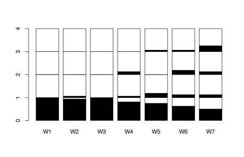
In weeks 1 and 3 every subject scores 1; from week 4 on the black share of band 1 shrinks (from 1 to 0.5 in week 7) while the higher bands fill, so the burning sensation gets steadily worse over the seven weeks.
7.4- Suppress the default axes and week names (axes = FALSE, names.arg), then add them back with axis() (Section 7.5.2): side 3 at the bar midpoints returned by barplot() for the weeks, side 2 at the band centres 0.5, 1.5, 2.5, 3.5 for the scores, both with col.axis = "blue"; the title is added with title() (Section 7.5.1), raised with line = 3 so it clears the top axis.
bp <- barplot(M, col = c("red", "white"), axes = FALSE,
names.arg = rep("", 7))
axis(3, at = bp, labels = colnames(M), col.axis = "blue", tick = FALSE)
axis(2, at = 0:3 + 0.5, labels = 1:4, col.axis = "blue", las = 1,
tick = FALSE)
title("Burning sensation: frequency of each score by week", line = 3)
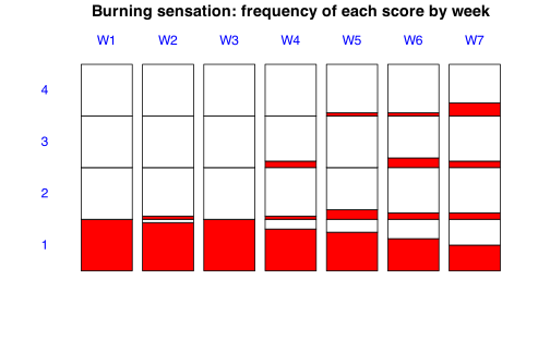
Worksheet 7.W.D — Anatomic images of the brain
Worksheet 7.W.D — Anatomic images of the brain
Data acquired during Magnetic Resonance Imaging (MRI) of the brain are usually stored as a binary file with extension *.img. We shall see how to read and display such data.
7.1- Import the file http://www.biostatisticien.eu/springeR/anat.img, which contains the image of a single brain section of \(256 \times 256\) pixels, using the function readBin(). These data can be treated as a sequence of \(256 \times 256\) byte pairs (raw). Store these data in an object called bytes.
7.2- When the data were recorded, each pair of bytes was in fact written in reverse (for example, the pair 02 56 was recorded as 56 02). You therefore need to permute each byte pair. Store the result of this operation in x.
7.3- This sequence of byte pairs now needs to be transformed into numeric values which can be displayed graphically. With two bytes (such as 02 56), you can use the instruction as.numeric("0x0256") to get the corresponding decimal value (in this case, the result is 598). Transform x into decimal values and store the result in an object called values (hint: use the functions matrix(), apply() and paste()).
7.4- Recreate the matrix of size \(256 \times 256\) containing the observations stored in values. Call this matrix X.
7.5- Use the function image() on X. Use a colour gradient of shades of grey with about one hundred shades, using the function gray().
7.6- Note that the R package AnalyzeFMRI does exactly that. After downloading the two files http://www.biostatisticien.eu/springeR/anat.img and http://www.biostatisticien.eu/springeR/anat.hdr, and after installing package AnalyzeFMRI, you could have got the exact same result by typing:
require(AnalyzeFMRI)
Y <- f.read.volume("/path/to/anat.img") # Replace path.
image(X,col=gray(0:1000 / 1000))
7.1- Open a binary connection to the URL and read its \(2 \times 256 \times 256 = 131072\) bytes as raw:
con <- url("http://www.biostatisticien.eu/springeR/anat.img", open = "rb")
bytes <- readBin(con, what = "raw", n = 2 * 256 * 256)
close(con)
length(bytes)
head(bytes)
[1] 131072
[1] 56 02 c4 02 64 02
7.2- Put the bytes in a two-row matrix (one column per pair), swap the rows and flatten back:
x <- as.vector(matrix(bytes, nrow = 2)[2:1, ])
head(x)
[1] 02 56 02 c4 02 64
7.3- For each column (byte pair) of the two-row matrix, paste() the two hexadecimal bytes behind "0x" and convert with as.numeric():
values <- as.numeric(apply(matrix(x, nrow = 2), 2,
function(b) paste0("0x", b[1], b[2])))
head(values)
range(values)
[1] 598 708 612 624 429 576
[1] 93 24088
The first pixel is 598, the value quoted in the statement; intensities run from 93 to 24088.
7.4- The pixels are stored column by column, so matrix() with its default byrow = FALSE rebuilds the image:
X <- matrix(values, nrow = 256, ncol = 256)
dim(X)
[1] 256 256
7.5- image() (Section 7.3.3) with col = gray(0:100 / 100), i.e. 101 grey levels from black to white, shows a sagittal section of the head:
par(mar = c(0, 0, 0, 0))
image(X, col = gray(0:100 / 100), axes = FALSE, asp = 1, useRaster = TRUE)
7.6- With AnalyzeFMRI (version 1.1-26 from CRAN) f.read.volume() reads the Analyze header anat.hdr and returns a \(256 \times 256 \times 1\) array whose single slice is identical to our X:
download.file("http://www.biostatisticien.eu/springeR/anat.img", "anat.img",
mode = "wb", quiet = TRUE)
download.file("http://www.biostatisticien.eu/springeR/anat.hdr", "anat.hdr",
mode = "wb", quiet = TRUE)
require(AnalyzeFMRI)
Y <- f.read.volume("anat.img")
dim(Y)
all.equal(Y[, , 1], X, check.attributes = FALSE)
[1] 256 256 1
[1] TRUE
So image(Y[, , 1], col = gray(0:1000 / 1000)) redraws the figure of 7.5; the book’s last line image(X, ...) should read image(Y[, , 1], ...) (erratum), since the object just read is Y and it is three-dimensional.
Worksheet 7.W.E — Drawing the map of a region of France
Worksheet 7.W.E — Drawing the map of a region of France
The package maps includes maps of various countries. We shall use it to draw the borders of a French département.
7.1- Install and load the packages maps and mapdata.
7.2- Draw the map of France: map("france").
7.3- Get the data on borders of French regions: france <- map("france",plot=FALSE)
7.4- Display the contents of the object france and make sure you understand how it is organized. For example, note that latitude and longitude data are stored in france$x / france$y for each département in france$names (until the next NA).
7.5- Create a vector indNA containing the indices of missing values.
7.6- Create an object containing the name of the département of your choice (for example depname <- "Gard").
7.7- Create an object called inddept containing the département index depname in the vector france$names.
7.8- Draw the map of your département.
7.9- Add a point for a place on the map. You can get the coordinates (latitude and longitude) of a place on the website http://www.gpsvisualizer.com/geocode.
7.1- install.packages() once, then library() in every session (mapdata only adds high-resolution databases such as "worldHires"; the "france" map itself ships with maps).
install.packages(c("maps", "mapdata"))
library(maps)
library(mapdata)
7.2- A single call draws the borders of the 96 metropolitan départements (Corsica included) held in the database.
map("france")
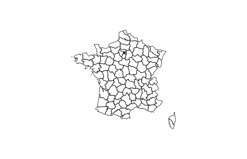
7.3- With plot = FALSE, map() returns the coordinates instead of drawing them.
france <- map("france", plot = FALSE)
7.4- france is a list of class "map" with four components: x (longitudes) and y (latitudes), both of length 13466, range (the bounding box) and names (114 polyline names).
str(france)
head(france$names, 6)
head(cbind(x = france$x, y = france$y), 3)
List of 4
$ x : num [1:13466] 2.56 2.58 2.61 2.63 2.63 ...
$ y : num [1:13466] 51.1 51 51 51 50.9 ...
$ range: num [1:4] -5.14 9.56 41.37 51.1
$ names: chr [1:114] "Nord" "Pas-de-Calais" "Somme" "Nord:1" ...
- attr(*, "class")= chr "map"
[1] "Nord" "Pas-de-Calais" "Somme" "Nord:1"
[5] "Ardennes" "Seine-Maritime"
x y
[1,] 2.557093 51.09752
[2,] 2.579995 51.00298
[3,] 2.609101 50.98545
The x=/=y vectors are the 114 polygons laid end to end and separated by NA: the \(k\)-th stretch between two NA values is the outline named france$names[k]; a département drawn in several pieces (islands, enclaves) gets extra names such as "Nord:1".
7.5- which(is.na()) gives the 113 separators (france$y has its NA values at the same positions).
indNA <- which(is.na(france$x))
length(indNA)
head(indNA)
[1] 113
[1] 206 372 533 547 696 796
7.6- A character string of length 1:
depname <- "Gard"
7.7- which() on a logical comparison; Gard is the 92nd outline and is drawn in one piece (no "Gard:1").
inddept <- which(france$names == depname)
inddept
[1] 92
7.8- Padding indNA with 0 and length(france$x) + 1 lets the \(k\)-th outline run from bounds[k] + 1 to bounds[k + 1] - 1; polygon() then fills it, and asp \(= 1/\cos(\text{latitude})\) keeps a degree of longitude to its true length (map("france", regions = depname) draws the same outline in one call).
bounds <- c(0, indNA, length(france$x) + 1)
ind <- (bounds[inddept] + 1):(bounds[inddept + 1] - 1)
x <- france$x[ind]; y <- france$y[ind]
plot(x, y, type = "n", asp = 1 / cos(mean(y) * pi / 180),
xlab = "Longitude", ylab = "Latitude", main = depname)
polygon(x, y, col = "lightyellow", border = "darkgreen", lwd = 2)
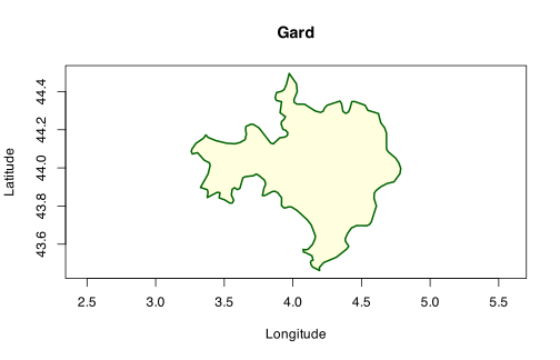
7.9- points() adds the place with longitude on the \(x\)-axis and latitude on the \(y\)-axis; here Nîmes, the préfecture of the Gard, at latitude 43.8367 N and longitude 4.3601 E (its standard geocoded position; any place looked up on the gpsvisualizer site is added the same way).
points(4.3601, 43.8367, pch = 19, col = "red")
text(4.3601, 43.8367, "Nimes", pos = 4, col = "red")
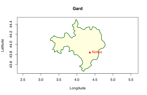
Worksheet 7.W.F — Representation of the geoid in France
Worksheet 7.W.F — Drawing curves and plots — Representation of the geoid in France
A geoid can be seen as a gravitation equipotential surface, going through the average sea level datum.
7.1- Import the file http://www.biostatisticien.eu/springeR/raf98.gra in a matrix, using the function scan(). First, read the associated file http://www.biostatisticien.eu/springeR/geoidformat.txt which gives a description of the file format.
7.2- Try to reproduce the plot available at
 . Do not try to superpose the map of France yet (hint: use the functions
 scan(), layout(), par(), image(), axis(), contour(), legend() and rainbow()).
7.1- Read everything with scan(), drop the six header values and fill a \(381 \times 421\) matrix byrow = TRUE. The format file says the header holds the south/north latitude limits (42, 51.5), the west/east longitude limits (-5.5, 8.5) and the steps (0.025 and 1/30 degree), and that the grid is stored latitude by latitude from north to south, each latitude running west to east.
x <- scan("http://www.biostatisticien.eu/springeR/raf98.gra", quiet = TRUE)
length(x)
hdr <- x[1:6]; hdr
geoid <- matrix(x[-(1:6)], nrow = 381, ncol = 421, byrow = TRUE)
dim(geoid)
range(geoid)
geoid[1:3, 1:4]
[1] 160407
[1] 42.00000000 51.50000000 -5.50000000 8.50000000 0.02500000 0.03333333
[1] 381 421
[1] 41.8493 55.4308
[,1] [,2] [,3] [,4]
[1,] 53.3573 53.3569 53.3546 53.3481
[2,] 53.3284 53.3277 53.3259 53.3209
[3,] 53.3056 53.3023 53.2990 53.2940
Since \(160407 = 6 + 381 \times 421\), row 1 of geoid is the northern edge (\(51.5^\circ\)N) and column 1 the western edge (\(5.5^\circ\)W); geoid heights above the ellipsoid run from 41.8 m to 55.4 m.
7.2- The page geoid.png now returns HTTP 404, so the target could not be compared directly. The code below makes the plot the hints describe: a filled image() in rainbow() colours with contour() lines at 1 m intervals, custom axis() calls, and a legend() in a second panel created with layout(). image() expects rows indexed by \(x\) (longitude, increasing) and columns by \(y\) (latitude, increasing), so the matrix is flipped north to south and then transposed.
lon <- seq(-5.5, 8.5, length.out = 421)
lat <- seq(42, 51.5, length.out = 381)
z <- t(geoid[381:1, ]) # rows = longitudes W->E, cols = latitudes S->N
brk <- seq(41, 56, by = 1)
cols <- rev(rainbow(length(brk) - 1, end = 0.7))
layout(matrix(1:2, nrow = 1), widths = c(4, 1))
par(mar = c(4, 4, 3, 1))
image(lon, lat, z, breaks = brk, col = cols, axes = FALSE, useRaster = TRUE,
xlab = "Longitude (degrees)", ylab = "Latitude (degrees)",
main = "RAF98 geoid height above the ellipsoid (m)")
axis(1, at = seq(-5, 8, by = 1)); axis(2, at = seq(42, 51, by = 1), las = 1)
box()
contour(lon, lat, z, levels = brk, add = TRUE, labcex = 0.6)
par(mar = c(4, 0, 3, 0))
plot.new()
legend("center", legend = rev(paste(brk[-length(brk)], "-", brk[-1])),
fill = rev(cols), title = "Height (m)", bty = "n", cex = 0.8)
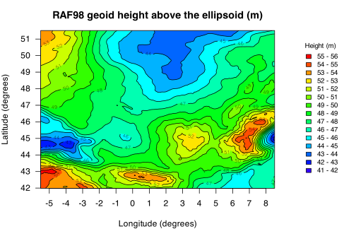
The geoid is highest over the northern Spanish coast in the southwest corner (maximum 55.4 m near \(4.8^\circ\)W, \(43^\circ\)N), the Alps (about 54.6 m near \(7^\circ\)E, \(45.5^\circ\)N) and the Pyrenees (about 54 m). It is lowest, below 45 m, over the Paris Basin and Channel, in the Bay of Biscay near \(4.5^\circ\)W, \(44.5^\circ\)N, and off the Ligurian coast (minimum 41.8 m at \(8.5^\circ\)E, \(45^\circ\)N).
Programming in R
Exercises 8.1–8.7
For each of the following command lines, indicate the class of the returned R object. What is displayed upon execution of each of these command lines?
function(name) {name}(function(name) {name})("Ben")(function(name) {cat(name,"\n")})("Ben")(function(name) {invisible(name)})("Ben")
The classes are "function", "character", "NULL" and "character"; only the first two lines auto-print their value, the third displays Ben as a side effect of cat() (its value is the invisible NULL of cat()) and the fourth displays nothing, since invisible() suppresses auto-printing of "Ben".
function(name) {name}
(function(name) {name})("Ben")
(function(name) {cat(name,"\n")})("Ben")
(function(name) {invisible(name)})("Ben")
sapply(list(function(name) {name},
(function(name) {name})("Ben"),
(function(name) {cat(name,"\n")})("Ben"),
(function(name) {invisible(name)})("Ben")), class)
function(name) {name}
[1] "Ben"
Ben
Ben
[1] "function" "character" "NULL" "character"
Is there a difference between
name <- function(name) nameandname <- function(name) {name}name <- function(name) {name}andname <- function(name) {return(name)}name <- function(name) {name}and(function(name) {name}) -> name
No difference in behaviour: all four declarations define a function returning its argument (Section 8.2). The braces only turn the body into a call to "{"() instead of the bare symbol, return() is redundant when it wraps the last instruction, and -> is the right-to-left assignment of the same function object.
f1 <- function(name) name ; f2 <- function(name) {name}
f3 <- function(name) {return(name)}
(function(name) {name}) -> f4
c(f1("Ben"), f2("Ben"), f3("Ben"), f4("Ben"))
identical(f2, f4, ignore.srcref = TRUE)
[1] "Ben" "Ben" "Ben" "Ben"
[1] TRUE
Upon execution, is there a difference between name() and name("Peter") when
name <- function(name“Peter”) name=name <- function(name“Peter”) name2 <- name=
For these two declarations of the function name(), is there a difference in the type of the R object res given by res <- name("Ben")?
No: in both declarations name() and name("Peter") are the same call, because "Peter" is the default value. The first version prints [1] "Peter"; the second prints nothing, since its last instruction is an assignment, whose value is returned invisibly.
name <- function(name="Peter") name
name(); name("Peter")
name <- function(name="Peter") name2 <- name
name(); name("Peter")
res <- name("Ben"); class(res); (name("Ben"))
[1] "Peter"
[1] "Peter"
[1] "character"
[1] "Ben"
The type of res is the same: in both cases res is the character string "Ben", because the value of the assignment name2 <- name is its right-hand side.
What R object is returned upon execution of name() when:
name <- function(name="Peter") {
name
# The last instruction is a comment!
}
The character string "Peter": a comment is not an instruction, so name is still the last evaluated expression of the block.
name <- function(name="Peter") {
name
# The last instruction is a comment!
}
name()
[1] "Peter"
When name <- function(firstname“Peter”,name=“L”) {paste(firstname,name)}=, what R object is returned by
name(firstname“Ben”)=name(fir“Ben”)=name(n“D”,f=“R”)=
The strings "Ben L", "Ben L" and "R D": arguments are matched by partial name (fir, f to firstname; n to name), and the missing one takes its default.
name <- function(firstname="Peter",name="L") {
paste(firstname,name)}
name(firstname="Ben")
name(fir="Ben")
name(n="D",f="R")
[1] "Ben L"
[1] "Ben L"
[1] "R D"
Rewrite the following function declaration in one line, without using the command separator “;”:
name <- function(name) { if(missing("name"))
name <- "Peter"; cat(name,"\n") }
Give the argument a default value: name <- function(name = "Peter") cat(name, "\n"); keeping missing() is also possible with name <- function(name) cat(if (missing(name)) "Peter" else name, "\n").
name <- function(name = "Peter") cat(name, "\n")
name(); name("Ben")
Peter
Ben
What is the output of the execution of names("peteR","Ben","R") when:
names <- function(...) c(...)names <- function(...) list(...)names <- function(...) for(name in c(...)) print(name)names <- function(...) for(name in list(...)) print(name)
Same question upon execution of names(c("peteR","L"),c("Ben","L"),c("R","D")).
With c(...) the arguments are concatenated into one character vector, with list(...) each argument stays a separate list element, and the for versions print element by element (then return NULL invisibly).
names <- function(...) c(...)
names("peteR","Ben","R")
names(c("peteR","L"),c("Ben","L"),c("R","D"))
names <- function(...) list(...)
names("peteR","Ben","R")
[1] "peteR" "Ben" "R"
[1] "peteR" "L" "Ben" "L" "R" "D"
[[1]]
[1] "peteR"
[[2]]
[1] "Ben"
[[3]]
[1] "R"
With the three pairs, list(...) gives a list of three vectors of length 2:
names(c("peteR","L"),c("Ben","L"),c("R","D"))
[[1]]
[1] "peteR" "L"
[[2]]
[1] "Ben" "L"
[[3]]
[1] "R" "D"
For the loops, iterating over c(...) visits the six single strings, while iterating over list(...) visits the three vectors; with single strings as arguments both loops print the same three lines.
names <- function(...) for(name in c(...)) print(name)
names("peteR","Ben","R")
names(c("peteR","L"),c("Ben","L"),c("R","D"))
names <- function(...) for(name in list(...)) print(name)
names("peteR","Ben","R")
names(c("peteR","L"),c("Ben","L"),c("R","D"))
[1] "peteR"
[1] "Ben"
[1] "R"
[1] "peteR"
[1] "L"
[1] "Ben"
[1] "L"
[1] "R"
[1] "D"
[1] "peteR"
[1] "Ben"
[1] "R"
[1] "peteR" "L"
[1] "Ben" "L"
[1] "R" "D"
Exercises 8.8–8.11
When names <- function(names=c("Ben","R"),...) c(names,...), which R objects are returned by names("PeteR"), names(name“PeteR”)= and names(names“PeteR”)=? Same question when names <- function(...,names=c("Ben","R")) c(names,...).
With names placed before ..., all three calls return "PeteR": the first by position, the second by partial matching of name to names, the third by exact name. With names placed after ..., it can only be matched by its exact name, so the first two calls put "PeteR" into ... (keeping the tag name in the second) and the default c("Ben","R") is kept.
names <- function(names=c("Ben","R"),...) c(names,...)
names("PeteR"); names(name="PeteR"); names(names="PeteR")
names <- function(...,names=c("Ben","R")) c(names,...)
names("PeteR"); names(name="PeteR"); names(names="PeteR")
rm(names) # restore base::names()
[1] "PeteR"
[1] "PeteR"
[1] "PeteR"
[1] "Ben" "R" "PeteR"
name
"Ben" "R" "PeteR"
[1] "PeteR"
Create a constructor function Male() generating an object of class "Male" with fields firstname and name (in an object of type list). Create the method hello.Male() which displays "Hello Mister FIRSTNAME NAME!" (do not forget the "\n" at the end of the display!) for an object with values "FIRSTNAME" and "NAME" respectively for the fields firstname and name. When man <- Male("Ben","L"), what is produced upon execution of the following commands: hello.Male(man) and hello(man)? What code should you execute in addition for the two results to be identical?
hello.Male(man) displays Hello Mister Ben L! but hello(man) fails because the generic hello() does not exist; declaring it with hello <- function(obj, ...) UseMethod("hello") (Section 8.3) makes both calls identical.
Male <- function(firstname, name) {
obj <- list(firstname = firstname, name = name)
class(obj) <- "Male"
obj
}
hello.Male <- function(obj) cat("Hello Mister", obj$firstname, paste0(obj$name, "!"), "\n")
man <- Male("Ben", "L")
hello.Male(man)
hello(man)
Hello Mister Ben L!
Error in hello(man) : could not find function "hello"
hello <- function(obj, ...) UseMethod("hello")
hello(man)
Hello Mister Ben L!
Create the analogous functions for the class "Female" (hint: do not forget to update the gender in hello.Female()). When woman <- Female("Elsa","R"), what is produced upon execution of the following commands: hello.Male(woman), hello.Female(woman) and hello(woman).
hello.Male(woman) displays Hello Mister Elsa R! (a method called directly does not check the class), whereas hello.Female(woman) and hello(woman) both display Hello Madam Elsa R!, the generic dispatching on the class "Female".
Female <- function(firstname, name) {
obj <- list(firstname = firstname, name = name)
class(obj) <- "Female"
obj
}
hello.Female <- function(obj) cat("Hello Madam", obj$firstname, paste0(obj$name, "!"), "\n")
woman <- Female("Elsa", "R")
hello.Male(woman)
hello.Female(woman)
hello(woman)
Hello Mister Elsa R!
Hello Madam Elsa R!
Hello Madam Elsa R!
When welcome <- function(...) for(person in list(...)){hello(person)}, what is returned by welcome(man,woman)? And when welcome <- function(...) for(person in c(...)){hello(person)}? Same question when hello.default <- function(obj){cat("hello",obj,"!\n")}.
With list(...) each person keeps its class, so the two greetings Hello Mister Ben L! and Hello Madam Elsa R! are displayed (the loop itself returns NULL invisibly). With c(...) the two objects are merged into a plain list of four character strings (the class attribute is dropped), so hello() is called on "Ben" and stops with an error.
welcome <- function(...) for(person in list(...)){
hello(person)}
welcome(man,woman)
welcome <- function(...) for(person in c(...)){
hello(person)}
welcome(man,woman)
Hello Mister Ben L!
Hello Madam Elsa R!
Error in UseMethod("hello") :
no applicable method for 'hello' applied to an object of class "character"
Once hello.default() is defined, the c(...) version no longer fails: each of the four strings goes to the default method, while the list(...) version is unchanged.
hello.default <- function(obj){
cat("hello",obj,"!\n")}
welcome(man,woman)
welcome <- function(...) for(person in list(...)){
hello(person)}
welcome(man,woman)
hello Ben !
hello L !
hello Elsa !
hello R !
Hello Mister Ben L!
Hello Madam Elsa R!
Worksheet 8.W.B — Organizing graphical objects
Worksheet 8.W.B — Organizing graphical objects — Organizing graphical objects
When you think about it, plots in R do not really respect the object-oriented spirit: unlike most other entities, an R plot is not considered as an object which can be saved (and possibly modified) and on which certain methods can be applied. We shall attempt to propose a very basic prototype to draw a plot with circles and rectangles (and hence squares). You can enrich this library with graphical objects as you wish. Our aim is to maintain a list of graphical objects, with the possibility of changing any of its elements at any time.
8.1- R functions plot.new() and plot.window() are used to initialize a plot. The argument asp set to 1 creates plots with correct units for the \(x\) and \(y\) axes. Propose an object Window which gives the user the option of saving the dimensions of the graphics display window. The user can then call the constructor function (or method) Window() (which could have the same name as the class), which takes as arguments x and y (the coordinates of the centre), width, height (dimensions along the \(x\) and \(y\) axes respectively) and optionally log (logarithmic transformation). All these quantities should be stored in an object list, returned by the constructor function Window(), after affecting its class to "Window".
8.2- Similarly, propose constructor functions for objects of classes Circle and Rectangle. The fields x and y represent the coordinates of the centre of the object, radius is the radius of a circle and width and height are the dimensions of a rectangle.
8.3- Propose plotting methods plot.Window(), plot.Rectangle() and plot.Circle(). You can find inspiration in the following R treatments used to display a new plot with a circle and a square centred at the origin and of diameter and side length set to 1:
plot.new()
plot.window(xlim=c(-1,1),ylim=c(-1,1),asp=1)
rect(-.5,-.5,.5,.5)
symbols(0,0,circle=.5,inches=FALSE,add=TRUE)
8.4- Test the code you have developed by executing the code:
mywindow <- Window(0,0,2,2)
mycircle <- Circle(0,0,.5)
myrectangle <- Rectangle(0,0,1,1)
plot(mywindow);plot(mycircle);plot(myrectangle)
If all goes well, you should see a graphics window with a circle inside a square.
8.5- We now need to develop the methods associated with the class MyPlot which will contain the list of all graphical objects. First, propose a constructor function MyPlot() which initializes an object as list(objects=list()) (where objects is the field containing the list of graphical objects), affects the class "MyPlot" and returns the object.
8.6- Propose a method add.MyPlot() which adds graphical objects. Remember to give a generic function add() to launch all associated methods. Use the functionalities of the list of supplementary arguments ... and the function c() so that the method add.MyPlot() can initialize as many graphical objects as the user wishes. Propose a method plot.MyPlot() which executes the methods plot() for all graphical objects. The user can then enter the following lines to get the same result as earlier:
myplot <- MyPlot()
myplot <- add(myplot,Window(0,0,2,2),Circle(0,0,.5),
Rectangle(0,0,1,1))
plot(myplot)
8.7- To display a plot, you need to initialize an object of type Window and put it in first position of the list of graphical objects of the class MyPlot. It might be useful to initialize it directly inside the constructor function MyPlot(). The arguments of the function Window() can be proposed directly for the function MyPlot(). Another idea is to propose a list of graphical objects to the user upon creation of an object of class MyPlot. As we have done for the method add.MyPlot(), we could use the list of supplementary arguments ..., which must be placed as first argument of the function MyPlot() so as to get the previous result with only two lines:
myplot <- MyPlot(Circle(),Rectangle())
plot(myplot)
However, note that in the first line, it is assumed that the default values of the arguments of the function Window(), Circle() and Rectangle() are appropriate.
8.8- The project is launched with this first prototype. You can complete it as you wish. If you need inspiration, you could try managing the list of graphical objects (for example, deleting or modifying an object), display styles, axes…
8.1- Window() stores its five arguments in a list and sets the class attribute (S3 constructor, Section 8.3); the defaults (a \(2\times 2\) window centred at the origin) are chosen with question 8.7 in mind.
Window <- function(x = 0, y = 0, width = 2, height = 2, log = "") {
obj <- list(x = x, y = y, width = width, height = height, log = log)
class(obj) <- "Window"
obj
}
str(Window(0, 0, 2, 2))
List of 5
$ x : num 0
$ y : num 0
$ width : num 2
$ height: num 2
$ log : chr ""
- attr(*, "class")= chr "Window"
8.2- The two constructors follow the same pattern, with defaults giving the unit-diameter circle and the unit square of question 8.3.
Circle <- function(x = 0, y = 0, radius = 0.5) {
obj <- list(x = x, y = y, radius = radius)
class(obj) <- "Circle"
obj
}
Rectangle <- function(x = 0, y = 0, width = 1, height = 1) {
obj <- list(x = x, y = y, width = width, height = height)
class(obj) <- "Rectangle"
obj
}
class(Circle(0, 0, .5)); unlist(Rectangle(0, 0, 1, 1))
[1] "Circle"
x y width height
0 0 1 1
8.3- Each method converts the centre/size fields into the arguments of plot.window(), rect() and symbols(); since plot() is already generic, defining plot.<class>() is enough for dispatch. (The book’s circle.5= works only through partial matching of the argument circles.)
plot.Window <- function(x, ...) {
plot.new()
plot.window(xlim = x$x + c(-1, 1) * x$width / 2,
ylim = x$y + c(-1, 1) * x$height / 2, asp = 1, log = x$log)
invisible(x)
}
plot.Rectangle <- function(x, ...) {
rect(x$x - x$width / 2, x$y - x$height / 2,
x$x + x$width / 2, x$y + x$height / 2, ...)
invisible(x)
}
plot.Circle <- function(x, ...) {
symbols(x$x, x$y, circles = x$radius, inches = FALSE, add = TRUE, ...)
invisible(x)
}
8.4- The test code draws the expected circle inscribed in the unit square.
mywindow <- Window(0,0,2,2)
mycircle <- Circle(0,0,.5)
myrectangle <- Rectangle(0,0,1,1)
plot(mywindow);plot(mycircle);plot(myrectangle)
8.5- The first constructor simply wraps an empty list in the class "MyPlot".
MyPlot <- function() {
obj <- list(objects = list())
class(obj) <- "MyPlot"
obj
}
str(MyPlot())
List of 1
$ objects: list()
- attr(*, "class")= chr "MyPlot"
8.6- The generic add() dispatches with UseMethod(); add.MyPlot() appends list(...) to the field objects with c(), and plot.MyPlot() calls plot() on each element, which dispatches to the methods of 8.3. The book’s three lines give the same figure as in 8.4.
add <- function(obj, ...) UseMethod("add")
add.MyPlot <- function(obj, ...) {
obj$objects <- c(obj$objects, list(...))
obj
}
plot.MyPlot <- function(x, ...) {
for (o in x$objects) plot(o)
invisible(x)
}
myplot <- MyPlot()
myplot <- add(myplot,Window(0,0,2,2),Circle(0,0,.5),
Rectangle(0,0,1,1))
sapply(myplot$objects, class)
plot(myplot)
[1] "Window" "Circle" "Rectangle"
8.7- MyPlot() now takes ... first, then the arguments of Window() (which must be named when called, since they follow ...), puts the window in position 1 and hands the other objects to add(); the two-line call reproduces the figure.
MyPlot <- function(..., x = 0, y = 0, width = 2, height = 2, log = "") {
obj <- list(objects = list(Window(x, y, width, height, log)))
class(obj) <- "MyPlot"
add(obj, ...)
}
myplot <- MyPlot(Circle(),Rectangle())
sapply(myplot$objects, class)
plot(myplot)
[1] "Window" "Circle" "Rectangle"
8.8- One possible extension: a style field whose entries are passed to rect()=/=symbols() through do.call(), an axes field for the window, and the new generics delete() and modify() for managing the list (the window in position 1 is protected); in the figure the unit circle has been deleted, the square styled, the small circle moved and an orange rectangle added on a wider window with axes.
style <- function(obj, ...) {
obj$style <- modifyList(as.list(obj$style), list(...)); obj
}
plot.Rectangle <- function(x, ...)
do.call(rect, c(list(x$x - x$width/2, x$y - x$height/2,
x$x + x$width/2, x$y + x$height/2), x$style))
plot.Circle <- function(x, ...)
do.call(symbols, c(list(x$x, x$y, circles = x$radius,
inches = FALSE, add = TRUE), x$style))
plot.Window <- function(x, ...) {
plot.new()
plot.window(xlim = x$x + c(-1, 1) * x$width / 2,
ylim = x$y + c(-1, 1) * x$height / 2, asp = 1, log = x$log)
if (isTRUE(x$axes)) { axis(1); axis(2); box() }
invisible(x)
}
delete <- function(obj, ...) UseMethod("delete")
delete.MyPlot <- function(obj, i) {
if (any(i == 1)) stop("the Window (object 1) cannot be deleted")
obj$objects <- obj$objects[-i]; obj
}
modify <- function(obj, ...) UseMethod("modify")
modify.MyPlot <- function(obj, i, ...) {
obj$objects[[i]] <- modifyList(obj$objects[[i]], list(...)); obj
}
myplot <- MyPlot(Circle(), Rectangle(), Circle(.5, .5, .25), width = 3)
myplot <- modify(myplot, 1, axes = TRUE)
myplot <- modify(myplot, 3, style = list(col = "lightblue", border = "navy", lwd = 2))
myplot <- modify(myplot, 4, x = -0.5)
myplot <- add(myplot, style(Rectangle(0.75, -0.5, 0.5, 0.25), col = "orange"))
myplot <- delete(myplot, 2)
sapply(myplot$objects, class)
plot(myplot)
[1] "Window" "Rectangle" "Circle" "Rectangle"
Managing sessions
Exercises 9.1–9.7
Name two R functions which return a list of objects in your session.
ls() and its synonym objects() (Section 9.1):
My.Weight <- 75; My.Height <- 1.90; foo <- 1:3
ls()
objects()
[1] "foo" "My.Height" "My.Weight"
[1] "foo" "My.Height" "My.Weight"
How would you delete the object foo?
With rm(foo) (Section 9.1); rm(list = ls()) would delete every object in the workspace.
rm(foo)
ls()
[1] "My.Height" "My.Weight"
Which R command gives the current directory?
getwd() returns the current working directory (Section 9.2); here R was started in /tmp:
getwd()
[1] "/private/tmp"
Which R command changes the current directory?
setwd("path/to/folder") (Section 9.2); here it moves into a folder Cars, as in the book’s example:
dir.create("Cars", showWarnings = FALSE)
setwd("Cars")
basename(getwd())
[1] "Cars"
What is the purpose of the function save.image()?
save.image() saves all the objects of the current workspace to a .RData file (by default .RData in the working directory), which load() restores in a later session (Section 9.2):
x <- c("FIAT", "VOLVO", "RENAULT", "PEUGEOT")
save.image("cars.RData")
rm(list = ls())
ls()
load("cars.RData")
x
character(0)
[1] "FIAT" "VOLVO" "RENAULT" "PEUGEOT"
What are the four things you can save before closing an R session?
The four things are:
- the objects of the workspace, in a
.RDatafile (save.image(), Section 9.2); - the command history, in a
.Rhistoryfile (savehistory(), Section 9.3); - the plots (
dev.print(), orpng(),pdf(), … followed bydev.off(), Section 9.4); - the text output of the console (
sink(file = "myoutput.txt"), or the menu File/Save to file… under Windows, Section 9.7).
What is the purpose of the command history? Which keys are necessary to use it?
It lets you recall, edit and re-execute the commands typed earlier (and, saved with savehistory() in a .Rhistory file, reuse them in a later session); the up and down arrow keys move backward and forward through it, and the left and right arrow keys edit the recalled line before pressing Enter (Section 9.3).
Exercises 9.8–9.12
What is the purpose of the function history()?
history() opens a window listing the commands typed in the current session (by default the last 25; history(max.show = Inf) shows them all, and history(pattern = "plot") only the matching ones), Section 9.3. It only works in an interactive session, so it is not run here.
Give the list of R instructions you would use to get a file called myplot.png containing a plot of the curve \(y = x^2\).
Open a png() device on the file, draw the curve, then close the device with dev.off() so that the file is written (Section 9.4):
png("myplot.png", width = 480, height = 480)
curve(x^2, from = -3, to = 3)
dev.off()
file.exists("myplot.png")
null device
1
[1] TRUE
Equivalently, draw curve(x^2, from = -3, to = 3) on screen and copy it with dev.print(png, file = "myplot.png", width = 480, height = 480). The plot stored in the file:
curve(x^2, from = -3, to = 3)
When is the function attach() useful for a data.frame?
When you work repeatedly with the variables of one data frame: attach(mydata) puts it in position 2 of the search path, so its columns can be called directly by name instead of mydata$breaks (Section 9.6); undo it with detach(mydata).
mydata <- warpbreaks
attach(mydata)
search()[1:3]
tapply(breaks, tension, mean)
detach(mydata)
[1] ".GlobalEnv" "mydata" "package:stats"
L M H
36.38889 26.38889 21.66667
Which R function is used to load an R package to the memory?
require() (or library()), for a package already installed on the disk; require() does nothing if the package is already loaded (Section 9.5):
require(MASS)
"package:MASS" %in% search()
Loading required package: MASS
[1] TRUE
What is the purpose of the function source()?
source("myfile.R") reads a file of R instructions and executes them all in the console, after checking their syntax (Section 9.7); source(file.choose()) lets you pick the file interactively.
writeLines(c("sq <- function(x) x^2", "z <- sq(1:5)"), "myfile.R")
source("myfile.R")
z
[1] 1 4 9 16 25
Worksheet 9.W.A — Using the functions attach() and detach()
Worksheet 9.W.A — Managing and creating packages — Using the functions attach() and detach()
9.1- Download the file http://www.biostatisticien.eu/springeR/bmichild.xls.
9.2- Display the names of the variables of the data.frame.
9.3- Type GENDER. What do you observe?
9.4- Type ls(). Can you see the variable GENDER?
9.5- Use the function attach() on your data.frame, then type GENDER. What do you observe now?
9.6- Type ls() again. What do you observe?
9.7- Use the function search() to find the position at which your data.frame is attached.
9.8- Use the argument pos of the function ls() to list the objects present at this position.
9.9- Detach your data.frame and check (using the function search()) that it worked. Now type GENDER again and observe that this object has disappeared.
9.10- Create an object called GENDER containing the string "Male". Display the contents of this object.
9.11- Use the function attach() on your data.frame then type GENDER. What do you observe?
9.12- Can you display the contents of the object GENDER of your data.frame? How about the object weight?
9.13- Type ls(). What do you observe? How about with search()?
9.14- Use the argument pos of the function ls() to check that the object GENDER of the data.frame does exist.
9.15- Use the function get() and its argument pos to display the contents of the object GENDER from your data.frame. Can you propose another approach?
9.1- Download the file and read it into a data.frame bmi. The book used read.xls() from gdata, which newer gdata versions no longer provide, so this uses readxl::read_excel(). The :: call avoids attaching readxl, which would shift the positions in search() below.
download.file("http://www.biostatisticien.eu/springeR/bmichild.xls",
"bmichild.xls", mode = "wb", quiet = TRUE)
bmi <- as.data.frame(readxl::read_excel("bmichild.xls"))
9.2- names(bmi) lists the variables: gender, ZEP status, weight, age in years and months, and height.
names(bmi)
[1] "GENDER" "zep" "weight" "year" "month" "height"
9.3- R cannot find GENDER. It exists only as a column inside bmi, and R does not look inside a data.frame when it resolves a name.
try(GENDER)
Error : object 'GENDER' not found
9.4- No. The workspace contains only the data.frame itself.
ls()
[1] "bmi"
9.5- GENDER now prints the 152 genders. attach() has put the columns of bmi on the search path (Section 9.6). Only the first 10 values are shown here.
attach(bmi)
head(GENDER, 10)
[1] "F" "F" "M" "F" "M" "M" "M" "M" "M" "M"
9.6- ls() still shows only bmi. ls() lists only the global environment. The attached columns are a copy that sits in a separate database further down the search path.
ls()
[1] "bmi"
9.7- The data.frame is attached at position 2, just after .GlobalEnv.
search()
match("bmi", search())
[1] ".GlobalEnv" "bmi" "package:stats"
[4] "package:graphics" "package:grDevices" "package:utils"
[7] "package:datasets" "package:methods" "Autoloads"
[10] "package:base"
[1] 2
9.8- ls(pos = 2) lists the six variables of the data.frame, in alphabetical order.
ls(pos = 2)
[1] "GENDER" "height" "month" "weight" "year" "zep"
9.9- After detach(), "bmi" is gone from search() and GENDER is again not found.
detach(bmi)
search()
try(GENDER)
[1] ".GlobalEnv" "package:stats" "package:graphics"
[4] "package:grDevices" "package:utils" "package:datasets"
[7] "package:methods" "Autoloads" "package:base"
Error : object 'GENDER' not found
9.10- Assign the string, then print it.
GENDER <- "Male"
GENDER
[1] "Male"
9.11- R warns that the column GENDER of bmi is masked by the global object, and typing GENDER returns "Male". R searches .GlobalEnv (position 1) before the attached data.frame (position 2).
attach(bmi)
GENDER
The following object is masked _by_ .GlobalEnv:
GENDER
[1] "Male"
9.12- Typing GENDER cannot display the data.frame’s column, because the global "Male" is always found first. weight has no global homonym, so it is found in the attached bmi and displays normally.
head(weight)
[1] 16.0 14.0 13.5 15.4 16.5 16.0
9.13- ls() now shows bmi and the global GENDER. search() shows bmi attached again at position 2. The data.frame’s GENDER does not appear in ls(), which only lists position 1.
ls()
search()
[1] "bmi" "GENDER"
[1] ".GlobalEnv" "bmi" "package:stats"
[4] "package:graphics" "package:grDevices" "package:utils"
[7] "package:datasets" "package:methods" "Autoloads"
[10] "package:base"
9.14- ls(pos = 2) confirms that the masked GENDER is still present in the attached data.frame.
ls(pos = 2)
[1] "GENDER" "height" "month" "weight" "year" "zep"
9.15- get("GENDER", pos = 2) reads GENDER directly from position 2, which bypasses the global object. A simpler alternative is to take the column from the data.frame itself with bmi$GENDER. bmi[["GENDER"]] and with(bmi, GENDER) also work, and none of the three needs attach().
head(get("GENDER", pos = 2), 10)
head(bmi$GENDER, 10)
[1] "F" "F" "M" "F" "M" "M" "M" "M" "M" "M"
[1] "F" "F" "M" "F" "M" "M" "M" "M" "M" "M"
Worksheet 9.W.B.1 — Creating a mini-package - Objects in the package
Worksheet 9.W.B.1 — Creating a mini-package — Objects in the package
9.1- Start R, then change the current directory to the Windows desktop, using the instruction setwd(choose.dir()).
9.2- Create the following functions and datasets:
f <- function(x,y) x+y
g <- function(x,y) x-y
d <- data.frame(a=1,b=2)
e <- rnorm(1000)
9.1- setwd(choose.dir()) opens a folder chooser and makes the chosen folder (the desktop) the working directory; choose.dir() exists only under Windows, so on macOS or Linux type the path (or use tcltk::tk_choose.dir()):
setwd("~/Desktop") # Windows: setwd(choose.dir())
basename(getwd())
[1] "Desktop"
9.2- The four objects now live in the workspace, ready to be passed to package.skeleton() (seed 1 fixed so that e is reproducible):
f <- function(x,y) x+y
g <- function(x,y) x-y
d <- data.frame(a=1,b=2)
set.seed(1)
e <- rnorm(1000)
ls()
sapply(list(f = f, g = g, d = d, e = e), class)
[1] "d" "e" "f" "g"
f g d e
"function" "function" "data.frame" "numeric"
Worksheet 9.W.B.2 — Creating a mini-package - Package structure
Worksheet 9.W.B.2 — Creating a mini-package — Package structure
9.3- Use the function package.skeleton() to create the structure of your package.
package.skeleton(name="SmallRPkg",list=c("f","g","d","e"))
A folder called SmallRPkg is created on your desktop. It contains three sub-folders (data, man and R) and two files (DESCRIPTION and Read-and-delete-me). The folder data contains the files d.RData and e.RData, which contain respectively the datasets (in binary form) d and e, which you imported from the R console. The folder R contains the files f.R and g.R, which contain the source code of the functions f and g defined earlier. The folder man contains help files for all objects included in the package.
9.4- You must edit the help files (.Rd extension files), even if they are not empty. Use the description of the help file for the function mean in Chapter 6. The fields to fill in are made apparent in all help files by lines starting with %%. Replace those lines (including the characters %%) with the appropriate information. Do not change the sentences starting with a single %. Furthermore, in fields of the form keyword ~ kwd1, you must replace ~ kwd1 with a reserved keyword; the list of reserved keywords is given by the instruction file.show(file.path(R.home("doc"), "KEYWORDS")).
9.5- You should also change the file DESCRIPTION and fill in the relevant fields. For example, it is very important that you give a valid e-mail address.
9.6- You can then read and delete the file Read-and-delete-me.
Your package structure has now been created.
9.3- One call builds the whole tree (Section 9.10); current R additionally writes a NAMESPACE file and a package-level help page, and saves the data as d.rda and e.rda rather than the .RData files the book describes:
package.skeleton(name = "SmallRPkg", list = c("f", "g", "d", "e"))
list.files("SmallRPkg", recursive = TRUE)
Creating directories ...
Creating DESCRIPTION ...
Creating NAMESPACE ...
Creating Read-and-delete-me ...
Saving functions and data ...
Making help files ...
Done.
Further steps are described in './SmallRPkg/Read-and-delete-me'.
[1] "data/d.rda" "data/e.rda"
[3] "DESCRIPTION" "man/d.Rd"
[5] "man/e.Rd" "man/f.Rd"
[7] "man/g.Rd" "man/SmallRPkg-package.Rd"
[9] "NAMESPACE" "R/f.R"
[11] "R/g.R" "Read-and-delete-me"
9.4- Each %% placeholder is replaced by real text, the unused sections are removed, and the keyword is taken from the reserved list (arith for f and g, datasets for d and e):
kw <- readLines(file.path(R.home("doc"), "KEYWORDS"))
grep("arith|datasets", kw, value = TRUE)
[1] "\tdatasets\t&\tDatasets available by data(.)\t[!= S]"
[2] "\tarith\t\t&\tBasic Arithmetic and Sorting\t[!= S]"
The completed man/f.Rd (g.Rd is identical with “Difference”, x - y and g(5, 3); d.Rd and e.Rd keep their \format block and get a title, a \description and a \source):
\name{f}
\alias{f}
\title{Sum of Two Numbers}
\description{
Returns the sum of its two arguments.
}
\usage{
f(x, y)
}
\arguments{
\item{x}{a numeric vector.}
\item{y}{a numeric vector.}
}
\value{The numeric vector \code{x + y}.}
\author{John Doe}
\seealso{\code{\link{g}}}
\examples{
f(2, 3)
}
\keyword{arith}
In SmallRPkg-package.Rd the %% placeholder sections are simply deleted. tools::checkRd() reports no problem for any of the five files.
9.5- The completed DESCRIPTION (the Depends line is required because the data files use serialization format 3, and LazyData lets users type e without calling data(e)):
Package: SmallRPkg
Type: Package
Title: A Small Example Package
Version: 1.0
Date: 2026-09-24
Author: John Doe
Maintainer: John Doe <john.doe@example.org>
Description: Two arithmetic functions and two toy data sets, built as
the worksheet of Chapter 9 of 'The R Software'.
License: GPL-2
Depends: R (>= 3.5.0)
LazyData: true
Replace the example address with your own working address. Read-and-delete-me also says to edit NAMESPACE; set it to export("f", "g") because d and e are data sets that users get through data(), not objects in the namespace.
9.6- The file lists the remaining steps; after reading it, delete it:
cat(readLines("SmallRPkg/Read-and-delete-me"), sep = "\n")
file.remove("SmallRPkg/Read-and-delete-me")
* Edit the help file skeletons in 'man', possibly combining help files
for multiple functions.
* Edit the package 'DESCRIPTION'.
* Edit the exports in 'NAMESPACE', and add necessary imports.
* Put any C/C++/Fortran code in 'src'.
* If you have compiled code, add a useDynLib() directive to
'NAMESPACE'.
* Run R CMD build to build the package tarball.
* Run R CMD check to check the package tarball.
Read "Writing R Extensions" for more information.
[1] TRUE
Worksheet 9.W.B.3 — Creating a mini-package - Creating the package file
Worksheet 9.W.B.3 — Creating a mini-package — Creating the package file
9.7- You have one final operation to perform: building the .zip file which will include your structure (modified by R). You first need to change a few system environment variables. Use the key combination WINDOWS+PAUSE to open the system properties window, go to the section System Variables and edit the variable PATH. At the beginning of this long list of semi-colon-separated paths, add the path to the executable Rgui.exe and the path to the executable hhc.exe (be careful not to delete anything!).
9.8- Open an MS-DOS command menu (using the menu Start/Execute: command) and execute the instructions
cd "C:\Documents and Settings\johndoe\Desktop"(puts you in the folder containing the package structure).R CMD check SmallRPkgCheck that there are no error or warning messages here. If there are, make the suggested changes.R CMD build --binary --use-zip SmallRPkg
If there were no errors, the package file SmallRPkg.zip is created.
9.9- Install it from the following menu: Packages/Install package(s) from zip files... Read the help files of your package.
You can follow this procedure to create more complex packages, which you can then publicize.
9.7- Add R’s bin folder (the one holding R.exe, next to Rgui.exe) to PATH so that the command R CMD is found, (the Rtools of Section 9.10 are needed only for a package with compiled code); the hhc.exe entry is obsolete, since R dropped compiled (CHM) help in version 2.10, and on macOS or Linux no editing is needed because R is already on the path. The folder to add is given by
R.home("bin")
[1] "/Library/Frameworks/R.framework/Resources/bin"
(on Windows this prints something like C:/Program Files/R/R-4.5.1/bin).
9.8- In a terminal opened in the folder that contains SmallRPkg, build the source tarball, check it, then build the binary; R CMD build --binary --use-zip no longer exists, and R CMD INSTALL --build replaces it (it writes SmallRPkg_1.0.zip on Windows, SmallRPkg_1.0.tgz on macOS):
cd ~/Desktop # Windows: cd "C:\Users\johndoe\Desktop"
R CMD build SmallRPkg
R CMD check SmallRPkg_1.0.tar.gz
R CMD INSTALL --build SmallRPkg_1.0.tar.gz
Real output (macOS, R 4.5.1), trimmed to the last lines of each command:
* building ‘SmallRPkg_1.0.tar.gz’
...
* checking examples ... OK
* checking PDF version of manual ... OK
* DONE
Status: OK
...
packaged installation of ‘SmallRPkg’ as ‘SmallRPkg_1.0.tgz’
* DONE (SmallRPkg)
R CMD check returns Status: OK, with no error, warning or note, so no further change is needed.
9.9- Windows users choose Packages > Install package(s) from local files... and select the .zip file. The console equivalent, on any system, is install.packages() with repos = NULL:
dir.create("mylib")
install.packages("SmallRPkg_1.0.tgz", repos = NULL, lib = "mylib") # .zip on Windows
library(SmallRPkg, lib.loc = "mylib")
f(2, 3); g(5, 3); head(e, 3)
help(package = "SmallRPkg")
[1] 5
[1] 2
[1] -0.6264538 0.1836433 -0.8356286
...
Index:
SmallRPkg-package A Small Example Package
d A Tiny Data Frame
e A Standard Normal Sample
f Sum of Two Numbers
g Difference of Two Numbers
The output is truncated at ..., where help(package)= also lists the DESCRIPTION fields. ?f then shows the help page written in 9.4, and its example f(2, 3) runs.
Basic mathematics: matrix operations, integration and optimization
Exercises 10.1–10.7
Which function calculates binomial coefficients?
choose(n, k) returns \(\binom{n}{k}\) (Section 10.1).
choose(5, 2)
[1] 10
Give the instruction to compute the sum of the first \(n\) integers.
sum(1:n) (equivalently n*(n+1)/2); for example with \(n=10\):
n <- 10
sum(1:n)
[1] 55
Which function returns the range of a sample?
range(x) returns the minimum and maximum of the sample; the range as a single number \(\max - \min\) is diff(range(x)).
x <- c(4, 1, 9, 7)
range(x)
diff(range(x))
[1] 1 9
[1] 8
What is the output of this instruction?
matrix(c(1,0,0,1),nrow=2)*matrix(1:4,nrow=2)
The diagonal matrix \(\mathrm{diag}(1,4)\), because * multiplies element by element (not the matrix product), so the identity acts as a mask that keeps only the diagonal of matrix(1:4,nrow=2).
matrix(c(1,0,0,1),nrow=2)*matrix(1:4,nrow=2)
[,1] [,2]
[1,] 1 0
[2,] 0 4
What is the symbol for matrix multiplication?
%*% (Section 10.2.1); * is the element-wise product.
A <- matrix(1:4, nrow = 2)
A %*% A
[,1] [,2]
[1,] 7 15
[2,] 10 22
Which function transposes a matrix? Which function inverses a matrix?
t() transposes and solve() inverts (solve(A) with no right-hand side returns \(A^{-1}\); Section 10.2.1).
A <- matrix(c(2, 1, 4, 3), nrow = 2)
t(A)
solve(A)
[,1] [,2]
[1,] 2 1
[2,] 4 3
[,1] [,2]
[1,] 1.5 -2
[2,] -0.5 1
Give the instruction to create the identity matrix of size 5.
diag(5) (or diag(rep(1, 5)), the form used in Section 10.2.1).
diag(5)
[,1] [,2] [,3] [,4] [,5]
[1,] 1 0 0 0 0
[2,] 0 1 0 0 0
[3,] 0 0 1 0 0
[4,] 0 0 0 1 0
[5,] 0 0 0 0 1
Exercises 10.8–10.13
Give the instructions to calculate the determinant and the trace of a matrix.
det(A) for the determinant and sum(diag(A)) for the trace (Section 10.2.6).
A <- matrix(c(2, 1, 4, 3), nrow = 2)
det(A)
sum(diag(A))
[1] 2
[1] 5
Give the instruction to centre and scale a matrix \(\mathcal{A}\).
scale(A) subtracts each column mean and divides by each column standard deviation (center and scale arguments switch either step off; Section 10.2.7).
A <- matrix(c(1, 2, 3, 4, 6, 11), nrow = 3)
scale(A)
[,1] [,2]
[1,] -1 -0.8320503
[2,] 0 -0.2773501
[3,] 1 1.1094004
attr(,"scaled:center")
[1] 2 7
attr(,"scaled:scale")
[1] 1.000000 3.605551
Which function calculates the eigenvalues and eigenvectors of a matrix?
eigen(), which returns a list with components values and vectors (eigenvectors in columns; Section 10.2.8).
eigen(matrix(c(2, 1, 1, 3), nrow = 2))
eigen() decomposition
$values
[1] 3.618034 1.381966
$vectors
[,1] [,2]
[1,] 0.5257311 -0.8506508
[2,] 0.8506508 0.5257311
Give the instruction to integrate numerically the function \(3x^2+2\) over \([-1,1]\).
integrate(function(x) 3*x^2 + 2, lower = -1, upper = 1) (Section 10.3); its value 6 agrees with the exact integral \(\left[x^3+2x\right]_{-1}^{1} = 6\).
integrate(function(x) 3*x^2 + 2, lower = -1, upper = 1)
6 with absolute error < 6.7e-14
Give the instruction to find the maximum of the function \(\sin^2(x)\) over \([0,2]\).
optimize(function(x) sin(x)^2, lower = 0, upper = 2, maximum = TRUE) (Section 10.5.1): the maximum \(1\) is attained at \(x \approx 1.5708 = \pi/2\).
optimize(function(x) sin(x)^2, lower = 0, upper = 2, maximum = TRUE)
$maximum
[1] 1.570779
$objective
[1] 1
Which function would you use to find where a function vanishes? Where a polynomial vanishes?
uniroot() finds a root of a function in an interval where it changes sign, and polyroot() returns all (possibly complex) roots of a polynomial given its coefficients in increasing order (Section 10.5.2).
uniroot(function(x) cos(x^2), lower = 0, upper = 2)$root
polyroot(c(3, -8, 1)) # roots of 3 - 8x + x^2
[1] 1.253319
[1] 0.3944487+0i 7.6055513+0i
Worksheet 10.W.A — A first optimization problem
Worksheet 10.W.A — Matrix operations, optimization, integration — A first optimization problem
The aim of this practical is to find the eigenvalues of the following matrix, using several methods.
> A
[,1] [,2]
[1,] 2 5
[2,] 3 4
10.1- Create a function called myf() which evaluates the characteristic polynomial \(P(x)=\det(\mathcal{A}-x\mathcal{I}_2)\) at point \(x\) (hint: use the function det()). Recall that the eigenvalues of a matrix are the roots of its characteristic polynomial.
10.2- Change the function myf() so that it takes vector values.
10.3- Plot the function myf() over the range \([-10,10]\). Add axes.
10.4- Use the function uniroot() twice to find the two roots of this function.
10.5- Find the coefficients of the polynomial \(P(x)\), then use the function polyroot() to calculate the roots of this polynomial.
10.6- Check your results with the function eigen().
10.1- myf <- function(x) det(A - x * diag(2)), where diag(2) is \(\mathcal{I}_2\):
A <- matrix(c(2, 3, 5, 4), nrow = 2)
myf <- function(x) det(A - x * diag(2))
myf(0); myf(7)
[1] -7
[1] -2.220446e-15
\(P(0)=\det\mathcal{A}=-7\), and \(P(7)\) is zero up to rounding, so 7 is already a candidate eigenvalue.
10.2- det() accepts one matrix only, so loop over the elements of x with sapply() (Vectorize(myf) works too):
myf <- function(x) sapply(x, function(xi) det(A - xi * diag(2)))
myf(c(-1, 0, 7))
[1] 0.000000e+00 -7.000000e+00 -2.220446e-15
10.3- curve() needs the vectorised version from 10.2; draw it without the default box, then add axes through the origin:
curve(myf, from = -10, to = 10, n = 401, xlab = "x", ylab = "P(x)",
axes = FALSE)
axis(1, pos = 0); axis(2, pos = 0)
abline(h = 0, v = 0, col = "grey")
The parabola crosses zero near \(x=-1\) and \(x=7\), which gives the brackets for 10.4.
10.4- Call uniroot() once on an interval around each sign change:
uniroot(myf, c(-5, 2))$root
uniroot(myf, c(2, 10))$root
uniroot(myf, c(2, 10), tol = 1e-10)$root
[1] -0.9999994
[1] 7.000003
[1] 7
The roots are \(-1\) and \(7\). The default tolerance .Machine$double.eps^0.25 explains the digits after the sixth decimal place.
10.5- For a \(2\times 2\) matrix, \(P(x)=x^2-\operatorname{tr}(\mathcal{A})\,x+\det\mathcal{A}=x^2-6x-7\). polyroot() takes the coefficients in increasing order of degree:
coefs <- c(det(A), -sum(diag(A)), 1)
coefs
polyroot(coefs)
Re(polyroot(coefs))
[1] -7 -6 1
[1] -1+6.878416e-17i 7-6.878416e-17i
[1] -1 7
The roots are again \(-1\) and \(7\), since \(P(x)=(x+1)(x-7)\). The imaginary parts are only rounding noise.
10.6- eigen() confirms both eigenvalues:
eigen(A)
eigen() decomposition
$values
[1] 7 -1
$vectors
[,1] [,2]
[1,] -0.7071068 -0.8574929
[2,] -0.7071068 0.5144958
All three methods give the eigenvalues \(7\) and \(-1\).
Worksheet 10.W.B — A second optimization problem
Worksheet 10.W.B — Matrix operations, optimization, integration — A second optimization problem
The following information is given about the figure below (a rectangle \(ABCD\) with \(A\), \(B\) on top and \(D\), \(C\) at the bottom; \(M\) lies inside it, the triangle \(AMB\) is shaded, \(H\) is on \([DC]\) below \(M\), \(Q\) is on \([BC]\) level with \(M\), and the angle \(\alpha\) is marked at \(M\) between \([MQ]\) and \([MB]\)):
- \((MH)\) is the perpendicular bisector of \([DC]\);
- \(Q\) is the orthogonal projection of \(M\) onto \((BC)\);
- \(g(\alpha) = MA + MB + MH\) with \(\alpha = \widehat{AMB} \in \left]0; \pi/2\right]\);
- \(AB = 10\) and \(BC = 6\).
The aim of this practical is to find the angle \(\alpha\) which minimizes \(g(\alpha)\).
Recall the following trigonometric identities:
- \(\cos(\theta) = \dfrac{\text{length of adjacent side}}{\text{length of hypotenuse}}\);
- \(\sin(\theta) = \dfrac{\text{length of opposite side}}{\text{length of hypotenuse}}\);
- \(\tan(\theta) = \dfrac{\text{length of opposite side}}{\text{length of adjacent side}} = \dfrac{\sin(\theta)}{\cos(\theta)}\);
- \(\sin(\pi/2 - \theta) = \cos(\theta)\).
10.1- Reproduce the figure with R.
10.2- Show analytically that \(g(\alpha) = 5(2 - \sin(\alpha))/\cos(\alpha) + 6\).
10.3- In R, create the function g.
10.4- Calculate numerically the value and argument of the minimum of \(g(\alpha)\).
10.5- Calculate analytically \(g^{\prime}(\alpha)\).
10.6- Check your result with symbolic differentiation.
10.7- In R, create this function, which you can call gprime.
10.8- Calculate numerically the root of \(g^{\prime}(\alpha)\). Check that you get the same result as before.
Erratum: the printed \(\alpha = \widehat{AMB}\) contradicts both the figure and the formula of 10.2; \(\alpha\) is the angle \(\widehat{QMB}\) (so \(\widehat{AMB} = \pi - 2\alpha\)), and since \(MH = 6 - 5\tan\alpha \ge 0\) its range is really \(\left]0; \arctan(6/5)\right]\).
10.1- Place \(D\) at the origin, so \(A=(0,6)\), \(B=(10,6)\), \(C=(10,0)\), \(H=(5,0)\) and \(M=(5, 6-5\tan\alpha)\); polygon() shades the triangle and segments() draws the construction lines (here with \(\alpha = \pi/5\)).
figure <- function(alpha = pi/5) {
A <- c(0, 6); B <- c(10, 6); C <- c(10, 0); D <- c(0, 0)
M <- c(5, 6 - 5 * tan(alpha)); H <- c(5, 0); Q <- c(10, M[2])
P <- rbind(A, B, C, D, M, H, Q)
plot(P, asp = 1, axes = FALSE, xlab = "", ylab = "", pch = 19,
xlim = c(-0.5, 10.5), ylim = c(-0.5, 6.5))
polygon(rbind(A, B, M), col = "lightgray", border = "red")
rect(0, 0, 10, 6)
segments(M[1], M[2], H[1], H[2]); segments(M[1], M[2], Q[1], Q[2])
th <- seq(0, alpha, length = 30)
lines(M[1] + 0.8 * cos(th), M[2] + 0.8 * sin(th))
text(M[1] + 1.1, M[2] + 0.4, expression(alpha))
text(P[, 1], P[, 2], c("A", "B", "C", "D", "M", "H", "Q"),
pos = c(2, 4, 4, 2, 3, 1, 4))
}
figure()
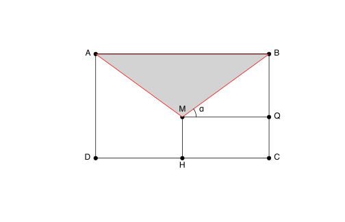
10.2- \(M\) lies on the perpendicular bisector of \([DC]\) (which is also that of \([AB]\)), so \(MA = MB\) and \(MQ = AB/2 = 5\). In the right triangle \(MQB\), \(\cos\alpha = MQ/MB\) and \(\tan\alpha = BQ/MQ\), and \(MH = QC = BC - BQ\):
\begin{equation*} \begin{aligned} MB &= MA = \frac{5}{\cos\alpha}, \qquad BQ = 5\tan\alpha, \qquad MH = 6 - 5\,\frac{\sin\alpha}{\cos\alpha},\\ g(\alpha) &= \frac{10}{\cos\alpha} - \frac{5\sin\alpha}{\cos\alpha} + 6 = \frac{5(2 - \sin\alpha)}{\cos\alpha} + 6 . \end{aligned} \end{equation*}
10.3- and 10.4- The one-dimensional minimizer optimize() of Section 10.5 does it; the search interval is the admissible range \(\left]0; \arctan(6/5)\right]\):
g <- function(alpha) 5 * (2 - sin(alpha)) / cos(alpha) + 6
optimize(g, lower = 0, upper = atan(6/5))
c(pi/6, 6 + 5 * sqrt(3))
$minimum
[1] 0.5235997
$objective
[1] 14.66025
[1] 0.5235988 14.6602540
The minimum is \(g \approx 14.660\), reached at \(\alpha \approx 0.5236\), which matches \(\pi/6\) and \(6 + 5\sqrt{3}\) (the last line).
10.5- By the quotient rule,
\begin{equation*} \begin{aligned} g^{\prime}(\alpha) &= 5\,\frac{-\cos\alpha\cos\alpha + (2 - \sin\alpha)\sin\alpha}{\cos^2\alpha} = 5\,\frac{2\sin\alpha - (\sin^2\alpha + \cos^2\alpha)}{\cos^2\alpha}\\ &= \frac{5(2\sin\alpha - 1)}{\cos^2\alpha}, \end{aligned} \end{equation*}
which is negative then positive, vanishing only at \(\sin\alpha = 1/2\), i.e. \(\alpha = \pi/6\).
10.6- The symbolic derivative from D() (Section 10.4.1):
D(expression(5 * (2 - sin(alpha)) / cos(alpha) + 6), "alpha")
-(5 * cos(alpha)/cos(alpha) - 5 * (2 - sin(alpha)) * sin(alpha)/cos(alpha)^2)
This is \(-5 + 5(2\sin\alpha - \sin^2\alpha)/\cos^2\alpha = 5(2\sin\alpha - \sin^2\alpha - \cos^2\alpha)/\cos^2\alpha\), which simplifies to the result of 10.5.
10.7- The function, checked against the gradient returned by deriv() on a grid of angles:
gprime <- function(alpha) 5 * (2 * sin(alpha) - 1) / cos(alpha)^2
dg <- deriv(~ 5 * (2 - sin(alpha)) / cos(alpha) + 6, "alpha",
function.arg = TRUE)
a <- seq(0.1, 0.8, by = 0.1)
all.equal(as.vector(attr(dg(a), "gradient")), gprime(a))
[1] TRUE
10.8- uniroot() finds the root of gprime on the same interval:
r <- uniroot(gprime, lower = 0, upper = atan(6/5), tol = 1e-10)
c(root = r$root, g.root = g(r$root), diff = r$root - pi/6)
root g.root diff
5.235988e-01 1.466025e+01 1.110223e-16
The root is \(\alpha = \pi/6\) to machine precision and \(g\) there equals \(14.66025\), the same argument and minimum value as optimize() gave in 10.4.
Worksheet 10.W.C — Standard normal table
Worksheet 10.W.C — Standard normal table — Standard normal table
We shall use the function integrate() to create a table for the distribution \(\mathcal{N}(0,1)\).
Let \(\Phi(x)=\int_{-\infty}^{x}\frac{1}{\sqrt{2\pi}}e^{-t^2/2}\,dt\) be the cumulative distribution function of \(\mathcal{N}(0,1)\). It is well known that \(\Phi(-x)=1-\Phi(x)\). We shall thus only create the table for positive values of \(x\).
10.1- Create a function phi() which takes as input a vector \(x\) of length \(n\) and returns the vector of values \(\frac{1}{\sqrt{2\pi}}e^{-x_i^2/2}\), \(i=1,\dots,n\).
10.2- Use the function integrate() to compute \(\Phi(x)\) for all \(x\) in the following vector: quantiles <- seq(0,5.5,by=0.1). Store these values in a vector called probs.
10.3- Use the function all.equal() to compare these results with those given by the function pnorm().
10.4- Plot the values of \(\Phi(x)\) for all \(x\) and all \(-x\) in quantiles (hint: use the function rev()).
10.5- Plot the function pnorm() in blue over the previous curve. Check that the two plots coincide perfectly.
10.1- Vectorised arithmetic makes phi() a one-liner:
phi <- function(x) exp(-x^2/2) / sqrt(2*pi)
phi(c(0, 1, 2))
[1] 0.39894228 0.24197072 0.05399097
10.2- integrate() takes a single upper bound, so we loop over quantiles with sapply() and keep the $value component:
quantiles <- seq(0, 5.5, by = 0.1)
probs <- sapply(quantiles, function(q) integrate(phi, -Inf, q)$value)
head(round(probs, 4))
tail(round(probs, 7), 3)
[1] 0.5000 0.5398 0.5793 0.6179 0.6554 0.6915
[1] 0.9999999 1.0000000 1.0000000
These are the familiar table entries \(\Phi(0)=0.5\), \(\Phi(0.5)=0.6915\), and so on.
10.3- The numerical integrals agree with pnorm() to within all.equal()’s default tolerance (\(1.5\times 10^{-8}\)); the largest absolute discrepancy is about \(4.6\times10^{-9}\):
all.equal(probs, pnorm(quantiles))
max(abs(probs - pnorm(quantiles)))
[1] TRUE
[1] 4.559252e-09
10.4- By symmetry \(\Phi(-x)=1-\Phi(x)\), so the negative half is 1 - rev(probs). We drop the duplicated point \(x=0\) with [-1]:
x <- c(-rev(quantiles[-1]), quantiles)
Phi <- c(1 - rev(probs[-1]), probs)
plot(x, Phi, type = "l", lwd = 4, col = "grey",
xlab = "x", ylab = expression(Phi(x)))
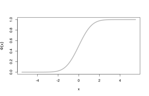
10.5- We draw pnorm() in thin blue over the thick grey curve with curve(..., add = TRUE). The blue line runs exactly along the grey one, and all.equal() confirms this over all 111 points:
plot(x, Phi, type = "l", lwd = 4, col = "grey",
xlab = "x", ylab = expression(Phi(x)))
curve(pnorm(x), add = TRUE, col = "blue", lwd = 1.5)
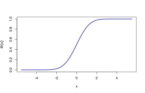
all.equal(Phi, pnorm(x))
[1] TRUE
Worksheet 10.W.D — Principal components analysis
Worksheet 10.W.D — Principal components analysis — Bordeaux climate and wine quality
Principal components analysis is used to describe the proximity of individuals on which several quantitative traits have been measured. This method requires many matrix operations, and is thus a good way to put into practice the notions introduced at the beginning of this chapter.
Data were collected in the wine region of Bordeaux. They include:
- four weather traits:
TEMPER(sum of daily average temperatures, in degrees Celsius),SUN(length of insolation, in hours),HEAT(number of days of strong heat),RAIN(rainfall, in mm); - wine quality (
QUALITY), as determined by wine-tasters: 1 = good wine, 2 = average wine, 3 = mediocre wine.
We shall represent these quantitative data on a scatter plot after projecting the data onto a subspace (a plane) chosen so as to limit the loss of information caused by the projection.
10.1- Import into the variable climatewine the contents of the data file http://www.biostatisticien.eu/springeR/climatewine.csv
10.2- Store in matrix X the variables TEMPER, SUN, HEAT, RAIN (hint: as.matrix()).
10.3- Calculate the centre (of gravity) g of the scatter plot of individuals included in X (vector of column averages) with the function colMeans(). Display it with two decimal places.
10.4- Use the function scale() to calculate the matrix \(\dot{X} = (\dot{x}_{ij})\) of centred data, and store it in the variable Xdot.
10.5- Calculate the global inertia of the scatter plot, which represents the dispersion of the points: \(I = \frac{1}{n}\sum_{i=1}^{n}\sum_{j=1}^{n}\dot{x}_{ij}^{2}\), where \(n\) is the number of individuals in \(X\).
10.6- The contribution of individual \(i\) to the global inertia is given by the formula \(\frac{1}{nI}\sum_{j=1}^{p}\dot{x}_{ij}^{2}\), where \(p\) is the number of variables (four in this case). Calculate the vector inertiacontr of contributions to inertia from each individual.
10.7- Create the column matrix onen of length \(n\), containing only 1’s.
10.8- Check that the centre of gravity g of the scatter plot is also given by the formula \(g = \frac{1}{n}X^{T}1_n\).
10.9- Check that the matrix Xdot of centred data is also given by the formula \(\dot{X} = X - 1_n g^{T}\).
10.10- Calculate the matrix of covariances S with the formula \(S = \frac{1}{n}\dot{X}^{T}\dot{X}\). Try to reproduce this result with the function cov().
10.11- Use the matrix S to calculate the diagonal matrix Doneovers containing the inverses of standard deviations: \(D_{1/s} = \mathrm{diag}(1/s_1, \ldots, 1/s_p)\).
10.12- Calculate the matrix Z of scaled and centred data with the formula \(Z = \dot{X}D_{1/s}\).
10.13- Calculate the matrix of correlations R with the formula \(R = \frac{1}{n}Z^{T}Z\). Try to reproduce this result with the function cor().
10.14- Calculate the diagonal matrix Lambda of eigenvalues (\(\Lambda\)) and the matrix W of eigenvectors (\(W\)) of the correlation matrix \(R\). The matrix W contains the coordinates of a new basis in which we shall represent the individuals.
10.15- Plot the circle of correlations, which is a circle of radius 1, over which you should overlay arrows starting at the origin and ending at the points with coordinates given by the first two columns of the matrix \(W\Lambda^{1/2}\). On the same plot, add the names of the variables at the end of the four arrows.
10.16- The total inertia of the scaled and centred scatter plot is equal to the number of variables (four in this case). It can be decomposed into a sum of inertias contributed by each one of the four axes of the basis of \(W\), which are given by the diagonal of \(\Lambda\). Calculate the vector of percentages of total inertia explained by the first \(k\) axes (\(1 \le k \le p\)). What percentage of the inertia is explained by the first two axes?
10.17- Calculate the matrix CW of principal components with the formula \(C_W = ZW\). The principal components are the coordinates of the individuals in the new basis described by W.
10.18- Open a new graphics window and plot the individuals projected onto the first principal plane, i.e. with coordinates given by the first two columns of \(C_W\). Add the names of the individuals onto the plot.
10.19- Draw the last plot again, but this time plot in red (respectively blue, green) good wines (respectively average wines, mediocre wines). Add a caption.
10.20- The quality of representation of individual \(i\) on the first principal plane is given by the formula \(\frac{c_{i1}^{2}+c_{i2}^{2}}{\sum_{j=1}^{p}c_{ij}^{2}}\), where \(c_{ij}\) is the entry at row \(i\) and column \(j\) of the matrix \(C_W\). Calculate the vector QLT of qualities of representation of individuals on the first principal plane. Display QLT with two decimal places.
10.21- We shall briefly explore package ade4 which performs PCA. Install and load this package.
10.22- Type the following instructions:
rownames(X) <- climatewine[,1]
res <- dudi.pca(X) # Answer 2 to the question you are asked.
scatter(res)
s.class(res$li,as.factor(climatewine[,6]))
10.1- The file is tab-separated with a header line, so read.table() with header = TRUE reads it directly from the URL (34 years, 1924-1957).
climatewine <- read.table("http://www.biostatisticien.eu/springeR/climatewine.csv",
header = TRUE)
head(climatewine, 3)
dim(climatewine)
YEAR TEMPER SUN HEAT RAIN QUALITY
1 1924 3064 1201 10 361 2
2 1925 3000 1053 11 338 3
3 1926 3155 1133 19 393 2
[1] 34 6
10.2- Select the four weather columns and coerce with as.matrix().
X <- as.matrix(climatewine[, c("TEMPER", "SUN", "HEAT", "RAIN")])
n <- nrow(X); p <- ncol(X)
10.3- The centre of gravity is the vector of column means.
g <- colMeans(X)
round(g, 2)
TEMPER SUN HEAT RAIN
3157.88 1247.32 18.82 360.44
10.4- scale() with scale = FALSE only subtracts the column means.
Xdot <- scale(X, center = TRUE, scale = FALSE)
10.5- The inner sum runs over the \(p\) variables, not \(n\) (the printed upper limit \(n\) on \(j\) is a typo): \(I = \frac{1}{n}\sum_{i=1}^{n}\sum_{j=1}^{p}\dot{x}_{ij}^{2}\).
inertia <- sum(Xdot^2) / n
inertia
[1] 43114.48
The unscaled inertia is dominated by TEMPER and SUN, whose variances are in the tens of thousands.
10.6- Row sums of squares divided by \(nI\); the contributions add to 1.
inertiacontr <- rowSums(Xdot^2) / (n * inertia)
round(head(inertiacontr), 4)
sum(inertiacontr)
[1] 0.0075 0.0432 0.0096 0.0640 0.0085 0.0339
[1] 1
10.7- A one-column matrix of 1’s:
onen <- matrix(1, nrow = n, ncol = 1)
10.8- The matrix product \(\frac{1}{n}X^{T}1_n\) returns the same vector as colMeans().
all.equal(g, drop(t(X) %*% onen / n))
[1] TRUE
10.9- The outer product \(1_n g^{T}\) repeats g on each row; check.attributes = FALSE ignores the "scaled:center" attribute that scale() attaches.
all.equal(Xdot, X - onen %*% t(g), check.attributes = FALSE)
[1] TRUE
10.10- \(S = \frac{1}{n}\dot{X}^{T}\dot{X}\) uses divisor \(n\), whereas cov() uses \(n-1\), so cov(X) must be rescaled by \((n-1)/n\) to match.
S <- t(Xdot) %*% Xdot / n
round(S, 1)
all.equal(S, cov(X) * (n - 1) / n, check.attributes = FALSE)
TEMPER SUN HEAT RAIN
TEMPER 19346.8 12360.3 1187.4 -5130.4
SUN 12360.3 15561.8 795.8 -5317.8
HEAT 1187.4 795.8 97.4 -356.5
RAIN -5130.4 -5317.8 -356.5 8108.5
[1] TRUE
10.11- The standard deviations are the square roots of the diagonal of S; diag() builds the diagonal matrix of their inverses.
Doneovers <- diag(1 / sqrt(diag(S)))
round(Doneovers, 5)
[,1] [,2] [,3] [,4]
[1,] 0.00719 0.00000 0.00000 0.00000
[2,] 0.00000 0.00802 0.00000 0.00000
[3,] 0.00000 0.00000 0.10134 0.00000
[4,] 0.00000 0.00000 0.00000 0.01111
10.12- Right-multiplying by \(D_{1/s}\) divides each centred column by its standard deviation.
Z <- Xdot %*% Doneovers
colnames(Z) <- colnames(X)
10.13- \(R = \frac{1}{n}Z^{T}Z\) coincides with cor(X) (the \(n\) versus \(n-1\) divisor cancels in a correlation).
R <- t(Z) %*% Z / n
round(R, 3)
all.equal(R, cor(X), check.attributes = FALSE)
TEMPER SUN HEAT RAIN
TEMPER 1.000 0.712 0.865 -0.410
SUN 0.712 1.000 0.646 -0.473
HEAT 0.865 0.646 1.000 -0.401
RAIN -0.410 -0.473 -0.401 1.000
[1] TRUE
The three heat-related traits are strongly positively correlated with one another and negatively with rainfall.
10.14- eigen() returns the eigenvalues in decreasing order and the unit eigenvectors in columns (each defined only up to sign).
eig <- eigen(R)
Lambda <- diag(eig$values)
W <- eig$vectors
dimnames(W) <- list(colnames(X), paste0("Axis", 1:p))
round(diag(Lambda), 4)
round(W, 3)
[1] 2.7915 0.7145 0.3659 0.1281
Axis1 Axis2 Axis3 Axis4
TEMPER -0.550 -0.305 -0.208 0.749
SUN -0.513 -0.008 0.846 -0.146
HEAT -0.537 -0.317 -0.441 -0.646
RAIN 0.382 -0.898 0.218 -0.025
10.15- The first two columns of \(W\Lambda^{1/2}\) are the correlations between each variable and the first two principal components.
coords <- W %*% sqrt(Lambda)
round(coords[, 1:2], 3)
[,1] [,2]
TEMPER -0.920 -0.258
SUN -0.858 -0.007
HEAT -0.896 -0.268
RAIN 0.638 -0.759
theta <- seq(0, 2 * pi, length.out = 200)
plot(cos(theta), sin(theta), type = "l", asp = 1, xlab = "Axis 1",
ylab = "Axis 2", main = "Circle of correlations")
abline(h = 0, v = 0, lty = 3)
arrows(0, 0, coords[, 1], coords[, 2], length = 0.1)
text(coords[, 1], coords[, 2], labels = colnames(X), pos = c(2, 3, 1, 4))
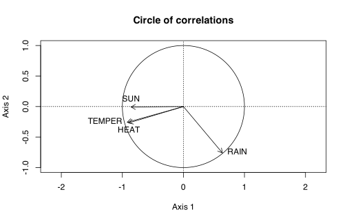
All four arrows reach close to the circle, so the four variables are well represented on the first plane: axis 1 opposes warm, sunny years (TEMPER, SUN, HEAT on the left) to rainy years (RAIN on the right), and axis 2 is driven mainly by RAIN.
10.16- The cumulative sums of the eigenvalues, divided by \(p = 4\):
round(100 * cumsum(diag(Lambda)) / p, 2)
[1] 69.79 87.65 96.80 100.00
The first two axes explain 87.65% of the total inertia, so the first principal plane loses little information.
10.17- The principal components are \(C_W = ZW\); the variance (divisor \(n\)) of column \(k\) equals the \(k\)-th eigenvalue.
CW <- Z %*% W
round(head(CW, 3), 3)
round(apply(CW, 2, var) * (n - 1) / n, 4)
Axis1 Axis2 Axis3 Axis4
[1,] 1.044 0.487 0.222 0.126
[2,] 1.755 0.835 -0.787 -0.104
[3,] 0.610 -0.316 -0.700 0.098
Axis1 Axis2 Axis3 Axis4
2.7915 0.7145 0.3659 0.1281
10.18- Open a new device with dev.new() (or x11()=/=quartz()=/=windows()) and label each point with its year.
dev.new()
plot(CW[, 1], CW[, 2], type = "n", asp = 1, xlab = "Axis 1", ylab = "Axis 2",
main = "Individuals on the first principal plane")
abline(h = 0, v = 0, lty = 3)
text(CW[, 1], CW[, 2], labels = climatewine$YEAR, cex = 0.8)
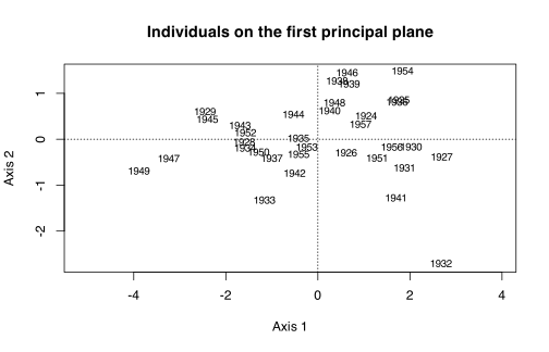
Years on the left (e.g. 1947, 1949) were hot and sunny; years on the right (e.g. 1927, 1932) were cool and wet.
10.19- Index a colour vector by QUALITY and add a legend.
cols <- c("red", "blue", "green")[climatewine$QUALITY]
plot(CW[, 1], CW[, 2], type = "n", asp = 1, xlab = "Axis 1", ylab = "Axis 2",
main = "Individuals coloured by wine quality")
abline(h = 0, v = 0, lty = 3)
text(CW[, 1], CW[, 2], labels = climatewine$YEAR, col = cols, cex = 0.8)
legend("topright", legend = c("good", "average", "mediocre"),
text.col = c("red", "blue", "green"), title = "Quality",
title.col = "black", bty = "n")
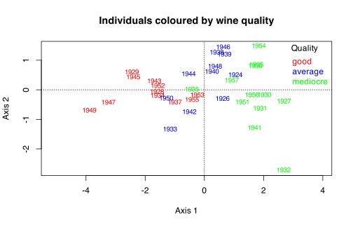
Quality follows the first axis: good vintages sit on the hot, sunny left, mediocre ones on the cool, rainy right, and average ones in between.
10.20- Squared coordinates on axes 1-2 divided by the squared distance to the origin across all four axes:
QLT <- rowSums(CW[, 1:2]^2) / rowSums(CW^2)
names(QLT) <- climatewine$YEAR
round(QLT, 2)
names(QLT)[QLT < 0.6]
1924 1925 1926 1927 1928 1929 1930 1931 1932 1933 1934 1935 1936 1937 1938 1939
0.95 0.86 0.49 0.83 0.65 0.94 0.67 0.89 0.99 0.99 0.95 0.13 0.97 0.52 0.87 0.76
1940 1941 1942 1943 1944 1945 1946 1947 1948 1949 1950 1951 1952 1953 1954 1955
0.32 0.88 0.76 0.95 0.77 0.93 0.97 0.86 0.78 1.00 0.95 0.96 0.91 0.86 0.96 0.61
1956 1957
0.81 0.91
[1] "1926" "1935" "1937" "1940"
Most years are well represented on the plane; the positions of 1926, 1935, 1937 and 1940 (quality below 0.6, 1935 only 0.13) should not be interpreted from this plot.
10.21- Install once from CRAN with install.packages("ade4"), then load it in each session.
# install.packages("ade4") # only once per R installation
library(ade4)
10.22- dudi.pca() centres and scales by default, so it reproduces our eigenvalues; answering 2 to its interactive question keeps two axes, which is what scannf = FALSE, nf = 2 does non-interactively.
rownames(X) <- climatewine[, 1]
res <- dudi.pca(X, scannf = FALSE, nf = 2)
round(res$eig, 4)
all.equal(abs(as.matrix(res$li)), abs(CW[, 1:2]), check.attributes = FALSE)
all.equal(abs(as.matrix(res$co)), abs(coords[, 1:2]), check.attributes = FALSE)
[1] 2.7915 0.7145 0.3659 0.1281
[1] TRUE
[1] TRUE
res$li (row coordinates) is \(C_W\) and res$co (column coordinates) is \(W\Lambda^{1/2}\), up to the sign of each axis. scatter(res) draws the biplot (individuals plus variable arrows):
scatter(res)
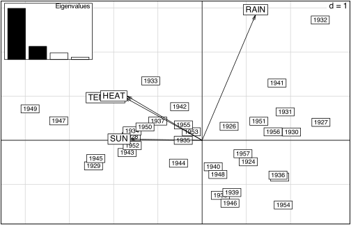
s.class() draws the individuals grouped by quality, with each group’s centre of gravity and inertia ellipse:
s.class(res$li, as.factor(climatewine[, 6]))
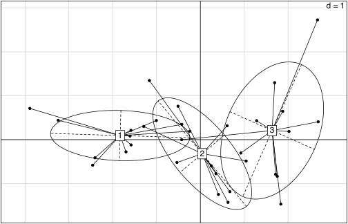
The three quality groups (1 = good, 2 = average, 3 = mediocre) are ordered along the first axis with only partial overlap of their ellipses, confirming that the climate traits largely separate the vintages by quality.
Descriptive statistics
Exercises 11.1–11.7
Give the instruction which returns the table of frequencies for a qualitative variable x.
table(x)/length(x) (equivalently prop.table(table(x))), as in Section 11.3.2; here x is the variable fat of the nutrition_elderly data used throughout the chapter (gdata::read.xls() no longer exists in current gdata, so the file is read with readxl).
library(readxl)
f <- tempfile(fileext = ".xls")
download.file("http://www.biostatisticien.eu/springeR/nutrition_elderly.xls",
f, mode = "wb", quiet = TRUE)
NE <- as.data.frame(read_excel(f))
gender <- factor(NE$gender, labels = c("Male", "Female"))
fat <- factor(NE$fat, labels = c("butter", "margarine", "peanut",
"sunflower", "olive", "Isio4", "rapeseed", "duck"))
weight <- NE$weight; height <- NE$height; tea <- NE$tea
x <- fat
round(table(x)/length(x), 3)
x
butter margarine peanut sunflower olive Isio4 rapeseed duck
0.066 0.119 0.212 0.301 0.177 0.102 0.004 0.018
Give the instruction which returns the contingency table for qualitative variables x and y.
table(x, y) (Section 11.3.4.1); with x = gender and y = fat:
genderfat <- table(gender, fat)
genderfat
fat
gender butter margarine peanut sunflower olive Isio4 rapeseed duck
Male 10 10 16 21 20 5 0 3
Female 5 17 32 47 20 18 1 1
Which function returns the marginal distributions from a contingency table?
margin.table(), with second argument 1 for the row margin and 2 for the column margin (Section 11.3.4.3).
margin.table(genderfat, 1)
margin.table(genderfat, 2)
gender
Male Female
85 141
fat
butter margarine peanut sunflower olive Isio4 rapeseed duck
15 27 48 68 40 23 1 4
Which function returns the conditional distributions from a contingency table?
prop.table(), with margin = 1 for the distributions conditional on the rows (row profiles) and margin = 2 for those conditional on the columns (Section 11.3.4.4).
round(prop.table(genderfat, 1), 3)
fat
gender butter margarine peanut sunflower olive Isio4 rapeseed duck
Male 0.118 0.118 0.188 0.247 0.235 0.059 0.000 0.035
Female 0.035 0.121 0.227 0.333 0.142 0.128 0.007 0.007
Give the instruction which returns the mode of a distribution.
names(which.max(table(x))) returns a (the first) mode; names(tab)[tab = max(tab)]= with tab <- table(x) returns all of them when there are ties (Section 11.4.1.1). For the number of cups of tea per day, the mode is 0 cups:
tabtea <- table(tea)
names(which.max(tabtea))
names(tabtea)[tabtea == max(tabtea)]
[1] "0"
[1] "0"
Give the instruction which returns the range of a vector x.
diff(range(x)) (or max(x) - min(x)); note that range(x) alone returns the pair (minimum, maximum), not the range (Section 11.4.2). For the heights:
x <- height
range(x)
diff(range(x))
[1] 140 188
[1] 48
Give the instruction which returns the interquartile range of a vector x.
IQR(x), i.e. \(q_{3/4} - q_{1/4}\) (Section 11.4.2).
IQR(x)
[1] 13
Exercises 11.8–11.14
Give the instruction which returns the (non empirical) variance of a vector x.
var(x) * (length(x) - 1) / length(x), the book’s var.pop(x): the variance \(\sigma^2_{\text{Pop}}\) of the population, with divisor \(N\) (Section 11.4.2); var(x) alone is the unbiased sample estimator with divisor \(n-1\) (Note in Section 11.4.2).
var(x) * (length(x) - 1) / length(x)
var(x)
[1] 80.70195
[1] 81.06063
Give the code of a function which calculates the coefficient of variation.
The coefficient of variation is \(cv = \sigma_{\text{Pop}}/\mu_X\) (Section 11.4.2):
co.var <- function(x) {
sd.pop <- sqrt(mean((x - mean(x))^2))
sd.pop / mean(x)
}
co.var(x)
[1] 0.0547903
Give the instruction which calculates the mean absolute deviation.
mean(abs(x - mean(x))), i.e. \(\frac{1}{N}\sum_{i=1}^N |x_i - \bar{x}|\) (Section 11.4.2; not to be confused with mad(), the median absolute deviation).
mean(abs(x - mean(x)))
[1] 7.312045
Which package includes functions to calculate skewness and kurtosis?
The package moments, through its functions skewness() and kurtosis() (Section 11.4.3); they return \(\gamma_1\) and \(\beta_2\) exactly as the book’s skew() and kurt().
library(moments)
skewness(x)
kurtosis(x)
[1] 0.4256203
[1] 2.778185
Give the instruction which returns Cramér’s \(\Phi^2\).
chisq.test(tab, correct = FALSE)$statistic/sum(tab) (correct = FALSE stops a Yates correction on a 2 x 2 table), i.e. \(\Phi^2 = \chi^2/N\) for a contingency table tab (Section 11.5.1.2). For gender by fat:
chi2 <- suppressWarnings(chisq.test(genderfat, correct = FALSE))$statistic
Phi2 <- unname(chi2 / sum(genderfat))
Phi2
[1] 0.06707265
Give the code of a function which calculates the correlation ratio \(\eta^2_{Y|X}\).
The function below computes \(\eta^2_{Y|X} = \sum_k n_k(\bar{y}_k - \bar{y})^2 / \sum_i (y_i - \bar{y})^2\) (Section 11.5.4.1):
eta2 <- function(y, gpe) {
means <- tapply(y, gpe, mean)
counts <- tapply(y, gpe, length)
sum(counts * (means - mean(y))^2) / sum((y - mean(y))^2)
}
eta2(weight, gender)
[1] 0.3325501
So gender accounts for about 33% of the variation in weight.
Which function would you use to draw a Pareto chart?
barplot() applied to the sorted table of counts, barplot(sort(table(x), decreasing = TRUE)) (Section 11.6.1.3).
Exercises 11.15–11.18
Which function would you use to draw a stacked bar chart?
barplot() with a matrix as its first argument (one column per bar, e.g. the cbind() of the frequency tables of each group), since beside = FALSE is the default (Section 11.6.1.4).
Which function would you use to draw a pie chart?
pie(), applied to a table of counts, e.g. pie(table(x)) (Section 11.6.1.5).
Which function would you use to draw a box plot?
boxplot(), e.g. boxplot(x), or boxplot(y ~ g) for one box per level of a factor g (Sections 11.6.3.5 and 11.6.4.3).
Which function would you use to draw a histogram?
hist(), with breaks to set the class boundaries and freq = FALSE for a density histogram (Section 11.6.4.4).
Worksheet 11.W.A — Thoughts on independence in descriptive statistics
Worksheet 11.W.A — Descriptive data studies — Thoughts on independence in descriptive statistics
11.1- Import the file http://www.biostatisticien.eu/springeR/snee74en.txt into an R object called snee.
11.2- Display the first and last lines of snee with the functions head() and tail(). How many individuals are there? How many variables? What type are the variables?
11.3- Use the function attach() on your data.frame then check with the functions class() and levels() that the structure of your variables is correct. What are the levels of the variables?
11.4- Perform a univariate descriptive study of each variable: numerical results and appropriate graphical representations.
11.5- We shall now study the dependence of variables eyes and hair. Create the contingency table eyeshair (observed counts) of variables eyes and hair.
11.6- Calculate the frequency of each level of the variable hair (profile by column). You get the distribution function fhair of hair colour in the population.
11.7- Now, include the second characteristic: eye colour. Calculate the number nblue of individuals with blue eyes in the entire population.
11.8- Suppose that eye colour and hair colour are independent. In other words, the fact that an individual has blue eyes bears no relation with the colour of their hair. In that case, the proportions calculated in 11.6 should still be the same within the subpopulation of people with blue eyes. Under this independence hypothesis, calculate the number of blue-eyed people who should have blond hair (respectively brown, black and red).
11.9- Do the same with other eye colours. You get a table tab.ind1 of theoretical counts under the hypothesis of independence between eye and hair colour.
11.10- Repeat the entire process, but with the two characteristics inverted (i.e. start with the variable eyes). From table eyeshair, calculate the frequency of each level of the variable eyes (profiles by rows). You get the distribution function feyes of eye colours in the population.
11.11- Now include the second characteristic: hair colour. Calculate the number nblond of people with blond hair in the entire population.
11.12- Suppose that hair and eye colour are independent. In other words, the fact that an individual has blond hair bears no relation with their eye colour. In that case, the proportions calculated in 11.10 should still be the same within the subpopulation of people with blond hair. Under this independence hypothesis, calculate the number of blond people who should have blue eyes (respectively brown, hazel and green).
11.13- Do the same with other hair colours. You get a table tab.ind2 of theoretical counts under the hypothesis of independence between hair and eye colour.
11.14- Use the function all.equal() to compare the two tables of theoretical counts. What do you observe?
11.15- Compare the table of observed counts eyeshair with the table of theoretical counts (for each entry, calculate the square of the difference).
11.16- Calculate the table of contributions to the \(\chi^2\).
11.17- Calculate all relevant link indicators. Conclude.
11.18- Independence can also be defined (and this is in fact the primary definition) as equality of all conditional distributions. Calculate the conditional distribution of the variable hair knowing that the eye colour is blue (i.e. the frequency of various hair colours knowing that eye colour is blue). Calculate the three other conditional distributions of the variable hair. Calculate the conditional distributions of the variable eyes knowing each of the levels of variable hair. Conclude.
11.19- Perform a descriptive study of variable hair as a function of variable gender.
11.20- Perform a descriptive study of variable eyes as a function of variable gender.
11.21- Analyze the dependence between eye colour and hair colour for the following contingency table (rows: Eyes; columns: Hair):
| Eyes | Blond | Brown | Black | Red | Total |
|---|---|---|---|---|---|
| Blue | 1768 | 807 | 189 | 47 | 2811 |
| Grey/green | 946 | 1387 | 746 | 53 | 3132 |
| Brown | 115 | 438 | 288 | 16 | 857 |
| Total | 2829 | 2632 | 1223 | 116 | 6800 |
11.1- Use read.table() with header = TRUE; since R 4.0 strings are no longer converted to factors by default, so add stringsAsFactors = TRUE to get the qualitative variables as factors.
snee <- read.table("http://www.biostatisticien.eu/springeR/snee74en.txt",
header = TRUE, stringsAsFactors = TRUE)
11.2- There are 592 individuals and 3 variables (hair, eyes, gender), all qualitative (nominal), stored as factors.
head(snee)
tail(snee)
dim(snee)
hair eyes gender
1 Black Brown Male
2 Blond Blue Female
3 Black Blue Male
4 Brown Brown Female
5 Red Brown Male
6 Brown Blue Male
hair eyes gender
587 Black Brown Male
588 Blond Brown Female
589 Brown Blue Male
590 Brown Hazel Male
591 Brown Hazel Female
592 Brown Blue Male
[1] 592 3
11.3- All three variables are factors, which is the correct structure for nominal data; hair has levels Black, Blond, Brown, Red, eyes has Blue, Brown, Green, Hazel, and gender has Female, Male.
attach(snee)
sapply(snee, class)
levels(hair); levels(eyes); levels(gender)
hair eyes gender
"factor" "factor" "factor"
[1] "Black" "Blond" "Brown" "Red"
[1] "Blue" "Brown" "Green" "Hazel"
[1] "Female" "Male"
11.4- For nominal variables the numerical summaries are the counts (summary()) and relative frequencies (prop.table(table())), and the appropriate graphics are Pareto/bar charts and pie charts (Section 11.6.1).
summary(snee)
lapply(snee, function(v) round(prop.table(table(v)), 3))
hair eyes gender
Black:108 Blue :215 Female:328
Blond:127 Brown:220 Male :264
Brown:286 Green: 64
Red : 71 Hazel: 93
$hair
v
Black Blond Brown Red
0.182 0.215 0.483 0.120
$eyes
v
Blue Brown Green Hazel
0.363 0.372 0.108 0.157
$gender
v
Female Male
0.554 0.446
par(mfrow = c(1, 3))
barplot(sort(table(hair), decreasing = TRUE), main = "hair", col = "grey",
cex.names = 0.8)
barplot(sort(table(eyes), decreasing = TRUE), main = "eyes", col = "grey",
cex.names = 0.8)
pie(table(gender), main = "gender", col = c("pink", "lightblue"))
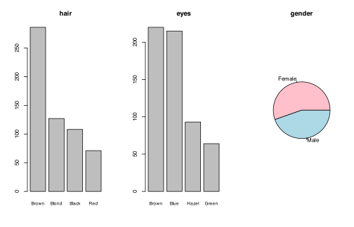
Brown is the modal hair colour (48.3%) and red the rarest (12.0%); brown and blue eyes dominate (37.2% and 36.3%), green is rare (10.8%); the sample is 55.4% female.
11.5- The observed contingency table (with margins from addmargins()):
eyeshair <- table(eyes, hair)
addmargins(eyeshair)
hair
eyes Black Blond Brown Red Sum
Blue 20 94 84 17 215
Brown 68 7 119 26 220
Green 5 16 29 14 64
Hazel 15 10 54 14 93
Sum 108 127 286 71 592
11.6- fhair is the column margin divided by the total:
fhair <- margin.table(eyeshair, 2) / sum(eyeshair)
round(fhair, 4)
hair
Black Blond Brown Red
0.1824 0.2145 0.4831 0.1199
11.7- There are nblue = 215 blue-eyed individuals.
nblue <- sum(eyeshair["Blue", ]); nblue
[1] 215
11.8- Under independence the 215 blue-eyed people split like the whole population: about 46.1 blond, 103.9 brown, 39.2 black and 25.8 red-haired.
nblue * fhair
hair
Black Blond Brown Red
39.22297 46.12331 103.86824 25.78547
11.9- Repeating for every eye colour amounts to the outer product of the eye-colour counts with fhair:
neyes <- margin.table(eyeshair, 1)
tab.ind1 <- outer(neyes, fhair)
round(tab.ind1, 2)
hair
eyes Black Blond Brown Red
Blue 39.22 46.12 103.87 25.79
Brown 40.14 47.20 106.28 26.39
Green 11.68 13.73 30.92 7.68
Hazel 16.97 19.95 44.93 11.15
11.10- feyes is the row margin divided by the total:
feyes <- margin.table(eyeshair, 1) / sum(eyeshair)
round(feyes, 4)
eyes
Blue Brown Green Hazel
0.3632 0.3716 0.1081 0.1571
11.11- There are nblond = 127 blond-haired individuals.
nblond <- sum(eyeshair[, "Blond"]); nblond
[1] 127
11.12- Under independence the 127 blond people should comprise about 46.1 blue-eyed, 47.2 brown-eyed, 20.0 hazel-eyed and 13.7 green-eyed people.
nblond * feyes
eyes
Blue Brown Green Hazel
46.12331 47.19595 13.72973 19.95101
11.13- Repeating for every hair colour gives the outer product of feyes with the hair-colour counts:
nhair <- margin.table(eyeshair, 2)
tab.ind2 <- outer(feyes, nhair)
round(tab.ind2, 2)
hair
eyes Black Blond Brown Red
Blue 39.22 46.12 103.87 25.79
Brown 40.14 47.20 106.28 26.39
Green 11.68 13.73 30.92 7.68
Hazel 16.97 19.95 44.93 11.15
11.14- The two tables are identical: both equal \(E_{ij} = n_{i\cdot}\,n_{\cdot j}/N\), which is symmetric in the two variables, and they coincide with the expected counts returned by chisq.test() (Section 11.5.1).
all.equal(tab.ind1, tab.ind2)
all.equal(tab.ind1, chisq.test(eyeshair)$expected, check.attributes = FALSE)
[1] TRUE
[1] TRUE
11.15- The squared differences \((O_{ij}-E_{ij})^2\) are largest for blond hair (blue eyes: far more than expected; brown eyes: far fewer) and for black hair with brown eyes:
round((eyeshair - tab.ind1)^2, 2)
hair
eyes Black Blond Brown Red
Blue 369.52 2292.18 394.75 77.18
Brown 776.45 1615.71 161.70 0.15
Green 44.56 5.15 3.68 40.00
Hazel 3.87 99.02 82.28 8.10
11.16- The contributions are \((O_{ij}-E_{ij})^2/E_{ij}\), i.e. the squared Pearson residuals of chisq.test():
tab.contr <- (eyeshair - tab.ind1)^2 / tab.ind1
round(tab.contr, 2)
all.equal(c(tab.contr), c(chisq.test(eyeshair)$residuals^2))
hair
eyes Black Blond Brown Red
Blue 9.42 49.70 3.80 2.99
Brown 19.35 34.23 1.52 0.01
Green 3.82 0.38 0.12 5.21
Hazel 0.23 4.96 1.83 0.73
[1] TRUE
The cells blond/blue (49.7), blond/brown (34.2) and black/brown (19.4) alone account for 75% of the total \(\chi^2\).
11.17- With \(\chi^2 = 138.3\), \(\Phi^2 = 0.234\), Cramér’s \(V^2 = 0.078\) and Pearson’s \(C = 0.435\) (formulas of Section 11.5.1.2), eye and hair colour are clearly associated.
chi2 <- sum(tab.contr)
N <- sum(eyeshair); p <- nrow(eyeshair); q <- ncol(eyeshair)
Phi2 <- chi2 / N
c(chi2 = chi2, Phi2 = Phi2, V2 = Phi2 / (min(p, q) - 1),
C = sqrt(chi2 / (N + chi2)))
chisq.test(eyeshair)
chi2 Phi2 V2 C
138.2898416 0.2335977 0.0778659 0.4351585
Pearson's Chi-squared test
data: eyeshair
X-squared = 138.29, df = 9, p-value < 2.2e-16
The association is of moderate strength (\(C = 0.435\) against a maximum of \(\sqrt{3/4} \approx 0.866\) for a \(4\times 4\) table), and the test of independence (\(H_0\): eye and hair colour independent, 9 df) is rejected with \(p < 2.2\times 10^{-16}\).
11.18- prop.table(eyeshair, 1) gives the four conditional distributions of hair given each eye colour (row profiles), and prop.table(eyeshair, 2) those of eyes given each hair colour (column profiles):
round(prop.table(eyeshair, 1), 3)
round(prop.table(eyeshair, 2), 3)
hair
eyes Black Blond Brown Red
Blue 0.093 0.437 0.391 0.079
Brown 0.309 0.032 0.541 0.118
Green 0.078 0.250 0.453 0.219
Hazel 0.161 0.108 0.581 0.151
hair
eyes Black Blond Brown Red
Blue 0.185 0.740 0.294 0.239
Brown 0.630 0.055 0.416 0.366
Green 0.046 0.126 0.101 0.197
Hazel 0.139 0.079 0.189 0.197
The conditional distributions are far from equal (43.7% of blue-eyed people are blond against 3.2% of brown-eyed people; 74.0% of blonds have blue eyes against 18.5% of black-haired people), so the variables are not independent, in agreement with 11.17.
11.19- Hair colour distributions are very similar in both sexes (brown about 48% in each; women slightly more often blond, 24.7% vs 17.4%, men slightly more often black-haired, 21.2% vs 15.9%), and the link is negligible: \(\Phi^2 = V^2 = 0.0105\), \(C = 0.10\), and the \(\chi^2\) test (3 df) does not reject independence (\(p = 0.10\)).
assoc <- function(tab) {
chi2 <- chisq.test(tab)$statistic; N <- sum(tab)
Phi2 <- chi2 / N
round(c(chi2 = unname(chi2), Phi2 = unname(Phi2),
V2 = unname(Phi2) / (min(dim(tab)) - 1),
C = unname(sqrt(chi2 / (N + chi2)))), 4)
}
gh <- table(gender, hair)
addmargins(gh)
round(prop.table(gh, 1), 3)
assoc(gh)
chisq.test(gh)$p.value
hair
gender Black Blond Brown Red Sum
Female 52 81 158 37 328
Male 56 46 128 34 264
Sum 108 127 286 71 592
hair
gender Black Blond Brown Red
Female 0.159 0.247 0.482 0.113
Male 0.212 0.174 0.485 0.129
chi2 Phi2 V2 C
6.2212 0.0105 0.0105 0.1020
[1] 0.1013296
11.20- Eye colour depends only weakly on gender: women more often have brown eyes (41.8% vs 31.4%), men slightly more often blue, green or hazel eyes; \(V^2 = 0.012\), \(C = 0.11\), and the \(\chi^2\) test (3 df) is not significant at the 5% level (\(p = 0.063\)). The side-by-side bar charts of the row profiles (Section 11.6.5) display both studies.
ge <- table(gender, eyes)
addmargins(ge)
round(prop.table(ge, 1), 3)
assoc(ge)
chisq.test(ge)$p.value
eyes
gender Blue Brown Green Hazel Sum
Female 114 137 31 46 328
Male 101 83 33 47 264
Sum 215 220 64 93 592
eyes
gender Blue Brown Green Hazel
Female 0.348 0.418 0.095 0.140
Male 0.383 0.314 0.125 0.178
chi2 Phi2 V2 C
7.2800 0.0123 0.0123 0.1102
[1] 0.06348869
par(mfrow = c(1, 2))
barplot(prop.table(gh, 1), beside = TRUE, ylim = c(0, 0.6), cex.names = 0.8,
legend.text = TRUE, args.legend = list(x = "topleft", bty = "n"),
main = "hair by gender")
barplot(prop.table(ge, 1), beside = TRUE, ylim = c(0, 0.6), cex.names = 0.8,
legend.text = TRUE, args.legend = list(x = "topright", bty = "n"),
main = "eyes by gender")
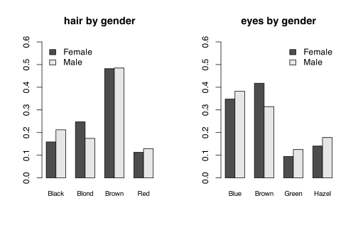
11.21- Eye and hair colour are strongly dependent in this population of 6800: \(\chi^2 = 1073.5\) (6 df, \(p\) essentially 0), \(\Phi^2 = 0.158\), \(V^2 = 0.079\), \(C = 0.369\); the contributions show that blue eyes go with blond hair and brown eyes with brown or black hair, while red hair is distributed independently of eye colour.
eh <- matrix(c(1768, 807, 189, 47,
946, 1387, 746, 53,
115, 438, 288, 16), nrow = 3, byrow = TRUE,
dimnames = list(Eyes = c("Blue", "Grey/green", "Brown"),
Hair = c("Blond", "Brown", "Black", "Red")))
round(chisq.test(eh)$expected, 1)
round(chisq.test(eh)$residuals^2, 1)
assoc(eh)
round(prop.table(eh, 1), 3)
Hair
Eyes Blond Brown Black Red
Blue 1169.5 1088.0 505.6 48.0
Grey/green 1303.0 1212.3 563.3 53.4
Brown 356.5 331.7 154.1 14.6
Hair
Eyes Blond Brown Black Red
Blue 306.3 72.6 198.2 0.0
Grey/green 97.8 25.2 59.3 0.0
Brown 163.6 34.1 116.3 0.1
chi2 Phi2 V2 C
1073.5076 0.1579 0.0789 0.3692
Hair
Eyes Blond Brown Black Red
Blue 0.629 0.287 0.067 0.017
Grey/green 0.302 0.443 0.238 0.017
Brown 0.134 0.511 0.336 0.019
The row profiles confirm it: 62.9% of blue-eyed people are blond against 13.4% of brown-eyed people, whereas the proportion of red hair is 1.7-1.9% in every eye-colour group.
Worksheet 11.W.B — Descriptive analysis of the data set NUTRIELDERLY
Worksheet 11.W.B — Descriptive data studies — Descriptive analysis of data set NutriElderly
We now propose to solve the following questions on the dataset NutriElderly, in which deliberate errors were introduced.
11.1- Import the data file nutrition_elderly.xls.
11.2- Give the absolute mode of variables situation, chocol and height.
11.3- Choose classes for variable height and give the modal class.
11.4- Calculate the median of variable chocol.
11.5- Give frequency tables of variables chocol and raw_fruit.
11.6- Using only these frequency tables, give the median of these two variables.
11.7- Calculate the quartiles of variable height using the classes defined earlier.
11.8- Draw the cumulative frequency polygon for variable height. On this plot, estimate the quartiles of the distribution.
11.9- Using individual data, calculate the mean of variables height, weight and age.
11.10- Calculate the frequency table of variable tea. Using this table, calculate the mean of this variable.
11.11- Calculate the mean of variable height using the classes defined earlier.
11.12- Calculate the range of variable weight.
11.13- Draw a boxplot of variable weight.
11.14- Using individual data, calculate the standard deviation of variable height.
11.15- Using only its frequency table, calculate the coefficient of variation of variable tea.
11.16- Calculate the total variance, the within-group variance and the between-group variance of variable coffee with the population split into two groups: males and females. Calculate the coefficient \(\eta^2\).
11.1- Download the file and read it with read_excel() from readxl (the book’s gdata::read.xls() was removed in gdata 3.0), check every code against its admissible set, then structure the variables as in Section 11.2.
library(readxl)
tf <- tempfile(fileext = ".xls")
download.file("http://www.biostatisticien.eu/springeR/nutrition_elderly.xls",
tf, mode = "wb", quiet = TRUE)
ne <- as.data.frame(read_excel(tf))
dim(ne)
# Admissible codes (Section 11.2): any value outside them is an error
ok <- list(gender = 1:2, situation = 1:4, fat = 1:8, meat = 0:5, fish = 0:5,
raw_fruit = 0:5, cooked_fruit_veg = 0:5, chocol = 0:5)
sapply(names(ok), function(v) sum(!ne[[v]] %in% ok[[v]]))
sapply(ne[c("tea", "coffee", "height", "weight", "age")], range)
sum(is.na(ne))
# Structuring (Section 11.2)
ne$gender <- factor(ne$gender, levels = 1:2, labels = c("Male", "Female"))
ne$situation <- factor(ne$situation, levels = 1:4,
labels = c("single", "couple", "family", "other"))
ne$fat <- factor(ne$fat, levels = 1:8, labels = c("butter", "margarine",
"peanut", "sunflower", "olive", "Isio4", "rapeseed", "duck"))
mylevels <- c("never", "< 1/week.", "1/week.", "2-3/week.", "4-6/week.", "1/day")
for (v in c("meat", "fish", "raw_fruit", "cooked_fruit_veg", "chocol"))
ne[[v]] <- factor(ne[[v]], levels = 0:5, labels = mylevels, ordered = TRUE)
ne$tea <- as.integer(ne$tea); ne$coffee <- as.integer(ne$coffee)
[1] 226 13
gender situation fat meat
0 0 0 0
fish raw_fruit cooked_fruit_veg chocol
0 0 0 0
tea coffee height weight age
[1,] 0 0 140 38 65
[2,] 10 5 188 96 91
[1] 0
The file has 226 individuals and 13 variables; every code is admissible, there are no missing values and the ranges of the quantitative variables are plausible, so the copy served at the book’s URL (and the local mirror, identical) does not contain the deliberate errors announced by the worksheet; all answers below are computed on this clean file.
11.2- With the idiom of Section 11.4.1.1, the modes are couple for situation, 1/day for chocol and 160 cm for height (22 individuals).
modes <- function(x) { t <- table(x); names(t)[t == max(t)] }
modes(ne$situation); modes(ne$chocol); modes(ne$height)
max(table(ne$height))
[1] "couple"
[1] "1/day"
[1] "160"
[1] 22
11.3- Take the ten classes of width 5 cm from 140 to 190 (the Sturges classes of Section 11.3.3); the modal class is \(]155, 160]\) with 50 individuals.
brk <- seq(140, 190, by = 5)
tab.h <- table(cut(ne$height, brk, include.lowest = TRUE))
tab.h
names(which.max(tab.h))
[140,145] (145,150] (150,155] (155,160] (160,165] (165,170] (170,175] (175,180]
1 7 37 50 46 31 27 17
(180,185] (185,190]
4 6
[1] "(155,160]"
11.4- chocol is ordinal, so use the book’s my.median() (Section 11.4.1.2): with \(N = 226\) the observations of rank 113 and 114 are both 1/week., which is the median.
my.median <- function(x) {
if (is.numeric(x)) return(median(x))
if (is.ordered(x)) {
N <- length(x)
if (N %% 2) return(sort(x)[(N + 1) / 2]) else {
inf <- sort(x)[N / 2]; sup <- sort(x)[N / 2 + 1]
if (inf == sup) return(inf) else return(c(inf, sup))
}}
stop("Cannot calculate the median for this type of data.")
}
my.median(ne$chocol)
[1] 1/week.
Levels: never < < 1/week. < 1/week. < 2-3/week. < 4-6/week. < 1/day
11.5- Divide the table of counts by \(N\) (Section 11.3.2).
tf.chocol <- table(ne$chocol) / nrow(ne)
tf.fruit <- table(ne$raw_fruit) / nrow(ne)
round(rbind(chocol = tf.chocol, raw_fruit = tf.fruit), 3)
never < 1/week. 1/week. 2-3/week. 4-6/week. 1/day
chocol 0.221 0.274 0.071 0.097 0.049 0.288
raw_fruit 0.009 0.035 0.035 0.062 0.097 0.761
Three quarters of the elderly eat raw fruit every day, while chocolate consumption is split between “never/rarely” and “every day”.
11.6- The median of an ordinal variable is the first level whose cumulative frequency reaches 50 %: 1/week. for chocol (cumulative frequency jumps from 0.496 to 0.566) and 1/day for raw_fruit (from 0.239 to 1), in agreement with 11.4.
med.ord.freq <- function(f) names(f)[which(cumsum(f) >= 0.5)[1]]
round(rbind(chocol = cumsum(tf.chocol), raw_fruit = cumsum(tf.fruit)), 3)
c(chocol = med.ord.freq(tf.chocol), raw_fruit = med.ord.freq(tf.fruit))
never < 1/week. 1/week. 2-3/week. 4-6/week. 1/day
chocol 0.221 0.496 0.566 0.664 0.712 1
raw_fruit 0.009 0.044 0.080 0.142 0.239 1
chocol raw_fruit
"1/week." "1/day"
11.7- Interpolate linearly on the cumulative frequency polygon of the classes (the formula of Section 11.4.1.2, applied to 25 %, 50 % and 75 %), which approx() does in one call: \(q_1 \approx 156.2\), \(m_e \approx 162.0\) and \(q_3 \approx 169.6\) cm. The book’s median.for.freq() cannot be used as printed, since is.numeric(names(x)) is always FALSE and it returns NA (as its own printed output shows).
cfp <- c(0, cumsum(tab.h)) / sum(tab.h)
q.h <- approx(cfp, brk, xout = c(0.25, 0.5, 0.75), ties = "ordered")$y
names(q.h) <- c("q1", "me", "q3"); round(q.h, 2)
q1 me q3
156.15 161.96 169.60
11.8- Plot the points \((e_k, \mathrm{CFP}(e_k))\) joined by segments and read the abscissae where the polygon crosses the levels 0.25, 0.5 and 0.75: about 156, 162 and 170 cm, the values of 11.7.
plot(brk, cfp, type = "b", pch = 19, xlab = "height (cm)",
ylab = "cumulative frequency", main = "Cumulative frequency polygon of height")
segments(140, c(0.25, 0.5, 0.75), q.h, c(0.25, 0.5, 0.75), lty = 2, col = "red")
segments(q.h, 0, q.h, c(0.25, 0.5, 0.75), lty = 2, col = "red")
text(q.h, 0.05, round(q.h, 1), pos = 4, col = "red", cex = 0.8)
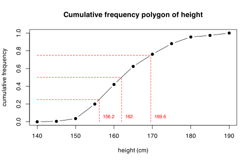
11.9- The mean height is 163.96 cm, the mean weight 66.48 kg and the mean age 74.48 years.
sapply(ne[c("height", "weight", "age")], mean)
height weight age
163.96018 66.48230 74.47788
11.10- With frequencies \(f_k\) of the values \(x_k\), the mean is \(\bar{x} = \sum_k f_k x_k = 0.712\) cup of tea per day, the same as mean(ne$tea) since no information is lost for a discrete variable.
tf.tea <- table(ne$tea) / nrow(ne)
round(tf.tea, 3)
x.tea <- as.numeric(names(tf.tea))
sum(x.tea * tf.tea)
0 1 2 3 4 5 6 9 10
0.721 0.058 0.128 0.035 0.040 0.004 0.004 0.004 0.004
[1] 0.7123894
Almost three quarters (72.1 %) of the elderly never drink tea.
11.11- Replace each observation by the midpoint of its class: the grouped mean is 163.23 cm, close to the exact 163.96 cm of 11.9.
mid <- (brk[-1] + brk[-length(brk)]) / 2
sum(mid * tab.h) / sum(tab.h)
[1] 163.2301
11.12- The range of weight is \(96 - 38 = 58\) kg.
range(ne$weight); diff(range(ne$weight))
[1] 38 96
[1] 58
11.13- Use boxplot() (Section 11.6.3.5); the five numbers drawn are 38, 57, 66, 75 and 96 kg, and there is no outlier.
boxplot(ne$weight, col = "orange", horizontal = TRUE,
xlab = "weight (kg)", main = "Boxplot for variable weight")
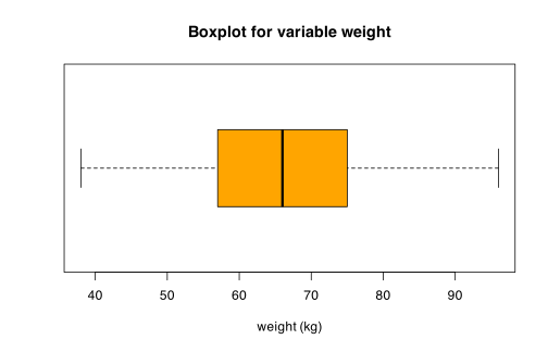
boxplot.stats(ne$weight)$stats; boxplot.stats(ne$weight)$out
[1] 38 57 66 75 96
numeric(0)
The distribution of weight is roughly symmetric around the median of 66 kg, with whiskers reaching the extreme values.
11.14- With the population standard deviation of Section 11.4.2, \(\sigma = 8.98\) cm (sd(), which divides by \(N-1\), gives 9.00 cm).
var.pop <- function(x) var(x) * (length(x) - 1) / length(x)
sd.pop <- function(x) sqrt(var.pop(x))
sd.pop(ne$height); sd(ne$height)
[1] 8.983427
[1] 9.003368
11.15- From the frequency table of 11.10, \(\mu = \sum_k f_k x_k\), \(\sigma = \sqrt{\sum_k f_k (x_k - \mu)^2}\) and \(cv = \sigma / \mu = 2.03\).
mu <- sum(x.tea * tf.tea)
sigma <- sqrt(sum(tf.tea * (x.tea - mu)^2))
c(mean = mu, sd = sigma, cv = sigma / mu)
mean sd cv
0.7123894 1.4456301 2.0292696
The standard deviation is twice the mean: tea consumption is very heterogeneous, most people drinking none and a few drinking up to 10 cups a day.
11.16- With \(K = 2\) groups of sizes \(n_k\), means \(\bar{y}_k\) and (population) variances \(\sigma_k^2\),
\begin{equation*} \begin{aligned} \sigma^2_{\text{within}} &= \frac{1}{N} \sum_{k} n_k \sigma_k^2, \qquad \sigma^2_{\text{between}} = \frac{1}{N} \sum_{k} n_k (\bar{y}_k - \bar{y})^2,\\ \sigma^2_{\text{total}} &= \sigma^2_{\text{within}} + \sigma^2_{\text{between}}, \qquad \eta^2 = \sigma^2_{\text{between}} / \sigma^2_{\text{total}}. \end{aligned} \end{equation*}
y <- ne$coffee; g <- ne$gender
n.k <- tapply(y, g, length); m.k <- tapply(y, g, mean); v.k <- tapply(y, g, var.pop)
rbind(n = n.k, mean = m.k, var = v.k)
v.tot <- var.pop(y)
v.within <- sum(n.k * v.k) / length(y)
v.between <- sum(n.k * (m.k - mean(y))^2) / length(y)
c(total = v.tot, within = v.within, between = v.between,
sum = v.within + v.between, eta2 = v.between / v.tot)
summary(lm(y ~ g))$r.squared
Male Female
n 85.000000 141.000000
mean 1.870588 1.468085
var 1.595017 1.483024
total within between sum eta2
1.56316078 1.52514537 0.03801541 1.56316078 0.02431958
[1] 0.02431958
The total variance 1.563 splits into 1.525 within and 0.038 between the sexes, so \(\eta^2_{\text{coffee}|\text{gender}} = 0.024\) (the same value as the \(R^2\) of Section 11.5.4.1): although men drink slightly more coffee (1.87 vs 1.47 cups a day), gender explains only 2.4 % of the variation in coffee consumption. The authors’ companion solution applies its \(\eta^2\) function to tea rather than coffee; the statement asks for coffee, which is what is computed here.
Worksheet 11.W.C — Descriptive analysis of data sets
Worksheet 11.W.C — Descriptive analysis of data sets — Birth weight and myocardial infarction
The two data sets are described in Appendix B: B- is the weight-at-birth study (Section B.2, 189 mothers seen at the Baystate medical centre in 1986; file Birth_weight.txt) and I is the myocardial infarction study (Section B.5, 149 women who had an infarction and 300 controls; file Infarction.xls).
11.1- Perform a descriptive statistical analysis of data set B-.
11.2- Perform a descriptive statistical analysis of data set I.
11.1- Birth weight averages 2945 g (sd 729 g, 31.2% of babies under 2500 g). The descriptors most strongly linked to it are uterine irritability (\(\eta^2=0.080\)), race (\(0.051\)) and smoking (\(0.036\)), and each explains only a few percent of its variance. Import this irregular text file as in question 4.4 of Worksheet 4.W.C, then recode the qualitative variables as factors (Section 11.2):
url <- "http://www.biostatisticien.eu/springeR/Birth_weight.txt"
bw <- read.table(url, row.names = 1, skip = 1, header = FALSE, sep = ";",
nrows = 189, blank.lines.skip = TRUE)
colnames(bw) <- as.matrix(read.table(url, nrows = 1, row.names = 1))
bw$RACE <- factor(bw$RACE, labels = c("White", "Black", "Other"))
for (v in c("SMOKE", "HT", "UI", "LOW"))
bw[[v]] <- factor(bw[[v]], levels = 0:1, labels = c("No", "Yes"))
dim(bw)
[1] 189 10
Univariate summaries of the quantitative variables (Section 11.4; skewness() and kurtosis() come from e1071):
library(e1071)
quanti <- bw[, c("AGE", "LWT", "PTL", "FVT", "BWT")]
round(t(sapply(quanti, function(x) c(mean = mean(x), sd = sd(x),
quantile(x), IQR = IQR(x), cv = sd(x) / mean(x),
skew = skewness(x), kurt = kurtosis(x)))), 2)
table(bw$PTL); table(bw$FVT)
mean sd 0% 25% 50% 75% 100% IQR cv skew kurt
AGE 23.24 5.30 14 19 23 26 45 7 0.23 0.71 0.53
LWT 129.81 30.58 80 110 121 140 250 30 0.24 1.38 2.25
PTL 0.20 0.49 0 0 0 0 3 0 2.52 2.76 8.17
FVT 0.79 1.06 0 0 0 1 6 1 1.33 1.56 3.00
BWT 2944.66 729.02 709 2414 2977 3475 4990 1061 0.25 -0.21 -0.14
0 1 2 3
159 24 5 1
0 1 2 3 4 6
100 47 30 7 4 1
The mothers are young (median 23 years) and the mother’s weight is right-skewed (skewness 1.38). PTL and FVT are small counts heaped at 0: 84% of mothers had no previous premature birth and 53% had no first-trimester visit. BWT itself is nearly symmetric (skewness \(-0.21\), excess kurtosis \(-0.14\)).
Frequency tables (in %) of the qualitative variables (Section 11.3):
round(100 * prop.table(table(bw$RACE)), 1)
sapply(bw[, c("SMOKE", "HT", "UI", "LOW")],
function(f) round(100 * prop.table(table(f)), 1))
White Black Other
50.8 13.8 35.4
SMOKE HT UI LOW
No 60.8 93.7 85.2 68.8
Yes 39.2 6.3 14.8 31.2
Half of the mothers are white, 39.2% smoked during pregnancy, and hypertension (6.3%) and uterine irritability (14.8%) are uncommon.
Measures of association with the birth weight (Section 11.5). For each factor, the output gives the conditional means and the correlation ratio \(\eta^2_{\text{BWT}|X}\) computed with the book’s eta2(), followed by the linear correlations with the quantitative variables:
eta2 <- function(x, gpe) {
means <- tapply(x, gpe, mean); counts <- tapply(x, gpe, length)
sum(counts * (means - mean(x))^2) / (var(x) * (length(x) - 1))
}
lapply(bw[, c("SMOKE", "RACE", "HT", "UI")], function(g)
round(c(tapply(bw$BWT, g, mean), eta2 = eta2(bw$BWT, g)), 3))
round(cor(quanti)["BWT", ], 2)
$SMOKE
No Yes eta2
3054.957 2773.243 0.036
$RACE
White Black Other eta2
3103.740 2719.692 2804.015 0.051
$HT
No Yes eta2
2972.311 2536.750 0.021
$UI
No Yes eta2
3030.609 2450.429 0.080
AGE LWT PTL FVT BWT
0.09 0.19 -0.15 0.06 1.00
Babies of smokers are 282 g lighter on average. Babies of white mothers are about 300 to 385 g heavier than those of the other two groups, and hypertension and uterine irritability each lower the mean by 435 to 580 g. All the correlation ratios and correlations are small, the largest correlation being \(r=0.19\) with the mother’s weight. The binary outcome LOW gives the same picture:
tab <- table(bw$SMOKE, bw$LOW, dnn = c("SMOKE", "LOW"))
round(100 * prop.table(tab, 1), 1)
chi <- chisq.test(tab, correct = FALSE)
c(chi2 = unname(chi$statistic), V2 = unname(chi$statistic) / sum(tab),
p = chi$p.value)
LOW
SMOKE No Yes
No 74.8 25.2
Yes 59.5 40.5
chi2 V2 p
4.92370543 0.02605135 0.02649064
40.5% of smokers had a low-weight baby, compared with 25.2% of non-smokers. The link is weak (\(V^2 = \Phi^2 = 0.026\)) but it is significant at the 5% level (\(\chi^2=4.92\), \(p=0.026\)). Graphical summary (Section 11.6):
par(mfrow = c(2, 2), mar = c(4, 4, 2, 1))
hist(bw$BWT, main = "Birth weight", xlab = "BWT (g)", col = "grey")
abline(v = 2500, lty = 2)
boxplot(BWT ~ SMOKE, data = bw, main = "BWT by smoking", col = "grey")
boxplot(BWT ~ RACE, data = bw, main = "BWT by race", col = "grey")
plot(BWT ~ LWT, data = bw, main = "BWT vs mother's weight", pch = 20)
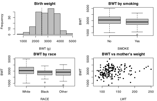
11.2- Infarction cases differ from controls mainly in their exposures. 56% of oral-contraceptive users are cases, compared with 14.9% of never-users (\(V^2=0.189\)), and tobacco (current or former) shows a similar gap (\(V^2=0.132\)). Age and height hardly differ between cases and controls. The book imports the file with read.xls(), which the current gdata no longer provides, so the equivalent readxl call is used here, again with “.” declared as the missing-value code:
library(readxl)
url <- "http://www.biostatisticien.eu/springeR/Infarction.xls"
tf <- tempfile(fileext = ".xls")
download.file(url, tf, mode = "wb", quiet = TRUE)
inf <- as.data.frame(read_excel(tf, na = "."))
inf$INFARCT <- factor(inf$INFARCT, labels = c("Control", "Case"))
inf$TOBACCO <- factor(inf$TOBACCO, labels = c("No", "Smoker", "Former"))
for (v in c("CO", "ATCD", "HTA"))
inf[[v]] <- factor(inf[[v]], levels = 0:1, labels = c("No", "Yes"))
colSums(is.na(inf))[colSums(is.na(inf)) > 0]
WEIGHT BMI ATCD
12 12 7
Twelve weights (and hence twelve BMIs) and seven family histories are missing. Each summary below therefore uses the available values only. Univariate summaries of the quantitative variables (Section 11.4):
library(e1071)
round(t(sapply(inf[, c("AGE", "WEIGHT", "HEIGHT", "BMI")], function(x) {
x <- na.omit(x)
c(n = length(x), mean = mean(x), sd = sd(x), quantile(x),
cv = sd(x) / mean(x), skew = skewness(x), kurt = kurtosis(x))})), 2)
n mean sd 0% 25% 50% 75% 100% cv skew kurt
AGE 449 45.62 16.17 15.00 33.00 44.00 56.00 100.00 0.35 0.50 0.02
WEIGHT 437 66.07 17.96 33.00 51.00 64.00 79.00 128.00 0.27 0.65 0.00
HEIGHT 449 165.16 8.11 138.00 160.00 166.00 171.00 184.00 0.05 -0.33 -0.06
BMI 437 24.38 7.13 11.36 18.67 23.18 29.17 47.78 0.29 0.70 -0.03
The women are aged 15 to 100 (median 44). Weight and BMI are moderately right-skewed, while height is almost symmetric and has little spread (cv 0.05). Frequency tables (in %) of the qualitative variables (Section 11.3), where the cases make up 149/449 = 33.2% of the sample by design:
round(100 * prop.table(table(inf$TOBACCO)), 1)
sapply(inf[, c("CO", "ATCD", "HTA")],
function(f) round(100 * prop.table(table(f)), 1))
No Smoker Former
47.9 30.1 22.0
CO ATCD HTA
No 55.5 88 64.6
Yes 44.5 12 35.4
The next block compares cases with controls (Section 11.5). For the quantitative variables it gives the conditional means and the correlation ratio \(\eta^2\), using the book’s eta2():
eta2 <- function(x, gpe) {
means <- tapply(x, gpe, mean); counts <- tapply(x, gpe, length)
sum(counts * (means - mean(x))^2) / (var(x) * (length(x) - 1))
}
round(t(sapply(c("AGE", "WEIGHT", "HEIGHT", "BMI"), function(v) {
ok <- !is.na(inf[[v]])
c(tapply(inf[[v]][ok], inf$INFARCT[ok], mean),
eta2 = eta2(inf[[v]][ok], inf$INFARCT[ok]))})), 3)
Control Case eta2
AGE 44.967 46.933 0.003
WEIGHT 63.510 71.214 0.041
HEIGHT 165.353 164.772 0.001
BMI 23.404 26.358 0.038
Cases are on average 7.7 kg heavier than controls (BMI 26.4 against 23.4), yet infarction status still explains only about 4% of the variance of weight. The age and height differences are negligible (\(\eta^2 \le 0.003\)). For the qualitative variables, the next block gives the percentage of cases in each level, Cramér’s \(V^2\) and the \(\chi^2\) p-value:
lapply(inf[, c("CO", "TOBACCO", "ATCD", "HTA")], function(g) {
tab <- table(g, inf$INFARCT)
chi <- chisq.test(tab, correct = FALSE)
round(c(100 * prop.table(tab, 1)[, "Case"],
V2 = unname(chi$statistic) / (sum(tab) * (min(dim(tab)) - 1)),
p = chi$p.value), 4)})
$CO
No Yes V2 p
14.8594 56.0000 0.1886 0.0000
$TOBACCO
No Smoker Former V2 p
15.8140 44.4444 55.5556 0.1321 0.0000
$ATCD
No Yes V2 p
31.8766 41.5094 0.0044 0.1619
$HTA
No Yes V2 p
29.3103 40.2516 0.0123 0.0185
Oral contraceptives and tobacco are the two clearly associated factors (\(p<10^{-4}\)). Hypertension is weakly associated: 40.3% of hypertensive women are cases against 29.3% of the others (\(p=0.019\)). Family history shows no significant link at the 5% level (\(p=0.16\)). Graphical summary (Section 11.6):
par(mfrow = c(1, 3), mar = c(4, 4, 2, 1))
boxplot(AGE ~ INFARCT, data = inf, main = "Age", col = "grey", xlab = "")
boxplot(BMI ~ INFARCT, data = inf, main = "BMI", col = "grey", xlab = "")
barplot(prop.table(table(inf$INFARCT, inf$TOBACCO), 2),
main = "Infarction by tobacco", legend.text = TRUE,
args.legend = list(x = "topleft", cex = 0.8))
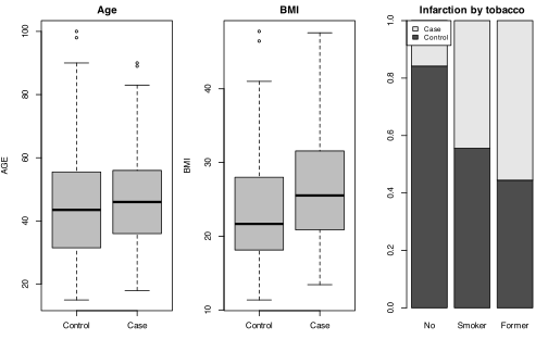
Random variables, distributions and simulations
Exercises 12.1–12.7
Which R function would you use to generate numbers from a \(\mathcal{N}(0,1)\) distribution?
rnorm(), whose defaults mean = 0, sd = 1 are exactly the \(\mathcal{N}(0,1)\) distribution (Table 12.2), so only the sample size is needed (seed 1):
set.seed(1)
rnorm(5)
[1] -0.6264538 0.1836433 -0.8356286 1.5952808 0.3295078
Which R function would you use to generate numbers from a \(\mathcal{N}(2,10)\) distribution?
rnorm() with mean = 2 and sd = sqrt(10): the book writes \(\mathcal{N}(\mu,\sigma^2)\), but R’s argument is the standard deviation \(\sigma\), not the variance (seed 1):
set.seed(1)
rnorm(5, mean = 2, sd = sqrt(10))
[1] 0.01897911 2.58073118 -0.64248969 7.04472084 3.04199507
Which R function would you use to calculate the quantiles of a \(\chi^2\) distribution?
qchisq(p, df), with the degrees of freedom in df; e.g. the 2.5%, 50% and 97.5% quantiles of a \(\chi^2_5\):
qchisq(c(0.025, 0.5, 0.975), df = 5)
[1] 0.8312116 4.3514602 12.8325020
Which R function would you use to calculate the density of a Fisher distribution?
df(x, df1, df2), with the numerator and denominator degrees of freedom in df1 and df2; e.g. for \(\mathcal{F}(3,10)\):
df(c(0.5, 1, 2), df1 = 3, df2 = 10)
[1] 0.6340072 0.4041228 0.1482109
Which R function would you use to calculate the quantiles of a Student distribution?
qt(p, df), with the degrees of freedom in df; e.g. the 2.5% and 97.5% quantiles of a \(\mathcal{T}_{10}\):
qt(c(0.025, 0.975), df = 10)
[1] -2.228139 2.228139
How would you compute the probability that X lays between 3 and 5 given that \(X \sim \mathcal{N}(4,2)\)?
As a difference of the distribution function, \(P(3 \le X \le 5) = F(5) - F(3)\), with pnorm() and sd = sqrt(2) since the second parameter is the variance:
pnorm(5, mean = 4, sd = sqrt(2)) - pnorm(3, mean = 4, sd = sqrt(2))
[1] 0.5204999
So \(P(3 \le X \le 5) \approx 0.5205\); the authors’ companion solution uses mean = 2, a slip for the stated mean of 4.
How would you calculate the quantile of order \(p = 0.95\) of a \(\mathcal{N}(0,1)\)?
qnorm(0.95), since qnorm() defaults to mean = 0, sd = 1:
qnorm(0.95)
[1] 1.644854
Worksheet 12.W.A — Simulations - Study of the distribution f(x) = (3/2) sqrt(x) on [0, 1]
Worksheet 12.W.A — Simulations — Study of the distribution \(f(x) = \frac{3}{2}\sqrt{x}\) on \([0, 1]\)
12.1- Check that \(f(x)\) is a density, using the function integrate().
12.2- Simulate a sample of size 1,000 from the distribution defined by the density \(f(x) = \frac{3}{2}\sqrt{x}\) over \([0, 1]\).
12.3- Calculate the empirical mean and variance.
12.4- Compare with the theoretical values.
12.5- Calculate and compare the theoretical and empirical probabilities of the following classes: \([0, 0.30]\), \(]0.30, 0.50]\), \(]0.50, 0.70]\), \(]0.70, 0.85]\), \(]0.85, 1]\).
12.1- \(f \ge 0\) on \([0,1]\) and its integral is 1, so \(f\) is a density:
f <- function(x) 3/2 * sqrt(x)
integrate(f, lower = 0, upper = 1)
1 with absolute error < 0.00012
12.2- Use the inverse transform method of Section 12.5.2: \(F(x) = x^{3/2}\) on \([0,1]\), so \(F^{-1}(u) = u^{2/3}\) and \(X = U^{2/3}\) with \(U \sim U[0,1]\) has density \(f\).
set.seed(1)
x <- runif(1000)^(2/3)
head(round(x, 4))
[1] 0.4131 0.5174 0.6898 0.9378 0.3439 0.9311
12.3- With set.seed(1), the empirical mean is 0.6003 and the (unbiased, Section 12.4.1) empirical variance is 0.0677:
c(mean = mean(x), var = var(x))
mean var
0.60029442 0.06767857
12.4- The theoretical values are \(E(X) = \int_0^1 \frac{3}{2}x^{3/2}\,dx = \frac{3}{5}\) and \(\mathrm{Var}(X) = \frac{3}{7} - \frac{9}{25} = \frac{12}{175} \approx 0.0686\), computed here with integrate():
mu <- integrate(function(x) x * f(x), 0, 1)$value
sigma2 <- integrate(function(x) x^2 * f(x), 0, 1)$value - mu^2
rbind(theoretical = c(mean = mu, var = sigma2),
empirical = c(mean(x), var(x)))
mean var
theoretical 0.6000000 0.06857143
empirical 0.6002944 0.06767857
The empirical mean and variance agree with the theoretical ones to within about 0.0003 and 0.001, which is the sampling variation expected with \(n = 1000\) (law of large numbers, Section 12.3.1).
12.5- The theoretical probability of \(]a, b]\) is \(F(b) - F(a) = b^{3/2} - a^{3/2}\); the empirical one is the proportion of the sample falling in the class, obtained with cut() and table():
breaks <- c(0, 0.30, 0.50, 0.70, 0.85, 1)
F <- function(q) q^(3/2)
emp <- table(cut(x, breaks, include.lowest = TRUE)) / length(x)
round(rbind(theoretical = diff(F(breaks)), empirical = emp), 4)
[0,0.3] (0.3,0.5] (0.5,0.7] (0.7,0.85] (0.85,1]
theoretical 0.1643 0.1892 0.2321 0.198 0.2163
empirical 0.1610 0.1900 0.2410 0.198 0.2100
Every empirical frequency is within 0.01 of its theoretical probability (largest gap 0.009 on \(]0.50, 0.70]\)), so the simulated sample reproduces the distribution \(f\) well.
Worksheet 12.W.B — Study of the generalized Pareto distribution
Worksheet 12.W.B — Study of the generalized Pareto distribution
Let \(X\) be a random variable following a generalized Pareto distribution \(GP(\mu,\sigma,\xi)\). The density of this distribution is
\begin{equation*} f_X(x) = \frac{1}{\sigma}\left(1 + \frac{\xi(x-\mu)}{\sigma}\right)^{-\frac{1}{\xi}-1} \end{equation*}
with \(x \ge \mu\) if \(\xi \ge 0\) and \(x \le \mu - \sigma/\xi\) if \(\xi < 0\). It is given that
\begin{equation*} \mathbb{E}(X) = \mu + \frac{\sigma}{1-\xi} \quad (\xi < 1) \end{equation*}
and
\begin{equation*} \mathrm{Var}(X) = \frac{\sigma^2}{(1-\xi)^2(1-2\xi)} \quad (\xi < 1/2). \end{equation*}
We can simulate from \(X\) with the following formula:
\begin{equation*} X = \mu + \frac{\sigma(U^{-\xi} - 1)}{\xi} \end{equation*}
where \(U\) is a uniform random variable over \([0,1]\).
12.1- Propose an R code to generate a sample of size \(n\) from a \(GP(\mu,\sigma,\xi)\) distribution. Your source code should use the following variables: n, mu, sigma and xi.
12.2- Simulate a sample of size \(n = 1{,}000\) from the distribution \(GP(0, 1, 1/4)\).
12.3- Calculate the empirical mean and variance.
12.4- Compare with the theoretical values.
12.5- Repeat questions 2 to 3 with \(n = 10{,}000\).
12.6- Plot in red the density histogram of your sample. Take 500 equidistant classes and limit the display of the histogram to the interval \([0, 10]\) on the x-axis.
12.7- Overlay the density plot of the \(GP(0, 1, 1/4)\) distribution (in blue). Note that the plot is close to the histogram.
12.1- Apply the given inversion formula to runif() draws, vectorised over the \(n\) uniforms:
rGP <- function(n, mu, sigma, xi) mu + sigma * (runif(n)^(-xi) - 1) / xi
12.2- With set.seed(1):
set.seed(1)
n <- 1000; mu <- 0; sigma <- 1; xi <- 1/4
x <- rGP(n, mu, sigma, xi)
head(round(x, 4))
[1] 1.5724 1.1214 0.5978 0.0975 1.9689 0.1086
12.3- The empirical mean is 1.294 and the empirical variance 2.749 (seed 1):
c(mean = mean(x), var = var(x))
mean var
1.293959 2.748602
12.4- The theoretical values are \(\mathbb{E}(X) = 1/(3/4) = 4/3 \approx 1.333\) and \(\mathrm{Var}(X) = 1/\big((9/16)(1/2)\big) = 32/9 \approx 3.556\):
c(mean = mu + sigma/(1 - xi), var = sigma^2/((1 - xi)^2 * (1 - 2*xi)))
mean var
1.333333 3.555556
The empirical mean is within 3% of \(4/3\), but the empirical variance undershoots \(32/9\) by about 23%: with \(\xi = 1/4\) the fourth moment of \(X\) is infinite, so the sample variance converges slowly and is driven by rare large values.
12.5- With \(n = 10{,}000\) (seed 1) the mean is 1.348 and the variance 3.573, both now close to \(4/3\) and \(32/9\):
set.seed(1)
n <- 10000
x <- rGP(n, mu, sigma, xi)
c(mean = mean(x), var = var(x))
mean var
1.348422 3.573066
12.6- and 12.7- hist(freq = FALSE) draws the density histogram and curve(add = TRUE) overlays the density \(f_X(x) = (1 + x/4)^{-5}\):
dGP <- function(x, mu, sigma, xi) (1 + xi * (x - mu) / sigma)^(-1/xi - 1) / sigma
hist(x, breaks = 500, freq = FALSE, col = "red", border = "red", xlim = c(0, 10),
main = "GP(0, 1, 1/4): n = 10,000", xlab = "x")
curve(dGP(x, mu, sigma, xi), from = 0, to = 10, col = "blue", lwd = 2, add = TRUE)
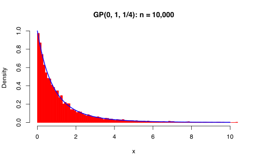
The blue density follows the red histogram closely across \([0, 10]\), confirming that the inversion formula generates \(GP(0, 1, 1/4)\) draws; breaks = 500 splits the whole sample range (maximum 35.4 here) into classes, of which only those in \([0, 10]\) are displayed.
Worksheet 12.W.C — Uniform distribution on a square
Worksheet 12.W.C — Uniform distribution on a square — Uniform distribution on a square
12.1- Simulate 1,000 observations from \((X_1, X_2)\) which follow the uniform distribution over the square \([0,1] \times [0,1]\).
12.2- Get an approximation of the probability that the distance between \((X_1, X_2)\) and the nearest edge is less than 0.25.
12.3- Same question for the distance to the nearest vertex.
12.4- Try to identify the theoretical distribution of the variable distance to the nearest edge: expected value, variance, density.
12.1- Fill a two-column matrix with runif(2*n) (seed 1), since \(X_1\) and \(X_2\) are independent \(U[0,1]\):
set.seed(1)
n <- 1000
X <- matrix(runif(2 * n), ncol = 2, dimnames = list(NULL, c("X1", "X2")))
head(X, 3)
X1 X2
[1,] 0.2655087 0.5308088
[2,] 0.3721239 0.6848609
[3,] 0.5728534 0.3832834
12.2- The estimate is 0.767. The distance to the nearest edge is \(D = \min(X_1, 1-X_1, X_2, 1-X_2)\), and the probability is estimated by the proportion of simulated points with \(D < 0.25\):
d.edge <- apply(cbind(X, 1 - X), 1, min)
mean(d.edge < 0.25)
[1] 0.767
This is close to the exact value \(1 - (1 - 2 \times 0.25)^2 = 0.75\), the area of the square minus the central square of side \(0.5\) (see 12.4).
12.3- The estimate is 0.205. Take the minimum of the Euclidean distances to the four vertices:
V <- cbind(c(0, 1, 0, 1), c(0, 0, 1, 1))
d.vert <- apply(X, 1, function(p) min(sqrt((p[1] - V[, 1])^2 + (p[2] - V[, 2])^2)))
mean(d.vert < 0.25)
pi / 16
[1] 0.205
[1] 0.1963495
The exact probability is the total area of the four quarter-discs of radius \(0.25\) at the corners, \(\pi (0.25)^2 = \pi/16 \approx 0.196\), which agrees with the simulation.
12.4- \(D\) has density \(f_D(d) = 4(1-2d)\) on \([0, 1/2]\), with \(\mathbb{E}(D) = 1/6\) and \(\mathrm{Var}(D) = 1/72\). Indeed \(D > d\) exactly when the point lies in the central square \([d, 1-d]^2\), so
\begin{equation*} \begin{aligned} P(D > d) &= (1-2d)^2, \qquad F_D(d) = 1 - (1-2d)^2, \qquad f_D(d) = 4(1-2d),\\ \mathbb{E}(D) &= \int_0^{1/2} (1-2d)^2 \, dd = \frac{1}{6}, \qquad \mathbb{E}(D^2) = \int_0^{1/2} 4d^2(1-2d) \, dd = \frac{1}{24},\\ \mathrm{Var}(D) &= \frac{1}{24} - \frac{1}{36} = \frac{1}{72} \approx 0.0139 . \end{aligned} \end{equation*}
The simulated sample confirms this:
c(mean = mean(d.edge), var = var(d.edge))
c(mean = 1/6, var = 1/72)
integrate(function(d) 4 * (1 - 2 * d), 0, 0.5)$value
ks.test(d.edge, function(q) 1 - (1 - 2 * pmin(pmax(q, 0), 0.5))^2)
mean var
0.16175485 0.01360786
mean var
0.16666667 0.01388889
[1] 1
Asymptotic one-sample Kolmogorov-Smirnov test
data: d.edge
D = 0.033624, p-value = 0.2082
alternative hypothesis: two-sided
The empirical mean and variance are close to \(1/6\) and \(1/72\), and the Kolmogorov-Smirnov test (p-value 0.21) does not reject the proposed distribution. Its density fits the histogram well:
hist(d.edge, breaks = 20, freq = FALSE, col = "grey",
main = "Distance to the nearest edge", xlab = "d")
curve(4 * (1 - 2 * x), 0, 0.5, add = TRUE, col = "blue", lwd = 2)
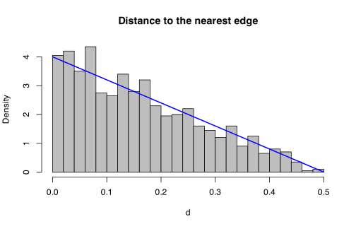
Worksheet 12.W.D — Towards modelling
Worksheet 12.W.D — Towards modelling — Towards modelling
A statistician believes that the world around us and the phenomena that occur are a large entanglement of random events, which can be modelled in a simplified way by random variables.
12.1- Start with the simple, and classical, example, of a coin toss. The outcome of this experiment is the observation of HEAD or TAIL at each toss. This can be modelled by a random variable \(X\) with distribution a Bernoulli with parameter \(1/2\). This experiment can be reproduced with a computer. Create a function X which simulates a coin toss. You can toss your virtual coins a few times.
12.2- We can also propose a modelling of the throw of a die. The outcome of this experiment is the observation of the number on the upper side of the die at each throw. If the die is not weighted, this can be modelled by a random variable \(X\) with distribution a discrete uniform over \(\{1, 2, 3, 4, 5, 6\}\). This experiment can be reproduced with a computer. Create a function throw.die() using the function sample(). You can throw your virtual die a few times.
12.3- To simulate the game of Yahtzee, we shall create a function yahtzee() which throws five virtual dice. Create this function using the parameters size and replace of the function sample().
12.4- Estimate the probability of getting a yahtzee, i.e. five identical dice in one throw (hint: use the functions apply(), replicate() and unique()). You should get a value close to \(\frac{1}{6^4}\).
12.1- Draw a \(\mathcal{B}(1/2)\) value with rbinom(1, 1, 1/2) (Table 12.1) and map \(0/1\) to TAIL/HEAD; replicate() tosses the coin repeatedly (seed 1).
set.seed(1)
X <- function() c("TAIL", "HEAD")[rbinom(1, size = 1, prob = 1/2) + 1]
replicate(8, X())
[1] "TAIL" "TAIL" "HEAD" "HEAD" "TAIL" "HEAD" "HEAD" "HEAD"
12.2- sample(1:6, 1) draws one value uniformly from \(\{1,\dots,6\}\), which is exactly the discrete uniform model; ten throws with seed 1:
set.seed(1)
throw.die <- function() sample(1:6, 1)
replicate(10, throw.die())
[1] 1 4 1 2 5 3 6 2 3 3
12.3- Five independent dice means drawing size = 5 values with replacement (replace = TRUE), otherwise the five faces would be forced to differ; two throws with seed 1:
set.seed(1)
yahtzee <- function() sample(1:6, size = 5, replace = TRUE)
yahtzee()
yahtzee()
[1] 1 4 1 2 5
[1] 3 6 2 3 3
12.4- The estimated probability is \(\hat p = 0.00070\) from \(10^5\) simulated throws (seed 1), close to the exact \(1/6^4 = 6/6^5 \approx 0.000772\). replicate() stores each throw as a column of a \(5 \times n\) matrix, and apply() flags the columns with a single unique() value:
set.seed(1)
n <- 100000
throws <- replicate(n, yahtzee())
p.hat <- mean(apply(throws, 2, function(d) length(unique(d)) == 1))
c(estimate = p.hat, exact = 1/6^4)
round(p.hat + c(-1, 1) * 1.96 * sqrt(p.hat * (1 - p.hat) / n), 6)
estimate exact
0.0007000000 0.0007716049
[1] 0.000536 0.000864
The exact value lies inside the approximate 95% confidence interval \([0.000536, 0.000864]\), so the simulation agrees with \(1/6^4\) up to Monte Carlo error.
Worksheet 12.W.E — Box-Muller theorem
Worksheet 12.W.E — Box-Muller theorem — Box-Muller theorem
Let \(U_1\) and \(U_2\) be two independent random variables uniform over the interval \([0,1]\). The variables
\begin{equation*} \begin{aligned} Z_1 &= \sqrt{-2\log(U_1)}\,\cos(2\pi U_2)\\ Z_2 &= \sqrt{-2\log(U_1)}\,\sin(2\pi U_2) \end{aligned} \end{equation*}
are then two independent standard normal random variables.
12.1- Generate \(n = 1{,}000\) pairs of observations \((z_1,z_2)_1,\ldots,(z_1,z_2)_n\) using this algorithm.
12.2- Use the function kde2d() from package MASS to estimate the bivariate density of these data.
12.3- Use the functions spheres3d() and surface3d() from the package rgl to plot these observations and the surface of the estimated bivariate density of these data. Also plot the surface of the density of a bivariate standard normal distribution. Note that you get a bell plot, typical of the bivariate normal.
12.1- Two vectors of runif() draws pushed through the transformation give the 1,000 pairs (seed 1):
set.seed(1)
n <- 1000
u1 <- runif(n); u2 <- runif(n)
z1 <- sqrt(-2 * log(u1)) * cos(2 * pi * u2)
z2 <- sqrt(-2 * log(u1)) * sin(2 * pi * u2)
z <- cbind(z1, z2)
head(round(z, 4), 3)
round(c(mean(z1), mean(z2), sd(z1), sd(z2), cor(z1, z2)), 3)
z1 z2
[1,] -1.5981 -0.3133
[2,] -0.5595 -1.2899
[3,] -0.7842 0.7066
[1] 0.043 0.003 0.971 1.016 -0.016
Means near 0, standard deviations near 1 and a correlation near 0 are what two independent \(N(0,1)\) samples should show.
12.2- kde2d() returns a list with the grid x, y and the matrix z of estimated density values; here on a \(50\times 50\) grid over \([-3.5,3.5]^2\), compared with the exact density \(\phi(x)\phi(y)\):
library(MASS)
est <- kde2d(z1, z2, n = 50, lims = c(-3.5, 3.5, -3.5, 3.5))
str(est, give.attr = FALSE)
round(max(est$z), 4); round(1 / (2 * pi), 4)
theo <- outer(est$x, est$y, function(x, y) dnorm(x) * dnorm(y))
round(max(abs(est$z - theo)), 4)
List of 3
$ x: num [1:50] -3.5 -3.36 -3.21 -3.07 -2.93 ...
$ y: num [1:50] -3.5 -3.36 -3.21 -3.07 -2.93 ...
$ z: num [1:50, 1:50] 1.51e-19 8.44e-18 3.61e-16 1.17e-14 2.91e-13 ...
[1] 0.1668
[1] 0.1592
[1] 0.0333
The estimated peak (0.167) is close to the theoretical maximum \(1/(2\pi)\approx 0.159\), and the estimate never departs from \(\phi(x)\phi(y)\) by more than 0.033 on the grid.
12.3- With rgl the requested plots are drawn by
library(rgl)
open3d()
spheres3d(z1, z2, 0, radius = 0.05, color = "red")
surface3d(est$x, est$y, 10 * est$z, color = "lightblue", alpha = 0.6)
open3d()
surface3d(est$x, est$y, 10 * theo, color = "pink")
(the factor 10 stretches the vertical axis so the bell is visible next to the points); since rgl cannot render headless, the static equivalent below uses persp(), with the observations projected onto the base plane by trans3d():
par(mfrow = c(1, 2), mar = c(1, 1, 2, 1))
pm <- persp(est$x, est$y, est$z, theta = 30, phi = 25, col = "lightblue",
border = "grey40", xlab = "z1", ylab = "z2", zlab = "density",
main = "kde2d() estimate + data", zlim = c(0, 0.18))
points(trans3d(z1, z2, 0, pm), pch = 16, cex = 0.3, col = "red")
persp(est$x, est$y, theo, theta = 30, phi = 25, col = "lightpink",
border = "grey40", xlab = "z1", ylab = "z2", zlab = "density",
main = "N(0, I2) density", zlim = c(0, 0.18))
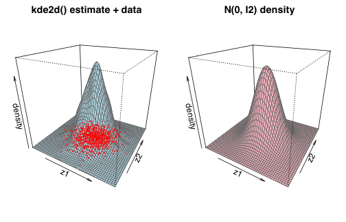
Both surfaces are the same circularly symmetric bell centred at \((0,0)\), confirming that the Box-Muller pairs behave as a bivariate standard normal sample.
Confidence intervals and hypothesis testing
Exercises 13.1–13.7
Which function would you use to get the quantiles of a binomial distribution?
qbinom(p, size, prob), the “q” member of the binom family, returns the smallest integer \(x\) with \(P(X\le x)\ge p\); for \(X\sim\mathcal{B}(20,0.3)\):
qbinom(c(0.025, 0.5, 0.975), size = 20, prob = 0.3)
[1] 2 6 10
What is the use of the function pnorm()?
pnorm(q, mean = 0, sd = 1) evaluates the cumulative distribution function of the normal distribution, \(P(X\le q)\) for \(X\sim N(\mu,\sigma^2)\) (with lower.tail = FALSE it gives \(P(X>q)\), used for p-values):
pnorm(1.96)
pnorm(180, mean = 170, sd = 10)
[1] 0.9750021
[1] 0.8413447
Give the R instruction to get a confidence interval for the mean using a sample of size 50.
t.test(x, conf.level = 0.95)$conf.int (Section 13.2.1); with \(n=50>30\) the Student interval is valid even without normality. On a simulated sample (set.seed(1)):
set.seed(1)
x <- rnorm(50, mean = 10, sd = 2)
t.test(x, conf.level = 0.95)$conf.int
[1] 9.728337 10.673456
attr(,"conf.level")
[1] 0.95
The interval \([9.73,\,10.67]\) covers the true mean 10.
Explain the difference between the functions prop.test() and binom.test().
prop.test() uses the normal (large-sample) approximation to the binomial, so it needs \(np\ge5\) and \(n(1-p)\ge5\), and it can also compare two or more proportions; binom.test() is the exact test/interval (Clopper-Pearson) based on the binomial distribution itself, valid for any \(n\) but for a single proportion only (Sections 13.2.2 and 13.3.1.3). On the book’s 141 successes out of 226:
prop.test(141, 226)$conf.int
binom.test(141, 226)$conf.int
[1] 0.5569177 0.6865847
attr(,"conf.level")
[1] 0.95
[1] 0.5572321 0.6872590
attr(,"conf.level")
[1] 0.95
With \(n=226\) the approximate and exact intervals agree to two decimals.
Name two functions which compare two cumulative distribution functions using two samples.
ks.test(x, y) (two-sample Kolmogorov-Smirnov, \(H_0: F_X=F_Y\) via \(\sup_x|\hat F_1(x)-\hat F_2(x)|\)) and wilcox.test(x, y) (Mann-Whitney, \(H_0: F_X=F_Y\) against a shift), Table 13.4. On two simulated samples (set.seed(1)) differing by a shift of 1:
set.seed(1)
x <- rnorm(30); y <- rnorm(30, mean = 1)
ks.test(x, y)$p.value
wilcox.test(x, y)$p.value
[1] 0.0008995777
[1] 2.410166e-05
Both tests reject equality of the two distributions at the 5 % level.
Which function is used to test whether a sample follows a normal distribution?
shapiro.test(x), the Shapiro-Wilk test of \(H_0\): “the sample comes from a normal distribution” (Section 13.3.3.1; package nortest adds lillie.test(), ad.test(), …). On an exponential sample (set.seed(1)):
set.seed(1)
shapiro.test(rexp(40))
Shapiro-Wilk normality test
data: rexp(40)
W = 0.7696, p-value = 1.669e-06
The p-value \(1.7\times10^{-6}\) rejects normality, as it should for exponential data.
Which functions are used to test the dependence of qualitative variables?
chisq.test() on the contingency table (Pearson \(\chi^2\), with correct=TRUE for Yates’ correction on a \(2\times2\) table) and fisher.test() (Fisher’s exact test, when theoretical counts are small), Section 13.3.2. For hair and eye colour:
tab <- margin.table(HairEyeColor, c(1, 2))
chisq.test(tab)
set.seed(1)
fisher.test(tab, simulate.p.value = TRUE, B = 1e4)$p.value
Pearson's Chi-squared test
data: tab
X-squared = 138.29, df = 9, p-value < 2.2e-16
[1] 9.999e-05
Both tests reject independence: hair colour and eye colour are associated (the Fisher p-value is a Monte Carlo estimate on this \(4\times4\) table, seed 1, at its floor \(1/(B+1)\)).
Exercises 13.8–13.10
Which package includes functions to compute confidence intervals using bootstrap?
Package boot: boot() generates the bootstrap replicates and boot.ci() turns them into intervals (Section 13.2.1). For the mean of an exponential sample (set.seed(1)):
library(boot)
set.seed(1)
x <- rexp(50)
b <- boot(x, function(d, i) mean(d[i]), R = 2000)
boot.ci(b, type = c("norm", "perc", "bca"))
BOOTSTRAP CONFIDENCE INTERVAL CALCULATIONS
Based on 2000 bootstrap replicates
CALL :
boot.ci(boot.out = b, type = c("norm", "perc", "bca"))
Intervals :
Level Normal Percentile BCa
95% ( 0.7467, 1.2219 ) ( 0.7643, 1.2395 ) ( 0.7913, 1.2945 )
Calculations and Intervals on Original Scale
All three 95 % intervals for the mean, lying between 0.75 and 1.29, contain the true value 1 of the \(\mathcal{E}(1)\) distribution; BCa is shifted right to follow the skewness of the sample.
Which formal argument of the function t.test() is used for a paired test?
paired: t.test(x, y, paired = TRUE) tests the mean of the differences x - y (Section 13.3.1.1). On the two drugs of the sleep data (same ten patients):
drug1 <- sleep$extra[1:10]; drug2 <- sleep$extra[11:20]
t.test(drug2, drug1, paired = TRUE)
Paired t-test
data: drug2 and drug1
t = 4.0621, df = 9, p-value = 0.002833
alternative hypothesis: true mean difference is not equal to 0
95 percent confidence interval:
0.7001142 2.4598858
sample estimates:
mean difference
1.58
Drug 2 gives on average 1.58 more hours of sleep than drug 1 (\(p=0.003\)).
What is the difference between a \(\chi^2\) for independence and a \(\chi^2\) for fit to a distribution? How would you perform these two tests in R?
The \(\chi^2\) for independence uses a two-way contingency table of two qualitative variables and tests \(H_0\): “the variables are independent”, with expected counts \(n_{i\cdot}n_{\cdot j}/n\) estimated from the margins and \((I-1)(J-1)\) degrees of freedom; the \(\chi^2\) of fit uses the counts of one variable and tests \(H_0\): “the category probabilities equal given \(p_1,\dots,p_K\)”, with expected counts \(np_k\) and \(K-1\) degrees of freedom (Sections 13.3.2.1 and 13.3.3.1). In R: chisq.test(table) for the first, chisq.test(counts, p = probs) for the second. The independence test is 13.7’s chisq.test(tab); the fit test of equiprobable hair colours is:
hair <- margin.table(HairEyeColor, 1)
hair
chisq.test(hair, p = rep(1/4, 4))
Hair
Black Brown Red Blond
108 286 71 127
Chi-squared test for given probabilities
data: hair
X-squared = 182.53, df = 3, p-value < 2.2e-16
The four hair colours are clearly not equally frequent (\(\chi^2_3=182.5\)).
Worksheet 13.W.A.1 — Study of confidence intervals - Study of the confidence interval for the mean
Worksheet 13.W.A.1 — Study of confidence intervals — Study of the confidence interval for the mean
The aim of this practical is to understand how to interpret a confidence interval. Indeed, for a confidence interval at level \(1-\alpha\) of an unknown parameter, it is incorrect to say that there is a \(100\times(1-\alpha)\) % chance that the parameter lies in the realized interval. The unknown parameter has a unique value which does not change: the probability that it lies in the realized interval is either 0 or 1. However, it is correct to say that there is a 5 % risk of being wrong by stating that the parameter lies in the realized confidence interval.
13.1- Simulate \(M = 50{,}000\) samples of size \(n = 20\) from a normal distribution with mean \(\mu = -1.2\) and variance \(\sigma^2 = 2\).
13.2- For each sample, compute a 90 % confidence interval of the mean \(\mu\).
13.3- Calculate the proportion of intervals which contain the value \(\mu = -1.2\). What do you observe?
13.4- Repeat this procedure for the value \(\mu = 1\), with samples of size \(n = 100\) from a \(\chi^2(1)\) distribution.
13.5- Same question with \(n = 10\) and a \(\chi^2(1)\) distribution. What do you observe? How do you explain this?
13.6- Simulate a sample of size \(n = 20\) from a normal distribution with mean \(\mu = -1.2\) and variance \(\sigma^2 = 2\). Calculate a 95 % confidence interval for \(\mu\).
13.7- Repeat this operation for samples of increasing size: \(n = 50\); 100; 1,000; 10,000; 100,000. What do you observe?
13.8- For each of the six samples above, calculate the observed value of the statistic for a Student test of hypothesis \(\mathcal{H}_1: \mu \ne 0\), as well as the \(p\)-value of the test (at significance level 5 %). What do you observe? How do you explain this?
13.9- For a sample of size \(n = 100{,}000\), calculate a 95 % confidence interval and compute the \(p\)-value of the test of hypothesis \(\mathcal{H}_1: \mu \ne -1.1\). Compare this \(p\)-value to the one you found in the previous question with \(n = 50\). What do you conclude?
13.1- Store the \(M\) samples as the rows of a \(50{,}000 \times 20\) matrix (seed 1).
13.2- The Student interval of Section 13.2.1, \(\bar x \pm t_{n-1,\,0.95}\, s/\sqrt{n}\), computed row-wise; the first row agrees with t.test(x, conf.level = 0.90)$conf.int, which would be too slow to call 50,000 times.
set.seed(1)
M <- 50000; n <- 20
X <- matrix(rnorm(M * n, mean = -1.2, sd = sqrt(2)), nrow = M)
ci <- function(X, level = 0.90) {
n <- ncol(X); m <- rowMeans(X); s <- apply(X, 1, sd)
h <- qt(1 - (1 - level) / 2, df = n - 1) * s / sqrt(n)
cbind(lower = m - h, upper = m + h)
}
IC <- ci(X)
head(IC, 3)
t.test(X[1, ], conf.level = 0.90)$conf.int
lower upper
[1,] -1.675360 -0.9709107
[2,] -2.047374 -1.1885837
[3,] -1.827927 -0.8760421
[1] -1.6753598 -0.9709107
attr(,"conf.level")
[1] 0.9
13.3- 89.73 % of the intervals contain \(\mu = -1.2\): the observed coverage matches the nominal 90 %, because the data are normal and the Student interval is exact. Each single interval either contains \(-1.2\) or does not; the 90 % describes the procedure over repeated samples.
mean(IC[, "lower"] <= -1.2 & -1.2 <= IC[, "upper"])
[1] 0.8973
13.4- With \(n = 100\) draws from \(\chi^2(1)\) (mean 1), the coverage is 88.7 %, a little under the nominal 90 % (seed 1).
set.seed(1)
Y <- matrix(rchisq(M * 100, df = 1), nrow = M); IC <- ci(Y)
mean(IC[, 1] <= 1 & 1 <= IC[, 2])
[1] 0.88666
13.5- With \(n = 10\) the coverage falls to 81.6 % (seed 1), far below 90 %; almost all misses are intervals lying entirely below 1.
set.seed(1)
Y <- matrix(rchisq(M * 10, df = 1), nrow = M); IC <- ci(Y)
mean(IC[, 1] <= 1 & 1 <= IC[, 2])
c(below = mean(IC[, 2] < 1), above = mean(IC[, 1] > 1))
[1] 0.81552
below above
0.17650 0.00798
The Student interval assumes normal data or \(n > 30\) (Table 13.3). The \(\chi^2(1)\) distribution is strongly right-skewed. With \(n = 10\), \(\bar x\) is still far from normal. Also, a sample with a small mean tends to have a small \(s\), so its interval is short and misses 1 from below. At \(n = 100\) the central limit theorem has mostly taken effect, and coverage is nearly nominal.
13.6- and 13.7- For \(n = 20\) the 95 % interval is \([-1.535, -0.326]\) (seed 1). As \(n\) increases the interval shrinks roughly like \(1/\sqrt{n}\), and at \(n = 100{,}000\) it is \([-1.210, -1.193]\), tightly around \(-1.2\). All six intervals contain \(-1.2\).
set.seed(1)
sizes <- c(20L, 50L, 100L, 1000L, 10000L, 100000L)
samples <- lapply(sizes, function(n) rnorm(n, mean = -1.2, sd = sqrt(2)))
data.frame(n = sizes, t(sapply(samples, function(x)
round(t.test(x)$conf.int, 4))), check.names = FALSE) |>
setNames(c("n", "lower", "upper"))
n lower upper
1 20 -1.5350 -0.3261
2 50 -1.3750 -0.6200
3 100 -1.5691 -1.0605
4 1000 -1.3417 -1.1578
5 10000 -1.2341 -1.1785
6 100000 -1.2104 -1.1928
13.8- The statistic is \(T = \bar x\big/(s/\sqrt{n})\) under \(\mathcal{H}_0: \mu = 0\). We reject \(\mathcal{H}_0\) at the 5 % level for every sample. The observed \(t\) grows in magnitude from \(-3.2\) to \(-268\), and the \(p\)-value falls from \(0.0045\) to below machine precision (printed as 0).
data.frame(n = sizes, t(sapply(samples, function(x) {
tt <- t.test(x, mu = 0)
c(t = round(unname(tt$statistic), 2), p.value = signif(tt$p.value, 3))
})))
n t p.value
1 20 -3.22 4.49e-03
2 50 -5.31 2.65e-06
3 100 -10.26 2.96e-17
4 1000 -26.68 8.32e-119
5 10000 -84.96 0.00e+00
6 100000 -268.14 0.00e+00
The explanation is that \(T \approx \sqrt{n}\,(\mu - 0)/\sigma = \sqrt{n}\times(-1.2)/\sqrt{2} \approx -0.85\sqrt{n}\). So a fixed true difference from \(\mu_0\) produces a statistic that grows like \(\sqrt{n}\), and a \(p\)-value that goes to 0: the power of the test goes to 1. The authors’ companion solution says it becomes harder to show that \(\mu \ne 0\) as \(n\) grows; the output shows the opposite, so that comment is a slip.
13.9- For \(n = 100{,}000\) the 95 % interval is \([-1.2104, -1.1928]\). The test of \(\mathcal{H}_0: \mu = -1.1\) gives \(t = -22.67\) and \(p = 1.6\times 10^{-113}\), so we reject \(\mathcal{H}_0\) decisively.
tt <- t.test(samples[[6]], mu = -1.1)
round(tt$conf.int, 4); round(tt$statistic, 2); tt$p.value
t.test(samples[[2]], mu = -1.1)$p.value
[1] -1.2104 -1.1928
attr(,"conf.level")
[1] 0.95
t
-22.67
[1] 1.615433e-113
[1] 0.5878748
This \(p\)-value is far smaller than the \(2.65\times 10^{-6}\) obtained at \(n = 50\) against \(\mu_0 = 0\), even though \(-1.1\) is only 0.1 away from the true mean while 0 is 1.2 away. On the same \(n = 50\) sample, the test against \(-1.1\) gives \(p = 0.59\) and does not reject. So a \(p\)-value measures the evidence against \(\mathcal{H}_0\), which depends on \(n\), and not the size of the departure. With a huge sample, even a practically negligible difference is highly significant. The confidence interval is what shows the size of the effect.
Worksheet 13.W.A.2 — Study of confidence intervals - Study of confidence intervals from bootstrap
Worksheet 13.W.A.2 — Study of confidence intervals — Study of confidence intervals from bootstrap
13.1- Simulate \(M = 500\) samples of size \(n = 20\) from an exponential distribution with expectation \(1/\lambda = 10\).
13.2- For each sample, calculate a 90 % confidence interval of the mean \(1/\lambda\) using the bootstrap method.
13.3- Using the method described above, check the level of the confidence interval.
13.4- Compare this level to the one you get with a standard confidence interval for the mean (procedure t.test()).
13.1- and 13.2- The samples are the rows of X (seed 1, rate = 1/10). Each row goes through boot() with 999 replicates and boot.ci(), exactly as in Section 13.2.1. We keep the percentile and BCa 90 % intervals.
library(boot)
set.seed(1)
M <- 500; n <- 20
X <- matrix(rexp(M * n, rate = 1/10), nrow = M)
mymean <- function(x, indices) mean(x[indices])
IC.boot <- t(apply(X, 1, function(x) {
b <- boot(x, mymean, R = 999, stype = "i", sim = "ordinary")
bc <- boot.ci(b, conf = 0.90, type = c("perc", "bca"))
c(perc = bc$percent[4:5], bca = bc$bca[4:5])
}))
head(round(IC.boot, 3), 3)
perc1 perc2 bca1 bca2
[1,] 5.569 8.599 5.715 8.924
[2,] 9.761 18.154 10.194 18.858
[3,] 5.402 12.498 5.882 13.470
13.3- As in the first study, the level is estimated by the proportion of the 500 intervals that contain the true mean 10. The coverage is 87.0 % for the percentile interval and 86.4 % for BCa (seed 1). Both are below the nominal 90 %: with \(n = 20\) skewed observations, the bootstrap distribution of \(\bar x\) is too narrow. The Monte Carlo standard error is \(\sqrt{0.9 \times 0.1/500} \approx 0.013\).
covers <- function(lo, up) mean(lo <= 10 & 10 <= up)
c(perc = covers(IC.boot[, 1], IC.boot[, 2]), bca = covers(IC.boot[, 3], IC.boot[, 4]))
perc bca
0.870 0.864
13.4- On the same 500 samples, the Student interval t.test(x, conf.level = 0.90)$conf.int covers 10 in 88.4 % of cases. This is as close to 90 % as the bootstrap intervals, or closer. The differences of about 1.5 points are within Monte Carlo error. So at \(n = 20\) the bootstrap brings no gain over t.test() for the mean of an exponential, and all three intervals slightly undercover.
IC.t <- t(apply(X, 1, function(x) t.test(x, conf.level = 0.90)$conf.int))
covers(IC.t[, 1], IC.t[, 2])
[1] 0.884
Worksheet 13.W.B.1 — Study of risks in hypothesis testing - Study of risk of the first kind
Worksheet 13.W.B.1 — Study of risks in hypothesis testing — Study of risk of the first kind
The aim of this practical is to explore the risks associated with hypothesis testing: \(P[\text{accept } \mathcal{H}_1 \mid \mathcal{H}_0 \text{ is true}] = \alpha\), the risk of deciding \(\mathcal{H}_1\) when in reality \(\mathcal{H}_0\) is true; and \(P[\text{reject } \mathcal{H}_1 \mid \mathcal{H}_1 \text{ is true}] = \beta\), the risk of not deciding \(\mathcal{H}_1\) when in reality \(\mathcal{H}_1\) is true.
13.1- Simulate \(M = 500\) samples of size \(n = 20\) following a normal distribution with mean \(\mu = 4\) and variance \(\sigma^2 = 1.2\).
13.2- For each sample, perform a Student test for hypotheses \(\mathcal{H}_0: \mu = 4\) and \(\mathcal{H}_1: \mu \ne 4\) at level \(\alpha = 5\,\%\).
13.3- Count how many times you decide \(\mathcal{H}_1\). What result did you expect?
13.4- Increase the number \(M\) of simulations.
13.5- Repeat this procedure for the value \(\mu = 1\), with samples of size \(n = 100\) from a \(\chi^2(1)\) distribution.
13.6- Same question with \(n = 10\). What do you observe? How do you explain this?
13.7- In fact, for each of the \(M = 500\) samples, we make the decision either to accept \(\mathcal{H}_1\), or to reject it. Let \(d_j\) (\(1 \le j \le M\)) be the random variable which takes the value 1 if we decide to accept \(\mathcal{H}_1\) and 0 otherwise (based on the \(j\)th sample). The variable \(d_j\) follows a Bernoulli distribution with parameter \(p = P[d_j = 1] = P[\text{accept } \mathcal{H}_1]\). The variables \(d_j\) are independent, hence the variable \(d = \sum_{j=1}^{M} d_j\) follows a binomial distribution \(\mathcal{B}in(M, p)\). It counts how many times we accept \(\mathcal{H}_1\). If \(\mathcal{H}_0\) is true, and the test is well constructed (well chosen critical value), then we should have \(p = P[\text{accept } \mathcal{H}_1 \mid \mathcal{H}_0 \text{ is true}] = \alpha\). Calculate a 95 % confidence interval for parameter \(p\) and conclude.
13.1- Store the \(M\) samples as the rows of a \(500 \times 20\) matrix (seed 1 throughout):
set.seed(1)
M <- 500; n <- 20
X <- matrix(rnorm(M * n, mean = 4, sd = sqrt(1.2)), nrow = M) # one sample per row
dim(X)
[1] 500 20
13.2- Apply t.test(x, mu = 4) (Section 13.3.1) to each row and keep its \(p\)-value; \(\mathcal{H}_1\) is decided when \(p < 0.05\):
pval <- apply(X, 1, function(x) t.test(x, mu = 4)$p.value)
head(round(pval, 4))
[1] 0.5750 0.1871 0.4083 0.5946 0.2462 0.4208
13.3- \(\mathcal{H}_1\) is decided 28 times out of 500, i.e. 5.6 %:
d <- as.numeric(pval < 0.05) # d_j = 1 when H1 is decided
sum(d); mean(d)
[1] 28
[1] 0.056
Since \(\mathcal{H}_0\) is true here, every such decision is a type I error, and we expected about \(\alpha M = 0.05 \times 500 = 25\) of them; 28 is close to that.
13.4- With \(M = 50\,000\) samples the rejection rate is 0.0505, essentially the nominal \(\alpha = 0.05\):
nreject <- function(M, n, rgen, mu0) {
X <- matrix(rgen(M * n), nrow = M)
sum(apply(X, 1, function(x) t.test(x, mu = mu0)$p.value) < 0.05)
}
set.seed(1)
nreject(50000, 20, function(k) rnorm(k, 4, sqrt(1.2)), mu0 = 4) / 50000
[1] 0.0505
The empirical level converges to \(\alpha\) as \(M\) grows, because the Student test is exact for normal data.
13.5- For \(\chi^2(1)\) samples (true mean \(1\), so \(\mathcal{H}_0: \mu = 1\) is true) of size \(n = 100\), the rejection rate is 6.2 % with \(M = 500\) and 6.49 % with \(M = 50\,000\):
set.seed(1)
d100 <- nreject(500, 100, function(k) rchisq(k, df = 1), mu0 = 1)
d100 / 500
nreject(50000, 100, function(k) rchisq(k, df = 1), mu0 = 1) / 50000
[1] 0.062
[1] 0.06486
The level is close to 5 % but slightly too high: with \(M = 50\,000\) the Monte Carlo standard error is \(\sqrt{0.05 \times 0.95 / 50\,000} \approx 0.001\), so 0.0649 is clearly above \(\alpha\).
13.6- With \(n = 10\) the test rejects the true \(\mathcal{H}_0\) about 14 % of the time, nearly three times the nominal 5 %:
set.seed(1)
d10 <- nreject(500, 10, function(k) rchisq(k, df = 1), mu0 = 1)
d10 / 500
nreject(50000, 10, function(k) rchisq(k, df = 1), mu0 = 1) / 50000
[1] 0.138
[1] 0.13926
The Student test assumes normal data or, failing that, a sample large enough for the central limit theorem to make \(T = \sqrt{n}(\bar X - \mu_0)/S\) approximately Student (Table 13.4: “\(n > 30\) or normality”). The \(\chi^2(1)\) distribution is very skewed (skewness \(2\sqrt{2} \approx 2.8\)). With \(n = 10\), \(T\) is far from its \(\mathcal{T}(n-1)\) reference distribution, so the critical value is wrong and the real type I risk is not controlled. At \(n = 100\) the approximation is much better, which explains the small excess in 13.5.
13.7- Since \(d \sim \mathcal{B}in(500, p)\), binom.test(d, 500)$conf.int gives the exact 95 % interval for \(p\) (Section 13.2.2); here it is computed for the three \(M = 500\) experiments above:
ci <- sapply(c(normal.n20 = sum(d), chisq.n100 = d100, chisq.n10 = d10),
function(k) binom.test(k, 500)$conf.int)
rownames(ci) <- c("lower", "upper")
round(ci, 4)
normal.n20 chisq.n100 chisq.n10
lower 0.0375 0.0425 0.1090
upper 0.0799 0.0869 0.1714
For normal samples, \([0.0375;\, 0.0799]\) contains \(\alpha = 0.05\), so the data are consistent with a correctly calibrated test. For \(\chi^2(1)\) samples with \(n = 100\), the interval \([0.0425;\, 0.0869]\) also contains 0.05; with \(M = 500\) runs we cannot detect the slight excess that the larger simulation in 13.5 revealed. With \(n = 10\), \([0.1090;\, 0.1714]\) lies entirely above 0.05, so the real type I risk is significantly larger than \(\alpha\) and the Student test is not valid for such small, skewed samples.
Worksheet 13.W.B.2 — Study of risks in hypothesis testing - Study of power
Worksheet 13.W.B.2 — Study of risks in hypothesis testing — Study of power
The aim of this practical is to explore the risks associated with hypothesis testing: \(P[\text{accept } \mathcal{H}_1 \mid \mathcal{H}_0 \text{ is true}] = \alpha\), the risk of deciding \(\mathcal{H}_1\) when in reality \(\mathcal{H}_0\) is true; and \(P[\text{reject } \mathcal{H}_1 \mid \mathcal{H}_1 \text{ is true}] = \beta\), the risk of not deciding \(\mathcal{H}_1\) when in reality \(\mathcal{H}_1\) is true.
13.1- Simulate \(M = 500\) samples of size \(n = 20\) from a normal distribution with mean \(\mu = 5\) and variance \(\sigma^2 = 1.2\).
13.2- On each sample, perform a Student test between \(\mathcal{H}_0: \mu = 4\) and \(\mathcal{H}_1: \mu \ne 4\) at level \(\alpha = 5\,\%\).
13.3- Count the number of times you accept \(\mathcal{H}_1\). Estimate the power of the test for the situation in \(\mathcal{H}_1\) where \(\mu = 5\).
13.4- Increase the size of the sample to \(n = 100\) and estimate the power of the test. What do you observe?
13.5- Repeat the procedure for the test \(\mathcal{H}_0: \mu = 1\) and \(\mathcal{H}_1: \mu \ne 1\), with samples of size \(n = 100\) from a \(\chi^2(2)\) distribution.
13.6- Same question with \(n = 10\). What do you observe? How do you explain this?
13.1- The 500 samples are the rows of a \(500 \times 20\) matrix (seed 1 throughout):
set.seed(1)
M <- 500; n <- 20
X <- matrix(rnorm(M * n, mean = 5, sd = sqrt(1.2)), nrow = M)
dim(X)
[1] 500 20
13.2- Run t.test(x, mu = 4) on each row and keep the \(p\)-values:
pval <- apply(X, 1, function(x) t.test(x, mu = 4)$p.value)
head(signif(pval, 3))
[1] 4.45e-03 3.06e-03 1.28e-02 1.42e-04 7.23e-03 9.32e-05
13.3- \(\mathcal{H}_1\) is accepted 487 times out of 500, so the estimated power at \(\mu = 5\) is \(1 - \hat\beta = 0.974\), with exact 95 % interval \([0.956;\, 0.986]\):
d <- sum(pval < 0.05)
d; d / M
binom.test(d, M)$conf.int
power.t.test(n = 20, delta = 1, sd = sqrt(1.2), type = "one.sample")$power
[1] 487
[1] 0.974
[1] 0.9559496 0.9860851
attr(,"conf.level")
[1] 0.95
[1] 0.9718466
The interval contains the theoretical power 0.972 returned by power.t.test(), so the simulation estimates the power correctly; the type II risk is \(\hat\beta = 0.026\).
13.4- With \(n = 100\) every one of the 500 tests accepts \(\mathcal{H}_1\), so the estimated power is 1:
power.hat <- function(M, n, rgen, mu0) {
X <- matrix(rgen(M * n), nrow = M)
mean(apply(X, 1, function(x) t.test(x, mu = mu0)$p.value) < 0.05)
}
set.seed(1)
power.hat(500, 100, function(k) rnorm(k, 5, sqrt(1.2)), mu0 = 4)
[1] 1
Power increases with \(n\): the standard error \(\sigma/\sqrt{n}\) shrinks, so a gap of 1 between \(\mu = 5\) and \(\mu_0 = 4\) becomes about \(9\) standard errors and is always detected.
13.5- A \(\chi^2(2)\) variable has mean 2 and variance 4, so here \(\mathcal{H}_1\) is true with \(\mu = 2\). With \(n = 100\) the estimated power is again 1:
set.seed(1)
power.hat(500, 100, function(k) rchisq(k, df = 2), mu0 = 1)
[1] 1
With 100 observations, a shift of 1 is \(1/(2/\sqrt{100}) = 5\) standard errors, so the test always detects it despite the skewness of the data.
13.6- With \(n = 10\) the power falls to about 0.22 (\(M = 500\)), or 0.196 with \(M = 50\,000\), which is well below the 0.29 that power.t.test() gives for normal data with the same mean shift and standard deviation:
set.seed(1)
power.hat(500, 10, function(k) rchisq(k, df = 2), mu0 = 1)
power.hat(50000, 10, function(k) rchisq(k, df = 2), mu0 = 1)
power.t.test(n = 10, delta = 1, sd = 2, type = "one.sample")$power
[1] 0.218
[1] 0.1963
[1] 0.2928286
There are two reasons. First, with only 10 observations the shift of 1 is only \(1/(2/\sqrt{10}) \approx 1.6\) standard errors, so the test misses it about 80 % of the time (\(\hat\beta \approx 0.8\)). Second, the \(\chi^2(2)\) distribution is skewed, so the Student statistic is not \(\mathcal{T}(9)\)-distributed, as in 13.W.B.1. For right-skewed data, a large \(\bar x\) usually comes with a large \(s\), so \(T\) rarely becomes large and positive. This reduces rejections in the direction of the truth (\(\mu = 2 > 1\)), and the power is even lower than the normal-theory value.
Worksheet 13.W.C.1 — A few practical examples - Cow study
Worksheet 13.W.C.1 — A few practical examples — Cow study
The quantity of bacteria per cm\(^3\) of milk from eight different cows is estimated after milking and 24 hours later. We wish to test whether the quantity of bacteria significantly increases with time.
| Cow | Just after milking | 24 h after milking |
|---|---|---|
| 1 | 12,000 | 11,000 |
| 2 | 13,000 | 20,000 |
| 3 | 21,500 | 31,000 |
| 4 | 17,000 | 28,000 |
| 5 | 15,000 | 26,000 |
| 6 | 22,000 | 30,000 |
| 7 | 11,000 | 16,000 |
| 8 | 21,000 | 29,000 |
13.1- Answer the question under the assumption of normality of the data.
13.2- Answer the question using a sign test.
13.3- Answer the question using a Mann-Whitney test.
13.1- The two measurements are made on the same cows, so use a one-sided paired Student test (Section 13.3.1), t.test(after, before, paired = TRUE, alternative = "greater"), of \(H_0: \mu_D = 0\) against \(H_1: \mu_D > 0\), where \(D\) = (24 h) \(-\) (just after milking):
before <- c(12000, 13000, 21500, 17000, 15000, 22000, 11000, 21000)
after <- c(11000, 20000, 31000, 28000, 26000, 30000, 16000, 29000)
t.test(after, before, paired = TRUE, alternative = "greater")
Paired t-test
data: after and before
t = 5.2786, df = 7, p-value = 0.0005749
alternative hypothesis: true mean difference is greater than 0
95 percent confidence interval:
4687.921 Inf
sample estimates:
mean difference
7312.5
With \(p = 0.0006 < 0.05\) we reject \(H_0\): the bacteria count increases significantly over 24 hours, by about 7,300 per cm\(^3\) on average.
13.2- The sign test for two paired samples (Section 13.3.3) counts the positive and negative differences and applies binom.test() with \(p = 1/2\) under \(H_0\):
d <- after - before
nplus <- sum(d > 0); nminus <- sum(d < 0)
c(nplus = nplus, nminus = nminus)
binom.test(nplus, nplus + nminus, alternative = "greater")$p.value
nplus nminus
7 1
[1] 0.03515625
Seven of the eight cows show an increase; \(p = 0.035 < 0.05\), so the sign test also concludes that the bacteria count increases significantly.
13.3- The Mann-Whitney (Wilcoxon rank-sum) test is wilcox.test() with two samples (Section 13.3.3); exact = FALSE because of the ties:
wilcox.test(after, before, alternative = "greater", exact = FALSE)
Wilcoxon rank sum test with continuity correction
data: after and before
W = 49.5, p-value = 0.037
alternative hypothesis: true location shift is greater than 0
With \(p = 0.037 < 0.05\) we reject \(H_0\) at the 5% level: counts 24 h after milking are shifted upwards. The authors’ companion solution uses the paired signed-rank version, wilcox.test(..., paired = TRUE) (\(V = 35\), \(p = 0.010\)), which respects the pairing by cow that Mann-Whitney ignores; both lead to the same conclusion.
Worksheet 13.W.C.2 — A few practical examples - East German athletes
Worksheet 13.W.C.2 — A few practical examples — East German athletes
In the 1970s, female athletes from East Germany were well known for their corpulence. The Olympic ethics committee of the time, intrigued by this “masculinity”, required the services of Dr Volker Fischbach. He selected nine female athletes with identical morphological characteristics, then measured the quantity of androgens (hormones which stimulate male characteristics) per litre of blood. The results are: 3.22 3.07 3.17 2.91 3.40 3.58 3.23 3.11 3.62.
13.1- Given that for women who do not use performance-enhancing drugs, the mean quantity of androgens is 3.1, propose a way to test whether East German athletes used such drugs (assume normality of data).
13.2- What was Dr Fischbach conclusion?
13.1- Use a one-sample, one-sided Student test (Section 13.3.1) of \(H_0: \mu = 3.1\) (no doping) against \(H_1: \mu > 3.1\) (doping raises androgen levels), where \(\mu\) is the mean androgen level of the athletes:
andro <- c(3.22, 3.07, 3.17, 2.91, 3.40, 3.58, 3.23, 3.11, 3.62)
t.test(andro, mu = 3.1, alternative = "greater")
One Sample t-test
data: andro
t = 1.9968, df = 8, p-value = 0.04046
alternative hypothesis: true mean is greater than 3.1
95 percent confidence interval:
3.110771 Inf
sample estimates:
mean of x
3.256667
13.2- Since \(p = 0.040 < 0.05\), Dr Fischbach rejects \(H_0\) at the 5% level: the athletes’ mean androgen level (3.26) is significantly above 3.1, which is evidence that they used performance-enhancing drugs (though the evidence would not be significant at the 1% level).
Worksheet 13.W.C.3 — A few practical examples - Drinking and driving
Worksheet 13.W.C.3 — A few practical examples — Drinking and driving
To study the effect of alcohol on reflexes, fourteen subjects went through a test of dexterity before and after drinking 100 ml of wine. The before and after scores are given in the following table (these are reaction times: a higher score means slower reflexes).
| Subject | 1 | 2 | 3 | 4 | 5 | 6 | 7 | 8 | 9 | 10 | 11 | 12 | 13 | 14 |
|---|---|---|---|---|---|---|---|---|---|---|---|---|---|---|
| Before | 57 | 54 | 62 | 64 | 71 | 65 | 70 | 75 | 68 | 70 | 77 | 74 | 80 | 83 |
| After | 55 | 60 | 68 | 69 | 70 | 73 | 74 | 74 | 75 | 76 | 76 | 78 | 81 | 90 |
Propose a way to test whether alcohol has an effect on reflexes (assume normality of the data).
Use a paired Student test (Section 13.3.1) on the differences \(D\) = after \(-\) before, testing \(H_0: \mu_D = 0\) (no effect) against \(H_1: \mu_D \ne 0\):
bef <- c(57, 54, 62, 64, 71, 65, 70, 75, 68, 70, 77, 74, 80, 83)
aft <- c(55, 60, 68, 69, 70, 73, 74, 74, 75, 76, 76, 78, 81, 90)
t.test(aft, bef, paired = TRUE)
Paired t-test
data: aft and bef
t = 3.6927, df = 13, p-value = 0.002707
alternative hypothesis: true mean difference is not equal to 0
95 percent confidence interval:
1.452372 5.547628
sample estimates:
mean difference
3.5
With \(p = 0.0027 < 0.05\) we reject \(H_0\): alcohol has a significant effect on reflexes, increasing reaction time by 3.5 points on average (95% CI \([1.45, 5.55]\)), i.e. slowing the subjects down.
Worksheet 13.W.C.4 — A few practical examples - Speed of light
Worksheet 13.W.C.4 — A few practical examples — Speed of light
In 1879, American physicist Michelson performed several experiments to check the speed of light \(c\) proposed by French physicist Cornu in 1876. Cornu proposed a value of 299,990 km/s. Michelson got the 20 following measures (we subtracted 299,990 from Michelson’s values, to avoid having to handle large numbers):
850 740 900 1,070 930 850 950 980 980 880 1,000 980 930 1050 960 810 1,000 1,000 960 960.
These twenty observations can be considered as the observed values of twenty random variables with identical but unknown mean \(\mu\). If the conditions to measure the speed of light are satisfactory, then it is reasonable to assume that \(\mu\) is the true speed of light.
13.1- Plot the data. Comment.
13.2- Test the normality of the data.
13.3- Perform a Student test to check whether Michelson’s measures invalidate the value of \(c\) proposed by Cornu.
13.4- What value for the speed of light could Michelson propose after these twenty experiments?
Erratum: the printed values are Michelson’s measures minus 299,000 km/s, not minus 299,990 (the convention of R’s morley data set, whose first run these values reproduce), since subtracting 299,990 would put \(c\) near 300,930 km/s, so Cornu’s value corresponds to 990 in these units.
13.1- A sequence plot and a boxplot, with Cornu’s value as a dashed line:
light <- c(850, 740, 900, 1070, 930, 850, 950, 980, 980, 880,
1000, 980, 930, 1050, 960, 810, 1000, 1000, 960, 960)
op <- par(mfrow = c(1, 2))
plot(light, type = "b", xlab = "Experiment", ylab = "Speed - 299,000 (km/s)")
abline(h = 990, lty = 2, col = "red")
boxplot(light, ylab = "Speed - 299,000 (km/s)")
abline(h = 990, lty = 2, col = "red")
par(op)
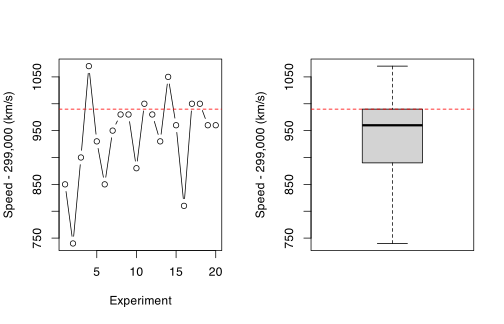
The measures fluctuate between 740 and 1,070 with no visible trend over the experiments, so treating them as identically distributed is reasonable; the distribution is roughly symmetric with a slightly longer lower tail, and most measures (the whole box) lie at or below Cornu’s value 990.
13.2- Shapiro-Wilk test (Section 13.3.3) of \(H_0\): the data are normally distributed:
shapiro.test(light)
Shapiro-Wilk normality test
data: light
W = 0.94593, p-value = 0.3095
With \(p = 0.31 > 0.05\) normality is not rejected, so a Student test is justified.
13.3- Test \(H_0: \mu = 990\) (Cornu’s \(c = 299{,}990\) km/s) against \(H_1: \mu \ne 990\) with t.test() (Section 13.3.1):
t.test(light, mu = 990)
One Sample t-test
data: light
t = -2.8189, df = 19, p-value = 0.01096
alternative hypothesis: true mean is not equal to 990
95 percent confidence interval:
901.1333 976.8667
sample estimates:
mean of x
939
With \(p = 0.011 < 0.05\) we reject \(H_0\): Michelson’s measures invalidate Cornu’s value at the 5% level (though not at the 1% level).
13.4- Michelson could propose the empirical mean, \(c \approx 299{,}939\) km/s, with the 95% Student confidence interval of Section 13.2.1:
299000 + c(estimate = mean(light), t.test(light)$conf.int)
estimate
299939.0 299901.1 299976.9
That is, \(c \approx 299{,}939\) km/s with 95% confidence interval \([299{,}901;\ 299{,}977]\) km/s.
Worksheet 13.W.C.5 — A few practical examples - Cholesterol levels
Worksheet 13.W.C.5 — A few practical examples — Cholesterol levels
Seventeen people with the same illness I are randomly assigned to two groups. The first group receives a placebo A and the second group receives a treatment B containing a vitamin. The relevant measure is capillary resistance. We get the following measurements:
Group A: 46.3 ; 42.5 ; 43.0 ; 43.9 ; 42.0 ; 41.5 ; 41.6 ; 44.4 ; 40.7
Group B: 47.1 ; 44.5 ; 45.8 ; 49.0 ; 44.6 ; 43.7 ; 44.5 ; 47.4
Assuming that the measure of capillary resistance is normally distributed, what can you conclude?
The vitamin treatment significantly increases capillary resistance (\(p = 0.004\)). The groups are independent, so compare the two means with a two-sample Student test (Section 13.3.1), after checking equality of variances with Fisher’s test var.test():
A <- c(46.3, 42.5, 43.0, 43.9, 42.0, 41.5, 41.6, 44.4, 40.7)
B <- c(47.1, 44.5, 45.8, 49.0, 44.6, 43.7, 44.5, 47.4)
var.test(A, B)$p.value
t.test(A, B, var.equal = TRUE)
[1] 0.8710977
Two Sample t-test
data: A and B
t = -3.391, df = 15, p-value = 0.004032
alternative hypothesis: true difference in means is not equal to 0
95 percent confidence interval:
-4.799753 -1.094691
sample estimates:
mean of x mean of y
42.87778 45.82500
Equal variances are not rejected (\(p = 0.87\)), and the Student test rejects \(H_0: \mu_A = \mu_B\) (\(p = 0.004 < 0.05\)): mean capillary resistance is about 2.9 units higher under treatment B (45.8 against 42.9; 95% CI for \(\mu_A - \mu_B\): \([-4.80, -1.09]\)), so the vitamin treatment is effective.
Worksheet 13.W.C.6 — A few practical examples - Treatment-death independence
Worksheet 13.W.C.6 — A few practical examples — Treatment-death independence
Two small groups of animals are infected by a virulent germ. The first group receives chemotherapy; the second group is not treated. We measure mortality after eight days in both groups.
| With treatment | Without treatment | Total | |
|---|---|---|---|
| Dead | 0 | 9 | 9 |
| Survived | 8 | 3 | 11 |
| Total | 8 | 12 | 20 |
Is mortality independent of treatment?
No: Fisher’s exact test (Section 13.3.2) rejects independence with \(p = 0.0014\). The expected counts under independence are below 5, so the \(\chi^2\) test is not valid here and fisher.test() is the right tool:
tab <- matrix(c(0, 8, 9, 3), nrow = 2,
dimnames = list(c("Dead", "Survived"), c("With", "Without")))
suppressWarnings(chisq.test(tab)$expected)
fisher.test(tab)$p.value
With Without
Dead 3.6 5.4
Survived 4.4 6.6
[1] 0.001381281
We reject \(H_0\): mortality and treatment are independent. Mortality depends on treatment: none of the 8 treated animals died, against 9 of the 12 untreated ones.
Worksheet 13.W.C.7 — A few practical examples - Number of patients in the emergency ward
Worksheet 13.W.C.7 — A few practical examples — Number of patients in the emergency ward
To study the variation of the number of emergency cases in a hospital, the number of patients was counted for the months of June, July and August. The results are:
| June | July | August | |
|---|---|---|---|
| Number of patients | 1,500 | 1,600 | 1,450 |
| Number of emergency patients | 675 | 720 | 610 |
Can we conclude that the proportion of emergency cases is the same every month?
We cannot reject that it is the same: the test of equality of several proportions, prop.test() (Section 13.3.1), does not reject \(H_0: p_{\text{June}} = p_{\text{July}} = p_{\text{August}}\) (\(p = 0.18\)):
emerg <- c(June = 675, July = 720, August = 610)
total <- c(1500, 1600, 1450)
round(emerg / total, 3)
prop.test(emerg, total)
June July August
0.450 0.450 0.421
3-sample test for equality of proportions without continuity correction
data: emerg out of total
X-squared = 3.4433, df = 2, p-value = 0.1788
alternative hypothesis: two.sided
sample estimates:
prop 1 prop 2 prop 3
0.4500000 0.4500000 0.4206897
With \(p = 0.18 > 0.05\) the observed proportions (45%, 45%, 42%) are compatible with a common proportion of emergency cases (about 44%) across the three months; the dip in August is within sampling variation. The authors’ companion solution applies chisq.test() to the three proportions themselves, which is a goodness-of-fit test on non-counts and ignores the sample sizes; prop.test() is the correct test and reaches the same conclusion.
Simple and multiple linear regression
Exercises 14.1–14.7
Give the instruction to fit the model \(Y = \beta_0 + \beta_1 X_1 + \epsilon\).
lm(Y ~ X1) (the intercept is included by default, Section 14.2). On simulated data (seed 1), reused in the following exercises:
set.seed(1)
n <- 100
X1 <- runif(n, 0, 2); X2 <- rnorm(n)
Z <- factor(sample(c("a", "b", "c"), n, replace = TRUE))
Y <- 1 + 2*X1 - X2 + 0.5*X1*X2 + (Z == "b") + rnorm(n, sd = 0.5)
X3 <- rnorm(n) # pure noise, used in 14.11-14.12
coef(lm(Y ~ X1))
(Intercept) X1
1.227759 2.081160
Give the instruction to fit the model \(Y = \beta_1 X_1 + \epsilon\).
lm(Y ~ -1 + X1) (equivalently lm(Y ~ X1 + 0)): the -1 removes the intercept.
coef(lm(Y ~ -1 + X1))
X1
3.018764
Give the instruction to fit the model \(Y = \beta_0 + \beta_1 X_1 + \beta_2 X_2 + \epsilon\).
lm(Y ~ X1 + X2) (Section 14.3).
coef(lm(Y ~ X1 + X2))
(Intercept) X1 X2
1.1301441 2.1661711 -0.5443446
Give the instruction to fit the model \(Y = \beta_0 + \beta_1 X_1 \times \beta_2 X_2 + \beta_3 X_1 + \beta_4 X_2 + \epsilon\).
lm(Y ~ X1 * X2), i.e. lm(Y ~ X1 + X2 + X1:X2) (Section 14.3.6); the printed “\(\beta_1 X_1 \times \beta_2 X_2\)” is a typo for the interaction term \(\beta_1 X_1 X_2\), and a product of two coefficients would not be identifiable.
coef(lm(Y ~ X1 * X2))
(Intercept) X1 X2 X1:X2
1.1014228 2.1782534 -0.9182888 0.3694867
Give the instruction to fit the model \(Y = \beta_0 + \beta_1 X_1 + \beta_2 X_1^2 + \beta_3 X_1^4 + \epsilon\).
lm(Y ~ X1 + I(X1^2) + I(X1^4)): I() makes ^ an arithmetic power rather than a formula operator (Section 14.3.10).
coef(lm(Y ~ X1 + I(X1^2) + I(X1^4)))
(Intercept) X1 I(X1^2) I(X1^4)
1.4025191267 1.6061815730 0.2324587625 0.0006218695
Which instruction performs a partial Fisher test?
anova(mod1, mod2), where mod1 is the sub-model nested in mod2 (Section 14.3.4, Table 14.2). Testing \(H_0: \beta_2 = \beta_3 = 0\) in \(Y = \beta_0 + \beta_1 X_1 + \beta_2 X_2 + \beta_3 X_1 X_2 + \epsilon\):
mod1 <- lm(Y ~ X1)
mod2 <- lm(Y ~ X1 + X2 + X1:X2)
anova(mod1, mod2)
Analysis of Variance Table
Model 1: Y ~ X1
Model 2: Y ~ X1 + X2 + X1:X2
Res.Df RSS Df Sum of Sq F Pr(>F)
1 98 80.038
2 96 50.770 2 29.268 27.671 3.242e-10 ***
With \(F = 27.67\) on \((2, 96)\) degrees of freedom and \(p \approx 3\times 10^{-10}\), \(H_0\) is rejected: \(X_2\) and the interaction jointly contribute to explaining \(Y\) given \(X_1\).
Which function recovers the residuals of a model?
residuals() (alias resid()), applied to the fitted lm object; rstandard() and rstudent() give the standardized and studentized versions (Section 14.3.9).
head(round(residuals(mod2), 3), 4)
1 2 3 4
0.385 -0.972 -0.235 -0.177
Exercises 14.8–14.12
Which function gives the estimates of a regression model?
coef() (alias coefficients()) returns the estimated coefficients \(\hat\beta_j\); summary(lm()) (or its $coefficients component) adds their standard errors, \(t\) statistics and \(p\)-values.
coef(mod2)
round(summary(mod2)$coefficients, 4)
(Intercept) X1 X2 X1:X2
1.1014228 2.1782534 -0.9182888 0.3694867
Estimate Std. Error t value Pr(>|t|)
(Intercept) 1.1014 0.1600 6.8820 0.000
X1 2.1783 0.1372 15.8773 0.000
X2 -0.9183 0.1641 -5.5974 0.000
X1:X2 0.3695 0.1426 2.5915 0.011
Let \(Z\) be a qualitative variable. Which function should you use to fit a regression model with \(Z\) as the explanatory variable?
factor() inside the formula, lm(Y ~ factor(Z)), so that \(Z\) is coded by indicator variables against a reference level (Section 14.3.5; relevel() changes the reference).
coef(lm(Y ~ factor(Z)))
(Intercept) factor(Z)b factor(Z)c
2.8932267 1.4785262 0.2750768
Give the instruction to fit the polynomial model \(Y = \beta_0 + \beta_1 X^1 + \beta_2 X^2 + \beta_3 X^3 + \epsilon\).
lm(Y ~ poly(X, 3, raw = TRUE)), or equivalently lm(Y ~ X + I(X^2) + I(X^3)) (Section 14.3.10); raw = TRUE gives the plain powers rather than orthogonal polynomials. With X1 as \(X\):
coef(lm(Y ~ poly(X1, 3, raw = TRUE)))
(Intercept) poly(X1, 3, raw = TRUE)1 poly(X1, 3, raw = TRUE)2
1.38012619 1.72726144 0.08161453
poly(X1, 3, raw = TRUE)3
0.05228201
Which function performs forward selection?
add1(..., test = "F"), applied repeatedly from the null model, adding at each step the most significant variable while its \(p\)-value is below \(\alpha\) (Section 14.3.8); step(..., direction = "forward") automates the search with the AIC.
add1(lm(Y ~ 1), ~ X1 + X2 + X3 + Z, test = "F")
fw <- step(lm(Y ~ 1), scope = ~ X1 + X2 + X3 + Z,
direction = "forward", trace = 0)
formula(fw)
Single term additions
Model:
Y ~ 1
Df Sum of Sq RSS AIC F value Pr(>F)
<none> 202.846 72.728
X1 1 122.809 80.038 -18.267 150.3694 < 2.2e-16 ***
X2 1 16.530 186.316 66.228 8.6947 0.00399 **
X3 1 0.000 202.846 74.728 0.0002 0.98793
Z 2 37.512 165.334 56.280 11.0041 4.931e-05 ***
Y ~ X1 + X2 + Z
\(X_1\) enters first (largest \(F\), \(p < 2.2\times 10^{-16}\)), and the automated search stops at Y ~ X1 + X2 + Z, correctly leaving out the pure-noise \(X_3\).
Which function performs backward selection?
drop1(..., test = "F"), applied repeatedly from the full model, deleting at each step the least significant variable while its \(p\)-value exceeds \(\alpha\) (Section 14.3.8); step(..., direction = "backward") automates it with the AIC.
drop1(lm(Y ~ X1 + X2 + X3 + Z), test = "F")
bw <- step(lm(Y ~ X1 + X2 + X3 + Z), direction = "backward", trace = 0)
formula(bw)
Single term deletions
Model:
Y ~ X1 + X2 + X3 + Z
Df Sum of Sq RSS AIC F value Pr(>F)
<none> 34.560 -94.248
X1 1 113.487 148.047 49.236 308.6774 < 2.2e-16 ***
X2 1 25.060 59.620 -41.718 68.1624 9.241e-13 ***
X3 1 0.028 34.588 -96.168 0.0758 0.7837
Z 2 19.739 54.299 -53.067 26.8445 5.993e-10 ***
Y ~ X1 + X2 + Z
\(X_3\) has the largest \(p\)-value (0.78) and is deleted; all remaining terms are significant, so both procedures select Y ~ X1 + X2 + Z.
Worksheet 14.W.A.1 — Study of simple linear regression - Study of synthetic data
Worksheet 14.W.A.1 — Study of simple linear regression — Study of synthetic data
14.1- Simulate a dataset \((x_i, y_i)\), \(i = 1, \ldots, n\) from a simple linear regression model. To this end:
- choose the true parameters \(\beta_0\) and \(\beta_1\), as well as \(\sigma > 0\);
- simulate the vector of errors \(e\) of size \(n\) from a normal distribution \(\mathcal{N}(0, \sigma^2)\);
- simulate the vector of values of the explanatory variable \(x\) of size \(n\) from a uniform distribution over \([0, t]\) where \(t\) is a positive real number of your choosing;
- construct the vector of values of the explained variable \(y\) of size \(n\) from the linear regression model.
14.2- Plot the \(n\) points \((x_i, y_i)\).
14.3- Give an estimate of the regression parameters and of the error variance.
14.4- Analyse the residuals to validate the model:
- plot the residuals against the fitted values;
- plot the fitted values against the observed values;
- draw a plot to check the normality of residuals.
14.5- Change the values of \(n\) and \(\sigma\) to understand the consequences on the precision of the regression parameter estimates (in terms of variance).
14.1- With \(\beta_0 = 2\), \(\beta_1 = 3\), \(\sigma = 1.5\), \(n = 50\) and \(t = 10\) (seed 1), the model \(y_i = \beta_0 + \beta_1 x_i + e_i\) is simulated by:
set.seed(1)
n <- 50; beta0 <- 2; beta1 <- 3; sigma <- 1.5; t <- 10
e <- rnorm(n, mean = 0, sd = sigma)
x <- runif(n, min = 0, max = t)
y <- beta0 + beta1 * x + e
14.2- The points lie along a straight line of slope about 3 with a roughly constant spread.
plot(x, y, pch = 19, main = "Simulated data (n = 50)")
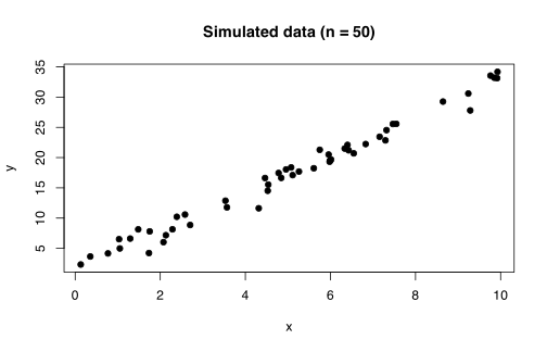
14.3- \(\hat\beta_0 = 1.53\), \(\hat\beta_1 = 3.12\) and \(\hat\sigma^2 = 1.47\) (the residual mean square, Section 14.2.2), to be compared with the true values 2, 3 and \(1.5^2 = 2.25\); with only 48 residual degrees of freedom the variance estimate is the least precise of the three.
model <- lm(y ~ x)
coef(model)
summary(model)$sigma^2
(Intercept) x
1.530688 3.124003
[1] 1.466543
14.4- The residuals scatter randomly around 0 with constant spread, the fitted values follow the line \(\hat y = y\), and the normal Q-Q plot is close to a straight line (Shapiro-Wilk \(p = 0.057\)), so the model is validated, as expected for data generated from it (Section 14.2.4).
par(mfrow = c(1, 3))
plot(fitted(model), residuals(model), xlab = "Fitted values", ylab = "Residuals")
abline(h = 0, lty = 2)
plot(y, fitted(model), xlab = "Observed values", ylab = "Fitted values")
abline(0, 1, col = "red")
qqnorm(residuals(model)); qqline(residuals(model), col = "red")
shapiro.test(residuals(model))
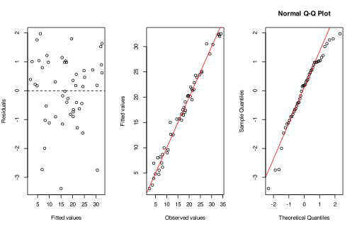
Shapiro-Wilk normality test
data: residuals(model)
W = 0.95534, p-value = 0.05673
14.5- Repeating the simulation 1000 times for each \((n, \sigma)\) (seed 1) and taking the empirical variance of the estimates shows that both variances grow like \(\sigma^2\) and shrink like \(1/n\): multiplying \(\sigma\) by 10 multiplies them by about 100, multiplying \(n\) by 25 divides them by about 25, in line with \(\operatorname{Var}(\hat\beta_1) = \sigma^2 / \sum_i (x_i - \bar x)^2\).
sim <- function(n, sigma, B = 1000, t = 10) {
est <- replicate(B, {
x <- runif(n, 0, t)
y <- 2 + 3 * x + rnorm(n, 0, sigma)
coef(lm(y ~ x))
})
apply(est, 1, var)
}
set.seed(1)
grid <- expand.grid(n = c(20, 100, 500), sigma = c(0.5, 1.5, 5))
res <- t(mapply(sim, grid$n, grid$sigma))
colnames(res) <- c("var(b0)", "var(b1)")
cbind(grid, signif(res, 3))
n sigma var(b0) var(b1)
1 20 0.5 0.05060 1.60e-03
2 100 0.5 0.01090 3.41e-04
3 500 0.5 0.00204 6.07e-05
4 20 1.5 0.46800 1.44e-02
5 100 1.5 0.08710 2.51e-03
6 500 1.5 0.01780 5.35e-04
7 20 5.0 5.29000 1.51e-01
8 100 5.0 0.99800 2.96e-02
9 500 5.0 0.21500 6.53e-03
Worksheet 14.W.A.2 — Study of simple linear regression - Study of intima-media
Worksheet 14.W.A.2 — Study of simple linear regression — Study of intima-media
In the “Intima-media” study, we wish to study the relationship between intima-media thickness and age.
14.1- Download the intima-media data file.
14.2- Plot variable measure as a function of variable AGE. Describe this scatter plot.
14.3- Is there a link between these variables? Explain how to measure the severeness of the link.
14.4- We now wish to fit a regression line on this scatter plot:
- propose a regression model and estimate the parameters of the model;
- draw the regression line over the scatter plot.
14.5- Analyse the residuals to validate the model.
14.6- Give a prediction interval for intima-media thickness for a 33 years old person.
14.7- Give a confidence interval for the average intima-media thickness of 33 years old people.
14.8- Propose a model to increase the predictive power of intima-media thickness, using only AGE as an explanatory variable.
14.1- The file uses single spaces as separators (empty fields are missing values) and a decimal comma, so it is read with sep = " " and dec = ",":
url <- "http://www.biostatisticien.eu/springeR/Intima_Media_Thickness.txt"
intima <- read.table(url, header = TRUE, sep = " ", dec = ",")
str(intima[, c("AGE", "measure")])
'data.frame': 110 obs. of 2 variables:
$ AGE : int 33 33 53 42 53 50 22 26 50 47 ...
$ measure: num 0.52 0.42 0.65 0.48 0.45 0.49 0.42 0.45 0.65 0.52 ...
14.2- The cloud of the 110 subjects (aged 22 to 64, thickness 0.40 to 0.82 mm) rises with age and fans out: thickness is tightly grouped around 0.45-0.50 mm before 35 and much more dispersed, with several high values, after 45.
plot(measure ~ AGE, data = intima, pch = 19,
xlab = "Age (years)", ylab = "Intima-media thickness (mm)")
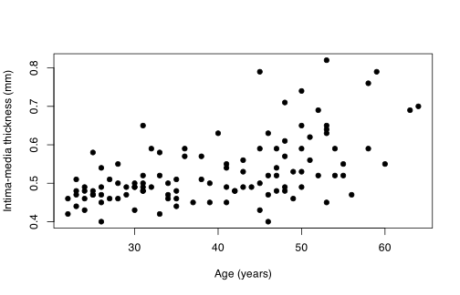
14.3- Yes: the link is positive and roughly linear. Its strength is measured by Pearson’s linear correlation coefficient \(r = 0.55\), and \(H_0: \rho = 0\) is rejected (\(p = 4 \times 10^{-10}\)); equivalently \(R^2 = r^2 = 0.31\) of the variability of thickness is explained by age.
cor.test(~ AGE + measure, data = intima)
Pearson's product-moment correlation
data: AGE and measure
t = 6.8862, df = 108, p-value = 3.953e-10
alternative hypothesis: true correlation is not equal to 0
95 percent confidence interval:
0.4072451 0.6702836
sample estimates:
cor
0.5523669
14.4- The model is \(\text{measure}_i = \beta_0 + \beta_1 \text{AGE}_i + \epsilon_i\) with \(\epsilon_i\) i.i.d. \(\mathcal{N}(0, \sigma^2)\) (Section 14.2). The fit gives \(\hat\beta_0 = 0.361\) mm, \(\hat\beta_1 = 0.00429\) mm per year (about 0.043 mm per decade, significantly non-zero, \(p = 4 \times 10^{-10}\)) and \(\hat\sigma = 0.0726\).
model <- lm(measure ~ AGE, data = intima)
summary(model)
plot(measure ~ AGE, data = intima, pch = 19)
abline(model, col = "red", lwd = 2)
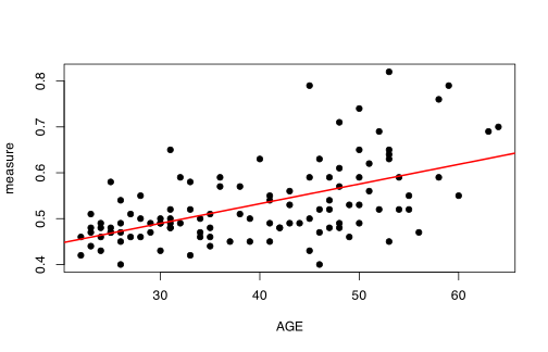
Coefficients:
Estimate Std. Error t value Pr(>|t|)
(Intercept) 0.3610255 0.0255330 14.140 < 2e-16 ***
AGE 0.0042897 0.0006229 6.886 3.95e-10 ***
...
Residual standard error: 0.07257 on 108 degrees of freedom
Multiple R-squared: 0.3051, Adjusted R-squared: 0.2987
F-statistic: 47.42 on 1 and 108 DF, p-value: 3.953e-10
(output truncated to the coefficient table and fit summary)
14.5- The model is only partly validated. The residuals are centred with no strong trend, but their spread grows with the fitted values (Scale-Location plot; Breusch-Pagan \(p = 0.0004\)), and the Q-Q plot bends upwards at the right with subjects 39, 81, 92 standing out, so the residuals are right-skewed rather than normal (Shapiro-Wilk \(p = 0.002\)). No point has a large leverage or Cook’s distance (Section 14.2.4), so the line itself is trustworthy, but intervals based on normality with constant variance should be read with caution.
par(mfrow = c(2, 2))
plot(model)
shapiro.test(residuals(model))
library(lmtest)
bptest(model)
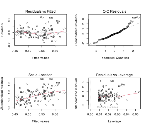
Shapiro-Wilk normality test
data: residuals(model)
W = 0.95936, p-value = 0.002005
studentized Breusch-Pagan test
data: model
BP = 12.51, df = 1, p-value = 0.0004048
14.6- A 95% prediction interval for the thickness of one 33-year-old is \([0.358, 0.647]\) mm, around the prediction \(0.503\) mm (Section 14.2.3).
new <- data.frame(AGE = 33)
predict(model, new, interval = "prediction")
fit lwr upr
1 0.5025848 0.3578677 0.647302
14.7- A 95% confidence interval for the mean thickness of 33-year-olds is \([0.487, 0.518]\) mm, much narrower than the prediction interval because it ignores the individual error \(\epsilon\).
predict(model, new, interval = "confidence")
fit lwr upr
1 0.5025848 0.4867222 0.5184474
14.8- Since the cloud curves upwards after 45, a polynomial regression in AGE (Section 14.3.10), \(\text{measure} = \beta_0 + \beta_1 \text{AGE} + \beta_2 \text{AGE}^2 + \epsilon\), is proposed. It raises the adjusted \(R^2\) from 0.299 to 0.315, although the quadratic term is only borderline (partial Fisher test \(p = 0.061\)), and a cubic term brings nothing more (\(p = 0.41\)).
model2 <- lm(measure ~ poly(AGE, 2, raw = TRUE), data = intima)
model3 <- lm(measure ~ poly(AGE, 3, raw = TRUE), data = intima)
anova(model, model2)
anova(model2, model3)
sapply(list(model, model2, model3), function(m) summary(m)$adj.r.squared)
Analysis of Variance Table
Model 1: measure ~ AGE
Model 2: measure ~ poly(AGE, 2, raw = TRUE)
Res.Df RSS Df Sum of Sq F Pr(>F)
1 108 0.56876
2 107 0.55031 1 0.018452 3.5878 0.06091 .
...
Analysis of Variance Table
Model 1: measure ~ poly(AGE, 2, raw = TRUE)
Model 2: measure ~ poly(AGE, 3, raw = TRUE)
Res.Df RSS Df Sum of Sq F Pr(>F)
1 107 0.55031
2 106 0.54684 1 0.003473 0.6732 0.4138
[1] 0.2986750 0.3150862 0.3129880
Worksheet 14.W.B.1 — Study of multiple linear regression - Study of intima-media
Worksheet 14.W.B.1 — Study of multiple linear regression — Study of intima-media
In the previous practical, we looked at the relationship between intima-media thickness and age. We now wish to fit a regression model on all variables which may explain variations in intima-media thickness. The study will rely on the following variables: AGE, SPORT, alcohol, packyear and the variable BMI which you must create from variables height, weight.
We are mostly interested in tobacco, through the variable packyear as main exposure factor. We therefore decide to keep this variable in the model even if it is not significant.
14.1- Draw scatter plots of all pairs of variables (explained and explanatory). Do you suspect any issues with collinearity?
14.2- Perform a univariate analysis of intima-media thickness of each explanatory variable.
14.3- We only keep the explanatory variables associated with significance level \(p < 0.25\) in the univariate analysis. One by one, test all possible interactions between the selected explanatory variables and the main exposure variable packyear.
14.4- Estimate and analyse the model with all variables which were declared significant in the univariate analyses (\(\alpha = 25\%\)) and all interaction terms significant at the 10% level.
14.5- Are the interaction terms still significant? Remove interaction terms which are no longer significant at the 10% level.
14.6- Starting with the model from the previous question, remove one by one all variables which are not significant at the 5% level, making sure that the removals do not make a big difference on the estimate of the coefficient associated with tobacco status.
14.7- Interpret the final model.
Read the intima-media file of Worksheet A with read.table() (Chapter 4); packyear is NA exactly for the 72 non-smokers (tobacco = 0), so it is set to 0, BMI is weight (kg) over squared height (m), and alcohol (coded 0, 1, 2) is a factor.
url <- "http://www.biostatisticien.eu/springeR/Intima_Media_Thickness.txt"
im <- read.table(url, header = TRUE, sep = " ", dec = ",")
table(tobacco = im$tobacco, packyear.NA = is.na(im$packyear))
im$packyear[is.na(im$packyear)] <- 0
im$BMI <- im$weight / (im$height / 100)^2
my.data <- data.frame(AGE = im$AGE, SPORT = im$SPORT,
alcohol = factor(im$alcohol), packyear = im$packyear,
BMI = im$BMI, measure = im$measure)
packyear.NA
tobacco FALSE TRUE
0 0 72
1 18 0
2 20 0
14.1- pairs() draws every pairwise scatter plot; the correlation matrix quantifies what it shows.
pairs(my.data, pch = 20, cex = 0.6)
round(cor(data.matrix(my.data)), 2)
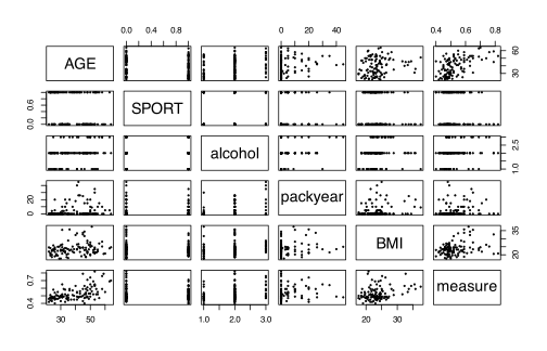
AGE SPORT alcohol packyear BMI measure
AGE 1.00 -0.17 0.24 0.19 0.18 0.55
SPORT -0.17 1.00 0.03 -0.06 -0.13 -0.10
alcohol 0.24 0.03 1.00 0.26 0.15 0.24
packyear 0.19 -0.06 0.26 1.00 0.17 0.15
BMI 0.18 -0.13 0.15 0.17 1.00 0.31
measure 0.55 -0.10 0.24 0.15 0.31 1.00
The measure row shows a clear linear trend with AGE (\(r = 0.55\)) and a weaker one with BMI (\(0.31\)). Some pairs of explanatory variables show mild linear trends (AGE, alcohol and packyear are pairwise correlated at about 0.2 to 0.26), so a little collinearity is present, but every correlation between regressors is below 0.3: no serious collinearity problem is expected (this will be confirmed by the stability of the estimates below).
14.2- Fit one simple regression (one-way ANOVA for the factor alcohol) per explanatory variable and collect the \(p\)-value of its overall \(F\) test:
vars <- c("AGE", "SPORT", "alcohol", "packyear", "BMI")
p.uni <- sapply(vars, function(v)
anova(lm(reformulate(v, "measure"), data = my.data))[1, "Pr(>F)"])
round(p.uni, 4)
AGE SPORT alcohol packyear BMI
0.0000 0.3072 0.0448 0.1108 0.0011
Taken one at a time, AGE (\(p < 10^{-4}\)), BMI (\(p = 0.001\)) and alcohol (\(p = 0.045\)) are significantly associated with intima-media thickness at the 5% level, packyear is not (\(p = 0.11\)), and SPORT shows no association (\(p = 0.31\)).
14.3- At the 25% level we keep AGE, alcohol, BMI and packyear and drop SPORT. Each interaction with packyear is tested by a partial Fisher test (Section 14.3.4) comparing the additive model with the model containing the interaction:
p.inter <- sapply(c("AGE", "alcohol", "BMI"), function(v) {
m0 <- lm(reformulate(c(v, "packyear"), "measure"), data = my.data)
m1 <- lm(reformulate(paste0(v, "*packyear"), "measure"), data = my.data)
anova(m0, m1)[2, "Pr(>F)"]
})
round(p.inter, 4)
round(coef(summary(lm(measure ~ alcohol * packyear, data = my.data)))[5:6, ], 4)
AGE alcohol BMI
0.7453 0.1031 0.5473
Estimate Std. Error t value Pr(>|t|)
alcohol1:packyear -0.0048 0.0031 -1.5633 0.1210
alcohol2:packyear -0.0066 0.0031 -2.1373 0.0349
The AGE:packyear and BMI:packyear interactions are clearly not significant. The alcohol:packyear interaction is borderline: its global test gives \(p = 0.103\), but the coefficient for heavy drinkers (alcohol2:packyear) has \(p = 0.035 < 0.10\), so we retain this interaction for the next step (as does the authors’ companion solution).
14.4- The model contains AGE, BMI, alcohol, packyear and the alcohol:packyear interaction:
model.inter <- lm(measure ~ AGE + BMI + alcohol * packyear, data = my.data)
summary(model.inter)
Coefficients:
Estimate Std. Error t value Pr(>|t|)
(Intercept) 0.2640114 0.0468079 5.640 1.52e-07 ***
AGE 0.0037386 0.0006504 5.748 9.44e-08 ***
BMI 0.0042187 0.0018080 2.333 0.0216 *
alcohol1 0.0185379 0.0187008 0.991 0.3239
alcohol2 0.0409030 0.0277387 1.475 0.1434
packyear 0.0028237 0.0024036 1.175 0.2428
alcohol1:packyear -0.0025591 0.0026442 -0.968 0.3354
alcohol2:packyear -0.0036977 0.0026613 -1.389 0.1677
...
Residual standard error: 0.07119 on 102 degrees of freedom
Multiple R-squared: 0.3685, Adjusted R-squared: 0.3252
F-statistic: 8.503 on 7 and 102 DF, p-value: 3.589e-08
(Call, residual quantiles and significance codes truncated.) The model is globally significant (\(F = 8.50\) on 7 and 102 df, \(p = 3.6 \times 10^{-8}\)) and explains 37% of the variance; once adjusted for the other variables, only AGE and BMI have significant coefficients.
14.5- No: in the adjusted model neither interaction coefficient is significant (\(p = 0.34\) and \(0.17\)), and the partial Fisher test of both together gives \(p = 0.37\), so the interaction is removed.
model.without.inter <- lm(measure ~ AGE + BMI + alcohol + packyear, data = my.data)
anova(model.without.inter, model.inter)
round(coef(summary(model.without.inter)), 5)
Analysis of Variance Table
Model 1: measure ~ AGE + BMI + alcohol + packyear
Model 2: measure ~ AGE + BMI + alcohol * packyear
Res.Df RSS Df Sum of Sq F Pr(>F)
1 104 0.52700
2 102 0.51688 2 0.010127 0.9993 0.3717
Estimate Std. Error t value Pr(>|t|)
(Intercept) 0.25938 0.04637 5.59416 0.00000
AGE 0.00385 0.00064 5.98157 0.00000
BMI 0.00451 0.00178 2.53417 0.01276
alcohol1 0.01309 0.01729 0.75736 0.45055
alcohol2 0.02397 0.02471 0.97007 0.33426
packyear 0.00000 0.00078 -0.00150 0.99881
14.6- packyear is kept by design, so the only candidate for removal is alcohol (both of its coefficients have \(p > 0.3\)); a partial Fisher test compares the models with and without it:
model.final <- lm(measure ~ AGE + BMI + packyear, data = my.data)
anova(model.final, model.without.inter)
rbind(with.alcohol = coef(model.without.inter)["packyear"],
without.alcohol = coef(model.final)["packyear"])
Analysis of Variance Table
Model 1: measure ~ AGE + BMI + packyear
Model 2: measure ~ AGE + BMI + alcohol + packyear
Res.Df RSS Df Sum of Sq F Pr(>F)
1 106 0.53209
2 104 0.52700 2 0.0050855 0.5018 0.6069
packyear
with.alcohol -1.167391e-06
without.alcohol 1.549257e-04
alcohol adds nothing once AGE, BMI and packyear are in the model (\(p = 0.61\)), so it is removed. The packyear coefficient moves from \(-0.000001\) to \(0.00015\) mm per pack-year, a change that is tiny compared with its standard error (0.00076), so the removal does not alter the tobacco estimate. AGE and BMI remain significant at 5%, so the procedure stops.
14.7- The final model is \(\text{measure} = \beta_0 + \beta_1\,\text{AGE} + \beta_2\,\text{BMI} + \beta_3\,\text{packyear} + \epsilon\):
summary(model.final)
round(confint(model.final), 5)
Coefficients:
Estimate Std. Error t value Pr(>|t|)
(Intercept) 0.2623458 0.0451913 5.805 6.77e-08 ***
AGE 0.0039677 0.0006272 6.325 6.14e-09 ***
BMI 0.0046588 0.0017665 2.637 0.00962 **
packyear 0.0001549 0.0007559 0.205 0.83800
...
Residual standard error: 0.07085 on 106 degrees of freedom
Multiple R-squared: 0.3499, Adjusted R-squared: 0.3315
F-statistic: 19.02 on 3 and 106 DF, p-value: 6.087e-10
2.5 % 97.5 %
(Intercept) 0.17275 0.35194
AGE 0.00272 0.00521
BMI 0.00116 0.00816
packyear -0.00134 0.00165
(Call, residual quantiles and significance codes truncated.) Intima-media thickness is explained by AGE and BMI, adjusted for tobacco exposure: whatever the number of pack-years smoked, the thickness increases on average by 0.0040 mm per year of age (95% CI 0.0027 to 0.0052), i.e. about 0.04 mm per decade, and by 0.0047 mm per unit of BMI (95% CI 0.0012 to 0.0082). Adjusted for age and BMI, tobacco has no detectable effect (\(p = 0.84\), CI \([-0.0013, 0.0017]\) mm per pack-year): its weak crude association (\(r = 0.15\)) is absorbed by age, which is correlated with both. The model explains 35% of the variability of the thickness.
Worksheet 14.W.B.2 — Study of multiple linear regression - Study of unemployment rates
Worksheet 14.W.B.2 — Study of multiple linear regression — Study of unemployment rates
This practical studies unemployment rates from 1960 to 1993. The dataset unemployment is made of \(n = 34\) yearly observations (from 1960 to 1993). Here is a description of the variables:
year: year;unemp: unemployment rate;gdprate: rate of variation of Gross domestic product (GDP), representing economic growth;govspend: ratio of government spending and GDP, representing the degree of intervention of the state in the economy;taxb: tax burden, to see whether taxation of businesses has an impact on hiring policy, and hence on unemployment rates;salav: ratio of salaries to added value, to know the influence of cost at hiring;infl: inflation rate, to verify the inverse relationship between unemployment and inflation, defined in the Philips curve.
14.1- We consider a linear model explaining variable unemp as a function of variable gdprate only. Download the dataset http://www.biostatisticien.eu/springeR/unemployment.RData. Perform a complete analysis of the underlying simple linear regression model.
14.2- We consider a multiple linear model explaining variable unemp as a function of all explanatory variables in the dataset (except variable year). Give the correlation matrix of all these variables.
14.3- Draw scatter plots of all pairs of variables.
14.4- Which explanatory variables seem to make the biggest contribution? Do you suspect collinearity between regressors?
14.5- Present the results of the multiple linear regression model with explanatory variables.
14.6- Calculate the VIF associated with each explanatory variable.
14.7- Perform backward variable selection with threshold \(\alpha = 0.2\).
14.8- Present the final model.
14.9- Suppose we do not know the value of unemp in 1993. Can you predict its value, and calculate a 95% prediction interval?
14.10- What is the observed value of unemp in 1993? Is this surprising?
C- Study of polynomial regression — Study of synthetic data
14.1- Simulate a sample of size \(n = 100\) from the following model:
\begin{equation*} Y = X + 2X^2 + 3.5X^3 - 2.3X^4 + \epsilon \end{equation*}
where \(X\) follows a uniform distribution over \([-2, +2]\) and \(\epsilon\) follows a \(\mathcal{N}(0, 1)\) distribution.
14.2- Draw the scatter plot and the simulated polynomial line.
14.3- Fit a simple linear regression model. Remember to analyse the residuals.
14.4- Fit a polynomial regression, using a polynomial of degree 4. Draw the estimated model over the scatter plot.
14.1- The model is \(\text{unemp}_i = \beta_0 + \beta_1\,\text{gdprate}_i + \epsilon_i\); load the file with load(), then fit it with lm() and validate it with the residual plots of Section 14.2:
load(url("http://www.biostatisticien.eu/springeR/unemployment.RData"))
model.gdprate <- lm(unemp ~ gdprate, data = unemployment)
summary(model.gdprate)
confint(model.gdprate)
Coefficients:
Estimate Std. Error t value Pr(>|t|)
(Intercept) 10.0996 0.8293 12.18 1.48e-13 ***
gdprate -1.3304 0.2069 -6.43 3.14e-07 ***
...
Residual standard error: 2.381 on 32 degrees of freedom
Multiple R-squared: 0.5637, Adjusted R-squared: 0.5501
F-statistic: 41.34 on 1 and 32 DF, p-value: 3.144e-07
2.5 % 97.5 %
(Intercept) 8.410412 11.7888025
gdprate -1.751865 -0.9089548
(Call, residual quantiles and significance codes truncated.) Growth has a highly significant negative effect (\(H_0: \beta_1 = 0\) rejected, \(p = 3 \times 10^{-7}\)): each extra point of GDP growth goes with 1.33 points less unemployment (95% CI \([-1.75, -0.91]\)), and the model explains 56% of the variance.
par(mfrow = c(1, 3))
plot(unemp ~ gdprate, data = unemployment, pch = 20)
abline(model.gdprate, col = "blue")
plot(model.gdprate, which = 1:2)
shapiro.test(residuals(model.gdprate))$p.value
lmtest::dwtest(model.gdprate)$p.value
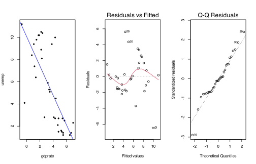
[1] 0.3019621
[1] 8.392195e-06
The residuals are compatible with normality (Shapiro-Wilk \(p = 0.30\)), but the residuals-versus-fitted plot shows a wave rather than a horizontal band and the Durbin-Watson test (\(p = 8 \times 10^{-6}\)) detects strong positive autocorrelation of these yearly residuals: the model is misspecified (unemployment trends upwards over the period for reasons growth alone does not capture), so its standard errors and \(p\)-values are over-optimistic, which motivates the multiple model.
14.2- cor() on columns 2 to 7 (all but year):
round(cor(unemployment[, 2:7]), 2)
unemp gdprate govspend taxb salav infl
unemp 1.00 -0.75 0.98 0.98 -0.17 -0.05
gdprate -0.75 1.00 -0.78 -0.75 -0.11 -0.30
govspend 0.98 -0.78 1.00 0.99 -0.01 0.07
taxb 0.98 -0.75 0.99 1.00 -0.04 0.07
salav -0.17 -0.11 -0.01 -0.04 1.00 0.70
infl -0.05 -0.30 0.07 0.07 0.70 1.00
14.3- pairs():
pairs(unemployment[, 2:7], pch = 20)
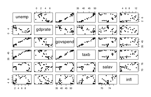
14.4- govspend and taxb (\(r = 0.98\) with unemp) and then gdprate (\(r = -0.75\)) seem to contribute most; salav and infl are almost uncorrelated with unemp. Collinearity is strongly suspected: govspend and taxb are almost perfectly correlated (\(r = 0.99\), the points lie on a line in the scatter plot), both are correlated with gdprate (\(r \approx -0.75\) to \(-0.78\)), and salav and infl are correlated (\(r = 0.70\)).
14.5- The model is \(\text{unemp} = \beta_0 + \beta_1\,\text{gdprate} + \beta_2\,\text{govspend} + \beta_3\,\text{taxb} + \beta_4\,\text{salav} + \beta_5\,\text{infl} + \epsilon\):
full.model <- lm(unemp ~ gdprate + govspend + taxb + salav + infl,
data = unemployment)
summary(full.model)
Coefficients:
Estimate Std. Error t value Pr(>|t|)
(Intercept) -5.80283 3.86147 -1.503 0.144098
gdprate -0.07188 0.07753 -0.927 0.361820
govspend 0.35855 0.12702 2.823 0.008665 **
taxb 0.22751 0.14324 1.588 0.123432
salav -0.19195 0.05079 -3.779 0.000757 ***
infl -0.03131 0.03961 -0.791 0.435873
...
Residual standard error: 0.469 on 28 degrees of freedom
Multiple R-squared: 0.9852, Adjusted R-squared: 0.9826
F-statistic: 372.7 on 5 and 28 DF, p-value: < 2.2e-16
(Call, residual quantiles and significance codes truncated.) The model is globally highly significant (\(F = 372.7\), \(p < 2.2 \times 10^{-16}\)) and explains 98.5% of the variance. Adjusted for the others, only govspend (positive effect) and salav (negative effect) are significant at 5%; gdprate, strongly significant alone in 14.1, is no longer significant (\(p = 0.36\)) because its information is carried by the correlated govspend and taxb, and taxb itself is not significant (\(p = 0.12\)) despite \(r = 0.98\) with unemp, a symptom of collinearity.
14.6- vif() from package car (Section 14.3.7):
library(car)
round(vif(full.model), 2)
gdprate govspend taxb salav infl
3.62 91.78 81.14 2.38 2.71
govspend (VIF 91.8) and taxb (VIF 81.1) are far above the usual threshold of 10: the variance of their estimates is inflated about 80 to 90 times by their collinearity, confirming 14.4; the other three VIFs are small.
14.7- Backward selection (Section 14.3.8) repeatedly applies drop1(..., test = "F") and removes the variable with the largest partial-\(F\) \(p\)-value while it exceeds 0.2:
model <- full.model
repeat {
tab <- drop1(model, test = "F")[-1, c("F value", "Pr(>F)")]
print(data.frame(F = round(tab[, 1], 3), p = signif(tab[, 2], 3),
row.names = rownames(tab)))
worst <- rownames(tab)[which.max(tab[, "Pr(>F)"])]
if (max(tab[, "Pr(>F)"]) <= 0.2) break
cat("-> remove", worst, "\n\n")
model <- update(model, as.formula(paste(". ~ . -", worst)))
}
F p
gdprate 0.859 0.362000
govspend 7.968 0.008660
taxb 2.523 0.123000
salav 14.282 0.000757
infl 0.625 0.436000
-> remove infl
F p
gdprate 0.398 5.33e-01
govspend 11.718 1.86e-03
taxb 1.984 1.70e-01
salav 43.079 3.44e-07
-> remove gdprate
F p
govspend 15.875 3.99e-04
taxb 1.714 2.00e-01
salav 43.597 2.62e-07
-> remove taxb
F p
govspend 1826.785 4.01e-29
salav 48.863 7.61e-08
infl, then gdprate, then taxb (by a hair: \(p = 0.2005\)) are removed; govspend and salav are both kept.
14.8- The final model is \(\text{unemp} = \beta_0 + \beta_1\,\text{govspend} + \beta_2\,\text{salav} + \epsilon\):
final.model <- lm(unemp ~ govspend + salav, data = unemployment)
summary(final.model)
confint(final.model)
Coefficients:
Estimate Std. Error t value Pr(>|t|)
(Intercept) -2.83284 2.46623 -1.149 0.259
govspend 0.56373 0.01319 42.741 < 2e-16 ***
salav -0.22872 0.03272 -6.990 7.61e-08 ***
...
Residual standard error: 0.4665 on 31 degrees of freedom
Multiple R-squared: 0.9838, Adjusted R-squared: 0.9827
F-statistic: 940.2 on 2 and 31 DF, p-value: < 2.2e-16
2.5 % 97.5 %
(Intercept) -7.8627567 2.1970816
govspend 0.5368330 0.5906335
salav -0.2954518 -0.1619867
(Call, residual quantiles and significance codes truncated.) With only two regressors the model still explains 98.4% of the variance (adjusted \(R^2\) 0.983, as high as the full model’s). Other things being equal, one more point of government spending in GDP goes with 0.56 more points of unemployment (95% CI \([0.54, 0.59]\)), and one more point of the share of salaries in added value with 0.23 fewer points (95% CI \([-0.30, -0.16]\)).
14.9- Yes: refit the final model without 1993 (as if unemp were unknown that year) and use predict(..., interval = "prediction") (Section 14.3.3) at the 1993 values of govspend and salav:
model.92 <- lm(unemp ~ govspend + salav, data = unemployment,
subset = year < 1993)
new93 <- unemployment[unemployment$year == 1993, c("govspend", "salav")]
new93
predict(model.92, newdata = new93, interval = "prediction")
govspend salav
34 52.2 68.6
fit lwr upr
34 10.84117 9.783461 11.89887
The predicted 1993 unemployment rate is 10.8%, with 95% prediction interval \([9.8\%, 11.9\%]\). (Predicting with final.model, fitted on all 34 years as in the book’s solution, gives 10.9%, interval \([9.9\%, 11.9\%]\).)
14.10- The observed value is 11.2%:
unemployment[unemployment$year >= 1990, ]
year unemp gdprate govspend taxb salav infl
31 1990 8.9 2.2 50.3 48.9 69.6 3.1
32 1991 9.4 1.1 50.6 48.7 69.6 3.1
33 1992 10.2 1.9 51.3 48.5 68.8 2.9
34 1993 11.2 -0.7 52.2 49.0 68.6 2.9
It is not surprising: 11.2% lies inside the 95% prediction interval \([9.8, 11.9]\), only 0.36 points above the prediction, even though 1993 was a recession year (gdprate \(= -0.7\)) that the model sees only through the rise in govspend.
C- Study of polynomial regression — Study of synthetic data
14.1- Draw \(X\) with runif() and \(\epsilon\) with rnorm() (seed 1):
set.seed(1)
n <- 100
x <- runif(n, min = -2, max = 2)
eps <- rnorm(n)
y <- x + 2 * x^2 + 3.5 * x^3 - 2.3 * x^4 + eps
summary(y)
Min. 1st Qu. Median Mean 3rd Qu. Max.
-53.6361 -2.1966 0.4616 -2.6843 3.8145 7.9844
14.2- plot() for the points and curve(..., add = TRUE) for the true polynomial:
plot(y ~ x, pch = 20)
curve(x + 2 * x^2 + 3.5 * x^3 - 2.3 * x^4, add = TRUE, col = "red", lwd = 2)
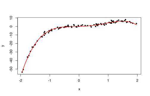
14.3- The simple linear model \(Y = \beta_0 + \beta_1 X + \epsilon\) is fitted with lm(y ~ x):
simple.model <- lm(y ~ x)
summary(simple.model)
shapiro.test(residuals(simple.model))$p.value
par(mfrow = c(1, 2))
plot(simple.model, which = 1:2)
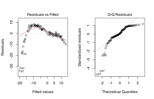
Coefficients:
Estimate Std. Error t value Pr(>|t|)
(Intercept) -3.2890 0.7382 -4.455 2.23e-05 ***
x 8.4705 0.6916 12.247 < 2e-16 ***
...
Residual standard error: 7.366 on 98 degrees of freedom
Multiple R-squared: 0.6048, Adjusted R-squared: 0.6008
F-statistic: 150 on 1 and 98 DF, p-value: < 2.2e-16
[1] 6.072915e-10
(Call, residual quantiles and significance codes truncated.) The slope is highly significant and \(R^2 = 0.60\), yet the model is wrong: the residuals-versus-fitted plot shows a strong curved pattern instead of a horizontal band, the Q-Q plot a long left tail, and the Shapiro-Wilk test rejects normality (\(p = 6 \times 10^{-10}\)); the residual standard error (7.37) is far above the true \(\sigma = 1\).
14.4- The degree-4 model without intercept, \(Y = \beta_1 X + \beta_2 X^2 + \beta_3 X^3 + \beta_4 X^4 + \epsilon\), is lm(y ~ -1 + poly(x, 4, raw = TRUE)) (Section 14.3.10):
poly.model <- lm(y ~ -1 + poly(x, 4, raw = TRUE))
summary(poly.model)
b <- coef(poly.model)
plot(y ~ x, pch = 20)
curve(b[1] * x + b[2] * x^2 + b[3] * x^3 + b[4] * x^4, add = TRUE,
col = "blue", lwd = 2)
curve(x + 2 * x^2 + 3.5 * x^3 - 2.3 * x^4, add = TRUE, col = "red",
lty = 2, lwd = 2)
legend("bottomright", c("estimated", "true"), col = c("blue", "red"),
lty = 1:2, lwd = 2)
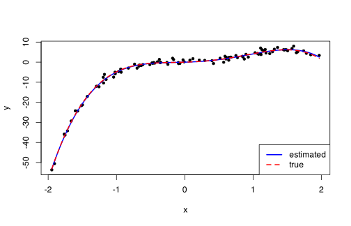
Coefficients:
Estimate Std. Error t value Pr(>|t|)
poly(x, 4, raw = TRUE)1 1.00522 0.20608 4.878 4.25e-06 ***
poly(x, 4, raw = TRUE)2 1.79451 0.19309 9.294 4.90e-15 ***
poly(x, 4, raw = TRUE)3 3.53967 0.08800 40.223 < 2e-16 ***
poly(x, 4, raw = TRUE)4 -2.22662 0.07057 -31.554 < 2e-16 ***
...
Residual standard error: 0.9444 on 96 degrees of freedom
Multiple R-squared: 0.994, Adjusted R-squared: 0.9937
F-statistic: 3950 on 4 and 96 DF, p-value: < 2.2e-16
(Call, residual quantiles and significance codes truncated.) The estimates \((1.01, 1.79, 3.54, -2.23)\) are close to the true \((1, 2, 3.5, -2.3)\), the residual standard error 0.94 matches \(\sigma = 1\), and the estimated curve is almost indistinguishable from the true one over the scatter plot.
Worksheet 14.W.B.3 — Study of multiple linear regression - Fitting a scatter plot with a polynomial
Worksheet 14.W.B.3 — Study of multiple linear regression — Fitting a scatter plot with a polynomial
Suppose you are asked to propose a model to predict a variable \(Y\) given an explanatory variable \(X\). You are given a sample of size \(n\).
14.1- Download the data file http://www.biostatisticien.eu/springeR/fitpoly.RData.
14.2- Draw a scatter plot of variable \(Y\) as a function of variable \(X\).
14.3- Is there a linear relationship between these two variables? Fit a regression line on the previous plot.
14.4- Perform polynomial regression to fit the data better.
14.5- Draw the estimated polynomial over the scatter plot. Draw the confidence curve for the mean of \(Y\) for \(X \in [-3.5, 3.5]\). Add the prediction interval of the model for \(X \in [-3.5, 3.5]\).
14.1- load() the file straight from its URL; it contains the data frame fitpoly with \(n = 100\) pairs \((X, Y)\):
load(url("http://www.biostatisticien.eu/springeR/fitpoly.RData"))
head(fitpoly, 3)
dim(fitpoly)
Y X
1 16.25158 1.077938
2 32.40916 2.339643
3 -33.41027 -2.301348
[1] 100 2
14.2- A formula in plot():
plot(Y ~ X, data = fitpoly, pch = 20)
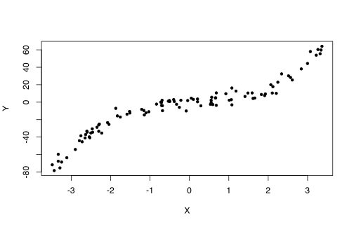
14.3- Not really: \(Y\) increases with \(X\), but along an S-shaped curve (flat near 0, steep at both ends), so a straight line is only a first approximation.
lin.model <- lm(Y ~ X, data = fitpoly)
summary(lin.model)
par(mfrow = c(1, 2))
plot(Y ~ X, data = fitpoly, pch = 20)
abline(lin.model, col = "blue", lwd = 2)
plot(lin.model, which = 1)
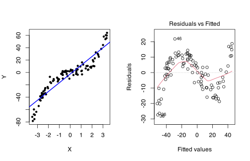
Coefficients:
Estimate Std. Error t value Pr(>|t|)
(Intercept) -2.3948 1.0840 -2.209 0.0295 *
X 14.1570 0.5471 25.876 <2e-16 ***
...
Residual standard error: 10.76 on 98 degrees of freedom
Multiple R-squared: 0.8723, Adjusted R-squared: 0.871
F-statistic: 669.5 on 1 and 98 DF, p-value: < 2.2e-16
(Call, residual quantiles and significance codes truncated.) The slope is highly significant and \(R^2 = 0.87\), but the residuals follow a clear systematic wave (negative at the left end, positive for moderately negative \(X\), negative for moderately positive \(X\), positive again at the right end), so the linear model is inadequate.
14.4- Polynomials of increasing degree are fitted with poly(X, k, raw = TRUE) (Section 14.3.10) and compared by partial Fisher tests on the nested models:
m2 <- lm(Y ~ poly(X, 2, raw = TRUE), data = fitpoly)
poly.model <- lm(Y ~ poly(X, 3, raw = TRUE), data = fitpoly)
m4 <- lm(Y ~ poly(X, 4, raw = TRUE), data = fitpoly)
anova(lin.model, m2, poly.model, m4)
summary(poly.model)
Res.Df RSS Df Sum of Sq F Pr(>F)
1 98 11337.0
2 97 10879.5 1 457.5 20.2334 1.939e-05 ***
3 96 2237.3 1 8642.2 382.1794 < 2.2e-16 ***
4 95 2148.2 1 89.1 3.9382 0.05009 .
...
Coefficients:
Estimate Std. Error t value Pr(>|t|)
(Intercept) -0.5513 0.7071 -0.780 0.43750
poly(X, 3, raw = TRUE)1 3.2447 0.6117 5.305 7.23e-07 ***
poly(X, 3, raw = TRUE)2 -0.4425 0.1328 -3.331 0.00123 **
poly(X, 3, raw = TRUE)3 1.4694 0.0763 19.257 < 2e-16 ***
...
Residual standard error: 4.828 on 96 degrees of freedom
Multiple R-squared: 0.9748, Adjusted R-squared: 0.974
F-statistic: 1238 on 3 and 96 DF, p-value: < 2.2e-16
(Model formulae, call, residual quantiles and significance codes truncated.) Adding \(X^2\) and above all \(X^3\) improves the fit enormously (the cubic term alone divides the residual sum of squares by almost 5), while the quartic term is not significant at 5% (\(p = 0.050\)). We retain the cubic model \(\hat Y = -0.55 + 3.24X - 0.44X^2 + 1.47X^3\): \(R^2 = 0.975\) and the residual standard error falls from 10.8 to 4.8.
14.5- curve() draws the fitted cubic, and predict() with interval = "confidence" and interval = "prediction" (Section 14.3.3) on a grid of 100 points of \([-3.5, 3.5]\) gives the two bands, drawn with matlines():
plot(Y ~ X, data = fitpoly, pch = 20, xlim = c(-3.5, 3.5), ylim = c(-95, 85))
b <- coef(poly.model)
curve(b[1] + b[2] * x + b[3] * x^2 + b[4] * x^3, add = TRUE, lwd = 2)
x <- seq(-3.5, 3.5, length = 100)
conf.int <- predict(poly.model, data.frame(X = x), interval = "confidence")
pred.int <- predict(poly.model, data.frame(X = x), interval = "prediction")
matlines(x, cbind(conf.int[, 2:3], pred.int[, 2:3]), lty = c(2, 2, 3, 3),
col = c("red", "red", "blue", "blue"), lwd = c(2, 2, 1, 1))
legend("topleft", c("fitted cubic", "95% confidence (mean)", "95% prediction"),
lty = c(1, 2, 3), lwd = c(2, 2, 1), col = c("black", "red", "blue"))
x <- c(-3.5, 0, 3.5)
round(cbind(X = x, predict(poly.model, data.frame(X = x), interval = "confidence"),
predict(poly.model, data.frame(X = x), interval = "prediction")[, 2:3]), 2)
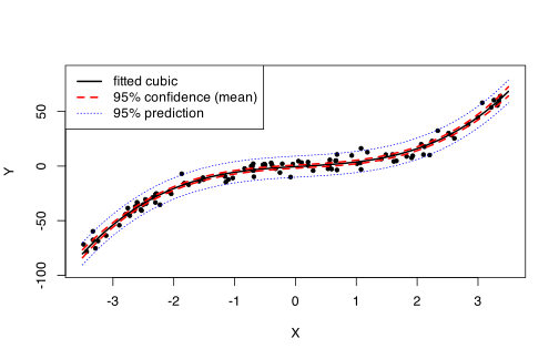
X fit lwr upr lwr upr
1 -3.5 -80.33 -84.00 -76.66 -90.59 -70.07
2 0.0 -0.55 -1.95 0.85 -10.24 9.13
3 3.5 68.38 64.18 72.59 57.92 78.85
The cubic follows the S shape of the cloud closely. The confidence band for the mean of \(Y\) (first lwr=/=upr pair) is narrow in the centre (\(\pm 1.4\) at \(X = 0\)) and widens at the edges of the data (\(\pm 4\) at \(X = \pm 3.5\)); the prediction band for a new observation (second pair) is much wider (\(\pm 9.7\) to \(\pm 10.5\)) because it adds the error variance \(\hat\sigma^2 = 4.83^2\), and it contains almost all the observed points, as expected of a 95% prediction interval.
Elementary analysis of variance
Exercises 15.1–15.7
Give the instruction to perform ANOVA with one factor (noted A).
summary(aov(Y ~ A)) (equivalently anova(lm(Y ~ A))), with A stored as a factor (Section 15.1). On the scarring-time data of Section 15.1:
X <- data.frame(Placebo = c(5,8,7,7,10,8), T2 = c(4,6,6,3,5,6),
T3 = c(6,4,4,5,4,3), T4 = c(7,4,6,6,3,5), T5 = c(9,3,5,7,7,6))
Y <- stack(X)$values ; A <- stack(X)$ind
summary(aov(Y ~ A))
Df Sum Sq Mean Sq F value Pr(>F)
A 4 36.47 9.117 3.896 0.0136 *
Residuals 25 58.50 2.340
---
Signif. codes: 0 '***' 0.001 '**' 0.01 '*' 0.05 '.' 0.1 ' ' 1
With \(p = 0.0136 < 0.05\) we reject \(H_0: \mu_1 = \dots = \mu_5\): at least two treatments have different mean scarring times.
Give the instruction to perform ANOVA with two factors (noted A and B) without interaction.
summary(aov(Y ~ A + B)) (or anova(lm(Y ~ A + B))): the + in the formula gives the additive model with main effects only. On the wheat data of Section 15.2.2 (A = region, B = fertilizer):
yield <- c(15,14,17,21,20,21,14,15,14,16,17,17,16,19,20,23,
24,25,15,14,14,12,11,12,18,17,17,20,21,21,17,19,17,12,13,13)
B <- gl(3, 12, 36, labels = paste("Fertilizer", 1:3))
A <- gl(4, 3, 36, labels = paste("Region", 1:4))
summary(aov(yield ~ A + B))
Df Sum Sq Mean Sq F value Pr(>F)
A 3 327.2 109.06 26.625 1.35e-08 ***
B 2 0.9 0.44 0.108 0.898
Residuals 30 122.9 4.10
---
Signif. codes: 0 '***' 0.001 '**' 0.01 '*' 0.05 '.' 0.1 ' ' 1
Under the additive model the region effect is highly significant (\(p = 1.35 \times 10^{-8}\)) while the fertilizer effect is not (\(p = 0.898\)); Exercise 15.3 shows this model omits a strong interaction.
Give the instruction to perform ANOVA with two factors (noted A and B) with interaction.
summary(aov(Y ~ A * B)) (or anova(lm(Y ~ A * B)), or car::Anova(lm(Y ~ A * B))), where A * B stands for A + B + A:B (Section 15.2.3). On the wheat data of Exercise 15.2 (same session):
summary(aov(yield ~ A * B))
Df Sum Sq Mean Sq F value Pr(>F)
A 3 327.2 109.06 112.181 2.95e-14 ***
B 2 0.9 0.44 0.457 0.638
A:B 6 99.6 16.59 17.067 1.36e-07 ***
Residuals 24 23.3 0.97
---
Signif. codes: 0 '***' 0.001 '**' 0.01 '*' 0.05 '.' 0.1 ' ' 1
The interaction is highly significant (\(p = 1.36 \times 10^{-7}\)): the effect of the fertilizer depends on the region, so the non-significant main effect of fertilizer must not be read as “no fertilizer effect”.
Which test would you use to check for homoscedasticity in an ANOVA model?
Bartlett’s test, bartlett.test(Y ~ A), or, when normality is doubtful, the more robust Levene test (Section 15.1.4); the levene.test() of the book and of the authors’ companion solution is defunct in current car, whose function is now leveneTest().
X <- data.frame(Placebo = c(5,8,7,7,10,8), T2 = c(4,6,6,3,5,6),
T3 = c(6,4,4,5,4,3), T4 = c(7,4,6,6,3,5), T5 = c(9,3,5,7,7,6))
Y <- stack(X)$values ; A <- stack(X)$ind
bartlett.test(Y ~ A)
car::leveneTest(Y ~ A)
Bartlett test of homogeneity of variances
data: Y by A
Bartlett's K-squared = 2.4197, df = 4, p-value = 0.6591
Levene's Test for Homogeneity of Variance (center = median)
Df F value Pr(>F)
group 4 0.5851 0.6763
25
Both \(p\)-values (0.66 and 0.68) are large, so equality of the five group variances is not rejected for the scarring-time data.
Which instruction performs pairwise tests after single-factor ANOVA?
pairwise.t.test(Y, A, p.adjust = "bonf"), which uses the pooled residual standard deviation and corrects for multiple testing through p.adjust (Section 15.1.5); TukeyHSD(aov(Y ~ A)) is the Tukey alternative. On the data of Exercise 15.4:
pairwise.t.test(Y, A, p.adjust = "bonf")
Pairwise comparisons using t tests with pooled SD
data: Y and A
Placebo T2 T3 T4
T2 0.090 - - -
T3 0.014 1.000 - -
T4 0.140 1.000 1.000 -
T5 1.000 1.000 0.483 1.000
P value adjustment method: bonferroni
After Bonferroni correction only the Placebo/T3 difference is significant at 5 % (adjusted \(p = 0.014\)).
Which function gives the estimates for a single-factor ANOVA model?
lm(), read through summary(lm(Y ~ A)) (or coef()); by default R imposes the constraint \(\alpha_1 = 0\), so the intercept estimates \(\mu_1\) and each other coefficient estimates \(\mu_i - \mu_1\) (Section 15.1.3). On the data of Exercise 15.4:
round(coef(summary(lm(Y ~ A))), 4)
Estimate Std. Error t value Pr(>|t|)
(Intercept) 7.5000 0.6245 12.0096 0.0000
AT2 -2.5000 0.8832 -2.8307 0.0090
AT3 -3.1667 0.8832 -3.5855 0.0014
AT4 -2.3333 0.8832 -2.6420 0.0140
AT5 -1.3333 0.8832 -1.5097 0.1437
The placebo mean is estimated at 7.5 days, and treatments T2, T3 and T4 shorten it significantly at the unadjusted 5 % level (by 2.5, 3.2 and 2.3 days), T5 does not (\(p = 0.14\)).
Which function is used to choose the constraint in ANOVA?
C(), applied to the factor inside the formula: C(A, base = 2) makes level 2 the reference (\(\alpha_2 = 0\)) and C(A, sum) imposes \(\sum_i \alpha_i = 0\) (Section 15.1.3); the contrasts argument of lm() does the same, e.g. contrasts = list(A = contr.sum).
round(coef(summary(lm(Y ~ C(A, sum)))), 4)
Estimate Std. Error t value Pr(>|t|)
(Intercept) 5.6333 0.2793 20.1706 0.0000
C(A, sum)1 1.8667 0.5586 3.3419 0.0026
C(A, sum)2 -0.6333 0.5586 -1.1338 0.2676
C(A, sum)3 -1.3000 0.5586 -2.3274 0.0283
C(A, sum)4 -0.4667 0.5586 -0.8355 0.4114
Under \(\sum_i \alpha_i = 0\) the intercept is the grand mean 5.63 days and each coefficient is a deviation of a treatment mean from it (the fifth is \(-\sum_{i \le 4} \hat\alpha_i = 0.53\)); the \(F\) test of Exercise 15.1 is unchanged.
Worksheet 15.W.A.1 — Study of one-way ANOVA - Study of noise levels
Worksheet 15.W.A.1 — Study of one-way ANOVA — Study of noise levels
In order to study the influence of the factor “level of surrounding noise” on the ability of a subject to solve a problem, the following experiment is designed: twenty-four school children are randomly allocated to four rooms. Street noises were previously recorded and are played in each room at a specific noise level. The children must solve a series of problems. The response variable is the final grade for the series of problems. The results are given in the following table (columns are the noise levels):
| 1 | 2 | 3 | 4 |
|---|---|---|---|
| 62 | 56 | 63 | 68 |
| 60 | 62 | 67 | 66 |
| 63 | 60 | 71 | 71 |
| 59 | 61 | 64 | 67 |
| 63 | 63 | 65 | 68 |
| 59 | 64 | 66 | 68 |
We wish to know whether there is an effect of the factor “level of surrounding noise” on a subject’s ability to solve a problem.
15.1- Input the data set in an adequate structure to perform ANOVA.
15.2- Write down the ANOVA model to answer the question.
15.3- Perform the analysis corresponding to your model.
15.4- Perform all pairwise comparisons of noise levels; remember to take into account the problem of multiplicity of tests.
15.1- A data frame in “long” format, one row per child, with the grade as a numeric column and the noise level as a factor; stack() does the reshaping, as in Section 15.1.2.
noise <- data.frame(N1 = c(62,60,63,59,63,59), N2 = c(56,62,60,61,63,64),
N3 = c(63,67,71,64,65,66), N4 = c(68,66,71,67,68,68))
grades <- stack(noise)
names(grades) <- c("grade", "level")
str(grades)
tapply(grades$grade, grades$level, mean)
'data.frame': 24 obs. of 2 variables:
$ grade: num 62 60 63 59 63 59 56 62 60 61 ...
$ level: Factor w/ 4 levels "N1","N2","N3",..: 1 1 1 1 1 1 2 2 2 2 ...
N1 N2 N3 N4
61 61 66 68
15.2- The one-way ANOVA model of Section 15.1.1, with \(I=4\) noise levels and \(n_i=6\) children per level:
\begin{equation*} Y_{ik} = \mu + \alpha_i + \varepsilon_{ik},\qquad i=1,\dots,4,\ k=1,\dots,6, \end{equation*}
where \(Y_{ik}\) is the grade of child \(k\) in room \(i\), the errors \(\varepsilon_{ik}\) are independent \(\mathcal{N}(0,\sigma^2)\), and R imposes the constraint \(\alpha_1=0\). The question is the test of \(H_0:\mu_1=\mu_2=\mu_3=\mu_4\) (i.e. \(\alpha_2=\alpha_3=\alpha_4=0\)) against \(H_1\): at least two means differ.
15.3- Fisher’s \(F\) test rejects \(H_0\): \(F=13.57\) on 3 and 20 df, \(p=4.7\times 10^{-5}\), so the noise level has a significant effect on the grade.
mod <- aov(grade ~ level, data = grades)
summary(mod)
bartlett.test(grade ~ level, data = grades)$p.value
shapiro.test(residuals(mod))$p.value
Df Sum Sq Mean Sq F value Pr(>F)
level 3 228 76.0 13.57 4.66e-05 ***
Residuals 20 112 5.6
---
Signif. codes: 0 ‘***’ 0.001 ‘**’ 0.01 ‘*’ 0.05 ‘.’ 0.1 ‘ ’ 1
[1] 0.5836931
[1] 0.862856
The assumptions hold: Bartlett’s test does not reject equal variances (\(p=0.58\)) and the Shapiro-Wilk test does not reject normality of the residuals (\(p=0.86\)).
15.4- pairwise.t.test() with Bonferroni’s correction (Section 15.1.5):
pairwise.t.test(grades$grade, grades$level, p.adjust = "bonf")
Pairwise comparisons using t tests with pooled SD
data: grades$grade and grades$level
N1 N2 N3
N2 1.00000 - -
N3 0.00934 0.00934 -
N4 0.00031 0.00031 0.95266
P value adjustment method: bonferroni
Since the design is balanced, Tukey’s method, which Section 15.1.5 calls the most accurate here, gives simultaneous intervals:
round(TukeyHSD(mod)$level, 4)
diff lwr upr p adj
N2-N1 0 -3.8241 3.8241 1.0000
N3-N1 5 1.1759 8.8241 0.0078
N4-N1 7 3.1759 10.8241 0.0003
N3-N2 5 1.1759 8.8241 0.0078
N4-N2 7 3.1759 10.8241 0.0003
N4-N3 2 -1.8241 5.8241 0.4766
Both corrections give the same conclusion at the 5 % level: levels 1 and 2 do not differ, levels 3 and 4 do not differ, but each of levels 3 and 4 gives significantly higher mean grades (by 5 and 7 points) than each of levels 1 and 2. The noise levels therefore form two groups, \(\{1,2\}\) and \(\{3,4\}\).
Worksheet 15.W.A.2 — Study of one-way ANOVA - Study of intima-media
Worksheet 15.W.A.2 — Study of one-way ANOVA — Study of intima-media
In the “Intima-media” study, we are interested in the relationship between intima-media thickness and alcohol consumption.
15.1- Download the intima-media data file.
15.2- Suggest a plot to visualize the differences in intima-media thickness depending on alcohol consumption.
15.3- Is there a difference of mean intima-media thickness depending on alcohol consumption?
15.4- Analyse the residuals to validate the assumptions of your statistical study.
15.1- read.table() with sep = " " (missing values are empty fields) and dec = ","; alcohol is recoded as a factor with the labels of Appendix B.3 (0 = non-drinker, 1 = occasional, 2 = regular drinker).
intima <- read.table("http://www.biostatisticien.eu/springeR/Intima_Media_Thickness.txt",
sep = " ", header = TRUE, dec = ",")
intima$alcohol <- factor(intima$alcohol, levels = 0:2,
labels = c("non-drinker", "occasional", "regular"))
table(intima$alcohol, useNA = "ifany")
round(tapply(intima$measure, intima$alcohol, mean), 3)
non-drinker occasional regular
23 71 16
non-drinker occasional regular
0.501 0.530 0.571
15.2- Parallel boxplots, plot(measure ~ alcohol) (Table 15.1), here with the group means added as red crosses.
plot(measure ~ alcohol, data = intima, xlab = "Alcohol consumption",
ylab = "Intima-media thickness (mm)", col = "grey90")
points(1:3, tapply(intima$measure, intima$alcohol, mean), pch = 4, col = "red", cex = 1.5)
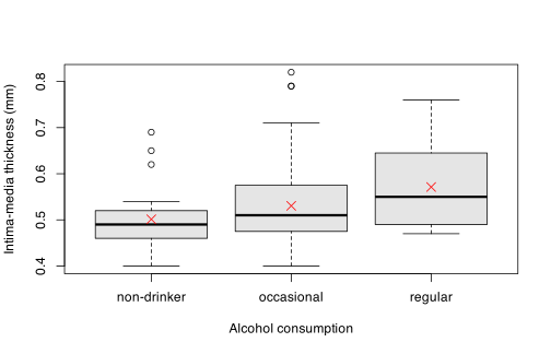
Thickness tends to increase with alcohol consumption, and the distributions are right-skewed (upper outliers).
15.3- Yes, at the 5 % level: in the model \(Y_{ik}=\mu+\alpha_i+\varepsilon_{ik}\) (\(i\) = alcohol class, \(\varepsilon_{ik}\) i.i.d. \(\mathcal{N}(0,\sigma^2)\)), Fisher’s test of \(H_0:\mu_1=\mu_2=\mu_3\) gives \(F=3.198\) on 2 and 107 df, \(p=0.045\).
mod <- aov(measure ~ alcohol, data = intima)
summary(mod)
Df Sum Sq Mean Sq F value Pr(>F)
alcohol 2 0.0462 0.023084 3.198 0.0448 *
Residuals 107 0.7723 0.007218
---
Signif. codes: 0 ‘***’ 0.001 ‘**’ 0.01 ‘*’ 0.05 ‘.’ 0.1 ‘ ’ 1
We reject \(H_0\) (just): mean intima-media thickness differs between alcohol classes, rising from 0.501 mm (non-drinkers) to 0.571 mm (regular drinkers).
15.4- Homoscedasticity holds but normality of the residuals does not: the four diagnostic plots of Section 15.1.4, Bartlett’s and Levene’s tests (the book’s levene.test() is now leveneTest() in car) and a Shapiro-Wilk test:
par(mfrow = c(2, 2))
plot(mod)
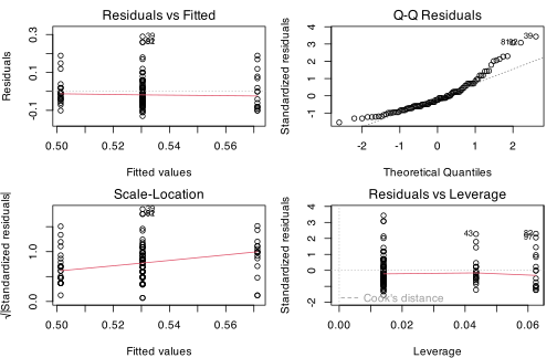
shapiro.test(residuals(mod))$p.value
bartlett.test(measure ~ alcohol, data = intima)$p.value
library(car)
leveneTest(measure ~ alcohol, data = intima)
kruskal.test(measure ~ alcohol, data = intima)$p.value
[1] 4.472462e-07
[1] 0.307024
Levene's Test for Homogeneity of Variance (center = median)
Df F value Pr(>F)
group 2 1.6941 0.1887
107
[1] 0.04435345
Homoscedasticity is acceptable (Bartlett \(p=0.31\), Levene \(p=0.19\); the “Residuals vs Fitted” spreads are comparable), but normality is not: the Q-Q plot bends upwards in the right tail (observations 39, 81, 92) and Shapiro-Wilk rejects with \(p=4.5\times10^{-7}\). With \(n=110\) the \(F\) test is fairly robust to this skewness, and the rank-based Kruskal-Wallis test, which does not assume normality, reaches the same conclusion (\(p=0.044\)), so the alcohol effect found in 15.3 stands, though only marginally.
Worksheet 15.W.A.3 — Study of one-way ANOVA - Study of physical activity
Worksheet 15.W.A.3 — Study of one-way ANOVA — Study of physical activity
In a study of risky behaviour amongst people aged 14 to 25, a scientist observed offences (theft, racketeering, brawls…) committed by youngsters and weekly physical activity. Risky behaviour was measured on a scale from 0 to 100. A subset of the data is available at the URL http://www.biostatisticien.eu/springeR/sports.RData:
> print(sports[sample(1:105,10),],row.names=FALSE)
score time
9 [2;3[
75 [0;1[
0 [3;4[
21 [2;3[
67 [4;5[
69 [1;2[
36 [2;3[
0 [3;4[
87 [0;1[
16 [2;3[
15.1- Describe the factors involved and write down the model (and the underlying assumptions).
15.2- Perform a test at the 5 % level to decide whether there is a significant effect between physical activity and risky behaviour.
We call “not athletic” youngsters who play sports for less than 2 hours per week, “somewhat athletic” those with weekly physical activity in the interval [2,4[ and “very athletic” those who play sports at least 4 hours per week. The scientist makes the following research assumptions:
research assumption 1: “not athletic” youngsters have more risky behaviour than “somewhat athletic” youngsters;
research assumption 2: risky behaviour is different between “very athletic” and “not athletic” youngsters.
15.3- Translate the research assumptions into contrasts.
15.4- Test these two assumptions at the 5 % level.
15.1- There is one factor, time (weekly hours of physical activity), with \(I=7\) modalities \([0;1[,\ [1;2[,\ \dots,\ [6;7[\), each observed on \(n_i=15\) youngsters; the response is the quantitative risky-behaviour score (0 to 100).
load(url("http://www.biostatisticien.eu/springeR/sports.RData"))
table(sports$time)
round(tapply(sports$score, sports$time, mean), 2)
[0;1[ [1;2[ [2;3[ [3;4[ [4;5[ [5;6[ [6;7[
15 15 15 15 15 15 15
[0;1[ [1;2[ [2;3[ [3;4[ [4;5[ [5;6[ [6;7[
76.40 57.67 28.33 30.33 52.00 68.73 79.07
The one-way ANOVA model (Section 15.1.1) is
\begin{equation*} Y_{ik} = \mu_i + \varepsilon_{ik} = \mu + \alpha_i + \varepsilon_{ik}, \qquad i=1,\dots,7,\ k=1,\dots,15, \end{equation*}
where \(Y_{ik}\) is the score of youngster \(k\) in activity class \(i\), \(\mu_i\) is the mean score of class \(i\), and the errors \(\varepsilon_{ik}\) are assumed independent, normally distributed, with mean 0 and a common variance \(\sigma^2\) (homoscedasticity); R uses the constraint \(\alpha_1=0\).
15.2- Physical activity has a highly significant effect on risky behaviour: Fisher’s test of \(H_0:\mu_1=\dots=\mu_7\) gives \(F=12.1\) on 6 and 98 df, \(p=3.9\times10^{-10}<0.05\).
mod <- aov(score ~ time, data = sports)
summary(mod)
bartlett.test(score ~ time, data = sports)$p.value
oneway.test(score ~ time, data = sports)$p.value
kruskal.test(score ~ time, data = sports)$p.value
Df Sum Sq Mean Sq F value Pr(>F)
time 6 38300 6383 12.1 3.86e-10 ***
Residuals 98 51679 527
---
Signif. codes: 0 ‘***’ 0.001 ‘**’ 0.01 ‘*’ 0.05 ‘.’ 0.1 ‘ ’ 1
[1] 1.291906e-09
[1] 1.290315e-14
[1] 3.000801e-08
Bartlett’s test rejects equal variances (\(p=1.3\times10^{-9}\); the group standard deviations range from 5.7 to 39.2), but the design is balanced, and Welch’s heteroscedastic test (oneway.test()) and the Kruskal-Wallis test both confirm the effect (\(p<10^{-7}\)).
15.3- With \(\mu_1,\dots,\mu_7\) the class means in the order above, “not athletic” is classes 1-2, “somewhat athletic” classes 3-4 and “very athletic” classes 5-7. The contrasts are
\begin{equation*} \begin{aligned} L_1 &= \tfrac12(\mu_1+\mu_2) - \tfrac12(\mu_3+\mu_4), &\lambda_1 &= (\tfrac12,\tfrac12,-\tfrac12,-\tfrac12,0,0,0)^T,\\ L_2 &= \tfrac13(\mu_5+\mu_6+\mu_7) - \tfrac12(\mu_1+\mu_2), &\lambda_2 &= (-\tfrac12,-\tfrac12,0,0,\tfrac13,\tfrac13,\tfrac13)^T, \end{aligned} \end{equation*}
(coefficients summing to zero), and the research assumptions become the alternatives: assumption 1 is \(H_0:L_1\le 0\) against \(H_1:L_1>0\) (one-sided), assumption 2 is \(H_0:L_2=0\) against \(H_1:L_2\ne 0\) (two-sided).
15.4- Assumption 1 is accepted, assumption 2 is not. fit.contrast() (Section 15.1.5; the book’s gregmisc has since been split and the function now lives in gmodels) gives two-sided \(p\)-values; the one-sided \(p\)-value for \(L_1\) is the upper tail of its \(t\) statistic.
library(gmodels)
cmat <- rbind(": not - somewhat" = c(1/2, 1/2, -1/2, -1/2, 0, 0, 0),
": very - not" = c(-1/2, -1/2, 0, 0, 1/3, 1/3, 1/3))
res <- fit.contrast(mod, "time", cmat)
res
pt(res[1, "t value"], df = df.residual(mod), lower.tail = FALSE)
Estimate Std. Error t value Pr(>|t|)
time: not - somewhat 37.7000000 5.929258 6.35829987 6.495787e-09
time: very - not -0.4333333 5.412647 -0.08005941 9.363533e-01
[1] 3.247894e-09
Research assumption 1: \(\hat L_1=37.7>0\) with one-sided \(p=3.2\times10^{-9}<0.05\), so “not athletic” youngsters have significantly more risky behaviour than “somewhat athletic” ones. Research assumption 2: \(\hat L_2=-0.43\), \(p=0.94>0.05\), so no difference in risky behaviour is detected between “very athletic” and “not athletic” youngsters; the relationship is U-shaped, with the lowest scores for 2 to 4 hours of sport per week.
Worksheet 15.W.B.1 — Study of two-way ANOVA - Study of batteries
Worksheet 15.W.B.1 — Study of two-way ANOVA — Study of batteries
In an experiment on battery lifetime, the aim is to find battery life as a function of type of battery. It is known that battery lifetime depends on temperature, so a plane with two factors (temperature and type of battery) is created. The following table gives battery lifetime depending on these two factors.
| 15 \(^\circ\)C | 70 \(^\circ\)C | 125 \(^\circ\)C | |
|---|---|---|---|
| Type I | 130 155 | 34 40 | 20 70 |
| 74 180 | 80 75 | 82 58 | |
| Type II | 150 188 | 136 122 | 25 70 |
| 159 126 | 106 115 | 58 45 | |
| Type III | 138 110 | 174 120 | 96 104 |
| 168 160 | 150 139 | 82 60 |
15.1- Which factors are involved in this experiment? What are their modalities? What is the response variable?
15.2- Propose and define an ANOVA model for this data set.
15.3- Propose a graphical representation to visualize any interaction there may be in the model.
15.4- Estimate the parameters of the model.
15.5- Draw an ANOVA table for your model.
15.6- Perform the relevant tests to finalize this analysis.
15.1- Two crossed factors: battery type (modalities I, II, III) and temperature (modalities 15 \(^\circ\)C, 70 \(^\circ\)C, 125 \(^\circ\)C); the response is battery lifetime. Each of the \(3\times 3\) cells holds 4 observations, so the design is balanced (\(n=36\)). The data are entered in the style of Section 15.2.2:
life <- c(130,155,74,180, 34,40,80,75, 20,70,82,58,
150,188,159,126, 136,122,106,115, 25,70,58,45,
138,110,168,160, 174,120,150,139, 96,104,82,60)
type <- gl(3, 12, labels = c("I", "II", "III"))
temp <- gl(3, 4, 36, labels = c("15C", "70C", "125C"))
battery <- data.frame(life, type, temp)
with(battery, tapply(life, list(type, temp), mean))
15C 70C 125C
I 134.75 57.25 57.5
II 155.75 119.75 49.5
III 144.00 145.75 85.5
15.2- The two-way ANOVA model with interaction of Section 15.2.1:
\begin{equation*} Y_{ijk} = \mu_{\bullet\bullet} + \alpha_i^A + \alpha_j^B + \beta_{ij} + \varepsilon_{ijk}, \qquad i,j = 1,2,3,\quad k = 1,\dots,4, \end{equation*}
where \(Y_{ijk}\) is the lifetime of the \(k\)-th battery of type \(i\) at temperature \(j\), \(\alpha_i^A\) is the differential effect of type \(i\), \(\alpha_j^B\) that of temperature \(j\), \(\beta_{ij}\) the interaction effect, and the errors \(\varepsilon_{ijk}\) are independent \(N(0,\sigma^2)\) (so \(Y_{ijk}\sim N(\mu_{ij},\sigma^2)\), a common variance in all nine cells).
15.3- An interaction plot (interaction.plot(), Section 15.2.2), drawn both ways round:
par(mfrow = c(1, 2))
with(battery, interaction.plot(temp, type, life, ylab = "mean lifetime"))
with(battery, interaction.plot(type, temp, life, ylab = "mean lifetime"))
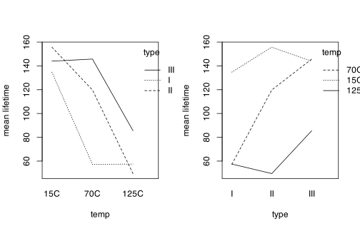
The profiles are far from parallel: type I collapses already at 70 \(^\circ\)C, whereas type III keeps its lifetime up to 70 \(^\circ\)C, which suggests an interaction.
15.4- Under R’s constraints \(\alpha_1^A=\alpha_1^B=0\), \(\beta_{1j}=\beta_{i1}=0\) (Section 15.2.3) the estimates are the lm()=/=aov() coefficients; model.tables() gives the grand and marginal means, from which the differential effects of Section 15.2.1 follow.
mod <- aov(life ~ type * temp, data = battery)
round(coef(mod), 2)
lapply(model.tables(mod, type = "means")$tables[1:3], round, 2)
sigma(lm(life ~ type * temp, data = battery))^2
(Intercept) typeII typeIII temp70C
134.75 21.00 9.25 -77.50
temp125C typeII:temp70C typeIII:temp70C typeII:temp125C
-77.25 41.50 79.25 -29.00
typeIII:temp125C
18.75
$`Grand mean`
[1] 105.53
$type
type
I II III
83.17 108.33 125.08
$temp
temp
15C 70C 125C
144.83 107.58 64.17
[1] 675.213
The intercept \(134.75\) is the mean lifetime of type I at 15 \(^\circ\)C, and every other cell mean is the intercept plus its main-effect and interaction terms (e.g. type III at 70 \(^\circ\)C: \(134.75+9.25-77.5+79.25=145.75\)). With the sum-to-zero constraints of Section 15.2.1, \(\hat\mu_{\bullet\bullet}=105.53\), \(\hat\alpha^A=(-22.36,\,2.81,\,19.56)\) for types I, II, III, \(\hat\alpha^B=(39.31,\,2.06,\,-41.36)\) for 15, 70, 125 \(^\circ\)C, and \(\hat\sigma^2=675.2\) on 27 df.
15.5- The ANOVA table is given by summary(aov()) (Section 15.2.3; the design is balanced, so the sequential decomposition is unique):
summary(mod)
Df Sum Sq Mean Sq F value Pr(>F)
type 2 10684 5342 7.911 0.00198 **
temp 2 39119 19559 28.968 1.91e-07 ***
type:temp 4 9614 2403 3.560 0.01861 *
Residuals 27 18231 675
---
Signif. codes: 0 ‘***’ 0.001 ‘**’ 0.01 ‘*’ 0.05 ‘.’ 0.1 ‘ ’ 1
15.6- The interaction test (\(H_0:\beta_{ij}=0\) for all \(i,j\)) gives \(F=3.56\), \(p=0.019<0.05\): the interaction between type and temperature is significant, so the model with interaction is kept and, as Section 15.2.3 advises, the main effects are not interpreted from the table; instead the type effect is tested at each temperature, dividing the one-way mean square by the residual mean square of the full model (27 df). The model assumptions are checked first (Bartlett test over the nine cells, Shapiro-Wilk on the residuals).
bartlett.test(life ~ interaction(type, temp), data = battery)$p.value
shapiro.test(residuals(mod))$p.value
CMres <- deviance(mod) / df.residual(mod)
sapply(levels(battery$temp), function(t) {
s <- summary(aov(life ~ type, data = battery, subset = temp == t))[[1]]
F <- s[1, "Mean Sq"] / CMres
c(F = F, p.value = pf(F, 2, df.residual(mod), lower.tail = FALSE))
}) |> signif(3)
library(emmeans)
pairs(emmeans(mod, ~ type | temp, at = list(temp = "70C")))
[1] 0.7321499
[1] 0.6117267
15C 70C 125C
F 0.656 1.23e+01 2.12
p.value 0.527 1.63e-04 0.14
temp = 70C:
contrast estimate SE df t.ratio p.value
I - II -62.5 18.4 27 -3.402 0.0058
I - III -88.5 18.4 27 -4.817 0.0001
II - III -26.0 18.4 27 -1.415 0.3475
P value adjustment: tukey method for comparing a family of 3 estimates
Homoscedasticity (\(p=0.73\)) and normality (\(p=0.61\)) are not rejected, so the tests are valid. Battery type makes no significant difference at 15 \(^\circ\)C (\(p=0.53\)) or at 125 \(^\circ\)C (\(p=0.14\)), but it does at 70 \(^\circ\)C (\(p=1.6\times 10^{-4}\)), where types II and III both last significantly longer than type I (Tukey-adjusted comparisons with the pooled residual variance) and do not differ from each other. Every type loses lifetime at 125 \(^\circ\)C (interaction plot), and type III, never significantly worse than the others and with the highest mean at 70 \(^\circ\)C and 125 \(^\circ\)C, is the most robust choice.
Worksheet 15.W.B.2 — Study of two-way ANOVA - Milk yield
Worksheet 15.W.B.2 — Study of two-way ANOVA — Milk yield
We are interested in the influence of type and quantity of food on milk yield. We have observed these forty values:
| Straw | Hay | Grass | Silage | |
|---|---|---|---|---|
| Low dose | 8 11 11 10 7 | 12 13 14 11 10 | 10 12 12 13 14 | 17 13 17 14 13 |
| High dose | 8 9 8 10 9 | 10 7 10 12 11 | 11 9 11 11 12 | 13 12 11 15 14 |
15.1- Propose and define an ANOVA model to study the influence of type and quantity of food on milk yield.
15.2- Propose a graphical representation to visualize any interaction there may be in the model.
15.3- Estimate the parameters of the model.
15.4- Draw an ANOVA table for your model.
15.5- Perform the relevant tests to finalize this analysis.
15.1- A two-way ANOVA with interaction (Section 15.2.1), with factor A = dose (low, high; \(I=2\)) and factor B = type of food (straw, hay, grass, silage; \(J=4\)), five cows per cell:
\begin{equation*} Y_{ijk} = \mu_{\bullet\bullet} + \alpha_i^A + \alpha_j^B + \beta_{ij} + \varepsilon_{ijk}, \qquad i=1,2,\quad j=1,\dots,4,\quad k=1,\dots,5, \end{equation*}
where \(Y_{ijk}\) is the milk yield, \(\alpha_i^A\) and \(\alpha_j^B\) the differential effects of dose \(i\) and food \(j\), \(\beta_{ij}\) their interaction, and \(\varepsilon_{ijk}\) independent \(N(0,\sigma^2)\) errors.
yield <- c(8,11,11,10,7, 12,13,14,11,10, 10,12,12,13,14, 17,13,17,14,13,
8,9,8,10,9, 10,7,10,12,11, 11,9,11,11,12, 13,12,11,15,14)
dose <- gl(2, 20, labels = c("Low", "High"))
food <- gl(4, 5, 40, labels = c("Straw", "Hay", "Grass", "Silage"))
milk <- data.frame(yield, dose, food)
with(milk, tapply(yield, list(dose, food), mean))
Straw Hay Grass Silage
Low 9.4 12 12.2 14.8
High 8.8 10 10.8 13.0
15.2- An interaction plot of the cell means:
with(milk, interaction.plot(food, dose, yield, ylab = "mean milk yield"))
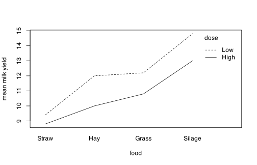
The two dose profiles are almost parallel (the high dose sits 0.6 to 2 units below the low dose for every food), so little or no interaction is expected.
15.3- With R’s constraints (first level of each factor as reference, Section 15.2.3):
mod <- aov(yield ~ dose * food, data = milk)
round(coef(mod), 2)
lapply(model.tables(mod, type = "means")$tables[1:3], round, 2)
deviance(mod) / df.residual(mod)
(Intercept) doseHigh foodHay foodGrass
9.4 -0.6 2.6 2.8
foodSilage doseHigh:foodHay doseHigh:foodGrass doseHigh:foodSilage
5.4 -1.4 -0.8 -1.2
$`Grand mean`
[1] 11.38
$dose
dose
Low High
12.10 10.65
$food
food
Straw Hay Grass Silage
9.1 11.0 11.5 13.9
[1] 2.5125
The intercept 9.4 is the mean yield with a low dose of straw; e.g. high-dose silage has mean \(9.4-0.6+5.4-1.2=13.0\). With the sum-to-zero constraints, \(\hat\mu_{\bullet\bullet}=11.38\), \(\hat\alpha^A=(0.725,\,-0.725)\) for low/high dose, \(\hat\alpha^B=(-2.275,\,-0.375,\,0.125,\,2.525)\) for straw, hay, grass, silage, and \(\hat\sigma^2=2.51\) on 32 df.
15.4- The ANOVA table (balanced design):
summary(mod)
Df Sum Sq Mean Sq F value Pr(>F)
dose 1 21.03 21.03 8.368 0.00682 **
food 3 117.07 39.02 15.532 2.07e-06 ***
dose:food 3 2.87 0.96 0.381 0.76705
Residuals 32 80.40 2.51
---
Signif. codes: 0 ‘***’ 0.001 ‘**’ 0.01 ‘*’ 0.05 ‘.’ 0.1 ‘ ’ 1
15.5- The interaction is not significant (\(F=0.38\), \(p=0.77>0.05\)), so, following Section 15.2.3, the additive model \(Y_{ijk}=\mu_{\bullet\bullet}+\alpha_i^A+\alpha_j^B+\varepsilon_{ijk}\) is fitted and its main effects tested; the assumptions and the pairwise food comparisons are checked on it.
mod2 <- aov(yield ~ dose + food, data = milk)
summary(mod2)
round(coef(mod2), 2)
bartlett.test(yield ~ interaction(dose, food), data = milk)$p.value
shapiro.test(residuals(mod2))$p.value
TukeyHSD(mod2, "food")$food |> round(4)
Df Sum Sq Mean Sq F value Pr(>F)
dose 1 21.03 21.03 8.837 0.00531 **
food 3 117.07 39.02 16.402 7.98e-07 ***
Residuals 35 83.27 2.38
---
Signif. codes: 0 ‘***’ 0.001 ‘**’ 0.01 ‘*’ 0.05 ‘.’ 0.1 ‘ ’ 1
(Intercept) doseHigh foodHay foodGrass foodSilage
9.83 -1.45 1.90 2.40 4.80
[1] 0.8013939
[1] 0.3546157
diff lwr upr p adj
Hay-Straw 1.9 0.0396 3.7604 0.0438
Grass-Straw 2.4 0.5396 4.2604 0.0071
Silage-Straw 4.8 2.9396 6.6604 0.0000
Grass-Hay 0.5 -1.3604 2.3604 0.8865
Silage-Hay 2.9 1.0396 4.7604 0.0010
Silage-Grass 2.4 0.5396 4.2604 0.0071
Variances are homogeneous (\(p=0.80\)) and the residuals normal (\(p=0.35\)). Both factors act on milk yield: the dose effect is significant (\(p=0.005\), the high dose giving on average 1.45 units less than the low dose) and so is the type of food (\(p=8\times 10^{-7}\)). Silage gives the highest yield (significantly above all other foods), straw the lowest, and hay and grass do not differ (\(p=0.89\)).
Worksheet 15.W.B.3 — Study of two-way ANOVA - Intima-media study
Worksheet 15.W.B.3 — Study of two-way ANOVA — Intima-media study
In practical A, we looked at a possible relationship between intima-media thickness and alcohol consumption in the “Intima-media” study. We now wonder whether intima-media thickness is linked to alcohol consumption and tobacco consumption.
15.1- Download the intima-media data set.
15.2- Propose and define an ANOVA model to study the influence of tobacco consumption and alcohol consumption on intima-media thickness.
15.3- Propose a graphical representation to visualize any interaction there may be in the model.
15.4- Is there a difference in intima-media thickness depending on alcohol consumption? Depending on tobacco consumption?
15.1- read.table() on the book’s text file (Section 4.1.1: space separator, comma decimal mark), with the two codes turned into labelled factors (the book’s description of the data set codes tobacco 0/1/2 = non-smoker/former smoker/smoker, alcohol 0/1/2 = non-drinker/occasional/regular drinker):
imt <- read.table("http://www.biostatisticien.eu/springeR/Intima_Media_Thickness.txt",
header = TRUE, sep = " ", dec = ",")
imt$tobacco <- factor(imt$tobacco, levels = 0:2,
labels = c("non-smoker", "former smoker", "smoker"))
imt$alcohol <- factor(imt$alcohol, levels = 0:2,
labels = c("non-drinker", "occasional", "regular"))
with(imt, table(tobacco, alcohol))
alcohol
tobacco non-drinker occasional regular
non-smoker 18 45 9
former smoker 3 14 1
smoker 2 12 6
The 110 subjects are spread very unevenly over the nine cells (from 1 to 45 per cell): the design is unbalanced.
15.2- The two-way ANOVA model with interaction of Section 15.2.1, with A = tobacco (\(I=3\)) and B = alcohol (\(J=3\)):
\begin{equation*} Y_{ijk} = \mu_{\bullet\bullet} + \alpha_i^A + \alpha_j^B + \beta_{ij} + \varepsilon_{ijk}, \qquad i,j=1,2,3,\quad k=1,\dots,n_{ij}, \end{equation*}
where \(Y_{ijk}\) is the intima-media thickness (mm) of the \(k\)-th subject with tobacco status \(i\) and alcohol consumption \(j\), \(\alpha_i^A\), \(\alpha_j^B\) and \(\beta_{ij}\) are the tobacco, alcohol and interaction effects, and the \(\varepsilon_{ijk}\) are independent \(N(0,\sigma^2)\). Because \(n_{ij}\) varies, the tests use type III sums of squares (Section 15.2.2).
15.3- The interaction plot of the cell means:
with(imt, interaction.plot(alcohol, tobacco, measure,
ylab = "mean intima-media thickness (mm)"))
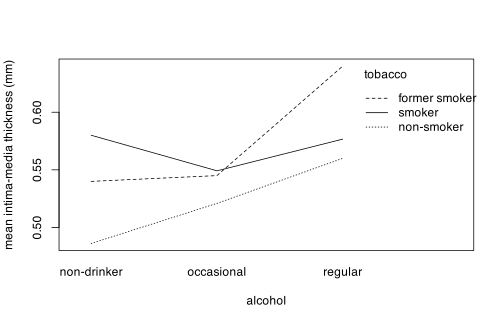
The profiles cross (smokers do not follow the upward trend with alcohol seen in non-smokers), but the most extreme point, former smokers who drink regularly, rests on a single subject, so the apparent interaction may be noise.
15.4- Neither: once both factors are in the model, neither alcohol nor tobacco has a significant effect at the 5 % level. The interaction is tested first (type III, contrasts as in Section 15.2.3), then, since it is not significant, the additive model \(Y_{ijk}=\mu_{\bullet\bullet}+\alpha_i^A+\alpha_j^B+\varepsilon_{ijk}\) is fitted and its main effects tested (type II, each adjusted for the other).
library(car)
mod <- lm(measure ~ tobacco * alcohol, data = imt,
contrasts = list(tobacco = contr.sum, alcohol = contr.sum))
options(show.signif.stars = FALSE)
Anova(mod, type = "III")
mod2 <- lm(measure ~ tobacco + alcohol, data = imt)
Anova(mod2, type = "II")
round(coef(mod2), 3)
shapiro.test(residuals(mod2))$p.value
Anova(lm(log(measure) ~ tobacco + alcohol, data = imt))[1:2, 4]
Anova Table (Type III tests)
Response: measure
Sum Sq Df F value Pr(>F)
(Intercept) 10.6579 1 1466.6124 <2e-16
tobacco 0.0314 2 2.1608 0.1205
alcohol 0.0187 2 1.2892 0.2800
tobacco:alcohol 0.0118 4 0.4061 0.8039
Residuals 0.7340 101
Anova Table (Type II tests)
Response: measure
Sum Sq Df F value Pr(>F)
tobacco 0.02655 2 1.8692 0.15934
alcohol 0.03531 2 2.4854 0.08818
Residuals 0.74577 105
(Intercept) tobaccoformer smoker tobaccosmoker
0.494 0.033 0.033
alcoholoccasional alcoholregular
0.024 0.063
[1] 2.254354e-07
[1] 0.09781140 0.08086831
There is no interaction (\(p=0.80\)). In the additive model the alcohol effect (\(p=0.088\)) and the tobacco effect (\(p=0.16\)) are both non-significant, even though the estimated thickness rises with alcohol (+0.024 mm for occasional, +0.063 mm for regular drinkers) and is about 0.033 mm higher for smokers and former smokers than for non-smokers. So the alcohol effect found in the one-way analysis of practical A (15.W.A.2, \(p=0.045\)) does not survive adjustment for tobacco, to which it is partly confounded. The residuals are not normal (Shapiro-Wilk \(p=2.3\times 10^{-7}\), right skew), but with \(n=110\) the \(F\) tests are robust, and a log-transformed response gives the same verdict (\(p=0.098\) for tobacco, \(p=0.081\) for alcohol).
Backlinks (2)
1. The R Software: Fundamentals of Programming and Statistical Analysis /words/library/books/the-r-software/
Pierre Lafaye de Micheaux, Rémy Drouilhet and Benoît Liquet, The R Software: Fundamentals of Programming and Statistical Analysis, Springer Statistics and Computing 40, 2013 (translated from the French Le logiciel R). Part I introduces R and the book’s data sets; Part II covers the language (data structures, import/export, manipulation and functions, documentation, plots, programming, sessions); Part III applies it to matrices and optimisation, descriptive statistics, random variables and simulation, confidence intervals and tests, linear regression and ANOVA. Chapters 3 to 15 each end with exercises and a practical worksheet.
2. Books /words/library/books/
Here are the books that I have taken the time to create metadata and/or notes for.
Comments