Optimiser Paradigms in Machine Learning
deep learning pipeline
Recall that a Neural Network follows the following construction:
- Pass data (forward) through model to get predicted values
- Calculate loss with predicted values against labels
- Perform backpropagation w.r.t each weight / bias to get the direction in which to move that weight such that it moves closer to the global minima
- Update parameters with gradients using an optimiser.
momentum
ball’s pace slows down this makes total fkn sense! if the gradient signs are the same, increasing your confidence in that direction and move further. you want to take less steps over all
optimisers
sgd
you want to take less steps over all
vanilla
\[W_{t+1} = W_t - \alpha\nabla W_t \]
with momentum
\[V_{t+1} = \beta V_t + (1-\beta)\nabla W_t\\ W_{t+1} = W_t - \alpha V_{t+1}\\ \beta = 0.9\]
clearly if you unroll the \(V_{t+1}\) term, you are equivalently unrolling the exponential weighted average: \[\begin{align*} V_{t+1} &= \beta V_t + (1-\beta)\nabla W_t\\ V_{t+2} &= \beta [\beta V_t + (1-\beta)\nabla W_t] + (1-\beta)\nabla W_t\\ &= \beta^2 V_t + \beta(1-\beta)\nabla W_t + (1-\beta)\nabla W_t \end{align*}\]
which represents all the subsequently older gradients with more decayed contributions to the current gradient; nonetheless they are contributive.
nag (Nesterov Accelerated Gradient)
is also an option. it adds a corrective term to sgd momentum:
from \[V_{t+1} = \beta V_t + (1-\beta)\nabla W_t\] to \[V_{t+1} = \beta V_t + \alpha \nabla(W_t - \beta V_t)\]
algorithm
from the pytorch site:
\[\begin{aligned} &\rule{110mm}{0.4pt} \\ &\textbf{input} : \gamma \text{ (lr)}, \theta_0 \text{ (params)}, f(\theta) \text{ (objective)}, \lambda \text{ (weight decay)}, \\ &\hspace{13mm} \mu \text{ (momentum)}, \tau \text{ (dampening)}, \textit{ nesterov, maximize} \[-1.ex] &\rule{110mm}{0.4pt} \\ &\textbf{for} \quad t=1 \quad \textbf{to} \quad \ldots \quad \textbf{do} \\ &\hspace{5mm} g_t \leftarrow \nabla_{\theta} f_t (\theta_{t-1}) \\ &\hspace{5mm} \textbf{if} \quad \lambda \neq 0 \\ &\hspace{10mm} g_t \leftarrow g_t + \lambda \theta_{t-1} \\ &\hspace{5mm} \textbf{if} \quad \mu \neq 0 \\ &\hspace{10mm} \textbf{if} \quad t > 1 \\ &\hspace{15mm} \mathbf{b}_t \leftarrow \mu \mathbf{b}_{t-1} + (1 - \tau) g_t \\ &\hspace{10mm} \textbf{else} \\ &\hspace{15mm} \mathbf{b}_t \leftarrow g_t \\ &\hspace{5mm} \textbf{if} \quad \textit{nesterov} \\ &\hspace{10mm} g_t \leftarrow g_t + \mu \mathbf{b}_t \\ &\hspace{5mm} \textbf{if} \quad \textit{maximize} \\ &\hspace{10mm} \theta_t \leftarrow \theta_{t-1} + \gamma g_t \\ &\hspace{5mm} \textbf{else} \\ &\hspace{10mm} \theta_t \leftarrow \theta_{t-1} - \gamma g_t \\ &\rule{110mm}{0.4pt} \\ &\textbf{return} \quad \theta_t \end{aligned}\]
limitations
if the gradients become really small, then you’ll move towards the minimum really slowly.
this can happen with sparse data.
rms prop (Root Mean-Squared Propagation)
the key feature is that this optimiser can adjust the learning rate for each parameter. it steals the idea from ada grad (Adaptive Gradients).
\[V_{t+1} = \beta V_t + (1-\beta)\nabla W_t^2\\ W_{t+1} = W_t - \alpha \frac{\nabla W_t}{\sqrt{V_{t+1}+\epsilon}}\\ \beta = 0.9\qquad\text{(compare apples with apples)}\]
ada grad
ada grad does not weight down older gradients. \[V_{t+1} = V_t + \nabla W_t^2\\ W_{t+1} = W_t - \alpha \frac{\nabla W_t}{\sqrt{V_{t+1}+\epsilon}}\quad\text{(this is the same)}\]
ada delta
limits the number of past gradients that are included in the calculation of how to modulate the learning rate.
adam (Adaptive Moment Estimation)
combination of momentum and adaptive gradients
the first moment is referred to as the mean. if the magnitude of the mean is higher that indicates the gradients are pointing in the same direction.
variance, or squared-error is the second moment. this is what rms prop uses to modulate the learning rates individually for each parameter (based on its gradients).{{< mnote “we are only calculating the uncentered variance (not substracting from the mean” >}}. high variance -> smaller steps, variance low -> bigger steps.
\[\begin{align} M_t &= \beta_1 M_{t-1} + (1-\beta_1)\nabla W_t \\ V_t &= \beta_2 V_{t-1} + (1-\beta_2)\nabla W_t^2 \\ \hat{M}_t &= \cfrac{M_t}{1-\beta_1^t}\\ \hat{V}_t &= \cfrac{V_t}{1-\beta_2^t}\\ W_{t+1} &= W_t -\alpha \cfrac{\hat{M}_t}{\sqrt{\hat{V}_t}+\epsilon}\\ \beta_1 &= 0.9\\ \beta_2 &= 0.99\\ \epsilon &= 10^{-8}\\ \end{align}\]
might delete:
\[\begin{align} M_t &= \beta_1 M_{t-1} + (1-\beta_1)\nabla W_t \\ V_t &= \beta_2 V_{t-1} + (1-\beta_2)\nabla W_t^2 \\ \left.\begin{aligned}[t] \hat{M}_t &= \cfrac{M_t}{1-\beta_1^t}\\ \hat{V}_t &= \cfrac{V_t}{1-\beta_2^t} \end{aligned}\right\} \text{ bias correction} \\ W_{t+1} &= W_t -\alpha \cfrac{\hat{M}_t}{\sqrt{\hat{V}_t}+\epsilon}\\ \beta_1 &= 0.9\\ \beta_2 &= 0.99\\ \epsilon &= 10^{-8}\\ \end{align}\]
experiments
resnet 18
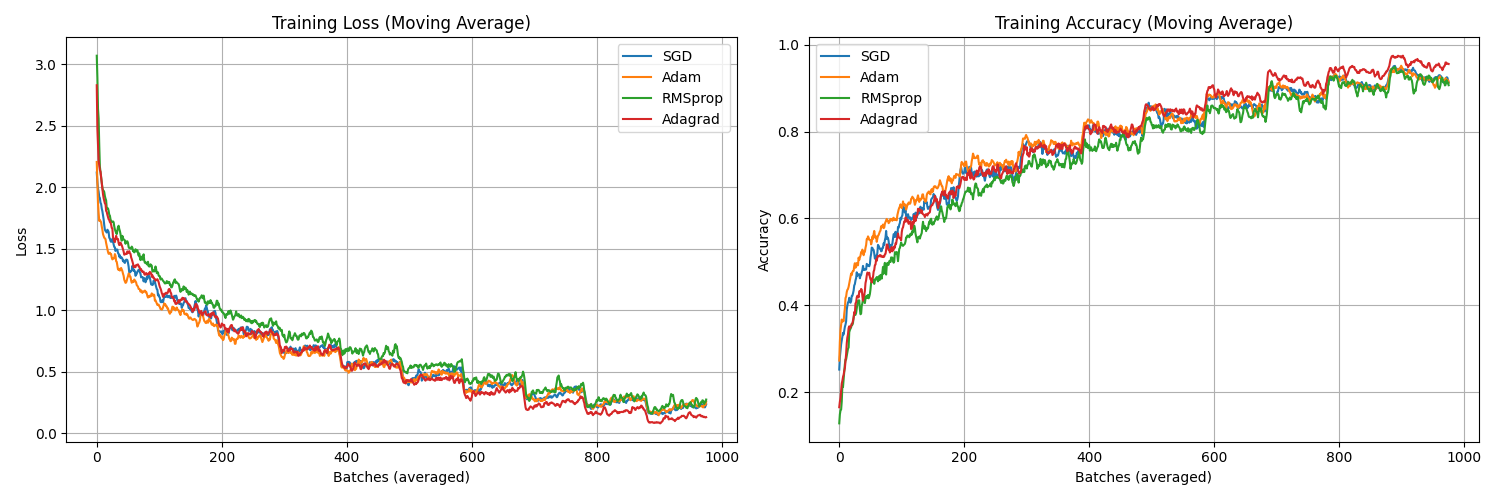
I retrained the final fully-connected layer across 10 epochs
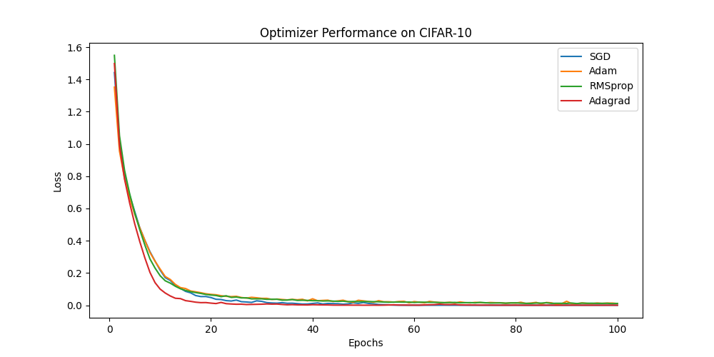
to see a little more detail claude helped me split the epochs into smaller batches
code
import torch
import torch.nn as nn
import torch.optim as optim
import torchvision
import torchvision.transforms as transforms
import matplotlib.pyplot as plt
from torchvision.models import resnet18
import numpy as np

# Device Configuration
device = torch.device("cuda" if torch.cuda.is_available() else "cpu")

# Data Transformations
transform = transforms.Compose([
    transforms.ToTensor(),
    transforms.Normalize((0.5,), (0.5,))
])

# Load CIFAR-10
trainset = torchvision.datasets.CIFAR10(root='./data', train=True, download=True, transform=transform)
trainloader = torch.utils.data.DataLoader(trainset, batch_size=256, shuffle=True, num_workers=2)  # Doubled batch size

testset = torchvision.datasets.CIFAR10(root='./data', train=False, download=True, transform=transform)
testloader = torch.utils.data.DataLoader(testset, batch_size=256, shuffle=False, num_workers=2)  # Doubled batch size

# Define Model
model = resnet18(weights=None)  # No pretrained weights
model.fc = nn.Linear(512, 10)  # Adjust final layer for 10 classes
model = model.to(device)

# Loss Function
criterion = nn.CrossEntropyLoss()

# Define Optimizers
optimizers = {
    "SGD": optim.SGD(model.parameters(), lr=0.01, momentum=0.9),
    "Adam": optim.Adam(model.parameters(), lr=0.001),
    "RMSprop": optim.RMSprop(model.parameters(), lr=0.001),
    "Adagrad": optim.Adagrad(model.parameters(), lr=0.01)
}

# Training Parameters
epochs = 10
# Store loss and accuracy for plotting, with batch-level granularity
history = {name: {'loss': [], 'accuracy': []} for name in optimizers}

def compute_accuracy(outputs, labels):
    _, predicted = torch.max(outputs.data, 1)
    total = labels.size(0)
    correct = (predicted == labels).sum().item()
    return correct / total

# Training Loop
for name, optimizer in optimizers.items():
    print(f"\nTraining with {name} optimizer...")
    model.apply(lambda m: m.reset_parameters() if hasattr(m, "reset_parameters") else None)  # Reset weights

    batch_count = 0
    for epoch in range(epochs):
        model.train()
        running_loss = 0.0
        running_accuracy = 0.0
        samples_counted = 0

        for images, labels in trainloader:
            images, labels = images.to(device), labels.to(device)

            optimizer.zero_grad()
            outputs = model(images)
            loss = criterion(outputs, labels)
            loss.backward()
            optimizer.step()

            # Compute accuracy
            accuracy = compute_accuracy(outputs, labels)

            # Accumulate metrics
            running_loss += loss.item()
            running_accuracy += accuracy
            samples_counted += 1

            # Store averaged metrics every 2 batches
            if samples_counted == 2:
                history[name]['loss'].append(running_loss / 2)
                history[name]['accuracy'].append(running_accuracy / 2)
                running_loss = 0.0
                running_accuracy = 0.0
                samples_counted = 0

                batch_count += 1
                if batch_count % 25 == 0:  # Print less frequently since we're averaging
                    print(f"Epoch [{epoch+1}/{epochs}], Batch [{batch_count}], "
                          f"Loss: {history[name]['loss'][-1]:.4f}, "
                          f"Accuracy: {history[name]['accuracy'][-1]:.4f}")

# Create subplots for loss and accuracy
fig, (ax1, ax2) = plt.subplots(1, 2, figsize=(15, 5))

# Plot Loss with moving average
window = 5  # Window size for moving average
for name, metrics in history.items():
    losses = metrics['loss']
    # Calculate moving average
    smoothed_losses = np.convolve(losses, np.ones(window)/window, mode='valid')
    ax1.plot(smoothed_losses, label=name)
ax1.set_xlabel("Batches (averaged)")
ax1.set_ylabel("Loss")
ax1.set_title("Training Loss (Moving Average)")
ax1.legend()
ax1.grid(True)

# Plot Accuracy with moving average
for name, metrics in history.items():
    accuracies = metrics['accuracy']
    # Calculate moving average
    smoothed_accuracies = np.convolve(accuracies, np.ones(window)/window, mode='valid')
    ax2.plot(smoothed_accuracies, label=name)
ax2.set_xlabel("Batches (averaged)")
ax2.set_ylabel("Accuracy")
ax2.set_title("Training Accuracy (Moving Average)")
ax2.legend()
ax2.grid(True)

plt.tight_layout()
plt.savefig("training_metrics.png")
plt.close()
environment (earth)
better optimiser, means less ruining earth.
reinforcement learning
rmsprop might be better than adam because as the agent explores new areas of the environment the distribution of training data tends to shift. what used to be the best action towards the beginning of the game, may not continue to be so later on in the game.
thus, samples rl are not i.i.d. and momentum may be a detriment to performance.
memory
for each parameter, we store 2 extra values, as such adam is the least memory efficient optimiser; tripling memory usage.
just taking notes for the moment. a video by Sourish Kundu
references
Backlinks (3)
1. Wiki /wiki/
Knowledge is a paradox. The more one understand, the more one realises the vastness of his ignorance.
2. Backpropagation /wiki/ml/theory/backprop/
“Back-propagation is often misunderstood as meaning the whole learning algorithm for multi layer neural networks” — Deep Learning (2015), Bengio
Backpropagation{{< mnote “lovingly abbreviated to backprop” >}} is the process of computing the derivatives of the loss function recursively through a computation graph with respect to each of its weights. Another algorithm, usually some flavour of gradient descent is used to perform learning with this gradient.
It is worth drawing a few lines in the sand from the getgo:
3. Machine Learning /wiki/ml/
Type 1 error